Planar Differential Systems Qualitative Theory of
316
-
Upload
khangminh22 -
Category
Documents
-
view
0 -
download
0
Transcript of Planar Differential Systems Qualitative Theory of

123
Freddy Dumortier, Jaume Llibre, Joan C. Artés
Planar Differential SystemsQualitative Theory of
With 123 Figures and 10 Tables
ISBN-10 Springer Berlin Heidelberg New YorkISBN-13 Springer Berlin Heidelberg New York
This work is subject to copyright. All rights are reserved, whether the whole or part of the materialis concerned, specifically the rights of translation, reprinting, reuse of illustrations, recitation,broadcasting, reproduction on microfilm or in any other way, and storage in data banks. Dupli-cation of this publication or parts thereof is permitted only under the provisions of the GermanCopyright Law of September 9, 1965, in its current version, and permission for use must always beobtained from Springer. Violations are liable for prosecution under the German Copyright Law.
Springer is a part of Springer Science+Business Media
The use of general descriptive names, registered names, trademarks, etc. in this publication doesnot imply, even in the absence of a specific statement, that such names are exempt from the relevantprotective laws and regulations and therefore free for general use.
Cover design: Erich Kirchner, HeidelbergA
E
Printed on acid-free paper
Freddy DumortierHasselt UniversityCampus DiepenbeekAgoralaan-Gebouw D3590 Diepenbeek, Belgiume-mail: [email protected]
Universitat Aut noma deBarcelona
Barcelona, Spaine-mail: [email protected]
Universitat Aut noma de
Barcelona, Spaine-mail: [email protected]
Library of Congress Control Number: 2006924563
Mathematics Subject Classification (2000): 34Cxx (34C05, 34C07, 34C08, 34C14, 34C20,
34C25, 34C37, 34C41), 37Cxx (37C10, 37C15, 37C20, 37C25, 37C27, 37C29)
springer.com
ò
ò
é
08193 Cerdanyola
08193 Cerdanyola
3-540-32893-9
© Springer-Verlag Berlin Heidelberg 2006
3-540-32902-1
Jaume Llibre
Joan C. Art s
Barcelona
using a Springer LT X macro packageTypesetting by the authors and SPi
Dept. Matem tiques
Dept. Matem tiques
á
á
SPIN: 11371328 41/3100/SPi 5 4 3 2 1 0
Preface
Our aim is to study ordinary differential equations or simply differential sys-tems in two real variables
x = P (x, y),
y = Q(x, y),(0.1)
where P and Q are Cr functions defined on an open subset U of R2, withr = 1, 2, . . . ,∞, ω. As usual Cω stands for analyticity. We put special emphasisonto polynomial differential systems, i.e., on systems (0.1) where P and Q arepolynomials.
Instead of talking about the differential system (0.1), we frequently talkabout its associated vector field
X = P (x, y)∂
∂x+ Q(x, y)
∂
∂y(0.2)
on U ⊂ R2. This will enable a coordinate-free approach, which is typical inthe theory of dynamical systems. Another way expressing the vector field is bywriting it as X = (P,Q). In fact, we do not distinguish between the differentialsystem (0.1) and its vector field (0.2).
Almost all the notions and results that we present for two-dimensionaldifferential systems can be generalized to higher dimensions and manifolds;but our goal is not to present them in general, we want to develop all thesenotions and results in dimension 2. We would like this book to be a niceintroduction to the qualitative theory of differential equations in the plane,providing simultaneously the major part of concepts and ideas for developinga similar theory on more general surfaces and in higher dimensions. Exceptin very limited cases we do not deal with bifurcations, but focus on the studyof individual systems.
Our goal is certainly not to look for an analytic expression of the globalsolutions of (0.1). Not only would it be an impossible task for most differentialsystems, but even in the few cases where a precise analytic expression can befound it is not always clear what it really represents. Numerical analysis of a
VI Preface
differential system (0.1) together with graphical representation are essentialingredients in the description of the phase portrait of a system (0.1) on U ; thatis, the description of U as union of all the orbits of the system. Of course,we do not limit our study to mere numerical integration. In fact in tryingto do this one often encounters serious problems; calculations can take anenormous amount of time or even lead to erroneous results. Based howeveron a priori knowledge of some essential results on differential systems (0.1),these problems can often be avoided.
Qualitative techniques are very appropriate to get such an overall under-standing of a differential system (0.1). A clear picture is achieved by drawinga phase portrait in which the relevant qualitative features are represented;it often suffices to draw the “extended separatrix skeleton.” Of course, forpractical reasons, the representation must not be too far from reality andhas to respect some numerical accuracy. These are, in a nutshell, the mainingredients in our approach.
The basic results on differential systems and their qualitative theory areintroduced in Chap. 1. There we present the fundamental theorems of exis-tence, uniqueness, and continuity of the solutions of a differential system withrespect the initial conditions, the notions of α- and ω-limit sets of an orbit,the Poincare–Bendixson theorem characterizing these limit sets and the use ofLyapunov functions in studying stability and asymptotic stability. We analyzethe local behavior of the orbits near singular points and periodic orbits. Weintroduce the notions of separatrix, separatrix skeleton, extended (and com-pleted) separatrix skeleton, and canonical region that are basic ingredients forthe characterization of a phase portrait.
The study of the singular points is the main objective of Chaps. 2, 3, 4,and 6, and partially of Chap. 5. In Chap. 2 we mainly study the elementarysingular points, i.e., the hyperbolic and semi-hyperbolic singular points. Wealso provide the normal forms for such singularities providing complete proofsbased on an appropriate two-dimensional approach and with full attention tothe best regularity properties of the invariant curves. In Chap. 3, we providethe basic tool for studying all singularities of a differential system in the plane,this tool being based on convenient changes of variables called blow-ups. Weuse this technique for classifying the nilpotent singularities.
A serious problem consists in distinguishing between a focus and a center.This problem is unsolved in general, but in the case where the singular pointis a linear center there are algorithms for solving it. In Chap. 4 we present thebest of these algorithms currently available.
Polynomial differential systems are defined in the whole plane R2. Thesesystems can be extended to infinity, compactifying R2 by adding a circle,and extending analytically the flow to this boundary. This is done by the so-called “Poincare compactification,” and also by the more general “Poincare–Lyapunov compactification.” In both cases we get an extended analytic differ-ential system on the closed disk. In this way, we can study the behavior of theorbits near infinity. The singular points that are on the circle at infinity are
Preface VII
called the infinite singular points of the initial polynomial differential system.Suitably gluing together two copies of the extended system, we get an analyticdifferential system on the two-dimensional sphere.
In Chap. 6 we associate an integer to every isolated singular point of a two-dimensional differential system, called its index. We prove the Poincare–Hopftheorem for vector fields on the sphere that have finitely many singularities:the sum of the indices is 2. We also present the Poincare formula for computingthe index of an isolated singular point.
After singular points the main subjects of two-dimensional differential sys-tems are limit cycles, i.e., periodic orbits that are isolated in the set of allperiodic orbits of a differential system. In Chap. 7 we present the more basicresults on limit cycles. In particular, we show that any topological configura-tion of limit cycles is realizable by a convenient polynomial differential system.We define the multiplicity of a limit cycle, and we study the bifurcations oflimit cycles for rotated families of vector fields. We discuss structural stability,presenting a number of results and some open problems. We do not providecomplete proofs but explain some steps in the exercises.
For a two-dimensional vector field the existence of a first integral com-pletely determines its phase portrait. Since for such vector fields the notion ofintegrability is based on the existence of a first integral the following naturalquestion arises: Given a vector field on R2, how can one determine if thisvector field has a first integral? The easiest planar vector fields having a firstintegral are the Hamiltonian ones. The integrable planar vector fields that arenot Hamiltonian are, in general, very difficult to detect. In Chap. 8 we studythe existence of first integrals for planar polynomial vector fields through theDarbouxian theory of integrability. This kind of integrability provides a linkbetween the integrability of polynomial vector fields and the number of in-variant algebraic curves that they have.
In Chap. 9 we present a computer program based on the tools introducedin the previous chapters. The program is an extension of previous work dueto J. C. Artes and J. Llibre and strongly relies on ideas of F. Dumortier andthe thesis of C. Herssens. Recently, P. De Maesschalck had made substan-tial adaptations. The program is called “Polynomial Planar Phase Portraits,”abbreviated as P4 [9]. This program is designed to draw the phase portraitof any polynomial differential system on the compactified plane obtained byPoincare or Poincare–Lyapunov compactification; local phase portraits, e.g.,near singularities in the finite plane or at infinity, can also be obtained. Ofcourse, there are always some computational limitations that are described inChaps. 9 and 10. This last chapter is dedicated to illustrating the use of theprogram P4.
Almost all chapters end with a series of appropriate exercises and somebibliographic comments.
The program P4 is freeware and the reader may download it at will fromhttp://mat.uab.es/∼artes/p4/p4.htm at no cost. The program does not in-clude either MAPLE or REDUCE, which are registered programs and must
VIII Preface
be acquired separately from P4. The authors have checked it to be bug free,but nevertheless the reader may eventually run into a problem that P4 (orthe symbolic program) cannot deal with, not even by modifying the workingparameters.
To end this preface we would like to thank Douglas Shafer from the Univer-sity of North Carolina at Charlotte for improving the presentation, especiallythe use of the English language, in a previous version of the book.
Contents
1 Basic Results on the Qualitative Theory of DifferentialEquations . . . . . . . . . . . . . . . . . . . . . . . . . . . . . . . . . . . . . . . . . . . . . . . . . 11.1 Vector Fields and Flows . . . . . . . . . . . . . . . . . . . . . . . . . . . . . . . . . . 11.2 Phase Portrait of a Vector Field . . . . . . . . . . . . . . . . . . . . . . . . . . . 41.3 Topological Equivalence and Conjugacy . . . . . . . . . . . . . . . . . . . . 81.4 α- and ω-limits Sets of an Orbit . . . . . . . . . . . . . . . . . . . . . . . . . . . 111.5 Local Structure of Singular Points . . . . . . . . . . . . . . . . . . . . . . . . . 141.6 Local Structure Near Periodic Orbits . . . . . . . . . . . . . . . . . . . . . . 201.7 The Poincare–Bendixson Theorem . . . . . . . . . . . . . . . . . . . . . . . . 241.8 Lyapunov Functions . . . . . . . . . . . . . . . . . . . . . . . . . . . . . . . . . . . . . 301.9 Essential Ingredients of Phase Portraits . . . . . . . . . . . . . . . . . . . . 331.10 Exercises . . . . . . . . . . . . . . . . . . . . . . . . . . . . . . . . . . . . . . . . . . . . . . . 351.11 Bibliographical Comments . . . . . . . . . . . . . . . . . . . . . . . . . . . . . . . . 41
2 Normal Forms and Elementary Singularities . . . . . . . . . . . . . . . 432.1 Formal Normal Form Theorem . . . . . . . . . . . . . . . . . . . . . . . . . . . 432.2 Attracting (Repelling) Hyperbolic Singularities . . . . . . . . . . . . . 462.3 Hyperbolic Saddles . . . . . . . . . . . . . . . . . . . . . . . . . . . . . . . . . . . . . . 49
2.3.1 Analytic Results . . . . . . . . . . . . . . . . . . . . . . . . . . . . . . . . . . 492.3.2 Smooth Results . . . . . . . . . . . . . . . . . . . . . . . . . . . . . . . . . . . 52
2.4 Topological Study of Hyperbolic Saddles . . . . . . . . . . . . . . . . . . . 552.5 Semi-Hyperbolic Singularities . . . . . . . . . . . . . . . . . . . . . . . . . . . . 59
2.5.1 Analytic and Smooth Results . . . . . . . . . . . . . . . . . . . . . . . 592.5.2 Topological Results . . . . . . . . . . . . . . . . . . . . . . . . . . . . . . . . 682.5.3 More About Center Manifolds . . . . . . . . . . . . . . . . . . . . . . 69
2.6 Summary on Elementary Singularities . . . . . . . . . . . . . . . . . . . . . . 712.7 Removal of Flat Terms . . . . . . . . . . . . . . . . . . . . . . . . . . . . . . . . . . . 76
2.7.1 Generalities . . . . . . . . . . . . . . . . . . . . . . . . . . . . . . . . . . . . . . . 762.7.2 Hyperbolic Case . . . . . . . . . . . . . . . . . . . . . . . . . . . . . . . . . . . 792.7.3 Semi-Hyperbolic Case . . . . . . . . . . . . . . . . . . . . . . . . . . . . . . 81
2.8 Exercises . . . . . . . . . . . . . . . . . . . . . . . . . . . . . . . . . . . . . . . . . . . . . . . 842.9 Bibliographical Comments . . . . . . . . . . . . . . . . . . . . . . . . . . . . . . . . 88
X Contents
3 Desingularization of Nonelementary Singularities . . . . . . . . . 913.1 Homogeneous Blow-Up . . . . . . . . . . . . . . . . . . . . . . . . . . . . . . . . . . 913.2 Desingularization and the �Lojasiewicz Property . . . . . . . . . . . . . 983.3 Quasihomogeneous blow-up . . . . . . . . . . . . . . . . . . . . . . . . . . . . . . . 1023.4 Nilpotent Singularities . . . . . . . . . . . . . . . . . . . . . . . . . . . . . . . . . . . 107
3.4.1 Hamiltonian Like Case (m < 2n + 1) . . . . . . . . . . . . . . . . . 1093.4.2 Singular Like Case (m > 2n + 1) . . . . . . . . . . . . . . . . . . . . 1103.4.3 Mixed Case (m = 2n + 1) . . . . . . . . . . . . . . . . . . . . . . . . . . 112
3.5 Summary on Nilpotent Singularities . . . . . . . . . . . . . . . . . . . . . . . 1163.6 Exercises . . . . . . . . . . . . . . . . . . . . . . . . . . . . . . . . . . . . . . . . . . . . . . . 1183.7 Bibliographical Comments . . . . . . . . . . . . . . . . . . . . . . . . . . . . . . . . 120
4 Centers and Lyapunov Constants . . . . . . . . . . . . . . . . . . . . . . . . . . 1214.1 Introduction . . . . . . . . . . . . . . . . . . . . . . . . . . . . . . . . . . . . . . . . . . . . 1214.2 Normal Form for Linear Centers . . . . . . . . . . . . . . . . . . . . . . . . . . . 1224.3 The Main Result . . . . . . . . . . . . . . . . . . . . . . . . . . . . . . . . . . . . . . . . 1244.4 Basic Results . . . . . . . . . . . . . . . . . . . . . . . . . . . . . . . . . . . . . . . . . . . 1274.5 The Algorithm . . . . . . . . . . . . . . . . . . . . . . . . . . . . . . . . . . . . . . . . . . 133
4.5.1 A Theoretical Description . . . . . . . . . . . . . . . . . . . . . . . . . . 1334.5.2 Practical Implementation . . . . . . . . . . . . . . . . . . . . . . . . . . . 141
4.6 Applications . . . . . . . . . . . . . . . . . . . . . . . . . . . . . . . . . . . . . . . . . . . . 1424.6.1 Known Examples . . . . . . . . . . . . . . . . . . . . . . . . . . . . . . . . . . 1434.6.2 Kukles-Homogeneous Family . . . . . . . . . . . . . . . . . . . . . . . . 144
4.7 Bibliographical Comments . . . . . . . . . . . . . . . . . . . . . . . . . . . . . . . . 147
5 Poincare and Poincare–Lyapunov Compactification . . . . . . . 1495.1 Local Charts . . . . . . . . . . . . . . . . . . . . . . . . . . . . . . . . . . . . . . . . . . . . 1495.2 Infinite Singular Points . . . . . . . . . . . . . . . . . . . . . . . . . . . . . . . . . . . 1545.3 Poincare–Lyapunov Compactification . . . . . . . . . . . . . . . . . . . . . . 1565.4 Bendixson Compactification . . . . . . . . . . . . . . . . . . . . . . . . . . . . . . 1565.5 Global Flow of a Planar Polynomial Vector Field . . . . . . . . . . . . 1575.6 Exercises . . . . . . . . . . . . . . . . . . . . . . . . . . . . . . . . . . . . . . . . . . . . . . . 1615.7 Bibliographical Comments . . . . . . . . . . . . . . . . . . . . . . . . . . . . . . . . 162
6 Indices of Planar Singular Points . . . . . . . . . . . . . . . . . . . . . . . . . 1656.1 Index of a Closed Path Around a Point . . . . . . . . . . . . . . . . . . . . . 1656.2 Deformations of Paths . . . . . . . . . . . . . . . . . . . . . . . . . . . . . . . . . . . 1686.3 Continuous Maps of the Closed Disk . . . . . . . . . . . . . . . . . . . . . . . 1706.4 Vector Fields Along the Unit Circle . . . . . . . . . . . . . . . . . . . . . . . . 1706.5 Index of Singularities of a Vector Field . . . . . . . . . . . . . . . . . . . . . 1726.6 Vector Fields on the Sphere S2 . . . . . . . . . . . . . . . . . . . . . . . . . . . . 1766.7 Poincare Index Formula . . . . . . . . . . . . . . . . . . . . . . . . . . . . . . . . . . 1796.8 Relation Between Index and Multiplicity . . . . . . . . . . . . . . . . . . . 1816.9 Exercises . . . . . . . . . . . . . . . . . . . . . . . . . . . . . . . . . . . . . . . . . . . . . . . 1836.10 Bibliographical Comments . . . . . . . . . . . . . . . . . . . . . . . . . . . . . . . . 183

Contents XI
7 Limit Cycles and Structural Stability . . . . . . . . . . . . . . . . . . . . . 1857.1 Basic Results . . . . . . . . . . . . . . . . . . . . . . . . . . . . . . . . . . . . . . . . . . . 1857.2 Configuration of Limit Cycles and Algebraic Limit Cycles . . . . 1927.3 Multiplicity and Stability of Limit Cycles . . . . . . . . . . . . . . . . . . . 1957.4 Rotated Vector Fields . . . . . . . . . . . . . . . . . . . . . . . . . . . . . . . . . . . . 1967.5 Structural Stability . . . . . . . . . . . . . . . . . . . . . . . . . . . . . . . . . . . . . . 2017.6 Exercises . . . . . . . . . . . . . . . . . . . . . . . . . . . . . . . . . . . . . . . . . . . . . . . 2047.7 Bibliographical Comments . . . . . . . . . . . . . . . . . . . . . . . . . . . . . . . . 210
8 Integrability and Algebraic Solutions in PolynomialVector Fields . . . . . . . . . . . . . . . . . . . . . . . . . . . . . . . . . . . . . . . . . . . . . 2138.1 Introduction . . . . . . . . . . . . . . . . . . . . . . . . . . . . . . . . . . . . . . . . . . . . 2138.2 First Integrals and Invariants . . . . . . . . . . . . . . . . . . . . . . . . . . . . . 2148.3 Integrating Factors . . . . . . . . . . . . . . . . . . . . . . . . . . . . . . . . . . . . . . 2148.4 Invariant Algebraic Curves . . . . . . . . . . . . . . . . . . . . . . . . . . . . . . . 2158.5 Exponential Factors . . . . . . . . . . . . . . . . . . . . . . . . . . . . . . . . . . . . . 2178.6 The Method of Darboux . . . . . . . . . . . . . . . . . . . . . . . . . . . . . . . . . . 2198.7 Some Applications of the Darboux Theory . . . . . . . . . . . . . . . . . . 2238.8 Prelle–Singer and Singer Results . . . . . . . . . . . . . . . . . . . . . . . . . . 2288.9 Exercises . . . . . . . . . . . . . . . . . . . . . . . . . . . . . . . . . . . . . . . . . . . . . . . 2298.10 Bibliographical Comments . . . . . . . . . . . . . . . . . . . . . . . . . . . . . . . . 230
9 Polynomial Planar Phase Portraits . . . . . . . . . . . . . . . . . . . . . . . . 2339.1 The Program P4 . . . . . . . . . . . . . . . . . . . . . . . . . . . . . . . . . . . . . . . . 2339.2 Technical Overview . . . . . . . . . . . . . . . . . . . . . . . . . . . . . . . . . . . . . . 2419.3 Attributes of Interface Windows . . . . . . . . . . . . . . . . . . . . . . . . . . . 242
9.3.1 The Planar Polynomial Phase Portraits Window . . . . . . 2429.3.2 The Phase Portrait Window . . . . . . . . . . . . . . . . . . . . . . . . 2469.3.3 The Plot Orbits Window . . . . . . . . . . . . . . . . . . . . . . . . . . . 2519.3.4 The Parameters of Integration Window . . . . . . . . . . . . . . 2529.3.5 The Greatest Common Factor Window . . . . . . . . . . . . . . . 2539.3.6 The Plot Separatrices Window . . . . . . . . . . . . . . . . . . . . . . 2549.3.7 The Limit Cycles Window . . . . . . . . . . . . . . . . . . . . . . . . . . 2559.3.8 The Print Window . . . . . . . . . . . . . . . . . . . . . . . . . . . . . . . . 256
10 Examples for Running P4 . . . . . . . . . . . . . . . . . . . . . . . . . . . . . . . . . 25910.1 Some Basic Examples . . . . . . . . . . . . . . . . . . . . . . . . . . . . . . . . . . . . 25910.2 Modifying Parameters . . . . . . . . . . . . . . . . . . . . . . . . . . . . . . . . . . . . 26410.3 Systems with Weak Foci or Limit Cycles . . . . . . . . . . . . . . . . . . . 27310.4 Exercises . . . . . . . . . . . . . . . . . . . . . . . . . . . . . . . . . . . . . . . . . . . . . . . 279
Bibliography . . . . . . . . . . . . . . . . . . . . . . . . . . . . . . . . . . . . . . . . . . . . . . . . . . . 285
Index . . . . . . . . . . . . . . . . . . . . . . . . . . . . . . . . . . . . . . . . . . . . . . . . . . . . . . . . . . 295
List of Figures
1.1 An integral curve . . . . . . . . . . . . . . . . . . . . . . . . . . . . . . . . . . . . . . . . . 21.2 Phase portrait of Example 1.7 . . . . . . . . . . . . . . . . . . . . . . . . . . . . . 71.3 Phase portraits of Example 1.8 . . . . . . . . . . . . . . . . . . . . . . . . . . . . . 71.4 The Flow Box Theorem . . . . . . . . . . . . . . . . . . . . . . . . . . . . . . . . . . . 91.5 The arc {ϕ(t, p) : t ∈ [0, t0]} . . . . . . . . . . . . . . . . . . . . . . . . . . . . . . . 111.6 A limit cycle and some orbits spiralling to it . . . . . . . . . . . . . . . . . 121.7 A subsequence converging to a point of a limit cycle . . . . . . . . . . 141.8 Sectors near a singular point . . . . . . . . . . . . . . . . . . . . . . . . . . . . . . . 181.9 Curves surrounding a point p . . . . . . . . . . . . . . . . . . . . . . . . . . . . . . 191.10 Local behavior near a periodic orbit . . . . . . . . . . . . . . . . . . . . . . . . 211.11 Different classes of limit cycles and their Poincare maps . . . . . . . 221.12 Scheme of the section . . . . . . . . . . . . . . . . . . . . . . . . . . . . . . . . . . . . . 251.13 Scheme of flow across the section . . . . . . . . . . . . . . . . . . . . . . . . . . . 261.14 Definition of Jordan’s curve . . . . . . . . . . . . . . . . . . . . . . . . . . . . . . . . 271.15 Impossible configurations . . . . . . . . . . . . . . . . . . . . . . . . . . . . . . . . . . 271.16 Possible configuration . . . . . . . . . . . . . . . . . . . . . . . . . . . . . . . . . . . . . 271.17 Periodic orbit as ω-limit . . . . . . . . . . . . . . . . . . . . . . . . . . . . . . . . . . . 281.18 Possible ω-limit sets . . . . . . . . . . . . . . . . . . . . . . . . . . . . . . . . . . . . . . 291.19 A singular point as ω-limit . . . . . . . . . . . . . . . . . . . . . . . . . . . . . . . . 291.20 A saddle-node loop . . . . . . . . . . . . . . . . . . . . . . . . . . . . . . . . . . . . . . . 311.21 Figure for Exercise 1.5 . . . . . . . . . . . . . . . . . . . . . . . . . . . . . . . . . . . . 361.22 Hint for Exercise 1.14 . . . . . . . . . . . . . . . . . . . . . . . . . . . . . . . . . . . . . 39
2.1 Transverse section around an attracting singular point . . . . . . . . 472.2 The flow on the boundary of V0 . . . . . . . . . . . . . . . . . . . . . . . . . . . . 532.3 A hyperbolic saddle . . . . . . . . . . . . . . . . . . . . . . . . . . . . . . . . . . . . . . . . 552.4 The transition close to a saddle . . . . . . . . . . . . . . . . . . . . . . . . . . . . 562.5 Modified transition close to a saddle . . . . . . . . . . . . . . . . . . . . . . . . 572.6 Comparing transitions close to two saddles . . . . . . . . . . . . . . . . . . 582.7 Flows of system (2.28) . . . . . . . . . . . . . . . . . . . . . . . . . . . . . . . . . . . . 612.8 Flow near a center manifold when λ > 0 . . . . . . . . . . . . . . . . . . . . . 64
XIV List of Figures
2.9 Flow near a center manifold when λ < 0 . . . . . . . . . . . . . . . . . . . . . 652.10 Saddle–nodes . . . . . . . . . . . . . . . . . . . . . . . . . . . . . . . . . . . . . . . . . . . . 682.11 Transition close to a semi-hyperbolic point . . . . . . . . . . . . . . . . . . 692.12 Phase portraits of non–degenerate singular points . . . . . . . . . . . . 722.13 Phase portraits of semi-hyperbolic singular points . . . . . . . . . . . . 74
3.1 Blow-up of Example 3.1 . . . . . . . . . . . . . . . . . . . . . . . . . . . . . . . . . . . 943.2 Local phase portrait of Example 3.1 . . . . . . . . . . . . . . . . . . . . . . . . 953.3 Successive blowing up . . . . . . . . . . . . . . . . . . . . . . . . . . . . . . . . . . . . . 973.4 Blowing up Example 3.2 . . . . . . . . . . . . . . . . . . . . . . . . . . . . . . . . . . 983.5 Local phase portrait of Example 3.2 . . . . . . . . . . . . . . . . . . . . . . . . 983.6 Some singularities of X on ∂An . . . . . . . . . . . . . . . . . . . . . . . . . . . . 993.7 Samples of desingularizations of monodromic orbits . . . . . . . . . . . 1003.8 Blowing up a hyperbolic sector . . . . . . . . . . . . . . . . . . . . . . . . . . . . . 1013.9 Blowing up an elliptic sector . . . . . . . . . . . . . . . . . . . . . . . . . . . . . . . 1013.10 Blowing up of part of adjacent elliptic sectors . . . . . . . . . . . . . . . . 1023.11 Quasihomogeneous blow-up of the cusp singularity . . . . . . . . . . . . 1043.12 Calculating the Newton polygon. . . . . . . . . . . . . . . . . . . . . . . . . . . . 1053.13 Desingularization of Hamiltonian like case when m is odd . . . . . 1103.14 Desingularization of Hamiltonian like case when m even . . . . . . . 1113.15 Blow-ups of the singular like case . . . . . . . . . . . . . . . . . . . . . . . . . . . 1113.16 Phase portraits of the singular like case . . . . . . . . . . . . . . . . . . . . . 1123.17 Blow-ups of the mixed case . . . . . . . . . . . . . . . . . . . . . . . . . . . . . . . . 1133.18 Phase portraits of the mixed case . . . . . . . . . . . . . . . . . . . . . . . . . . . 1133.19 Phase portrait of (3.23) . . . . . . . . . . . . . . . . . . . . . . . . . . . . . . . . . . . 1153.20 Phase portrait of (3.24) . . . . . . . . . . . . . . . . . . . . . . . . . . . . . . . . . . . 1163.21 Phase portraits of nilpotent singular points . . . . . . . . . . . . . . . . . . 117
5.1 The local charts (Uk, φk) for k = 1, 2, 3 of the Poincare sphere . . 1515.2 A hyperbolic or semi-hyperbolic saddle on the equator of S2 . . . 1555.3 Saddle-nodes of type SN1 and SN2 of p(X) in the equator of S2 1555.4 The phase portrait in the Poincare disk of system (5.11) . . . . . . . 1585.5 The phase portrait in the Poincare disk of system (5.12) . . . . . . . 1595.6 The phase portrait in the Poincare disk of system (5.13) . . . . . . . 1605.7 Compactification of system (5.15) . . . . . . . . . . . . . . . . . . . . . . . . . . 1615.8 Compactification of system (5.16) . . . . . . . . . . . . . . . . . . . . . . . . . . 1615.9 Phase portraits of Exercise 5.2 . . . . . . . . . . . . . . . . . . . . . . . . . . . . . 1625.10 Phase portraits of quadratic homogenous systems . . . . . . . . . . . . 163
6.1 Same image, different paths . . . . . . . . . . . . . . . . . . . . . . . . . . . . . . . . 1666.2 Definition of ϕ(t) . . . . . . . . . . . . . . . . . . . . . . . . . . . . . . . . . . . . . . . . . 1666.3 Some examples of indices . . . . . . . . . . . . . . . . . . . . . . . . . . . . . . . . . . 1676.4 Examples of homotopic closed paths . . . . . . . . . . . . . . . . . . . . . . . . 1696.5 Closed path associated to a vector field . . . . . . . . . . . . . . . . . . . . . 1716.6 Point of index −1 . . . . . . . . . . . . . . . . . . . . . . . . . . . . . . . . . . . . . . . . 174

List of Figures XV
6.7 Point of index 2 . . . . . . . . . . . . . . . . . . . . . . . . . . . . . . . . . . . . . . . . . . 1756.8 Piecing of D
2 . . . . . . . . . . . . . . . . . . . . . . . . . . . . . . . . . . . . . . . . . . . . 1756.9 Stereographic projection for example 6.29 . . . . . . . . . . . . . . . . . . . 1776.10 Phase portraits for example 6.29 . . . . . . . . . . . . . . . . . . . . . . . . . . . 1776.11 The vector fields X ′ and X ′′ on D
2 . . . . . . . . . . . . . . . . . . . . . . . . . 1786.12 Index given by sectors . . . . . . . . . . . . . . . . . . . . . . . . . . . . . . . . . . . . 181
7.1 A limit cycle with a node inside . . . . . . . . . . . . . . . . . . . . . . . . . . . . 2047.2 A limit cycle surrounding a saddle, two antisaddles, and two
limit cycles in different nests . . . . . . . . . . . . . . . . . . . . . . . . . . . . . . . 204
9.1 Representation of the Poincare–Lyapunov disk of degree (α, β) . 2419.2 The Planar Polynomial Phase Portraits window . . . . . . . . . . . . . . 2429.3 The Main settings window . . . . . . . . . . . . . . . . . . . . . . . . . . . . . . . . . 2439.4 The Output window . . . . . . . . . . . . . . . . . . . . . . . . . . . . . . . . . . . . . . 2459.5 The Poincare Disc window . . . . . . . . . . . . . . . . . . . . . . . . . . . . . . . . 2479.6 The Legend window . . . . . . . . . . . . . . . . . . . . . . . . . . . . . . . . . . . . . . . 2489.7 The View Parameters window. . . . . . . . . . . . . . . . . . . . . . . . . . . . . . 2499.8 A planar plot . . . . . . . . . . . . . . . . . . . . . . . . . . . . . . . . . . . . . . . . . . . . 2509.9 The Orbits window . . . . . . . . . . . . . . . . . . . . . . . . . . . . . . . . . . . . . . . 2519.10 The Parameter of Integration window . . . . . . . . . . . . . . . . . . . . . . . 2529.11 The Greatest Common Factor window . . . . . . . . . . . . . . . . . . . . . . 2539.12 The Plot Separatrices window . . . . . . . . . . . . . . . . . . . . . . . . . . . . . . 2549.13 The Limit Cycles window . . . . . . . . . . . . . . . . . . . . . . . . . . . . . . . . . 2559.14 The LC Progress window . . . . . . . . . . . . . . . . . . . . . . . . . . . . . . . . . . 2569.15 The Print window . . . . . . . . . . . . . . . . . . . . . . . . . . . . . . . . . . . . . . . . 257
10.1 The end of the calculations . . . . . . . . . . . . . . . . . . . . . . . . . . . . . . . . 26010.2 Stable and unstable separatrices of system (10.1) . . . . . . . . . . . . . 26010.3 Some more orbits of system (10.1) . . . . . . . . . . . . . . . . . . . . . . . . . . 26110.4 Stable and unstable separatrices of system (10.2) . . . . . . . . . . . . . 26210.5 Stable and unstable separatrices of system (10.3) for a = 1
and l = −0.5 . . . . . . . . . . . . . . . . . . . . . . . . . . . . . . . . . . . . . . . . . . . . . 26310.6 Separatrix skeleton of the system (10.3) for a = 1 and l = 0 . . . . 26410.7 Stable and unstable separatrices of system (10.4) . . . . . . . . . . . . . 26510.8 Separatrix skeleton of the system (10.4) . . . . . . . . . . . . . . . . . . . . . 26610.9 Epsilon value too great . . . . . . . . . . . . . . . . . . . . . . . . . . . . . . . . . . . . 26710.10 Good epsilon value . . . . . . . . . . . . . . . . . . . . . . . . . . . . . . . . . . . . . . . 26710.11 Phase portrait of system (10.5) . . . . . . . . . . . . . . . . . . . . . . . . . . . . 26710.12 Stable and unstable separatrices of system (10.6) with d = 0.1
and a = b = 0 . . . . . . . . . . . . . . . . . . . . . . . . . . . . . . . . . . . . . . . . . . . . 26910.13 Stepping too fast . . . . . . . . . . . . . . . . . . . . . . . . . . . . . . . . . . . . . . . . . 26910.14 Separatrix skeleton of the system (10.6) with d = 0.1 and
a = b = 0 . . . . . . . . . . . . . . . . . . . . . . . . . . . . . . . . . . . . . . . . . . . . . . . . 270
XVI List of Figures
10.15 Stable and unstable separatrices of system (10.6) withd = a = b = 0.1 . . . . . . . . . . . . . . . . . . . . . . . . . . . . . . . . . . . . . . . . . . 271
10.16 Stable and unstable separatrices of system (10.6) with d = 0 . . . 27110.17 Stable and unstable separatrices of system (10.7) . . . . . . . . . . . . . 27210.18 Portrait in the reduced mode of system (10.7) . . . . . . . . . . . . . . . 27310.19 Phase portrait of system (10.8) with a = b = l = n = v = 1 . . . . 27510.20 Phase portrait of system (10.9) . . . . . . . . . . . . . . . . . . . . . . . . . . . . 27610.21 One orbit inside the limit cycle . . . . . . . . . . . . . . . . . . . . . . . . . . . . 27610.22 The limit cycle . . . . . . . . . . . . . . . . . . . . . . . . . . . . . . . . . . . . . . . . . . 27710.23 Phase portrait of system (10.10) with given conditions . . . . . . . . 27810.24 Outer limit cycle . . . . . . . . . . . . . . . . . . . . . . . . . . . . . . . . . . . . . . . . . 27810.25 Looking for more limit cycles . . . . . . . . . . . . . . . . . . . . . . . . . . . . . . 27910.26 When limit cycles are hard to find . . . . . . . . . . . . . . . . . . . . . . . . . 27910.27Exercise 10.16 . . . . . . . . . . . . . . . . . . . . . . . . . . . . . . . . . . . . . . . . . . . 284
1
Basic Results on the Qualitative Theory ofDifferential Equations
In this chapter we introduce the basic results on the qualitative theory ofdifferential equations with special emphasis on planar differential equations,the main topic of this book.
In the first section we recall the basic results on existence, uniqueness, andcontinuous dependence on initial conditions, as well as the basic notions ofmaximal solution and periodic solution. The basic notions of phase portrait,topological equivalence and conjugacy, and α- and ω-limit sets of an orbit ofa differential equation are introduced in Sects. 2–4, respectively.
The local phase portrait at singular points and periodic orbits are studiedin Sects. 5 and 6, respectively. The beautiful Poincare–Bendixson Theorem,characterizing the α- and ω-limit sets of bounded orbits, is stated in Sect. 7.Finally, in Sect. 8 the notions of separatrix, separatrix skeleton, extended (andcompleted) separatrix skeleton and canonical region are given. These notionsare fundamental for understanding the phase portrait of a planar system ofdifferential equations.
1.1 Vector Fields and Flows
Let Δ be an open subset of the euclidean plane R2. We define a vector fieldof class Cr on Δ as a Cr map X : Δ → R2 where X(x) is meant to representthe free part of a vector attached at the point x ∈ Δ. Here the r of Cr denotesa positive integer, +∞ or ω, where Cω stands for an analytic function. Thegraphical representation of a vector field on the plane consists in drawing anumber of well chosen vectors (x,X(x)) as in Fig. 1.1. Integrating a vectorfield means that we look for curves x(t), with t belonging to some interval inR, that are solutions of the differential equation
x = X(x), (1.1)
where x ∈ Δ, and x denotes dx/dt (one can also write x′ instead of x).The variables x and t are called the dependent variable and the independent
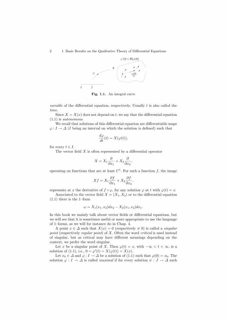
2 1 Basic Results on the Qualitative Theory of Differential Equations
∆
ϕ�(t) = X(ϕ(t))
ϕ(t)ϕ
tI
Fig. 1.1. An integral curve
variable of the differential equation, respectively. Usually t is also called thetime.
Since X = X(x) does not depend on t, we say that the differential equation(1.1) is autonomous.
We recall that solutions of this differential equation are differentiable mapsϕ : I → Δ (I being an interval on which the solution is defined) such that
dϕ
dt(t) = X(ϕ(t)),
for every t ∈ I.The vector field X is often represented by a differential operator
X = X1∂
∂x1+ X2
∂
∂x2,
operating on functions that are at least C1. For such a function f , the image
Xf = X1∂f
∂x1+ X2
∂f
∂x2,
represents at x the derivative of f ◦ ϕ, for any solution ϕ at t with ϕ(t) = x.Associated to the vector field X = (X1, X2) or to the differential equation
(1.1) there is the 1–form
ω = X1(x1, x2)dx2 − X2(x1, x2)dx1.
In this book we mainly talk about vector fields or differential equations, butwe will see that it is sometimes useful or more appropriate to use the languageof 1–forms, as we will for instance do in Chap. 4.
A point x ∈ Δ such that X(x) = 0 (respectively �= 0) is called a singularpoint (respectively regular point) of X. Often the word critical is used insteadof singular, but as critical may have different meanings depending on thecontext, we prefer the word singular.
Let x be a singular point of X. Then ϕ(t) = x, with −∞ < t < ∞, is asolution of (1.1), i.e., 0 = ϕ′(t) = X(ϕ(t)) = X(x).
Let x0 ∈ Δ and ϕ : I → Δ be a solution of (1.1) such that ϕ(0) = x0. Thesolution ϕ : I → Δ is called maximal if for every solution ψ : J → Δ such
1.1 Vector Fields and Flows 3
that I ⊂ J and ϕ = ψ|I then I = J and, consequently ϕ = ψ. In this case wewrite I = Ix0
and call it the maximal interval.Let ϕ : Ix0
→ Δ be a maximal solution; it can be regular or constant. Itsimage γϕ = {ϕ(t) : t ∈ Ix0
} ⊂ Δ endowed with the orientation induced by ϕ,in case ϕ is regular, is called the trajectory, orbit or (maximal) integral curveassociated to the maximal solution ϕ.
We recall that for a solution defining an integral curve the tangent vectorϕ′(t) at ϕ(t) coincides with the value of the vector field X at the point ϕ(t);see Fig. 1.1.
Theorem 1.1 Let X be a vector field of class Cr with 1 ≤ r ≤ +∞ or r = ω.Then the following statements hold.
(i) (Existence and uniqueness of maximal solutions). For every x ∈ Δ thereexists an open interval Ix on which a unique maximal solution ϕx of (1.1)is defined and satisfies the condition ϕx(0) = x.
(ii) (Flow properties). If y = ϕx(t) and t ∈ Ix, then Iy = Ix − t = {r− t : r ∈Ix} and ϕy(s) = ϕx(t + s) for every s ∈ Iy.
(iii) (Continuity with respect to initial conditions). Let Ω = {(t, x) : x ∈Δ, t ∈ Ix}. Then Ω is an open set in R3 and ϕ : Ω → R2 given byϕ(t, x) = ϕx(t) is a map of class Cr. Moreover, ϕ satisfies
D1D2ϕ(t, x) = DX(ϕ(t, x))D2ϕ(t, x)
for every (t, x) ∈ Ω where D1 denotes the derivative with respect to time,D2 denotes the derivative with respect to x, and DX denotes the linearpart of the vector field.
The proof of this theorem (and the others in this chapter) is given in [152]and [151]. We can also refer to [44].
We denote by ϕ : Ω → R2 the flow generated by the vector field X.It is clear that if Ix = R for every x, the flow generated by X is a flow
defined on Ω = R × Δ. But many times one has Ix �= R. For this reasonthe flow generated by X is often called the local flow generated by X. In caseΩ = R × R2, condition (ii) of Theorem 1.1 defines a group homomorphismt → ϕt from the additive group of the reals to the group of Cr diffeomorphismsfrom R2 to R2, endowed with the operation of composition. In case Δ �= R2
or Ix �= R the homomorphism property, expressed by condition (ii), holdsonly when the composition makes sense, inducing the word “local” in thedenomination. The name “flow” comes from the fact that points followingtrajectories of X resemble liquid particles following a laminar motion.
Theorem 1.2 Let X be a vector field of class Cr with 1 ≤ r ≤ +∞ or r = ω,and Δ ⊂ R2. Let x ∈ Δ and Ix = (ω−(x), ω+(x)) be such that ω+(x) < ∞(respectively ω−(x) > −∞). Then ϕx(t) tends to ∂Δ (the boundary of Δ)as t → ω+(x) (respectively t → ω−(x)), that is, for every compact K ⊂ Δthere exists ε = ε(K) > 0 such that if t ∈ [ω+(x) − ε, ω+(x)) (respectivelyt ∈ (ω−(x), ω−(x) + ε]), then ϕx(t) /∈ K.
4 1 Basic Results on the Qualitative Theory of Differential Equations
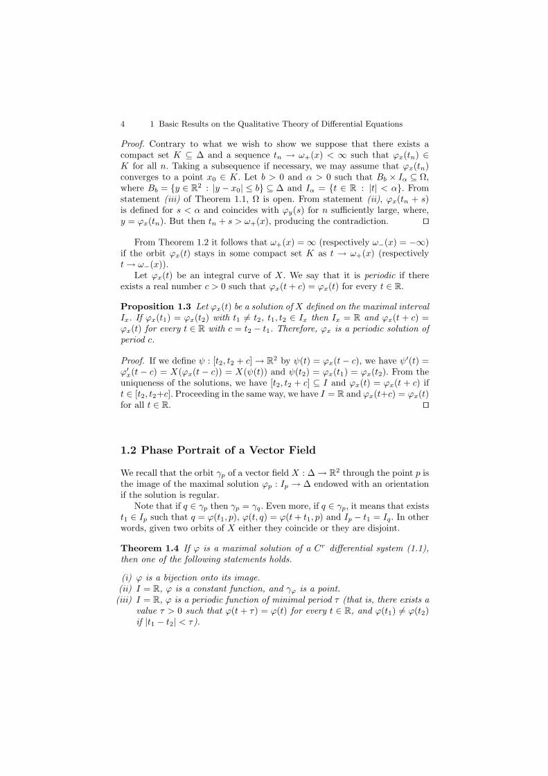
Proof. Contrary to what we wish to show we suppose that there exists acompact set K ⊆ Δ and a sequence tn → ω+(x) < ∞ such that ϕx(tn) ∈K for all n. Taking a subsequence if necessary, we may assume that ϕx(tn)converges to a point x0 ∈ K. Let b > 0 and α > 0 such that Bb × Iα ⊆ Ω,where Bb = {y ∈ R2 : |y − x0| ≤ b} ⊆ Δ and Iα = {t ∈ R : |t| < α}. Fromstatement (iii) of Theorem 1.1, Ω is open. From statement (ii), ϕx(tn + s)is defined for s < α and coincides with ϕy(s) for n sufficiently large, where,y = ϕx(tn). But then tn + s > ω+(x), producing the contradiction. ⊓⊔
From Theorem 1.2 it follows that ω+(x) = ∞ (respectively ω−(x) = −∞)if the orbit ϕx(t) stays in some compact set K as t → ω+(x) (respectivelyt → ω−(x)).
Let ϕx(t) be an integral curve of X. We say that it is periodic if thereexists a real number c > 0 such that ϕx(t + c) = ϕx(t) for every t ∈ R.
Proposition 1.3 Let ϕx(t) be a solution of X defined on the maximal intervalIx. If ϕx(t1) = ϕx(t2) with t1 �= t2, t1, t2 ∈ Ix then Ix = R and ϕx(t + c) =ϕx(t) for every t ∈ R with c = t2 − t1. Therefore, ϕx is a periodic solution ofperiod c.
Proof. If we define ψ : [t2, t2 + c] → R2 by ψ(t) = ϕx(t − c), we have ψ′(t) =ϕ′
x(t − c) = X(ϕx(t − c)) = X(ψ(t)) and ψ(t2) = ϕx(t1) = ϕx(t2). From theuniqueness of the solutions, we have [t2, t2 + c] ⊆ I and ϕx(t) = ϕx(t + c) ift ∈ [t2, t2+c]. Proceeding in the same way, we have I = R and ϕx(t+c) = ϕx(t)for all t ∈ R. ⊓⊔
1.2 Phase Portrait of a Vector Field
We recall that the orbit γp of a vector field X : Δ → R2 through the point p isthe image of the maximal solution ϕp : Ip → Δ endowed with an orientationif the solution is regular.
Note that if q ∈ γp then γp = γq. Even more, if q ∈ γp, it means that existst1 ∈ Ip such that q = ϕ(t1, p), ϕ(t, q) = ϕ(t + t1, p) and Ip − t1 = Iq. In otherwords, given two orbits of X either they coincide or they are disjoint.
Theorem 1.4 If ϕ is a maximal solution of a Cr differential system (1.1),then one of the following statements holds.
(i) ϕ is a bijection onto its image.(ii) I = R, ϕ is a constant function, and γϕ is a point.(iii) I = R, ϕ is a periodic function of minimal period τ (that is, there exists a
value τ > 0 such that ϕ(t + τ) = ϕ(t) for every t ∈ R, and ϕ(t1) �= ϕ(t2)if |t1 − t2| < τ).
1.2 Phase Portrait of a Vector Field 5
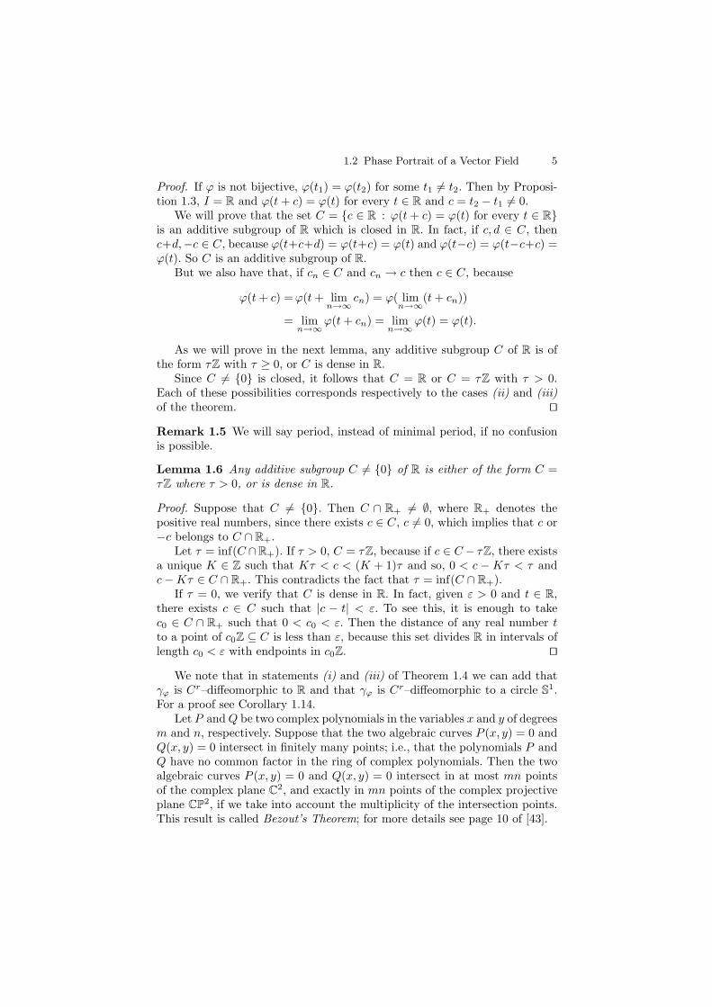
Proof. If ϕ is not bijective, ϕ(t1) = ϕ(t2) for some t1 �= t2. Then by Proposi-tion 1.3, I = R and ϕ(t + c) = ϕ(t) for every t ∈ R and c = t2 − t1 �= 0.
We will prove that the set C = {c ∈ R : ϕ(t + c) = ϕ(t) for every t ∈ R}is an additive subgroup of R which is closed in R. In fact, if c, d ∈ C, thenc+d,−c ∈ C, because ϕ(t+c+d) = ϕ(t+c) = ϕ(t) and ϕ(t−c) = ϕ(t−c+c) =ϕ(t). So C is an additive subgroup of R.
But we also have that, if cn ∈ C and cn → c then c ∈ C, because
ϕ(t + c) =ϕ(t + limn→∞
cn) = ϕ( limn→∞
(t + cn))
= limn→∞
ϕ(t + cn) = limn→∞
ϕ(t) = ϕ(t).
As we will prove in the next lemma, any additive subgroup C of R is ofthe form τZ with τ ≥ 0, or C is dense in R.
Since C �= {0} is closed, it follows that C = R or C = τZ with τ > 0.Each of these possibilities corresponds respectively to the cases (ii) and (iii)of the theorem. ⊓⊔
Remark 1.5 We will say period, instead of minimal period, if no confusionis possible.
Lemma 1.6 Any additive subgroup C �= {0} of R is either of the form C =τZ where τ > 0, or is dense in R.
Proof. Suppose that C �= {0}. Then C ∩ R+ �= ∅, where R+ denotes thepositive real numbers, since there exists c ∈ C, c �= 0, which implies that c or−c belongs to C ∩ R+.
Let τ = inf(C ∩R+). If τ > 0, C = τZ, because if c ∈ C − τZ, there existsa unique K ∈ Z such that Kτ < c < (K + 1)τ and so, 0 < c − Kτ < τ andc − Kτ ∈ C ∩ R+. This contradicts the fact that τ = inf(C ∩ R+).
If τ = 0, we verify that C is dense in R. In fact, given ε > 0 and t ∈ R,there exists c ∈ C such that |c − t| < ε. To see this, it is enough to takec0 ∈ C ∩ R+ such that 0 < c0 < ε. Then the distance of any real number tto a point of c0Z ⊆ C is less than ε, because this set divides R in intervals oflength c0 < ε with endpoints in c0Z. ⊓⊔
We note that in statements (i) and (iii) of Theorem 1.4 we can add thatγϕ is Cr–diffeomorphic to R and that γϕ is Cr–diffeomorphic to a circle S1.For a proof see Corollary 1.14.
Let P and Q be two complex polynomials in the variables x and y of degreesm and n, respectively. Suppose that the two algebraic curves P (x, y) = 0 andQ(x, y) = 0 intersect in finitely many points; i.e., that the polynomials P andQ have no common factor in the ring of complex polynomials. Then the twoalgebraic curves P (x, y) = 0 and Q(x, y) = 0 intersect in at most mn pointsof the complex plane C2, and exactly in mn points of the complex projectiveplane CP2, if we take into account the multiplicity of the intersection points.This result is called Bezout’s Theorem; for more details see page 10 of [43].
6 1 Basic Results on the Qualitative Theory of Differential Equations
A differential system of the form
x = P (x, y), y = Q(x, y),
where P and Q are polynomials in the real variables x and y is called apolynomial differential system of degree m if m is the maximum degree of thepolynomials P and Q.
From Bezout’s Theorem it follows that a polynomial differential systemof degree m has either infinitely many singular points (i.e., a continuum ofsingularities), or at most m2 singular points in R2.
By a phase portrait of the vector field X : Δ → R2 we mean the set of(oriented) orbits of X. It consists of singularities and regular orbits, orientedaccording to the maximal solutions describing them, hence in the sense ofincreasing t. In general, the phase portrait is represented by drawing a numberof significant orbits, representing the orientation (in case of regular orbits) byarrows. In Sect. 1.9 we will see how to look for a set of significant orbits.
Now we consider some examples.
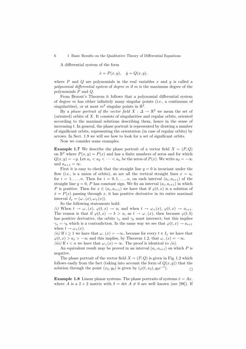
Example 1.7 We describe the phase portrait of a vector field X = (P,Q)on R2 where P (x, y) = P (x) and has a finite numbers of zeros and for whichQ(x, y) = −y. Let a1 < a2 < · · · < an be the zeros of P (x). We write a0 = −∞and an+1 = ∞.
First it is easy to check that the straight line y = 0 is invariant under theflow (i.e., is a union of orbits), as are all the vertical straight lines x = ai
for i = 1, . . . , n. Then for i = 0, 1, . . . , n, on each interval (ai, ai+1) of thestraight line y = 0, P has constant sign. We fix an interval (ai, ai+1) in whichP is positive. Then for x ∈ (ai, ai+1) we have that if ϕ(t, x) is a solution ofx = P (x) passing through x, it has positive derivative in its entire maximalinterval Ix = (ω−(x), ω+(x)).
So the following statements hold:(i) When t → ω−(x), ϕ(t, x) → ai and when t → ω+(x), ϕ(t, x) → ai+1.The reason is that if ϕ(t, x) → b > ai as t → ω−(x), then because ϕ(t, b)has positive derivative, the orbits γx and γb must intersect; but this impliesγx = γb which is a contradiction. In the same way we see that ϕ(t, x) → ai+1
when t → ω+(x).(ii) If i ≥ 1 we have that ω−(x) = −∞, because for every t ∈ Ix we have thatϕ(t, x) > a1 > −∞ and this implies, by Theorem 1.2, that ω−(x) = −∞.(iii) If i < n we have that ω+(x) = ∞. The proof is identical to (ii).
An equivalent result may be proved in an interval (ai, ai+1) on which P isnegative.
The phase portrait of the vector field X = (P,Q) is given in Fig. 1.2 whichfollows easily from the fact (taking into account the form of Q(x, y)) that thesolution through the point (x0, y0) is given by (ϕ(t, x0), y0e
−t).
Example 1.8 Linear planar systems. The phase portraits of systems x = Ax,where A is a 2 × 2 matrix with δ = det A �= 0 are well–known (see [98]). If
1.2 Phase Portrait of a Vector Field 7
a1a2 a3
a4a5
a1
a2 a3a4 a5
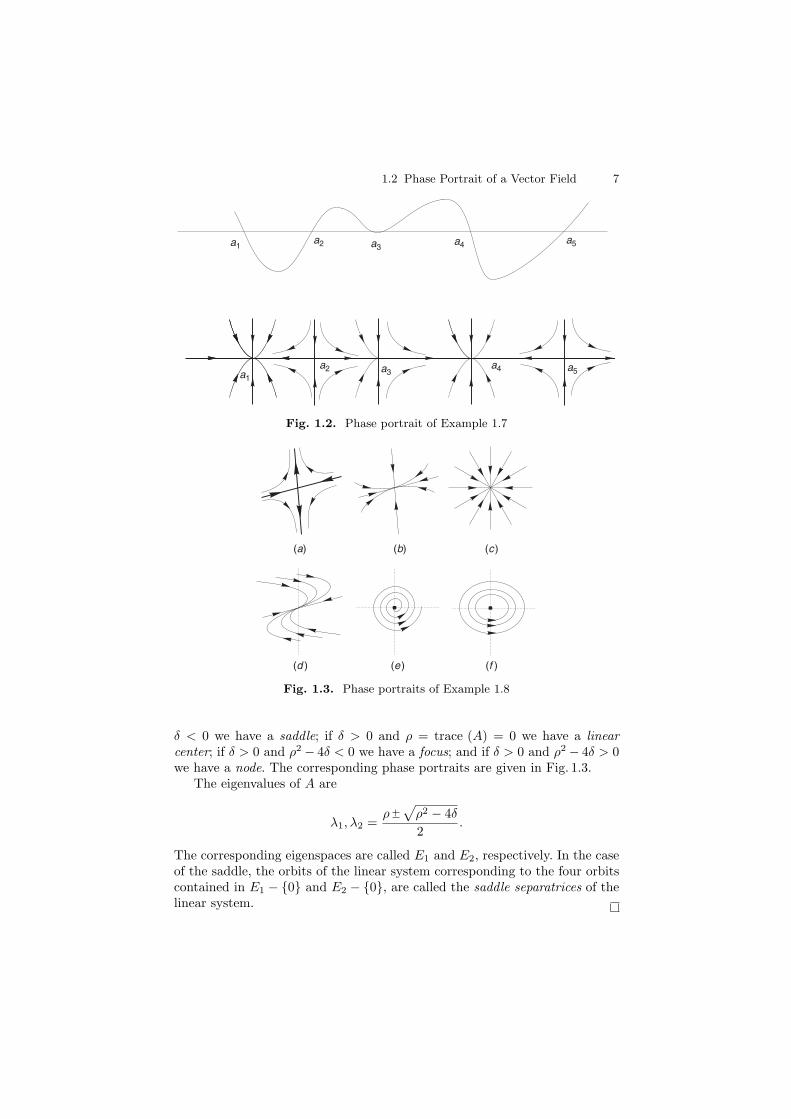
Fig. 1.2. Phase portrait of Example 1.7
(a) (b) (c )
(d ) (e ) (f )
Fig. 1.3. Phase portraits of Example 1.8
δ < 0 we have a saddle; if δ > 0 and ρ = trace (A) = 0 we have a linearcenter; if δ > 0 and ρ2 − 4δ < 0 we have a focus; and if δ > 0 and ρ2 − 4δ > 0we have a node. The corresponding phase portraits are given in Fig. 1.3.
The eigenvalues of A are
λ1, λ2 =ρ√
ρ2 − 4δ
2.
The corresponding eigenspaces are called E1 and E2, respectively. In the caseof the saddle, the orbits of the linear system corresponding to the four orbitscontained in E1 − {0} and E2 − {0}, are called the saddle separatrices of thelinear system.
8 1 Basic Results on the Qualitative Theory of Differential Equations
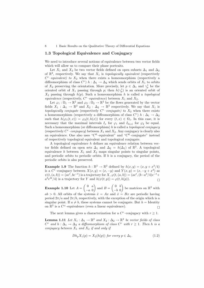
1.3 Topological Equivalence and Conjugacy
We need to introduce several notions of equivalence between two vector fieldswhich will allow us to compare their phase portraits.
Let X1 and X2 be two vector fields defined on open subsets Δ1 and Δ2
of R2, respectively. We say that X1 is topologically equivalent (respectivelyCr–equivalent) to X2 when there exists a homeomorphism (respectively adiffeomorphism of class Cr) h : Δ1 → Δ2 which sends orbits of X1 to orbitsof X2 preserving the orientation. More precisely, let p ∈ Δ1 and γ1
p be theoriented orbit of X1 passing through p; then h(γ1
p) is an oriented orbit ofX2 passing through h(p). Such a homeomorphism h is called a topologicalequivalence (respectively, Cr–equivalence) between X1 and X2.
Let ϕ1 : Ω1 → R2 and ϕ2 : Ω2 → R2 be the flows generated by the vectorfields X1 : Δ1 → R2 and X2 : Δ2 → R2 respectively. We say that X1 istopologically conjugate (respectively Cr–conjugate) to X2 when there existsa homeomorphism (respectively a diffeomorphism of class Cr) h : Δ1 → Δ2
such that h(ϕ1(t, x)) = ϕ2(t, h(x)) for every (t, x) ∈ Ω1. In this case, it isnecessary that the maximal intervals Ix for ϕ1 and Ih(x) for ϕ2 be equal.Such a homeomorphism (or diffeomorphism) h is called a topological conjugacy(respectively Cr–conjugacy) between X1 and X2. Any conjugacy is clearly alsoan equivalence. One also uses “C0–equivalent” and “C0–conjugate” insteadof respectively topological equivalent and topological conjugate.
A topological equivalence h defines an equivalence relation between vec-tor fields defined on open sets Δ1 and Δ2 = h(Δ1) of R2. A topologicalequivalence h between X1 and X2 maps singular points to singular points,and periodic orbits to periodic orbits. If h is a conjugacy, the period of theperiodic orbits is also preserved.
Example 1.9 The function h : R2 → R2 defined by h(x, y) = (x, y + x3/4)is a Cr–conjugacy between X(x, y) = (x,−y) and Y (x, y) = (x,−y + x3) asψ(t, (a, b)) = (aet, be−t) is a trajectory for X, ϕ(t, (a, b)) = (aet, (b−a3/4)e−t+a3e3t/4) is a trajectory for Y and h(ψ(t, p)) = ϕ(t, h(p)).
Example 1.10 Let A =
(0 a−a 0
)and B =
(0 b−b 0
)be matrices on R2 with
ab > 0. All orbits of the systems x = Ax and x = Bx are periodic havingperiod 2π/a and 2π/b, respectively, with the exception of the origin which is asingular point. If a �= b, these systems cannot be conjugate. But h = Identityon R2 is a Cω–equivalence (even a linear equivalence).
The next lemma gives a characterization for a Cr–conjugacy with r ≥ 1.
Lemma 1.11 Let X1 : Δ1 → R2 and X2 : Δ2 → R2 be vector fields of classCr and h : Δ1 → Δ2 a diffeomorphism of class Cr with r ≥ 1. Then h is aconjugacy between X1 and X2 if and only if
DhpX1(p) = X2(h(p)) for every p ∈ Δ1. (1.2)

1.3 Topological Equivalence and Conjugacy 9
Proof. Let ϕ1 : Ω1 → Δ1 and ϕ2 : Ω2 → Δ2 be the flows of X1 and X2,respectively. Assume that h satisfies (1.2). Given p ∈ Δ1, let ψ(t) = h(ϕ1(t, p))with t ∈ I1(p). Then ψ is a solution of x = X2(x), x(0) = h(p), because
ψ(t) =Dh(ϕ1(t, p))d
dtϕ1(t, p) = Dh(ϕ1(t, p))X1(ϕ1(t, p)) =
=X2(h(ϕ1(t, p))) = X2(ψ(t)).
So h(ϕ1(t, p)) = ϕ2(t, h(p)). Conversely, assume that h is a conjugacy. Givenp ∈ Δ1, we have that h(ϕ1(t, p)) = ϕ2(t, h(p)), t ∈ I1(p) = I2(h(p)). If wedifferentiate this relation with respect to t and evaluate at t = 0, we get(1.2). ⊓⊔
Let X : Δ → R2 be a vector field of class Cr and Δ ⊂ R2 and A ⊂ R opensubsets. A Cr map f : A → Δ is called a transverse local section of X whenfor every a ∈ A, f ′(a) and X(f(a)) are linearly independent. Take Σ = f(A)with the induced topology. If f : A → Σ is a homeomorphism (meaning thatf is an embedding) we say that Σ is a transverse section of X.
Theorem 1.12 (Flow Box Theorem) Let p be a regular point of a Cr vec-tor field X : Δ → R2 with 1 ≤ r ≤ +∞ or r = ω, and let f : A → Σ be atransverse section of X of class Cr with f(0) = p. Then there exists a neigh-borhood V of p in Δ and a diffeomorphism h : V → (−ε, ε) × B of class Cr,where ε > 0 and B is an open interval with center at the origin such that
(i) h(Σ ∩ V ) = {0} × B;(ii) h is a Cr–conjugacy between X|V and the constant vector field Y :
(−ε, ε) × B → R2 defined by Y = (1, 0). See Fig. 1.4.
Proof. Let ϕ : Ω → Δ be the flow of X. Let F : ΩA = {(t, u) : (t, f(u)) ∈Ω} → Δ be defined by F (t, u) = ϕ(t, f(u)). F maps parallel lines into integralcurves of X. We will prove that F is a local diffeomorphism in 0 = (0, 0) ∈R × R. By the Inverse Function Theorem, it is enough to prove that DF (0)is an isomorphism.
−ε ε
Σ
0
B∆
h
P
V
Fig. 1.4. The Flow Box Theorem
10 1 Basic Results on the Qualitative Theory of Differential Equations
We have that
D1F (0) =d
dtϕ(t, f(0)) |t=0 = X(ϕ(0, p)) = X(p),
and D2F (0) = D1f(0) because ϕ(0, f(u)) = f(u) for all u ∈ A. So the vectorsD1F (0) and D2F (0) generate R2 and DF (0) is an isomorphism.
By the Inverse Function Theorem, there exists ε > 0 and a neighborhood Bin R around the origin such that F |(−ε, ε)×B is a diffeomorphism on an openset V = F ((−ε, ε)×B). Let h = (F |(−ε, ε)×B)−1. Then h(Σ∩V ) = {0}×B,since F (0, u) = f(u) ∈ Σ for all u ∈ B. This proves (i). On the other hand,h−1 conjugates Y and X:
Dh−1(t, u)Y (t, u) = DF (t, u)(1, 0)
= D1F (t, u))
= X(ϕ(t, f(u)))
= X(F (t, u))
= X(h−1(t, u)),
for every (t, u) ∈ (−ε, ε) × B. This ends the proof. ⊓⊔
Corollary 1.13 Let Σ be a transverse section of X. For every point p ∈ Σ,there exist ε = ε(p) > 0, a neighborhood V of p in R2 and a function τ : V → R
of class Cr such that τ(V ∩ Σ) = 0 and:
(i) for every q ∈ V , an integral curve ϕ(t, q) of X|V is defined and bijectivein Jq = (−ε + τ(q), ε + τ(q)).
(ii) ξ(q) = ϕ(τ(q), q) ∈ Σ is the only point where ϕ(·, q)|Jq intersects Σ. Inparticular, q ∈ Σ ∩ V if and only if τ(q) = 0.
(iii) ξ : V → Σ is of class Cr and Dξ(q) is surjective for every q ∈ V . Evenmore, Dξ(q)v = 0 if and only if v = αX(q) for some α ∈ R.
Proof. Let h, V and ε be as in the Flow Box Theorem. We write h = (−τ, η).The vector field Y of that theorem satisfies all the statements of the corollary.Since h is a Cr–conjugacy, it follows that X also satisfies the statements. ⊓⊔
Corollary 1.14 If γ is a maximal solution of a Crdifferential system (1.1)and γ is not a singular point, then γ is Cr diffeomorphic to R or S1.
Proof. Let p be a point of γ. Let Σ be a transverse section of (1.1) suchthat p ∈ Σ ∩ γ. We define D = {t ∈ Ip : t ≥ 0, ϕ(t, p) ∈ Σ}. We claimthat taking Σ sufficiently small ϕ(t, p) with t ≥ 0 has a unique point onΣ. Indeed, because of the Flow Box Theorem, we know that D consists ofisolated points. If D �= {0}, let 0 and t0 be two consecutive elements of D.Now {ϕ(t, p) : t ∈ [0, t0]}, together with the segment of Σ in between ϕ(0) = pand ϕ(t0) = q, form a topological circle C, which by the Jordan’s CurveTheorem divides the plane in two connected components, like we represent inFig. 1.5(a) or (b). In both cases it is clear that the orbit through p cannot have

1.4 α- and ω-limit Sets of an Orbit 11
Σ
q
p
p
q
(a) (b)
or
Fig. 1.5. The arc {ϕ(t, p) : t ∈ [0, t0]}
other intersections with Σ, besides p, for Σ sufficiently small. So the claim isproved.
If in the arguments above p = q, then γ is a periodic orbit Cr diffeomorphicto S1. If p �= q, by the Flow Box Theorem applied again to this Σ, there is aneighborhood of p in γ which is Cr diffeomorphic to an open interval. Sincep is an arbitrary point of γ, it follows that γ is Cr diffeomorphic to R. ⊓⊔
Remark 1.15 The statement concerning regular periodic orbits is also validon surfaces in general and even in any dimension, but this is not the case forthe statement concerning regular non–periodic orbits.
1.4 α- and ω-limit Sets of an Orbit
Let Δ be an open subset of R2 and let X : Δ → R2 be a vector field of classCr where 1 ≤ r ≤ ∞ or r = ω.
Let ϕ(t) = ϕ(t, p) = ϕp(t) be the integral curve of X passing through thepoint p, defined on its maximal interval Ip = (ω−(p), ω+(p)). If ω+(p) = ∞we define the set
ω(p) = {q ∈ Δ : there exist {tn} with tn → ∞and ϕ(tn) → q when n → ∞}.
In the same way, if ω−(p) = −∞ we define the set
α(p) = {q ∈ Δ : there exist {tn} with tn → −∞and ϕ(tn) → q when n → ∞}.
The sets ω(p) and α(p) are called the ω-limit set (or simply ω-limit) and theα-limit set (or α-limit) of p, respectively.
We begin with some examples:
Example 1.16 Let X : R2 → R2 be a vector field given by X(x, y) = (x,−y).Then:
(i) If p = (0, 0), α(p) = ω(p) = {(0, 0)}.(ii) If p ∈ {(x, 0) : x �= 0}, α(p) = {(0, 0)} and ω(p) = ∅.
12 1 Basic Results on the Qualitative Theory of Differential Equations
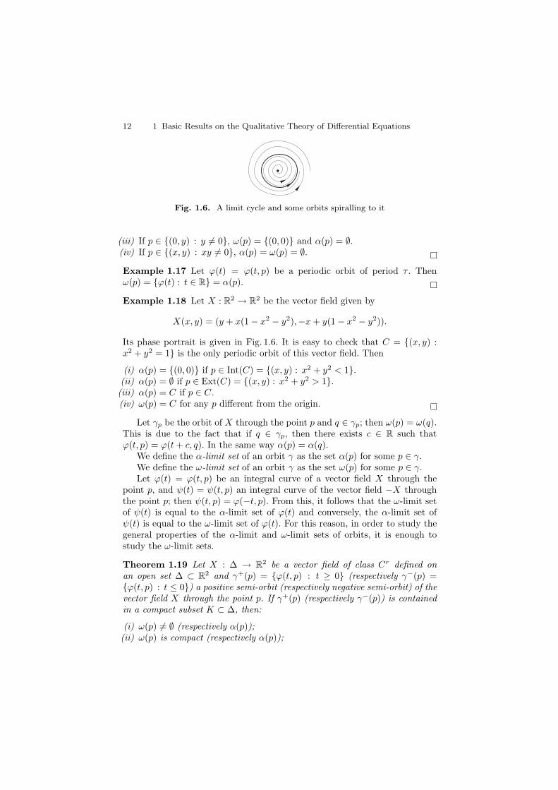
Fig. 1.6. A limit cycle and some orbits spiralling to it
(iii) If p ∈ {(0, y) : y �= 0}, ω(p) = {(0, 0)} and α(p) = ∅.(iv) If p ∈ {(x, y) : xy �= 0}, α(p) = ω(p) = ∅.
Example 1.17 Let ϕ(t) = ϕ(t, p) be a periodic orbit of period τ . Thenω(p) = {ϕ(t) : t ∈ R} = α(p).
Example 1.18 Let X : R2 → R2 be the vector field given by
X(x, y) = (y + x(1 − x2 − y2),−x + y(1 − x2 − y2)).
Its phase portrait is given in Fig. 1.6. It is easy to check that C = {(x, y) :x2 + y2 = 1} is the only periodic orbit of this vector field. Then
(i) α(p) = {(0, 0)} if p ∈ Int(C) = {(x, y) : x2 + y2 < 1}.(ii) α(p) = ∅ if p ∈ Ext(C) = {(x, y) : x2 + y2 > 1}.(iii) α(p) = C if p ∈ C.(iv) ω(p) = C for any p different from the origin.
Let γp be the orbit of X through the point p and q ∈ γp; then ω(p) = ω(q).This is due to the fact that if q ∈ γp, then there exists c ∈ R such thatϕ(t, p) = ϕ(t + c, q). In the same way α(p) = α(q).
We define the α-limit set of an orbit γ as the set α(p) for some p ∈ γ.We define the ω-limit set of an orbit γ as the set ω(p) for some p ∈ γ.Let ϕ(t) = ϕ(t, p) be an integral curve of a vector field X through the
point p, and ψ(t) = ψ(t, p) an integral curve of the vector field −X throughthe point p; then ψ(t, p) = ϕ(−t, p). From this, it follows that the ω-limit setof ψ(t) is equal to the α-limit set of ϕ(t) and conversely, the α-limit set ofψ(t) is equal to the ω-limit set of ϕ(t). For this reason, in order to study thegeneral properties of the α-limit and ω-limit sets of orbits, it is enough tostudy the ω-limit sets.
Theorem 1.19 Let X : Δ → R2 be a vector field of class Cr defined onan open set Δ ⊂ R2 and γ+(p) = {ϕ(t, p) : t ≥ 0} (respectively γ−(p) ={ϕ(t, p) : t ≤ 0}) a positive semi-orbit (respectively negative semi-orbit) of thevector field X through the point p. If γ+(p) (respectively γ−(p)) is containedin a compact subset K ⊂ Δ, then:
(i) ω(p) �= ∅ (respectively α(p));(ii) ω(p) is compact (respectively α(p));
1.4 α- and ω-limit Sets of an Orbit 13
(iii) ω(p) is invariant for X (respectively α(p)), that is, if q ∈ ω(p), then anintegral curve passing through q is contained in ω(p);
(iv) ω(p) is connected (respectively α(p)).(v) If ω(γ) ⊂ γ (respectively α(γ) ⊂ γ) then ω(γ) = γ (respectively α(γ) = γ),
and γ is either a singular point or a periodic orbit.
Proof. From the previous observation it is sufficient to prove the theorem fora set ω(p).
(i) ω(p) �= ∅.Let tn = n ∈ N. From the assumptions we have that {ϕ(tn)} ⊂ K with
K compact. Then there exists a subsequence {ϕ(tnk)} which converges to a
point q ∈ K. We have then that tnk→ ∞ as nk → ∞ and ϕ(tnk
) → q. Thenby definition q ∈ ω(p).
(ii) ω(p) is compact.We have that ω(p) ⊂ γ+(p) ⊂ K, so it is sufficient to prove that ω(p)
is closed. Let qn → q, with qn ∈ ω(p). We will prove that q ∈ ω(p). Since
qn ∈ ω(p), there exists for every qn a sequence {t(n)m } such that t
(n)m → ∞ and
ϕ(t(n)m , p) → qn as m → ∞.
For every sequence {t(n)m } we choose a point tn = t
(n)m(n) > n such that
d(ϕ(tn, p), qn) < 1/n. Then we have that:
d(ϕ(tn, p), q) ≤ d(ϕ(tn, p), qn) + d(qn, q) <1
n+ d(qn, q).
Therefore, it follows that d(ϕ(tn, p), q) → 0 as n → ∞, that is, ϕ(tn, p) →q. Since tn → ∞ as n → ∞, we get that q ∈ ω(p).
(iii) ω(p) is invariant under X.Let q ∈ ω(p) and let ψ : I(q) → Δ be an integral curve of X passing
through the point q. Let q1 = ϕ(t0, q) = ψ(t0). We will prove that q1 ∈ ω(p).As q ∈ ω(p), there exists a sequence {tn} such that tn → ∞ and ϕ(tn, p) → qas n → ∞. Since ϕ is continuous, it follows that:
q1 = ϕ(t0, q) = ϕ(t0, limn→∞
ϕ(tn, p))
= limn→∞
ϕ(t0, ϕ(tn, p)) = limn→∞
ϕ(t0 + tn, p).
We have then a sequence {sn} = {t0 + tn} such that sn → ∞ andϕ(sn, p) → q1 as n → ∞, that is q1 ∈ ω(p); see Fig. 1.7.
(iv) ω(p) is connected.Assume that ω(p) is not connected. Then ω(p) = A ∪ B, where A and B
are closed, non-empty and A ∩ B = ∅. As A �= ∅, there exists a subsequence{t′n} such that t′n → ∞ and ϕ(t′n) → a ∈ A as n → ∞. In the same way, thereexists a sequence {t′′n} such that t′′n → ∞ and ϕ(t′′n) → b ∈ B as n → ∞. Thenwe can construct a sequence {tn} such that tn → ∞ as n → ∞ and such thatd(ϕ(tn), A) < d/2 and d(ϕ(tn+1), A) > d/2, where d = d(A,B) > 0 for everyn odd.
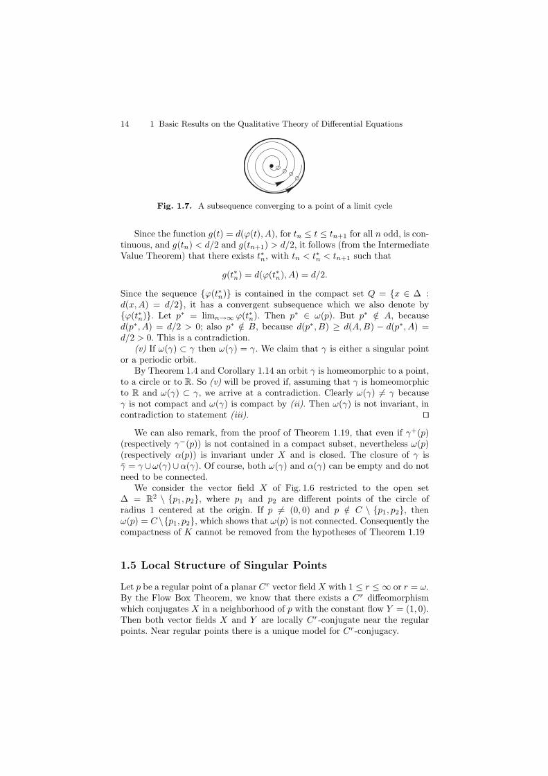
14 1 Basic Results on the Qualitative Theory of Differential Equations
Fig. 1.7. A subsequence converging to a point of a limit cycle
Since the function g(t) = d(ϕ(t), A), for tn ≤ t ≤ tn+1 for all n odd, is con-tinuous, and g(tn) < d/2 and g(tn+1) > d/2, it follows (from the IntermediateValue Theorem) that there exists t∗n, with tn < t∗n < tn+1 such that
g(t∗n) = d(ϕ(t∗n), A) = d/2.
Since the sequence {ϕ(t∗n)} is contained in the compact set Q = {x ∈ Δ :d(x,A) = d/2}, it has a convergent subsequence which we also denote by{ϕ(t∗n)}. Let p∗ = limn→∞ ϕ(t∗n). Then p∗ ∈ ω(p). But p∗ /∈ A, becaused(p∗, A) = d/2 > 0; also p∗ /∈ B, because d(p∗, B) ≥ d(A,B) − d(p∗, A) =d/2 > 0. This is a contradiction.
(v) If ω(γ) ⊂ γ then ω(γ) = γ. We claim that γ is either a singular pointor a periodic orbit.
By Theorem 1.4 and Corollary 1.14 an orbit γ is homeomorphic to a point,to a circle or to R. So (v) will be proved if, assuming that γ is homeomorphicto R and ω(γ) ⊂ γ, we arrive at a contradiction. Clearly ω(γ) �= γ becauseγ is not compact and ω(γ) is compact by (ii). Then ω(γ) is not invariant, incontradiction to statement (iii). ⊓⊔
We can also remark, from the proof of Theorem 1.19, that even if γ+(p)(respectively γ−(p)) is not contained in a compact subset, nevertheless ω(p)(respectively α(p)) is invariant under X and is closed. The closure of γ isγ = γ ∪ω(γ)∪α(γ). Of course, both ω(γ) and α(γ) can be empty and do notneed to be connected.
We consider the vector field X of Fig. 1.6 restricted to the open setΔ = R2 \ {p1, p2}, where p1 and p2 are different points of the circle ofradius 1 centered at the origin. If p �= (0, 0) and p /∈ C \ {p1, p2}, thenω(p) = C \{p1, p2}, which shows that ω(p) is not connected. Consequently thecompactness of K cannot be removed from the hypotheses of Theorem 1.19
1.5 Local Structure of Singular Points
Let p be a regular point of a planar Cr vector field X with 1 ≤ r ≤ ∞ or r = ω.By the Flow Box Theorem, we know that there exists a Cr diffeomorphismwhich conjugates X in a neighborhood of p with the constant flow Y = (1, 0).Then both vector fields X and Y are locally Cr-conjugate near the regularpoints. Near regular points there is a unique model for Cr-conjugacy.

1.5 Local Structure of Singular Points 15
Let p be a singular point of a planar Cr vector field X = (P,Q). In generalthe study of the local behavior of the flow near p is quite complicated. Alreadythe linear systems show different classes, even for local topological equivalence.We say that
DX(p) =
⎛⎜⎜⎜⎝
∂P
∂x(p)
∂P
∂y(p)
∂Q
∂x(p)
∂Q
∂y(p)
⎞⎟⎟⎟⎠
is the linear part of the vector field X at the singular point p.The singular point p is called non–degenerate if 0 is not an eigenvalue.The singular point p is called hyperbolic if the two eigenvalues of DX(p)
have real part different from 0.The singular point p is called semi-hyperbolic if exactly one eigenvalue of
DX(p) is equal to 0. Hyperbolic and semi-hyperbolic singularities are alsosaid to be elementary singular points.
The singular point p is called nilpotent if both eigenvalues of DX(p) areequal to 0 but DX(p) �≡ 0.
The singular point p is called linearly zero if DX(p) ≡ 0.The singular point p is called a center if there is an open neighborhood
consisting, besides the singularity, of periodic orbits. The singularity is said tobe linearly a center if the eigenvalues of DX(p) are purely imaginary withoutbeing zero. In that case, and if we suppose the vector field X to be analytic(see Chap. 4), the vector field X can have either a center or a focus at p.To distinguish between a center and a focus is a difficult problem in thequalitative theory of planar differential equations; see Chap. 4. We note thata center-focus problem also exists for nilpotent or linearly zero singular points.
In order to study the local phase portrait at the singular point p we definethe determinant, the trace and the discriminant at p as
det(p) =
∣∣∣∣∣∣∣∣∣
∂P
∂x(p)
∂P
∂y(p)
∂Q
∂x(p)
∂Q
∂y(p)
∣∣∣∣∣∣∣∣∣,
tr(p) =∂P
∂x(p) +
∂Q
∂y(p),
Δ(p) = tr(p)2 − 4det(p),
respectively. It is easy to check that
(i) if det(p) �= 0, then the singular point is non–degenerate and it is eitherhyperbolic, or linearly a center;
16 1 Basic Results on the Qualitative Theory of Differential Equations
(ii) if det(p) = 0 but tr(p) �= 0, then the singular point is semi-hyperbolic;(iii) if det(p) = 0 and tr(p) = 0, then the singular point is linearly zero or
nilpotent depending on whether DX(p) is the zero matrix or not.
It is obvious that if p = (x0, y0) is a singular point of the differential system
x = P (x, y),
y = Q(x, y),
then the point (0, 0) is a singular point of the system
˙x = P (x, y),
˙y = Q(x, y),(1.3)
where x = x + x0, and y = y + y0, and now the functions P (x, y) and Q(x, y)start with terms of order 1 in x and y. In other words, we can always move asingular point to the origin of coordinates in which case system (1.3) becomes(dropping the bars over x and y)
x = ax + by + F (x, y),
y = cx + dy + G(x, y),
where F and G vanish together with their first partial derivatives at (0, 0).By a linear change of coordinates the linearization DX(0, 0) regarded as thematrix (
a b
c d
),
can be placed in real Jordan canonical form.If the singularity is hyperbolic, the Jordan form is
(λ1 0
0 λ2
)or
(λ1 1
0 λ1
)or
(α β
−β α
)
with λ1λ2 �= 0, α �= 0 and β > 0.In the semi-hyperbolic case and the linearly center case, we obtain, respec-
tively (λ 0
0 0
)and
(0 β
−β 0
)
with λ �= 0 and β > 0, while we obtain
(0 1
0 0
)and
(0 0
0 0
)
in the nilpotent case and the linearly zero case, respectively.
1.5 Local Structure of Singular Points 17
If moreover we allow a time rescaling, introducing a new time u = γt forsome γ > 0, as is usual when working with equivalences, then we can alsosuppose that in the hyperbolic case one of the numbers λ1 or λ2 is equal to1 and either α = 1 or β = 1, while in the semi-hyperbolic case λ = 1 and
in the linearly center case β = 1.We are now going to study these different cases systematically.Let p be a singular point. A characteristic orbit γ(t) at p is an orbit tending
to p in positive time (respectively in negative time) with a well defined slope,i.e., γ(t) → p for t → ∞ (respectively t → −∞) and the limit limt→∞(γ(t) −p)/‖γ(t) − p‖ (respectively limt→−∞(γ(t) − p)/‖γ(t) − p‖) exists.
In Chap. 6 we will work along circles that can be obtained as the imageof an orientation preserving injective regular parametrization
ρ : S1 →R2
e2πit → ρ(e2πit)
with ρ of class C1, ρ′ �= 0 everywhere and ρ injective. We mean that thereexists some C1 functions Ψ : R → R2 with Ψ(t) = ρ(e2πit), Ψ|[0,1) injective,and such that Ψ′(t) = (Ψ′
1(t),Ψ′2(t)) �= 0 and n(t) = (−Ψ′
2(t),Ψ′1(t)) points
out of the (topological) disk encircled by ρ(S1). We can also write Ψ′(t) =ρ′(e2πit) and N(e2πit) = n(t); ρ′ and N are C0 functions on S1. We will callρ a permissible circle parametrization.
Let X be a C1 vector field defined in a compact neighborhood V of p, forwhich ∂V is the image of a C2 permissible circle parametrization ρ : S1 → ∂V ,and suppose that X(p) = 0 and X(q) �= 0 for all q ∈ V \ {p}.(i) We say that X|V is a center if ∂V is a periodic orbit and all orbits in
V \ {p} are periodic.(ii) We say that X|V is an attracting focus/node if at all points of ∂V the
vector field points inward and for all q ∈ V \ {p}, ω(q) = {p} and γ−(q)∩∂V �= ∅.
(iii) We say that X|V is a repelling focus/node if at all points of ∂V thevector field points outward and for all q ∈ V \ {p}, α(q) = {p} andγ+(q) ∩ ∂V �= ∅.
(iv) We say that X|V has a non-trivial finite sectorial decomposition if weare not in the case (i), (ii) or (iii) and if there exist a finite numberof characteristic orbits c0, . . . , cn−1, each cutting ∂V transversely at onepoint pi, in the sense that ∂V is a transverse section near pi, and withthe property that between ci and ci+1 (with cn = c0 and ordered in sucha way that p0, . . . , pn−1 follows the cyclic order of ρ), we have one of thefollowing situations with respect to the sector Si, defined as the compactregion bounded by {p}, ci, ci+1 and the piece of ∂V between pi and pi+1:(1) Attracting parabolic sector. At all points of [pi, pi+1] ⊂ ∂V the vector
field points inward, and for all q ∈ Si \ {p}, ω(q) = {p} and γ−(q) ∩∂V �= ∅.
18 1 Basic Results on the Qualitative Theory of Differential Equations
(2) Repelling parabolic sector. At all points of [pi, pi+1] ⊂ ∂V the vectorfield points outward, and for all q ∈ Si \ {p}, α(q) = {p} and γ+(q) ∩∂V �= ∅.
(3) Hyperbolic sector. There exists a point qi ∈ (pi, pi+1) ⊂ ∂V with theproperty that at all points of [pi, qi) the vector field points inward(respectively outward) while at all points of (qi, pi+1] the vector fieldpoints outward (respectively inward); at qi the vector field is tangentat ∂V and the tangency is external in the sense that the x–orbit of qi
stays outside V ; and for all q ∈ Si\ci ∪ ci+1 ∪ qi we have γ+(q)∩ ∂V �=∅ and γ−(q) ∩ ∂V �= ∅.
(4) Elliptic sector. There exists a point qi ∈ (pi, pi+1) ⊂ ∂V with theproperty that γ(qi) ⊂ V with ω(qi) = α(qi) = {p}; at all pointsq ∈ [pi, qi) the vector field points inward, γ+(q) ⊂ V and ω(q) = p.
We denote by S[pi,qi] =⋃
q∈[pi,qi]
γ+(q); at all points of q ∈ (qi, pi+1] the
vector field points outward, γ−(q) ⊂ V and α(q) = p. We denote by
S[qi,pi+1] =⋃
q∈[qi,pi+1]
γ−(q); at all points q of S\(S[pi,qi]∪S[qi,pi+1]∪{p})
we have γ(q) ⊂ V with ω(q) = α(q) = p.The same may also be true for [pi, qi] and [qi, pi+1] interchanged.
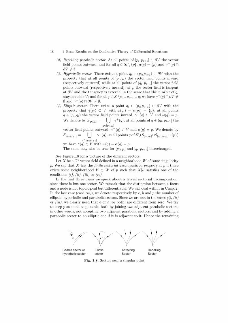
See Figure 1.8 for a picture of the different sectors.Let X be a C1 vector field defined in a neighborhood W of some singularity
p. We say that X has the finite sectorial decomposition property at p if thereexists some neighborhood V ⊂ W of p such that X|V satisfies one of theconditions (i), (ii), (iii) or (iv).
In the first three cases we speak about a trivial sectorial decomposition,since there is but one sector. We remark that the distinction between a focusand a node is not topological but differentiable. We will deal with it in Chap. 2.In the last case (case (iv)), we denote respectively by e, h and p the number ofelliptic, hyperbolic and parabolic sectors. Since we are not in the cases (i), (ii)or (iii), we clearly need that e or h, or both, are different from zero. We tryto keep p as small as possible, both by joining two adjacent parabolic sectors,in other words, not accepting two adjacent parabolic sectors, and by adding aparabolic sector to an elliptic one if it is adjacent to it. Hence the remaining
Saddle sector or hyperbolic sector
Ellipticsector
AttractingSector
RepellingSector
Fig. 1.8. Sectors near a singular point
1.5 Local Structure of Singular Points 19
parabolic sectors can only be the ones lying between two hyperbolic sectors.We call this a minimal sectorial decomposition.
Since X(pi) and X(pi+1) cannot both be pointing inward (or outward) ifSi is a hyperbolic or an elliptic sector, it is clear that e + h is always even.It is also clear that in a minimal non-trivial sectorial decomposition we havep ≤ h. For the sake of completeness we define (e, h) = (0, 0) in the cases (i),(ii) or (iii).
It is possible to define a more general notion of sectorial decompositionthat could be called “C0 finite sectorial decomposition” and that avoids thenotion of tangency. However, since we are interested in analytic vector fields,we do not need to do this. In the use of the finite sectorial decomposition,we will therefore not try to be as general as possible, but we will requirethe differentiability (the specific C1-class) which permits us to provide thesimplest proof.
In Chap. 3 we will show how to prove that every analytic vector field hasthe finite sectorial decomposition property at every isolated zero. The samedoes not necessarily hold for C∞ vector fields, but it does hold if we add theso called �Lojasiewicz condition (see Chap. 3). In both cases we will see thatthe permissible parametrization of the boundary ∂V can be taken as a C∞
mapping ρ : S1 → ∂V .For an oriented regular simple closed curve surrounding a point p, like a
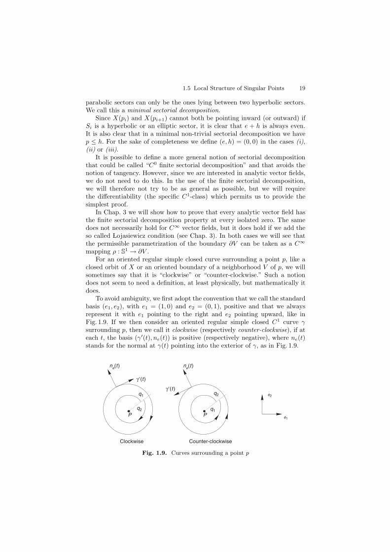
closed orbit of X or an oriented boundary of a neighborhood V of p, we willsometimes say that it is “clockwise” or “counter-clockwise.” Such a notiondoes not seem to need a definition, at least physically, but mathematically itdoes.
To avoid ambiguity, we first adopt the convention that we call the standardbasis (e1, e2), with e1 = (1, 0) and e2 = (0, 1), positive and that we alwaysrepresent it with e1 pointing to the right and e2 pointing upward, like inFig. 1.9. If we then consider an oriented regular simple closed C1 curve γsurrounding p, then we call it clockwise (respectively counter-clockwise), if ateach t, the basis (γ′(t), ne(t)) is positive (respectively negative), where ne(t)stands for the normal at γ(t) pointing into the exterior of γ, as in Fig. 1.9.
P P
q2 q1
q1q2
γ�(t )
γ�(t )
ne(t )n
e(t )
e2
e1
Counter-clockwiseClockwise
Fig. 1.9. Curves surrounding a point p
20 1 Basic Results on the Qualitative Theory of Differential Equations
Both notions easily extend to piecewise C1 oriented simple closed curvesas well as to curves γ that are not closed, but move from a point q1 �= p tosome q2 with −→pq2 = r(−→pq1), with r > 0, in a way that the closed curve formedby γ and −−→q2q1 is a piecewise C1 oriented simple closed curve surrounding p.
The permissible circle parametrizations, that we have used in the definitionof finite sectorial decomposition, turn in a clockwise way.
It can be proven that the topological equivalence classes for a given isolatedsingular point are characterized by the number of elliptic, hyperbolic andparabolic sectors (denoted by e, h, p, respectively) and the arrangement ofthese sectors. There also exist results describing which triples of non-negativeintegers (e, h, p) are possible and which arrangement can be realized for eachof these triples, depending on the minimal degree m of the singularity, which isthe lowest degree of the non-zero terms in the Taylor expansion of the vectorfield at the singular point. We state a theorem on the number of elliptic andhyperbolic sectors without giving a proof.
Theorem 1.20 Suppose that (e, h) is a couple of non-negative integers suchthat e+h > 0. Then there is a singular point of minimal degree m whose localphase portrait has e elliptic sectors and h hyperbolic sectors if and only if
(i) e + h ≡ 0 (mod 2);(ii) e ≤ 2m − 1 and e + h ≤ 2m + 2;(iii) if e �= 0, then e + h ≤ 2m.
There also exist results on the maximum number of parabolic sectors pdepending on m, e and h. For a precise description of such results and theirproofs see the bibliographical comments in Sect. 1.11.
We remark that Theorem 1.20 does not give any information about centersor foci, since then e+h = 0, but we have the well-known fact that the center-focus class is non-empty if and only if m is odd.
By using Theorem 1.20, we can easily get a finite list of pictures for anygiven m such that the local phase portrait of a singularity of a vector fieldof minimal degree m is topologically equivalent to one of them. To do this,it suffices to draw all possible minimal sectorial decompositions for any triple(e, h, p) with (e, h) satisfying Theorem 1.20 and p ≤ h. Notice that this listmay contain some pictures which cannot be realized.
1.6 Local Structure Near Periodic Orbits
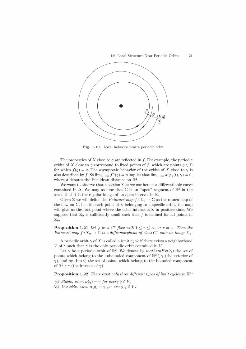
Let γ = {ϕp(t) : t ∈ R} be a periodic orbit of period τ0 of a vector field X ofclass Cr defined in an open subset Δ ⊂ R2, where r denotes a positive integer,+∞ or ω. Let Σ be a transverse section to X at p. Due to the continuity ofthe flow ϕ of X, for every point q ∈ Σ close to p, the trajectory ϕq(t) remainsclose to γ, with t in a given compact interval, for example, [0, 2τ0]. We definef(q) as the first point where ϕq(t) intersects Σ. Let Σ0 be the domain of f .Of course we have that p ∈ Σ0 and f(p) = p; see Fig. 1.10.
1.6 Local Structure Near Periodic Orbits 21
q(q)f
Σ
P
Fig. 1.10. Local behavior near a periodic orbit
The properties of X close to γ are reflected in f . For example, the periodicorbits of X close to γ correspond to fixed points of f , which are points q ∈ Σfor which f(q) = q. The asymptotic behavior of the orbits of X close to γ isalso described by f . So limn→∞ fn(q) = p implies that limt→∞ d(ϕq(t), γ) = 0,where d denotes the Euclidean distance on R2.
We want to observe that a section Σ as we use here is a differentiable curvecontained in Δ. We may assume that Σ is an “open” segment of R2 in thesense that it is the regular image of an open interval in R.
Given Σ we will define the Poincare map f : Σ0 → Σ as the return map ofthe flow on Σ, i.e., for each point of Σ belonging to a specific orbit, the mapwill give us the first point where the orbit intersects Σ in positive time. Wesuppose that Σ0 is sufficiently small such that f is defined for all points inΣ0,
Proposition 1.21 Let ϕ be a Cr-flow with 1 ≤ r ≤ ∞ or r = ω. Then thePoincare map f : Σ0 → Σ is a diffeomorphism of class Cr onto its image Σ1.
A periodic orbit γ of X is called a limit cycle if there exists a neighborhoodV of γ such that γ is the only periodic orbit contained in V .
Let γ be a periodic orbit of R2. We denote by mathrmExt(γ) the set ofpoints which belong to the unbounded component of R2 \ γ (the exterior ofγ), and by Int(γ) the set of points which belong to the bounded componentof R2 \ γ (the interior of γ).
Proposition 1.22 There exist only three different types of limit cycles in R2:
(i) Stable, when ω(q) = γ for every q ∈ V ;(ii) Unstable, when α(q) = γ for every q ∈ V ;

22 1 Basic Results on the Qualitative Theory of Differential Equations
(iii) Semi-stable, when ω(q) = γ for every q ∈ V ∩ Ext(γ) and α(q) = γ forevery q ∈ V ∩ Int(γ), or conversely.
We see that γ is a limit cycle if and only if p is an isolated fixed point off . Moreover,
(i) γ is stable if and only if |f(x) − p| < |x − p| for every x �= p sufficientlyclose to p;
(ii) γ is unstable if and only if |f(x)− p| > |x− p| for every x �= p sufficientlyclose to p;
(iii) γ is semi-stable if and only if |f(x)−p| < |x−p| for every x ∈ Σ∩ Ext (γ),x �= p sufficiently close to p, and |f(x) − p| < |x − p| for every x ∈Σ ∩ Int (γ), x �= p sufficiently close to p, or conversely.
In particular, if X is analytic and f(x) is not the identity, then f(x) =x + ak(x − p)k + · · · with ak �= 0. So if k is odd, then γ is stable if ak < 0,and unstable if ak > 0. If k is even, then γ is semi-stable. If f(x) ≡ x, thenall ak are zero and γ lies in the interior of an annulus of periodic orbits of X,that is, it is not a limit cycle.
If f ′(p) < 1 then we can apply the Intermediate Value Theorem anddeduce that γ is stable. Equivalently, γ is unstable if f ′(p) > 1; see Fig. 1.11.We remark that f ′(p) > 0, because a Poincare map on the plane is orientationpreserving. It is easy to see that f ′(p) is independent of the chosen regularparameter x on Σ as well as on p ∈ γ; it is called the characteristic exponentof γ.
In what follows we shall study the Poincare map for a differential equationin the plane. We consider a differential equation in the plane given by
x = P (x, y),
y = Q(x, y).
Let X(x, y) = (P (x, y), Q(x, y)) be the corresponding vector field. Denote thedivergence of X at q by (divX)(q). Assume that Σ is a transverse section andΣ′ ⊂ Σ is an open subset on which the Poincare map is defined, f : Σ′ → Σ.
Fig. 1.11. Different classes of limit cycles and their Poincare maps

1.6 Local Structure Near Periodic Orbits 23
Since the differential equations are in the plane, Σ is a curve which can beparametrized by γ : I → Σ with γ(I ′) = Σ′ and |γ′(s)| = 1. Let X⊥(q) be thescalar component to the tangent line to Σ at q given by
X⊥ ◦ γ(s) = det(γ′(s), X ◦ γ(s)).
In the case that Σ is a horizontal line, {(x, y∗) : x1 < x < x2}, X⊥(q) = Q(q).In the case that Σ is an vertical line, {(x∗, y) : y1 < y < y2}, X⊥(q) = P (q).
Let τ(q) be the return time for q ∈ Σ′, so f(p) = ϕτ(q)(q) = ϕq(τ(q)).The next theorem gives a sufficient condition for determining the stability
of a limit cycle.
Theorem 1.23 Let γ : I ′ → Σ′ be a parametrization of the transverse sectionΣ′ as above with |γ′(s)| = 1. Then for s ∈ I ′,
(γ−1 ◦ f ◦ γ)′(s) =X⊥ ◦ γ(s)
X⊥ ◦ f ◦ γ(s)exp
(∫ τ◦γ(s)
0
(divX) ◦ ϕt ◦ γ(s) dt
).
Thus if f(p) = p and γ(s0) = p, then the characteristic exponent of γ isgiven by
f ′(p) = (γ−1 ◦ f ◦ γ)′(s0) = exp
(∫ τ(p)
0
(divX) ◦ ϕt(p) dt
).
Proof. The first variational equation states that
d
dtDϕt
q = DXϕt(q)Dϕtq.
Since det(Dϕ0q) = det(id) = 1, Liouville’s formula for time-dependent linear
equations gives
det(Dϕτ(q)q ) = exp
(∫ τ(q)
0
(divX) ◦ ϕt(q) dt
).
Notice that the right-hand side of this equality is the exponential in the for-mula for (γ−1 ◦ f ◦ γ)′(s) as stated in the theorem. Therefore to complete the
proof, we must relate (γ−1 ◦ f ◦ γ)′(s) to det(Dϕτ◦γ(s)γ(s) ).
Taking the derivative of f ◦ γ(s) = ϕτ◦γ(s)(γ(s)) with respect to s yields
(f ◦ γ)′(s) = (Dϕτ◦γ(s)γ(s) )γ′(s) + (τ ◦ γ)′(s)[X ◦ ϕτ◦γ(s)(γ(s))]
= (Dϕτ◦γ(s)γ(s) )γ′(s) + (τ ◦ γ)′(s)[X ◦ f ◦ γ(s)].
24 1 Basic Results on the Qualitative Theory of Differential Equations
Then
(γ−1 ◦ f ◦ γ)′(s)[X⊥ ◦ f ◦ γ(s)] = det((f ◦ γ)′(s), X ◦ f ◦ γ(s))
= det((Dϕτ◦γ(s)γ(s) )γ′(s), X ◦ f ◦ γ(s))
+ det((τ ◦ γ)′(s)[X ◦ f ◦ γ(s)], X ◦ f ◦ γ(s))
= det((Dϕτ◦γ(s)γ(s) )γ′(s), (Dϕ
τ◦γ(s)γ(s) )X ◦ γ(s))
= det((Dϕτ◦γ(s)γ(s) )det(γ′(s), X ◦ γ(s))
= exp
(∫ τ◦γ(s)
0
(divX) ◦ ϕt ◦ γ(s) dt
)X⊥ ◦ γ(s).
Dividing by X⊥ ◦ f ◦ γ(s), the theorem is proved. ⊓⊔
Theorem 1.23 is contained in Sect. 28 of [4] or in Sect. 5.8.3 of [136].The following theorem provides another way to compute the stability of a
limit cycle. This result is due independently to Freire, Gasull and Guillamon[68] and to Chicone and Liu [34].
Theorem 1.24 Let γ be a τ0-periodic orbit of a C2 planar vector field X.Assume that in a neighborhood V of γ, X admits a transverse Lie symmetrygiven by the vector field Y , i.e., [Y,X] = μY . Let Σ = {ψ(p, s) : s ∈ R} ∩ V ,be a transverse section to γ, where ψ(p, s) is the solution of x = Y (x) withψ(p, 0) = p. Then the characteristic exponent of γ is given by
f ′(p) = exp
(∫ τ0
0
μ(γ(s)) ds
),
where f is the Poincare map on Σ.
1.7 The Poincare–Bendixson Theorem
In what follows, we are going to assume that Δ is an open subset of R2 andX is a vector field of class Cr with r ≥ 1. Also, in Δ, γ+
p denotes a positivesemi–orbit passing through the point p.
Theorem 1.25 (Poincare–Bendixson Theorem I) Let ϕ(t) = ϕ(t, p) bean integral curve of X defined for all t ≥ 0, such that γ+
p is contained ina compact set K ⊂ Δ. Assume that the vector field X has at most a finitenumber of singularities in K. Then one of the following statements holds.
(i) If ω(p) contains only regular points, then ω(p) is a periodic orbit.(ii) If ω(p) contains both regular and singular points, then ω(p) is formed by
a set of orbits, every one of which tends to one of the singular points inω(p) as t → ∞.
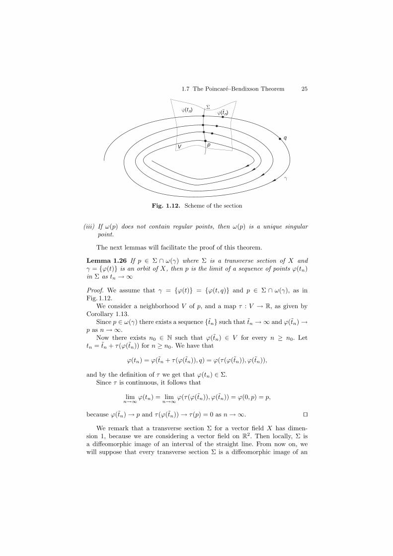
1.7 The Poincare–Bendixson Theorem 25
q
γ
Σ
pV
ϕ(tn)~ϕ(tn)
Fig. 1.12. Scheme of the section
(iii) If ω(p) does not contain regular points, then ω(p) is a unique singularpoint.
The next lemmas will facilitate the proof of this theorem.
Lemma 1.26 If p ∈ Σ ∩ ω(γ) where Σ is a transverse section of X andγ = {ϕ(t)} is an orbit of X, then p is the limit of a sequence of points ϕ(tn)in Σ as tn → ∞
Proof. We assume that γ = {ϕ(t)} = {ϕ(t, q)} and p ∈ Σ ∩ ω(γ), as inFig. 1.12.
We consider a neighborhood V of p, and a map τ : V → R, as given byCorollary 1.13.
Since p ∈ ω(γ) there exists a sequence {tn} such that tn → ∞ and ϕ(tn) →p as n → ∞.
Now there exists n0 ∈ N such that ϕ(tn) ∈ V for every n ≥ n0. Lettn = tn + τ(ϕ(tn)) for n ≥ n0. We have that
ϕ(tn) = ϕ(tn + τ(ϕ(tn)), q) = ϕ(τ(ϕ(tn)), ϕ(tn)),
and by the definition of τ we get that ϕ(tn) ∈ Σ.Since τ is continuous, it follows that
limn→∞
ϕ(tn) = limn→∞
ϕ(τ(ϕ(tn)), ϕ(tn)) = ϕ(0, p) = p,
because ϕ(tn) → p and τ(ϕ(tn)) → τ(p) = 0 as n → ∞. ⊓⊔
We remark that a transverse section Σ for a vector field X has dimen-sion 1, because we are considering a vector field on R2. Then locally, Σ isa diffeomorphic image of an interval of the straight line. From now on, wewill suppose that every transverse section Σ is a diffeomorphic image of an
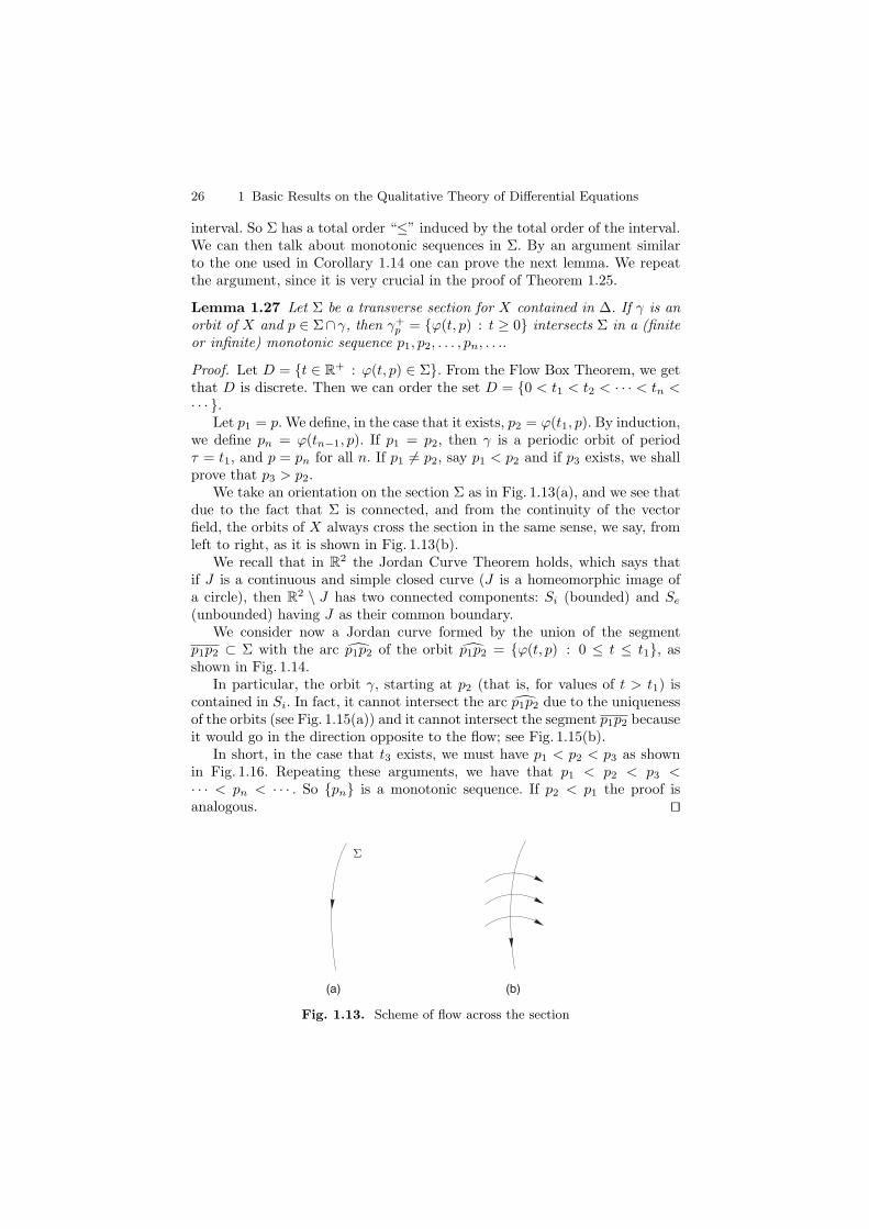
26 1 Basic Results on the Qualitative Theory of Differential Equations
interval. So Σ has a total order “≤” induced by the total order of the interval.We can then talk about monotonic sequences in Σ. By an argument similarto the one used in Corollary 1.14 one can prove the next lemma. We repeatthe argument, since it is very crucial in the proof of Theorem 1.25.
Lemma 1.27 Let Σ be a transverse section for X contained in Δ. If γ is anorbit of X and p ∈ Σ∩γ, then γ+
p = {ϕ(t, p) : t ≥ 0} intersects Σ in a (finiteor infinite) monotonic sequence p1, p2, . . . , pn, . . ..
Proof. Let D = {t ∈ R+ : ϕ(t, p) ∈ Σ}. From the Flow Box Theorem, we getthat D is discrete. Then we can order the set D = {0 < t1 < t2 < · · · < tn <· · · }.
Let p1 = p. We define, in the case that it exists, p2 = ϕ(t1, p). By induction,we define pn = ϕ(tn−1, p). If p1 = p2, then γ is a periodic orbit of periodτ = t1, and p = pn for all n. If p1 �= p2, say p1 < p2 and if p3 exists, we shallprove that p3 > p2.
We take an orientation on the section Σ as in Fig. 1.13(a), and we see thatdue to the fact that Σ is connected, and from the continuity of the vectorfield, the orbits of X always cross the section in the same sense, we say, fromleft to right, as it is shown in Fig. 1.13(b).
We recall that in R2 the Jordan Curve Theorem holds, which says thatif J is a continuous and simple closed curve (J is a homeomorphic image ofa circle), then R2 \ J has two connected components: Si (bounded) and Se
(unbounded) having J as their common boundary.We consider now a Jordan curve formed by the union of the segment
p1p2 ⊂ Σ with the arc p1p2 of the orbit p1p2 = {ϕ(t, p) : 0 ≤ t ≤ t1}, asshown in Fig. 1.14.
In particular, the orbit γ, starting at p2 (that is, for values of t > t1) iscontained in Si. In fact, it cannot intersect the arc p1p2 due to the uniquenessof the orbits (see Fig. 1.15(a)) and it cannot intersect the segment p1p2 becauseit would go in the direction opposite to the flow; see Fig. 1.15(b).
In short, in the case that t3 exists, we must have p1 < p2 < p3 as shownin Fig. 1.16. Repeating these arguments, we have that p1 < p2 < p3 <· · · < pn < · · · . So {pn} is a monotonic sequence. If p2 < p1 the proof isanalogous. ⊓⊔
(b)
Σ
(a)
Fig. 1.13. Scheme of flow across the section
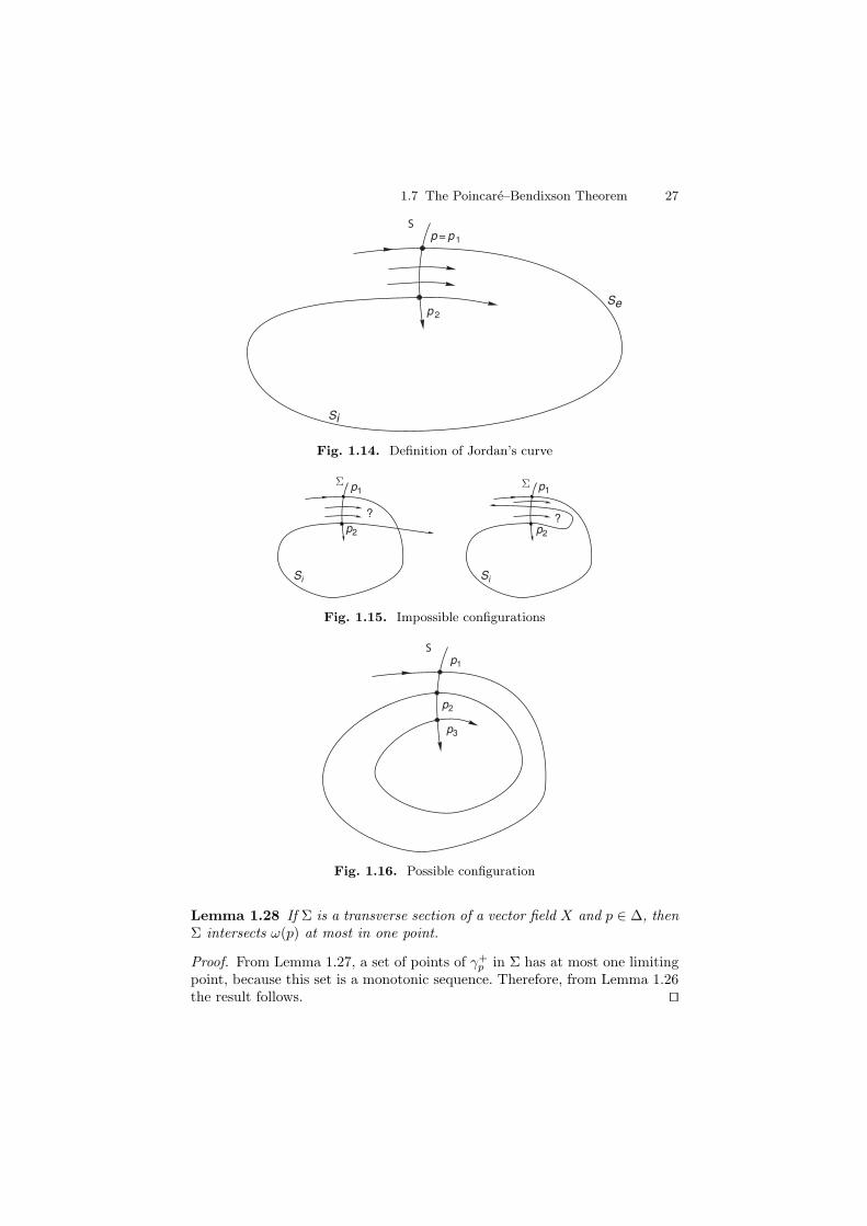
1.7 The Poincare–Bendixson Theorem 27
S
p2
p = p1
Si
Se
Fig. 1.14. Definition of Jordan’s curve
Σ Σ
Si Si
p1 p1
p2 p2
? ?
Fig. 1.15. Impossible configurations
S
p2
p1
p3
Fig. 1.16. Possible configuration
Lemma 1.28 If Σ is a transverse section of a vector field X and p ∈ Δ, thenΣ intersects ω(p) at most in one point.
Proof. From Lemma 1.27, a set of points of γ+p in Σ has at most one limiting
point, because this set is a monotonic sequence. Therefore, from Lemma 1.26the result follows. ⊓⊔
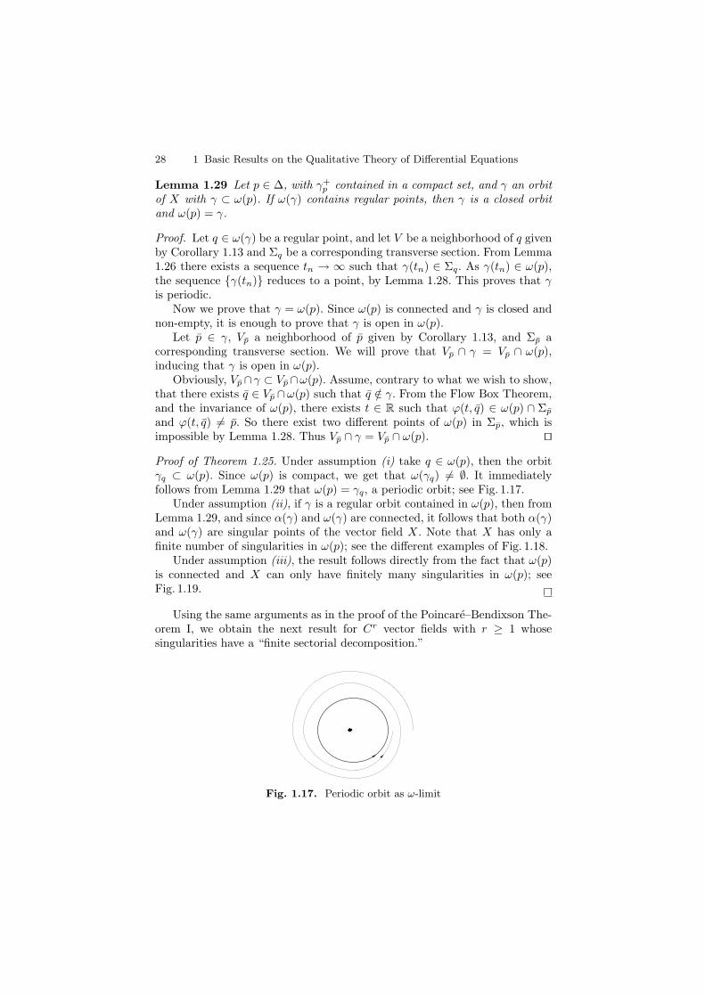
28 1 Basic Results on the Qualitative Theory of Differential Equations
Lemma 1.29 Let p ∈ Δ, with γ+p contained in a compact set, and γ an orbit
of X with γ ⊂ ω(p). If ω(γ) contains regular points, then γ is a closed orbitand ω(p) = γ.
Proof. Let q ∈ ω(γ) be a regular point, and let V be a neighborhood of q givenby Corollary 1.13 and Σq be a corresponding transverse section. From Lemma1.26 there exists a sequence tn → ∞ such that γ(tn) ∈ Σq. As γ(tn) ∈ ω(p),the sequence {γ(tn)} reduces to a point, by Lemma 1.28. This proves that γis periodic.
Now we prove that γ = ω(p). Since ω(p) is connected and γ is closed andnon-empty, it is enough to prove that γ is open in ω(p).
Let p ∈ γ, Vp a neighborhood of p given by Corollary 1.13, and Σp acorresponding transverse section. We will prove that Vp ∩ γ = Vp ∩ ω(p),inducing that γ is open in ω(p).
Obviously, Vp ∩γ ⊂ Vp ∩ω(p). Assume, contrary to what we wish to show,that there exists q ∈ Vp ∩ω(p) such that q /∈ γ. From the Flow Box Theorem,and the invariance of ω(p), there exists t ∈ R such that ϕ(t, q) ∈ ω(p) ∩ Σp
and ϕ(t, q) �= p. So there exist two different points of ω(p) in Σp, which isimpossible by Lemma 1.28. Thus Vp ∩ γ = Vp ∩ ω(p). ⊓⊔
Proof of Theorem 1.25. Under assumption (i) take q ∈ ω(p), then the orbitγq ⊂ ω(p). Since ω(p) is compact, we get that ω(γq) �= ∅. It immediatelyfollows from Lemma 1.29 that ω(p) = γq, a periodic orbit; see Fig. 1.17.
Under assumption (ii), if γ is a regular orbit contained in ω(p), then fromLemma 1.29, and since α(γ) and ω(γ) are connected, it follows that both α(γ)and ω(γ) are singular points of the vector field X. Note that X has only afinite number of singularities in ω(p); see the different examples of Fig. 1.18.
Under assumption (iii), the result follows directly from the fact that ω(p)is connected and X can only have finitely many singularities in ω(p); seeFig. 1.19.
Using the same arguments as in the proof of the Poincare–Bendixson The-orem I, we obtain the next result for Cr vector fields with r ≥ 1 whosesingularities have a “finite sectorial decomposition.”
Fig. 1.17. Periodic orbit as ω-limit
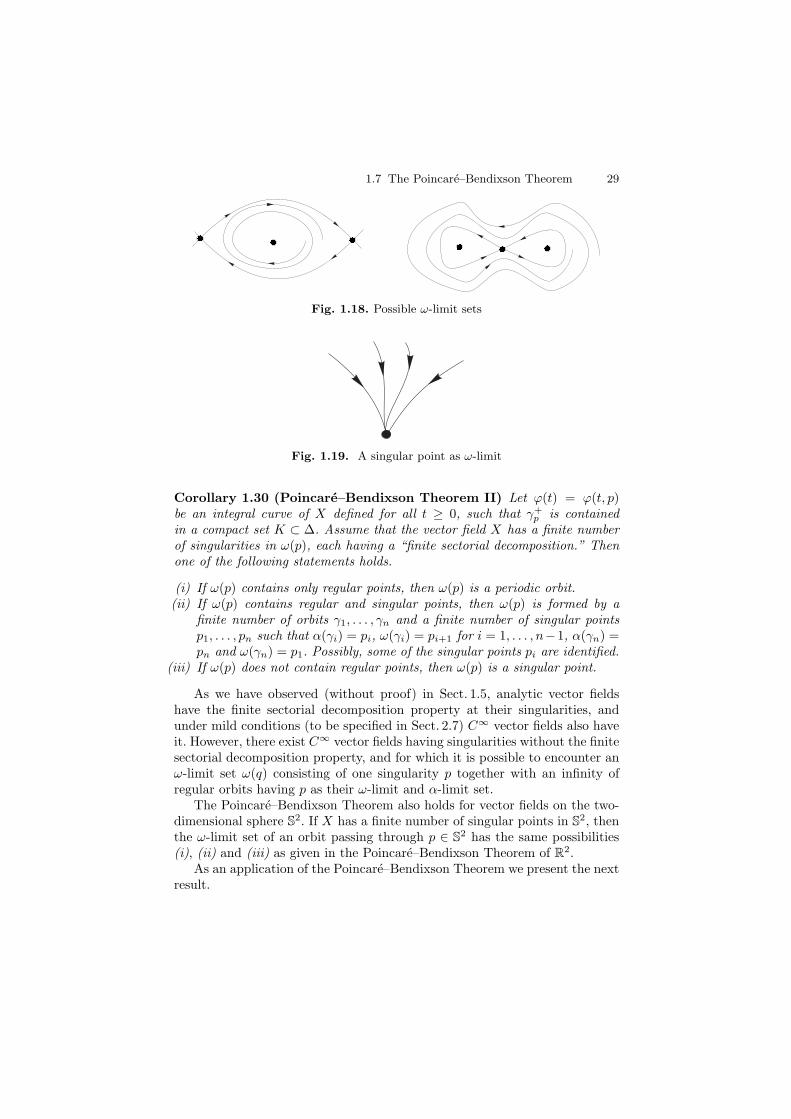
1.7 The Poincare–Bendixson Theorem 29
Fig. 1.18. Possible ω-limit sets
Fig. 1.19. A singular point as ω-limit
Corollary 1.30 (Poincare–Bendixson Theorem II) Let ϕ(t) = ϕ(t, p)be an integral curve of X defined for all t ≥ 0, such that γ+
p is containedin a compact set K ⊂ Δ. Assume that the vector field X has a finite numberof singularities in ω(p), each having a “finite sectorial decomposition.” Thenone of the following statements holds.
(i) If ω(p) contains only regular points, then ω(p) is a periodic orbit.(ii) If ω(p) contains regular and singular points, then ω(p) is formed by a
finite number of orbits γ1, . . . , γn and a finite number of singular pointsp1, . . . , pn such that α(γi) = pi, ω(γi) = pi+1 for i = 1, . . . , n−1, α(γn) =pn and ω(γn) = p1. Possibly, some of the singular points pi are identified.
(iii) If ω(p) does not contain regular points, then ω(p) is a singular point.
As we have observed (without proof) in Sect. 1.5, analytic vector fieldshave the finite sectorial decomposition property at their singularities, andunder mild conditions (to be specified in Sect. 2.7) C∞ vector fields also haveit. However, there exist C∞ vector fields having singularities without the finitesectorial decomposition property, and for which it is possible to encounter anω-limit set ω(q) consisting of one singularity p together with an infinity ofregular orbits having p as their ω-limit and α-limit set.
The Poincare–Bendixson Theorem also holds for vector fields on the two-dimensional sphere S2. If X has a finite number of singular points in S2, thenthe ω-limit set of an orbit passing through p ∈ S2 has the same possibilities(i), (ii) and (iii) as given in the Poincare–Bendixson Theorem of R2.
As an application of the Poincare–Bendixson Theorem we present the nextresult.

30 1 Basic Results on the Qualitative Theory of Differential Equations
Theorem 1.31 Let X be a vector field of class C1 on an open set Δ ⊂ R2.If γ is a periodic orbit of X such that Int(γ) ⊂ Δ, then there exists a singularpoint of X contained in Int(γ).
Proof. We will suppose that there are no singular points in Int(γ). We considerthe set Γ of closed orbits of X contained in Int(γ), ordered with the followingpartial order: γ1 ≤ γ2 if and only if Int(γ1) ⊇ Int(γ2).
We will show that any completely ordered subset S of Γ (i.e., γ1 �= γ2 inS implies that either γ1 < γ2 or γ1 > γ2), admits an upper bound; that is, anelement greater than or equal to any other element of S.
Let σ = ∩{Int(γi) : γi ∈ S}. We see that σ �= ∅, since every Int(γi) iscompact and the family {Int(γi) : γi ∈ S} has the finite intersection property.That is, any finite intersection of elements of a family cannot be empty. Letq ∈ σ. From the Poincare–Bendixson Theorem, ω(q) is a closed orbit containedin σ, since this set is invariant under X and does not contain singular points.This orbit is an upper bound of S.
From Zorn’s Lemma, Γ has a maximal element. So there does not existany element of Γ contained in Int(μ). But if p ∈ Int(μ), α(p) and ω(p) areclosed orbits by the Poincare–Bendixson Theorem (since there do not existsingular points). As α(p) and ω(p) cannot be both equal to μ, one of them willbe contained in Int(μ). This contradiction proves that there must be singularpoints in Int(μ). ⊓⊔
1.8 Lyapunov Functions
In trying to follow orbits in order to detect their asymptotic behavior, it isoften interesting to use the method of Lyapunov functions.
Therefore, throughout this section, we will consider a C1 vector field X :Δ ⊂ R2 → R2 defined on some open set Δ ⊂ R2 (it in fact suffices to requirethat X be locally Lipschitz) and we denote by φ(p, t) its flow, defined on someopen domain D ⊂ R2 × R. Let f : Δ ⊂ R2 → R be a C1 function; then forp ∈ Δ, the derivative of the function f along the solution φ(p, t) is given by
Xf(p) = ddtf(φ(p, t)) = Dfp(X(p)) =< ∇fp, X(p) >
= ∂f∂x (p)X1(p) + ∂f
∂y (p)X2(p),(1.4)
where ∇fp = ∇f(p) denotes the gradient of f at p. It is common to also
denote Xf(p) by f(p).
Definition 1.32 Under the condition expressed earlier, f is called a Lya-punov function for X if f(p) = Xf(p) < 0 on Δ.
By definition a Lyapunov function is strictly decreasing along the orbitsof f , meaning, among other things, that X is everywhere transverse to the
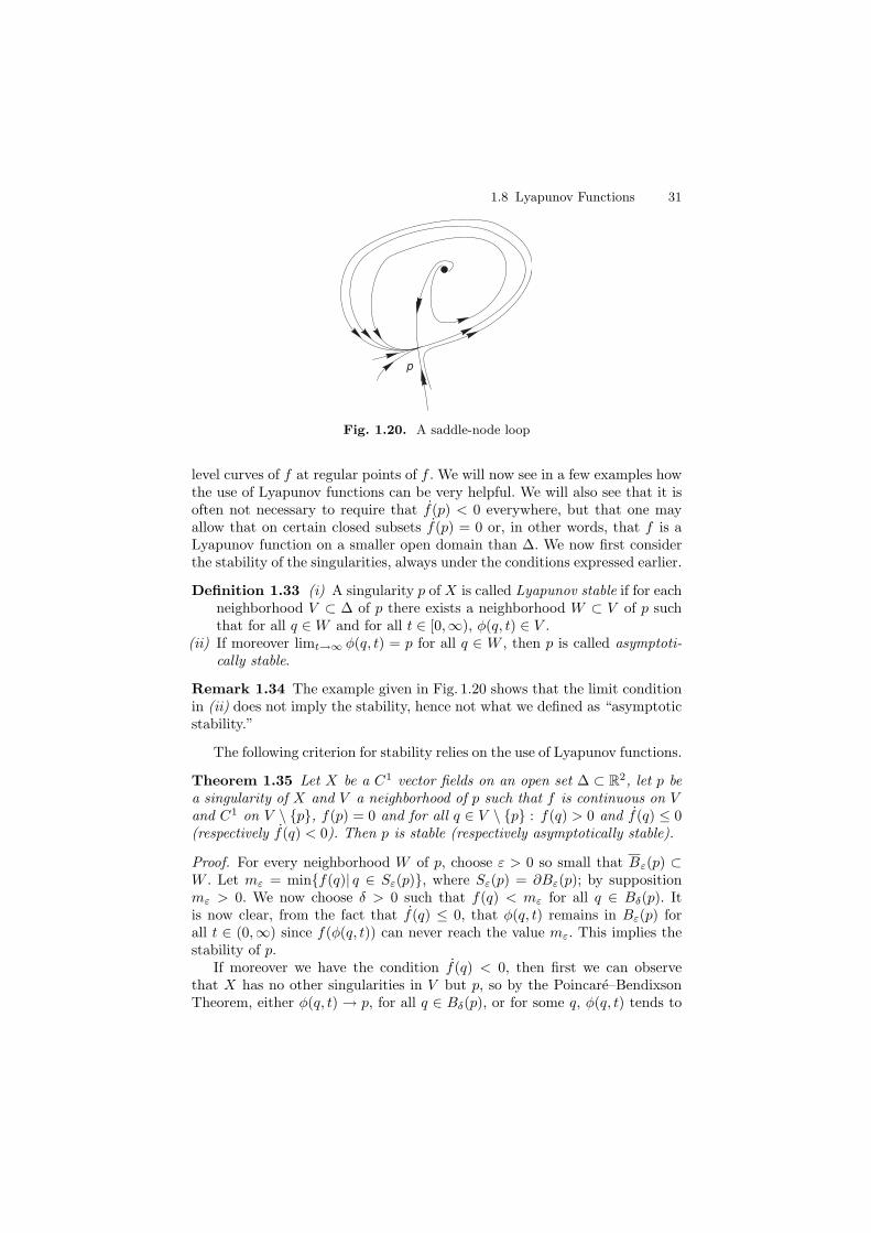
1.8 Lyapunov Functions 31
p
Fig. 1.20. A saddle-node loop
level curves of f at regular points of f . We will now see in a few examples howthe use of Lyapunov functions can be very helpful. We will also see that it isoften not necessary to require that f(p) < 0 everywhere, but that one mayallow that on certain closed subsets f(p) = 0 or, in other words, that f is aLyapunov function on a smaller open domain than Δ. We now first considerthe stability of the singularities, always under the conditions expressed earlier.
Definition 1.33 (i) A singularity p of X is called Lyapunov stable if for eachneighborhood V ⊂ Δ of p there exists a neighborhood W ⊂ V of p suchthat for all q ∈ W and for all t ∈ [0,∞), φ(q, t) ∈ V .
(ii) If moreover limt→∞ φ(q, t) = p for all q ∈ W , then p is called asymptoti-cally stable.
Remark 1.34 The example given in Fig. 1.20 shows that the limit conditionin (ii) does not imply the stability, hence not what we defined as “asymptoticstability.”
The following criterion for stability relies on the use of Lyapunov functions.
Theorem 1.35 Let X be a C1 vector fields on an open set Δ ⊂ R2, let p bea singularity of X and V a neighborhood of p such that f is continuous on Vand C1 on V \ {p}, f(p) = 0 and for all q ∈ V \ {p} : f(q) > 0 and f(q) ≤ 0(respectively f(q) < 0). Then p is stable (respectively asymptotically stable).
Proof. For every neighborhood W of p, choose ε > 0 so small that Bε(p) ⊂W . Let mε = min{f(q)| q ∈ Sε(p)}, where Sε(p) = ∂Bε(p); by suppositionmε > 0. We now choose δ > 0 such that f(q) < mε for all q ∈ Bδ(p). Itis now clear, from the fact that f(q) ≤ 0, that φ(q, t) remains in Bε(p) forall t ∈ (0,∞) since f(φ(q, t)) can never reach the value mε. This implies thestability of p.
If moreover we have the condition f(q) < 0, then first we can observethat X has no other singularities in V but p, so by the Poincare–BendixsonTheorem, either φ(q, t) → p, for all q ∈ Bδ(p), or for some q, φ(q, t) tends to
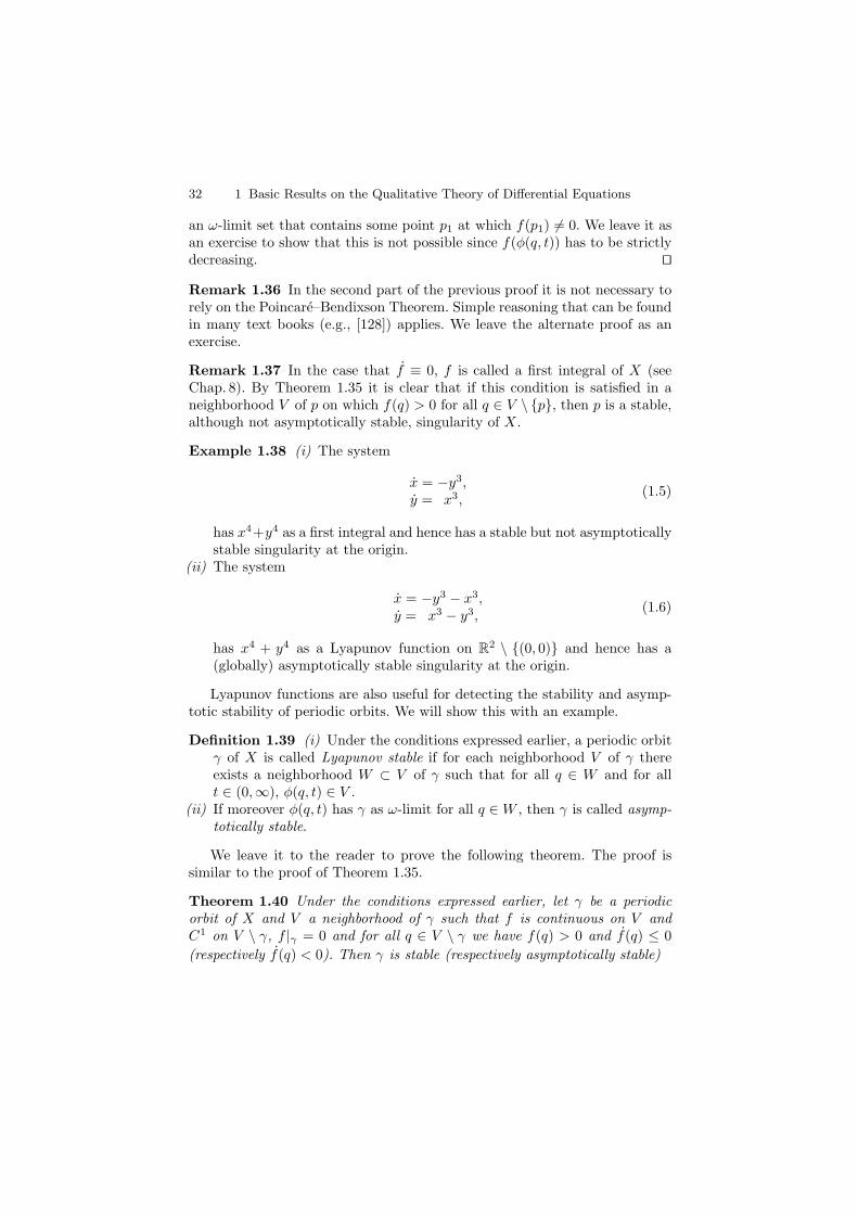
32 1 Basic Results on the Qualitative Theory of Differential Equations
an ω-limit set that contains some point p1 at which f(p1) �= 0. We leave it asan exercise to show that this is not possible since f(φ(q, t)) has to be strictlydecreasing. ⊓⊔
Remark 1.36 In the second part of the previous proof it is not necessary torely on the Poincare–Bendixson Theorem. Simple reasoning that can be foundin many text books (e.g., [128]) applies. We leave the alternate proof as anexercise.
Remark 1.37 In the case that f ≡ 0, f is called a first integral of X (seeChap. 8). By Theorem 1.35 it is clear that if this condition is satisfied in aneighborhood V of p on which f(q) > 0 for all q ∈ V \ {p}, then p is a stable,although not asymptotically stable, singularity of X.
Example 1.38 (i) The system
x = −y3,y = x3,
(1.5)
has x4+y4 as a first integral and hence has a stable but not asymptoticallystable singularity at the origin.
(ii) The system
x = −y3 − x3,y = x3 − y3,
(1.6)
has x4 + y4 as a Lyapunov function on R2 \ {(0, 0)} and hence has a(globally) asymptotically stable singularity at the origin.
Lyapunov functions are also useful for detecting the stability and asymp-totic stability of periodic orbits. We will show this with an example.
Definition 1.39 (i) Under the conditions expressed earlier, a periodic orbitγ of X is called Lyapunov stable if for each neighborhood V of γ thereexists a neighborhood W ⊂ V of γ such that for all q ∈ W and for allt ∈ (0,∞), φ(q, t) ∈ V .
(ii) If moreover φ(q, t) has γ as ω-limit for all q ∈ W , then γ is called asymp-totically stable.
We leave it to the reader to prove the following theorem. The proof issimilar to the proof of Theorem 1.35.
Theorem 1.40 Under the conditions expressed earlier, let γ be a periodicorbit of X and V a neighborhood of γ such that f is continuous on V andC1 on V \ γ, f |γ = 0 and for all q ∈ V \ γ we have f(q) > 0 and f(q) ≤ 0
(respectively f(q) < 0). Then γ is stable (respectively asymptotically stable)
1.9 Essential Ingredients of Phase Portraits 33
Example 1.41 Consider the system
x = y + (1 − x2 − y2)x,y = −x + (1 − x2 − y2)y.
(1.7)
We see that γ = S1 = {(x, y)|x2 + y2 = 1} is a periodic orbit, while fdefined by
f(x, y) =
{1 − (x2 + y2) when x2 + y2 < 1
(x2 + y2) − 1 when x2 + y2 > 1,
satisfies the conditions of Theorem 1.40 on R2 \ {(0, 0)}. As such, γ is stableand moreover all orbits in R2 \ {(0, 0)} have γ as their ω-limit set.
1.9 Essential Ingredients of Phase Portraits
For linear vector fields it is possible to describe all conjugacy classes, but thisis not possible when we study non-linear vector fields. However, there existsa general characterization of the topological equivalence classes for vectorfields on the plane. To present it we will introduce some definitions. Thesedefinitions together with Proposition 1.42 and Theorem 1.43 can be foundin [107] and [116]. In these works much more general situations are considered.
In this section we do not need X to be C1; it need only be sufficientlyregular to admit the existence of a continuous flow (local Lipchitz continuitysuffices). We consider a differential equation x = X(x) where X is a locallyLipschitz function on R2 and let φ(s, x) be the flow defined by the differentialequation. Following the notation of the works of Markus and Neumann, wedenote by (R2, φ) the flow defined by the differential equation. By the theoremof continuous dependence on initial conditions, the flow (R2, φ) is continuous.
We say that a flow (R2, φ) is a parallel flow if it is topologically equivalentto one of the following flows:
(i) The flow defined on R2 by the differential system x = 1, y = 0, which wedenote by strip flow.
(ii) The flow defined on R2 \ {0} by the differential system given in polarcoordinates r′ = 0, θ′ = 1, which we denote by annulus flow.
(iii) The flow defined on R2 \ {0} by the differential system given in polarcoordinates r′ = r, θ′ = 0, which we denote by spiral or nodal flow.
Given a maximal open region on R2 on which the flow is parallel, it isinteresting to know the orbit-structure of its boundary. Clearly following typesof orbits can be present:
(i) a singular point,
34 1 Basic Results on the Qualitative Theory of Differential Equations
(ii) a periodic orbit for which there does not exist a neighborhood entirelyconsisting of periodic orbits,
(iii) an orbit γ(p), homeomorphic to R for which there does not exist a neigh-borhood N of γ(p) such that(1) For all q ∈ N α(q) = α(p) and ω(q) = ω(p),(2) The boundary ∂N of N , that is ∂N = N \N , is formed by α(p), ω(p)
and two orbits γ(q1) and γ(q2) such that α(p) = α(q1) = α(q2) andω(p) = ω(q1) = ω(q2).
Orbits satisfying (i), (ii) or (iii) are called “separatrices” in [107] and [116].In this book we prefer to keep the name separatrix for an orbit satisfying(iii), meaning for instance that a linear saddle has four separatrices. Indeed,orbits limiting on a singularity and bordering a hyperbolic sector are alwaysseparatrices. We also remark that for analytic flows, the orbits satisfying (ii)are the limit cycles. In view of presenting the next result we introduce theseparatrix skeleton consisting of the set of all orbits satisfying either (i) or(iii); if we also add the orbits satisfying (ii) we speak about the extendedseparatrix skeleton. It is easy to see that the union S of all orbits in theextended separatrix skeleton is a closed set invariant under the flow. Let V bea (maximal) connected component of R2 \ S. It necessarily is invariant underthe flow. We call V a canonical region.
Proposition 1.42 Every canonical region of (R2, φ) is parallel, given by ei-ther a strip, an annular or a spiral flow.
Proof. Let U be a canonical region of the C0 flow (R2, φ). We denote the flowφ on U by (U, φ′) with φ′ = φ|U where U does not contain singularities. Sincethere are no separatrices in U nor closed orbits satisfying (ii), the set consistingof orbits homeomorphic to S1 is open, and similarly the set consisting of orbitshomeomorphic to R (which we term line orbits) is open. Hence U consistsentirely of closed orbits or entirely of line orbits.
We claim that two orbits of φ′ can be separated by disjoint parallel neigh-borhoods. To prove this, we suppose to the contrary that γ(p) and γ(q) aredistinct orbits (closed or not) which cannot be separated. Then for any parallelneighborhood Np of p, we have q ∈ cl(Np); i.e.,
q ∈⋂
Np
cl(Np) = α(p) ∪ γ(p) ∪ ω(p).
This means that q ∈ α(p) (or q ∈ ω(p)). But this is impossible becauseq ∈ Nq ⊂ U and α(p) ∪ ω(p) ⊂ cl(Nq) \ Nq �⊂ U .
It follows that the quotient space U/φ′, obtained by collapsing orbits of(U, φ′) to points, is a (Hausdorff) connected one dimensional manifold. Hencethe natural projection π : U → U/φ′ is a locally trivial fibering of which thereare only three possibilities, namely the three classes of parallel flows describedearlier. This proves the proposition. ⊓⊔

1.10 Exercises 35
Given a flow (R2, φ) by the completed separatrix skeleton we mean theunion of the extended separatrix skeleton of the flow together with one orbitfrom each one of the canonical regions (it is also called separatrix configura-tion by other authors). Let C1 and C2 be the completed separatrix skeletonsof the flows (R2, φ1) and (R2, φ2), respectively. We say that C1 and C2 aretopologically equivalent if there exists a homeomorphism from R2 to R2 thatmaps the orbits of C1 to the orbits of C2 preserving the orientation.
Theorem 1.43 (Markus–Neumann–Peixoto Theorem) Assume that(R2, φ1) and (R2, φ2) are two continuous flows with only isolated singularpoints. Then these flows are topologically equivalent if and only if their com-pleted separatrix skeletons are equivalent.
From this result, it is enough to describe the completed separatrix skeletonin order to determine the topological equivalence class of a differential system.
1.10 Exercises
Exercise 1.1 Let X be a linear vector field on a neighborhood of 0 ∈ R2, withX(0) = 0, and denote by ϕ(t, x) the flow of X. Show that Dxϕ(t, 0) = eAt,with A = DX(0).
Exercise 1.2 Consider the equation x′′ = F (x) defined on an interval of R,which corresponds to an one dimensional conservative system. Clearly this isequivalent to the system
x = v,
v = F (x).(1.8)
(i) Prove that the total energy E = T + U is a first integral of (1.8) whereT (v) = v2/2 is the kinetic energy and U(x) = −
∫ x
x0F (z)dz is the potential
energy.(ii) Prove that all the singular points of (1.8) are on the x-axis. Prove also
that all the periodic orbits of (1.8) intersect the x-axis and are symmetricwith respect to it.
(iii) Prove that if U(x1) = U(x2) = c, U ′(xj) �= 0 for j = 1, 2 and U(x) < cfor all x1 < x < x2, then (1.8) has a periodic orbit passing through thepoints (x1, 0) and (x2, 0).Hint: An orbit that passes through (x0, 0) is given by v2/2 + V (x) = Ewhere E is its energy. Use the fact that dv/dx = F (x)/v to conclude thatthis orbit must again cut the x-axis and that this must happen at (x2, 0).Then use (ii).
(iv) Assume that F (x) �= 0 for 0 < |x− x0| < a. Prove that (1.8) has a centeror a saddle at (x0, 0) when U(x0) is a relative minimum or maximum.
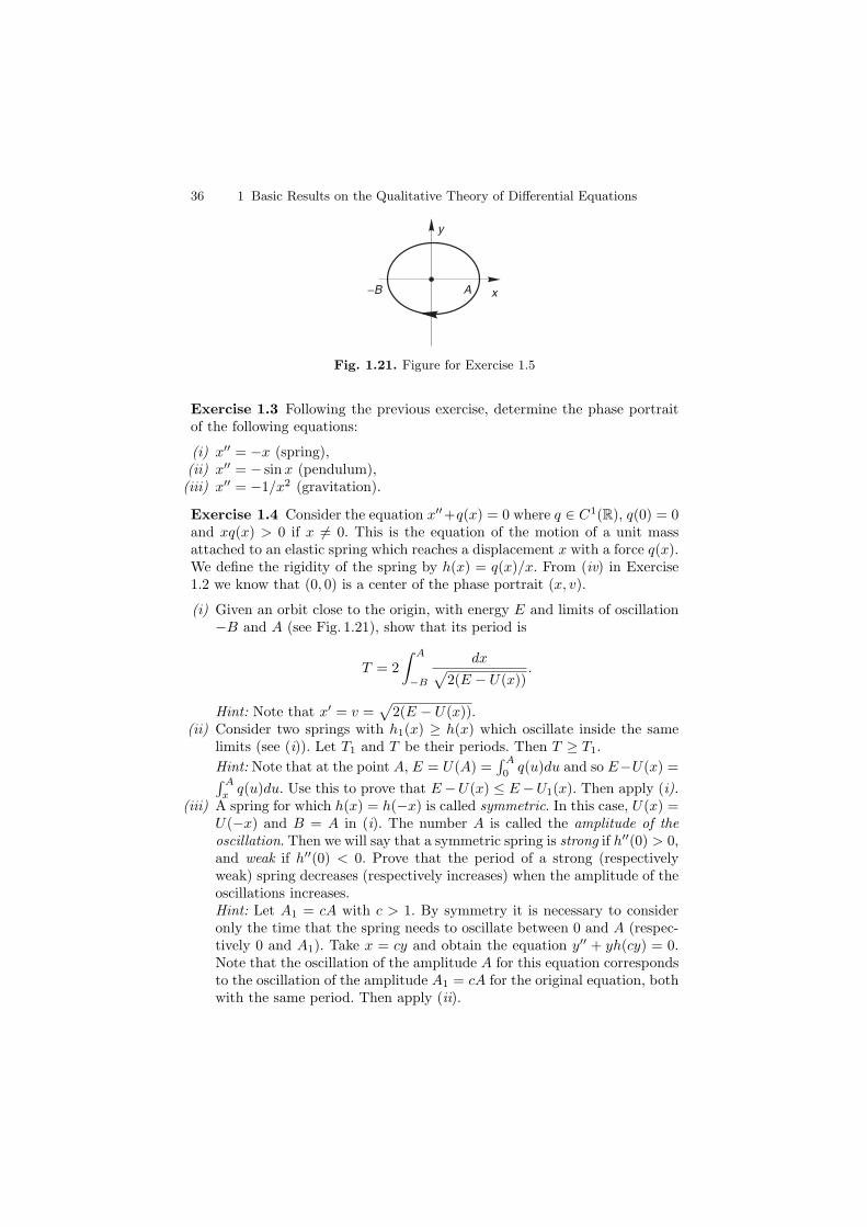
36 1 Basic Results on the Qualitative Theory of Differential Equations
−B A x
y
Fig. 1.21. Figure for Exercise 1.5
Exercise 1.3 Following the previous exercise, determine the phase portraitof the following equations:
(i) x′′ = −x (spring),(ii) x′′ = − sin x (pendulum),(iii) x′′ = −1/x2 (gravitation).
Exercise 1.4 Consider the equation x′′+q(x) = 0 where q ∈ C1(R), q(0) = 0and xq(x) > 0 if x �= 0. This is the equation of the motion of a unit massattached to an elastic spring which reaches a displacement x with a force q(x).We define the rigidity of the spring by h(x) = q(x)/x. From (iv) in Exercise1.2 we know that (0, 0) is a center of the phase portrait (x, v).
(i) Given an orbit close to the origin, with energy E and limits of oscillation−B and A (see Fig. 1.21), show that its period is
T = 2
∫ A
−B
dx√2(E − U(x))
.
Hint: Note that x′ = v =√
2(E − U(x)).(ii) Consider two springs with h1(x) ≥ h(x) which oscillate inside the same
limits (see (i)). Let T1 and T be their periods. Then T ≥ T1.
Hint: Note that at the point A, E = U(A) =∫ A
0q(u)du and so E−U(x) =∫ A
xq(u)du. Use this to prove that E −U(x) ≤ E −U1(x). Then apply (i).
(iii) A spring for which h(x) = h(−x) is called symmetric. In this case, U(x) =U(−x) and B = A in (i). The number A is called the amplitude of theoscillation. Then we will say that a symmetric spring is strong if h′′(0) > 0,and weak if h′′(0) < 0. Prove that the period of a strong (respectivelyweak) spring decreases (respectively increases) when the amplitude of theoscillations increases.Hint: Let A1 = cA with c > 1. By symmetry it is necessary to consideronly the time that the spring needs to oscillate between 0 and A (respec-tively 0 and A1). Take x = cy and obtain the equation y′′ + yh(cy) = 0.Note that the oscillation of the amplitude A for this equation correspondsto the oscillation of the amplitude A1 = cA for the original equation, bothwith the same period. Then apply (ii).
1.10 Exercises 37
Exercise 1.5 Let a, b, c, d be real numbers and f, g : B → R functions ofclass C1 defined in a ball B with center at the origin (0, 0) of R2 and radiusr. The system
x = ax + by + f(x, y),
y = cx + dy + g(x, y),(1.9)
is called a perturbed system of the linear system
x = ax + by,
y = cx + dy.
(i) Prove that if f = O(r), g = O(r) and ad − bc �= 0, then the origin (0, 0)is an isolated singular point of (1.9). As usual, f = O(r) means thatf = rF (x, y) with F (x, y) bounded in a neighborhood of the origin.
(ii) Suppose that f = g = 0. Determine the conditions on a, b, c, d such that(0, 0) is a hyperbolic singularity of (1.9). In this case, describe the phaseportrait of (1.9) in a neighborhood of the origin. There are three topolog-ical types.
(iii) Describe the phase portraits of the systems later. Show that they are nottopologically equivalent each other or to the types found in (ii).
x = x2, y = −y,
x = e−1/x2
sin1
x, y = −y.
Exercise 1.6 Let X be a C1 vector field on Δ ⊂ R2. Prove that if ϕ(t) isa trajectory of X defined on the maximal interval (ω−, ω+) and such thatlimt→ω+
ϕ(t) = p ∈ Δ, then ω+ = ∞ and p is a singular point of X.
Exercise 1.7 Let ϕ(t, x) be the flow generated by a C1 vector field X on R2.A non-empty subset S ⊂ R2 is called minimal (for X) if it is invariant (i.e.,if x ∈ S then ϕ(t, x) ∈ S for all t ∈ R), compact, and does not contain propersubsets with these properties.
Prove that in R2, the only minimal subsets for X are the singular pointsand the periodic orbits of X.
Exercise 1.8 Determine ω(p) and α(p) for p ∈ R2 and for the vector fieldZ = (X,Y ) given by
X = − y + x(x2 + y2) sin
(π√
x2 + y2
),
Y =x + y(x2 + y2) sin
(π√
x2 + y2
).
Hint: Study the inner product 〈(x, y), Z(x, y)〉 = xX + yY .
38 1 Basic Results on the Qualitative Theory of Differential Equations
Exercise 1.9 Determine the set ω(p) for all p ∈ R2 for the system
x = y[y2 + (x2 − 1)2] + x(1 − x2 − y2),
y = − y[y2 + (x2 − 1)2] + y(1 − x2 − y2).
Hint: The same as in the previous exercise.
Exercise 1.10 Determine the singular points of the system
x = y,
y = − b sin x − ay,
with a, b > 0. Assuming that it has no periodic orbits, make a sketch of thephase portrait for this system.
Exercise 1.11 Prove that
x = 2x − x5 − xy4,
y = y − y3 − x2y,
has no periodic orbits.Hint: Show that all singularities of this system are on the coordinate axes.
Consider the phase portrait of this system restricted to the axes and provethat the existence of a closed orbit provides a contradiction.
Exercise 1.12 Let X be a C1 vector field on R2. Let p be a regular point ofX such that p ∈ ω(p). Then ω(p) is a periodic orbit.
Exercise 1.13 Let X be a C1 vector field on R2 and γ an orbit of X. Provethat if γ is not a periodic orbit, then either it is a singular point or ω(γ) ∩α(γ) = ∅.
Exercise 1.14 Let X be a C1 vector field on R2 such that there exists aneighborhood V of the origin on which X|V is the linear vector field
(x1, x2) → (λ1x1, λ2x2)
with λ1λ2 < 0 and λ1 + λ2 < 0.Let L = γp∪{(0, 0)} be like in Fig. 1.22, and JL be the bounded connected
component of R2 \ L. Prove that there exists a neighborhood WL of L suchthat for all q ∈ WL ∩ JL we have that ω(q) = L.
Hint: Consider Fig. 1.22. Note that it is possible to define a Poincare mapπ for the loop L using the transverse segment Σ which is contained in theupper side of the square. Prove that π = f ◦ g where g maps points from thissegment to Σ0 and f : Σ0 → Σ. Prove that g(x) = xθ with θ > 1 and concludethat π′(x) < 1.

1.10 Exercises 39
0 S0
S
g
f
JL
p
gp
Fig. 1.22. Hint for Exercise 1.14
Exercise 1.15 Prove that the origin is an asymptotically stable singularpoint of the system
x = − x − x3
3− 2 sin y,
y = − y − y3
3.
That is, prove that the ω-limit of every solution in a neighborhood of theorigin is the origin.
Exercise 1.16 Let f : R2 → R2 be a C1 function such that f(0, 0) = (0, 0)and 〈x, f(x)〉 < 0 for all x �= 0. Prove that x → |x|2 is a Lyapunov functionfor the system x′ = f(x).
Exercise 1.17 Let X be a C1 vector field on some open domain Δ ⊂ R2. LetS = {p ∈ Δ : X(p) = 0} and let f : Δ \ S → R be a C1 Lyapunov functionfor X on Δ \ S. Show that for all q ∈ Δ \ S, ω(q) ⊂ S.
Exercise 1.18 Let Δ ⊂ R2 be an open set and V : Δ → R a C2 function.The gradient vector field associated to V is defined by x = −gradV (x) forx ∈ Δ where
gradV (x) =
(∂V
∂x1(x),
∂V
∂x2(x)
).
40 1 Basic Results on the Qualitative Theory of Differential Equations
Note that the C1 vector field gradV satisfies
DVx · y =< gradV (x), y >,
for all x ∈ Δ and y ∈ R2. Let V be a derivative of V along the trajectories ofthe field. Prove:
(i) V (x) ≤ 0 for all x ∈ Δ, and V (x) = 0 if and only if x is a singularity ofgradV .
(ii) If x0 is an isolated minimum of V , then x0 is an asymptotically stablesingularity of −gradV .
(iii) −gradV does not have periodic solutions.
Exercise 1.19 Let X = ∇f = gradf , where f is a Cr function, r ≥ 2,defined on an open set Δ ⊂ R2. Prove that X has no periodic orbits. If X hasonly isolated singular points, then for all p ∈ Δ the ω-limit set of p is eitherempty or is a singular point.
Hint: If ϕ(t) is a trajectory of X note that df(ϕ(t))/dt > 0; that is, f ◦ ϕis an increasing function.
Exercise 1.20 Let Δ ⊂ R2 be open and let V : Δ → R be of class C2. Givenc ∈ R, the set V −1(c) is called a level of V . If x ∈ V −1(c) is a regular point(that is, DVx �= 0), then V −1(c) is a C1 curve near x. Prove that in this case,gradV (x) is perpendicular to V −1(c) at x. For each case later, make a sketchof the graph of V and of the phase portrait of −gradV .
(i) V (x, y) = x2 + y2;(ii) V (x, y) = x2 − y2;(iii) V (x, y) = x4 − x2 + y2.
Exercise 1.21 Let f : R2 → R2 be a C1 function such that f(0, 0) = (0, 0).The singular point (0, 0) ∈ R2 is called globally stable when is stable andlimt→∞ ϕ(t) = (0, 0) for every solution ϕ(t) of
x′ = f(x). (1.10)
Let V : R2\{(0, 0)} → R be a Lyapunov function of system (1.10). Supposethat for every c > 0 there exists R > 0 such that if |x| > R then V (x) > c forall x ∈ R2. Then (0, 0) is a globally stable solution of (1.10). Note that thecondition {x ∈ R2 : V (x) = 0} = {(0, 0)} is not necessary. It is sufficient tosuppose that this set does not contain a full trajectory different from x(t) =(0, 0).
Exercise 1.22 Let f : R → R be a C1 function such that f(0) = 0. Considerthe system
x′′ + ax′ + f(x) = 0, (1.11)
for x ∈ R. If a > 0 and f(x)x > 0 for all x �= 0, then a null solution is anasymptotically stable solution for system (1.11) (that is, the corresponding
1.11 Bibliographical Comments 41
solution for the associated first order system on R2 is an asymptotically stablesolution). If f(x)/x > ε > 0 for all x �= 0, then a null solution is globally stable(see Exercise 1.21).
Hint: Take V (x, y) = y2 + 2
∫ x
0
f(x)dx.
Exercise 1.23 Under the assumptions that a < 0 < b, F, g ∈ C1(a, b),xg(x) > 0 for x �= 0, G(x) =
∫ x
0g(s)ds → ∞ as x → a if a = −∞
and G(x) → ∞ as x → b if b = ∞, f(x)/g(x) is monotone increasing on(a, 0)∪ (0, b) and is not constant on any neighborhood of x = 0, it follows thatthe system
x = y − F (x),
y = − g(x),
has at most one limit cycle in the region a < x < b and if exists it is stable.
Exercise 1.24 Under the assumptions that g(x) = x, F ∈ C1(R), f(x) =F ′(x) is an even function with exactly two positive zeros a1 < a2 with F (a1) >0 and F (a2) < 0, and f(x) is monotone increasing for x > a2, it follows thatthe system from previous exercise has at most two limit cycles.
1.11 Bibliographical Comments
For a deeper introduction to the topics of this chapter, the reader can lookat the following books: Chow and Hale [35], Guckenheimer and Holmes [77],Hirsch and Smale [84], Hartman [80], Sotomayor [151], Zhang, Ding, Huangand Dong [169] and mainly the book of Sotomayor [152]. Many of the proofsof the results of this chapter are translations of the corresponding proofs fromthe book of Sotomayor [152].
The results related to Theorem 1.20 are due to several authors. Condition(i) was obtained by Bendixson [15]; and (ii) and (iii) were proved by Berlinskii[16] and [17]. For results on the number of parabolic sectors p we refer toSagalovich [138] and [139].
The proof of Theorem 1.43 is due to Markus [108], to Neumann [116] andto Peixoto [123].

2
Normal Forms and Elementary Singularities
In this chapter we study the elementary singular points; i.e., the hyperbolicand semi-hyperbolic singular points. The first are those singular points havingtwo eigenvalues with non-zero real part, the second have a unique non-zeroeigenvalue. We also provide complete information about invariant manifoldsas well as good normal forms for such singularities.
2.1 Formal Normal Form Theorem
Since it is no simpler to limit to R2, we present the general normal formtheorem for C∞ vector fields on Rn.
Let X = A+f be a vector field on Rn with A linear, and f a C∞ functionsuch that f(0) = 0 and Df(0) = 0. The aim of a normal form theory isto determine for each given linear vector field A a restricted class of non-linearities Fn as small and as simple as possible, and such that for each f ,the equation can, by appropriate C∞ coordinate change, be brought to theform X ′ = A + f with f ∈ Fn. We also recall that a Cr coordinate changeh, with r ≥ 1, operates on a vector field X1 to change it into X2 as given byexpression (1.2), namely
Dhh−1(p)X1(h−1(p)) = X2(p);
we also write X2 = h∗X1.In view of finding appropriate coordinate changes, consider for each m ∈ N
with m ≥ 1 the so called “adjoint action”:
admA : Hm(Rn) →Hm(Rn)
X → [A,X],
where Hm(Rn) denotes the set of polynomial vector fields on Rn which arehomogeneous of degree m. Here, [A,X] = A ◦ X − X ◦ A, seen as differentialoperators. Let Bm = admA(Hm(Rn)) and let Gm be any complement of Bm,i.e., Bm ⊕ Gm = Hm(Rn).
44 2 Normal Forms and Elementary Singularities
Theorem 2.1 (Formal Normal Form Theorem) Let X be a Cr vectorfield defined in a neighborhood of 0 with X(0) = 0 and DX(0) = A, r ∈ N
with r ≥ 1. Let Bk and Gk be as above. Then there is an analytic change ofcoordinates φ : (Rn, 0) → (Rn, 0) in a neighborhood of 0 such that X ′ = φ∗(X)is of the form
X ′(y) = Ay + g2(y) + · · · + gr(y) + o(‖y‖r)
with gi ∈ Gi, for all i = 2, . . . , r.
Proof. The proof proceeds by induction on 2 ≤ s < r. We assume that
X(x) = A(x) + g2(x) + · · · + gs−1(x) + fs(x) + o(‖x‖s),
with gi ∈ Gi, for all i = 2, . . . , s − 1 and fs is homogeneous of degree s. Wetry a coordinate transformation of the form
x = h(y) = y + P (y),
where P is a homogeneous (vector valued) polynomial of degree s, which needsto be determined. Substitution gives
(I + DP (y))y = A(y + P (y)) + g2(y) + · · · + gs−1(y) + fs(y) + o(‖y‖s)
or
y = (I + DP (y))−1[Ay + g2(y) + · · · + gs−1(y) + fs(y) + AP (y) + o(‖y‖s)]
= (I − DP (y) + O(‖y‖s))[Ay + · · · ]=Ay + g2(y) + · · · + gs−1(y) + fs(y) + AP (y) − DP (y)Ay + o(‖y‖s)].
The (s− 1)-jet of X remains unchanged, while for the terms of order s we get
fs(y) − adsA(P )(y).
Clearly a suitable choice of P will make this term lie in Gs. ⊓⊔
Remark 2.2 The proof we use can be found in [77]. It is constructive, andit can be used to implement the calculation in specific examples.
The original proof in [156] is quite similar but uses the time 1-mapping ofthe flow Pt instead of I + P .
Remark 2.3 Using Theorem 2.1 and Borel’s Theorem (see [19] and [115]) onthe representation of ∞-jets, one can show the following.
If X is a C∞ vector field defined in a neighborhood of 0 ∈ Rn, withX(0) = 0, then there is a C∞ coordinate change φ : (Rn, 0) → (Rn, 0) in aneighborhood of 0 such that X ′ = φ∗(X) has an ∞-jet:
2.1 Formal Normal Form Theorem 45
j∞X ′(0) = A +∞∑
i=2
gi,
with gi ∈ Gi, for all i = 2, 3, . . .. Note that this result is purely formal. Itprovides a simple form for the ∞-jet but not for the vector field itself. Lateron we will see essential differences.
We recall that Borel’s Theorem states that for every p ∈ Rn and for every∞-jet (i.e., formal series in n variables), there exists a C∞ function f definedon a neighborhood of p whose ∞-jet j∞f(p) (i.e., its Taylor series at p) isequal to the given ∞-jet.
Remark 2.4 A great deal of information concerning normal forms can befound in [20]. Especially interesting is the treatment of singular vector fieldsbelonging to special Lie subalgebras like, for instance, Hamiltonian vectorfields, volume preserving vector fields or reversible vector fields (L∗X = −X,with L a linear involution). In these cases one can find normal forms belongingto the same Lie subalgebra, and this for a coordinate change lying in the Liesubgroup belonging to the Lie subalgebra. The presentation of the results isdone in the framework of filtered Lie algebras having the Borel property.
Choice of the Gm From a computational point of view, the normal formtheory presented in this way is not yet satisfactory. An improvement was madein [23] and [61]. It concerns the choice of the complementary spaces Gm.
The idea is that one can always use
Gm = Ker(admAT ),
where AT denotes the transpose of A, defined by 〈AT x, y〉 = 〈x,Ay〉, or equiv-alently (AT )ij = Aji. We give a sketch of the proof, referring to [162] for adetailed elaboration. We consider an inner product 〈 , 〉m on Hm(Rn) de-fined as ⟨ ∑
|σ|=m
aσxσ,∑
|σ|=m
bσxσ
⟩
m
=∑
|σ|=m
σ!〈aσ, bσ〉, (2.1)
for all aσ, bσ ∈ Rm with |σ| = m.For this inner product 〈 , 〉m we have
(admAT ) = (admA)T ,
and hence Hm(Rn) = Im(admA) ⊕ Ker(admA)T .We show by an example that Ker(adAT ) can serve as a complement Gm,
but not Ker(adA). For this take
A =
(0 10 0
).
Look at the 2-jet

46 2 Normal Forms and Elementary Singularities
[y
∂
∂x, xiy2−i ∂
∂x
]= ixi−1y3−i ∂
∂x,
[y
∂
∂x, xiy2−i ∂
∂y
]= ixi−1y3−i ∂
∂y− xiy2−i ∂
∂x.
The image contains xy(∂/∂x), y2(∂/∂x), y2(∂/∂y) − xy(∂/∂x), 2xy(∂/∂y) −x2(∂/∂x). It is four dimensional such that Ker(ad2A) is two-dimensional.
As y2(∂/∂x) ∈ Ker(ad2A), we cannot have Im(ad2A) ⊕ Ker(ad2A) =H2(R2).
For ad2AT we have[x
∂
∂y, xiy2−i ∂
∂x
]= (2 − i)xi+1y1−i ∂
∂x− xiy2−i ∂
∂y,
[x
∂
∂y, xiy2−i ∂
∂y
]= (2 − i)xi+1y1−i ∂
∂y,
and Ker(ad2AT ) is spanned by x2(∂/∂y) and x2(∂/∂x) + xy(∂/∂y).
This gives one possible choice of the normal form; in certain proofs it isbetter to take x2(∂/∂y), xy(∂/∂y) as a basis for G2, because then the 2-jettakes the form y(∂/∂x) + (ax2 + bxy)(∂/∂y) which, for instance, correspondsto a second order scalar differential equation. We will come back to thesenilpotent singularities in Sect. 3.4.
We now start a systematic study of the singularities, starting with theelementary ones.
2.2 Attracting (Repelling) Hyperbolic Singularities
Throughout this section we deal with vector fields that are at least C∞, andhave an attracting or repelling hyperbolic singularity. We always position thesingularity of interest at the origin.
The differential equation X near such a singularity can be written as
x = ax + by + P (x, y),
y = cx + dy + Q(x, y),
with P (0, 0) = Q(0, 0) = DP (0, 0) = DQ(0, 0) = 0, and where the matrix of
DX(0) =
(a bc d
)can be written as
(λ1 00 λ2
),
(λ1 10 λ1
), or
(α β−β α
)
with λ1λ2 > 0, α �= 0 and β > 0.We will now show that such a singularity is locally C0-conjugate to its
linear part. It suffices to give the proof for the attracting case, meaning that
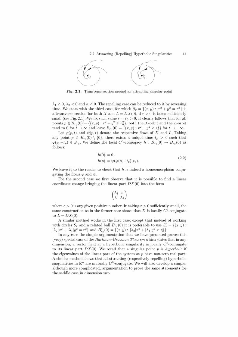
2.2 Attracting (Repelling) Hyperbolic Singularities 47
Fig. 2.1. Transverse section around an attracting singular point
λ1 < 0, λ2 < 0 and α < 0. The repelling case can be reduced to it by reversingtime. We start with the third case, for which Sr = {(x, y) : x2 + y2 = r2} isa transverse section for both X and L = DX(0), if r > 0 is taken sufficientlysmall (see Fig. 2.1). We fix such value r = r0 > 0. It clearly follows that for allpoints p ∈ Br0
(0) = {(x, y) : x2 + y2 ≤ r20}, both the X-orbit and the L-orbit
tend to 0 for t → ∞ and leave Br0(0) = {(x, y) : x2 + y2 < r2
0} for t → −∞.Let ϕ(p, t) and ψ(p, t) denote the respective flows of X and L. Taking
any point p ∈ Br0(0) \ {0}, there exists a unique time tp > 0 such that
ϕ(p,−tp) ∈ Sr0. We define the local C0-conjugacy h : Br0
(0) → Br0(0) as
follows:
h(0) = 0,
h(p) = ψ(ϕ(p,−tp), tp).(2.2)
We leave it to the reader to check that h is indeed a homeomorphism conju-gating the flows ϕ and ψ.
For the second case we first observe that it is possible to find a linearcoordinate change bringing the linear part DX(0) into the form
(λ1 ε0 λ1
)
where ε > 0 is any given positive number. In taking ε > 0 sufficiently small, thesame construction as in the former case shows that X is locally C0-conjugateto L = DX(0).
A similar method works in the first case, except that instead of workingwith circles Sr and a related ball Br0
(0) it is preferable to use S′r = {(x, y) :
|λ2|x2 + |λ1|y2 = r2} and B′r0
(0) = {(x, y) : |λ2|x2 + |λ1|y2 < r20}.
In any case the simple argumentation that we have presented proves this(very) special case of the Hartman–Grobman Theorem which states that in anydimension, a vector field at a hyperbolic singularity is locally C0-conjugateto its linear part DX(0). We recall that a singular point p is hyperbolic ifthe eigenvalues of the linear part of the system at p have non-zero real part.A similar method shows that all attracting (respectively repelling) hyperbolicsingularities in Rn are mutually C0-conjugate. We will also develop a simple,although more complicated, argumentation to prove the same statements forthe saddle case in dimension two.
48 2 Normal Forms and Elementary Singularities
Before proving the Hartman–Grobman Theorem in dimension two, wehowever describe the C∞-conjugacy classes of attracting and repelling hyper-bolic singularities. To that purpose, we start by applying the Formal NormalForm Theorem presented in Sect. 2.1. It depends on the respective JordanNormal Form for the linear part. We restrict to the repelling case.
Case 1: Let DX(0) = λ1x(∂/∂x) + λ2y(∂/∂y) with λ2 ≥ λ1 > 0. The Lie–bracket operation of Sect. 2.1 (dividing all calculations by λ1) gives
[x
∂
∂x+ λy
∂
∂y, xmyn ∂
∂x
]= ((m − 1) + nλ)xmyn ∂
∂x,
[x
∂
∂x+ λy
∂
∂y, xmyn ∂
∂y
]= (m + (n − 1)λ)xmyn ∂
∂y,
with λ = λ2/λ1 ≥ 1. Besides the linear terms we see that all terms in theTaylor development can be removed, except for xm(∂/∂y) in the case λ = m.Based on Borel’s Theorem on the realization of formal power series we henceknow the existence of a C∞ coordinate change near 0 such that the vectorfield can be written as
x = λ1x + f(x, y),
y = λ2y + g(x, y),
where f and g are C∞ functions and j∞f(0, 0) = j∞g(0, 0) = 0, in the caseλ2/λ1 /∈ N.
If λ2 = mλ1 for some m ∈ N with m ≥ 1, then a C∞ normal form is givenby
x = λ1x + f(x, y),
y = λ2y + axm + g(x, y),
for some a ∈ R, where f and g are C∞ functions and j∞f(0, 0) = j∞g(0, 0) =0. By a linear change (x, y) �−→ (bx, δy) for some b ∈ R and δ ∈ {−1, 1} wecan reduce to a = 1.
In Sect. 2.7 we will show that it is possible to reduce to f = g = 0, whichis a special case of Sternberg’s Theorem; see [153]. Before proving this, weconsider the other cases.
Case 2: Let DX(0) = λ(x(∂/∂x) + (x + y)(∂/∂y)) with λ > 0. We againdivide by λ in the Lie-bracket calculations:
[x
∂
∂x+ (x + y)
∂
∂y, xmyn ∂
∂x
]= (m + n − 1)xmyn ∂
∂x+ nxm+1yn−1 ∂
∂x
− xmyn ∂
∂y,
[x
∂
∂x+ (x + y)
∂
∂y, xmyn ∂
∂y
]= (m + n − 1)xmyn ∂
∂y+ nxm+1yn−1 ∂
∂y.
2.3 Hyperbolic Saddles 49
By making the appropriate linear combinations it is clear that all terms oforder at least two can be removed, inducing a C∞ normal form
x = λx + f(x, y),
y = λy + x + g(x, y),
where f and g are C∞ functions and j∞f(0, 0) = j∞g(0, 0) = 0.
Case 3: Let DX(0) = α((x + γy)(∂/∂x) + (−γx + y)(∂/∂y)) with αγ �= 0.We divide by α in the normal form calculations and get
[(x + γy)
∂
∂x+ (−γx + y)
∂
∂y, xmyn ∂
∂x
]= (m + n − 1)xmyn ∂
∂x
+ mγxm−1yn+1 ∂
∂x− nγxm+1yn−1 ∂
∂x+ γxmyn ∂
∂y,
[(x + γy)
∂
∂x+ (−γx + y)
∂
∂y, xmyn ∂
∂y
]= (m + n − 1)xmyn ∂
∂y
+ mγxm−1yn+1 ∂
∂y− nγxm+1yn−1 ∂
∂y− γxmyn ∂
∂x.
Again appropriate linear combinations show that all terms of order at leasttwo can be removed, inducing a C∞ normal form
x = αx + βy + f(x, y),
y = −βx + αy + g(x, y),
where αβ �= 0, f and g are C∞ functions and j∞f(0, 0) = j∞g(0, 0) = 0.In Sect. 2.7 we will show how in all three cases the “flat” terms f and g
can be removed, providing linear normal forms for C∞-conjugacy, except inthe case λ = m ∈ N with m ≥ 1, for which the normal form is
x = λx, y = mλy + δxm, (2.3)
for some λ �= 0 and δ ∈ {0, 1}.In the analytic case it is even possible to prove that the obtained normal
forms can be obtained by an analytic change of coordinates, but we will notprove this. For the proof in the C∞ case we refer to Sect. 2.7.
2.3 Hyperbolic Saddles
2.3.1 Analytic Results
The differential equation X near such a singularity can be written as
x = λ1x + P (x, y),
y = λ2y + Q(x, y),(2.4)
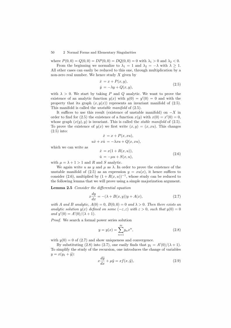
50 2 Normal Forms and Elementary Singularities
where P (0, 0) = Q(0, 0) = DP (0, 0) = DQ(0, 0) = 0 with λ1 > 0 and λ2 < 0.From the beginning we normalize to λ1 = 1 and λ2 = −λ with λ ≥ 1.
All other cases can easily be reduced to this one, through multiplication by anon-zero real number. We hence study X given by
x = x + P (x, y),
y = −λy + Q(x, y),(2.5)
with λ > 0. We start by taking P and Q analytic. We want to prove theexistence of an analytic function y(x) with y(0) = y′(0) = 0 and with theproperty that its graph (x, y(x)) represents an invariant manifold of (2.5).This manifold is called the unstable manifold of (2.5).
It suffices to use this result (existence of unstable manifold) on −X inorder to find for (2.5) the existence of a function x(y) with x(0) = x′(0) = 0,whose graph (x(y), y) is invariant. This is called the stable manifold of (2.5).To prove the existence of y(x) we first write (x, y) = (x, xu). This changes(2.5) into:
x = x + P (x, xu),
ux + xu = −λxu + Q(x, xu),
which we can write asx = x(1 + R(x, u)),
u = −μu + S(x, u),(2.6)
with μ = λ + 1 > 1 and R and S analytic.We again write u as y and μ as λ. In order to prove the existence of the
unstable manifold of (2.5) as an expression y = xu(x), it hence suffices toconsider (2.6), multiplied by (1 + R(x, u))−1, whose study can be reduced tothe following lemma that we will prove using a simple majorization argument.
Lemma 2.5 Consider the differential equation
xdy
dx= −(λ + B(x, y))y + A(x), (2.7)
with A and B analytic, A(0) = 0, B(0, 0) = 0 and λ > 0. Then there exists ananalytic solution y(x) defined on some (−ε, ε) with ε > 0, such that y(0) = 0and y′(0) = A′(0)/(λ + 1).
Proof. We search a formal power series solution
y = y(x) =
∞∑
n=1
ynxn, (2.8)
with y(0) = 0 of (2.7) and show uniqueness and convergence.By substituting (2.8) into (2.7), one easily finds that y1 = A′(0)/(λ + 1).
To simplify the study of the recursion, one introduces the change of variablesy = x(y1 + y):
xdy
dx+ μy = xf(x, y), (2.9)

2.3 Hyperbolic Saddles 51
with f analytic near (0, 0) and with μ = λ + 1 > 1. In the sequel we drop thetildes however and proceed as if (2.9) is the main equation to solve.
It is now easily seen that (2.9) is a recursive relation for the sequence(yn)n after substitution of (2.8). Indeed, when evaluating (2.9) at order xk,one sees in the left-hand side (k+μ)yk, and in the right-hand side one finds anexpression Hk(y1, . . . , yk−1) that involves only lower order coefficients. Thisargument shows the existence of (2.8) solving (2.7) formally, and it also showsthe unicity.
We now take care of the convergence properties. If at any step of the recur-sion we replace the right-hand side by a larger (positive) value, we certainlyget larger values of yk, so one can find bounds for the coefficients by replacingthe right-hand side by an expression that at every step yields a larger value.
Since
f(x, y) =
∞∑
m=0
∞∑
n=0
fmnxmyn
is analytic, we know that |fmn| ≤ Mrmsn for M > 0, r > 0 and s > 0. In thelight of what was said earlier, we consider (2.9), replacing f by
F (x, y) =∞∑
m=0
∞∑
n=0
Mrmsnxmyn =M
(1 − rx)(1 − sy).
The new equation certainly leads to a formal solution that majorizes theoriginal one. We are hence interested in
xdy
dx+ μy =
Mx
(1 − rx)(1 − sy). (2.10)
The recursive relation that is generated by (2.10) can be written down explic-itly, if we multiply both sides of the equation by (1 − sy):
(n + μ)yn − s∑
k+l=n
(k + μ)ykyl = Mrn−1.
Keeping in mind that y0 = 0 this yields
yn =Mrn−1
n + μ+ s
n−1∑
k=1
k + μ
n + μykyn−k.
We again replace this recursion by a “larger” recursion, i.e., a recursion thathas a solution for which all coefficients are larger: we consider
Yn =M
μ + 1rn−1 + s
n−1∑
k=1
YkYn−k.

52 2 Normal Forms and Elementary Singularities
This is the recursion that is generated from the simple equation
Y (x) =M
μ + 1
x
1 − rx+ sY (x)2, Y (0) = 0.
One can easily compute that there is a unique analytic solution Y with radiusof convergence
ρ =μ + 1
r(μ + 1) + 4Ms.
This is a lower bound for the radius of convergence of the solution (2.8) toour original equation (2.7). ⊓⊔
2.3.2 Smooth Results
In the case that we start with an expression (2.5) in which P and Q are onlyC∞, it is possible to prove the existence of a C∞ unstable (respectively stable)manifold. In the same way as in the analytic case, it follows from the nextlemma.
Lemma 2.6 Consider the differential equation
xdy
dx= −(λ + B(x, y))y + A(x), (2.11)
where A and B are C∞ functions, A(0) = 0, B(0, 0) = 0 and λ > 0. Thenthere exists a C∞ solution y(x) defined on some (−ε, ε) with ε > 0, such thaty(0) = 0 and y′(0) = A′(0)/(λ + 1).
Proof. Exactly as in the proof of Lemma 2.5 we can prove the existence of aunique power series
y = g(x) =
∞∑
n=1
ynxn,
with y1 = A′(0)/(λ + 1) such that g(x) is a formal solution of (2.11).Let g(x) be any C∞ function with j∞g(0) = g, of which the existence
is guaranteed by Borel’s Theorem, which permits one to write every formalpower series as the Taylor development of a C∞ function. If we now write
y = Y + g(x),
then (2.11) changes into
xdY
dx= −(λ + B(x, Y ))Y + A(x),
where A and B are C∞ functions, j∞A(0) = 0, B(0, 0) = 0 and λ > 0. Wehence continue working with expression (2.11), having the extra property that
2.3 Hyperbolic Saddles 53
(0,0)
(x0,y 0)
(x0,−y 0)
Fig. 2.2. The flow on the boundary of V0
j∞A(0) = 0. Expression (2.11) can also be represented by the planar system
x = −x,
y = (λ + B(x, y))y − A(x).
We continue working on x ≥ 0, proving the existence of a C∞ solution y(x) on[0, x0] with x0 > 0 and j∞y(0) = 0. Similar reasoning will clearly be possibleon x ≤ 0, too.
On V = [0, x0] × [−y0, y0], for x0 > 0 and y0 > 0 sufficiently small (seeFig. 2.2), we leave it as an exercise to prove that there exists at least one pointon {x0}× [−y0, y0] with the property that the ω-limit of its orbit is (0, 0). Weobserve that because x = −x �= 0 on V , this orbit, completed with the origin,is the graph (x, f(x)) of a continuous function f : [0, x0] → R. In fact f is C∞
for x > 0.We call the graph of f a stable manifold and we now prove that such a
stable manifold is unique.We therefore introduce the new coordinates (x, Y ) = (x, y − f(x)). Since
the coordinate change is C∞ for x > 0, it operates on the vector field X andchanges it into Y given by
x = −x,
Y = Y (λ + F (x, Y + f(x))).(2.12)
At x = 0, this vector field Y extends in a C0 way to Y |{x=0} = X|{x=0}. It isclear that {Y = 0} is the unique stable manifold for Y , implying the unicityof the stable manifold for X, too.
We hence know that an equation like in (2.11) has, for x0 > 0 sufficientlysmall, a unique continuous solution f : [0, x0] → R with f(0) = 0; f is C∞ on(0, x0).
We now prove that f must also be C∞ at 0 and that j∞f(0) = 0. To thatend we take an arbitrary n ∈ N with n ≥ 1 and try a solution of the form
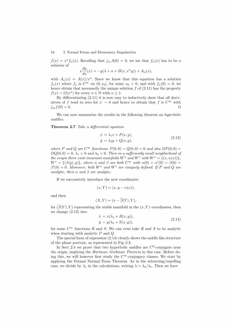
54 2 Normal Forms and Elementary Singularities
f(x) = xnfn(x). Recalling that j∞A(0) = 0, we see that fn(x) has to be asolution of
xdy
dx(x) = −y(λ + n + B(x, xny)) + An(x),
with An(x) = A(x)/xn. Since we know that this equation has a solutionfn(x) where fn is C∞ on (0, x0], for some x0 > 0, and with fn(0) = 0, wehence obtain that necessarily the unique solution f of (2.11) has the propertyf(x) = O(xn) for every n ∈ N with n ≥ 1.
By differentiating (2.11) it is now easy to inductively show that all deriv-atives of f tend to zero for x → 0 and hence to obtain that f is C∞ withj∞f(0) = 0. ⊓⊔
We can now summarize the results in the following theorem on hyperbolicsaddles.
Theorem 2.7 Take a differential equation
x = λ1x + P (x, y),
y = λ2y + Q(x, y),(2.13)
where P and Q are C∞ functions, P (0, 0) = Q(0, 0) = 0 and also DP (0, 0) =DQ(0, 0) = 0, λ1 > 0 and λ2 < 0. Then in a sufficiently small neighborhood ofthe origin there exist invariant manifolds Wu and W s with Wu = {(x, α(x))},W s = {(β(y), y)}, where α and β are both C∞ with α(0) = α′(0) = β(0) =β′(0) = 0. Moreover, both Wu and W s are uniquely defined. If P and Q areanalytic, then α and β are analytic.
If we successively introduce the new coordinates
(x, Y ) = (x, y − α(x)),
and then(X,Y ) = (x − β(Y ), Y ),
for (β(Y ), Y ) representing the stable manifold in the (x, Y )–coordinates, thenwe change (2.13) into
x = x(λ1 + R(x, y)),
y = y(λ2 + S(x, y)),(2.14)
for some C∞ functions R and S. We can even take R and S to be analyticwhen starting with analytic P and Q.
The special form of expression (2.14) clearly shows the saddle like structureof the phase portrait, as represented in Fig. 2.3.
In Sect. 2.4 we prove that two hyperbolic saddles are C0-conjugate nearthe origin, implying the Hartman–Grobman Theorem in this case. Before do-ing this, we will however first study the C∞-conjugacy classes. We start byapplying the Formal Normal Form Theorem. As in the attracting/repellingcase, we divide by λ1 in the calculations, writing λ = λ2/λ1. Then we have
2.4 Topological Study of Hyperbolic Saddles 55
x
y
Fig. 2.3. A hyperbolic saddle
[x
∂
∂x− λy
∂
∂y, xmyn ∂
∂x
]= (m − 1 − nλ)xmyn ∂
∂x,
[x
∂
∂x− λy
∂
∂y, xmyn ∂
∂y
]= (m − (n − 1)λ)xmyn ∂
∂y.
Clearly all terms of order at least two can be removed when λ is irrational. Ifλ = k/l ∈ Q, then the normal form is given by
(1 +
∞∑
i=1
ai(xkyl)i
)x
∂
∂x+
(−k
l+
∞∑
i=1
bi(xkyl)i
)y
∂
∂y.
By using Borel’s Theorem on the realization of formal power series, togetherwith Theorem 2.7, we obtain that a C∞ hyperbolic saddle is C∞-conjugateto one of the following C∞ systems:
x = x(λ1 + R(x, y)),
y = y(λ2 + S(x, y)),(2.15)
with λ2/λ1 ∈ R \ Q and j∞R(0, 0) = j∞S(0, 0) = 0; or
x = x(λ1 + f(xkyl) + R(x, y)),
y = y(λ2 + g(xkyl) + S(x, y)),(2.16)
with λ2/λ1 = k/l ∈ Q and j∞R(0, 0) = j∞S(0, 0) = 0.In Sect. 2.7 we will prove that in both cases the flat terms R and S can be
removed. Unlike the attracting/repelling case the theory of analytic normalforms is not that simple. In starting with an analytic hyperbolic saddle wecannot guarantee the existence of an analytic linearization when λ ∈ R \ Q;neither we can guarantee that f and g are analytic in the case that λ ∈ Q.For more information on this very delicate matter we refer to [148].
2.4 Topological Study of Hyperbolic Saddles
Having the nice C∞ normal forms (for C∞-conjugacy) that one can find, asexplained in Sect. 2.3, it is now easy to prove that two hyperbolic saddles are
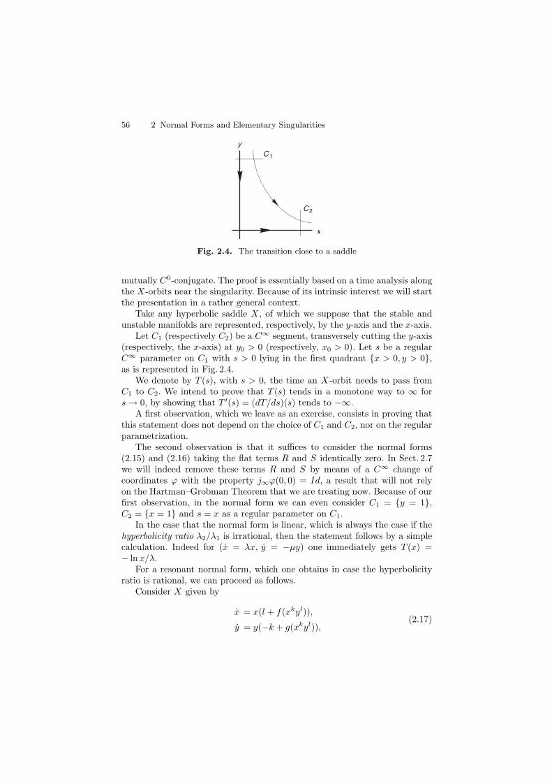
56 2 Normal Forms and Elementary Singularities
x
y
C2
C1
Fig. 2.4. The transition close to a saddle
mutually C0-conjugate. The proof is essentially based on a time analysis alongthe X-orbits near the singularity. Because of its intrinsic interest we will startthe presentation in a rather general context.
Take any hyperbolic saddle X, of which we suppose that the stable andunstable manifolds are represented, respectively, by the y-axis and the x-axis.
Let C1 (respectively C2) be a C∞ segment, transversely cutting the y-axis(respectively, the x-axis) at y0 > 0 (respectively, x0 > 0). Let s be a regularC∞ parameter on C1 with s > 0 lying in the first quadrant {x > 0, y > 0},as is represented in Fig. 2.4.
We denote by T (s), with s > 0, the time an X-orbit needs to pass fromC1 to C2. We intend to prove that T (s) tends in a monotone way to ∞ fors → 0, by showing that T ′(s) = (dT/ds)(s) tends to −∞.
A first observation, which we leave as an exercise, consists in proving thatthis statement does not depend on the choice of C1 and C2, nor on the regularparametrization.
The second observation is that it suffices to consider the normal forms(2.15) and (2.16) taking the flat terms R and S identically zero. In Sect. 2.7we will indeed remove these terms R and S by means of a C∞ change ofcoordinates ϕ with the property j∞ϕ(0, 0) = Id, a result that will not relyon the Hartman–Grobman Theorem that we are treating now. Because of ourfirst observation, in the normal form we can even consider C1 = {y = 1},C2 = {x = 1} and s = x as a regular parameter on C1.
In the case that the normal form is linear, which is always the case if thehyperbolicity ratio λ2/λ1 is irrational, then the statement follows by a simplecalculation. Indeed for (x = λx, y = −μy) one immediately gets T (x) =− lnx/λ.
For a resonant normal form, which one obtains in case the hyperbolicityratio is rational, we can proceed as follows.
Consider X given by
x = x(l + f(xkyl)),
y = y(−k + g(xkyl)),(2.17)

2.4 Topological Study of Hyperbolic Saddles 57
v = 1
u = v
v
u
Fig. 2.5. Modified transition close to a saddle
with l, k ∈ N with l, k ≥ 1, both f and g of class C∞ and f(0) = g(0) = 0. Ifwe introduce v = xk and u = xkyl, then (2.17) changes into Y given by
v = v(kl + kf(u)) = v(kl + G(u)),
u = u(kf(u) + lg(u)) = u2F (u)(kl + G(u)),(2.18)
where F and G are C∞ and G(0) = 0. The curves {x = 1} and {y = 1} arenow given by {v = 1} and {u = v} respectively; see Fig. 2.5.
We continue by making the necessary calculations for system (2.18), writ-ing x instead of v. We also introduce the system Z given by
x = x, u = u2F (u), (2.19)
which, for x > 0, can also be expressed as the scalar differential equation
xdu
dx= u2F (u). (2.20)
Let the solution of (2.20) be denoted as u(x0, x), with as initial conditionu(x0, x0) = x0. The time which the flow of (2.19) spends along such a solutionfrom (x0, x0) to (1, u(x0, 1)) is given by − lnx0, fulfilling the requirements.
We now show that the requirements also hold for (2.18). The orbits of(2.18) are the same as those of (2.19), hence the time function along theseorbits, going from (x0, x0) to (1, u(x0, 1)) is now given by
T (x0) =
∫ 1
x0
dv
v(kl + G(u(x0, v))),
while
dT
dx0(x0) = − 1
x0(kl + G(x0))−∫ 1
x0
G′(u(x0, v))∂u
∂x0(x0, v)
v(kl + G(u(x0, v)))2dv. (2.21)

58 2 Normal Forms and Elementary Singularities
From the variational equation of (2.20) it follows that
∂u
∂x0(x0, v) = exp
(∫ v
x0
u(x0, s)
s(2F (u(x0, s)) + u(x0, s)F
′(u(x0, s)))ds
).
Recall that we work on a region in the (x, u)-plane in which u ≤ x ≤ 1, withu > 0 and u sufficiently small. In this region it is easy to see that u(x0, x)/xstays bounded, and hence that (∂/∂x0)(u(x0, x)) stays bounded for x0 ≈ 0.For sufficiently small x0, the absolute value of the integral in expression (2.21)is hence bounded by
C
∫ 1
x0
dv
v= −C lnx0 = o
(1
x0
), as x0 → 0,
for some C > 0; we may suppose that 1/2 < 1+G(x0) < 3/2. It clearly followsthat (dT/dx0)(x0) → −∞ for x0 → 0, which is what we wanted to prove.
Knowing the monotonicity of the time between C1 and C2 for a hyper-bolic saddle, it is now easy to prove that not only a hyperbolic saddle is C0-conjugate to its linear part, but also that any two hyperbolic linear saddlesare mutually C0-conjugate.
We show how this construction works by considering two hyperbolic sad-dles X and Y with related transverse sections C1 and C2 for X and D1 andD2 for Y ; see Fig. 2.6. We suppose that {x = 0} represents the stable manifoldfor both X and Y , while {y = 0} represents the unstable manifold for bothvector fields. Let r1 = C1 ∩ {x = 0}, r2 = C2 ∩ {y = 0}, s1 = D1 ∩ {x = 0}and s2 = D2 ∩ {y = 0}.
The construction is such that we send C1–D1 and C2–D2, in a way thata piece γ of an X-orbit between p1 ∈ C1 and p2 ∈ C2 is sent to a pieceδ of a Y -orbit between q1 ∈ D1 and q2 ∈ D2 (i.e., h(γ) = δ, h(p1) = q1
and h(p2) = q2), taking care that the time to travel from q1 to q2 along δis exactly equal to the time to travel from p1 to p2 along γ. Because bothfor X and Y , the time function tends in a monotone way to infinity, thechoice for δ is uniquely determined by γ, at least for p1 sufficiently close tor1 (and hence p2 sufficiently close to r2). The other points of each γ are sentto points of the related δ by respecting time. This construction clearly leads
C2 D2
C1 D1p1 q1
p2q2
r1 s1
r2 s2
g d
h
x x
yy
Fig. 2.6. Comparing transitions close to two saddles
2.5 Semi-Hyperbolic Singularities 59
to a homeomorphism which extends in a unique way to a homeomorphism onthe closure (hence including both axes and the origin). We leave the detailsas an exercise. This construction clearly provides a C0-conjugacy.
By this construction we have proven the Hartman–Grobman Theorem fortwo-dimensional hyperbolic saddles. In the literature different proofs exist forthis result. We have chosen to give a proof based on the monotonicity of thetime function and we have proven this monotonicity using suitable C∞ normalforms.
2.5 Semi-Hyperbolic Singularities
2.5.1 Analytic and Smooth Results
As before we work with vector fields that are at least C∞, and we positionthe singularity at the origin. By the Jordan Normal Form Theorem, we canwrite the vector field X as
x = −λx + F (x, y),
y = G(x, y),(2.22)
where λ �= 0, F and G are C∞ functions, and F (0, 0) = G(0, 0) = DF (0, 0) =DG(0, 0) = 0. We take λ > 0. A first observation is that there exists a uniqueinvariant one dimensional manifold of the form (x, y(x)), where y(x) is a C∞
function and y(0) = y′(0) = 0, on which X is a hyperbolic contraction. Wecall it the strong stable manifold.
Theorem 2.8 Let X be a C∞ vector field as in (2.22). Then there existsnear x = 0 a unique C∞ function y = α(x), with α(0) = α′(0) = 0, whosegraph (x, α(x)) is invariant under X. If F and G are analytic, then α(x) isanalytic.
Proof. We introduce new variables (x, y) = (x, xY ). In these new variablesthe expression (2.22) changes into
x = x(−λ + H(x, Y )),
Y = λY + K(x, Y ),
with H(x, Y ) = F (x, xY )/x and K(x, Y ) = (G(x, xY ) − Y F (x, Y ))/x.The result now immediately follows from the stable manifold theorem for
hyperbolic saddles. ⊓⊔Depending on whether X is analytic or C∞ we can find a coordinate
change, which is respectively analytic or C∞, straightening the strong stablemanifold to {y = 0}, and hence changing expression (2.22) into
x = −λx + F (x, y),
y = yH(x, y).(2.23)
60 2 Normal Forms and Elementary Singularities
We can do even better, by linearizing X|{y=0} in a respectively analytic orC∞ way. A similar result holds on the invariant manifolds of a hyperbolicsaddle.
Proposition 2.9 Letu = λu(1 + g(u)), (2.24)
be a differential equation on R, where λ �= 0, g is a C∞ function and g(0) = 0.Then there exists a unique change of coordinates
u = x(1 + α(x)), (2.25)
with α a C∞ function and α(0) = 0, changing (2.24) into x = λx. If g isanalytic, then α is analytic, too.
Proof. The coordinate change (2.25) changes (2.24) into
(1 + α(x) + xdα
dx(x))x = λx(1 + α(x))(1 + g(x(1 + α(x)))),
for which we need
1 + α(x) + xdα
dx(x) = (1 + α(x))(1 + g(x(1 + α(x)))).
A straightforward calculation shows that α(x) needs to be solution of thedifferential equation
dy
dx= (1 + y)h(x, y), (2.26)
with h(x, y) = g(x(1 + y(x)))/x.Equation (2.26) clearly has a unique solution α with α(0) = 0. It is C∞,
and is analytic if h is analytic. ⊓⊔Remark 2.10 The unicity of the linearizing coordinate in Proposition 2.9comes from the fact that we require (du/dx)(0) = 1. We leave it as an exerciseto check what happens if we require (du/dx)(0) = a with a �= 0.
To continue the study of (2.23) we will now look for one dimensionalinvariant manifolds that are tangent to the y-axis, the axis representing theeigenspace of the zero eigenvalue. To better see the link with previous results,we prefer to switch coordinates and continue working with X given by
x = xG(x, y),
y = λy + F (x, y),(2.27)
where λ �= 0, F and G are C∞ functions and G(0, 0) = DF (0, 0) = 0.A first question to deal with concerns the singularities of X in a neighbor-
hood of the origin. They lie on
λy + F (x, y) = 0,
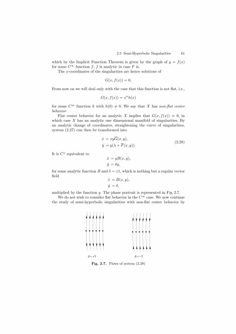
2.5 Semi-Hyperbolic Singularities 61
which by the Implicit Function Theorem is given by the graph of y = f(x)for some C∞ function f ; f is analytic in case F is.
The x-coordinates of the singularities are hence solutions of
G(x, f(x)) = 0.
From now on we will deal only with the case that this function is not flat, i.e.,
G(x, f(x)) = xnh(x)
for some C∞ function h with h(0) �= 0. We say that X has non-flat centerbehavior.
Flat center behavior for an analytic X implies that G(x, f(x)) ≡ 0, inwhich case X has an analytic one dimensional manifold of singularities. Byan analytic change of coordinates, straightening the curve of singularities,system (2.27) can then be transformed into
x = xyG(x, y),
y = y(λ + F (x, y)).(2.28)
It is Cω equivalent tox = yB(x, y),
y = δy,
for some analytic function B and δ = 1, which is nothing but a regular vectorfield
x = B(x, y),
y = δ,
multiplied by the function y. The phase portrait is represented in Fig. 2.7.We do not wish to consider flat behavior in the C∞ case. We now continue
the study of semi-hyperbolic singularities with non-flat center behavior by
d = +1 d = −1
Fig. 2.7. Flows of system (2.28)
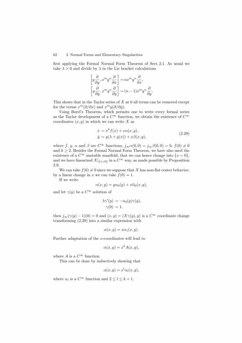
62 2 Normal Forms and Elementary Singularities
first applying the Formal Normal Form Theorem of Sect. 2.1. As usual wetake λ > 0 and divide by λ in the Lie bracket calculations
[y
∂
∂y, xmyn ∂
∂x
]=nxmyn ∂
∂x,
[y
∂
∂y, xmyn ∂
∂y
]= (n − 1)xmyn ∂
∂y.
This shows that in the Taylor series of X at 0 all terms can be removed exceptfor the terms xm(∂/∂x) and xmy(∂/∂y).
Using Borel’s Theorem, which permits one to write every formal seriesas the Taylor development of a C∞ function, we obtain the existence of C∞
coordinates (x, y) in which we can write X as
x = xkf(x) + xα(x, y),
y = y(λ + g(x)) + xβ(x, y),(2.29)
where f , g, α and β are C∞ functions, j∞α(0, 0) = j∞β(0, 0) = 0, f(0) �= 0and k ≥ 2. Besides the Formal Normal Form Theorem, we have also used theexistence of a C∞ unstable manifold, that we can hence change into {x = 0},and we have linearized X|{x=0} in a C∞ way, as made possible by Proposition2.9.
We can take f(0) �= 0 since we suppose that X has non-flat center behavior;by a linear change in x we can take f(0) = 1.
If we writeα(x, y) = yα0(y) + xα0(x, y),
and let γ(y) be a C∞ solution of
λγ′(y) = −α0(y)γ(y),
γ(0) = 1,
then j∞(γ(y) − 1)(0) = 0 and (x, y) = (Xγ(y), y) is a C∞ coordinate changetransforming (2.29) into a similar expression with
α(x, y) = xα1(x, y).
Further adaptation of the x-coordinates will lead to
α(x, y) = xkA(x, y),
where A is a C∞ function.This can be done by inductively showing that
α(x, y) = xlαl(x, y),
where αl is a C∞ function and 2 ≤ l ≤ k + 1.

2.5 Semi-Hyperbolic Singularities 63
We start with an expression
x = xkf(x) + xl(yαl(y) + xαl(x, y)),
y = y(λ + g(x)) + xβ(x, y),
for some 2 ≤ l ≤ k. By using the C∞ flat function
γ(y) = − 1
λ
∫ y
0
αl(u)du,
we find that (x + xlγ(y), y) are new C∞ variables for which X gets a similarexpression as (2.29) with
α(x, y) = xl+1αl+1(x, y)
for some C∞ function αl+1.As such, the expression that we get after the previous steps is
x = xk(f(x) + xA(x, y)),
y = y(λ + g(x)) + xB(x, y),(2.30)
where f , g, A and B are C∞ functions, j∞A(0, 0) = j∞B(0, 0) = g(0) = 0,f(0) = 1, k ≥ 2 and λ > 0.
We are now ready to prove the existence of (one or more) invariant C∞
manifolds that are tangent to the x-axis. Such an invariant manifold is calleda center manifold. We can represent it as the graph (x, y(x)) of a C∞ function,with y(0) = y′(0) = 0, and which is solution of the scalar differential equationrelated to (2.30) and having an expression
xk dy
dx= y(λ + h(x) + xC(x, y)) + xD(x, y), (2.31)
where h, C and D are C∞ functions, j∞C(0, 0) = j∞D(0, 0) = h(0) = 0,k ≥ 2 and λ > 0. We now study the required solutions of (2.31) in the nextlemma.
Lemma 2.11 Consider a scalar differential equation
xk dy
dx= y(λ + xF (x, y)) + G(x), (2.32)
where F and G are C∞ functions, j∞G(0) = 0 and λ �= 0. Then there isat least one C∞ solution y = α(x) with α : (−ε, ε) → R for some ε > 0sufficiently small, such that j∞α(0) = 0. Moreover, whenever β : (0, ε) → R
(respectively β : (−ε, 0) → R) is a solution, for some ε > 0, with limx→0
β(x) = 0,
then β : [0, ε) → R (respectively β : (−ε, 0] → R) defined by β(x) = β(x) forx �= 0 and β(0) = 0, is everywhere C∞ on its domain of definition andj∞β(0) = 0.
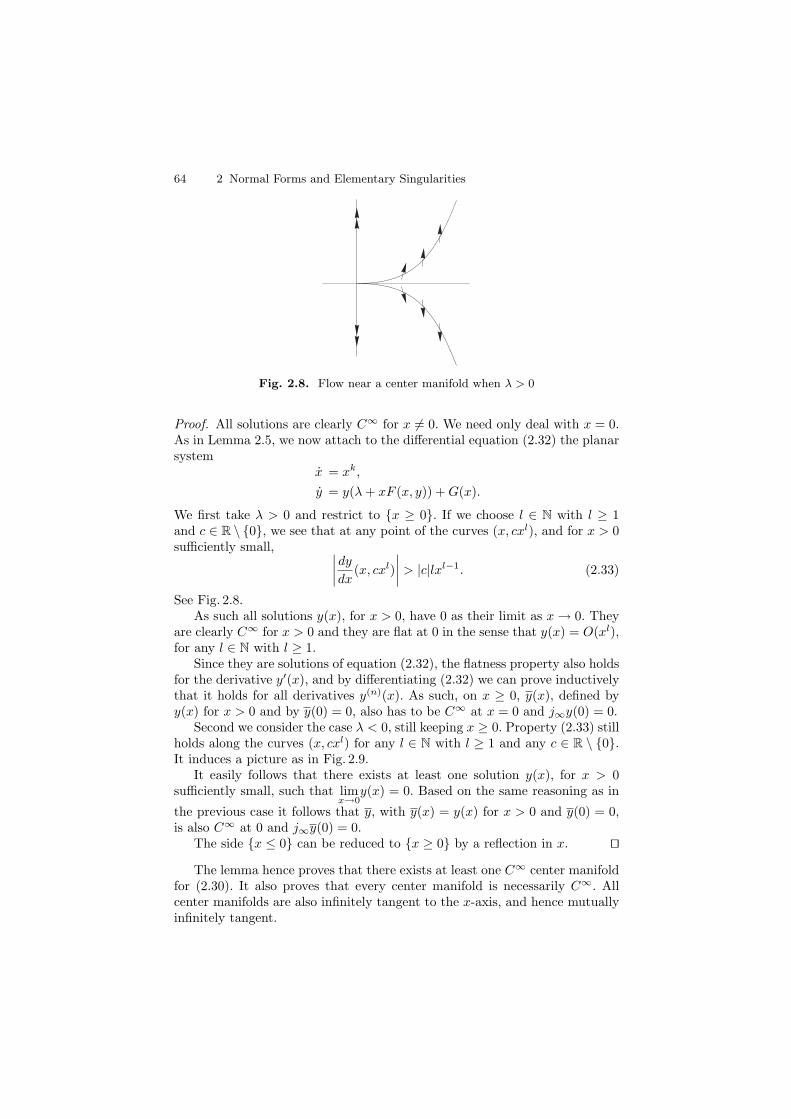
64 2 Normal Forms and Elementary Singularities
Fig. 2.8. Flow near a center manifold when λ > 0
Proof. All solutions are clearly C∞ for x �= 0. We need only deal with x = 0.As in Lemma 2.5, we now attach to the differential equation (2.32) the planarsystem
x = xk,
y = y(λ + xF (x, y)) + G(x).
We first take λ > 0 and restrict to {x ≥ 0}. If we choose l ∈ N with l ≥ 1and c ∈ R \ {0}, we see that at any point of the curves (x, cxl), and for x > 0sufficiently small, ∣∣∣∣
dy
dx(x, cxl)
∣∣∣∣ > |c|lxl−1. (2.33)
See Fig. 2.8.As such all solutions y(x), for x > 0, have 0 as their limit as x → 0. They
are clearly C∞ for x > 0 and they are flat at 0 in the sense that y(x) = O(xl),for any l ∈ N with l ≥ 1.
Since they are solutions of equation (2.32), the flatness property also holdsfor the derivative y′(x), and by differentiating (2.32) we can prove inductivelythat it holds for all derivatives y(n)(x). As such, on x ≥ 0, y(x), defined byy(x) for x > 0 and by y(0) = 0, also has to be C∞ at x = 0 and j∞y(0) = 0.
Second we consider the case λ < 0, still keeping x ≥ 0. Property (2.33) stillholds along the curves (x, cxl) for any l ∈ N with l ≥ 1 and any c ∈ R \ {0}.It induces a picture as in Fig. 2.9.
It easily follows that there exists at least one solution y(x), for x > 0sufficiently small, such that lim
x→0y(x) = 0. Based on the same reasoning as in
the previous case it follows that y, with y(x) = y(x) for x > 0 and y(0) = 0,is also C∞ at 0 and j∞y(0) = 0.
The side {x ≤ 0} can be reduced to {x ≥ 0} by a reflection in x. ⊓⊔
The lemma hence proves that there exists at least one C∞ center manifoldfor (2.30). It also proves that every center manifold is necessarily C∞. Allcenter manifolds are also infinitely tangent to the x-axis, and hence mutuallyinfinitely tangent.
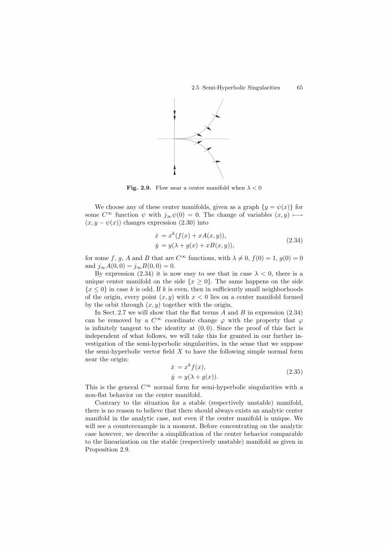
2.5 Semi-Hyperbolic Singularities 65
Fig. 2.9. Flow near a center manifold when λ < 0
We choose any of these center manifolds, given as a graph {y = ψ(x)} forsome C∞ function ψ with j∞ψ(0) = 0. The change of variables (x, y) �−→(x, y − ψ(x)) changes expression (2.30) into
x = xk(f(x) + xA(x, y)),
y = y(λ + g(x) + xB(x, y)),(2.34)
for some f , g, A and B that are C∞ functions, with λ �= 0, f(0) = 1, g(0) = 0and j∞A(0, 0) = j∞B(0, 0) = 0.
By expression (2.34) it is now easy to see that in case λ < 0, there is aunique center manifold on the side {x ≥ 0}. The same happens on the side{x ≤ 0} in case k is odd. If k is even, then in sufficiently small neighborhoodsof the origin, every point (x, y) with x < 0 lies on a center manifold formedby the orbit through (x, y) together with the origin.
In Sect. 2.7 we will show that the flat terms A and B in expression (2.34)can be removed by a C∞ coordinate change ϕ with the property that ϕis infinitely tangent to the identity at (0, 0). Since the proof of this fact isindependent of what follows, we will take this for granted in our further in-vestigation of the semi-hyperbolic singularities, in the sense that we supposethe semi-hyperbolic vector field X to have the following simple normal formnear the origin:
x = xkf(x),
y = y(λ + g(x)).(2.35)
This is the general C∞ normal form for semi-hyperbolic singularities with anon-flat behavior on the center manifold.
Contrary to the situation for a stable (respectively unstable) manifold,there is no reason to believe that there should always exists an analytic centermanifold in the analytic case, not even if the center manifold is unique. Wewill see a counterexample in a moment. Before concentrating on the analyticcase however, we describe a simplification of the center behavior comparableto the linearization on the stable (respectively unstable) manifold as given inProposition 2.9.
66 2 Normal Forms and Elementary Singularities
Proposition 2.12 Letu = uk(1 + g(u)), (2.36)
be a differential equation on R, where k ∈ N with k ≥ 2, g is a C∞ functionand g(0) = 0. Then there exists a change of coordinate
u = x(1 + α(x)), (2.37)
with α a C∞ function and α(0) = 0, changing (2.36) into
x = xk(1 + axk−1), (2.38)
for some a ∈ R. If g is analytic then α can be chosen to be analytic.
Proof. In fact we will not prove the proposition for the indicated normal form(2.38) but for the related one
x =xk
1 − axk−1. (2.39)
The latter result, of course, implies the required one. We will treat both theC∞ and the Cω results at once, each time writing C∞ (respectively Cω). Sowe start with an equation (2.36) where g is C∞ (respectively Cω). We write
g(u) =
N−1∑
i=1
aiui + O(uN ),
for some arbitrarily chosen N ≥ k. By inductively using a coordinate change
u = x(1 + αxl),
for a well chosen α, and 1 ≤ l ≤ k − 2, we can change g into
g(u) = auk−1 + O(uk).
The coefficient in front of uk−1 cannot be changed, but continuing the induc-tion on l we can, for each N > k, get
g(u) = auk−1 + O(uN ).
We can also adapt the power series of g in such a way that for (2.36) we get:
u =uk
1 − auk−1(1 + h(u)), (2.40)
where h is C∞ (respectively Cω) and h(u) = O(uN ). We leave this as anexercise, but take it now for granted.
We do not yet need to take a precise value for N , but we will see thatN ≥ 2k − 2 will permit us a proof of the proposition.

2.5 Semi-Hyperbolic Singularities 67
We now try a coordinate change
u = x(1 + y(x)), (2.41)
where y(x) is C∞ (respectively Cω), y(0) = 0, and check the necessary con-dition. Substituting (2.41) into (2.40) we immediately see that y needs to besolution of
(1 + y + xdy
dx) =
1 − axk−1
1 − axk−1(1 + y)k−1(1 + y)k(1 + O(xN )),
with O(xN ) some function in (x, y) which is C∞ (respectively Cω).A straightforward calculation reduces this to:
xdy
dx= y((k − 1) + A(x, y)) + B(x), (2.42)
where A and B are C∞ (respectively Cω functions), A(0, 0) = 0, B(x) =O(x2k−2).
If we write y = x2k−3Y , then (2.42) changes into
xdY
dx= Y ((2 − k) + A(x, x2k−3Y )) + C(x), (2.43)
for a function C which is C∞ (respectively Cω) and C(0) = 0.The differential equation (2.43) can be represented by the system
x = x,
Y = Y ((2 − k) + A(x, x2k−3Y )) + C(x).(2.44)
This system has a hyperbolic saddle at (0, 0) when k ≥ 3, while it has asemi-hyperbolic singularity for k = 2. In any case there exists a C∞ (re-spectively Cω) unstable manifold given by a graph (x, Y (x)). The functiony(x) = x2k−3Y (x) provides a solution of (2.42). ⊓⊔
Applying Proposition 2.12 to expression (2.35) we can put a semi-hyperbolicsingularity with non-flat center behavior in a very simple normal form for C∞-equivalence. We first multiply (2.35) by (λ + g(x))−1, leading to
x = xkf(x),
y = y,(2.45)
for some C∞ function f . We can require that f(0) = 1 by a linear coordinatechange. Applying Proposition 2.12 to xkf(x) we can change (2.45) into:
x = xk(1 + axk−1),
y = y.(2.46)
This is the final normal form for C∞ equivalence, in the sense that the coef-ficient a is an invariant if we want to keep the expression as it is.

68 2 Normal Forms and Elementary Singularities
d = +1 d = −1
Fig. 2.10. Saddle–nodes
2.5.2 Topological Results
Topological models, also for C0-conjugacy, are even simpler: there are threehyperbolic cases of, respectively, attracting, repelling and saddle type, besidesthe saddle-node type singularities
x = x2,
y = δy,
with δ = 1. See Fig. 2.10.We remark that it is a common practice, in representing local phase por-
traits of semi-hyperbolic singularities, to use double arrows for the flow on thestable/unstable invariant manifolds, and to use simple arrows on the centermanifold. This rule of double arrows is not always used when representingglobal phase portraits.
To prove our claim about topological models we start with the C∞ models(for C∞-conjugacy):
x = xk(1 + h(x)),
y = y(λ + g(x)),(2.47)
where h and g are C∞, h(0) = g(0) = 0 �= λ. The method of proof is acombination of the proofs employed in the topological study of the hyperbolicsingularities. The most delicate part deals with the monotonicity of the timefunction in the hyperbolic sectors. We study it on {x ≥ 0, y ≥ 0} for anexpression (2.47) with λ < 0. Without loss of generality we can take λ = −1.
We can also restrict to the calculation of the time that orbits spend be-tween sections C1 = {y = a} and C2 = {x = b} (see Fig. 2.11) with a > 0 andb > 0 and using the x-coordinate as a regular parameter on C1.
Along the orbits we have
dt =dx
xk(1 + h(x)).
So starting at a point (v, a), the time needed to arrive at {x = b} is given by
T (v) =
∫ b
v
dx
xk(1 + h(x)).
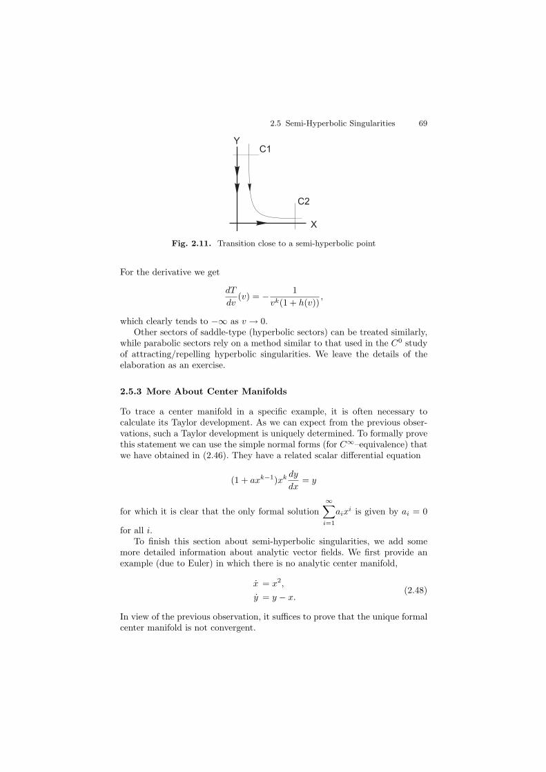
2.5 Semi-Hyperbolic Singularities 69
Fig. 2.11. Transition close to a semi-hyperbolic point
For the derivative we get
dT
dv(v) = − 1
vk(1 + h(v)),
which clearly tends to −∞ as v → 0.Other sectors of saddle-type (hyperbolic sectors) can be treated similarly,
while parabolic sectors rely on a method similar to that used in the C0 studyof attracting/repelling hyperbolic singularities. We leave the details of theelaboration as an exercise.
2.5.3 More About Center Manifolds
To trace a center manifold in a specific example, it is often necessary tocalculate its Taylor development. As we can expect from the previous obser-vations, such a Taylor development is uniquely determined. To formally provethis statement we can use the simple normal forms (for C∞–equivalence) thatwe have obtained in (2.46). They have a related scalar differential equation
(1 + axk−1)xk dy
dx= y
for which it is clear that the only formal solution
∞∑
i=1
aixi is given by ai = 0
for all i.To finish this section about semi-hyperbolic singularities, we add some
more detailed information about analytic vector fields. We first provide anexample (due to Euler) in which there is no analytic center manifold,
x = x2,
y = y − x.(2.48)
In view of the previous observation, it suffices to prove that the unique formalcenter manifold is not convergent.
70 2 Normal Forms and Elementary Singularities
To that end, consider a formal sum
y =
∞∑
n=1
ynxn,
such that y is a formal center manifold of (2.48), i.e.,
x2 dy
dx= y − x.
This equation leads to the easy recursion {nyn−yn+1, y1 = 1}. Hence yn = n!is the unique solution.
The formal expansion
y =
∞∑
n=1
n!xn,
is clearly divergent at all non-zero values of x.Although not convergent, the series in the example is not too divergent.
It is Gevrey-1 in x of type 1.
Definition 2.13 A formal power series
f(x) =
∞∑
n=0
fnxn,
is Gevrey-1/σ in x of type A if there exist positive constants A, C and α suchthat
|fn| ≤ CAn/σ Γ(α +
n
σ
),
for all n ≥ 0; Γ is the traditional gamma function.
For semi-hyperbolic singularities of analytic vector fields there is the fol-lowing result, which we state without proof.
Proposition 2.14 Let X be an analytic vector field having an expression(2.27) whose center behavior starts with the leading term xm, or more pre-cisely, such that
G(x, f(x)) = xm + o(xm).
Then there exists a unique formal center manifold y = f(x), and this uniqueformal power series is Gevrey-1/m in x of type m/|λ|.
The n th coefficient of a Gevrey-1/σ series is roughly of the order given by|Axσ|n/σ Γ (α+n/σ). It should be clear that for small |x|, the factor |An/σxn|competes against the factor Γ (α + n/σ). This explains the behavior of theupper bound: it is decreasing for small n, up to a point N(x), from which theupper bound rapidly tends to infinity. The order N(x) at which the upperbound is the smallest can be approximated, using Stirling’s formula, by

2.6 Summary on Elementary Singularities 71
N(x) =
[σ
A|x|σ]
,
(|Axσ|n/σ Γ(α + n/σ)
)n=N(x)
= O
(exp
(− 1
A|x|σ))
.
One can introduce now the notion of a Gevrey function: we say that a func-tion is Gevrey-1/σ asymptotic to a power series f if its N th order Taylor
development coincides with the N th order truncation fN of f , and if |f − fN |is of the order |Axσ|N/σ Γ(α + N/σ), for all N .
One can now approximate a function f by its N th order Taylor develop-ment, and by choosing the cut-off point equal to N(x), one finds an approxi-mation for which the error is exponentially small:
∣∣∣f(x) − fN(x)
∣∣∣ = O
(exp
(− 1
A|x|σ))
.
The finite sum fN(x) is called the summation to the least term.Let f be a function whose graph represents a center manifold of a vector
field of the earlier type. It is known that such a function is Gevrey-asymptoticto its formal counterpart. The approximation earlier is the best one can hopefor, and this is reflected in the fact that these center manifolds are in generalnon-unique and can differ by a function of the order O(exp(−1/A|x|σ)).
2.6 Summary on Elementary Singularities
Here we state two specific and practical theorems which summarize the pre-vious results and which are very helpful in determining the behavior of ele-mentary singular points.
We characterize the local phase portrait at a hyperbolic singular point inthe following theorem. Since we are mainly interested in polynomial differen-tial systems, we present the theorem for analytic systems.
Theorem 2.15 (Hyperbolic Singular Points Theorem) Let (0, 0) be anisolated singular point of the vector field X, given by
x = ax + by + A(x, y),y = cx + dy + B(x, y),
(2.49)
where A and B are analytic in a neighborhood of the origin with A(0, 0) =B(0, 0) = DA(0, 0) = DB(0, 0) = 0. Let λ1 and λ2 be the eigenvalues of thelinear part DX(0) of the system at the origin. Then the following statementshold.
(i) If λ1 and λ2 are real and λ1λ2 < 0, then (0, 0) is a saddle (see Fig. 2.12(a)).If we denote by E1 and E2 the eigenspaces of respectively λ1 and λ2, then

72 2 Normal Forms and Elementary Singularities
x x x x
y y y y
(b) (c) (d )(a)
Fig. 2.12. Phase portraits of non–degenerate singular points
one can find two invariant analytic curves, tangent respectively to E1 andE2 at 0, on one of which points are attracted towards the origin, and onone of which points are repelled away from the origin. On these invari-ant curves X is Cω-linearizable. There exists a C∞ coordinate changetransforming (2.49) into one of the following normal forms:
x = λ1x,
y = λ2y,
in the case λ2/λ1 ∈ R \ Q, and
x =x(λ1 + f(xkyl)),
y = y(λ2 + g(xkyl)),
in the case λ2/λ1 = −k/l ∈ Q with k, l ∈ N and where f and g are C∞
functions. All systems (2.49) are C0-conjugate to
x = x,
y = − y.
(ii) If λ1 and λ2 are real with |λ2| ≥ |λ1| and λ1λ2 > 0, then (0, 0) is anode (see Fig. 2.12(b)). If λ1 > 0 (respectively < 0) then it is repelling orunstable (respectively attracting or stable). There exists a C∞ coordinatechange transforming (2.49) into
x = λ1x,
y = λ2y,
in case λ2/λ1 /∈ N, and into
x = λ1x,
y = λ2y + δxm,
for some δ = 0 or 1, in case λ2 = mλ1 with m ∈ N and m ≥ 1. Allsystems (2.49) are C0-conjugate to
2.6 Summary on Elementary Singularities 73
x = δx,
y = δy,
with δ = 1 and λ1δ > 0.(iii) If λ1 = α+iβ and λ2 = α−iβ with α, β �= 0, then (0, 0) is a “strong” focus
(see Fig. 2.12(c)). If α > 0 (respectively < 0), it is repelling or unstable(respectively attracting or stable). There exists a C∞ coordinate changetransforming (2.49) into
x = αx + βy,
y = − βx + αy.
All systems (2.49) are C0-conjugate to
x = δx,
y = δy,
with δ = 1 and αδ > 0.(iv) If λ1 = iβ and λ2 = −iβ with β �= 0, then (0, 0) is a linear center,
topologically, a “weak” focus or a center (see Figs. 2.12(c) and (d)).
Remark 2.16 The proofs concerning the C∞- and C0-normal forms rely onthe results presented in Sect. 2.7 about the “removal of flat terms.” In fact wecould have given proofs of the C0 results not depending on it, but we decidednot to do so, since they can be found in many other texts.
Remark 2.17 The denomination strong focus in (iii) is used in describingsingularities of which the linear part DX(0) is already a focus, while thedenomination weak focus is used in the case DX(0) is a center. All resultspresented in this theorem are proven in this chapter (including Sect. 2.7),except for the last statement of (iv), namely that X is topologically a focus ora center. This proof will be given in Chap. 3. We added it here only for sakeof completeness.
Remark 2.18 The origin of system (2.49) is a hyperbolic singular point incases (i), (ii) and (iii) of Theorem 2.15.
Theorem 2.15 can also be stated in terms of the determinant (det), thetrace (tr) and the discriminant (dis) of the linear part at the singular point.Thus, statement (i) corresponds to det < 0; statement (ii) corresponds todet > 0, tr �= 0 and dis ≥ 0; statement (iii) corresponds to det > 0,tr �= 0 and dis < 0; and statement (iv) corresponds to det > 0, tr = 0and dis < 0.
We characterize the local phase portrait at a semi-hyperbolic singular pointin the following theorem, for whose proof we again rely on Sect. 2.7.
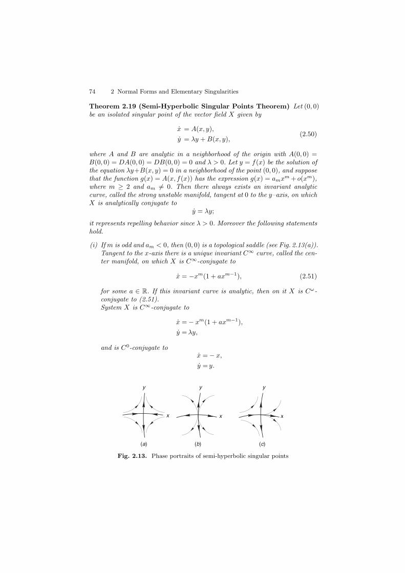
74 2 Normal Forms and Elementary Singularities
Theorem 2.19 (Semi-Hyperbolic Singular Points Theorem) Let (0, 0)be an isolated singular point of the vector field X given by
x = A(x, y),
y = λy + B(x, y),(2.50)
where A and B are analytic in a neighborhood of the origin with A(0, 0) =B(0, 0) = DA(0, 0) = DB(0, 0) = 0 and λ > 0. Let y = f(x) be the solution ofthe equation λy+B(x, y) = 0 in a neighborhood of the point (0, 0), and supposethat the function g(x) = A(x, f(x)) has the expression g(x) = amxm + o(xm),where m ≥ 2 and am �= 0. Then there always exists an invariant analyticcurve, called the strong unstable manifold, tangent at 0 to the y–axis, on whichX is analytically conjugate to
y = λy;
it represents repelling behavior since λ > 0. Moreover the following statementshold.
(i) If m is odd and am < 0, then (0, 0) is a topological saddle (see Fig. 2.13(a)).Tangent to the x-axis there is a unique invariant C∞ curve, called the cen-ter manifold, on which X is C∞-conjugate to
x = −xm(1 + axm−1), (2.51)
for some a ∈ R. If this invariant curve is analytic, then on it X is Cω-conjugate to (2.51).System X is C∞-conjugate to
x = − xm(1 + axm−1),
y = λy,
and is C0-conjugate tox = − x,
y = y.
x x x
y y y
(b) (c)(a)
Fig. 2.13. Phase portraits of semi-hyperbolic singular points
2.6 Summary on Elementary Singularities 75
(ii) If m is odd and am > 0, then (0, 0) is a unstable topological node (seeFig. 2.13(b)). Every point not belonging to the strong unstable manifoldlies on an invariant C∞ curve, called a center manifold, tangent to thex-axis at the origin, and on which X is C∞-conjugate to
x = xm(1 + axm−1), (2.52)
for some a ∈ R. All these center manifolds are mutually infinitely tangentto each other, and hence at most one of them can be analytic, in whichcase X is Cω-conjugate on it to (2.52).System X is C∞-conjugate to
x = xm(1 + axm−1),
y = λy,
and is C0-conjugate tox = x,
y = y.
(iii) If m is even, then (0, 0) is a saddle-node, that is, a singular point whoseneighborhood is the union of one parabolic and two hyperbolic sectors (seeFig. 2.13(c)). Modulo changing x into −x, we suppose that am > 0. Everypoint to the right of the strong unstable manifold (side x > 0) lies on aninvariant C∞ curve, called a center manifold, tangent to the x-axis at theorigin, and on which X is C∞-conjugate to
x = xm(1 + axm−1), (2.53)
for some a ∈ R. All these center manifolds coincide on the side x ≤ 0and are hence infinitely tangent at the origin. At most one of these centermanifolds can be analytic, in which case X is Cω-conjugate on it to (2.53).System X is C∞-conjugate to
x = xm(1 + axm−1),
y = λy,
and is C0-conjugate tox = x2,
y = y.
Remark 2.20 The case λ < 0 can be reduced to λ > 0 by changing Xinto −X. Besides the results on semi-hyperbolic singularities with non-flatcenter behavior, as stated in Theorem 2.19, we also recall that in case g(x) =A(x, f(x)), as defined in Theorem 2.19, is identically zero, then there existsan analytic curve consisting of singularities.
76 2 Normal Forms and Elementary Singularities
We leave it as an exercise to prove that, in that case, X is Cω-conjugateto
x = 0,
y = yh(x),
for some Cω function h with h(0) �= 0. It is hence Cω-equivalent to
x = 0,
y = δy,
with δ = 1.
2.7 Removal of Flat Terms
2.7.1 Generalities
In the previous sections we have left three problems concerning removal offlat terms in order to get the required C∞ normal forms. In each case wehave two C∞ vector fields X and X +Y , with the property that j∞Y (0) = 0;both vector fields are defined in a neighborhood of (0, 0). We want to finda local C∞ diffeomorphism ϕ : R2 → R2 with ϕ(0) = 0, ϕ∗X = Y andj∞(ϕ− I)(0, 0) = 0, for I the identity isomorphism; we call it a near-identitytransformation.
To that end we will use the so called homotopic method (see, e.g., [91]).We introduce a parameter τ ∈ [0, 1], consider Xτ = X + τY , and look for afamily ϕτ of near-identity transformations with the property that
(ϕτ )∗X = X + τY. (2.54)
It now suffices to look for a τ -dependent vector field Zτ with j∞(Zτ )(0, 0) =0 and satisfying
[X + τY, Zτ ] = Y, (2.55)
where [·, ·] denotes the usual Lie-bracket operation that we already used inSect. 2.1. We prove that this is sufficient in the next lemma, in which we usez = (x, y), Z(z, τ) = Zτ (z) and ϕ(z, τ) = ϕτ (z).
Lemma 2.21 Let Zτ be a solution to equation (2.55). Then ϕτ defined by
∂ϕ
∂τ(z, τ) = Z(ϕ(z, τ), τ), (2.56)
is a solution of equation (2.54).
Proof. It clearly follows from j∞(Zτ )(0, 0) = 0 that j∞(ϕ − I)(0, 0) = 0. Wefurthermore have to check condition (2.54), which we can write as

2.7 Removal of Flat Terms 77
⎛⎜⎝
∂ϕ1
∂x(z, τ)
∂ϕ1
∂y(z, τ)
∂ϕ2
∂x(z, τ)
∂ϕ2
∂y(z, τ)
⎞⎟⎠(
X1(z)X2(z)
)=
((X1 + τY1)(ϕ(z, τ)(X2 + τY2)(ϕ(z, τ)
). (2.57)
To find the relation with equation (2.55), we differentiate (2.57) with respectto τ
(Y1(ϕ(z, τ))Y2(ϕ(z, τ))
)=
⎛⎜⎝
∂
∂x(∂ϕ1
∂τ)(z, τ)
∂
∂y(∂ϕ1
∂τ)(z, τ)
∂
∂x(∂ϕ2
∂τ)(z, τ)
∂
∂y(∂ϕ2
∂τ)(z, τ)
⎞⎟⎠(
X1(z)X2(z)
)−
⎛⎜⎝
∂(X1 + τY1)
∂x(ϕ(z, τ))
∂(X1 + τY1)
∂y(ϕ(z, τ))
∂(X2 + τY2)
∂x(ϕ(z, τ))
∂(X2 + τY2)
∂y(ϕ(z, τ))
⎞⎟⎠
⎛⎜⎝
∂ϕ1
∂τ)(z, τ)
∂ϕ2
∂τ)(z, τ)
⎞⎟⎠ .
(2.58)
In this expression we can write
∂ϕi
∂τ(z, τ) = Zτ,i(ϕ(z, τ)), (2.59)
and by differentiating (2.59) we get
⎛⎜⎝
∂
∂x(∂ϕ1
∂τ)(z, τ)
∂
∂y(∂ϕ1
∂τ)(z, τ)
∂
∂x(∂ϕ2
∂τ)(z, τ)
∂
∂y(∂ϕ2
∂τ)(z, τ)
⎞⎟⎠ =
⎛⎜⎝
∂Zτ,1
∂x(ϕ(z, τ))
∂Zτ,1
∂y(ϕ(z, τ))
∂Zτ,2
∂x(ϕ(z, τ))
∂Zτ,2
∂y(ϕ(z, τ))
⎞⎟⎠
⎛⎜⎝
∂ϕ1
∂x(z, τ)
∂ϕ1
∂y(z, τ)
∂ϕ2
∂x(z, τ)
∂ϕ2
∂y(z, τ)
⎞⎟⎠ .
This relation, together with (2.57) and (2.59), shows that (2.58) is the sameas (2.55). As such (2.57) follows from (2.55) by integration, i.e., solving(2.56). ⊓⊔
Remark 2.22 If instead of having j∞Y (0, 0) = 0, we had only j∞Y (x, 0) = 0(respectively j∞Y (0, y) = 0), then clearly the “homotopic method” wouldimply that j∞(ϕ−I)(x, 0) = 0 (respectively j∞(ϕ−I)(0, y) = 0). It suffices inequation (2.55) to look for a solution which has the property that j∞Zτ (x, 0) =0 (respectively j∞Zτ (0, y) = 0).
Taking into account the previous remark, and knowing that we will needit in the sequel, we will from now on suppose that j∞Y (z) = 0 for all z ∈ M ,where M is either {(0, 0)}, {x = 0} or {y = 0}.
For solving (2.55) in the traditional way, it is important for X + τY to bea τ -family of complete vector fields, or at least, vector fields whose orbits existfor t → ∞. For the moment we take this for granted and denote the orbits by
78 2 Normal Forms and Elementary Singularities
γ(z, τ, t). We also suppose that, uniformly in τ ∈ [0, 1] and for initial values zin some ε-neighborhood of M , all orbits tend to M in an exponentially fastway
‖γ(z, τ, t)‖M ≤ Ce−λt‖z‖M , (2.60)
for some λ > 0, C > 0, and where ‖ · ‖M represents the distance to M . Undersome extra (rather mild) conditions, we will see that (2.55) can be solved bydefining
Zτ (z) = −∫ ∞
0
(F (γ(z, τ, t)))−1(Y (γ(z, τ, t)))dt for z /∈ M,
Zτ (z) = 0 for z ∈ M,
(2.61)
where F (γ(z, τ, t)) represents, along an orbit γ(z, τ, t), the matrix solution ofthe related variational equation
d
dtF (γ(z, τ, t)) = [Dz(X + τY )(γ(z, τ, t))](F (γ(z, τ, t))),
F (γ(z, τ, 0)) = I.(2.62)
From now on we suppose that Zτ is defined as in (2.61). In order to provethat Zτ is C∞, with j∞Zτ (z) = 0, for all z ∈ M , we will have to impose someextra conditions on X + τY . Once these conditions are proven, it is easy tocheck that Zτ satisfies the Lie-bracket relation required in (2.55), since (2.55)can clearly be written as
d
dt(Zτ (γ(z, τ, t))) = (Dz(X + τY )(γ(z, τ, t)))(Zτ (γ(z, τ, t))) + Y (γ(z, τ, t)),
from which it is clear that Zτ , as defined in (2.62), is a solution.To prove the smoothness of Zτ and the flatness at points z ∈ M , it will turn
out to be necessary to find good bounds on the norm of (F (γ(z, τ, t)))−1 aswell as on the norms of successive derivatives of (F (γ(z, τ, t)))−1 with respectto (z, τ). Since we know that
‖(F (γ(z, τ, t)))−1‖ =‖F (γ(z, τ, t))‖
|det(F (γ(z, τ, t)))| , (2.63)
it clearly shows that we essentially need to control the value of ‖F (γ(z, τ, t))‖and |det(F (γ(z, τ, t)))|. Upper bounds on ‖F (γ(z, τ, t))‖ will be obtainedfrom (2.62) by considering appropriate upper bounds on the expressionDz(X + τY )(γ(z, τ, t)). To find strictly positive lower bounds on the determi-nant |det(F (γ(z, τ, t)))| we will use Liouville’s formula stating that
|det(F (γ(z, τ, t)))| = exp
(∫ ∞
0
div(Dz(X + τY )(γ(z, τ, t)))dt
). (2.64)
This shows the importance that div(Dz(X + τY )(γ(z, τ, t))) has in this cal-culation. We now treat the specific cases encountered in the previous sectionsof this chapter.
2.7 Removal of Flat Terms 79
2.7.2 Hyperbolic Case
The simplest case is the attracting one, so we start with it.The divergence at (0, 0) is a strictly negative number, so on some neigh-
borhood V of the origin we can suppose that the divergence stays bounded,implying, in view of (2.64), the existence of some ν > 0 such that
|det(F (γ(z, τ, t)))| ≥ e−νt. (2.65)
Together with (2.62) this proves the existence of some μ > 0 with the propertythat
‖(F (γ(z, τ, t)))−1‖ ≤ eµt. (2.66)
Taking into account (2.60) with M = {(0, 0)}, and the fact that j∞Y (0, 0) = 0,we see at once that the integral in (2.61) converges and that
limz→(0,0)
Zτ (z) = 0.
Concerning the different derivatives (∂j+k+lZτ,i)/(∂xj∂yk∂τ l), we can ei-ther rely on uniform expressions of these derivatives (or their related tensors),or we can work inductively. In any case, from (2.62)–(2.64), and using the factthat Y is C∞ with j∞Y (0, 0), similar estimates as earlier will permit us toprove that Zτ is C∞ on V \ {(0, 0)} and that all derivatives tend to zero forz tending to the origin. We do not work it out, but leave it as an exercise. Inany case, the flatness at the origin of all derivatives implies that Zτ is alsoC∞ at the origin, with of course j∞Zτ (0, 0) = 0.
The repelling case can be reduced to the attracting one by reversing time,hence looking at −(X + τY ).
The treatment of the saddle case is more subtle, since we do not haveproperty (2.60) with respect to the origin. The idea now is to proceed in twosteps, relying on the following lemma that we state without proof. The proofcan be obtained by using a partition of unity in combination with a polarblow-up at the origin. We do not work this out but refer to [91].
Lemma 2.23 Let f : R2 → R be a C∞ function defined on a neighborhoodV of (0, 0) with j∞f(0) = 0. Then there is a decomposition f = g + h suchthat both g and h are C∞ functions on V with j∞g(p) = 0 and j∞h(q) = 0for all p = (x, 0) or q = (0, y) in V .
We consider a saddle point with expression (2.4) of Sect. 2.3, implying that{y = 0} represents the stable manifold while {x = 0} represents the unstableone.
Based on Lemma 2.23 we decompose the flat terms Y as Y = Ys +Yu withrespectively j∞Yu(x, 0) = 0 and j∞Ys(0, y) = 0 and we apply the homotopicmethod in order to subsequently remove Ys and Yu.
We start by removing Ys.
80 2 Normal Forms and Elementary Singularities
We recall that the family X + τY with Y = Ys has an expression
x = x(−λ1 + A(x, y) + τY1),
y = y(λ2 + B(x, y) + τY2),
with λ1 > 0, λ2 > 0, A(0, 0) = B(0, 0) = 0 and j∞Y1(0, y) = j∞Y2(0, y) = 0.We can chose a neighborhood V = V1 × V2 of the origin in which we have
−λ1 + A(x, y) + τY1 < −λ1
2.
We now consider a C∞ function α(y) with compact support inside V2 andequal to 1 in a neighborhood of 0. We change our focus to the study of
x =x(−λ1 + α(y)(A(x, y) + τY1)),
y = yα(y)(λ2 + B(x, y) + τY2).
For this vector field, it is clear that there exists an ε-neighborhood of M ={x = 0} on which not only all orbits exist for t → +∞, but also condition(2.60) holds with respect to M .
From now on it will be rather unimportant to know the exact behavior ofX + τY on M . So in view of an application of the same method to the semi-hyperbolic case, as we will do in the next subsection, we prove the followingproposition, which is of independent interest.
Proposition 2.24 Consider the differential equation
x =x(f(x, y) + τY1),
y = g(x, y) + τY2,(2.67)
on some ε-neighborhood V of M = {x = 0}, where f , g, Y1 and Y2 areC∞ functions and j∞Y1(0, y) = j∞Y2(0, y) = 0. Suppose moreover that g issupported in C×R for a compact set C ⊂ M , and that f(x, y)+τY1 < −λ < 0,for some λ > 0, τ ∈ [0, 1] and (x, y) ∈ V . Then the vector field Zτ , as definedin (2.61), with respect to X + τY as in (2.65), is a C∞ vector field satisfyingj∞Zτ (0, y) = 0 for all y.
Proof. The proof is essentially similar to the one we have given in studyingthe attracting hyperbolic case, i.e., M = {(0, 0)}. Of course, all estimatesneed to be made using ‖ · ‖M instead of ‖ · ‖, which is possible because of thefact that j∞Y1 and j∞Y2 are infinitely flat along M . Again the conditions on(2.67) imply that the divergence of X +τY stays bounded, implying condition(2.65) on |det(F (γ(z, τ, t)))| and condition (2.66) on ‖(F (γ(z, τ, t)))−1‖. Theproof is then completely analogous to the one in the case M = {(0, 0)} andwe leave it as an exercise. ⊓⊔
After removing Ys we can remove Yu in exactly the same way, by reversingtime and working with respect to M = {y = 0}.
2.7 Removal of Flat Terms 81
2.7.3 Semi-Hyperbolic Case
To remove flat terms in the semi-hyperbolic case, we start with the followingexpression for X
x = − xk(1 + f(x) + yw1(x, y)),
y = y(λ + g(x) + yw2(x, y)),(2.68)
where λ �= 0, f and g are C∞ functions and f(0) = g(0) = j∞w1(0, 0) =j∞w2(0, 0) = 0. We claim that there exists a C∞ near-identity change ofcoordinates at (0, 0) adapting (2.68) in a way that j∞wi(0, x) = 0 for i = 1, 2.In this way, the flat perturbation w = (w1, w2) can be considered to be flatalong {y = 0}. Since (2.68) is exponentially contracting towards {y = 0} (upto changing X into −X), Proposition 2.24 will permit us to completely removeit.
To prove the claim we work with Taylor expansions in y, having as coeffi-cients C∞ functions in x. The proof relies first on an induction procedure onthe powers of yn followed by an application of Borel’s Theorem for represent-ing such semi-formal developments by genuine C∞ functions in two variables(see for example [19] and [115]).
We now work out the induction procedure on n. Suppose that we can write(2.68) as
x = − xk(1 + f(x) + ynw1,n(x, y)),
y = y(λ + g(x) + ynw2,n(x, y)),(2.69)
for some n ≥ 1. We will now show how transformations of the form Id+O(yn)can change (2.69) into a similar expression with n replaced by n + 1.
We first try(x, y) = (X(1 + Xk−1ynα(X)), y), (2.70)
proving the existence of a flat C∞ function α(X) that permits us to changeynw1,n(x, y) into yn+1w1,n(X, y) for some C∞ function w1,n(X, y) such thatj∞w1,n(0, 0) = 0. We write fn(x) = w1,n(x, 0).
Substituting (2.70) into the first equation of (2.69), and writing x insteadof X, gives
x(1 + kxk−1ynα(x) + xkynα′(x)) + nxkyn−1α(x)y =
− xk(1 + xk−1ynα(x))k(1 + f(x(1 + xk−1ynα(x)))+
ynfn(x(1 + xk−1ynα(x))) + O(yn+1)).
Working modulo O(yn+1), this gives the following equation:
x(1 + kxk−1ynα(x) + xkynα′(x)) =
− xk[(1 + kxk−1ynα(x))(1 + f(x) + xkynα(x)f
′(x) + ynfn(x))+
nynα(x)(λ + g(x))] .
82 2 Normal Forms and Elementary Singularities
A straightforward calculation of the terms in yn shows that we have to solvethe following equation:
(1 + f(x))xkα′(x) = (n(λ + g(x)) + xkf′(x))α(x) + fn(x).
Seeing that j∞fn(0) = 0, Lemma 2.11 guarantees the existence of a C∞
solution α(x) with j∞α(0) = 0.Substituting (2.70) into the second equation of (2.69) does not change the
form of it.Coordinate change (2.70) hence reduces (2.69) to some expression
x = − xk(1 + f(x) + yn+1w1,n+1(x, y)),
y = y(λ + g(x) + yn+1w2,n+1(x, y)),(2.71)
of which we do not specify the relation with the previous expression, exceptfor the fact that the ∞-jet is unchanged.
Next we try(x, y) = (x, Y (1 + Y nβ(x)), (2.72)
proving the existence of a flat C∞ function β(x) that permits us to changeynw2,n(x, y) into Y n+1w2,n(x, Y ) for a convenient C∞ function w2,n such thatj∞w2,n(0, 0) = 0. We write gn(x) = w2,n(x, 0)
Substituting (2.72) into the second equation of (2.71), and writing y in-stead of Y , gives:
y(1 + (n + 1)ynβ(x)) + yn+1β′(x)x =
y(1 + ynβ(x))(λ + g(x) + yng(x) + O(yn+1)).
Working modulo O(yn+2) this gives the following equation:
y(1 + (n + 1)ynβ(x)) =
y(λ + g(x) + yngn(x) + (λ + g(x))ynβ(x) + ynβ′(x)xk(1 + f(x))).
A straightforward calculation of the terms in yn+1 shows that we have tosolve the following equation:
β′(x)xk(1 + f(x)) = n(λ + g(x))β(x) − gn(x).
Seeing that j∞gn(0) = 0, Lemma 2.11 guarantees the existence of a C∞
solution β(x) with j∞β(0) = 0.Substituting (2.72) into the first equation of (2.71) does not change its
form.The successive coordinate changes (2.70) and (2.72) prove that the induc-
tion works.We hence know that a semi-hyperbolic singularitiy is C∞-conjugate to
some normal form
2.7 Removal of Flat Terms 83
x = − xk(1 + f(x)),
y = y(λ + g(x)),(2.73)
We are now going to prove that two such normal forms are C∞-conjugateif they have the same formal development at (0, 0). We therefore consider
x = − xk(1 + f(x) + v1(x)),
y = y(λ + g(x) + v2(x)),(2.74)
with j∞v1(0) = j∞v2(0) = 0, and will show that (2.73) and (2.74) are mutu-ally C∞-conjugate.
We therefore first eliminate v1(x) by means of a coordinate change
(x, y) = (X(1 + α(X)), y). (2.75)
Substituting (2.75) into (2.74) and writing x instead of X gives
x(1 + α(x) + xα′(x)) = −xk(1 + α(x))k(1 + f(x(1 + α(x))))
leading to the equation
(1 + f(x) + v1(x))(1 + α(x) + xα′(x)) = (1 + α(x))k(1 + f(x(1 + α(x)))).
A straightforward calculation leads to
(1 + f(x) + v1(x))xα′(x) = ((k − 1) + O(x) + O(α(x)))α(x) − v1(x); (2.76)
by Lemma 2.6 and since j∞v1(0) = 0, we know that (2.76) has a C∞ solutionwith j∞α(0) = 0.
As such, the inverse transformation of (2.75) has changed (2.74) into
x = − xk(1 + f(x)),
y = y(λ + g(x) + w(x)),(2.77)
for some C∞ function w(x) with j∞w(0) = 0.We now consider the coordinate change
(x, y) = (x, Y (1 + β(x))). (2.78)
Substituting (2.78) into (2.77) and writing y instead of Y gives
y(1 + β(x)) + yβ′(x)x = y(1 + β(x))(λ + g(x) + w(x)).
This leads to
y(1 + β(x)) = y((1 + β(x))(λ + g(x) + w(x)) + (1 + f(x))xkβ′(x)).
A straightforward calculation gives
(1 + f(x))xkβ′(x) = −(1 + β(x))w(x),
which can be written as
(1 + f(x))β′(x) = −w(x)
xk(1 + β(x)).
This equation clearly has a C∞ solution with j∞β(0) = 0.
84 2 Normal Forms and Elementary Singularities
2.8 Exercises
Exercise 2.1 Find stable, unstable and center subspaces Es, Eu and Ec forthe linear systems given by the following matrices:
(2 −10 3
) (3 62 4
) (−3 62 −4
).
Exercise 2.2 Given the system x = x + 2y, y = y, show that there is aunique invariant regular C∞ curve through the origin.
Exercise 2.3 Suppose that X is a vector field on R2 with R∗(X) = X andX(0) = 0, where R(x, y) = (−x, y).
(i) Check all possible non-zero linear parts (1-jets) DX(0) of X at the origin.(ii)Give the formal normal form Y of j∞X(0), show that it also satisfies
R∗(Y ) = Y , and that it can be obtained by a coordinate change ϕ =Id + O(‖(x, y)‖2) such that ϕ ◦ R = R ◦ ϕ.
Exercise 2.4 For nilpotent singularities (i.e., X(0) = 0 and j1X(0) ∼y(∂/∂x)), we have found two interesting formal normal forms, namely
(y +
∞∑
i=2
aixi)
∂
∂x+ (
∞∑
j=2
bjxj)
∂
∂y
and
y∂
∂x+ (
∞∑
j=2
bjxj + y
∞∑
i=1
aixi)
∂
∂y.
Calculate the relation between (ai, bj) and (ai, bj).
Exercise 2.5 Given a formal power series∑∞
i=0 aixi, we know by Borel’s
Theorem that there exists a C∞ function f such that j∞f(0) =∑∞
i=0 aixi.
Show that such a C∞ function f is never uniquely determined.
Exercise 2.6 Check that for the inner product in expression (2.1) then(admAT ) = (admA)T indeed holds as claimed.
Exercise 2.7 Given a smooth two-dimensional vector field X such thatX(0) = 0 and DX(0) = A with A semi-simple (i.e., A is C-diagonalizable),show that there exists a formal normal form Y for X at 0 such that(etA)∗Y = Y for all t ∈ R.
2.8 Exercises 85
Exercise 2.8 Let X and Y be two-dimensional smooth vector fields withX(0) = Y (0) = 0 and let h be a local C0-conjugacy between X and Y at0, which is differentiable at the origin (Dh(0) exists). Show that DX(0) andDY (0) are linearly conjugate.
Hint: Use Exercise 1.1.
Exercise 2.9 Let X and Y be two-dimensional smooth vector fields withX(0) = Y (0) = 0. Suppose that X and Y are both hyperbolic attractors at0 with diagonal linear part and respective eigenvalues λ1 ≤ λ2 < 0 and μ1 ≤μ2 < 0. If X and Y are C0-equivalent at 0, by means of a homeomorphismh that it is differentiable at the origin (Dh(0) exists), then it can be proventhat λ1/λ2 = μ1/μ2. Show this in case λ1 = λ2.
Exercise 2.10 Show that the mapping h, defined in (2.2) and related toFig. 2.1, indeed defines a C0-conjugacy between X and L.
Exercise 2.11 Calculate a Taylor approximation of order 4 for the stableand unstable manifold of
x = 2x + 3x2 + 4xy + 6y3,
y = − y + x + 2x2 + 3xy2.
Exercise 2.12 Show that all vector fields (λ + εy)(∂/∂x) + λy(∂/∂y), for afixed λ ∈ R and variable ε �= 0, are mutually linearly conjugate.
Exercise 2.13 Prove the claim, made in the proof of Lemma 2.6 (seeFig. 2.2), that there exists at least one point on {x0} × [−y0, y0] whose ω-limit set is (0, 0).
Exercise 2.14 Solve next items:
(i) Prove the claim, made at the end of the proof of Lemma 2.6, that theproperty f(x) = O(xn), for every n ∈ N with n ≥ 1, also holds for thederivative f ′ of f .
(ii) Prove the same claim for all successive derivatives of f .(iii) Give an example of a C∞ function f on (0, 1) with f(x) = O(xn) for all
n ∈ N with n ≥ 1, but such that this property does not hold for f ′.
Exercise 2.15 Check in Sect. 2.4 (see Fig. 2.6) the details of the constructionof a C0-conjugacy between two hyperbolic saddles.
86 2 Normal Forms and Elementary Singularities
Exercise 2.16 Consider a C∞ vector field X = (X1, X2) defined on R2 andhaving both coordinate axes as invariant curves. Suppose that for X|{x≥0,y≥0}the following properties hold: X1(x, y) > 0 for x > 0, X2(x, y) < 0 for y > 0,(∂X2/∂y)(0, 0) < 0 and (∂X1/∂x)(0, 0) > 0. Let ϕ(p, t) denote the flow of X,with ϕ = (ϕ1, ϕ2). Show that for T > 0 sufficiently large there exists a uniquep ∈ {x ≥ 0, y ≥ 0} such that ϕ2(p, 0) = 1 and ϕ1(p, T ) = 1.
Exercise 2.17 Calculate a Taylor approximation of order 4 of the centermanifold of the following vector fields X at the origin:
(y + 2x + 3xy)∂
∂y+ (x2 + 2y2)
∂
∂x,
(3x3 + y3)∂
∂y+ (x + 4y3)
∂
∂x.
Also calculate in each of the foregoing cases the 3-jet of the center behaviorat the origin, i.e., the 3-jet at 0 of the vector field X|W c , where W c representsa C∞ center manifold.
Exercise 2.18 Calculate the precise expression of all possible center mani-folds at 0 for the following vector fields:
−y∂
∂y+x2 ∂
∂x,
−y∂
∂y−x3 ∂
∂x.
Exercise 2.19 Solve the exercise given in Remark 2.10.
Exercise 2.20 Let X be an analytic vector field on some open neighborhoodof (0, 0) in R2, having the origin as a non-isolated singularity and with theproperty that the divergence divX(0) �= 0.
(i) Show that X near the origin is Cω-conjugate to
x = 0
y = yh(x)
for some Cω function h with h(0) = 0.
Hint: Starting from (2.23), divide the vector field by y and use the flowbox theorem.
(ii) Show that X near the origin is Cω-equivalent to
x = 0
y = δy
with δ = 1.

2.8 Exercises 87
Exercise 2.21 Let X be a C∞ vector field on some open set U ⊂ R2, havingat some point p ∈ U a hyperbolic saddle with eigenvalues λ1 and λ2 satisfyingλ2/λ1 ∈ R \ Q. Show that if f : U → R is C∞ with Xf = 0 and f(p) = 0,then j∞f(p) = 0.
Exercise 2.22 Let X be a C∞ vector field on an open set U ⊂ R2, havingat p a hyperbolic saddle with eigenvalues λ1 and λ2 and such that λ2/λ1 ∈R \ Q. Show that there exists a neighborhood V of p in U and C∞ mappingsπs : V → W s, πu : V → Wu, with πs|W s = Id and πu|Wu = Id and withthe property that inside V both the foliations {π−1
s (y)} and {π−1u (x)} are
preserved under the flow of X, where x and y denote a regular parameter onrespectively the unstable and stable manifolds Wu and W s.
REMARK: The foliations {π−1s (y)} and {π−1
u (x)} are called invariant C∞
foliations.
Exercise 2.23 Let X be a C∞ vector field on an open set U ⊂ R2, havingat p a hyperbolic saddle with respectively W s and Wu as stable and unstablemanifolds. Suppose that there exist C∞ mappings πs : V → W s and πu :V → Wu with the properties described in the previous exercise. Show that Xnear p is (locally) C∞-linearizable.
REMARK: A similar technique can be used in any dimension to proveC∞-linearization of a hyperbolic saddle.
Exercise 2.24 Let U be an open subset of R2, let f : U → R be a Cr withr ≥ 2 function and let X(p) = ∇f(p) be the associated gradient vector fieldgiven by
x =∂f
∂x(x, y)
y =∂f
∂y(x, y).
Suppose that p is a singularity of X, then
(i) the eigenvalues of DX(p) are real.(ii)X has a hyperbolic singularity at p if and only if Df(p) = 0 and D2fp(·, ·)
is a non–degenerate bilinear form.
Exercise 2.25 Determine the Lyapunov stability and the asymptotic sta-bility (see Sect. 1.8) of the following list of singularities: hyperbolic saddle,hyperbolic focus, center, semi-hyperbolic singularity with non-flat centerbehavior.
88 2 Normal Forms and Elementary Singularities
Exercise 2.26 Let X1 and X2 be two C∞ vector fields having a hyperbolicsaddle at the origin. Then it is possible to prove that they are C0-equivalent,without using the monotonicity of the time function, as we did. One suchproof goes as follows:
(i) Use the existence of C∞ invariant stable and unstable manifolds to provethe existence of C∞ coordinates in which W s = {x = 0} and Wu = {y =0}.
(ii)Consider both X⊥i , where X⊥
i = gi(x, y)(∂/∂x) − fi(x, y)(∂/∂y) if Xi =fi(x, y) ∂
∂x + gi(x, y) ∂∂y .
Show that a mapping h is a C∞-equivalence between X1 and X2 on a neigh-borhood of (0, 0) if h is defined as follows:
(i) h|{x=0}∪{y=0} is the identity,(ii) h sends X1-orbits to X2-orbits,(iii) h sends X⊥
1 -orbits to X⊥2 -orbits,
(iv) for some y0 sufficiently small, let y = γi (x) denote the X⊥i -orbit with
γi (x) = y0. Then we require that h(x, γ1(x)) = (x, γ2(x)) for x in asufficiently small neighborhood of 0.
2.9 Bibliographical Comments
Although the idea of simplifying ordinary differential equations throughchanges of variables can already be found in earlier works, we can callPoincare the founding father of normal form theory as we use it nowadays.After Poincare the theory was developed by many people, among others Lya-punov, Dulac, Birkhoff, Siegel, Sternberg, Chen, Moser, Arnol’d, Pliss, Be-litskii, Bruno, Takens, Cushman, Sanders, Elphick, van der Meer, Yoccoz,Perez Marco and Stolovitch. In February 2005, MathSciNet provides 1618hits for “Normal forms” as element in the title. Maybe not all deal withdifferential equations, but many do. Some deal with formal aspects or withcomputational aspects. Others impose extra conditions on the normal formsor the normalizing transformations (like symmetries, preservation of extrastructure). Some deal with Cr normal forms, some with C∞ or analytic nor-mal forms, with individual vector fields or with families of vector fields. Tocite a few books, we mention in alphabetic order the books by Arnol’d [5],Arnol’d and Il’Yashenko [6], Bronstein and Kopanskii [21], Bruno [23], Chowand Hale [35], Chow, Li and Wang [36], Golubitsky and Schaeffer [74, 75],Guckenheimer and Holmes [77], Murdock [114] and Wiggins [164]. We alsowould like to mention the paper of Stowe [154] for many results concerningCs-linearization of resonant saddles, focusing on the problem of finding thebest s possible.
The theory of invariant manifolds also has a long history, although as withnormal form theory, it is still a very active branch of research. Introducing

2.9 Bibliographical Comments 89
“invariant manifold” on MathSciNet as element in the title gave 468 hits inFebruary 2005, besides another 144 with “invariant curve” in the title, 91 with“stable manifold,” 140 with “center manifold” and 42 with “centre manifold.”A number of these papers merely deal with the use of these objects but manydeal with more theoretical aspects.
Besides mentioning such names as Hadamard and Perron concerning thestable (and unstable) manifold, we want to mention the book of Hartman [80],as well as refer to some books that we have listed before concerning normalforms. We also cite the paper by Meyer [110] for the analyticity of theseobjects.
Concerning center manifolds we would like to refer to Carr [26], Fenichel[64], Kelley [96], Hirsch, Pugh and Shub [83], Sijbrand [149] and especially toVanderbauwhede [162], besides some of the books that we already mentionedearlier. We also want to refer to van Strien [161] for an example of a polynomialvector field not having a C∞ center manifold.
For a general introduction to the theory of dynamical systems, payingsignificant attention to normal forms and invariant manifolds, we can also referto Palis and de Melo [118], Robinson [136] and Katok and Hasselblatt [95].
The usual methods of proving results about normal forms and invariantmanifolds are somewhat different than the ones that we have used here. Ourchoice of proof is more elementary but is perhaps less appropriate for gener-alization to higher dimensions. For the two-dimensional case we believe thatit is quite complete in comparison to other texts since we not only prove theexistence of C∞ center manifolds, but also include good C∞ normal formsfor the elementary singularities. We also proved the existence of analytic sta-ble/unstable manifolds for elementary analytic singularities as well as goodanalytic normal forms on one dimensional analytic invariant manifolds. Thetheory of analytic normal forms for hyperbolic two-dimensional saddles ishowever beyond the scope of this book.

3
Desingularization of NonelementarySingularities
In this chapter we provide the basic tool for studying nonelementary singu-larities of a differential system in the plane. This tool is based on changes ofvariables called blow-ups. We use this technique for classifying the nilpotentsingularities; i.e., the singularities having both eigenvalues zero but whose lin-ear part is not identically zero. Blow-up is also used to show that at isolatedsingularities an analytic system has a finite sectorial decomposition.
3.1 Homogeneous Blow-Up
Before describing the effective algorithm that we use in the program P4 [9],and which is based on the use of quasihomogeneous blow-up, we will first ex-plain the basic ideas only introducing homogeneous blow-up, which essentiallymeans using polar coordinates. We position the singularity that we want tostudy at the origin.
Let 0 be a singularity of a C∞ vector field X on R2. Consider the map
φ : S1 × R → R2
(θ, r) �→ (r cos θ, r sin θ) .
We can define a C∞ vector field X on the cylinder S1 × R such thatφ∗(X) = X, in the sense that Dφv(X(v)) = X(φ(v)). It is called the pullback of X by φ. It is nothing else but X written down in polar coordinates.The map φ is a C∞ diffeomorphism, hence a genuine C∞ coordinate changeon S1 × (0,∞), but not on {r = 0}; φ sends {r = 0} to (0, 0), and as such,the inverse mapping φ−1 blows up the origin to a circle. In order to studythe phase portrait of X in a neighborhood V of the origin, it clearly sufficesto study the phase portrait of X on the neighborhood φ−1(V ) of the circleS1×{0}, and we can even restrict to {r ≥ 0}. A priori this might seem a moredifficult problem than the original one, but as we will see in this chapter, theconstruction is very helpful. If the k-jet jk(X)(0) is zero, then jk(X)(u) = 0for all u ∈ S1 × {0}.
92 3 Desingularization of Nonelementary Singularities
Although the cylinder is a good surface for getting a global view of X andits phase portrait, it is often less appropriate for making calculations, sincewe constantly have to deal with trigonometric expressions. For that reason itis often preferable to make the calculations in different charts.
On the parts of the cylinder given, respectively, by θ ∈ (−π/2, π/2) andθ ∈ (π/2, 3π/2) use a chart given by
Kx : (θ, r) �→ (r cos θ, tan θ) = (x, y).
In this chart the expression of the blow-up map φ is given by
φx : (x, y) �→ (x, xy). (3.1)
Indeed we see that
φ = φx ◦ Kx : (θ, r)Kx
�→(r cos θ, tan θ)
φx
�→(r cos θ, r cos θ tan θ) = (r cos θ, r sin θ).(3.2)
We call (3.1) a “blow-up in the x-direction”; the pull-back of X by means ofφx is denoted by Xx, i.e., (φx)∗(Xx) = X.
On the parts of the cylinder given, respectively, by θ ∈ (0, π) and θ ∈(π, 2π), we use a chart given by
Ky : (θ, r) �→ (cot θ, r sin θ) = (x, y).
In this chart the expression of the blow-up map φ is given by
φy : (x, y) �→ (xy, y), (3.3)
in the sense that φ = φy ◦ Ky. We call (3.3) a “blow-up in the y–direction”;the pullback of X by means of φy is denoted by Xy, i.e., (φy)∗(Xy) = X.
Both φx and φy are called “directional blow-ups.”If jk(X)(0) = 0 and jk+1(X)(0) �= 0, then again jk(Xx)(z) = 0 and
jk(Xy)(z) = 0 for, respectively, z ∈ {x = 0} or z ∈ {y = 0}.In case jk(X)(0) = 0 and jk+1(X)(0) �= 0 the pullback X and likewise Xx
and Xy, are quite degenerate, and to make the situation less degenerate weconsider X with
X =1
rkX.
Then X also is a C∞ vector field on S1×R. On {r > 0} this division does notchange the orbits of X or their sense of direction, but only the parametrizationby t. From the formulas it is clear that singularities of X|{r = 0} come in pairsof opposite points.
For the related directional blow-up we use (1/xk)Xx in case (3.1) and(1/yk)Xy in case (3.3). On {x �= 0} (respectively {y �= 0}) the vector fields
3.1 Homogeneous Blow-Up 93
(1/rk)X and (1/xk)Xx (respectively (1/yk)Xy) are no longer equal up toanalytic coordinate change, as were X and Xx (respectively, Xy), but theyare the same up to analytic coordinate change and multiplication by a nonzeroanalytic function.
We work this out for the blow-up in the x-direction: since φ = φx ◦ Kx,we see that (Kx)∗(X) = Xx.
As such
(Kx)∗(X) = (Kx)∗(X/rk) =1
rk(Kx)∗(X) =
1
rkXx = X
x(x
r)k.
Seen in (θ, r)-coordinates we have x/r = cos θ, which is strictly positiveon the part of the cylinder given by θ ∈ (−π/2, π/2).
Similarly in the y-direction, we have (Ky)∗(X) = Xy and (Ky)∗(X) =X
y(sin θ)k, with sin θ > 0 on the part of the cylinder given by θ ∈ (0, π).The directional blow-up φx can also be used for making a study on {(θ, r) :
θ ∈ (π/2, 3π/2), r ≥ 0}, but in that case we have cos θ < 0.For odd k, this means that in the phase portraits that we find for X
x|{x≤0}we have to reverse time. A similar observation has to be made in using X
y
for studying X on {(θ, r) : θ ∈ (π, 2π), r > 0}.Such a time reversal could be avoided in using φx (respectively, φy) only
for x ≥ 0 (respectively, y ≥ 0), and adding two extra directional blow-ups
φ−x : (x, y) �→ (−x,−xy),
φ−y : (x, y) �→ (−xy,−y),
that we limit to, respectively, x ≥ 0 and y ≥ 0. Of course the number ofcalculations can be limited by using both φx and φy on a full neighborhoodof, respectively, {x = 0} and {y = 0}, avoiding having to work with φ−x andφ−y.
We now treat a few examples.
Example 3.1 First we present an example in which we use one blow-upto obtain quite easily the topological picture of the orbit structure of thesingularity:
X = (x2 − 2xy)∂
∂x+ (y2 − xy)
∂
∂y+ O(‖(x, y)‖3).
The formulas for (polar) blow-up are
X = η1∂
∂θ+ η2r
∂
∂r,

94 3 Desingularization of Nonelementary Singularities
with
η1(θ, r) =1
rk+2
⟨X,x
∂
∂y− y
∂
∂x
⟩(φ(r, θ))
=1
rk+2(−r sin θX1(r cos θ, r sin θ) + r cos θX2(r cos θ, r sin θ)),
η2(θ, r) =1
rk+2
⟨X,x
∂
∂x+ y
∂
∂y
⟩(φ(r, θ))
=1
rk+2(r cos θX1(r cos θ, r sin θ) + r sin θX2(r cos θ, r sin θ)),
In our example k = 1 and the result is
X(θ, r) = (cos θ sin θ(3 sin θ − 2 cos θ) + O(r))∂
∂θ
+ r(cos3 θ − 2 cos2 θ sin θ − cos θ sin2 θ + sin3 θ + O(r))∂
∂r.
Zeros on {r = 0} are located at
θ = 0, π; θ = π/2, 3π/2; tan θ = 2/3.
At these singularities, the radial eigenvalue is given by the coefficient of r∂/∂rwhile the tangential eigenvalue can be found by differentiating the ∂/∂θ-component with respect to θ. One thus obtains Fig. 3.1. In this figure werepresent the half cylinder S1 × [0,∞) as E = {(x, y) : x2 + y2 ≥ 1}. Thisvisualization will also be used in the sequel. The phase portrait which wesee on E near the circle C = {x2 + y2 = 1} gives a very good idea of thephase portrait of X near the origin. It suffices to shrink the circle to a point(see Fig. 3.2).
All the singularities on S1 × {0} are hyperbolic. We say that we havedesingularized X at 0 since all singularities of X|{r=0} are elementary. The
Fig. 3.1. Blow-up of Example 3.1
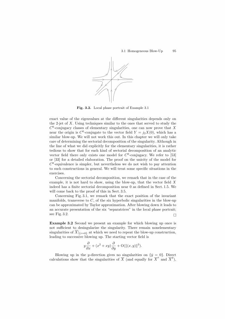
3.1 Homogeneous Blow-Up 95
Fig. 3.2. Local phase portrait of Example 3.1
exact value of the eigenvalues at the different singularities depends only onthe 2-jet of X. Using techniques similar to the ones that served to study theC0-conjugacy classes of elementary singularities, one can now prove that Xnear the origin is C0-conjugate to the vector field Y = j2X(0), which has asimilar blow-up. We will not work this out. In this chapter we will only takecare of determining the sectorial decomposition of the singularity. Although inthe line of what we did explicitly for the elementary singularities, it is rathertedious to show that for each kind of sectorial decomposition of an analyticvector field there only exists one model for C0-conjugacy. We refer to [53]or [33] for a detailed elaboration. The proof on the unicity of the model forC0-equivalence is simpler, but nevertheless we do not wish to pay attentionto such constructions in general. We will treat some specific situations in theexercises.
Concerning the sectorial decomposition, we remark that in the case of theexample, it is not hard to show, using the blow-up, that the vector field Xindeed has a finite sectorial decomposition near 0 as defined in Sect. 1.5. Wewill come back to the proof of this in Sect. 3.5.
Concerning Fig. 3.1, we remark that the exact position of the invariantmanifolds, transverse to C, of the six hyperbolic singularities in the blow-upcan be approximated by Taylor approximation. After blowing down it leads toan accurate presentation of the six “separatrices” in the local phase portrait;see Fig. 3.2.
Example 3.2 Second we present an example for which blowing up once isnot sufficient to desingularize the singularity. There remain nonelementarysingularities of X|{r=0} at which we need to repeat the blow-up construction,leading to successive blowing up. The starting vector field is
y∂
∂x+ (x2 + xy)
∂
∂y+ O(‖(x, y)‖3).
Blowing up in the y-direction gives no singularities on {y = 0}. Directcalculations show that the singularities of X (and equally for X
xand X
y),

96 3 Desingularization of Nonelementary Singularities
as well as their eigenvalues, depend only on the first nonzero jet, hence ony∂/∂x in this example. We now perform a blow-up in the x-direction, workingout the calculations explicitly. Writing
x = x, y = xy,
orx = x, y = y/x,
we get
˙x = x
= y + O(‖(x, y)‖3)
= yx + O(|x|3),
˙y =y
x− y
x
x2
= (x + y) +1
xO(‖(x, y)‖3) − y2
x2− y
x2O(‖(x, y)‖3)
= x + y x − y2 + O(|x|2).
(3.4)
The only singularity on x = 0 occurs for y = 0, where the 1-jet of the vectorfield Xx at this singularity is x∂/∂y.
As the singularity is nonelementary, we are going to perform an extra blow-up in order to study it. Blowing up in the x-direction gives no singularities.Blowing up (3.4) in the y-direction (x = ¯y ¯x, y = ¯y) gives
˙y = ˙y
= (x + y x − y2 + O(|x|2))= ¯x ¯y − ¯y2 + O(‖(¯x, ¯y)‖3),
˙x =˙x
y− x
˙y
y2
= x +1
yO(|x|3) − x
y2(x + yx − y2 + O(|x|2))
= ¯y ¯x − ¯x2 + ¯y ¯x + O(‖(¯x, ¯y)‖2).
The 2-jet is now (¯x¯y − ¯y2)∂/∂ ¯y + (2¯x¯y − ¯x2)∂/∂ ¯x. This singularity is notelementary, but as we have seen in Example 3.1, it can be studied by blowingup once. This succession of blowing up is schematized in Fig. 3.3. At eachstep we blow-up a point to a circle, not forgetting that singularities of X on{r = 0} always come in pairs of opposite points. If we need to blow-up one, wealso apply the same blow-up procedure to the second. As we already observedin discussing the directional blow-up X
xand X
yin relation to X, the study
of both singularities at a pair of opposite points can be done on the sameexpressions by treating x ≤ 0 as well as x ≥ 0, or, respectively, y ≤ 0 as well
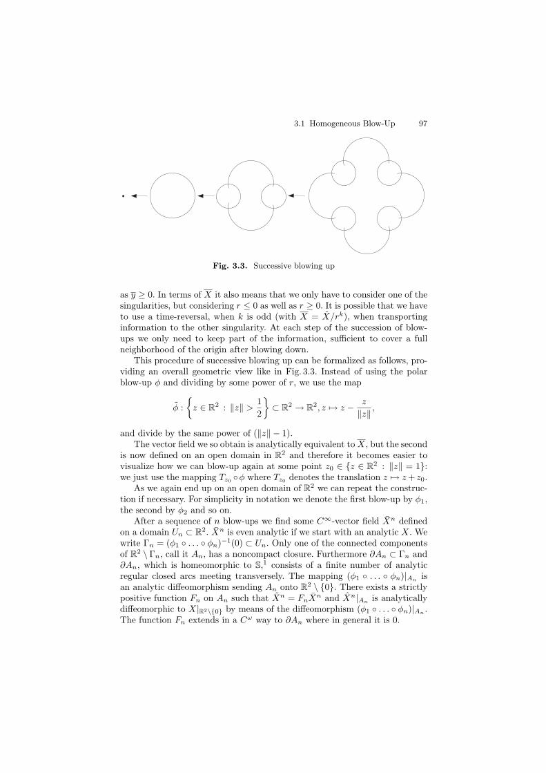
3.1 Homogeneous Blow-Up 97
Fig. 3.3. Successive blowing up
as y ≥ 0. In terms of X it also means that we only have to consider one of thesingularities, but considering r ≤ 0 as well as r ≥ 0. It is possible that we haveto use a time-reversal, when k is odd (with X = X/rk), when transportinginformation to the other singularity. At each step of the succession of blow-ups we only need to keep part of the information, sufficient to cover a fullneighborhood of the origin after blowing down.
This procedure of successive blowing up can be formalized as follows, pro-viding an overall geometric view like in Fig. 3.3. Instead of using the polarblow-up φ and dividing by some power of r, we use the map
φ :
{z ∈ R2 : ‖z‖ >
1
2
}⊂ R2 → R2, z �→ z − z
‖z‖ ,
and divide by the same power of (‖z‖ − 1).The vector field we so obtain is analytically equivalent to X, but the second
is now defined on an open domain in R2 and therefore it becomes easier tovisualize how we can blow-up again at some point z0 ∈ {z ∈ R2 : ‖z‖ = 1}:we just use the mapping Tz0
◦φ where Tz0denotes the translation z �→ z + z0.
As we again end up on an open domain of R2 we can repeat the construc-tion if necessary. For simplicity in notation we denote the first blow-up by φ1,the second by φ2 and so on.
After a sequence of n blow-ups we find some C∞-vector field Xn definedon a domain Un ⊂ R2. Xn is even analytic if we start with an analytic X. Wewrite Γn = (φ1 ◦ . . . ◦ φn)−1(0) ⊂ Un. Only one of the connected componentsof R2 \ Γn, call it An, has a noncompact closure. Furthermore ∂An ⊂ Γn and∂An, which is homeomorphic to S,1 consists of a finite number of analyticregular closed arcs meeting transversely. The mapping (φ1 ◦ . . . ◦ φn)|An
isan analytic diffeomorphism sending An onto R2 \ {0}. There exists a strictlypositive function Fn on An such that Xn = FnXn and Xn|An
is analyticallydiffeomorphic to X|R2\{0} by means of the diffeomorphism (φ1 ◦ . . . ◦ φn)|An
.The function Fn extends in a Cω way to ∂An where in general it is 0.
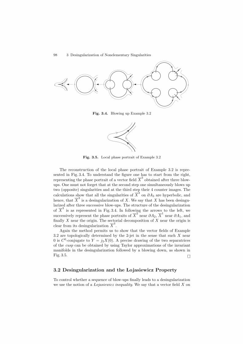
98 3 Desingularization of Nonelementary Singularities
Fig. 3.4. Blowing up Example 3.2
Fig. 3.5. Local phase portrait of Example 3.2
The reconstruction of the local phase portrait of Example 3.2 is repre-sented in Fig. 3.4. To understand the figure one has to start from the right,
representing the phase portrait of a vector field X3
obtained after three blow-ups. One must not forget that at the second step one simultaneously blows uptwo (opposite) singularities and at the third step their 4 counter images. The
calculations show that all the singularities of X3
on ∂A3 are hyperbolic, and
hence, that X3
is a desingularization of X. We say that X has been desingu-larized after three successive blow-ups. The structure of the desingularization
of X3
is as represented in Fig. 3.4. In following the arrows to the left, we
successively represent the phase portraits of X2
near ∂A2, X1
near ∂A1, andfinally X near the origin. The sectorial decomposition of X near the origin is
clear from its desingularization X3.
Again the method permits us to show that the vector fields of Example3.2 are topologically determined by the 2-jet in the sense that such X near0 is C0-conjugate to Y = j2X(0). A precise drawing of the two separatricesof the cusp can be obtained by using Taylor approximations of the invariantmanifolds in the desingularization followed by a blowing down, as shown inFig. 3.5.
3.2 Desingularization and the �Lojasiewicz Property
To control whether a sequence of blow-ups finally leads to a desingularizationwe use the notion of a �Lojasiewicz inequality. We say that a vector field X on
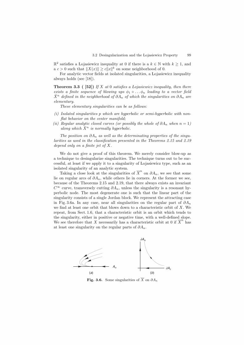
3.2 Desingularization and the �Lojasiewicz Property 99
R2 satisfies a �Lojasiewicz inequality at 0 if there is a k ∈ N with k ≥ 1, anda c > 0 such that ‖X(x)‖ ≥ c‖x‖k on some neighborhood of 0.
For analytic vector fields at isolated singularities, a �Lojasiewicz inequalityalways holds (see [18]).
Theorem 3.3 ( [52]) If X at 0 satisfies a �Lojasiewicz inequality, then thereexists a finite sequence of blowing ups φ1 ◦ . . . φn leading to a vector fieldXn defined in the neighborhood of ∂An of which the singularities on ∂An areelementary.
These elementary singularities can be as follows:
(i) Isolated singularities p which are hyperbolic or semi-hyperbolic with non-flat behavior on the center manifold;
(ii) Regular analytic closed curves (or possibly the whole of ∂An when n = 1)along which Xn is normally hyperbolic.
The position on ∂An as well as the determinating properties of the singu-larities as used in the classification presented in the Theorems 2.15 and 2.19depend only on a finite jet of X.
We do not give a proof of this theorem. We merely consider blow-up asa technique to desingularize singularities. The technique turns out to be suc-cessful, at least if we apply it to a singularity of �Lojasiewicz type, such as anisolated singularity of an analytic system.
Taking a close look at the singularities of Xn
on ∂An, we see that somelie on regular arcs of ∂An, while others lie in corners. At the former we see,because of the Theorems 2.15 and 2.19, that there always exists an invariantC∞ curve, transversely cutting ∂An, unless the singularity is a resonant hy-perbolic node. The most degenerate one is such that the linear part of thesingularity consists of a single Jordan block. We represent the attracting casein Fig. 3.6a. In any case, near all singularities on the regular part of ∂An
we find at least one orbit that blows down to a characteristic orbit of X. Werepeat, from Sect. 1.6, that a characteristic orbit is an orbit which tends tothe singularity, either in positive or negative time, with a well-defined slope.We see therefore that X necessarily has a characteristic orbit at 0 if X
nhas
at least one singularity on the regular parts of ∂An.
(a) (b)
∂An
∂AnAn
Fig. 3.6. Some singularities of X on ∂An
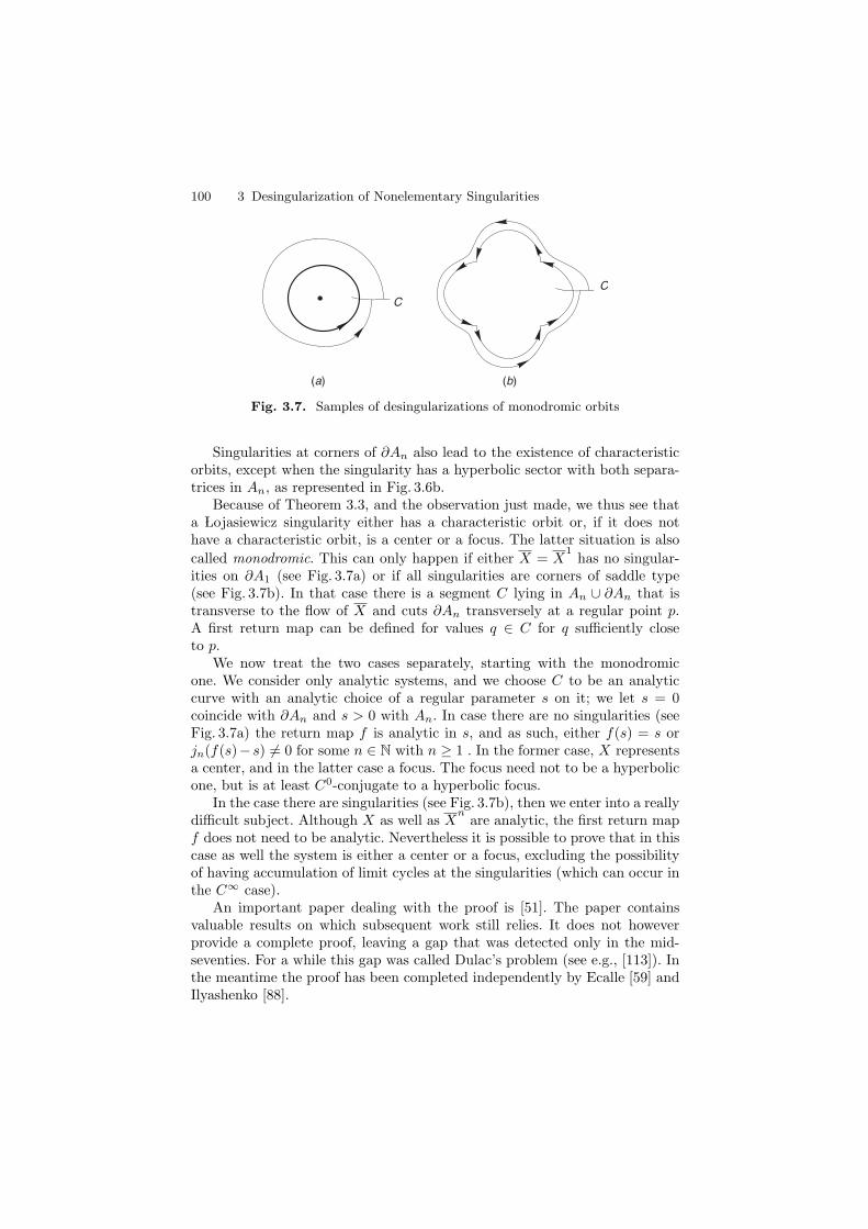
100 3 Desingularization of Nonelementary Singularities
C
(a)
C
(b)
Fig. 3.7. Samples of desingularizations of monodromic orbits
Singularities at corners of ∂An also lead to the existence of characteristicorbits, except when the singularity has a hyperbolic sector with both separa-trices in An, as represented in Fig. 3.6b.
Because of Theorem 3.3, and the observation just made, we thus see thata �Lojasiewicz singularity either has a characteristic orbit or, if it does nothave a characteristic orbit, is a center or a focus. The latter situation is also
called monodromic. This can only happen if either X = X1
has no singular-ities on ∂A1 (see Fig. 3.7a) or if all singularities are corners of saddle type(see Fig. 3.7b). In that case there is a segment C lying in An ∪ ∂An that istransverse to the flow of X and cuts ∂An transversely at a regular point p.A first return map can be defined for values q ∈ C for q sufficiently closeto p.
We now treat the two cases separately, starting with the monodromicone. We consider only analytic systems, and we choose C to be an analyticcurve with an analytic choice of a regular parameter s on it; we let s = 0coincide with ∂An and s > 0 with An. In case there are no singularities (seeFig. 3.7a) the return map f is analytic in s, and as such, either f(s) = s orjn(f(s)− s) �= 0 for some n ∈ N with n ≥ 1 . In the former case, X representsa center, and in the latter case a focus. The focus need not to be a hyperbolicone, but is at least C0-conjugate to a hyperbolic focus.
In the case there are singularities (see Fig. 3.7b), then we enter into a reallydifficult subject. Although X as well as X
nare analytic, the first return map
f does not need to be analytic. Nevertheless it is possible to prove that in thiscase as well the system is either a center or a focus, excluding the possibilityof having accumulation of limit cycles at the singularities (which can occur inthe C∞ case).
An important paper dealing with the proof is [51]. The paper containsvaluable results on which subsequent work still relies. It does not howeverprovide a complete proof, leaving a gap that was detected only in the mid-seventies. For a while this gap was called Dulac’s problem (see e.g., [113]). Inthe meantime the proof has been completed independently by Ecalle [59] andIlyashenko [88].
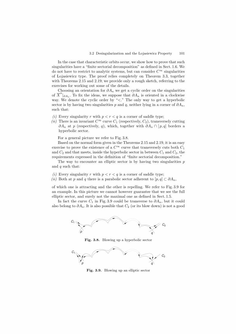
3.2 Desingularization and the �Lojasiewicz Property 101
In the case that characteristic orbits occur, we show how to prove that suchsingularities have a “finite sectorial decomposition” as defined in Sect. 1.6. Wedo not have to restrict to analytic systems, but can consider C∞ singularitiesof �Lojasiewicz type. The proof relies completely on Theorem 3.3, togetherwith Theorems 2.15 and 2.19; we provide only a rough sketch, referring to theexercises for working out some of the details.
Choosing an orientation for ∂An we get a cyclic order on the singularitiesof X
n|∂An. To fix the ideas, we suppose that ∂An is oriented in a clockwise
way. We denote the cyclic order by “<.” The only way to get a hyperbolicsector is by having two singularities p and q, neither lying in a corner of ∂An,such that:
(i) Every singularity r with p < r < q is a corner of saddle type;(ii) There is an invariant C∞ curve C1 (respectively, C2), transversely cutting
∂An at p (respectively, q), which, together with ∂An ∩ [ p, q] borders ahyperbolic sector.
For a general picture we refer to Fig. 3.8.Based on the normal form given in the Theorems 2.15 and 2.19, it is an easy
exercise to prove the existence of a C∞ curve that transversely cuts both C1
and C2 and that meets, inside the hyperbolic sector in between C1 and C2, therequirements expressed in the definition of “finite sectorial decomposition.”
The way to encounter an elliptic sector is by having two singularities pand q such that:
(i) Every singularity r with p < r < q is a corner of saddle type;(ii) Both at p and q there is a parabolic sector adherent to [p, q] ⊂ ∂An,
of which one is attracting and the other is repelling. We refer to Fig. 3.9 foran example. In this picture we cannot however guarantee that we see the fullelliptic sector, and surely not the maximal one as defined in Sect. 1.5.
In fact the curve C1 in Fig. 3.9 could be transverse to ∂An, but it couldalso belong to ∂An. It is also possible that C2 (or its blow down) is not a good
C1
p q
C2
Fig. 3.8. Blowing up a hyperbolic sector
C1
C2
p q
Fig. 3.9. Blowing up an elliptic sector
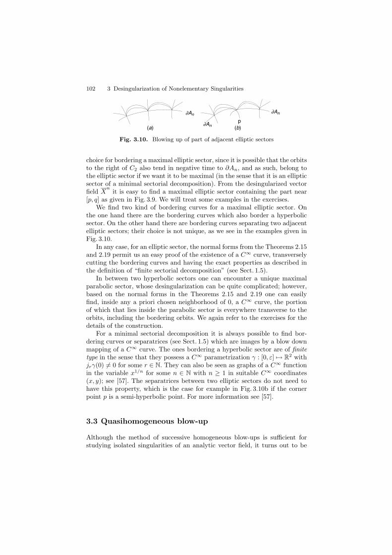
102 3 Desingularization of Nonelementary Singularities
(a)
p
∂An∂An
∂An(b)
Fig. 3.10. Blowing up of part of adjacent elliptic sectors
choice for bordering a maximal elliptic sector, since it is possible that the orbitsto the right of C2 also tend in negative time to ∂An, and as such, belong tothe elliptic sector if we want it to be maximal (in the sense that it is an ellipticsector of a minimal sectorial decomposition). From the desingularized vectorfield X
nit is easy to find a maximal elliptic sector containing the part near
[p, q] as given in Fig. 3.9. We will treat some examples in the exercises.We find two kind of bordering curves for a maximal elliptic sector. On
the one hand there are the bordering curves which also border a hyperbolicsector. On the other hand there are bordering curves separating two adjacentelliptic sectors; their choice is not unique, as we see in the examples given inFig. 3.10.
In any case, for an elliptic sector, the normal forms from the Theorems 2.15and 2.19 permit us an easy proof of the existence of a C∞ curve, transverselycutting the bordering curves and having the exact properties as described inthe definition of “finite sectorial decomposition” (see Sect. 1.5).
In between two hyperbolic sectors one can encounter a unique maximalparabolic sector, whose desingularization can be quite complicated; however,based on the normal forms in the Theorems 2.15 and 2.19 one can easilyfind, inside any a priori chosen neighborhood of 0, a C∞ curve, the portionof which that lies inside the parabolic sector is everywhere transverse to theorbits, including the bordering orbits. We again refer to the exercises for thedetails of the construction.
For a minimal sectorial decomposition it is always possible to find bor-dering curves or separatrices (see Sect. 1.5) which are images by a blow downmapping of a C∞ curve. The ones bordering a hyperbolic sector are of finitetype in the sense that they possess a C∞ parametrization γ : [0, ε] �→ R2 withjrγ(0) �= 0 for some r ∈ N. They can also be seen as graphs of a C∞ functionin the variable x1/n for some n ∈ N with n ≥ 1 in suitable C∞ coordinates(x, y); see [57]. The separatrices between two elliptic sectors do not need tohave this property, which is the case for example in Fig. 3.10b if the cornerpoint p is a semi-hyperbolic point. For more information see [57].
3.3 Quasihomogeneous blow-up
Although the method of successive homogeneous blow-ups is sufficient forstudying isolated singularities of an analytic vector field, it turns out to be
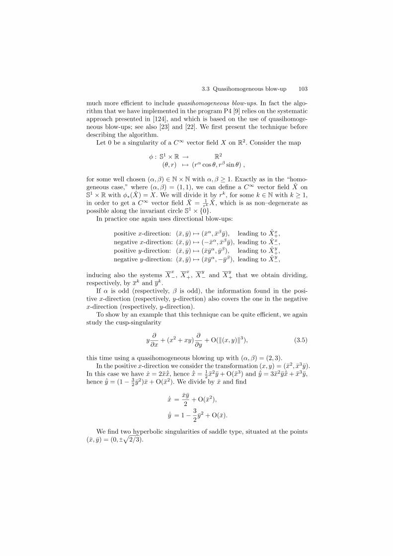
3.3 Quasihomogeneous blow-up 103
much more efficient to include quasihomogeneous blow-ups. In fact the algo-rithm that we have implemented in the program P4 [9] relies on the systematicapproach presented in [124], and which is based on the use of quasihomoge-neous blow-ups; see also [23] and [22]. We first present the technique beforedescribing the algorithm.
Let 0 be a singularity of a C∞ vector field X on R2. Consider the map
φ : S1 × R → R2
(θ, r) �→ (rα cos θ, rβ sin θ) ,
for some well chosen (α, β) ∈ N × N with α, β ≥ 1. Exactly as in the “homo-geneous case,” where (α, β) = (1, 1), we can define a C∞ vector field X onS1 × R with φ∗(X) = X. We will divide it by rk, for some k ∈ N with k ≥ 1,in order to get a C∞ vector field X = 1
rk X, which is as non–degenerate aspossible along the invariant circle S1 × {0}.
In practice one again uses directional blow-ups:
positive x-direction: (x, y) �→ (xα, xβ y), leading to Xx+,
negative x-direction: (x, y) �→ (−xα, xβ y), leading to Xx−,
positive y-direction: (x, y) �→ (xyα, yβ), leading to Xy+,
negative y-direction: (x, y) �→ (xyα,−yβ), leading to Xy−,
inducing also the systems Xx
−, Xx
+, Xy
− and Xy
+ that we obtain dividing,respectively, by xk and yk.
If α is odd (respectively, β is odd), the information found in the posi-tive x-direction (respectively, y-direction) also covers the one in the negativex-direction (respectively, y-direction).
To show by an example that this technique can be quite efficient, we againstudy the cusp-singularity
y∂
∂x+ (x2 + xy)
∂
∂y+ O(‖(x, y)‖3), (3.5)
this time using a quasihomogeneous blowing up with (α, β) = (2, 3).In the positive x-direction we consider the transformation (x, y) = (x2, x3y).
In this case we have x = 2x ˙x, hence ˙x = 12 x2y + O(x3) and ˙y = 3x2y ˙x + x3y,
hence ˙y = (1 − 32 y2)x + O(x2). We divide by x and find
˙x =xy
2+ O(x2),
˙y = 1 − 3
2y2 + O(x).
We find two hyperbolic singularities of saddle type, situated at the points(x, y) = (0,
√2/3).

104 3 Desingularization of Nonelementary Singularities
Fig. 3.11. Quasihomogeneous blow-up of the cusp singularity
Similar calculations in the negative x-direction, as well as in the y-directionshow that no other singularities are present.
As such blowing up once suffices to desingularize the singularity leadingto the picture in Fig. 3.11.
Again an accurate positioning of the invariant separatrices can be obtainedby Taylor approximation of the stable and unstable manifolds.
A question one might ask is how to effectively find the coefficient (α, β)to use in a quasihomogeneous blow-up. This can be obtained by using the socalled Newton diagram. We first define the Newton diagram.
Let X = P (x, y) ∂∂x + Q(x, y) ∂
∂y be a polynomial vector field with an iso-lated singularity at the origin.
Let P (x, y) =∑
i+j≥1
aijxiyj and Q(x, y) =
∑
i+j≥1
bijxiyj . The support of X
is defined to be
S = {(i − 1, j) : aij �= 0} ∪ {(i, j − 1) : bij �= 0} ⊂ R2,
and the Newton polygon of X is the convex hull Γ of the set
P =⋃
(r,s)∈S
{(r′, s′) : r′ ≥ r, s′ ≥ s}.
The Newton diagram of X is the union γ of the compact faces γk of theNewton polygon Γ, which we enumerate from the left to the right. If thereexists a face γk which lies completely on the half-plane {r ≤ 0}, then we startthe enumeration with k = 0, otherwise we start with k = 1. Since the originis an isolated singularity we have that at least one of the points (−1, s) or(0, s) is an element of S for some s, and also at least one of the points (r, 0)or (r,−1) is an element of S for some r. Hence there always exists a face γ1
in the Newton diagram.Suppose that γ1 has equation αr + βs = d, with gcd(α, β) = 1. As a first
step in the desingularization process we use a quasihomogeneous blow-up ofdegree (α, β). As an example we calculate the Newton diagram of the vectorfield (3.5), providing the best choice of coefficients (α, β).
The support of (3.5) surely contains (−1, 1), (2,−1), and (1, 0) coming,respectively, from y ∂
∂x , x2 ∂∂y , and xy ∂
∂y . Besides these three points it cancontain many other points, which are in fact not essential since they all lie
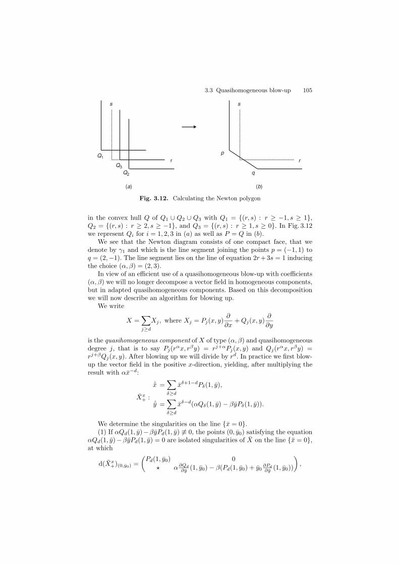
3.3 Quasihomogeneous blow-up 105
r r
s s
(a) (b)
Q1
Q2
Q3
p
q
Fig. 3.12. Calculating the Newton polygon
in the convex hull Q of Q1 ∪ Q2 ∪ Q3 with Q1 = {(r, s) : r ≥ −1, s ≥ 1},Q2 = {(r, s) : r ≥ 2, s ≥ −1}, and Q3 = {(r, s) : r ≥ 1, s ≥ 0}. In Fig. 3.12we represent Qi for i = 1, 2, 3 in (a) as well as P = Q in (b).
We see that the Newton diagram consists of one compact face, that wedenote by γ1 and which is the line segment joining the points p = (−1, 1) toq = (2,−1). The line segment lies on the line of equation 2r+3s = 1 inducingthe choice (α, β) = (2, 3).
In view of an efficient use of a quasihomogeneous blow-up with coefficients(α, β) we will no longer decompose a vector field in homogeneous components,but in adapted quasihomogeneous components. Based on this decompositionwe will now describe an algorithm for blowing up.
We write
X =∑
j≥d
Xj , where Xj = Pj(x, y)∂
∂x+ Qj(x, y)
∂
∂y
is the quasihomogeneous component of X of type (α, β) and quasihomogeneousdegree j, that is to say Pj(r
αx, rβy) = rj+αPj(x, y) and Qj(rαx, rβy) =
rj+βQj(x, y). After blowing up we will divide by rd. In practice we first blow-up the vector field in the positive x-direction, yielding, after multiplying theresult with αx−d:
Xx+ :
˙x =∑
δ≥d
xδ+1−dPδ(1, y),
˙y =∑
δ≥d
xδ−d(αQδ(1, y) − βyPδ(1, y)).
We determine the singularities on the line {x = 0}.(1) If αQd(1, y)−βyPd(1, y) �≡ 0, the points (0, y0) satisfying the equation
αQd(1, y)−βyPd(1, y) = 0 are isolated singularities of X on the line {x = 0},at which
d(Xx+)(0,y0) =
(Pd(1, y0) 0
⋆ α∂Qd
∂y (1, y0) − β(Pd(1, y0) + y0∂Pd
∂y (1, y0))
),
106 3 Desingularization of Nonelementary Singularities
which immediately gives the eigenvalues as the diagonal entries. If the sin-gularity is hyperbolic, we are done. If the singularity is semi-hyperbolic, wehave to determine the behavior on the center manifold. If the singularity isnonelementary, we introduce y = y − y0, and blow-up this vector field againin the positive x-direction as well as in the positive and negative y-directionwith a certain degree (α′, β′), which we determine from the Newton diagramassociated to the vector field.
(2) If αQd(1, y) − βyPd(1, y) ≡ 0, we have a line of singularities. Since
D(Xx+)(0,y0) =
(Pd(1, y0) 0
⋆ 0
),
all the singularities are semi-hyperbolic, except those singularities (0, y0) forwhich Pd(1, y0) = 0. The latter will require further blow-up.
Next we blow-up the vector field in the negative x-direction and study thisvector field in the same way as in the previous case.
Finally we have to blow-up the vector field in the positive and the negativey-direction, and determine whether or not (0, 0) is a singular point, since theothers have been studied in the previous charts.
It is easy to see that (0, 0) is a singularity if and only if γ1 lies completelyin the half-plane {r ≥ 0}. If this is the case then (0, 0) is elementary. Indeed,blowing up the vector field in the positive y-direction yields, after multiplyingthe result by βy−d:
Xy+ :
˙x =∑
δ≥d
yδ−d(βPδ(x, 1) − αxQδ(x, 1)),
˙y =∑
δ≥d
yδ+1−dQδ(x, 1).
Hence (0, 0) is a singular point if Pd(0, 1) = 0, i.e., if Pd(x, y) = xF (x, y),implying that γ1 lies completely in the half-plane {r ≥ 0}. Suppose now that(0, 0) is a singular point of Xy
+; then we have
D(Xy+)(0,0) =
(β ∂Pd
∂x (0, 1) − αQd(0, 1) ⋆0 Qd(0, 1)
).
Let (0, s) be the intersection of the line γ1 and the line r = 0. ThenPd(x, y) = axys + G(x, y) and Qd(x, y) = bys+1 + H(x, y), with a2 + b2 �=0, degx G(x, y) ≥ 2 and degx H(x, y) ≥ 1. Hence β ∂Pd
∂x (0, 1) − αQd(0, 1) =aβ − bα. So if aβ − bα �= 0 then (0, 0) is nonelementary. If aβ − bα = 0, thenQd(0, 1) = b �= 0, and (0, 0) is elementary, too.
In [124] it has been proven that the algorithm, as presented here, leads toa desingularization. It is also more efficient than the usual one.
In the program P4 [9] we not only perform a detailed study near thesingular points in R2, but also near singular points at infinity. In Chap. 5 wewill describe how polynomial vector fields on R2 can be extended to infinity.We now apply the blow-up technique to study nilpotent singularities.
3.4 Nilpotent Singularities 107
3.4 Nilpotent Singularities
In this section we study singularities, positioned at the origin, at which the
linear approximation DX(0) of the vector field X is linearly conjugate to y∂
∂x.
As usual we take X to be at least of class C∞; we recall that such asingularity is called a nilpotent singularity or nilpotent singular point.
Using the Formal Normal Form Theorem presented in Sect. 2.1 and, morespecifically, the example treated there, we find the following normal form forC∞-conjugacy:
x = y + A(x, y),
y = f(x) + yg(x) + y2B(x, y),
where f , g, A, and B are C∞ functions, j1f(0) = g(0) = j∞A(0, 0) =j∞B(0, 0) = 0. By introducing the new variable Y = y + A(x, y), we changethe former expression into
x = y,
y = f(x) + yg(x) + y2B(x, y),(3.6)
for appropriately adapted f , g, and B with similar properties as before. IfB ≡ 0, then the system comes from the Lienard equation x = f(x) + xg(x).We now make a complete local topological study of all cases in which j∞f(0)is not zero. This includes the local study of the related Lienard equations.Either j∞g(0) �= 0 and
f(x) = axm + o(xm),
g(x) = bxn + o(xn),(3.7)
with ab �= 0, or j∞g(0) = 0. The dual 1-form of (3.6) is given by
−ydy + (f(x) + yg(x) + y2B(x, y))dx,
which is equal to
− ydy + df(x) + ydg(x) + y2B(x, y)dx, (3.8)
for some C∞ functions f and g such that
f(x) =axm+1
m + 1+ o(xm+1) and
g(x) =bxn+1
n + 1+ o(xn+1),
provided j∞g(0) �= 0.A linear change in x permits f to be changed into
f(x) =δxm+1
m + 1+ o(xm+1),
108 3 Desingularization of Nonelementary Singularities
with δ = 1 in case m is even and δ = 1 in case m is odd. Changing y by −yif necessary we may suppose that b > 0. Instead of reducing a to δ, we couldalso perform on g an operation similar to the one performed on f to reduce bto +1, hence obtaining
g(x) =xn+1
n + 1+ o(xn+1),
provided j∞g(0) �= 0.So up to linear (not necessarily orientation preserving) equivalence, we can
suppose that in expression (3.7)
either a = δ and b > 0, or b = 1, (3.9)
with δ = 1 when m is even and δ = 1 when m is odd.If j∞g(0) �= 0, we observe that a coordinate change
y = Y +
∫ x
0
g(u)du = Y + G(x), (3.10)
permits changing an expression (3.6) with B ≡ 0 into
x = Y + G(x),
y = f(x).
If B �≡ 0, then (3.10) changes expression (3.6) into
x = Y + G(x),
Y = F (x) + Y H(x) + Y 2D(x, Y ),(3.11)
where G, F , H, and D are C∞ functions, j∞F (0) = j∞f(0), j∞H(0) =j∞D(0, 0) = 0. By a well chosen C∞ coordinate change Y = y + α(x) withj∞α(0) = 0 we can even change (3.11) into
x = y + G(x),
y = F (x) + y2C(x, y),(3.12)
with j∞G(0) = j∞G(0), j∞F (0) = j∞F (0) and j∞C(0, 0) = 0. Then expres-sion (3.12) is also valid if j∞g(0) = 0.
We write (3.12) asx = y + H(x),
y = F (x) + y2C(x, y),(3.13)
with H(0) = 0. The relation between (3.12) and (3.13) is given by
j∞H ′(0) = j∞g(0),
j∞F (0) = j∞f(0).

3.4 Nilpotent Singularities 109
The study of these singularities now relies on (quasihomogeneous) blow-up. We systematically work it out, depending on the values of m and n, wherem ≥ 2 and n ≥ 1 including n = ∞, the latter of which means that we acceptj∞g(0) = 0 in expression (3.6).
We distinguish three cases.Hamiltonian like case: m < 2n + 1. If m is odd we use the blow-up
x = u, y = uky, (3.14)
with k = (m + 1)/2 and we divide by uk−1.If m is even we use
x = u2, y = um+1y, (3.15)
and we divide by um−1.Singular like case: m > 2n + 1. We use the blow-up
x = u, y = un+1y, (3.16)
and we divide by un.Mixed case: m = 2n + 1. We use again the blow-up (3.16)
In all cases there is no need to check the directional charts {y = 1}because of the specific expression of the linear part. We may also restrict to{x = 1}, since the n-exponent in front of x is odd, except for blow-up (3.15).
3.4.1 Hamiltonian Like Case (m < 2n + 1)
We start with expression (3.8) for the dual 1-form and change f(x) toδxm+1/(m+1) by a coordinate change in x. This changes expression (3.6) byC∞ equivalence into
x = y,
y = δxm + y(bxn + o(xn)) + O(y2).
Case m odd: We know that δ = 1 and we use blow-up (3.14) in thex-direction (x, y) �−→ (u, uky), with k = (m + 1)/2. After division by uk−1
we getu = uy,
y = (δ − ky2) + O(u).
The blow-up and related phase portraits for this system that can be seen inFig. 3.13.
For δ = 1 we get a singularity of saddle-type. One can prove that it is C0-conjugate to a hyperbolic saddle, but we will not work it out, as announcedbefore. The contact between the different separatrices is described by theblowing up mapping.
For δ = −1 we get a singularity of center or focus type. It is not a simpleproblem to determine whether it is a center or a focus.
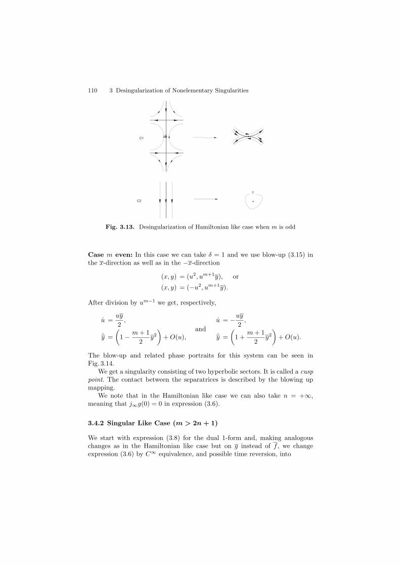
110 3 Desingularization of Nonelementary Singularities
C2
C1
?
Fig. 3.13. Desingularization of Hamiltonian like case when m is odd
Case m even: In this case we can take δ = 1 and we use blow-up (3.15) inthe x-direction as well as in the −x-direction
(x, y) = (u2, um+1y), or
(x, y) = (−u2, um+1y).
After division by um−1 we get, respectively,
u =uy
2,
y =
(1 − m + 1
2y2
)+ O(u),
and
u = −uy
2,
y =
(1 +
m + 1
2y2
)+ O(u).
The blow-up and related phase portraits for this system can be seen inFig. 3.14.
We get a singularity consisting of two hyperbolic sectors. It is called a cusppoint. The contact between the separatrices is described by the blowing upmapping.
We note that in the Hamiltonian like case we can also take n = +∞,meaning that j∞g(0) = 0 in expression (3.6).
3.4.2 Singular Like Case (m > 2n + 1)
We start with expression (3.8) for the dual 1-form and, making analogouschanges as in the Hamiltonian like case but on g instead of f , we changeexpression (3.6) by C∞ equivalence, and possible time reversion, into
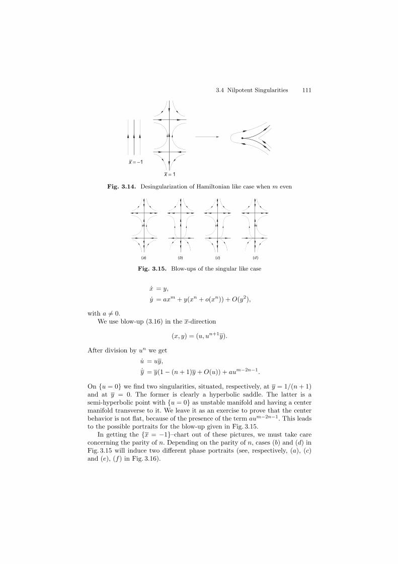
3.4 Nilpotent Singularities 111
x = −1−
x = 1−
Fig. 3.14. Desingularization of Hamiltonian like case when m even
(a) (b) (c) (d )
Fig. 3.15. Blow-ups of the singular like case
x = y,
y = axm + y(xn + o(xn)) + O(y2),
with a �= 0.We use blow-up (3.16) in the x-direction
(x, y) = (u, un+1y).
After division by un we get
u = uy,
y = y(1 − (n + 1)y + O(u)) + aum−2n−1.
On {u = 0} we find two singularities, situated, respectively, at y = 1/(n + 1)and at y = 0. The former is clearly a hyperbolic saddle. The latter is asemi-hyperbolic point with {u = 0} as unstable manifold and having a centermanifold transverse to it. We leave it as an exercise to prove that the centerbehavior is not flat, because of the presence of the term aum−2n−1. This leadsto the possible portraits for the blow-up given in Fig. 3.15.
In getting the {x = −1}–chart out of these pictures, we must take careconcerning the parity of n. Depending on the parity of n, cases (b) and (d) inFig. 3.15 will induce two different phase portraits (see, respectively, (a), (c)and (e), (f) in Fig. 3.16).
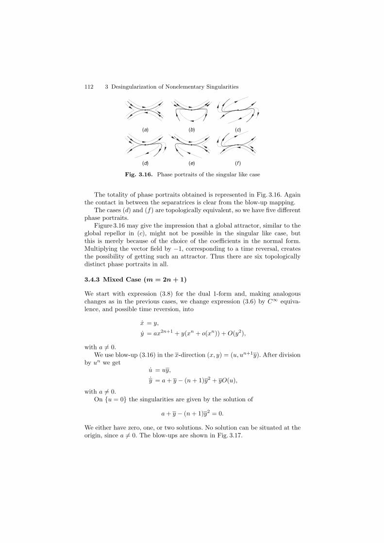
112 3 Desingularization of Nonelementary Singularities
(a)
(f )(d) (e)
(b) (c)
Fig. 3.16. Phase portraits of the singular like case
The totality of phase portraits obtained is represented in Fig. 3.16. Againthe contact in between the separatrices is clear from the blow-up mapping.
The cases (d) and (f) are topologically equivalent, so we have five differentphase portraits.
Figure 3.16 may give the impression that a global attractor, similar to theglobal repellor in (c), might not be possible in the singular like case, butthis is merely because of the choice of the coefficients in the normal form.Multiplying the vector field by −1, corresponding to a time reversal, createsthe possibility of getting such an attractor. Thus there are six topologicallydistinct phase portraits in all.
3.4.3 Mixed Case (m = 2n + 1)
We start with expression (3.8) for the dual 1-form and, making analogouschanges as in the previous cases, we change expression (3.6) by C∞ equiva-lence, and possible time reversion, into
x = y,
y = ax2n+1 + y(xn + o(xn)) + O(y2),
with a �= 0.We use blow-up (3.16) in the x-direction (x, y) = (u, un+1y). After division
by un we getu = uy,
y = a + y − (n + 1)y2 + yO(u),
with a �= 0.On {u = 0} the singularities are given by the solution of
a + y − (n + 1)y2 = 0.
We either have zero, one, or two solutions. No solution can be situated at theorigin, since a �= 0. The blow-ups are shown in Fig. 3.17.
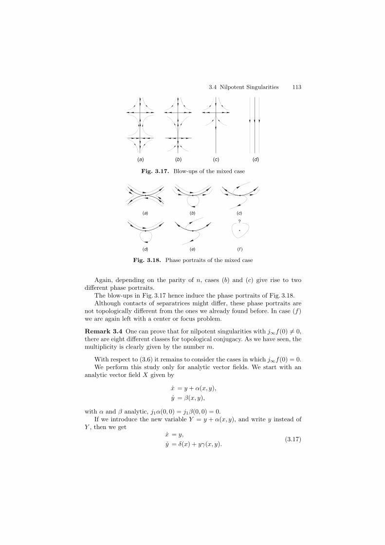
3.4 Nilpotent Singularities 113
(a) (b) (c) (d)
Fig. 3.17. Blow-ups of the mixed case
(a)
(f )(d) (e)
(b) (c)
?
Fig. 3.18. Phase portraits of the mixed case
Again, depending on the parity of n, cases (b) and (c) give rise to twodifferent phase portraits.
The blow-ups in Fig. 3.17 hence induce the phase portraits of Fig. 3.18.Although contacts of separatrices might differ, these phase portraits are
not topologically different from the ones we already found before. In case (f)we are again left with a center or focus problem.
Remark 3.4 One can prove that for nilpotent singularities with j∞f(0) �= 0,there are eight different classes for topological conjugacy. As we have seen, themultiplicity is clearly given by the number m.
With respect to (3.6) it remains to consider the cases in which j∞f(0) = 0.We perform this study only for analytic vector fields. We start with an
analytic vector field X given by
x = y + α(x, y),
y = β(x, y),
with α and β analytic, j1α(0, 0) = j1β(0, 0) = 0.If we introduce the new variable Y = y + α(x, y), and write y instead of
Y , then we getx = y,
y = δ(x) + yγ(x, y).(3.17)
114 3 Desingularization of Nonelementary Singularities
We now prove that
j∞f(0) = 0 if and only if δ(x) ≡ 0. (3.18)
The Normal Form Theorem relies on transformations of the form
(u, v) = (x + A(x, y), y + B(x, y)), (3.19)
with A and B polynomials of a given degree n; the procedure uses an inductionon n. To prove (3.18) we need only make a formal calculation, that is simplylook at ∞-jets at (0, 0). The operation to transform (3.17) to a normal formby means of (3.19) implies that
(1 +
∂A
∂x
)y +
∂A
∂y(δ(x) + yγ(x, y)) = y + B(x, y),
∂B
∂xy +
(1 +
∂B
∂y
)(δ(x) + yγ(x, y)) = f(x + A(x, y))
+ (y + B(x, y))Γ(x, y),
(3.20)
for some function Γ.If we consider the second equation at y = 0, this gives
(1 +
∂B
∂y(x, 0)
)δ(x) = f(x + A(x, 0)) + B(x, 0)Γ(x, 0).
Taking into account the degree of the terms, we see that jnδ(0) = jnf(0)when jn−1δ(0) = jn−1f(0) = 0.
An induction argument hence shows that both f and δ have the same termof lowest degree, with the same coefficient.
Therefore the condition j∞f(0) = 0 on the normal form implies thatδ(x) ≡ 0 in expression (3.17), and we get the vector field X given by
x = y,
y = yγ(x, y),(3.21)
for which {y = 0} is a line of singularities.We now prove that
j∞g(0) = 0 if and only if γ(x, 0) = 0. (3.22)
This means that, under the condition j∞f(0) = 0, j∞g(0) = 0 as well if andonly if the divergence of X is identically zero along the curve of singularities.
The proof of (3.22) is similar to the proof of (3.18). Instead of (3.20) wenow find the equations (at the ∞-jet level)
(1 +
∂A
∂x
)y +
∂A
∂yyγ(x, y) = y + B(x, y),
∂B
∂xy +
(1 +
∂B
∂y
)yγ(x, y) = (y + B(x, y))g(x + A(x, y)).
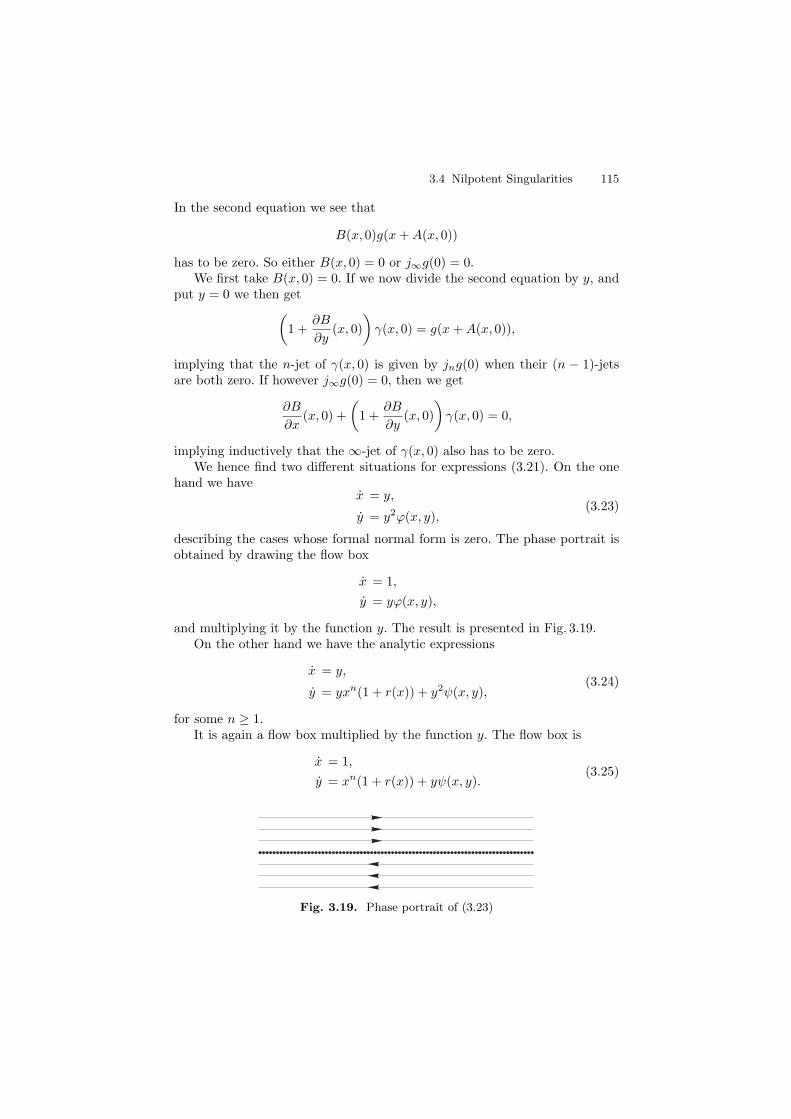
3.4 Nilpotent Singularities 115
In the second equation we see that
B(x, 0)g(x + A(x, 0))
has to be zero. So either B(x, 0) = 0 or j∞g(0) = 0.We first take B(x, 0) = 0. If we now divide the second equation by y, and
put y = 0 we then get(
1 +∂B
∂y(x, 0)
)γ(x, 0) = g(x + A(x, 0)),
implying that the n-jet of γ(x, 0) is given by jng(0) when their (n − 1)-jetsare both zero. If however j∞g(0) = 0, then we get
∂B
∂x(x, 0) +
(1 +
∂B
∂y(x, 0)
)γ(x, 0) = 0,
implying inductively that the ∞-jet of γ(x, 0) also has to be zero.We hence find two different situations for expressions (3.21). On the one
hand we havex = y,
y = y2ϕ(x, y),(3.23)
describing the cases whose formal normal form is zero. The phase portrait isobtained by drawing the flow box
x = 1,
y = yϕ(x, y),
and multiplying it by the function y. The result is presented in Fig. 3.19.On the other hand we have the analytic expressions
x = y,
y = yxn(1 + r(x)) + y2ψ(x, y),(3.24)
for some n ≥ 1.It is again a flow box multiplied by the function y. The flow box is
x = 1,
y = xn(1 + r(x)) + yψ(x, y).(3.25)
Fig. 3.19. Phase portrait of (3.23)
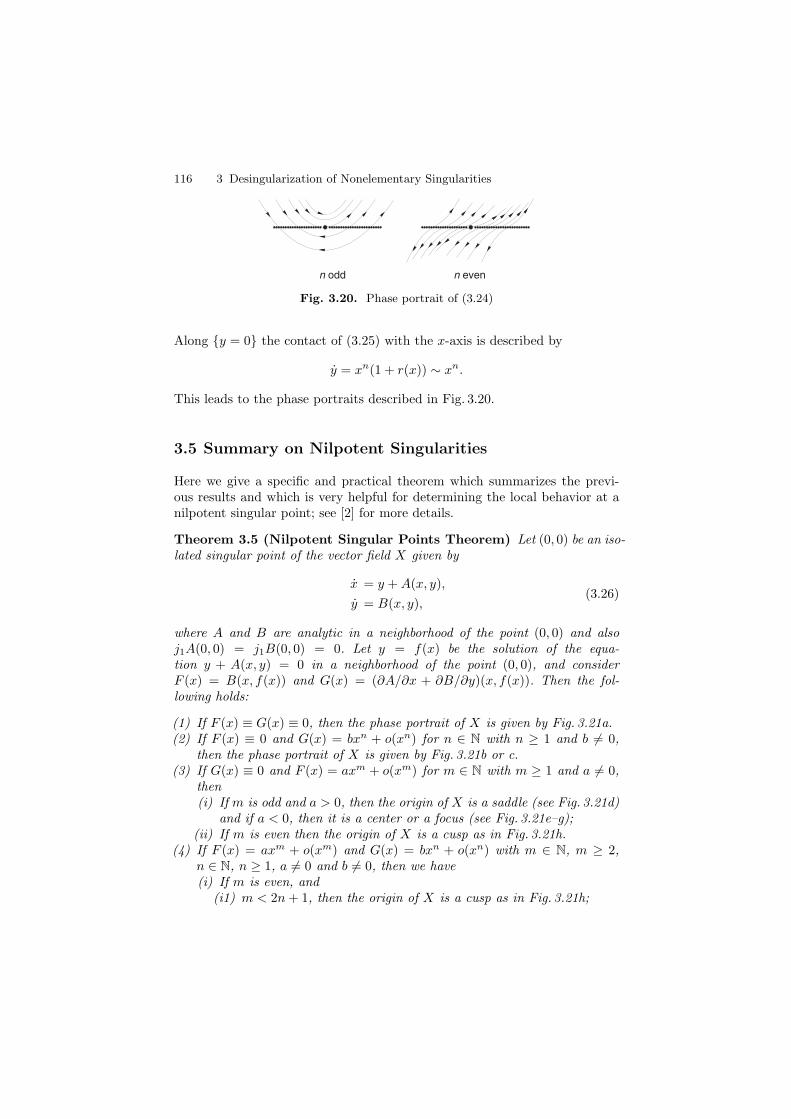
116 3 Desingularization of Nonelementary Singularities
n odd n even
Fig. 3.20. Phase portrait of (3.24)
Along {y = 0} the contact of (3.25) with the x-axis is described by
y = xn(1 + r(x)) ∼ xn.
This leads to the phase portraits described in Fig. 3.20.
3.5 Summary on Nilpotent Singularities
Here we give a specific and practical theorem which summarizes the previ-ous results and which is very helpful for determining the local behavior at anilpotent singular point; see [2] for more details.
Theorem 3.5 (Nilpotent Singular Points Theorem) Let (0, 0) be an iso-lated singular point of the vector field X given by
x = y + A(x, y),
y = B(x, y),(3.26)
where A and B are analytic in a neighborhood of the point (0, 0) and alsoj1A(0, 0) = j1B(0, 0) = 0. Let y = f(x) be the solution of the equa-tion y + A(x, y) = 0 in a neighborhood of the point (0, 0), and considerF (x) = B(x, f(x)) and G(x) = (∂A/∂x + ∂B/∂y)(x, f(x)). Then the fol-lowing holds:
(1) If F (x) ≡ G(x) ≡ 0, then the phase portrait of X is given by Fig. 3.21a.(2) If F (x) ≡ 0 and G(x) = bxn + o(xn) for n ∈ N with n ≥ 1 and b �= 0,
then the phase portrait of X is given by Fig. 3.21b or c.(3) If G(x) ≡ 0 and F (x) = axm + o(xm) for m ∈ N with m ≥ 1 and a �= 0,
then(i) If m is odd and a > 0, then the origin of X is a saddle (see Fig. 3.21d)
and if a < 0, then it is a center or a focus (see Fig. 3.21e–g);(ii) If m is even then the origin of X is a cusp as in Fig. 3.21h.
(4) If F (x) = axm + o(xm) and G(x) = bxn + o(xn) with m ∈ N, m ≥ 2,n ∈ N, n ≥ 1, a �= 0 and b �= 0, then we have(i) If m is even, and
(i1) m < 2n + 1, then the origin of X is a cusp as in Fig. 3.21h;
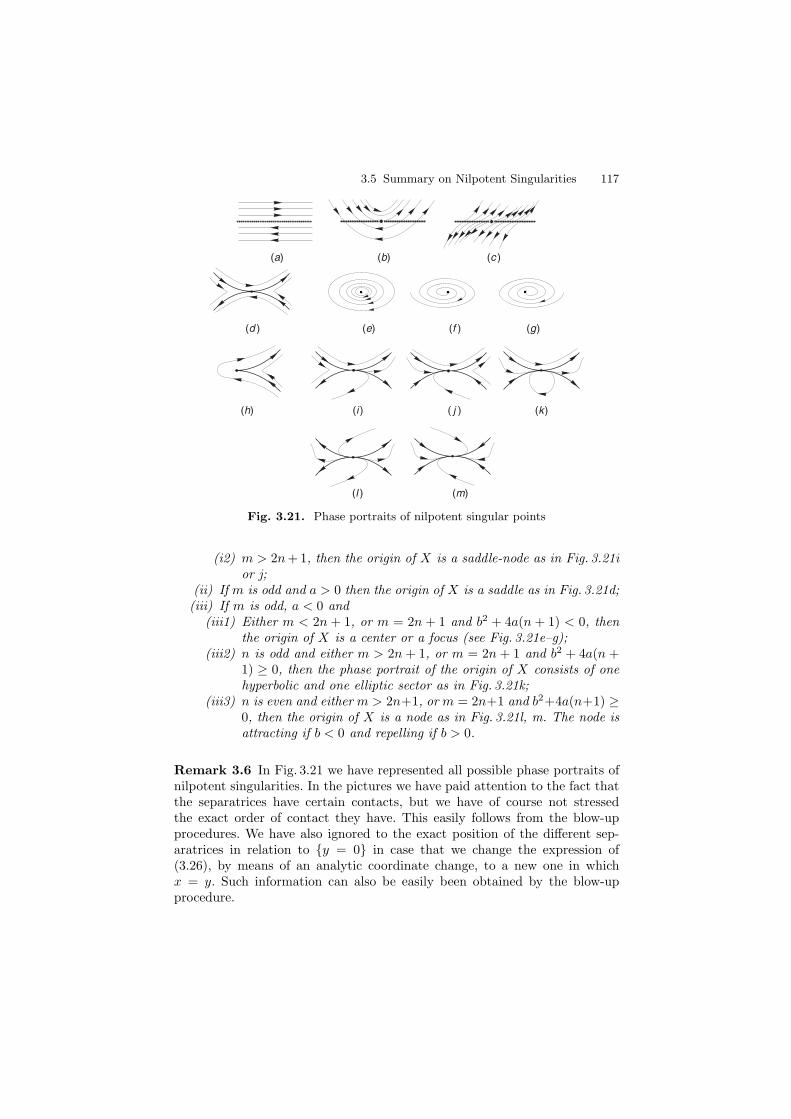
3.5 Summary on Nilpotent Singularities 117
(d )
(i ) (k)
(l )
(h)
(a)
(e)
(b) (c )
(g)(f )
( j )
(m)
Fig. 3.21. Phase portraits of nilpotent singular points
(i2) m > 2n + 1, then the origin of X is a saddle-node as in Fig. 3.21ior j;
(ii) If m is odd and a > 0 then the origin of X is a saddle as in Fig. 3.21d;(iii) If m is odd, a < 0 and
(iii1) Either m < 2n + 1, or m = 2n + 1 and b2 + 4a(n + 1) < 0, thenthe origin of X is a center or a focus (see Fig. 3.21e–g);
(iii2) n is odd and either m > 2n + 1, or m = 2n + 1 and b2 + 4a(n +1) ≥ 0, then the phase portrait of the origin of X consists of onehyperbolic and one elliptic sector as in Fig. 3.21k;
(iii3) n is even and either m > 2n+1, or m = 2n+1 and b2+4a(n+1) ≥0, then the origin of X is a node as in Fig. 3.21l, m. The node isattracting if b < 0 and repelling if b > 0.
Remark 3.6 In Fig. 3.21 we have represented all possible phase portraits ofnilpotent singularities. In the pictures we have paid attention to the fact thatthe separatrices have certain contacts, but we have of course not stressedthe exact order of contact they have. This easily follows from the blow-upprocedures. We have also ignored to the exact position of the different sep-aratrices in relation to {y = 0} in case that we change the expression of(3.26), by means of an analytic coordinate change, to a new one in whichx = y. Such information can also be easily been obtained by the blow-upprocedure.
118 3 Desingularization of Nonelementary Singularities
Remark 3.7 Section 3.4 has not really been arranged in such a way as tocontain a systematic proof of this theorem. We have preferred to treat thedifferent nilpotent singularities according to the kind of blow-up that is neededto study them. It is however clear that in order to get a precise proof ofTheorem 3.5 it is sufficient to go through the different cases and to apply theblow-ups as indicated in Sect. 3.4. We can leave this as an exercise.
The remaining center-focus problem, on the other hand, is an openproblem.
3.6 Exercises
Exercise 3.1 Consider the vector field (y +2x3) ∂∂x +(x2 +xy +y3) ∂
∂y . Makean appropriate quasihomogeneous blow-up at the origin and calculate a para-metrization γ : (R, 0) → (R2, 0) of the two separatrices, up to terms of order5, i.e., with a remainder of order O(t5).
Exercise 3.2 Study the following vector fields by means of an appropriatequasihomogeneous blow-up
(i) −y ∂∂x + x3 ∂
∂y ,
(ii) (y3 + xy2) ∂∂x + x2 ∂
∂y .
Exercise 3.3 Let X be a C∞ vector field satisfying a �Lojasiewicz inequalityat p and suppose that the C∞ vector field Y at q is C∞-conjugate to X at p.Show that Y at q also satisfies a �Lojasiewicz inequality.
Exercise 3.4 Check that the following vector fields satisfy a �Lojasiewiczinequality at the origin:
(i) (y + x3) ∂∂x − x3 ∂
∂y .
(ii) (x + y) ∂∂x + y4 ∂
∂y .
Exercise 3.5 Prove that a �Lojasiewicz inequality holds for
(i) all hyperbolic singularities.(ii) Singularities whose 1-jet is a center.(iii) Semi-hyperbolic singularities with nonflat center behavior.(iv) Nilpotent singularities for which in (3.6) j∞f(0) �= 0 holds.
Exercise 3.6 Prove that a C∞ vector field X satisfies a �Lojasiewicz inequal-ity at a singularity p if and only if there exists a finite jet jkX(p) with theproperty that ||jkX(p)|| ≥ c||x||k for some c > 0.
Exercise 3.7 Prove that no �Lojasiewicz inequality holds for the vector field
X = (y + x2)2∂
∂x+ (y + x2)
∂
∂y,

3.6 Exercises 119
but its 2-jet j2X(0) does satisfy a �Lojasiewicz inequality ||j2X(0)|| ≥ c||x||4for some c > 0.
Exercise 3.8 Prove the existence of a finite sectorial decomposition for thefollowing singularities at (0, 0).
(i) y ∂∂x + x2 ∂
∂y ,
(ii) (3x2 − 2xy) ∂∂x + (y2 − 3xy) ∂
∂y ,
(iii) (x2 − y2) ∂∂x + 2xy ∂
∂y ,
(iv) x2 ∂∂x + y(2x − y) ∂
∂y
Exercise 3.9 Consider the vector field in Example 3.1, of which the localphase portrait is represented in Fig. 3.2,
X = (x2 − 2xy)∂
∂x+ (y2 − xy)
∂
∂y+ O(‖(x, y‖3).
(i) Show that for ε sufficiently small, the six separatrices of this system cutSε = {(x, y)|x2 + y2 = ε} transversely.
(ii) Show that for each of these systems the “finite sectorial decomposition”property holds on some neighborhood V of the origin.
(iii) Prove that any two of the above systems are locally C0-equivalent.(iv) Show that inside any hyperbolic sector, the time to go from the boundary
∂V to itself tends monotonically to infinity when the orbit approaches theseparatrices.
(v) Use (iv) to prove that any two of the above systems are mutually C0-conjugate.
Exercise 3.10 Show that for any C∞ singularity of �Lojasiewicz type (sat-isfying a �Lojasiewicz inequality) with a characteristic orbit, there is a finitesectorial decomposition whose boundary is C∞.
Remark: The proof of the existence of a C∞ boundary relies on the use ofa “C∞-partition of the unity.” As a first step in the proof we suggest provingthe existence of a C0 boundary.
Exercise 3.11 Check that every C∞ singularity that satisfies a �Lojasiewiczinequality but does not have a characteristic orbit is necessarily monodromic.
Hint: Provide a proof based on the theorems that are cited in the book,even those whose proof is not incorporated.
Exercise 3.12 Use Theorem 3.5 to check the nature of the singularity at theorigin of
(−x2 + ay2 − xy − 2xy2)∂
∂x+ (y2 + xy + y3)
∂
∂y,
with a �= 0 and 1 + 2a > 0.
120 3 Desingularization of Nonelementary Singularities
3.7 Bibliographical Comments
The desingularization theorem for planar vector fields has a long history. Itwas first stated by Bendixson in 1901, however without proof. The paper alsoincluded the topological classification of the elementary singular points.
In 1968, Seidenberg gave the first rigorous proof of the theorem for theanalytic case. The desingularization procedure was extended to C∞ vectorfields of �Lojasiewicz type in [52]. This paper is based on the Ph.D.–thesis ofDumortier from 1973. In the mid seventies, van den Essen found a transformedproof of the desingularization theorem for analytic vector fields; see [159].
In all previous papers, the desingularization was based on quadratic trans-formations, or in the real case, on polar blow-up, hence in the terminology ofthis chapter, on the homogeneous blow-up.
Quasihomogeneous blow-up was already used in the book of Lyapunov[106] but was essentially put forward as a systematic and a more powerfultechnique in the paper by Brunella and Miari [22] and especially in the bookof Bruno [23]. A proof of the desingularization theorem for C∞ vector fields of�Lojasiewicz type, based on quasihomogeneous blow-ups, was given by Pelletierin her thesis [124]; see also [125]. The desingularization procedure used inthe program P4 [9] is based on the algorithm presented in that thesis. Theclassification of nilpotent singularities can be found in the papers of Andreev[2] and of Arrowsmith [8]. The elaboration that we provide in this chapteris based on quasihomogeneous blow-up and is by far the simplest that seemspossible.

4
Centers and Lyapunov Constants
One of the more classical problems in the qualitative theory of planar differ-ential equations is the problem of distinguishing between a focus and a center.This problem is unsolved in general, but in the case that the singular point is alinear center there are algorithms for solving it. The present chapter providesone of the best of these algorithms.
4.1 Introduction
Suppose that P and Q are analytic functions defined in a neighborhood of theorigin, and that (x, y) = (0, 0) is a singular point, linearly a focus or a center,for the system
x = P (x, y), y = Q(x, y).
Doing a suitable linear change of variables, the system can written in theform
x = λx + y + p(x, y), y = −x + λy + q(x, y), (4.1)
where p and q are analytic functions without constant or linear terms. If λ �= 0the origin is a strong focus, stable if λ < 0, and unstable if λ > 0. If λ = 0the origin is either a weak focus or a center. The search for necessary andsufficient conditions on p and q for the origin to be a center has a long historyand many methods have been developed. When the origin is a center thereexists an analytic first integral; this result is due to Poincare and for a proofsee [90].
Recently, the problem of distinguishing between a weak focus and a centerhas been stimulated considerably by the use of computer algebra systems. Inparticular, it has been made possible to find necessary and sufficient conditionsfor a singularity to be a center for many classes of systems of the form (4.1)which had previously been intractable.
In this chapter we will provide an algorithm for distinguishing betweena focus and a center when the system is linearly a center, that is, when the
122 4 Centers and Lyapunov Constants
eigenvalues at the origin are purely imaginary. In the first section of thischapter we present the normal form for singularities having a linear center.The rest of the chapter is dedicated to the algorithm and to its applications.
4.2 Normal Form for Linear Centers
In this section we will follow the notations and definitions introduced inSect. 2.1.
We calculate the normal forms for singularities having a linear center.Although it is not necessary, we use complex coordinates, since it simplifiesthe calculations.
Take z = x + iy and z = x − iy; as we know
∂
∂z=
1
2
(∂
∂x− i
∂
∂y
),
∂
∂z=
1
2
(∂
∂x+ i
∂
∂y
)
and
α
(x
∂
∂y− y
∂
∂x
)= iα
(z
∂
∂z− z
∂
∂z
),
[z
∂
∂z− z
∂
∂z, zizj ∂
∂z
]= (i − 1 − j)zizj ∂
∂z,
[z
∂
∂z− z
∂
∂z, zizj ∂
∂z
]= (i + 1 − j)zizj ∂
∂z.
We have that Ker ad2mA = {0}, while the kernel of ad2m+1A is spanned by{(zz)mz
∂
∂z, (zz)mz
∂
∂z
}, or by
{(zz)mi
(z
∂
∂z− z
∂
∂z
), (zz)m
(z
∂
∂z+ z
∂
∂z
)}=
{(x2 + y2)m
(x
∂
∂y− y
∂
∂x
), (x2 + y2)m
(x
∂
∂x+ y
∂
∂y
)}.
This leads to the ∞-jet
(α + f(x2 + y2))
(x
∂
∂y− y
∂
∂x
)+ g(x2 + y2)
(x
∂
∂x+ y
∂
∂y
),
with f(0) = g(0) = 0, which is the normal form for C∞ conjugacy of a linearcenter. If we divide it by (α + f(x2 + y2)) we get the following normal formfor C∞ equivalence:
(x
∂
∂y− y
∂
∂x
)+ h(x2 + y2)
(x
∂
∂x+ y
∂
∂y
). (4.2)
Both normal forms are only formal and not C∞; it is in general not pos-sible to remove extra flat terms, as we did in Sect. 2.7 for the elementary
4.2 Normal Form for Linear Centers 123
singularities. The formal series f , g, and h are also not convergent in general,not even for analytic (4.1). Nevertheless we now show how to prove that ananalytic (4.1) represents a center if and only if h is identically zero.
We consider a planar analytic differential equation
x = −y + P (x, y) = −y +∞∑
k=2
Pk(x, y),
y = x + Q(x, y) = x +∞∑
k=2
Qk(x, y),
(4.3)
where Pk and Qk are homogeneous polynomials of degree k. We can also writeit in polar coordinates (r, θ):
dr
dθ=
∞∑
k=2
Sk(θ)rk, (4.4)
where Sk(θ) are trigonometric polynomials in the variables sin(θ) and cos(θ);or in complex coordinates (z, z):
z = iz +∞∑
k=2
Rk(z, z), (4.5)
where Rk are homogeneous polynomials of degree k in z, z.If we denote by r(θ, r0) the solution of (4.4) such that r(0, r0) = r0 then
close to r = 0 we have
r(θ, r0) = r0 +∞∑
k=2
uk(θ)rk0 ,
with uk(0) = 0 for k ≥ 2. The Poincare return map near r = 0 is expressedby
Π(r0) = r(2π, r0) = r0 +
∞∑
k=2
uk(2π)rk0 .
Since Π is analytic it is clear that Π(r0) ≡ r0, and hence that (4.3) rep-resents a center, if and only if un(2π) = 0 for all n. Suppose for a momentthat this is not the case and let K be the smallest natural number such thatuK(2π) �= 0. This K clearly does not depend on the analytic coordinates cho-sen, nor does it change when we multiply the vector field by a positive analyticfunction. We can hence use the fact that (4.3) is analytically equivalent to ananalytic equation whose (2k + 1)-jet is given by
(x
∂
∂y− y
∂
∂x
)+
k∑
l=1
al(x2 + y2)l
(x
∂
∂x+ y
∂
∂y
), (4.6)
with k = [K/2].
124 4 Centers and Lyapunov Constants
The analytic equation can be written in polar coordinates as
dr
dθ=
k∑
l=1
alr2l + O(r2k+2). (4.7)
It is a straightforward calculation to show that necessarily a1 = . . . =ak−1 = 0, that K = 2k + 1, hence is odd, and that
uK(2π) = 2πak. (4.8)
Our claim follows from relation (4.8), which also gives a nice relation be-tween the first nonzero term of h and the first nonzero term of Π−Id.
When P and Q are polynomials, by the Hilbert Basis Theorem, there existsa m ∈ N with m ≥ 1 such that h = 0 if and only if jmh(0) = 0.
Although (4.2) is quite simple, it turns out that in many applications thecurrent status of computer technology does not permit its calculation, to therequired order, within a reasonable amount of time. The formulas also becomerather intractable if many parameters are involved. We therefore will now payattention to different techniques.
4.3 The Main Result
In several papers starting with Poincare and Lyapunov it has been shownhow necessary conditions are obtained by calculating the “focal values.” Itis well known (see e.g., [106]) that there exists a formal series V (x, y) =(x2 + y2)/2 + O(‖(x, y)‖3) such that V (its rate of change along orbits) is ofthe form
V = η2r2 + η4r
4 + . . . + η2kr2k + . . . ,
where r2 = x2 +y2. The η2k are called the focal values and are polynomials inthe coefficients of p and q. We will not prove this, since we will merely workwith the first nonzero term. So we prove the existence and uniqueness of someη2l for which there exists V (x, y) = (x2 + y2)/2 + O(‖(x, y)‖3) with
V = η2lr2l + O(r2l+1).
Such an expression, including the value of η2l, is invariant under near-identity transformations as well as under multiplication of the vector fieldwith a function f , that has the property f(0) = 1. We can hence suppose that(4.3) has the form
(x
∂
∂y− y
∂
∂x
)+ ak(x2 + y2)k
(x
∂
∂x+ y
∂
∂y
)+ Y, (4.9)
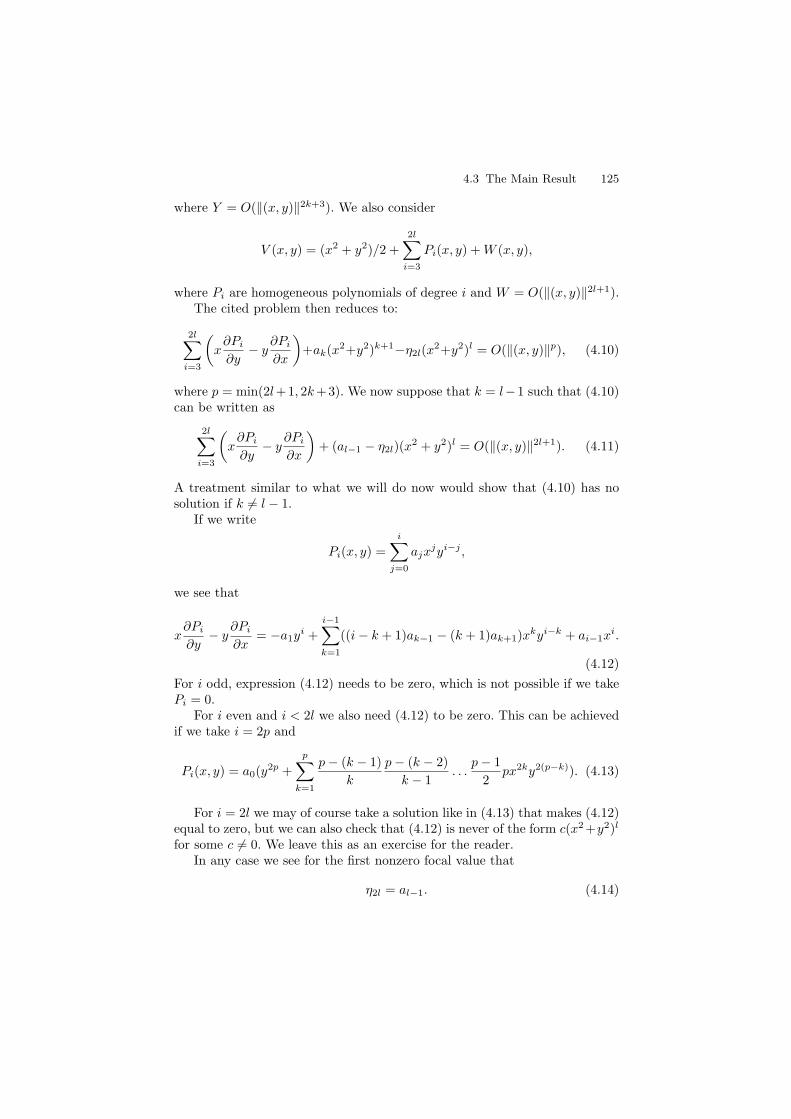
4.3 The Main Result 125
where Y = O(‖(x, y)‖2k+3). We also consider
V (x, y) = (x2 + y2)/2 +
2l∑
i=3
Pi(x, y) + W (x, y),
where Pi are homogeneous polynomials of degree i and W = O(‖(x, y)‖2l+1).The cited problem then reduces to:
2l∑
i=3
(x
∂Pi
∂y− y
∂Pi
∂x
)+ak(x2+y2)k+1−η2l(x
2+y2)l = O(‖(x, y)‖p), (4.10)
where p = min(2l+1, 2k +3). We now suppose that k = l−1 such that (4.10)can be written as
2l∑
i=3
(x
∂Pi
∂y− y
∂Pi
∂x
)+ (al−1 − η2l)(x
2 + y2)l = O(‖(x, y)‖2l+1). (4.11)
A treatment similar to what we will do now would show that (4.10) has nosolution if k �= l − 1.
If we write
Pi(x, y) =
i∑
j=0
ajxjyi−j ,
we see that
x∂Pi
∂y− y
∂Pi
∂x= −a1y
i +
i−1∑
k=1
((i − k + 1)ak−1 − (k + 1)ak+1)xkyi−k + ai−1x
i.
(4.12)
For i odd, expression (4.12) needs to be zero, which is not possible if we takePi = 0.
For i even and i < 2l we also need (4.12) to be zero. This can be achievedif we take i = 2p and
Pi(x, y) = a0(y2p +
p∑
k=1
p − (k − 1)
k
p − (k − 2)
k − 1. . .
p − 1
2px2ky2(p−k)). (4.13)
For i = 2l we may of course take a solution like in (4.13) that makes (4.12)equal to zero, but we can also check that (4.12) is never of the form c(x2+y2)l
for some c �= 0. We leave this as an exercise for the reader.In any case we see for the first nonzero focal value that
η2l = al−1. (4.14)
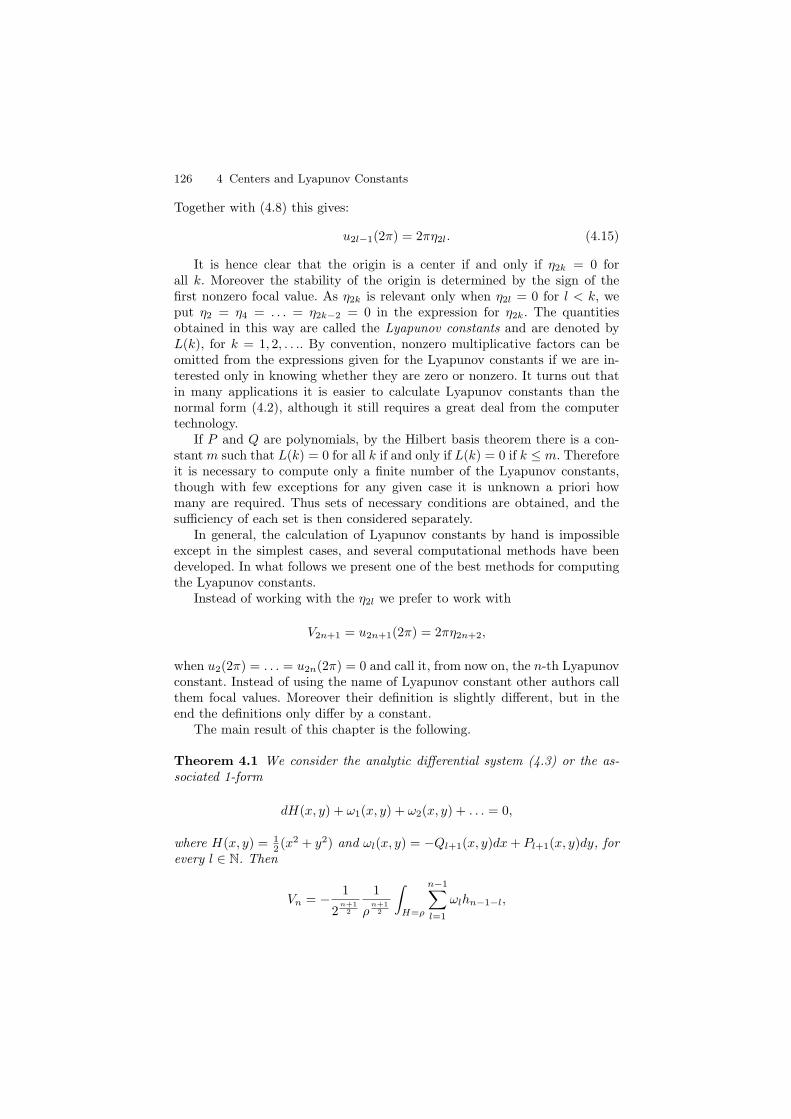
126 4 Centers and Lyapunov Constants
Together with (4.8) this gives:
u2l−1(2π) = 2πη2l. (4.15)
It is hence clear that the origin is a center if and only if η2k = 0 forall k. Moreover the stability of the origin is determined by the sign of thefirst nonzero focal value. As η2k is relevant only when η2l = 0 for l < k, weput η2 = η4 = . . . = η2k−2 = 0 in the expression for η2k. The quantitiesobtained in this way are called the Lyapunov constants and are denoted byL(k), for k = 1, 2, . . .. By convention, nonzero multiplicative factors can beomitted from the expressions given for the Lyapunov constants if we are in-terested only in knowing whether they are zero or nonzero. It turns out thatin many applications it is easier to calculate Lyapunov constants than thenormal form (4.2), although it still requires a great deal from the computertechnology.
If P and Q are polynomials, by the Hilbert basis theorem there is a con-stant m such that L(k) = 0 for all k if and only if L(k) = 0 if k ≤ m. Thereforeit is necessary to compute only a finite number of the Lyapunov constants,though with few exceptions for any given case it is unknown a priori howmany are required. Thus sets of necessary conditions are obtained, and thesufficiency of each set is then considered separately.
In general, the calculation of Lyapunov constants by hand is impossibleexcept in the simplest cases, and several computational methods have beendeveloped. In what follows we present one of the best methods for computingthe Lyapunov constants.
Instead of working with the η2l we prefer to work with
V2n+1 = u2n+1(2π) = 2πη2n+2,
when u2(2π) = . . . = u2n(2π) = 0 and call it, from now on, the n-th Lyapunovconstant. Instead of using the name of Lyapunov constant other authors callthem focal values. Moreover their definition is slightly different, but in theend the definitions only differ by a constant.
The main result of this chapter is the following.
Theorem 4.1 We consider the analytic differential system (4.3) or the as-sociated 1-form
dH(x, y) + ω1(x, y) + ω2(x, y) + . . . = 0,
where H(x, y) = 12 (x2 + y2) and ωl(x, y) = −Ql+1(x, y)dx + Pl+1(x, y)dy, for
every l ∈ N. Then
Vn = − 1
2n+1
2
1
ρn+1
2
∫
H=ρ
n−1∑
l=1
ωlhn−1−l,
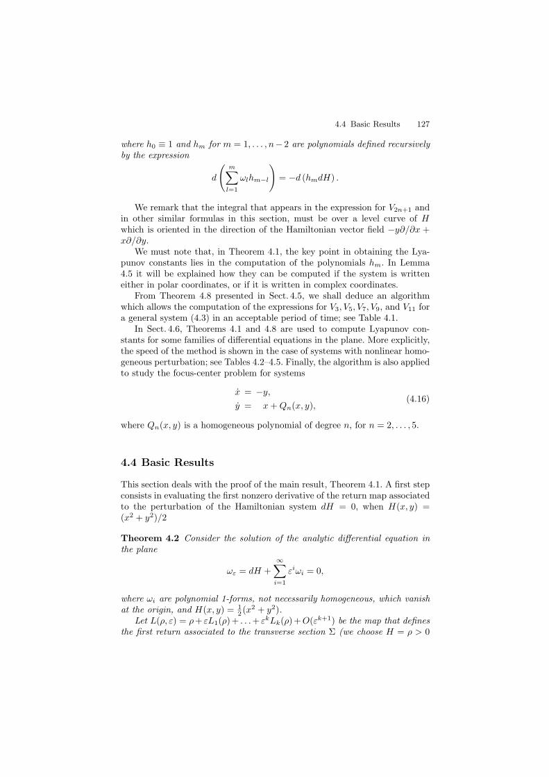
4.4 Basic Results 127
where h0 ≡ 1 and hm for m = 1, . . . , n− 2 are polynomials defined recursivelyby the expression
d
(m∑
l=1
ωlhm−l
)= −d (hmdH) .
We remark that the integral that appears in the expression for V2n+1 andin other similar formulas in this section, must be over a level curve of Hwhich is oriented in the direction of the Hamiltonian vector field −y∂/∂x +x∂/∂y.
We must note that, in Theorem 4.1, the key point in obtaining the Lya-punov constants lies in the computation of the polynomials hm. In Lemma4.5 it will be explained how they can be computed if the system is writteneither in polar coordinates, or if it is written in complex coordinates.
From Theorem 4.8 presented in Sect. 4.5, we shall deduce an algorithmwhich allows the computation of the expressions for V3, V5, V7, V9, and V11 fora general system (4.3) in an acceptable period of time; see Table 4.1.
In Sect. 4.6, Theorems 4.1 and 4.8 are used to compute Lyapunov con-stants for some families of differential equations in the plane. More explicitly,the speed of the method is shown in the case of systems with nonlinear homo-geneous perturbation; see Tables 4.2–4.5. Finally, the algorithm is also appliedto study the focus-center problem for systems
x = −y,
y = x + Qn(x, y),(4.16)
where Qn(x, y) is a homogeneous polynomial of degree n, for n = 2, . . . , 5.
4.4 Basic Results
This section deals with the proof of the main result, Theorem 4.1. A first stepconsists in evaluating the first nonzero derivative of the return map associatedto the perturbation of the Hamiltonian system dH = 0, when H(x, y) =(x2 + y2)/2
Theorem 4.2 Consider the solution of the analytic differential equation inthe plane
ωε = dH +∞∑
i=1
εiωi = 0,
where ωi are polynomial 1-forms, not necessarily homogeneous, which vanishat the origin, and H(x, y) = 1
2 (x2 + y2).Let L(ρ, ε) = ρ+ εL1(ρ)+ . . .+ εkLk(ρ)+O(εk+1) be the map that defines
the first return associated to the transverse section Σ (we choose H = ρ > 0

128 4 Centers and Lyapunov Constants
to parametrize the transverse section Σ). We assume that L1(ρ) ≡ . . . ≡Lm−1(ρ) ≡ 0. Then there exist polynomials h0 ≡ 1, h1, . . . , hm−1 such that
d
(m∑
i=1
ωihm−i
)= −d(hmdH),
and the mth derivative of L with respect to ε is m!Lm(ρ), with
Lm(ρ) = −∫
H=ρ
m∑
i=1
ωihm−i.
We must observe that the usefulness of these theorems in evaluating theLyapunov constants primarily depends on the way that one can calculatethe polynomials hj . In [65], the author chooses complex coordinates. In [157]the authors use both complex and polar coordinates. The results which followshow how the polynomials hj are found in these cases. The first is just areformulation of the results of [65], while the second will allow us to extendTheorem 4.1 to other Hamiltonian different from H = 1
2 (x2 + y2), like forinstance H = 1
4 (x4 + 2y2).We first introduce a bit of notation, and we also prove a technical lemma.
Lemma 4.3 Consider the 1-differential form ω = A(z, z)dz+B(z, z)dz, withA and B polynomials in z and z. Then
∫
H=ρ
ω = −2πi∑
k
coef
(− ∂
∂zA +
∂
∂zB, zkzk
)(2ρ)k+1
k + 1,
where the function coef(f, zkzl) gives the coefficient of the monomial zkzl, forevery k and l, of f .
Proof. From Stokes’ Theorem we have that
∫
H=ρ
ω =
∫
H=ρ
(A(z, z)dz + B(z, z)dz)
=
∫
H≤ρ
d (A(z, z)dz + B(z, z)dz)
=
∫
H≤ρ
(∂A
∂zdz ∧ dz +
∂B
∂zdz ∧ dz
)
=
∫
H≤ρ
(−∂A
∂z+
∂B
∂z
)dz ∧ dz.
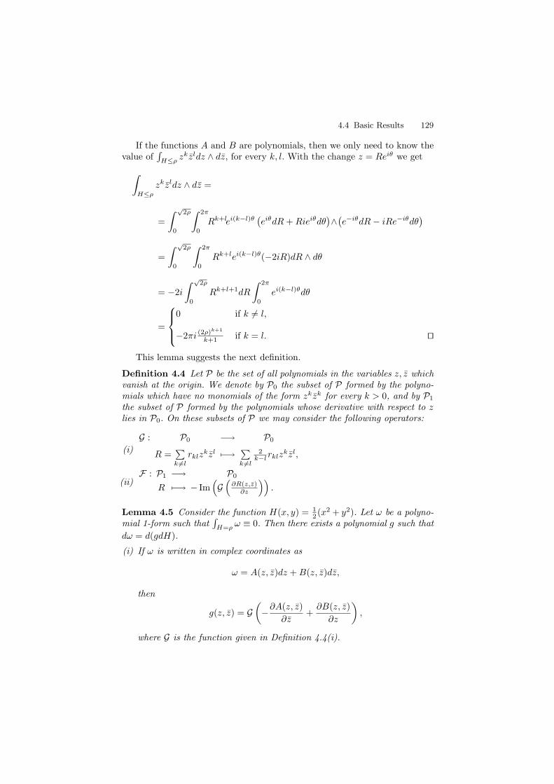
4.4 Basic Results 129
If the functions A and B are polynomials, then we only need to know thevalue of
∫H≤ρ
zkzldz ∧ dz, for every k, l. With the change z = Reiθ we get
∫
H≤ρ
zkzldz ∧ dz =
=
∫ √2ρ
0
∫ 2π
0
Rk+lei(k−l)θ(eiθdR + Rieiθdθ
)∧(e−iθdR − iRe−iθdθ
)
=
∫ √2ρ
0
∫ 2π
0
Rk+lei(k−l)θ(−2iR)dR ∧ dθ
= −2i
∫ √2ρ
0
Rk+l+1dR
∫ 2π
0
ei(k−l)θdθ
=
⎧⎪⎨⎪⎩
0 if k �= l,
−2πi (2ρ)k+1
k+1 if k = l. ⊓⊔
This lemma suggests the next definition.
Definition 4.4 Let P be the set of all polynomials in the variables z, z whichvanish at the origin. We denote by P0 the subset of P formed by the polyno-mials which have no monomials of the form zkzk for every k > 0, and by P1
the subset of P formed by the polynomials whose derivative with respect to zlies in P0. On these subsets of P we may consider the following operators:
(i)
G : P0 −→ P0
R =∑k =l
rklzkzl �−→ ∑
k =l
2k−lrklz
kzl,
(ii)F : P1 −→ P0
R �−→ − Im(G(
∂R(z,z)∂z
)).
Lemma 4.5 Consider the function H(x, y) = 12 (x2 + y2). Let ω be a polyno-
mial 1-form such that∫
H=ρω ≡ 0. Then there exists a polynomial g such that
dω = d(gdH).
(i) If ω is written in complex coordinates as
ω = A(z, z)dz + B(z, z)dz,
then
g(z, z) = G(−∂A(z, z)
∂z+
∂B(z, z)
∂z
),
where G is the function given in Definition 4.4(i).

130 4 Centers and Lyapunov Constants
(ii) If ω is written in polar coordinates as
ω = α(r, θ)dr + β(r, θ)dθ,
then
g(r, θ) =1
r
∫ θ
0
(∂α(r, ψ)
∂ψ− ∂β(r, ψ)
∂r
)dψ.
We must note that in the proof of item (i) of Lemma 4.5 we strongly usethe hypothesis
∫H=ρ
ω ≡ 0, in order to define the polynomial g. On the other
hand, the construction of g in item (ii) does not depend on the hypothesis∫H=ρ
ω ≡ 0. This hypothesis is needed only to assure that the g obtained is atrigonometric polynomial, using that g is 2π-periodic in θ.
From Lemma 4.5 we get that g satisfies dω = d (gdH). Thus we can saythat there exists a function S such that ω = gdH + dS.
Proof of Lemma 4.5. (i) It is clear from Lemma 4.3 that∫
H=ρω ≡ 0 if and
only if the polynomial − ∂∂z A+ ∂
∂z B has no monomial of the form (zz)k. So thepolynomial g(z, z) of the statement is well defined. If we define the polynomial
D(z, z) = − ∂
∂zA +
∂
∂zB =
∑
k =l
dklzkzl,
then
g(z, z)dH =
⎛⎝∑
k =l
2
k − ldklz
kzl
⎞⎠ 1
2(zdz + zdz) ,
where every monomial satisfies
d
((dkl
k − lzkzl
)(zdz + zdz)
)=
dkl
k − ld(zkzl+1dz + zk+1zldz
)
= dklzkzldz ∧ dz.
Therefore g(z, z) verifiesdω = d(g(z, z)dH),
because dω = D(z, z)dz ∧ dz.(ii) From the expressions of the function H = 1
2r2 and the 1-form ω =
αdr + βdθ, we obtain that dω = (−∂α∂θ + ∂β
∂r )dr ∧ dθ and d(g(r, θ)rdr) =
−r ∂g∂θ dr ∧ dθ which coincide in the case that the function g is defined as in
the statement. ⊓⊔
4.4 Basic Results 131
Proof of Lemma 4.2. Let γε be the solution curve of ωε = 0 defining L(ρ, ε);γ0 is the curve which defines H = ρ. So it is clear that over γε the 1-form ωε
vanishes, and we have ∫
γε
ωε = 0.
Integration over γε is taken in the same sense as for γ0. Substituting in thisequality the expression for ωε, we get
0 =
∫
γε
(dH + εω1 + ε2ω2 + . . .
)
= H(L(ρ, ε)) − H(ρ) + ε
∫
γε
ω1 + ε2
∫
γε
ω2 + . . .
=(ρ + L1(ρ)ε + L2(ρ)ε2 + . . .
)− ρ + ε
∫
γ0
(ω1 + O(ε))
+ ε2
∫
γ0
(ω2 + O(ε)) + . . . .
Comparing the terms in ε, we get the expression
L1(ρ) = −∫
H=ρ
ω1.
We suppose now that L1(ρ) ≡ 0. Then from∫
H=ρω1 ≡ 0 (see Lemma 4.5)
we get that there exist polynomials h1 and S1 such that −ω1 = h1dH + dS1,or equivalently d(ω1) = d(−h1dH). The existence of this function h1 allowsintroduction of the 1-form
(1 + εh1)ωε,
which also vanishes on γε. From this form we get the following equalities:
0 =
∫
γε
(dH + ε(ω1 + h1dH) + ε2(ω2 + ω1h1) + . . .
)
=
∫
γε
(d(H − εS1) + ε2(ω2 + ω1h1) + . . .
)
= (H − εS1)(L(ρ, ε)) − (H − εS1)(ρ) + ε2
∫
γε
(ω2 + ω1h1) + . . .
= H(L(ρ, ε)) − εS1(L(ρ, ε)) − H(ρ) + εS1(ρ) + ε2
∫
γε
(ω2 + ω1h1) + . . .
= ρ + ε2L2(ρ) + O(ε3) − ε(S1(ρ + O(ε2)) − S1(ρ)
)− ρ
+ ε2
∫
γ0
(ω2 + ω1h1) + O(ε3).

132 4 Centers and Lyapunov Constants
Comparing the terms in ε2, we get the expression of L2,
L2(ρ) = −∫
H=ρ
(ω2 + ω1h1).
We suppose now that Lk(ρ) ≡ 0 for k = 1, . . . , m − 1, and that there existpolynomials hk and Sk satisfying the relations
−k∑
i=1
ωihk−i = hkdH + dSk, for k = 1, . . . , m − 1.
In a manner similar to what we have done to obtain L2(ρ), we consider the1-form (1+εh1 +ε2h2 + . . .+εm−1hm−1)ωε, which vanishes on γε. Integratingalong γε and considering the terms in εm we obtain the expression for Lm,
Lm(ρ) = −∫
H=ρ
m∑
i=1
ωihm−i,
proving the theorem. ⊓⊔We prove now the main result.
Proof of Theorem 4.1. If we consider the rescaling
(x, y) = (εX, εY ), (4.17)
then system (4.1) becomes
X = 1ε (−εY + P (εX, εY )) = −X +
∞∑
k=2
εk−1Pk(X,Y ),
Y = 1ε (εX + Q(εX, εY )) = Y +
∞∑
k=2
εk−1Qk(X,Y ).
(4.18)
For a point (ρ, 0) in action-angle coordinates (ρ, θ), i.e., ρ = H(X,Y ), thereturn map of (4.18), L(ρ, ε), is well defined. This point, with the change(4.17), becomes the point (ε
√2ρ, 0) in cartesian coordinates (x, y), such that
the first return of this point, for system (4.3), is
(ε√
2ρ + u2k+1(ε√
2ρ)2k+1 + . . . , 0)
.
Writing it in variables (X,Y ), we obtain the point
(√2ρ + u2k+1ε
2k(√
2ρ)2k+1 + . . . , 0)
,
4.5 The Algorithm 133
such that the value of H(x, y) at this point is
1
2
(√2ρ + u2k+1ε
2k(√
2ρ)2k+1 + . . .)2
=1
2
(2ρ + 2ε2k(
√2ρ)2k+2u2k+1 + . . .
)
= ρ + ε2k2k+1ρk+1u2k+1 + . . . ,
and this gives the first return of (ρ, 0), for system (4.18), that is to say L(ρ, ε) =ρ + ε2kL2k(ρ) + . . .. So we get
L2k(ρ) = 2k+1ρk+1u2k+1.
Taking into account Theorem 4.2, that is the statement we wanted toprove. ⊓⊔
4.5 The Algorithm
4.5.1 A Theoretical Description
Theorem 4.1 gives the theoretical basis for calculating the Lyapunov con-stants, V2n−1, of system (4.3). In fact we use it to obtain an expression ofthese V2n−1, in terms of words. This section has two objectives: to obtainalternative proofs of known properties about the fact that the Lyapunov con-stants are polynomials in the coefficients of system (4.3), and to create aneffective algorithm for calculating them.
Before giving the version of Theorem 4.1 using words, we need to introducea little notation. We first introduce the notion of word. Given a set {p1, . . . , pn}of continuous functions on [0, ω], we define for i = 1, . . . , n operators bi :C[0, ω] → C[0, ω] by
(bif)(t) =
∫ t
0
pi(s)f(s)ds,
where C[0, ω] is the space of the continuous maps from the interval [0, ω] intoitself. We consider strings of these operators acting on the constant functionU(t) = 1. So, for example,
(b1b2b1U)(t))
∫ t
0
p1(s)
∫ s
0
p2(r)
∫ r
0
p1(u) du dr ds.
For convenience the function U is usually omitted. Thus we write b1b2b1 forb1b2b1U .
These strings are regarded as words over the alphabet A = {b1, . . . , bn}.The bi are the letters of A. The identity operator denoted by e acts as theempty word. The set of all words over A (including the empty word) is denoted

134 4 Centers and Lyapunov Constants
by A∗. It is easy to provide to A∗ with the structure of a vector space. Notethat every word is an operator on the set C[0, ω].
We recall that system (4.3) in complex coordinates is written as (4.5)
Definition 4.6 Given a polynomial R ∈ P of degree n, we can define forevery integer k ≥ 2 the functionals Fk and Hk as
Fk : P −→ PR �−→ F(RkR),
Hk : P −→ R
R �−→ − 1
(2ρ)n+1+k
2
∫
H=ρ
Im (RkRdz),
where Rk is given in (4.5) and F in Definition 4.4.
We must note that the functionals Fk and Hk are defined only on certainsubsets of P, and so we will need to check that they are well defined everytime that we use them.
In order to simplify the notation, we use the following notation:
Hm0
∏
m
Fmi:= Hm0
Fm1Fm2
. . .Fms:= Hm0
(Fm1(Fm2
(. . . (Fms(1))))) ,
where m = (m1, . . . , ms), and if m = (0) it is understood that∏
(0) Fmi= 1.
Next lemma gathers together some properties of these operators that wewill need later on.
Lemma 4.7 The following statements hold.
(i) If we have a 1-form ω = Im(fdz) such that∫
H=ρω = 0, then the function
g(z, z) from Lemma 4.5 takes the form F(f).(ii) The operators F , Fk, and Hk are real.(iii) If R and Rk are polynomials of degree n and k, respectively, then the
degree of Fk(R) is n + k − 1.
Proof. If ω = Im(fdz) = (fdz− fdz)(2i), the function g given by Lemma 4.5is
g = G
(1
2i
(∂f
∂z+
∂f
∂z
))=
1
2i
(G
(∂f
∂z
)+ G
(∂f
∂z
))
=1
2i
(−G
(∂f
∂z
)+ G
(∂f
∂z
))= Im
(G
(∂f
∂z
))= F(f).
So statement (i) is proved. The other statements follow easily. ⊓⊔
4.5 The Algorithm 135
With this notation we can write Theorem 4.1 as:
Theorem 4.8 An expression for the constant Vn for system (4.5) is
Vn =
n∑
k=2
Hk
⎛⎝ ∑
m∈Sn−k
∏
m
Fmi
⎞⎠ ,
where Hk and Fm are those of Definition 4.6, and Sl is the set
Sl =⋃
s∈N+
{m = (m1, . . . , ms) ∈
(N+ \ {1}
)s:
s∑
i=1
(mi − 1) = l
},
for l �= 0 and S0 = {(1)}.
Proof. From the expression of system (4.5), doing the same rescaling (z → εz)as in the proof of Theorem 4.2, we get the 1-form
dH +∞∑
k=2
εk−1 Im(Rk(z, z)dz) = dH +∞∑
k=1
εkωk.
From Theorem 4.2 and Definition 4.6 we know that
L1(ρ) = −∫
H=ρ
ω1 = −∫
H=ρ
Im(R2dz) = (2ρ)3/2H2(1) = (2ρ)3/2H2,
and using Theorem 4.1, we obtain
V2 =1
(2ρ)3/2L1(ρ) = H2.
When L1(ρ) ≡ V2 ≡ 0, from Lemma 4.7 the polynomial h1 such thatd (−ω1) = d (h1dH) is h1 = F2, and it has degree 1.
We consider now the 1-form ω2 + ω1h1. Arguing as in the previous step,we may write:
L2 = −∫
H=ρ
ω2 + ω1h1
= −∫
H=ρ
(Im(R3dz) + Im(R2dz)F2)
= −∫
H=ρ
(Im(R3dz) + Im(R2F2dz))
= (2ρ)4/2H3(1) + (2ρ)4/2H2(F2),
and
V3 =1
(2ρ)4/2L2 = H3 + H2F2.
136 4 Centers and Lyapunov Constants
If it is true that V2 ≡ V3 ≡ 0, then Lemma 4.7 gives us that the polynomialh2 which satisfies −d (ω2 + ω1h1) = d (h2dH) is h2 = F3 + F2F2, and it hasdegree 2.
We now study the general case, that is, V2 ≡ V3 ≡ . . . ≡ Vn−1 ≡ 0. In orderto calculate Vn, we suppose that for l = 1, . . . , n − 1, there exist polynomialshl of degree l satisfying the equalities:
(i) −d
(l−1∑k=0
ωl−khk
)= d (hldH), and
(ii) hl =∑
m∈Sl
∏m Fmi
.
From Theorem 4.2 and Definition 4.6 we know that
Ln(ρ) = −∫
H=ρ
(n−1∑
k=0
ωn−khk
)
= −∫
H=ρ
(n−1∑
k=0
Im (Rn−k+1dz)∑
m∈Sk
∏
m
Fmi
)
= −∫
H=ρ
(n−1∑
k=0
Im
(Rn−k+1
( ∑
m∈Sk
∏
m
Fmi
)dz
))
=n−1∑
k=0
−∫
H=ρ
(Im
(Rn−k+1
( ∑
m∈Sk
∏
m
Fmi
)dz
))
=
n−1∑
k=0
(2ρ)n−k+1+k+1
2 Hn−k+1
( ∑
m∈Sk
∏
m
Fmi
)
= (2ρ)n+2
2
n+1∑
k=2
Hk
⎛⎝ ∑
m∈Sn−k+1
∏
m
Fmi
⎞⎠ ,
and using Theorem 4.1, we may say that
Vn+1 =1
(2ρ)(n+2)/2Ln(ρ) =
n+1∑
k=2
Hk
⎛⎝ ∑
m∈Sn−k+1
∏
m
Fmi
⎞⎠ ,
which is the expression of Vn+1 given in the statement.We must also find the expression of hn in the case that Vn+1 ≡ 0. Arguing
as when we obtained Ln, and using Lemma 4.7, we get
hn =n−1∑
k=0
Fn−k+1
( ∑
m∈Sk
∏
m
Fmi
)
=n+1∑
k=2
Fk
⎛⎝ ∑
m∈Sn−k+1
∏
m
Fmi
⎞⎠ =
∑
m∈Sn
∏
m
Fmi. �
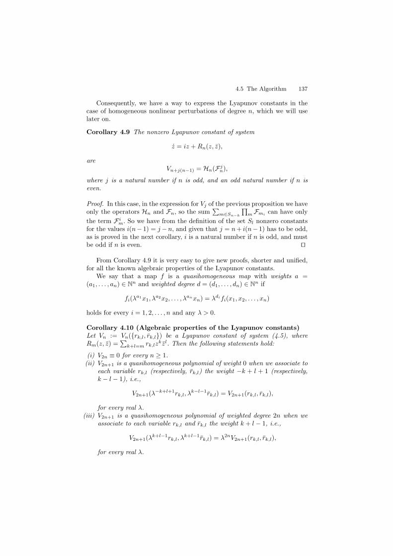
4.5 The Algorithm 137
Consequently, we have a way to express the Lyapunov constants in thecase of homogeneous nonlinear perturbations of degree n, which we will uselater on.
Corollary 4.9 The nonzero Lyapunov constant of system
z = iz + Rn(z, z),
areVn+j(n−1) = Hn(F j
n),
where j is a natural number if n is odd, and an odd natural number if n iseven.
Proof. In this case, in the expression for Vj of the previous proposition we haveonly the operators Hn and Fn, so the sum
∑m∈Sn−k
∏m Fmi
can have only
the term F im. So we have from the definition of the set Sl nonzero constants
for the values i(n− 1) = j −n, and given that j = n + i(n− 1) has to be odd,as is proved in the next corollary, i is a natural number if n is odd, and mustbe odd if n is even. ⊓⊔
From Corollary 4.9 it is very easy to give new proofs, shorter and unified,for all the known algebraic properties of the Lyapunov constants.
We say that a map f is a quasihomogeneous map with weights a =(a1, . . . , an) ∈ Nn and weighted degree d = (d1, . . . , dn) ∈ Nn if
fi(λa1x1, λ
a2x2, . . . , λanxn) = λdifi(x1, x2, . . . , xn)
holds for every i = 1, 2, . . . , n and any λ > 0.
Corollary 4.10 (Algebraic properties of the Lyapunov constants)Let Vn := Vn({rk,l, rk,l}) be a Lyapunov constant of system (4.5), whereRm(z, z) =
∑k+l=m rk,lz
kzl. Then the following statements hold:
(i) V2n ≡ 0 for every n ≥ 1.(ii) V2n+1 is a quasihomogeneous polynomial of weight 0 when we associate to
each variable rk,l (respectively, rk,l) the weight −k + l + 1 (respectively,k − l − 1), i.e.,
V2n+1(λ−k+l+1rk,l, λ
k−l−1rk,l) = V2n+1(rk,l, rk,l),
for every real λ.(iii) V2n+1 is a quasihomogeneous polynomial of weighted degree 2n when we
associate to each variable rk,l and rk,l the weight k + l − 1, i.e.,
V2n+1(λk+l−1rk,l, λ
k+l−1rk,l) = λ2nV2n+1(rk,l, rk,l),
for every real λ.
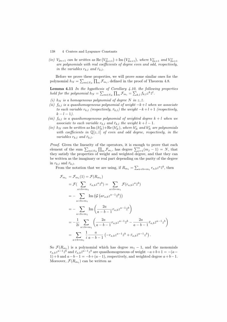
138 4 Centers and Lyapunov Constants
(iv) V2n+1 can be written as Re(V o
2n+1
)+Im
(V e
2n+1
), where V e
2n+1 and V o2n+1
are polynomials with real coefficients of degree even and odd, respectively,in the variables rk,l and rk,l.
Before we prove these properties, we will prove some similar ones for thepolynomial hN =
∑m∈SN
∏m Fmi
, defined in the proof of Theorem 4.8.
Lemma 4.11 In the hypothesis of Corollary 4.10, the following propertieshold for the polynomial hN =
∑m∈SN
∏m Fmi
=∑
k,l fk,lzkzl.
(i) hN is a homogeneous polynomial of degree N in z, z.(ii) fk,l is a quasihomogeneous polynomial of weight −k + l when we associate
to each variable rk,l (respectively, rk,l) the weight −k + l +1 (respectively,k − l − 1).
(iii) fk,l is a quasihomogeneous polynomial of weighted degree k + l when weassociate to each variable rk,l and rk,l the weight k + l − 1.
(iv) hN can be written as Im (hoN )+Re (he
N ), where heN and ho
N are polynomialswith coefficients in Q[z, z] of even and odd degree, respectively, in thevariables rk,l and rk,l.
Proof. Given the linearity of the operators, it is enough to prove that eachelement of the sum
∑m∈SN
∏m Fmi
, has degree∑n
j=1(mj − 1) = N , thatthey satisfy the properties of weight and weighted degree, and that they canbe written as the imaginary or real part depending on the parity of the degreein rk,l and rk,l.
From the notation that we are using, if Rm1=∑
a+b=m1ra,bz
azb, then
Fm1= Fm1
(1) = F(Rm1)
= F(∑
a+b=m1
ra,bzazb) =
∑
a+b=m1
F(ra,bzazb)
= −∑
a+b=m1
Im(G(ara,bz
a−1zb))
= −∑
a+b=m1
Im
(2a
a − b − 1ra,bz
a−1zb
)
= − 1
2i
∑
a+b=m1
(2a
a − b − 1ra,bz
a−1zb − 2a
a − b − 1ra,bz
a−1zb
)
=∑
a+b=m1
1
i
a
a − b − 1
(−ra,bz
a−1zb + ra,bza−1zb
).
So F(Rm1) is a polynomial which has degree m1 − 1, and the monomials
ra,bza−1zb and ra,bz
a−1zb are quasihomogeneous of weight −a+b+1 = −(a−1)+ b and a− b−1 = −b+(a−1), respectively, and weighted degree a+ b−1.Moreover, F(Rm1
) can be written as

4.5 The Algorithm 139
Im
(−
∑
a+b=m1
(2a
a − b − 1ra,bz
a−1zb
)),
and so all statements hold for Rm1.
Suppose now, as an induction hypothesis, that∏n
i=1 Fmi=∑
k,l fk,lzkzl
satisfies the statements of the lemma. Then we have that
n+1∏
j=1
Fmj= Fmn+1
n∏
j=1
Fmj= F
⎛⎜⎝Rmn+1
∑
c+d=∑
n
j=1(mj−1)
fc,dzczd
⎞⎟⎠
= F
⎛⎜⎝
∑
a+b=mn+1
ra,bzazb
∑
c+d=∑
n
j=1(mj−1)
fc,dzczd
⎞⎟⎠
=∑
a+b=mn+1
c+d=∑
n
j=1(mj−1)
F(ra,bfc,dza+czb+d)
= −∑
a+b=mn+1
c+d=∑
n
j=1(mj−1)
Im(G((a + c)ra,bfc,dz
a+c−1zb+d))
= −∑
a+b=mn+1
c+d=∑
n
j=1(mj−1)
Im
(2(a + c)
a + c − 1 − b − dra,bfc,dz
a+c−1zb+d
)
=∑
a+b=mn+1
c+d=∑
n
j=1(mj−1)
(a + c)
a + c − 1 − b − d
1
i
(ra,bfc,dz
a+c−1zb+d−ra,bfc,dza+c−1zb+d)
,
and so∏n+1
j=1 Fmjis a homogeneous polynomial of degree mn+1 +
∑nj=1(mj −
1) − 1 =∑n+1
j=1 (mj − 1) in the variables z, z as statement (i) says.
The coefficients of each monomial in z, z ra,bfc,d and ra,bfc,d, are qua-sihomogeneous of weight −a + b + 1 − c + d = −(a + c − 1) + (b + d) anda − b − 1 + c − d = (a + c − 1) − (b + d), respectively, and weighted degreea + c − 1 + b + d = (a + b − 1) + (c + d), as statements (ii) and (iii) say.
As can be seen in the set of equalities, the operator Fmn, changes with
the parity of the degree of a polynomial in rk,l and rk,l, over the polynomialwhich we operate. From this fact, together with the equalities
Im(A Im(B)) = Re
(−AB − AB
2
),
Im(ARe(B)) = Im
(AB + AB
2
),
we get statement (iv). �
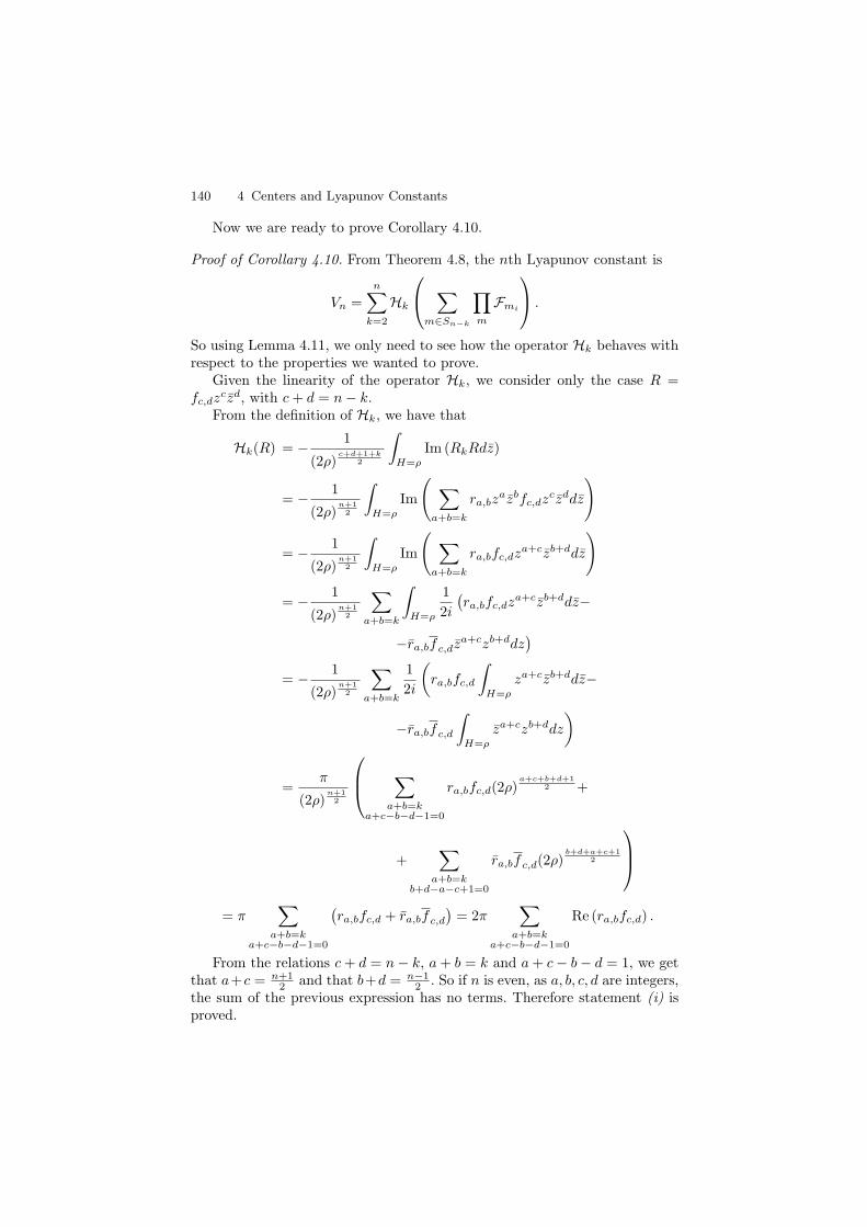
140 4 Centers and Lyapunov Constants
Now we are ready to prove Corollary 4.10.
Proof of Corollary 4.10. From Theorem 4.8, the nth Lyapunov constant is
Vn =
n∑
k=2
Hk
⎛⎝ ∑
m∈Sn−k
∏
m
Fmi
⎞⎠ .
So using Lemma 4.11, we only need to see how the operator Hk behaves withrespect to the properties we wanted to prove.
Given the linearity of the operator Hk, we consider only the case R =fc,dz
czd, with c + d = n − k.From the definition of Hk, we have that
Hk(R) = − 1
(2ρ)c+d+1+k
2
∫
H=ρ
Im (RkRdz)
= − 1
(2ρ)n+1
2
∫
H=ρ
Im
( ∑
a+b=k
ra,bzazbfc,dz
czddz
)
= − 1
(2ρ)n+1
2
∫
H=ρ
Im
( ∑
a+b=k
ra,bfc,dza+czb+ddz
)
= − 1
(2ρ)n+1
2
∑
a+b=k
∫
H=ρ
1
2i
(ra,bfc,dz
a+czb+ddz−
−ra,bfc,dza+czb+ddz
)
= − 1
(2ρ)n+1
2
∑
a+b=k
1
2i
(ra,bfc,d
∫
H=ρ
za+czb+ddz−
−ra,bfc,d
∫
H=ρ
za+czb+ddz
)
=π
(2ρ)n+1
2
⎛⎜⎝
∑
a+b=ka+c−b−d−1=0
ra,bfc,d(2ρ)a+c+b+d+1
2 +
+∑
a+b=kb+d−a−c+1=0
ra,bfc,d(2ρ)b+d+a+c+1
2
⎞⎟⎠
= π∑
a+b=ka+c−b−d−1=0
(ra,bfc,d + ra,bfc,d
)= 2π
∑
a+b=ka+c−b−d−1=0
Re (ra,bfc,d) .
From the relations c + d = n − k, a + b = k and a + c − b − d = 1, we getthat a+c = n+1
2 and that b+d = n−12 . So if n is even, as a, b, c, d are integers,
the sum of the previous expression has no terms. Therefore statement (i) isproved.

4.5 The Algorithm 141
Using Lemma 4.11, we have that Hk(R) is a quasihomogeneous polynomialof weight (−a+b+1)+(−c+d) = 0, and weighted degree (a+b−1)+(c+d) =(k − 1) + (n − k) = n − 1, when the weights of statements (ii) and (iii) areassociated, respectively. This proves these two statements.
In order to prove the last statement, we only need to use the next equalities,
Re(A Im(B)) = Im
(−AB − AB
2
),
Re(ARe(B)) = Re
(AB + AB
2
),
which together with the operator Hk, they change the parity of the degreesof the polynomials in the variables rk,l and rk,l. �
4.5.2 Practical Implementation
In this subsection we describe the algorithm based in Theorem 4.8, whichallows the computation, in a simple way, of the Lyapunov constants for thesystem of differential (4.5). In order to show its speed and easiness of use, wehave evaluated the first five Lyapunov constants for the general system (4.5).In Table 4.1, we give the measure and the computation time of the first four.The computer we have used (a personal computer with Pentium 120 MHzCPU and 32 Mb RAM) has been able to obtain the fifth constant in pieces,but if we try to get the complete expression, the computer crashes.
As far as we know, only the three first constants (V3, V5, V7) for a generalsystem had been found up to now. Moreover, as we will see later on, this isalso an algorithm which allows us to get a new Lyapunov constant using thecomputations done to calculate the previous constants.
Applying this algorithm, the first two Lyapunov constants are:
V3 = H3 + H2(F2),
V5 = H5 + H4(F2) + H3(F2F2) + H2(F4 + F3F2 + F2F3 + F2F2F2),
where, in the computation of V5 we can use the expression of F2, gotten tocompute V3.
Table 4.1. Computation time and measure of the constants of system (4.5)
constant computation time measure in bytes number of monomials
3 0.07 80 45 0.48 1,753 547 11.73 20,864 5269 544.70 17,9897 3,800

142 4 Centers and Lyapunov Constants
In order to compute V7, we need to get the elements of Sk for k = 0, . . . , 5which are
S0 = {(1)},S1 = {(2)},S2 = {(2, 2), (3)},S3 = {(2, 2, 2), (3, 2), (2, 3), (4)},S4 = {(2, 2, 2, 2), (3, 2, 2), (2, 3, 2), (2, 2, 3), (3, 3), (4, 2), (2, 4), (5)},S5 = {(2, 2, 2, 2, 2), (3, 2, 2, 2), (2, 3, 2, 2), (2, 2, 3, 2),
(2, 2, 2, 3), (3, 3, 2), (3, 2, 3), (2, 3, 3), (4, 2, 2), (2, 4, 2),
(2, 2, 4), (4, 3), (3, 4), (5, 2), (2, 5), (6)},
and afterwards, to compute the expressions of∏
m Fmifor every m ∈ Sk. We
must notice that with this method, we may use the expressions of
F2,F2F2,F3F2,F2F3,F2F2F2 and F4,
computed when we got V3 and V5. This allows us to increase the speed ofcomputation of the Lyapunov constants.
As we need a fast method for computing the constants, the best way toobtain the sets Sk is to use an inductive procedure which makes use of theprevious computations. If we define the functions
op(u) := op((u1, . . . , un)) = u1, . . . , un, and
add(a, S) :=⋃
u∈S
{(a, op(u)), (op(u), a)} ,
then we can write
S2 = {(3)}⋃
{add(2, S1)},
S3 = {(4)}⋃
{add(2, S2)}⋃
{add(3, S1)}, and
Sn = {(n)}n−1⋃
k=1
{add(n − k + 1, Sk)}.
The computations done to test this algorithm have been done withMAPLE.
4.6 Applications
In this section we will apply the algorithm to several families of system (4.5).First we will apply it to some families widely studied in the past: quadratic
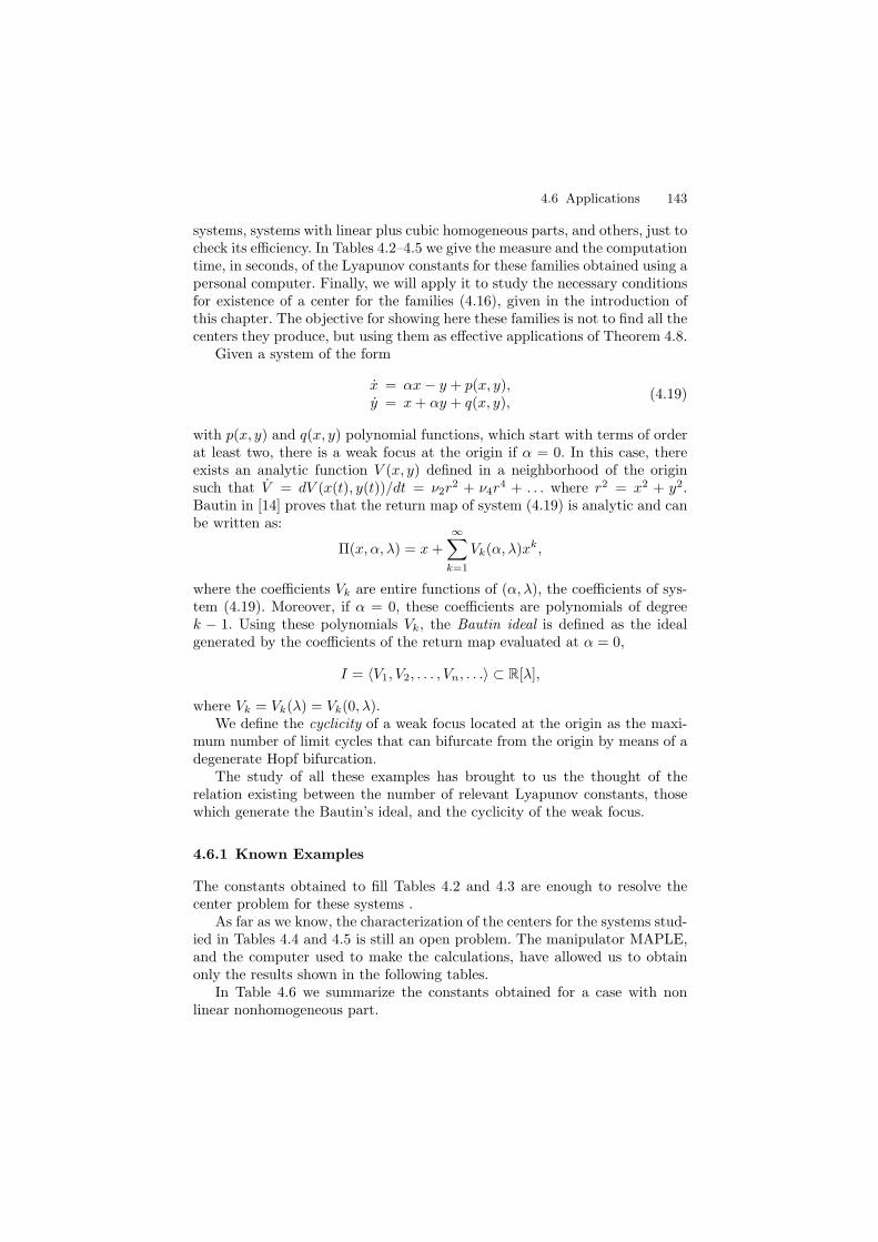
4.6 Applications 143
systems, systems with linear plus cubic homogeneous parts, and others, just tocheck its efficiency. In Tables 4.2–4.5 we give the measure and the computationtime, in seconds, of the Lyapunov constants for these families obtained using apersonal computer. Finally, we will apply it to study the necessary conditionsfor existence of a center for the families (4.16), given in the introduction ofthis chapter. The objective for showing here these families is not to find all thecenters they produce, but using them as effective applications of Theorem 4.8.
Given a system of the form
x = αx − y + p(x, y),y = x + αy + q(x, y),
(4.19)
with p(x, y) and q(x, y) polynomial functions, which start with terms of orderat least two, there is a weak focus at the origin if α = 0. In this case, thereexists an analytic function V (x, y) defined in a neighborhood of the originsuch that V = dV (x(t), y(t))/dt = ν2r
2 + ν4r4 + . . . where r2 = x2 + y2.
Bautin in [14] proves that the return map of system (4.19) is analytic and canbe written as:
Π(x, α, λ) = x +
∞∑
k=1
Vk(α, λ)xk,
where the coefficients Vk are entire functions of (α, λ), the coefficients of sys-tem (4.19). Moreover, if α = 0, these coefficients are polynomials of degreek − 1. Using these polynomials Vk, the Bautin ideal is defined as the idealgenerated by the coefficients of the return map evaluated at α = 0,
I = 〈V1, V2, . . . , Vn, . . .〉 ⊂ R[λ],
where Vk = Vk(λ) = Vk(0, λ).We define the cyclicity of a weak focus located at the origin as the maxi-
mum number of limit cycles that can bifurcate from the origin by means of adegenerate Hopf bifurcation.
The study of all these examples has brought to us the thought of therelation existing between the number of relevant Lyapunov constants, thosewhich generate the Bautin’s ideal, and the cyclicity of the weak focus.
4.6.1 Known Examples
The constants obtained to fill Tables 4.2 and 4.3 are enough to resolve thecenter problem for these systems .
As far as we know, the characterization of the centers for the systems stud-ied in Tables 4.4 and 4.5 is still an open problem. The manipulator MAPLE,and the computer used to make the calculations, have allowed us to obtainonly the results shown in the following tables.
In Table 4.6 we summarize the constants obtained for a case with nonlinear nonhomogeneous part.

144 4 Centers and Lyapunov Constants
Table 4.2. Computation time and measure of the constants of quadratic systemz = iz + R2(z, z). Obviously, we get that v9 = v11 = v13 = 0 if v3, v5, and v7 arezero
constant computation time measure in bytes number of monomials
3 0.21 57 25 0.14 543 147 0.82 2,104 449 4.34 6,075 11011 21.76 14,095 22413 110.95 28,895 414
Table 4.3. Computation time and measure of the constants of cubic system z =iz + R3(z, z). Obviously, we get that v13 = v15 = v17 = 0 if previous constants arealso zero.
constant computation time measure in bytes number of monomials
3 0.03 21 25 0.03 60 27 0.07 281 149 0.33 1,214 3011 1.25 2,895 8213 3.92 7,540 15015 15.15 13,555 30217 49.93 29,979 496
Table 4.4. Computation time and measure of the constants of quartic system z =iz + R4(z, z).
constant computation time measure in bytes number of monomials
7 0.24 114 413 1.04 2,778 6419 33.57 22,796 40425 1,220.26 12,0315 1,684
Finally, we see how far we can reach when we study the system
x = −y + P2(x, y) + P3(x, y),y = x + Q2(x, y) + Q3(x, y),
where the polynomials Pi(x, y) and Qi(x, y) are homogeneous; see Table 4.7.
4.6.2 Kukles-Homogeneous Family
The centers of the homogeneous family
x = −y + Pn(x, y),y = x + Qn(x, y),
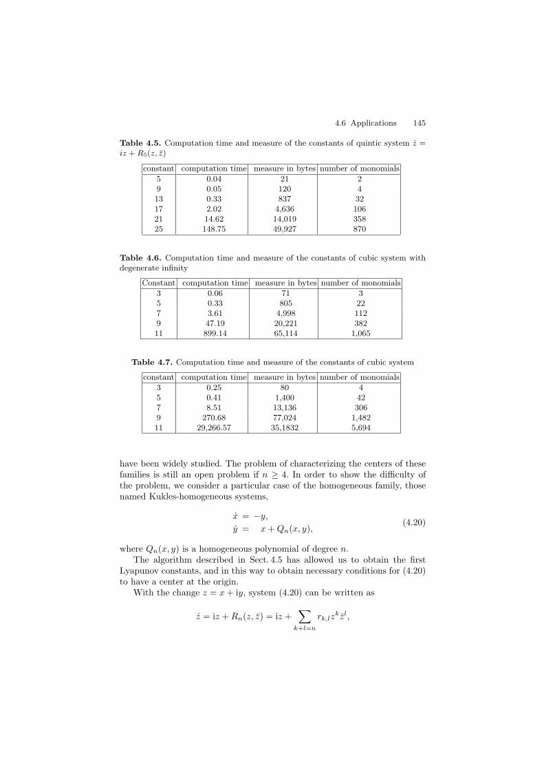
4.6 Applications 145
Table 4.5. Computation time and measure of the constants of quintic system z =iz + R5(z, z)
constant computation time measure in bytes number of monomials
5 0.04 21 29 0.05 120 413 0.33 837 3217 2.02 4,636 10621 14.62 14,019 35825 148.75 49,927 870
Table 4.6. Computation time and measure of the constants of cubic system withdegenerate infinity
Constant computation time measure in bytes number of monomials
3 0.06 71 35 0.33 805 227 3.61 4,998 1129 47.19 20,221 38211 899.14 65,114 1,065
Table 4.7. Computation time and measure of the constants of cubic system
constant computation time measure in bytes number of monomials
3 0.25 80 45 0.41 1,400 427 8.51 13,136 3069 270.68 77,024 1,48211 29,266.57 35,1832 5,694
have been widely studied. The problem of characterizing the centers of thesefamilies is still an open problem if n ≥ 4. In order to show the difficulty ofthe problem, we consider a particular case of the homogeneous family, thosenamed Kukles-homogeneous systems,
x = −y,
y = x + Qn(x, y),(4.20)
where Qn(x, y) is a homogeneous polynomial of degree n.The algorithm described in Sect. 4.5 has allowed us to obtain the first
Lyapunov constants, and in this way to obtain necessary conditions for (4.20)to have a center at the origin.
With the change z = x + iy, system (4.20) can be written as
z = iz + Rn(z, z) = iz +∑
k+l=n
rk,lzkzl,

146 4 Centers and Lyapunov Constants
Table 4.8. Bautin’s number (Bn) and relevant constants (Sn) for system (4.20)
n parameters Bn Sn
2 3 1 13 4 3 34 5 6 55 6 7 5
where rk,l = rl,k. This way, we can apply Theorem 4.8 to calculate the Lya-punov constants.
In the case n = 2, there is only one center condition
v3 = −2ir1,1(r2,0 − r0,2).
If v3 = 0, in [14] it is proved that system (4.20) has a center at the origin.In the case n = 3, there are three conditions for a center,
v3 = −2r2,1 − 2r1,2,
v5 = −4i(r3,0 + r0,3)r1,2,
v7 = 3r3,0r0,3(r3,0 + r0,3).
It is known that these three conditions are sufficient in order that system(4.20) have a center at the origin.
In the cases n = 4, 5, we will not reproduce here the expressions thatwe get for the Lyapunov constants because of their length. We must notethat the method given by Theorem 4.8 has allowed us to obtain the first sixconstants in the case n = 4 and the first eight constants in the case n = 5.The characterization of the centers of these families needs the resolution ofthe system {v4 = v10 = . . . = 0} in the case n = 4 and {v5 = v9 = . . . = 0}in the case n = 5. See Corollary 4.9 where the nonzero constants for thehomogeneous family are given.
With the manipulator MAGMA, we have seen that
(i) The ideal generated by the first k Lyapunov constants is different fromthe one generated by the first k − 1, for k = 2, . . . , 6, when n = 4 and fork = 2, . . . , 7 when n = 5.
(ii) For n = 5, the ideal generated by the first eight constants is the same thatthe one generated by the first seven.
(iii) For n = 4, there exists a natural number k1 such that vk1
6 belongs to theideal generated by the first five constants.
(iv) For n = 5, there exist natural numbers k2 and k3, such that vk2
6 and vk3
7
belong to the ideal generated by the first five constants.
It is natural to think, from this list of properties, that the number ofrelevant Lyapunov constants for cases n = 4 and n = 5 will be 5. These factsare summarized in Table 4.8. In this table, Bn denotes the Bautin’s number
4.7 Bibliographical Comments 147
of the Kukles-homogeneous family of degree n, and the number Sn is a lowerbound on the number of relevant Lyapunov constants.
Table 4.8 has led us to believe that we have enough Lyapunov constantsto obtain all centers of the family defined by system (4.20), but the computerthat we have used has not been able to solve the problem.
4.7 Bibliographical Comments
This chapter has essentially followed the exposition about a new algorithmfor computing the Lyapunov constants due to Gasull and Torregrosa; see [71]and [157] (in catalan).
The study of the stability of a singular point of center-focus type having anon–degenerate linear part for an analytic vector field has generated a largenumber of papers during the twentieth century. As far back as 1893, Lyapunovalready published a paper [105] where a partial solution to this problem wasgiven. He defined the functions which determine the stability, that we now callLyapunov constants. The major difficulty with these functions is their highcomplexity, and to find them explicitly becomes a computational problem.Another problem which has also produced a great quantity of results hasbeen to determine how many limit cycles can bifurcate by perturbing theHamiltonian H = 1
2 (x2 +y2) using analytic functions. For a recent account ondifferent methods that can be used we refer to [27]. Melnikov’s theory based oncalculating the derivative with respect to ε of a return map L(ρ, ε), permits usto give a first answer to this problem. Francoise in [65] developed a new methodin order for obtaining all Melnikov’s functions for this system of differentialequations. Later on, Gasull and Torregrosa [157] used the ideas of Francoisein order to get a new method for calculating the Lyapunov constants of thefirst problem by means of the Melnikov’s functions of the second problem.This new method is good for obtaining both theoretical and practical results.
For a monodromic singular point of an analytic system of differential equa-tions in the plane, there is the well known center-focus problem consisting indetermining whether the singularity is a center or a focus. When the lin-ear part of the system at the singular point has pure imaginary eigenvalues,the problem can be reduced to evaluation of its Lyapunov constants. Farr,Li, Labouriau, and Langford [62] give a summary of the different ways forfinding them. Gasull, Guillamon, and Manosa [69] and Pearson, Lloyd andChristopher [119] contributed to the computation of the Lyapunov constantsand their application to the solution of the center-focus problem. In all theseworks, it is evident that serious computational problems appear, due to theamount of time needed to calculate and also to the fact that the complexityand length of these constants increase largely, not only when we increase thecomplexity of the differential system, but also for a simple systems when wetry to find a Lyapunov constant of large order. In order to reduce these diffi-culties as much as possible, the method of Gasull and Torregrosa provides a
148 4 Centers and Lyapunov Constants
great simplification in time and complexity, and it often allows us to give asimpler proof of known theoretical results. Their method can be generalizedto study the center-focus problem.
One of the main ideas which has allowed the development of this algo-rithm comes from the method given by Francoise in [65], where the successivederivatives of the return map associated to the perturbations of some pla-nar Hamiltonian systems are evaluated. In that paper and in the paper ofFrancoise and Pons [66], the authors apply their method to solve the center-focus problem, but only for systems having homogeneous nonlinear part, andwithout computing explicitly the Lyapunov constants; see also the work ofFrancoise and Yomdin [67]. This generalization has been described also byIliev and Perko [87] and [86].
Using Theorem 4.1, it is not difficult to obtain the expression of the con-stant Vn in terms of words; see Theorem 4.8. For more details about thissubject, the reader may look at the works of Devlin [47] and [48], where theauthor also uses words to study the Lyapunov constants of Abel’s equations;see also Guillamon [78]. From this result, we can obtain the known algebraicproperties of the Lyapunov constants, when they are considered as polynomi-als in the coefficients of system (4.5).
We have mentioned that Corollary 4.9 can be used to provide some newproofs, shorter and unified, of the known algebraic properties of the Lyapunovconstants. Other proofs of these results can be found in the works of Cima,Gasull, Guillamon, Manosa, and Manosas [41], [70] and Zo�ladek [171].
As far as we know, only the three first constants (V3, V5, V7) for a generalsystem had been found up to now; see [69]
More information about the Bautin ideal can be found in Yakovenko [168].See Roussarie [137] for additional results on the cyclicity of a weak focus.The centers described in Sect. 4.6 have been studied by many authors; see
for instance Bautin [14], Chavarriga, and Gine [28–30], Lloyd, Christopher,Devlin, Pearson, and Yasmin [104] and Sibirskii [147].

5
Poincare and Poincare–LyapunovCompactification
In order to study the behavior of the trajectories of a planar differential sys-tem near infinity it is possible to use a compactification. One of the possibleconstructions relies on stereographic projection of the sphere onto the plane,in which case a single “point at infinity” is adjoined to the plane; see Ben-dixson [15]. A better approach for studying the behavior of trajectories nearinfinity is to use the so called Poincare sphere, introduced by Poincare [132].It has the advantage that the singular points at infinity are spread out alongthe equator of the sphere and are therefore of a simpler nature than the sin-gular points of the Bendixson sphere. However, some of the singular points atinfinity on the Poincare sphere may still be very complicated.
In order to improve the construction, we introduce the so called Poincare–Lyapunov sphere, which is however based on a construction of a more ab-stract nature than the previous ones. The singularities are also spread alongthe equator but are in general simpler than for the Poincare sphere. Inthe Poincare–Lyapunov compactification we prefer to work on a hemisphere,calling it as the Poincare–Lyapunov disk, and similarly talk about a Poincaredisk, if we restrict the Poincare sphere to one of the hemispheres separatedby the equator that represents the points at infinity.
5.1 Local Charts
In order to draw the phase portrait of a vector field, we would have to workover the complete real plane R2, which is not very practical. If the functionsdefining the vector field are polynomials, we can apply Poincare compactifica-tion, which will tell us how to draw it in a finite region. Even more, it controlsthe orbits which tend to or come from infinity.
In this chapter we will use (x1, x2) as coordinates on the plane insteadof (x, y).
150 5 Poincare and Poincare–Lyapunov Compactification
Let X = P∂/∂x1 + Q∂/∂x2 be a polynomial vector field (the functions Pand Q are polynomials of arbitrary degree in the variables x1 and x2), or inother words:
x1 = P (x1, x2),
x2 = Q(x1, x2).(5.1)
We recall that the degree of X is d if d is the maximum of the degrees ofP and Q.
Poincare compactification works as follows. First we consider R2 as theplane in R3 defined by (y1, y2, y3) = (x1, x2, 1). We consider the sphere S2 ={y ∈ R3 : y2
1 + y22 + y2
3 = 1} which we will call here Poincare sphere; it istangent to R2 at the point (0, 0, 1). We may divide this sphere into H+ ={y ∈ S2 : y3 > 0} (the northern hemisphere), H− = {y ∈ S2 : y3 < 0}(the southern hemisphere) and S1 = {y ∈ S2 : y3 = 0} (the equator). Nowwe consider the projection of the vector field X from R2 to S2 given by thecentral projections f+ : R2 → S2 and f− : R2 → S2. More precisely, f+(x)(respectively, f−(x)) is the intersection of the straight line passing through thepoint y and the origin with the northern (respectively, southern) hemisphereof S2:
f+(x) =
(x1
Δ(x),
x2
Δ(x),
1
Δ(x)
),
f−(x) =
( −x1
Δ(x),−x2
Δ(x),
−1
Δ(x)
),
where
Δ(x) =√
x21 + x2
2 + 1.
In this way we obtain induced vector fields in each hemisphere. Of course,every induced vector field is analytically conjugate to X. The induced vectorfield on H+ is X(y) = Df+(x)X(x), where y = f+(x), and the one in H− isX(y) = Df−(x)X(x), where y = f−(x). We remark that X is a vector fieldon S2 \ S1 that is everywhere tangent to S2.
We notice that the points at infinity of R2 (two for each direction) are inbijective correspondence with the points of the equator of S2. Now we wouldlike to extend the induced vector field X from S2 \ S1 to S2. Unfortunately itdoes not in general stay bounded as we get close to S1, obstructing the exten-sion. It turns out, however, that if we multiply the vector field by the factorρ(x) = xd−1
3 then as we will check in a moment, the extension becomes possi-ble. The extended vector field on S2 is called the Poincare compactification ofthe vector field X on R2, and it is denoted by p(X). On each hemisphere H+
and H− it is no longer Cω-conjugate to X, but it remains Cω-equivalent. The

5.1 Local Charts 151
technique hence serves well to trace phase portraits, but precautions mustbe taken in making fine calculations, such as eigenvalues at singularities andperiods of closed orbits.
We now work out the construction. As is usual in working with curvedsurfaces, we use charts to make calculations. For S2 we use the six local chartsgiven by Uk = {y ∈ S2 : yk > 0}, Vk = {y ∈ S2 : yk < 0} for k = 1, 2, 3.The corresponding local maps φk : Uk → R2 and ψk : Vk → R2 are definedas φk(y) = −ψk(y) = (ym/yk, yn/yk) for m < n and m,n �= k. We denoteby z = (u, v) the value of φk(y) or ψk(y) for any k, such that (u, v) will playdifferent roles depending on the local chart we are considering. Geometricallythe coordinates (u, v) can be expressed as in Fig. 5.1. The points of S1 in anychart have v = 0.
In what follows we make a detailed calculation of the expression of p(X)only in the local chart U1. We have X(x) = (P (x1, x2), Q(x1, x2)). ThenX(y) = Df+(x)X(x) with y = f+(x) and
Dφ1(y)X(y) = Dφ1(y) ◦ Df+(x)X(x) = D(φ1 ◦ f+)(x)X(x).
Let X|U1denote the system defined as Dφ1(y)X(y). Then since
(φ1 ◦ f+)(x) =
(x2
x1,
1
x1
)= (u, v),
υ
u
u
υ
υ
u
U1
U2
U3
Fig. 5.1. The local charts (Uk, φk) for k = 1, 2, 3 of the Poincare sphere
152 5 Poincare and Poincare–Lyapunov Compactification
we have
X|U1=
⎛⎜⎝−x2
x21
1
x1
− 1
x21
0
⎞⎟⎠
(P (x1, x2)Q(x1, x2)
)
=1
x21
(−x2P (x1, x2) + Q (x1, x2) ,−P (x1, x2))
= v2
(−u
vP
(1
v,u
v
)+
1
vQ
(1
v,u
v
),−P
(1
v,u
v
)).
Now
ρ(y) = yd−13 =
1
Δ(x)d−1=
vd−1
Δ(z)d−1= vd−1m(z),
where m(z) = (1 + u2 + v2)(1−d)/2. Consequently it follows that
ρ(X|U1)(z) = vd+1m(z)
(−u
vP
(1
v,u
v
)+
1
vQ
(1
v,u
v
),−P
(1
v,u
v
)).
In order to prove that the extension of ρX to p(X) is defined on the wholeof S2 we notice that while X|U1
is not well defined when v = 0, p(X)|U1=
ρX|U1is well defined along v = 0, since the multiplying factor vd+1 cancels
any factor of v which could appear in the denominator. Similar argumentscan be applied to the rest of the local charts.
In order to simplify the extended vector field we also make a change in thetime variable and remove the factor m(z). We still keep a vector field on S2
which is Cω-equivalent to X on any of the hemispheres H+ and H−.The expression for p(X) in local chart (U1, φ1) is given by
u = vd
[−uP
(1
v,u
v
)+ Q
(1
v,u
v
)],
v = −vd+1P
(1
v,u
v
).
(5.2)
The expression for (U2, φ2) is
u = vd
[P
(u
v,1
v
)− uQ
(u
v,1
v
)],
v = −vd+1Q
(u
v,1
v
),
(5.3)
and for (U3, φ3) isu = P (u, v),
v = Q(u, v).(5.4)
The expression for p(X) in the charts (Vk, ψk) is the same as for (Uk, φk)multiplied by (−1)d−1, for k = 1, 2, 3.

5.1 Local Charts 153
To study X in the complete plane R2, including its behavior near infinity,it clearly suffices to work on H+ ∪ S1, which we call the Poincare disk. Allcalculation can be done in the three charts (U1, φ1), (U2, φ2), and (U3, φ3) inwhich case the expressions are given by the formulas (5.2), (5.3), and (5.4).
It is clear that we do not need to go through the complete geometricalconstruction, as just presented, in order to get these expressions. The expres-sions in (5.4) clearly do not need any elaboration at all. To obtain (5.2) westart with (5.1) and introduce coordinates (u, v) by the formulas
(x1, x2) = (1
v,u
v). (5.5)
This leads to a vector field Xu which we multiply by vd−1. To obtain (5.3) westart with (5.1) and introduce coordinates (u, v) by the formulas
(x1, x2) = (u
v,1
v). (5.6)
We again multiply the computed vector field Xv by vd−1.This more abstract way of constructing a vector field on a sphere (or
better on a half-sphere) directly by means of charts, is not only the mostpractical way for precise calculations, but also will lead to a generalization(and improvement) of the construction, called the Poincare-Lyapunov disk,as we will see in Sect. 5.3.
Up to Cω-equivalence, the two operations (5.5) and (5.6) can be combinedinto a global construction at infinity:
(x1, x2) = (cos θ
v,sin θ
v), (5.7)
taking θ ∈ S1 and multiplying the vector field again by vd−1. If we work outthis construction we get
θ = v(x2 cos θ − x1 sin θ),
v = −v2(x1 cos θ + x2 sin θ).
This construction is in general preferred in cases where at infinity (on theequator) p(X) has no singularities, implying that the set of points at infinitybecomes a closed orbit. In order to study the behavior of p(X) near that closedorbit, a global study of a neighborhood of it is needed. No such neighborhoodis wholly contained in either chart (U1, φ1) or (U2, φ2).
We remark that in each local chart the local representative of p(X) is apolynomial vector field.
We call finite (respectively, infinite) singular points of X or p(X) the sin-gular points of p(X) which lie in S2 \ S1 (respectively, S1). We note that ify ∈ S1 is an infinite singular point, then −y is also a singular point. Since thelocal behavior near −y is the local behavior near y multiplied by (−1)d−1,
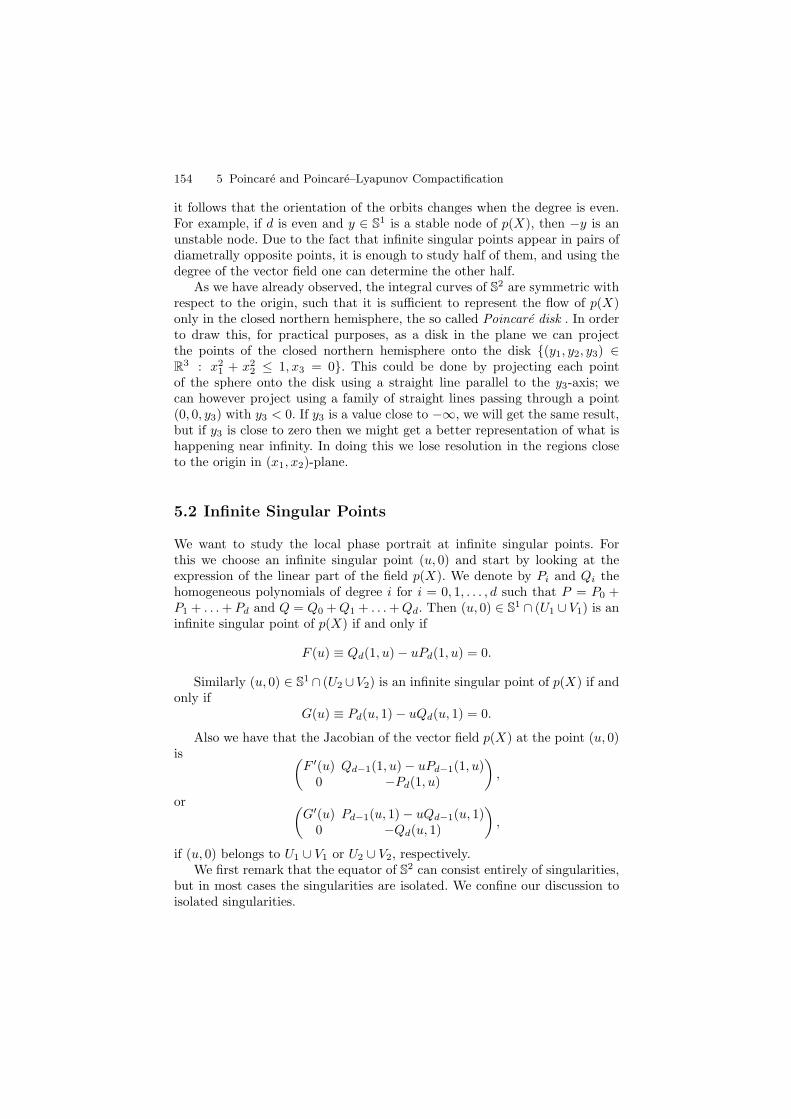
154 5 Poincare and Poincare–Lyapunov Compactification
it follows that the orientation of the orbits changes when the degree is even.For example, if d is even and y ∈ S1 is a stable node of p(X), then −y is anunstable node. Due to the fact that infinite singular points appear in pairs ofdiametrally opposite points, it is enough to study half of them, and using thedegree of the vector field one can determine the other half.
As we have already observed, the integral curves of S2 are symmetric withrespect to the origin, such that it is sufficient to represent the flow of p(X)only in the closed northern hemisphere, the so called Poincare disk . In orderto draw this, for practical purposes, as a disk in the plane we can projectthe points of the closed northern hemisphere onto the disk {(y1, y2, y3) ∈R3 : x2
1 + x22 ≤ 1, x3 = 0}. This could be done by projecting each point
of the sphere onto the disk using a straight line parallel to the y3-axis; wecan however project using a family of straight lines passing through a point(0, 0, y3) with y3 < 0. If y3 is a value close to −∞, we will get the same result,but if y3 is close to zero then we might get a better representation of what ishappening near infinity. In doing this we lose resolution in the regions closeto the origin in (x1, x2)-plane.
5.2 Infinite Singular Points
We want to study the local phase portrait at infinite singular points. Forthis we choose an infinite singular point (u, 0) and start by looking at theexpression of the linear part of the field p(X). We denote by Pi and Qi thehomogeneous polynomials of degree i for i = 0, 1, . . . , d such that P = P0 +P1 + . . . + Pd and Q = Q0 + Q1 + . . . + Qd. Then (u, 0) ∈ S1 ∩ (U1 ∪ V1) is aninfinite singular point of p(X) if and only if
F (u) ≡ Qd(1, u) − uPd(1, u) = 0.
Similarly (u, 0) ∈ S1 ∩ (U2 ∪V2) is an infinite singular point of p(X) if andonly if
G(u) ≡ Pd(u, 1) − uQd(u, 1) = 0.
Also we have that the Jacobian of the vector field p(X) at the point (u, 0)is (
F ′(u) Qd−1(1, u) − uPd−1(1, u)0 −Pd(1, u)
),
or (G′(u) Pd−1(u, 1) − uQd−1(u, 1)
0 −Qd(u, 1)
),
if (u, 0) belongs to U1 ∪ V1 or U2 ∪ V2, respectively.We first remark that the equator of S2 can consist entirely of singularities,
but in most cases the singularities are isolated. We confine our discussion toisolated singularities.
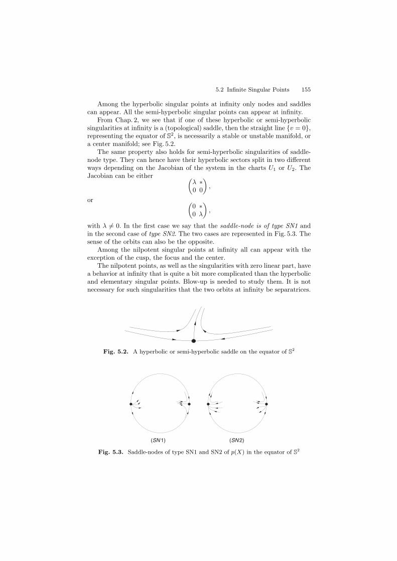
5.2 Infinite Singular Points 155
Among the hyperbolic singular points at infinity only nodes and saddlescan appear. All the semi-hyperbolic singular points can appear at infinity.
From Chap. 2, we see that if one of these hyperbolic or semi-hyperbolicsingularities at infinity is a (topological) saddle, then the straight line {v = 0},representing the equator of S2, is necessarily a stable or unstable manifold, ora center manifold; see Fig. 5.2.
The same property also holds for semi-hyperbolic singularities of saddle-node type. They can hence have their hyperbolic sectors split in two differentways depending on the Jacobian of the system in the charts U1 or U2. TheJacobian can be either (
λ ∗0 0
),
or (0 ∗0 λ
),
with λ �= 0. In the first case we say that the saddle-node is of type SN1 andin the second case of type SN2. The two cases are represented in Fig. 5.3. Thesense of the orbits can also be the opposite.
Among the nilpotent singular points at infinity all can appear with theexception of the cusp, the focus and the center.
The nilpotent points, as well as the singularities with zero linear part, havea behavior at infinity that is quite a bit more complicated than the hyperbolicand elementary singular points. Blow-up is needed to study them. It is notnecessary for such singularities that the two orbits at infinity be separatrices.
Fig. 5.2. A hyperbolic or semi-hyperbolic saddle on the equator of S2
(SN 1) (SN 2)
Fig. 5.3. Saddle-nodes of type SN1 and SN2 of p(X) in the equator of S2

156 5 Poincare and Poincare–Lyapunov Compactification
5.3 Poincare–Lyapunov Compactification
Sometimes, the singularities at infinity in a Poincare compactification arequite complicated, but there is a possibility of simplifying them by workingwith a so called Poincare–Lyapunov compactification. The construction is verysimilar to the one expressed in (5.5) and (5.6) or in (5.7). We start with ageneralization of (5.7), in the sense that we no longer keep the constructionhomogeneous, but make it quasihomogeneous. Thus we set
x1 = cos θ/sα,
x2 = sin θ/sβ ,(5.8)
for some well chosen powers (α, β) ∈ N×N with α, β ≥ 1. If it is advantageousto do so, we can even replace the periodic functions cos θ and sin θ by theperiodic functions Cs θ and Sn θ, which are the unique solutions of the initialvalue problem
d
dθCs θ = −Sn2α−1 θ,
d
dθSn θ = Cs2β−1 θ,
Cs 0 = 1,
Sn 0 = 0,
which satisfy the relation β Sn2α θ + α Cs2β θ = α. It is possible that for asystem for which the usual Poincare compactification has a nonelementarysingular point at infinity, for well chosen α and β, the Poincare–Lyapunovcompactification has only elementary singular points at infinity, or even nosingular points at infinity at all. For the calculations it is again sometimesbetter to work in different charts, comparable to (5.5) and (5.6), and this willbe done in Sect. 9.1.
5.4 Bendixson Compactification
Let X = P∂/∂x1 +Q∂/∂x2 be a polynomial vector field (the functions P andQ are polynomials of maximum degree d). Its associated differential system isgiven by (5.1).
The construction of the Bendixson compactification is as follows (for moredetails see Chapt. 13 of [4]). We consider the sphere in R3 given by y2
1 +y22 + y2
3 = 1/4, and call it the Bendixson sphere. We identify the x1x2-planeon which X is defined with the tangent plane to the sphere at the pointS = (0, 0,−1/2) given by the equation y3 = −1/2. Let pN be the stereographicprojection from the north pole N = (0, 0, 1/2) to the plane y3 = −1/2. Thusp−1
N defines an induced vector field XN on S2 \ N . Clearly the infinity of theplane y3 = −1/2 is transformed by p−1
N into the north pole N .
5.5 Global Flow of a Planar Polynomial Vector Field 157
Now we want to extend XN to a vector field on S2. This extension is calledthe Bendixson compactification and the induced vector field on S2 which hasthe north pole as a singular point is denoted by b(X).
We use two local charts to study the vector field b(X), defined, respectivelyon UN = S2\N and US = S2\S. The corresponding coordinate maps arepN : UN → R2 and pS : US → R2, where pS is the stereographic projection ofS2 from the south pole to the plane y3 = 1/2.
The map pS ◦p−1N from the plane y3 = −1/2 minus S to the plane y3 = 1/2
minus N is given by
u =x1
x21 + x2
2
, v =x2
x21 + x2
2
,
where (u, v) are the coordinates in the plane y3 = 1/2. Hence the infinity ofsystem (5.1) is transformed into the origin of the system
u =1
(u2 + v2)dP (u, v),
v =1
(u2 + v2)dQ(u, v) ,
(5.9)
where P (u, v) = P (x1(u, v), x2(u, v)) and Q(u, v) = Q(x1(u, v), x2(u, v)),whose terms of lowest order are of degree at least d + 2. Finally we intro-duce a change of time scale dt/dτ = (u2 + v2)d and system (5.9) becomes
u = P (u, v),
v = Q(u, v),(5.10)
where u = du/dτ and v = dv/dτ . Since d + 2 is the minimum of the degrees
of the homogeneous parts of P (u, v) and Q(u, v) it is clear that (0, 0) is asingular point of system (5.10).
5.5 Global Flow of a Planar Polynomial Vector Field
First, we determine the phase portrait on the Poincare disk of the system
x = x,
y = −y.(5.11)
This system has a unique finite singular point, the origin, which is a saddle.Let X be the vector field associated to system (5.11). Then the expression forp(X) in the local chart U1 is
u = −2u,
v = −v.
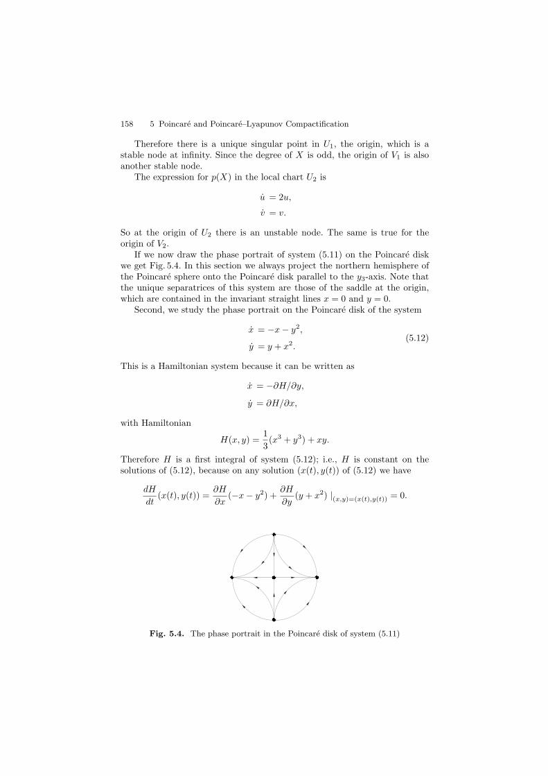
158 5 Poincare and Poincare–Lyapunov Compactification
Therefore there is a unique singular point in U1, the origin, which is astable node at infinity. Since the degree of X is odd, the origin of V1 is alsoanother stable node.
The expression for p(X) in the local chart U2 is
u = 2u,
v = v.
So at the origin of U2 there is an unstable node. The same is true for theorigin of V2.
If we now draw the phase portrait of system (5.11) on the Poincare diskwe get Fig. 5.4. In this section we always project the northern hemisphere ofthe Poincare sphere onto the Poincare disk parallel to the y3-axis. Note thatthe unique separatrices of this system are those of the saddle at the origin,which are contained in the invariant straight lines x = 0 and y = 0.
Second, we study the phase portrait on the Poincare disk of the system
x = −x − y2,
y = y + x2.(5.12)
This is a Hamiltonian system because it can be written as
x = −∂H/∂y,
y = ∂H/∂x,
with Hamiltonian
H(x, y) =1
3(x3 + y3) + xy.
Therefore H is a first integral of system (5.12); i.e., H is constant on thesolutions of (5.12), because on any solution (x(t), y(t)) of (5.12) we have
dH
dt(x(t), y(t)) =
∂H
∂x(−x − y2) +
∂H
∂y(y + x2) |(x,y)=(x(t),y(t)) = 0.
Fig. 5.4. The phase portrait in the Poincare disk of system (5.11)
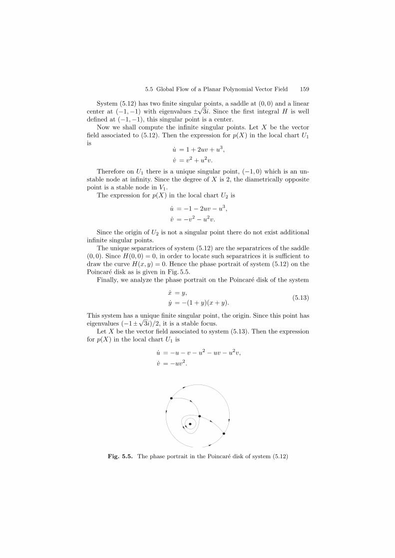
5.5 Global Flow of a Planar Polynomial Vector Field 159
System (5.12) has two finite singular points, a saddle at (0, 0) and a linearcenter at (−1,−1) with eigenvalues
√3i. Since the first integral H is well
defined at (−1,−1), this singular point is a center.Now we shall compute the infinite singular points. Let X be the vector
field associated to (5.12). Then the expression for p(X) in the local chart U1
isu = 1 + 2uv + u3,
v = v2 + u2v.
Therefore on U1 there is a unique singular point, (−1, 0) which is an un-stable node at infinity. Since the degree of X is 2, the diametrically oppositepoint is a stable node in V1.
The expression for p(X) in the local chart U2 is
u = −1 − 2uv − u3,
v = −v2 − u2v.
Since the origin of U2 is not a singular point there do not exist additionalinfinite singular points.
The unique separatrices of system (5.12) are the separatrices of the saddle(0, 0). Since H(0, 0) = 0, in order to locate such separatrices it is sufficient todraw the curve H(x, y) = 0. Hence the phase portrait of system (5.12) on thePoincare disk as is given in Fig. 5.5.
Finally, we analyze the phase portrait on the Poincare disk of the system
x = y,
y = −(1 + y)(x + y).(5.13)
This system has a unique finite singular point, the origin. Since this point haseigenvalues (−1
√3i)/2, it is a stable focus.
Let X be the vector field associated to system (5.13). Then the expressionfor p(X) in the local chart U1 is
u = −u − v − u2 − uv − u2v,
v = −uv2.
Fig. 5.5. The phase portrait in the Poincare disk of system (5.12)
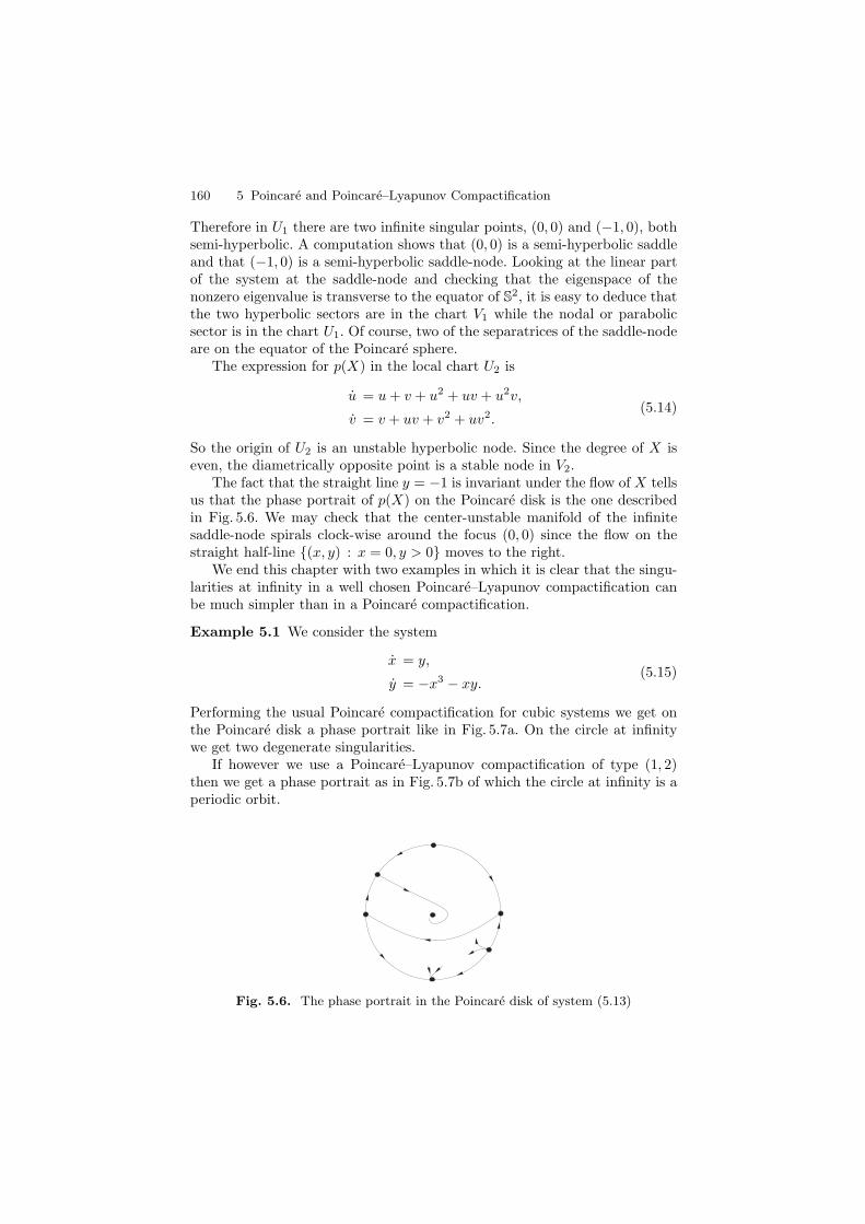
160 5 Poincare and Poincare–Lyapunov Compactification
Therefore in U1 there are two infinite singular points, (0, 0) and (−1, 0), bothsemi-hyperbolic. A computation shows that (0, 0) is a semi-hyperbolic saddleand that (−1, 0) is a semi-hyperbolic saddle-node. Looking at the linear partof the system at the saddle-node and checking that the eigenspace of thenonzero eigenvalue is transverse to the equator of S2, it is easy to deduce thatthe two hyperbolic sectors are in the chart V1 while the nodal or parabolicsector is in the chart U1. Of course, two of the separatrices of the saddle-nodeare on the equator of the Poincare sphere.
The expression for p(X) in the local chart U2 is
u = u + v + u2 + uv + u2v,
v = v + uv + v2 + uv2.(5.14)
So the origin of U2 is an unstable hyperbolic node. Since the degree of X iseven, the diametrically opposite point is a stable node in V2.
The fact that the straight line y = −1 is invariant under the flow of X tellsus that the phase portrait of p(X) on the Poincare disk is the one describedin Fig. 5.6. We may check that the center-unstable manifold of the infinitesaddle-node spirals clock-wise around the focus (0, 0) since the flow on thestraight half-line {(x, y) : x = 0, y > 0} moves to the right.
We end this chapter with two examples in which it is clear that the singu-larities at infinity in a well chosen Poincare–Lyapunov compactification canbe much simpler than in a Poincare compactification.
Example 5.1 We consider the system
x = y,
y = −x3 − xy.(5.15)
Performing the usual Poincare compactification for cubic systems we get onthe Poincare disk a phase portrait like in Fig. 5.7a. On the circle at infinitywe get two degenerate singularities.
If however we use a Poincare–Lyapunov compactification of type (1, 2)then we get a phase portrait as in Fig. 5.7b of which the circle at infinity is aperiodic orbit.
Fig. 5.6. The phase portrait in the Poincare disk of system (5.13)
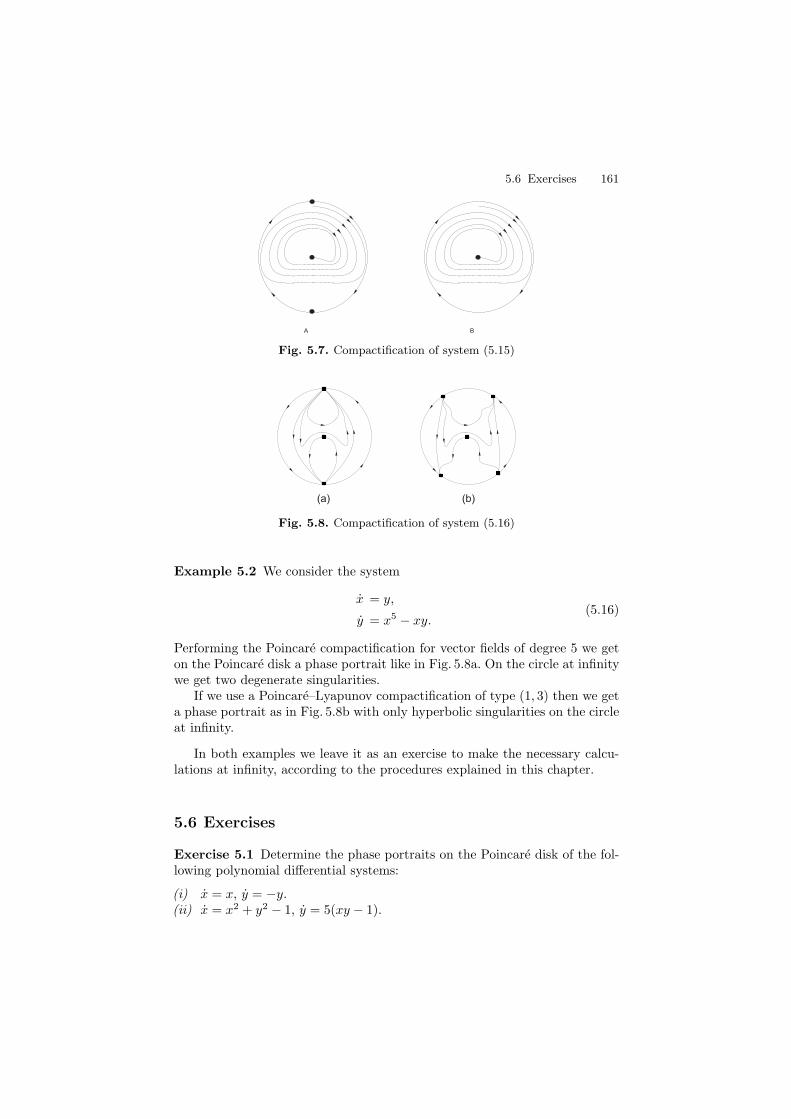
5.6 Exercises 161
Fig. 5.7. Compactification of system (5.15)
(a) (b)
Fig. 5.8. Compactification of system (5.16)
Example 5.2 We consider the system
x = y,
y = x5 − xy.(5.16)
Performing the Poincare compactification for vector fields of degree 5 we geton the Poincare disk a phase portrait like in Fig. 5.8a. On the circle at infinitywe get two degenerate singularities.
If we use a Poincare–Lyapunov compactification of type (1, 3) then we geta phase portrait as in Fig. 5.8b with only hyperbolic singularities on the circleat infinity.
In both examples we leave it as an exercise to make the necessary calcu-lations at infinity, according to the procedures explained in this chapter.
5.6 Exercises
Exercise 5.1 Determine the phase portraits on the Poincare disk of the fol-lowing polynomial differential systems:
(i) x = x, y = −y.(ii) x = x2 + y2 − 1, y = 5(xy − 1).

162 5 Poincare and Poincare–Lyapunov Compactification
(a)
(d) (e)
(f) (g)
(b) (c)
Fig. 5.9. Phase portraits of Exercise 5.2
(iii) x = −y(1+x)+αx+(α+1)x2, y = x(1+x), depending on the parameterα ∈ (0, 1).
Exercise 5.2 Determine which of the global phase portraits shown in Fig. 5.9correspond to the following quadratic systems (two of them do not correspondto any system presented).
(i) x = −4y + 2xy − 8, y = 4y2 − x2.(ii) x = 2x − 2xy, y = 2y − x2 + y2.(iii) x = −x2 − y2 + 1, y = 2x.(iv) x = −x2 − y2 + 1, y = 2xy.(v) x = x2 − y2 − 1, y = 2y.
Exercise 5.3 Consider a homogeneous quadratic differential system:
x = ax2 + bxy + cy2,
y = dx2 + exy + fy2.
Supposing that the singular point at the origin is isolated, hence unique, showthat the phase portrait on the Poincare disk must be one of the seven phaseportraits given in Fig. 5.10.
5.7 Bibliographical Comments
For more information on Poincare compactification; see the book of Andronov,Leontovich, Gordon and Maier [4], the book of Sotomayor [151] and the paperof Gonzalez [76].

5.7 Bibliographical Comments 163
Fig. 5.10. Phase portraits of quadratic homogenous systems
The use of a quasihomogeneous compactification of polynomial planar vec-tor fields and the related name Poincare–Lyapunov compactification were in-troduced in papers of Dumortier at the end of the eighties. The inspirationcame from the strongly related quasihomogeneous blow-up of singularities, aspresented in Chap. 3. As one application among others, a systematic study bymeans of the technique has been made of all polynomial Lienard equationsnear infinity [55]


6
Indices of Planar Singular Points
In this chapter we study the index of a singular point of a vector field on R2 oron S2. For a given vector field X on S2 having finitely many singular points, weshall see that the sum of their indices is equal to 2 (the Euler characteristicof S2). This result is the famous Poincare Index Theorem, which later onwas extended by Hopf to vector fields on compact manifolds. We also provethe formula of Poincare for computing the index of an isolated singularity.Finally we briefly discuss the relation between the index and the multiplicityof a singular point.
6.1 Index of a Closed Path Around a Point
A path in the plane R2 is a continuous map from the interval I = [0, 1] to R2
(σ : I → R2); that is, we assign to every t ∈ [0, 1] the point σ(t) = (σ1(t), σ2(t))in the plane, such that σi : I → R are continuous maps.
The point σ(0) is called the origin of the path σ and σ(1) is called theendpoint of the path. We must not confuse a path with its image σ(I) ⊂ R2;σ(I) is called a curve. For example, the paths σ : σ(t) = (r cos πt, r sin πt) andτ : τ(t) = (r(1−2t), 2r
√t(1 − t)), are obviously different, but the curves σ(I)
and τ(I) coincide; see Fig. 6.1.Let q be a point of R2 which does not belong to σ(I) and let r be a ray
with origin at q. For every point σ(t) we denote by ϕ(t) the angle formedby the rays r and qσ(t). The angle ϕ(t) is an element of the circle R/2πZ.The function ϕ : I → R/2πZ is continuous with respect to the parameter t;see Fig. 6.2. We can cover it by a continuous mapping ϕ : I → R. From nowon we shall work with such a continuous cover, with the extra condition thatϕ(0) = 0. We call ϕ an angle function.
A closed path is a path whose endpoint coincides with its origin (i.e.,σ(1) = σ(0)). Equivalently, a closed path can be considered as a continuousmap σ : S1 → R2. Let q be a point of R2 which does not belong to σ(I). Then
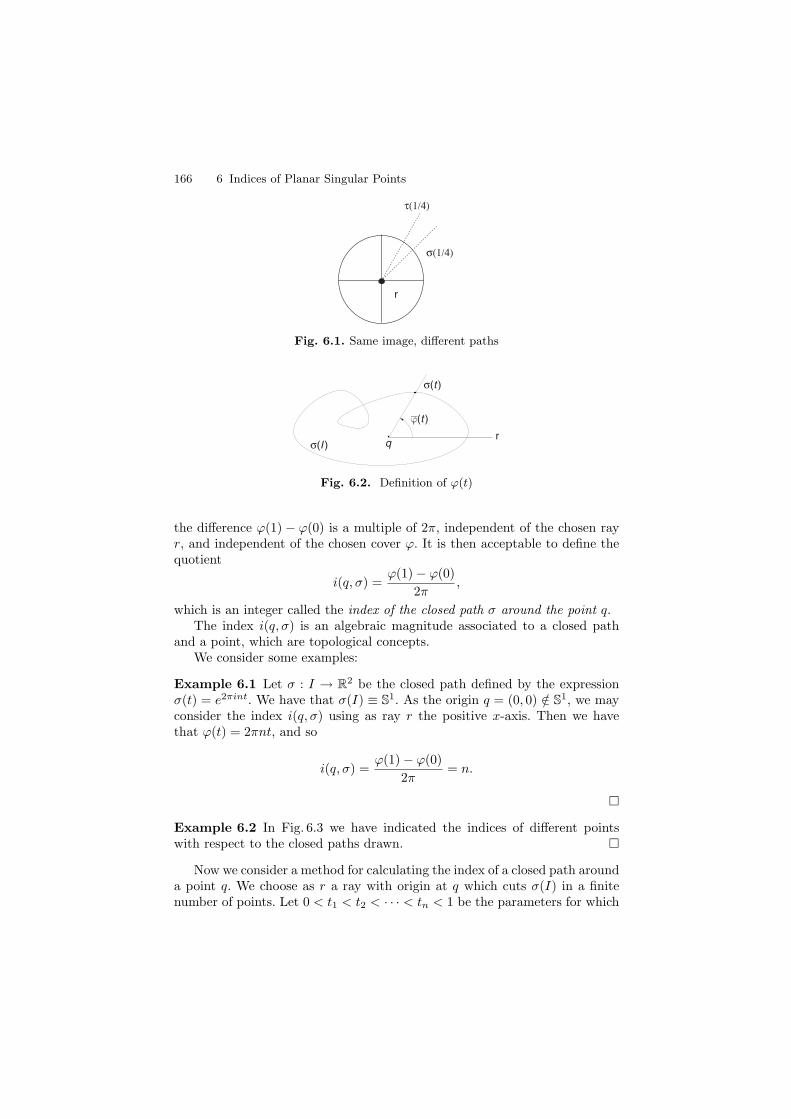
166 6 Indices of Planar Singular Points
r
τ(1/4)
σ(1/4)
Fig. 6.1. Same image, different paths
r
σ(t )
σ(I ) q
ϕ(t )−
Fig. 6.2. Definition of ϕ(t)
the difference ϕ(1) − ϕ(0) is a multiple of 2π, independent of the chosen rayr, and independent of the chosen cover ϕ. It is then acceptable to define thequotient
i(q, σ) =ϕ(1) − ϕ(0)
2π,
which is an integer called the index of the closed path σ around the point q.The index i(q, σ) is an algebraic magnitude associated to a closed path
and a point, which are topological concepts.We consider some examples:
Example 6.1 Let σ : I → R2 be the closed path defined by the expressionσ(t) = e2πint. We have that σ(I) ≡ S1. As the origin q = (0, 0) /∈ S1, we mayconsider the index i(q, σ) using as ray r the positive x-axis. Then we havethat ϕ(t) = 2πnt, and so
i(q, σ) =ϕ(1) − ϕ(0)
2π= n.
�
Example 6.2 In Fig. 6.3 we have indicated the indices of different pointswith respect to the closed paths drawn. �
Now we consider a method for calculating the index of a closed path arounda point q. We choose as r a ray with origin at q which cuts σ(I) in a finitenumber of points. Let 0 < t1 < t2 < · · · < tn < 1 be the parameters for which
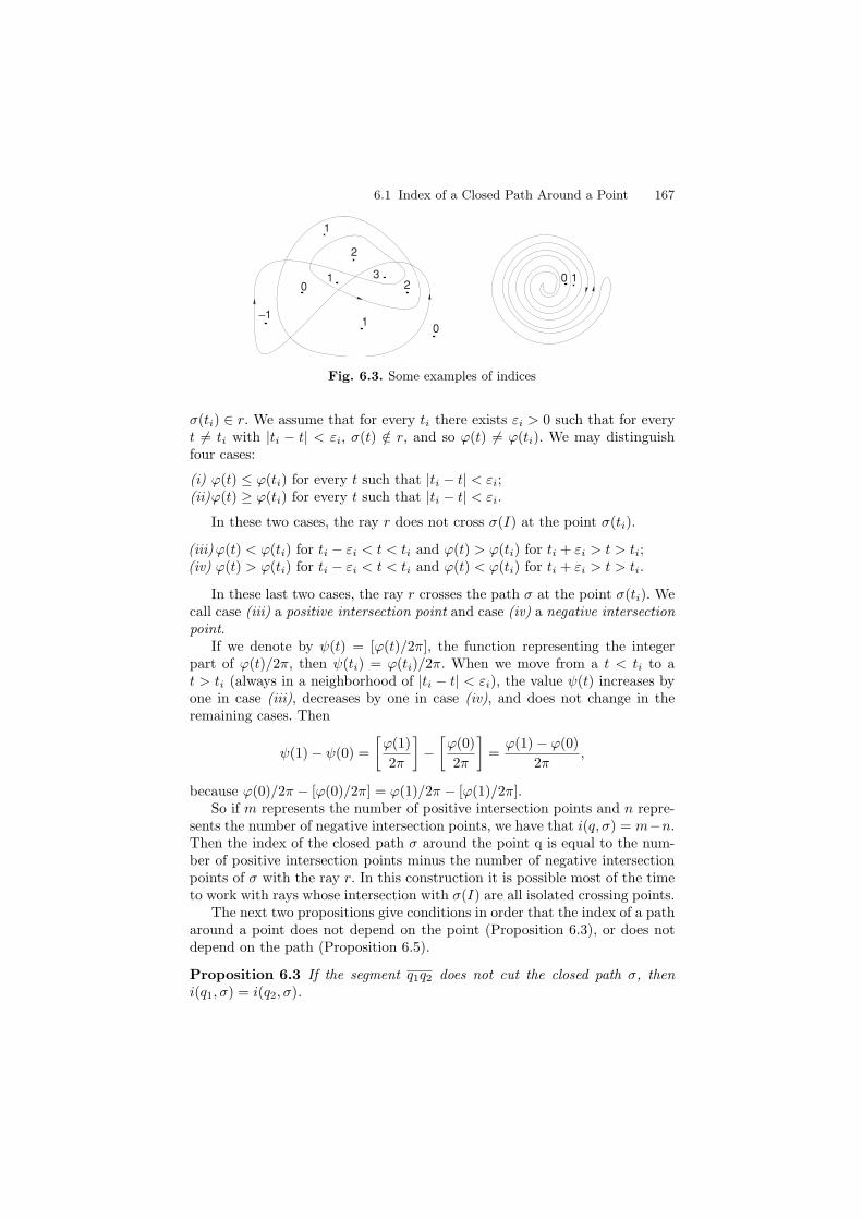
6.1 Index of a Closed Path Around a Point 167
0 1
10
1
2
32
10
−1
Fig. 6.3. Some examples of indices
σ(ti) ∈ r. We assume that for every ti there exists εi > 0 such that for everyt �= ti with |ti − t| < εi, σ(t) /∈ r, and so ϕ(t) �= ϕ(ti). We may distinguishfour cases:
(i) ϕ(t) ≤ ϕ(ti) for every t such that |ti − t| < εi;(ii)ϕ(t) ≥ ϕ(ti) for every t such that |ti − t| < εi.
In these two cases, the ray r does not cross σ(I) at the point σ(ti).
(iii)ϕ(t) < ϕ(ti) for ti − εi < t < ti and ϕ(t) > ϕ(ti) for ti + εi > t > ti;(iv) ϕ(t) > ϕ(ti) for ti − εi < t < ti and ϕ(t) < ϕ(ti) for ti + εi > t > ti.
In these last two cases, the ray r crosses the path σ at the point σ(ti). Wecall case (iii) a positive intersection point and case (iv) a negative intersectionpoint.
If we denote by ψ(t) = [ϕ(t)/2π], the function representing the integerpart of ϕ(t)/2π, then ψ(ti) = ϕ(ti)/2π. When we move from a t < ti to at > ti (always in a neighborhood of |ti − t| < εi), the value ψ(t) increases byone in case (iii), decreases by one in case (iv), and does not change in theremaining cases. Then
ψ(1) − ψ(0) =
[ϕ(1)
2π
]−[ϕ(0)
2π
]=
ϕ(1) − ϕ(0)
2π,
because ϕ(0)/2π − [ϕ(0)/2π] = ϕ(1)/2π − [ϕ(1)/2π].So if m represents the number of positive intersection points and n repre-
sents the number of negative intersection points, we have that i(q, σ) = m−n.Then the index of the closed path σ around the point q is equal to the num-ber of positive intersection points minus the number of negative intersectionpoints of σ with the ray r. In this construction it is possible most of the timeto work with rays whose intersection with σ(I) are all isolated crossing points.
The next two propositions give conditions in order that the index of a patharound a point does not depend on the point (Proposition 6.3), or does notdepend on the path (Proposition 6.5).
Proposition 6.3 If the segment q1q2 does not cut the closed path σ, theni(q1, σ) = i(q2, σ).

168 6 Indices of Planar Singular Points
Proof. Let σ : I → R2 be a closed path, and q1 and q2 two points not belongingto σ(I). Let ϕ1 and ϕ2 be angle functions with respect to q1 and q2. Then thefunction
δ(t) =ϕ1(t) − ϕ2(t)
π
is continuous for every t, and we have that
δ(1) − δ(0) =ϕ1(1) − ϕ2(1)
π− ϕ1(0) − ϕ2(0)
π= 2(i(q1, σ) − i(q2, σ)).
Suppose that i(q1, σ) �= i(q2, σ). Then we have that |δ(1) − δ(0)| ≥ 2, andby the Intermediate Value Theorem, there exists t0 ∈ I such that δ(t0) is odd,that is ϕ1(t0) − ϕ2(t0) = nπ with n odd.
But if we choose parallel rays with origins at q1 and q2 to define ϕ1 andϕ2, respectively, in such a way that the ray starting at q1 passes through q2 ,then σ(t0) ∈ q1q2, which contradicts the conditions of the proposition. �
Corollary 6.4 If q1 and q2 belong to the same connected component of R2 \σ(I), then i(q1, σ) = i(q2, σ).
Proposition 6.5 Let σ1, σ2 : I → R2 be closed paths and q ∈ R2 such thatfor every t ∈ I we have q /∈ σ1(t)σ2(t). Then i(q, σ1) = i(q, σ2).
Proof. Let ϕ1 and ϕ2 be angle functions with respect to σ1 and σ2 and thepoint q. If we suppose that the indices are different, then by the same argu-ments as in Proposition 6.3, there exists a t0 such that ϕ1(t0) − ϕ2(t0) = nπwith n odd.
But this implies that q belongs to a segment determined by σ1(t0) andσ2(t0), contradicting the hypothesis. �
Corollary 6.6 Let σ1, σ2 : I → R2 be closed paths and q ∈ R2 such thatq /∈ σ1(I) ∪ σ2(I). If for every t ∈ I we have ‖σ1(t) − σ2(t)‖ < ‖q − σ1(t)‖,then i(q, σ1) = i(q, σ2).
Proof. Under the hypotheses of the corollary, q /∈ σ1(t)σ2(t) for any t ∈ I.Then Proposition 6.5 applies. �
6.2 Deformations of Paths
Given a family of closed paths σs : I → R2, with s ∈ I, we say that we havea deformation of closed paths if σ(s, t) = σs(t) depend continuously on thevariables t ∈ I and s ∈ I.
Two closed paths which can be deformed one into the other, as we havedescribed, are called homotopic closed paths; see Fig. 6.4.
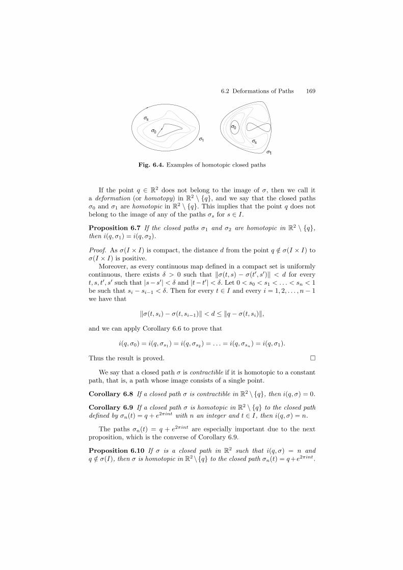
6.2 Deformations of Paths 169
s1
s1
s0
s0
ss
ss
Fig. 6.4. Examples of homotopic closed paths
If the point q ∈ R2 does not belong to the image of σ, then we call ita deformation (or homotopy) in R2 \ {q}, and we say that the closed pathsσ0 and σ1 are homotopic in R2 \ {q}. This implies that the point q does notbelong to the image of any of the paths σs for s ∈ I.
Proposition 6.7 If the closed paths σ1 and σ2 are homotopic in R2 \ {q},then i(q, σ1) = i(q, σ2).
Proof. As σ(I × I) is compact, the distance d from the point q /∈ σ(I × I) toσ(I × I) is positive.
Moreover, as every continuous map defined in a compact set is uniformlycontinuous, there exists δ > 0 such that ‖σ(t, s) − σ(t′, s′)‖ < d for everyt, s, t′, s′ such that |s− s′| < δ and |t− t′| < δ. Let 0 < s0 < s1 < . . . < sn < 1be such that si − si−1 < δ. Then for every t ∈ I and every i = 1, 2, . . . , n − 1we have that
‖σ(t, si) − σ(t, si−1)‖ < d ≤ ‖q − σ(t, si)‖,
and we can apply Corollary 6.6 to prove that
i(q, σ0) = i(q, σs1) = i(q, σs2
) = . . . = i(q, σsn) = i(q, σ1).
Thus the result is proved. �
We say that a closed path σ is contractible if it is homotopic to a constantpath, that is, a path whose image consists of a single point.
Corollary 6.8 If a closed path σ is contractible in R2 \ {q}, then i(q, σ) = 0.
Corollary 6.9 If a closed path σ is homotopic in R2 \ {q} to the closed pathdefined by σn(t) = q + e2πint with n an integer and t ∈ I, then i(q, σ) = n.
The paths σn(t) = q + e2πint are especially important due to the nextproposition, which is the converse of Corollary 6.9.
Proposition 6.10 If σ is a closed path in R2 such that i(q, σ) = n andq /∈ σ(I), then σ is homotopic in R2 \{q} to the closed path σn(t) = q+e2πint.
170 6 Indices of Planar Singular Points
Proof. We choose as r the right horizontal ray passing through the point q.Let ϕ(t) be an angle function for the path σ with respect to the point q. Weset d(t) = ‖q − σ(t)‖, and define then σ : I × I → R2 by
σ(t, s) = q + [d(t)(1 − s) + s]e(ϕ(t)(1−s)+2πnst)i.
It is clear that σ is a continuous map, that σ(t, 0) = σ(t), and that σ(t, 1) =σn(t). Moreover, as ϕ(1) = ϕ(0) + 2πn, σ(0, s) = σ(1, s) for every s. Finally,as q /∈ σ(I × I), σ gives the required deformation. �
This proposition can be completed to the next theorem.
Theorem 6.11 Two closed paths are homotopic in R2 \ {q} if and only ifthey have the same index around q.
Corollary 6.12 If σ : I → R2 \ {q} is a path with i(q, σ) = 0, then thereexists a map f : D
2 → R2 \ {q} with f(e2πit) = σ(t).
6.3 Continuous Maps of the Closed Disk
A closed path σ : I → R2 can also be considered as a continuous map σ :S1 → R2 and conversely by the relation σ(e2πit) = σ(t). If no confusion ispossible we also simply write σ instead of σ.
Let D2 be the closed disk of radius one centered at the origin and let
f : D2 → R2 be a continuous map expressed in polar coordinates as f(r, θ).
The boundary of D2 is the circle S1. The restriction of f to S1 is the closed
path σ : S1 → R2. If q ∈ R2 does not belong to the image of f , then the map
σ : I × I −→R2
(t, s) → f(1 − s, 2πt)
provides a deformation from the closed path σ, with σ(t) = f(1, 2πt), to aconstant path. So the closed path σ is contractible due to Corollary 6.8 andconsequently i(q, σ) = 0. In short, we have proved the following result.
Theorem 6.13 Let f : D2 → R2 be a continuous map, and let q be a point
of R2 which does not belong to f(S1), and such that i(q, σ) �= 0, with σ(t) =f(1, 2πt) as above. Then q ∈ f(D2).
This theorem can be thought of as an extension of the Intermediate ValueTheorem from the interval I to the disk D
2.
6.4 Vector Fields Along the Unit Circle
We consider a continuous vector field X defined on the circle S1. Given a pointp = e2πit ∈ S1, we identify the vector X(p) = (X1(p), X2(p)) with the point
σ(t) ∈ R2 such that−−−→0σ(t) = X(p). This allows us to define a continuous map
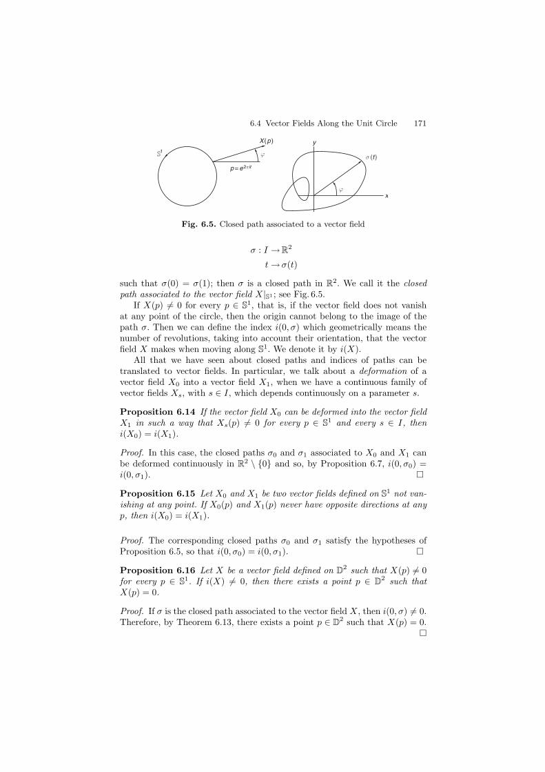
6.4 Vector Fields Along the Unit Circle 171
ϕ
σ (t )
X (p )
p = e2πit
x
y
ϕ1
Fig. 6.5. Closed path associated to a vector field
σ : I →R2
t →σ(t)
such that σ(0) = σ(1); then σ is a closed path in R2. We call it the closedpath associated to the vector field X|S1 ; see Fig. 6.5.
If X(p) �= 0 for every p ∈ S1, that is, if the vector field does not vanishat any point of the circle, then the origin cannot belong to the image of thepath σ. Then we can define the index i(0, σ) which geometrically means thenumber of revolutions, taking into account their orientation, that the vectorfield X makes when moving along S1. We denote it by i(X).
All that we have seen about closed paths and indices of paths can betranslated to vector fields. In particular, we talk about a deformation of avector field X0 into a vector field X1, when we have a continuous family ofvector fields Xs, with s ∈ I, which depends continuously on a parameter s.
Proposition 6.14 If the vector field X0 can be deformed into the vector fieldX1 in such a way that Xs(p) �= 0 for every p ∈ S1 and every s ∈ I, theni(X0) = i(X1).
Proof. In this case, the closed paths σ0 and σ1 associated to X0 and X1 canbe deformed continuously in R2 \ {0} and so, by Proposition 6.7, i(0, σ0) =i(0, σ1). �
Proposition 6.15 Let X0 and X1 be two vector fields defined on S1 not van-ishing at any point. If X0(p) and X1(p) never have opposite directions at anyp, then i(X0) = i(X1).
Proof. The corresponding closed paths σ0 and σ1 satisfy the hypotheses ofProposition 6.5, so that i(0, σ0) = i(0, σ1). �
Proposition 6.16 Let X be a vector field defined on D2 such that X(p) �= 0
for every p ∈ S1. If i(X) �= 0, then there exists a point p ∈ D2 such that
X(p) = 0.
Proof. If σ is the closed path associated to the vector field X, then i(0, σ) �= 0.Therefore, by Theorem 6.13, there exists a point p ∈ D
2 such that X(p) = 0.�
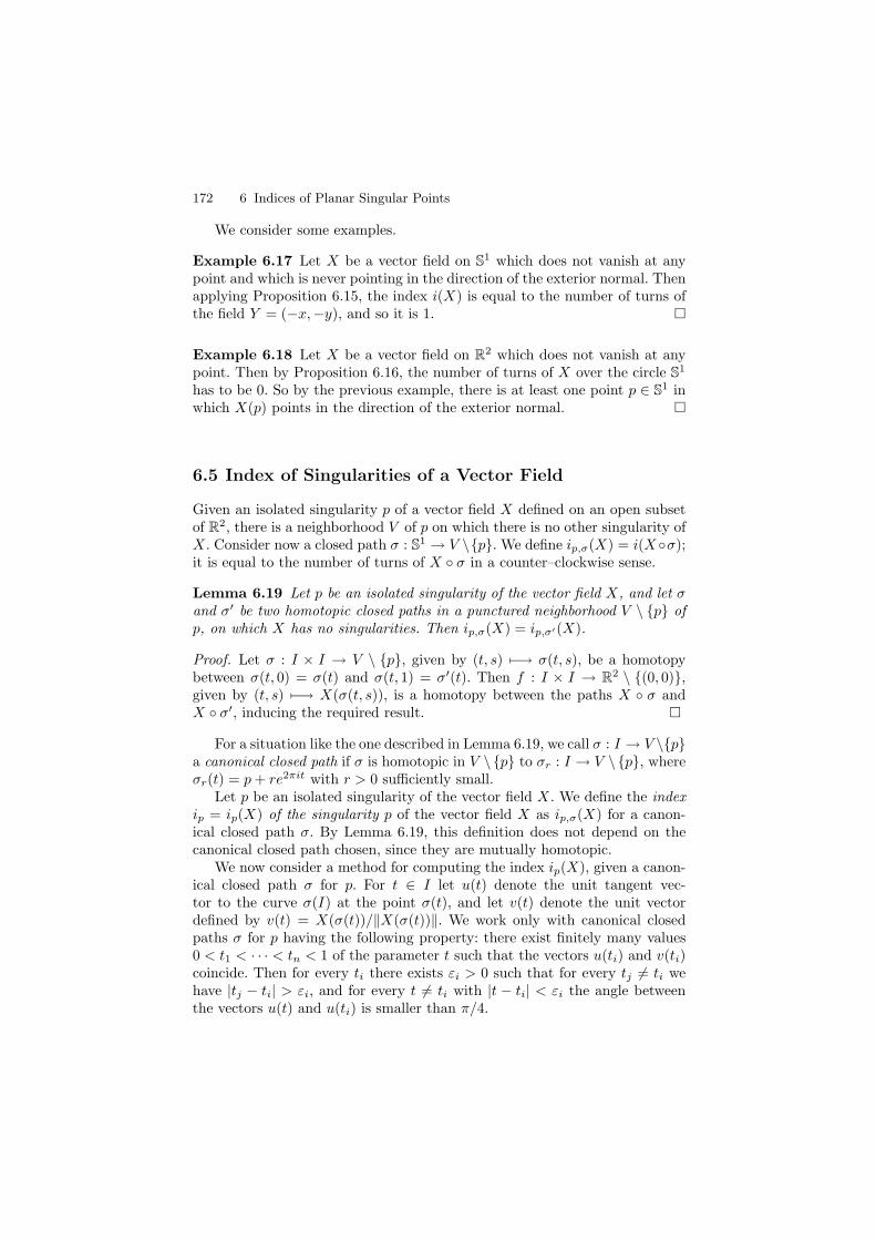
172 6 Indices of Planar Singular Points
We consider some examples.
Example 6.17 Let X be a vector field on S1 which does not vanish at anypoint and which is never pointing in the direction of the exterior normal. Thenapplying Proposition 6.15, the index i(X) is equal to the number of turns ofthe field Y = (−x,−y), and so it is 1. �
Example 6.18 Let X be a vector field on R2 which does not vanish at anypoint. Then by Proposition 6.16, the number of turns of X over the circle S1
has to be 0. So by the previous example, there is at least one point p ∈ S1 inwhich X(p) points in the direction of the exterior normal. �
6.5 Index of Singularities of a Vector Field
Given an isolated singularity p of a vector field X defined on an open subsetof R2, there is a neighborhood V of p on which there is no other singularity ofX. Consider now a closed path σ : S1 → V \{p}. We define ip,σ(X) = i(X ◦σ);it is equal to the number of turns of X ◦ σ in a counter–clockwise sense.
Lemma 6.19 Let p be an isolated singularity of the vector field X, and let σand σ′ be two homotopic closed paths in a punctured neighborhood V \ {p} ofp, on which X has no singularities. Then ip,σ(X) = ip,σ′(X).
Proof. Let σ : I × I → V \ {p}, given by (t, s) �−→ σ(t, s), be a homotopybetween σ(t, 0) = σ(t) and σ(t, 1) = σ′(t). Then f : I × I → R2 \ {(0, 0)},given by (t, s) �−→ X(σ(t, s)), is a homotopy between the paths X ◦ σ andX ◦ σ′, inducing the required result. �
For a situation like the one described in Lemma 6.19, we call σ : I → V \{p}a canonical closed path if σ is homotopic in V \{p} to σr : I → V \{p}, whereσr(t) = p + re2πit with r > 0 sufficiently small.
Let p be an isolated singularity of the vector field X. We define the indexip = ip(X) of the singularity p of the vector field X as ip,σ(X) for a canon-ical closed path σ. By Lemma 6.19, this definition does not depend on thecanonical closed path chosen, since they are mutually homotopic.
We now consider a method for computing the index ip(X), given a canon-ical closed path σ for p. For t ∈ I let u(t) denote the unit tangent vec-tor to the curve σ(I) at the point σ(t), and let v(t) denote the unit vectordefined by v(t) = X(σ(t))/‖X(σ(t))‖. We work only with canonical closedpaths σ for p having the following property: there exist finitely many values0 < t1 < · · · < tn < 1 of the parameter t such that the vectors u(ti) and v(ti)coincide. Then for every ti there exists εi > 0 such that for every tj �= ti wehave |tj − ti| > εi, and for every t �= ti with |t − ti| < εi the angle betweenthe vectors u(t) and u(ti) is smaller than π/4.

6.5 Index of Singularities of a Vector Field 173
We may distinguish four cases:
(i) u(t) ∧ v(t) ≤ 0 for every t such that |ti − t| < εi;(ii)u(t) ∧ v(t) ≥ 0 for every t such that |ti − t| < εi.
Here, as usual we define u ∧ v as the real number |u| |v| sin θ, where θ is theangle going in the counter-clockwise sense from the vector u to the vector v.In these two cases the angle from the vector u(t) to the vector v(t), measuredin the counter-clockwise sense, does not change the sign when we cross thepoint σ(ti) for increasing t.
(iii) u(t) ∧ v(t) < 0 for ti − εi < t < ti and u(t) ∧ v(t) > 0 for ti − εi > t > ti;(iv) u(t) ∧ v(t) > 0 for ti − εi < t < ti and u(t) ∧ v(t) < 0 for ti − εi > t > ti.
In these last two cases the vectors u(t) and v(t) interchange their orientationswhen the path σ crosses the point σ(ti). We call case (iii) a positive crossingpoint and case (iv) a negative crossing point.
It is easy to check that if m represents the number of positive crossingpoints and n represents the number of negative crossing points, we have thatip(X) = 1 + m − n. Then the index of an isolated singularity p of the vectorfield X with respect to a canonical closed path σ for p is equal to the numberof positive crossing points minus the number of negative crossing points ofσ(I) plus 1, provided the number of crossing points is finite.
From Chap. 3 we know that an isolated singularity of an analytic vectorfield is either a center or a focus, or it has a finite sectorial decompositionas defined in Sect. 1.5. In both cases it is easy to see that we can find in aneighborhood of the singularity a C∞ canonical curve with a finite number ofcrossing points.
Using this geometric interpretation of the index of an isolated singularityp of the vector field X with respect to a canonical closed path σ for p, it isnow easy to prove the following interesting result:
Proposition 6.20 If X at p and Y at q are locally C1-conjugate, with p andq isolated singular points, then ip(X) = iq(Y ).
We leave the proof as an exercise; it will suffice to mimic the argumentationthat we will use in the proof of Proposition 6.32.
As a consequence of this proposition we see that the definition of the indexip(X) for an isolated singularity is independent of the chosen C1-coordinatesused to represent the vector field. This permits us to use this notion on sur-faces, as we will do it in Sect. 6.6.
We consider some examples.
Example 6.21 Null index, ip = 0. In this case we call the singularity remov-able; that is, we can modify the vector field X in the interior of a ball V ofcenter p in such a way that the new field Y is continuous and is not zero in V .
In order to see this, let f : V → R2 be the continuous map defined by thevector field X, and let σ be the closed path of R2 defined by the restriction of
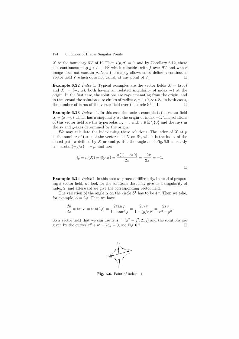
174 6 Indices of Planar Singular Points
X to the boundary ∂V of V . Then i(p, σ) = 0, and by Corollary 6.12, thereis a continuous map g : V → R2 which coincides with f over ∂V and whoseimage does not contain p. Now the map g allows us to define a continuousvector field Y which does not vanish at any point of V . �
Example 6.22 Index 1. Typical examples are the vector fields X = (x, y)and X ′ = (−y, x), both having an isolated singularity of index +1 at theorigin. In the first case, the solutions are rays emanating from the origin, andin the second the solutions are circles of radius r, r ∈ (0,∞). So in both cases,the number of turns of the vector field over the circle S1 is 1. �
Example 6.23 Index −1. In this case the easiest example is the vector fieldX = (x,−y) which has a singularity at the origin of index −1. The solutionsof this vector field are the hyperbolas xy = c with c ∈ R \ {0} and the rays inthe x- and y-axes determined by the origin.
We may calculate the index using these solutions. The index of X at pis the number of turns of the vector field X on S1, which is the index of theclosed path σ defined by X around p. But the angle α of Fig. 6.6 is exactlyα = arctan(−y/x) = −ϕ, and now
ip = ip(X) = i(p, σ) =α(1) − α(0)
2π=
−2π
2π= −1.
�
Example 6.24 Index 2. In this case we proceed differently. Instead of propos-ing a vector field, we look for the solutions that may give us a singularity ofindex 2, and afterward we give the corresponding vector field.
The variation of the angle α on the circle S1 has to be 4π. Then we take,for example, α = 2ϕ. Then we have
dy
dx= tan α = tan(2ϕ) =
2 tan ϕ
1 − tan2 ϕ=
2y/x
1 − (y/x)2=
2xy
x2 − y2.
So a vector field that we can use is X = (x2 − y2, 2xy) and the solutions aregiven by the curves x2 + y2 + 2cy = 0; see Fig. 6.7. �
Fig. 6.6. Point of index −1
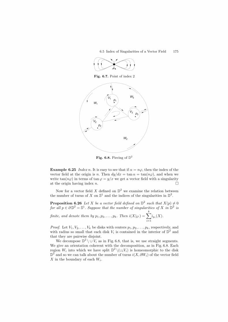
6.5 Index of Singularities of a Vector Field 175
Fig. 6.7. Point of index 2
p1
p3
p2
V1
V3
V2
W1
W3
W2
Fig. 6.8. Piecing of D2
Example 6.25 Index n. It is easy to see that if α = nϕ, then the index of thevector field at the origin is n. Then dy/dx = tan α = tan(nϕ), and when wewrite tan(nϕ) in terms of tan ϕ = y/x we get a vector field with a singularityat the origin having index n. �
Now for a vector field X defined on D2 we examine the relation between
the number of turns of X on S1 and the indices of the singularities in D2.
Proposition 6.26 Let X be a vector field defined on D2 such that X(p) �= 0
for all p ∈ ∂ D2 = S1. Suppose that the number of singularities of X in D
2 is
finite, and denote them by p1, p2, . . . , pk. Then i(X|S1) =
k∑
i=1
ipi(X).
Proof. Let V1, V2, . . . , Vk be disks with centers p1, p2, . . . , pk, respectively, andwith radius so small that each disk Vi is contained in the interior of D
2 andthat they are pairwise disjoint.
We decompose D2 \ ∪ Vi as in Fig. 6.8, that is, we use straight segments.
We give an orientation coherent with the decomposition, as in Fig. 6.8. Eachregion Wi into which we have split D
2 \(∪iVi) is homeomorphic to the diskD
2 and so we can talk about the number of turns i(X, ∂Wi) of the vector fieldX in the boundary of each Wi.
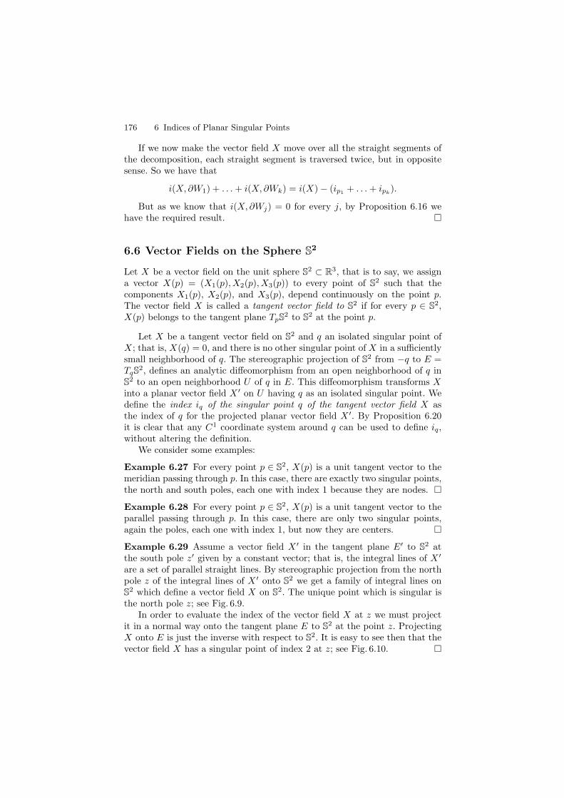
176 6 Indices of Planar Singular Points
If we now make the vector field X move over all the straight segments ofthe decomposition, each straight segment is traversed twice, but in oppositesense. So we have that
i(X, ∂W1) + . . . + i(X, ∂Wk) = i(X) − (ip1+ . . . + ipk
).
But as we know that i(X, ∂Wj) = 0 for every j, by Proposition 6.16 wehave the required result. �
6.6 Vector Fields on the Sphere S2
Let X be a vector field on the unit sphere S2 ⊂ R3, that is to say, we assigna vector X(p) = (X1(p), X2(p), X3(p)) to every point of S2 such that thecomponents X1(p), X2(p), and X3(p), depend continuously on the point p.The vector field X is called a tangent vector field to S2 if for every p ∈ S2,X(p) belongs to the tangent plane TpS2 to S2 at the point p.
Let X be a tangent vector field on S2 and q an isolated singular point ofX; that is, X(q) = 0, and there is no other singular point of X in a sufficientlysmall neighborhood of q. The stereographic projection of S2 from −q to E =TqS2, defines an analytic diffeomorphism from an open neighborhood of q inS2 to an open neighborhood U of q in E. This diffeomorphism transforms Xinto a planar vector field X ′ on U having q as an isolated singular point. Wedefine the index iq of the singular point q of the tangent vector field X asthe index of q for the projected planar vector field X ′. By Proposition 6.20it is clear that any C1 coordinate system around q can be used to define iq,without altering the definition.
We consider some examples:
Example 6.27 For every point p ∈ S2, X(p) is a unit tangent vector to themeridian passing through p. In this case, there are exactly two singular points,the north and south poles, each one with index 1 because they are nodes. �
Example 6.28 For every point p ∈ S2, X(p) is a unit tangent vector to theparallel passing through p. In this case, there are only two singular points,again the poles, each one with index 1, but now they are centers. �
Example 6.29 Assume a vector field X ′ in the tangent plane E′ to S2 atthe south pole z′ given by a constant vector; that is, the integral lines of X ′
are a set of parallel straight lines. By stereographic projection from the northpole z of the integral lines of X ′ onto S2 we get a family of integral lines onS2 which define a vector field X on S2. The unique point which is singular isthe north pole z; see Fig. 6.9.
In order to evaluate the index of the vector field X at z we must projectit in a normal way onto the tangent plane E to S2 at the point z. ProjectingX onto E is just the inverse with respect to S2. It is easy to see then that thevector field X has a singular point of index 2 at z; see Fig. 6.10. �
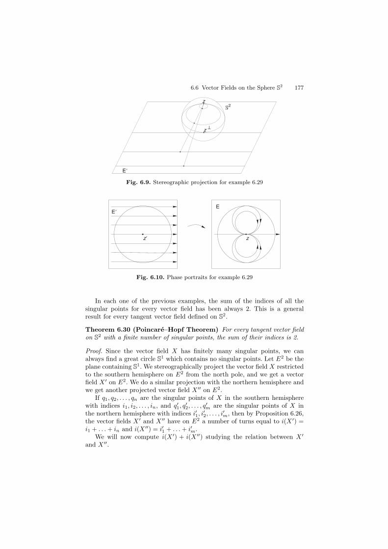
6.6 Vector Fields on the Sphere S2 177
z
E�
2
z ^
Fig. 6.9. Stereographic projection for example 6.29
zz�
EE�
Fig. 6.10. Phase portraits for example 6.29
In each one of the previous examples, the sum of the indices of all thesingular points for every vector field has been always 2. This is a generalresult for every tangent vector field defined on S2.
Theorem 6.30 (Poincare–Hopf Theorem) For every tangent vector fieldon S2 with a finite number of singular points, the sum of their indices is 2.
Proof. Since the vector field X has finitely many singular points, we canalways find a great circle S1 which contains no singular points. Let E2 be theplane containing S1. We stereographically project the vector field X restrictedto the southern hemisphere on E2 from the north pole, and we get a vectorfield X ′ on E2. We do a similar projection with the northern hemisphere andwe get another projected vector field X ′′ on E2.
If q1, q2, . . . , qn are the singular points of X in the southern hemispherewith indices i1, i2, . . . , in, and q′1, q
′2, . . . , q
′m are the singular points of X in
the northern hemisphere with indices i′1, i′2, . . . , i
′m, then by Proposition 6.26,
the vector fields X ′ and X ′′ have on E2 a number of turns equal to i(X ′) =i1 + . . . + in and i(X ′′) = i′1 + . . . + i′m.
We will now compute i(X ′) + i(X ′′) studying the relation between X ′
and X ′′.

178 6 Indices of Planar Singular Points
1
2πt 2πt+π/2
a(t )
a(0)
ϕ0
ϕ9
X 0
X 9
Fig. 6.11. The vector fields X ′ and X ′′ on D2
Let ϕ′ and ϕ′′ be the angle functions for X ′ and X ′′, respectively, over thepoints of S1. For each point a(t) ∈ S1 by construction the vector fields X ′ andX ′′ are symmetric with respect to the tangent line to S1 at a(t); see Fig. 6.11.
Thenϕ′(t) + ϕ′′(t)
2= 2πt + π/2,
consequentlyϕ′(t) + ϕ′′(t) = 4πt + π.
Therefore
i(X ′) + i(X ′′) =ϕ′(1) − ϕ′(0) + ϕ′′(1) − ϕ′′(0)
2π
=ϕ′(1) + ϕ′′(1) − (ϕ′(0) + ϕ′′(0))
2π
=4π + π − π
2π= 2,
and the result is proved. �
Corollary 6.31 Every tangent vector field X on S2 has singular points.
Proof. Considering any equator S1 ⊂ S2 and following the argumentationof the proof of Theorem 6.30, the absence of singular points implies thati(X ′) = i(X ′′) = 0. This contradicts the fact that i(X ′) + i(X ′′) = 2. �
The definition of index on the unit sphere S2 ⊂ R3 can be transferred toan “abstract” sphere, meaning any two-dimensional oriented surface diffeo-morphic to S2. As we have already observed, by Proposition 6.20, any localparametrization near the singular point can be used to calculate the index of avector field near an isolated singular point. In fact, the index does not change
6.7 Poincare Index Formula 179
even under a C0-equivalence. The notion of index can also be defined for anyC0 vector fields on an arbitrary compact oriented surface without boundary.
The Poincare–Hopf Theorem, as well as Corollary 6.31, clearly remain trueon an “abstract” sphere. A similar theorem (with a different proof), can beproved on an arbitrary compact oriented surface without boundary. Thus, ona compact oriented surface without boundary S, it can be proved that thesum of the indices of the vector field with finitely many singular points isequal to the Euler characteristic of S. This theorem was due to Poincare, andits extension to compact manifolds of arbitrary dimension is due to Hopf.
6.7 Poincare Index Formula
In Sect. 1.5 we have defined parabolic, hyperbolic, and elliptic sectors, and thefinite sectorial decomposition property for any isolated singular point differentfrom a center or a focus. By definition we say that a center and a focus haveneither elliptic, hyperbolic, nor parabolic sectors. It is easy to show that theindex of a focus, as well as the index of a center, is +1.
In order to study the index of any of the other singular points we have thefollowing result.
Proposition 6.32 (Poincare Index Formula) Let q be an isolated singu-lar point having the finite sectorial decomposition property. Let e, h, and pdenote the number of elliptic, hyperbolic, and parabolic sectors of q, respec-tively, and suppose that e + h + p > 0. Then iq = (e − h)/2 + 1.
Proof. Suppose that X is a continuous vector field defined in a neighborhoodV of q and suppose that X|V has the finite sectorial decomposition propertydefined in Sect. 1.5. If the sectorial decomposition is trivial, in the sense thatit consists of one parabolic sector, then iqX = 1 and (e, h) = (0, 0) whichclearly fits the statement. So we suppose that the decomposition is nontrivial,i.e., (e, h) �= (0, 0).
By definition ∂V is the image of a permissible parametrization, the vectorfield is nowhere tangent to ∂V except at e points s1, . . . , se where it has aninternal tangency (see Sect. 1.5) and h points r1, . . . , rh where it has an exter-nal tangency (see also Sect. 1.5). We can order these e + h contact points asq1, . . . , qn with n = e+h, using the cyclic order on ∂V , and choose intermedi-ate points pk ∈ (qk, qk+1) for k = 0, . . . , n − 1 and with q0 = qn. We can nowchoose a permissible parametrization ρ : S1 → ∂V such that ρ(e2πik/n) = pk.We suppose that X(p0) is pointing outward. By construction, n = e + his even and the vectors X(pk) are pointing outward for k even and inwardfor k odd.
Let N(e2πit) denote the exterior normal related to ρ. We can consider themapping
R : S1 × (−ε, ε) → R2
(e2πit, s) → ρ(e2πit) + sN(e2πit)
180 6 Indices of Planar Singular Points
which is a C1-diffeomorphism onto its image for ε > 0 sufficiently small. Wedefine the continuous vector field Y along S1 by
Y (e2πit, 0) = (dR(e2πit,0))−1(X(ρ(e2πit))).
Y along S1 is nothing else but X along ∂V written in different C1 coordinates.As such, i(X, ∂V ) = i(Y, S1).
Moreover, the tangency points of Y along S1 correspond to the tangencypoints of X along ∂V . We continue denoting them by q1, . . . , qn. We also writepk for e2πik/n. The vectors Y (pk) are hence pointing outward for k even andinward for k odd. Since it does not change the index i(Y, S1) we can sup-pose that Y |S1 consists of unit vectors, which can be achieved by consideringY (p)/‖Y (p)‖. We now fix neighborhoods (pk − ε, pk + ε) ⊂ S1, with ε > 0small enough such that they do not contain the tangency points q1, . . . , qn. Ineach Vk separately we can now easily deform the vector field Y , not chang-ing it at {pk − ε, pk + ε} and keeping it pointing outward on Vk for k evenand inward for k odd in such a way that, after deformation and still usingthe notation Y , Y (pk) = e2πik/n for k even and Y (pk) = −e2πik/n for kodd.
We can next deform the vector field Y on each [pk, pk+1] separately, chang-ing it into the field
Y (e2πit) = e2πi( kn
(1−s)+s( kπn
+π)) (6.1)
if there is a (unique) internal tangency in (pk, pk+1) and
Y (e2πit) = e2πi( kn
(1−s)+s( kπn
−π)) (6.2)
if there is a (unique) external tangency in (pk, pk+1).In both cases we use s = n(t − k/n) and the deformation can be taken
in such a way that the beginning and ending values Y (pk) and Y (pk+1) donot change. Thus, the different deformations on the respective [pk, pk+1] canbe joined to form a global deformation on S1. After this deformation we cansuppose that the vector field Y is exactly given by (6.1) (respectively (6.2))on the intervals [pk, pk+1] in which there is a (unique) internal (respectivelyexternal) tangency.
In short, by means of a continuous change, the index of a singular pointwith (e, h, p) sectors is equal to the index of a singular point with exactlythose same sectors, but each one of them being a triangular sector of an-gle 2π/m where m = e + h + p. Let σ be a circle of radius r with r smallenough.
We can now consider the contribution to the index of each sector.
(i) A triangular parabolic sector with angle 2π/m will start with an angleϕ(0) = α and will end with an angle ϕ(2π/m) = α + 2π/m, for a netgain of 2π/m.
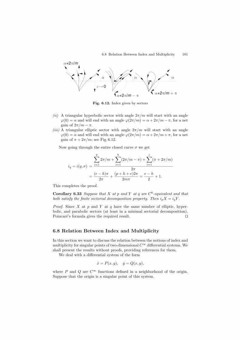
6.8 Relation Between Index and Multiplicity 181
α+2π/m
α+2π/m − πα+2π/m + π
ε→ 0
α α α
Fig. 6.12. Index given by sectors
(ii) A triangular hyperbolic sector with angle 2π/m will start with an angleϕ(0) = α and will end with an angle ϕ(2π/m) = α + 2π/m− π, for a netgain of 2π/m − π.
(iii) A triangular elliptic sector with angle 2π/m will start with an angleϕ(0) = α and will end with an angle ϕ(2π/m) = α + 2π/m + π, for a netgain of π + 2π/m; see Fig. 6.12.
Now going through the entire closed curve σ we get
iq = i(q, σ) =
p∑
i=1
2π/m +
h∑
i=1
(2π/m − π) +
e∑
i=1
(π + 2π/m)
2π
=(e − h)π
2π+
(p + h + e)2π
2mπ=
e − h
2+ 1.
This completes the proof.
Corollary 6.33 Suppose that X at p and Y at q are C0-equivalent and thatboth satisfy the finite sectorial decomposition property. Then ipX = iqY .
Proof. Since X at p and Y at q have the same number of elliptic, hyper-bolic, and parabolic sectors (at least in a minimal sectorial decomposition),Poincare’s formula gives the required result. ⊓⊔
6.8 Relation Between Index and Multiplicity
In this section we want to discuss the relation between the notions of index andmultiplicity for singular points of two-dimensional C∞ differential systems. Weshall present the results without proofs, providing references for them.
We deal with a differential system of the form
x = P (x, y), y = Q(x, y),
where P and Q are C∞ functions defined in a neighborhood of the origin.Suppose that the origin is a singular point of this system.
182 6 Indices of Planar Singular Points
Here, the germ (P0, Q0) of (P,Q) at 0 is the equivalence class of C∞
functions (F,G) defined in a neighborhood of 0 and equivalent to the function(P,Q) under the following equivalence relation. Two C∞ functions (F,G)and (P,Q) are equivalent if there is some open neighborhood U of 0 suchthat for all (x, y) ∈ U , the identity (F,G)(x, y) = (P,Q)(x, y) holds. All localproperties of (P,Q) at 0 depend only on its germ (P0, Q0).
We consider the germ (P0, Q0) of (P,Q) at 0, and the local ring given by
C∞0 (R2)/ < P0, Q0 >
of (P0, Q0) at 0, where C∞0 (R2) is the ring of germs at 0 of C∞ real-valued
functions on R2, and < P0, Q0 > is the ideal generated by P0 and Q0. Themultiplicity μ0[P,Q] of (P,Q) at 0 is defined by μ0[P,Q] = dimR[C∞
0 (R2)/ <P0, Q0 >] and we say that (P,Q) is a finite map germ if μ0[P,Q] < ∞. It isknown that μ0[P,Q] is the number of complex (P,Q)-preimages near 0 of aregular value of (P,Q) near 0. For more details and a proof of the followingstatements; see [4, 7].
Let (P,Q) : (R2, 0) → (R2, 0) be a finite map germ. Then the followingstatements hold.
(i) The multiplicity of (P,Q) at 0 does not depend on the chosen coordinates.(ii) Let P = Pk+ higher order terms and Q = Ql+ higher order terms, where
Pk (respectively Ql) denotes the homogeneous part of P (respectively Q)of degree k (respectively l). Then μ0[P,Q] ≥ kl, and μ0[P,Q] = kl if andonly if the system Pk = Ql = 0 only has the trivial solution (0, 0) in C2.
(iii) If P = P1P2, where P1(0) = P2(0) = 0, then μ0[P,Q] = μ0[P1, Q] +μ0[P2, Q]. A similar result holds for Q.
(iv) Let (F,G) : (R2, 0) → (R2, 0) also be a finite map germ. Then μ0[(P,Q)◦(F,G)] = μ0[P,Q]μ0[F,G].
(v) If G = Q + AP with A : (R2, 0) → R a C∞ function, then μ0[P,Q] =μ0[P,G]. A similar result holds for P .
(vi) If P = BF with B : (R2, 0) → R a C∞ function such that B(0) �= 0, thenμ0[P,Q] = μ0[F,Q]. A similar result holds for Q.
The next results, due to Eisenbud and Levine [60], show the relation be-tween index and multiplicity of a singular point of a two-dimensional differ-ential system.
Theorem 6.34 Let the origin be a singular point of the C∞ vector field X =(P,Q). Then the following two statements hold.
(i) |i0(X)| ≤√
μ0[X].(ii)i0(X) ≡ μ0[X] (mod 2).
The following natural question appears: Given the multiplicity μ = μ0[X],which values can the index i0(X) take? The next result due to Cima, Gasull,and Torregrosa [42] shows that the index i0(X) of a two-dimensional vectorfield is not subject to any restrictions other than the two conditions providedby Theorem 6.34.
6.10 Bibliographical Comments 183
Theorem 6.35 For each μ ∈ N with μ ≥ 1 and i ∈ Z satisfying |i| ≤ √μ and
i ≡ μ (mod 2), there exists a function germ X = (P,Q) : (R2, 0) → (R2, 0)such that i0(X) = i and μ0[X] = μ.
6.9 Exercises
Exercise 6.1 Prove the fundamental theorem of algebra. That is, let p(z) =zn + an−1z
n−1 + . . . + a1z + a0 be a polynomial with n ≥ 1 and ai ∈ C fori = 0, 1, . . . , n − 1. Then show that there exists z0 ∈ C such that p(z0) = 0.
Hint: Use Theorem 6.13 and Corollary 6.6.
Exercise 6.2 Let S2 = {x = (x1, x2, x3) ∈ R3 : x21 + x2
2 + x23 = 1}. A
continuous map f : S2 → R is odd, if for all x ∈ S2 we have that f(x) = −f(x).Prove the Borsuk’s Theorem: Two odd continuous maps f, g : S2 → R alwayshave a common zero.
Hint: Use Theorem 6.13.
Exercise 6.3 Prove the Brouwer Fixed Point Theorem: A continuous mapf : D
2 → D2 has at least one fixed point (i.e., there exists a point p ∈ D
2 suchthat f(p) = p).
Hint: Use Proposition 6.16 and Example 6.17.
Exercise 6.4 Let f : S2 → S2 be a continuous map. Show that f has apoint such that f(p) = p or f(p) = −p. Here S2 = {x = (x1, x2, x3) ∈ R3 :x2
1 + x22 + x2
3 = 1}.Hint: Use Corollary 6.31.
6.10 Bibliographical Comments
The authors have used in the preparation of this chapter some notes of M.Castellet from the University Autonoma de Barcelona.
For advanced versions of the Poincare–Hopf Theorem; see [85] and [111].For additional results on index theory in dimension 2; see [169].

7
Limit Cycles and Structural Stability
In the qualitative theory of differential equations, research on limit cyclesis an interesting and difficult topic. Limit cycles of planar vector fields weredefined in the famous paper Memoire sur les courbes definies par une equationdifferentielle [130,131]. At the end of the 1920s van der Pol [160], Lienard [99]and Andronov [3] proved that a periodic orbit of a self-sustained oscillationoccurring in a vacuum tube circuit was a limit cycle as considered by Poincare.After this observation, the existence and nonexistence, uniqueness, and otherproperties of limit cycles have been studied extensively by mathematicians andphysicists, and more recently also by chemists, biologists, and economists.
After singular points, limit cycles are the main subject of study in thetheory of two-dimensional differential systems. In this chapter we present themost basic results on limit cycles. In particular, we show that any topologicalconfiguration of a finite number of limit cycles is realizable by a suitablepolynomial differential system. We define the multiplicity of a limit cycle, andwe study the bifurcations of limit cycles for rotated families of vector fields.We present some results on structural stability.
7.1 Basic Results
We consider the system of differential equations
x =dx
dt= P (x, y), y =
dy
dt= Q(x, y), (7.1)
where x, y, and t are real variables, and P and Q are C1 functions of x andy. Then the existence and uniqueness of its solutions is guaranteed.
We recall that if a solution x = f(t), y = g(t) of system (7.1) is a noncon-stant periodic function of t, then γ = {(x, y) : x = f(t), y = g(t)} is called aperiodic orbit of system (7.1).
186 7 Limit Cycles and Structural Stability
If for some arbitrarily small outer (inner) neighborhood of the periodicorbit γ there do not exist other periodic orbits, then γ is called an externally(internally) limit cycle.
If there is an arbitrarily small outer (inner) neighborhood of the periodicorbit γ filled with periodic orbits, then γ is called an externally (internally)center-type periodic orbit. Sometimes in the literature this is simply calledan externally (internally) periodic orbit, omitting “center-type.” We prefer toadd center-type to avoid confusion.
If in any outer (inner) neighborhood of the periodic orbit γ there existboth nonperiodic and periodic orbits different from γ, then γ is called anexternally (internally) indefinite cycle. If a periodic orbit is either externallyor internally indefinite we call it an indefinite cycle. In the literature one canalso find “compound” instead of “indefinite,” but since “compound cycle”means something completely different in [6] we prefer to use “indefinite.”Sometimes one can even find the word “compound limit cycles,” although onat least one side no regular orbits tend to them, either in positive or negativetime.
By the Poincare–Bendixson Theorem, the following three propositions andthe first theorem hold.
Proposition 7.1 If γ is a periodic orbit of system (7.1) then there existsa sufficiently small neighborhood U of γ satisfying the following three state-ments.
(i) U does not contain singular points.(ii) Through any point p ∈ γ there exists a sufficiently small transverse seg-
ment Σp for the flow of system (7.1); that is, the vector field associatedto system (7.1) at the points of Σp is not tangent to it.
(iii) Any periodic orbit in U intersects Σp transversely at a unique point. Anynonperiodic orbit in U intersects Σp at an infinite number of points, whichlie on the same side of γ.
Proposition 7.2 Any periodic orbit γ is either an external (internal) limitcycle, an external (internal) center-type periodic orbit or an external (inter-nal) indefinite cycle. The first case can be divided into the following two sub-cases:
(i) There exists a sufficiently small outer (inner) neighborhood of γ such thatall the orbits in it are nonperiodic, and they have γ as ω-limit set. Then γis called an externally (internally) stable limit cycle. If γ is externally andinternally stable, then we say that γ is a stable limit cycle.
(ii)There exists a sufficiently small outer (inner) neighborhood of γ such thatall the orbits in it are nonperiodic, and they have γ as their α-limit set.Then γ is called an externally (internally) unstable limit cycle. If γ isexternally and internally unstable, then we say that γ is an unstable limitcycle.

7.1 Basic Results 187
If γ is externally stable and internally unstable or the opposite, then wesay that γ is a semistable limit cycle.
Proposition 7.3 If γ1 and γ2 are periodic orbits which form the boundaryof an annular region A, and there are neither singular points nor other pe-riodic orbits in A, then all the orbits in A have γ1 as their ω-limit set andγ2 as their α-limit set, or conversely. In other words, two adjacent periodicorbits (under the above conditions) possess different stability on the adjacentsides.
Theorem 7.4 (Poincare’s Annular Region Theorem) Let A be an an-nular region not containing singular points such that ∂A does not containperiodic orbits and such that every orbit crossing the boundary of A movesfrom the exterior to the interior (interior to the exterior). Then there existsat least one externally stable (unstable) limit cycle in A, and there exists atleast one internally stable (unstable) limit cycle in A; it is possible that bothlimit cycles coincide, so as to be a single stable (unstable) limit cycle.
For analytic systems some restrictions occur in the classification of periodicorbits.
Proposition 7.5 If P and Q are analytic functions, then system (7.1) hasno indefinite limit cycles.
The proof easily follows from Propositions 7.1 and 7.2, observing that thePoincare map on Σp is analytic, if we chose Σp to be an analytic regular arcwith an analytic and regular parameter. For polynomial systems (7.1) thereis a famous result, whose complicated proof has been given independently byEcalle [59] and Il’yashenko [88].
Theorem 7.6 When P and Q are polynomials then system (7.1) has at mostfinitely many limit cycles.
The proof of the next result is straightforward.
Proposition 7.7 (Symmetry Principle) Suppose that in equations (7.1)
P (x, y) = P (−x, y), Q(−x, y) = −Q(x, y),
and the origin is the only singular point on the y-axis. If a trajectory γ startsfrom the positive y-axis and returns to the negative y-axis, then γ is a periodicorbit. If all the trajectories near the origin have this property, then the originis a center.
Using the Intermediate Value Theorem the next result is easy to prove.
Proposition 7.8 If the Poincare map determined by the trajectory carriessome closed segment into itself, then the equations must have a periodic orbit.
188 7 Limit Cycles and Structural Stability
Proposition 7.9 (Poincare Method of Tangential Curves) Consider afamily of curves F (x, y) = C, where F (x, y) is cont inuously differentiable. Ifin a region R the quantity
dF
dt=
∂F
∂x
dx
dt+
∂F
∂y
dy
dt= P
∂F
∂x+ Q
∂F
∂y
(which represents the rate of change of the function F with respect to t alonga trajectory of system (7.1)) has constant sign, and the curve
P∂F
∂x+ Q
∂F
∂y= 0
(which represents the locus of points of contact between curves in the familyand the trajectories of (7.1), and is called a tangential curve) does not containa whole trajectory of (7.1) or any closed branch, then system (7.1) does notpossess a periodic orbit which is entirely contained in R.
Proof. Suppose the hypotheses hold, but system (7.1) has a periodic orbit Γthat is wholly contained in R. If we integrate P∂F/∂x + Q∂F/∂y along Γ inthe direction of increasing t, we obtain
∫
Γ
(P∂F
∂x+ Q
∂F
∂y)dt =
∫
Γ
dF
dtdt.
Since Γ is periodic, we know that the right side of the equation above isequal to zero; however, on the other hand, the integrand on the left of thisequality has a constant sign, but is not identically zero on Γ , and t monotoni-cally increases along Γ ; hence its value is different from zero, a contradiction.
�
Theorem 7.10 (Bendixson’s Theorem) Assume that the divergence func-tion ∂P/∂x + ∂Q/∂y of system (7.1) has constant sign in a simply connectedregion R, and is not identically zero on any subregion of R. Then system (7.1)does not have a periodic orbit which lies entirely in R. (We assume that Pand Q are C1.)
Proof. Suppose the hypotheses hold, but system (7.1) has a closed trajectoryΓ . Since R is simply connected, Γ and its interior S lie entirely in R. FromGreen’s formula we have
∫
Γ
Pdy − Qdx =
∫∫
S
(∂P
∂x+
∂Q
∂y
)dxdy. (7.2)
But Pdy −Qdx = 0 holds everywhere along Γ , since Γ is an orbit. Hence theleft side of (7.2) is zero, while the integrand on the right side has constant signbut is not identically zero in S; hence the double integral is not zero, givinga contradiction. �

7.1 Basic Results 189
Remark 7.11 By the same arguments as in Theorem 7.10, i.e., the use ofGreen’s formula, it follows that on any region bounded by periodic orbits, theintegral of the divergence, as defined in (7.2) is equal to zero.
Theorem 7.12 (Dulac’s Theorem) If there exists a C1 function B(x, y)in a simply connected region R such that ∂(BP )/∂x+∂(BQ)/∂y has constantsign and is not identically zero in any subregion, then system (7.1) does nothave a periodic orbit lying entirely in R. (We assume that P and Q are C1.)
Proof. We follow the proof of Theorem 7.10 but use BP and BQ in place ofP and Q, respectively. �
We shall call B(x, y) a Dulac function, and the method of proving the non–existence of a periodic orbit, as given in Theorem 7.10, is called the methodof Dulac functions.
Theorems 7.10 and 7.12 can be generalized as follows.
Theorem 7.13 (Generalized Dulac’s Theorem) If we change the regionR in Bendixson’s Theorem or in Dulac’s Theorem to be n-multiply connected(i.e., R has one or several outer boundary curves, and n − 1 inner boundarycurves), then system (7.1) has at most n− 1 periodic orbits which lie entirelyin R.
Proof. From the proof of Theorem 7.10 we know that if there is a closedtrajectory Γ of system (7.1) in R, then Γ should contain at least one innerboundary curve C of R in its interior. Similarly, we also know that if theinterior of Γ also contains other closed trajectories Γ1, . . . , Γk, then the regionin the interior of Γ but in the exterior of all the trajectories Γ1, . . . , Γk alsocontains at least one inner boundary curve C, because of Remark 7.11. We saythat C corresponds to Γ ; we can see that for different Γ their correspondingcurves C are also different. Hence if the number of closed trajectories in G ismore than n− 1, then the connectivity number of G must be greater than n.The theorem is proved. �
Proposition 7.14 If P and Q of system (7.1) are C1 on an open subsetU ⊂ R2, and ∂P/∂x + ∂Q/∂y ≡ 0, i.e., the 1-form
Pdy − Qdx (7.3)
is closed, then (7.1) does not have indefinite cycles in U , nor limit cycles norone-sided limit cycles in R.
Proof. Suppose that U contains a closed orbit Γ of system X, expressed by(7.1) and consider a transverse section Σ consisting of a piece of orbit of thevector field P∂/∂y−Q∂/∂x, orthogonal to X. Consider now an open segmentΣ0 ⊂ Σ, containing Σ ∩ Γ , on which a Poincare map P : Σ0 → Σ is defined.Take any p ∈ Σ0 \Γ , let q = P (p) and denote by A ⊂ U the annulus boundedby Γ ∪γpq ∪Σpq where γpq is the piece of X-orbit between p and q, and Σpq is
190 7 Limit Cycles and Structural Stability
the segment in Σ between p and q. Since the divergence of X is equal to zero,it follows from Green’s formula (7.2) on A that necessarily p = q (we leavethe details of the elaboration as an exercise). Hence all orbits in U sufficientlyclose to Γ have to be closed, proving our claim. �
Let U be an open subset of R2. In this book we consider only C1 mapsV defined in U such that the set {(x, y) ∈ U : V (x, y) = 0} is locally a onedimensional manifold except perhaps at finitely many points.
Let (P,Q) be a C1 vector field defined in U . A standard method for deter-mining an explicit solution of the vector field (P,Q) is to find a C1 solutionV = V (x, y) of the linear partial differential equation
P∂V
∂x+ Q
∂V
∂y= RV, (x, y) ∈ U, (7.4)
for some C1 map R = R(x, y). Thus the curve V (x, y) = 0 is formed by tra-jectories of the vector field (P,Q), because (7.4) shows that (P,Q) is tangentto the curve V (x, y) = 0.
In the next two results we use equation (7.4) to study the periodic solutionsof the vector field (P,Q). Both results are proved in [72].
Theorem 7.15 Let (P,Q) be a C1 vector field defined on the open subset Uof R2, let (u(t), v(t)) be a periodic solution of (P,Q) of period T , R : U → R
a C1 map such that∫ T
oR(u(t), v(t)) dt �= 0, and V = V (x, y) a C1 solution
of the linear partial differential equation (7.4). Then the closed trajectory γ ={(u(t), v(t)) ∈ U : t ∈ [0, T ]} is contained in Σ = {(x, y) ∈ U : V (x, y) = 0},and γ is not contained in a period annulus of (P,Q). Moreover, if the vectorfield (P,Q) and the functions R and V are analytic, then γ is a limit cycle.
We introduce a few new notions. We consider the C1 vector field
X = P∂
∂x+ Q
∂
∂y
defined on the open subset U of R2. Then X is a closed vector field on U if
∂P
∂x= −∂Q
∂y,
for all (x, y) ∈ U . Furthermore, if U is simply connected, then there exists afunction H : U → R satisfying
P = −∂H
∂y, Q =
∂H
∂x.
The function H is the Hamiltonian of the Hamiltonian vector field X. Clearlythe Hamiltonian function is a first integral of X.
7.1 Basic Results 191
A C1 function R : U → R such that
∂(RP )
∂x= −∂(RQ)
∂y(7.5)
is an integrating factor of the vector field X. We know that R is an integratingfactor of X in U if and only if R is a solution of the partial differential equation
P∂R
∂x+ Q
∂R
∂y= −
(∂P
∂x+
∂Q
∂y
)R (7.6)
in U .A function V : U → R is an inverse integrating factor of the vector field
X if V verifies the partial differential equation
P∂V
∂x+ Q
∂V
∂y=
(∂P
∂x+
∂Q
∂y
)V (7.7)
in U . We note that V satisfies (7.7) in U if and only if R = 1/V satisfies (7.6)in U \ {(x, y) ∈ U : V (x, y) = 0}.
Here we provide an easier and direct proof of the next theorem from [72].
Theorem 7.16 Let X be a C1 vector field defined on the open subset U ofR2. Let V : U → R be an inverse integrating factor of X. If γ is an indefinitecycle, a limit cycle or an one-sided limit cycle of X, then γ is contained inS = {(x, y) ∈ U : V (x, y) = 0}.
Proof. Due to the existence of the inverse integrating factor V defined on U ,we see that the vector field X/V is Hamiltonian in U \S, hence its divergenceis identically zero. The result now follows from Proposition 7.14. �
Example 7.17 The system
x = λx − y + λm1x3 + (m2 − m1 + m1m2)x
2y + λm1m2xy2 + m2y3,
y = x + λy − x3 + λm1x2y + (m1m2 − m1 − 1)xy2 + λm1m2y
3,(7.8)
has the following inverse integrating factor
V (x, y) = (x2 + y2)(1 − m1x2 + m1m2y
2).
Since V is defined in the whole plane, by Theorem 7.16 follows that (7.8)has at most one limit cycle, and when it exists it is algebraic and has theequation
1 − m1x2 + m1m2y
2 = 0. (7.9)
Note that such a limit cycle exists if and only if system (7.8) has no singularpoints on the curve (7.9).
192 7 Limit Cycles and Structural Stability
7.2 Configuration of Limit Cycles and AlgebraicLimit Cycles
By Theorem 7.6, a theorem proved independently by Ecalle [59] and byIl’yashenko [88], we know that a polynomial planar system (7.1) can onlyhave a finite number of limit cycles. It is not known, however, not even forquadratic systems, whether there exists a uniform upper bound, dependingon the degree of the system. This is an old question, put forward by Hilbertin 1900 [82] as part of the 16th problem in his famous list of “problems forthe 20th–century.” Besides asking for such a uniform upper bound, Hilbert’s16th problem, or more precisely the second part of it (the first part dealingwith ovals in a zero set of algebraic functions), also asks for a descriptionof the possible configurations of limit cycles which polynomial systems canhave.
We now deal with this problem, presenting the results obtained in [102].A configuration of closed curves is a finite set C = {C1, . . . , Cn} of disjoint
simple closed curves of the plane such that Ci ∩ Cj = ∅ for all i �= j. We callit a configuration of limit cycles if the closed curves Ci are limit cycles, anda configuration of algebraic limit cycles if the closed curves Ci are algebraiclimit cycles. A closed curve is called algebraic if it is a connected componentof the zero set of some polynomial function.
Given a configuration of closed curves C = {C1, . . . , Cn} the curve Ci isa primary curve if there is no curve Cj of C contained in the bounded regiondetermined by Ci.
Two configurations of closed curves C = {C1, . . . , Cn} and C ′ = {C ′1, . . .,
C ′m} are (topologically) equivalent if there is a homeomorphism h : R2 → R2
such that h (∪ni=1Ci) = (∪m
i=1C′i). Of course, for equivalent configurations of
closed curves C and C ′ we have that n = m.We say that the vector field X realizes the configuration of closed curves C
as a configuration of limit cycles if the set of all limit cycles of X is equivalentto C.
Theorem 7.18 Let C = {C1, . . . , Cn} be a configuration of closed curves,and let r be the number of its primary curves. Then the following statementshold.
(i) The configuration C is realizable as a configuration of limit cycles by apolynomial vector field.
(ii)The configuration C is realizable as a configuration of algebraic limit cyclesby a polynomial vector field of degree ≤ 2(n + r) − 1.
In the proof of this theorem we provide an explicit expression for thepolynomial differential system of degree at most 2(n + r)− 1 satisfying state-ment (ii) of Theorem 7.18. Of course, statement (i) of Theorem 7.18 followsimmediately from statement (ii).

7.2 Configuration of Limit Cycles and Algebraic Limit Cycles 193
Proof. Let C = {C1, . . . , Cn} be the configuration of closed curves given in thestatement of Theorem 7.18. For every primary curve Cj we select a point pj inthe interior of the bounded component determined by Cj . Since we can workwith an equivalent configuration of limit cycles, without loss of generality, wecan assume that
(i) each curve Ci is a circle defined by
fi(x, y) = (x − xi)2 + (y − yi)
2 − r2i = 0,
for i = 1, . . . , n; and that(ii)the primary curves of the configuration C are the curves Cj , and the
selected points pj have coordinates (xj , yj), for j = 1, . . . , r.
For every selected point pj we define
fn+2j−1(x, y) = (x − xj) + i(y − yj),
fn+2j(x, y) = (x − xj) − i(y − yj).
Now we consider the function
H = fλ1
1 · · · fλnn f
λn+1
n+1 fλn+2
n+2 · · · fλn+2r−1
n+2r−1 fλn+2r
n+2r =n+2r∏
k=1
fλk
k ,
with λ1 = · · · = λn = 1, and λn+2j−1 = 1 + i and λn+2j = 1 − i, forj = 1, . . . , r. After an easy computation, we see that
H(x, y) = A(x, y)B(x, y)C(x, y),
where
A(x, y) =n∏
i=1
[(x − xi)
2 + (y − yi)2 − r2
i
],
B(x, y) =
r∏
j=1
[(x − xj)
2 + (y − yj)2],
C(x, y) = exp
⎛⎝−2
r∑
j=1
arg[(x − xj) + i (y − yj)]
⎞⎠.
Clearly H(x, y) is a real function. Therefore, the function
H = log H =
n+2r∑
k=1
λk log fk
is also real.
194 7 Limit Cycles and Structural Stability
We claim that the vector field
X = P (x, y)∂
∂x+ Q(x, y)
∂
∂y
= −n+2r∑
k=1
λk
⎛⎜⎝
n+2r∏
l=1l =k
fl
⎞⎟⎠ ∂fk
∂y
∂
∂x+
n+2r∑
k=1
λk
⎛⎜⎝
n+2r∏
l=1l =k
fl
⎞⎟⎠ ∂fk
∂x
∂
∂y,
satisfies the conclusion of statement (ii) of Theorem 7.18. Now we shall provethe claim.
First, we note that we have the equalities
∂H
∂x=
Qn+2r∏
k=1
fk
,∂H
∂y= − P
n+2r∏
k=1
fk
. (7.10)
Therefore, since H and∏n+2r
k=1 fk are real functions, we get that P , Q, andconsequently X are real.
Clearly from the definition of X it follows that P and Q are polynomialsof degree at most n + 2r − 1. So X is a real polynomial vector field of degreeat most n + 2r − 1.
From (7.10) it follows that V =∏n+2r
k=1 fk is a polynomial inverse integrat-ing factor of X, and that H is a Hamiltonian for the Hamiltonian vector field
1
VX =
P
V
∂
∂x+
Q
V
∂
∂y,
defined on R2 \ {V = 0}.Since V is polynomial, V is defined on all of R2. Therefore, by Theorem
7.16 and since V (x, y) = 0 if and only if (x, y) ∈ (∪ni=1Ci)∪{p1, . . . , pr}, if the
vector field X has limit cycles, these must be the circles Ci for i = 1, . . . , n.Now we shall prove that all these circles are limit cycles. Hence the polynomialvector field X will realize the configuration of limit cycles {C1, . . . , Cn} andthe theorem will be proved.
We note that since H = exp(H) is a first integral of the vector field X onR2 \ {V = 0}, the circles are formed by solutions because they are containedin the level curve V = 0, where V is the associated inverse integrating factorof the Hamiltonian H, and V = 0 is formed by solutions. Now we shall provethat on every circle Ci there are no singular points of X, hence Ci will be aperiodic orbit. Assume to the contrary that (x0, y0) is a singular point of X onthe circle Ci; i.e., P (x0, y0) = Q(x0, y0) = fi(x0, y0) = 0. From the definitionof P and Q we have that
P (x0, y0) = −λi
⎛⎜⎝
n+2r∏
l=1l =i
fl(x0, y0)
⎞⎟⎠ ∂fi
∂y(x0, y0) = 0,

7.3 Multiplicity and Stability of Limit Cycles 195
Q(x0, y0) = λi
⎛⎜⎝
n+2r∏
l=1l =i
fl(x0, y0)
⎞⎟⎠ ∂fi
∂x(x0, y0) = 0.
Since fl(x0, y0) �= 0 for l �= i, we obtain that ∂fi
∂x (x0, y0) = 0 and also that∂fi
∂y (x0, y0) = 0. Therefore the point (x0, y0) is the center of the circle Ci,
contradicting the fact that fi(x0, y0) = 0. Hence every circle Ci is a periodicorbit of the vector field X. Now we shall prove that Ci is a limit cycle, andthis will complete the proof of Theorem 7.18.
We note that all circles Ci and all points pj are in the level H(x, y) = 0,and that they are the unique orbits of X at this level. Now suppose that Ci
is not a limit cycle. Then there is a periodic orbit γ = {(x(t), y(t)) : t ∈ R}different from C1, . . . , Cn and so close to Ci such that in the bounded com-ponent B determined by γ there are the same points of {p1, . . . , pr} as inthe bounded component determined by Ci. Without loss of generality we canassume that these points are p1, . . . , ps.
As γ is different from C1, . . . , Cn, there exists h �= 0 such that
H(x(t), y(t)) = A(x(t), y(t))B(x(t), y(t)) exp
⎛⎝−2
r∑
j=1
θj(t)
⎞⎠ = h, (7.11)
where θj(t) = arg[(x(t) − xj) + i (y(t) − yj)]. The function A(x(t), y(t))B(x(t), y(t)) is bounded on γ. Clearly the angles θ1(t), . . . , θs(t) all tend si-multaneously (due to the definition) to either +∞ or −∞ as t → +∞, whilethe angles θs+1(t), . . . , θr(t) remain bounded when t → +∞. These facts arein contradiction to equality (7.11). Consequently, we have proved that Ci is alimit cycle. In short, Theorem 7.18 is proved. �
7.3 Multiplicity and Stability of Limit Cycles
We have already defined the stability of limit cycles for a system of equations(7.1). In applications only a stable limit cycle has practical significance, sinceevery spiral sufficiently close to a limit cycle can approximately representthe limit cycle independent of initial conditions, and an unstable limit cycleis similar to an unstable equilibrium position in mechanics, which in realitycannot be seen. Hence the problem of distinguishing stability of limit cyclesbecomes a very important one.
From Sect. 1.6 we know that if along a closed trajectory γ of system (7.1)
∫ T
0
(∂P
∂x+
∂Q
∂y
)dt < 0 (respectively > 0), (7.12)
196 7 Limit Cycles and Structural Stability
then γ is a stable (respectively unstable) limit cycle. From this result it followsthat for all other periodic orbits, we must have
∫ T
0
(∂P
∂x+
∂Q
∂y
)dt = 0. (7.13)
However, when γ is an ordinary stable or unstable limit cycle (7.13) may alsohold since (7.12) is only a sufficient condition, not a necessary condition.
When condition (7.12) holds, we say that γ is a hyperbolic limit cycle;when condition (7.13) holds, we say that γ is a multiple periodic orbit, calleda multiple limit cycle if it is a limit cycle, both externally and internally.
Let Σ be a transverse segment (parametrized by s) to the flow of (7.1)and let p(s) be the Poincare map over Σ. We define by d(s) = p(s) − s theso called displacement function. We clearly have the following result, whoseproof we leave as an exercise.
Theorem 7.19 If, for a given closed trajectory γ,
d′(0) = d′′(0) = . . . = d(k−1)(0) = 0 and d(k)(0) < 0 (respectively > 0),(7.14)
for k odd, then γ is a stable (respectively unstable) limit cycle. If
d′(0) = d′′(0) = . . . = d(k−1)(0) = 0 and d(k)(0) �= 0, (7.15)
for k even, then γ is a semistable limit cycle.
Any γ satisfying condition (7.14) or (7.15) is called a k-multiple limit cycle.
7.4 Rotated Vector Fields
Consider the system of differential equations
dx
dt= P (x, y, α),
dy
dt= Q(x, y, α), (7.16)
with parameter α. Until now we have not yet considered how an orbit orhow the phase portrait changes as a parameter α varies. Such problems areinteresting but can also be very complicated. Suppose that as the parameterα is perturbed slightly near α0, the topological structure of the phase por-trait of (7.16)α0
is unchanged; then α0 is called a regular value of α, and thesystem (7.16)α0
is called structurally stable with respect to perturbations of α.If for arbitrarily small perturbations α near α0, the topological structure ofthe phase portrait for system (7.16)α is changed, then we say that α0 is abifurcation value and the change in topological structure is called a bifurca-tion. For example, as the parameter α changes, a limit cycle may appear ordisappear near a singular point, or one limit cycle may split into several ones;

7.4 Rotated Vector Fields 197
these are called bifurcation phenomena. Bifurcation theory is an active areain differential equations; the reader is referred to [35].
In this section, we concentrate on the dependence of limit cycles on theparameter α. The changes are very complicated for general 1-parameter fami-lies; hence, we will restrict our attention to a special situation: rotated vectorfields. The method of rotated vector fields is important in the sense that itprovides tractable 1-parameter families of polynomial vector fields of a fixeddegree, although it is definitely useful in a much more general context. Wediscuss the changes of limit cycles in rotated planar vector fields as the pa-rameter varies. That is, we study the appearance and disappearance of limitcycles as the parameter varies. In the special situation under consideration,the changes are very systematic.
In this section we assume that the vector field (7.16) has only isolatedsingular points, and that P (x, y, α) and Q(x, y, α) are C1 functions on R× I,where I : 0 ≤ α ≤ T or −∞ < α < +∞ and R ⊂ R2 is an open region.
Suppose that, as α varies in [0, T ], the singular points of the vector field(7.16) are unchanged, and at all the regular points
∣∣∣∣∣P Q∂P
∂α
∂Q
∂α
∣∣∣∣∣ > 0; (7.17)
moreover
P (x, y, α + T ) = − P (x, y, α),
Q(x, y, α + T ) = − Q(x, y, α).(7.18)
Then (7.16) is said to form a complete family of rotated vector fields, for0 ≤ α ≤ T .
From (7.18), it follows that P (x, y, α) and Q(x, y, α) can be extended asperiodic functions of α with period 2T .
Let θ be the angle between the vector field (P,Q) and the x-axis; then wehave
∂θ
∂α=
∂
∂αArctan
Q
P=
1
P 2 + Q2
∣∣∣∣∣P Q∂P
∂α
∂Q
∂α
∣∣∣∣∣ .
From condition (7.17), it follows that at all regular points p = (x, y), whenthe parameter α increases, the vector field (7.16) rotates counter-clockwise atthe point p. From condition (7.18), when the parameter changes from α toα + T , the vector (P,Q) rotates exactly π radians counter-clockwise at thepoint p, and the length of the vector remains the same. Thus, when α changesto α + 2T , the vector field (P,Q) rotates 2π radians counter-clockwise to itsoriginal position. This is the geometric meaning of “rotation and complete”in Duff’s definition; see for more details [50]. As the parameter α varies, thechange on limit cycles in rotated vector fields is relatively systematic; however,the restrictions in the definition of complete family of rotated vector fields arequite strong. These restrictions can be substantially reduced if we retain only
198 7 Limit Cycles and Structural Stability
the fundamental requirements. For example, Chen Xiang–Yan introduced gen-eralized rotated vector fields, where limit cycles vary in the same systematicway as the parameter varies; see [165–167]. This will be our approach.
Suppose that as α varies in (a, b), the singular points of the vector fields(7.16) remain unchanged, and for any given point p = (x, y) and any parame-ters α1 < α2 in (a, b), we have
∣∣∣∣P (x, y, α1) Q(x, y, α1)P (x, y, α2) Q(x, y, α2)
∣∣∣∣ ≥ 0 (or ≤ 0), (7.19)
where equality cannot hold on an entire periodic orbit of (7.16)αi, i = 1, 2.
Then (7.16) are called generalized rotated vector fields. Here, the interval (a, b)can be either bounded or unbounded.
If for a regular point (x0, y0) and parameter α0, there exists δ(x0, y0, α0)positive such that for all α ∈ [α0 − δ, α0 + δ], equality holds in (7.19), then α0
is called a stopping point for (x0, y0); otherwise, α0 is called a rotating point.Stopping points are allowed in generalized rotated vector fields. Moreover,generalized rotated vector fields do not necessarily depend on α periodically;in particular, condition (7.18) is not required.
The geometric meaning of condition (7.19) is that, at any point p =(x, y), the oriented angle between (P (x, y, α1), Q(x, y, α1)) and (P (x, y, α2),Q(x, y, α2)) has the same (or opposite) sign as sgn(α2 − α1). That is, atany point p = (x, y), as the parameter α increases, the vector (P (x, y, α),Q(x, y, α)) can only rotate in one direction; moreover, the angle of rotationcannot exceed π.
In the following, we describe two examples of rotated vector fields.
Example 7.20 Consider the system of differential equations
dx
dt= P (x, y),
dy
dt= Q(x, y)
where P,Q are of class C1. Consider the system of differential equations con-taining parameter α
dx
dt= P cos α − Q sin α,
dy
dt= P sin α + Q cos α. (7.20)
It is not difficult to verify that equations (7.20) satisfy conditions (7.17)and (7.18) and thus form a complete family of rotated vector fields. In 0 < α ≤π (7.20) represents generalized rotated vector fields, but not in 0 < α ≤ 2π.We remark that (7.20) is analytic when P and Q are, while the vector fields in(7.20) are all polynomial of degree n if (P,Q) represents a polynomial vectorfield of degree n.
In fact (7.20) can be regarded as a formula for axis rotation. It rotates theoriginal vector field by an angle of α, and keeps the vector lengths unchanged.Thus (7.20) are called uniformly rotated vector fields.
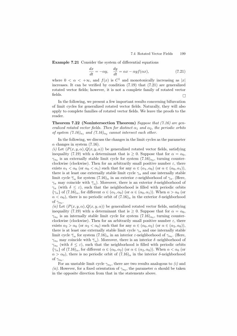
7.4 Rotated Vector Fields 199
Example 7.21 Consider the system of differential equations
dx
dt= −αy,
dy
dt= αx − αyf(αx), (7.21)
where 0 < α < +∞, and f(x) is C1 and monotonically increasing as |x|increases. It can be verified by condition (7.19) that (7.21) are generalizedrotated vector fields; however, it is not a complete family of rotated vectorfields.
In the following, we present a few important results concerning bifurcationof limit cycles for generalized rotated vector fields. Naturally, they will alsoapply to complete families of rotated vector fields. We leave the proofs to thereader.
Theorem 7.22 (Nonintersection Theorem) Suppose that (7.16) are gen-eralized rotated vector fields. Then for distinct α1 and α2, the periodic orbitsof system (7.16)α1
and (7.16)α2cannot intersect each other.
In the following, we discuss the changes in the limit cycles as the parameterα changes in system (7.16).(i) Let (P (x, y, α), Q(x, y, α)) be generalized rotated vector fields, satisfyinginequality (7.19) with a determinant that is ≥ 0. Suppose that for α = α0,γα0
is an externally stable limit cycle for system (7.16)α0, turning counter-
clockwise (clockwise). Then for an arbitrarily small positive number ε, thereexists α1 < α0 (or α0 < α1) such that for any α ∈ (α1, α0) (or α ∈ (α0, α1)),there is at least one externally stable limit cycle γα and one internally stablelimit cycle γα for system (7.16)α in an exterior ε-neighborhood of γα. (Here,γα may coincide with γα). Moreover, there is an exterior δ-neighborhood ofγα (with δ ≤ ε), such that the neighborhood is filled with periodic orbits{γα} of (7.16)α, for different α ∈ (α1, α0) (or α ∈ (α0, α1)). When α > α0 (orα < α0), there is no periodic orbit of (7.16)α in the exterior δ-neighborhoodof γα0
.(ii) Let (P (x, y, α), Q(x, y, α)) be generalized rotated vector fields, satisfyinginequality (7.19) with a determinant that is ≥ 0. Suppose that for α = α0,γα0
is an internally stable limit cycle for system (7.16)α0, turning counter-
clockwise (clockwise). Then for an arbitrarily small positive number ε, thereexists α2 > α0 (or α2 < α0) such that for any α ∈ (α0, α2) (or α ∈ (α2, α0)),there is at least one externally stable limit cycle γα and one internally stablelimit cycle γα for system (7.16)α in an interior ε-neighborhood of γα0
. (Here,γα0
may coincide with γα). Moreover, there is an interior δ–neighborhood ofγα0
(with δ ≤ ε), such that the neighborhood is filled with periodic orbits{γα} of (7.16)α, for different α ∈ (α0, α2) (or α ∈ (α2, α0)). When α < α0 (orα > α0), there is no periodic orbit of (7.16)α in the interior δ-neighborhoodof γα0
.For an unstable limit cycle γα0
, there are two results analogous to (i) and(ii). However, for a fixed orientation of γα0
, the parameter α should be takenin the opposite direction from that in the statements above.
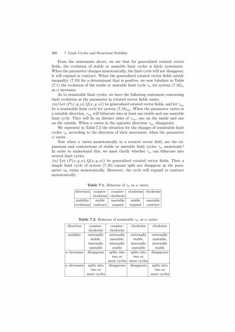
200 7 Limit Cycles and Structural Stability
From the statements above, we see that for generalized rotated vectorfields, the evolution of stable or unstable limit cycles is fairly systematic.When the parameter changes monotonically, the limit cycle will not disappear;it will expand or contract. When the generalized rotated vector fields satisfyinequality (7.19) for a determinant that is positive, we now tabulate in Table(7.1) the evolution of the stable or unstable limit cycle γα for system (7.16)α
as α increases.As to semistable limit cycles, we have the following statement concerning
their evolution as the parameter in rotated vector fields varies.(iii) Let (P (x, y, α), Q(x, y, α)) be generalized rotated vector fields, and let γα0
be a semistable limit cycle for system (7.16)α0. When the parameter varies in
a suitable direction, γα0will bifurcate into at least one stable and one unstable
limit cycle. They will lie on distinct sides of γα0, one on the inside and one
on the outside. When α varies in the opposite direction γα0disappears.
We represent in Table 7.2 the situation for the changes of semistable limitcycles γα according to the direction of their movement, when the parameterα varies.
Now when α varies monotonically in a rotated vector field, are the ex-pansions and contractions of stable or unstable limit cycles γα monotonic?In order to understand this, we must clarify whether γα can bifurcate intoseveral limit cycles(iv) Let (P (x, y, α), Q(x, y, α)) be generalized rotated vector fields. Then asimple limit cycle of system (7.16) cannot split nor disappear as the para-meter α0 varies monotonically. Moreover, the cycle will expand or contractmonotonically.
Table 7.1. Behavior of γα as α varies
direction counter- counter- clockwise clockwiseclockwise clockwise
stability stable unstable stable unstableevolution contract expand expand contract
Table 7.2. Behavior of semistable γα as α varies
direction counter- counter- clockwise clockwiseclockwise clockwise
stability externally externally externally externallystable, unstable, stable, unstable,
internally internally internally internallyunstable stable unstable stable
α increases disappears splits into splits into disappearstwo or two or
more cycles more cycles
α decreases splits into disappears disappears splits intotwo or two or
more cycles more cycles
7.5 Structural Stability 201
7.5 Structural Stability
Since in Sect. 7.4 we have touched on the notion of structural stability, webelieve it is interesting to say more about it. After all, it is one of the crucialnotions in the qualitative theory of differential equations (see [118]). We firstgive a precise and rather general definition. We need some space X of vectorfields on some subset U ⊂ R2 or S2 like Cr vector fields on S2, or polynomialvector fields of some degree on R2; we endow X with some topology T andthen X ∈ X is called T -structurally stable if there exists a T -neighborhood Vof X such that for all Y ∈ V there exists a topological equivalence hY definedon U , between Y and X.
We remark that some authors require in the definition of structural stabil-ity that the equivalence hY depend continuously on Y and have the propertythat hX =Id. In the results that we are going to state, this would not make adifference, but in general one has to pay attention to it.
To fix ideas and to be able to state nice and simple results we will limitour discussion to U = S2 or U = D
2, i.e., the closed northern hemisphere ofthe unit sphere S2 = {(x, y, z) ∈ R3; x2 + y2 + z2 = 1}.
For S2 we consider X r(S2), with r = 1, 2, . . . ,∞, ω, the space of Cr vectorfields on S2, and we endow it with a Cs-topology Ts where s ∈ N with 1 ≤s ≤ r. A system X ∈ X r(S2) is called s-structurally stable if it is structurallystable for the topology Ts.
We can consider similar spaces (X r(D2), Ts) requiring for a vector fieldX ∈ X r(D2) that S1 = ∂(D2) be an invariant set (i.e., consist of orbits).
Theorems 7.23 and 7.24 below follow from results of Peixoto ( [120–123])and an adaptation for the analytic situation by Perello ( [126]). Before statingthese theorems, we introduce the notion of a saddle-connection.
A saddle-connection is an orbit that is both a stable separatrix at a hy-perbolic saddle p and an unstable separatrix at a hyperbolic saddle q (q = pis permitted). If p �= q we call it a heteroclinic connection; if p = q we call ita homoclinic connection.
Theorem 7.23 Consider (X r(S2), Ts) with r = 1, 2, . . . ,∞, ω and s ∈ N with1 ≤ s ≤ r. Then X ∈ X r(S2) is s-structurally stable if and only if
(i) the singularities of X are hyperbolic,(ii) the periodic orbits of X are hyperbolic limit cycles, and(iii) there are no saddle-connections.
Moreover, the structurally stable systems form an open and dense subset of(X r(S2), Ts).
We will not give a proof of this theorem, but will present some ingredientsin the exercises.
Theorem 7.24 Consider (X r(D2), Ts) with r = 1, 2, . . . ,∞, ω and s ∈ N
with 1 ≤ s ≤ r. Then X ∈ X r(D2) is s-structurally stable if and only if
(i) the singularities of X are hyperbolic,
202 7 Limit Cycles and Structural Stability
(ii) the periodic orbits of X are hyperbolic limit cycles, and(iii) there are no saddle-connections in D
2 \S1.
Moreover, the structurally stable systems form an open and dense subset of(X r(D2), Ts).
Remark 7.25 Structurally stable systems in (X r(D2), Ts) can of course havestable saddle connections inside S1 since S1 is supposed invariant for all X ∈X r(D2).
Remark 7.26 In both Theorems 7.23 and 7.24 we see that the characteriza-tion of the structurally stable systems does not depend on the chosen topologyTs. The openness of the subset of the structurally stable systems is a trivialconsequence of the definition. As already said, we do not prove density butwe will present some steps of the proof in the exercises.
Given our interest in polynomial systems, we say a few words about theirstructural stability. To avoid complication near infinity (see e.g., [146]) weprefer to work with their Poincare compactification.
We denote by Pn(D2) the space of analytic vector fields on D2 that are
obtained from polynomial vector fields of degree at most n by the Poincarecompactification explained in Chap. 5. We denote by Pn(R2) the vector spaceof polynomial vector fields of degree at most n.
It seems quite natural to consider on Pn(R2) the coefficient topology, i.e.,such that Pn(R2) is isomorphic to RM where the isomorphism expresses avector field by means of the M -tuple (a00, a10, . . . , ann, b00, b10, . . . , bnn) of itscoefficients. We simply denote Pn(R2), endowed with this coefficient topology,by (Pn(R2), T n). The topology is generated by the Euclidean metric on RM .Using the mapping
Pc : Pn(R2) → Pn(D2)
which to each X ∈ Pn(R2) assigns its nth-degree Poincare compactification,we can transport the Euclidean metric to Pn(D2) and we denote the associatedtopology equally by T n. We are now interested in structural stability inside(Pn(D2), T n).
From Pugh [134] and dos Santos [49], we can state the following theorem:
Theorem 7.27 (Pn(D2), T n) contains an open and dense subset Sn in whichthe vector fields X are characterized by the following properties:
(i) the singularities of X are hyperbolic,(ii) the periodic orbits of X are hyperbolic limit cycles, and(iii) there are no saddle connections in D
2 \S1.
The vector fields in Sn are structurally stable.
In fact, on Pn(D2) the topology T n is the same as the topology Ts for anys ∈ N with s ≥ 1, even for s = 0. We leave it as an exercise to prove this.
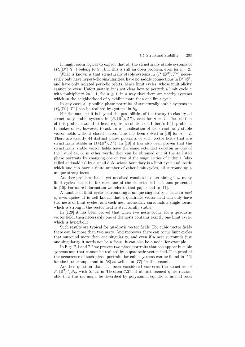
7.5 Structural Stability 203
It might seem logical to expect that all the structurally stable systems of(Pn(D2), T n) belong to Sn, but this is still an open problem, even for n = 2.
What is known is that structurally stable systems in (Pn(D2), T n) neces-sarily only have hyperbolic singularities, have no saddle connections in D
2 \S1,and have only isolated periodic orbits, hence limit cycles, whose multiplicitycannot be even. Unfortunately, it is not clear how to perturb a limit cycle γwith multiplicity 2n + 1, for n ≥ 1, in a way that there are nearby systemswhich in the neighborhood of γ exhibit more than one limit cycle.
In any case, all possible phase portraits of structurally stable systems in(Pn(D2), T n) can be realized by systems in Sn.
For the moment it is beyond the possibilities of the theory to classify allstructurally stable systems in (Pn(D2), T n), even for n = 2. The solutionof this problem would at least require a solution of Hilbert’s 16th problem.It makes sense, however, to ask for a classification of the structurally stablevector fields without closed curves. This has been solved in [10] for n = 2.There are exactly 44 distinct phase portraits of such vector fields that arestructurally stable in (P2(D
2), T 2). In [10] it has also been proven that thestructurally stable vector fields have the same extended skeleton as one ofthe list of 44, or in other words, they can be obtained out of the 44 listedphase portraits by changing one or two of the singularities of index 1 (alsocalled antisaddles) by a small disk, whose boundary is a limit cycle and insidewhich one can have a finite number of other limit cycles, all surrounding aunique strong focus.
Another problem that is yet unsolved consists in determining how manylimit cycles can exist for each one of the 44 extended skeletons presentedin [10]. For more information we refer to that paper and to [11].
A number of limit cycles surrounding a unique singularity is called a nestof limit cycles. It is well known that a quadratic vector field can only havetwo nests of limit cycles, and each nest necessarily surrounds a single focus,which is strong if the vector field is structurally stable.
In [129] it has been proved that when two nests occur, for a quadraticvector field, then necessarily one of the nests contains exactly one limit cycle,which is hyperbolic.
Such results are typical for quadratic vector fields. For cubic vector fieldsthere can be more than two nests. And moreover there can occur limit cyclesthat surround more than one singularity, and even if a nest surrounds justone singularity it needs not be a focus; it can also be a node, for example.
In Figs. 7.1 and 7.2 we present two phase portraits that can appear in cubicsystems and that cannot be realized by a quadratic vector field. The proof ofthe occurrence of such phase portraits for cubic systems can be found in [56]for the first example and in [58] as well as in [77] for the second.
Another question that has been considered concerns the structure ofPn(D2) \ Sn, with Sn as in Theorem 7.27. It at first seemed quite reason-able that this set might be described by polynomial equations, as had been
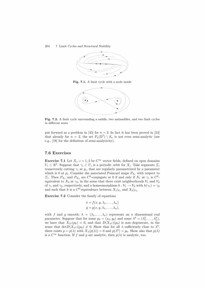
204 7 Limit Cycles and Structural Stability
Fig. 7.1. A limit cycle with a node inside
Fig. 7.2. A limit cycle surrounding a saddle, two antisaddles, and two limit cyclesin different nests
put forward as a problem in [45] for n = 2. In fact it has been proved in [54]that already for n = 2, the set Pn(D2) \ Sn is not even semi-analytic (seee.g., [18] for the definition of semi-analyticity).
7.6 Exercises
Exercise 7.1 Let Xi, i = 1, 2 be C∞ vector fields, defined on open domainsUi ⊂ R2. Suppose that γi ⊂ Ui is a periodic orbit for Xi. Take segments Σi
transversely cutting γi at pi, that are regularly parametrized by a parameterwhich is 0 at pi. Consider the associated Poincare maps PXi
with respect toΣi. Then PX1
and PX2are C0-conjugate at 0 if and only if X1 at γ1 is C0-
equivalent to X2 at γ2, in the sense that there exist neighborhoods V1 and V2
of γ1 and γ2, respectively, and a homeomorphism h : V1 → V2 with h(γ1) = γ2
and such that h is a C0-equivalence between X1|V1and X2|V2
.
Exercise 7.2 Consider the family of equations
x = f(x, y, λ1, . . . , λn)
y = g(x, y, λ1, . . . , λn),
with f and g smooth; λ = (λ1, . . . , λn) represents an n dimensional realparameter. Suppose that for some p0 = (x0, y0) and some λ0 = (λ0
1, . . . , λ0n),
we have that Xλ0(p0) = 0, and that D(Xλ0)(p0) is non–degenerate, in thesense that detD(Xλ0)(p0) �= 0. Show that for all λ sufficiently close to λ0,there exists p = p(λ) with Xλ(p(λ)) = 0 and p(λ0) = p0. Show also that p(λ)is a C∞ function. If f and g are analytic, then p(λ) is analytic, too.
7.6 Exercises 205
Exercise 7.3 Consider the same system as in the previous exercise, but sup-pose that D(Xλ0)(p0) is hyperbolic. Show that for λ ≈ λ0:
(i) D(Xλ)(pλ) is hyperbolic, too.(ii)Xλ at p(λ) is C0-conjugate to Xλ0 at p0. (We say that Xλ0 at p0 is locally
structurally stable).
Exercise 7.4 Let f : U ⊂ Rm → Rn be a C∞ function with U open. Sard’sTheorem states that almost all b ∈ Rn (with respect to Lebesgue measure)are regular values of f , meaning that either b /∈ f(U) or at all x ∈ f−1(b) wehave that Dfx : Rm → Rn is surjective.
(i) Let b ∈ f(U) be a regular value of f ; show that f−1(b) ⊂ U is a (m − n)dimensional submanifold of U .
(ii)Use Sard’s Theorem and point (i) to show that for any C∞ vector field Xon U ⊂ R2 with U open, and X(0) = 0, there exists a vector field havingan expression X + ε with ε ∈ R2, and ε arbitrarily close to 0, such that allsingularities of X + ε in U are non–degenerate.
Exercise 7.5 Let X : U ⊂ R2 → R2 be a C∞ vector field X = X1∂∂x +X2
∂∂y
having at 0 a non–degenerate singularity. Consider the following family ofvector fields X(a, b, c, d) depending on the four parameters (a, b, c, d):
x = ax + by + X1(x, y)
y = cx + dy + X2(x, y).
Show that there exist (a, b, c, d) arbitrarily close to (0, 0, 0, 0) such that Xa,b,c,d
has a hyperbolic singularity at (x, y) = (0, 0).
Exercise 7.6 Let X be a C∞ vector field on some open domain U ⊂ R2 andsuppose that at p ∈ U , X has a semi-hyperbolic singularity which is a genericsaddle-node, i.e., the restriction of X to any center manifold W c starts withquadratic terms with respect to a regular parametrization of W c. Show theexistence of a 1-parameter family Xε, a neighborhood V ⊂ U of p and anε0 > 0 such that for all ε ∈ (0, ε0), Xε has no singularities in V , while for allε ∈ (−ε0, 0), Xε has two singularities in V .
Hint: Use a normal form.
Exercise 7.7 Consider the previous exercise again, replacing the genericsaddle-node singularity by a generic nilpotent cusp point.
Exercise 7.8 Let Xλ = Xλ1,...,λnbe a smooth n-parameter family of vector
fields on some open subset U ⊂ R2 with λ ∈ B(λ0, ε). Suppose that Xλ0
has a hyperbolic limit cycle γ0. Show that there exists a 0 < δ < ε and aneighborhood V of γ0 in U such that for all λ ∈ B(λ0, δ), Xλ has a uniqueperiodic orbit in V . Moreover the periodic orbit is hyperbolic and Xλ|V isC0-equivalent to Xλ0 |V . Extra question: Can we be sure that Xλ|V is C0-conjugate to Xλ0 |V ? If so, give a proof, if not, give a counterexample.
Hint: Use a Poincare map.
206 7 Limit Cycles and Structural Stability
Exercise 7.9 Let X be a smooth vector field defined on some open subset ofR2 and let Xa, for a ∈ R and a ≈ 0 be a smooth rotated family of vector fields.Suppose that X has γ as a limit cycle of even multiplicity (γ is semistable).Show that for a �= 0 and a ≈ 0, Xa has either no closed curves, or at leasttwo.
Hint: Use the Poincare–Bendixson Theorem.
Exercise 7.10 Consider the ε-family of smooth Lienard system Xε
x = y,
y = g(x) + yf(x) + εy,
such that for ε = 0 the system X0 has a hyperbolic saddle at both p1 = (x1, 0)and p2 = (x2, 0) together with a heteroclinic connection between them. Showthat for ε �= 0, ε ≈ 0, system Xε has no heteroclinic connection between p1
and p2.Hint: Use the property of rotated vector fields.
Exercise 7.11 Let f1, f2 be C2 functions on R2. Given a > 0 prove that anecessary condition for the system
x = y + μf1(x, y),
y = − x + μf2(x, y),(7.22)
to have a periodic solution ϕ(t, a, μ) of period τ(μ) for every μ sufficientlysmall is that ϕa = ϕ(t, q, 0) = a(cos t,− sin t) and τ(μ) is differentiable withτ(0) = 2π, and that
β(a) =
∫
ϕa
f1dy + f2dx = 0.
Prove that if β(a) = 0 and β′(a) �= 0, then (7.22) in fact has the propertiesdescribed above.
Hint: Use polar coordinates x = r cos θ, y = r sin θ transforming (7.22)into
r = μR1(r, θ, μ),
θ = 1 + R2(r, θ, μ),
which is equivalent to an equation of the type
dr
dθ= μR(r, θ, μ). (7.23)
Prove that a solution of (7.23) is of the form ρ(r, θ, μ) = r+μβ(r)+ε(r, t)μ.
Exercise 7.12 Use the previous exercise to prove that the equation of vander Pol
x′′ = −x + εx′(1 − x2)

7.6 Exercises 207
has, for every ε > 0 sufficiently small, a unique limit cycle stable in a neigh-borhood of the circle x2 + (x′)2 = 4. Prove also that as ε → 0, this limit cycletends to the given circle.
Exercise 7.13 Let X = (X1, X2) be a vector field on R2, where
X1 = y + x(1 − x2 − y2)
X2 = − x + y(1 − x2 − y2).
Prove that this vector field has a unique periodic orbit γ. Find a Poincaremap π associated to γ and prove that π′ �= 1 at γ.
Hint: In polar coordinates the system above becomes
r = r(1 − r2),
θ = − 1.
Show that ∫dr
r(1 − r2)=
1
2log
(r2
1 − r2
),
and then show that π : R+ → R+ (where R+ denotes the positive x–axis) isgiven by
π(r) =reπ
√1 − r2 + r2e2π
.
Exercise 7.14 Let γ be a stable periodic orbit of X = (X1, X2). Let
Xθ =
(cos θ sin θ− sin θ cos θ
)(X1
X2
).
This is the vector field obtained from X after doing a rotation of angle θ.
(i) Prove that there exists ε > 0 such that Xθ with |θ| < ε has a periodicorbit γθ such that γθ → γ when θ → 0.
(ii) Prove that the γθ are all disjoint, that is
γθ1∩ γθ2
= ∅ if θ1 �= θ2,
and prove that⋃
|θ|≤ε γθ is an annular region of the plane.
(iii) If γ is an unstable periodic orbit prove an analogous version of (i) and (ii).(iv) If γ is semistable prove that for θ with appropriate sign (positive or
negative depending on the case), there exist two periodic orbits γθ1and
γθ2with γθi
→ γ when θ → 0, for i = 1, 2.
Exercise 7.15 Show that the systems
x′′ + (5x4 − 9x2)x′ + x5 = 0,
x′′ + (x6 − x2)x′ + x = 0,
have a periodic orbit.

208 7 Limit Cycles and Structural Stability
Exercise 7.16 Prove Poincare’s Theorem: A planar analytic system x =f(x), cannot have an infinite number of limit cycles which accumulate ona limit cycle of the system.
Exercise 7.17 Show that γ(t) = (2 cos 2t, sin 2t) is a periodic solution of thesystem
x = − 4y + x
(1 − x2
4− y2
),
y =x + y
(1 − x2
4− y2
),
that lies in the ellipse (x/2)2 + y2 = 1; i.e., γ(t) represents a cycle Γ of thissystem. Then show that Γ is a stable limit cycle.
Exercise 7.18 Show that the system
x = − y + x(1 − x2 − y2)2,
y =x + y(1 − x2 − y2)2,
has a limit cycle Γ represented by γ(t) = (cos t, sin t). Show that Γ is amultiple limit cycle. Since Γ is a semistable limit cycle, we know that themultiplicity k of Γ is even. Can you show that k = 2?
Exercise 7.19 Use the Poincare–Bendixson Theorem and the fact that theplanar system
x =x − y − x3,
y =x + y − y3,
has only a single singular point at the origin to show that this system has aperiodic orbit in the annular region A = {x ∈ R2 : 1 ≤ |x| ≤
√2}.
Hint: Convert to polar coordinates and show that for all ε > 0, r < 0 onthe circle r =
√2 + ε and r > 0 on r = 1 − ε.
Exercise 7.20 Following exercise 7.20 show that there is at least one stablelimit cycle in A (In fact this system has exactly one limit cycle in A and it isstable.)
Exercise 7.21 Show that
x = y,
y = − x + (1 − x2 − y2)y,
has a unique stable limit cycle which is the ω-limit set of every trajectoryexcept the singular point at the origin.
Hint: Compute r.
7.6 Exercises 209
Exercise 7.22 Use the Dulac function B(x, y) = be−2βx to show that thesystem
x = y,
y = − ax − by + αx2 + βy2,
has no limit cycle in R2.
Exercise 7.23 Show that the system
x =y
1 + x2,
y =−x + y(1 + x2 + x4)
1 + x2,
has no limit cycle in R2.
Exercise 7.24 Prove that the system
x = δx − y + x2 + mxy + ny2,
y =x + bxy,
with b = [(1 + n)2 + δ(m + mn + δn)]/(δ2n), δn(1 + n) �= 0 and n > 0, has noperiodic orbits.
Hint: Use the fact that this system has an inverse polynomial integratingfactor of degree 2.
Exercise 7.25 Let x = P (x, y) and y = Q(x, y) be a quadratic polynomialdifferential equation. Prove that if the pencil of conics P + λQ contains animaginary conic, a real conic reduced to a single point, or a double straightline, then the system has no periodic orbits.
Hint: Use Theorem 7.15 with V = ex+λ0y, where P + λ0Q is one of theconics mentioned.
Exercise 7.26 Consider the system
x = − y + ax(x2 + y2 − 1),
y =x + by(x2 + y2 − 1).
Let γ = {(x, y) ∈ R2 : x2 + y2 = 1}. Prove:
(i) if a + b = 0 and ab �= 0, then γ is the unique limit cycle of the system.Hint: Use Theorem 7.16.
(ii)if a + b �= 0, then γ is a hyperbolic limit cycle, stable if a + b < 0 andunstable if a + b > 0.
Exercise 7.27 Consider the system
x = y − (a1x + a2x2 + a3x
3 + x4),
y = − x.

210 7 Limit Cycles and Structural Stability
For fixed a2, a3 ∈ R, show that this system defines a family of generalizedrotated vector fields with respect to the parameter a1.
Exercise 7.28 Consider the system
x = − x + y2,
y = − μx + y + μy2 − xy.
Using the fact that μ is a generalized rotation parameter for this system,describe the phase portrait of the system in the Poincare disk as μ varies inR. Note that as μ is changed this system has a simultaneous Hopf bifurcationof limit cycles at the foci (1, 1) after μ = 1/2 and that both limit cyclesend simultaneously in two homoclinic loops of the saddle (0, 0) at μ ≈ 0.52.Note also that this system is invariant under the transformation (x, y, μ) →(x,−y,−μ).
7.7 Bibliographical Comments
This chapter follows partly the book of Ye Yan Qian et al. (see [135]). Sect. 7.2follows the paper [102]. In 1900 Hilbert [82], in the second part of his 16thproblem, proposed finding an uniform upper bound on the number of limitcycles of all polynomial vector fields of a given degree, and also studying theirdistribution or configuration in the plane. This has been one of the mainproblems in the qualitative theory of planar differential equations in the 20thcentury. The contributions of Bamon [13], Golitsina [73] and Kotova [97] forthe particular case of quadratic vector fields, and mainly of Ecalle [59] andIl’yashenko [88] in proving that any polynomial vector field has but finitelymany limit cycles have been the best results in this area. But until now it hasnot been proved that there exists an uniform upper bound depending only onthe degree. This problem remains open even for quadratic polynomial vectorfields.
People interested in 16th Hilbert’s problem, concerning the maximumnumber of limit cycles which polynomial vector fields of a given degree canhave, can also have a look at [89].
The problem of the realization of a given configuration of closed curvesby a polynomial differential system has been studied by several authors. ForCr vector fields the problem was solved by Al’mukhamedov [1], Balibrea andJimenez [12] and Valeeva [158]. Statement (i) of Theorem 7.18 was solvedby Schecter and Singer [140] and Sverdlove [155], but they did not providean explicit polynomial vector field satisfying the given configuration of limitcycles. The result presented in statement (ii) of Theorem 7.18 appears in[102], and its proof provides simultaneously the shortest and easiest proof ofstatement (i) of Theorem 7.18.
There are relatively complete results on the rotated vector field theory. Theearliest work can be found in the paper [50] of Duff in 1953. Later, Seifert [145],
7.7 Bibliographical Comments 211
Perko [127] and Chen Xiang-Yan [165–167], successively improved the work ofDuff. We should especially note that Chen Xiang-Yan introduced the conceptof generalized rotated vector fields, which greatly weakens the conditions ofDuff, and leads to important applications of rotated vector fields.
For additional information about general results on limit cycles in planarpolynomial differential systems see [169].

8
Integrability and Algebraic Solutionsin Polynomial Vector Fields
In contrast to earlier chapters, throughout this chapter we will work withcomplex two-dimensional differential systems, although our main aim stillremains in the study of real planar differential equations.
For a two-dimensional vector field the existence of a first integral com-pletely determines its phase portrait. The simplest planar vector fields havinga first integral are the Hamiltonian ones. The integrable planar vector fieldswhich are not Hamiltonian are, in general, very difficult to detect. In thischapter we study the existence of first integrals for planar polynomial vectorfields through the Darbouxian theory of integrability. This kind of integrabi-lity provides a link between the integrability of polynomial vector fields andthe number of invariant algebraic curves that they have.
8.1 Introduction
By definition a two-dimensional complex planar polynomial differential systemor simply a polynomial system will be a differential system of the form
dx
dt= x = P (x, y),
dy
dt= y = Q(x, y), (8.1)
where the dependent variables x and y, and the independent one (the time)t are complex, and P and Q are polynomials in the variables x and y withcomplex coefficients. Throughout this chapter m = max{deg P,deg Q} de-notes the degree of the polynomial system, and we always assume that thepolynomials P and Q are relatively prime in the ring of complex polynomialsin the variables x and y.
We want to show the fascinating relationships between integrability (atopological phenomenon) and the existence of exact algebraic solutions for apolynomial system.

214 8 Integrability and Algebraic Solutions in Polynomial Vector Fields
8.2 First Integrals and Invariants
We denote by F either the real field R or the complex field C; and by anF-polynomial system the polynomial system (8.1) with the variables x, y andthe coefficients of the polynomials P and Q in F. We also denote by F[x, y]the ring of polynomials in the variables x and y and coefficients in F.
The vector field X associated to system (8.1) is defined by
X = P∂
∂x+ Q
∂
∂y.
The F-polynomial system (8.1) is integrable on an open subset U of F2 ifthere exists a nonconstant analytic function H : U → F, called a first integralof the system on U , which is constant on all solution curves (x(t), y(t)) ofsystem (8.1) contained in U ; i.e., H(x(t), y(t)) = constant for all values of tfor which the solution (x(t), y(t)) is defined and contained in U . Clearly H isa first integral of system (8.1) on U if and only if XH = PHx + QHy ≡ 0on U .
Let U ⊂ F2 be an open set. We say that an analytic function H(x, y, t) :U×F → F is an invariant of the polynomial vector field X on U if H(x, y, t) =constant for all values of t for which the solution (x(t), y(t)) is defined andcontained in U . If an invariant H is independent of t then of course it is afirst integral.
The knowledge provided by an invariant is weaker than the one providedby a first integral. The invariant, in general, gives information only abouteither the α- or the ω-limit set of the orbits of the system.
8.3 Integrating Factors
Let U be an open subset of F2 and let R : U → F be an analytic functionwhich is not identically zero on U . The function R is an integrating factor ofthe F-polynomial system (8.1) on U if one of the following three equivalentconditions holds on U :
∂(RP )
∂x= −∂(RQ)
∂y, div(RP,RQ) = 0, XR = −R div(P,Q).
As usual the divergence of the vector field X is defined by
div(X) = div(P,Q) =∂P
∂x+
∂Q
∂y.
The first integral H associated to the integrating factor R is given by
H(x, y) =
∫R(x, y)P (x, y) dy + h(x), (8.2)
8.4 Invariant Algebraic Curves 215
where h is chosen such that ∂H∂x
= −RQ. Then
x = RP =∂H
∂y, y = RQ = −∂H
∂x. (8.3)
In (8.2) we suppose that the domain of integration U is well adapted tothe specific expression.
Conversely, given a first integral H of system (8.1) we always can find anintegrating factor R for which (8.3) holds.
Proposition 8.1 If the F-polynomial system (8.1) has two integrating factorsR1 and R2 on the open subset U of F2, then in the open set U \ {R2 = 0} thefunction R1/R2 is a first integral, provided R1/R2 is non-constant.
Proof. Since Ri is an integrating factor, it satisfies XRi = −Ridiv(P,Q) fori = 1, 2. Therefore the proposition follows immediately from the computation
X
(R1
R2
)=
(XR1)R2 − R1(XR2)
R22
= 0. �
8.4 Invariant Algebraic Curves
Let f ∈ C[x, y], f not identically zero. The algebraic curve f(x, y) = 0 isan invariant algebraic curve of the F-polynomial system (8.1) if for somepolynomial K ∈ C[x, y] we have
Xf = P∂f
∂x+ Q
∂f
∂y= Kf. (8.4)
The polynomial K is called the cofactor of the invariant algebraic curve f = 0.We note that, since the polynomial system has degree m, any cofactor hasdegree at most m − 1.
On the points of the algebraic curve f = 0 the gradient (∂f/∂x, ∂f/∂y)of f is orthogonal to the vector field X = (P,Q) (see (8.4)). Hence at everypoint of f = 0 the vector field X is tangent to the curve f = 0, so the curvef = 0 is formed by trajectories of the vector field X. This justifies the name“invariant algebraic curve” since it is invariant under the flow defined by X.
We remark that in the definition of invariant algebraic curve f = 0 wealways allow this curve to be complex; that is f ∈ C[x, y] even in the case of areal polynomial system. As we will see this is due to the fact that sometimesfor real polynomial systems the existence of a real first integral can be forcedby the existence of complex invariant algebraic curves. Of course when welook for a complex invariant algebraic curve of a real polynomial system weare thinking of the real polynomial system as a complex one.
In the next proposition and throughout the whole chapter (complex) con-jugation stands for conjugation of the coefficients of the polynomials only.This amounts of course to generic conjugation if we restrict the variables to(x, y) ∈ R2

216 8 Integrability and Algebraic Solutions in Polynomial Vector Fields
Proposition 8.2 For a real polynomial system (8.1), f = 0 is an invariantalgebraic curve with cofactor K if and only if f = 0 is an invariant algebraiccurve with cofactor K.
Proof. We assume that f = 0 is an invariant algebraic curve with cofactor Kof the real polynomial system (8.1). Then equality (8.4) holds. Since P andQ are real polynomials conjugating equality (8.4) we obtain
P∂f
∂x+ Q
∂f
∂y= Kf .
Consequently, f = 0 is an invariant algebraic curve with cofactor K of system(8.1). The proof in the converse is similar. �
Lemma 8.3 Let f, g ∈ C[x, y]. We assume that f and g are relatively primein the ring C[x, y]. Then for a polynomial system (8.1), fg = 0 is an invariantalgebraic curve with cofactor Kfg if and only if f = 0 and g = 0 are invariantalgebraic curves with cofactors Kf and Kg, respectively. Moreover, Kfg =Kf + Kg.
Proof. It is clear that
X(fg) = (Xf)g + f(Xg). (8.5)
We assume that fg = 0 is an invariant algebraic curve of system (8.1) withcofactor Kfg. Then X(fg) = Kfgfg and from equality (8.5) we get Kfgfg =(Xf)g + fXg. Therefore, since f and g are relatively prime, we obtain that fdivides Xf , and g divides Xg. If we denote by Kf the quotient Xf/f and byKg the quotient Xg/g, then f = 0 and g = 0 are invariant algebraic curves ofsystem (8.1) with cofactors Kf and Kg, respectively, and Kfg = Kf + Kg.
The proof of the converse follows in a similar way, again using equality(8.5). ⊓⊔
Proposition 8.4 Suppose f ∈ C[x, y] and let f = fn1
1 . . . fnrr be its factoriza-
tion into irreducible factors over C[x, y]. Then for a polynomial system (8.1),f = 0 is an invariant algebraic curve with cofactor Kf if and only if fi = 0 isan invariant algebraic curve for each i = 1, . . . , r with cofactor Kfi
. MoreoverKf = n1Kf1
+ . . . + nrKfr.
Proof. From Lemma 8.3, we know that f = 0 is an invariant algebraic curvewith cofactor Kf if and only if fni
i = 0 is an invariant algebraic curve for eachi = 1, . . . , r with cofactor Kf
nii
; furthermore Kf = Kfn11
+ . . . + Kfnrr
.
Now to prove the proposition it is sufficient to show, for each i = 1, . . . , r,that fni
i = 0 is an invariant algebraic curve with cofactor Kfnii
if and only
if fi = 0 is an invariant algebraic curve with cofactor Kfi, and that Kf
nii
=
niKfi. We assume that fni
i = 0 is an invariant algebraic curve with cofactorKf
nii
. Then
8.5 Exponential Factors 217
Kfnii
fni
i = X (fni
i ) = nifni−1i X(fi),
or equivalently
X(fi) =1
niKf
nii
fi.
So defining Kfi= Kf
nii
/ni we obtain that fi = 0 is an invariant algebraic
curve with cofactor Kfisuch that Kf
nii
= niKfi. The proof of the converse
follows in a similar way. �
An irreducible invariant algebraic curve f = 0 will be an invariant algebraiccurve such that f is an irreducible polynomial in the ring C[x, y].
8.5 Exponential Factors
There is another object, the so-called exponential factor, that plays thesame role as the invariant algebraic curves in obtaining a first integral ofthe polynomial system (8.1). Before defining it formally, we explain howthe notation arises naturally. Suppose we have invariant algebraic curveshε = h + εg + O(ε2) = 0 with cofactors Khε
for ε ∈ [0, ε0] with ε0 suffi-ciently small. Using the fact that X(hε) = Khε
hε, if we expand the cofactorKhε
as a power series in ε we obtain that Khε= Kh + εK + O(ε2), where K
is some polynomial of degree at most m − 1. We can now make a local studynear a point where h is not zero.
Since
X
(hε
h
)=
X(hε)h − (hε)Xh
h2
=Khε
(hε)h − (hε)Khh
h2
=(Kh + εK + O(ε2))(h + εg + O(ε2))h − (h + εg + O(ε2))Khh
h2
= εK + O(ε2),
we have
X
((hε
h
) 1ε
)=
1
ε
(hε
h
) 1ε(
hε
h
)−1
X
(hε
h
)
=1
ε
(hε
h
) 1ε
(1 + O(ε))(εK + O(ε2)
)(8.6)
= (K + O(ε))
(hε
h
) 1ε
.
Therefore the function (h + εg + O(ε2)
h
) 1ε
218 8 Integrability and Algebraic Solutions in Polynomial Vector Fields
has cofactor K + O(ε). As ε tends to zero, the expression above tends to
exp( g
h
), (8.7)
and from (8.6) we obtain that
X(exp
( g
h
))= K exp
( g
h
). (8.8)
Therefore, function (8.7) satisfies the same equation (8.4) as do the invariantalgebraic curves, with a cofactor of degree at most m − 1.
Let h, g ∈ C[x, y] and assume that h and g are relatively prime in the ringC[x, y] or that h ≡ 1. Then the function exp(g/h) is called an exponentialfactor of the F-polynomial system (8.1) if for some polynomial K ∈ C[x, y] ofdegree at most m − 1 it satisfies equation (8.8). As before we say that K isthe cofactor of the exponential factor exp(g/h).
As we will see, from the point of view of the integrability of polynomialsystems (8.1) the importance of the exponential factors is twofold. On theone hand, they satisfy equation (8.8), and on the other hand, their cofactorsare polynomials of degree at most m − 1. These two facts mean that theyplay the same role as the invariant algebraic curves in the integrability of apolynomial system (8.1). We note that the exponential factors do not defineinvariant curves for the flow of system (8.1), because they are never zero.
We remark that in the definition of exponential factor exp(g/h) we alwaysallow that this function be complex; that is h, g ∈ C[x, y] even in the case ofa real polynomial system. The reason is the same as in the case of invariantalgebraic curves. That is, sometimes for real polynomial systems the existenceof a real first integral can be forced by the existence of complex exponentialfactors. Again, in looking for a complex exponential factor of a real polynomialsystem, we consider the real polynomial system as being on C2.
Proposition 8.5 For a real polynomial system (8.1) the function exp(g/h)is an exponential factor with cofactor K if and only if the function exp(g/h)is an exponential factor with cofactor K.
Proof. We assume that exp(g/h) is an exponential factor of the real polyno-mial system (8.1) with cofactor K. Then equality (8.8) holds. Since P and Qare real polynomials, conjugating equality (8.8) we obtain that
P∂ exp(g/h)
∂x+ Q
∂ exp(g/h)
∂y= K exp(g/h).
Consequently, exp(g/h) is an exponential factor of system (8.1) with cofactorK. The proof of the converse is similar. �
Proposition 8.6 If F = exp(g/h) is an exponential factor for the polynomialsystem (8.1), then h = 0 is an invariant algebraic curve, and g satisfies theequation
Xg = gKh + hKF ,
where Kh and KF are the cofactors of h and F , respectively.
8.6 The Method of Darboux 219
Proof. Since F = exp(g/h) is an exponential factor with cofactor KF , we have
KF exp( g
h
)= X
(exp
( g
h
))
= exp( g
h
)X( g
h
)= exp
( g
h
) (Xg)h − g(Xh)
h2,
or equivalently(Xg)h − g(Xh) = h2KF .
Hence since h and g are relatively prime, we obtain that h divides Xh. Soh = 0 is an invariant algebraic curve with cofactor Kh = Xh/h. Now replacingXh by Khh in the last equality, we have that Xg = gKh + hKF . �
In fact, the way that the exponential factor exp(g/h) has been introducedat the beginning of this section implies that it appears when the invariantalgebraic curve h = 0 has geometric multiplicity higher than 1.
8.6 The Method of Darboux
Before stating the main results of the Darboux theory we need some defini-tions. If S(x, y) =
∑m−1i+j=0 aijx
iyj is a polynomial of degree at most m − 1with m(m + 1)/2 coefficients in F, then we write S ∈ Fm−1[x, y]. We identifythe linear vector space Fm−1[x, y] with Fm(m+1)/2 through the isomorphism
S → (a00, a10, a01, . . . , am−1,0, am−2,1, . . . , a0,m−1).
We say that r points (xk, yk) ∈ F2, k = 1, . . . , r, are independent withrespect to Fm−1[x, y] if the intersection of the r hyperplanes
m−1∑
i+j=0
xikyj
kaij = 0, k = 1, . . . , r,
in Fm(m+1)/2 is a linear subspace of dimension [m(m + 1)/2] − r.We remark that the maximum number of isolated singular points of the
polynomial system (8.1) is m2 (by Bezout’s Theorem), that the maximumnumber of independent isolated singular points of the system is m(m + 1)/2,and that m(m + 1)/2 < m2 for m ≥ 2.
A singular point (x0, y0) of system (8.1) is called weak if the divergence,div(P,Q), of system (8.1) at (x0, y0) is zero.
Theorem 8.7 [Darboux Theory of integrability for complex polynomial sys-tems] Suppose that a C-polynomial system (8.1) of degree m admits p irre-ducible invariant algebraic curves fi = 0 with cofactors Ki for i = 1, . . . , p, qexponential factors exp(gj/hj) with cofactors Lj for j = 1, . . . , q, and r inde-pendent singular points (xk, yk) ∈ C2 such that fi(xk, yk) �= 0 for i = 1, . . . , pand for k = 1, . . . , r.

220 8 Integrability and Algebraic Solutions in Polynomial Vector Fields
(i) There exist λi, μj ∈ C not all zero such that∑p
i=1 λiKi +∑q
j=1 μjLj = 0,if and only if the (multivalued) function
fλ1
1 . . . fλpp
(exp
(g1
h1
))µ1
. . .
(exp
(gq
hq
))µq
(8.9)
is a first integral of system (8.1).(ii) If p + q + r ≥ [m(m + 1)/2] + 1, then there exist λi, μj ∈ C not all zero
such that∑p
i=1 λiKi +∑q
j=1 μjLj = 0.(iii) If p + q + r ≥ [m(m + 1)/2] + 2, then system (8.1) has a rational first
integral, and consequently all trajectories of the system are contained ininvariant algebraic curves.
(iv) There exist λi, μj ∈ C not all zero such that∑p
i=1 λiKi +∑q
j=1 μjLj =−div(P,Q), if and only if function (8.9) is an integrating factor of system(8.1).
(v) If p+q+r = m(m+1)/2 and the r independent singular points are weak,then function (8.9) is a first integral if
∑pi=1 λiKi +
∑qj=1 μjLj = 0, or
an integrating factor if∑p
i=1 λiKi +∑q
j=1 μjLj = −div (P,Q), under thecondition that not all λi, μj ∈ C are zero.
(vi) If there exist λi, μj ∈ C not all zero such that∑p
i=1 λiKi +∑q
j=1 μjLj =−s for some s ∈ C \ {0}, then the (multivalued) function
fλ1
1 . . . fλpp
(exp
(g1
h1
))µ1
. . .
(exp
(gq
hq
))µq
exp(st)
is an invariant of system (8.1).
Of course, each irreducible factors of each hj is one of the fi’s.
Proof of Theorem 8.7: We write Fj = exp(gj/hj). By hypothesis we have pinvariant algebraic curves fi = 0 with cofactors Ki, and q exponential factorsFj with cofactors Lj . That is, the fis satisfy Xfi = Kifi, and the Fjs satisfyXFj = LjFj .(i) Clearly statement (i) follows from the fact that
X(fλ1
1 . . . fλpp Fµ1
1 . . . Fµqq
)=
(fλ1
1 . . . fλpp Fµ1
1 . . . Fµqq
)⎛⎝
p∑
i=1
λiXfi
fi+
q∑
j=1
μjXFj
Fj
⎞⎠ =
(fλ1
1 . . . fλpp Fµ1
1 . . . Fµqq
),
⎛⎝
p∑
i=1
λiKi +
q∑
j=1
μjLj
⎞⎠ = 0.
(ii) Since the cofactors Ki and Lj are polynomials of degree m − 1, we havethat Ki, Lj ∈ Cm−1[x, y]. We note that the dimension of Cm−1[x, y] as avector space over C is m(m + 1)/2.
8.6 The Method of Darboux 221
Since (xk, yk) is a singular point of system (8.1), P (xk, yk) = Q(xk, yk) =0. Then from Dfi = P (∂fi/∂x) + Q(∂fi/∂y) = Kifi, it follows thatKi(xk, yk)fi(xk, yk) = 0. As we have assumed that fi(xk, yk) �= 0, thereforeKi(xk, yk) = 0 for i = 1, . . . , p. Again, from DFj = P (∂Fj/∂x)+Q(∂Fj/∂y) =LjFj , it follows that Lj(xk, yk)Fj(xk, yk) = 0. Since Fj = exp(gj/hj) doesnot vanish, Lj(xk, yk) = 0 for j = 1, . . . , q. Consequently, since the r singu-lar points are independent, all the polynomials Ki and Lj belong to a linearsubspace S of Cm−1[x, y] of dimension [m(m+1)/2]−r. We have p+q polyno-mials Ki and Lj and since from the assumptions p+ q > [m(m+1)/2]− r, weobtain that the p + q polynomials must be linearly dependent in S. So thereare λi, μj ∈ C not all zero such that
∑pi=1 λiKi +
∑qj=1 μjLj = 0. Hence
statement (ii) is proved.(iii) Since the number of independent singular points r ≤ m(m + 1)/2, itfollows that p + q ≥ 2. Under the assumptions of statement (iii) we applystatement (ii) to two subsets of p + q − 1 > 0 functions defining invariantalgebraic curves or exponential factors. Thus we get two linear dependenciesbetween the corresponding cofactors, which after some linear algebra andrelabeling, we can write in the following form
M1+α3M3+ . . .+αp+q−1Mp+q−1 = 0, M2+β3M3+ . . .+βp+q−1Mp+q−1 = 0,
where Ml are the cofactors Ki and Lj , and the αl and βl are complex numbers.Then by statement (i), it follows that the two functions
G1Gα3
3 . . . Gαp+q−1
p+q−1 , G2Gβ3
3 . . . Gβp+q−1
p+q−1 ,
are first integrals of system (8.1), where Gl is the polynomial defining aninvariant algebraic curve or the exponential factor having cofactor Ml forl = 1, . . . , p + q − 1. Then taking logarithms of the two first integrals above,we obtain that
H1 = log(G1) + α3 log(G3) + . . . + αp+q−1 log(Gp+q−1),
H2 = log(G2) + β3 log(G3) + . . . + βp+q−1 log(Gp+q−1),
are first integrals of system (8.1) on their domain of definition. Each providesan integrating factor Ri such that
P = Ri∂Hi
∂y, Q = −Ri
∂Hi
∂x.
Therefore, we obtain that
R1
R2=
∂H2
∂x/∂H1
∂x.
Since the functions Gl are polynomials or exponentials of a quotient ofpolynomials, it follows that the functions ∂Hi/∂x are rational for i = 1, 2. So
222 8 Integrability and Algebraic Solutions in Polynomial Vector Fields
from the last equality, we get that the quotient of the two integrating factorsR1/R2 is a rational function. Proposition 8.1 implies statement (iii).(iv) Since the equality
∑pi=1 λiKi +
∑qj=1 μjLj = −div(P,Q) is equivalent to
the equality
X(fλ1
1 . . . fλpp Fµ1
1 . . . Fµqq
)=
(fλ1
1 . . . fλpp Fµ1
1 . . . Fµqq
)⎛⎝
p∑
i=1
λiKi +
q∑
j=1
μjLj
⎞⎠ =
−(fλ1
1 . . . fλpp Fµ1
1 . . . Fµqq
)div(P,Q) ,
statement (iv) follows.(v) Let K = div(P,Q); clearly K ∈ Cm−1[x, y]. By assumption the r singularpoints (xk, yk) are weak, therefore K(xk, yk) = 0 for k = 1, . . . , r. So Kbelongs to the linear subspace S of the proof of statement (ii).
On the other hand, since dim S = p + q = [m(m + 1)/2] − r ≥ 0 andwe have p + q + 1 polynomials K1, . . . , Kp, L1, . . . , Lq, K in S (we are usingthe same arguments as in the proof of statement (ii)), it follows that thesepolynomials are linearly dependent in S. Therefore, we obtain λi, μj , α ∈ C
not all zero such that
(p∑
i=1
λiKi
)+
⎛⎝
q∑
j=1
μjLj
⎞⎠+ αK = 0. (8.10)
If α = 0 then as in the proof of statement (i), we obtain that function(8.9) is a first integral of system (8.1).
We assume now that α �= 0. Dividing the equality (8.10) by α (if nec-essary), we can assume without loss of generality that α = 1. So we havethat
K = −(
p∑
i=1
λiKi
)−
⎛⎝
q∑
j=1
μjLj
⎞⎠ .
Therefore, statement (v) follows from:
X(fλ1
1 . . . fλpp Fµ1
1 . . . Fµqq
)=
(fλ1
1 . . . fλpp Fµ1
1 . . . Fµqq
)⎛⎝
p∑
i=1
λiKi +
q∑
j=1
μjLj
⎞⎠ =
−(fλ1
1 . . . fλpp Fµ1
1 . . . Fµqq
)K =
−(fλ1
1 . . . fλpp Fµ1
1 . . . Fµqq
)div(P,Q) .
8.7 Some Applications of the Darboux Theory 223
(vi) We have λi, μj ∈ C not all zero such that∑p
i=1 λiKi +∑q
j=1 μjLj = −s.Then from
X(fλ1
1 . . . fλpp Fµ1
1 . . . Fµqq est
)=
(fλ1
1 . . . fλpp Fµ1
1 . . . Fµqq est
)⎛⎝
p∑
i=1
λiKi +
q∑
j=1
μjLj + s
⎞⎠ = 0 ,
statement (iv) follows.A (multivalued) function of the form (8.9) is called a Darbouxian function.Now we shall see that if the polynomial differential system is real, then
the first integral provided by the Darboux theory of integrability is also real.This follows from the following fact. Since the polynomial differential system(8.1) is real, it is well known that if a complex invariant algebraic curve orexponential factor appears, then its conjugate must appear simultaneously(see Propositions 8.2 and 8.5). If among the invariant algebraic curves of thereal system (8.1) a complex conjugate pair f = 0 and f = 0 occurs, thefunction (8.9) has a real factor of the form fλf λ, which is the multivaluedreal function
[(Re f)
2+ (Im f)
2]Reλ
exp (−2 Im λ arg (Re f + i Im f)) ,
if Imλ Im f �≡ 0. If among the exponential factors of the real system (8.1)a complex conjugate pair F = exp(h/g) and F = exp(h/g) occurs, the firstintegral (8.9) has a real factor of the form
(exp
(h
g
))µ(exp
(h
g
))µ
= exp
(2Re
(μ
h
g
)).
In short, the function (8.9) is real when the polynomial differential system(8.1) is real.
8.7 Some Applications of the Darboux Theory
In what follows we present applications of each statement of Darboux’s theo-rem to quadratic systems. For quadratic systems m(m + 1)/2 = 3
Example 8.8 If a �= 0 the quadratic system
x = −y(ay + b) − (x2 + y2 − 1), y = x(ay + b), (8.11)
has the algebraic solutions f1 = ay + b = 0 with cofactor K1 = ax, andf2 = x2 + y2 − 1 = 0 with cofactor K2 = −2x. Since 2K1 + aK2 = 0, byTheorem 8.7(i) we have that H = (ay + b)2(x2 + y2 − 1)a is a first integral ofsystem (8.11).

224 8 Integrability and Algebraic Solutions in Polynomial Vector Fields
Example 8.9 If abc �= 0 then the real quadratic system
x = x(ax + c), y = y(2ax + by + c), (8.12)
has exactly the following five invariant straight lines (i.e. algebraic solutionsof degree 1): f1 = x = 0, f2 = ax + c = 0, f3 = y = 0, f4 = ax + by = 0,f5 = ax + by + c = 0. Then by Theorem 8.7(ii) we know that system (8.5)must have a first integral of the form H = fλ1
1 fλ2
2 fλ3
3 fλ4
4 fλ5
5 with λi ∈ F
satisfying∑5
i=1 λiKi = 0, where Ki is the cofactor of fi. An easy computationshows that K1 = ax + c, K2 = ax, K3 = 2ax + by + c, K4 = ax + by + cand K5 = ax + by. Then a solution of
∑5i=1 λiKi = 0 is λ1 = λ5 = −1,
λ2 = λ4 = 1 and λ3 = 0. Therefore a first integral of system (8.12) is
H =(ax + c)(ax + by)
x(ax + by + c).
We note that since this system has 5 invariant algebraic curves, by Theorem8.7(iii) it must have a rational first integral, as we have found.
Example 8.10 The real quadratic system
x = −y − b(x2 + y2) = P, y = x = Q, (8.13)
has the invariant algebraic curve f1 = x2 +y2 with cofactor K1 = −2bx. SinceK1 = div(P,Q), from Theorem 8.7(iv), it follows that f−1
1 is an integratingfactor. Then an easy computation shows that H = exp(2by)(x2 + y2) is a firstintegral of system (8.13).
Example 8.11 If a02 �= 0 then the real quadratic system
x = x2 − 1 = P, y = a00 + a10x + a01y + a20x2 + a11xy + a02y
2 = Q,
with a00 = (2a11 + a201 − 1)/(4a02), a10 = a01a11/(2a02) and a20 = a11(a11 −
2)/(4a02), has the following three algebraic solutions: two straight lines f1 =x + 1, f2 = x − 1, and one hyperbola
f3 =a11(a11 − 2)
4a02x2+(a11−1)xy+a02y
2+a01(a11 − 1)
2a02x+a01y+
a201 + 1
4a02= 0.
Their cofactors are K1 = x − 1, K2 = x + 1 and K3 = (a11 + 1)x + 2a02y +
a01, respectively. Since∑3
i=1 λiKi = −div(P,Q) for λ1 = λ2 = −1/2, and
λ3 = −1, from Theorem 8.7(iv) it follows that fλ1
1 fλ2
2 fλ3
3 is a Darbouxianintegrating factor. By computing its associated first integral we obtain
H = −2arctanh
[(a11 − 1)x + 2a02y + a01
(x2 − 1)1/2
]− ln
∣∣∣x + (x2 − 1)1/2∣∣∣ .
8.7 Some Applications of the Darboux Theory 225
An interesting application of the Darboux theory of integrability allow usto present a shorter proof of the classification theorem of centers of quadraticsystems. First we need some preliminary results.
Let L be a straight line, and let q be a point of L. We say that q is acontact point of the straight line L with a vector field X, if the vector X(q)is parallel to L.
Lemma 8.12 If X is a quadratic vector field and L is a straight line, theneither L is invariant under X, or X has at most two contact points (includingthe singularities) along L.
Proof. Let X = P∂/∂x+Q∂/∂y, and let L = {(x, y) : ax+ by + c = 0}. Thenthe contact points of X and L must satisfy the system
aP (x, y) + bQ(x, y) = 0,
ax + by + c = 0.
From this system the lemma follows easily. �
Lemma 8.12 is used for proving the next result.
Proposition 8.13 Let X be a quadratic system and let C be a closed orbitof X.
(i) The interior of C is a convex set.(ii)There is at most one singularity in the interior of C. This singularity has
index 1, is non–degenerate and has complex conjugate eigenvalues.
Proof. Suppose that we have a segment with endpoints in the interior ofC, but the segment is not completely contained in this interior. Then thestraight line containing this segment will have at least three contact points,in contradiction to Lemma 8.12. Hence statement (i) is proved.
If C had at least two singularities in its interior, then the straight linethrough them would have at least three contact points with X, contradictingLemma 8.12.
Without loss of generality we may assume that the unique singularity inthe interior of C is at the origin. Its linear part cannot be zero, because ahomogeneous quadratic system always has an invariant straight line throughthe origin.
Using the Poincare–Hopf Theorem it follows immediately that the indexof the unique singularity in the interior of C must be 1.
To prove that the linear part cannot be nilpotent, we use the Jordannormal form theorem and we write X as
x = y + Bx2 + Cxy + Dy2, y = Ex2 + Fxy + Gy2.
Along {y = 0} the y-component of this vector field is given by y = Ex2.Clearly this prevents the existence of closed orbits around the origin.
226 8 Integrability and Algebraic Solutions in Polynomial Vector Fields
Since the index of the unique singularity in the interior of C is 1, andthis singularity is elementary, if the eigenvalues of DX(0, 0) were not complexconjugate, we would be able to write X as
x = λx + Bx2 + Cxy + Dy2, y = δx + μy + Ex2 + Fxy + Gy2,
with δ = 0, unless λ = μ in which case δ = 1. Along {x = 0} the x–componentof this vector field is given by x = Dy2, which again prevents the existence ofa closed orbit around the origin. �
Proposition 8.13 allows us to prove the following lemma, which will beused for the characterization of quadratic centers.
Lemma 8.14 If a quadratic vector field X has a center, then up to a trans-lation, a linear transformation and a time rescaling, it can be written as
x = −y − bx2 − Cxy − dy2, y = x + ax2 + Axy − ay2. (8.14)
Proof. We position the center at the origin. Since it is a center, by Proposition8.13, we know that X can be written as
x = −y + αx2 + βxy + γy2, y = x + αx2 + βxy + γy2,
If α + γ = 0, then the lemma follows. So we suppose that α + γ �= 0 and showthat by a well chosen rotation
(xy
)=
(cos θ − sin θsin θ cos θ
)(XY
),
we obtain expression (8.14). We write c = cos θ, s = sin θ and make a straight-forward computation of the X2 and Y 2 terms in the expression of Y . Theequality of these terms with opposite signs is given by the equation
(α + γ)c3 − (α + γ)c2s + (α + γ)cs2 − (α + γ)s3 = 0.
Since c2 + s2 = 1, this is equivalent to (α + γ)c − (α + γ)s = 0, which clearlyprovides two solutions for θ. �
In the next theorem we characterize the quadratic centers.
Theorem 8.15 (Kapteyn–Bautin Theorem) A quadratic system that hasa center at the origin can be written in the form
x = −y − bx2 − Cxy − dy2, y = x + ax2 + Axy − ay2. (8.15)
This system has a center at the origin if and only if at least one of the followingconditions holds
(i) A − 2b = C + 2a = 0,

8.7 Some Applications of the Darboux Theory 227
(ii) C = a = 0,(iii) b + d = 0,(iv) C + 2a = A + 3b + 5d = a2 + bd + 2d2 = 0.
Proof. By Lemma 8.14 a quadratic system can have a center only if it can beplaced in the form (8.15).
Using the algorithm for computing the Lyapunov constants described atthe end of Chap. 4, we can compute them for the origin of system (8.15). Weobtain
V3 = c3(2a + C)(b + d),
V5 = c5a(A − 2b)(b + d)(A + 3b + 5d),
V7 = c7a(A − 2b)(b + d)2(a2 + bd + 2d2),
where c3, c5, and c7 are nonzero real numbers. From Chap. 4 we know that itis necessary that V3 = V5 = V7 = 0 in order that the origin of system (8.15)be a center. This shows that the conditions (i)–(iv) are necessary. Now weshall prove that they are sufficient.
Since system (8.15) has a linear center at the origin, to prove that system(8.15) satisfying one of the four conditions of the Kapteyn–Bautin Theoremhas a center at the origin, it is sufficient to show that it has a first integral ina neighborhood of the origin.
Assume that system (8.15) satisfies condition (i). Then it is easy to checkthat the system is Hamiltonian, i.e., x = −∂H/∂y, y = ∂H/∂x with H =12
(x2 + y2
)+ a
3x3 + bx2y− axy2 + d3y3. Therefore H is a first integral defined
in a neighborhood of the origin.Suppose that system (8.15) satisfies condition (ii). Then the system can
be written in the form
x = −y − bx2 − dy2, y = x + Axy.
Since it is invariant under (x, y, t) → (−x, y, t), hence time-reversible, theorigin necessarily is a center.
Assume that system (8.15) satisfies condition (iii). The form of system(8.15) with b + d = 0 is preserved under a rotation about the origin. Afterperforming a rotation of angle θ, the new coefficient a′ of x2 in the second equa-tion of system (8.15) is of the form a′ = a cos3 θ+α cos2 θ sin θ+β cos θ sin2 θ+d sin3 θ. Therefore, if a �= 0 we can find θ such that a′ = 0. So we can assumethat a = 0, and consequently C �= 0; otherwise we would be under the as-sumptions of condition (ii).
The system x = −y − bx2 − Cxy + by2, y = x + Axy, has the algebraicsolutions f1 = 1 + Ay = 0 if A �= 0 with cofactor K1 = Ax, and f2 =(1− by)2 + C(1− by)x− b(A + b)x2 = 0 with cofactor K2 = −2bx−Cy. Sincethe divergence of the system is equal to K1 +K2, by Darboux’s Theorem (iii)we obtain that f−1
1 f−12 is an integrating factor. Hence again the first integral
associated to the integrating factor is defined at the origin, and consequentlythe origin is a center.
228 8 Integrability and Algebraic Solutions in Polynomial Vector Fields
We remark that if A = 0 then f1 is not an algebraic solution of the system,but then the divergence of the system is equal to K2 and the integrating factorof the system is f−1
2 ; using the same arguments we obtain that the origin is acenter.
Suppose that system (8.15) satisfies condition (iv). Then if d �= 0 thesystem becomes
x = −y +a2 + 2d2
dx2 + 2axy − dy2, y = x + ax2 +
3a2 + d2
dxy − ay2.
We note that if d = 0 then we are under the assumptions of condition(ii), so we take d �= 0. The system has the algebraic solution f1 = (a2 +d2)
[(dy − ax)2 + 2dy
]+ d2 = 0 with cofactor K1 = 2(a2 + d2)x/d. Therefore
the divergence of the system is equal to 52K1. Hence by Darboux’s Theorem
(iii) the function f−5/21 is an integrating factor of the system. Since d �= 0,
its associated first integral is defined in a neighborhood of the origin, andconsequently the origin is a center. �
8.8 Prelle–Singer and Singer Results
In this last section we want to mention the excellent results of Prelle–Singerand Singer related with the Darboux method.
Roughly speaking an elementary first integral is a first integral expressiblein terms of exponentials, logarithms and algebraic functions. The notion ofelementary function of one variable is due to Liouville who, between 1833 and1841, used it in the theory of integration. Elementary functions of two variablesare defined by starting with the field of rational functions in two variablesC(x, y) and using extension fields but with two commuting differentiations ∂
∂x
and ∂∂y .
Theorem 8.16 If a polynomial system has an elementary first integral, thenit has an integrating factor of the form fn1
1 . . . fnpp with fi ∈ C[x, y], ni ∈ Z,
and each fi = 0 is an invariant algebraic curve.
We remark that this theorem says that if a polynomial system (8.1) hasan elementary first integral, then this integral can be computed by using theinvariant algebraic curves of the system.
Roughly speaking the Liouvillian functions are those functions which canbe obtained “by quadratures” of elementary functions; see for instance Singer[150]. Of course the class of elementary functions is a subclass of the Liouvillianone.
Theorem 8.17 If a polynomial system has a Liouvillian first integral, thenthe system has a Darbouxian integrating factor.
Theorem 8.17 says that the method of Darboux finds all Liouvillian firstintegrals.
8.9 Exercises 229
8.9 Exercises
Exercise 8.1 Show that the rational function
H =a00 + a10x + a01y + a20x
2 + a11xy + a02y2
b00 + b10x + b01y + b20x2 + b11xy + b02y2
is a first integral of a quadratic polynomial differential system if and only if
a20b11 − a11b20 = a20b02 − a02b20 = a11b02 − a02b11 = 0.
Exercise 8.2 Consider the polynomial differential system
x =x(−Bx + (C − 1)y + 1),
y = y((1 − B)x − y + A).
Prove that
(i) f = x − Cy + AC = 0 is an invariant straight line if ABC = −1.(ii) f = A2(Bx−1)2−2A(Bx+1)y+y2 = 0 is an invariant conic if ABC = 1
and A(1 + C) = −1.(iii) For A = −6, B = C = 1/2 find an invariant algebraic curve of degree 3.(iv) For A = −10/3, B = 3, C = −7/10 find an invariant algebraic curve of
degree 6.
Exercise 8.3 Compute a first integral of the system
x = cx,
y = y(Ax + By + C).
Hint: Use the fact that x = 0 and y = 0 are invariant straight lines andthat ex is an exponential factor.
Exercise 8.4 Find an integrating factor for the system
x = xy,
y = y(x + By + 1).
Exercise 8.5 Find a first integral of the system
x =x(ax + by + c),
y =By2.
using the fact that e−y is an exponential factor.
Exercise 8.6 Show that the system
x = 1,
y = 2n + 2xy + y2,
230 8 Integrability and Algebraic Solutions in Polynomial Vector Fields
has the invariant algebraic curve
h(x, y) = Hn(x)y + 2nHn−1(x) = 0,
where Hn(x) is the Hermite polynomial of degree n, defined by
Hn+1(x) = 2xHn(x) − 2nHn−1(x),
H0(x) = 1,
H1(x) = 2x.
Hint: H ′n(x) = 2nHn−1(x).
8.10 Bibliographical Comments
In 1878 Darboux [46] showed how to construct the first integrals of polyno-mial systems possessing a sufficient number of invariant algebraic curves. Inparticular, he proved that if a polynomial system of degree m has at leastm(m + 1)/2 invariant algebraic curves, then it has a first integral. The bestimprovements to Darboux’s results in the context of planar polynomial sys-tems are due to Jouanolou [92] in 1979, to Prelle and Singer [133] in 1983, andto Singer [150] in 1992. Jouanolou shows that if the number of invariant alge-braic curves of a polynomial system of degree m is at least [m(m + 1)/2] + 2,then the system has a rational first integral, and consequently all its solutionsare invariant algebraic curves. The proof presented here of statement (iii) ofthe Theorem on the Darboux Theory of integrability is due to Christopherand Llibre [39]. Prelle and Singer prove that if a polynomial system has anelementary first integral, then this integral can be computed by using theinvariant algebraic curves of the system. Singer proves that if a polynomialsystem has a Liouvillian first integral, then it can be computed by using theinvariant algebraic curves and the exponential factors of the system.
Recently there have appeared several partial expositions of the Darbouxtheory of integration for planar polynomial systems. One may find the resultsof Cairo, Christopher, Feix, Llibre, and Schlomiuk in [24, 25, 37–39, 141–144].This chapter heavily uses the paper [39]. People interested in some applicationsof the Darboux theory that are not considered here should see [39].
In another context we must mention the excellent extensions of the Dar-boux method to dimension greater than 2 for differential polynomial systemson kn, where k is a differential field of characteristic zero; see for instance thepaper of Weil [163] and the references quoted there; or extensions to algebraicPfaff equations done by Jouanolou [92]. For extensions to algebraic surfacessee the works of Gutierrez, Llibre, Rodrıguez, and Zhang [79,100,101,103].
The first part of the chapter is a survey on the Darboux integrability the-ory for planar complex and real polynomial systems. As far as we know, theproblem of integrating a polynomial system by using its invariant algebraic
8.10 Bibliographical Comments 231
curves was first considered by Darboux in [46]. The version that we presentimproves Darboux’s result substantially because we also take into accountexponential factors (see [38]), independent singular points (see [31]), and in-variants (see [25]). Exponential factors appear when an invariant algebraiccurve has geometric multiplicity greater than 1; see [37, 40]. For additionalinformation about invariants; see [25].
One of the natural questions in this subject is whether or not a polyno-mial system (8.1) can have invariant algebraic curves. The answer is not easy.See the large section in Jouanolou’s book [92] or the long paper of Moulin,Nowicki, and Strelcyn [112] devoted to showing that one particular polyno-mial system has no invariant algebraic solutions. Even for one of the mostfrequently studied limit cycles, the limit cycle of the van der Pol system, itwas unknown until 1995 that it is not algebraic [117].
The original works of Kapteyn and Bautin are [93,94] and [14], respectively.The proof of the sufficient part of Theorem 8.15 comes from [24].
Other approaches and more information on the classification of quadraticcenters can be found in [142] and in [170].

9
Polynomial Planar Phase Portraits
In this chapter we present a computer program based on the tools introducedin the previous chapters. This program is prepared to draw the phase por-trait of any polynomial differential system on the compactified plane obtainedgiven by Poincare or Poincare–Lyapunov compatification. Of course, there arealways some computational limitations which we shall describe in this chapterand in the next one.
9.1 The Program P4
P4 [9] is a tool which can be used in the study of a polynomial planar differ-ential system. Depending on the user’s choice it draws the phase portraits onthe Poincare disk, or on a Poincare–Lyapunov disk, near a singular point oron any rectangle in the finite plane, or at infinity in one of the four traditionalcharts used in the compactification process. The first version of P4 was partlywritten in C and partly written in REDUCE [81]. It ran only under a UNIXor LINUX system and its developer was mainly C. Herssens. The new versionof P4 has changed the symbolic language from REDUCE to MAPLE, and cannow be implemented more easily in any system, either WINDOWS, UNIX,or MACINTOSH OS-X, as long as MAPLE is available. When running it onUNIX, the user can toggle between MAPLE or REDUCE. The new versionhas been developed by De Maesschalck.
It is possible to work in numerical mode or in mixed mode, i.e., if possi-ble, the calculations are done in algebraic mode. We shall now describe thestructure and possibilities of P4.
First P4 checks whether or not the vector field has a continuous set ofsingular points in the plane, that is, whether or not the two polynomial com-ponents of the vector field have a common factor. If they have a commonfactor, we divide the vector field by this common factor and study the newvector field. Sometimes, if the vector field is too big or complex, the computeralgebra package used (i.e., REDUCE or MAPLE) cannot find this common
234 9 Polynomial Planar Phase Portraits
factor. In such cases P4 will work incorrectly. If the user knows the commonfactor (e.g., by means of another computer algebra package such as Mathe-matica, Axiom, ...), or simply because this comes from an already preparedsystem with a certain common factor, he can avoid this problem by givingthis factor, together with the complete vector field (i.e., the vector field afterdivision by the common factor), to P4.
In what follows let X = P (x, y)∂/∂x + Q(x, y)∂/∂y with gcd(P,Q) = 1.Now we will determine the finite isolated singular points. This can be done inalgebraic or numeric mode. In both cases P4 will ask the symbolic languageto solve the problem. If the degree of the vector field is high, determiningthese singularities can take a lot of time. In such cases it is better workingnumerically. In general, we recommend to work numerically when the expectedfinite singular points do not have rational coordinates or simple radical ones.For example, quadratic vector fields with rational coefficients can normally bestudied in algebraic mode (with some exceptions), but higher degree systemsmay normally need numeric mode, unless they are very simple or many of thecoefficients are zero.
For each singular point (x0, y0), P4 determines the local phase portraitin the following way. First it computes the Jacobian matrix at each singularpoint, i.e.,
dX(x0,y0) =
⎛⎜⎜⎜⎝
∂P
∂x(x0, y0)
∂P
∂y(x0, y0)
∂Q
∂x(x0, y0)
∂Q
∂y(x0, y0)
⎞⎟⎟⎟⎠ ,
and evaluates its eigenvalues λ1 and λ2. We have to distinguish different cases,depending on whether both eigenvalues are real, purely imaginary, or complex.
1. λ1 and λ2 are real. If λ1 and λ2 have the same sign then (x0, y0) isa stable (unstable) node and we are done. If they have different sign, then(x0, y0) is a saddle, and we compute a Taylor approximation of some order n,to be specified later, of the stable and unstable manifold as follows.
Consider the transformations
x = x − x0, y = y − y0,
and
x = w11u + w21v, y = w12u + w22v,
with (w11, w12) (respectively, (w21, w22)) an eigenvector associated to theeigenvalue λ1 (respectively, λ2).
Use of these transformations yields the vector field
u = λ1u + p(u, v),
v = λ2v + q(u, v),(9.1)

9.1 The Program P4 235
with deg(p) ≥ 2 and deg(q) ≥ 2. Writing the invariant manifold as a graph(u, f(u)) and using the invariance of the flow, we have that
f(u) =
n∑
i=2
aiui + o(un),
with
ai =bi
(iλ1 − λ2), i = 2, . . . , n,
where bi is the coefficient of ui in the expression q(u, f(u)) − f ′(u)p(u, f(u)).The manifold (v, g(v)) is computed in the same way.
If λ1 = 0 and λ2 �= 0 then the singularity (x0, y0) is semi-hyperbolic. In thiscase there is a center manifold which is tangent to the line v2(x−x0)−v1(y−y0) = 0, where (v1, v2) is an eigenvector associated to the zero eigenvalue. Tocompute the center manifold, we simplify the vector field in the same way asin the saddle case. Hence the new vector field satisfies
u = p(u, v),
v = λ2v + q(u, v),(9.2)
with deg(p) ≥ 2 and deg(q) ≥ 2. Writing the center manifold as a graph(u, f(u)), and using the invariance of the flow, we have
f(u) =
n∑
i=2
aiui + o(un),
where ai is the coefficient of ui in the expression
−[q(u, f(u)) − f ′(u)p(u, f(u))]/λ2.
This results in the behavior
u = cmum + o(um).
Using this information we find that the origin is:
1. A stable node if cm < 0,m odd, and λ2 < 02. An unstable node if cm > 0,m odd, and λ2 > 03. A saddle–node if m is even4. A saddle if cm > 0,m odd, and λ2 < 0 or cm < 0,m odd, and λ2 > 0
If the singularity is a saddle–node or a saddle, then we also compute a Taylorapproximation for the unstable or stable manifold.
If the two eigenvalues are zero, the point (x0, y0) is nonelementary. Tostudy the vector field near the singularity, we desingularize the singularity bymeans of quasihomogeneous blow-up as described in Chap. 3.
236 9 Polynomial Planar Phase Portraits
2. If the eigenvalues are purely imaginary, then the point (x0, y0) is a weakfocus or a center. The program first checks if the system is Hamiltonian or notand if it is, then it states that for certain the singular point is a center sincea Hamiltonian system cannot have focus. If it is not Hamiltonian, then todetermine its type, we compute the Lyapunov constants using the techniquedeveloped in Chap. 4. In the case of a quadratic vector field or a linear plushomogeneous cubic vector field, P4 is able to determine whether or not thepoint is a center, or an unstable or a stable weak focus of a certain order. Inall other cases P4 evaluates by default the first four Lyapunov constants. Ifthey are all zero we have an undetermined weak focus; in the other case wehave a stable or an unstable weak focus. The algorithm is written in C andhence the computations are done numerically. Thus the Lyapunov constantsare calculated up to a certain precision. By default we say that a Lyapunovconstant V is zero if |V | < 10−8, since this is the default value given to thevariable Precision (which can be modified by the user as we will describe later).
3. If the eigenvalues are complex but not purely imaginary, the singularpoint (x0, y0) is a strong stable (respectively, unstable) focus if Tr(DX(x0,y0)) </break0 (respectively, > 0).
Now we determine the singularities at infinity. By default we study thevector field on the Poincare disk; see Chap. 5. First we transform the vectorfield using the transformation
x =1
z2, y =
z1
z2.
This yields the vector field (after multiplying the result by zd−12 )
z1 = zd2
(−z1P
(1
z2,z1
z2
)+ Q
(1
z2,z1
z2
)),
z2 = −zd+12 P
(1
z2,z1
z2
),
with d the degree of the vector field. Suppose that Qd(1, z1)−z1Pd(1, z1) �≡ 0.The points (z1, 0) which satisfy Qd(1, z1) − z1Pd(1, z1) = 0 are the infinitesingular points of X. These points are studied in the same way as the finiteones. In the case that Qd(1, z1) − z1Pd(1, z1) ≡ 0, the line at infinity is a lineof singularities. To study the behavior near infinity we divide the vector fieldby z2, and study this vector field near the line {z2 = 0}.
Second we transform the vector field using the transformation
x =z1
z2, y =
1
z2.
This yields the vector field (after multiplying the result by zd−12 )
z1 = zd2
(P
(z1
z2,
1
z2
)− z1Q
(z1
z2,
1
z2
)),
z2 = −zd+12 Q
(z1
z2,
1
z2
).
9.1 The Program P4 237
We only have to determine whether or not the point (0, 0) is a singularpoint, since the others have been studied in the first chart.
If there is a singularity at infinity which is nonelementary, it is sometimesbetter to study the vector field on a Poincare–Lyapunov disk (see Sect. 5.3)of some degree (α, β), i.e., we use a transformation of the form
x =cos θ
rα, y =
sin θ
rβ,
for the study near infinity, which yields the vector field (after multiplying theresult by rc)
r = −rc+1∑
δ≤c
r−δ(cos θPδ(cos θ, sin θ) + sin θQδ(cos θ, sin θ)),
θ = rc∑
δ≤c
r−δ(−β sin θPδ(cos θ, sin θ) + α cos θQδ(cos θ, sin θ)),(9.3)
with Pδ(x, y) ∂∂x +Qδ(x, y) ∂
∂y the quasi homogeneous component of type (α, β)and quasi homogeneous degree δ; c is chosen to be the maximal δ.
With an appropriate choice of (α, β) we will often only encounter elemen-tary singularities at infinity. To simplify the calculations we prefer to workwith charts.
First we transform the vector field using the transformation
x =1
zα2
, y =z1
zβ2
.
This yields the vector field (after multiplying the result by αzc2)
z1 = zc2
∑
δ≤c
z−δ2 (αQδ(1, z1) − βz1Pδ(1, z1)),
z2 = −zc+12
∑
δ≤c
z−δ2 Pδ(1, z1).
If αQc(1, z1)−βz1Pc(1, z1) �≡ 0, then the singular points (z1, 0) that satisfyαQc(1, z1) − βz1Pc(1, z1) = 0 are the infinite singular points of X. Thesepoints are studied in the same way as the finite ones. In those cases in whichαQc(1, z1) − βz1Pc(1, z1) ≡ 0, the line at infinity is a line of singularities. Tostudy the behavior near infinity we divide the vector field by z2 and studythis vector field near the line {z2 = 0}.
Next we transform the vector field using the transformation
x =−1
zα2
, y =z1
zβ2
.
This yields the vector field (after multiplying the result by αzc2)
z1 = zc2
∑
δ≤c
z−δ2 (αQδ(−1, z1) + βz1Pδ(−1, z1)),
z2 = zc+12
∑
δ≤c
z−δ2 Pδ(−1, z1).

238 9 Polynomial Planar Phase Portraits
This vector field can be studied in the same way as the previous one.Finally we consider the two transformations
x =z1
zα2
, y =1
zβ2
,
and
x =z1
zα2
, y =−1
zβ2
.
For these two vector fields we only have to determine whether or not the point(0, 0) is a singular point, since the others have been studied in the first twocharts.
At this stage P4 is ready to draw a large part of the phase portrait of thevector field. First it draws the invariant separatrices, in the following way. Inthe case that the singularity is a saddle or a saddle–node, we use the Taylorapproximation of the invariant manifold until it meets the boundary of a circleof radius ε, for a certain choice of ε ≥ 0. From this point on we integratethe separatrices with the multistep Runge–Kutta method of orders 7 and 8.To prevent numeric overflow in the Taylor approximation, we normalize thevector fields (9.1) and (9.2), before we compute the Taylor approximation,as follows. Let a be the coefficient in the vector field that maximize |a|. Werescale the time such that this coefficient becomes equal to 1, 000 · sign(a). Atthe beginning of the numerical integration of the separatrices we have an errorthat comes from the Taylor approximation. By default we take ε = 0.01 andas order of approximation n = 6. So we have an error of order 10−14. To makesure that this error is not too large, we do a test to decide whether or notthe Taylor approximation “fits” the real invariant manifold. Let f(t) be theTaylor approximation of the invariant manifold, which is tangent to the linev = 0. Suppose that t21 + f(t1)
2 = ε2 and consider the points (ih, f(ih)), i =1, . . . , 100, with h = t1/100. Consider the angles αi = arctan (f ′(ih)) andβi = arctan (v(ih, f(ih))/u(ih, f(ih))), i = 1, . . . , 100. If |αi − βi| < 10−8, fori = 1, . . . , 100, we accept the Taylor approximation, otherwise we computethe Taylor approximation to the next higher order and do the test again.By default we take as maximum order n = 20. In this case the error is oforder 10−42. This test works very well for the stable and unstable manifoldsof vector fields which are not close to structurally unstable systems, but forthe center manifolds or stable and unstable manifolds of vector fields thatare close to structurally unstable systems it sometimes fails, especially if thenonzero eigenvalue is large in absolute value, or both eigenvalues are of verydifferent magnitudes.
If the singularity is nonelementary, we split the point into several singu-larities which are elementary. For each of these points we draw the invariantmanifold (which correspond to a separatrix of the nonelementary singularity)as follows. First we use the Taylor approximation in the blow-up chart thatcorresponds to the elementary singularity, up to distance ε from the singular-ity. Then we extend the separatrix in this chart by numeric integration, up to

9.1 The Program P4 239
distance 1 from the singularity. Next we extend by numeric integration in thereal plane. The number of steps has to be decided in an interactive way bythe user.
To prevent numerical overflow when integrating the vector field, we donot always integrate the vector field on the real plane and project it on thePoincare sphere, but we use different charts which cover the Poincare sphereas follows. Let (X,Y, Z) be a point on the Poincare sphere with Z > 0, andlet (θ, ϕ) be the sphere coordinates of the point, i.e., X = cos θ sin ϕ, Y =sin θ sin ϕ, and Z = cos ϕ.
If 0 ≤ ϕ ≤ π/4 we transform the point to the real plane, i.e., we considerthe point (X/Z, Y/Z) and integrate the original vector field. If ϕ > π/4 thenwe consider the following four cases.
1. If −π/4 ≤ θ ≤ π/4, we consider the point (z1, z2) = (Y/X,Z/X) andintegrate the vector field
z1 = zd2
(−z1P
(1
z2,z1
z2
)+ Q
(1
z2,z1
z2
)),
z2 = −zd+12 P
(1
z2,z1
z2
).
2. If π/4 < θ < 3π/4, we consider the point (z1, z2) = (X/Y,Z/Y ) andintegrate the vector field
z1 = zd2
(P
(z1
z2,
1
z2
)− z1Q
(z1
z2,
1
z2
)),
z2 = −zd+12 Q
(z1
z2,
1
z2
).
3. If 3π/4 ≤ θ ≤ 5π/4, we consider the point (z1, z2) = (Y/X,Z/X) andintegrate the vector field
z1 = (−1)d−1zd2
(−z1P
(1
z2,z1
z2
)+ Q
(1
z2,z1
z2
)),
z2 = (−1)dzd+12 P
(1
z2,z1
z2
).
4. If 5π/4 < θ < 7π/4, we consider the point (z1, z2) = (X/Y,Z/Y ) andintegrate the vector field
z1 = (−1)d−1zd2
(P
(z1
z2,
1
z2
)− z1Q
(z1
z2,
1
z2
)),
z2 = (−1)dzd+12 Q
(z1
z2,
1
z2
).
240 9 Polynomial Planar Phase Portraits
The pattern of singularities, the infinite as well as the finite ones, togetherwith their separatrices constitute the separatrix skeleton and already give avery good idea of the global phase portrait; see Sect. 1.9. We of course do notsee the exact number and location of the closed orbits, but we have confinedthe regions in which limit cycles or annuli of closed orbits can occur. If onehas the impression that closed orbits and especially limit cycles will occur,one can ask P4 to find these limit cycles as follows. First one has to selecttwo points x and y. The two points should be close to the region where oneexpects to find a limit cycle, and the segment L joining both points shouldcut the expected limit cycle transversely. P4 tries to determine the limit cycleas follows. First it divides the segment into segments [pi, pi+1] of length hand starts integrating from one end of the subsegment L to the other. Everyorbit close to the limit cycle is supposed to cut the segment L again. Fromthis we detect the existence of the limit cycle when we find a change in thePoincare Return Map. P4 detects such change as follows. Suppose that westart integrating from a point pi on L, and that the orbit cuts the segment Lagain at a point qi with pi < qi. P4 takes now the point pj nearest to qi withpj > qi and starts integrating in the same direction. If this orbit cuts L at apoint qj with qj < pj , then there is a limit cycle between the points qi andqj . By default we take h = 10−4. Of course in this way we can say only thatin a region of length 10−4 there exists at least one limit cycle. Sometimes itis possible that P4 finds nonexistent limit cycles. The reason is that in thesecases the Poincare Return Map is very close to the identity. One can solvethis by decreasing the value of h or increasing the precision with which weuse the Runge–Kutta method, but these modifications will also increase theamount of time needed to check if there are closed orbits or not. The onlyway to reduce the time without losing precision is to reduce the length of thesegment L, but then the user must be certain that he gives it on the regionwhere limit cycles are expected.
In no case will P4 be able to detect semistable limit cycles. Indeed, detec-tion of semistable limit cycles for a specific vector field seems to be beyondthe capabilities of any numeric tool.
In case we study the vector field on a Poincare–Lyapunov disk of degree(α, β), P4 draws the orbits of the vector field as follows; see Fig. 9.1.
Let (x, y) ∈ R2. If x2 + y2 ≤ 1 then (x, y) will be plotted in the interiorof the unit circle around the origin, by integrating the original vector field(of course making the detailed analysis of the finite singularities as presentedin the case of Poincare compactification). If x2 + y2 > 1, P4 makes a trans-formation of the form x = cos θ/rα and y = sin θ/rβ in order to plot in theannulus limited by the finite circle of radius 1 and the infinite one, integratingthe vector field (9.3), to extend the information near the singularities. Unfor-tunately orbits crossing the circle of radius 1 give the impression of having adiscontinuous derivative. This is due to the fact that we are using two differenttransformations which do not match in a differentiable way on the unit circle.
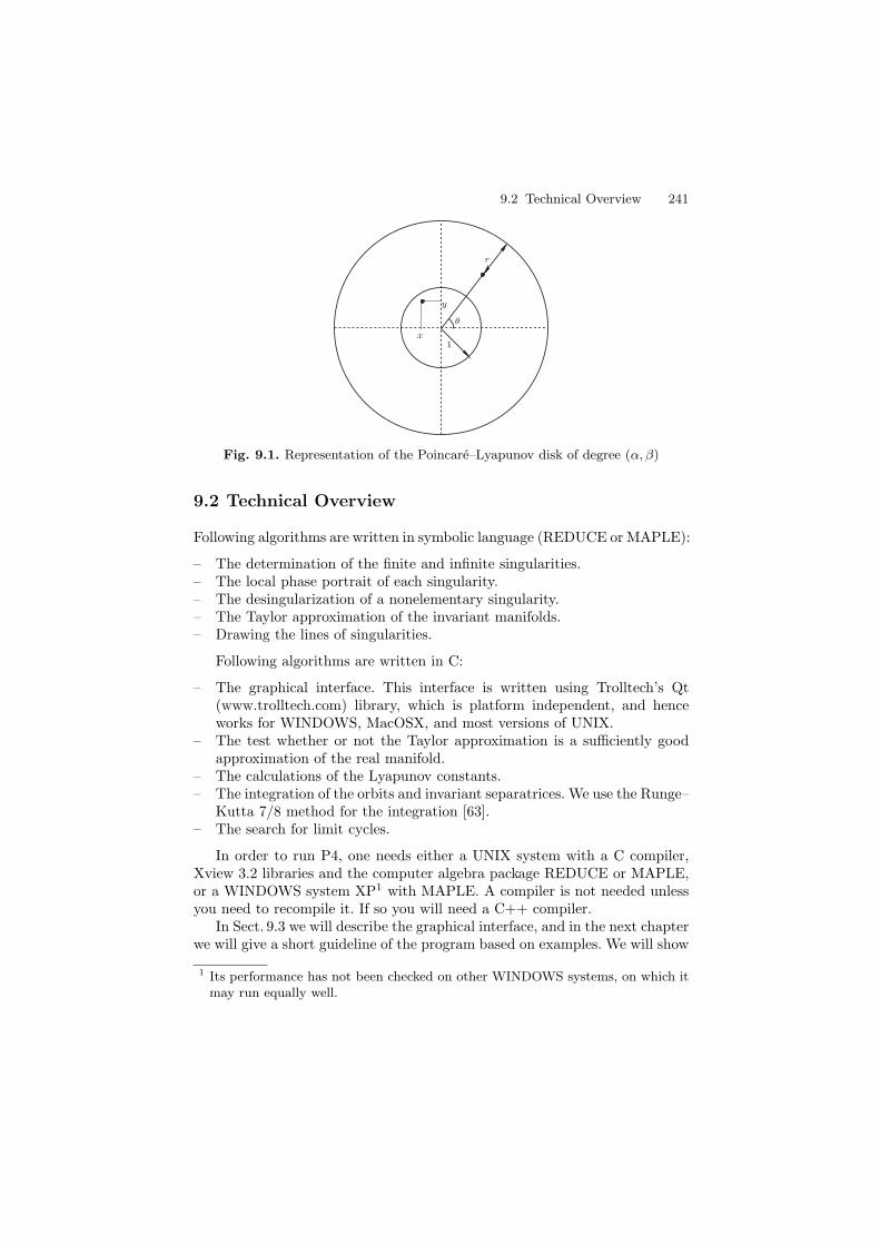
9.2 Technical Overview 241
r
y
x1
θ
Fig. 9.1. Representation of the Poincare–Lyapunov disk of degree (α, β)
9.2 Technical Overview
Following algorithms are written in symbolic language (REDUCE or MAPLE):
– The determination of the finite and infinite singularities.– The local phase portrait of each singularity.– The desingularization of a nonelementary singularity.– The Taylor approximation of the invariant manifolds.– Drawing the lines of singularities.
Following algorithms are written in C:
– The graphical interface. This interface is written using Trolltech’s Qt(www.trolltech.com) library, which is platform independent, and henceworks for WINDOWS, MacOSX, and most versions of UNIX.
– The test whether or not the Taylor approximation is a sufficiently goodapproximation of the real manifold.
– The calculations of the Lyapunov constants.– The integration of the orbits and invariant separatrices. We use the Runge–
Kutta 7/8 method for the integration [63].– The search for limit cycles.
In order to run P4, one needs either a UNIX system with a C compiler,Xview 3.2 libraries and the computer algebra package REDUCE or MAPLE,or a WINDOWS system XP1 with MAPLE. A compiler is not needed unlessyou need to recompile it. If so you will need a C++ compiler.
In Sect. 9.3 we will describe the graphical interface, and in the next chapterwe will give a short guideline of the program based on examples. We will show
1 Its performance has not been checked on other WINDOWS systems, on which itmay run equally well.
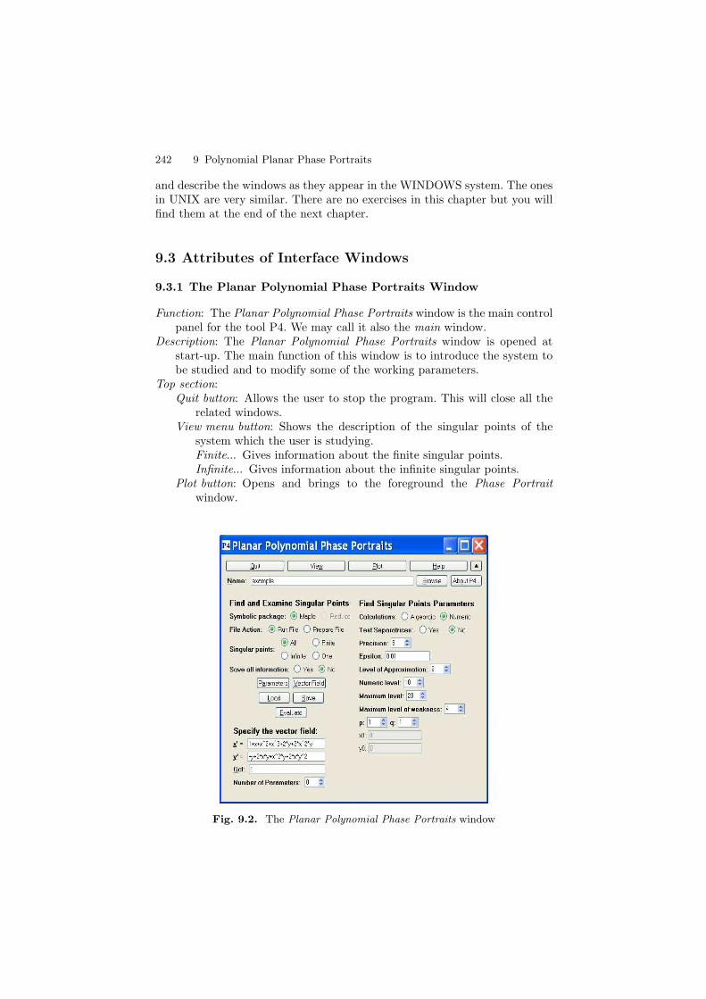
242 9 Polynomial Planar Phase Portraits
and describe the windows as they appear in the WINDOWS system. The onesin UNIX are very similar. There are no exercises in this chapter but you willfind them at the end of the next chapter.
9.3 Attributes of Interface Windows
9.3.1 The Planar Polynomial Phase Portraits Window
Function: The Planar Polynomial Phase Portraits window is the main controlpanel for the tool P4. We may call it also the main window.
Description: The Planar Polynomial Phase Portraits window is opened atstart-up. The main function of this window is to introduce the system tobe studied and to modify some of the working parameters.
Top section:Quit button: Allows the user to stop the program. This will close all the
related windows.View menu button: Shows the description of the singular points of the
system which the user is studying.Finite... Gives information about the finite singular points.Infinite... Gives information about the infinite singular points.
Plot button: Opens and brings to the foreground the Phase Portraitwindow.
Fig. 9.2. The Planar Polynomial Phase Portraits window
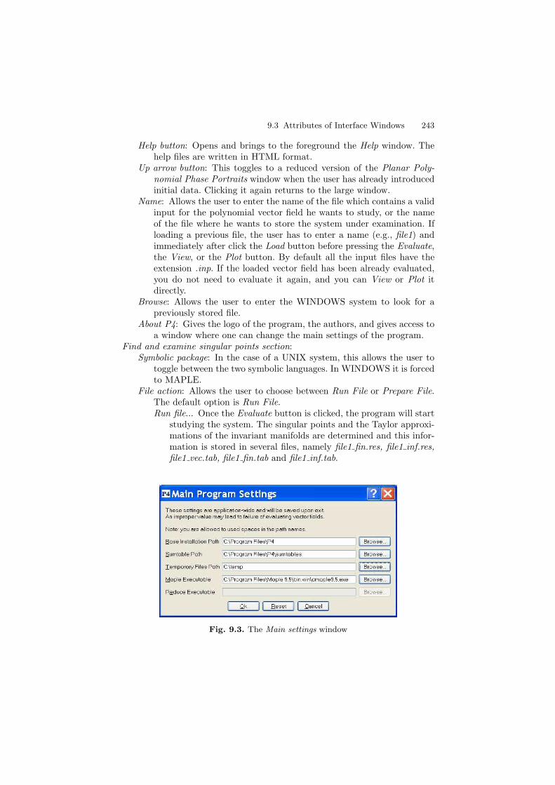
9.3 Attributes of Interface Windows 243
Help button: Opens and brings to the foreground the Help window. Thehelp files are written in HTML format.
Up arrow button: This toggles to a reduced version of the Planar Poly-nomial Phase Portraits window when the user has already introducedinitial data. Clicking it again returns to the large window.
Name: Allows the user to enter the name of the file which contains a validinput for the polynomial vector field he wants to study, or the nameof the file where he wants to store the system under examination. Ifloading a previous file, the user has to enter a name (e.g., file1) andimmediately after click the Load button before pressing the Evaluate,the View, or the Plot button. By default all the input files have theextension .inp. If the loaded vector field has been already evaluated,you do not need to evaluate it again, and you can View or Plot itdirectly.
Browse: Allows the user to enter the WINDOWS system to look for apreviously stored file.
About P4: Gives the logo of the program, the authors, and gives access toa window where one can change the main settings of the program.
Find and examine singular points section:Symbolic package: In the case of a UNIX system, this allows the user to
toggle between the two symbolic languages. In WINDOWS it is forcedto MAPLE.
File action: Allows the user to choose between Run File or Prepare File.The default option is Run File.Run file... Once the Evaluate button is clicked, the program will start
studying the system. The singular points and the Taylor approxi-mations of the invariant manifolds are determined and this infor-mation is stored in several files, namely file1 fin.res, file1 inf.res,file1 vec.tab, file1 fin.tab and file1 inf.tab.
Fig. 9.3. The Main settings window
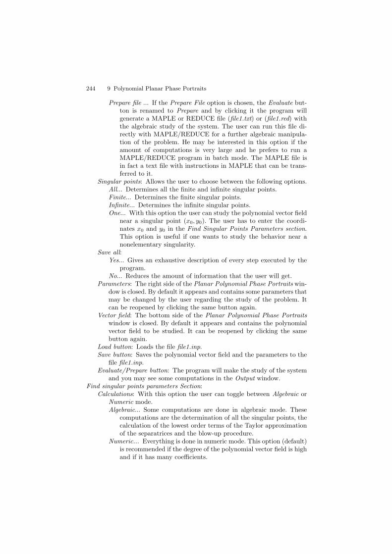
244 9 Polynomial Planar Phase Portraits
Prepare file ... If the Prepare File option is chosen, the Evaluate but-ton is renamed to Prepare and by clicking it the program willgenerate a MAPLE or REDUCE file (file1.txt) or (file1.red) withthe algebraic study of the system. The user can run this file di-rectly with MAPLE/REDUCE for a further algebraic manipula-tion of the problem. He may be interested in this option if theamount of computations is very large and he prefers to run aMAPLE/REDUCE program in batch mode. The MAPLE file isin fact a text file with instructions in MAPLE that can be trans-ferred to it.
Singular points: Allows the user to choose between the following options.All... Determines all the finite and infinite singular points.Finite... Determines the finite singular points.Infinite... Determines the infinite singular points.One... With this option the user can study the polynomial vector field
near a singular point (x0, y0). The user has to enter the coordi-nates x0 and y0 in the Find Singular Points Parameters section.This option is useful if one wants to study the behavior near anonelementary singularity.
Save all:Yes... Gives an exhaustive description of every step executed by the
program.No... Reduces the amount of information that the user will get.
Parameters: The right side of the Planar Polynomial Phase Portraits win-dow is closed. By default it appears and contains some parameters thatmay be changed by the user regarding the study of the problem. Itcan be reopened by clicking the same button again.
Vector field: The bottom side of the Planar Polynomial Phase Portraitswindow is closed. By default it appears and contains the polynomialvector field to be studied. It can be reopened by clicking the samebutton again.
Load button: Loads the file file1.inp.Save button: Saves the polynomial vector field and the parameters to the
file file1.inp.Evaluate/Prepare button: The program will make the study of the system
and you may see some computations in the Output window.Find singular points parameters Section:
Calculations: With this option the user can toggle between Algebraic orNumeric mode.Algebraic... Some computations are done in algebraic mode. These
computations are the determination of all the singular points, thecalculation of the lowest order terms of the Taylor approximationof the separatrices and the blow-up procedure.
Numeric... Everything is done in numeric mode. This option (default)is recommended if the degree of the polynomial vector field is highand if it has many coefficients.

9.3 Attributes of Interface Windows 245
Fig. 9.4. The Output window
Test separatrices: With this option the user can decide whether or not P4has to test every Taylor approximation of the separatrices. In generalit is recommended to set this option to Yes, but if the user has aspecific system from which he knows it has a separatrix which is hardto deal with, he may deactivate this option.
Precision: Here the user needs to define a precision to avoid roundingerrors. It tells the program to set a number a equal to zero if |a| < 10−δ
where δ is the Precision parameter. Of course, this means that itis possible that a nonzero number be considered equal to zero. Insuch cases the Precision has to be modified. The program makes allcomputations with 16 digits, so it is recommended that the value forPrecision be kept between 7 and 12.
Epsilon: In order to start integrating the separatrices we take an initialpoint at a certain distance Epsilon away from the singularity. Thisvalue is the default one we will use for every separatrix.
Level of approximation: Allows the user to set the order of the Taylorapproximation for the separatrices. If the option Test Separatrices isactivated, then P4 will test whether or not the Taylor approximation isa sufficiency good approximation of the real manifold (or separatrix).In case it is not, P4 computes the Taylor approximation one orderhigher and repeats the test again until the maximum degree is reachedor until the Taylor approximation is a sufficiency good approximationof the real manifold.
Numeric level: If the option Calculations is set to Algebraic, then the com-putation of the coefficients of the Taylor approximation will be donein Algebraic mode until the value in Numeric level is reached. Fromthis stage the computation will be done in Numeric mode.
Maximum level: Gives the maximum order of the Taylor approximation.If the test fails up to this level, then this will be explained in thereport that P4 will produce.
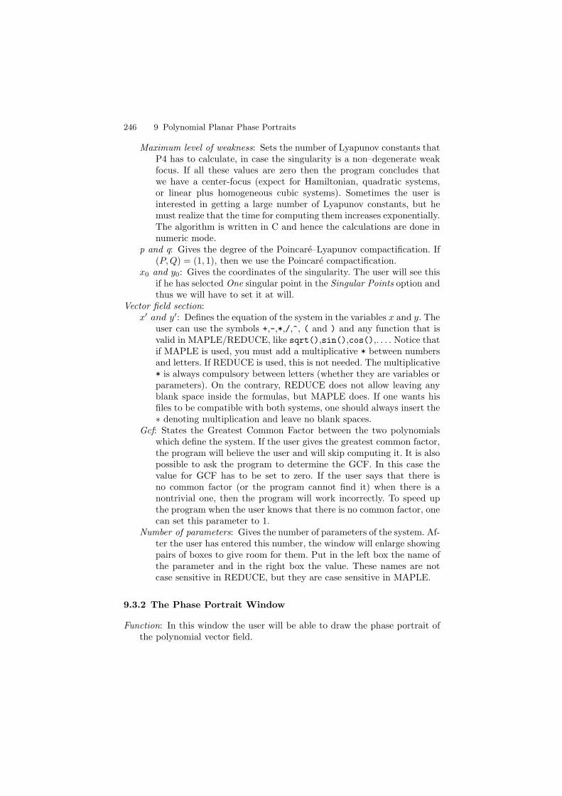
246 9 Polynomial Planar Phase Portraits
Maximum level of weakness: Sets the number of Lyapunov constants thatP4 has to calculate, in case the singularity is a non–degenerate weakfocus. If all these values are zero then the program concludes thatwe have a center-focus (expect for Hamiltonian, quadratic systems,or linear plus homogeneous cubic systems). Sometimes the user isinterested in getting a large number of Lyapunov constants, but hemust realize that the time for computing them increases exponentially.The algorithm is written in C and hence the calculations are done innumeric mode.
p and q: Gives the degree of the Poincare–Lyapunov compactification. If(P,Q) = (1, 1), then we use the Poincare compactification.
x0 and y0: Gives the coordinates of the singularity. The user will see thisif he has selected One singular point in the Singular Points option andthus we will have to set it at will.
Vector field section:x′ and y′: Defines the equation of the system in the variables x and y. The
user can use the symbols +,-,*,/,^, ( and ) and any function that isvalid in MAPLE/REDUCE, like sqrt(),sin(),cos(),. . . . Notice thatif MAPLE is used, you must add a multiplicative * between numbersand letters. If REDUCE is used, this is not needed. The multiplicative* is always compulsory between letters (whether they are variables orparameters). On the contrary, REDUCE does not allow leaving anyblank space inside the formulas, but MAPLE does. If one wants hisfiles to be compatible with both systems, one should always insert the∗ denoting multiplication and leave no blank spaces.
Gcf: States the Greatest Common Factor between the two polynomialswhich define the system. If the user gives the greatest common factor,the program will believe the user and will skip computing it. It is alsopossible to ask the program to determine the GCF. In this case thevalue for GCF has to be set to zero. If the user says that there isno common factor (or the program cannot find it) when there is anontrivial one, then the program will work incorrectly. To speed upthe program when the user knows that there is no common factor, onecan set this parameter to 1.
Number of parameters: Gives the number of parameters of the system. Af-ter the user has entered this number, the window will enlarge showingpairs of boxes to give room for them. Put in the left box the name ofthe parameter and in the right box the value. These names are notcase sensitive in REDUCE, but they are case sensitive in MAPLE.
9.3.2 The Phase Portrait Window
Function: In this window the user will be able to draw the phase portrait ofthe polynomial vector field.

9.3 Attributes of Interface Windows 247
Fig. 9.5. The Poincare Disc window
Description: This window is opened by selecting the Plot button in the Pla-nar Polynomial Phase Portraits window. The user will see the window asin Fig. 9.5. In this window there is a circle representing infinity and somesymbols representing the finite and infinite singular points of the system.If one presses the Legend button, the explanation of these symbols willappear.If (P,Q) �= (1, 1), then the Poincare–Lyapunov compactification is shown.In this case the user will see two circles. In the inner circle all the finitesingular points with modulus less than one are plotted. If the modulus ofa certain singular point is greater than one, then this point is plotted inthe annulus limited by the circle of radius one and the circle at infinity.If the option Singular Points is set to One, then the user will see a planarrepresentation of the neighborhood of such a point.

248 9 Polynomial Planar Phase Portraits
If the user moves the mouse in the drawing canvas, the current coordinatesof the mouse position are displayed in the window’s panel. If he studiesthe system on a Poincare or Poincare–Lyapunov disk, this region is blankwhen the mouse does not point to a region within the disk.The user can always enlarge or reduce this window as usual and an As-pect Ratio value will be shown on the bottom line to remind the user ifproportion holds (Aspect Ratio= 1) or not (Aspect Ratio �= 1).Mouse events in the main drawing canvas have the following effects:
– Clicking the LEFT button in the drawing canvas will select that pointand opens the Orbits window.
– Clicking the LEFT button while holding down the SHIFT key willselect the nearest singular point having separatrices (finite or infinite)and opens the Plot Separatrices window. You will see flashes aroundthe selected singular point.
– Clicking the LEFT button while holding down the CONTROL keycreates a rectangle used to make a zoom of a portion of the picture.You must move from one corner of the rectangular region to the oppo-site while holding both the LEFT button and the CONTROL KEY.Now the Phase Portrait - Zoom window will appear. At any time it ispossible to cancel the zoom by clicking on the RIGHT button.
Panel items:Close button: Closes this window and all the related windows.Refresh button: Clears the window and redraws the drawing canvas. This
is useful if all the separatrices are drawn, because the redraw will bringup the singularities which may have be shadowed by the lines.
Legend button: Opens and brings up to the foreground the Legend window.Orbits button: Opens and brings up to the foreground the Orbits window.
Fig. 9.6. The Legend window
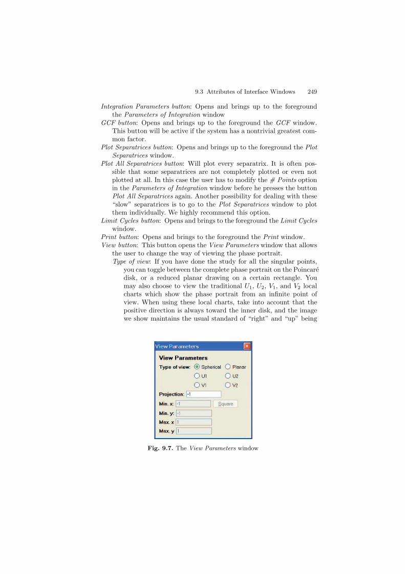
9.3 Attributes of Interface Windows 249
Integration Parameters button: Opens and brings up to the foregroundthe Parameters of Integration window
GCF button: Opens and brings up to the foreground the GCF window.This button will be active if the system has a nontrivial greatest com-mon factor.
Plot Separatrices button: Opens and brings up to the foreground the PlotSeparatrices window.
Plot All Separatrices button: Will plot every separatrix. It is often pos-sible that some separatrices are not completely plotted or even notplotted at all. In this case the user has to modify the # Points optionin the Parameters of Integration window before he presses the buttonPlot All Separatrices again. Another possibility for dealing with these“slow” separatrices is to go to the Plot Separatrices window to plotthem individually. We highly recommend this option.
Limit Cycles button: Opens and brings to the foreground the Limit Cycleswindow.
Print button: Opens and brings to the foreground the Print window.View button: This button opens the View Parameters window that allows
the user to change the way of viewing the phase portrait.Type of view: If you have done the study for all the singular points,
you can toggle between the complete phase portrait on the Poincaredisk, or a reduced planar drawing on a certain rectangle. Youmay also choose to view the traditional U1, U2, V1, and V2 localcharts which show the phase portrait from an infinite point ofview. When using these local charts, take into account that thepositive direction is always toward the inner disk, and the imagewe show maintains the usual standard of “right” and “up” being
Fig. 9.7. The View Parameters window

250 9 Polynomial Planar Phase Portraits
Fig. 9.8. A planar plot
positive while “left” and “down” are negative. So looking to theU1 chart (right side) or to the U2 chart (up side) may look differ-ent (symmetrical) from what we see on the disk. However, lookingto the V1 chart (left side) or to the V2 chart (down side) givesthe equivalent image as on the disk. Moreover, these images onthe infinite local charts are not restricted to the upper half of thePoincare disk, but are completed also with the lower part, that is,what happens in the opposite local chart.
Projection: This option is activated if the system is studied on aPoincare disk. It represents the z coordinate of the projectionpoint (0, 0, z) from which we project the points from the Poincaresphere to the Poincare disk. This value has to be negative. If theuser wants a parallel projection then he has to set this value tozero. The drawing canvas is refreshed after the user selects theRefresh button.
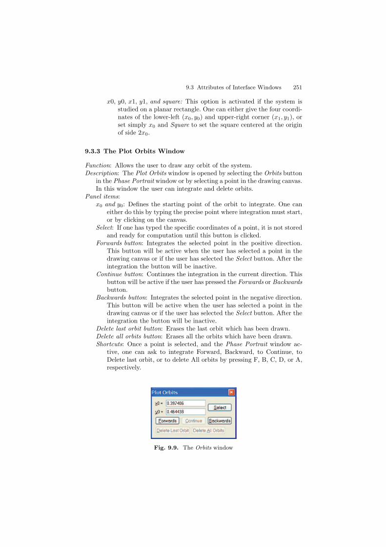
9.3 Attributes of Interface Windows 251
x0, y0, x1, y1, and square: This option is activated if the system isstudied on a planar rectangle. One can either give the four coordi-nates of the lower-left (x0, y0) and upper-right corner (x1, y1), orset simply x0 and Square to set the square centered at the originof side 2x0.
9.3.3 The Plot Orbits Window
Function: Allows the user to draw any orbit of the system.Description: The Plot Orbits window is opened by selecting the Orbits button
in the Phase Portrait window or by selecting a point in the drawing canvas.In this window the user can integrate and delete orbits.
Panel items:x0 and y0: Defines the starting point of the orbit to integrate. One can
either do this by typing the precise point where integration must start,or by clicking on the canvas.
Select: If one has typed the specific coordinates of a point, it is not storedand ready for computation until this button is clicked.
Forwards button: Integrates the selected point in the positive direction.This button will be active when the user has selected a point in thedrawing canvas or if the user has selected the Select button. After theintegration the button will be inactive.
Continue button: Continues the integration in the current direction. Thisbutton will be active if the user has pressed the Forwards or Backwardsbutton.
Backwards button: Integrates the selected point in the negative direction.This button will be active when the user has selected a point in thedrawing canvas or if the user has selected the Select button. After theintegration the button will be inactive.
Delete last orbit button: Erases the last orbit which has been drawn.Delete all orbits button: Erases all the orbits which have been drawn.Shortcuts: Once a point is selected, and the Phase Portrait window ac-
tive, one can ask to integrate Forward, Backward, to Continue, toDelete last orbit, or to delete All orbits by pressing F, B, C, D, or A,respectively.
Fig. 9.9. The Orbits window
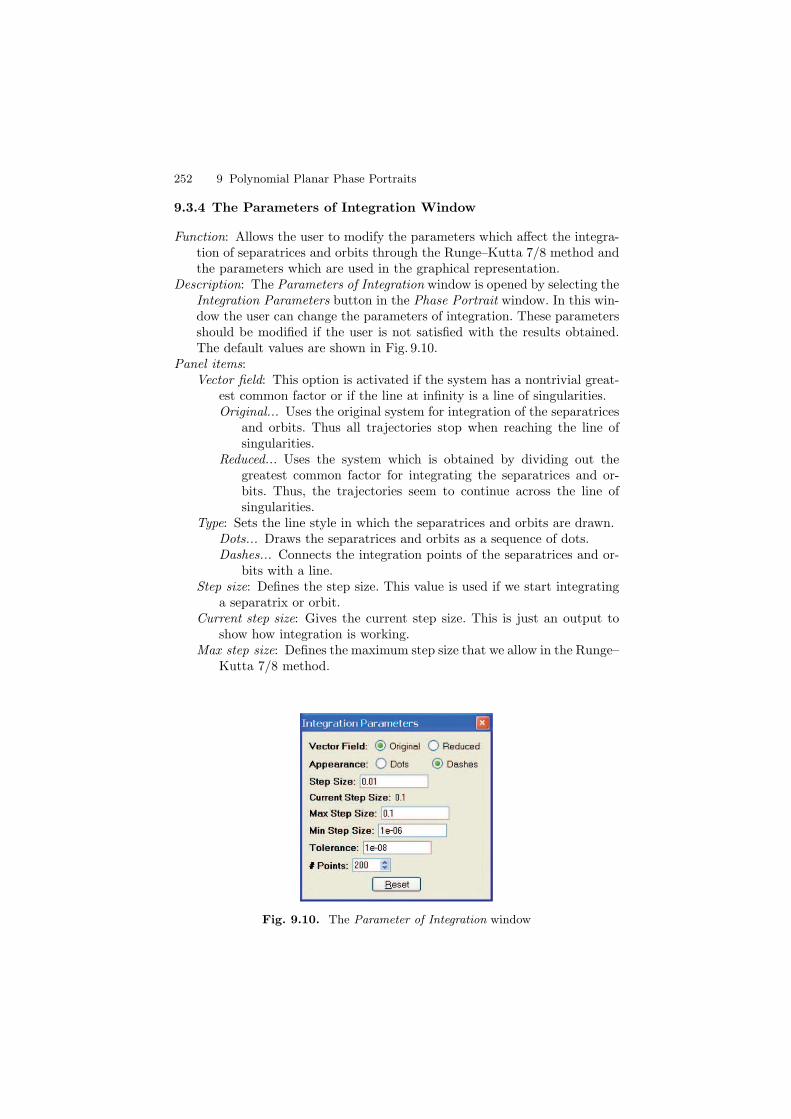
252 9 Polynomial Planar Phase Portraits
9.3.4 The Parameters of Integration Window
Function: Allows the user to modify the parameters which affect the integra-tion of separatrices and orbits through the Runge–Kutta 7/8 method andthe parameters which are used in the graphical representation.
Description: The Parameters of Integration window is opened by selecting theIntegration Parameters button in the Phase Portrait window. In this win-dow the user can change the parameters of integration. These parametersshould be modified if the user is not satisfied with the results obtained.The default values are shown in Fig. 9.10.
Panel items:Vector field: This option is activated if the system has a nontrivial great-
est common factor or if the line at infinity is a line of singularities.Original... Uses the original system for integration of the separatrices
and orbits. Thus all trajectories stop when reaching the line ofsingularities.
Reduced... Uses the system which is obtained by dividing out thegreatest common factor for integrating the separatrices and or-bits. Thus, the trajectories seem to continue across the line ofsingularities.
Type: Sets the line style in which the separatrices and orbits are drawn.Dots... Draws the separatrices and orbits as a sequence of dots.Dashes... Connects the integration points of the separatrices and or-
bits with a line.Step size: Defines the step size. This value is used if we start integrating
a separatrix or orbit.Current step size: Gives the current step size. This is just an output to
show how integration is working.Max step size: Defines the maximum step size that we allow in the Runge–
Kutta 7/8 method.
Fig. 9.10. The Parameter of Integration window
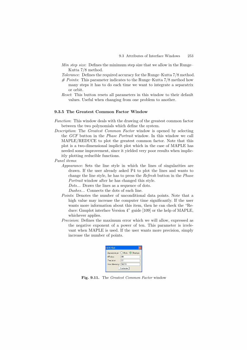
9.3 Attributes of Interface Windows 253
Min step size: Defines the minimum step size that we allow in the Runge–Kutta 7/8 method.
Tolerance: Defines the required accuracy for the Runge–Kutta 7/8 method.# Points: This parameter indicates to the Runge–Kutta 7/8 method how
many steps it has to do each time we want to integrate a separatrixor orbit.
Reset: This button resets all parameters in this window to their defaultvalues. Useful when changing from one problem to another.
9.3.5 The Greatest Common Factor Window
Function: This window deals with the drawing of the greatest common factorbetween the two polynomials which define the system.
Description: The Greatest Common Factor window is opened by selectingthe GCF button in the Phase Portrait window. In this window we callMAPLE/REDUCE to plot the greatest common factor. Note that thisplot is a two-dimensional implicit plot which in the case of MAPLE hasneeded some improvement, since it yielded very poor results when implic-itly plotting reducible functions.
Panel items:Appearance: Sets the line style in which the lines of singularities are
drawn. If the user already asked P4 to plot the lines and wants tochange the line style, he has to press the Refresh button in the PhasePortrait window after he has changed this style.Dots... Draws the lines as a sequence of dots.Dashes... Connects the dots of each line.
Points: Denotes the number of unconditional data points. Note that ahigh value may increase the computer time significantly. If the userwants more information about this item, then he can check the “Re-duce: Gnuplot interface Version 4” guide [109] or the help of MAPLE,whichever applies.
Precision: Defines the maximum error which we will allow, expressed asthe negative exponent of a power of ten. This parameter is irrele-vant when MAPLE is used. If the user wants more precision, simplyincrease the number of points.
Fig. 9.11. The Greatest Common Factor window
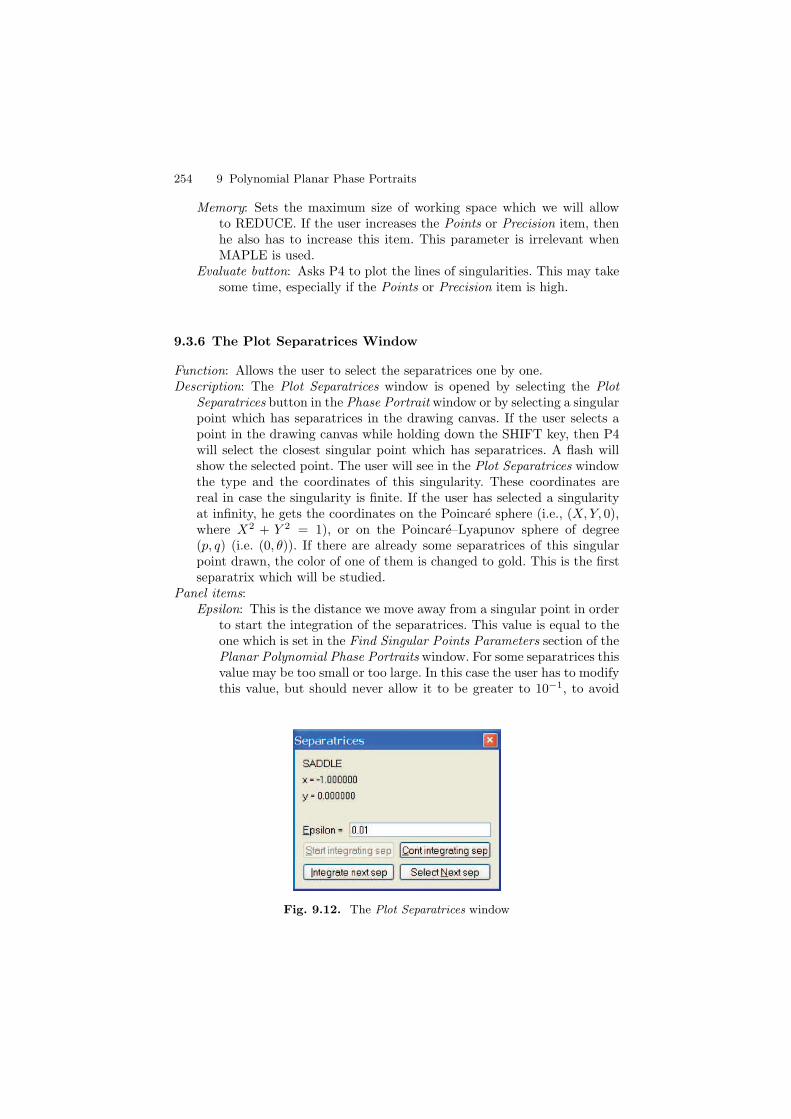
254 9 Polynomial Planar Phase Portraits
Memory: Sets the maximum size of working space which we will allowto REDUCE. If the user increases the Points or Precision item, thenhe also has to increase this item. This parameter is irrelevant whenMAPLE is used.
Evaluate button: Asks P4 to plot the lines of singularities. This may takesome time, especially if the Points or Precision item is high.
9.3.6 The Plot Separatrices Window
Function: Allows the user to select the separatrices one by one.Description: The Plot Separatrices window is opened by selecting the Plot
Separatrices button in the Phase Portrait window or by selecting a singularpoint which has separatrices in the drawing canvas. If the user selects apoint in the drawing canvas while holding down the SHIFT key, then P4will select the closest singular point which has separatrices. A flash willshow the selected point. The user will see in the Plot Separatrices windowthe type and the coordinates of this singularity. These coordinates arereal in case the singularity is finite. If the user has selected a singularityat infinity, he gets the coordinates on the Poincare sphere (i.e., (X,Y, 0),where X2 + Y 2 = 1), or on the Poincare–Lyapunov sphere of degree(p, q) (i.e. (0, θ)). If there are already some separatrices of this singularpoint drawn, the color of one of them is changed to gold. This is the firstseparatrix which will be studied.
Panel items:Epsilon: This is the distance we move away from a singular point in order
to start the integration of the separatrices. This value is equal to theone which is set in the Find Singular Points Parameters section of thePlanar Polynomial Phase Portraits window. For some separatrices thisvalue may be too small or too large. In this case the user has to modifythis value, but should never allow it to be greater to 10−1, to avoid
Fig. 9.12. The Plot Separatrices window

9.3 Attributes of Interface Windows 255
large errors when choosing the initial integration point. Do not forgetto press the RETURN button after changing this value.
Start Integrating Sep button: Starts the integration of the chosen separa-trix.
Cont Integrating Sep button: Continues the integration of the selectedseparatrix.
Integrate Next Sep button: Selects another separatrix of the same singularpoint and starts with the integration.
Select Next Sep button: It selects another separatrix of the same singularpoint.
9.3.7 The Limit Cycles Window
Function: Allows the user to search for non semistable limit cycles up to acertain degree of precision.
Description: The Limit Cycles window is opened by selecting the Limit Cyclesbutton from the Phase Portrait window. In this window the user has togive two points forming a segment which he suspects is cut by at least onelimit cycle.
Panel items:x0, y0: Defines the first point of the line segment.x1, y1: Defines the last point of the line segment. The user can select
these two points by clicking the left button of the mouse on the firstpoint, and while holding the button down, moving the mouse to thesecond point and releasing the button.
Grid: Determines the precision up to which the limit cycles will be deter-mined. That is, if two consecutive limit cycles cut the selected segmentin two points at distance greater than the Grid value, then P4 will de-tect them. Otherwise, it is possible that not both limit cycles aredetected or that a continuum of limit cycles may be detected becauseof lack of precision.
# Points: This parameter equals the number of steps the Runge–Kutta7/8 method has to do each time we want to integrate an orbit withinitial condition a point of the segment. If the orbit does not cross the
Fig. 9.13. The Limit Cycles window
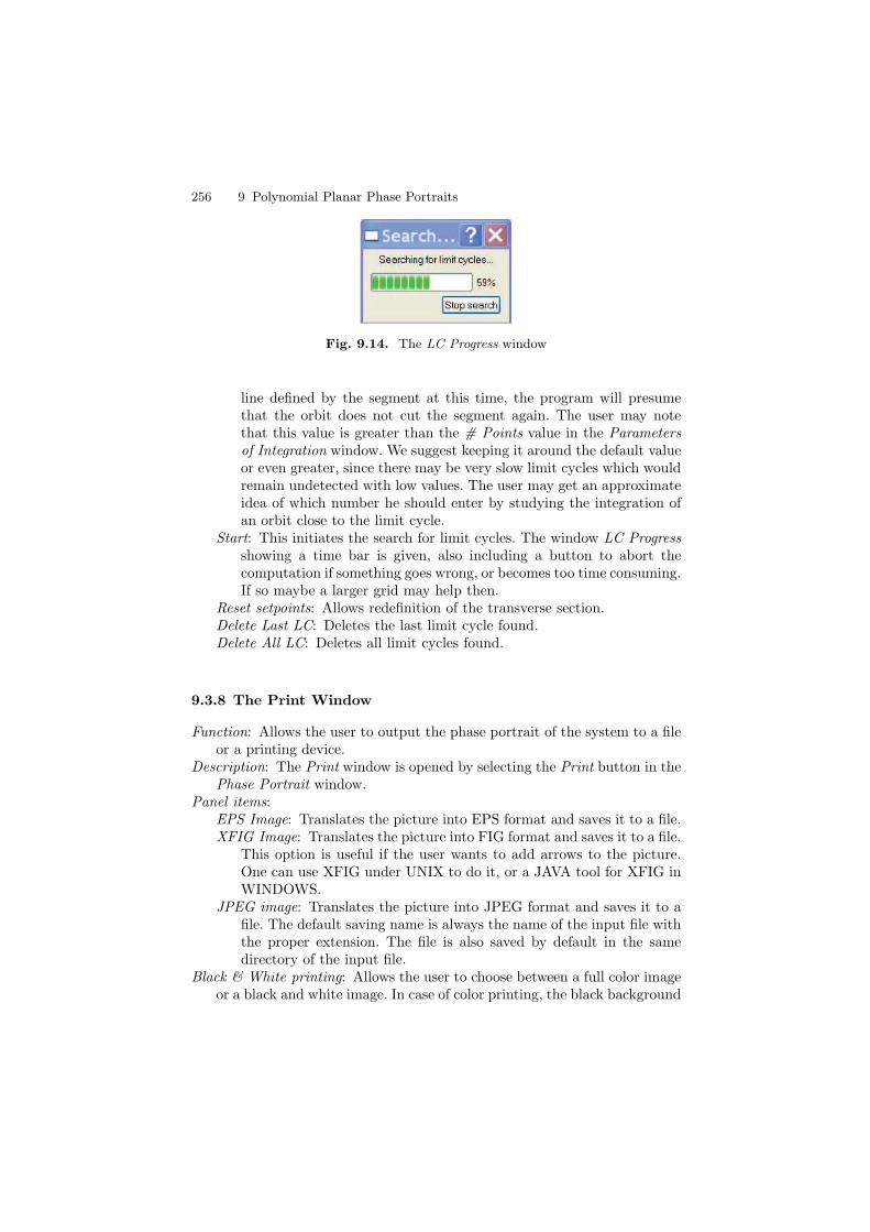
256 9 Polynomial Planar Phase Portraits
Fig. 9.14. The LC Progress window
line defined by the segment at this time, the program will presumethat the orbit does not cut the segment again. The user may notethat this value is greater than the # Points value in the Parametersof Integration window. We suggest keeping it around the default valueor even greater, since there may be very slow limit cycles which wouldremain undetected with low values. The user may get an approximateidea of which number he should enter by studying the integration ofan orbit close to the limit cycle.
Start: This initiates the search for limit cycles. The window LC Progressshowing a time bar is given, also including a button to abort thecomputation if something goes wrong, or becomes too time consuming.If so maybe a larger grid may help then.
Reset setpoints: Allows redefinition of the transverse section.Delete Last LC: Deletes the last limit cycle found.Delete All LC: Deletes all limit cycles found.
9.3.8 The Print Window
Function: Allows the user to output the phase portrait of the system to a fileor a printing device.
Description: The Print window is opened by selecting the Print button in thePhase Portrait window.
Panel items:EPS Image: Translates the picture into EPS format and saves it to a file.XFIG Image: Translates the picture into FIG format and saves it to a file.
This option is useful if the user wants to add arrows to the picture.One can use XFIG under UNIX to do it, or a JAVA tool for XFIG inWINDOWS.
JPEG image: Translates the picture into JPEG format and saves it to afile. The default saving name is always the name of the input file withthe proper extension. The file is also saved by default in the samedirectory of the input file.
Black & White printing: Allows the user to choose between a full color imageor a black and white image. In case of color printing, the black background

9.3 Attributes of Interface Windows 257
Fig. 9.15. The Print window
is turned into white, while the white line at infinity and the yellow orbitsare turned into black and other colors are left unchanged. In case of Black& White, background is white and all drawing is in black.
Cancel button: Cancels everything and closes the window.Output resolution (in DPI): All images are produced 15 cm wide, so if the
user needs a bigger picture, it is suggested that he increases the Outputresolution so as to maintain quality after rescaling the picture with someother tool.
Line with (in mm): The higher, the wider.Symbol size (in mm): The higher, the larger.


10
Examples for Running P4
In this chapter we are going to provide several examples about the use of P4[9], moving from easy examples to more complex ones, and trying to produceall the different situations and the most tricky problems that we have met upto now. Of course, we cannot pretend to cover all possible situations that mayappear, since we are not aware of the complexity of the problem the readermay try to study, but at least we hope to give enough clues about how tosolve them, or to show the impossibility of getting the complete study.
For these examples we will use the program running on a WINDOWSsystem, and using MAPLE as symbolic language. Where something differentis expected for REDUCE’s users, it will be described.
10.1 Some Basic Examples
Example 10.1 Consider the cubic vector field
x = y − x3,
y = x + y + y3.(10.1)
The first thing to do after starting P4 is to introduce system (10.1) to theprogram. First you provide a name for the system such as, e.g., example1.
At the bottom of the window you see two fields where you can introducethe equation of the vector field. In the x’ field you type y-x^3 and in they’ field x+y+y^3. Since there is no line of singularities, you can leave theGcf field equal to 1. Now you are ready to study the system. Simply pressthe Evaluate button. The program now calls MAPLE (or REDUCE) whichdetermines the singular points. You have to wait until you see in the Outputwindow a message as in Fig. 10.1, or simply check that the button Evaluatehas become active again.
Go to the top of the window and press the View menu button with theleft button of the mouse. This will open a menu where you can choose to see
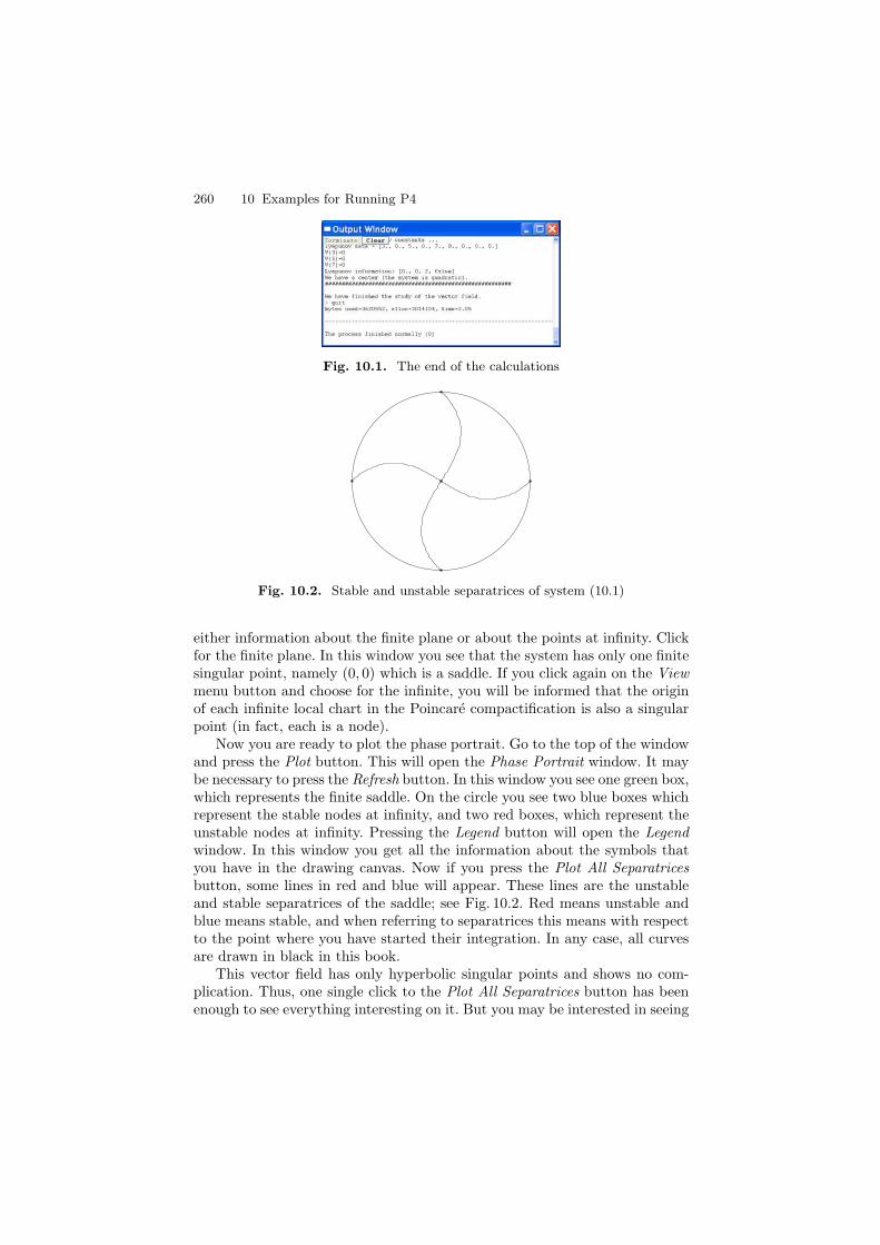
260 10 Examples for Running P4
Fig. 10.1. The end of the calculations
Fig. 10.2. Stable and unstable separatrices of system (10.1)
either information about the finite plane or about the points at infinity. Clickfor the finite plane. In this window you see that the system has only one finitesingular point, namely (0, 0) which is a saddle. If you click again on the Viewmenu button and choose for the infinite, you will be informed that the originof each infinite local chart in the Poincare compactification is also a singularpoint (in fact, each is a node).
Now you are ready to plot the phase portrait. Go to the top of the windowand press the Plot button. This will open the Phase Portrait window. It maybe necessary to press the Refresh button. In this window you see one green box,which represents the finite saddle. On the circle you see two blue boxes whichrepresent the stable nodes at infinity, and two red boxes, which represent theunstable nodes at infinity. Pressing the Legend button will open the Legendwindow. In this window you get all the information about the symbols thatyou have in the drawing canvas. Now if you press the Plot All Separatricesbutton, some lines in red and blue will appear. These lines are the unstableand stable separatrices of the saddle; see Fig. 10.2. Red means unstable andblue means stable, and when referring to separatrices this means with respectto the point where you have started their integration. In any case, all curvesare drawn in black in this book.
This vector field has only hyperbolic singular points and shows no com-plication. Thus, one single click to the Plot All Separatrices button has beenenough to see everything interesting on it. But you may be interested in seeing
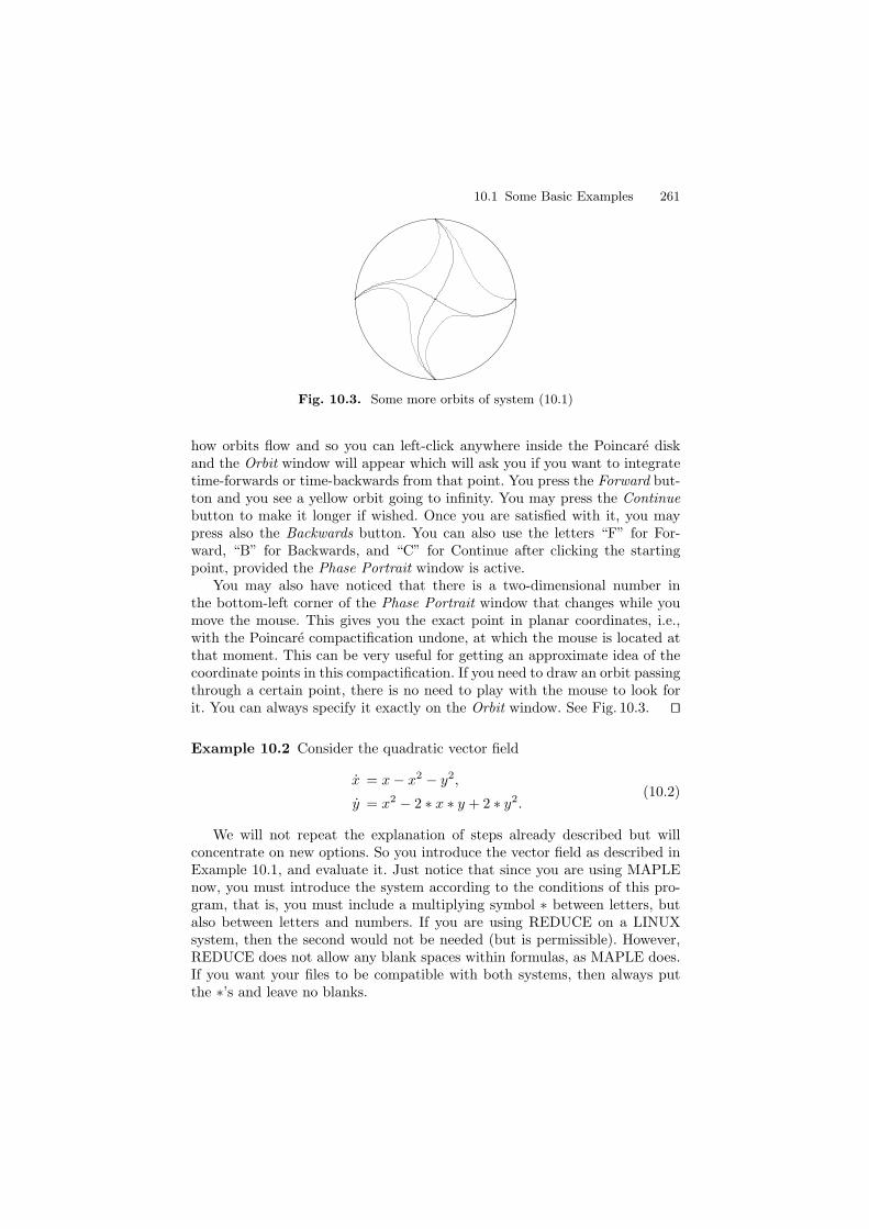
10.1 Some Basic Examples 261
Fig. 10.3. Some more orbits of system (10.1)
how orbits flow and so you can left-click anywhere inside the Poincare diskand the Orbit window will appear which will ask you if you want to integratetime-forwards or time-backwards from that point. You press the Forward but-ton and you see a yellow orbit going to infinity. You may press the Continuebutton to make it longer if wished. Once you are satisfied with it, you maypress also the Backwards button. You can also use the letters “F” for For-ward, “B” for Backwards, and “C” for Continue after clicking the startingpoint, provided the Phase Portrait window is active.
You may also have noticed that there is a two-dimensional number inthe bottom-left corner of the Phase Portrait window that changes while youmove the mouse. This gives you the exact point in planar coordinates, i.e.,with the Poincare compactification undone, at which the mouse is located atthat moment. This can be very useful for getting an approximate idea of thecoordinate points in this compactification. If you need to draw an orbit passingthrough a certain point, there is no need to play with the mouse to look forit. You can always specify it exactly on the Orbit window. See Fig. 10.3. ⊓⊔
Example 10.2 Consider the quadratic vector field
x = x − x2 − y2,
y = x2 − 2 ∗ x ∗ y + 2 ∗ y2.(10.2)
We will not repeat the explanation of steps already described but willconcentrate on new options. So you introduce the vector field as described inExample 10.1, and evaluate it. Just notice that since you are using MAPLEnow, you must introduce the system according to the conditions of this pro-gram, that is, you must include a multiplying symbol ∗ between letters, butalso between letters and numbers. If you are using REDUCE on a LINUXsystem, then the second would not be needed (but is permissible). However,REDUCE does not allow any blank spaces within formulas, as MAPLE does.If you want your files to be compatible with both systems, then always putthe ∗’s and leave no blanks.
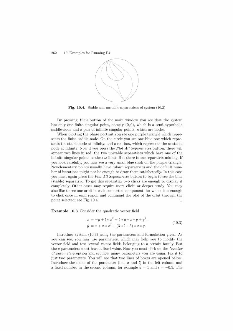
262 10 Examples for Running P4
Fig. 10.4. Stable and unstable separatrices of system (10.2)
By pressing View button of the main window you see that the systemhas only one finite singular point, namely (0, 0), which is a semi-hyperbolicsaddle-node and a pair of infinite singular points, which are nodes.
When plotting the phase portrait you see one purple triangle which repre-sents the finite saddle-node. On the circle you see one blue box which repre-sents the stable node at infinity, and a red box, which represents the unstablenode at infinity. Now if you press the Plot All Separatrices button, there willappear two lines in red, the two unstable separatices which have one of theinfinite singular points as their ω-limit. But there is one separatrix missing. Ifyou look carefully, you may see a very small blue slash on the purple triangle.Nonelementary points usually have “slow” separatrices and the default num-ber of iterations might not be enough to draw them satisfactorily. In this caseyou must again press the Plot All Separatrices button to begin to see the blue(stable) separatrix. To get this separatrix two clicks are enough to display itcompletely. Other cases may require more clicks or deeper study. You mayalso like to see one orbit in each connected component, for which it is enoughto click once in each region and command the plot of the orbit through thepoint selected; see Fig. 10.4. ⊓⊔
Example 10.3 Consider the quadratic vector field
x = −y + l ∗ x2 + 5 ∗ a ∗ x ∗ y + y2,
y = x + a ∗ x2 + (3 ∗ l + 5) ∗ x ∗ y.(10.3)
Introduce system (10.3) using the parameters and formulation given. Asyou can see, you may use parameters, which may help you to modify thevector field and test several vector fields belonging to a certain family. Butthese parameters must have a fixed value. Now you must click on the Numberof parameters option and set how many parameters you are using. Fix it tojust two parameters. You will see that two lines of boxes are opened below.Introduce the name of the parameter (i.e., a and l) in the left column anda fixed number in the second column, for example a = 1 and l = −0.5. The
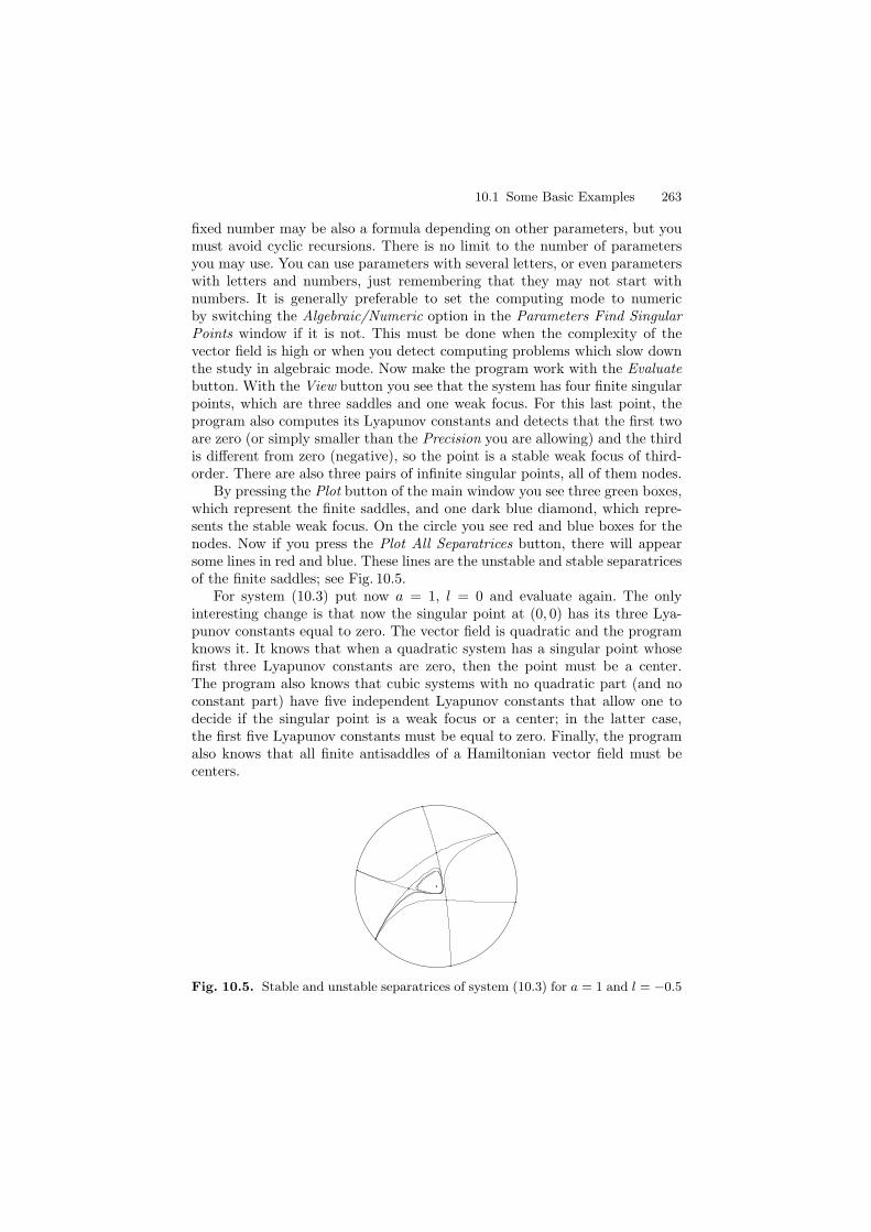
10.1 Some Basic Examples 263
fixed number may be also a formula depending on other parameters, but youmust avoid cyclic recursions. There is no limit to the number of parametersyou may use. You can use parameters with several letters, or even parameterswith letters and numbers, just remembering that they may not start withnumbers. It is generally preferable to set the computing mode to numericby switching the Algebraic/Numeric option in the Parameters Find SingularPoints window if it is not. This must be done when the complexity of thevector field is high or when you detect computing problems which slow downthe study in algebraic mode. Now make the program work with the Evaluatebutton. With the View button you see that the system has four finite singularpoints, which are three saddles and one weak focus. For this last point, theprogram also computes its Lyapunov constants and detects that the first twoare zero (or simply smaller than the Precision you are allowing) and the thirdis different from zero (negative), so the point is a stable weak focus of third-order. There are also three pairs of infinite singular points, all of them nodes.
By pressing the Plot button of the main window you see three green boxes,which represent the finite saddles, and one dark blue diamond, which repre-sents the stable weak focus. On the circle you see red and blue boxes for thenodes. Now if you press the Plot All Separatrices button, there will appearsome lines in red and blue. These lines are the unstable and stable separatricesof the finite saddles; see Fig. 10.5.
For system (10.3) put now a = 1, l = 0 and evaluate again. The onlyinteresting change is that now the singular point at (0, 0) has its three Lya-punov constants equal to zero. The vector field is quadratic and the programknows it. It knows that when a quadratic system has a singular point whosefirst three Lyapunov constants are zero, then the point must be a center.The program also knows that cubic systems with no quadratic part (and noconstant part) have five independent Lyapunov constants that allow one todecide if the singular point is a weak focus or a center; in the latter case,the first five Lyapunov constants must be equal to zero. Finally, the programalso knows that all finite antisaddles of a Hamiltonian vector field must becenters.
Fig. 10.5. Stable and unstable separatrices of system (10.3) for a = 1 and l = −0.5
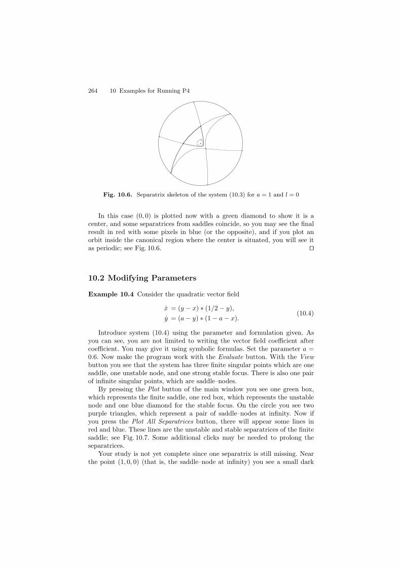
264 10 Examples for Running P4
Fig. 10.6. Separatrix skeleton of the system (10.3) for a = 1 and l = 0
In this case (0, 0) is plotted now with a green diamond to show it is acenter, and some separatrices from saddles coincide, so you may see the finalresult in red with some pixels in blue (or the opposite), and if you plot anorbit inside the canonical region where the center is situated, you will see itas periodic; see Fig. 10.6. ⊓⊔
10.2 Modifying Parameters
Example 10.4 Consider the quadratic vector field
x = (y − x) ∗ (1/2 − y),
y = (a − y) ∗ (1 − a − x).(10.4)
Introduce system (10.4) using the parameter and formulation given. Asyou can see, you are not limited to writing the vector field coefficient aftercoefficient. You may give it using symbolic formulas. Set the parameter a =0.6. Now make the program work with the Evaluate button. With the Viewbutton you see that the system has three finite singular points which are onesaddle, one unstable node, and one strong stable focus. There is also one pairof infinite singular points, which are saddle–nodes.
By pressing the Plot button of the main window you see one green box,which represents the finite saddle, one red box, which represents the unstablenode and one blue diamond for the stable focus. On the circle you see twopurple triangles, which represent a pair of saddle–nodes at infinity. Now ifyou press the Plot All Separatrices button, there will appear some lines inred and blue. These lines are the unstable and stable separatrices of the finitesaddle; see Fig. 10.7. Some additional clicks may be needed to prolong theseparatrices.
Your study is not yet complete since one separatrix is still missing. Nearthe point (1, 0, 0) (that is, the saddle–node at infinity) you see a small dark
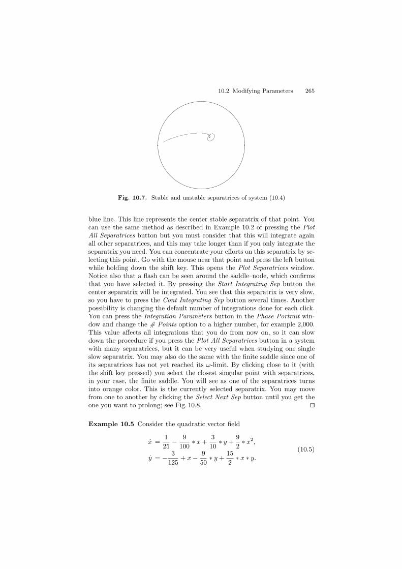
10.2 Modifying Parameters 265
Fig. 10.7. Stable and unstable separatrices of system (10.4)
blue line. This line represents the center stable separatrix of that point. Youcan use the same method as described in Example 10.2 of pressing the PlotAll Separatrices button but you must consider that this will integrate againall other separatrices, and this may take longer than if you only integrate theseparatrix you need. You can concentrate your efforts on this separatrix by se-lecting this point. Go with the mouse near that point and press the left buttonwhile holding down the shift key. This opens the Plot Separatrices window.Notice also that a flash can be seen around the saddle–node, which confirmsthat you have selected it. By pressing the Start Integrating Sep button thecenter separatrix will be integrated. You see that this separatrix is very slow,so you have to press the Cont Integrating Sep button several times. Anotherpossibility is changing the default number of integrations done for each click.You can press the Integration Parameters button in the Phase Portrait win-dow and change the # Points option to a higher number, for example 2,000.This value affects all integrations that you do from now on, so it can slowdown the procedure if you press the Plot All Separatrices button in a systemwith many separatrices, but it can be very useful when studying one singleslow separatrix. You may also do the same with the finite saddle since one ofits separatrices has not yet reached its ω-limit. By clicking close to it (withthe shift key pressed) you select the closest singular point with separatrices,in your case, the finite saddle. You will see as one of the separatrices turnsinto orange color. This is the currently selected separatrix. You may movefrom one to another by clicking the Select Next Sep button until you get theone you want to prolong; see Fig. 10.8. ⊓⊔
Example 10.5 Consider the quadratic vector field
x =1
25− 9
100∗ x +
3
10∗ y +
9
2∗ x2,
y = − 3
125+ x − 9
50∗ y +
15
2∗ x ∗ y.
(10.5)
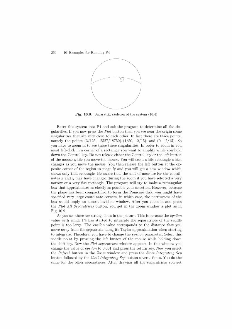
266 10 Examples for Running P4
Fig. 10.8. Separatrix skeleton of the system (10.4)
Enter this system into P4 and ask the program to determine all the sin-gularities. If you now press the Plot button then you see near the origin somesingularities that are very close to each other. In fact there are three points,namely the points (3/125,−2527/18750), (1/50,−2/15), and (0,−2/15). Soyou have to zoom in to see these three singularities. In order to zoom in youmust left-click in a corner of a rectangle you want to amplify while you holddown the Control key. Do not release either the Control key or the left buttonof the mouse while you move the mouse. You will see a white rectangle whichchanges as you move the mouse. You then release the left button at the op-posite corner of the region to magnify and you will get a new window whichshows only that rectangle. Be aware that the unit of measure for the coordi-nates x and y may have changed during the zoom if you have selected a verynarrow or a very flat rectangle. The program will try to make a rectangularbox that approximates as closely as possible your selection. However, becausethe plane has been compactified to form the Poincare disk, you might havespecified very large coordinate corners, in which case, the narrowness of thebox would imply an almost invisible window. After you zoom in and pressthe Plot All Separatrices button, you get in the zoom window a plot as inFig. 10.9.
As you see there are strange lines in the picture. This is because the epsilonvalue with which P4 has started to integrate the separatrices of the saddlepoint is too large. The epsilon value corresponds to the distance that youmove away from the separatrix along its Taylor approximation when startingto integrate. Therefore, you have to change the epsilon parameter. Select thissaddle point by pressing the left button of the mouse while holding downthe shift key. Now the Plot separatrices window appears. In this window youchange the value of epsilon to 0.001 and press the return key. Now you selectthe Refresh button in the Zoom window and press the Start Integrating Sepbutton followed by the Cont Integrating Sep button several times. You do thesame for the other separatrices. After drawing all the separatrices you get

10.2 Modifying Parameters 267
Fig. 10.9. Epsilon value too great
Fig. 10.10. Good epsilon value
Fig. 10.11. Phase portrait of system (10.5)
the picture of Fig. 10.10. To obtain a global vision of the phase portrait moreorbits have to be drawn; see Fig. 10.11.
There is also a global epsilon value which can be set in the Find SingularPoints Parameters section of the main window and that is used by defaultin all singular points with separatrices. This number is set by default to 0.01since lower values are needed only for very special cases and they would delay
268 10 Examples for Running P4
most other systems. Also, sometimes, and for some specific cases, it may benecessary to set epsilon to higher values, such as 0.05 or even 0.1, to help theprogram and start integrating further from the singular point, avoiding thelow start of some central manifolds. ⊓⊔Example 10.6 Consider the cubic vector field
x = y,
y = −x2 ∗ (x + 1) + d ∗ (a + b ∗ x + x2) ∗ y.(10.6)
Introduce system (10.6) using the parameters and formulation given. Youtest first the case d = 0.1, a = b = 0 and evaluate it in Numeric mode.With the View button you see that the system has two finite singular points,one strong unstable focus and one degenerate point at (0, 0). This point isstudied in detail and you see that the program informs you that it has a stableseparatrix arriving in the direction (x(t), y(t)) = (−t2, 0.8165t3 + . . .) and anunstable separatrix departing in the direction (x(t), y(t)) = (−t2,−0.8165t3 +. . .). It also tells you that the sector between the first and second separatrixis hyperbolic, and the sector between the last (second) and first separatrix isalso hyperbolic. It also gives you the index of the singular point, which is 0.Thus the point is a cusp. There are also two pairs of infinite singular points,one a semi-hyperbolic saddle and the other a degenerate point. For this lastpoint, the program has found four sectors but it happens that they are allparabolic. So the four separatrices described by the program are just orbitswhich arrive to that point but are not separatrices, even though it says so.In fact, the degenerate point is nothing more than a degenerate stable node.Only separatrices which coincide with separatrices of hyperbolic sectors arereal ones. Those which limit with parabolic or elliptic sectors are just localseparatrices in the blowing up system which may not maintain their characterin the global system.
By pressing the Plot button of the main window you see one red diamond,which represent the finite focus, and one cross which represents the cusp(in general any degenerate singular point). On the circle you see two greentriangles and two more crosses, which represent a pair of semi-hyperbolicsaddles and the degenerate singular points at infinity, respectively. Now if youpress the Plot All Separatrices button, there will appear some lines in red andblue starting at the cusp. Two more clicks on the same button give you abetter idea of what those separatrices do; see Fig. 10.12.
Your study is not yet complete since two separatrices are still missing. Theinfinite semi-hyperbolic saddles must have one separatrix each moving to thefinite plane, but the most that you can see are some unclear blue dashes atthe top and the bottom. If you zoom in on the topmost region as describedin Example 10.4, you will realize that the blue dash does not correspond tothe saddle, but it is one of the orbits of the degenerate node in which you arenot interested at all. So you must select the semi-hyperbolic saddle by left-clicking close to it while holding the shift key. This time, you must modify the

10.2 Modifying Parameters 269
Fig. 10.12. Stable and unstable separatrices of system (10.6) with d = 0.1 anda = b = 0
Fig. 10.13. Stepping too fast
epsilon to a greater value (like 0.1), but you must also modify the maximumintegration step size allowed in Phase Portrait–Integration Parameters windowgiven by Max Step Size. Try setting it to 10 and also setting # Points to 2,000.After pressing the Cont Integrating Sep two times you see it drawing, but whatappears does not seem to be a differentiable curve, but a dashed one, whichbecomes even worse if you continue integrating; see Fig. 10.13. The integrationspeed needed to get away from the singular point is too fast when you are farfrom it.
You need to play with the parameters in order to get a nice phase portrait.For example, click on the Epsilon box of the Separatrices window and press re-turn to redraw this orbit, make two integrations with the previous conditions(with 2,000 integration steps) and then move back to 200. After nine inte-grations more you will see the separatrix already departing from the infinitesingular point. At that moment, again change the maximum time to 0.1 and# Points to 2,000 , and continue integrating. Now it appears differentiable,but when moving close to the other semi-hyperbolic saddle, it slows downagain. As it takes too long to cross this region, it is convenient to set againthe maximum integration step to 1 and once the separatrix starts leaving the
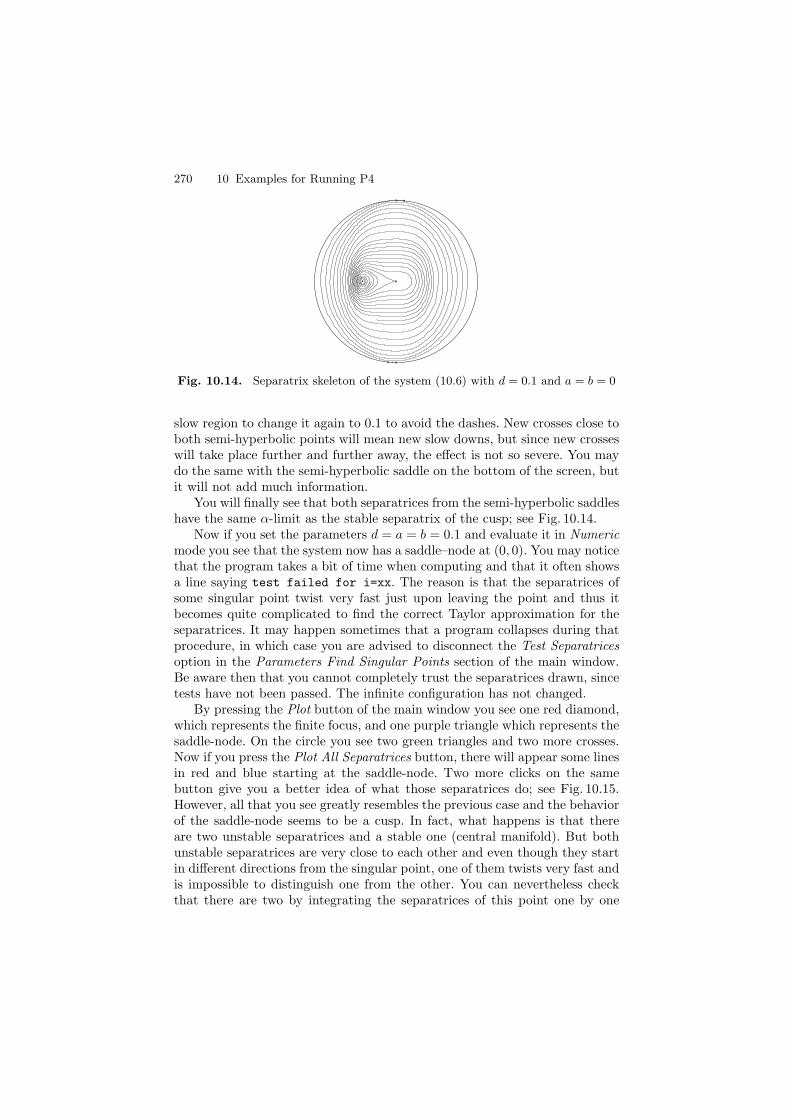
270 10 Examples for Running P4
Fig. 10.14. Separatrix skeleton of the system (10.6) with d = 0.1 and a = b = 0
slow region to change it again to 0.1 to avoid the dashes. New crosses close toboth semi-hyperbolic points will mean new slow downs, but since new crosseswill take place further and further away, the effect is not so severe. You maydo the same with the semi-hyperbolic saddle on the bottom of the screen, butit will not add much information.
You will finally see that both separatrices from the semi-hyperbolic saddleshave the same α-limit as the stable separatrix of the cusp; see Fig. 10.14.
Now if you set the parameters d = a = b = 0.1 and evaluate it in Numericmode you see that the system now has a saddle–node at (0, 0). You may noticethat the program takes a bit of time when computing and that it often showsa line saying test failed for i=xx. The reason is that the separatrices ofsome singular point twist very fast just upon leaving the point and thus itbecomes quite complicated to find the correct Taylor approximation for theseparatrices. It may happen sometimes that a program collapses during thatprocedure, in which case you are advised to disconnect the Test Separatricesoption in the Parameters Find Singular Points section of the main window.Be aware then that you cannot completely trust the separatrices drawn, sincetests have not been passed. The infinite configuration has not changed.
By pressing the Plot button of the main window you see one red diamond,which represents the finite focus, and one purple triangle which represents thesaddle-node. On the circle you see two green triangles and two more crosses.Now if you press the Plot All Separatrices button, there will appear some linesin red and blue starting at the saddle-node. Two more clicks on the samebutton give you a better idea of what those separatrices do; see Fig. 10.15.However, all that you see greatly resembles the previous case and the behaviorof the saddle-node seems to be a cusp. In fact, what happens is that thereare two unstable separatrices and a stable one (central manifold). But bothunstable separatrices are very close to each other and even though they startin different directions from the singular point, one of them twists very fast andis impossible to distinguish one from the other. You can nevertheless checkthat there are two by integrating the separatrices of this point one by one
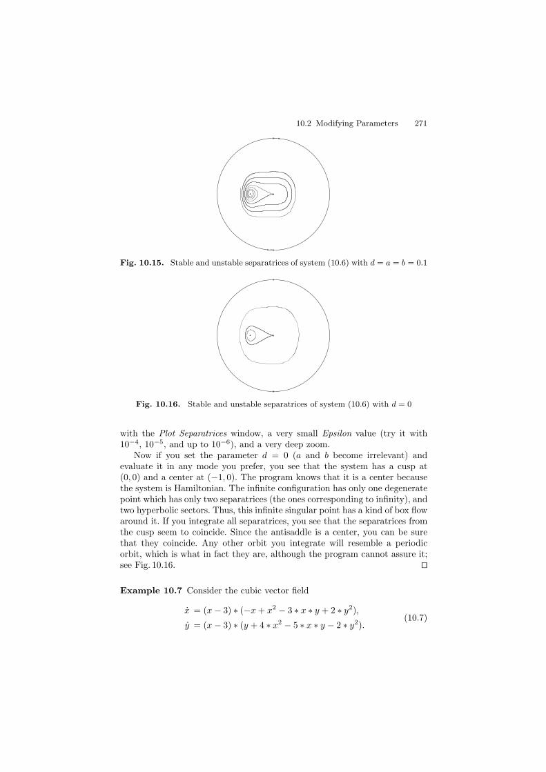
10.2 Modifying Parameters 271
Fig. 10.15. Stable and unstable separatrices of system (10.6) with d = a = b = 0.1
Fig. 10.16. Stable and unstable separatrices of system (10.6) with d = 0
with the Plot Separatrices window, a very small Epsilon value (try it with10−4, 10−5, and up to 10−6), and a very deep zoom.
Now if you set the parameter d = 0 (a and b become irrelevant) andevaluate it in any mode you prefer, you see that the system has a cusp at(0, 0) and a center at (−1, 0). The program knows that it is a center becausethe system is Hamiltonian. The infinite configuration has only one degeneratepoint which has only two separatrices (the ones corresponding to infinity), andtwo hyperbolic sectors. Thus, this infinite singular point has a kind of box flowaround it. If you integrate all separatrices, you see that the separatrices fromthe cusp seem to coincide. Since the antisaddle is a center, you can be surethat they coincide. Any other orbit you integrate will resemble a periodicorbit, which is what in fact they are, although the program cannot assure it;see Fig. 10.16. ⊓⊔
Example 10.7 Consider the cubic vector field
x = (x − 3) ∗ (−x + x2 − 3 ∗ x ∗ y + 2 ∗ y2),
y = (x − 3) ∗ (y + 4 ∗ x2 − 5 ∗ x ∗ y − 2 ∗ y2).(10.7)
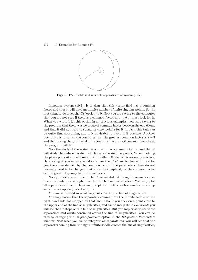
272 10 Examples for Running P4
Fig. 10.17. Stable and unstable separatrices of system (10.7)
Introduce system (10.7). It is clear that this vector field has a commonfactor and thus it will have an infinite number of finite singular points. So thefirst thing to do is set the Gcf option to 0. Now you are saying to the computerthat you are not sure if there is a common factor and that it must look for it.When you wrote 1 for this option in all previous examples, you were saying tothe program that there was no greatest common factor between the equations,and that it did not need to spend its time looking for it. In fact, this task canbe quite time-consuming and it is advisable to avoid it if possible. Anotherpossibility is to say to the computer that the greatest common factor is x− 3and that taking that, it may skip its computation also. Of course, if you cheat,the program will fail.
Now the study of the system says that it has a common factor, and that itwill study the reduced system which has some singular points. When plottingthe phase portrait you will see a button called GCF which is normally inactive.By clicking it you enter a window where the Evaluate button will draw foryou the curve defined by the common factor. The parameters there do notnormally need to be changed, but since the complexity of the common factorcan be great, they may help in some cases.
Now you see a green line in the Poincare disk. Although it seems a curveit corresponds to a straight line due to the compactification. You may plotall separatrices (one of them may be plotted better with a smaller time stepsince dashes appear); see Fig. 10.17.
You are interested in what happens close to the line of singularities.You may notice that the separatrix coming from the infinite saddle on the
right-hand side has stopped on that line. Also, if you click on a point close tothe upper end of the line of singularities, and ask to integrate it Backwards youwill see that it stops on the line of singularities. But you may wish to see thoseseparatices and orbits continued across the line of singularities. You can dothat by changing the Original/Reduced option in the Integration Parameterswindow. Now when you ask to integrate all separatrices, you will see that theseparatrix coming from the right infinite saddle crosses the line of singularities,
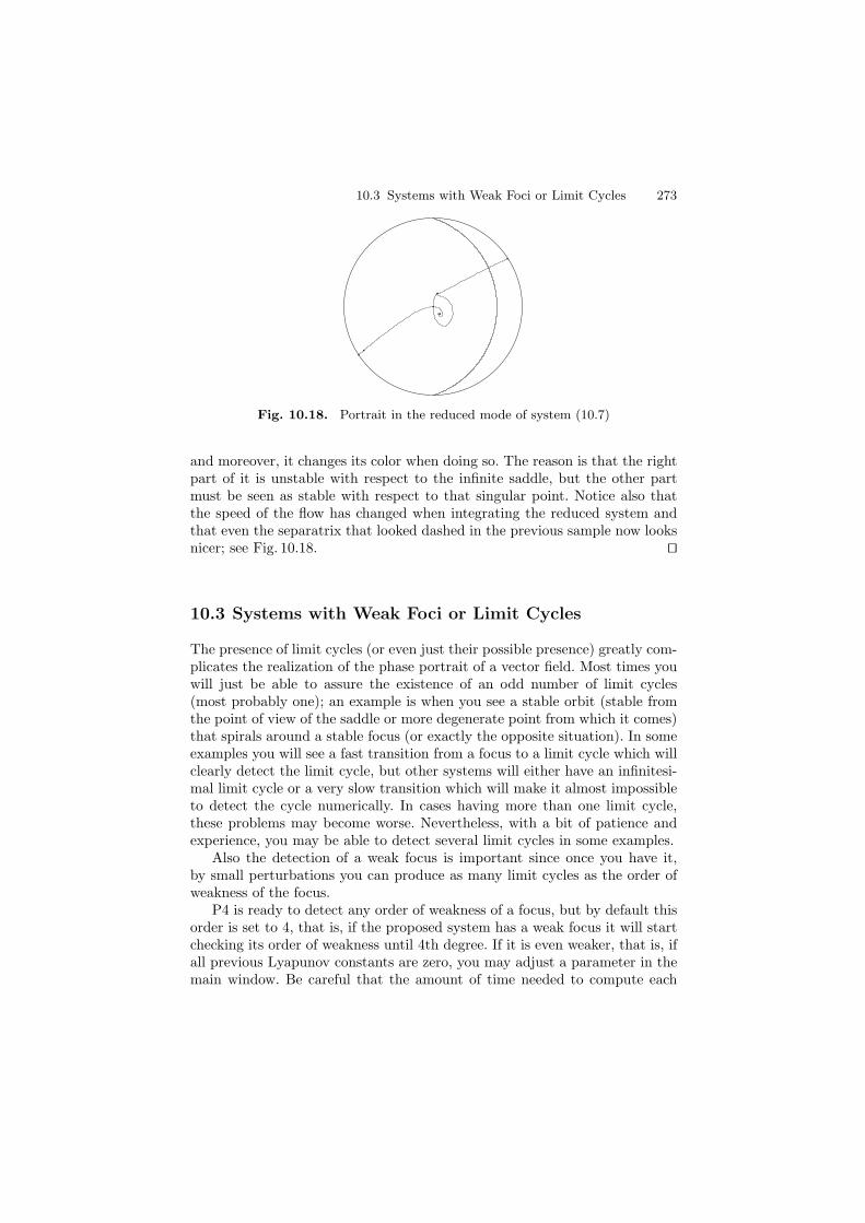
10.3 Systems with Weak Foci or Limit Cycles 273
Fig. 10.18. Portrait in the reduced mode of system (10.7)
and moreover, it changes its color when doing so. The reason is that the rightpart of it is unstable with respect to the infinite saddle, but the other partmust be seen as stable with respect to that singular point. Notice also thatthe speed of the flow has changed when integrating the reduced system andthat even the separatrix that looked dashed in the previous sample now looksnicer; see Fig. 10.18. ⊓⊔
10.3 Systems with Weak Foci or Limit Cycles
The presence of limit cycles (or even just their possible presence) greatly com-plicates the realization of the phase portrait of a vector field. Most times youwill just be able to assure the existence of an odd number of limit cycles(most probably one); an example is when you see a stable orbit (stable fromthe point of view of the saddle or more degenerate point from which it comes)that spirals around a stable focus (or exactly the opposite situation). In someexamples you will see a fast transition from a focus to a limit cycle which willclearly detect the limit cycle, but other systems will either have an infinitesi-mal limit cycle or a very slow transition which will make it almost impossibleto detect the cycle numerically. In cases having more than one limit cycle,these problems may become worse. Nevertheless, with a bit of patience andexperience, you may be able to detect several limit cycles in some examples.
Also the detection of a weak focus is important since once you have it,by small perturbations you can produce as many limit cycles as the order ofweakness of the focus.
P4 is ready to detect any order of weakness of a focus, but by default thisorder is set to 4, that is, if the proposed system has a weak focus it will startchecking its order of weakness until 4th degree. If it is even weaker, that is, ifall previous Lyapunov constants are zero, you may adjust a parameter in themain window. Be careful that the amount of time needed to compute each
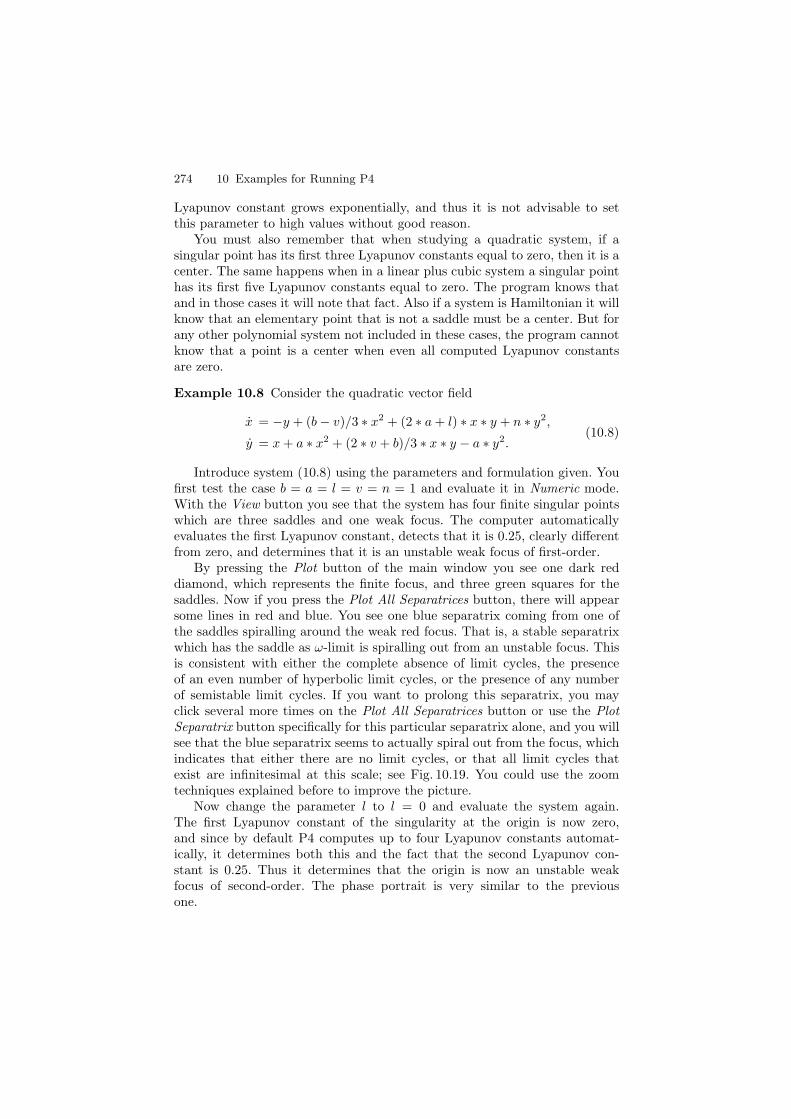
274 10 Examples for Running P4
Lyapunov constant grows exponentially, and thus it is not advisable to setthis parameter to high values without good reason.
You must also remember that when studying a quadratic system, if asingular point has its first three Lyapunov constants equal to zero, then it is acenter. The same happens when in a linear plus cubic system a singular pointhas its first five Lyapunov constants equal to zero. The program knows thatand in those cases it will note that fact. Also if a system is Hamiltonian it willknow that an elementary point that is not a saddle must be a center. But forany other polynomial system not included in these cases, the program cannotknow that a point is a center when even all computed Lyapunov constantsare zero.
Example 10.8 Consider the quadratic vector field
x = −y + (b − v)/3 ∗ x2 + (2 ∗ a + l) ∗ x ∗ y + n ∗ y2,
y = x + a ∗ x2 + (2 ∗ v + b)/3 ∗ x ∗ y − a ∗ y2.(10.8)
Introduce system (10.8) using the parameters and formulation given. Youfirst test the case b = a = l = v = n = 1 and evaluate it in Numeric mode.With the View button you see that the system has four finite singular pointswhich are three saddles and one weak focus. The computer automaticallyevaluates the first Lyapunov constant, detects that it is 0.25, clearly differentfrom zero, and determines that it is an unstable weak focus of first-order.
By pressing the Plot button of the main window you see one dark reddiamond, which represents the finite focus, and three green squares for thesaddles. Now if you press the Plot All Separatrices button, there will appearsome lines in red and blue. You see one blue separatrix coming from one ofthe saddles spiralling around the weak red focus. That is, a stable separatrixwhich has the saddle as ω-limit is spiralling out from an unstable focus. Thisis consistent with either the complete absence of limit cycles, the presenceof an even number of hyperbolic limit cycles, or the presence of any numberof semistable limit cycles. If you want to prolong this separatrix, you mayclick several more times on the Plot All Separatrices button or use the PlotSeparatrix button specifically for this particular separatrix alone, and you willsee that the blue separatrix seems to actually spiral out from the focus, whichindicates that either there are no limit cycles, or that all limit cycles thatexist are infinitesimal at this scale; see Fig. 10.19. You could use the zoomtechniques explained before to improve the picture.
Now change the parameter l to l = 0 and evaluate the system again.The first Lyapunov constant of the singularity at the origin is now zero,and since by default P4 computes up to four Lyapunov constants automat-ically, it determines both this and the fact that the second Lyapunov con-stant is 0.25. Thus it determines that the origin is now an unstable weakfocus of second-order. The phase portrait is very similar to the previousone.
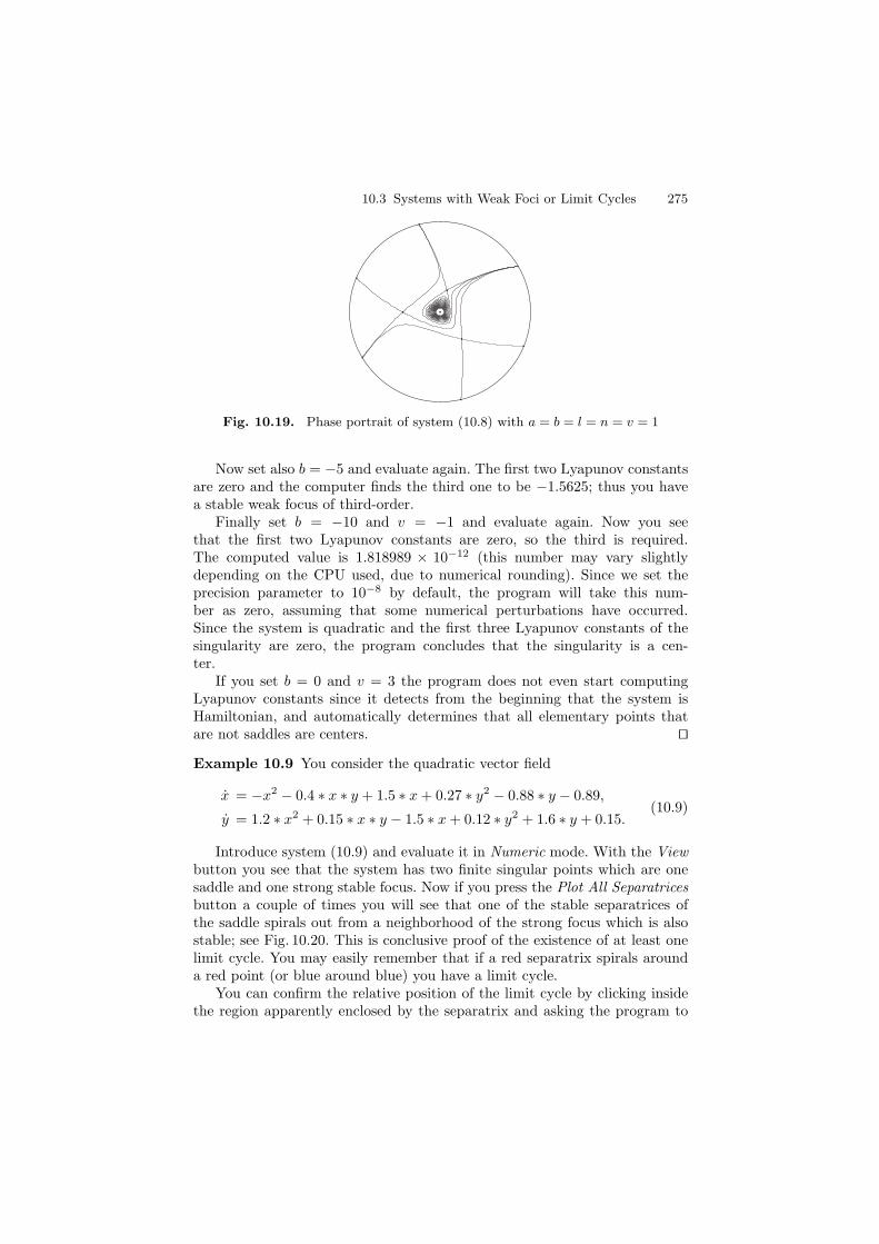
10.3 Systems with Weak Foci or Limit Cycles 275
Fig. 10.19. Phase portrait of system (10.8) with a = b = l = n = v = 1
Now set also b = −5 and evaluate again. The first two Lyapunov constantsare zero and the computer finds the third one to be −1.5625; thus you havea stable weak focus of third-order.
Finally set b = −10 and v = −1 and evaluate again. Now you seethat the first two Lyapunov constants are zero, so the third is required.The computed value is 1.818989 × 10⁻¹² (this number may vary slightlydepending on the CPU used, due to numerical rounding). Since we set theprecision parameter to 10−8 by default, the program will take this num-ber as zero, assuming that some numerical perturbations have occurred.Since the system is quadratic and the first three Lyapunov constants of thesingularity are zero, the program concludes that the singularity is a cen-ter.
If you set b = 0 and v = 3 the program does not even start computingLyapunov constants since it detects from the beginning that the system isHamiltonian, and automatically determines that all elementary points thatare not saddles are centers. ⊓⊔
Example 10.9 You consider the quadratic vector field
x = −x2 − 0.4 ∗ x ∗ y + 1.5 ∗ x + 0.27 ∗ y2 − 0.88 ∗ y − 0.89,
y = 1.2 ∗ x2 + 0.15 ∗ x ∗ y − 1.5 ∗ x + 0.12 ∗ y2 + 1.6 ∗ y + 0.15.(10.9)
Introduce system (10.9) and evaluate it in Numeric mode. With the Viewbutton you see that the system has two finite singular points which are onesaddle and one strong stable focus. Now if you press the Plot All Separatricesbutton a couple of times you will see that one of the stable separatrices ofthe saddle spirals out from a neighborhood of the strong focus which is alsostable; see Fig. 10.20. This is conclusive proof of the existence of at least onelimit cycle. You may easily remember that if a red separatrix spirals arounda red point (or blue around blue) you have a limit cycle.
You can confirm the relative position of the limit cycle by clicking insidethe region apparently enclosed by the separatrix and asking the program to
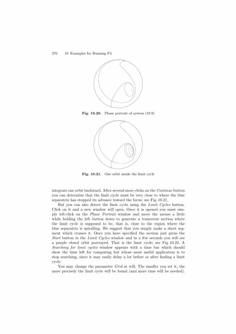
276 10 Examples for Running P4
Fig. 10.20. Phase portrait of system (10.9)
Fig. 10.21. One orbit inside the limit cycle
integrate one orbit backward. After several more clicks on the Continue buttonyou can determine that the limit cycle must be very close to where the blueseparatrix has stopped its advance toward the focus; see Fig. 10.21.
But you can also detect the limit cycle using the Limit Cycles button.Click on it and a new window will open. Once it is opened you must sim-ply left-click on the Phase Portrait window and move the mouse a littlewhile holding the left button down to generate a transverse section wherethe limit cycle is supposed to be, that is, close to the region where theblue separatrix is spiralling. We suggest that you simply make a short seg-ment which crosses it. Once you have specified the section just press theStart button in the Limit Cycles window and in a few seconds you will seea purple closed orbit portrayed. That is the limit cycle; see Fig. 10.22. ASearching for limit cycles window appears with a time bar which shouldshow the time left for computing but whose most useful application is tostop searching, since it may easily delay a lot before or after finding a limitcycle.
You may change the parameter Grid at will. The smaller you set it, themore precisely the limit cycle will be found (and more time will be needed).
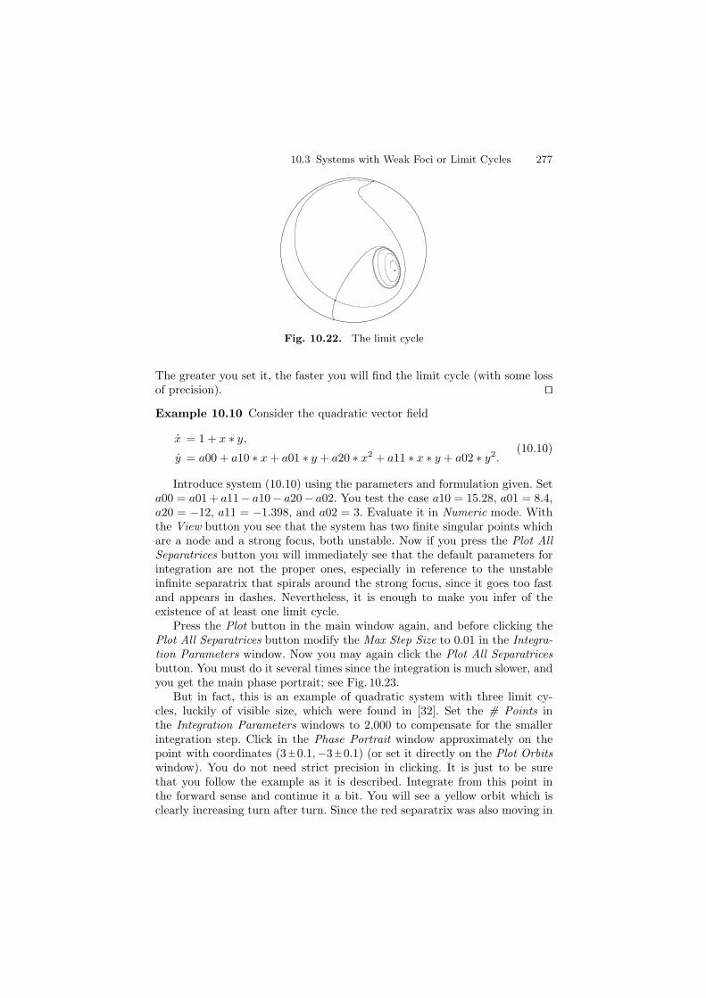
10.3 Systems with Weak Foci or Limit Cycles 277
Fig. 10.22. The limit cycle
The greater you set it, the faster you will find the limit cycle (with some lossof precision). ⊓⊔
Example 10.10 Consider the quadratic vector field
x = 1 + x ∗ y,
y = a00 + a10 ∗ x + a01 ∗ y + a20 ∗ x2 + a11 ∗ x ∗ y + a02 ∗ y2.(10.10)
Introduce system (10.10) using the parameters and formulation given. Seta00 = a01 + a11− a10− a20− a02. You test the case a10 = 15.28, a01 = 8.4,a20 = −12, a11 = −1.398, and a02 = 3. Evaluate it in Numeric mode. Withthe View button you see that the system has two finite singular points whichare a node and a strong focus, both unstable. Now if you press the Plot AllSeparatrices button you will immediately see that the default parameters forintegration are not the proper ones, especially in reference to the unstableinfinite separatrix that spirals around the strong focus, since it goes too fastand appears in dashes. Nevertheless, it is enough to make you infer of theexistence of at least one limit cycle.
Press the Plot button in the main window again, and before clicking thePlot All Separatrices button modify the Max Step Size to 0.01 in the Integra-tion Parameters window. Now you may again click the Plot All Separatricesbutton. You must do it several times since the integration is much slower, andyou get the main phase portrait; see Fig. 10.23.
But in fact, this is an example of quadratic system with three limit cy-cles, luckily of visible size, which were found in [32]. Set the # Points inthe Integration Parameters windows to 2,000 to compensate for the smallerintegration step. Click in the Phase Portrait window approximately on thepoint with coordinates (3 0.1,−3 0.1) (or set it directly on the Plot Orbitswindow). You do not need strict precision in clicking. It is just to be surethat you follow the example as it is described. Integrate from this point inthe forward sense and continue it a bit. You will see a yellow orbit which isclearly increasing turn after turn. Since the red separatrix was also moving in
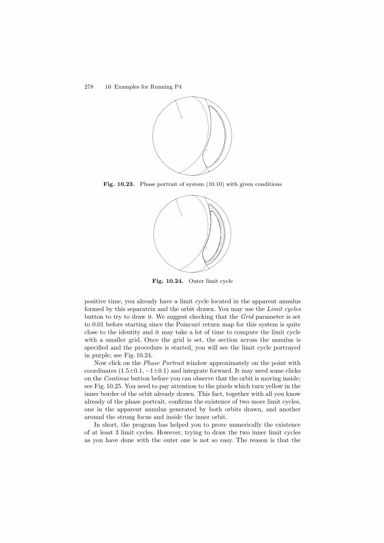
278 10 Examples for Running P4
Fig. 10.23. Phase portrait of system (10.10) with given conditions
Fig. 10.24. Outer limit cycle
positive time, you already have a limit cycle located in the apparent annulusformed by this separatrix and the orbit drawn. You may use the Limit cyclesbutton to try to draw it. We suggest checking that the Grid parameter is setto 0.01 before starting since the Poincare return map for this system is quiteclose to the identity and it may take a lot of time to compute the limit cyclewith a smaller grid. Once the grid is set, the section across the annulus isspecified and the procedure is started, you will see the limit cycle portrayedin purple; see Fig. 10.24.
Now click on the Phase Portrait window approximately on the point withcoordinates (1.5 0.1,−1 0.1) and integrate forward. It may need some clickson the Continue button before you can observe that the orbit is moving inside;see Fig. 10.25. You need to pay attention to the pixels which turn yellow in theinner border of the orbit already drawn. This fact, together with all you knowalready of the phase portrait, confirms the existence of two more limit cycles,one in the apparent annulus generated by both orbits drawn, and anotheraround the strong focus and inside the inner orbit.
In short, the program has helped you to prove numerically the existenceof at least 3 limit cycles. However, trying to draw the two inner limit cyclesas you have done with the outer one is not so easy. The reason is that the
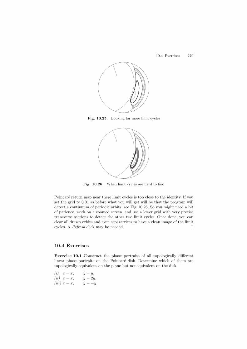
10.4 Exercises 279
Fig. 10.25. Looking for more limit cycles
Fig. 10.26. When limit cycles are hard to find
Poincare return map near these limit cycles is too close to the identity. If youset the grid to 0.01 as before what you will get will be that the program willdetect a continuum of periodic orbits; see Fig. 10.26. So you might need a bitof patience, work on a zoomed screen, and use a lower grid with very precisetransverse sections to detect the other two limit cycles. Once done, you canclear all drawn orbits and even separatrices to have a clean image of the limitcycles. A Refresh click may be needed. ⊓⊔
10.4 Exercises
Exercise 10.1 Construct the phase portraits of all topologically differentlinear phase portraits on the Poincare disk. Determine which of them aretopologically equivalent on the plane but nonequivalent on the disk.
(i) x = x, y = y,(ii) x = x, y = 2y,(iii) x = x, y = −y,

280 10 Examples for Running P4
(iv) x = x + y, y = −3x + 2y,(v) x = −y, y = x,(vi) x = y, y = 1,(vii) x = x, y = 1,(viii)x = x, y = 0,(ix) x = y, y = 0.(x) x = x + y, y = y.
Exercise 10.2 Prove that the following system forms a rotated vector fieldfamily with rotation parameter α, and has a semistable limit cycle x2 +y2−1of multiplicity two for α = 0, using the tools given in Chap. 7.
x = − y + x(x2 + y2 − 1)2,
y =x + y(x2 + y2 − 1)2 + α(−y + x(x2 + y2 − 1)2).
Also prove for which sign of α (either positive or negative) you have twohyperbolic limit cycles, and check it numerically with P4.
Exercise 10.3 Construct the phase portrait of system
x = y + x2 − x2y + 2y3,
y = x + y2 − x3 − xy2,
check that there is a finite limit cycle, and show that the circle at infinity (theequator of the Poincare sphere) behaves like a semistable limit cycle. Now youperturb the infinite limit cycle by adding some higher order terms, trying toproduce a finite limit cycle. Determine a value of ε for which there are twofinite limit cycles for
x = y + x2 − x2y + 2y3 + ε(x3y + y4),
y =x + y2 − x3 − xy2 + εx2y2.
Then use a rotated vector field family
x = y + x2 − x2y + 2y3 + ε(x3y + y4),
y = x + y2 − x3 − xy2 + εx2y2 + α(y + x2 − x2y + 2y3 + ε(x3y + y4)),
so as to reduce the distance that separates the limit cycles, and get an approx-imation of the value of the rotation parameter for which a finite semistablelimit cycle occurs. You will see that it is impossible to be certain of the valuefor which the semistable limit cycle exists. At most, you can be sure thatfor a certain value of α there are two limit cycle, and for another, there isnone.
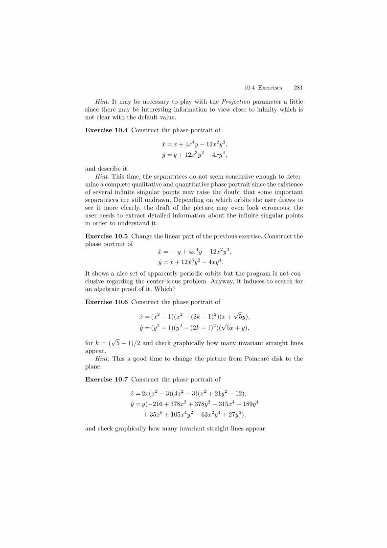
10.4 Exercises 281
Hint: It may be necessary to play with the Projection parameter a littlesince there may be interesting information to view close to infinity which isnot clear with the default value.
Exercise 10.4 Construct the phase portrait of
x = x + 4x4y − 12x2y3,
y = y + 12x3y2 − 4xy4,
and describe it.Hint: This time, the separatrices do not seem conclusive enough to deter-
mine a complete qualitative and quantitative phase portrait since the existenceof several infinite singular points may raise the doubt that some importantseparatrices are still undrawn. Depending on which orbits the user draws tosee it more clearly, the draft of the picture may even look erroneous; theuser needs to extract detailed information about the infinite singular pointsin order to understand it.
Exercise 10.5 Change the linear part of the previous exercise. Construct thephase portrait of
x = − y + 4x4y − 12x2y3,
y =x + 12x3y2 − 4xy4.
It shows a nice set of apparently periodic orbits but the program is not con-clusive regarding the center-focus problem. Anyway, it induces to search foran algebraic proof of it. Which?
Exercise 10.6 Construct the phase portrait of
x = (x2 − 1)(x2 − (2k − 1)2)(x +√
5y),
y = (y2 − 1)(y2 − (2k − 1)2)(√
5x + y),
for k = (√
5 − 1)/2 and check graphically how many invariant straight linesappear.
Hint: This a good time to change the picture from Poincare disk to theplane.
Exercise 10.7 Construct the phase portrait of
x = 2x(x2 − 3)(4x2 − 3)(x2 + 21y2 − 12),
y = y(−216 + 378x2 + 378y2 − 315x4 − 189y4
+ 35x6 + 105x4y2 − 63x2y4 + 27y6),
and check graphically how many invariant straight lines appear.
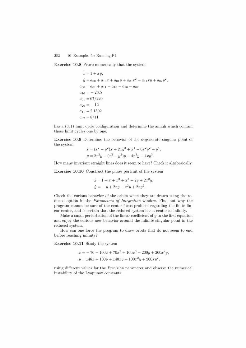
282 10 Examples for Running P4
Exercise 10.8 Prove numerically that the system
x = 1 + xy,
y = a00 + a10x + a01y + a20x2 + a11xy + a02y
2,
a00 = a01 + a11 − a10 − a20 − a02
a10 = − 26.5
a01 = 67/220
a20 = − 12
a11 = 2.1502
a02 = 8/11
has a (3, 1) limit cycle configuration and determine the annuli which containthose limit cycles one by one.
Exercise 10.9 Determine the behavior of the degenerate singular point ofthe system
x = (x2 − y2)x + 2xy2 + x4 − 6x2y2 + y4,
y = 2x2y − (x2 − y2)y − 4x3y + 4xy3.
How many invariant straight lines does it seem to have? Check it algebraically.
Exercise 10.10 Construct the phase portrait of the system
x = 1 + x + x2 + x3 + 2y + 2x2y,
y = − y + 2xy + x2y + 2xy2.
Check the curious behavior of the orbits when they are drawn using the re-duced option in the Parameters of Integration window. Find out why theprogram cannot be sure of the center-focus problem regarding the finite lin-ear center, and is certain that the reduced system has a center at infinity.
Make a small perturbation of the linear coefficient of y in the first equationand enjoy the curious new behavior around the infinite singular point in thereduced system.
How can one force the program to draw orbits that do not seem to endbefore reaching infinity?
Exercise 10.11 Study the system
x = − 70 − 100x + 70x2 + 100x3 − 200y + 200x2y,
y = 146x + 100y + 140xy + 100x2y + 200xy2,
using different values for the Precision parameter and observe the numericalinstability of the Lyapunov constants.
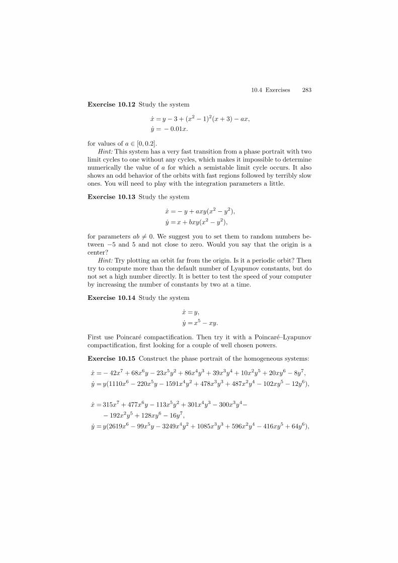
10.4 Exercises 283
Exercise 10.12 Study the system
x = y − 3 + (x2 − 1)2(x + 3) − ax,
y = − 0.01x.
for values of a ∈ [0, 0.2].Hint: This system has a very fast transition from a phase portrait with two
limit cycles to one without any cycles, which makes it impossible to determinenumerically the value of a for which a semistable limit cycle occurs. It alsoshows an odd behavior of the orbits with fast regions followed by terribly slowones. You will need to play with the integration parameters a little.
Exercise 10.13 Study the system
x = − y + axy(x2 − y2),
y =x + bxy(x2 − y2),
for parameters ab �= 0. We suggest you to set them to random numbers be-tween −5 and 5 and not close to zero. Would you say that the origin is acenter?
Hint: Try plotting an orbit far from the origin. Is it a periodic orbit? Thentry to compute more than the default number of Lyapunov constants, but donot set a high number directly. It is better to test the speed of your computerby increasing the number of constants by two at a time.
Exercise 10.14 Study the system
x = y,
y = x5 − xy.
First use Poincare compactification. Then try it with a Poincare–Lyapunovcompactification, first looking for a couple of well chosen powers.
Exercise 10.15 Construct the phase portrait of the homogeneous systems:
x = − 42x7 + 68x6y − 23x5y2 + 86x4y3 + 39x3y4 + 10x2y5 + 20xy6 − 8y7,
y = y(1110x6 − 220x5y − 1591x4y2 + 478x3y3 + 487x2y4 − 102xy5 − 12y6),
x = 315x7 + 477x6y − 113x5y2 + 301x4y3 − 300x3y4−− 192x2y5 + 128xy6 − 16y7,
y = y(2619x6 − 99x5y − 3249x4y2 + 1085x3y3 + 596x2y4 − 416xy5 + 64y6),

284 10 Examples for Running P4
A B C
Fig. 10.27. Exercise 10.16
x = 6x7 + 4x6y − 15x5y2 − 10x4y3 − 33x3y4 − 22x2y5 − 12xy6 − 8y7,
y = y(−90x6 − 28x5y + 201x4y2 + 62x3y3 − 177x2y4 − 70xy5 + 12y6),
x = − 45x7 − 9x6y + 155x5y2 + 31x4y3 + 120x3y4+
+ 24x2y5 − 80xy6 − 16y7,
y = y(2619x6 − 99x5y − 3249x4y2 + 1085x3y3 + 596x2y4 − 416xy5 + 64y6),
x = y2(25x5 + 20x4y + 18x3y2 + 18x2y3 − 7xy4 − 2y5),
y = y(288x6 − 72x5y − 367x4y2 + 118x3y3 + 130x2y4 − 10xy5 − 15y6).
Exercise 10.16 Consider the system
x′ = y + 4x(x + y), y′ = x2 + 4xy + 3y2. (10.11)
The finite singularities of system (10.11) are P0(0, 0) which is a second-ordercusp and P1(1/8,−1/24), an unstable hyperbolic node. At infinity there isa stable node at (1, 0) of local chart U1, a saddle at the origin of U2 and asaddle–node coming from the collision of a finite singularity with an infiniteone located at (−1, 0) of U1. The phase portrait of system (10.11) is given inFig. 10.27a.
Make some linear and constant small perturbations to system (10.11) suchthat you split the cusp into an elementary saddle and an elementary stable orunstable node, in a way that yields the phase portraits given in Fig. 10.27b, c.
Hint: The perturbations may be very small and thus the quantitative imagethat you get with P4 at normal zoom appear different, or simply difficult tograsp.
Bibliography
1. M.I. Al’mukhamedov. On the construction of a differential equation havinggiven curves as limit cycles. Izv. Vyss. Ucebn. Zaved Matematika (in Russian),44:3–6, 1963.
2. A.F. Andreev. Investigation of the behaviour of the integral curves of a systemof two differential equations in the neighbourhood of a singular point. Trans.Amer. Math. Soc. 8:183–207, 1958.
3. A.A. Andronov. Les cycles limites de Poincare et la theorie des oscillationsauto–entretenues. C.R. Acad. Sci. Paris, 189:559–561, 1929.
4. A.A. Andronov, E.A. Leontovich, I.I. Gordon, and A.G. Maier. Qualitativetheory of second–order dynamic systems. Israel Program for Scientific Trans-lations. Halsted Press (A division of Wiley), New York, 1973.
5. V.I. Arnol’d. Geometrical methods in the theory of ordinary differential equa-tions. Fundamental Principles of Mathematical Science. Springer, Berlin Hei-delberg New York, 1983.
6. V.I. Arnol’d and Y. Il’Yashenko. Ordinary differential equations, pages 1–148.Encyclopaedia Math. Sci., 1, Dynamical systems, I. Springer, Berlin HeidelbergNew York, 1988.
7. V.I. Arnol’d, A. Varchenko, and S. Goussien-Zade. Singularites des applicationsdifferentiables. Israel Program for Scientific Translations. Mir, Moscow, 1982.
8. D.K. Arrowsmith. The singularity x ∂/∂y. J. Differ. Equat., 34:153–166, 1979.9. J.C. Artes, F. Dumortier, C. Herssens, J. Llibre, and P. De Maesschalck. Com-
puter program P4 to study Phase Portraits of Planar Polynomial differentialequations. http://mat.uab.es/∼artes/p4/p4.htm, 2005.
10. J.C. Artes, R. Kooij, and J. Llibre. Sructurally stable quadratic vector fields.Mem. Am. Math. Soc. 134(639), 1998.
11. J.C. Artes, J. Llibre, and J. C. Medrano. Nonexistence of limit cycles for aclass of structurally stable quadratic vector fields. Preprint, 2005.
12. F. Balibrea and V. Jimenez. A characterization of the ω-limit sets of planarcontinuous dynamical systems. J. Differ. Equat. 145:469–488, 1998.
13. R. Bamon. Quadratic vector fields in the plane have a finite number of limitcycles. Int. Hautes Etudes Sci. Publ. Math. 64:111–142, 1986.
14. N.N. Bautin. On the number of limit cycles which appear with the variationof the coefficients from an equilibrium position of focus or center type. Math.USSR–Sb. 100:397–413, 1954.
286 Bibliography
15. I. Bendixson. Sur les courbes definies par des equations differentielles. ActaMath. 24:1–88, 1901.
16. A.N. Berlinskii. On the number of elliptic domains adherent to a singularity.Soviet Math. Dokl. 9:169–173, 1968.
17. A.N. Berlinskii. On the structure of the neighborhood of a singular point of atwo-dimensional autonomous system. Soviet Math. Dokl. 10:882–885, 1969.
18. E. Bierstone and P.D. Milman. Semi-analytic and subanalytic sets. Inst. Hautestudes Sci. Publ. Math. 67:5–42, 1988.
19. Th. Brocker. Differentiable germs and catastrophes. London Math. Soc. Lect.Note Ser. 17, 1975.
20. H. Broer. Formal normal forms theorems for vector fields and some conse-quences for bifurcations in the volume preserving case. Springer Lecture Notesin Maths. 898:54–74, 1981.
21. I.U. Bronstein and A.Y. Kopanskii. Smooth invariant manifolds and normalforms. World Scientific Series on Nonlinear Science, volume 7 of Series A:Monographs and Treatises. World Scientific, Singapore, 1994.
22. M. Brunella and M. Miari. Topological equivalence of a plane vector fieldwith its principal part defined through Newton polyhedra. J. Differ. Equat.85:338–366, 1990.
23. A.D. Bruno. Local methods in non–linear differential equations. Springer SeriesSoviet Math. Springer, Berlin Heidelberg New York, 1989.
24. L. Cairo, M.R. Feix, and J. Llibre. Integrability and algebraic solutions forplanar polynomial differential systems with emphasis on the quadratic systems.Resenhas, 4:127–161, 1999.
25. L. Cairo and J. Llibre. Darbouxian first integrals and invariants for realquadratic systems having an invariant conic. J. Phys. A: Math. Gen. 35:589–608, 2002.
26. J. Carr. Applications of centre manifold theory. Applied Mathematical Sci-ences. Springer, Berlin Heidelberg New York, 1981.
27. M. Caubergh and F. Dumortier. Hopf–Takens bifurcations and centres. J.Differ. Equat., 202:1–31, 2004.
28. J. Chavarriga and J. Gine. Integrability of a linear center perturbed by fourthdegree homogeneous polynomial. Publicacions Matematiques, 40:21–39, 1996.
29. J. Chavarriga and J. Gine. Integrability of a linear center perturbed by fifth de-gree homogeneous polynomial. Publicacions Matematiques, 41:335–356, 1997.
30. J. Chavarriga and J. Gine. Integrability of cubic with degenerate infinity.Differ. Equat. Dyn. Syst. 6:425–438, 1998.
31. J. Chavarriga, J. Llibre, and J. Sotomayor. Invariant algebraic solutions forpolynomial systems with emphasis in the quadratic case. Expositiones Math.15:161–173, 1997.
32. L.A. Cherkas, J.C. Artes, and J. Llibre. Quadratic systems with limit cyclesof normal size. Bull. Acad. Stiinte Repub. Mold. Mat., 1:31–46, 2003.
33. C. Chicone and F. Dumortier. Finiteness for critical points of planar analyticvector fields. Nonlinear Anal. Theor. Methods Appl. pages 315–335, 1993.
34. C. Chicone and W. Liu. Asymptotic phase revisited. J. Differ. Equat. 204:227–246, 2004.
35. S.N. Chow and J.K. Hale. Methods of bifurcation theory, volume 251 ofGrundlehren der Mathematischen Wissenschaften [Fundamental Principles ofMathematical Science]. Springer, Berlin Heidelberg New York, 1982.
Bibliography 287
36. S.N. Chow, C.Z. Li, and D. Wang. Normal forms and bifurcation of planarvector fields. Grundlehren der Mathematischen Wissenschaften [FundamentalPrinciples of Mathematical Science]. Cambridge University Press, Cambridge,1994.
37. C.J. Christopher. Invariant algebraic curves and conditions for a center. Proc.Roy. Soc. Edinburgh, 124A:1209–1229, 1994.
38. C.J. Christopher and J. Llibre. Algebraic aspects of integrability for polynomialsystems. Qualit. Theor. Dyn. Syst. 1:71–95, 1999.
39. C.J. Christopher and J. Llibre. Integrability via invariant algebraic curves forplanar polynomial differential systems. Ann. Differ. Equat. 16:5–19, 2000.
40. C.J. Christopher, J. Llibre, and J.V. Pereira. Multiplicity of invariant algebraiccurves in polynomial vector fields. Preprint, 2004.
41. A. Cima, A. Gasull, V. Manosa, and F. Manosas. Algebraic properties of theLyapunov and period constants. Rocky Mountain J. Math. 27:471–501, 1997.
42. A. Cima, A. Gasull, and J. Torregrosa. On the relation between index andmultplicity. J. London Math. Soc. 57:757–768, 1998.
43. J.L. Coolidge. A Treatise on algebraic plane curves. Dover, New York, 1959.44. W.A. Coppel. Stability and asymptotic behavior of differential equations.
Heath, Boston, 1965.45. W.A. Coppel. A survey of quadratic systems. J. Differ. Equat. 2:293–304,
1966.46. G. Darboux. Memoire sur les equations differentielles algebriques du premier
ordre et du premier degre (melanges). Bull. Sci. Math. 124A:60–96, 123–144,151–200, 1878.
47. J. Devlin. Word problems related to periodic solutions of a non–autonomoussystem. Math. Proc. Cambridge Philos. Soc. 108:127–151, 1990.
48. J. Devlin. Word problems related to derivatives of the displacement map.Math. Proc. Cambridge Philos. Soc. 110:569–579, 1991.
49. G.T. dos Santos. Classification of generic quadratic vector fields without limitcycles, volume 597 of Lect. Notes in Math, pages 605–640. Springer, BerlinHeidelberg New York, 1977.
50. G.F.D. Duff. Limit cycles and rotated vector fields. Ann. Math. 57:15–31,1953.
51. H. Dulac. Sur les cycles limites. Bull. Soc. Math. Fr. 51:45–188, 1953.52. F. Dumortier. Singularities of vector fields on the plane. J. Differ. Equat.
23:53–106, 1977.53. F. Dumortier. Singularities of vector fields, volume 32 of Monografias de
Matematica. IMPA, Rio de Janeiro, 1978.54. F. Dumortier and P. Fiddelaers. Quadratic models for generic local 3–
parameter bifurcations on the plane. Trans. Am. Math. Soc. 326:101–126,1991.
55. F. Dumortier and C. Herssens. Polynomial Lienard equations near infinity. J.Differ. Equat. 153:1–29, 1999.
56. F. Dumortier and C. Li. Quadratic Lienard equations with quadratic damping.J. Differ. Equat., 139:41–59, 1997.
57. F. Dumortier, P. Rodrigues, and R. Roussarie. Germs of diffeomorphismson the plane, volume 902 of Lectures Notes in Mathematics. Springer, BerlinHeidelberg New York, 1981.
58. F. Dumortier and C. Rousseau. Cubic Lienard equations with linear damping.Nonlinearity, 3:1015–1039, 1990.
288 Bibliography
59. J. Ecalle. Introduction aux fonctions analysables et preuve constructive de laconjecture de Dulac. Actualites Math. Hermann, Paris, 1992.
60. D. Eisenbud and H. Levine. An algebraic formula for the degree of a C∞ mapgerm. Ann. Math. 106:19–44, 1977.
61. C. Elphick, E. Tirapegui, M.E. Brachet, P. Coullet, and G. Iooss. A simpleglobal characterization for normal forms of singular vector fields. Phys. D,29:95–127, 1987.
62. W.W. Farr, Chengzhi Li, I.S. Labouriau, and W.F. Langford. Degenerate Hopfbifurcation formulas and Hilbert’s 16th problem. SIAM J. Math. Anal. 20:13–29, 1989.
63. E. Fehlberg. Classical fifth–, sixth–, seventh–, and eight–order Runge–Kuttaformulas with step size control, volume 287. NASA Technical Report, 1968.
64. N. Fenichel. Persistence and smoothness of invariant manifolds for flows. In-diana Univ. Math. J. 21:193–226, 1971.
65. J.P. Francoise. Successive derivatives of a first return map, application to thestudy of quadratic vector fields. Ergodic Theory Dyn. Syst. 16:87–96, 1996.
66. J.P. Francoise and R. Pons. Computer algebra methods and the stability ofdifferential systems. Random Comput. Dyn. 3:265–287, 1995.
67. J.P. Francoise and Y. Yomdin. Bernstein inequalities and applications to ana-lytic geometry and differential equations. J. Funct. Anal. 146:185–205, 1997.
68. E. Freire, A. Gasull, and A. Guillamon. Limit cycles and lie symmetries.Preprint, 2004.
69. A. Gasull, A. Guillamon, and V. Manosa. An explicit expression of thefirst Lyapunov and period constants with applications. J. Math. Anal. Appl.211:190–202, 1997.
70. A. Gasull, A. Guillamon, and V. Manosa. An analytic–numerical methodof computation of the Lyapunov and period constants from their algebraicstructure. SIAM J. Numer. Anal. 36:1030–1043, 1999.
71. A. Gasull and J. Torregrosa. A new approach to the computation of theLyapunov constants. Comput. Appl. Math. 20:149–177, 2001.
72. H. Giacomini, J. Llibre, and M. Viano. On the nonexistence, existence anduniqueness of limit cycles. Nonlinearity, 9:501–516, 1996.
73. M.G. Golitsina. Nonproper polycycles of quadratic vector fields on the plane.Selected translations, Selecta Math. Soviet., 10:143–155, 1991. translation ofMethods of the qualitative theory of differential equations (Russian), 51–67,Gor’kov. Gos. University, Gorki, 1987.
74. M. Golubitsky and D.G. Schaeffer. Singularities and groups in bifurcationtheory. Vol. I, volume 51 of Applied Mathematical Sciences. Springer, BerlinHeidelberg New York, 1985.
75. M. Golubitsky and D.G. Schaeffer. Singularities and groups in bifurcationtheory. Vol. II, volume 69 of Applied Mathematical Sciences. Springer, BerlinHeidelberg New York, 1988.
76. E.A.V. Gonzales. Generic properties of polynomial vector fields at infinity.Trans. Amer. Math. Soc. 143:201–222, 1969.
77. J. Guckenheimer and P. Holmes. Nonlinear oscillations, dynamical systems,and bifurcations of vector fields, volume 42 of Applied Mathematical Sciences.Springer, Berlin Heidelberg New York, 1983.
78. A. Guillamon. Estudi d’alguns problemes de teoria qualitativa al pla, ambaplicacions als sistemes depredador–presa. PhD thesis, Universitat Autonomade Barcelona, July 1995.

Bibliography 289
79. C. Gutierrez and J. Llibre. Darboux integrability for polynomial vector fieldson the 2 dimensional sphere. Extracta Math. 17:289–301, 2002.
80. P. Hartman. Ordinary differential equations. Wiley New York London Sydney,1964.
81. A.C. Hearn and J.P. Fitch. Reduce 3.6, user’s manual. Konrad–Zuse–Zentrum,Berlin, 1995.
82. D. Hilbert. Mathematische probleme. In Nachr. Ges. Wiss., editor, SecondInternat. Congress Math. Paris, 1900, pages 253–297. Gottingen Math.–Phys.Kl., 1900.
83. M. Hirsch, C.C. Pugh, and M. Shub. Invariant manifolds, volume 583 of Lec-tures Notes in Mathematics. Springer, Berlin Heidelberg New York, 1977.
84. W. Hirsch and S. Smale. Differential equations, dynamical systems, and linearalgebra, volume 60 of Pure and Applied Mathematics. Academic Press, NewYork London, 1974.
85. H. Hopf. Differential geometry in the large, volume 1000 of Lecture Notes inMath. Springer, Berlin Heidelberg New York, 1989.
86. I.D. Iliev. On second order bifurcations of limit cycles. J. London Math. Soc.58:353–366, 1998.
87. I.D. Iliev and L.M. Perko. Higher order bifurcations of limit cycles. J. Differ.Equat. 154:339–363, 1999.
88. Y. Il’Yashenko. Finiteness theorem for limit cycles, volume 94 of Trans. ofMath. Monogr. Am. Math. Soc. 1991.
89. Y. Il’Yashenko. Centennial history of Hilbert’s 16th problem. Bull. Am. Math.Soc. 39:301–354, 2002.
90. Y. Il’Yashenko and S. Yakovenko. Lectures on analytic differential equations.to be published.
91. Y. Il’Yashenko and S. Yakovenko. Finitely smooth normal forms of local fam-ilies of diffeomorphisms and vector fields. Uspekhi Mat. Nauk, 46:3–39, 1991.translation in Russian Math. Surveys 46 (1991), no. 1, 1–43.
92. J.P. Jouanolou. Equations de Pfaff algebriques, volume 708 of Lectures Notesin Mathematics. Springer, Berlin Heidelberg New York, 1979.
93. W. Kapteyn. On the midpoints of integral curves of differential equationsof the first degree. Nederl. Akad. Wetensch. Verslag. Afd. Natuurk. Konikl.Nederland, pages 1446–1457, 1911.
94. W. Kapteyn. New investigations on the midpoints of integrals of differentialequations of the first degree. Nederl. Akad. Wetensch. Verslag. Afd. Natuurk.Konikl. Nederland, 20:1354–1365, 1912. Also 21, 27–33 (Dutch).
95. A. Katok and B. Hasselblatt. Introduction to the modern theory of dynami-cal systems, volume 54 of Encyclopedia of Mathematics and its Applications.Cambridge University Press, Cambridge, 1995.
96. A. Kelley. The stable, center-stable, center, center-unstable, unstable mani-folds. J. Differ. Equat. 3:546–570, 1967.
97. A.Y. Kotova. Finiteness theorem for limit cycles of quadratic systems. Selectedtranslations, Selecta Math. Soviet. 10:131–142, 1991. translation of Methods ofthe qualitative theory of differential equations (Russian), 74–89, Gor’kov. Gos.University, Gorki, 1987.
98. S. Lefschetz. Differential equations: geometric theory. Pure and Applied Math-ematics. Interscience Publishers, New York London, 1963.
99. A. Lienard. Etude des oscillations entretenues. Rev. Generale de l’Electricite,23:335–357, 1928.
290 Bibliography
100. J. Llibre and G. Rodrıguez. Darboux integrability of polynomial vector fieldson 2 dimensional surfaces. Int. J. Bifurcation Chaos, 12:2821–2833, 2002.
101. J. Llibre and G. Rodrıguez. Invariant hyperplanes and Darboux integrabilityfor d dimensional polynomial differential systems. Bull. Sci. Math. 124:1–21,2002.
102. J. Llibre and G. Rodrıguez. Configurations of limit cycles and planar polyno-mial vector fields. J. Differ. Equat. 198:374–380, 2004.
103. J. Llibre and X. Zhang. Darboux integrability of real polynomial vectorfields on regular algebraic hypersurfaces. Rendiconti del circolo matematicodi Palermo, Serie II, 51:109–126, 2002.
104. N.G. Lloyd, C.J. Christopher, J.Devlin, J.M. Pearson, and N. Yasmin.Quadratic like cubic systems. Differ. Equat. Dyn. Syst. 5:329–345, 1997.
105. A.M. Lyapunov. Issledovanie odnogo iz osobenych slucaevzadaci ob ustoicivostidvizeniya. Matematiceskiı Sbornik, 17:253–333, 1893.
106. A.M. Lyapunov. Stability of motion, volume 30 of Mathematics in Science andEngineering. Academic, New York–London, 1966.
107. L. Markus. Global structure of ordinary differential equations in the plane.Trans. Am. Math. Soc. 76:127–148, 1954.
108. L. Markus. Quadratic differential equations and non–associative algebras. Ann.Math. Stud. 45:185–213, 1960.
109. H. Melenk. Reduce: gnuplot interface version 4. Konrad–Zuse–Zentrum, Berlin,1995.
110. K.R. Meyer. The implicit function theorem and analytic differential equations,volume 468 of Lecture Notes in Math, pages 191–208. Springer, Berlin Heidel-berg New York, 1974.
111. J.W. Milnor. Topology from the differentiable viewpoint. Princenton Landmarksin Math. Princenton University Press, New Jersey, 1997.
112. J. Moulin-Ollagnier, A. Nowicki, and J.M. Strelcyn. On the non–existence ofconstants of derivations: the proof of a theorem of jouanolou and its develop-ment. Bull. Sci. Math. 119:195–233, 1995.
113. R. Moussu. Le probleme de la finitude du nombre de cycles limites [the problemof finiteness of the number of limit cycles]. Asterisque, 145–146:89–101, 1987.Seminaire Bourbaki, Vol. 1985/86.
114. J. Murdock. Normal forms and unfoldings for local dynamical systems. SpringerMonographs in Mathematics. Springer, Berlin Heidelberg New York, 2003.
115. R. Narasimhan. Analysis on real and complex manifolds. North-Holland, Am-sterdam, 1968.
116. D. Neumann. Classification of continuous flows on 2–manifolds. Proc. Am.Math. Soc. 48:73–81, 1975.
117. K. Odani. The limit cycle of the van der Pol equation is not algebraic. J.Differ. Equat. 115:146–152, 1995.
118. J. Palis and W. de Melo. Geometric theory of dynamical systems. Springer,Berlin Heidelberg New York, 1982.
119. J.M. Pearson, N.G. Lloyd, and C.J. Christopher. Algorithmic derivation ofcentre condition. SIAM Rev. 38:619–636, 1996.
120. M.C. Peixoto and M.M. Peixoto. Structural stability in the plane with enlargedboundary conditions. An. Acad. Brasil. Ci., 31:135–160, 1959.
121. M.M. Peixoto. On structural stability. Ann. Math. 69:199–222, 1959.122. M.M. Peixoto. Structural stability on two-dimensional manifolds. Topology,
1:101–120, 1962.
Bibliography 291
123. M.M. Peixoto. On the classification of flows on 2–manifolds. Academic, NewYork, pages 389–419, 1973. Dynamical systems (Proc. Sympos., Univ. Bahia,Salvador,1971).
124. M. Pelletier. Contribution a l’etude de quelques singularites de systemes nonlineaires. PhD thesis, Universite de Bourgogne, Dijon, 1994.
125. M. Pelletier. Eclatements quasi homogenes [Quasi homogeneous blow-ups].Ann. Fac. Sci. Toulouse Math. 4:879–937, 1995.
126. C. Perello. A note on analytic structural stability in compact m2. Bol. Soc.Math. Mexicana, 15:40–41, 1970.
127. L. Perko. Rotated vector fields and the global behavior of limit cycles for aclass of quadratic systems in the plane. J. Differ. Equat. 18:63–86, 1975.
128. L. Perko. Differential equations and dynamical systems, volume 7 of Texts inapplied mathematics. Springer, Berlin Heidelberg New York, 2nd edition, 1996.
129. Zhang Pingguang. Quadratic systems with a 3rd–order (or 2nd–order) weakfocus. Ann. Differ. Equat. 17:287–294, 2001.
130. H. Poincare. Memoire sur les courbes definies par une equation differentielle.J. Maths. Pures Appl. 7:375–422, 1881. Ouvre (1880–1890), Gauthier–Villar,Paris.
131. H. Poincare. Memoire sur les courbes definies par une equation differentielle.J. Math. Pures Appl. 8:251–296, 1882.
132. H. Poincare. Sur l’integration des equations differentielles du premier ordre etdu premier degre I. Rendiconti del circolo matematico di Palermo, 5:161–191,1891.
133. M.J. Prelle and M.F. Singer. Elementary first integrals of differential equations.Trans. Am. Math. Soc. 279:215–229, 1983.
134. C.C. Pugh. Hilbert 16th problem: Limit cycles of polynomial vector fields onthe plane, volume 468 of Lect. Notes in Math, pages 55–57. Springer, BerlinHeidelberg New York, 1975.
135. Ye Yan Quian. Theory of limit cycles, volume 66 of Trans. of MathematicalMonographs. Am. Math. Soc. Providence, RI, 2nd edition, 1984.
136. C. Robinson. Dynamical systems, stability, symbolic dynamics and chaos. Stud-ies in Advanced Math., CRC Press, Boca Raton, FL, 1999. 2nd edition.
137. R. Roussarie. Bifurcation of planar vector fields and Hilbert’s sixteenth problem.Birkhauser Verlag, Basel, 1998.
138. M.E. Sagalovich. Topological structure of the neigborhood of a critical pointof a differential equation. Differ. Equat. 11:1498–1503, 1975.
139. M.E. Sagalovich. Classes of local topological structures of an equilibrium state.Differ. Equat. 15:253–255, 1979.
140. S. Schecter and F. Singer. A class of vector fields on S2 that are topologicallyequivalent to polynomial vector fields. J. Differ. Equat. 57:406–435, 1985.
141. D. Schlomiuk. Algebraic and geometric aspects of the theory of polynomialvector fields. In D. Schlomiuk, editor, Bifurcations and periodic orbits of vectorfields, volume 408 of NATO ASI Series C: Mathematical and Physical Sciences,pages 429–467. Kluwer, Dordrecht, 1993.
142. D. Schlomiuk. Algebraic particular integrals, integrability and the problem ofthe center. Trans. Am. Math. Soc. 338:799–841, 1993.
143. D. Schlomiuk. Elementary first integrals and algebraic invariant curves ofdifferential equations. Expositiones Math. 11:433–454, 1993.
144. D. Schlomiuk. Basic algebro–geometric concepts in the study of planar poly-nomial vector fields. Publ. Matematiques, 41:269–295, 1997.
292 Bibliography
145. G. Seifert. A rotated vector approach to the problem of stability of solutions ofpendulum–type equations. contributions to the theory of nonlinear oscillations.Annals of Math. Studies, 3:1–16, 1956.
146. D.S. Shafer. Structural stability and generic properties of planar polynomialvector fields. Rev. Math. Iberoamericana, 3:337–355, 1987.
147. K.S. Sibirskii. On the number of limit cycles on the neigboorhood of a singularpoint. Differ. Equat. 1:36–47, 1965.
148. C.L. Siegel and J.K. Moser. Lectures on celestial mechanics. Classics in Math-ematics. Springer, Berlin Heidelberg New York, 1995. Translated from theGerman by C. I. Kalme. Reprint of the 1971 translation.
149. J. Sijbrand. Properties of center manifolds. Trans. Am. Math. Soc. 289:431–469, 1985.
150. M.F. Singer. Liouvillian first integrals of differential equations. Trans. Am.Math. Soc. 333:673–688, 1992.
151. J. Sotomayor. Curves definides per equacoes diferenciais no plano. Institutode Matematica Pura e Aplicada, Rio de Janeiro, 1979.
152. J. Sotomayor. Licoes de equacoes diferenciais ordinarias, volume 11 of [EuclidProject. Instituto de Matematica Pura e Aplicada, Rio de Janeiro, 1979.
153. S. Sternberg. On the structure of local homeomorphisms of euclidean n-space.ii. Am. J. Math. 80:623–631, 1958.
154. D. Stowe. Linearization in two-dimensions. J. Differ. Equat. 63:183–226, 1986.155. R. Sverdlove. Inverse problems for dynamical systems. J. Differ. Equat. 42:72–
105, 1981.156. F. Takens. Normal forms for certain singularities of vector fields. Ann. Inst.
Fourier (Grenoble), 23:163–195, 1973.157. J. Torregrosa. Punts singulars i orbites periodiques per a camps vectorials.
PhD thesis, Universitat Autonoma de Barcelona, Barcelona, 1998.158. R.T. Valeeva. Construction of a differential equation whith given limit cycles
and critical points. Volz Math. Sb., 5:83–85, 1966. (in Russian).159. A. van den Essen. Reduction of singularities of the differential equation Ady =
Bdx. Equations differentielles et systemes de Pfaff dans le champ complexe(Sem., Inst. Rech. Math. Avance, Strasbourg, 1975), volume 712 of LectureNotes in Math., pages 44–59. Springer, Berlin Heidelberg New York, 1979.
160. B. van der Pol. On relaxation–oscillations. Philos. Mag. 2:978–992, 1926.161. S.J. van Strien. Center manifolds are not C∞. Math. Z. 166:143–145, 1979.162. A. Vanderbauwhede. Centre manifolds, normal forms and elementary bifurca-
tions. Dynamics reported, 2:89–169, 1989. Dynam. Report. Ser. Dynam. Syst.Appl. 2, Wiley, Chichester.
163. J.A. Weil. Constant et polynomes de Darboux en algebre differentielle: appli-cations aux systemes differentiels lineaires. PhD thesis, Ecole Polytechnique,1995.
164. S. Wiggins. Global bifurcations and chaos. Analytical methods, volume 73 ofApplied Mathematical Sciences. Gauthier Villars, Paris, 1988.
165. Chen Xiang-Yan. Applications of the theory of rotated vector fields i. NanjingDaxue Xuebao (Math.), 1:19–25, 1963. Chinese.
166. Chen Xiang-Yan. Applications of the theory of rotated vector fields ii. NanjingDaxue Xuebao (Math.), 2:43–50, 1963. Chinese.
167. Chen Xiang-Yan. On generalized rotated vector fields. Nanjing Daxue Xuebao(Nat. Sci.), 1:100–108, 1975. Chinese.
Bibliography 293
168. S. Yakovenko. A geometric proof of the Bautin theorem, concerning theHilbert‘s 16th problem. Trans. Am. Math. Soc. Ser. 2, 165:203–219, 1995.Providence.
169. Zhi Fen Zhang, Tong Ren Ding, Wen Zao Huang, and Zhen Xi Dong. Qual-itative theory of differential equations, volume 101 of Trans. of MathematicalMonographs. Am. Math. Soc. Providence, RI, 1992.
170. H. Zo�ladek. Quadratic systems with center and their perturbations. J. Differ.Equat. 109:223–273, 1994.
171. H. Zo�ladek. On algebraic solutions of algebraic Pfaff equations. Studia Math.114:117–126, 1995.
Index
C r –conjugacy, 8C r –conjugate, 8C r –equivalence, 8C r –equivalent, 8F–polynomial system, 214α–limit, 11α–limit set, 11, 12ω–limit, 11ω–limit set, 11, 12�Lojasiewicz inequality, 98
algebraic limit cycles, 192Algebraic properties of the Lyapunov
constants, 137amplitude of the oscillation, 36angle function, 165annulus flow, 33asymptotically stable, 31attracting focus/node, 17attracting parabolic sector, 17autonomous, 2
Bautin ideal, 143Bendixson compactification, 156, 157Bendixson’s Theorem, 188Bezout’s Theorem, 5bifurcation, 196bifurcation value, 196Borel’s Theorem, 44, 52
canonical closed path, 172canonical region, 34center, 15, 17center manifold, 63
center–type periodic orbit, 186characteristic orbit, 17clockwise, 19closed path, 165closed path associated to a vector field,
171closed vector field, 190cofactor, 215completed separatrix skeleton, 35complex planar polynomial differential
system, 213configuration of algebraic limit cycles,
192configuration of closed curves, 192configuration of limit cycles, 192contact point, 225contractible, 169counter–clockwise, 19critical point, 2cusp point, 110cyclicity, 143
Darboux Theory of integrability forcomplex polynomial systems, 219
Darbouxian function, 223deformation of a vector field, 171deformation of closed paths, 168degree, 6dependent variable, 1Dulac function, 189Dulac’s Theorem, 189
elementary first integral, 228elementary singular point, 15
296 Index
elliptic sector, 18endpoint of a path, 165exponential factor, 218extended separatrix skeleton, 34externally center–type periodic orbit,
186externally indefinite cycle, 186externally limit cycle, 186externally stable limit cycle, 186externally unstable limit cycle, 186
finite map germ, 182finite sectorial decomposition, 18finite singular point, 153first integral, 214first integral associated to an integrating
factor, 214Flow Box Theorem, 9flow generated by a vector field, 3focal values, 124focus, 7Formal normal form theorem, 44
Generalized Dulac’s Theorem, 189germ of a vector field, 182Gevrey function, 71globally stable, 40gradient vector field, 39
Hamiltonian, 190Hamiltonian vector field, 190Hartman–Grobman Theorem, 47heteroclinic connection, 201homoclinic connection, 201homogeneous blow-up, 91homotopic, 168, 169homotopic method, 76homotopy, 169hyperbolic limit cycle, 196hyperbolic sector, 18Hyperbolic Singular Points Theorem,
71hyperbolic singularity, 15hyperbolicity ratio, 56
indefinite cycle, 186independent points, 219independent variable, 2index of a closed path, 166
index of a singular point, 176index of a singularity, 172infinite singular point, 153integrating factor, 191, 214internally center–type periodic orbit,
186internally indefinite cycle, 186internally limit cycle, 186internally stable limit cycle, 186internally unstable limit cycle, 186invariant C∞ foliation., 87invariant algebraic curve, 215inverse integrating factor, 191irreducible invariant algebraic curve,
217
Kapteyn–Bautin Theorem, 226kinetic energy, 35Kukles–homogeneous family, 144Kukles–homogeneous systems, 145
level, 40limit cycle, 21linear center, 7linear part, 15linearly a center, 15linearly zero, 15Liouvillian function, 228local flow, 3Lyapunov constants, 126Lyapunov function, 30Lyapunov stable periodic orbit, 32Lyapunov stable singular point, 31
Markus–Neumann–Peixoto Theorem,35
maximal integral curve, 3maximal interval, 3maximal solution, 2method of Dulac functions, 189minimal sectorial decomposition, 19minimal set, 37monodromic, 147multiple limit cycle, 196multiple periodic orbit, 196multiplicity of a singular point, 182
near–identity transformation, 76negative crossing point, 173

Index 297
negative intersection point, 167nest, 203Newton diagram, 104Newton polygon, 104nilpotent singular point, 15, 107Nilpotent Singular Points Theorem, 116nodal flow, 33node, 7non–degenerate singular point, 15non–flat center behavior, 61Non–intersection Theorem, 199null solution, 40
orbit, 3origin of a path, 165
parallel flow, 33path, 165periodic orbit, 4permissible circle parametrization, 17phase portrait, 6Poincare compactification, 150Poincare disk, 154Poincare Index Formula, 179Poincare map, 21Poincare Method of Tangential Curves,
188Poincare’s Annular Region Theorem,
187Poincare–Bendixson Theorem I, 24Poincare–Bendixson Theorem II, 28Poincare–Hopf Theorem, 177Poincare–Lyapunov compactification,
156Poincare–Lyapunov disk, 153polynomial differential system, 6polynomial system, 213positive crossing point, 173positive intersection point, 167potential energy, 35primary curve, 192
quasi homogeneous blow-up, 103quasi homogeneous component, 105quasi homogeneous map, 137
realizing a configuration of closedcurves, 192
regular point, 2
regular value, 196removable singularity, 173repelling focus/node, 17repelling parabolic sector, 18rotated vector fields (complete family
of), 197rotated vector fields (generalized), 198rotated vector fields (uniformly), 198
saddle, 7saddle separatrices, 7saddle–connection, 201saddle–node of type SN1, 155saddle–node of type SN2, 155Sard’s Theorem, 205semi-hyperbolic singular point, 15Semi-Hyperbolic Singular Points
Theorem, 74semistable limit cycle, 187separatrix, 34separatrix configuration, 35separatrix skeleton, 34singular point, 2spiral, 33stable limit cycle, 186stable manifold, 50Sternberg’s Theorem, 48stopping point, 198strip flow, 33strong focus, 73strong spring, 36strong stable manifold, 59summation to the least term, 71support of a vector field, 104symmetric spring, 36Symmetry Principle, 187
tangent vector field, 176time, 2topological conjugacy, 8topologically conjugate, 8topologically equivalent, 8topologically equivalent configurations
of closed curves, 192topologically equivalent skeletons, 35trajectory, 3transverse local section, 9transverse section, 9
298 Index
unstable limit cycle, 186
vector field, 1
weak focus, 73
weak singular point, 219weak spring, 36weighted degree, 137weights, 137word, 133
Universitext
Aguilar, M.; Gitler, S.; Prieto, C.: Alge-braic Topology from a Homotopical View-point
Aksoy, A.; Khamsi, M.A.: Methods inFixed Point Theory
Alevras, D.; Padberg M.W.: Linear Opti-mization and Extensions
Andersson, M.: Topics in Complex Analysis
Aoki, M.: State Space Modeling of Time Se-ries
Arnold, V. I.: Lectures on Partial Differen-tial Equations
Audin, M.: Geometry
Aupetit, B.: A Primer on Spectral Theory
Bachem, A.; Kern, W.: Linear Program-ming Duality
Bachmann, G.; Narici, L.; Beckenstein, E.:Fourier and Wavelet Analysis
Badescu, L.: Algebraic Surfaces
Balakrishnan, R.; Ranganathan, K.: ATextbook of Graph Theory
Balser, W.: Formal Power Series and LinearSystems of Meromorphic Ordinary Differen-tial Equations
Bapat, R.B.: Linear Algebra and LinearModels
Benedetti, R.; Petronio, C.: Lectures onHyperbolic Geometry
Benth, F. E.: Option Theory with Stochas-tic Analysis
Berberian, S.K.: Fundamentals of RealAnalysis
Berger, M.: Geometry I, and II
Bliedtner, J.; Hansen, W.: Potential The-ory
Blowey, J. F.; Coleman, J. P.; Craig, A.W.(Eds.): Theory and Numerics of DifferentialEquations
Blowey, J.; Craig, A.: Frontiers in Numeri-cal Analysis. Durham 2004
Blyth, T. S.: Lattices and Ordered AlgebraicStructures
Borger, E.; Gradel, E.; Gurevich, Y.: TheClassical Decision Problem
Bottcher, A; Silbermann, B.: Introductionto Large Truncated Toeplitz Matrices
Boltyanski, V.; Martini, H.; Soltan, P. S.:Excursions into Combinatorial Geometry
Boltyanskii, V.G.; Efremovich, V.A.: Intu-itive Combinatorial Topology
Bonnans, J. F.; Gilbert, J. C.; Lemarechal,C.; Sagastizabal, C.A.: Numerical Opti-mization
Booss, B.; Bleecker, D.D.: Topology andAnalysis
Borkar, V. S.: Probability Theory
Brunt B. van: The Calculus of Variations
Buhlmann, H.; Gisler, A.: A Course inCredibility Theory and Its Applications
Carleson, L.; Gamelin, T.W.: ComplexDynamics
Cecil, T. E.: Lie Sphere Geometry: WithApplications of Submanifolds
Chae, S. B.: Lebesgue Integration
Chandrasekharan, K.: Classical FourierTransform
Charlap, L. S.: Bieberbach Groups and FlatManifolds
Chern, S.: Complex Manifolds without Po-tential Theory
Chorin, A. J.; Marsden, J. E.: Mathemati-cal Introduction to Fluid Mechanics
Cohn, H.: A Classical Invitation to Alge-braic Numbers and Class Fields
Curtis, M. L.: Abstract Linear Algebra
Curtis, M. L.: Matrix Groups
Cyganowski, S.; Kloeden, P.; Ombach, J.:From Elementary Probability to StochasticDifferential Equations with MAPLE
Dalen, D. van: Logic and Structure
Deitmar, A.: A First Course in HarmonicAnalysis
Arnold, V. I.: Ordinary DifferentialEquations
An Introduction to Infinite-Dimensional AnalysisDa Prato, G.:
Debarre, O.: Higher-Dimensional AlgebraicGeometry
Das, A.: The Special Theory of Relativity:A Mathematical Exposition
Devlin, K. J.: Fundamentals of Contempo-rary Set Theory
DiBenedetto, E.: Degenerate ParabolicEquations
Diener, F.; Diener, M.(Eds.): NonstandardAnalysis in Practice
Dimca, A.: Sheaves in Topology
Dimca, A.: Singularities and Topology ofHypersurfaces
DoCarmo, M.P.: Differential Forms andApplications
Duistermaat, J. J.; Kolk, J. A.C.: LieGroups
Edwards, R. E.: A Formal Background toHigher Mathematics Ia, and Ib
Edwards, R. E.: A Formal Background toHigher Mathematics IIa, and IIb
Emery, M.: Stochastic Calculus in Mani-folds
Emmanouil, I.: Idempotent Matrices overComplex Group Algebras
Endler, O.: Valuation Theory
Erez, B.: Galois Modules in Arithmetic
Everest, G.; Ward, T.: Heights of Polyno-mials and Entropy in Algebraic Dynamics
Farenick, D.R.: Algebras of Linear Trans-formations
Foulds, L. R.: Graph Theory Applications
Franke, J.; Hardle, W.; Hafner, C.M.: Sta-tistics of Financial Markets: An Introduc-tion
Frauenthal, J. C.: Mathematical Modelingin Epidemiology
Freitag, E.; Busam, R.: Complex Analysis
Friedman, R.: Algebraic Surfaces and Holo-morphic Vector Bundles
Fuks, D.B.; Rokhlin, V.A.: Beginner’sCourse in Topology
Fuhrmann, P.A.: A Polynomial Approachto Linear Algebra
Gallot, S.; Hulin, D.; Lafontaine, J.: Rie-mannian Geometry
Gardiner, C. F.: A First Course in GroupTheory
Garding, L.; Tambour, T.: Algebra forComputer Science
Godbillon, C.: Dynamical Systems on Sur-faces
Godement, R.: Analysis I, and II
Goldblatt, R.: Orthogonality and SpacetimeGeometry
Gouvea, F.Q.: p-Adic Numbers
Gross, M. et al.: Calabi-Yau Manifolds andRelated Geometries
Gustafson, K. E.; Rao, D.K.M.: NumericalRange. The Field of Values of Linear Oper-ators and Matrices
Gustafson, S. J.; Sigal, I.M.: MathematicalConcepts of Quantum Mechanics
Hahn, A. J.: Quadratic Algebras, CliffordAlgebras, and Arithmetic Witt Groups
Hajek, P.; Havranek, T.: Mechanizing Hy-pothesis Formation
Heinonen, J.: Lectures on Analysis on Met-ric Spaces
Hlawka, E.; Schoißengeier, J.; Taschner,R.: Geometric and Analytic Number The-ory
Holmgren, R.A.: A First Course in DiscreteDynamical Systems
Howe, R., Tan, E.Ch.: Non-Abelian Har-monic Analysis
Howes, N.R.: Modern Analysis and Topol-ogy
Hsieh, P.-F.; Sibuya, Y. (Eds.): Basic The-ory of Ordinary Differential Equations
Humi, M., Miller, W.: Second Course in Or-dinary Differential Equations for Scientistsand Engineers
Hurwitz, A.; Kritikos, N.: Lectures onNumber Theory
Huybrechts, D.: Complex Geometry: An In-troduction
Isaev, A.: Introduction to MathematicalMethods in Bioinformatics
Istas, J.: Mathematical Modeling for theLife Sciences
Iversen, B.: Cohomology of Sheaves
Jacod, J.; Protter, P.: Probability Essen-tials
Jennings, G.A.: Modern Geometry withApplications
Jones, A.; Morris, S. A.; Pearson, K.R.:
Demazure, M.: Bifurcations and Catastro-phes
Abstract Algebra and Famous Inpossibilities
tative Theory of Planar Differential Systems
′Dumortier. F.; Llibre, J.; Artes J. C.: Quali-

Jost, J.: Dynamical Systems. Examples ofComplex Behaviour
Jost, J.: Postmodern Analysis
Jost, J.: Riemannian Geometry and Geo-metric Analysis
Kac, V.; Cheung, P.: Quantum Calculus
Kannan, R.; Krueger, C.K.: AdvancedAnalysis on the Real Line
Kelly, P.; Matthews, G.: The Non-Euclidean Hyperbolic Plane
Kempf, G.: Complex Abelian Varieties andTheta Functions
Kitchens, B. P.: Symbolic Dynamics
Kloeden, P.; Ombach, J.; Cyganowski, S.:From Elementary Probability to StochasticDifferential Equations with MAPLE
Kloeden, P. E.; Platen; E.; Schurz, H.: Nu-merical Solution of SDE Through ComputerExperiments
Kostrikin, A. I.: Introduction to Algebra
Krasnoselskii, M.A.; Pokrovskii, A.V.:Systems with Hysteresis
Kurzweil, H.; Stellmacher, B.: The Theoryof Finite Groups. An Introduction
Lang, S.: Introduction to DifferentiableManifolds
Luecking, D.H., Rubel, L.A.: ComplexAnalysis. A Functional Analysis Approach
Ma, Zhi-Ming; Roeckner, M.: Introductionto the Theory of (non-symmetric) DirichletForms
Mac Lane, S.; Moerdijk, I.: Sheaves inGeometry and Logic
Marcus, D.A.: Number Fields
Martinez, A.: An Introduction to Semiclas-sical and Microlocal Analysis
Matousek, J.: Using the Borsuk-Ulam The-orem
Matsuki, K.: Introduction to the Mori Pro-gram
Mazzola, G.; Milmeister G.; Weissman J.:Comprehensive Mathematics for ComputerScientists 1
Mazzola, G.; Milmeister G.; Weissman J.:Comprehensive Mathematics for ComputerScientists 2
Mc Carthy, P. J.: Introduction to Arith-metical Functions
McCrimmon, K.: A Taste of Jordan Alge-bras
Meyer, R.M.: Essential Mathematics forApplied Field
Meyer-Nieberg, P.: Banach Lattices
Mikosch, T.: Non-Life Insurance Mathe-matics
Mines, R.; Richman, F.; Ruitenburg, W.: ACourse in Constructive Algebra
Moise, E. E.: Introductory ProblemCourses in Analysis and Topology
Montesinos-Amilibia, J.M.: Classical Tes-sellations and Three Manifolds
Morris, P.: Introduction to Game Theory
Nikulin, V.V.; Shafarevich, I. R.: Geome-tries and Groups
Oden, J. J.; Reddy, J. N.: Variational Meth-ods in Theoretical Mechanics
Øksendal, B.: Stochastic Differential Equa-tions
Øksendal, B.; Sulem, A.: Applied Stochas-tic Control of Jump Diffusions
Poizat, B.: A Course in Model Theory
Polster, B.: A Geometrical Picture Book
Porter, J. R.; Woods, R.G.: Extensions andAbsolutes of Hausdorff Spaces
Radjavi, H.; Rosenthal, P.: SimultaneousTriangularization
Ramsay, A.; Richtmeyer, R.D.: Introduc-tion to Hyperbolic Geometry
Rees, E.G.: Notes on Geometry
Reisel, R. B.: Elementary Theory of MetricSpaces
Rey, W. J. J.: Introduction to Robust andQuasi-Robust Statistical Methods
Ribenboim, P.: Classical Theory of Alge-braic Numbers
Rickart, C. E.: Natural Function Algebras
Roger G.: Analysis II
Rotman, J. J.: Galois Theory
Jost, J.: Compact Riemann Surfaces
Applications
´Introductory Lectures
on Fluctuations of Levy Processes with
Kyprianou, A. :
Rautenberg, W.; A Concise Introduction toMathematical Logic
Samelson, H.: Notes on Lie Algebras
Schiff, J. L.: Normal Families
Sengupta, J.K.: Optimal Decisions underUncertainty
Seroul, R.: Programming for Mathemati-cians
Seydel, R.: Tools for Computational Fi-nance
Shafarevich, I. R.: Discourses on Algebra
Shapiro, J. H.: Composition Operators andClassical Function Theory
Simonnet, M.: Measures and Probabilities
Smith, K. E.; Kahanpaa, L.; Kekalainen,P.; Traves, W.: An Invitation to AlgebraicGeometry
Smith, K.T.: Power Series from a Compu-tational Point of View
Smorynski, C.: Logical Number Theory I.An Introduction
Stichtenoth, H.: Algebraic Function Fieldsand Codes
Stillwell, J.: Geometry of Surfaces
Stroock, D.W.: An Introduction to the The-ory of Large Deviations
Sunder, V. S.: An Invitation to von Neu-mann Algebras
Tamme, G.: Introduction to Etale Coho-mology
Tondeur, P.: Foliations on RiemannianManifolds
Toth, G.: Finite Mobius Groups, MinimalImmersions of Spheres, and Moduli
Verhulst, F.: Nonlinear Differential Equa-tions and Dynamical Systems
Wong, M.W.: Weyl Transforms
Xambo-Descamps, S.: Block Error-Cor-recting Codes
Zaanen, A.C.: Continuity, Integration andFourier Theory
Zhang, F.: Matrix Theory
Zong, C.: Sphere Packings
Zong, C.: Strange Phenomena in Convexand Discrete Geometry
Zorich, V.A.: Mathematical Analysis I
Zorich, V.A.: Mathematical Analysis II
Rybakowski, K. P.: The Homotopy Indexand Partial Differential Equations
Sagan, H.: Space-Filling Curves
Ruiz-Tolosa, J. R.; Castillo E.: From Vec-tors to Tensors
Runde, V.: A Taste of Topology
Rubel, L.A.: Entire and Meromorphic Func-tions
Weintraub, S.H.: Galois Theory