arX

iv:1

209.

3900

v1 [

mat

h.Q

A]

18

Sep

2012

Differential and holomorphic differential operators on

noncommutative algebras

Edwin Beggs

Abstract

This paper deals with sheaves of differential operators on noncommutative algebras.The sheaves are defined by quotienting a the tensor algebra of vector fields (suitablydeformed by a covariant derivative) to ensure zero curvature. As an example we canobtain enveloping algebra like relations for Hopf algebras with differential structureswhich are not bicovariant. Symbols of differential operators are defined, but not stud-ied. These sheaves are shown to be in the center of as category of bimodules with flatbimodule covariant derivatives. Also holomorphic differential operators are considered,though without the quotient to ensure zero curvature.

1 Introduction

The purpose of this paper is to describe differential operators on differential gradedalgebras. The zero grade of the differential graded algebra, Ω0A or just A, is a possiblynoncommutative algebra over the field of complex numbers, standing for a collection ofsmooth functions on a hypothetical ‘noncommutative space’, and ΩnA stands for then-forms. Modules for A stand for sections of vector bundles on the noncommutativespace.

As we have no local coordinate patches, every time a textbook on differential op-erators would mention partial derivatives, we have to use the corresponding globallydefined object, a covariant derivative. However we have a complication, there is almostnever a simple two sided Leibniz rule for noncommutative covariant derivatives. Everytime where would have to use both a right and left Leibniz rule, we have to use a mod-ification, a map σ to reverse order of modules and 1-forms. This idea had its originsin [12, 11] and [23], and was later used in [19, 13]. In [7] it was shown that this ideaallowed tensoring of bimodules with connections. This, and the usual complications ofkeeping track of order, mean that the proofs are more laborious than in the classicalcase. To make life even more difficult, we do not get a well defined object when apply-ing a covariant derivative to one side of the tensor product E⊗A F , as the covariantderivative is not a module map. In fact, many proofs are inductive, and very tedious.

In [2] noncommutative differential operators were defined in terms of actions oftensor products of vector fields on left modules with covariant derivative. This actionrequired multiple derivatives, for which a bimodule covariant derivative on 1-forms onthe algebra was needed. By using this action, an associative algebra structure (called

1

T VecA•) involving differentiation was put on the tensor products of vector fields, andthis gives composition of differential operators. If instead of acting on left moduleswith covariant derivative, we act on the moniodal category AEA of bimodules withleft bimodule covariant derivative, we see that T VecA• is in the center of AEA, andthat the associated order reversing map gives the action on tensor products. Thisuses a canonical covariant derivative on T VecA•, defined just as in the classical case.Section 2 gives preliminaries on noncommutative covariant derivatives, and Section 3summarises the work in [2].

One thing not treated in [2] is the idea of commutation of partial derivatives, i.e.∂∂x

∂∂y

= ∂∂y

∂∂x

on functions on R2. One reason for this is that this equality is not truein the context there - in terms of covariant derivatives the difference between the twosides is the curvature. However if we act just on the functions (or a module with zerocurvature), we can impose the equality in classical geometry, and this is normally donein defining differential operators, to obtain the algebra usually known as DA. I haveused [20] as a reference for D-modules. Another way of looking at this classically is toconsider the vector fields to be the Lie algebra associated to the diffeomorphism group,in which case the equality above (or rather its generalisation to arbitrary vector fields)is similar to the relation in the universal enveloping algebra.

In many places in the literature the phrase ‘sheaf of differential operators’ appears.In [1] a sheaf is defined in noncommutative differential geometry as a module with zerocurvature covariant derivative. We can take the curvature of the canonical covariantderivative on T VecA•, and this gives the curvature as a differential operator, just as inthe classical case. Of course, this curvature is likely not zero. However, if the 2-formsare a finitely generated projective module, it turns out that there are relations whichcan be imposed on T VecA• to force the curvature to vanish, and we define DA to beT VecA• quotiented by these relations. The action of T VecA• on a module with zerocurvature covariant derivative restricts to an action of DA. In the classical case, werecover the commutation of partial derivatives above.

Naturally, recovering the classical case is not enough, and for an interesting examplewe take a noncommutative algebra. We shall take the example of the left covariant 3Ddifferential calculus on deformed SU(2) in [28, 29]. We can restrict attention to the leftinvariant vector fields on deformed SU(2) - classically this would be the Lie algebra -and write the relations in DA explicitly. We shall, by choice of a covariant derivativefrom [3], write down 3 by 3 matrices giving the action of DA on the left invariant1-forms. The relations in DA look as though they were a q deformation of the universalenveloping algebra of su(2). Now Woronowicz in [29] did give a construction of adeformed Lie algebra in the bicovariant case, which does not include the 3D calculus.Also Majid in [21] introduced the universal enveloping algebra of a braided Lie algebra.In fact there is a circle sub Hopf algebra of SU(2)q for which there is a right coactionon the 3D calculus, and a Yetter-Drinfeld braiding, but that is not the point - theconstruction of DA is independent of any bicovariance or braiding assumptions. Asyet, it is not obvious what the proper algebraic interpretation of this should be, but itis essentially substituting knowledge about the 2-forms for bicovariance.

In Section 7 we show that DA is in the center of the category AFA of bimodules withflat bimodule covariant derivatives. This is analagous to the result in [2] for T VecA•

being in the center of AEA. In Section 8 we consider combining differential operators

2

with module endomorphisms. This is done for two reasons: Firstly it removes anydependence of the theory on the choice of covariant derivative . Secondly it includescases like the classical Dirac operator, which requires endomorphisms of the spinorbundle. In Section 9 we define symbols of noncommutative differential operators, butapart from giving an example to demonstrate that the corresponding polynomials areno longer commutative, say very little about this.

It is natural to ask what of the theory of differential operators can be extendedto noncommutative complex differential geometry. We shall use the version of non-commutative complex differential geometry from in [5] and referenced in [18], whichis based on the classical approach set out in [14]. This is based on a bimodule mapJ : Ω1A→ Ω1A satisfying J2 being minus the identity and an integrability condition.Constructions of complex structures on noncommutative spaces has been carried out invarious places, including [15, 16, 17, 25]. Many aspects of the geometry of noncommu-tative projective space are discussed in [9, 10], and the quantum plane is investigatedin [8]. Cocycle deformations of complex structures are discussed in [6]. In Section 10we see that the definition of integrability for forms in [5] can be expressed in termsof vector fields, in a direct analogue of the classical Newlander-Nirenberg integrabilitytheorem [24]

The first practical problem to be addressed in Section 11, in the absence of localcoordinates, is ‘what is a holomorphic vector field’. The simple answer that it is a vectorfield which, when applied to any holomorphic function, yields another holomorphicfunction. However this definition is not as simple as it seems, and requires someassumptions on covariant derivatives to give a simple answer. This is not surprising, asin the absence of local holomorphic coordinates, much of the description of the globalcomplex structure falls on the shoulders of a covariant derivative on Ω1A. Conditionson covariant derivatives are further discussed in Section 12.

In Section 13 we see that the associative algebra T Vec∗A• respects the J struc-ture, and that we have subalgebras T Vec∗,0A• and T Vec0,∗A• constructed from the±i eigenvectors of J on VecA, and describe the categories of modules and covariantderivatives that they act on. In Section 14 we consider higher order derivatives of holo-morphic functions, and classify those which preserve holomorphicity by yet anothercovariant derivative ∂HD : T Vec∗,0A• → Ω0,1A⊗A T Vec∗,0A•. It is shown that suchholomorphic elements of T Vec∗,0A• are preserved by the • product.

This paper stops short of defining the complex differential operators analogously toDA by quotienting T Vec∗,0A• by an ideal to force zero holomorphic curvature. It islikely that this can be done, though at the possible cost of introducing more conditionson the covariant derivative , and this paper is long enough!

2 Preliminaries on covariant derivatives

Here we use the same notation as in [2]. Let A be a unital algebra over C. Suppose thatthe algebra A has a differential structure (ΩA, d,∧) in the sense of a differential gradedexterior algebra ΩA = ⊕n≥0Ω

nA with derivative d : ΩnA → Ωn+1A and product∧ : ΩnA⊗A ΩmA → Ωn+mA. We have Ω0A = A, d2 = 0 and the graded Leibniz ruled(ξ ∧ η) = dξ ∧ η + (−1)nξ ∧ dη for ξ ∈ ΩnA. We suppose that Ω1A generates the

3

exterior algebra over A, and that Ω1A = A.dA. Note that we do not assume gradedcommutativity.

For a smooth manifold, the local coordinate patches give 1-forms which are finitelygenerated projective as a module over the functions on the manifold. In noncommuta-tive geometry we do not have the coordinate patches, but the finitely generated projec-tive assumption remains a sensible one to make. We suppose that Ω1A is finitely gen-erated projective as a right A module, and set the vector fields VecA = HomA(Ω

1A,A)(i.e. the right module maps). We denote the corresponding evaluation and coevaluationmaps by

ev : VecA⊗AΩ1A→ A , coev : A→ Ω1A⊗

AVecA .

(The coevaluation map is essentially the dual basis.) For multiple copies, define, wherewe have n copies of VecA and Ω1A,

Vec⊗ 0A = A , Vec⊗nA = VecA⊗AVecA⊗

A. . .⊗

AVecA ,

Ω⊗ 0A = A , Ω⊗nA = Ω1A⊗AΩ1A⊗

A. . .⊗

AΩ1A .

Define the n-fold evaluation map ev〈n〉 : Vec⊗nA⊗A Ω⊗nA→ A recursively by

ev〈1〉 = ev , ev〈n+1〉 = ev (id⊗ ev〈n〉⊗ id) . (2-1)

As in [2], we shall use for the covariant derivatives on VecA and Ω1A, reserving ∇for covariant derivatives on general modules. A right covariant derivative : Ω1A →Ω1A⊗A Ω1A satisfies the right Leibniz rule,

(ξ.a) = (ξ).a+ ξ⊗ da , a ∈ A , ξ ∈ Ω1A . (2-2)

A right bimodule covariant derivative (, σ−1) in addition has a bimodule map σ−1 :Ω1A⊗A Ω1A→ Ω1A⊗AΩ1A so that

(a.ξ) = a.(ξ) + σ−1(da⊗ ξ) ∀ ξ ∈ Ω1A, a ∈ A (2-3)

Note that the inverse in σ−1 is chosen to preserve the conventions of a braided category,even though we do not assume that σ−1 satisfies the braid relations, nor that it isinvertible. Now extends to a right bimodule covariant derivative

〈n〉 : Ω⊗nA →Ω⊗n+1A, defined recursively

〈0〉 = d ,

〈1〉 = ,

〈n+1〉 = id⊗n ⊗+ (id⊗n ⊗ σ−1)(〈n〉 ⊗ id⊗ 1) . (2-4)

The corresponding map σ−〈n〉 : Ω⊗n+1A→ Ω⊗n+1A is given by the formula

σ−〈n〉 = (id⊗n−1 ⊗σ−1)(id⊗n−2 ⊗σ−1 ⊗ id) . . . (σ−1 ⊗ id⊗n−1) . (2-5)

The torsion TorR of is defined to be the right A-module map

TorR = d + ∧ : Ω1A→ Ω2A . (2-6)

4

Corresponding to the previous on Ω1A (2-2), there is a left bimodule covariantderivative : VecA→ Ω1A⊗A VecA so that

d ev = (id⊗ ev)(⊗ id) + (ev⊗ id)(id⊗) : VecA⊗AΩ1A→ Ω1A . (2-7)

This obeys (2-9), where the first line is the left Leibnitz rule, and the second line, whereσ : VecA⊗A Ω1A→ Ω1A⊗A VecA is defined in terms of σ−1 in (2-3) by

σ = (ev⊗ id⊗ id)(id⊗ σ−1 ⊗ id)(id⊗ id⊗ coev(1)) , (2-8)

gives a bimodule covariant derivative:

(a.v) = a.(v) + da⊗dv ,(v.a) = (v).a+ σ(v⊗da) ∀ v ∈ VecA, a ∈ A . (2-9)

This extends to a left bimodule covariant derivative〈n〉 : Vec⊗nA→ Ω1A⊗A Vec⊗nA,defined recursively by

〈0〉 = d ,

〈1〉 = ,

〈n+1〉 = ⊗ id⊗n + (σ⊗ id⊗n)(id⊗ 1 ⊗〈n〉) . (2-10)

The corresponding σ〈n〉 : Vec⊗nA⊗Ω1A→ Ω1A⊗A Vec⊗nA is given by

(ev〈n〉⊗ id)(id⊗n ⊗σ−〈n〉) = (id⊗ ev〈n〉)(σ〈n〉 ⊗ id⊗n): Vec⊗nA⊗

AΩ1A⊗

AΩ⊗nA→ Ω1A . (2-11)

Suppose that we wish to take multiple derivatives of a section of a vector bundle.It comes as no surprise that we have to use a covariant derivative ∇ on sections ofthe vector bundle, but it is quite likely that the result would be written in terms oflocal coordinates on the manifold. To get away from these local coordinates, we wouldhave to write the derivatives in terms of 1-forms, and then for successive derivativeswe would have to use a covariant derivative on the 1-forms, as follows. Supposethat E is a left A module, with a left covariant derivative ∇E : E → Ω1A⊗AE (i.e.

∇E satisfies the left Leibnitz rule). We iterate this to define ∇(n)E : E → Ω⊗nA⊗AE

recursively by

∇(1)E = ∇E , ∇

(n+1)E = (〈n〉⊗ idE + id⊗n ⊗∇E)∇

(n)E . (2-12)

Definition 2.1 The category AE consists of objects (E,∇E), where E is a left A-module, and ∇E is a left covariant derivative on E. The morphisms T : (E,∇E) →(F,∇F ) consist of left module maps T : E → F for which (id⊗T )∇E = ∇F T : E →Ω1A⊗A F .

The category AEA consists of objects (E,∇E , σE), where E is an A-bimodule, and(∇E , σE) is a left bimodule covariant derivative on E. The morphisms T : (E,∇E , σE) →(F,∇F , σF ) consist of bimodule maps T : E → F for which (id⊗T )∇E = ∇F T : E →Ω1A⊗A F . It is then automatically true that σF (T ⊗ id) = (id⊗T )σE. Taking theidentity object as the algebra A itself, with ∇ = d : A → Ω1A⊗AA ∼= Ω1A and thefollowing tensor product, makes AEA into a monoidal category:

∇E⊗F = ∇E ⊗ idF + (σE ⊗ idF )(idE ⊗∇F ) ,

5

σE ⊗F = (σE ⊗ id)(id⊗σF ) .

The map σ−1E : VecA⊗AE → E⊗A VecA is defined by

(id⊗ ev)(σ−1E ⊗ id) = (ev⊗ id)(id⊗σE) : VecA⊗

AE⊗

AΩ1A→ E .

3 Noncommutative differential operators

Here will set out the construction of noncommutative differential operators in [2]. From(2-12) we can define an ‘action’ of v ∈ Vec⊗nA on e ∈ E by

v ⊲ e = (ev〈n〉 ⊗ idE) (v⊗∇(n)E e) . (3-13)

One of the main results of [2] is that (3-13) really is an action of an algebra

T VecA =⊕

n≥0

Vec⊗nA ,

but instead of the usual ⊗A product we use an associative product • involving differen-tiation. This is defined in Lemma 3.1 and Theorem 3.2, but the seemingly complicateddefinition is derived from the principle that (3-13) should be an action.

Lemma 3.1 [2] For all k ≥ 0, the following recursive procedure gives a well definedfunction •k : Vec⊗nA⊗Vec⊗mA→ Vec⊗ kA satisfying (a.v) •k w = a.(v •k w), for alla ∈ A. The definition is recursive in n ≥ 0: The starting cases are (for u ∈ VecA andw ∈ Vec⊗mA)

n = 0 , a •k w =

a.w k = m0 k 6= m

n = 1 , u •k w =

u⊗w k = m+ 1(ev⊗ id⊗m)(u⊗

〈m〉w) k = m0 otherwise

.

The definition continues with, for v ∈ Vec⊗nA (setting •−1 to be zero),

(u⊗ v) •k w = u⊗(v •k−1 w) + u •k (v •k w)− (u •n v) •k w .

We modify the usual A-bimodule structure on T VecA to give T VecA•, where weuse the • product for the right A-action.

Theorem 3.2 [2] The A-bimodule T VecA• with product • : T VecA• ⊗A T VecA• →T VecA• defined by

v • w =∑

k≥0

v •k w

is an associative algebra, with unit 1 ∈ Vec⊗ 0A = A. Further, for a left A-moduleE with left covariant derivative ∇E , the map in (3-13) gives ⊲ : T VecA• ⊗AE → Ewhich is an action of this algebra.

6

In fact T VecA• can be given a left covariant derivative by the formula

∇(v) = coev(1) • v , (3-14)

and as this is a right A-module map, we see that (T VecA•,∇, 0) is an object of thecategory AEA. In [2] a natural transformation ϑE : T VecA• ⊗AE → E⊗A T VecA• isdefined which makes (T VecA•,∇, 0) into a central object in AEA. Not surprisingly,ϑE is constructed by recursion on n as a map : Vec⊗nA⊗E → E⊗A T VecA. To dothis we start with n = 0 and ϑE : A⊗AE → E⊗AA being the identity. For n = 1,

ϑE = ⊲+ σ−1E : VecA⊗E → E⊗

AT VecA . (3-15)

The definition contunies by, for u ∈ VecA,

ϑE(w • v⊗ e) = (⊲⊗ id)(id⊗ϑE)(w⊗ v⊗ e)+ (σ−1

E • id)(id⊗ϑE)(w⊗ v⊗ e) . (3-16)

We have the following properties for ϑ:

ϑE(u • v⊗ e) = (idE ⊗•)(ϑE ⊗ id)(id⊗ϑE)(u⊗ v⊗ e) ,ϑE⊗F = (idE ⊗ϑF )(ϑE ⊗ idF ) : T VecA• ⊗

AE⊗

AF → E⊗

AF ⊗

AT VecA• ,

⊲E⊗F = (idE ⊗ ⊲F )(ϑE ⊗ idF ) : T VecA• ⊗AE⊗

AF → E⊗

AF . (3-17)

4 Curvature as a differential operator

Given the dual basis coev(1) = ξi ⊗ui ∈ Ω1A⊗A VecA (summation over i), the formulafor ∇ : T VecA→ Ω1A⊗A T VecA given in (3-14) is

∇(v) = ξi⊗(ui • v) . (4-18)

The curvature R : T VecA• → Ω2A⊗A T VecA• is then (summing over i, j)

R(v) = dξi ⊗(ui • v)− ξi ∧∇(ui • v)= dξi ⊗(ui • v)− ξi ∧ ξj ⊗(uj • ui • v) . (4-19)

We can write the curvature, using the associativity of •, as

R(v) = R • v , (4-20)

where we have

R = dξi ⊗ ui − ξi ∧ ξj ⊗uj • ui ∈ Ω2A⊗AT VecA• . (4-21)

Now, from the formula for •,

ξi ⊗ ξj ⊗ uj • ui = ξi ⊗ ξj ⊗uj ⊗ ui + ξi ⊗ ξj ⊗(ev⊗ id)(uj ⊗ui)= ξi ⊗ ξj ⊗uj ⊗ ui + (id⊗ 2 ⊗ ev⊗ id)(id⊗ coev⊗ id⊗ 2)(ξi ⊗ui)= ξi ⊗ ξj ⊗uj ⊗ ui + ξi ⊗ui

7

= ξi ⊗ ξj ⊗uj ⊗ ui −ξi ⊗ui , (4-22)

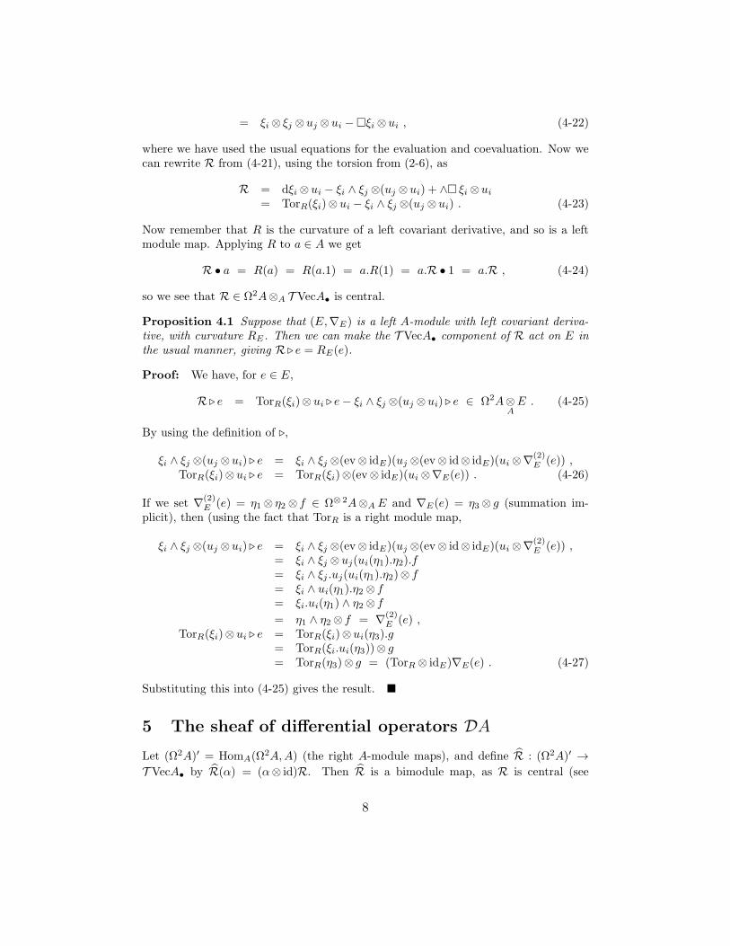
where we have used the usual equations for the evaluation and coevaluation. Now wecan rewrite R from (4-21), using the torsion from (2-6), as

R = dξi ⊗ ui − ξi ∧ ξj ⊗(uj ⊗ui) + ∧ ξi ⊗ui= TorR(ξi)⊗ ui − ξi ∧ ξj ⊗(uj ⊗ui) . (4-23)

Now remember that R is the curvature of a left covariant derivative, and so is a leftmodule map. Applying R to a ∈ A we get

R • a = R(a) = R(a.1) = a.R(1) = a.R • 1 = a.R , (4-24)

so we see that R ∈ Ω2A⊗A T VecA• is central.

Proposition 4.1 Suppose that (E,∇E) is a left A-module with left covariant deriva-tive, with curvature RE. Then we can make the T VecA• component of R act on E inthe usual manner, giving R ⊲ e = RE(e).

Proof: We have, for e ∈ E,

R ⊲ e = TorR(ξi)⊗ ui ⊲ e− ξi ∧ ξj ⊗(uj ⊗ui) ⊲ e ∈ Ω2A⊗AE . (4-25)

By using the definition of ⊲,

ξi ∧ ξj ⊗(uj ⊗ui) ⊲ e = ξi ∧ ξj ⊗(ev⊗ idE)(uj ⊗(ev⊗ id⊗ idE)(ui ⊗∇(2)E (e)) ,

TorR(ξi)⊗ui ⊲ e = TorR(ξi)⊗(ev⊗ idE)(ui ⊗∇E(e)) . (4-26)

If we set ∇(2)E (e) = η1 ⊗ η2 ⊗ f ∈ Ω⊗ 2A⊗AE and ∇E(e) = η3 ⊗ g (summation im-

plicit), then (using the fact that TorR is a right module map,

ξi ∧ ξj ⊗(uj ⊗ui) ⊲ e = ξi ∧ ξj ⊗(ev⊗ idE)(uj ⊗(ev⊗ id⊗ idE)(ui ⊗∇(2)E (e)) ,

= ξi ∧ ξj ⊗ uj(ui(η1).η2).f= ξi ∧ ξj .uj(ui(η1).η2)⊗ f= ξi ∧ ui(η1).η2 ⊗ f= ξi.ui(η1) ∧ η2 ⊗ f

= η1 ∧ η2 ⊗ f = ∇(2)E (e) ,

TorR(ξi)⊗ui ⊲ e = TorR(ξi)⊗ui(η3).g= TorR(ξi.ui(η3))⊗ g= TorR(η3)⊗ g = (TorR ⊗ idE)∇E(e) . (4-27)

Substituting this into (4-25) gives the result.

5 The sheaf of differential operators DA

Let (Ω2A)′ = HomA(Ω2A,A) (the right A-module maps), and define R : (Ω2A)′ →

T VecA• by R(α) = (α⊗ id)R. Then R is a bimodule map, as R is central (see

8

(4-24)). Define W ⊂ T VecA• to be the 2-sided ideal (for the • product) generated by

the image of R, and DA to be the quotient DA = T VecA•/W . We use [v] to denotethe equivalence class in DA containing v ∈ T VecA•.

Recall that T VecA• has a left action, denoted ⊲, on all objects of AE . We wishto consider modules of the quotient DA, and the obvious way to do this is to define[v] ⊲ e = v ⊲ e. However then we have to suppose that W annihilates every e ∈ E, or

equivalently that every element of the image of R annihilates every e ∈ E.

Proposition 5.1 If (E,∇E) has zero curvature, then the formula [v] ⊲ e = v ⊲ e definesan action of DA. Conversely, under the assumption that Ω2A is finitely generatedprojective as a right A-module, if the formula [v] ⊲ e = v ⊲ e defines an action of DA on(E,∇E), then (E,∇E) has zero curvature.

Proof: From Proposition 4.1 we have, for α ∈ (Ω2A)′

(α⊗ id)R ⊲ e = (α⊗ idE)RE(e) ∈ E , (5-28)

so if RE = 0 then the formula gives an action of DA.Conversely, if the finitely generated projective assumption holds and (α⊗ id)RE(e) =

0 for all α ∈ (Ω2A)′, then RE = 0.

If we remember that the left covariant derivative ∇ on T VecA• from (3-14) is

∇(v) = ξi ⊗ui • v , (5-29)

it is obvious that ∇ restricts to the ideal W ⊂ T VecA•, and has a quotient ∇DA onDA. (In fact, we could use any ideal for the • product here.) Explicitly, the covariantderivative is given by

∇DA([v]) = ξi⊗[ui • v] . (5-30)

Proposition 5.2 Suppose that Ω2A is finitely generated projective as a right A-module.Then the curvature RDA of (DA,∇DA) is zero.

Proof: The curvature is given by

RDA([v]) = (d⊗ idD − id ∧ ∇D)∇D([v])= (d⊗ idD − id ∧ ∇D)

(ξi ⊗[ui • v]

)

= dξi⊗[ui • v]− ξi ∧ ξj ⊗[uj • ui • v]=

(dξi ⊗[ui]− ξi ∧ ξj ⊗[uj • ui]

)• [v] . (5-31)

From this, it is enough to show that R ∈ Ω2A⊗A W . If we write the dual basis forΩ2A as φk ⊗αk ∈ Ω2A⊗A(Ω

2A)′ (summed over k), then

R = φk ⊗(αk ⊗ id)R = φk ⊗R(αk) ∈ Ω2A⊗AW .

Example 5.3 Classical differential operators. As R is defined in terms of thecurvature of a connection, it is independent of the choice of dual basis. On an open

9

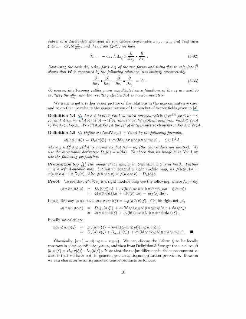
subset of a differential manifold we can choose coordinates x1, . . . , xn, and dual basisξi ⊗ui = dxi ⊗

∂∂xi

, and then from (4-21) we have

R = − dxi ∧ dxj ⊗∂

∂xj•∂

∂xi. (5-32)

Now using the basis dxi ∧ dxj for i < j of the two forms and using this to calculate Rshows that W is generated by the following relations, not entirely unexpectedly:

∂

∂xj•∂

∂xi−

∂

∂xi•

∂

∂xj= 0 . (5-33)

Of course, this becomes rather more complicated once functions of the xi are used tomultiply the ∂

∂xj, and the resulting algebra DA is noncommutative.

We want to get a rather easier picture of the relations in the noncommutative case,and to do that we refer to the generalisation of Lie bracket of vector fields given in [4].

Definition 5.4 [4] An x ∈ VecA⊗VecA is called antisymmetric if ev〈2〉(πx⊗ k) = 0for all k ∈ ker∧ : Ω1A⊗A Ω1A→ Ω2A, where π is the quotient map from VecA⊗VecAto VecA⊗A VecA. We call AntiVec2A the set of antisymmetric elements in VecA⊗VecA.

Definition 5.5 [4] Define ϕ : AntiVec2A→ VecA by the following formula,

ϕ(u⊗ v)(ξ) = Du(v(ξ)) + ev(id⊗ ev⊗ id)(u⊗ v⊗ z) , ξ ∈ Ω1A .

where z ∈ Ω1A⊗A Ω1A is chosen so that ∧z = dξ (the choice does not matter). Weuse the directional derivative Du(a) = u(da). To check that its image is in VecA weuse the following proposition.

Proposition 5.6 [4] The image of the map ϕ in Definition 5.5 is in VecA. Furtherϕ is a left A-module map, but not in general a right module map, as ϕ(u⊗ v).a =ϕ(u⊗ v.a) + u.Dv(a). Also ϕ(u⊗ a.v) = ϕ(u.a⊗ v) +Du(a).v.

Proof: To see that ϕ(u⊗ v) is a right module map use the following, where ∧z = dξ,

ϕ(u⊗ v)(ξ.a) = Du(v(ξ).a) + ev(id⊗ ev⊗ id)(u⊗ v⊗(z.a− ξ⊗da))= ϕ(u⊗ v)(ξ).a + u(v(ξ).da) − u(v(ξ).da) .

It is quite easy to see that ϕ(a.u⊗ v)(ξ) = a.ϕ(u⊗ v)(ξ). For the right action,

ϕ(u⊗ v)(a.ξ) = Du(v(a.ξ)) + ev(id⊗ ev⊗ id)(u⊗ v⊗(a.z + da⊗ ξ))= ϕ(u⊗ v.a)(ξ) + ev(id⊗ ev⊗ id)(u⊗ v⊗ da⊗ ξ) .

Finally we calculate

ϕ(u⊗ a.v)(ξ) = Du(a.v(ξ)) + ev(id⊗ ev⊗ id)(u⊗ a.v⊗ z)= Du(a).v(ξ) +Du.a(v(ξ)) + ev(id⊗ ev⊗ id)(u.a⊗ v⊗ z) .

Classically, [u, v] = ϕ(u⊗ v − v⊗ u). We can choose the 1-form ξ to be locallyconstant in some coordinate system, and then from Definition 5.5 we get the usual result[u, v](ξ) = Du(v(ξ))−Dv(u(ξ)). Note that the major difference in the noncommutativecase is that we have not, in general, got an antisymmetrisation procedure. Howeverwe can characterise antisymmetric tensor products as follows:

10

Proposition 5.7 Suppose that Ω1A and Ω2A are finitely generated projective as rightA-modules, with a dual basis ξi ⊗ui ∈ Ω1A⊗A VecA. Then the subset of all x inVecA⊗A VecA for which ev〈2〉(x⊗ k) = 0 for all k ∈ ker∧ : Ω1A⊗A Ω1A→ Ω2A is

α(ξi ∧ ξj)uj ⊗ ui : α ∈ HomA(Ω

2A,A).

Proof: We have a short exact sequence of right modules,

0 −→ ker∧ −→ Ω1A⊗AΩ1A

∧−→ Ω2A −→ 0 ,

where Ω2A is finitely generated projective as a right A-module. We deduce that thereis a splitting map S : Ω2A → Ω1A⊗A Ω1A. Given x so that ev〈2〉(x⊗ k) = 0 for allk ∈ ker∧, we get a well defined map ω 7→ ev〈2〉(x⊗S(ω)) in HomA(Ω

2A,A). The mapα ∈ HomA(Ω

2A,A) arises in this way from x = α(ξi∧ξj)uj ⊗ui. Any x correspondingto α = 0 would have to be zero on all of Ω1A⊗A Ω1A, i.e. x = 0.

Proposition 5.8 For α ∈ HomA(Ω2A,A),

(α⊗ id)R = ϕ(α(ξi ∧ ξj)uj ⊗ui)− α(ξi ∧ ξj)uj • ui

Proof: Given α ∈ HomA(Ω2A,A), from (4-23) we have

(α⊗ id)R = α(TorR(ξi))ui − α(ξi ∧ ξj)uj ⊗ ui . (5-34)

By the usual evaluation and coevaluation properties, α(ξi ∧ ξj)uj ⊗ui ∈ AntiVec2A(see Definition 5.4). Then, for η ∈ Ω1A, and ∧z = dη,

ϕ(α(ξi ∧ ξj)uj ⊗ ui)(η) = α(ξi ∧ ξj)(Duj

(ui(η)) + ev〈2〉(uj ⊗ui⊗ z))

= α(ξi ∧ ξj)Duj(ui(η)) + α(dη) . (5-35)

We expand the Duj(ui(η)) term using ,

ϕ(α(ξi ∧ ξj)uj ⊗ui)(η) = α(ξi ∧ ξj)((ev⊗ ev)(uj ⊗ui⊗ η)

+ev〈2〉(uj ⊗ui⊗η))+ α(dη)

= α(ξi ∧ ξj) (ev⊗ ev)(uj ⊗ui⊗ η)+α(∧η) + α(dη)

= α(ξi ∧ ξj) (ev⊗ ev)(uj ⊗ui⊗ η) + α(TorR(η)) .(5-36)

This gives

ϕ(α(ξi ∧ ξj)uj ⊗ ui) = α(ξi ∧ ξj) (ev⊗ id)(uj ⊗ui) + α(TorR(ξi))ui ,(5-37)

and on substitution in (5-34) we get

(α⊗ id)R = ϕ(α(ξi ∧ ξj)uj ⊗ui)− α(ξi ∧ ξj) (ev⊗ id)(uj ⊗ui)− α(ξi ∧ ξj)uj ⊗ ui

= ϕ(α(ξi ∧ ξj)uj ⊗ui)− α(ξi ∧ ξj)uj • ui .

Corollary 5.9 Suppose that Ω1A and Ω2A are finitely generated projective as rightA-modules. Then the relations in DA are of the form ϕ(u⊗ v)−u•v for every u⊗ v ∈VecA⊗A VecA (summation implicit) so that ev〈2〉(u⊗ v⊗ k) = 0 for all k ∈ ker∧ :Ω1A⊗A Ω1A→ Ω2A.

Proof: Propositions 5.8 and 5.7. Note that the relation depends only on u⊗ v ∈VecA⊗A VecA, with emphasis on the ⊗A. This is as, by Proposition 5.6, the contri-butions from the two terms cancel when applied to u.a⊗ v − u⊗a.v.

11

6 Example: Differential calculi on Hopf algebras

The idea of these calculi follows from [29]. For a Hopf algebra H with a left covariantdifferential calculus, there is a well defined left coaction λ : Ω1H → H ⊗Ω1H definedby λ(x.dy) = x(1) y(1) ⊗x(2).dy(2). We write λ(ξ) = ξ[−1] ⊗ ξ[0]. Set L1H to be thecoinvariants under the left coaction, i.e. those ξ ∈ Ω1H so that λ(ξ) = 1⊗ ξ. If theantipode S is invertible, there is an isomorphism Ω1H ∼= L1H ⊗H , given by productone way, and the other way by ξ 7→ ξ[0].S

−1(ξ[−1])⊗ ξ[−2]. If Ω1H is finitely generated

as a right H-module, then L1H is a finite dimensional vector space. There is a leftaction of H on L1H given by h ⊲ η = h(2) η S

−1(h(1)). The product of a element of Hon the left with an element of Ω1H ∼= L1H ⊗H is given by h.(ξ⊗ g) = h(2) ⊲ ξ⊗h(1) g.

If we set h to be the vector space dual of L1H , then VecH ∼= H ⊗ h, where thepairing between VecH and Ω1H is given by (h⊗α)(ξ⊗ g) = hα(ξ) g ∈ H . We takeξi ⊗ui ∈ L1H ⊗ h (summing over i) to be a dual vector space basis. Now from (4-21)

R = dξi ⊗ui − ξi ∧ ξj ⊗uj • ui . (6-38)

Now take a vector space basis ωk of the left invariant 2-forms, and (summing over k)

dξi = nik ωk , ξi ∧ ξj = eijk ωk . (6-39)

The relations in DA are then

nik ui = eijk uj • ui . (6-40)

Further analysis of this for functions on a Lie group would give the classical Lie algebra(i.e. h) structure constants.

For a noncommutative example, we will give the relations for the 3D calculus onquantum SU2 (see [29] for the original work, and [3] for our notation). There is a basise0, e+, e− for the left invariant 1-forms, and we then have:

de0 = q3e+ ∧ e−, de± = ∓ q±2 (1 + q−2) e± ∧ e0, e± ∧ e± = e0 ∧ e0 = 0

q2e+ ∧ e− + e− ∧ e+ = 0, e0 ∧ e± + q±4 e± ∧ e0 = 0

We now set ω0 = e+ ∧ e− and ω± = e± ∧ e0, and take u0, u± to be the dual basis ofe0, e+, e− (i.e. ui(e

j) = δij). Now the coefficients in (6-39) are given by eiik = 0 and

n0k =

q3 k = 00 otherwise

, n±k =

∓ q±2 (1 + q−2) k = ±

0 otherwise,

e±0k =

1 k = ±0 otherwise

, e0±k =

−q±4 k = ±0 otherwise

,

e+−k =

1 k = 00 otherwise

, e−+k =

−q2 k = 00 otherwise

.

This gives the relations in DA,

q3 u0 = u− • u+ − q2 u+ • u− ,

12

∓ q±2 (1 + q−2)u± = u0 • u± − q±4 u± • u0 . (6-41)

In [3] it is shown that the only left invariant left covariant derivatives on the 3DΩ1

Cq[SU2] which are bimodule covariant derivatives, and are invariant under the rightCZ coaction are of the form (6-42) (where we use ∇L for the restriction to the leftinvariant forms). Note we have set ν = µ+, µ = µ− compared to the notation in [3],and assume that q is not a root of unity.

∇L(e0) = r e0 ⊗ e0 + µ+ e+⊗ e− + µ− e

−⊗ e+ ,∇L(e±) = n± e

0 ⊗ e± +m± e± ⊗ e0 . (6-42)

Proposition 6.1 The curvature of the connection in (6-42) is (summing over the ±in the second formula)

R(e±) =(n± q

3e+ ∧ e− − µ∓m± e± ∧ e∓

)⊗ e±

+m±

(∓ q±2 (1 + q−2) + n± q

±4 − r)e± ∧ e0 ⊗ e0 ,

R(e0) =(r q3 − µ+m− + µ−m+ q

2)e+ ∧ e−⊗ e0

+µ±

(∓ q±2 (1 + q−2) + r q±4 − n∓

)e± ∧ e0 ⊗ e∓ .

Proof: From the definition of curvature,

R(e±) = n± de0 ⊗ e± +m± de± ⊗ e0

−n± e0 ∧∇L(e±)−m± e

± ∧ ∇L(e0)= n± q

3e+ ∧ e− ⊗ e± ∓m± q±2 (1 + q−2) e± ∧ e0⊗ e0

−n±m± e0 ∧ e± ⊗ e0 −m± e

± ∧ (r e0 ⊗ e0 + µ∓ e∓⊗ e±)

=(n± q

3e+ ∧ e− − µ∓m± e± ∧ e∓

)⊗ e±

+m±

(∓ q±2 (1 + q−2) e± ∧ e0 − n± e

0 ∧ e± − r e± ∧ e0)⊗ e0

=(n± q

3e+ ∧ e− − µ∓m± e± ∧ e∓

)⊗ e±

+m±

(∓ q±2 (1 + q−2) + n± q

±4 − r)e± ∧ e0 ⊗ e0 .

Summing over the ± in the following formula,

R(e0) = r de0 ⊗ e0 + µ± de± ⊗ e∓

−r e0 ∧ ∇L(e0)− µ± e± ∧ ∇L(e∓)

= r q3e+ ∧ e−⊗ e0 ∓ µ± q±2 (1 + q−2) e± ∧ e0 ⊗ e∓

−r µ± e0 ∧ e±⊗ e∓ − µ± e

± ∧ (n∓ e0 ⊗ e∓ +m∓ e

∓ ⊗ e0)=

(r q3e+ ∧ e− − µ± e

± ∧m∓ e∓)⊗ e0

+µ±

(∓ q±2 (1 + q−2) e± ∧ e0 − r e0 ∧ e± − n∓ e

± ∧ e0)⊗ e∓ .

Corollary 6.2 The left covariant derivative in (6-42) has zero curvature in preciselyfour cases:a) ∇L = 0.b) n− = − q2 (1 + q−2) = −µ+m− q

−1 , n+ = q−2 (1 + q−2) = q−3 µ−m+ , r = 0.c) n− = m− = µ+ = 0 , n+ = q−2 = q−3 µ−m+ , r = −1.d) n+ = m+ = µ+ = 0 , n− = − 1 = −µ+m− q

−1 , r = q−2.Generically, all these cases have invertible σ.

13

From Corollary 6.2 and [3], the only curvature zero case where σ satisfies the braidrelations is the trivial case ∇L = 0. However we do find the following statement aboutthe star operation ⋆ : Ω1H → Ω1H given by the star operation on quantum SU2, whichassumes that q is real.

Corollary 6.3 The condition that the zero curvature left covariant derivative in Corol-lary 6.2 preserves the star operation in the sense that

(id⊗ ⋆)∇Ω1H = ∇Ω1H⋆

is that we have case (a) of Corollary 6.2, or the sub-case of (b) where

m+ = −m∗− , µ+ = − q2 µ∗

− , −µ−m∗− = q + q−1 .

Proof: Substitute the cases of Corollary 6.2 into the equations of [3].

Now we take the basis order e+, e0, e− for L1H , and write matrices to give theaction of the ui, by right multiplication on column vectors:

u+ →

0 0 0m+ 0 00 µ+ 0

, u0 →

n+ 0 00 r 00 0 n−

, u− →

0 µ− 00 0 m−

0 0 0

.(6-43)

This is just read off (6-42). However we can now check our calculations by substitutingthese matrices into the relations in (6-41). This gives the following series of equations,which is precisely the same as the conditions for zero curvature in Corollary 6.2:

m+ µ− = n+q3 , m− µ+ −m+ µ−q

2 − q3r = 0 , m−µ+ = −n−qm+(−1− q2 + n+q

4 − r) = 0 , µ+(1 + n− + q2 − q4r) = 0 ,µ−(−1− q2 + n+q

4 − r) = 0 , m−(1 + n− + q2 − q4r) = 0 . (6-44)

Why did we only have to look at the n-forms to get the relations (6-41), and thenhave to do lots of hard work to find the curvature? The construction of the algebraDA and its actions was very explicit, and involves specifying covariant derivatives.However it turns out that many of the relations on DA, viewed as an algebra generatedby elements of VecA, do not depend on specifying covariant derivatives. But there are,in general, other relations in DA – a choice of dual basis of VecA still leaves relationsbetween the basis elements (for a non-freely generated case, the Hopf algebra case isfreely generated). We do not claim to have studied the properties of DA as an abstractalgebra, and it might be interesting to do so.

7 The crossing map for DA

Definition 7.1 The categories AF and AFA are defined exactly as AE and AEA in Def-inition 2.1, except that we require that the curvature of the left derivative vanishes forboth, and for (E,∇E , σE) in AFA we require the existence of a map σE : E⊗A Ω2A→Ω2A⊗AE so that, on E⊗A Ω1A⊗A Ω1A

σE(idE ⊗∧) = (∧⊗ idE)(id⊗σE)(σE ⊗ id) . (7-45)

14

Note that if Ω2A is finitely generated projective as a right A-module, then (7-45)implies the existence of σ−1

E : (Ω2A)′ ⊗AE → E⊗A(Ω2A)′ so that

(idE ⊗ ev)(σ−1E ⊗ id) = (ev⊗ idE)(id⊗ σE) : (Ω

2A)′ ⊗AE⊗

AΩ2A→ E . (7-46)

In Section 3, summarising the results of [2], we stated that (T VecA•,∇, 0), withthe left bimodule covariant derivative given in (3-14), was in the center of the cate-gory AEA, using the crossing natural transformation ϑ. In Section 5 we showed (un-der the condition that Ω2A is finitely generated projective as a right A-module) that(DA,∇D , 0) is in AFA. We also showed that DA acts on objects in AF . It is naturalto ask if (DA,∇D , 0) is in the center of AFA, and to see if the original crossing natural

transformation ϑ, defined in (3-15) and (3-16), is compatible with the relations R(α).

Proposition 7.2 Suppose that for (E,∇E , σE) ∈ AEA, (7-45) holds, that Ω2A isfinitely generated projective as a right A-module, and that the curvature RE : E →Ω2A⊗AE is a right module map. Then

ϑE (R⊗ idE) = R ⊲ idE ⊗ 1A + (ev⊗ idE ⊗ id)(id⊗ σE ⊗R)(id⊗ idE ⊗ coev2): (Ω2A)′ ⊗

AE → E⊗

AT VecA .

where coev2(1) ∈ Ω2A⊗A(Ω2A)′ is the dual basis for Ω2A.

Proof: First, from (3-15) and (3-16), for α ∈ (Ω2A)′ and e ∈ E,

ϑE((α⊗ id)R⊗ e) = α(dξi)ϑE(ui⊗ e)− α(ξi ∧ ξj)ϑE(uj • ui⊗ e)= α(dξi)ϑE(ui⊗ e)−

α(ξi ∧ ξj) (⊲⊗ id + σ−1E • id)(uj ⊗ϑE(ui⊗ e))

= α(dξi) (ui ⊲ e+ σ−1E (ui ⊗ e))−

α(ξi ∧ ξj) (⊲⊗ id + σ−1E • id)(uj ⊗(ui ⊲ e+ σ−1

E (ui⊗ e))) ,

and from this we have

ϑE((α⊗ id)R⊗ e)− (α⊗ id)R ⊲ e⊗ 1A= α(dξi)σ

−1E (ui⊗ e)− α(ξi ∧ ξj)σ

−1E (uj ⊗(ui ⊲ e))−

α(ξi ∧ ξj) (⊲⊗ id + σ−1E • id)(uj ⊗ σ−1

E (ui ⊗ e)) . (7-47)

In (7-47) the actions are made of u ⊲ e = (ev⊗ idE)(u⊗∇Ee), and these can be com-bined with the coevaluations coev(1) = ξi ⊗ ui to simplify certain of the terms, asfollows. Counting multiplying out the brackets, we have four terms on the RHS of(7-47), and then the second and third terms give

α(ξi ∧ ξj)σ−1E (uj ⊗(ui ⊲ e)) = (α⊗σ−1

E )(id ∧ coev⊗ idE)∇E(e)= (α⊗ idE ⊗ id)(id ∧ σE ⊗ id)(∇E(e)⊗ ξi ⊗ ui) ,

α(ξi ∧ ξj) (uj ⊲ σ−1E (ui⊗ e)) = (α⊗ idE ⊗ id)(id ∧ ∇E ⊗ id)(ξi ⊗ σ−1

E (ui ⊗ e)) .

The fourth term of (7-47) gives (using the definition of •)

α(ξi ∧ ξj) (σ−1E • id)(uj ⊗σ−1

E (ui⊗ e))= (α ∧ ⊗ idE ⊗ id⊗ 2)(id⊗σE ⊗ id⊗ 2)(σE ⊗ id⊗ 3)(e⊗ ξi ⊗ ξj ⊗uj ⊗ ui)+

15

(α ∧ ⊗ idE ⊗ id)(id⊗ σE ⊗ id)(id⊗ idE ⊗)(ξi ⊗ σ−1E (ui ⊗ e)) . (7-48)

We shall call the two terms of the RHS of (7-48) terms 4a and 4b respectively of (7-47).Then combining terms 1,3 and 4b gives

(α⊗ idE ⊗ id)(d⊗ idE ⊗ id− id ∧ ∇E ⊗ id− id ∧ (σE ⊗ id)(idE ⊗)

)

(ξi ⊗σ−1E (ui⊗ e))

= (α⊗ idE ⊗ id)(d⊗ idE ⊗ id− id ∧ ∇E ⊗ id− id ∧ (σE ⊗ id)(idE ⊗)

)

(σE(e⊗ ξi)⊗ui) , (7-49)

where we have used the fact that the long bracket gives a well defined operator onΩ1A⊗AE⊗AVecA. Now we can rewrite (7-48) as

ϑE((α⊗ id)R⊗ e)− (α⊗ id)R ⊲ e⊗ 1A

= − (α⊗ idE ⊗ id)((id ∧ σE ⊗ id⊗ 2)(σE ⊗ id⊗ 3)(e⊗ ξi ⊗ ξj ⊗ uj ⊗ ui)

+((d⊗ idE − id ∧∇E)σE ⊗ id− (id ∧ σE)(∇E ⊗ id)⊗ id−

(id ∧ (σE ⊗ id)

)(σE ⊗)

)(e⊗ ξi ⊗ ui)

)(7-50)

Now we use the following equality, which is proved in [1] for vanishing curvature, butin fact the proof only requires that the curvature RE is a right A-module map.

(d⊗ idE − (id ∧ ∇E)

)σE = (id ∧ σE)(∇E ⊗ id) + σE(idE ⊗d) : E⊗

AΩ1A→ Ω2A⊗

AE .

We can use this to rewrite (7-50) as

ϑE((α⊗ id)R⊗ e)− (α⊗ id)R ⊲ e⊗ 1A

= − (α⊗ idE ⊗ id)((id ∧ σE ⊗ id⊗ 2)(σE ⊗ id⊗ 3)(e⊗ ξi ⊗ ξj ⊗ uj ⊗ ui)

+(σE(idE ⊗ d)⊗ id−

(id ∧ (σE ⊗ id)

)(σE ⊗)

)(e⊗ ξi ⊗ui)

)

= ((α⊗ idE)σE ⊗ id)(e⊗ dξi ⊗ui − e⊗ ξi ∧ ξj ⊗uj • ui) . (7-51)

Now using (7-46) gives the answer.

Corollary 7.3 Suppose that (E,∇E , σE) ∈ AFA , and that Ω2A is finitely generatedprojective as a right A-module. Then

ϑE(W ⊗AE) ⊂ E⊗

AW ,

and as a result we have a well defined quotient ϑE : DA⊗AE → E⊗A DA.

Proof: From Proposition 7.2, since R ⊲ idE = 0, we have

ϑE (R⊗ idE) = (ev⊗ idE ⊗ id)(id⊗ σE ⊗R)(id⊗ idE ⊗ coev2): (Ω2A)′ ⊗

AE → E⊗

AT VecA .

To get the result for the ideal under the • product, we use the multiplicative propertyof ϑE listed in (3-17).

16

8 Differential operators with module endomorphisms

We would like to consider vector fields acting on left modules E with left covariantderivative ∇E , together with left module endomorphisms (in AEnd(E)) acting on E.For example, the classical Dirac operator acting on sections of the spinor bundle re-quires such a module map. There are at least two reasons why this is not really enough.The first is that we would prefer to be able to reorder vector fields and left modulemaps, rather than leave them in some sort of free product. To see what happens whenwe do this, we use the following lemma, where stands for composition of functions:

Lemma 8.1 Given (E,∇E) ∈ AE and T ∈ AEnd(E), we have a left module map∇(T ) : E → Ω1A⊗AE defined by ∇(T ) = ∇ T − (id⊗T ) ∇.

Proof: Consider ∇(a.T ) for a ∈ A.

Now we have, for T ∈ AEnd(E) and u ∈ VecA,

((u ⊲) T − T (u ⊲)

)(e) = (ev⊗ idE)(u⊗∇(T )(e)) . (8-52)

Starting from a left module map from E to E, we end up introducing a module mapfrom E to Ω1A⊗AE. But there is another reason why we may wish to consider suchmaps. If we were to start only with the module E, it might be considered as ratherartificial to impose one particular covariant derivative on it. The difference betweenany two covariant derivatives is a left module map from E to Ω1A⊗AE. If we add suchmodule maps from the beginning, we obtain actions on E which are independent of thechoice of covariant derivative on E. For these reasons, we make the following definition.For a left module map S : E → Ω⊗nA⊗AE and v ∈ Vec⊗nA define Kn(v, S) : E → Eby

Kn(v, S)(e) = (ev〈n〉⊗ idE)(v⊗S(e)) . (8-53)

Now (8-52) reads (u ⊲) T − T (u ⊲) = K1(u,∇(T )). For completeness we defineK0(a, T ) = a.T . To see how these operations combine, we define, for S : E →Ω⊗nA⊗AE and U : E → Ω⊗mA⊗AE,

S U = (id⊗m ⊗S)U : E → Ω⊗m+nA⊗AE . (8-54)

Now we have

Kn(v, S) Km(w,U) = Kn+m(v⊗w, S U) . (8-55)

To look at the other compositions, we will need to observe that, using (2-5),

∇E(S) = (〈n〉 ⊗ idE + id⊗n ⊗∇E)S − (σ−〈n〉 ⊗ idE)(id⊗S)∇E . (8-56)

is a left module map ∇E(S) : E → Ω⊗n+1A⊗AE. To complete being able to reorderthe Kn to the left and the ⊲ to the right we need the following result:

17

Proposition 8.2 For u ∈ VecA, v ∈ Vec⊗nA and S : E → Ω⊗nA⊗AE,

(u ⊲) Kn(v, S) = Kn(u ⊲ v, S) +Kn+1(u⊗ v,∇E(S)) +Kn(v′, S) (u′ ⊲) ,

where σ−〈n〉(u⊗ v) = v′ ⊗u′ (a finite sum) and σ−〈n〉 : Vec⊗n+1A → Vec⊗n+1A isgiven by the same symbolic formula as (2-5), though the domain is different.

Proof: By differentiating the evaluation and using (8-56) we have

(u ⊲) Kn(v, S)(e) = Kn(u ⊲ v, S)+ (ev〈n+1〉 ⊗ idE)((u⊗ v)⊗(〈n〉⊗ idE + id⊗n ⊗∇E)S(e))

= Kn(u ⊲ v, S) +Kn+1(u⊗ v,∇E(S))+ (ev〈n+1〉 ⊗ idE)((u⊗ v)⊗(σ−〈n〉 ⊗ idE)(id⊗S)∇E(e)) .

9 Symbols of differential operators

The reader will recall that classically the symbol is made from the highest order partof the differential operator. The partial derivatives are replaced by the correspondingvectors, and we get a section of some tensor power of the tangent space. Of course,we could take all orders instead of just the highest order, but then we would find thatthe lower order terms were coordinate dependent. The symbols have useful properties:When we compose differential operators, we take the tensor product of their symbols.Some classes of differential operators, most famously elliptic operators, have much oftheir behaviour determined by their symbols.

It will now not surprise the reader that the basic idea of symbols and the com-position rule work in the noncommutative setting. After all, we have been describingdifferential operators by taking tensor powers of vector spaces to all orders. Merelyrestricting to the highest order non-zero term gives the symbol. A look at Lemma 3.1shows that composition of differential operators using the • product is simply ⊗A onthe highest order parts. Of course the lower order terms of the • product depend onthe covariant derivative – changing this covariant derivative is effectively changingcoordinates.

However we need to be careful - the symbol is classically an element of a symmetrictensor product, or equivalently expressed as a (commutative) polynomial. What wehave been saying in a noncommutative context refers to T VecA• – the full tensorproduct which acts on the category AE . In Section 5 we discuss the algebra DAwhich has extra relations imposed, and acts on modules with zero curvature covariantderivative AF . Now these relations, taking only the highest tensor order part, applyto the symbols. For example, for the 3D calculus on deformed SU(2) discussed inSection 6, from (6-41) we get following relations

u− ⊗u+ − q2 u+ ⊗u− = 0 , u0 ⊗u± − q±4 u± ⊗u0 = 0 . (9-57)

Then a symbol for D for this calculus really is a polynomial in u0, u+, u−, with therelatively minimal change in product (9-57) from the classical case (taking coefficientsin the algebra, if the differential operator is not left invariant). However it may be thatwe were lucky in this case – more generally it might be possible that the relations onDA might have combinations cancelling in order 2, producing non-obvious relations inorder 1. Caution is advised until the situation is understood better.

18

10 Noncommutative complex structures

We shall use the version of noncommutative complex differential geometry introducedin [5] and referenced in [18]. Suppose that A is a star algebra with differential calculusfor which the map a.db 7→ db∗.a∗ gives a well defined star operation on Ω1A, extendingto all ΩnA. Then an almost complex structure on A is a bimodule map J : Ω1M →Ω1M for which J(ξ∗) = J(ξ)∗, J J is minus the identity, and the map

J ⊗ id⊗n−1 + · · ·+ id⊗n−1 ⊗ J : Ω⊗nA→ Ω⊗nA (10-58)

gives a well defined map (via the ∧ product) J : ΩnA → ΩnA. From this we candecompose each ΩnA into a direct sum of Ωp,qA, the i (p−q) eigenspace of J , where p+q = n and p, q ≥ 0. Take πp,q : ΩnA→ Ωp,qA to be the corresponding projection. Thealmost complex structure is called integrable if (amongst several equivalent conditions),for all ξ ∈ Ω0,1A we have dξ ∈ Ω0,2A⊕ Ω1,1A.

The idea of complex structure given here is exactly the same as that used in commu-tative geometry – though the star condition is ommitted as in an a priori real manifold,it is not needed. Also the integrability condition is more often given in terms of vectorfields, and we will come to this below. Now the content of the Newlander-Nirenbergintegrability theorem [24] is that on a real manifold, with an almost complex struc-ture satisfying the integrability condition, we can construct local complex coordinates,linked by complex analytic transition functions.

However we do not really know what a noncommutative ‘real manifold’ is, and(at least with our current degree of understanding) we cannot use the idea of localcoordinates. It is tempting to believe that there would be an analogue of the Newlander-Nirenberg integrability theorem in the noncommutative case, but what would replacelocal coordinates? In this paper I shall make an argument that we should look atcovariant derivatives on the 1-forms with certain properties as a substitute for localcomplex coordinates.

To deal with a few more tecnicalities and matters of notation, if ΩnA is a finitelygenerated projective module, then so are the Ωp,qA for p + q = n, as they sum toΩnA. We define ∂ : Ωp,qA → Ωp+1,qA and ∂ : Ωp,qA → Ωp,q+1A by d followed by theappropriate projection, πp+1,q or πp,q+1. By the integrability condition, ∂2 = 0 and∂2 = 0.

As the vector fields are dual to the 1-forms (i.e. VecA = HomA(Ω1A,A)), many

things that can be done with one can be done with the other. In particular I mentionedthat the original approach to the Newlander-Nirenberg integrability theorem was viavector fields. Just to show that it can be done in a noncommutative setting, we shallnow show that the integrability condition can be phrased in terms of vector fields.Remember that Definition 5.5 gives our form of the Lie bracket of vector fields:

Definition 10.1 For an almost complex structure J : Ω1A→ Ω1A, define J : VecA→VecA by J(v) = v J . Then the ±i eigenspaces of J are respectively denoted Vec1,0Aand Vec0,1A.

Proposition 10.2 The Newlander-Nirenberg integrability condition. Supposethat the integrability condition holds for an almost complex structure on Ω1A. Also

19

suppose that x ∈ Vec1,0A⊗Vec1,0A obeys the condition that ev〈2〉(x⊗ k) = 0 for allk ∈ ker∧ : Ω1,0A⊗AΩ1,0A→ Ω2,0A. Then ϕ(x) ∈ Vec1,0A.

Proof: Write x = u⊗ v (summation implicit). We ned to show that ϕ(u⊗ v)(ξ) = 0for all ξ ∈ Ω0,1A. The formula is, where z ∈ Ω1A⊗A Ω1A is chosen so that ∧z = dξ,

ϕ(X ⊗Y )(ξ) = Du(v(ξ)) + ev〈2〉(u⊗ v⊗ z) ,

Now Y (ξ) = 0, so we only have to show that ev〈2〉(u⊗ v⊗ z) = 0. As ξ ∈ Ω0,1A, thedifferential form version of the integrability condition states that dξ ∈ Ω0,2A⊕Ω1,1A.This means that we can choose not to have any component of z in Ω1,0A⊗A Ω1,0A, soev〈2〉(u⊗ v⊗ z) = 0.

11 What is a holomorphic vector field?

Classically, if we differentiate a holomorphic function along a holomorphic vector field,we should get another holomorphic function. In terms of local holomorphic coordinatesz1, . . . , zn, the following is a holomorphic vector field, where the functions fi(z1, . . . , zn)are holomorphic functions,

v = f1(z1, . . . , zn)∂

∂z1+ · · ·+ fn(z1, . . . , zn)

∂

∂zn. (11-59)

However in noncommutative geometry we do not have the luxury of working in localcoordinates, we need a global definition.

A glance at (11-59) will show that v ∈ Vec1,0A (see Definition 10.1). Now sup-pose that v ∈ Vec1,0A and a ∈ A is holomorphic, i.e. ∂ a = 0. The differential of aalong (or in the direction of) v is ev(v⊗da). For this to be holomorphic, we need∂ ev(v⊗da) = 0. In terms of the projection π0,1 we have π0,1 d ev(v⊗da) = 0. (Weremind the reader that πp,q is the projection from Ωp+qA to Ωp,qA.) Classically, we per-form this differentiation in the given coordinates, and see that the functions f1, . . . , fnmust be holomorphic. Next we say that, since the change of coordinate functions areholomorphic, it makes sense to say that the corresponding functions are holomorphicin every coordinate chart. Of course, we can’t do any of this. We have to differentiatethe vector field with the only tool we have for doing this, a covariant derivative. Whenwe do this, we not surprisingly discover that there are additional conditions that wemust impose on the covariant derivative, and these conditions stand in for the classicalassumption that the change of coordinate functions are holomorphic.

To differentiate ev(v⊗da) use the covariant derivatives from (2-7), and write

π0,1 d ev(v⊗ da) = (π0,1 ⊗ ev)( v⊗da) + (ev⊗π0,1)(v⊗ da) . (11-60)

Before continuing, it would be wise to review the meaning of (11-60). In fact, itmay contain no information at all. On a compact complex manifold, all holomorphicfunctions are constants, and (11-60) becomes 0 = 0 + 0, independently of v. What weare going to do is to obtain a condition which is more local in character, and whichwould imply ev(v⊗da) holomorphic for any holomorphic a.

20

Lemma 11.1 Suppose thata) ∧ : Ω1,0A⊗A Ω0,1A→ Ω1,1A is an isomorphism with inverse φ,b) (J ⊗ id) = J : Ω1A→ Ω1A⊗A Ω1A,c) π1,1TorR : Ω1A→ Ω1,1A vanishes.Then we have, for v ∈ Vec1,0A and a ∈ A,

π0,1 d ev(v⊗ da) = (π0,1 ⊗ ev)( v⊗ ∂a)− (ev⊗ id)(v⊗φπ1,1 ∧ ∂a) .

Proof: To repeat (11-60), for v ∈ Vec1,0A and a ∈ A,

π0,1 d ev(v⊗da) = π0,1 d ev(v⊗ ∂a)= (π0,1 ⊗ ev)( v⊗ ∂a) + (ev⊗π0,1)(v⊗ ∂a) .

By (b)

∂a = (id⊗π0,1) ∂a+ (id⊗π1,0) ∂a ∈ Ω1,0A⊗AΩ0,1A

⊕Ω1,0A⊗

AΩ1,0A .

From this it follows that, where φ is the inverse of ∧ : Ω1,0A⊗A Ω0,1A→ Ω1,1A.

π1,1 ∧ ∂a = ∧(id⊗π0,1) ∂a ,φ π1,1 ∧ ∂a = (id⊗ π0,1) ∂a ,

Now remember the definition (2-6) of TorR, and using the fact that d2a = 0 we get

0 = π1,1TorR(da) = π1,1 ∧ da = π1,1 ∧ ∂a+ π1,1 ∧ ∂a ,

giving (id⊗ π0,1) ∂a = −φπ1,1 ∧ ∂a and the result.

Corollary 11.2 Given the conditions of Lemma 11.1, if (π0,1 ⊗ id) v = 0 for v ∈Vec1,0A, it follows that if a ∈ A is holomorphic, then so is ev(v⊗da).

Returning to the conditions of Proposition 11.1 from the point of view of examples,it is instructive to note the assumption that ∧ : Ωp,0A⊗A Ω0,qA → Ωp,qA is an iso-morphism is not only true for the noncommutative complex projective spaces in [25],but that the assumption is fundamental to the whole construction there. Of course,classically condition (a) is just reordering wedge products of coordinate functions usingdzi ∧ dzj = −dzj ∧ dzi.

12 Nice covariant derivatives on integrable complex

structures

To review Section 11, we should ask why the conditions on in Lemma 11.1 arerequired. It should be remembered that the form of the holomorphic vector fieldin (11-59) and its behaviour is completely determined by our idea of local complexcoordinates in the classical case. In the noncommutative setting we lose this, and allwe have to replace it is . In other words, needs to contain all the informationabout the local complex coordinates, and their analytic transition functions, that we

21

need to complete the proof. From this point of view, it is not surprising that

will be subject to various conditions, as it is basically encoding much of the idea ofa ‘noncommutative complex manifold’. To continue the discussion from Section 10,the conditions of Lemma 11.1 might form part of what replaces ‘local holomorphiccoordinates’ in noncommutative geometry. It is possible to go part way to building a‘nice’ covariant derivative that has these properties, as follows.

To begin, remember that any finitely generated projective right A-module E canbe given a right covariant derivative ∇ : E → E⊗A Ω1A. Given a dual basis ei ∈ Eand ei ∈ HomA(E,A), define ∇(ei) = ej ⊗Γji where we consider Γji as a matrixwith entries in Ω1A. The relations between the ei are given by ei Pij = ej, wherePij = ei(ej) is a projection matrix with values in A. Without loss of generality we may

assume that P Γ = Γ (using the matrix product). Applying ∇ to the relation gives therequired equation P Γ (1− P ) = P.dP . This has solutions Γ = P.dP +PBP , where Bis any matrix with entries in Ω1A. Of course, constructing a right bimodule covariantderivative is more complicated, if it is possible at all.

Now Ω1,0A and Ω0,1A are direct summands of Ω1A, so if Ω1A is right finitely gen-erated projective it follows that both Ω1,0A and Ω0,1A are also right finitely generatedprojective. We shall suppose that we are given right bimodule covariant derivatives∇10 : Ω1,0A → Ω1,0A⊗A Ω1A and ∇01 : Ω0,1A → Ω0,1A⊗A Ω1A, with correspondingσ−110 and σ−1

01 . It might be possible to further assume that ∇10 and ∇01 are linked by

conjugation ⋆ : Ω1,0A→ Ω0,1A, but we shall not be concerned by this now. What doesconcern us is that we can construct a right bimodule covariant derivative on Ω1A justby adding the ones on Ω1,0A and Ω0,1A. However we shall modify ∇10 and ∇01 first.

Proposition 12.1 Suppose that we have right bimodule covariant derivatives (Ω1,0A,∇10, σ−110 )

and (Ω0,1A,∇01, σ−101 ). We suppose that

a) ∧ : Ω1,0A⊗A Ω0,1A→ Ω1,1A is an isomorphism with inverse φ,b) ∧ : Ω0,1A⊗AΩ1,0A→ Ω1,1A is an isomorphism with inverse ψ.Then there is a right bimodule covariant derivative (Ω1A,, σ−1) defined by

=((id⊗π1,0)∇10 − φπ1,1d

)π1,0 +

((id⊗π0,1)∇01 − ψ π1,1d

)π0,1 ,

σ−1 =((id⊗π1,0)σ−1

10 − φπ1,1 ∧)(id⊗ π1,0) +

((id⊗π0,1)σ−1

01 − ψ π1,1 ∧)(id⊗π0,1) .

Further (Ω1A,, σ−1) satisfies the properties:i) (J ⊗ id) = J : Ω1A→ Ω1A⊗A Ω1A,ii) π1,1TorR : Ω1A→ Ω1,1A vanishes.iii) π1,1 ∧ σ−1 = − π0,1 ∧ π1,0 − π1,0 ∧ π0,1 : Ω⊗ 2A→ Ω1,1A .

Proof: First check the right Leibniz rule, for ξ ∈ Ω1,0A and η ∈ Ω0,1A,

(ξ.a)−(ξ).a = ξ⊗ ∂a+ φπ1,1(ξ ∧ da) = ξ⊗ ∂a+ ξ⊗ ∂a = ξ⊗ da ,(η.a)−(η).a = η⊗ ∂a+ ψ π1,1(η ∧ da) = η⊗ ∂a+ η⊗ ∂a = η⊗da .

Now check the bimodule covariant derivative rule:

(a.ξ)− a.(ξ) = (id⊗π1,0)σ−110 (da⊗ ξ)− φπ1,1(da ∧ ξ) ,

(a.η)− a.(η) = (id⊗π0,1)σ−101 (da⊗ ξ)− ψ π1,1(da ∧ η) .

22

Next (i) works by looking at Ω1,0A and Ω0,1A, which are eigenspaces for J . For (ii),

π1,1 ∧(ξ) = π1,1(id ∧ π1,0)∇10(ξ)− π1,1dξ = − π1,1dξ ,π1,1 ∧(η) = π1,1(id ∧ π0,1)∇01(η)− π1,1dη = − π1,1dη .

For (iii), we get

π1,1 ∧ σ−1 = (−π1,1∧)(id⊗π1,0) + (−π1,1∧)(id⊗ π0,1)= − π0,1 ∧ π1,0 − π1,0 ∧ π0,1 .

It is likely that examples could be constructed from complex structures on thenoncommutative torus [27], but here is one on the Podles sphere.

Example 12.2 There is a Hopf algebra map π from quantum SL2 (see Section 6) toCZ (the group algebra of the group (Z,+), with group generator z) given by π(a) = z,π(b) = π(c) = 0 and π(d) = z−1. This is used to construct a right coaction (id⊗π)∆ ofCZ on quantum SL2, and the standard Podles sphere S2

q [26] is given as the invariantsof this coaction. This coaction extends to the 3D calculus on quantum SL2, by e

± 7→e± ⊗ z±2 and e0 7→ e0⊗ 1. The horizontal invariant forms on quantum SL2 under thiscoaction give a differential calculus on S2

q . The 1-forms are then elements of quantumSL2 times e± which are invariant to the right CZ coaction. The differential calculusis given by setting de± = 0, and there is a trivial Ω2S2

q with generator e+ ∧ e−. In [22]the spin geometry of S2

q was studied, splitting Ω1S2q into its e+ and e− components.

An integrable almost complex structure is given by J(e±) = ± i e±. We take a rightcovariant derivative on Ω1S2

q defined by (e±) = 0. This is torsion free, and satisfiesthe conditions of Lemma 11.1. We can also take projections to appropriate eigenspacesof J to define ∇10 and ∇01 satisfying the conditions of Proposition 12.1.

13 The subalgebras T Vec∗,0A• and T Vec0,∗A•

We consider the subspaces of T VecA,

T Vec∗,0A = A⊕Vec1,0A⊕ (Vec1,0A⊗AVec1,0A)⊕ . . .

T Vec0,∗A = A⊕Vec0,1A⊕ (Vec0,1A⊗AVec0,1A)⊕ . . .

and ask when they are subalgebras of T VecA• under the • product. We use thenotation Ω⊗n,0A = (Ω1,0A)⊗n, Ω⊗ 0,nA = (Ω0,1A)⊗n, Vec⊗n,0A = (Vec1,0A)⊗n andVec⊗ 0,nA = (Vec0,1A)⊗n.

Lemma 13.1 Suppose that : Ω1A → Ω1A⊗A Ω1A is a right covariant deriva-tive with (J ⊗ id) = J . Then the dual left covariant derivative : VecA →Ω1A⊗A VecA obeys (id⊗ J) = J . If is also a bimodule covariant derivative,then

(J ⊗ id)σ−1 = σ−1 (id⊗J) : Ω⊗ 2A→ Ω⊗ 2A ,(id⊗J)σ = σ (J ⊗ id) : VecA⊗

AΩ1A→ Ω1A⊗

AVecA .

23

Proof: By definition of J on VecA we have ev(J ⊗ id) = ev(id⊗ J) on VecA⊗A Ω1A.Differentiating this using (2-7) gives the first result. For the last equation (the onebefore is similar),

σ(J(v)⊗ da) = (J(v).a) −(J(v)).a= (J(v.a)) −(J(v)).a= (id⊗J)((v.a)−(v).a) .

Proposition 13.2 Suppose that : Ω1A→ Ω1A⊗A Ω1A is a right bimodule covariantderivative with (J ⊗ id) = J . Then for all m ≥ 0,

〈m〉ξ ∈ Ω⊗m,0A⊗

AΩ1A ∀ ξ ∈ Ω⊗m,0A ,

〈m〉ξ ∈ Ω⊗ 0,mA⊗

AΩ1A ∀ ξ ∈ Ω⊗ 0,mA ,

〈m〉w ∈ Ω1A⊗

AVec⊗m,0A ∀ w ∈ Vec⊗m,0A ,

〈m〉w ∈ Ω1A⊗

AVec⊗ 0,mA ∀ w ∈ Vec⊗ 0,mA .

Proof: Form = 0 the result is immediate. Them = 1 cases are given by the recursivedefinitions (2-4) and (2-10), and Lemma 13.1 together with the definitions of Ω⊗ 1,0Aetc. as eigenspaces of J . Now we shall prove the third equation by induction (the othersare similar). Suppose that the third equation is true for m. From (2-10) we have

〈m+1〉 = ⊗ id⊗m + (σ⊗ id⊗n)(id⊗

〈m〉) .

Now Lemma 13.1 gives

σ : Vec1,0A⊗AΩ1A→ Ω1A⊗

AVec1,0A ,

and this gives the result for 〈m+1〉.

Corollary 13.3 Suppose that : Ω1A → Ω1A⊗AΩ1A is a right bimodule covariantderivative with (J ⊗ id) = J . Then T Vec∗,0A• and T Vec0,∗A• are subalgebras ofT VecA• under the • product.

Proof: From Lemma 3.1 (following [2]) we see that for T Vec∗,0A to be a subalgebraof T VecA•, all we need is that, for all u ∈ Vec1,0A and w ∈ Vec⊗m,0A,

(ev⊗ id⊗m)(u⊗〈m〉w) ∈ Vec⊗m,0A .

This is proved in Proposition 13.2. The other case is similar.

Since T Vec∗,0A• and T Vec0,∗A• are subalgebras of T VecA•, they act by the usualformula on objects in AE . However they act on objects in other categories as well:

Definition 13.4 The category AH consists of objects (E, ∂E), where E is a left A-module, and ∂E : E → Ω1,0A⊗AE obeys the ∂ Leibniz rule ∂E(a.e) = ∂a⊗ e+a.∂E(e)for all a ∈ A and e ∈ E. The morphisms T : (E, ∂E) → (F, ∂F ) are left A-modulemaps T : E → F for which ∂F T = (id⊗T )∂E.

24

The category AH consists of objects (E, ∂E), where E is a left A-module, and ∂E :E → Ω0,1A⊗AE obeys the ∂ Leibniz rule ∂E(a.e) = ∂a⊗ e+a.∂E(e) for all a ∈ A ande ∈ E. The morphisms T : (E, ∂E) → (F, ∂F ) are left A-module maps T : E → F forwhich ∂F T = (id⊗T )∂E.

There are ‘forgetful’ functors h : AE → AH and h : AE → AH given by h(E,∇E) =(E, (π1,0 ⊗ idE)∇E) and h(E,∇E) = (E, (π0,1 ⊗ idE)∇E).

As in (2-12) with ∇E , we can iterate ∂E to get ∂(n)E : E → Ω⊗n,0A⊗AE, and ∂E

to get ∂(n)E : E → Ω⊗ 0,nA⊗AE recursively by the following, assuming the conditions

of Corollary 13.3,

∂(1)E = ∂E , ∂

(n+1)E = ((id⊗n ⊗ π1,0)〈n〉 ⊗ idE + id⊗n ⊗ ∂E) ∂

(n)E ,

∂(1)E = ∂E , ∂

(n+1)E = ((id⊗n ⊗ π0,1)〈n〉 ⊗ idE + id⊗n ⊗ ∂E) ∂

(n)E . (13-61)

Now the algebra T Vec∗,0A• acts on objects in AH by the usual looking formula v ⊲ e =

(ev〈n〉 ⊗ idE)(v⊗ ∂(n)E e). To avoid confusion we note that the element v ∈ T Vec∗,0A•

acts in exactly the same way on (E,∇E) ∈ AE as on h(E,∇E) ∈ AH, under theconditions of Lemma 13.1. Of course, the corresponding comments hold for T Vec0,∗A•

acting on objects in AH. To show this we use the following result:

Lemma 13.5 Suppose : Ω1A → Ω1A⊗A Ω1A is a right covariant derivative with(J ⊗ id) = J . If (E, ∂E) = h(E,∇E) and (E, ∂E) = h(E,∇E) for (E,∇E) ∈ AE,then

∂(n)E =

((π1,0)⊗n ⊗ idE

)∇

(n)E ,

∂(n)E =

((π0,1)⊗n ⊗ idE

)∇

(n)E .

Proof: We shall only consider the first equation. Refer to (2-12) for the definition

of ∇(n)E . The n = 1 case is just the definition of h(E,∇E). Now suppose that the

equation is true for n, and consider

∂(n+1)E = ((id⊗n ⊗π1,0)〈n〉 ⊗ idE + id⊗n ⊗ ∂E) ∂

(n)E

=((id⊗n ⊗ π1,0)〈n〉(π1,0)⊗n ⊗ idE + (π1,0)⊗n ⊗ ∂E

)∇

(n)E .

From this we can complete the proof by induction, if we have the following statement:

〈n〉(π1,0)⊗n = ((π1,0)⊗n ⊗ id)〈n〉 : Ω⊗nA→ Ω⊗n+1A . (13-62)

We now prove (13-62) by induction. As π1,0 can be written in terms of J , Lemma 13.1gives the n = 1 case. Now suppose that the equation (13-62) is true for n, and consider,from (2-4) and Lemma 13.1,

〈n+1〉(π1,0)⊗n+1 = (π1,0)⊗n ⊗ π1,0 + (id⊗n ⊗ σ−1)(〈n〉(π1,0)⊗n ⊗π1,0)

=((π1,0)⊗n+1 ⊗ id

)(id⊗n ⊗

)

+((π1,0)⊗n ⊗σ−1(id⊗π1,0)

)(〈n〉 ⊗ id)

= ((π1,0)⊗n+1 ⊗ id)〈n+1〉 . (13-63)

25

Example 13.6 As an example of an object in AH, we can choose T Vec∗,0A•, withcovariant derivative

∂HD(v) = ηi⊗ ηi • v ,

where we take a dual basis ηi⊗ ηi ∈ Ω1,0A⊗A Vec1,0A. This is simply the holomorphicanalogue of (3-14) for T VecA•. Also, just as for (3-14), ∂HD is a right module map,and so we have a bimodule covariant derivative in a very trivial manner. The readercan now construct a corresponding example of an object in AH. This is analogous tothe classical construction given in [20].

Example 13.7 [5] Assume that ∧ : Ω1,0A⊗A Ω0,1A→ Ω1,1A is an isomorphism withinverse φ. Then we can take Ω0,1A as an object in AH by equipping it with the left∂ covariant derivative φπ1,1 d : Ω0,1A → Ω1,0A⊗A Ω0,1A. This is also a bimodulecovariant derivative with σ(ξ⊗ η) = −φπ1,1 (ξ ∧ η).

14 Holomorphic products of vector fields

The reader will recall how in Corollary 11.2 we showed that holomorphic vector fieldsv ∈ Vec1,0A could be given by the ‘obvious’ formula (π0,1 ⊗ id)v = 0, but at thecost of imposing various conditions on . Here we shall consider what it means for anelement of T Vec∗,0A• to be holomorphic. Our guiding principle is the same as that ofCorollary 11.2: v ∈ T Vec∗,0A• should be holomorphic if ∂(v ⊲ a) = 0 whenever ∂a = 0.The method is to introduce yet another covariant derivative ∂HD : T Vec∗,0A• →Ω0,1A⊗A T Vec∗,0A•. For notation we will use Vec⊗≤n,0A to denote the subspace ofT Vec∗,0A consisting of the direct sum of all Vec⊗m,0A for 0 ≤ m ≤ n.

Proposition 14.1 Suppose that the right bimodule covariant derivative (Ω1A,, σ−1)satisfies the properties:a) ∧ : Ω1,0A⊗A Ω0,1A→ Ω1,1A is an isomorphism with inverse φ,b) (J ⊗ id) = J : Ω1A→ Ω1A⊗A Ω1A,c) π1,1TorR : Ω1A→ Ω1,1A vanishes.d) π1,1 ∧ σ−1 = − π0,1 ∧ π1,0 − π1,0 ∧ π0,1 .

Define ∂HD : Vec⊗≤n,0A→ Ω0,1A⊗A Vec⊗≤n,0A recursively, beginning with ∂HD =∂ : A → Ω0,1A for n = 0 and ∂HD = (π0,1 ⊗ id) : Vec1,0A → Ω0,1A⊗A Vec1,0A.Suppose u ∈ Vec1,0A and v ∈ Vec⊗n,0A, with ξ⊗w = ∂HD(v), use a dual basisηi ⊗ ηi ∈ Ω1,0A⊗A Vec1,0A, and set

∂HD(u • v) = ((π0,1 ⊗ id) u) • v − (ev⊗ id)(u⊗φ(π0,1 ∧ π1,0)(ξ))⊗w− (ev⊗ id)(u⊗φ(ξ ∧ ηi))⊗ ηi • w .

Then the following properties are true:i) ∂HD : Vec⊗≤n,0A→ Ω0,1A⊗A Vec⊗≤n,0A is well definedii) ∂HD : Vec⊗≤n,0A→ Ω0,1A⊗A Vec⊗≤n,0A is a left ∂ covariant derivative

Proof: The properties (i-ii) are true for n = 1. Suppose that (i-ii) are true for n.

26

There are two parts for showing (i) for n + 1. First we show that the displayedformula in the hypothesis gives a unique answer for u ∈ Vec1,0A and v ∈ Vec⊗n,0A.Next we show that this gives a well defined function on Vec⊗≤n+1,0A.

For the first part, begin by noting that idE ⊗• : E⊗A VecA⊗Vec⊗≤n,0A →E⊗A Vec⊗≤n+1,0A is well defined (for any right A module E), so the • in the dis-played equation do not give rise to an ambiguity. The other source of ambiguity isthat we only know ξ⊗w = ∂HD(v) ∈ Ω0,1A⊗A Vec⊗n,0A (with the emphasis on the⊗A). This means that if we were to add η.a⊗x− η⊗ a.x (where a ∈ A) to ξ⊗w thatit should make no difference to the answer. Now

φ(π0,1 ∧ π1,0)(η.a)⊗ x+ φ(η.a ∧ ηi)⊗ ηi • x= φ(π0,1 ∧ π1,0)(η).a⊗ x+ φ(η ∧ ∂a)⊗x+ φ(η.a ∧ ηi)⊗ ηi • x ,

φ(π0,1 ∧ π1,0)(η).a⊗ x+ φ(η ∧ ηi)⊗ ηi • (a.x)= φ(π0,1 ∧ π1,0)(η).a⊗ x+ φ(η ∧ ηi).η

i(∂a)⊗x+ φ(η ∧ ηi)⊗(ηi.a) • x= φ(π0,1 ∧ π1,0)(η).a⊗ x+ φ(η ∧ ∂a).x+ φ(η ∧ ηi)⊗(ηi.a) • x , (14-64)

and now we use the fact that ηi ⊗ ηi.a = a.ηi⊗ ηi ∈ Ω1,0A⊗A Vec1,0A.For the second part of (i) for n+ 1 we must prove the equality, for a ∈ A

∂HD(u • (a.v)) = ∂HD((u.a) • v) + ∂HD((u ⊲ a).v) . (14-65)

First we have, using (ii) for n,

∂HD(u • (a.v)) = ((π0,1 ⊗ id) u) • (a.v)− (ev⊗ id)(u⊗φ(π0,1 ∧ π1,0)(a.ξ))⊗w− (ev⊗ id)(u⊗φ(a.ξ ∧ ηi))⊗ ηi • w− (ev⊗ id)(u⊗φ(π0,1 ∧ π1,0)(∂a))⊗ v− (ev⊗ id)(u⊗φ(∂a ∧ ηi))⊗ ηi • v ,

∂HD((u.a) • v) = ((π0,1 ⊗ id)(u.a)) • v − (ev⊗ id)(u.a⊗φ(π0,1 ∧ π1,0)(ξ))⊗w− (ev⊗ id)(u.a⊗φ(ξ ∧ ηi))⊗ ηi • w ,

∂HD((u ⊲ a).v) = ∂(u ⊲ a)⊗ v + (u ⊲ a).ξ⊗w= (((π0,1 ⊗ id) u) ⊲ a)⊗ v + (ev⊗ id)(u⊗(id⊗π0,1)∂a)⊗ v

+ (u ⊲ a).ξ⊗w . (14-66)

For the last line of (14-66) we used

∂(u ⊲ a) = ∂ ev(u⊗ ∂a)= ((π0,1 ⊗ id) u) ⊲a+ (ev⊗ id)(u⊗(id⊗π0,1)∂a) . (14-67)

Now from (14-66),

∂HD(u • (a.v))− ∂HD((u.a) • v)− ∂HD((u ⊲ a).v)= ((π0,1 ⊗ id) u) • (a.v)− ((π0,1 ⊗ id)(u.a)) • v − (((π0,1 ⊗ id) u) ⊲a)⊗ v

− (ev⊗ id)(u⊗φ(π0,1 ∧ π1,0)(a.ξ))⊗w + (ev⊗ id)(u.a⊗φ(π0,1 ∧ π1,0)(ξ)).w− (ev⊗ id)(u⊗φ(π0,1 ∧ π1,0)(∂a))⊗ v − (ev⊗ id)(u⊗(id⊗ π0,1)∂a)⊗ v− (ev⊗ id)(u⊗φ(∂a ∧ ηi))⊗ ηi • v − (u ⊲ a).ξ⊗w

= − ((π0,1 ⊗π1,0)σ(u⊗da)) • v − (ev⊗ id)(u⊗φ(∂a ∧ ηi))⊗ ηi • v− (ev⊗ id)(u⊗φ(π0,1 ∧ π1,0)σ−1(da⊗ ξ))⊗w − (u ⊲ a).ξ⊗w− (ev⊗ id)(u⊗φ(π1,1(∧)(∂a))⊗ v − (ev⊗ id)(u⊗φ(π1,1(∧)∂a)⊗ v

27

= −(((π0,1 ⊗ π1,0)σ(u⊗ da)) + (ev⊗ id)(u⊗φ(∂a ∧ ηi))⊗ ηi

)• v

−((ev⊗ id)(u⊗φ(π0,1 ∧ π1,0)σ−1(da⊗ ξ)) + (u ⊲ a).ξ

)⊗w

− (ev⊗ id)(u⊗φ(π1,1(∧)(da))⊗ v . (14-68)

The last line of (14-68) vanishes by our assumption on the torsion. The expression in(14-68) vanishing would be implied by the following equations (14-69):

∂a⊗ ξ = − φ(π0,1 ∧ π1,0)σ−1(da⊗ ξ) ,(π0,1 ⊗π1,0)σ(u⊗ da) = − (ev⊗ id)(u⊗φ(∂a ∧ ηi))⊗ ηi . (14-69)

Remember that ξ ∈ Ω0,1A in (14-69). Using the formula (2-8) linking σ and σ−1, thelast equation in (14-69) is equivalent to

(π1,0 ⊗π0,1)σ−1(da⊗ κ) = −φ(∂a ∧ κ) , (14-70)

for κ ∈ Ω1,0A. As we have assumed that ∧ : Ω1,0A⊗A Ω0,1A → Ω1,1A is an isomor-phism with inverse φ, we can apply ∧ to the first equation in (14-69) and to (14-70) toget two equivalent equations,

∂a ∧ ξ = − (π0,1 ∧ π1,0)σ−1(da⊗ ξ) = − π1,1 ∧ σ−1(da⊗ ξ)∂a ∧ κ = − (π1,0 ∧ π0,1)σ−1(da⊗ κ) = − π1,1 ∧ σ−1(da⊗ κ) , (14-71)

and this is given by (d) in the hypothesis, which finishes verifying well definition.Now verifying (ii) for n+ 1 is rather easier:

∂HD((a.u) • v) = ((π0,1 ⊗ id)(a.u)) • v − (ev⊗ id)(a.u⊗φ(π0,1 ∧ π1,0)(ξ))⊗w− (ev⊗ id)(a.u⊗φ(ξ ∧ ηi))⊗ ηi • w

= ∂a⊗ u • v + a.∂HD(u • v) . (14-72)

Proposition 14.2 Suppose that the conditions of Proposition 14.1 are satisfied. Ifv ∈ T Vec∗,0A and a ∈ A with ∂a = 0, then ∂(v ⊲ a) = ∂HD(v) ⊲ a.

Proof: The statement is true for n = 1 by Lemma 11.1. Now assume that it us truefor n. To show the statement for n+ 1, we set ∂a = 0, and then, setting b = v ⊲ a andusing Lemma 11.1,

∂((u • v) ⊲ a) = ∂(u ⊲ b)= (π0,1 ⊗ ev)( u⊗∂b)− (ev⊗ id)(u⊗φπ1,1 ∧ ∂b) .

Using the statement for n, and setting ξ⊗w = ∂HD(v), we have ∂b = ξ.(w ⊲ a), so

(id⊗ π1,0) ∂b = (id⊗π1,0)(ξ).(w ⊲a) + ξ⊗ ∂(w ⊲a) ,

and substituting this gives

∂((u • v) ⊲ a) = (π0,1 ⊗ ev)( u⊗ ∂b)− (ev⊗ id)(u⊗φ(π0,1 ∧ π1,0)(ξ)).(w ⊲a)− (ev⊗ id)(u⊗φπ1,1(ξ ∧ ∂(w ⊲a))) . (14-73)

The first two terms of (14-73) correspond to the first two terms of the displayed equationin the statement of Proposition 14.1. For the last term, we use a dual basis ηi ⊗ ηi ∈Ω1,0A⊗A Vec1,0A, and then

(ev⊗ id)(u⊗φπ1,1(ξ ∧ ∂(w ⊲a))) = (ev⊗ id)(u⊗φπ1,1(ξ ∧ ηi)).ηi(∂(w ⊲a)) .

28

giving the last line in Proposition 14.1.

The rather unpleasant expression for ∂HD in Proposition 14.1 will become somewhatclearer if we refer to Examples 13.6 and 13.7. In fact we can rewrite the recursivedefinition as

∂HD(u • v) = ∂u • v + u ⊲ (∂HD(v)) . (14-74)

The first term in (14-74) obviously is the first term in the recursive definition in thestatement of Proposition 14.1, but seeing that the second term of (14-74) is the secondand third terms in the recursive definition is a little more difficult. In Examples 13.6 and13.7 we see that we have a left ∂ covariant derivative on Ω0,1A⊗A T Vec∗,0A•, where weuse the fact that we actually have a bimodule covariant derivative on Ω0,1A, and thisgives the left action of u. To get the equations to match, we have to remember that π1,1

composed with the torsion of vanishes, as given in the conditions in Proposition 14.1.

Proposition 14.3 For all v, w ∈ T Vec∗,0A•,

∂HD(v • w) = ∂HD(v) • w + v ⊲ (∂HD(w)) .

Thus the • product of holomorphic differential operators is holomorphic.

Proof: The proof is by induction on n, where v ∈ Vec⊗n,0A. The n = 1 case is givenby (14-74). Suppose the statement works for all values ≤ n. Now, for u ∈ VecA andv ∈ Vec⊗n,0A,

∂HD((u • v) • w) = ∂HD(u • (v • w))= ∂HD(u) • (v • w) + u ⊲ (∂HD(v • w))= ∂HD(u) • (v • w) + u ⊲ (∂HD(v) • w) + u ⊲ (v ⊲ (∂HD(w)))= (∂HD(u) • v) • w + (u ⊲ ∂HD(v)) • w + (u • v) ⊲ (∂HD(w)) .

To get to the last line of this equation we have used, in order, the associativity of •, thefact that the left ∂ covariant derivative in Example 13.6 is a right T Vec∗,0A• modulemap, and the fact that ⊲ is an action of the algebra T Vec∗,0A•.

Definition 14.4 Suppose that the conditions of Proposition 14.1 are satisfied. Anelement v ∈ T Vec∗,0A• is called holomorphic if ∂HD(v) = 0. From Proposition 14.2a holomorphic v ∈ T Vec∗,0A• acting on a holomorphic a ∈ A gives a holomorphicelement of A. From Proposition 14.3 the holomorphic elements are closed under the •product.

References

[1] E.J. Beggs & T. Brzezinski, The Serre spectral sequence of a noncommu-tative fibration for de Rham cohomology, Acta Mathematica 195 (2005),p155-196

[2] E.J. Beggs & T. Brzezinski, Noncommutative differential operators, Sobolevspaces and the centre of a category, arXiv:1108.5047 v2

29

[3] Beggs E.J. & Majid S., *-compatible connections in noncommutative Rie-mannian geometry, J. Geom. Phys. 61 (2011) 95–124.

[4] Beggs E.J., Braiding and exponentiating noncommutative vector fields,arXiv:math/0306094

[5] Beggs E.J. & Smith S.P., Noncommutative complex differential geometry,arXiv:1209.3595

[6] Brain S.J. & Majid S., Quantisation of twistor theory by cocycle twist, Com-mun. Math. Phys. 284 (2008) 713-774.

[7] K. Bresser, F. Muller-Hoissen, A. Dimakis & A. Sitarz, Noncommutativegeometry of finite groups. J. of Physics A (Math. and General), 29: 2705-2735, 1996.

[8] T. Brzezinski, H. Dabrowski & J. Rembielinski, On the quantum differentialcalculus and the quantum holomorphicity, Jour. Math. Phys. 33 (1992), 19-24.

[9] F. D’Andrea, L. Dabrowski, and G. Landi, The non-commutative geometryof the quantum projective plane, Rev. Math. Phys. 20 (2008) 979-1006.

[10] F. D’Andrea and G. Landi, Anti-selfdual connections on the quantum pro-jective plane: monopoles, Commun. Math. Phys. 297(3):841-893.(2012)

[11] Dubois-Violette M. & Masson T., On the first-order operators in bimodules,Lett. Math. Phys. 37, 467–474, 1996.

[12] Dubois-Violette M. & Michor P.W., Connections on central bimodules innoncommutative differential geometry, J. Geom. Phys. 20, 218–232, 1996.

[13] Fiore G. & Madore J., Leibniz rules and reality conditions. Eur. Phys. J. CPart. Fields 17 (2000), no. 2, 359–366.

[14] P.Griffiths & J.Harris, Principles of Algebraic Geometry, Wiley, New York,1978.

[15] I. Heckenberger and S. Kolb, The locally finite part of the dual coalgebraof quantized irreducible flag manifolds, Proc. London Math. Soc., 89 (2004),no. 2, 457-484.

[16] I. Heckenberger and S. Kolb, De Rham complex for quantized irreducible flagmanifolds, J. Algebra, 305 (2006), no. 2, 704-741.

[17] I. Heckenberger and S. Kolb, De Rham complex via the Bernstein-Gelfand-Gelfand resolution for quantized irreducible flag manifolds, 57 J. Geom.Phys., (2007), 2316-2344.

[18] M. Khalkhali, G. Landi & W.D. van Suijlekom, Holomorphic structures onthe quantum projective line, Int. Math. Res. Not., Vol. 2011, issue 4, pp851-884

[19] Madore J., An introduction to noncommutative differential geometry and itsphysical applications. London Mathematical Society Lecture Note Series,257, CUP 1999.

30

[20] Maisonobe P. & Sabbah C., Aspects of the theory of D-modules, lecturenotes, Keiserlautern 2002.

[21] Majid S., Quantum and braided-Lie algebras, Journal of Geometry andPhysics Volume 13, Issue 4, May 1994, p 307-356.

[22] Majid S., Noncommutative Riemannian and Spin Geometry of the standardq-Sphere, Comm. Math. Phys., 256 (2005) 255-285.

[23] Mourad J., Linear connections in noncommutative geometry, Class. QuantumGrav. 12, 965–974, 1995.

[24] Newlander A. & Nirenberg L., Complex Analytic Coordinates in AlmostComplex Manifolds, Annals of Mathematics, Vol. 65 No. 3, 391-404, 1957

[25] R. O Buachalla, Quantum Bundles and Noncommutative Complex Struc-tures, arXiv:1108.2374

[26] P. Podles, Quantum spheres, Lett. Math. Phys., 14 (1987) 193202.

[27] A. Polishchuk and A. Schwarz, Categories of holomorphic vector bundles onnon-commutative two-tori, Comm. Math. Phys. 236 (2003), no. 1, 135–159.

[28] S. Woronowicz, Twisted SU(2) group. An example of a noncommutative dif-ferential calculus, Publ. Res. Inst. Math. Sci., Kyoto Univ., 23 (1987) 117-181.

[29] Woronowicz SL., Differential calculus on compact matrix pseudogroups(quantum groups). Comm. Math. Phys. 122 (1989), no. 1, 125–170.

31