arX

iv:0

811.

3218

v1 [

cond

-mat

.sta

t-m

ech]

19

Nov

200

8

Extended scaling relations for planar lattice models

G. Benfatto1 P. Falco2

V. Mastropietro1

1 Dipartimento di Matematica, Universita di Roma “Tor Vergata”

via della Ricerca Scientifica, I-00133, Roma

2 Mathematics Department, University of British Columbia,

Vancouver, BC Canada, V6T 1Z2

Abstract

It is widely believed that the critical properties of several planar lattice models,like the Eight Vertex or the Ashkin-Teller models, are well described by an effec-tive Quantum Field Theory obtained as formal scaling limit. On the basis of thisassumption several extended scaling relations among their indices were conjectured.We prove the validity of some of them, among which the ones by Kadanoff, [13], andby Luther and Peschel, [16].

1 Introduction and main results

Integrable models in statistical mechanics, like the Ising or the Eight vertex (8V) modelsin two dimensions, provide conceptual laboratories for the understanding of phase transi-tions. Integrability is however a rather delicate property requiring very special features,and it is usually lost in more realistic models.

The principle of universality, phenomenologically quite well verified, says that thesingularities for second order phase transitions should be insensitive to the specific detailsof the model, provided that symmetry and some form of locality are retained. Fromthe theoretical side, a mathematical justification of universality in planar lattice modelsis rather complex to provide. Only very recently Pinson and Spencer established, see[27, 24], a form of universality for the 2D Ising model; they added to the Ising Hamiltoniana perturbation breaking the integrability and showed that the indices they can computewere exactly the same as the Ising model ones.

While the critical indices of the Ising model are expressed by pure numbers, there areother lattice models in which some of the critical exponents vary continuously with theparameters appearing in the Hamiltonian. A celebrated example is provided by the Eightvertex model, solved by Baxter in [2]; even if it can be mapped in two Ising models coupledby a quartic interaction, its critical indices are different from the Ising ones.

Several authors, starting from Kadanoff and collaborators [13, 14, 15] and Luther andPeschel [16] , have argued that many models, like the Askhin-Teller (AT) model and severalothers, belongs to the class of universality of the 8V model. The notion of universalityin this case is much more subtle; it does not mean that the indices are the same for allthe models in the same class (on the contrary, the indices depend on all details of theHamiltonian), but that there are scaling relations between them, such that all indices canbe expressed in terms of any one of them.

1

The notion of universality for models with continuously varying indices has been deeplyinvestigated over the years, see for instance [15, 22, 23, 28]; it has been pointed out thatsuch models are well described in the scaling limit by an effective Quantum Field Theory,and on the basis of this assumption several extended scaling relations between their indiceswere derived. While the assumption of continuum scaling limit description of planar latticemodels is very powerful, it is well known that a mathematical justification of it is verydifficult, see e.g. [26].

The aim of this paper is to provide a mathematical proof of some of the exact scalingrelations derived in the literature for planar lattice models. We will focus mainly on the8V and AT models, but, as we will explain after the main theorem below, our result canbe extend to several other models.

We start from the well known (see [3]) Ising formulation of the 8V and the AT models.

Let Λ be a square subset of Z2

of side L; if x = (x0, x) ∈ Λ and e0 = (1, 0), e1 = (0, 1),we consider two independent configurations of spins, {σx = ±1}x∈Λ and {σ′

x = ±1}x∈Λ

and the Hamiltonian

H(σ, σ′) = HJ (σ) +HJ′(σ′) − J4V (σ, σ′) , (1)

where J > 0 and J ′ > 0 are two parameters, HJ is the (ferromagnetic) Ising Hamiltonianin the lattice Λ,

HJ(σ) = −J∑

j=0,1

∑

x∈Λ

σxσx+ej, (2)

V is the quartic interaction and −J4 is the coupling. In the the AT model, J and J ′ canbe different (that case is called anisotropic) and V = VAT , with

VAT (σ, σ′) =∑

j=0,1

∑

x∈Λ

σxσx+ejσ′xσ

′x+ej

. (3)

In the 8V model J = J ′ and V = V8V , with

V8V (σ, σ′) =∑

j=0,1

∑

x∈Λ

σx+j(e0+e1)σx+e0σ′x+j(e0+e1)

σ′x+e1

. (4)

In this paper we will focus our attention on two observables,

8V AT

Figure 1: : The quartic interaction in the 8V and in the AT case. The gray and the blacksquare are the same square of the lattice.

Oεx =∑

j=0,1

σxσx+ej+ ε

∑

j=0,1

σ′xσ

′x+ej

, ε = ± , (5)

and their truncated correlations in the thermodynamic limit

Gε(x − y) = limΛ→∞

〈OεxOεy〉Λ − 〈Oεx〉Λ〈Oεy〉Λ , ε = ± , (6)

2

where 〈 · 〉Λ is the average over all configurations of the spins with statistical weight

e−βH(σ,σ′). In the AT model, 〈O+x 〉 is called the energy, while 〈O−

x 〉 is called the crossover;in the 8V model is the opposite, see e.g. [22].

Despite their similarity, an exact solution exists for the 8V model but not for theAT model. In recent times the methods of constructive fermionic Renormalization (seee.g. [21] for an updated introduction) has been applied to such models, using the wellknown representation of such correlations in terms of Grassmann integrals, see e.g. [25].It was proved in [17, 18] that both the 8V and the isotropic AT systems have a nonzerocritical temperature, Tc, such that, if T 6= Tc, G

ε(x − y) decays faster than any power ofξ|x − y|, with

ξ ∼ C |T − Tc|α , as T → Tc . (7)

Moreover, at criticality, there are two constants Cε, ε = ±, such that

Gε(x − y) ∼ Cε|x− y|2xε

, as |x − y| → ∞ , (8)

where x± are critical indices expressed by convergent series in J4. The analysis in [18]allows to compute the indices α, x± with arbitrary precision (by an explicit computationof the lowest orders and a rigorous bound on the rest); the complexity of such expan-sions makes however essentially impossible to see directly from them the extended scalingrelations.

In the case of the anisotropic AT model, it was proven in [11] that there are two criticaltemperatures, T1,c and T2,c, and the corresponding critical indices are the same as thoseof the Ising model. However as J − J ′ → 0:

|T1,c − T2,c| ∼ |J − J ′|xT , (9)

with a transition index, xT , different form 1 if J4 6= 0.In this paper we will prove the following Theorem.

Theorem 1.1 If the coupling is small enough, the critical indices of the 8V or AT verify

x− =1

x+, (10)

α =1

2 − x+; (11)

and, in the case of the anisotropic AT model,

xT =2 − x+

2 − x−. (12)

Moreover, if −JAT4 and −J8V4 denote the coupling in the two models, there exists a choice

of JAT4 as function of J8V4 such that the above critical indices coincide.

Remarks

1. Equation (10) is the extended scaling law first conjectured by Kadanoff for the ATand 8V models, mainly on the basis of numerical evidence (see eq.(13b) and (15b)of [13]). The scaling relation (12) was never conjectured before. Note that all thecritical indices we consider can be expressed as simple functions of one of them, inagreement with the general belief.

3

2. A similar theorem can be proved for a number of other models in the same class ofuniversality. An example is provided by the XY Z model, describing the nearest-neighbor interaction of quantum spins on a chain with couplings J1, J2, J3. In [7],by a rigorous Renormalization Group analysis valid for small values of J3, it waspossible to write two critical indices as a convergent series in J3; there were theindex 1 + η1, appearing in the oscillating part of the spin-spin correlation along thez direction (see (1.20) of [7]), and 1 + η2, the index appearing in the decay rate (see(1.19) of [7]). In such a case the analogue of the second of (1.10) can be written as

1 + η2 =1

2 − 2(1 + η1)−1(13)

The above relation for the XYZ indices has been conjectured by Luther and Peschelin [16] (see eq.(16) and table I of that paper).

3. Our results could be easily extended to any Hamiltonian of the form (1), if thequartic interactions verifies some symmetry conditions, listed in App. O of [18].

4. Several other relations are conjectured in the literature, concerning critical indiceswhich are much more difficult to study with our methods, like the indices of thepolarization correlations. New ideas seems to be required to treat such cases.

The paper is organized in the following way. In §2 we summarize the analysis given in[18,19], in which the correlations of the AT or 8V models are written in terms of Grass-mann integrals and are analyzed using constructive Renormalization Group methods. Theoutcome of such analysis is that the critical indices x+, x−, α and xT can be written, inthe small coupling region, as model independent convergent series of a single parameter,λ−∞, the asymptotic limit of the effective coupling on large scale. Note that λ−∞ is inturn a convergent series (that does depend on all the details of the lattice model) of thecoupling J4. Such expansions allow in principle to compute the indices with arbitrary pre-cision, but this is not needed to prove (11) and (12), which simply follow from dimensionalarguments. On the contrary, dimensional arguments are not sufficient to prove (10); andit is apparently impossible to check it directly in terms of the series representing x+ andx−, as functions of λ−∞.

In §3 we show that such indices are equal to the indices of the Quantum Field Theorycoinciding with the formal scaling limit of the spin models, provided the bare parametersof such a theory are chosen properly as suitable functions of the parameters of the 8Vor AT models; such functions are expressed in terms of convergent expansions dependingon all details of the spin models. On the other hand, the QFT verifies extra quantumsymmetries with respect to the original spin Hamiltonian (1), implying a set of WardIdentities and closed equations allowing to get simple exact expressions for the criticalindices in terms of the coupling of the QFT; (10) follows from such expressions.

2 RG analysis of spin models

2.1 Fermionic representation of the partition function

We begin with considering the partition function of the Ising model with a quadraticinteraction, external sources Aj,x, and periodic conditions at the boundary of Λ:

Z(I) =∑

σ

exp[ ∑

j=0,1x∈Λ

Ij,xσxσx+ej

](14)

4

where Ij,x = Aj,x + βJ . The purpose of adding the external source is twofold: by takingderivatives w.r.t. A, either we can write the partition function for (1) in terms of two non-interacting Ising models, or we can generate the correlations of the quadratic observables.

Indeed, since σx, σ′x = ±1,

exp(ασxσx+ej

σ′yσ

′y+ej′

)= cosh(α) + σxσx+ej

σ′yσ

′y+ej′

sinh(α) ,

so that the partition function of the two models with external fields is given by:

Z(J4, I, I′) = [cosh(βJ4)]

2|Λ| ·

·∏

j=0,1x∈Λ

[1 + tanh(βJ4)

∂2

∂Aj,xA′j,x

]Z(I)Z(I ′) , (15)

where I ′j,x = A′j,x + βJ ′; and, in the AT case, Aj,x = Aj,x and A′

j,x = A′j,x, while, in the

8V case, A0,x = A0,x, A′0,x = A′

1,x, A1,x = A1,x+e0 , A′1,x = A′

0,x+e1.

For Z(I), the partition function of the Ising model with periodic boundary condition,a fermionic representation is known since a long time, see [25].

The result is the following. Let γ = (ε0, ε1), with ε0, ε1 = ± and let {Hx, Hx, Vx,Vx}x∈Λ be a family of Grassmann variables verifying the γ-boundary conditions, namely

Hx+(L,0) = ε0Hx , Hx+(0,L) = ε1Hx ,

Hx+(L,0) = ε0Hx , Hx+(0,L) = ε1Hx , (16)

and similar relations for V, V (we are skipping the γ dependence in H ’s and V ’s). Thenwe consider the Grassmann functional integral

Zγ =

∫dHdV eS(t) , (17)

where the action S(t) is the following function of the parameters t = {tj,x} x∈Λj=0,1

and of

the Grassmann variables with γ−boundary condition:

S(t) =∑

x∈Λ

[t0,xHxHx+e0 + t1,xVxVx+e1

]+ (18)

+∑

x∈Λ

[HxHx + VxVx + VxHx + VxHx + VxHx +HxVx

].

Choosing tj,x = tanh Ij,x, and for cj,x = cosh Ij,x, the partition function (14) can bewritten in the following way:

Z(I) = (−1)|Λ|2|Λ|

∏

j,x

cj,x

∑

γ

(−1)δγ

2Zγ (19)

where δγ = 1 for γ = (+,+), and δγ = 0 otherwise.By (15), Z(J4, I, I

′) can be written by doubling the above representation and explicitly

taking the derivatives w.r.t. Aj,x and A′j,x. After some trivial algebra, we get the following

result.Let us call tj,x, cj,x the expressions obtained from tj,x, cj,x by substituting Aj,x with

Aj,x; in a similar way we define t′j,x, c′j,x. Let us now define:

fj,x = 1 + tanh(βJ4)tj,xt′j,x ,

5

gj,x =t′j,x

(cj,x)2tanh(βJ4)

fj,x, g′j,x =

tj,x(c′j,x)2

tanh(βJ4)

fj,x,

hj,x =1

(c′j,x)2(cj,x)2tanh(βJ4)

fj,x− gj,xg

′j,x . (20)

Then we can write the partition function of the interacting models as

Z(J4, I, I′) = 4|Λ| [cosh(βJ4)]

2|Λ|

∏

j,x

fj,xcj,xc′j,x

·

·∑

γ,γ′

(−1)δγ+δγ′

4Zγ,γ′(J4) , (21)

where Zγ,γ′(J4) is the Grassmannian functional integral

Zγ,γ′(J4) =

∫dHdV dH ′dV ′ eS(t+g)+S′(t′+g′)+V (h) , (22)

with boundary conditions γ = (ε0, ε1) and γ′ = (ε′0, ε′1) on the variables H , V and H ′,

V ′, respectively. Moreover S(t) and S′(t) have a definition which depends on the model.

S(t) is equal to S(t) in the AT model, while, in the 8V model, it is the function which isobtained from S(t), by substituting, in the first line of (18), VxVx+e1 with Vx+e0Vx+e0+e1 .

S′(t), in the AT case, is obtained from S(t), by simply replacing H,V with H ′, V ′, while,in the 8V case, we also have to substitute H ′

xH′x+e0

with V ′xV

′x+e1

and V ′xV

′x+e1

withH ′

x+e1H ′

x+e1+e0. Finally, V (h) is a quartic interaction that, in the AT case, is given by

VAT (h) =∑

x∈Λ

[h0,xHxHx+e0H

′xH

′x+e0

+ h1,xVxVx+e1 V′xV

′x+e1

], (23)

while, in the 8V case, is given by

V8V (h) =∑

x∈Λ

[h0,xHxHx+e0 V

′xV

′x+e1

+ h1,xVx+e0Vx+e0+e1H′x+e1

H ′x+e1+e0

]. (24)

We remark thatgj,x, g

′j,x, hj,x = O(βJ4) . (25)

2.2 Fermionic representation of the correlations

The truncated correlations of the quadratic observables are obtained by taking two deriva-tives of lnZ(J4, I, I

′) w.r.t. the external sources in two different points, and putting suchexternal sources to zero. The addends 2|Λ| ln[2 cosh(βJ4)] and

∑j,x(ln fj,x+ln cj,x+ln c′j,x)

do not contribute when we take two derivatives in the A variables of two different points.Moreover, it has been proved in [18] that all and 16 partition functions Zγ,γ′ have thesame thermodynamic limit; hence, from now on we will substitute them with the sameone, that with γ = γ′ = (−,−). If we define ∂εj,x = ∂/∂Aj,x + ε∂/∂A′

j,x, we get:

〈Oεx;Oεy〉TΛ =∑

i,j

∂εi,x∂εj,y lnZγ,γ

∣∣∣∣∣∣A≡0

=∂2 ln Z(A)

∂Aεx∂Aεy

∣∣∣∣∣A≡0

(26)

where

Z(A) =

∫dHdV dH ′dV ′ eS(s)+S(s′)+2λV+B(A) , (27)

6

s, s′ and h are j,x−independent parameters, defined as

s = tj,x + gj,x|A≡0 = tanh(βJ) + O(βJ4)

s′ = t′j,x + g′j,x∣∣A≡0

= tanh(βJ ′) + O(βJ4)

2λ = hj,x|A≡0 = O(βJ4) ; (28)

B(A) is an interaction with external sources Aεx, given, in the AT case, by

B(A) =∑

x∈Λε=±

Aεx[qε(HxHx+e0 + VxVx+e1

)+ q′ε

(H ′

xH′x+e0

+ V ′xV

′x+e1

)]+

+∑

x∈Λε=±

Aεxpε(HxHx+e0H

′xH

′x+e0

+ VxVx+e1 V′xV

′x+e1

), (29)

while, in the 8V case, it is given by

B(A) =∑

x∈Λ,ε=±Aεx[qε(HxHx+e0 + Vx+e0Vx+e0+e1

)+

+q′ε(H ′

x+e1H ′

x+e1+e0+ V ′

xV′x+e1

)]+ (30)

+∑

x∈Λε=±

Aεxpε(HxHx+e0 V

′xV

′x+e1

+ Vx+e0Vx+e0+e1H′x+e1

H ′x+e1+e0

);

finally, qε, q′ε and pε are given by the j,x−independent parameters

qε =∑

i

(∂

∂Aj,x+ ε

∂

∂A′j,x

)(ti,x + gi,x)

∣∣∣∣∣A≡0

, q′ε = {t, g → t′, g′} ,

pε =∑

i

(∂hi,x∂Aj,x

+ ε∂hj,x∂A′

j,x

)∣∣∣∣∣A≡0

. (31)

Note that qε = 1− tanh(βJ) +O(βJ4), q′ε = ε[1− tanh(βJ ′)] +O(βJ4) and pε = O(βJ4).

2.3 Dirac and Majorana fermions

In order to make more evident the analogy of the above functional integral with the actionof a fermionic (Euclidean) Quantum Field Model, it is convenient to make a change ofvariables in the Grassmann algebra. This change of variables is the analogous in theeuclidean theories of the transformation from Dirac fermions to Majorana fermions inreal time QFT.

The new Grassmannian variables will be denoted by ψx, ψx, χx and χx and are relatedto the old ones by the equations:

Hx + iHx = eiπ4 (ψx − χx) , Vx + iVx = ψx + χx ,

Hx − iHx = e−iπ4

(ψx − χx

), Vx − iVx = ψx + χx . (32)

A similar transformation is done for the primed variables. After a straightforward com-putation, we see that the action (18), calculated at tj,x = s, ∀j,x, can be written in termsof the Majorana fields as

S(s) = A(ψ,ms) +A(χ,Ms) +Q(ψ, χ) , (33)

7

where ms = 1 −√

2 + s, Ms = 1 +√

2 + s and, if we define ∂iψx = ψx+ei− ψx,

A(ψ,m) =s

4

∑

x∈Λ

[ψx

(∂0 − i∂1

)ψx + c.c.

]− im

∑

x∈Λ

ψxψx +

+s

4

∑

x∈Λ

[ψx

(−i∂0 − i∂1

)ψx + c.c.

], (34)

Q(ψ, χ) = − s

4

∑

x∈Λ

[ψx

(∂0 + i∂1

)χx +

{ψ ↔ χ

}+ c.c.

]−

− s

4

∑

x∈Λ

[χx

(−i∂0 + i∂1

)ψx +

{ψ ↔ χ

}+ c.c.

], (35)

where, in agreement with (32), we are calling complex conjugation (c.c.) the operation onthe Grassmann algebra which amounts to exchange ψx with ψx, χx with χx and i with−i.

The quartic interaction of the AT model becomes:

VAT = −λ∑

x∈Λ

[ψxψxψ

′xψ

′x + ψxψxχ

′xχ

′x + {ψ ↔ χ}

]− (36)

−λ∑

x∈Λ

[χxψxχ

′xψ

′x + χxψxψ

′xχ

′x + {ψ ↔ χ}

]+ irr. ,

where the irrelevant part (irr.) is made of quartic terms with at least one (discrete)derivative; we will discuss later on why these term are less important. In the case of the8V model, the second square bracket has +λ in front, rather than −λ.

If we set bε = (qε + εq′ε)/2 and dε = (qε − εq′ε)/2, the interaction with the externalfield is given by

B(A) = −i∑

x∈Λε=±

bεAεx

[ψxψx + εψ′

xψ′x + χxχx + εχ′

xχ′x

]−

−i∑

x∈Λε=±

dεAεx

[ψxψx − εψ′

xψ′x + χxχx − εχ′

xχ′x

]+ irr.,

where the irrelevant terms are, in this case, either quartic in the fields or quadratic withderivatives. We remark that, if J = J ′, then dε = 0, while bε = 1 − tanh(βJ) +O(βJ4).

We now make another change of variables, defined by the relations

ψεx,+ =ψx − εiψ′

x√2

, ψεx,− =ψx − εiψ′

x√2

, ε = ± , (37)

and the similar ones for the χ-variables. If we put u = (s + s′)/2, v = (s − s′)/2 andmε = (ms + εms′)/2, we get

A(ψ,ms) +A(ψ′,ms′) = (38)

=∑

x∈Λ

{u4

[ψ+

x,+

(∂0 − i∂1

)ψ−

x,+ + ψ−x,+

(∂0 − i∂1

)ψ+

x,+ + c.c.]+

+u

4

[ψ−

x,+

(i∂0 + i∂1

)ψ+

x,− + ψ+x,+

(i∂0 + i∂1

)ψ−

x,− + c.c.]+

+v

4

[ψ+

x,+

(∂0 − i∂1

)ψ+

x,+ + ψ−x,+

(∂0 − i∂1

)ψ−

x,+ + c.c.]+

+v

4

[ψ−

x,+

(i∂0 + i∂1

)ψ−

x,− + ψ+x,+

(i∂0 + i∂1

)ψ+

x,− + c.c.]−

−im+

[ψ+

x,−ψ−x,+ − ψ+

x,+ψ−x,−]+ im−

[ψ−

x,+ψ−x,− + ψ+

x,+ψ+x,−]}

,

8

where now the c.c. operation amounts to exchange ψεx,ω with ψ−εx,−ω and i with −i.

The interaction with the external source is

B(A) = i∑

x∈Λ

(b+A+x + d−A

−x )[ψ+

x,+ψ−x,− − ψ+

x,−ψ−x,+ + (39)

+χ+x,+χ

−x,− − χ+

x,−χ−x,+] + i

∑

x∈Λ

(b−A−x + d+A

+x ) ·

·[ψ+x,+ψ

+x,− + ψ−

x,+ψ−x,− + χ+

x,+χ+x,− + χ−

x,+χ−x,−] + irr. .

Finally the quartic self interaction is given by

V(ψ, χ) = λ∑

x∈Λ

[ψ+

x,+ψ+x,−ψ

−x,+ψ

−x,− + χ+

x,+χ+x,−χ

−x,+χ

−x,−]+

+v(ψ, χ) + irrel. terms , (40)

where v(ψ, χ) is a quartic interaction depending both on ψ and χ, which has a differentexpression in the AT and 8V models, as well as the irrelevant terms.

2.4 Multiscale integration

Let D be the set of k’s such that k0 = 2πL (n0 + 1

2 ) and k1 = 2πL (n1 + 1

2 ), for n0, n1 =

−L2 , . . . ,

L2 −1, and L and even integer. Then, the Fourier transform for the fermions with

antiperiodic boundary condition is defined by

ψεx,ωdef=

1

|Λ|∑

k∈Deiεkxψεk,ω . (41)

Therefore (38) can be written as

A(ψ,ms) +A(ψ′,ms′) =u

2|Λ|∑

k∈DΦ+

k S(k)Φk , (42)

where

Φk = (ψ−k,+, ψ

−k,−, ψ

+−k,+, ψ

+−k,−) ,

Φ+k = (ψ+

k,+, ψ+k,−, ψ

−−k,+, ψ

−−k,−) , (43)

and , if we define

Dω(k) = −i sink0 + ω sink1 ,

µ(k) = (cos k0 + cos k1 − 2) + 21 −

√2 + u

u, (44)

σ(k) =v

u(cos k0 + cos k1 − 2) + 2

v

u,

the matrix S(k) is given by

S(k) =

D−(k) iµ(k) vuD−(k) iσ(k)

−iµ(k) D+(k) −iσ(k) vuD+(k)

vuD−(k) +iµ(k) D−(k) iσ(k)

−iµ(k) vuD+(k) −iσ(k) D+(k)

. (45)

9

From now until the end of the section we will only consider the case J = J ′; somedetails about the anisotropic AT model are deferred to the appendix.

Hence we have v = 0 and σ(k) ≡ 0, so that we get the much simpler equation

A(ψ,ms) +A(ψ′,ms′) = − 1

|Λ|∑

k∈D

∑

ω,ω′

ψ+k,ωψ

−k,ω′Tω,ω′(k) , (46)

with

T (k) = u

i sink0 + sin k1 −iµ(k)

iµ(k) i sink0 − sin k1

. (47)

In the same way and with similar definitions, we get also

A(χ,Ms) +A(χ′,Ms′) = − 1

|Λ|∑

k∈D

∑

ω,ω′

χ+k,ωχ

−k,ω′T

χω,ω′(k) , (48)

where T χ(k) is the matrix obtained from T (k) by substituting µ(k) with

µχ(k) = (cos k0 + cos k1 − 2) + 21 +

√2 + u

u. (49)

Hence, we can write the functional integral (27) as

Z(A) =1

N

∫P (dψ)Pχ(dχ) eQ(ψ,χ)+V(ψ,χ)+B(A) , (50)

where N is a normalization constant and P (dψ) is the (Grassmannian) Gaussian measurewith propagator

g(x) =1

L2

∑

k∈De−ikxT−1(k) , (51)

Pχ(dχ) is the Gaussian measure with propagator gχ(x), which is obtained from g(x)by replacing T (k) with T χ(k), Q(ψ, χ) is the sum of the quadratic terms Q(ψ, χ) andQ(ψ′, χ′), represented in terms of the new variables; B(A) and V(ψ, χ) are defined in (39)and (40).

If J > 0 and J4 is any real number, u is a strictly increasing function of tanh(βJ)and has range (0, 1), as one can check by using the definition of s, see (28). On theother hand, detT (k) = 0 only if k = 0 and µ(k) = 0; hence, g(x) has a singularity atu = uc =

√2 − 1, which is an allowed value; moreover, if β|J4| ≪ 1 (as we shall suppose

in the following), u = tanh(βJ) +O(βJ4). Since we expect that the interaction will movethis singularity, it is convenient to modify the interaction by adding a finite countertermiν 1L2

∑ω,k ωψ

+k,ωψ

−k,−ω, which is compensated by replacing, in the matrix T (k), µ(k) with

µ1(k) = (cos k0 + cos k1 − 2) + 2(1 − u∗

u) , u∗ =

√2 − 1 − ν . (52)

Let us call T1(k) the new matrix and P1(dψ) the corresponding measure; we get

Z(A) =1

N1

∫P1(dψ)Pχ(dχ) eQ(ψ,χ)+V(1)(ψ,χ)+B(A) , (53)

where

V(1)(ψ, χ) = iν1

L2

∑

ω,k

ωψ+k,ωψ

−k,−ω + V(ψ, χ) , (54)

10

and ν has to be determined so that the interacting propagator has an infrared singularityat u = u∗; the critical temperature is uniquely determined by the value of u∗.

Let us now remark that detT χ(k) is strictly positive for any k, as one can easily seeby using the fact that u ∈ (0, 1). On the other hand, it is easy to see that

Q(ψ, χ) = − 1

|Λ|∑

k∈D

∑

ω,ω′

[ψ+k,ωχ

−k,ω′ + χ+

k,ωψ−k,ω′ ]Qω,ω′(k) , (55)

where Q(k) is a matrix which vanishes at k = 0. Hence, if we define

ψ+ = ψ+QT−1χ , ψ− = T−1

χ Qψ− , (56)

the change of variables χ+ → χ+ + ψ+, χ− → χ− + ψ−, allows us to rewrite (53) in theform

Z(A) =1

N

∫PZ1,µ1(dψ)Pχ(dχ) eV

(1)(ψ,χ−ψ)+B(A) , (57)

where B(A) is the functional obtained from B(A) by replacing χ with χ−ψ and PZ1,µ1(dψ)is the Gaussian measure with propagator

g(x) =1

L2

∑

k∈De−ikx(T (1))−1(k) , (58)

where T (1)(k) = T (k) − Q(k)T−1χ Q(k). In order to agree with the conventions about

fermion models we used in our previous papers, we make also the trivial change of variables

ψ+k,ω → −iωψ+

k,ω, ψ−

k,ω → ψ−k,ω

, k = (k0, k1) , k = (k1, k0) . (59)

Hence, by an explicit calculation of Q(k) and using the identity u∗/u = 1 − µ1(0)/2, onecan see that T (1)(k) is the matrix

C1(k)

(Z1(−i sink0 + sink1) + µ+,+(k) −µ1 − µ+,−(k)

−µ1 − µ+,−(k) Z1(−i sin k0 − sin k1) + µ−,−(k)

)(60)

with C1(k) = 1, µ1 = 2u∗µ1(0)/(2−µ1(0)) and Z1 = u∗; moreover µ+,+(k) = −µ−,−(k)∗

is an odd function of k of the form µ+,+(k) = 2u∗µ1(0)(−i sink0 + sin k1)/(4− 2µ1(0)) +O(|k|3), while µ+,−(k) is a real even function, of order |k|2, which vanishes only at k = 0.Finally, detT (1)(k) ≥ C(2 − cos k0 − cos k1), so that PZ1,µ1(dψ) has the same type ofinfrared singularity as P1(dψ).

The fact that detTχ(k) is strictly positive implies that gχ(x) is an exponential decayingfunction; hence, we can safely perform the integration over the field χ in (57). The resultcan be written in the following form (see Lemma 1 of [18])

Z(A) ≡ eS(A) =

∫PZ1,µ1(dψ)eL

2N (1)+V(1)(ψ)+B(1)(A) , (61)

where N (1) is a constant and the effective potential V(1)(ψ) can be represented as

V(1) =∑

n≥1

∑

α,ω,ε

∑

x1,..,xn

Wω,α,ε,2n(x1, ..,x2n)∂α1ψε1x1,ω1

...∂α2nψε2nx2n,ω2n

. (62)

The kernels Wω,α,ε,2n in the previous expansions are analytic functions of λ and ν nearthe origin; if we suppose that ν = O(λ), their Fourier transforms satisfy, for any n ≥ 1,the bounds, see [18]

|Wα,ω,ε,2n(k1, ...k2n−1)| ≤ L2Cn|λ|n . (63)

11

A similar representation can be written for the functional of the external field B(1)(A).As explained in detail in [18], the symmetries of the two models we are considering

imply that, in the r.h.s. of (62), there are no local terms quadratic in the field, which arerelevant or marginal, except those which are already present in the free measure and are allmarginal. It follows that the integration in (61) can be done by iteratively integrating thefields with decreasing momentum scale and by moving to the free measure all the marginalterms quadratic in the field. We introduce a scaling parameter γ = 2, a decompositionof the unity 1 = f1 +

∑0h=−∞ fh(k), with fh(k) a function with support {γh−1π/4 ≤

|k| ≤ γh+1π/4}, and the corresponding decomposition of the field ψ =∑1

j=−∞ ψ(j). If

the fields ψ(1), .., ψ(h+1) are integrated, we get

eS(A) = eS(h)(A)

∫PZh,µh

(dψ(≤h))eV(h)(

√Zhψ

(≤h))+B(h)(√Zhψ

(≤h),A) , (64)

where ψ(≤h) =∑h

j=−∞ ψ(j) and PZh,µh(dψ) is the Gaussian measure with the propagator

obtained from (58) by replacing in (60) C1(k) with Ch(k) = [∑h

k=−∞ fh(k)]−1, µ1 with

µh, Z1 with Zh and the functions µσ,σ′(k) with similar functions µ(h)σ,σ′(k) (which turn out

to be negligible for h → −∞, as a consequence of the following analysis). The effectiveinteraction V(h)(ψ) can be written as

V(h)(ψ) = γhνhF(h)ν + λhF

(h)λ +R(h)(ψ) ≡ LV(h)(ψ) +R(h)(ψ) , (65)

where νh and λh are suitable real numbers,

F (h)ν =

1

L2

∑

ω

∑

k

ψ(≤h)+k,ω ψ

(≤h)−k,−ω , (66)

F(≤h)λ =

1

L8

∑

k1,...,k4

ψ(≤h)+k1,+

ψ(≤h)+k3,− ψ

(≤h)−k2,+

ψ(≤h)−k4,− δ(k1 − k2 + k3 − k4) ,

andR(h)(ψ) is expressed by a sum over monomials similar to (62), with 2n+α1+..+α2n > 4; the kernels are bounded if supk≥h(|λk| + |νk|) is small enough. According to power

counting, Fν is relevant, Fλ is marginal while all terms in Rh are irrelevant. Moreover

B(h)(√Zhψ

(≤h), A) =∑

ε,x

Z(ε)h AεxO

(≤h)εx +R

(h)1 (ψ(≤h), A) ≡ (67)

LB(h)(√Zhψ

(≤h), A) +R(h)1 (ψ(≤h), A) ,

where

O(≤h)+x = ψ

(≤h)+x,+ ψ

(≤h)−x,− + ψ

(≤h)+x,− ψ

(≤h)−x,+ , (68)

O(≤h)−x = i[ψ

(≤h)+x,+ ψ

(≤h)+x,− + ψ

(≤h)−x,+ ψ

(≤h)−x,− ] ,

and R(h)1 (ψ(≤h), A) is a sum of irrelevant terms. Note that many other possible local

marginal or relevant terms could be generated in the RG integration, which are howeverabsent due to the symmetry of the problem, as proved in [18], App.F (see also [11], §A2.2).The above integration procedure is done till the scale h∗ defined as the maximal j suchthat γj ≤ |µj |, and the integration of the fields ψ(≤h∗) can be done in a single step.Roughly speaking, h∗ defines the momentum scale of the mass.

The propagator of the field ψ(≤h) can be written, for h ≤ 0, as

g(≤h)(x,y) = g(≤h)T (x,y) + r(≤h)(x,y) , (69)

12

where

g(≤h)T (x,y) =

1

L2

∑

k∈De−ik(x−y) 1

ZhT−1h (k) , (70)

Th(k) = Ch(k)

(−ik0 + k1 −µh

µh −ik0 − k1

), (71)

and, for any positive integer M ,

|r(≤h)(x,y)| ≤ CMγ2h

1 + (γh|x − y|M ). (72)

The propagator g(h)T (x,y) verifies a similar bound with γh replacing γ2h. A similar de-

composition can be done for g(h)(x,y).The effective couplings λj (which, by construction, are the same in the massless µ = 0

or in the massive µ 6= 0 case, see [11]), satisfy a recursive equation of the form

λj−1 = λj + β(j)λ (λj , ..., λ0) + β

(j)λ (λj , νj; ...;λ0, ν0) (73)

where β(j)λ , β

(j)λ are µ-independent and expressed by a convergent expansion in λj , νj.., λ0, ν0;

moreover β(j)λ vanishing if at least one of the νk is zero. From the decomposition (69), the

smaller bound on propagators r and because of a special feature of the propagator gT , thefollowing property, called vanishing of the Beta function, was proved in Theorem 2 of [9]for suitable positive constants C and ϑ < 1:

|β(j)λ (λj , ..., λj)| ≤ C|λj |2γϑj . (74)

Moreover, it is possible to prove that, for a suitable choice of ν1 = O(λ), νj = O(γϑj λj), ifλj = supk≥j |λk|, and this implies, by the short memory property ( see for instance A4.6

of [11]), β(j)λ = O(γϑj λ2

j) so that the sequence λj converges, as j → −∞, to a smooth

function λ−∞(λ) = λ+O(λ2), such that

|λj − λ−∞| ≤ Cλ2γϑj . (75)

MoreoverZj−1

Zj= 1 + β(j)

z (λj , ..., λ0) + β(j)z (λj , νj ; .., λ0, ν0) , (76)

with β(j)z vanishing if at least one of the νk is zero so that, by νj = O(γϑj λj) and the

short memory property, β(j)z = O(λjγ

ϑj). Finally

βz(λj , ..., λ0) = βz(λ−∞, ..., λ−∞) +O(λγϑh) , (77)

where the last identity follows from (75) and the short memory property. An importantpoint is that the function βz(λ−∞, ..., λ−∞) is model independent. Similar equations hold

for Z(±)h , µh, with leading terms again model independent.

By an explicit computation and (77) there exist η+(λ−∞) = c1λ−∞+O(λ2−∞), η−(λ−∞) =

−c1λ−∞+O(λ2−∞), ηµ(λ−∞) = c1λ−∞+O(λ2

−∞) and ηz(λ−∞) = c2λ2−∞+O(λ3

−∞), withc1 and c2 strictly positive, such that, for any j ≤ 0,

| logγ(Zj−1/Zj) − ηz(λ−∞)| ≤ Cλ2γϑj , (78)

| logγ(µj−1/µj) − ηµ(λ−∞)| ≤ C|λ|γϑj ,| logγ(Z

(±)j−1/Z

(±)j ) − η±(λ−∞)| ≤ Cλ2γϑj .

13

The critical indices are functions of λ−∞ only, as it is clear from (77); moreover from(6.28) ad (5.4) of [18],

x± = 1 − η± + ηz , ηµ = η+ − ηz = 1 − x+ . (79)

When the limit µ→ 0 is taken (after the limit L→ ∞, so that all the Zγ,γ′ have the samelimit), the multiscale integration procedure implies the power law decay of the correlationsgiven by (8).

If µ 6= 0 (that is, if the temperature is not the critical one), the correlations decayfaster than any power with rate proportional to µh∗ , where, if [x] denotes the largestinteger ≤ x, h∗ is given by

h∗ =

[logγ |µ|1 + ηµ

], (80)

so that

α =1

2 − x+. (81)

3 Equivalence with an effective QFT

3.1 The effective QFT

We introduce a QFT model, which has a large distance behavior of the same type as thatof the formal scaling limit of the spin models with Hamiltonian (1.1). As a general fact,the relations between the critical indices and the coupling depend on the regularizationprocedure used to define the QFT model; the kind of regularization that we are goingto use allows us to get expressions for the critical indices, simple enough to prove theextended scaling relations.

The QFT model is defined as the limit N → ∞, followed by the limit −l → ∞,to be called the removed cutoff limit, of a model with an infrared γl and an ultravioletγN momentum cut-off, −l, N ≥ 0. This model is expressed in terms of the followingGrassmann integral

eWN (A,J,ϕ) =

∫P (dψ[l,N ]) exp

{V(N)(ψ[l,N ]) +

∑

ε

∫dxAεxOε,x+ (82)

+∑

ω

∫dx [Jx,ωψ

[l,N ]+x,ω ψ[l,N ]−

x,ω + ψ+[l,N ]x,ω ϕ−

x,ω + ϕ+x,ωψ

[l,N ]−x,ω ]

},

where x ∈ Λ, a square subset of R2, O+

x and O−x are defined in (68) and P (dψ[l,N ]) is

a Gaussian measure with propagator g[l,N ]T (x,y) given by (70) with µh = µ,Zh = 1 and

C−1h (k) replaced by C−1

l,N (k) =∑N

k=l fk(k). The interaction is

V(N)(ψ) =λ∞2

∑

ω

∫dx

∫dyvK (x − y)ψ+

x,ωψ+y,−ωψ

−x,ωψ

−y,−ω , (83)

where K < N and vK(x − y) is given by

vK(x − y) =1

L2

∑

p

χ0(γ−Kp)eip(x−y) , (84)

χ0(p) being a smooth function with support in {|p| ≤ 2} and equal to 1 for {|p| ≤ 1}.The correlation functions are found by making suitable derivatives with respect to theexternal fields Ax, Jx, ϕx and setting them equal to zero.

14

Note that limK→∞ vK(x − y) = δ(x − y), so that the model becomes the Thirringmodel in the limit K → ∞ (taken after the limit N → ∞), if one also introduces anultraviolet renormalization of the field, λ∞ and µ. However, in the following we shall takeK fixed, for example K = 0, so that no ultraviolet regularization is needed.

We shall study the functional WN (A, J, ϕ) by performing a multiscale integration of(82); we have to distinguish two different regimes: the first regime, called ultraviolet,contains the scales h ∈ [K + 1, N ], while the second one contains the scales h ≤ K, and iscalled infrared.

3.2 The ultraviolet integration

We shall briefly describe how to control the integration of the ultraviolet scales, withoutencountering any divergence We shall assume that the reader is familiar with the treeexpansion, as described, for example, in [7], and we only sketch the proofs, omitting manydetails. Moreover, for simplicity, we shall only consider the case A = ϕ = 0 and µ = 0,but the result is valid for the full problem; for more details in a similar case, see [19, 20].

If the fields ψ(N), ψ(N−1), ..., ψ(h+1) are integrated, we get an expression like (64) in

which the fermionic integration is P (dψ[l,h]) with propagator g[l,h]T , and V (h) is sum of

integrated monomials in m ψ+xi,ωi

variables, i = 1, . . . ,m, m ψ−yi,ωi

variables and n Jzj ,ω′j

external fields, j = 1, . . . , n, multiplied by suitable kernels W(n;2m)(h)ω′;ω (z;x,y). These

kernels are represented as power expansions in λ and ν, with coefficients which are finitesums of products of delta functions (of the difference between couples of space variables)times smooth functions of the variables which remains after the constraints implied by thethe delta functions are taken into account. With an abuse of notation, we shall denote

by∫dzdxdy

∣∣∣W (n;2m)(k)ω′;ω (z;x,y)

∣∣∣ the expansion which is obtained by summing, for each

coefficient, the L1 norm of these smooth functions. We introduce the following norm

‖W (n;2m)(k)ω′;ω ‖ def=

1

|Λ|

∫dzdxdy

∣∣∣W (n;2m)(k)ω′;ω (z;x,y)

∣∣∣ . (85)

Theorem 3.1 If λ∞ is small enough, there exist two constants C1 > 1 and C2, such that,if K ≤ h ≤ N , the relevant or marginal contributions to the effective potential satisfy thebounds:

‖W (0;2)(h)ω ‖ ≤ C1|λ∞|γhγ−2(h−K) , (86)

‖W (1;2)(h)ω′;ω − δ2δω,ω′‖ ≤ C2|λ∞|γ−(h−K) , (87)

‖W (0;4)(h)ω,ω′ − λ∞vδ4δω,−ω′‖ ≤ C2|λ∞|2γ−(h−K) , (88)

where δ2(z;x,y) ≡ δ(z−x)δ(z−y) and vδ4(x1,x2,y1,y2) ≡ δ(x1−y1)vK(x1−x2)δ(x2−y2).

Proof. The proof is by induction: we assume that the bounds (86)-(88) hold for h :k+ 1 ≤ h ≤ N (for h = N they are true with C1 = C2 = 0) and we prove them for h = k.

The starting point is the following remark. Suppose that we build the tree expansion,by defining the localization operation so that it acts as the identity on the relevant or

marginal terms, that is W(0;2)(h)ω , W

(1;2)(h)ω′;ω and W

(0;4)(h)ω,ω′ , while it annihilates, as always,

all the other contributions to the effective potential. Then, it is easy to see that theinductive assumption implies the following “dimensional” bound, for λ∞ small enough:

‖W (n;2m)(k)ω′;ω ‖ ≤ Cn+dn,m |C1λ∞|dn,mγk(2−n−m) , (89)

15

where dn,m = max{m − 1, 0}, if n > 0, and dn,m = max{m − 1, 1}, if n = 0, and Cis a suitable constant larger, at least, of γ. In fact, the localization procedure and thebounds (86)-(88) imply that all the tree vertices have positive dimension and there are

three types of endpoints, associated to W(0;2)(h)ω , W

(1;2)(h)ω′;ω , W

(0;4)(h)ω,ω′ , which contribute

(up to dimensional factors and for λ∞ small enough) a factor C1|λ∞|, 1 + C2|λ∞| ≤ Cand |λ∞|[1 + C2|λ∞|] ≤ C1|λ∞|, respectively. Note that the condition C > γ comesfrom the bound of the trivial tree (that with only one endpoint) contributing to the tree

expansion of W(0;2)(k)ω .

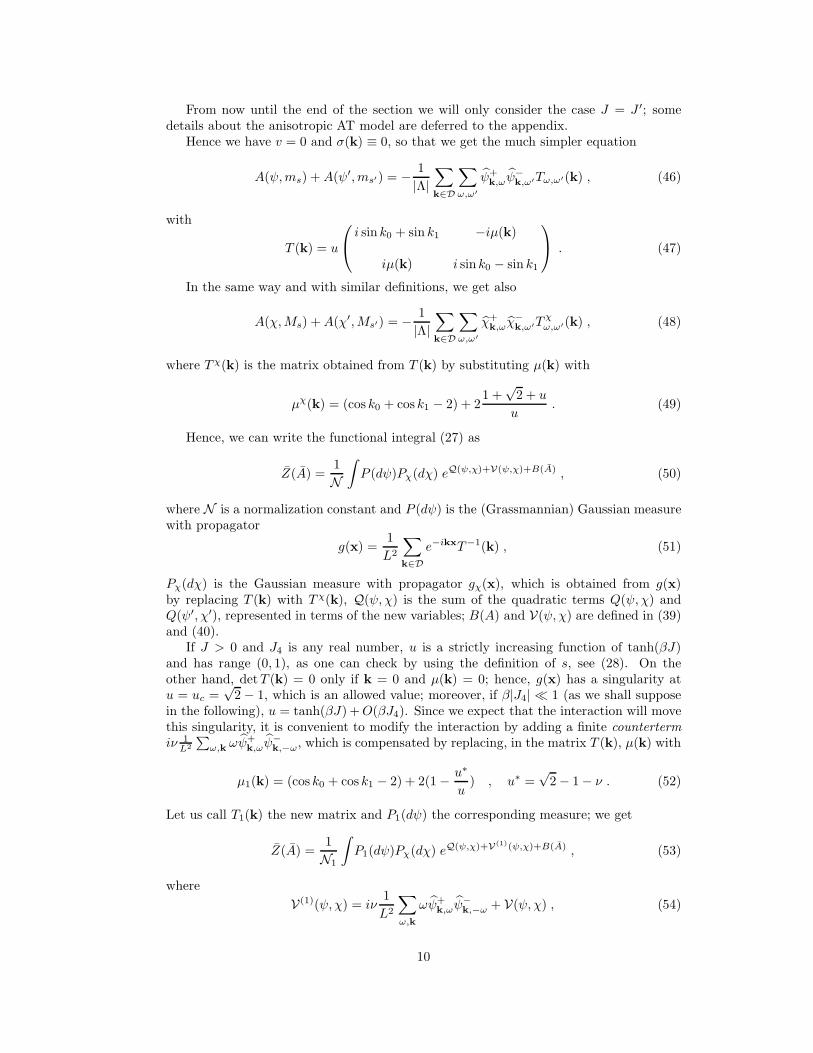
We need to improve the bound (89) when 2 − n−m ≥ 0. We can write, by using theproperties of the fermionic truncated expectations and the fact that, by the oddness of

the free propagator, W(1;0)ω (k) = 0,

W (0;2)(k)ω (x,y) = (90)

= λ∞

∫dwdw′ vK(x − w)g[k+1,N ]

ω (x − w′)W (1;2)(k)−ω;ω (w;w′,y) ,

which can be bounded, by using (89), as

ω ωx y = ω ω

x

w′

w

y

Figure 2: : Graphical representation of (90)

‖W (0;2)(k)ω ‖ ≤ |λ∞|‖vK‖L∞‖W (1;2)(k)

−ω;ω ‖N∑

j=k+1

‖g(j)ω ‖L1 ≤

≤ c11 − γ−1

γ2KC|λ∞|γ−k ≤ C1|λ∞|γkγ−2(k−K) , (91)

where, for example, C1 = max{2, c11−γ−1C}; hence (86) is proved. Note that the condition

C1 ≥ 2 is introduced only because C1 is the same constant appearing in (89).

ωx

ωy

ω′z

− δω′,ωω

z = x = y= ω

xu

ωy

w ω′z(a)

+

ωx = y

w

ω′z (b)

+

ωx u

ωy

w

ω′z (c)

+ δω′,ω

x = zω

uω

y

(d)

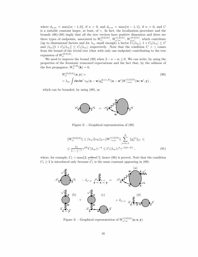
Figure 3: : Graphical representation of W(1;2)(k)ω′;ω (z;x,y)

16

Let us now consider W(1;2)(k)ω′;ω (z;x,y) and note that it can be decomposed as the sum

of the five terms in Fig.3, The term denoted by (a) in Fig.3 can be bounded as

‖W (1;2)(k)(a);ω′;ω‖ ≤ |λ∞|‖vK‖L∞‖W (2;2)(k)

ω′,−ω;ω‖N∑

j=k+1

‖g(j)ω ‖L1 ≤ CC1|λ∞|γ−2(k−K) . (92)

The bounds for the graphs (c) and (d) are an easy consequence of the the bound for

W(0;2)(k)ω .In order to obtain an improved bound also for the graph (b) of Fig. 3, we need to

further expand W(2;0)(k)ω,ω′ as done in Fig 4, if we suppose that the arrows in the fermion

lines of graph (b2) can be reversed.

ω

x w

u′

u

ω′

z

(b)

= δω′,−ωω

x w

−ωz

(b1)

+ω

x w

u′

z′u

w′

ω′

z

(b2)

+ω

x w u z′ω′

z

(b3)

Figure 4: : Graphical representation of graph (b) in Fig.3

The bound for the graph (b2) can be done by using the previous arguments. We canwrite

W(1;2)(k)(b2)ω′;ω(z;x,y) = λ2

∞δ(x − y)

∫dwdu′dz′ vK(x − w)vK(u′ − z′) ·

·∫dudw′ g[k+1,N ]

ω (w − u)g[k+1,N ]ω (u′ − w)g[k+1,N ]

ω (w′ − u′) ·

·W (2;2)(k)ω′,ω;−ω(z, z′;w′,u) . (93)

In order to get the right bound, it is convenient to decompose the three propagators gωinto scales and then bound by the L∞ norm the propagator of lowest scale, while the twoothers are used to control the integration over the inner space variables through their L1

norm. Hence we get:

‖W (1;2)(k)(b2)ω′;ω‖ ≤ |λ∞|2‖vK‖L∞‖vK‖L1‖W (2;2)(k)

ω′,−ω;ω‖ · (94)

·3!∑

k+1≤i′≤j≤i≤N‖g(j)ω ‖L1‖g(i)

ω ‖L1‖g(i′)ω ‖L∞ ≤ C3|λ∞|2γ−2(k−K) . (95)

for some constant C3.The bound of (b1) and (b3) requires a new argument, based on a cancelation following

from the particular form of the free propagator. Let us consider, for instance, (b1):

W(1;2)(k)(b1)ω′;ω(z;x,y) =

= λ∞δω′,−ωδ(x − y)

∫dw vK(x − w)

[g[k+1,N ]−ω (w − z)

]2. (96)

On the other hand, since the cutoff function Ck,N (k) is symmetric in the exchange between

k0 and k1, it is easy to see that g[k,N ]ω (x0, x1) = −iωg[k,N ]

ω (x1,−x0); hence∫du

[g[k+1,N ]−ω (u)

]2= 0 . (97)

17

It follows, by using (97) and the identity

vK(x − w) = vK(x − z) +∑

j=0,1

(zj − wj)

∫ 1

0

dτ(∂jvK

)(x − z + τ(z − w)

), (98)

that we can write

W(1;2)(k)(b1)ω′;ω(z;x,y) = λ∞δω′,−ωδ(x − y) · (99)

·∑

j=0,1

∫ 1

0

dτ

∫dw

(∂jvK

)(x − z + τ(z − w)

)(zj − wj)

[g[k+1,N ]−ω (w − z)

]2.

Hence,

‖W (1;2)(k)(b1)ω′;ω‖ ≤ 4|λ∞|

N∑

i=k

i∑

j=k

‖g(j)−ω‖L∞

∫dx∣∣(∂jvK)(x)

∣∣ · (100)

·∫dw |wj ||g(i)

−ω(w)| ≤ C4|λ∞|γ−(k−K) . (101)

By summing all the bounds, we see that there is a constant C2 such that

‖W (1;2)(k)ω′;ω − δω,ω′δ2‖ ≤ C2|λ∞|γ−(k−K) , (102)

which proves (87). The bound (88) for W (0;4)(k) follows from similar arguments.

3.3 Equivalence of the spin and the QFT models

As a consequence of the integration of the ultraviolet scales discussed in the previoussection, we can write the removed cutoffs limit of (82), with ϕ = J = 0 and with thechoice K = 0, as

liml→−∞

limN→∞

∫Pµ0,Z0(dψ

(≤0))eV(0)(ψ(≤0))+B(0)(ψ(≤0),A) , (103)

where the propagator of the integration measure in (103) coincides with g(≤0)T (x,y), de-

fined in (70), LV(0) = λ0F(0)λ and LB(0) is defined as in (67); from the analysis of the

previous section it follows that λ0 is a smooth function of λ∞, such that λ0 = λ∞+O(λ2∞).

The multiscale integration for the negative scales can be done exactly as described in§2.4, with the only difference that, by the oddness of the free propagator, νj = 0 and

λj−1 = λj + β(j)λ (λj , ...λ0) , (104)

where, by (69) and the short memory property,

β(j)λ (λj , ...λ0) = β

(j)λ (λj , ...λ0) +O(λ2

jγϑj) , (105)

β(j)λ (λj , ...λj) being the function appearing in the bound (74), so that we can prove in the

usual way that λ−∞ = λ0 +O(λ20); since λ0 = λ∞ +O(λ2

∞), we have

λ−∞ = h(λ∞) = λ∞ +O(λ2∞) , (106)

for some analytic function h(λ∞), invertible for λ∞ small enough. Moreover

Z±j−1

Z±j

= 1 + β(j)± (λj , ..., λ0) , (107)

18

withβ

(j)± (λj , ..., λ0) = β

(j)± (λj , ...λ0) +O(λ2

jγϑj) , (108)

β(j)± being the functions appearing in the analogous equations for the model of §2.4. This

implies that

η± = logγ [1 + β(−∞)± (λ−∞, ...λ−∞)] , (109)

that is the critical indices in the AT or 8V or in the model (82) are the same as functionsof λ−∞.

Of course λ−∞ is a rather complex function of all the details of the models. However,if we call λ′j(λ) the effective couplings of the lattice model of the previous sections, theinvertibility of h(λ∞) implies that we can choose λ∞ so that

h(λ∞) = λ′−∞(λ) . (110)

With this choice of λ∞(λ), the critical indices are the same, as they depend only on λ−∞;the rest of this chapter is devoted to the proof that the critical indices have, as functionsof λ∞, simple expressions, which imply the scaling relations in the main theorem.

Remark (109) and (110) play a central role in our analysis; they say that the criticalindices of the spin lattice models (1.1) are equal to the ones of the QFT model (82),provided that its coupling is chosen properly; such a model is defined in the continuumbut the non locality of the interaction has the effect that no ultraviolet divergences aregenerated. On the other hand, the model (82) verifies extra symmetries, involving WardIdentities and closed equation, which allow us to derive simple expressions for the indicesin terms of λ∞, as we will see in the following sections.

3.4 Ward Identities

We consider the case µ = 0 and we call Dω(k) = −ik0 + ωk. We shorten the notation ofWN (0, J, η) into WN (J, η). By the change of variables ψ±

x,ω → e±iαx,ωψ±x,ω we obtain the

identity

Dω(p)∂WN

∂Jp,ω

(0, η) − ν vK(p)D−ω(p)∂WN

∂Jp,−ω(0, η) = (111)

=

∫dk

(2π)2

[η+k+p,ω

∂WN

∂η+k,ω

(0, η) − ∂WN

∂η−k+p,ω

(0, η)η−k,ω

]+∂WA∂αp,ω

(0, 0, η) ,

where ν is a constant to be chosen later,

eWA(J,α,η) =

∫P (dψ[l,N ])eV

(N)(ψ[l,N ])+∑

ω

∫dx Jx,ωψ

[l,N ]+x,ω ψ

[l,N ]−x,ω

·e∑

ω

∫dx[ψ

[l,N ]+x,ω η−

x,ω+η+x,ωψ

[l,N ]−x,ω ]e[A0−νA−](α,ψ[l,N ]) ,

A0(α, ψ)def=∑

ω=±

∫dq dp

(2π)4Cω(q,p)αq−p,ωψ

+q,ωψ

−p,ω , (112)

A−(α, ψ)def=∑

ω=±

∫dq dp

(2π)4D−ω(p− q)vK(p − q)αq−p,ωψ

+q,−ωψ

−p,−ω , (113)

Cω(q,p) = [χ−1l,N (p) − 1]Dω(p) − [χ−1

l,N (q) − 1]Dω(q) , (114)

19

and χl,N (k) =∑N

k=l fk(k).

Remark - As explained in §2.2 of [8], (111) is obtained by introducing a cut-off functionχεl,N (k) never vanishing for all values of k 6= 0 and equivalent to χl,N (k) as far as the scal-ing properties of the theory are concerned; ε is a small parameter and limε→0+ χεl,N (k) =χl,N (k). This further regularization (to be removed before taking the removed cutoffslimit) ensures that the identity [(χεl,N )−1(k) − 1]χεl,N (k) = 1 − χεl,N (k) is satisfied for allk 6= 0. When this further regularization is removed, all the quantities we shall study havea well defined expression.

The two equations obtained from (111) by putting ω = ±1 can be solved w.r.t. ∂eWN/∂Jp,ω

and, if we define

a(p) =1

1 − ν vK(p), a(p) =

1

1 + ν vK(p),

Aε(p) =a(p) + εa(p)

2, (115)

we obtain the identity

∂eWN

∂Jp,ω

(0, η) −∑

ω′

Aωω′(p)

Dω(p)

∂eWA

∂αp,ω′

(0, 0, η) = (116)

=∑

ω′

Aωω′(p)

Dω(p)

∫dk

(2π)2

[η+k+p,ω′

∂eWN

∂η+k,ω′

(0, η) − ∂eWN

∂η−k+p,ω′

(0, η)η−k,ω′

].

Given a correlation function with m external fields of momenta k1, . . . ,km, we shallsay that its external momenta are non exceptional, if, for any subset I of {1, . . . ,m},∑

i∈I σiki 6= 0, where σi = +1 for the incoming momenta and σi = −1 for the outcomingmomenta. Note that our definitions are such that η+ is an incoming field, while η−, Jand α are outcoming.

An important role in this paper will have the following lemma, which was alreadyproved in [19].

Lemma 3.2 If λ∞ is small enough, there exists a choice of ν, independent of l and N ,such that

ν =λ∞4π

(117)

and, in the limit of removed cut-offs,

∑

ω′

Aωω′(p)

Dω(p)

∂eWA

∂αp,ω′

(0, 0, η) = 0 , (118)

in the sense that the correlation functions generated by deriving w.r.t. η the l.h.s. of (118)vanish in the limit of removed cutoffs, if the external momenta are non exceptional.

Proof. We sketch here the proof, as it will be useful in the following, referring for moredetails to [19] (see also [10] and [5, 9]). The starting point is the remark that WA(α, 0, η)is very similar to WN (J, η), see (82), the difference being that

∫Jx,ωψ

+x,ωψ

−x,ω is replaced

by A0−νA−. A crucial role in the analysis is played by the function Cω(p,q) appearing in

20

the definition of A0; this function is very singular, but it appears in the various equationsrelating the correlation functions only through the regular function

U (i,j)ω (q + p,q)

def= χN (p)Cω(q + p,q)g(i)

ω (q + p)g(j)ω (q) , (119)

where χN (p) is a smooth function, with support in the set {|p| ≤ 3γN+1} and equal to 1 in

the set {|p| ≤ 2γN+1}; we can add freely this factor in the definition, since U(i,j)ω (q+p,q)

will only be used for values of p such that χN (p) = 1, thanks to the support properties of

the propagator. It is easy to see that U(i,j)ω vanishes if neither j nor i equals N or l; this

has the effect that at least one of the fields in A0 has to be integrated at the N or l scale.As a matter of fact, the terms in which at least one field is integrated at scale l are much

easier to analyze, see below. In order to study the others, it is convenient to introduce

the function S(i,j)ω,ω defined by the equation

U (i,j)ω (q + p,q) =

∑

ω

Dω(p)S(i,j)ω,ω (q + p,q) . (120)

One can show that, if we define

S(i,j)ω,ω (z;x,y) =

∫dp dq

(2π)4e−ip(x−z)eiq(y−z)S

(i,j)ω,ω (p,q) , (121)

then, given any positive integer M , there exists a constant CM such that, if j > l,

|S(N,j)ω,ω (z;x,y)| ≤ CM

γN

1 + [γN |x − z|]Mγj

1 + [γj |y − z|]M , (122)

a bound which is used to control the renormalization of the marginal terms containing avertex of type A0. We choose ν as given by

ν = λ∞

N∑

i,j=l+1

∫dq

(2π)2S

(i,j)−ω,ω(q,q) ; (123)

by an explicit calculation one can see that, for any l < 0 and N > 0, ν satisfies (117). Weremark that, to get this result, it is important to exclude from the sum in the r.h.s. of(123) the couples (i, j) with one of the indices equal to l; without this restriction, ν wouldbe equal to 0, for any N > 0.

The fact that the external momenta are non exceptional is important to avoid theinfrared singularities of the correlation functions. This condition on the momenta is takeninto account by using the fact that, in the tree expansion of the correlation functions,there are important constraints on the scale indices of the trees. This allows us to safelybound the Fourier transforms of the correlation functions by the sum over the L1 normsin the coordinate space of the contributions associated to the different trees; see [5], §3.1,for an example of this strategy. Moreover, the tree structure of the expansion allows us toexpress the L1 norm of the correlation functions in terms of the L1 norm of the effectivepotential on the different scales; hence, in the following, in order to study the effect onthe Fourier transform of the correlations of the ultraviolet region, we shall study the L1

norm of the kernels in the coordinate space.We will proceed as in the analysis of WN (J, η), integrating first the ultraviolet scales

N,N − 1, . . . , h + 1, h ≥ K, following a procedure very similar to the one described in§3.2, the main difference being that there appear in the effective potential new monomialsin the external field α and in ψ.

21

We consider first the terms contributing to WA(α, 0, η) in which at least one of thetwo fields in A0 or A− is contracted at scale N . The marginal terms such that only oneof these two fields is contracted are proportional to W (0;2)(k), so that one can use (86)to bound them. Hence, we shall consider in detail only the terms such that both fields

of A0 or A1 are contracted and we shall call K(n;2m)(k)∆;ω;ω′ the corresponding kernels of the

monomials with 2m ψ-fields and n α-fields. In the case n = 1, we decompose them asfollows:

K(1;2m)(k)∆;ω;ω′ (p;k) =

∑

σ

Dσω(p)W(1;2m)(k)∆;σ,ω;ω′ (p;k) , (124)

where p is the momentum flowing along the external α-field. As in §3.2, we have to

improve the dimensional bound of W(1;2)(k)∆;σ,ω;ω′. We can write the following identity, which

is represented the first line of Fig.5 in the case σ = −1:

W(1;2)(k)∆;σ,ω;ω′(z;x,y) =

N∑

i,j=k

∫dudw S(i,j)

σω,ω(z;u,w)W(0;4)(k)ω,ω′ (u,w,x,y) −

−ν δ−1,σ

∫dw vK(z − w)W

(1;2)(k)−ω;ω′ (w;x,y) . (125)

ω

zu

w

ω′x

ω′y

− νN−ω

z w ω′x

ω′y

=ω

z u wω′

x

ω′y

(a)

− νN−ω

z = u w ω′x

ω′y

(b)

+ω

z

uu′

ww′

ω′y

ω′x

(c)

+ δω,ω′

ω

z

wω′

x

w′

ω′u = y(d)

− δω,ω′

ω

z

wω′

x

w′

u u′ω′y(e)

Figure 5: : Graphical representation of W(1;2)(k)∆;−1,ω;ω′

We can further decompose W(1;2)(k)∆;−1,ω;ω′ as in the last there lines of Fig.5. The term (c)

can be written as

λ∞

N∑

i,j=k

∫dudu′dwdw′ S(i,j)

−ω,ω(z;u,w)g[k,N ]ω (u − u′)vK(u − w′) ·

·W (1;4)(k)−ω;ω,ω′(w

′;u′,w,x,y) . (126)

22

Hence, if we put bj(x)def= γj/(1 + [γj |x|]3), we recall that S

(i,j)−ω,ω is different from 0 only

if either i or j is equal to N , and we use the bound (122), we see that the norm of (c) isbounded by

C3|λ∞|‖vK‖L∞

N ∗∑

i,j,m=k

∫dxdu′dwdw′ |W (1;4)(k)

−ω;ω,ω′(w′;u′,w,x,y)| ·

·∫dzdu bi(z − w)bj(z − u)|g(m)

ω (u − u′)| , (127)

where ∗ reminds that max{i, j} = N . Since the L1 and the L∞ norm of bj satisfy a bound

similar to analogous bounds of g(j)ω , we can proceed as in the previous section to bound∫

dzdu bi(z − w)bj(z − u)|g(m)ω (u − u′)|, by taking the L∞ norm for the factor with the

smaller index and the L1 norm for the other two. By also using (89), we get the bound

Cϑ|λ∞|2γ−2(k−K)γ−ϑ(N−k) , (128)

for any 0 < ϑ < 1 (Cϑ is divergent for ϑ → 1). With respect to analogous bound in§3.2 ((b2) in Fig.4), there is an improvement of a factor γ−ϑ(N−k). The term (d) can bebounded by

C|λ∞|‖vK‖L∞

N ∗∑

i,j=k

‖bi‖L1 ‖bj‖L1 ≤ C|λ∞|γ−(k−K)γ−(N−k) ;

for the term (e) we get the bound C|λ∞|2γ−3(k−K)γ−(N−k). By putting together all theprevious bounds, we get

‖(c) + (d) + (e)‖ ≤ Cϑ|λ∞|γ−(k−K)γ−ϑ(N−k) . (129)

We consider now the terms (a) and (b), whose sum can be written as

∫du

λ∞

N∑

i,j=k

S(i,j)−ω,ω(z;u,u) − νδ(z − u)

·

·∫dw vK(u − w)W

(1;2)(k)−ω;ω′ (w;x,y) . (130)

By using the identity (98), (130) can be written also as

λ∞N∑

i,j=k

∫du S

(i,j)−ω,ω(z;u,u) − ν

∫dw vK(z − w)W

(1;2),(k)−ω;ω′ (w;x,y) +

+λ∞∑

p=0,1

N∑

i,j=k

∫du S

(i,j)−ω,ω(z;u,u)(up − zp) · (131)

·∫ 1

0

dτ

∫dw (∂pvK)(z − w + τ(u − z))W

(1;2),(k)−ω;ω′ (w;x,y) .

The latter term is again irrelevant and vanishing for N − k → +∞; in fact, its norm canbe bounded by

2|λ∞|‖W (1;2),(k)−ω;ω′ ‖ ‖∂vK‖L1

N ∗∑

i,j=k

∫dz bi(z − u)bj(z − u)|u − zp| ≤

≤ C|λ∞|γ−(k−K)γ−(N−k) . (132)

23

Contrary to what happened for the graph (b1) of Fig4, the contribution of the graph (a)to the first term in the r.h. side of (131) is not zero (that is, the fermionic bubble is notvanishing); however, in this case its value is compensated by the graph (b), thanks to theexplicit choice we made for ν. Indeed we have

λ∞

N∑

i,j=k

∫du S

(i,j)−ω,ω(z;u,u) − ν = −2λ∞

k−1∑

j=l+1

∫du S

(N,j)−ω,ω(z;u,u) , (133)

that easily implies that the first term in the r.h. side of (131) is bounded by C|λ∞|γ−(N−k).

Let us finally consider W(1;2)(k)∆;+1,ω;ω′ , for which we can use a graph expansion similar to

that of Fig.5, the only differences being that ν is replaced by 0 and the indices −ω arereplaced by ω. Hence a bound can be obtained with the same arguments used above,with only one important difference: the contribution that in the previous analysis wascompensated by the graph (b) now is zero by symmetry reasons. Indeed, if we call k∗

the vector k rotated by π/2, it is easy to see that S(i,j)ω,ω (k∗,p∗) = −ωωS(i,j)

ω,ω (k,p), whichimplies that

N∑

i,j=k

∫du S(i,j)

ω,ω (z;u,u) =

N∑

i,j=k

∫dk

(2π)2S(i,j)ω,ω (k,−k) = 0 . (134)

We have then proved that

‖W (1;2)(k)∆;σ,ω;ω′‖ ≤ C|λ∞|γ−ϑ(N−k) , (135)

which implies, by dimensional bounds and the short memory property, that, for K ≤ k ≤N ,

‖W (1;2m)(k)∆;σ,ω;ω′ ‖ ≤ (C|λ∞|)mγ(1−m)kγ−ϑ(N−k) . (136)

It remains to analyze the terms contributing to WA(α, 0, η) in which no one of the twofields in A0 is contracted at scale N . If i ≥ l we can use the bound

∣∣∣∣∣U

(i,l)ω′ (q + p,q)

Dω(p)

∣∣∣∣∣ ≤ Cγ−(i−l) γ−l−i

Zi−1, if |p| ≥ 2γl+1 , (137)

and the factor γ−(i−l) in the r.h.s. of this bound is an improvement w.r.t. the dimensionalbound and makes indeed irrelevant the marginal terms containing a vertex of type A0, ifone of the ψ fields is contracted on scale l and p has a fixed value different from 0, as weare supposing.

The contributions to the correlation functions generated by the l.h.s. of (118), suchthat one of the ψ-fields in A0 is contracted at scale l (hence it is an external field at scalek), vanish in the limit l → −∞, if the momentum p of the α field is fixed at a valuedifferent from 0, as we are supposing. This follows from the bound (137), since the valueof i is essentially fixed at a value of order logγ |p| and the extra factor γ−(i−l) vanishes for

l → −∞. The correlations generated by the terms containing W(1;2m)(k)∆ are vanishing in

the limit of removed cut-offs, thanks to the extra factor γ−ϑ(N−k) in (136), with respectto the dimensional one, and the short memory property.

3.5 Closed equations

The Schwinger-Dyson equations for µ = 0 are generated by the identity, see [6],

Dω(k)∂eWN

∂η+k,ω

(0, η) = χl,N (k)

[η−k,ωe

WN (0,η) −

24

−λ∞∫

dp

(2π)2vK(p)

∂2eWN

∂Jp,−ω∂η+k+p,ω

(0, η)

]. (138)

By using (116) we easily get:

Dω(k)∂eWN

∂η+k,ω

(0, η) = χl,N (k)

{η−k,ωe

WN (0,η) −

−λ∞∑

ω′

∫dp

(2π)2vK(p)

A−ωω′(p)

D−ω(p)· (139)

·∫

dq

(2π)2

[η+q+p,ω′

∂eWN

∂η+q,ω′∂η

+k+p,ω

(0, η) − ∂eWN

∂η+k+p,ω∂η

−q+p,ω′

(0, η)η−q,ω′

]−

−λ∞∑

ω′

∫dp

(2π)2vK(p)

A−ωω′(p)

D−ω(p)

∂2eWA

∂αp,ω′∂η+k+p,ω

(0, 0, η)

}.

We now want to prove that the last term in the r.h.s. of (139) is negligible in the limit ofremoved cutoffs, if k is fixed at a value far from the cutoffs.

Theorem 3.3 In the limit of removed cutoffs, the correlation functions generated by de-riving w.r.t. η the functional

∑

ω′

∫dp

(2π)2vK(p)

A−ωω′(p)

D−ω(p)

∂2eWA(0,0,η)

∂αp,ω′∂η+k+p,ω

(140)

vanish, if the external momenta are non exceptional.

Proof. It is convenient to write (140) as∑

ε=±∂WT,ε

∂βk,ω

(0, η), where

eWT,ε(β,η) =

∫P (dψ[l,N ])eV

(N)(ψ[l,N ])+∑

ω

∫dx[ψ

[l,N ]+x,ω η−

x,ω+η+x,ωψ

[l,N ]−x,ω ] ·

· e

[T

(ε)1 −νT (ε)

−

](ψl,N ,β) (141)

and

T(ε)1 (ψ, β) =

∑

ω

∫dk dp dq

(2π)4v(ε)K (p)

C−εω(q + p,q)

D−ω(p)·

· βk,ωψ−k+p,ωψ

+q+p,−εωψ

−q,−εω , (142)

T(ε)− (ψ, β) =

∑

ω

∫dk dp dq

(2π)4u

(ε)K (p)βk,ωψ

−k+p,ωψ

+q+p,εωψ

−q,εω , (143)

where

v(ε)K (p)

def= vK(p)Aε(p) , u

(ε)K (p) = v

(ε)K (p)vK(p)

Dεω(p)

D−ω(p). (144)

Note that v(±)K (x) and u

(−)K (x) are smooth functions of fast decay, hence they are equivalent

to vK(x) in the bounds. This is not true for u(+)K (x), whose Fourier transform is bounded

but discontinuous in p = 0. However, in the following we shall only need to know that

‖u(+)K ‖L∞ ≤ Cγ2K and that |u(+)

K (p)| ≤ |v(+)K (p)vK(p)|, which are easy to prove.

As in §3.4, we now perform a multiscale integration for the ultraviolet scales N,N −1, . . . , k + 1, k ≥ K, very similar to the one described in §3.2, the main difference being

25

that that there appear in the effective potential new monomials in the external field β andin ψ. As explained in the previous section, in order to control the Fourier transform atnon exceptional momenta of the correlation functions, it is in general sufficient to control,in the ultraviolet region, the L1 norm in coordinate space of the kernels appearing in theeffective potential. This is in general true also in the proof of this theorem, except for abound, where one has to be more careful, see below.

The contributions to the correlation functions such that one of the ψ-fields in T(ε)1 (ψ, β)

with momentum q + p or q, see (142), is contracted at scale l (hence it is an externalfield at scale k), vanish in the limit l → −∞, if the momentum k of β is fixed at a valuedifferent from 0, as we are supposing. In fact, in this case either |p| or |k + p| is greaterthan |k|/2; hence, by using (137) or the short memory property, these contributions satisfya bound containing the extra factor γl|k/2|, which vanishes for l → −∞. We considerthen just the terms contributing to WT,ε(β, η), in which at least one of the two ψ-fields in

T(ε)1 (ψ, β) with momentum q + p or q is contracted at scale N . We shall call W

(1;2m−1)T,ε;ω;ω′

the corresponding kernels of the monomials with 2m− 1 ψ-fields and 1 α-field. We claimthat

‖W (1;2m−1)(k)T,ε;ω;ω′ ‖ ≤ Cγ(2−m)kγ−ϑ(N−k) . (145)

By the usual arguments, this is a consequence of the improved bounds:

‖W (1;1)(k)T,ε;ω,ω ‖ ≤ C|λ∞|γkγ−ϑ(N−k)γ−2(k−K) , (146)

‖W (1;3)(k)T,ε;ω,ω′‖ ≤ C|λ∞|γ−ϑ(N−k) . (147)

We prove first the bound (146). We can write

W(1;1)(k)T,ε;ω,ω = W

(1;1)(k)(a)T,ε;ω,ω +W

(1;1)(k)(b)T,ε;ω,ω (148)

wherea) W

(1;1)(k)(a)T,ε;ω,ω is the sum over the terms such that the field β belongs only to a T

(ε)1 -

vertex, whose ψ-field ψ+q+p,−εω either is contracted with ψ−

k+p,ω (this can happen only for

ε = −1) or is connected to it through a kernel W(0;2)(k)ω (q + p).

b) W(1;1)(k)(b)T,ε;ω,ω is the sum over the remaining terms.

Let us consider the first term. Given k, for N large enough, χ−1l,N (k) − 1 = 0; hence

we can write:

W(1;1)(k)(a)T,ε;ω,ω(k) = δε,−1

∫dp

(2π)2v(−1)K (p)

D−ω(p)[χ−∞,N (p + k) − 1] · (149)

·[1 + g[k+1,N ]

ω (p + k)W (0;2)(k)ω (p + k)

] [1 + g[k+1,N ]

ω (k)W (0;2)(k)ω (k)

].

Moreover, since v(−1)K (p) = 0 for |p| ≥ 2γK , then χ−∞,N (p + k) − 1 = 0, if v

(−1)K (p) 6= 0

and N is large enough. It follows that, given a fixed k, for N large enough,

W(1;1)(k)(a)T,ε;ω,ω(k) = 0 . (150)

Let us now consider W(1;1)(k)(b)T,ε;ω,ω(x − y), which can be decomposed as in Fig. 6.

By using (125), it can be written as

∑

σ

∫dz u

(ε)K (x − z)g[k,N ]

ω (x − w)W(1;2)(k)∆;σ,−εω;ω(z;y,w) , (151)

26

ωx

ωy

z

w

− ν ωx

z

ωyy

w

Figure 6: : Graphical representation of W(1;1)(k)(b)T,ε;ω,ω

hence its norm, by using (135), can be bounded by

‖u(ε)K ‖L∞

N∑

j=k

|g(j)ω |L1‖W (1;2)(k)

∆;σ,−εω;ω‖ ≤ C|λ∞|γkγ−2(k−K)γ−ϑ(N−k) . (152)

In order to prove the bound (147), we write

W(1;3)(k)T,ε;ω;ω′ = W

(1;3)(k)(a)T,ε;ω;ω′ +W

(1;3)(k)(b)T,ε;ω;ω′ , (153)

where W(1;3)(k)(a)T,ε;ω;ω′ contains the terms in which the field ψk+p,ω of T1 and T− is not con-

tracted or is linked to a kernel W(0;2)(k)ω , while the other terms are collected in W

(1;3)(k)(b)T,ε;ω;ω′ .

Let us consider first W(1;3)(k)(a)T,ε;ω;ω′ ; its Fourier transform, if we call k+ and k− the momenta

of the two fields connected to the line u(ε)K , can be written as (note that ω′ is of the form

(ω, ω′, ω′)):

W(1;3)(k)(a)T,ε;ω;ω′(k;k+,k−) =

[1 + g[k+1,N ]

ω (k + k+ − k−)W (0;2)(k)ω (k + k+ − k−)

]·

·u(ε)K (k+ − k−)

∑

σ

W(1;2)(k)∆;σ,−εω,ω′(k

− + k+ − k−,k−) . (154)

Then, if ε = −1, since ‖v(−1)K ‖L1 ≤ C, by using the bounds (135) and (86), we find

‖W (1;3)(k)(a)T,−1;ω;ω′‖ ≤ C|λ∞|γ−ϑ(N−k) (155)

This bound is not true in the case ε = +1, where it is necessary to take carefully intoaccount that we are indeed bounding the Fourier transform of the correlation functionsgenerated by (140), at fixed (non exceptional) external momenta.

The terms contributing to these correlations and containing W(1;3)(k)(a)T,+1;ω;ω′ as a cluster

can be of two different types. There are terms such that the line corresponding to ψk+p,ω

is connected to the rest of the graph only through the vertex of the field β. In this case,we have to bound an expression of the type

u(+1)K (k − q)G1(k

′)G2(k′′) , (156)

where k′ and k′′ are a set of independent external momenta, q = −∑i σik′i, q − k =∑

i σik′′i and G2(k

′′) contains the cluster associate to∑

σ W(1;2)(k)∆;σ,−ω,ω′ ; this expression is

bounded by C‖G1‖ |Γ2‖, the same result that we should get in the case ε = −1, bybounding the full expression with the ‖ · ‖ norm. Hence, the final bound is the same wewould obtain by using (155) for ε = +1.

We still have to consider the terms such that the line corresponding to ψk+p,ω isconnected to the rest of the graph even if we erase the vertex of the field β. Now we have

27

to bound an expression of the type∫

dp

(2π)2u

(+1)K (p)g(j)(p + k)G(p,k′) , (157)

where∑i σiki = k and G(p,k′) contains the cluster associate to

∑σ W

(1;2)(k)∆;σ,−ω,ω′ ; this

expression can be bounded by C‖g‖L1‖G‖, the same result that we should get in the caseε = −1, by bounding the full expression with the ‖ · ‖ norm.

Let us finally consider W(1;3)(k)(b)T,ε;ω;ω′ , which can be represented as in Fig.7.

(b1)

ωx

z

wω′

v

ω′

u

ω

y

(b2)

− νN ωx

z

wω′

v

ω′

u

ω

y

+

(b3)

ωx

z εω

w

ω′v

ω′u

+

(b4)

ωx

z εω

w

ω′v

ω′u

Figure 7: : Graphical representation of W(1;3)(k)(b)T,ε;ω;ω′

We can write

W(1;3)(k)(b)T,ε;ω,ω′(x,y,u,v) = (158)

=

∫dzdw u

(ε)K (x − z)g[k,N ]

ω (x − w)W(1;4)(k)∆,ε;ω,ω′(z;w,y,u,v) ,

so that, by the bounds (135), ‖W (1;4)(k)∆,ε;ω,ω′‖ ≤ C|λ∞|γ−kγ−ϑ(N−k) and ‖u(ε)

K ‖L∞ ≤ Cγ2K ,we get:

‖W (1;3)(k)(b)T,ε;ω;ω′‖ ≤ C|λ∞|γ−2(k−K)γ−ϑ(N−k) . (159)

Again, with respect to the analogous bound in §3.2,we have an extra factor γ−ϑ(N−k) andthis implies, proceeding for instance as in §4.1 of [5], the proof of the Theorem.

3.6 Solution of the closed equations and proof of x+x−

= 1

We want to solve the closed equations for the correlation functions

〈ψ−x,ωψ

+y,ω〉

def= Sω(x − y) , (160)

〈ψ−x,ωψ

−y,−ωψ

+u,−ωψ

+v,ω〉

def= Gω(x,y,u,v) , (161)

in the limit of removed cutoffs. By taking in (139) one derivative w.r.t. η−k,ω and thenputting η ≡ 0, we find

Dω(k)Sω(k) = 1 + λ∞

∫dp

(2π)2FK,−(p)Sω(k + p) , (162)

where

FK,ε(p)def=

vK(p)Aε(p)

D−ω(p). (163)

28

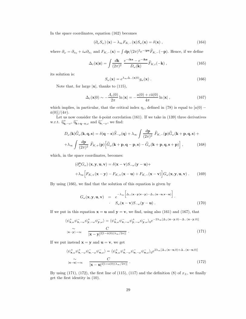
In the space coordinates, equation (162) becomes

(∂ωSω) (x) − λ∞FK,−(x)Sω(x) = δ(x) , (164)

where ∂ω = ∂x0 + iω∂x1 and FK,−(x) =∫dp/(2π)2e−ipxFK,−(−p). Hence, if we define

∆ε(x|z) =

∫dk

(2π)2e−ikx − e−ikz

Dω(k)FK,ε(−k) , (165)

its solution is:Sω(x) = eλ∞∆−(x|0)gω(x) . (166)

Note that, for large |x|, thanks to (115),

∆ε(x|0) ∼ −Aε(0)

2πln |x| = −a(0) + εa(0)

4πln |x| , (167)

which implies, in particular, that the critical index ηz, defined in (78) is equal to [a(0) −a(0)]/(4π).

Let us now consider the 4-point correlation (161). If we take in (139) three derivativesw.r.t. η+

q,−ω, η−k+q−s,ω and η−s,−ω, we find:

Dω(k)Gω(k,q, s) = δ(q − s)S−ω(q) + λ∞

∫dp

(2π)2FK,−(p)Gω(k + p,q, s) +

+λ∞

∫dp

(2π)2FK,+(p)

[Gω(k + p,q − p, s) − Gω(k + p,q, s + p)

], (168)

which, in the space coordinates, becomes:

(∂xωGω) (x,y,u,v) = δ(x − v)S−ω(y − u)+

+λ∞[FK,+(x − y) − FK,+(x − u) + FK,−(x − v)

]Gω(x,y,u,v) . (169)

By using (166), we find that the solution of this equation is given by

Gω(x,y,u,v) = e−λ∞

[∆+(x−y|v−y)−∆+(x−u,v−u)

]

·· Sω(x − v)S−ω(y − u) . (170)

If we put in this equation x = u and y = v, we find, using also (161) and (167), that

〈ψ+x,ωψ

−x,−ωψ

+y,−ωψ

−y,ω〉 = 〈ψ+

x,ωψ−x,−ωψ

+y,−ωψ

−y,ω〉0e−2λ∞[∆+(x−y,0)−∆−(x−y,0)]

∼|x−y|→∞

C

|x − y|2[1−a(0)(λ∞/2π)]. (171)

If we put instead x = y and u = v, we get

〈ψ+x,ωψ

+x,−ωψ

−u,−ωψ

−u,ω〉 = 〈ψ+

x,ωψ+x,−ωψ

−u,−ωψ

−u,ω〉0e2λ∞[∆+(x−u,0)+∆−(x−u,0)]

∼|x−u|→∞

C

|x − u|2[1+a(0)(λ∞/2π)]. (172)

By using (171), (172), the first line of (115), (117) and the definition (8) of x±, we finallyget the first identity in (10).

29

4 Appendix: the anisotropic Ashkin-Teller model

In this appendix, in order to derive (12), we briefly recall the analysis of the anisotropicAshkin-Teller model in [13]. The integration procedure is similar to that described in §2,the main difference being that the quadratic part (42) of the interaction now contains

also terms of the form ψε(≤h)x,ω ψ

ε(≤h)x,−ω . It follows, see (12) (where different definitions of the

fermion fields were used) for details, that we have to substitute the Grassmann integrationPZh,µh

(dψ(≤h)) in (64) with a new measure PZh,µh,σh(dψ(≤h)), where µh and σh are the

constants multiplying, respectively, the quadratic mass terms

2∑

ω=±ψ(≤h)+

x,ω ψ(≤h)−x,−ω and − 2i

∑

ε=±ψ

(≤h)εx,+ ψ

(≤h)εx,− . (173)

One can see that

| logγ(µj−1/µj) − ηµ(λ−∞)| ≤ Cλ2γϑj ,

| logγ(σj−1/σj) − ησ(λ−∞)| ≤ Cλ2γϑj . (174)

Hence, since the two mass terms are clearly proportional, respectively, to the operatorsO+ and O−, we find that

ηµ = η+ − ηz , ησ = η− − ηz . (175)

It turns out that the difference of the critical temperatures scales as |v|xT where xT , see(5.26) of [13] (where the indices are defined with a different sign and the definitions of µhand σh are exchanged), is given by

xT =1 + ηµ1 + ησ

, (176)

which implies (12), since ηµ = 1 − x+ and ησ = 1 − x−.

Acknowledgments P.F. is indebited with David Brydges for stimulating his interest inthe topic with the request of a review seminar on the papers [24] and [18].

References

[1] Ashkin J., Teller E.: Statistics of Two-Dimensional Lattices with Four Compo-nents. Phys. Rev. 64, 178 - 184, (1943).

[2] Baxter R.J.: Eight-Vertex Model in Lattice Statistics. Phys. Rev. Lett. 26, 832–833, (1971).

[3] Baxter R.J.: Exactly solved models in statistical mechanics. Academic Press, Inc.London, (1989).

[4] Barber M., Baxter R.J.: On the spontaneous order of the eight-vertex model. J.Phys. C 6, 2913–2921, (1973).

[5] Benfatto G., Falco P., Mastropietro V.: Functional Integral Construction of theMassive Thirring model: Verification of Axioms and Massless Limit. Comm.Math. Phys. 273, 67–118, (2007).

30

[6] Benfatto G., Falco P., Mastropietro V.: Massless Sine-Gordon and MassiveThirring Models: proof of the Coleman’s equivalence. Comm. Math. Phys., toappear (2008).

[7] Benfatto G., Mastropietro V.: Rev. Math. Phys. 13, 1323–1435, (2001).

[8] Benfatto G., Mastropietro V.: On the Density-Density Critical Indices in Inter-acting Fermi Systems. Comm. Math. Phys. 231, 97–134, (2002).

[9] Benfatto G., Mastropietro V.: Ward Identities and Chiral Anomaly in the Lut-tinger Liquid. Comm. Math. Phys. 258, 609–655, (2005).

[10] Falco P., Mastropietro V.: Renormalization Group and Asymtotic Spin–ChargeSeparation for Chiral Luttinger Liquid. J.Stat.Phys. 131, 79–116, (2008).

[11] Giuliani A., Mastropietro V.: Anomalous Critical Exponents in the AnisotropicAshkin-Teller Mode Phys. Rev. Lett. 93, 190603–07, (2004).

[12] Giuliani A., Mastropietro V.: Anomalous Universality in the AnisotropicAshkinaTeller Model. Comm. Math. Phys. 256, 681–725, (2005).

[13] Kadanoff L.P.: Connections between the Critical Behavior of the Planar Modeland That of the Eight-Vertex Model. Phys. Rev. Lett. 39, 903–905, (1977).

[14] Kadanoff L.P., Brown A.C.: Correlation functions on the critical lines of theBaxter and Ashkin-Teller models. Ann. Phys. 121, 318–345, (1979).

[15] Kadanoff L.P., Wegner F.J.: Some Critical Properties of the Eight-Vertex Model.Phys. Rev. B 4, 3989–3993, (1971).

[16] Luther A., Peschel I.: Calculations of critical exponents in two dimension fromquantum field theory in one dimension. Phys. Rev. B 12, 3908–3917, (1975).

[17] Mastropietro V.: Non-Universality in Ising Models with Four Spin Interaction.J. Stat. Phys. 111, 201–259, (2003).

[18] Mastropietro V.: Ising Models with Four Spin Interaction at Criticality. Comm.Math. Phys. 244 595–64 (2004).

[19] Mastropietro V.: Nonperturbative Adler-Bardeen theorem. J. Math. Phys 48,022302, (2007).

[20] Mastropietro V.: Non-perturbative aspects of chiral anomalies. J. Phys. A 40,10349–10365, (2007).

[21] Mastropietro V.: Non-perturbative Renormalization. World Scientific, (2008).

[22] den Nijs M.P.M.: Derivation of extended scaling relations between critical ex-ponents in two dimensional models from the one dimensional Luttinger model.Phys. Rev. B 23, 6111–6125, (1981).

[23] Pruisken A.M.M. Brown A.C.: Universality for the critical lines of the eightvertex, Ashkin-Teller and Gaussian models. Phys. Rev. B 23, 1459–1468, (1981).

[24] Pinson H., Spencer T.: Unpublished.

[25] Samuel S. The use of anticommuting variable integrals in statistical mechanics.I. The computation of partition functions. J. Math. Phys. 21, 2806, (1980).

31

[26] Smirnov S.: Towards conformal invariance of 2D lattice models. ProceedingsMadrid ICM, Europ. Math. Soc, 2006 - arXiv:0708.0032

[27] Spencer T. A mathematical approach to universality in two dimensions. PhysicaA 279, 250–259, (2000).

[28] Zamolodchikov A.B., Zamolodchikov Al. B.: Conformal field theory and 2D crit-ical phenomena, part 1. Soviet Scientific Reviews A 10, 269, (1989).

32