Dynamic user equilibrium based on a hydrodynamic model

Dynamic user equilibrium based on a hydrodynamic modelq

Terry L. Friesz a,!, Ke Han b, Pedro A. Neto a, Amir Meimand a, Tao Yao a

aDepartment of Industrial and Manufacturing Engineering, Pennsylvania State University, PA 16802, USAbDepartment of Mathematics, Pennsylvania State University, PA 16802, USA

a r t i c l e i n f o

Keywords:LWR modelDynamic user equilibriumDynamic network loadingLax–Hopf formula

a b s t r a c t

In this paper we present a continuous-time network loading procedure based on the Light-hill–Whitham–Richards model proposed by Lighthill and Whitham (1955) and Richards(1956). A system of differential algebraic equations (DAEs) is proposed for describing trafficflow propagation, travel delay and route choices. We employ a novel numerical apparatusto reformulate the scalar conservation law as a flow-based partial differential equation(PDE), which is then solved semi-analytically with the Lax–Hopf formula. This approachallows for an efficient computational scheme for large-scale networks. We embed this net-work loading procedure into the dynamic user equilibrium (DUE) model proposed by Frieszet al. (1993). The DUE model is solved as a differential variational inequality (DVI) using afixed-point algorithm. Several numerical examples of DUE on networks of varying sizesare presented, including the Sioux Falls network with a significant number of paths andorigin–destination pairs (OD).The DUE model presented in this article can be formulated as a variational inequality (VI)

as reported in Friesz et al. (1993). We will present the Kuhn–Tucker (KT) conditions for thatVI, which is a linear system for any given feasible solution, and use them to check whethera DUE solution has been attained. In order to solve for the KT multiplier we present adecomposition of the linear system that allows efficient computation of the dual variables.The numerical solutions of DUE obtained from fixed-point iterations will be tested againstthe KT conditions and validated as legitimate solutions.

! 2012 Elsevier Ltd. All rights reserved.

1. Introduction

Dynamic traffic assignment (DTA) models determine departure rates, departure times and route choices over a givenplanning horizon. They seek to describe the dynamic evolution of traffic in networks in a fashion consistent with the funda-mental notions of traffic flow and travel demand. This paper is concerned with a specific type of dynamic traffic assignmentknown as dynamic user equilibrium (DUE) for which generalized travel cost is identical for route and departure time choicesassociated with any given origin–destination (OD) pair.

1.1. Dynamic user equilibrium (DUE): a brief review

DUE is the primary form of DTA that this paper will focus on. The last two decades have seen many efforts to develop atheoretically sound formulation of dynamic network user equilibrium that is also in a canonical form acceptable to scholarsand practitioners alike. DUE models tend to be comprised of four essential subproblems:

0191-2615/$ - see front matter ! 2012 Elsevier Ltd. All rights reserved.http://dx.doi.org/10.1016/j.trb.2012.10.001

q This work is partially supported by NSF through grant EFRI-1024707, ‘‘A theory of complex transportation network design’’, and by an NSF GraduateResearch Fellowship under Grant no. DGE-0750756.! Corresponding author. Tel.: +1 814 863 2445.

E-mail addresses: [email protected] (T.L. Friesz), [email protected] (K. Han), [email protected] (P.A. Neto), [email protected] (A. Meimand),[email protected] (T. Yao).

Transportation Research Part B 47 (2013) 102–126

Contents lists available at SciVerse ScienceDirect

Transportation Research Part B

journal homepage: www.elsevier .com/ locate / t rb

http://dx.doi.org/10.1016/j.trb.2012.10.001

mailto:[email protected]





http://dx.doi.org/10.1016/j.trb.2012.10.001

http://www.sciencedirect.com/science/journal/01912615

http://www.elsevier.com/locate/trb

1. a model of path delay;2. flow dynamics;3. flow propagation constraints; and4. a route and departure-time choice model.

Furthermore, there are two major components of item 4 above: (a) the mathematical expression of Nash-like equilibriumconditions and (b) a network performance model which is an embedded dynamic network loading (DNL) problem. In theDNL procedure arc-specific volumes, arc-specific exit rates and experienced path delay are determined when departure ratesare known for each path, see Friesz et al. (2011). It is the embedded dynamic network loading (DNL) problem that makesDUE so difficult. An unfortunate and yet popular misconception is that devising a separate algorithm for the DNL problemmeans one has chosen a sequential approach to DUE, whereby one first solves the DNL problem then solves the DUE prob-lem, without requiring or attaining consistency. Such a perspective is not even remotely correct. Instead, the DNL processshould be understood as the embodiment of the state operator introduced in Friesz et al. (2011) and Friesz (2010) andnot as some sort of approximation.1

Some early analytical DUE models were greatly influenced by the dynamic system optimal models presented in Merchantand Nemhauser (1978a,b) as well as by a desire to find an equivalent optimization problem. In Friesz et al. (1989), and laterin Ran et al. (1993), a Beckmann-type objective function is employed to create an optimal control problem whose solutionsare of the DUE type. Friesz et al. (1993) showed a variational inequality may be used to represent dynamic user equilibriumwhen there are both route and departure time decisions. Following suit, Ran and Boyce (1996) suggested other variationalinequality (VI) formulations of DUE with somewhat unusual flow propagation constraints that are meant to avoid theimposition of state constraints while also assuring physically realistic flows; unfortunately their constraints do not reflectthe contraction and expansion of vehicle platoons and are intrinsically inconsistent with other aspects of their model aspointed out by Friesz et al. (2011). In contrast, Friesz et al. (2011) utilized flow propagation constraints that involved bothstate and control variables as well as state-dependent time shifts to account for expansion and contraction of platoons whilealso maintaining model consistency. A dual-time-scale formulation of DUE with demand evolution was also presented inFriesz et al. (2011) where a differential variational inequality (DVI) formulation was used to model dynamic user equilibrium.The authors implemented a fixed-point algorithm to solve the DVI. The DNL phase of DUE is expressed in Friesz et al. (2011)as a system of differential algebraic equations (DAEs) and approximated as a system of ordinary differential equations (ODEs).Moreover, Friesz et al. (2011) also showed the compatibility of the proposed DUE formulation with the CTM proposed inDaganzo (1994, 1995). The papers, Wu et al. (1998) and Xu et al. (1999) developed algorithms for the model introducedin Friesz et al. (1993) based upon the gradient projection method without any proof of convergence. The CTM was employedby Lo and Szeto (2002) to create link dynamics as well as a path travel time extraction procedure. Their procedure allows theCTM to subsume the role of the effective path delay operator as originally articulated by Friesz et al. (1993).

Zhu and Marcotte (2000) showed that when departure rates have uniform upper bounds, a solution exists for thecontinuous-time user equilibrium with route choices. Recently in Han et al. (2012a), the existence of a simultaneous route-and-departure choice DUE has been establishedwithout assuming a priori bounds on the path flows. In that paper, the authorsused the generalized Vickrey model developed in Han et al. (in press-a, in press-b) for the embedded DNL sub-problem.

1.2. Dynamic traffic flow models

An essential component of many DTA models is the DNL procedure, which determines traffic states from the link dynam-ics. The accurate and efficient computation of the DNL sub-problem is crucial to the overall performance of the DTA model.The primary purpose of the DNL procedure within the DUE model is to numerically evaluate the so-called effective delayoperator introduced by Friesz et al. (1993), which is not available in closed-form. The DNL procedure determines path-specific travel times given a set of known routing and departure time choices. The outcome of the DNL sub-problem reliesheavily on the type of link model and junction model chosen. In this section, we will review a few macroscopic traffic flowmodels most commonly used in the current literature, leading up to the Lighthill–Whitham–Richards (LWR) model of Light-hill and Whitham (1955) and Richards (1956) that we will consider in this paper.

1.2.1. Macroscopic link modelsWe start our discussion with single link loading. Depending on the ways of specifying flow propagation, we distinguish

between delay-function models and the exit-flow function models. The former is described and solved based on an explicittravel delay function given exogenous parameters that are typically estimated by fitting functions to real-world data. Oneexample is the link delay model (LDM); see Friesz et al. (1993), Wu et al. (1998) and Xu et al. (1999). In contrast, exit-flowfunction models are based on explicitly modeling the underlying flow dynamics as demonstrated by the M–N model of Mer-

1 Note that, by referring to the network loading procedure, we are neither employing nor suggesting a sequential approach to the study and computation ofDUE. Rather a subset of the equations and inequalities comprising a complete DUE model may be grouped in a way that identifies a traffic assignmentsubproblem and a network loading subproblem. Such a grouping and choice of names is merely a matter of convenient language that avoids repetitive referenceto the same mathematical expressions. Use of such language does not alter the need to solve both the assignment and loading problems consistently and, thus,simultaneously. A careful reading of the mathematical presentation made in subsequent sections makes this assertion quite clear.

T.L. Friesz et al. / Transportation Research Part B 47 (2013) 102–126 103

chant and Nemhauser (1978a,b), the cell transmission model (CTM) of Daganzo (1994, 1995) and Vickrey’s model (VM) ofVickrey (1969).

Among the link models mentioned above, the CTM is the most widely used model in the realm of DNL primarily because:(1) it is based on simple rules for the propagation of traffic states over discrete cells; (2) it is easy to extend to a network; and(3) it captures several key phenomena of real-world traffic such as shock waves and spillback. It has been shown in Daganzo(1994) that the CTM is the discrete version of LWR model on a single arc, given a trapezoidal density–flow relationship. Onelimitation of the CTM lies in the computational inefficiency as the algorithm stores and updates traffic quantities in a two-dimensional cell. In Nie and Zhang (2008), where a comparative study of various link models was conducted, the CTM wasshown to be computationally demanding in terms of solution time and memory consumption.

1.2.2. LWR network modelThe LWR model is another macroscopic link model that describes traffic dynamics in terms of the formation, propagation

and interaction of kinematic waves. It has received increased attention in the field of traffic flow theory in the past severaldecades due to its capability of capturing key features of vehicular traffic such as shock waves and spillback. The primarymathematical form of LWR model is a partial differential equation (PDE) describing the temporal–spatial evolution of averagedensity and flow. The PDE of interest here is based on conservation of vehicles and an explicit density–flow relation knownas the fundamental diagram

@

@tq!t; x" # @

@xf !q!t; x"" $ 0 !1:1"

where q(t,x) denotes the local vehicle density and f(q(t,x)) is the flow. The fundamental diagram f(%) is a continuous and con-cave function defined on [0,qjam] where qjam is the jam density. The fundamental diagram encodes the speed-density rela-tion and is calibrated using empirical data. Classical mathematical results on the first-order PDEs of the form (1.1) can befound in Bressan (2000). For a detailed discussion of numerical schemes for conservation laws, we refer the reader to Godu-nov (1959) and LeVeque (1992).

The extension of LWR model to networks has been studied extensively in the literature: a list of selected references in-clude Coclite et al. (2005), Daganzo (1994, 1995), Garavello and Piccoli (2006), Holden and Risebro (1995), Jin (2010), Jin andZhang (2003) Lebacque (1996) and Lebacque and Khoshyaran (1999). A detailed survey can also be found in Zhang (2001).

The primary difficulty with the LWR-based network loading problem stems from the complex boundary conditions at ajunction of arbitrary topology. Holden and Risebro (1995) were among the first to propose an analytical framework to derivethe weak entropy solution of conservation laws at the junction. In particular, they extended the notion of weak solution to asingle conservation law to several conservation laws with coupling boundary conditions. In order to isolate a unique solutionat the junction, an entropy condition was introduced which amounts to optimizing some abstract objective function. In Coc-lite et al. (2005), the notion of entropy condition was instantiated by maximizing the flux through the junction over all pos-sible boundary fluxes of links incident to the junction. They solved the Riemann problems at junctions with fixed vehicleturning percentages. However, these conditions are insufficient to isolate a unique solution in the case where the numberof incoming links exceeds that of outgoing links. To overcome this difficulty, the authors introduced a right-of-way parameterspecifying the priority of incoming vehicles.

Complex boundary conditions can be relatively easily analyzed using demand–supply functions proposed in Lebacque(1996) and Lebacque and Khoshyaran (1999). In this framework, local traffic demand (sending flow) and supply (receivingflow) are defined as functions of traffic states on the links immediately adjacent to the junction. Depending on the topologyof the junction and specific traffic controls and policies, the boundary fluxes through the junction can be expressed in variousways in terms of demand of upstream links and supply of downstream links. The demand–supply functions are often usedwith CTM. Such a discrete network model is based on simple releasing rules and conforms to physical intuition. Therefore, itis a popular choice for numerically computing traffic flows on networks.

There are primarily three classes of numerical schemes for PDE (1.1), given complex boundary conditions including initial,upstream boundary, downstream boundary and even internal boundary conditions. The three classes are:

1. finite difference schemes, e.g. Daganzo (1994), Godunov (1959), LeVeque (1992);2. wave-front tracking methods, e.g. Bressan (2000), Dafermos (1972, 2010), Garavello and Piccoli (2006), Holden and Rise-

bro (2002); and3. variational methods, e.g. Aubin et al. (2008), Claudel and Bayen (2010b), Daganzo (2005, 2006), Evans (2010), Lax (1957,

1973), Le Floch (1988).

Finite difference schemes mainly require a two-dimensional grid on the temporal–spatial domain. Modelers implement-ing such type of schemes need to ensure that the Courant–Friedrchs–Lewy condition is satisfied in order to guarantee thatsolutions are numerically stable; see Courant et al. (1928). Furthermore, the solutions tend to exhibit numerical viscosity inwhich shock waves or contact discontinuities are misrepresented as smooth variations. Wave-front tracking is an event-based computational method that resolves the discontinuities (shocks) exactly. The method was originally proposed inDafermos (1972) for the study of existence and uniqueness of solution to the initial value problem. Wave-front trackingmethod is built within a class of piecewise constant boundary conditions and a piecewise affine flux function. It has also been

104 T.L. Friesz et al. / Transportation Research Part B 47 (2013) 102–126

applied to systems of conservation laws as well as traffic network models; as an example see Coclite et al. (2005) and Holdenand Risebro (1995).

The variational method was initially developed in Lax (1957, 1973) (Lax–Oleinik formula) for the scalar conservationlaws, using the method of characteristics. This method was also developed for a Hamilton–Jacobi equation using the calculusof variations (Lax–Hopf formula). The Lax-type formula expresses the weak entropy solution (viscosity solution) to the con-servation laws (H–J equations) semi-analytically as the solution of a minimization problem. Generalizations of this methodare made in Aubin et al. (2008), Daganzo (2005, 2006) and Le Floch (1988). The application of this method to fluid-basedmodels such as traffic flows was recently investigated in Bressan and Han (2011a), Claudel and Bayen (2010a) and Hanet al. (2012c). In contrast to finite difference schemes, the variational method has the distinct advantage of not requiringa two-dimensional grid in the sense that the solution at one point in space–time does not require intermediate computationat other points in the domain. Variational methods also yield solutions with arguably better precision than finite differenceschemes. For example, discontinuities in the solution are more accurately obtained by the variational method; see Claudeland Bayen (2010a) and LeVeque (1992).

1.2.3. An LWR-based network loading procedureThis paper presents a new dynamic network loading procedure employing the LWR-PDE (1.1). The procedure is funda-

mentally based upon the Lax–Hopf formula to solve the PDE. In particular, we will introduce a flow-based conservationlaw instead of density-based conservation law (1.1 ). This enables us to transform a boundary value problem into an initialvalue problem. Such a formulation allows us to apply the Lax–Hopf formula directly and obtain a closed-form solution for asingle link. We will extend the framework to a general network when the vehicle paths and departure rates are given. Inorder to find the network delay we will invoke an approach similar to that shown by Newell (1993). That is, the implicittravel time defined via the horizontal difference between cumulative vehicle counts. The novelty of our network loading pro-cedure is the utilization of a flow-based conservation law and a grid-free computational method. These techniques allow theupstream boundary value problems for a single link to be solved efficiency and accurately. Furthermore, we will shown inSection 2.2 that our approach will work for very general flow profiles in which the cumulative vehicle count may not be Lips-chitz continuous or not continuous at all. In these cases, the flows can be unbounded and even distributions. Our procedurehas the ability to capture the following several key network traffic phenomena:

1. Queues and delay;2. Density–velocity relationship;3. First-in-first-out (FIFO);4. Route information.

The analytical solution to the PDE allows us to represent the network loading procedure as a system of differential algebraicequations (DAEs) instead of partial differential algebraic equations (PDAEs). Our method also has the key distinction of not rely-ing upon the use of a spatial grid for numerical computation. Therefore, large-scale dynamic traffic assignment networkproblems can be solved with sufficient accuracy and computational efficiency. Contributions of our work include:

1. Derivation of an explicit formula for a single link loading procedure based on the LWR model with boundary value con-ditions. To do this, we propose a flow-based scalar conservation law and transform a boundary value problem into aninitial value problem. We then apply the Lax–Hopf formula. The resulting explicit formula is proved to hold for very gen-eral inflow profiles such as unboundedness and distributions.

2. Formulation of a DAE system for network loading, based on the model mentioned in the immediately above bullet num-ber one. In particular, the DAE system encodes merging and diverging junction models, route information and traveldelay.

3. Implementation of the devised DNL procedure within the context of DUE while demonstrating the ability of the DAE sys-tem to handle very complex network topology and routing information. We demonstrate the computational efficiency ofour proposed procedure through a numerical example of the Sioux Falls network with significant number of origin–des-tination pairs and paths. The numerical performance will be compared with other DNL procedures such as CTM and linkdelay model.

4. Articulation of the Kuhn–Tucker conditions for the variational inequality formulation of DUE proposed in Friesz et al.(2011). Our numerical solutions of DUE will be verified against the KT necessary conditions. This is the first reported effortto validate DUE solutions using KT conditions.

1.3. Organization

The rest of this article is organized as follows. In Section 2, we discuss in detail the single link loading problem using theLax–Hopf formula. We then then extend the framework to a general network, with a discussion of merging and divergingflow, as well as formation and dissipation of traffic queues. Furthermore, a DAE system formulation of the network loadingprocedure will be presented at the end of Section 2. In Section 3, we will briefly review various formulations of the simul-taneous route-and-departure choice DUE. For completeness of our presentation we have included a fixed-point algorithm for


computing the solution a differential variational inequality formulation of DUE. The Kuhn–Tucker conditions for a finite-dimensional version of that VI are presented and later used to verify that the DUE solutions we obtain are indeed validDUE solutions. Section 4 discusses several numerical examples of computing a DUE for networks of varying sizes, includingthe well-known Sioux Falls network.

2. LWR model and dynamic network loading

The aim of this section is to systematically derive the dynamic network loading procedure employing the LWR modelwithin the DUE framework presented in Friesz et al. (2011). We will first introduce the well-known LWR-PDE of Lighthilland Whitham (1955) and Richards (1956) for the dynamics of a single arc, then transform that PDE into a flow-based con-servation law under the assumption of no spillback. This novel approach enables us to apply the Lax–Hopf formula and rep-resent the solution of a single arc in closed form. Furthermore, we will discuss how the phenomenon of bottlenecking andqueuing can be captured by the Lax–Hopf formula. We discuss an implicit travel time function based on cumulative vehiclecounts and extend the single link model to a general network incorporating the different routing and departure time choices.The use of a solution representation independent of spatial variables allows us to remove the PDE constraints from the PDAEsystem and thus, derive a DAE system in its place.

2.1. Generic network model

We first start by introducing the network model and briefly mention the dynamics on each link and interactions of linksat junctions. The detailed discussion of network loading procedure will be postponed until Sections 2.2–2.6. The notion of avehicular network is made precise using a directed graph.

Definition 2.1 (Network definition). A traffic network is a directed graph !A;V" where each arc e 2 A corresponds to ahomogeneous road and each vertex v 2 V represents the junction. In addition:

1. For each arc e 2 A, define the free-flow speed ve0, the jam density qe

jam, the flow capacity Me and the length Le. Each arc ismapped onto a spatial interval [ae, be] with be & ae = Le;

2. Each road e 2 A possesses a queue with zero physical size (point queue), which is located at the forward node of the road,i.e. at x = ae;

3. Denote for each v 2 V the set of incoming (upstream) arcs by Iv the set of outgoing (downstream) arcs by Ov . In the casejOv j > 1, we call node v dispersive and use the allocation rates (turning percentage) Av,e(t) to denote the proportion oftotal flow coming from e 2 Iv that goes to the queue of downstream arc e.

For each e 2 A, let qe(t,x) be the vehicle density at time t and location x 2 [ae,be] and qe(t) the queue volume. The well-knownLWR model describes the evolution of vehicle density using a scalar conservation law:

@tqe # @x!qeve!qe"" $ 0 !2:2"

where the dependence on (t,x) is dropped for brevity. The function ve!%" : 0;qejam

h i! 0; ve

0

! "expresses the vehicle velocity as

a function of local density and defines the fundamental diagram fe(qe) $: qe ve(qe). Throughout this article, we assume thefollowing assumption for the fundamental diagram:

A1. The fundamental diagram f e!%" : 0; qejam

h i! '0;Me( is continuous and concave, with a unique qe,⁄ such that fe(qe,⁄) =Me

Now the dynamics of the network can be described by a system of coupling PDEs and ODEs. Thus for i.e. for e 2 Ov

@tqe!t; x" # @xf e!qe!t; x"" $ 0; !t; x" 2 't0; tf ( ) 'ae; be(qe!0; x" $ 0; x 2 'ae; be(

(!2:3"

ddt

qe!t" $ Av;e!t"X

e2Ivf e!qe!t; be"" & f e!qe!t; ae"" !2:4"

f e!qe!t; ae"" $min Av;e!t"

X

e2Ivf e qe!t; be"# $

;Me

( )qe!t" $ 0

Me qe!t" > 0

8><

>:!2:5"

where fe(qe(t,ae)) is the service rate, i.e., the rate at which cars in the queue enter the link ahead, and the rule for the servicerate is described as follows: if the queue is empty, the service rate will be the portion of the demand allowed by the capacity;if the queue is non-empty, the service rate remains maximum.

The above PDAE system describes the flow/density propagation on each road and at junctions, but it is incomplete in thesense that a travel time operator needs to be defined and the turning percentage Av,e(t) needs to be extracted from the


routing information. In the following section, we will insert details to this system (2.3)–(2.5) and in fact replace it with a DAEsystem.

2.2. A flow-based conservation law

In consistency with the assumption of dynamic network loading, we assume the network is initially empty. Consider ahomogeneous arc e 2 A in the network characterized by the free-flow speed v0, the jam density qjam, the flow capacity Mand the length L. The superscript e is dropped here for brevity. Denote the right hand side of (2.5) by !u!t", the conservationlaw (2.3) is in fact a problem with initial and boundary values:

@tq!t; x" # @xf !q!t; x"" $ 0 !t; x" 2 't0; tf ( ) 'a; b(

q!t0; x" $ 0

f !q!t; a"" $ !u!t"

8>><

>>:!2:6"

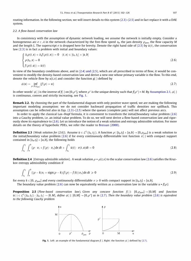
In view of the boundary conditions above, and in (2.4) and (2.5), which are all prescribed in terms of flow, it would be con-venient to modify the density-based conservation law and derive a new one whose primary variable is the flow. To this end,denote the vehicle flow by u(t,x) and consider the function g(%) defined by

/!u" $ infq2'0;qjam (

ff !q" $ ug !2:7"

In other words’ /(%) is the inverse of f(%) on [0,q⁄], where q⁄ is the unique density such that f(q⁄) =M. By Assumption 2.1, /(%)is continuous, convex and strictly increasing, see Fig. 1.

Remark 2.2. By choosing the part of the fundamental diagram with only positive wave speed, we are making the followingimportant modeling assumption: we do not consider backward propagation of traffic densities nor spillback. Thisassumption can be reflected also in Eqs. (2.3)–(2.5) where the queues (complete jam) will not affect previous arcs.

In order to apply the classical Lax–Hopf formula, it is convenient to transform the initial/boundary value problem (2.6)into a Cauchy problem, i.e. an initial value problem. To do so, we will next derive a flow-based conservation law and rigor-ously show its equivalence to (2.6). Let us introduce the notion of a weak solution and entropy admissible solution. For moredetails on the theory of hyperbolic PDEs, we refer the reader to Bressan (2000).

Definition 2.3 (Weak solution for (2.6)). Assume !u 2 L1!'t0; tf (". A function q: [t0, tf] ) [a,b]? [0,qjam] is a weak solution tothe initial/boundary value problem (2.6) if for every continuously differentiable test function v (%) with compact supportcontained in [t0, tf] ) [a,b], the following holds

Z tf

t0

Z b

afq % v t # f !q" % vxgdx dt #

Z tf

t0

!u!t" % v!t; a"dt $ 0 !2:8"

Definition 2.4 (Entropy admissible solution). A weak solution q = q(t,x) to the scalar conservation law (2.6) satisfies the Kruz-kov entropy admissibility condition if

Z tf

t0

Z b

afjq& kjv t # sign!q& k"!f !q" & f !k""vxgdx dt P 0 !2:9"

for every k 2 [0, qjam] and every continuously differentiable vP 0 with compact support in [t0, tf] ) [a,b].The boundary value problem (2.6) can now be equivalently written as a conservation law in the variable u = f(q):

Proposition 2.5 (Flow-based conservation law). Given any concave function f (%): [0,qjam]? [0,M] and function!u!%" 2 L1!'t0; tf (" : 't0; tf ( ! '0;M(, define /(%): [0,M]? [0,q⁄] as in (2.7). Then the boundary value problem (2.6) is equivalentto the following Cauchy problem

!*

!*

0 0!

!

u

u

M

M!jam

Fig. 1. Left: an example of the fundamental diagram f(%). Right: the function /(%) defined by (2.7).


@xu!t; x" # @t/!u!t; x"" $ 0 !x; t" 2 'a; b( ) 't0; tf (u!t; a" $ !u!t"

%!2:10"

where u(t,x) = f(q(t,x)).

Remark 2.6. Eq. (2.10) can be viewed as an initial value problem by switching the roles of variables t and x. The flow-basedPDE is easy to work with in terms of boundary conditions (2.4) and (2.5), and the initial value problem (2.10) immediatelyleads to the application of the Lax formula discussed in Evans (2010) and Lax (1957).

Proof. The proof is carried out by showing that q(t,x) is the entropy admissible weak solution of (2.6) if and only ifu(t,x) $: f(q(t,x)) is the entropy admissible weak solution of (2.10).

1. ‘‘only if ’’ part. We begin by arguing that the weak entropy solution q(t,x) of (2.6) satisfies q(t,x) 2 [0,q⁄], where q⁄ is theunique density such that f(q⁄) =M. This is because the characteristics emitting from the left boundary x = a must havenon-negative wave speed in order to influence the interior of the domain [t0, tf] ) [a,b]. Otherwise, if there exists!t; x" 2 !t0; tf ( ) !a; b"which is connected to the left boundary [t0, tf] ) {a} by a characteristic line with negative speed, thenq!t; x" is influenced by the boundary condition at a time > t, this contradicts the causality principle.Let q(%, %) be the weak entropy solution satisfying (2.8) and (2.9). By previous argument, there holds u = f(q), q = /(u). Thenwe readily deduce

0 $Z tf

t0

Z b

afq % v t # f !q" % vxgdx dt #

Z tf

t0

!u!t" % v!t; a"dt $Z tf

t0

Z b

af/!u" % v t # u % vxgdx dt #

Z tf

t0

!u!t" % v!t; a"dt

for any continuously differentiable v with compact support. This shows that u(t,x) is the weak solution to the initialvalue problem (2.10). In addition, let us fix arbitrary v(t,x)P 0 which is continuously differentiable and compactlysupported, for every s 2 [0,M], denote k = /(s) 2 [0, q⁄]. By the entropy condition (2.9)

0 6Z tf

t0

Z b

afjq& kjv t # sign!q& k"!f !q" & f !k"" vxgdx dt

$Z tf

t0

Z b

afj/!u" & /!s"jv t # sign!/!u" & /!s""!u& s" vxgdx dt

$Z tf

t0

Z b

afju& sjvx # sign!u& s" !/!u" & /!s""v tgdx dt

this implies u(%,%) is the entropy admissible solution to (2.10). Notice that the last equality above is by observing that /(%) is strictly increasing, thus

j/!u" & /!s"j $ sign!u& s"!/!u" & /!s""; ju& sj $ sign!/!u" & /!s""!u& s"

2. ‘‘if’’ part. The converse is completely similar, the key point is that q(t,x) 6 q⁄. Therefore f(q) = u, q = /(u). The rest of theverification is straightforward. h

It is well-established that a full LWR-based network model requires boundary conditions on both ends of the link, whichaccount for the propagation of upstream/downstream information. In our simplified model, in the absence of influence fromdownstream, the PDE for the link is constrained by just upstream boundary condition which must admit non-negative wavespeeds due to the causality principle.

We remind the reader that so far we have been dealing with the PDE (2.3) with boundary condition !u!t" given by (2.5).Such a boundary condition depends on the queue q(t) and the upstream flow profiles in a tricky way: (2.5) induces a discon-tinuous dependence of the ODE (2.4) on the variable q(t). In general, an ODE with a discontinuous right hand side is difficultto deal with both theoretically and computationally. For example, existence for the ODE is not guaranteed. In terms of com-putation, a finite difference scheme, whether forward or backward, could result in non-physical solutions such as negativequeue and negative flow. To overcome the aforementioned difficulties, we propose in the following a Hamilton–Jacobi equa-tion corresponding to the flow-based conservation law (2.10), and a modified Lax–Hopf formula which provides solution to(2.3)–(2.5).

2.3. Hamilton–Jacobi equation and Lax–Hopf formula for a homogeneous link

In this section, we will first introduce the Hamilton–Jacobi equation and the Lax formula for general Cauchy problems,then apply this to the flow-based conservation law (2.10) to obtain a semi-analytical characterization of the dynamics for


a homogeneous link. Initially introduced in Lax (1957, 1973), then extended in Aubin et al. (2008), Bardi and Capuzzo-Dolcetta (1997), and Le Floch (1988), and applied to traffic theory in Claudel and Bayen (2010a), Daganzo (2005, 2006),the Lax–Hopf formula provides a new characterization of the solution to the hyperbolic conservation law and Hamilton–Ja-cobi equation. The Lax formula is derived from the characteristics equations associated with the Hamilton–Jacobi PDE, whicharise in the classical calculus of variations and in mechanics, see Evans (2010) for a complete discussion.

Consider the initial value problem for the Hamilton–Jacobi equation

@tN !t; x" #H!@xN !t; x"" $ 0 !t; x" 2 !0;1" ) R

N !0; x" $ g!x" x 2 R

%!2:11"

where N : '0;#1" ) R ! R is the unknown, and H : R ! R is the Hamiltonian.

Theorem 2.7 (Lax–Hopf formula). Suppose H is continuous and convex, g!%" : R ! R is Lipschitz continuous, then

N !t; x" $ infy2R

tL x& yt

# $# g!y"

n o!2:12"

is the unique viscosity solution to the initial-value problem (2.11). Where L is the Legendre transformation of H:

L!q" $ infpfH!p" & qpg !2:13"

Proof. See Evans (2010). h

The Lax–Hopf formula expresses the viscosity solution of the Cauchy problem (2.11) as an optimization problem. In orderto transform the flow-based PDE (2.10) into the form (2.11), let us proceed as follows. Denote the cumulative vehicle countU!t; x"; U!t" by:

U!t; x" $Z t

t0

u!s; x"ds; U!t" $Z t

t0

!u!s"ds !2:14"

U(t,x) measures the cumulative count of vehicles that have passed the point x by time t, and U!t" measures the vehiclecount that have entered the link. In addition, we denote by Q(t) the count of vehicles that have arrived at the entrance ofthe link (possibly first joining a queue) by time t. In mathematical terms, if the arc is represented by the spatial interval[a,b], then

Q!t" $ U!t; a&"; U!t" $ U!t; a#"

Notice that by definition, U!%" must be Lipschitz continuous with constant M, this is because the rate at which cars enter thelink is bounded above by the flow capacity, i.e., !u!t" 6 M. Regarding Q(%), we assume the following:

A2. Q(%) is non-decreasing, left continuous with possibly countably many upward jumps.

Remark 2.8. In most traffic literature, the function which represent flow is usually assumed to be Lebesgue integrable. Con-sequently, the cumulative vehicle count – the anti-derivative of flow – is absolutely continuous. Therefore A2 generalizessuch assumption by allowing the cumulative count to be discontinuous. This corresponds to the situation where a positiveamount of cars enter the network at the same time. Although such circumstance is unlikely to happen in reality, it does arisein a mathematical context and demands proper treatment. See Bressan and Han (2011a) for an example where a disconti-nuity in the cumulative vehicle count is present in the DUE solution in continuous-time.

According to the rule (2.5), the relation between Q(%) and U!%" can be expressed by the following identity:

U!t" $ infs6t

fQ!s" #M!t & s"g !2:15"

By virtue of (2.15), U!t" 6 Q!t" and the difference measure the queue volume. Notice that (2.16) is precisely the integral formof (2.4) under the assumption that q(0) = 0.

q!t" $ Q!t" & U!t" !2:16"

We now introduce the integral form of (2.10), which is the following Hamilton–Jacobi equation:

@xU!t; x" # /!@t U!t; x"" $ 0 !x; t" 2 'a; b( ) 't0; tf (U!t; a" $ U!t"

(!2:17"

Note that (2.17) is in the form of a general Cauchy problem for the H–J equation in one dimension, i.e. (2.11). The onlydifference is the notation in which the roles of t and x are switched. With that in mind, we will next proceed to the Lax for-mula and derive analytical solutions to (2.17). Recall the following Legendre transformation:


Definition 2.9 (Legendre transformation). The Legendre (convex) transformation of convex function /(%): [0,M]? [0, q⁄] is

w!u" $: maxp

fpu& /!p"g !2:18"

It is easy to verify that the Legendre transform w(%) is convex and Lipschitz continuous with Lipschitz constant M. Next, weadapt the Lax–Hopf formula (2.12) to the Cauchy problem (2.17) and readily derive the following:

Proposition 2.10 (Lax–Hopf formula). Given convex function /(%) and its Legendre transform w(%), the viscosity solution U(t,x) to(2.17) satisfies

U!t; x" $ mins2R

U!s" # !x& a"w t & sx& a

& '% (; x 2 'a; b( !2:19"

In particular, the cumulative count of vehicles exiting the arc is given by:

U!t; b" $ mins2R

U!s" # Lwt & sL

& '% (!2:20"

Proof. Adjust the proof in Evans (2010) to the Cauchy problem (2.17). h

Remark 2.11. The original Lax–Hopf formula used infimum instead of minimum, but since all flows that we consider hereare compactly supported in [t0, tf], the infimum can be achieved within this compact set. Therefore, from now on, we will use‘‘min’’ instead of ‘‘inf’’.

As mentioned before, in a general network, the quantity Q(t) is easily recovered from upstream flow profiles. However,one cannot immediately apply formula (2.19) or (2.20) because U!%" is not explicitly given. One way to resolve this issueis to utilize identity (2.15), but this would require additional computational effort. Fortunately, the following lemma assertsthat this is not necessary and replacing U!%" with Q(%) will yield the same solution.

Proposition 2.12. Given the Lipschitz continuous function U!%" and function Q(%) satisfying Assumption 2.3, then the solutionU(t, b) satisfies

U!t; b" $ mins

U!s" # Lwt & sL

& '% ($ min

sQ!s" # Lw

t & sL

& '% (!2:21"

Proof. Introduce the function

j!s" $: & L w&sL

# $!2:22"

One can then easily verify that j(%) is a concave and Lipschitz continuous function with Lipschitz constant M. From formula(2.20) it now follows

U!t; b" $ mins

U!s" & j!s& t") *

!2:23"

Fix any t 2 [t0, tf], denote

s0 $ inf s* : U!s*" & j!s* & t" $ mins

fU!s" & j!s& t"gn o

!2:24"

Clearly s0 exists and satisfies U!s0" & j!s0 & t" $ minsfU!s" & j!s& t"g. Next we claim that

Q!s0" $ U!s0"

Otherwise if Q!s0" > U!s0", by left-continuity of Q(%), one must have Q!s" > U!s" for a small neighborhood s 2 [s0 & d, s0].Thus from (2.5) we deduce that d

dsU!s" $ M. By Lipschitz continuity of j(%) for s 2 [s0 & d, s0]

U!s" & j!s& t" & !U!s0" & j!s0 & t"" 6 0

contradicting (2.24). Thereby the claim is substantiated. The claim implies

mins

fQ!s" & j!s& t"g 6 Q!s0" & j!s0 & t" $ mins

fU!s" & j!s& t"g !2:25"

To show (2.25) with reversed inequality, one has only to notice Q!%" P U!%". h


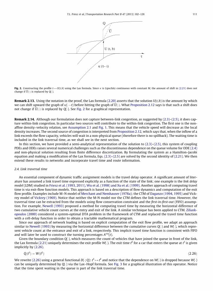
Remark 2.13. Using the notation in the proof, the Lax formula (2.20) asserts that the solution U(t,b) is the amount by whichwe can shift upward the graph of j(%&t) before hitting the graph of U!%". What Proposition 2.12 says is that such a shift doesnot change if U!%" is replaced by Q(%). See Fig. 2 for a graphical representation.

Remark 2.14. Although our formulation does not capture between-link congestion, as suggested by (2.3)–(2.5), it does cap-ture within-link congestion. In particular two sources will contribute to the within-link congestion. The first one is the non-affine density–velocity relation, see Assumption 2.1 and Fig. 1. This means that the vehicle speed will decrease as the localdensity increases. The second source of congestion is interpreted from Proposition 2.12, which says that, when the inflow of alink exceeds the flow capacity, vehicles will wait in a non-physical queue (therefore there is no spillback). The waiting time isincluded in the link traversal time, as we shall see in the next section.

In this section, we have provided a semi-analytical representation of the solution to (2.3)–(2.5), this system of couplingPDEs and ODEs raises several numerical challenges such as the discontinuous dependence on the queue volume for ODE (2.4)and non-physical solution resulting from finite difference discretization. By formulating the system as a Hamilton–Jacobiequation and making a modification of the Lax formula, Eqs. (2.3)–(2.5) are solved by the second identity of (2.21). We thenextend these results to networks and incorporate travel time and route information.

2.4. Link traversal time

An essential component of dynamic traffic assignment models is the travel delay operator. A significant amount of liter-ature has assumed a link travel time expressed explicitly as a function of the state of the link; one example is the link delaymodel (LDM) studied in Friesz et al. (1993, 2011), Wu et al. (1998) and Xu et al. (1999). Another approach of computing traveltime is via exit-flow function models. This approach is based on a description of flow dynamics and computation of the exitflow profile. Examples include M–Nmodel of Merchant and Nemhauser (1978a); the CTM of Daganzo (1994, 1995) and Vick-rey model of Vickrey (1969). Notice that neither the M-N model nor the CTM defines the link traversal time. However, thetraversal time can be extracted from the models using flow conservation constraint and the first-in-first-out (FIFO) assump-tion. For example, Newell (1993) proposed a method for computing travel time by measuring the horizontal difference oftwo cumulative vehicle count curves at the entry and exit of the link. A similar technique has been applied to CTM. Ziliask-opoulos (2000) considered a system-optimal DTA problem in the framework of CTM and replaced the travel time functionwith a cell-delay function in order to obtain a tractable mathematical program.

Since our approach of network loading is based on explicit computation of the exit flow profile, we adapt an approachsimilar to Newell (1993) by measuring the horizontal difference between the cumulative curves Q(%) and W(%), which repre-sent vehicle count at the entrance and exit of a link, respectively. This implicit travel time function is consistent with FIFOand will later be used to construct the turning percentages Av,e(t).

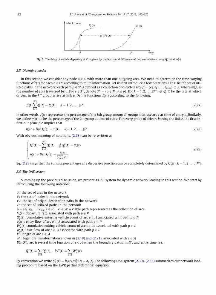
Given the boundary condition Q(%), which measures the count of vehicles that have joined the queue in front of the link,the Lax formula (2.21) uniquely determines the exit profile W(%). The exit time tE for a car that enters the queue at tS is givenimplicitly by (2.26).

Q!tS" $ W!tE" !2:26"

We rewrite (2.26) using a general functional D(%;Q): tS ´ tE and notice that the dependence on W(%) is dropped because W(%)can be uniquely determined by Q(%) via the Lax–Hopf formula. See Fig. 3 for a graphical illustration of this operator. Noticethat the time spent waiting in the queue is part of the link traversal time.

" (#$ t)

_U

#

U (t, b)

Q

Fig. 2. Constructing the profile t´ U(t,b) using the Lax formula. Since j is Lipschitz continuous with constant M, the amount of shift in (2.21) does notchange if U!%" is replaced by Q(%).


2.5. Diverging model

In this section we consider any node v 2 V with more than one outgoing arcs. We need to determine the time-varyingfunctions Av,e(t) for each e 2 Ov according to route information. Let us first introduce a few notations. Let P be the set of uti-lized paths in the network, each path p 2 P is defined as a collection of directed arcs p $ fe1; e2; . . . ; em!p"g + A, where m(p) isthe number of arcs traversed by p. For e 2 Iv , denote Pe $ fp 2 P : e 2 pg. For k $ 1;2; . . . ; jPej let qe

k!t" be the rate at whichdrivers in the kth group arrive at link e. Define functions nek!t" according to the following:

nek!t"XjPe j

l$1

qel !t" $ qe

k!t"; k $ 1;2; . . . ; jPej !2:27"

In other words, nek!t" represents the percentage of the kth group among all groups that use arc e at time of entry t. Similarly,we define ge

k!t" to be the percentage of the kth group at time of exit t. For every group of drivers k using the link e, the first-in-first-out principle implies that

gek!t # D!t;Qe"" $ nek!t"; k $ 1;2; . . . ; jPej !2:28"

With obvious meaning of notations, (2.28) can be re-written as

Qe!t" $XjPe j

k$1

Qek!t"; d

dt Qek!t" $ qe

k!t"

gek!t # D!t;Qe"" $ qek!t"PjPe j

l$1qel!t"

8>>><

>>>:!2:29"

Eq. (2.29) says that the turning percentages at a dispersive junction can be completely determined by Qek!t"; k $ 1;2; . . . ; jPej.

2.6. The DAE system

Summing up the previous discussion, we present a DAE system for dynamic network loading in this section. We start byintroducing the following notation:

A: the set of arcs in the networkV: the set of nodes in the networkW: the set of origin–destination pairs in the networkP: the set of utilized paths in the networkp $ fe1; e2; . . . ; em!p"g 2 P; ei 2 A: a viable path represented as the collection of arcshp(t): departure rate associated with path p 2 PQe

p!t": cumulative entering vehicle count of arc e 2 A associated with path p 2 Pqep!t": entry flow of arc e 2 A associated with path p 2 P

Wep!t":cumulative exiting vehicle count of arc e 2 A associated with path p 2 P

wep!t": exit flow of arc e 2 A associated with path p 2 P

Le: length of arc e 2 Awe: Legendre transformation shown in (2.18) and (2.21), associated with e 2 AD(t;Qe): arc traversal time function of e 2 A when the boundary datum is Qe, and entry time is t.

Qe!t" $:X

e2pQe

p!t"; We!t" $:X

e2pWei

p !t"

By convention we write qe1p !t" $ hp!t";we0

p !t" $ hp!t". The following DAE system (2.30)–(2.35) summarizes our network load-ing procedure based on the LWR partial differential equation:

SD (t ; Q)

vehicle countQ (t)

tS tA

W (t)

time

Fig. 3. The delay of vehicle departing at tS is given by the horizontal difference of two cumulative curves Q(%) and W(%).


Qe!t" $:X

e2pQe

p!t"; qe!t" $:X

e2pqep!t"; we!t" $:

X

e2pwe

p!t" !2:30"

ddt

Qep!t" $ qe

p!t";ddt

We!t" $ we!t"; 8p 2 P !2:31"

qeip !t" $ wei&1

p !t"; i 2 '1;m!p"(; p 2 P !2:32"

We!t" $ mins

Qe!s" # Lewe t & sLe

& '% (; 8e 2 A !2:33"

Qe!t" $ We!t # D!t; Qe""; 8e 2 A !2:34"

weip !t # D!t; Qei "" $

qeip !t"

qei !t"wei !t # D!t; Qei ""; i 2 '1;m!p"(; p 2 P !2:35"

We note that Eq. (2.30) is merely definitional, i.e. the traffic on an arc is disaggregated according to different route choices.Eq. (2.32) represents the fundamental recursion, which compels forward flow propagation to the next arc in the path. Eq.(2.33) is the Lax formula. Eq. (2.34) is often referred to as the flow propagation constraint. It determines the travel time func-tion D(%;Qe) in our case. Eq. (2.35) represents the diverging model in Section 2.5.Remark 2.15. We provide some insights regarding the existence and uniqueness of solutions to the above DAE system.Notice that the system does not contain any differential equations. The only equations involving differentiation are (2.31)and they are definitional. Moreover, the Lax–Hopf formula (2.33) provides the unique viscosity solution to the H–J equations.In addition, all variables of interests appear explicitly on the left hand side of the equations. This permits all variables to besolved for in sequential and in a pseudo cascading fashion. Therefore, the existence and uniqueness of solution to the DAEsystem is clear.

Remark 2.16. When we set out to solve the DNL submodel using a DAE system in the present paper, we are making anumerical approximation that can be as accurate as the modeler desires given sufficient computational resources. However,that numerical approximation should not be interpreted as an approximate DNL.

3. Formulation of the dynamic user equilibrium and Kuhn–Tucker conditions for the variational inequality

The dynamic network loading discussed in the previous section is viewed as the numerical procedure for evaluating theeffective delay operator, which is embedded in the definition of DUE proposed in Friesz et al. (1993). In this section we willre-visit the formulations of DUE as a variational inequality by Friesz et al. (1993), as a differential variational inequality byFriesz et al. (2001) and as a fixed-point problem by Friesz and Mookherjee (2006).

The goal of this section is as follows: (1) we wish to provide the readers with a comprehensive review of topics related tothe DUE and clear guidance on how to compute the DUE; and (2) we will utilize the Kuhn–Tucker conditions for finite-dimensional VIs to verify that the numerical solution we obtain is indeed the solution to the VI, and hence to the DUE prob-lem. To the authors’ knowledge this is the first attempt in the literature to test the numerical solutions against VI necessaryconditions. Thus the work in this section can serve as a reference to future researchers who are interested in the computa-tional aspects of DUE.

3.1. Dynamic user equilibrium formulation

We begin by considering a planning horizon 't0; tf ( + R. Let P be the set of paths employed by road users. The most crucialingredient of the DUE model is the path delay operator. Such an operator, denoted by

Dp!t;h" 8p 2 P

maps a given vector of departure rates h to the collection of travel times. Each travel time is associated with a particularchoice of route p 2 P and departure time t 2 [t0, tf]. The path delay operators usually do not take on any closed form, insteadthey can only be evaluated numerically through the dynamic network loading procedure. On top of the path delay operatorwe introduce the effective path delay operator which generalizes the notion of travel cost to include early or late arrival pen-alties. In this paper we consider the effective path delay operators of the following form

Wp!t;h" $ Dp!t;h" # F't # Dp!t;h" & TA( 8p 2 P !3:36"

where TA is the target arrival time. We introduce the fixed trip matrix Qij : !i; j" 2 W+ ,

, where each Qij 2 R# is the fixed traveldemand between origin–destination pair (i; j" 2 W. Note that Qij represents traffic volume, not flow. Finally we let Pij + P to


be the set of paths connecting origin–destination pair !i; j" 2 W. As mentioned earlier h is the vector of path flowsh $ fhp : p 2 Pg. We stipulate that each path flow is square integrable, that is

h 2 L2#'t0; tf (

+ ,jPj

The set of feasible path flows is defined as:

K0 $ h P 0 :X

p2Pij

Z tf

t0

hp!t"dt $ Qij 8!i; j" 2 W

8<

:

9=

;# L2#'t0; tf (# $jPj

!3:37"

Let us also define the essential infimum of effective travel delays

v ij $ essinf'Wp!t; h" : p 2 Pij( 8!i; j" 2 W

The following definition of dynamic user equilibrium was first articulated by Friesz et al. (1993)

Definition 3.1 (Dynamic user equilibrium). A vector of departure rates (path flows) h⁄ 2K0 is a dynamic user equilibrium if

h*p!t" > 0;p 2 Pij ) Wp't; h*!t"( $ v ij

We denote this equilibrium by DUE(W,K0,[t0,tf]).Using measure theoretic arguments, Friesz et al. (1993) established that a dynamic user equilibrium is equivalent to the

following variational inequality under suitable regularity conditions:

find h* 2 K0 such thatX

p2P

R tft0Wp!t; h*" hp & h*

p

# $dt P 0

8h 2 K0

9>>>=

>>>;VI!W;K0; 't0; tf (" !3:38"

It has been noted in Friesz et al. (2001) that (3.38) is equivalent to a differential variational inequality. This is most easilyseen by noting that the flow conservation constraints may be re-stated as:

dyijdt $

X

p2Pij

hp!t"

yij!t0" $ 0yij!tf " $ Qij

9>>>=

>>>;8!i; j" 2 W

which is recognized as a two point boundary value problem. As a consequence, (3.38) may be expressed as the following DVI:

find h* 2 K such thatX

p2P

R tft0Wp!t; h*" hp & h*

p

# $dt P 0

8h 2 K

9>>=

>>;DVI!W;K; 't0; tf (" !3:39"

where

K $ h P 0 :dyijdt

$X

p2Pij

hp!t"; yij!t0" $ 0; yij!tf " $ Qij 8 !i; j" 2 W

8<

:

9=

; !3:40"

Finally, we are in a position to state a result that permits the solution of the DVI (3.39) to be obtained by solving a fixed pointproblem.2

Theorem 3.2 (Fixed point re-statement). Assume that Wp!%;h" : 'to; tf ( ! R# is measurable for all p 2 P;h 2 K. Then the fixedpoint problem

h* $ PK h* & aW!t; h*"' ( !3:41"

is equivalent to DVI(W,K,D) where PK[%] is the minimum norm projection onto K and a 2 R#.

Proof. See Friesz (2010). h

2 The fixed-point iteration scheme should not be confused with simulation-based approaches since our iterations are merely approximations that aresuccessively refined until convergence produces a realized system state; that is, iterations prior to convergence have no physical meaning. This is in contrast tosimulation where each iteration of a simulation model produces a representation of a system state or scenario at a particular point in time. Such states areintended to directly map onto the physical world typically with associated performance measures.


3.2. Solution algorithm based on the fixed-point iterations

The fixed-point problem (3.41) can be instantiated as the following linear-quadratic optimal control problem

h* $ argminh

12

h* & aW!t; h*" & hk k : h 2 K% (

!3:42"

Then we can write the fixed point sub-problem at the kth iteration as follows

hk#1 $ argminh

12khk & aW!t;hk" & hk2 : h 2 K

% (!3:43"

That is, we seek the solution of the optimal control problem

minh

Jk!h" $X

!i;j"2Wv ij'Qij & yij!tf "( #

X

!i;j"2W

X

p2Pij

Z tf

t0

12

hkp & aWp!t; h" & hp

h i2!3:44"

subject to:

dyijdt

$X

p2Pij

hp!t" 8!i; j" 2 W !3:45"

yij!t0" $ 0 8!i; j" 2 W !3:46"h P 0 !3:47"

Finding dual variables associated with terminal time demand constraints turns out to be relatively easy. Note that the rel-evant Hamiltonian for (3.44)–(3.47) is:

Hk $ 12

m!i;j"2W

X

p2Pij

hkp & aWp!t; hk" & hp

h i2#

X

!i;j"2W

kijX

p2Pij

hp !3:48"

where each kij is an adjoint variable obeying

dkijdt

$ !&1" @Hk

@yij$ 0 8!i; j" 2 W

kij!tf " $@v ij'Qij & yij!tf "(

@yij!tf "$ &v ij 8!i; j" 2 W

From the above we determine that

kij!t" , &v ij 8t 2 't0; tf (; !i; j" 2 W

The minimum principle implies for any p 2 P,

hk#1p !t" $ arg

@Hk

@hp$ 0

( )

$ arg hkp!t" & aWp!t;hk" & hp!t"

# $h i!&1" & v ij $ 0

n o

Thus we obtain

hk#1p !t" $ hk

p!t" & aWp t;hk# $

# v ij

h i

#8!i; j" 2 W;p 2 Pij !3:49"

Notice that the following flow conservation constraint applies here.

X

p2Pij

Z tf

t0

hk#1p !t"dt $ Qij 8!i; j" 2 W

Consequently the dual variable vij must satisfy

X

p2Pij

Z tf

t0

hkp!t" & aWp!t; hk" # v ij

h i

#dt $ Qij 8!i; j" 2 W !3:50"

Recalling that each vij is time invariant and noticing that the equations of (3.50) are uncoupled, we see that simple linesearches will find the value of vij satisfying the above conditions. Once the vij’s are determined, the new vector of path flowshk+1 for the next iteration may be computed from (3.49).

Remark 3.3. The fixed-point iteration (3.43) is clearly a particular instance of the abstract algorithm xk+1 =M(xk) for solvingthe fixed point problem x⁄ =M(x⁄). However, such an algorithm does not enjoy a general theorem assuring strong


convergence of {xk}, even when M(%) is non-expansive. This is so because the effective delay operator is not stronglymonotone or component-wise strongly pseudomonotone delay operators. Further analytical properties need to beextracted from the current model to shed more light on the convergence issue. This has been left as future research. Itshould be noted that in all the numerical studies we present below, the fixed-point iterations do meet the convergencecriteria, that is

khk#1 & hkkL2khkkL2

6 e; for some k !3:51"

where e is some user-defined threshold.

3.3. Kuhn–Tucker condition for finite-dimensional VIs

This section focuses on the variational inequality (3.38), to derive a finite-dimensional version of VI (3.38), we introduce auniform time grid with step size Dt:

t0 $ t1 < t2 < % % % < tn $ tf !3:52"

We will use this notation:

!hp;i $: hp!ti" 2 R; !hp $

: !!hp;i"ni$1 2 Rn; !h $: !!hp"p2P 2 Rn)jPj;

Wp;i!!h" $: Wp!ti;h"; Wp!!h" $

: Wp;i!!h"+ ,n

i$1 2 Rn W!!h" $: Wp!!h"+ ,

p2P 2 Rn)jPj

Q $ !Qij"!i;j"2W 2 RjWj

Next we apply rectangular quadrature for the approximation of integrals, then the discrete-time version of inequality in(3.38) becomes

X

p2PDtWp!!h*"T !hp & !h*

p

# $P 0 () W!!h*"T!!h& !h*" P 0

The flow conservation constraints becomeX

p2Pij

DteT!hp $ Qij; 8!i; j" 2 W

where e 2 Rn is the vector of ones. We now introduce the following compact notation

a!%" : Rn)jPj ! Rn)jPj; a!!h" $ &!h !3:53"b!%" : Rn)jPj ! Rn)jPj; b!!h" $ A % !h& Q=Dt !3:54"

where each row of the matrix A 2 RjWj)njPj has ones located at the spots corresponding to OD pair (i, j) and zeros elsewhere.K0 can be rewritten as:

K0 $ f!h 2 Rn)jPj : a!!h" 6 0; b!!h" $ 0g

We now we are ready to state the discrete-time variational inequality VI!W;K0; 't0; tf (" and the necessary condition for thisfinite-dimensional VI:

find !h* 2 K0 such thatW!!h*"T!!h& !h*" P 08!h 2 K0

9>=

>;VI!W;K0; 't0; tf (" !3:55"

where

K0 $ !h 2 Rn)jPj : a!!h" 6 0; b!!h" $ 0) *

!3:56"

Theorem 3.4. (Kuhn–Tucker conditions for VI!W;K0; 't0; tf ("). Let

!h* 2 K0 $ !h 2 Rn)jPj : a!!h" 6 0; b!!h" $ 0) *

be a solution of (3.55). Further assume thatW!%" and a(%) are continuous on K0;a!%" is differentiable on K0, and b(%) is affine on K0.Then if the gradients rai!!h*" for i such that gi!!h*" $ 0 together with the gradients rbi!!h*" for i $ 1; . . . ;n) jPj are linearly inde-pendent, there exists multipliers p 2 Rn)jPj and l 2 Rn)jPj such that


W!!h*" # 'ra!!h*"(Tp# 'rb!!h*"(Tl $ 0 !3:57"piai!!h*" $ 0; i $ 1; . . . ;n) jPj !3:58"pP 0 !3:59"

Proof. See Friesz (2010). h

Remark 3.5. The functions a(%), b(%) clearly satisfy the assumption of the above theorem. Regarding the continuity of theeffective delay operatorW(%, %) in continuous time, we refer the readers to Bressan and Han (2012) for a proof. The continuityof W!%" in Theorem 3.4 follows directly from the continuity of W(%, %). We further comment that the necessary conditions forthe VI become sufficient if in addition the constraint functions a(%) are convex, which is again true in our case.

Next, we will transform condition (3.59) and (3.57) into a linear system. Note

ra!!h*" $ &I; rb!!h*" $ A

where I is the njPj) njPj identity matrix. Let X $ diag!&!h*" 2 RnjPj)njPj, Eqs. (3.59) and (3.57) is equivalent to the followinglinear system

&I AX 0

- . pl

- .$ &W!!h*"

0

" #!3:60"

In order to verify the sufficient and necessary condition (3.57)–(3.59), one needs to solve the above system and verify thatthe dual variables pP 0. Notice that the size of such system is 2njPj) !njPj# jWj" which could be very large.The Sioux Fallsnetwork example presented in Section 4.5 has 496 O–D pairs and 1941 paths. A chosen time grid of 100 points will lead to a400,000)200,500 linear system. Such a large system will cause the solution procedure to significantly slow down and evencrash if the system is not well-conditioned. We present our resolution to this issue with a decomposition of the system (3.60)summarized in the next lemma.

Lemma 3.6 (Decomposition of the linear system). For i $ 1; . . . ; jWj, denote by Wi!!h*";pi;li the vectors formed by selecting therows corresponding to the ith OD pair of the original vectors; denote by Ii,Ai, Xi the submatrices formed by selecting the rows andcolomns corresponding to the ith OD pair of the original matrices. The linear system (3.60) is then equivalent to a collection ofsmaller systems

&Ii Ai

Xi 0

" #pi

li

" #$ &Wi!!h*"

0

" #i $ 1; . . . ; jWj !3:61"

Proof. The conclusion follows from a simple block matrix arithmetic. h

Each system in (3.61) is much smaller in size, however, one may have to solve such linear systems as many times as thenumber of OD pairs. This strategy is particularly useful when computer memory is insufficient for large-scale computation.

4. Numerical examples

In this section, we present several numerical studies of the proposed DNL procedure formulated as a DAE system (2.30)–(2.35). In particular, we consider four different vehicular networks of varying sizes and topologies, as summarized in Table 1.All computations of the DNL procedure and fixed-point iteration presented in this section were coded in Matlab 2010 andperformed on a 2.7 GHz 4 GB of RAM computer. Every attempt was made to avoid the use of numerical tricks that couldnot be equally applied to all models. For the numerical results of the DNL, the LWR-based DAE system presented in this paperdisplays different flow propagation patterns from the LDM and CTM link performance models studied in Friesz et al. (2011).The solutions for the latter are moving parabolic wave forms, while the solutions of our DNL procedure display the non-uni-formity of wave speeds – a key feature of kinematic wave models. This is best explained by the flux function /(%) defined in(2.7), which implies that the higher the flow, the slower it propagates. This property will be visualized in Section 4.3.

4.1. Numerical context

For all numerical examples presented in this section, we fixed the time horizon [0,20]. The effective delay takes on thefollowing form

Wp!t;h" $ Dp!t;h" # c) !t # Dp!t; h" & TA"2

where Dp(t,h) is the network delay operator for path p 2 P and TA is the target arrival time. We assumed that there is a qua-dratic penalty for arrivals other than the desired time. The parameter c 2 R# measures the network users’ perception of ar-


rival penalties and is allowed to depend on different user classes. As the initial iterate of the fixed-point algorithm, we utilizean inverse parabolic-shaped initial departure rate. Note that an appropriate pre-condition, such as a different initial guessesmay improve the performance of the fixed-point algorithm, but this is beyond the scope of this paper. Finally, the conver-gence criteria of the fixed-point algorithm was set to be (3.51).

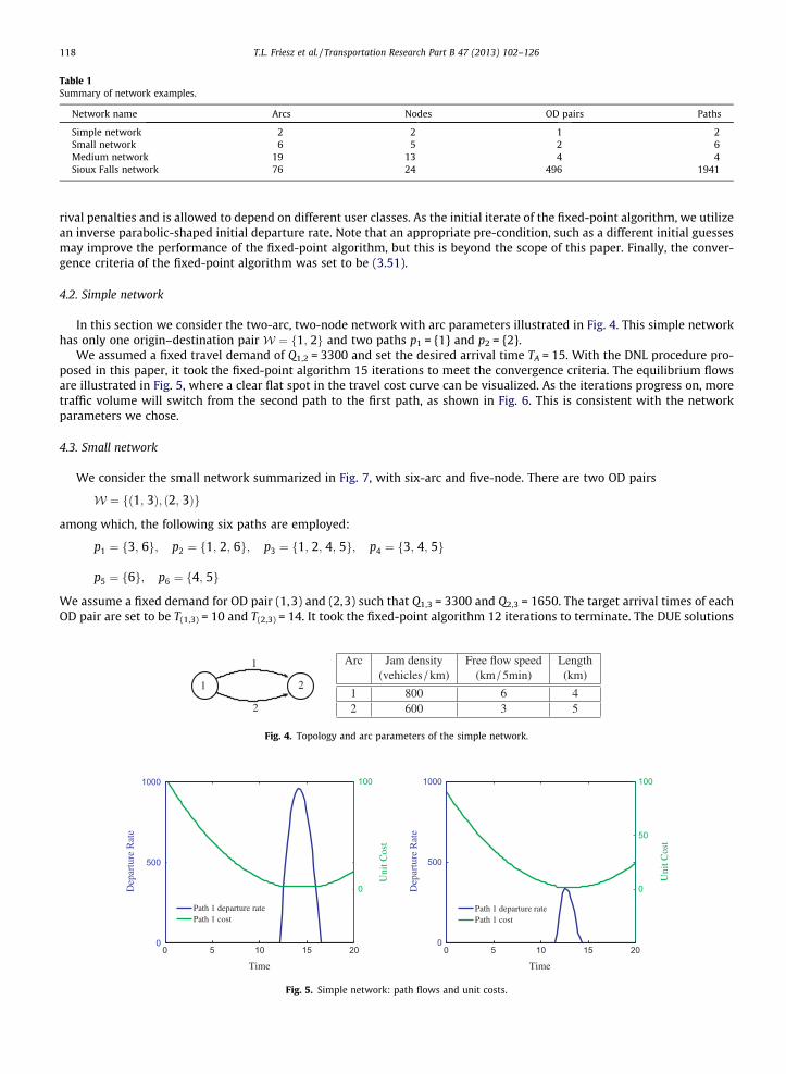
4.2. Simple network

In this section we consider the two-arc, two-node network with arc parameters illustrated in Fig. 4. This simple networkhas only one origin–destination pair W $ f1; 2g and two paths p1 = {1} and p2 = {2}.

We assumed a fixed travel demand of Q1,2 = 3300 and set the desired arrival time TA = 15. With the DNL procedure pro-posed in this paper, it took the fixed-point algorithm 15 iterations to meet the convergence criteria. The equilibrium flowsare illustrated in Fig. 5, where a clear flat spot in the travel cost curve can be visualized. As the iterations progress on, moretraffic volume will switch from the second path to the first path, as shown in Fig. 6. This is consistent with the networkparameters we chose.

4.3. Small network

We consider the small network summarized in Fig. 7, with six-arc and five-node. There are two OD pairs

W $ f!1; 3"; !2; 3"g

among which, the following six paths are employed:

p1 $ f3; 6g; p2 $ f1; 2; 6g; p3 $ f1; 2; 4; 5g; p4 $ f3; 4; 5g

p5 $ f6g; p6 $ f4; 5g

We assume a fixed demand for OD pair (1,3) and (2,3) such that Q1,3 = 3300 and Q2,3 = 1650. The target arrival times of eachOD pair are set to be T(1,3) = 10 and T(2,3) = 14. It took the fixed-point algorithm 12 iterations to terminate. The DUE solutions

Table 1Summary of network examples.

Network name Arcs Nodes OD pairs Paths

Simple network 2 2 1 2Small network 6 5 2 6Medium network 19 13 4 4Sioux Falls network 76 24 496 1941

Fig. 4. Topology and arc parameters of the simple network.

00

500

1000

Time

Dep

artu

re R

ate

5 10 15 20

0

100

Uni

t Cos

t

0

500

1000

Time

Dep

artu

re R

ate

0 5 10 15 20

0

50

100

Uni

t Cos

t

Path 1 departure ratePath 1 cost

Path 1 departure ratePath 1 cost

Fig. 5. Simple network: path flows and unit costs.


are shown in Fig. 8. We note that the curve corresponding to travel cost is flat where the departure rate is nonzero. Fig. 9shows the propagation of several path flows along each arc. As mentioned at the beginning of this section, the LWR-basedmodels tend to display non-uniform wave speeds, i.e. the part of the flow profile with relatively high value will propagatemore slowly than the part with low value.

1 2 3 4 5 6 7 8 9 10 11 12 13 14 150

500

1000

1500

2000

2500

3000

Iteration

Path

Allo

catio

n

Path 1 Volume

Path 2 Volume

Fig. 6. Path allocations during each fixed-point iteration.

Fig. 7. Topology and arc parameters of the small network.

0 2 4 6 8 10 12 14 16 18 200

500

1000

Time

Dep

artu

re R

ate

0

100

200

300

Uni

t Cos

t

0 2 4 6 8 10 12 14 16 18 200

500

1000

Time

Dep

artu

re R

ate

0

100

200

300

Uni

t Cos

t

0 2 4 6 8 10 12 14 16 18 200

500

1000

Time

Dep

artu

re R

ate

0

100

200

300

Uni

t Cos

t

0 2 4 6 8 10 12 14 16 18 200

500

1000

Time

Dep

artu

re R

ate

0

100

200

300

Uni

t Cos

t

0 2 4 6 8 10 12 14 16 18 200

500

1000

Time

Dep

artu

re R

ate

0

100

200

300

Uni

t Cos

t

0 2 4 6 8 10 12 14 16 18 200

500

1000

Time

Dep

artu

re R

ate

0

100

200

300

Uni

t Cos

t

Path 6 departure rate Path 6 costPath 5 departure rate Path 5 cost



Fig. 8. Small network: the six path departure rates and corresponding travel cost in the DUE solution.


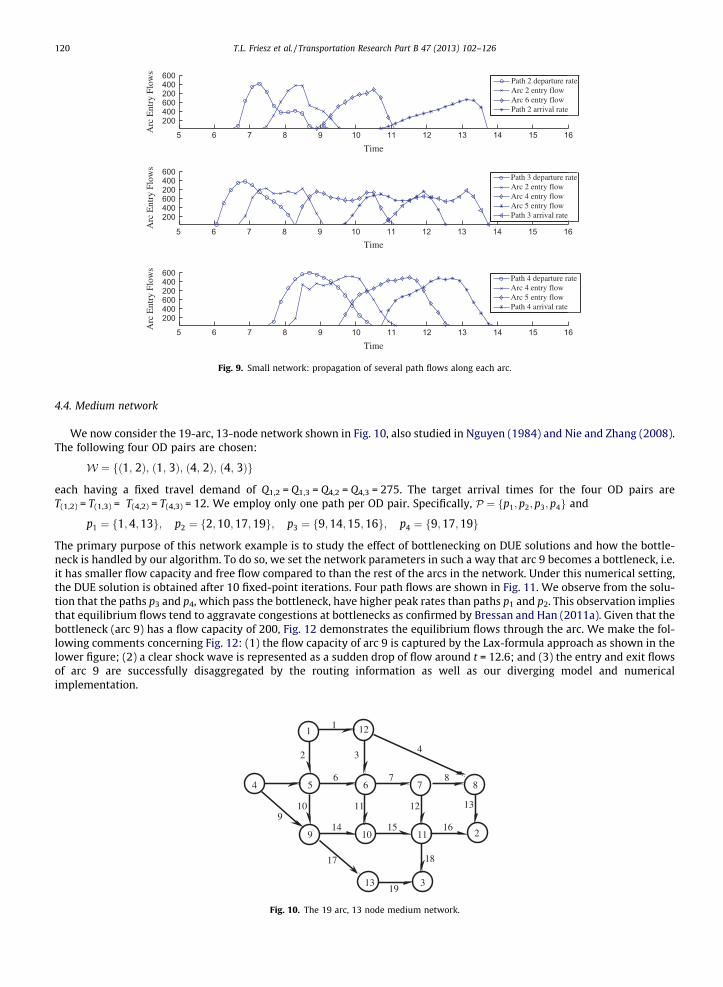
4.4. Medium network

We now consider the 19-arc, 13-node network shown in Fig. 10, also studied in Nguyen (1984) and Nie and Zhang (2008).The following four OD pairs are chosen:

W $ f!1; 2"; !1; 3"; !4; 2"; !4; 3"g

each having a fixed travel demand of Q1,2 = Q1,3 = Q4,2 = Q4,3 = 275. The target arrival times for the four OD pairs areT(1,2) = T(1,3) = T(4,2) = T(4,3) = 12. We employ only one path per OD pair. Specifically, P $ fp1; p2; p3; p4g and

p1 $ f1;4;13g; p2 $ f2;10;17;19g; p3 $ f9;14;15;16g; p4 $ f9;17;19g

The primary purpose of this network example is to study the effect of bottlenecking on DUE solutions and how the bottle-neck is handled by our algorithm. To do so, we set the network parameters in such a way that arc 9 becomes a bottleneck, i.e.it has smaller flow capacity and free flow compared to than the rest of the arcs in the network. Under this numerical setting,the DUE solution is obtained after 10 fixed-point iterations. Four path flows are shown in Fig. 11. We observe from the solu-tion that the paths p3 and p4, which pass the bottleneck, have higher peak rates than paths p1 and p2. This observation impliesthat equilibrium flows tend to aggravate congestions at bottlenecks as confirmed by Bressan and Han (2011a). Given that thebottleneck (arc 9) has a flow capacity of 200, Fig. 12 demonstrates the equilibrium flows through the arc. We make the fol-lowing comments concerning Fig. 12: (1) the flow capacity of arc 9 is captured by the Lax-formula approach as shown in thelower figure; (2) a clear shock wave is represented as a sudden drop of flow around t = 12.6; and (3) the entry and exit flowsof arc 9 are successfully disaggregated by the routing information as well as our diverging model and numericalimplementation.

5 6 7 8 9 10 11 12 13 14 15 16

200400600200400600

TimeA

rc E

ntry

Flo

ws

5 6 7 8 9 10 11 12 13 14 15 16

200400600200400600

Time

Arc

Ent

ry F

low

s

5 6 7 8 9 10 11 12 13 14 15 16

200400600200400600

Time

Arc

Ent

ry F

low

s

Path 2 departure rateArc 2 entry flowArc 6 entry flowPath 2 arrival rate

Path 3 departure rateArc 2 entry flowArc 4 entry flowArc 5 entry flowPath 3 arrival rate

Path 4 departure rateArc 4 entry flowArc 5 entry flowPath 4 arrival rate

Fig. 9. Small network: propagation of several path flows along each arc.

1 12

6 7

211

13

10

4

1

159

14

854

9

3

32

6

10 11 12 13

16

87

17

19

18

Fig. 10. The 19 arc, 13 node medium network.


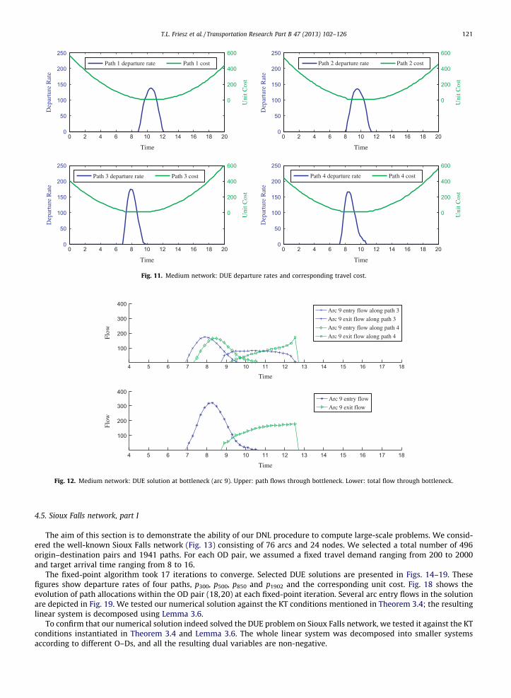
4.5. Sioux Falls network, part I

The aim of this section is to demonstrate the ability of our DNL procedure to compute large-scale problems. We consid-ered the well-known Sioux Falls network (Fig. 13) consisting of 76 arcs and 24 nodes. We selected a total number of 496origin–destination pairs and 1941 paths. For each OD pair, we assumed a fixed travel demand ranging from 200 to 2000and target arrival time ranging from 8 to 16.

The fixed-point algorithm took 17 iterations to converge. Selected DUE solutions are presented in Figs. 14–19. Thesefigures show departure rates of four paths, p300, p500, p850 and p1902 and the corresponding unit cost. Fig. 18 shows theevolution of path allocations within the OD pair (18,20) at each fixed-point iteration. Several arc entry flows in the solutionare depicted in Fig. 19. We tested our numerical solution against the KT conditions mentioned in Theorem 3.4; the resultinglinear system is decomposed using Lemma 3.6.

To confirm that our numerical solution indeed solved the DUE problem on Sioux Falls network, we tested it against the KTconditions instantiated in Theorem 3.4 and Lemma 3.6. The whole linear system was decomposed into smaller systemsaccording to different O–Ds, and all the resulting dual variables are non-negative.

0 2 4 6 8 10 12 14 16 18 200

50

100

150

200

250

Time

Dep

artu

re R

ate

0

200

400

600

Uni

t Cos

t

0 2 4 6 8 10 12 14 16 18 200

50

100

150

200

250

Time

Dep

artu

re R

ate

0

200

400

600

Uni

t Cos

t

0 2 4 6 8 10 12 14 16 18 200

50

100

150

200

250

Time

Dep

artu

re R

ate

0

200

400

600

Uni

t Cos

t0 2 4 6 8 10 12 14 16 18 20

0

50

100

150

200

250

TimeD

epar

ture

Rat

e

0

200

400

600

Uni

t Cos

t

Path 1 departure rate Path 1 cost Path 2 departure rate Path 2 cost

Path 3 departure rate Path 3 cost Path 4 departure rate Path 4 cost

Fig. 11. Medium network: DUE departure rates and corresponding travel cost.

4 5 6 7 8 9 10 11 12 13 14 15 16 17 18

100

200

300

400

Time

Flow

4 5 6 7 8 9 10 11 12 13 14 15 16 17 18

100

200

300

400

Time

Flow

Arc 9 entry flow along path 3Arc 9 exit flow along path 3Arc 9 entry flow along path 4Arc 9 exit flow along path 4

Arc 9 entry flowArc 9 exit flow

Fig. 12. Medium network: DUE solution at bottleneck (arc 9). Upper: path flows through bottleneck. Lower: total flow through bottleneck.


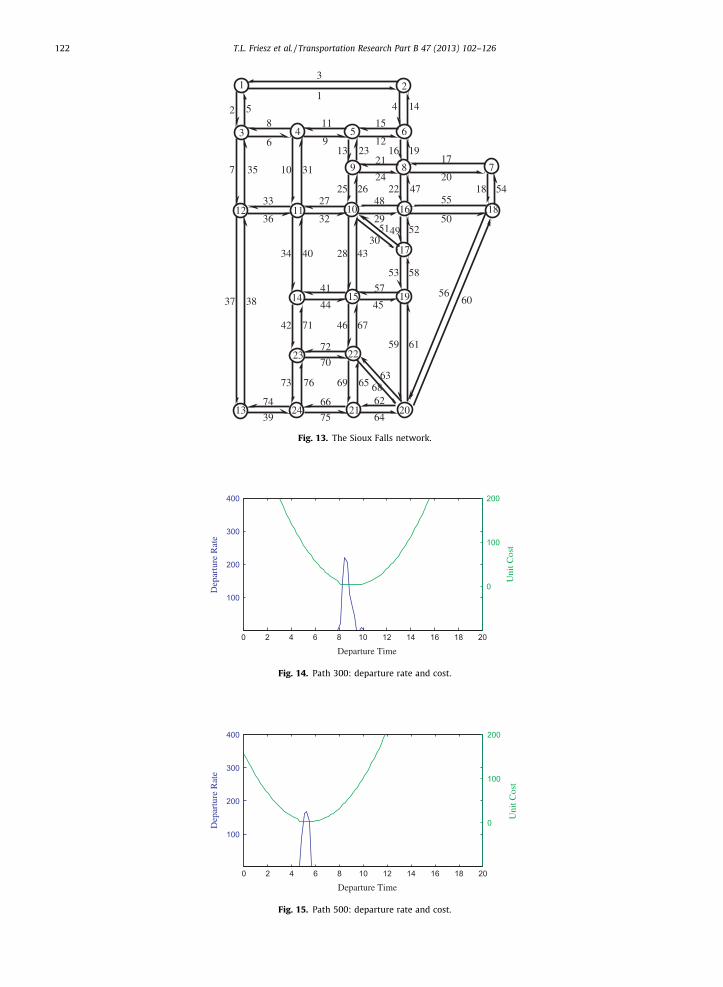
Fig. 13. The Sioux Falls network.

0 2 4 6 8 10 12 14 16 18 20

200

400

100

300

Departure Time

Dep

artu

re R

ate

0

100

200U

nit C

ost

Fig. 14. Path 300: departure rate and cost.

0 2 4 6 8 10 12 14 16 18 20

200

400

100

300

Departure Time

Dep

artu

re R

ate

0

100

200

Uni

t Cos

t



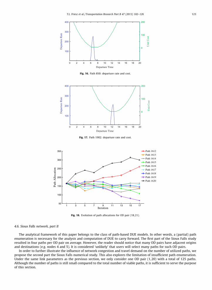
4.6. Sioux Falls network, part II

The analytical framework of this paper belongs to the class of path-based DUE models. In other words, a (partial) pathenumeration is necessary for the analysis and computation of DUE to carry forward. The first part of the Sioux Falls studyresulted in four paths per OD pair on average. However, the reader should notice that many OD pairs have adjacent originsand destinations (e.g. nodes 4 and 5). It is considered ‘unlikely’ that users will select many paths for such OD pairs.

In order to further illustrate the influence of network congestion and travel demand on the number of utilized paths, wepropose the second part the Sioux Falls numerical study. This also explores the limitation of insufficient path enumeration.Under the same link parameters as the previous section, we only consider one OD pair (1,20) with a total of 125 paths.Although the number of paths is still small compared to the total number of viable paths, it is sufficient to serve the purposeof this section.

0 2 4 6 8 10 12 14 16 18 20

300

200

400

100

Departure Time

Dep

artu

re R

ate

0

100

200

Uni

t Cos

t


0 2 4 6 8 10 12 14 16 18 20

200

400

100

300

Departure Time

Dep

artu

re R

ate

0

100

200

Uni

t Cos

t


1 3 5 7 9 11 13 15 1750

100

150

200

250

300

350

Iteration

Path

Alloc

ation

Path 1612Path 1613Path 1614Path 1615Path 1616Path 1617Path 1618Path 1619Path 1620

Fig. 18. Evolution of path allocations for OD pair (18,21).


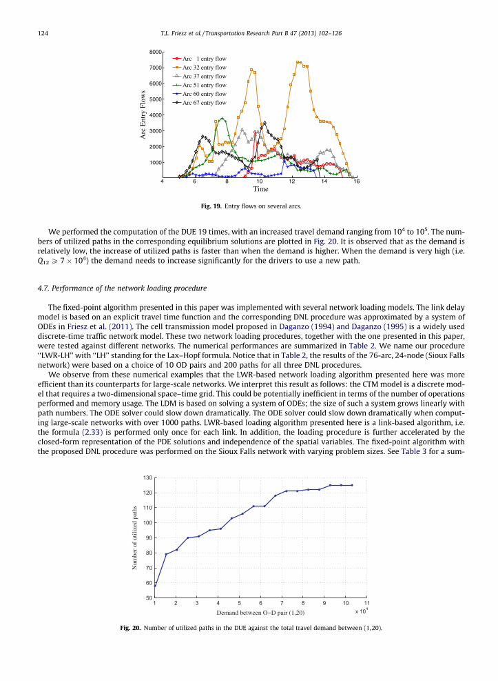
We performed the computation of the DUE 19 times, with an increased travel demand ranging from 104 to 105. The num-bers of utilized paths in the corresponding equilibrium solutions are plotted in Fig. 20. It is observed that as the demand isrelatively low, the increase of utilized paths is faster than when the demand is higher. When the demand is very high (i.e.Q12 P 7 ) 104) the demand needs to increase significantly for the drivers to use a new path.

4.7. Performance of the network loading procedure

The fixed-point algorithm presented in this paper was implemented with several network loading models. The link delaymodel is based on an explicit travel time function and the corresponding DNL procedure was approximated by a system ofODEs in Friesz et al. (2011). The cell transmission model proposed in Daganzo (1994) and Daganzo (1995) is a widely useddiscrete-time traffic network model. These two network loading procedures, together with the one presented in this paper,were tested against different networks. The numerical performances are summarized in Table 2. We name our procedure‘‘LWR-LH’’ with ‘‘LH’’ standing for the Lax–Hopf formula. Notice that in Table 2, the results of the 76-arc, 24-node (Sioux Fallsnetwork) were based on a choice of 10 OD pairs and 200 paths for all three DNL procedures.

We observe from these numerical examples that the LWR-based network loading algorithm presented here was moreefficient than its counterparts for large-scale networks. We interpret this result as follows: the CTMmodel is a discrete mod-el that requires a two-dimensional space–time grid. This could be potentially inefficient in terms of the number of operationsperformed and memory usage. The LDM is based on solving a system of ODEs; the size of such a system grows linearly withpath numbers. The ODE solver could slow down dramatically. The ODE solver could slow down dramatically when comput-ing large-scale networks with over 1000 paths. LWR-based loading algorithm presented here is a link-based algorithm, i.e.the formula (2.33) is performed only once for each link. In addition, the loading procedure is further accelerated by theclosed-form representation of the PDE solutions and independence of the spatial variables. The fixed-point algorithm withthe proposed DNL procedure was performed on the Sioux Falls network with varying problem sizes. See Table 3 for a sum-

4 6 8 10 12 14 16

1000

2000

3000

4000

5000

6000

7000

8000

Time

Arc E

ntry F

lows

Arc 1 entry flowArc 32 entry flowArc 37 entry flowArc 51 entry flowArc 60 entry flowArc 67 entry flow

Fig. 19. Entry flows on several arcs.

1 2 3 4 5 6 7 8 9 10 11x 104

50

60

70

80

90

100

110

120

130

Demand between O!D pair (1,20)

Num

ber o

f util

ized

pat

hs

Fig. 20. Number of utilized paths in the DUE against the total travel demand between (1,20).


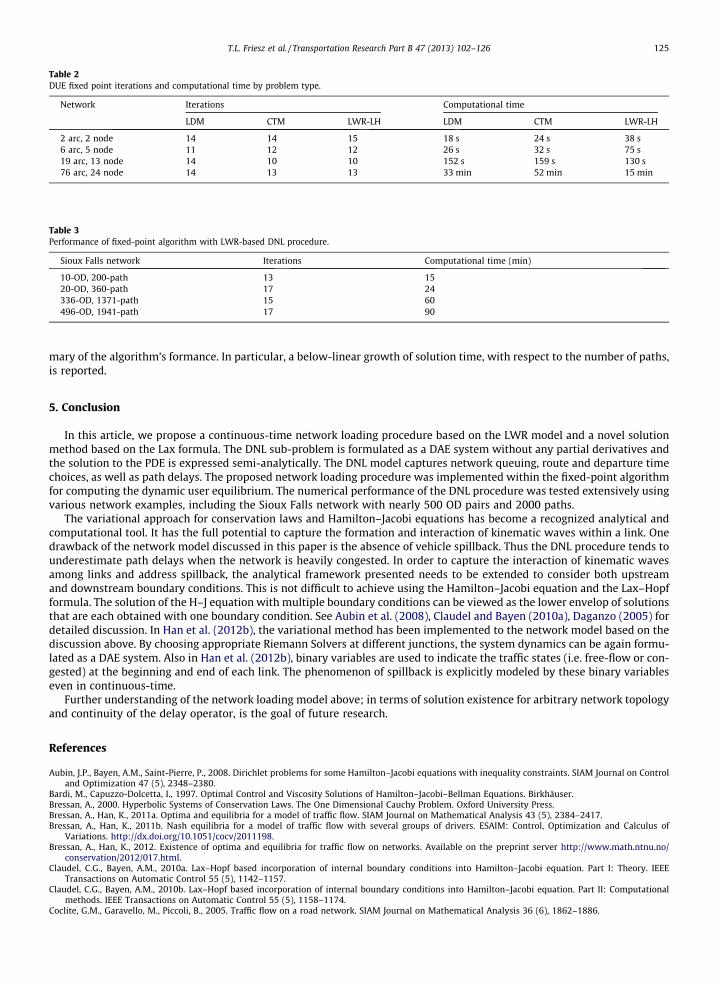
mary of the algorithm’s formance. In particular, a below-linear growth of solution time, with respect to the number of paths,is reported.

5. Conclusion

In this article, we propose a continuous-time network loading procedure based on the LWR model and a novel solutionmethod based on the Lax formula. The DNL sub-problem is formulated as a DAE system without any partial derivatives andthe solution to the PDE is expressed semi-analytically. The DNL model captures network queuing, route and departure timechoices, as well as path delays. The proposed network loading procedure was implemented within the fixed-point algorithmfor computing the dynamic user equilibrium. The numerical performance of the DNL procedure was tested extensively usingvarious network examples, including the Sioux Falls network with nearly 500 OD pairs and 2000 paths.

The variational approach for conservation laws and Hamilton–Jacobi equations has become a recognized analytical andcomputational tool. It has the full potential to capture the formation and interaction of kinematic waves within a link. Onedrawback of the network model discussed in this paper is the absence of vehicle spillback. Thus the DNL procedure tends tounderestimate path delays when the network is heavily congested. In order to capture the interaction of kinematic wavesamong links and address spillback, the analytical framework presented needs to be extended to consider both upstreamand downstream boundary conditions. This is not difficult to achieve using the Hamilton–Jacobi equation and the Lax–Hopfformula. The solution of the H–J equation with multiple boundary conditions can be viewed as the lower envelop of solutionsthat are each obtained with one boundary condition. See Aubin et al. (2008), Claudel and Bayen (2010a), Daganzo (2005) fordetailed discussion. In Han et al. (2012b), the variational method has been implemented to the network model based on thediscussion above. By choosing appropriate Riemann Solvers at different junctions, the system dynamics can be again formu-lated as a DAE system. Also in Han et al. (2012b), binary variables are used to indicate the traffic states (i.e. free-flow or con-gested) at the beginning and end of each link. The phenomenon of spillback is explicitly modeled by these binary variableseven in continuous-time.

Further understanding of the network loading model above; in terms of solution existence for arbitrary network topologyand continuity of the delay operator, is the goal of future research.

References

Aubin, J.P., Bayen, A.M., Saint-Pierre, P., 2008. Dirichlet problems for some Hamilton–Jacobi equations with inequality constraints. SIAM Journal on Controland Optimization 47 (5), 2348–2380.

Bardi, M., Capuzzo-Dolcetta, I., 1997. Optimal Control and Viscosity Solutions of Hamilton–Jacobi–Bellman Equations. Birkhäuser.Bressan, A., 2000. Hyperbolic Systems of Conservation Laws. The One Dimensional Cauchy Problem. Oxford University Press.Bressan, A., Han, K., 2011a. Optima and equilibria for a model of traffic flow. SIAM Journal on Mathematical Analysis 43 (5), 2384–2417.Bressan, A., Han, K., 2011b. Nash equilibria for a model of traffic flow with several groups of drivers. ESAIM: Control, Optimization and Calculus of

Variations. http://dx.doi.org/10.1051/cocv/2011198.Bressan, A., Han, K., 2012. Existence of optima and equilibria for traffic flow on networks. Available on the preprint server http://www.math.ntnu.no/

conservation/2012/017.html.Claudel, C.G., Bayen, A.M., 2010a. Lax–Hopf based incorporation of internal boundary conditions into Hamilton–Jacobi equation. Part I: Theory. IEEE

Transactions on Automatic Control 55 (5), 1142–1157.Claudel, C.G., Bayen, A.M., 2010b. Lax–Hopf based incorporation of internal boundary conditions into Hamilton–Jacobi equation. Part II: Computational

methods. IEEE Transactions on Automatic Control 55 (5), 1158–1174.Coclite, G.M., Garavello, M., Piccoli, B., 2005. Traffic flow on a road network. SIAM Journal on Mathematical Analysis 36 (6), 1862–1886.

Table 2DUE fixed point iterations and computational time by problem type.

Network Iterations Computational time

LDM CTM LWR-LH LDM CTM LWR-LH

2 arc, 2 node 14 14 15 18 s 24 s 38 s6 arc, 5 node 11 12 12 26 s 32 s 75 s19 arc, 13 node 14 10 10 152 s 159 s 130 s76 arc, 24 node 14 13 13 33 min 52 min 15 min

Table 3Performance of fixed-point algorithm with LWR-based DNL procedure.

Sioux Falls network Iterations Computational time (min)

10-OD, 200-path 13 1520-OD, 360-path 17 24336-OD, 1371-path 15 60496-OD, 1941-path 17 90


http://dx.doi.org/10.1051/cocv/2011198

http://www.math.ntnu.no/conservation/2012/017.html

http://www.math.ntnu.no/conservation/2012/017.html

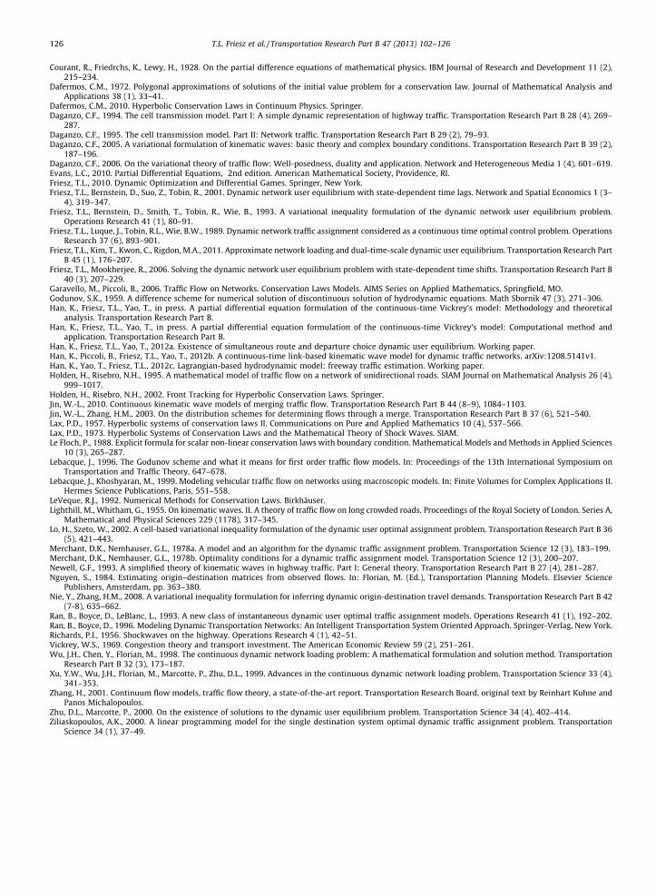
Courant, R., Friedrchs, K., Lewy, H., 1928. On the partial difference equations of mathematical physics. IBM Journal of Research and Development 11 (2),215–234.

Dafermos, C.M., 1972. Polygonal approximations of solutions of the initial value problem for a conservation law. Journal of Mathematical Analysis andApplications 38 (1), 33–41.

Dafermos, C.M., 2010. Hyperbolic Conservation Laws in Continuum Physics. Springer.Daganzo, C.F., 1994. The cell transmission model. Part I: A simple dynamic representation of highway traffic. Transportation Research Part B 28 (4), 269–

287.Daganzo, C.F., 1995. The cell transmission model. Part II: Network traffic. Transportation Research Part B 29 (2), 79–93.Daganzo, C.F., 2005. A variational formulation of kinematic waves: basic theory and complex boundary conditions. Transportation Research Part B 39 (2),

187–196.Daganzo, C.F., 2006. On the variational theory of traffic flow: Well-posedness, duality and application. Network and Heterogeneous Media 1 (4), 601–619.Evans, L.C., 2010. Partial Differential Equations, 2nd edition. American Mathematical Society, Providence, RI.Friesz, T.L., 2010. Dynamic Optimization and Differential Games. Springer, New York.Friesz, T.L., Bernstein, D., Suo, Z., Tobin, R., 2001. Dynamic network user equilibrium with state-dependent time lags. Network and Spatial Economics 1 (3–

4), 319–347.Friesz, T.L., Bernstein, D., Smith, T., Tobin, R., Wie, B., 1993. A variational inequality formulation of the dynamic network user equilibrium problem.

Operations Research 41 (1), 80–91.Friesz, T.L., Luque, J., Tobin, R.L., Wie, B.W., 1989. Dynamic network traffic assignment considered as a continuous time optimal control problem. Operations

Research 37 (6), 893–901.Friesz, T.L., Kim, T., Kwon, C., Rigdon, M.A., 2011. Approximate network loading and dual-time-scale dynamic user equilibrium. Transportation Research Part

B 45 (1), 176–207.Friesz, T.L., Mookherjee, R., 2006. Solving the dynamic network user equilibrium problem with state-dependent time shifts. Transportation Research Part B

40 (3), 207–229.Garavello, M., Piccoli, B., 2006. Traffic Flow on Networks. Conservation Laws Models. AIMS Series on Applied Mathematics, Springfield, MO.Godunov, S.K., 1959. A difference scheme for numerical solution of discontinuous solution of hydrodynamic equations. Math Sbornik 47 (3), 271–306.Han, K., Friesz, T.L., Yao, T., in press. A partial differential equation formulation of the continuous-time Vickrey’s model: Methodology and theoretical

analysis. Transportation Research Part B.Han, K., Friesz, T.L., Yao, T., in press. A partial differential equation formulation of the continuous-time Vickrey’s model: Computational method and

application. Transportation Research Part B.Han, K., Friesz, T.L., Yao, T., 2012a. Existence of simultaneous route and departure choice dynamic user equilibrium. Working paper.Han, K., Piccoli, B., Friesz, T.L., Yao, T., 2012b. A continuous-time link-based kinematic wave model for dynamic traffic networks. arXiv:1208.5141v1.Han, K., Yao, T., Friesz, T.L., 2012c. Lagrangian-based hydrodynamic model: freeway traffic estimation. Working paper.Holden, H., Risebro, N.H., 1995. A mathematical model of traffic flow on a network of unidirectional roads. SIAM Journal on Mathematical Analysis 26 (4),

999–1017.Holden, H., Risebro, N.H., 2002. Front Tracking for Hyperbolic Conservation Laws. Springer.Jin, W.-L., 2010. Continuous kinematic wave models of merging traffic flow. Transportation Research Part B 44 (8–9), 1084–1103.Jin, W.-L., Zhang, H.M., 2003. On the distribution schemes for determining flows through a merge. Transportation Research Part B 37 (6), 521–540.Lax, P.D., 1957. Hyperbolic systems of conservation laws II. Communications on Pure and Applied Mathematics 10 (4), 537–566.Lax, P.D., 1973. Hyperbolic Systems of Conservation Laws and the Mathematical Theory of Shock Waves. SIAM.Le Floch, P., 1988. Explicit formula for scalar non-linear conservation laws with boundary condition. Mathematical Models and Methods in Applied Sciences

10 (3), 265–287.Lebacque, J., 1996. The Godunov scheme and what it means for first order traffic flow models. In: Proceedings of the 13th International Symposium on

Transportation and Traffic Theory, 647–678.Lebacque, J., Khoshyaran, M., 1999. Modeling vehicular traffic flow on networks using macroscopic models. In: Finite Volumes for Complex Applications II.

Hermes Science Publications, Paris, 551–558.LeVeque, R.J., 1992. Numerical Methods for Conservation Laws. Birkhäuser.Lighthill, M., Whitham, G., 1955. On kinematic waves. II. A theory of traffic flow on long crowded roads. Proceedings of the Royal Society of London. Series A,

Mathematical and Physical Sciences 229 (1178), 317–345.Lo, H., Szeto, W., 2002. A cell-based variational inequality formulation of the dynamic user optimal assignment problem. Transportation Research Part B 36

(5), 421–443.Merchant, D.K., Nemhauser, G.L., 1978a. A model and an algorithm for the dynamic traffic assignment problem. Transportation Science 12 (3), 183–199.Merchant, D.K., Nemhauser, G.L., 1978b. Optimality conditions for a dynamic traffic assignment model. Transportation Science 12 (3), 200–207.Newell, G.F., 1993. A simplified theory of kinematic waves in highway traffic. Part I: General theory. Transportation Research Part B 27 (4), 281–287.Nguyen, S., 1984. Estimating origin–destination matrices from observed flows. In: Florian, M. (Ed.), Transportation Planning Models. Elsevier Science

Publishers, Amsterdam, pp. 363–380.Nie, Y., Zhang, H.M., 2008. A variational inequality formulation for inferring dynamic origin-destination travel demands. Transportation Research Part B 42

(7-8), 635–662.Ran, B., Boyce, D., LeBlanc, L., 1993. A new class of instantaneous dynamic user optimal traffic assignment models. Operations Research 41 (1), 192–202.Ran, B., Boyce, D., 1996. Modeling Dynamic Transportation Networks: An Intelligent Transportation System Oriented Approach. Springer-Verlag, New York.Richards, P.I., 1956. Shockwaves on the highway. Operations Research 4 (1), 42–51.Vickrey, W.S., 1969. Congestion theory and transport investment. The American Economic Review 59 (2), 251–261.Wu, J.H., Chen, Y., Florian, M., 1998. The continuous dynamic network loading problem: A mathematical formulation and solution method. Transportation

Research Part B 32 (3), 173–187.Xu, Y.W., Wu, J.H., Florian, M., Marcotte, P., Zhu, D.L., 1999. Advances in the continuous dynamic network loading problem. Transportation Science 33 (4),

341–353.Zhang, H., 2001. Continuum flow models, traffic flow theory, a state-of-the-art report. Transportation Research Board, original text by Reinhart Kuhne and

Panos Michalopoulos.Zhu, D.L., Marcotte, P., 2000. On the existence of solutions to the dynamic user equilibrium problem. Transportation Science 34 (4), 402–414.Ziliaskopoulos, A.K., 2000. A linear programming model for the single destination system optimal dynamic traffic assignment problem. Transportation

Science 34 (1), 37–49.


Dynamic user equilibrium based on a hydrodynamic model

Documents

Transcript of Dynamic user equilibrium based on a hydrodynamic model