This article was downloaded by: [University of Alberta]On: 28 January 2015, At: 07:37Publisher: Taylor & FrancisInforma Ltd Registered in England and Wales Registered Number: 1072954 Registered office: Mortimer House,37-41 Mortimer Street, London W1T 3JH, UK

Petroleum Science and TechnologyPublication details, including instructions for authors and subscription information:http://www.tandfonline.com/loi/lpet20

Experimental Testing of Interfacial Coupling in Two-Phase Flow in Porous MediaMuhammad Ayub a & Ramon G. Bentsen ba Petroleum Technology Research Centre, Faculty of Engineering, University of Regina ,Regina, Saskatchewan, Canadab School of Mining and Petroleum Engineering, University of Alberta , Edmonton, Alberta,CanadaPublished online: 14 Feb 2007.

To cite this article: Muhammad Ayub & Ramon G. Bentsen (2005) Experimental Testing of Interfacial Coupling in Two-PhaseFlow in Porous Media, Petroleum Science and Technology, 23:7-8, 863-897, DOI: 10.1081/LFT-200034457

To link to this article: http://dx.doi.org/10.1081/LFT-200034457

PLEASE SCROLL DOWN FOR ARTICLE

Taylor & Francis makes every effort to ensure the accuracy of all the information (the “Content”) containedin the publications on our platform. However, Taylor & Francis, our agents, and our licensors make norepresentations or warranties whatsoever as to the accuracy, completeness, or suitability for any purpose of theContent. Any opinions and views expressed in this publication are the opinions and views of the authors, andare not the views of or endorsed by Taylor & Francis. The accuracy of the Content should not be relied upon andshould be independently verified with primary sources of information. Taylor and Francis shall not be liable forany losses, actions, claims, proceedings, demands, costs, expenses, damages, and other liabilities whatsoeveror howsoever caused arising directly or indirectly in connection with, in relation to or arising out of the use ofthe Content.

This article may be used for research, teaching, and private study purposes. Any substantial or systematicreproduction, redistribution, reselling, loan, sub-licensing, systematic supply, or distribution in anyform to anyone is expressly forbidden. Terms & Conditions of access and use can be found at http://www.tandfonline.com/page/terms-and-conditions

PET #34457

Petroleum Science and Technology, 23:863–897, 2005Copyright © Taylor & Francis Inc.ISSN: 0161-2840 print/1096-4673 onlineDOI: 10.1081/LFT-200034457

Experimental Testing of Interfacial Coupling inTwo-Phase Flow in Porous Media

Muhammad AyubPetroleum Technology Research Centre, Faculty of Engineering,

University of Regina, Regina, Saskatchewan, Canada

Ramon G. BentsenSchool of Mining and Petroleum Engineering, University of Alberta,

Edmonton, Alberta, Canada

Abstract: Two-phase flow through natural porous media is affected by the interfacialcoupling that takes place across the interfaces located in a porous medium. Suchcoupling may be of two types: viscous and capillary. In this study, defining equationsfor the capillary and viscous coupling parameters have been constructed. Moreover,these equations, together with a modified form of Kalaydjian’s transport equations,have been used to analyze interfacial coupling in two-phase flow through porousmedia. On the basis of the analysis carried out, it is argued that interfacial couplinghas no effect on steady-state, cocurrent flow, and only a small effect on unsteady-state,cocurrent flow. Moreover, it is suggested that interfacial coupling has a significanteffect on steady-state, countercurrent flow. Two methods were used to test the theory.In the first method, data from steady-state, cocurrent, and countercurrent experimentswere used to show that experimentally determined values of the capillary couplingparameters were in good agreement with those predicted theoretically. Because ofexperimental problems, it was not possible to determine experimentally, when usingthe first method, the magnitude of the viscous coupling parameters. In the secondmethod, data from steady-state and unsteady-state, cocurrent flow experiments, usingfluids having different viscosity ratios, and porous media having different grain-sizedistributions, were used to test the theory. Because of a lack of sufficient precisionin the measured data, it was not possible to make definitive statements with respectto the adequacy of the theory, or the possible impact of viscosity ratio and grain-sizedistribution on capillary coupling. Moreover, for the same reason, it was not possibleto obtain reliable estimates of the magnitude of the capillary coupling parameters.Because the second method is based on the assumption that viscous coupling is

Received 1 January 2004; accepted 17 March 2004.Address correspondence to Muhammad Ayub, Petroleum Technology Research

Centre, Faculty of Engineering, University of Regina, Regina, Saskatchewan, Canada,S4S 0A2. E-mail: muhammad.ayub@uregina.ca

863

Dow

nloa

ded

by [

Uni

vers

ity o

f A

lber

ta]

at 0

7:37

28

Janu

ary

2015

864 M. Ayub and R. G. Bentsen

negligible, it was not possible to use this method to determine experimentally themagnitude of the viscous coupling parameters.

Keywords: capillarity, momentum transfer, interfacial coupling, capillary coupling,viscous coupling, two-phase flow, permeability coefficients, transport equations

INTRODUCTION

Conventionally, in immiscible, two-phase flow (oil and water) flow throughporous media problems, it is usual to ignore the effect of the interfacial cou-pling that takes place between the two flowing phases. However, on the basisof theoretical analysis, it has been known for a long time that interfacial cou-pling should be incorporated into immiscible, two-phase flow formulations(Ayub and Bentsen, 1999). Of interest here is not whether interfacial cou-pling exists, but rather, whether it is significant. In particular, is it necessary,when dealing with practical reservoir engineering problems, to use transportequations capable of accounting properly for interfacial coupling, or are theconventional transport equations adequate for dealing with such problems.

On the basis of experimental results presented in the literature (Lelièvre,1966; Bourbiaux and Kalaydjian, 1990; Bentsen and Manai, 1993; Bentsenand Manai, 1991), it appears that mobilities determined in a countercurrentflow experiment are less than those determined in the same sand-fluid sys-tem, in a cocurrent flow experiment. Such a result cannot be explained, ifone assumes that the conventional transport equations (Muskat, 1982) de-scribe correctly two-phase flow through porous media. That is, one mustresort to more sophisticated transport equations, such as those constructed byKalaydjian (1987), or others (de Gennes, 1983; de la Cruz and Spanos, 1983;Whitaker, 1986), to explain such a result.

In the conventional transport equations (Muskat, 1982), the flux is takento be proportional to one driving force, the potential gradient acting across agiven phase. In the more sophisticated transport equations, Muskat’s transportequation (Muskat, 1982) is modified to include a cross, or coupling, term thatis proportional to the potential gradient of the other phase. The need for such amodification is argued usually on the basis of symmetry, results arising out ofirreversible thermodynamics, or results obtained by using volume-averagingtechniques. Moreover, it is postulated usually that the coupling effect arisesbecause of the interfacial contact between the two phases flowing throughthe porous medium.

It is important to note that the transport equations proposed by dela Cruz and Spanos (1983), Whitaker (1986), and Kalaydjian (1987), al-though different in form, are equivalent. This is the case because the formof the transport equations being linear, the phenomenological coefficientsof any one of the sets of transport equations can be related algebraicallyto those for either of the other two sets of transport equations (Katchalsky

Dow

nloa

ded

by [

Uni

vers

ity o

f A

lber

ta]

at 0

7:37

28

Janu

ary

2015

Experimental Testing of Interfacial Coupling 865

and Curran, 1967). It is important to note also that, although the transportequations proposed by de la Cruz and Spanos (1983) and Whitaker (1986)have a firm theoretical foundation, those proposed by Kalaydjian (1987) donot. This is because Kalaydjian’s equations (Kalaydjian, 1987) are basedon the assumption that the nonequilibrium thermodynamics of a molecu-lar mixture can be used as a starting point to construct his transport equa-tions. This assumption is incorrect, because macroscopic thermodynamicsfor porous media differ from those that pertain at the pore scale (de la Cruzet al., 1993).

It has been usual to attribute interfacial coupling to the interfacial mo-mentum transfer that takes place in a porous medium (Ayub and Bentsen,1999). Such coupling is often referred to as viscous coupling. There existsalso the possibility that there might be an additional source of interfacialcoupling, namely, the coupling of pressures that takes place across the inter-faces located in a porous medium (Bentsen, 2001; Babchin and Yuan, 1997).Such coupling is referred to as capillary coupling (Bentsen, 2001). Note thateffects attributable to viscous coupling must be associated with the mobilitiesof the flowing phases, whereas effects attributable to capillary coupling mustbe associated with the potential gradients acting across the flowing phases.Because the flux of a given phase is proportional to both the mobility and thepotential gradient of that phase, it can be difficult to discern whether a giveninterfacial effect should be associated with the mobility or with the potentialgradient of the phase.

Countercurrent flows may be of two different types: unforced and forced(Bentsen, 2003). In unforced countercurrent flows, the magnitude of the po-tential gradients, the capillary pressure gradient, and/or the buoyancy forceper unit volume is small enough that capillary pressure can manifest itself inthe usual way. Consequently, in unforced countercurrent flow, the pressuregradients for both the wetting and the nonwetting phase have the same sign.In forced countercurrent flow, the magnitude of the driving forces is such thatcapillary pressure is unable to manifest itself in the usual way. In particular,in the steady-state, horizontal, forced, countercurrent flow experiments con-ducted by Bentsen and Manai (1993, 1991), it was determined experimentallythat the pressure gradients for the wetting and nonwetting phases, althoughconstant, acted in opposite directions. Consequently, it was not possible todetermine the capillary pressure for a given saturation, as is usually done,by measuring the difference in pressure between the two flowing phases at aparticular location along the length of the core.

Under flowing conditions, the difference in potential between two flow-ing phases may be slightly different from what would be the case under staticconditions (Bentsen and Manai, 1991; Bentsen, 1998). That is to say, hydro-dynamic effects may modify slightly the difference in potential between thetwo flowing phases (Bentsen, 1998). It has been found experimentally that,during both cocurrent and countercurrent flow, the effect of such hydrody-namic forces is to modify slightly the magnitude of the nonwetting potential

Dow

nloa

ded

by [

Uni

vers

ity o

f A

lber

ta]

at 0

7:37

28

Janu

ary

2015

866 M. Ayub and R. G. Bentsen

gradient (Bentsen, 1992). As a consequence, in horizontal, steady-state, cocur-rent flow, for example, the two straight lines representing the distribution ofpressure in the two flowing phases are almost, but not exactly parallel, asthey are usually taken to be (Bentsen and Manai, 1993).

To help differentiate between viscous and capillary coupling effects, itis desirable to have defining equations for both the viscous coupling and thecapillary coupling parameters. Thus, the first objective of this study is toconstruct defining equations for the capillary and viscous coupling parame-ters. The second objective is to use these equations, together with modifiedforms (Bentsen, 2001) of the transport equations proposed by Kalaydjian(1987), to determine the effect of interfacial coupling on horizontal, two-phase flow through natural porous media. The final objective of the studyis to test experimentally the theory of interfacial coupling by using data ac-quired in steady-state, cocurrent, and countercurrent flow experiments and inunsteady-state, cocurrent flow experiments.

THEORY

The following analysis is confined to the stable, collinear, horizontal flowof two immiscible, incompressible fluids through a water-wet, isotropic, andhomogeneous porous medium where Phase 1 is the wetting phase and Phase 2is the nonwetting phase.

Basic Equations

Any self-consistent system of equations that may be used to describe two-phase flow through porous media must include two transport equations. Anyof the transport equations discussed earlier (Kalaydjian, 1987; de la Cruz andSpanos, 1983; Whitaker, 1986) may be used for this purpose. However, be-cause the phenomenological coefficients associated with both Muskat’s trans-port equations (Muskat, 1982) and those of Kalaydjian (1987) are generalizedconductances or mobilities, it is more convenient, in this study, to use thetransport equations proposed by Kalaydjian (1987). Keeping in mind the as-sumptions made above, these equations may be written as:

v1 = −λ11∂p1

∂x− λ12

∂p2

∂x(1)

and

v2 = −λ21∂p1

∂x− λ22

∂p2

∂x(2)

where λij = kij /µi ; i, j = 1, 2. By considering the horizontal, steady-state,cocurrent and countercurrent flow of two immiscible fluids through a porous

Dow

nloa

ded

by [

Uni

vers

ity o

f A

lber

ta]

at 0

7:37

28

Janu

ary

2015

Experimental Testing of Interfacial Coupling 867

medium, it can be demonstrated (Bensten, 2001) that the λij , i, j = 1, 2 aredefined by:

λ11 =(

1 + α1

2

)λ◦

1 (3)

λ12

R12=

(1 − α1

2

)λ◦

1 (4)

R12λ21 =(

1 − α2

2

)λ◦

2 (5)

and

λ22 =(

1 + α2

2

)λ◦

2 (6)

where the αi , i = 1, 2 are the interfacial coupling parameters; the λ◦i = k◦

i /µi ,i = 1, 2 are the conventional mobilities determined in a horizontal, steady-state, cocurrent flow experiment; and R12 is a weak function of normalizedsaturation that has been introduced to allow for the possibility that hydro-dynamic effects (Bentsen, 1998) may have an influence on the difference inpressure between the two flowing phases.

If Eqs. (3) and (4) are introduced into Eq. (1), and Eqs. (5) and (6) intoEq. (2), one obtains:

v1 = −λ◦1

[1

2(1 + α1)

∂p1

∂x+ R12

2(1 − α1)

∂p2

∂x

](7)

and

v2 = −λ◦2

[1

2R12(1 − α2)

∂p1

∂x+ 1

2(1 + α2)

∂p2

∂x

](8)

To complete the system of equations needed to describe two-phase flow,a relationship between the macroscopic pressure difference between the twoflowing phases and saturation is needed. Usually, a macroscopic capillarypressure equation (Kalaydjian, 1987; de la Cruz and Spanos, 1983; Whitaker,1986) is used for this purpose. However, such equations are simply a zerothorder constraint and not the dynamic relationship between the macroscopicpressure difference and saturation that is needed to describe properly thechanges in saturation that occur during two-phase flow in porous media.Recently, de la Cruz et al. (1995) demonstrated that a process-dependentequation that constrains the macroscopic capillary pressure, together with theequations of motion and the continuity equations form a complete system of

Dow

nloa

ded

by [

Uni

vers

ity o

f A

lber

ta]

at 0

7:37

28

Janu

ary

2015

868 M. Ayub and R. G. Bentsen

system of equations for describing the immiscible flow of two incompress-ible fluids through porous media. Because the process-dependent equationcontains a parameter of unknown composition and because it has yet to betested experimentally, this new equation is not used in this study. Rather, aslightly modified form of the macroscopic capillary pressure equation is usedinstead.

Under flowing conditions, the difference in pressure between two flowingphases may be slightly different from what would be the case under staticconditions (Bentsen and Manai, 1991; Bentsen, 1998). This can be accountedfor by modifying slightly the magnitude of the nonwetting phase-pressuregradient (Bentsen, 1992, 1998, 1994). By accounting for such hydrodynamiceffects (Bentsen, 1994), Bentsen (1992, 1998, 1994) has established, for alltypes of horizontal, one-dimensional flow, that:

∂Pc

∂x= R12

∂p2

∂x− ∂p1

∂x(9)

By introducing Eq. (9) into Eqs. (7) and (8), it may be shown that:

v1 = −λ◦1

(∂p1

∂x+ 1 − α1

2

∂Pc

∂x

)(10)

and

v2 = −λ◦2

(∂p2

∂x− 1 − α2

2R12

∂Pc

∂x

)(11)

Interfacial Coupling

Consider now a horizontal, steady-state, countercurrent flow experiment. Forsuch an experiment, one may, by using conventional theory, write:

vi = −λ∗i

∂pi

∂x, i = 1, 2 (12)

where the λ∗i = k∗

i /µi , i = 1, 2 are the conventional mobilities measured in ahorizontal, steady-state, countercurrent flow experiment. On the basis of theexperimental results presented by Bentsen and Manai (1993, 1991), it can beinferred that (Bentsen, 1998):

λ∗i = αiλ

◦i , i = 1, 2 (13)

Introducing Eq. (13) into Eq. (12) yields:

vi = −αiλ◦i

∂pi

∂x, i = 1, 2 (14)

Dow

nloa

ded

by [

Uni

vers

ity o

f A

lber

ta]

at 0

7:37

28

Janu

ary

2015

Experimental Testing of Interfacial Coupling 869

The defining equations for the interfacial coupling parameters dependon the nature of the interfacial coupling that takes place across the inter-faces located in a porous medium. Two types of interfacial coupling can takeplace: viscous and capillary (Bentsen, 2001; Babchin and Yuan, 1997). If aninterfacial coupling effect is due to viscous coupling, it should be associatedwith the appropriate mobility. If, however, the interfacial coupling effect isdue to the capillarity of the porous medium, it should be associated with theappropriate pressure gradient. Such a separation of the interfacial couplingeffects can be achieved by defining αi , i = 1, 2 as follows:

αi = αviαci (15)

where the αvi , i = 1, 2 are the viscous coupling parameters, and the αci ,i = 1, 2 are the capillary coupling parameters. Upon introducing Eq. (15)into Eq. (14), one obtains:

vi = −αviλ◦i αci

∂pi

∂x, i = 1, 2 (16)

Viscous Coupling

When interfacial coupling arises because of interfacial momentum transfer,it must be associated with the mobilities, λ12 and λ21 (Bentsen, 2001). Inanalogous models of porous media (Bacri et al., 1990; Rose, 1990), suchcross parameters are equal. Thus, for the purposes of constructing the viscouscoupling parameters only, it is supposed that:

λ12 = λ21 (17)

Note that, as can be seen in Basic Equations, making this supposition doesnot result in the cross mobilities appearing in Eqs. (1) and (2) being equal.Rather, it only results in the shape of the traditional mobilities, λ◦

1 and λ◦2,

being influenced by viscous coupling.Equation (17) may be used to construct defining equations for the viscous

coupling parameters, αv1 and αv2. In particular, if αv1 is defined by:

αv1 = 1 − C

R12

λ◦2

λ◦w

(18)

and, if αv2 is defined by:

αv2 = 1 − CR12λ◦

1

λ◦w

(19)

it follows, in view of Eqs. (4) and (5), modified so that only viscous couplingis being considered (αc1 = αc2 = 1), that:

λ12 = λ21 = C

2

λ◦1λ

◦2

λ◦w

(20)

Dow

nloa

ded

by [

Uni

vers

ity o

f A

lber

ta]

at 0

7:37

28

Janu

ary

2015

870 M. Ayub and R. G. Bentsen

where C is a parameter that controls the amount of viscous coupling thatis taking place, and where λ◦

w is a weighted mobility introduced to ensuredimensional consistency. For the sake of internal consistency, it is necessarythat λ◦

w = λ◦1r when the normalized saturation, S, equals 1 and that λ◦

w = λ◦2r

when S equals 0, where the λ◦ir , i = 1, 2 are the endpoint mobilities for the

wetting and nonwetting phase, respectively. A simple equation for λ◦w that

meets this requirement is:

λ◦w = Sλ◦

1r + (1 − S)λ◦2r (21)

Given the validity of Eqs. (16), (19), and (21), it may be shown that:

αv1 = 1 − C

R12

kr2

1 + (M − 1)S(22)

and that:

αv2 = 1 − CR12Mkr1

1 + (M − 1)S(23)

where the kri , i = 1, 2 are the normalized relative permeabilities to thewetting and nonwetting phases, respectively, and where:

M = λ◦1r

λ◦2r

= k◦1r

µ1

µ2

k◦2r

(24)

is the endpoint mobility ratio.Zarcone and Lenormand (1994), on the basis of experimental evidence,

and Rakotomalala et al. (1995), on the basis of theoretical analysis, suggestthat the fraction of the total flux that is due to viscous coupling duringhorizontal flow is insignificant (of order 10−2 or less). If such is the case,interfacial momentum transfer cannot be used to explain the experimentalobservation (Lelièvre, 1966; Bentsen and Manai, 1991; 1993) that, for a givenpotential gradient, the total flux in a steady-state, countercurrent experiment issignificantly less than that in a steady-state, cocurrent flow experiment. Thatis, if such a result is to be explained, a different kind of interfacial couplingmust be postulated. One possibility is to suppose that interfacial couplingtakes place because of the capillarity of the porous medium (Bentsen, 2001).This possibility is explored in the next section.

Capillary Coupling

Because of the capillarity of porous media, there exists a difference in pres-sure, the capillary pressure, across the interfaces located in porous media.

Dow

nloa

ded

by [

Uni

vers

ity o

f A

lber

ta]

at 0

7:37

28

Janu

ary

2015

Experimental Testing of Interfacial Coupling 871

Interfacial coupling that arises out of the coupling of macroscopic pressuresacross such interfaces is referred to as capillary coupling (Bentsen, 2001).Some insight into the nature of such coupling can be gained, provided chan-nel flow (Chatenever and Calhoun, 1952; Rapoport and Leas, 1953) theory isaccepted. In channel flow theory, it is postulated that the channels in whicha specific fluid is flowing are bounded in part by fluid-solid surfaces and inpart by fluid-fluid interfaces.

Geometrical Model of Channel Flow. For the purposes of constructinga defining equation for the capillary coupling parameter only, it is supposedthat the wetting phase and the nonwetting phase are flowing through twocontiguous, partially overlapping channels (Figure 1). The wetting fluid isflowing, from left to right, in the channel located on the left side of thefigure, and the nonwetting phase is flowing in the same direction in thechannel located on the right side of the figure. In the middle of the figure,the two channels overlap, with the wetting phase flowing through the upperpart of the section, and the nonwetting fluid flowing through the lower part ofthe section. To keep the analysis simple, it is supposed that channels having

Figure 1. An idealized schematic of the representative macroscopic surface (RMS),one located in a Phase 1 channel, and one located in a Phase 2 channel.

Dow

nloa

ded

by [

Uni

vers

ity o

f A

lber

ta]

at 0

7:37

28

Janu

ary

2015

872 M. Ayub and R. G. Bentsen

simple geometry may be used to model the flow of the two fluids and thatthe walls of the channels have zero thickness.

A vertical plane, which is oriented parallel to the direction of flow, isintroduced at the end of the overlapping part of the channel in which non-wetting fluid is flowing. Similarly, a second plane, which is parallel to thefirst, is introduced at the end of the overlapping part of the channel in whichwetting fluid is flowing. The first plane is located in such a way that theupper part of the plane, when viewed from within the channel flowing wet-ting fluid, contains Phase 1-Phase 2 interfaces, whereas the lower part ofthe plane contains Phase 1-Phase 1 interfaces. The upper part of the secondplane, when viewed from within the channel flowing nonwetting fluid, con-tains Phase 2-Phase 2 interfaces, whereas the lower part of the plane containsPhase 2-Phase 1 interfaces.

To determine the effect of interfacial coupling on the pressures of thefluids flowing in the two channels, the pressures of the two fluids are av-eraged over the area of the introduced planes. The extent of the area overwhich the pressures are averaged is assumed to be larger than a representa-tive elementary surface (RES), so that macroscopic pressures may be used inthe analysis that follows. Moreover, the area over which the averaging takesplace is assumed to be smaller than the cross-sectional area of the walls ofthe channels in which the fluids are flowing. The surface over which the areaaveraging is carried out is referred to as a representative macroscopic surface(RMS). Two highly idealized versions of such surfaces, the first located inthe wall of a channel flowing wetting fluid, and the second located in thewall of a channel flowing nonwetting fluid, are depicted in Figure 1. Notethat, for reasons of clarity, Figure 1 is not drawn to scale.

Estimation of Average Pressure Gradients. To estimate the average pres-sure for Phase 1, it is supposed that:

F1S = Ab(1 − φ)p1 (25)

F11 = Abφc11p1 (26)

and

F12 = Abφc12p1 (27)

where F1S is the force acting orthogonally on the fluid 1-solid part of thefirst RMS and where F11 and F12 are the forces acting orthogonally on thePhase 1-Phase 1 and Phase 1-Phase 2 portions of the fluid-fluid portion of theRMS, respectively. The bulk area of the RMS is defined by Ab, the porosityby φ, and c11 and c12 are the fractions, on the Phase 1 side, of the fluid-fluidinterface that are Phase 1-Phase 1 and Phase 1-Phase 2 interface, respectively.The phase pressures, p1 and p2, are assumed to be measured at the midpoint

Dow

nloa

ded

by [

Uni

vers

ity o

f A

lber

ta]

at 0

7:37

28

Janu

ary

2015

Experimental Testing of Interfacial Coupling 873

of the RMS. Under conditions of steady-state flow, Eq. (9) may be integratedto show that the pressure drop across the Phase 1-Phase 2 portion of thefluid-fluid interface may be defined by:

R12p2 − p1 = Pc (28)

Solving Eq. (28) for p1 and introducing the result into Eq. (27), there results:

F12 = Abφc12(R12p2 − Pc) (29)

By summing the forces defined by Eqs. (25), (26), and (29) and by dividingby Ab, the average pressure of the wetting phase, acting at the midpoint ofthe first RMS, may be shown to be:

p1 = [1 − (1 − c11)φ]p1 + c12φ(R12p2 − Pc) (30)

In view of the fact that:

Abφc11 + Abφc12 = Abφ

it follows that:

c11 + c12 = 1 (31)

The introduction of Eq. (31) into Eq. (30) yields:

p1 = (1 − c12φ)p1 + c12φ(R12p2 − Pc) (32)

Consider next the contiguous and partially overlapping channel flowing,under steady-state conditions, Phase 2, the nonwetting phase (Figure 1). Ananalysis similar to that presented above for Phase 1 may be used to demon-strate that the average pressure of the nonwetting phase, acting at the midpointof the second RMS, is defined by:

p2 = (1 − c21φ)p2 + c21φ

R12(p1 + Pc) (33)

where

c21 + c22 = 1 (34)

and where c21 and c22 define the fractions, on the Phase 2 side, of thefluid-fluid interface that are Phase 2-Phase 1 interface and Phase 2-Phase 2interface, respectively.

Dow

nloa

ded

by [

Uni

vers

ity o

f A

lber

ta]

at 0

7:37

28

Janu

ary

2015

874 M. Ayub and R. G. Bentsen

Taking the partial derivatives of Eqs. (32) and (33) with respect to thedirection of flow, x, and keeping in mind that at steady-state ∂Pc/∂x = 0,yields:

∂p1

∂x= (1 − c12φ)

∂p1

∂x+ c12R12φ

∂p2

∂x(35)

and

∂p2

∂x= c21φ

R12

∂p1

∂x+ (1 − c21φ)

∂p2

∂x(36)

For steady-state, cocurrent flow [see Eq. (9)], R12∂p2/∂x = ∂p1/∂x.Introducing this result into Eqs. (35) and (36) leads to:

∂p1

∂x= ∂p1

∂x(37)

and

∂p2

∂x= ∂p2

∂x(38)

Thus, as expected, it can be inferred from Eqs. (37) and (38) that, for cocur-rent, steady-state flow, the average (or effective) driving force for a givenphase is the appropriate pressure gradient for that phase. This is the casebecause, for cocurrent flow, the capillary coupling effects are equal in mag-nitude and opposite in sign; hence, they cancel out. That is to say, becauseboth driving forces are acting in the same direction, the coupling of pres-sures across the interfaces located in the porous medium has no effect on themagnitude of the two pressure gradients. This is consistent with conventionalwisdom and with the results presented in an earlier paper (Bentsen, 2001).

For steady-state, forced, countercurrent flow, the pressure gradients areopposite in sign; that is, R12∂p2/∂x = −∂p1/∂x. If this result is introducedinto Eqs. (35) and (36), it follows that:

∂p1

∂x= (1 − 2c12φ)

∂p1

∂x(39)

and

∂p2

∂x= (1 − 2c21φ)

∂p2

∂x(40)

Hence, on the basis of Eq. (39), it appears that for steady-state, forced,countercurrent, flow, the average (or effective) driving force for the wettingphase is smaller, by the factor (1−2c12φ), than the measured pressure gradi-ent for the wetting phase. Similarly, on the basis of Eq. (40), it appears thatthe average (or effective) driving force for the nonwetting phase is smaller, by

Dow

nloa

ded

by [

Uni

vers

ity o

f A

lber

ta]

at 0

7:37

28

Janu

ary

2015

Experimental Testing of Interfacial Coupling 875

the factor (1−2c21φ), than the measured pressure gradient in the nonwettingphase. The reason for this is that the wetting and nonwetting pressure gradi-ents are acting in opposite directions. In particular, for countercurrent flow,the capillary coupling effects, although equal in magnitude, have the samesign, because the pressure gradients are opposite in sign. Consequently, forcountercurrent flow, the average (or effective) driving forces per unit volumeare less than the measured phase pressure gradients. That is to say, becausethe driving forces for the two fluids are acting in opposite directions, thecoupling of pressures across the interfaces located in the porous medium hasthe effect of reducing the magnitude of the two pressure gradients.

Construction of Equations for Capillary Coupling Parameters

In view of Eq. (16), and Eqs. (39) and (40), it appears that the capillarycoupling parameters, αc1 and αc2, may be defined, respectively, by:

αc1 = 1 − 2c12φ (41)

and

αc2 = 1 − 2c21φ (42)

Two more equations are needed to define completely the cij , i, j =1, 2 parameters. To obtain these equations, two compatibility conditions areimposed. To be consistent, the area of the Phase 1-Phase 2 interface on thewetting side of the first RMS should equal the area of the Phase 2-Phase 1interface on the nonwetting side of the second RMS. This can be achievedby setting:

c12 = c21 (43)

At steady state, there should be no local saturation gradients in the trans-verse direction to flow. For this to be the case, it is necessary that:

c11 = c21 (44)

Eqs. (31), (34), (43), and (44) comprise a system of four equations in fourunknowns, the cij , i, j = 1, 2, which may be solved to show that:

c11 = c12 = c21 = c22 = 0.5 (45)

Note that the cij , i, j = 1, 2 should not be viewed as saturations inasmuchas saturation is dictated by the relative number of channels, and their cross-sectional area (orthogonal to the direction of flow), which are transportingPhase 1 and Phase 2, respectively.

Dow

nloa

ded

by [

Uni

vers

ity o

f A

lber

ta]

at 0

7:37

28

Janu

ary

2015

876 M. Ayub and R. G. Bentsen

On introducing Eq. (45) into Eqs. (41) and (42), it follows, in view ofEq. (44), that:

αc1 = αc2 = αc = 1 − φ (46)

a result that is consistent with the results presented in an earlier article(Bentsen, 2001).

In constructing Eq. (46), the defining equation for α = αc, the porosity,φ, was assumed to be that in a plane parallel to the direction of flow. Forthe isotropic, homogeneous, natural porous media being considered here, theporosity of a plane is independent of the direction of the plane. Hence, inview of Eq. (46), 0 < α < 1. That is, in isotropic, homogeneous, naturalporous media, α cannot take on the limiting values of 0 and 1, because, forsuch values, the porous medium ceases to exist.

EXPERIMENTAL TESTING

To obtain values for the four generalized permeability coefficients [Eqs. (1)and (2)], and from them values for the interfacial coupling parameters, onemust conduct at least two types of experiments (Rose, 1988). Over the years,various combinations of experiments have been proposed to quantify thegeneralized permeability coefficients. Rose (1988) suggested conducting twotypes of experiments (i.e., horizontal flow and vertical flow experiments) toobtain the required parameters. However, the implementation of this schemeis difficult because of problems associated with the accurate measurement ofgravitational effects and the difference in the vertical and horizontal veloc-ities. In their experimental research, Manai (1991) and Bentsen and Manai(1993, 1991) presented a scheme involving cocurrent flow and countercur-rent flow to overcome the difficulties associated with Rose’s approach, whichused horizontal and vertical flows (Rose, 1988). Goode (1991) suggestedindirect measurement methods involving two types of experiments. Liangand Lorenz (1994) and Liang (1993) proposed a combination of steady-stateand unsteady-state experiments, once again overcoming the above mentioneddifficulties of Rose’s method.

In another study, Dullien and Dong (1996) presented an experimental ap-proach for determining the four generalized permeability coefficients, whichinvolved setting the pressure gradient in one of the two flowing phases equalto zero. The values of the cross coefficients were found to differ significantlyfrom the values of the effective permeability to water and oil. However, theirapproach of using one flowing fluid, while keeping the other stationary, is alimiting case of two-phase flow phenomena; that is, it does not represent theoverall mechanism of two-phase flow through a porous system. Moreover,they were unable to determine the net contribution of viscous coupling to theflow of water and oil, when the respective pressure gradients across the wateror oil phase were set equal to 0.

Dow

nloa

ded

by [

Uni

vers

ity o

f A

lber

ta]

at 0

7:37

28

Janu

ary

2015

Experimental Testing of Interfacial Coupling 877

In this study, two methods were used to obtain values for the interfacialcoupling parameters. In the first method, called the steady-state method, twosteady-state experiments, one a cocurrent flow (SSCO) and one a counter-current flow (SSCT) experiment, were used. In the second method, calledthe unsteady-state method, two cocurrent experiments, one a steady-stateexperiment and one an unsteady-state (USCO) experiment, were used. Toimplement the steady-state method, the steady-state flow experiments carriedout by Manai (1991) in water-wet, unconsolidated sand packs were used.Two sets of runs were conducted by Manai (1991), the second being a repli-cate of the first. A description of the experimental materials, equipment, andprocedures used by Manai (1991) is available in the literature (Bentsen andManai, 1993, 1991). Although there are differences in the fluids used and inhow the pressures and saturations were measured, the experimental materials,equipment, and procedures used by Manai (1991) were essentially similar tothose described below which were used by Ayub (2000).

Ayub (2000) carried out the steady-state and unsteady-state, cocurrentflow experiments used to implement the unsteady-state method. He performedthree sets of SSCO and USCO flow experiments in which two types of porousmedia and two different viscosity fluids were used. Note that an experimentalset comprises two types of two-phase flow experiments: SSCO and USCOexperiments using the same core and the same fluids for both runs. Table 1provides the average sand and fluid properties used to conduct the two-phaseSSCO and USCO flow experiments.

The schematic diagram of the core flooding experimental system used byAyub (2000) to conduct the two-phase flow experiments is shown in Figure 2.

Table 1. Average sandpack and fluid properties at room temperature

Properties Set 1 Set 2 Set 3

Grain size, mesh, µm 80–120 80–120 100–170(180–125) (180–125) (150–90)

Bulk volume, cc 401.00 401.00 401.00Pore volume, cc 148.37 149.57 130.33Porosity, fraction 0.370 0.373 0.325Absolute permeability to water, darcy 17.88 19.30 1.70Irreducible water saturation, fraction 0.11 0.12 0.16Irreducible oil saturation, fraction 0.09 0.10 0.12Water viscosity, mPa.s 1.00 1.00 1.00Water density, gm/cc 0.99 0.99 0.99Oil viscosity, mPa.s 1.69 15.00 1.69Oil density, gm/cc 0.77 0.83 0.77Interfacial tension, dyne/cm 32.00 45.00 32.00Capillary number 0.35 0.21 0.02Mobility ratio 1.44 5.29 1.86

Dow

nloa

ded

by [

Uni

vers

ity o

f A

lber

ta]

at 0

7:37

28

Janu

ary

2015

Fig

ure

2.E

xper

imen

tal

setu

pfo

rSS

CO

and

USC

Otw

o-ph

ase

flow

.

878

Dow

nloa

ded

by [

Uni

vers

ity o

f A

lber

ta]

at 0

7:37

28

Janu

ary

2015

Experimental Testing of Interfacial Coupling 879

This experimental setup is similar to the one used by Chang (1996). Amongothers, the main differences between the current system and that used byChang (1996) include the saturation measurement system (Ayub and Bentsen,2000) and the core-holder. For the sake of brevity, the complete experimentalsystem is not described here. The reader interested in a complete descrip-tion of the experimental apparatus is referred to Ayub (2000) and Ayub andBentsen (2000, 2001). Here attention is focused mainly on describing thetypical results obtained during the overall experimental investigation to testthe new theory of interfacial coupling (capillary coupling).

During the data analysis for each set of experiments, attention wasfocussed on testing the theory pertaining to the physical origin of interfa-cial coupling [Eqs. (10) and (11)]. Specifically, attempts were made to testEqs. (10) and (11) with the help of measured and calculated experimentaldata. Capillary pressure and mobility curves, for both phases, were obtainedfrom the SSCO runs, whereas phase velocities and the saturation gradientsneeded to construct the capillary pressure gradients were determined from thedata taken in the USCO runs. Further details are available in Ayub (2000).

Steady-State Method

To determine with steady-state data, the parameters αci and αvi , i = 1, 2, itis necessary to find a relationship between λ∗

i and λ◦i , i = 1, 2. This can be

achieved by using Eqs. (12) and (17). In particular, if these two equationsare equated, it follows that:

λ∗i = αciαviλ

◦i , i = 1, 2 (47)

By introducing into Eq. (47) the definitions for mobility and normalizedrelative permeability, it may be shown that:

k∗ir k

∗ri = αcik

◦irαvik

◦ri , i = 1, 2 (48)

Based on a comparison of cocurrent and countercurrent conventional effectivepermeabilities (Bensten, 1998), it may be inferred that:

k∗ir = αcik

◦ir , i = 1, 2 (49)

Introducing Eq. (49) into Eq. (48) yields:

k∗ri = αvik

◦ri , i = 1, 2 (50)

Given the validity of the above analysis, it appears that the magni-tude of the k∗

ir , i = 1, 2, is dictated by [see Eq. (49)] the capillary cou-pling parameters, αci , i = 1, 2. Moreover, the shape of the k∗

ri , i = 1, 2,

Dow

nloa

ded

by [

Uni

vers

ity o

f A

lber

ta]

at 0

7:37

28

Janu

ary

2015

880 M. Ayub and R. G. Bentsen

is influenced by [see Eq. (50)] the viscous coupling parameters, αvi , i = 1, 2.Note that the effect of the αvi , i = 1, 2 [see Eqs. (22) and (23)], is to causethe magnitude of the k∗

ri , i = 1, 2, to be less than that of the k◦ri , i = 1, 2

in the open interval 0 < S < 1. However, if the amount of viscous couplingis insignificant (of order 10−2), the k∗

ri should, for all practical purposes, beidentical to the k◦

ri , i = 1, 2, provided no other factors are involved.

Experimental Testing of the Steady-State Method

The steady-state method for estimating αci , i = 1, 2, can be implementedby comparing [see Eq. (49)] cocurrent effective permeabilities (or relativepermeabilities) with countercurrent effective permeabilities (or relative per-meabilities). A set of such relative permeabilities, measured by Manai (1991),is depicted in Figure 3. By using the polynomials used to fit the rela-tive permeability data presented in Figure 3, the ratio of the countercurrentto cocurrent endpoint, wetting-phase relative permeabilities was estimatedto be about 0.639, whereas that for the nonwetting-phase relative perme-abilities was estimated to be about 0.642. Based on a porosity value of0.358, the theoretical value of αc1 = αc2 = αc can be estimated to be[see Eq. (46)] 0.642. Manai (1991) also measured a replicate set of rel-ative permeabilities (not reported here). By using a similar approach, theratio of the countercurrent to cocurrent endpoint, wetting-phase replicate rel-ative permeabilities was estimated to be about 0.646, whereas that for thenonwetting-phase, replicate relative permeabilities was estimated to be about0.644. Based on a porosity of 0.354 for the porous medium used to determine

Figure 3. Comparison of steady-state cocurrent and countercurrent relative perme-abilities.

Dow

nloa

ded

by [

Uni

vers

ity o

f A

lber

ta]

at 0

7:37

28

Janu

ary

2015

Experimental Testing of Interfacial Coupling 881

the replicate relative permeabilities, αc can be estimated, by using Eq. (46),to be 0.646. Thus, when using the data taken by Manai (1991), there is goodagreement between experimentally determined and theoretically predictedvalues of αc.

As can be seen from Eq. (50), an estimate of αvi , i = 1, 2, can be madeby comparing the normalized relative permeabilities measured in a cocurrentexperiment with those measured in a countercurrent experiment, provided noother effects come into play. Such a comparison, for the relative permeabili-ties depicted in Figure 3, is shown in Figure 4. Note that the countercurrent,normalized relative permeability curves for both the wetting and the non-wetting phase fall above those for cocurrent flow, contrary to what mightbe expected if only viscous coupling had a significant role to play in thedisplacements used to measure the relative permeabilities. This was also thecase for the replicate set of normalized relative permeabilities. In an effortto explain this behavior, the relative permeabilities, for both cocurrent andcountercurrent flow, depicted in Figure 4, were compared with those deter-mined in the replicate set of experiments. Similar differences to those seenin Figure 4 were observed between a given type of curve (say the cocurrent,wetting-phase curve) measured in the original set of experiments and thatmeasured in the replicate set of experiments. A countercurrent displacementcan be viewed as a kind of replicate displacement, albeit one in which thetwo phases are flowing in opposite directions. Hence, a possible explanationfor the difference between the cocurrent and countercurrent curves observedin Figure 4 is that the countercurrent curves were obtained by using replicateexperiments. Zarcone and Lenormand (1994) and Rakotomalala et al. (1995)suggest that the viscous coupling effect is small (of order 10−2). If such is

Figure 4. Comparison of steady-state cocurrent and countercurrent normalizedrelative permeabilities.

Dow

nloa

ded

by [

Uni

vers

ity o

f A

lber

ta]

at 0

7:37

28

Janu

ary

2015

882 M. Ayub and R. G. Bentsen

the case, it is expected that differences arising out of the use of replicateexperiments to estimate the countercurrent curves would mask completelyany viscous coupling effects. As a consequence, Figure 4 cannot be used asa basis for estimating the magnitude of the αvi , i = 1, 2.

Unsteady-State Methods

In Eq. (15) αci and αvi , i = 1, 2 appear as a product. This makes it im-possible, when using unsteady-state data, to distinguish between capillaryand viscous coupling. Consequently, because it has been suggested that theviscous coupling effect is negligibly small (Zarcone and Lenormand, 1994;Rakotomalala et al., 1995), it is assumed in the analysis which follows thatthe αvi , i = 1, 2 are equal to one. Hence, in view of Eq. (15), αi =αci , i = 1, 2. Keeping this in mind, the introduction of Eq. (41) intoEq. (10), and the introduction of Eq. (42) into Eq. (11), yields, after somerearrangement,

− v1

λ◦1

= ∂p1

∂x+ c12φ

∂Pc

∂x(51)

and

− v2

λ◦2

= ∂p2

∂x− c21φ

∂Pc

∂x(52)

where, in Eq. (52), R12 has been set equal to 1. This was done for two reasons.First, because of observed inconsistencies in the phase pressure gradients, itwas not possible to use the relation R12 = 1 − a(1 − S) (Bentsen, 1992)to determine the experimental values of a (Ayub, 2000). Second, becausethe experiments involved only cocurrent flow, this simplification should notintroduce any significant amount of error into the analysis (Bentsen, 1998,1994). Setting R12 = 1 resulted in the pressure gradients along the length ofthe core for both the wetting and the nonwetting phase during all SSCO runsbeing set equal to each other.

The parameters c12 and c21 are the fractions of the fluid-fluid interfaceof an RMS that are fluid 1-fluid 2 interface and fluid 2-fluid 1 interface,respectively. Theoretically [see Eq. (45)], c12 = c21 = 0.5. Moreover, becausec12 and c21 are fractions, it follows that 0 ≤ c12 ≤ 1 and that 0 ≤ c21 ≤ 1.

Two approaches were used to test the unsteady-state theory. In the firstapproach, an attempt was made to determine experimentally the magnitudeof c12 and c21. In the second approach, various values of c12 and c21 wereassumed, thus enabling the calculation of the pressure profiles, and then thecalculated pressure profiles were compared with the experimentally measuredpressure profiles.

Dow

nloa

ded

by [

Uni

vers

ity o

f A

lber

ta]

at 0

7:37

28

Janu

ary

2015

Experimental Testing of Interfacial Coupling 883

First Approach

Solving Eqs. (51) and (52) for c12 and c21, one obtains, respectively,

c12 =v1

λ◦1

+ ∂p1

∂x

φ∂Pc

∂x

(53)

and

c21 =v2

λ◦2

+ ∂p2

∂x

φ∂Pc

∂x

(54)

To use this method for testing the theory, measured and calculated data fromthe USCO and SSCO runs were used to calculate the right-hand side (RHS)of Eqs. (53) and (54). In particular, v1, v2, ∂p1/∂x, ∂p2/∂x, and ∂Pc/∂x

were determined from the data taken in the USCO runs, whereas λ◦1 and

λ◦2 were determined from the data taken in the SSCO runs. If the theory

underlying Eqs. (53) and (54) is valid, the calculations performed to determinethe magnitude of c12 and c21 should lead [in light of Eq. (45)] to values forc12 and c21 in the vicinity of 0.5.

Figure 5 depicts typical trends for c12 and c21, determined by using thisapproach, versus the wetting phase saturation for Set 1. Similar trends were

Figure 5. Typical curves for c12 and c21, versus wetting-phase saturation, firstapproach (Set 1).

Dow

nloa

ded

by [

Uni

vers

ity o

f A

lber

ta]

at 0

7:37

28

Janu

ary

2015

884 M. Ayub and R. G. Bentsen

found for experimental Sets 2 and 3. From Figure 5, one can observe threeobvious contradictions with the theory postulated earlier in the section ontheory: (i) c12 and c21 are not equal; (ii) c12 and c21 are not equal to 0.5; and(iii) c12 and c21 appear to be functions of the wetting phase saturation.

There are two possible reasons why the theory used in the first approachand the experimental observations are not in agreement. First, the theorydeveloped in the section on theory may be inadequate, and second, the tech-niques used to measure and manipulate the data may be inadequate. Becauseof a lack of sufficient precision in the measured data, it is not possible tocomment definitively on the adequacy of the theory. However, it is possi-ble to comment on the adequacy of the data measurement and manipulationtechniques used to test the theory.

The first approach for estimating c12 and c21 is an inverse method. It iswell known that such methods are infinitely nonunique. As a consequence,if inverse methods are to be successful, very precise data are required. It isthought that the main reason that the first approached proved to be unsuccess-ful is because the measured and calculated data were not sufficiently precise.In particular, serious problems were encountered in determining the best-fitfunctions for the various pressures as functions of distance.

To use Eqs. (53) and (54), one needs to be able to determine variouspressure gradients (∂p1/∂x, ∂p2/∂x, and ∂Pc/∂x). This was accomplished bydifferentiating the best-fit curves for p1(x), p2(x), and Pc(x). In most cases,more than one polynomial equation seemed to provide an excellent best-fitcurve for the raw pressure data. However, the pressure gradients (∂p1/∂x,∂p2/∂x, and ∂Pc/∂x) differed markedly, depending on the degree of thepolynomial used to fit the pressure data. This problem was exacerbated byvirtue of the fact that, in Eqs. (53) and (54), the velocity over mobility termsand the pressure gradients in the numerators of the RHS of the equationsdiffer in sign and are close to being equal in magnitude. As a consequence,different degree polynomials, which gave essentially similar excellent fits,gave rise to significantly different estimates of c12 and c21. Because of theseproblems, it was not possible, by using the first approach, to obtain reliableestimates of c12 and c21 or to determine the adequacy of the theory.

Second Approach

The second approach used to test the theory is a direct method in that specificvalues were assigned to c12 and c21, and predicted pressure profiles werecompared with pressure profiles that had been determined experimentally. Ifit is assumed that c12 = c21 = c [see Eq. (43)], Eqs. (51) and (52) may berearranged to read:

∂p1

∂x= − v1

λ◦1

− cφ∂Pc

∂x(55)

Dow

nloa

ded

by [

Uni

vers

ity o

f A

lber

ta]

at 0

7:37

28

Janu

ary

2015

Experimental Testing of Interfacial Coupling 885

and

∂p2

∂x= − v2

λ◦2

+ cφ∂Pc

∂x(56)

This approach for testing the theory used the capillary pressure gradientrelation (∂Pc/∂x = dPc/dS1 · ∂S1/∂x) to calculate ∂Pc/∂x, which involvedusing data from both the SSCO and the USCO flow runs. The capillarypressure curve was determined by using data obtained in the SSCO runs,whereas the saturation gradient was determined by using data determined inthe USCO runs. Moreover, the mobilities, λ◦

1 and λ◦2, were determined by

using data taken from the SSCO runs, whereas v1 and v2 were determinedby using data obtained in the USCO runs. Using these data in the RHSof Eqs. (55) and (56), respectively, enabled the calculation of ∂p1/∂x and∂p2/∂x, as a function of distance, for c = 0.5. These pressure gradientswere then best-fitted by using least-squares techniques to obtain parametricequations for all of the data sets. Finally, these parametric equations wereintegrated (see Sensitivity Analysis) with respect to dimensionless distanceto obtain parametric equations, which could be used to predict how pressurewas distributed with distance for all the data sets.

Comparisons between the predicted phase pressure profiles and those de-termined experimentally during actual USCO flow runs for Sets 1, 2, and 3are shown in Figures 6, 7, and 8, respectively. As can be seen from Fig-ures 6, 7, and 8, the predicted profiles (for c = 0.5) appear to be consistentwith those determined experimentally. However, some scatter in the measured

Figure 6. Comparison of calculated and measured phase pressure profiles, c = 0.5,USCO (Set 1).

Dow

nloa

ded

by [

Uni

vers

ity o

f A

lber

ta]

at 0

7:37

28

Janu

ary

2015

886 M. Ayub and R. G. Bentsen

Figure 7. Comparison of calculated and measured phase pressure profiles, c = 0.5,USCO (Set 2).

phase pressure data, particularly in the wetting-phase pressures, can be seenalso in the figures. It is thought that the experimental difficulties discussed inAyub (2000) were the most likely source of the scatter in the wetting-phasepressure values. Because the predicted and measured pressure profiles de-picted in Figures 6, 7, and 8 appear to be consistent, it seems that approach 2

Figure 8. Comparison of calculated and measured phase pressure profiles, c = 0.5,USCO (Set 3).

Dow

nloa

ded

by [

Uni

vers

ity o

f A

lber

ta]

at 0

7:37

28

Janu

ary

2015

Experimental Testing of Interfacial Coupling 887

is the better way to test (using the unsteady-state method) the capillarycoupling theory.

Effect of Viscosity Ratio and Grain Size Distribution

Although the capillary coupling theory constructed in the theory section sug-gests that capillary coupling depends only on the porosity of the porousmedium, it is possible that parameters such as endpoint mobility ratio andthe absolute permeability of the porous medium may have a role to play.To investigate this possibility, two types of porous media and two differentviscosity fluids were used in the three sets of SSCO and USCO runs con-ducted in this study. The first set of SSCO and USCO flow experiments wasconducted by using a sand pack constructed by using 80–120 mesh Ottawasand, and kerosene was used as the nonwetting phase. A blend of light min-eral oil and kerosene was used as the nonwetting phase in the second set ofexperiments, which used the same 80–120 mesh Ottawa sand. In the thirdset of experiments, 100–170 mesh silica sand was used to construct the sandpack, and kerosene was used as the nonwetting phase. Distilled water wasused as the wetting phase in each of the three sets of runs. The properties ofthe fluids used in this study, together with the average properties of the sandpacks used, are reported in Table 1.

On the basis of the data taken in the three sets of runs, it appears thatneither viscosity ratio nor grain size had a major effect on the capillarycoupling parameter, α. This does not preclude the possibility that viscosityratio and/or grain size may have had a minor effect on α, because such effectsmay have been masked by experimental error.

Consequently, because the experimental data obtained in this study werenot measured with sufficient precision, it is not possible to make a definitivestatement with respect to the possible impact of viscosity ratio and grain sizeon the capillary coupling parameter.

Sensitivity Analysis

It is of interest to know how sensitive predicted values of the pressure gradi-ents [see Eqs. (55) and (56)] are to the assumed value of c, the fraction of thefluid-fluid interface of an RMS that is Phase 1-Phase 2 (or Phase 2-Phase 1)interface. The parameter c may vary between 0 and 1. If c is equal to zero,there is no contact between Phase 1 and Phase 2; hence, there is no capillarycoupling and Eqs. (55) and (56) degenerate to their conventional forms. If cis equal to 1, the entire fluid-fluid interface of the RMS is Phase 1-Phase 2 (orPhase 2-Phase 1) interface; hence, the maximum possible amount of capillarycoupling is taking place. Theoretically, c should equal 0.5.

To perform the sensitivity analysis, c values of 0.0, 0.25, 0.5, 0.75, and1.0 were used, together with Eqs. (55) and (56), to calculate the phase pressure

Dow

nloa

ded

by [

Uni

vers

ity o

f A

lber

ta]

at 0

7:37

28

Janu

ary

2015

888 M. Ayub and R. G. Bentsen

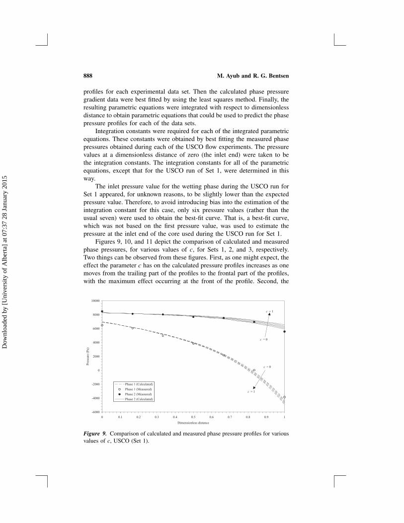
profiles for each experimental data set. Then the calculated phase pressuregradient data were best fitted by using the least squares method. Finally, theresulting parametric equations were integrated with respect to dimensionlessdistance to obtain parametric equations that could be used to predict the phasepressure profiles for each of the data sets.

Integration constants were required for each of the integrated parametricequations. These constants were obtained by best fitting the measured phasepressures obtained during each of the USCO flow experiments. The pressurevalues at a dimensionless distance of zero (the inlet end) were taken to bethe integration constants. The integration constants for all of the parametricequations, except that for the USCO run of Set 1, were determined in thisway.

The inlet pressure value for the wetting phase during the USCO run forSet 1 appeared, for unknown reasons, to be slightly lower than the expectedpressure value. Therefore, to avoid introducing bias into the estimation of theintegration constant for this case, only six pressure values (rather than theusual seven) were used to obtain the best-fit curve. That is, a best-fit curve,which was not based on the first pressure value, was used to estimate thepressure at the inlet end of the core used during the USCO run for Set 1.

Figures 9, 10, and 11 depict the comparison of calculated and measuredphase pressures, for various values of c, for Sets 1, 2, and 3, respectively.Two things can be observed from these figures. First, as one might expect, theeffect the parameter c has on the calculated pressure profiles increases as onemoves from the trailing part of the profiles to the frontal part of the profiles,with the maximum effect occurring at the front of the profile. Second, the

Figure 9. Comparison of calculated and measured phase pressure profiles for variousvalues of c, USCO (Set 1).

Dow

nloa

ded

by [

Uni

vers

ity o

f A

lber

ta]

at 0

7:37

28

Janu

ary

2015

Experimental Testing of Interfacial Coupling 889

Figure 10. Comparison of calculated and measured phase pressure profiles forvarious values of c, USCO (Set 2).

magnitude of the effect is small, being approximately of the same order asthe error in the data. Consequently, because the data were not measured withsufficient precision, it is not possible to estimate the magnitude of c, nor is itpossible to comment definitively on the adequacy of the theory on capillarycoupling.

Figure 11. Comparison of calculated and measured phase pressure profiles forvarious values of c, USCO (Set 3).

Dow

nloa

ded

by [

Uni

vers

ity o

f A

lber

ta]

at 0

7:37

28

Janu

ary

2015

890 M. Ayub and R. G. Bentsen

In an attempt to determine the best estimate for c, the error sum ofsquares (SSE) was determined for each calculated and measured (best-fitted)phase pressure profile for all of the runs. The error sum of squares wascalculated by using:

SSE =n∑

j=1

(yj − yj )2 (57)

where the yj are the measured best-fitted pressure values, the yj are thecalculated phase pressure values, and n is the total number of phase pressurevalues along the core. Figures 12, 13, and 14 depict plots of SSE versus c forexperimental Sets 1, 2, and 3, respectively. Because of the lack of sufficientprecision in the experimental data, it is difficult to analyze these plots.

For the wetting phase, the minimum value of the error sum of squares,SSE , occurs, for all three experimental sets, when c equals 1. When c

equals 1, both the wetting and nonwetting phase pressure gradients [seeEqs. (7) and (55)] contribute to the flow of the wetting phase, and the en-tire fluid-fluid interface of the first RMS is composed of Phase 1-Phase 2interface. For the nonwetting phase, the minimum value of SSE , for all threedata sets, occurs when c equals 0. When c equals 0, only the nonwettingphase pressure gradient contributes to the flow of the nonwetting phase [seeEqs. (80) and (56)], and the entire fluid-fluid interface of the second RMSis composed of fluid 2-fluid 2 interface. Neither the scenario for the wettingphase nor that for the nonwetting phase is physically plausible. Presumably,this lack of plausibility arises because of the lack of sufficient precision inthe experimental data.

Figure 12. Error sum of squares versus c (Set 1).

Dow

nloa

ded

by [

Uni

vers

ity o

f A

lber

ta]

at 0

7:37

28

Janu

ary

2015

Experimental Testing of Interfacial Coupling 891

Figure 13. Error sum of squares versus c (Set 2).

Inasmuch as c is a fraction, it must vary between 0 and 1. As can beseen from Figures 9, 10, and 11, varying c from 0 to 1 had very little impacton the predicted pressures. To be specific, increasing c from 0 to 1 caused anincrease, at the front of a nonwetting profile (dimensionless distance equal toone), in the nonwetting pressure of about 1 kPa. Such a change in pressure isclose to the limit of what can be measured accurately, using the experimental

Figure 14. Error sum of squares versus c (Set 3).

Dow

nloa

ded

by [

Uni

vers

ity o

f A

lber

ta]

at 0

7:37

28

Janu

ary

2015

892 M. Ayub and R. G. Bentsen

apparatus used in this study. Because c has such a small impact on thepredicted values of pressure, it is suggested that the theoretical value of c,0.5, be used. Support for this suggestion, can be found in Steady-Stae Methodand in the study by Bentsen (1998).

DISCUSSION

Capillary Coupling Parameter

As noted in Construction of Equations for Capillary Coupling Parameters, inisotropic, homogeneous, natural porous media, α cannot take on the limitingvalues of 0 and 1, because, for such values, the porous medium ceases toexist. Such need not always be the case. Suppose the porous medium isbeing modeled as a bundle of capillary tubes (channels). If the channels arebounded entirely by fluid-solid surface, α = 1 (φ = 0); that is, there canbe no capillary coupling between adjacent channels that are flowing wettingand nonwetting fluids, respectively. Moreover, because there is no capillarycoupling, the magnitude of the driving force causing imbibition (Bentsen,2001), (1 − φ)∂Pc/∂x, takes on its maximal value. On the other hand, ifthe channels are assumed to be bounded completely by fluid-fluid interface,the displacement would be taking place in free space, rather than withinthe confines of a porous medium. Such an assumption permits the maximumamount of interfacial coupling to take place; that is, α = 0 (φ = 1). However,because there is no porous medium, no imbibition can take place. Thus,the magnitude of the imbibition driving force, (1 − φ)∂Pc/∂x, takes on itsminimal value, zero (Bentsen, 2001).

When a wetting fluid imbibes into a porous medium, high-energy (non-wetting) surface is replaced by lower-energy (wetting) surface, resulting in adecrease in the amount of surface free energy stored in the fluid-solid surfacesin the porous medium. Moreover, the surface free energy that is released, as aconsequence of the decrease in stored surface free energy, provides a sourceof energy to drive the imbibition process. In a homogeneous, isotropic porousmedium, the amount of solid surface area, in any given plane, is proportionalto 1 − φ. If it is supposed that the amount of solid surface over which thethree-phase line of contact moves is proportional to 1 − φ, then the netamount of surface free energy released to drive the imbibition process mustalso be proportional to 1 − φ. If such is the case, the imbibition (capillarypressure) driving force per unit volume will, as well, be proportional to 1 − φ.Such a point of view is consistent with the idea that the imbibition drivingforce per unit volume, ∂Pc/∂x, should be reduced by the factor 1 − φ.

Experimental Testing

The prime objective of this study was to gain a better understanding of theinterfacial coupling phenomena that may occur during two-phase flow through

Dow

nloa

ded

by [

Uni

vers

ity o

f A

lber

ta]

at 0

7:37

28

Janu

ary

2015

Experimental Testing of Interfacial Coupling 893

porous media. Whether cross effects between two fluids flowing througha porous medium exist has been a matter for debate for the last coupleof decades. Several views about the quantitative significance of interfacialcoupling and about its physical origin are available in the literature (Ayuband Bentsen, 1999). Based on the literature review presented in Ayub andBentsen (1999), three main schools of thought can be identified. First, thereare those who believe that interfacial coupling effects are significant; second,there are those who argue that interfacial coupling effects are small, and that,consequently, they can be neglected; and third, there are those who believethat interfacial coupling effects do not exist.

Most of the researchers who belong to the first school of thought believethat interfacial coupling is due to momentum being transferred across thefluid-fluid interfaces that exist in a porous medium. However, Zarcone andLenormand (1994), on the basis of experimental evidence, and Rakotoma-lala et al. (1995), on the basis of theoretical analysis, demonstrated that thecontribution of viscous coupling to the flow of a given phase is negligible(of order 10−2). If viscous coupling is negligibly small, an additional type ofcoupling must be postulated, if one is to explain the experimental observation(Lelièvre, 1966; Bourbiaux and Kalaydjian, 1990; Bentsen and Manai, 1993)that the magnitude of countercurrent mobilities is significantly smaller, fora given phase and saturation, than that of cocurrent mobilities. Babchin andYuan (1997) and Bentsen (2001) suggest that the needed additional interfacialcoupling may arise because of the capillarity of the porous medium.

The fact that the mobilities determined in a countercurrent experiment areless than those determined in a cocurrent experiment cannot be explained, ifone assumes that the conventional transport equations describe correctly two-phase flow through porous media. This is because the conventional equationsare incapable of accounting for interfacial coupling between the two flowingphases. Consequently, if interfacial coupling is to be accounted for prop-erly, use must be made of the newly formulated transport equations. In thisstudy, a partitioning concept was introduced into Kalaydjian’s (1987) trans-port equations to construct modified equations to study interfacial couplingin two-phase flow. Moreover, an attempt was made to test experimentally themodified transport equations.

Two methods, a steady-state method and an unsteady-state method, wereused to test experimentally the modified transport equations. Each of thesemethods requires data from two separate experiments. Implicit in the useof two experiments to test the theory is the assumption that the porousmedia-fluid systems used in the two experiments are identical. Because mi-nor changes in wetting, saturation history, packing, and so forth can have asignificant impact on, for example, the shape of relative permeability curves,it was not possible to satisfy this requirement in this study. This made theinterpretation of the data more difficult.

The steady-state method requires data from SSCO and SSCT flow exper-iments. Using this method and data collected by Manai (1991), it was foundthat there was good agreement between the magnitude of the experimentally

Dow

nloa

ded

by [

Uni

vers

ity o

f A

lber

ta]

at 0

7:37

28

Janu

ary

2015

894 M. Ayub and R. G. Bentsen

determined capillary coupling parameters and those predicted theoretically.However, because of the inability to obtain identical porous media-fluid sys-tems in the two experiments, it was not possible to use the steady-state methodto ascertain the magnitude of the viscous coupling parameters.

To implement the unsteady-state method, data from SSCO and USCO ex-periments are needed. Using data collected by Ayub (2000), an attempt wasmade to determine experimentally the magnitude of the capillary coupling pa-rameters. Unfortunately, for the most part, this attempt was unsuccessful. Thiswas because, as can be seen in Figures 9, 10, and 11, the magnitude of the in-terfacial coupling effects, when using SSCO and USCO flow experiments, wasof the same order as the error in the experimental data. This makes it difficult,when using the unsteady-state method, to argue convincingly that the modi-fied transport equations are valid, or that a correction for interfacial couplingis even needed. Because the unsteady-state method is based on the assump-tion that viscous coupling effects are negligibly small, it was not possible touse this method to estimate the magnitude of the viscous coupling parameters.

CONCLUDING REMARKS

In this study, defining equations for the capillary coupling parameters, αci ,i = 1, 2, and the viscous coupling parameters, αvi , i = 1, 2, have beenconstructed. Moreover, these equations, together with a modified form ofKalaydjian’s transport equations, have been used to analyze interfacial cou-pling in two-phase flow through porous media. On the basis of the analysiscarried out, it is argued that capillary coupling has no effect on steady-state,cocurrent flow, and only a small effect on unsteady-state, cocurrent flow.Moreover, it is suggested that capillary coupling has a significant impact onsteady-state, countercurrent flow.

Two methods were used to test experimentally the modified transportequations. The data from two sets of steady-state, cocurrent, and counter-current flow experiments, together with the first (steady-state) method, wereused to test experimentally the modified transport equations. Good agreementwas found between the magnitude of the experimentally determined capillarycoupling parameters and those predicted theoretically. Because the porousmedia-flow systems were not identical in the two experiments, it was notpossible to estimate the magnitude of the viscous coupling parameters.

The data from three sets of cocurrent, steady-state, and unsteady-stateflow experiments were used also to test experimentally the modified transportequations. In these experiments, nonwetting fluids having two different vis-cosities, and porous media having two different grain size distributions wereused. In the first approach used to test the theory, no definitive conclusionscould be drawn, because of a lack of sufficient precision in the measured data,with respect to either the magnitude of the capillary coupling parameters, orthe adequacy of the capillary coupling theory. In the second approach used to

Dow

nloa

ded

by [

Uni

vers

ity o

f A

lber

ta]

at 0

7:37

28

Janu

ary

2015

Experimental Testing of Interfacial Coupling 895

test the theory, it appeared that the predicted pressure profiles were consistentwith those that had been measured. However, again because of a lack of suf-ficient precision in the measured data, it was not possible to obtain a reliableestimate of the capillary coupling parameters, or to comment definitively onthe adequacy of the theory. Because of the lack of precision in the measureddata, it was not possible to comment on whether viscosity ratio, or grain-sizedistribution, has any impact on the capillary coupling parameters.

Of the two methods used to test the theory, the steady-state methodwas clearly the more successful. Consequently, it is recommended that, infuture studies on interfacial coupling, one of the two experiments used to testthe theory should be a countercurrent flow experiment, because interfacialcoupling effects are larger in such flow.

NOMENCLATURE

a Dimensionless parameter appeared in equationR12 = 1 − a[1 − S]

Ab Bulk area of the RMScij Fraction of fluid-fluid interface that is Phase i-Phase j interface;

i, j = 1, 2C Parameter that controls the amount of viscous couplingFij Force acting on the Phase i-Phase j portion of the fluid-fluid

portion of the RMS; i, j = 1, 2Fis Force acting on the phase i-solid part of the RMS; i = 1, 2kij Generalized effective permeability for phase i; i, j = 1, 2kri Steady-state cocurrent relative permeability for phase i; i = 1, 2k∗ri Steady-state countercurrent relative permeability for phase i;

i = 1, 2(kri)n Normalized steady-state cocurrent relative permeability for

phase i; i = 1, 2(k∗

ri)n Normalized steady-state countercurrent relative permeability forphase i; i = 1, 2

M Endpoint mobility ration Number of pressure values along the core holderpi Pressure of phase i; i = 1, 2pi Average pressure of phase i acting at the midpoint of an RMS;

i = 1, 2Pc Capillary pressureR12 Function relating the pressure gradient in Phase 1 to that in

Phase 2RES Representative elementary surfaceRHS Right-hand side of an equationRMS Representative macroscopic surfaceS Normalized wetting phase saturation

Dow

nloa

ded

by [

Uni

vers

ity o

f A

lber

ta]

at 0

7:37

28

Janu

ary

2015

896 M. Ayub and R. G. Bentsen

S1 Saturation for Phase 1SSE Eerror sum of squaresSSCO Steady-state cocurrentSSCT Steady-state countercurrentUSCO Unsteady-state cocurrentvi Darcy velocity of phase i; i = 1, 2x ength of porous mediumyj Measured (fitted) pressure values along the core-holder; j = 1, nyj Calculated pressure values along the core-holder; j = 1, n1 Subscript for wetting phase2 Subscript for nonwetting phaseαi Interfacial coupling parameter; i = 1, 2αci Capillary coupling parameter; i = 1, 2αvi Viscous coupling parameter; i = 1, 2λij Generalized mobility of phase i; i, j = 1, 2λ◦i Mobility determined by using cocurrent flow for phase i; i = 1, 2

λ∗w Mobility determined by using countercurrent flow for phase i;

i = 1, 2λ◦w Weighted mobility used for dimensional consistency

φ Porosity of a porous mediumµi Viscosity of phase i; i = 1, 2

REFERENCES

Ayub, M., and Bentsen, R. G. (2001). Petroleum Sci. Technol. 19(9&10):1129.Ayub, M., and Bentsen, R. G. (1999). J. Petroleum Sci. Eng. 23:13.Ayub, M., and Bentsen, R. G. (2000). J. Can. Petroleum Technol. 39(9):54.Ayub, M. (2000). The experimental testing of the impact of interfacial cou-

pling on two-phase flow in porous media. Ph.D. thesis. Alberta, Canada:University of Alberta, Canada.

Babchin, A. J., and Yuan, J. (1997). Transport Porous Media 26:225.Bacri, J., Chaouche, M., and Salin, D. (1990). C. R. Acad. Sci. 311(II):591.Bentsen, R. G., and Manai, A. A. (1991). AOSTRA J. Res. 7:169.Bentsen, R. G., and Manai, A. A. (1993). Transport Porous Media 11:243.Bentsen, R. G. (2003). Transport Porous Media 51:103.Bentsen, R. G. (1992). AOSTRA J. Res. 8:159.Bentsen, R. G. (1994). Transport Porous Media 17:133.Bentsen, R. G. (1998). J. Petroleum Sci. Eng. 21:27.Bentsen, R. G. (1998). J. Petroleum Sci. Eng. 19:177.Bentsen, R. G. (2001). Transport Porous Media 44:109.Bourbiaux, B. J., and Kalaydjian, F. J. (1990). SPERE 5:361.Chang, S. (1996). Experimental apparatus for measurement of generalized

permeability coefficients using steady state and unsteady state, cocur-rent and countercurrent flow methods. M.Sc. thesis. Alberta, Canada:University of Alberta.

Dow

nloa

ded

by [

Uni

vers

ity o

f A

lber

ta]

at 0

7:37

28

Janu

ary

2015

Experimental Testing of Interfacial Coupling 897

Chatenever, A., and Calhoun, J. C. Jr. (1952). Trans. AIME 195:149.de Gennes, P. G. (1983). Physicochem. Hydrodynam. 4:175.de la Cruz, V., and Spanos, T. J. T. (1983). AIChE J. 29(5):854.de la Cruz, V., Sahay, P. N., and Spanos, T. J. T. (1993). Proc. R. Soc. London

A443:247.de La Cruz, V., Spanos, T. J. T., and Yang, D. (1995). Lett. Math. Phys.

19:67.Dullien, F. A. L., and Dong, M. (1996). Transport Porous Media 25:97.Goode, P. A. (1991). Momentum transfer across fluid-fluid interfaces in

porous media. Ph.D thesis. Edinburgh, UK: Heriot-Watt University.Kalaydjian, F. (1987). Transport Porous Media 2:537.Katchalsky, A., and Curran, P. F. (1967). Nonequilibrium Thermodynamics

in Biophysics. Cambridge, MA: Harvard University Press.Lelièvre, R. F. (1966). Etude d’ écoulements disphasiques permanents à

contre-courants en milieu poreux—Comparaison avec les écoulementsde même sens (in French). Ph.D. thesis. Toulouse, France: University ofToulouse.

Liang, Q., and Lohrenz, J. (1994). Transport Porous Media 15:71.Liang, Q. (1993). Interaction between immiscible phases flowing at different

velocities in porous media. D.E. thesis. Lubbock, Texas: Louisiana TechUniversity.

Manai, A. A. (1991). The measurement of cocurrent and countercurrent rel-ative permeabilities and their use to estimate generalized relative perme-abilities. M.S. thesis. Alberta, Canada: University of Alberta.

Muskat, M. (1982). The Flow of Homogeneous Fluids through Porous Media.Boston, MA: International Human Resources Development Corporation.

Rakotomalala, N., Salin, D., and Yortsos, C. Y. (1995). App. Sci. Res. 55:155.Rapoport, L. A., and Leas, W. J. (1953). Trans. AIME 198:139.Rose, W. (1990). Transport Porous Media 5:97.Rose, W. (1988). Transport Porous Media 32:163.Whitaker, S. (1986). Transport Porous Media 1:105.Zarcone, C., and Lenormand, R. (1994). C. R. Acad. Sci. 318(II):1429.

Dow

nloa

ded

by [

Uni

vers

ity o

f A

lber

ta]

at 0

7:37

28

Janu

ary

2015