Citation: Yang, Y.; Zhu, W.; Ji, Y.;

Wang, T.; Zhao, G. Interfacial

Properties of H2O+CO2+Oil

Three-Phase Systems: A Density

Gradient Theory Study. Atmosphere

2022, 13, 625. https://doi.org/

10.3390/atmos13040625

Academic Editor: Jaroslaw

Krzywanski

Received: 25 March 2022

Accepted: 12 April 2022

Published: 14 April 2022

Publisher’s Note: MDPI stays neutral

with regard to jurisdictional claims in

published maps and institutional affil-

iations.

Copyright: © 2022 by the authors.

Licensee MDPI, Basel, Switzerland.

This article is an open access article

distributed under the terms and

conditions of the Creative Commons

Attribution (CC BY) license (https://

creativecommons.org/licenses/by/

4.0/).

atmosphere

Article

Interfacial Properties of H2O+CO2+Oil Three-Phase Systems:A Density Gradient Theory StudyYafan Yang 1,2,* , Weiwei Zhu 3, Yukun Ji 1,2, Tao Wang 2,4 and Guangsi Zhao 1,2,*

1 State Key Laboratory for Geomechanics and Deep Underground Engineering,China University of Mining and Technology, Xuzhou 221116, China; yukun.ji@cumt.edu.cn

2 School of Mechanics and Civil Engineering, China University of Mining and Technology,Xuzhou 221116, China; taowang@cumt.edu.cn

3 Department of Engineering Mechanics, Tsinghua University, Beijing 100084, China;weiweizhu@mail.tsinghua.edu.cn

4 State Key Laboratory of Coal Mining and Clean Utilization, China Coal Research Institute,Beijing 100013, China

* Correspondence: yafan.yang@cumt.edu.cn (Y.Y.); zhaoguangsi@cumt.edu.cn (G.Z.)

Abstract: The interfacial property of H2O+CO2+oil three-phase systems is crucial for CO2 floodingand sequestration processes but was not well understood. Density gradient theory coupled withPC-SAFT equation of state was applied to investigate the interfacial tension (IFT) of H2O+CO2+oil(hexane, cyclohexane, and benzene) systems under three-phase conditions (temperature in the rangeof 323–423 K and pressure in the range of 1–10 MPa). The IFTs of the aqueous phase+vapor phasein H2O+CO2+oil three-phase systems were smaller than the IFTs in H2O+CO2 two-phase systems,which could be explained by enrichment of oil in the interfacial region. The difference between IFTsof aqueous phase+vapor phase in the three-phase system and IFTs in H2O+CO2 two-phase systemwas largest in the benzene case and smallest in the cyclohexane case due to different degrees of oilenrichment in the interface. Meanwhile, CO2 enrichment was observed in the interfacial region ofthe aqueous phase+oil-rich phase, which led to the reduction of IFT with increasing pressure whiledifferent pressure effects were observed in the H2O+oil two-phase systems. The effect of CO2 onthe IFTs of aqueous phase+benzene-rich phase interface was small in contrast to that on the IFTsof aqueous phase+alkane (hexane or cyclohexane)-rich phase interface. H2O had little effect on theinterfacial properties of the oil-rich phase+vapor phase due to the low H2O solubilities in the oil andvapor phase. Further, the spreading coefficients of H2O+CO2 in the presence of different oil followedthis sequence: benzene > hexane > cyclohexane.

Keywords: carbon dioxdie flooding; three-phase system; interfacial properties; spreading coefficient;density gradient theory; PC-SAFT

1. Introduction

Recently, many countries around the world have targeted net-zero carbon emissionsin the following few decades to mitigate global warming [1–3]. CO2 flooding techniqueshave demonstrated great potential in offsetting greenhouse emissions and increasing oilrecovery efficiency at the same time [4–6]. Although CO2 miscible flooding is one ofthe most effective methods of enhancing oil recovery, a significant amount of reservoirconditions cannot meet the miscible requirements because of either technical issues oreconomic considerations [7]. Hence CO2 near-miscible or immiscible flooding may beapplied when the pressure condition does not allow CO2 to fully dissolve in oil [8]. Duringnear-miscible or immiscible water alternating gas injection processes, interfacial tension(IFT) of H2O+CO2+oil three-phase systems is of great importance since it can determinethe capillary force that displaces oil and stores CO2 in geological formations [4,9].

Atmosphere 2022, 13, 625. https://doi.org/10.3390/atmos13040625 https://www.mdpi.com/journal/atmosphere

Atmosphere 2022, 13, 625 2 of 18

There has been a considerable number of studies on the interfacial properties of two-phase systems containing H2O, CO2 and/or oil [10–22]. Generally, the IFT of H2O+CO2two-phase system decreases with increasing temperature and pressure [10,16,20]. However,at relatively high pressures, the IFT increases with increasing pressure [17]. The IFT ofH2O+oil two-phase systems usually increases with decreasing temperature and increasingpressure [11,23–25]. When H2O+oil two-phase systems are in contact with CO2 undermiscible conditions, the IFT increases with decreasing CO2 mole fraction mainly becauseof the positive surface excess of CO2 in the interface [19,21,24]. The IFT in the oil+CO2two-phase system decreases with pressure and at elevated temperatures, the reductionof IFT due to pressure increment decreases [18,26,27]. Although a few studies on theinterfacial properties of water+gas+oil three-phase systems have been carried out [28–32],interfacial properties of H2O+CO2+oil three-phase system have not been investigated yet.

In this work, we studied the interfacial properties of H2O+CO2+oil three-phase sys-tems at different temperatures (323, 373, and 423 K) and pressures (1–10 MPa). The tem-perature and pressure conditions chosen here are typical reservoir conditions during CO2near-miscible or immiscible flooding [33,34]. The composition of crude oil is complex, andthe predominant components are aliphatic, alicyclic and aromatic hydrocarbons [35–37].Hence, hexane, cyclohexane, and benzene were selected to represent these hydrocarbontypes in this study. The IFTs were calculated by density gradient theory (DGT) coupledwith the perturbed-chain statistical associating fluid theory (PC-SAFT) equation of state(EoS). The component density distributions and surface excess in the interfacial region wereanalyzed to understand the behavior of IFT of three-phase systems at geological conditions.

2. Theoretical Details

PC-SAFT EoS was applied to estimate the bulk properties of fluid mixtures. The EoScan be expressed via the compressibility factor Z [38,39]:

Z = 1 + Zhc + Zdisp + Zassoc, (1)

where Zhc is the hard-chain term, Zdisp is the dispersive part, and Zassoc represents thecontribution due to association. Z is a function of the segment number mi, the segmentdiameter σi, and the segment energy parameter εi. H2O was modeled with 4C associationscheme, and CO2 and benzene can cross-associate with H2O [40]. The parameters for a pairof unlike segments were estimated using the Lorentz-Berthelot combining rules [38]:

σij =12(σi + σj), (2)

εij =√

εiεj(1 − kij) (3)

where kij is the binary interaction parameter. The EoS parameters are given in Tables 1 and 2.Most of the parameters were taken from previous studies [21,22,24,38,41,42]. The missingparameter was fitted based on experimental data [43].

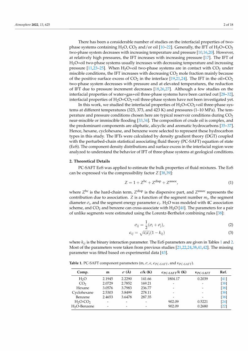
Table 1. PC-SAFT component parameters (m, σ, ε, εPC-SAFT , and κPC-SAFT).

Comp. m σ (Å) ε/k (K) εPC-SAFT /k (K) κPC-SAFT Ref.

H2O 2.1945 2.2290 141.66 1804.17 0.2039 [41]CO2 2.0729 2.7852 169.21 - - [38]

Hexane 3.0576 3.7983 236.77 - - [38]Cyclohexane 2.5303 3.8499 278.11 - - [38]

Benzene 2.4653 3.6478 287.35 - - [38]H2O-CO2 - - - 902.09 0.5221 [24]

H2O-Benzene - - - 902.09 0.2680 [22]

Atmosphere 2022, 13, 625 3 of 18

Table 2. PC-SAFT binary interaction parameter (kij) (T is temperature in K). ‘Expt.’ indicates theexperiment reference for fitting the parameter.

Pair kij Ref.

H2O-CO2 3.8257 × 10−4·T − 2.8007 × 10−2 [24]H2O-hexane −3.0873 × 10−6·T2 + 2.5828 × 10−3·T − 3.3410 × 10−1 [21]

H2O-Cyclohexane −2.6448 × 10−6·T2 + 2.1778 × 10−3·T − 2.3225 × 10−1 [21]H2O-Benzene 8.7902 × 10−5·T + 1.2922×10−1 [22]CO2-Hexane 0.0711 [42]

CO2-Cyclohexane 0.1300 [38]CO2-Benzene 0.0881 Expt. [43]

PC-SAFT EoS was coupled with the DGT for the estimation of interfacial properties.Briefly, for a planar interface of area A, the Helmholtz free energy is given as [44,45]:

F = A∫ +∞

−∞

[f0(n) +

12 ∑

i∑

jcij

dni

dzdnj

dz

]dz, (4)

where f0 denotes the Helmholtz free energy density of the homogeneous fluid at the localdensity n, dni/dz represents the local density gradient of the ith component. The crossinfluence parameter cij is defined as [46–48]:

cij = (1 − βij)√

ciicjj, (5)

where cii and cjj represent the pure component influence parameters, and βij denote thebinary interaction coefficient. These parameters were given in Tables 3 and 4, and theywere fitted in previous studies of two-phase systems [21,22,42,49].

Table 3. DGT (PC-SAFT) influence parameter (cii).

Comp. cii (10−20 J m5 mol−2) Ref.

H2O 1.4412 [49]CO2 2.4280 [24]

Hexane 32.8347 [21]Cyclohexane 34.1111 [21]

Benzene 23.2970 [22]

Table 4. DGT (PC-SAFT) binary interaction coefficient (βij) for pairs.

Pair βij Ref.

H2O-CO2 0.39 [24]H2O-hexane 0.54 [21]

H2O-Cyclohexane 0.55 [21]H2O-Benzene 0.24 [22]CO2-Hexane 0.04 -

CO2-Cyclohexane 0.04 -CO2-Benzene 0.07 -

In equilibrium, the density profiles across the interface were evaluated through the min-imization of the free energy by solving the corresponding Euler-Lagrange equation [44,45]:

∑j

cijd2nj

dz2 = µ0i (n1(z), . . . , nNc(z))− µi for i, j = 1, . . . , Nc, (6)

where µ0i is the chemical potential of the ith component in the bulk phase (µ0

i ≡ ( ∂ f0∂ni

)T,V,nj ),µi represents the chemical potential of the ith component and Nc denotes the total number

Atmosphere 2022, 13, 625 4 of 18

of components. These equations were solved together with the boundary conditionsobtained from three-phase flash calculations [50]:

ni = nIi at z = 0

ni = nI Ii at z = l,

(7)

where nIi and nI I

i represent the bulk densities of the coexisting phases and l denotes theinterfacial thickness of one interface in three-phase system. When the equilibrium densityprofiles were available, the interfacial tension (γ) was estimated as follows [44,45]:

γ =∫ +∞

−∞∑

i∑

jcij

dni

dzdnj

dzdz (8)

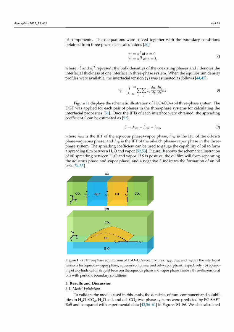
Figure 1a displays the schematic illustration of H2O+CO2+oil three-phase system. TheDGT was applied for each pair of phases in the three-phase systems for calculating theinterfacial properties [51]. Once the IFTs of each interface were obtained, the spreadingcoefficient S can be estimated as [52]:

S = λwv − λow − λov, (9)

where λwv is the IFT of the aqueous phase+vapor phase, λow is the IFT of the oil-richphase+aqueous phase, and λov is the IFT of the oil-rich phase+vapor phase in the three-phase system. The spreading coefficient can be used to gauge the capability of oil to forma spreading film between H2O and vapor [52,53]. Figure 1b shows the schematic illustrationof oil spreading between H2O and vapor. If S is positive, the oil film will form separatingthe aqueous phase and vapor phase, and a negative S indicates the formation of an oillens [54,55].

Figure 1. (a) Three-phase equilibrium of H2O+CO2+oil mixtures. γwv, γwo, and γov are the interfacialtensions for aqueous+vapor phase, aqueous+oil phase, and oil+vapor phase, respectively. (b) Spread-ing of a cylindrical oil droplet between the aqueous phase and vapor phase inside a three-dimensionalbox with periodic boundary conditions.

3. Results and Discussion3.1. Model Validation

To validate the models used in this study, the densities of pure component and solubil-ities in H2O+CO2, H2O+oil, and oil+CO2 two-phase systems were predicted by PC-SAFTEoS and compared with experimental data [43,56–61] in Figures S1–S6. We also calculated

Atmosphere 2022, 13, 625 5 of 18

the IFT of H2O+CO2, H2O+oil, and oil+CO2 two-phase systems and compared the IFTswith experimental data [10–15] as shown in Figures S7–S9. Good agreement was obtainedbetween theory and experiment. For example, the maximum IFT deviation is around4 mN/m. Figures S10–S19 show the calculated density distributions and component sur-face excess [16,18,62] in the two-phase systems. Although it is challenging to measure thecomponent distributions in the interfacial region in experiment [63], the calculated inter-facial properties were in reasonable agreement with previous simulation and theoreticalstudies of two-phase systems [16,18,20–22].

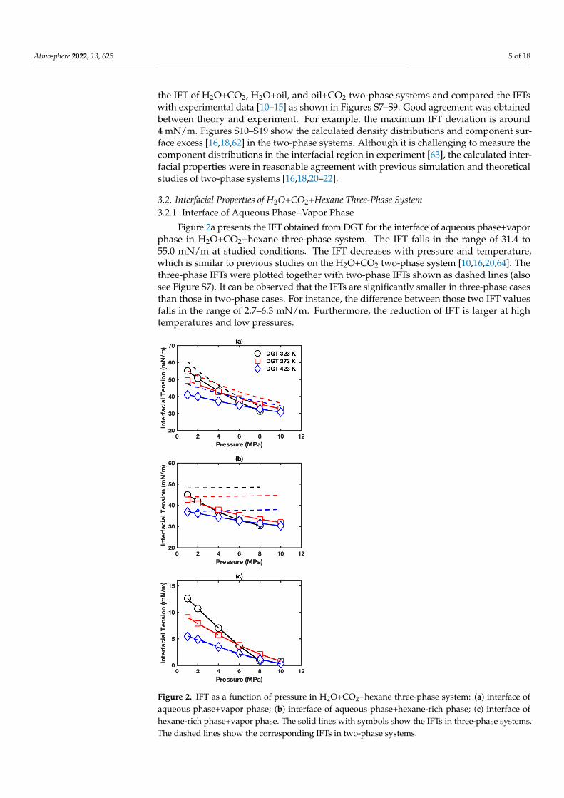
3.2. Interfacial Properties of H2O+CO2+Hexane Three-Phase System3.2.1. Interface of Aqueous Phase+Vapor Phase

Figure 2a presents the IFT obtained from DGT for the interface of aqueous phase+vaporphase in H2O+CO2+hexane three-phase system. The IFT falls in the range of 31.4 to55.0 mN/m at studied conditions. The IFT decreases with pressure and temperature,which is similar to previous studies on the H2O+CO2 two-phase system [10,16,20,64]. Thethree-phase IFTs were plotted together with two-phase IFTs shown as dashed lines (alsosee Figure S7). It can be observed that the IFTs are significantly smaller in three-phase casesthan those in two-phase cases. For instance, the difference between those two IFT valuesfalls in the range of 2.7–6.3 mN/m. Furthermore, the reduction of IFT is larger at hightemperatures and low pressures.

Figure 2. IFT as a function of pressure in H2O+CO2+hexane three-phase system: (a) interface ofaqueous phase+vapor phase; (b) interface of aqueous phase+hexane-rich phase; (c) interface ofhexane-rich phase+vapor phase. The solid lines with symbols show the IFTs in three-phase systems.The dashed lines show the corresponding IFTs in two-phase systems.

Atmosphere 2022, 13, 625 6 of 18

Figure 3a,d display density distributions of H2O, CO2, and hexane as calculated byDGT in the interfacial region between the aqueous phase and vapor phase in the three-phase system at 6 MPa and different temperatures. Corresponding cases at 1 MPa are givenin Figure S20a,d. The shapes of H2O and CO2 density profiles are similar to those of theH2O+CO2 two-phase system [16,20,64] (also see Figure S10). The density profile of H2O isclose to a hyperbolic tangent function. Enrichment of CO2 in the interfacial region can beobserved in all cases. Remarkably, enrichment of hexane in the interfacial region is alsoseen. The enrichment of hexane is likely due to the hydrophobic interaction between H2Oand oil.

Figure 3. Equilibrium distributions of different species in H2O+CO2+hexane three-phase system at323 K, 6 MPa (left panels) and 423 K, 6 MPa (right panels): (a,d) interface of aqueous phase+vaporphase (top panels); (b,e) interface of aqueous phase+hexane-rich phase (middle panels); (c,f) interfaceof hexane-rich phase+vapor phase (bottom panels). Solid, dashed, and dotted lines represent H2O,hexane, and CO2, respectively.

Surface excess can gauge the component enrichment in the interfacial region [16,18,62].The behavior of IFT is associated with surface excess through the Gibbs adsorption equa-tion [24,62]. Figure S21a,d show the surface excess of CO2 and hexane (H2O is selected asthe reference). The surface excess of CO2 is consistent with that of the H2O+CO2 two-phasesystem in the previous study [62] (also see Figure S17). The CO2 surface excess decreaseswith increasing temperature, and it increases with increasing pressure. The hexane surface

Atmosphere 2022, 13, 625 7 of 18

excesses are all positive, which gives rise to the reduction of IFT when hexane is includedin the system based on the Gibbs adsorption equation. Hexane surface excess is enhancedby high pressure, possibly because of the relatively higher oil solubility in the vapor phaseat high pressure [27]. High temperature increases the hexane surface excess due to theincrease of oil solubility in vapor at high temperatures.

3.2.2. Interface of Aqueous Phase+Hexane-Rich Phase

Figure 2b presents the IFTs for the interface of aqueous phase+hexane-rich phasein H2O+CO2+hexane three-phase system. The IFT decreases with increasing pressureand temperature, and falls in the range of 30.4 to 44.9 mN/m. As temperature increases,the reduction of IFT due to pressure increment decreases. For example, at 373 K, theIFT decreases by about 10.7 mN/m from 42.6 to 31.9 mN/m when increasing pressurefrom 1 to 10 MPa. While at 423 K, the IFT decreases by around 6.5 nN/m from 36.9 to30.4 mN/m with the same pressure increase. The three-phase IFT data were plottedtogether with H2O+hexane two-phase IFT data as dashed lines (also see Figure S8a). TheIFT in H2O+hexane two-phase system without CO2 behaves significantly different fromthose in the three-phase system. The IFT of H2O+hexane two-phase system increases withincreasing pressure and is larger than that in the three-phase system, especially at lowtemperature and high pressure conditions. For example, at 323 K and 8 MPa, the IFTdifference can be up to 18.1 mN/m.

Figure 3b,e display density profiles of H2O, CO2, and hexane for the interface ofaqueous phase+oil-rich phase in the three-phase system at 6 MPa and different tempera-tures. Corresponding cases at 1 MPa are given in Figure S20b,e. The shape of H2O andhexane density profiles is similar to that of the H2O+hexane two-phase system [21] (also seeFigure S14). The density profiles of H2O and hexane can be approximated by a hyperbolictangent function. Importantly, enrichment of CO2 in the interface is observed in all cases.

Figure S21b,e show the calculated surface excess of CO2 and hexane with H2O asthe reference component. The surface excess of hexane is mostly negative and generallyincreases with temperature. However, in H2O-hexane two-phase system, an oppositetemperature effect was reported [21] (also see Figure S18a). Meanwhile, the CO2 surfaceexcess is positive and increases with pressure and decreases with temperature. Based onthe Gibbs adsorption equation, the effect of pressure on IFT in the three-phase system couldbe mainly explained by the positive CO2 surface excess.

3.2.3. Interface of Hexane-Rich Phase+Vapor Phase

Figure 2c gives the IFTs for the interface of hexane-rich phase+vapor phase in H2O+CO2+hexane three-phase system. The IFTs are almost the same as those in the hexane+CO2two-phase system (also see Figure S9a). The negligible effect of H2O on IFT is likely dueto minor H2O solubility in the oil-rich [24] and vapor [20] phase. Figures 3c,f and S20c,fpresent the density profiles. Only a slight difference can be observed when comparingthem with density profiles in the hexane+CO2 two-phase system shown in Figure S14. Thedifference between CO2 surface excess with hexane as the reference component in the three-phase system (see Figure S21c) and that in the two-phase system (see Figure S19a) is small.Remarkably, positive H2O surface excesses are predicted. As shown in Figure S21f, H2Osurface excesses increase with temperature and generally increase as pressure increases.The positive H2O surface excesses indicate H2O enrichment in the interfacial region.

3.3. Interfacial Properties of H2O+CO2+Cyclohexane Three-Phase System3.3.1. Interface of Aqueous Phase+Vapor Phase

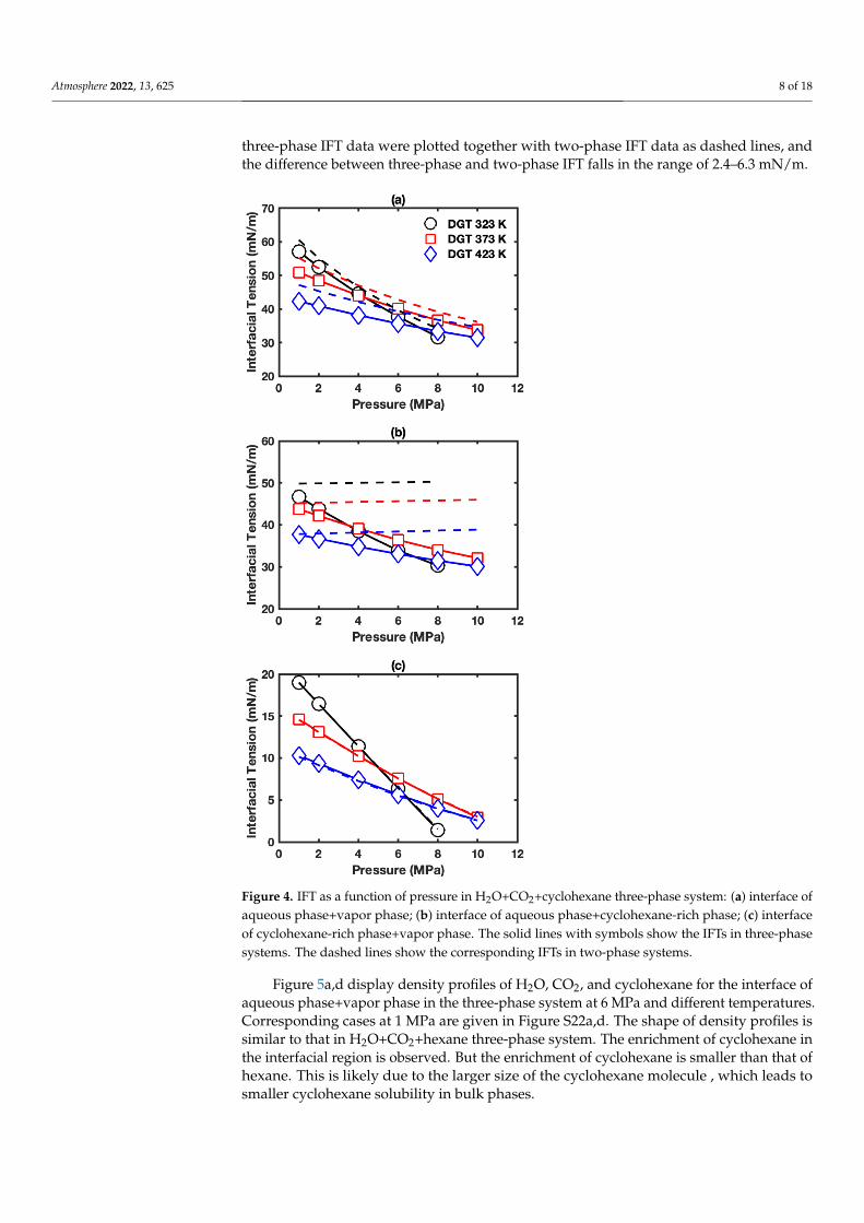
Figure 4a presents the IFTs for the interface of aqueous phase+vapor phase in H2O+CO2+cyclohexane three-phase system. The IFTs decrease with pressure and temperature, similarto the H2O+CO2+hexane three-phase system mentioned above. The IFTs fall in the rangeof 31.7 to 57.1 mN/m, which are slighter higher than the IFTs in H2O+CO2+hexane three-phase system indicating the smaller effect of cyclohexane on IFT than that of hexane. The

Atmosphere 2022, 13, 625 8 of 18

three-phase IFT data were plotted together with two-phase IFT data as dashed lines, andthe difference between three-phase and two-phase IFT falls in the range of 2.4–6.3 mN/m.

Figure 4. IFT as a function of pressure in H2O+CO2+cyclohexane three-phase system: (a) interface ofaqueous phase+vapor phase; (b) interface of aqueous phase+cyclohexane-rich phase; (c) interfaceof cyclohexane-rich phase+vapor phase. The solid lines with symbols show the IFTs in three-phasesystems. The dashed lines show the corresponding IFTs in two-phase systems.

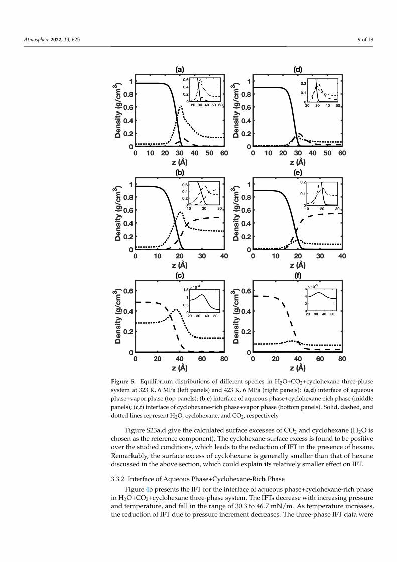
Figure 5a,d display density profiles of H2O, CO2, and cyclohexane for the interface ofaqueous phase+vapor phase in the three-phase system at 6 MPa and different temperatures.Corresponding cases at 1 MPa are given in Figure S22a,d. The shape of density profiles issimilar to that in H2O+CO2+hexane three-phase system. The enrichment of cyclohexane inthe interfacial region is observed. But the enrichment of cyclohexane is smaller than that ofhexane. This is likely due to the larger size of the cyclohexane molecule , which leads tosmaller cyclohexane solubility in bulk phases.

Atmosphere 2022, 13, 625 9 of 18

Figure 5. Equilibrium distributions of different species in H2O+CO2+cyclohexane three-phasesystem at 323 K, 6 MPa (left panels) and 423 K, 6 MPa (right panels): (a,d) interface of aqueousphase+vapor phase (top panels); (b,e) interface of aqueous phase+cyclohexane-rich phase (middlepanels); (c,f) interface of cyclohexane-rich phase+vapor phase (bottom panels). Solid, dashed, anddotted lines represent H2O, cyclohexane, and CO2, respectively.

Figure S23a,d give the calculated surface excesses of CO2 and cyclohexane (H2O ischosen as the reference component). The cyclohexane surface excess is found to be positiveover the studied conditions, which leads to the reduction of IFT in the presence of hexane.Remarkably, the surface excess of cyclohexane is generally smaller than that of hexanediscussed in the above section, which could explain its relatively smaller effect on IFT.

3.3.2. Interface of Aqueous Phase+Cyclohexane-Rich Phase

Figure 4b presents the IFT for the interface of aqueous phase+cyclohexane-rich phasein H2O+CO2+cyclohexane three-phase system. The IFTs decrease with increasing pressureand temperature, and fall in the range of 30.3 to 46.7 mN/m. As temperature increases,the reduction of IFT due to pressure increment decreases. The three-phase IFT data were

Atmosphere 2022, 13, 625 10 of 18

plotted together with H2O+cyclohexane two-phase IFT data as dashed lines (also seeFigure S8b). Similar to the hexane case, the IFTs without CO2 are significantly differentfrom those in the three-phase system. The IFTs of H2O+cyclohexane two-phase systemincrease with increasing pressure and are larger than those in the three-phase system,especially at low temperature and high pressure conditions.

Figure 5b,e display density profiles of H2O, CO2, and cyclohexane for the interface ofaqueous phase+cyclohexane-rich phase in the three-phase system at 6 MPa and differenttemperatures. Corresponding cases at 1 MPa are given in Figure S22b,e. The shape ofH2O and cyclohexane density profiles is similar to that of the H2O+cyclohexane two-phasesystem [21] (also see Figure S12). The density profiles of H2O and cyclohexane can also beapproximated by a hyperbolic tangent function. Enrichment of CO2 is seen in all cases.

Figure S23b,e show the calculated surface excess of CO2 and cyclohexane with H2O asthe reference component. The surface excess of cyclohexane is negative and increases withtemperature. However, in H2O-cyclohexane two-phase system, an opposite temperatureeffect was reported [21] (also see Figure S18b). Meanwhile, the CO2 surface excess ispositive and generally increases with pressure and decreases with temperature. Based onthe Gibbs adsorption equation, the effect of pressure on IFT in the three-phase system canbe mainly explained by the positive CO2 surface excess.

3.3.3. Interface of Cyclohexane-Rich Phase+Vapor Phase

Figure 4c displays the IFTs for the interface of cyclohexane-rich phase+vapor phase inH2O+CO2+cyclohexane three-phase system. Similar to the corresponding case with hexane,the IFTs are almost the same as those in the cyclohexane+CO2 two-phase system (also seeFigure S9b). Figures 5c,f and S22c,f present the corresponding density profiles. Only verylittle difference can be seen comparing them with density profiles in the cyclohexane+CO2two-phase system shown in Figure S15. As expected, the difference between CO2 surface ex-cess in the three-phase system (Figure S23c) and that in the two-phase system (Figure S19b)is minor. As shown in Figure S23f, H2O surface excess is positive, and the H2O surfaceexcess increases with temperature and pressure.

3.4. Interfacial Properties of H2O+CO2+Benzene Three-Phase System3.4.1. Interface of Aqueous Phase+Vapor Phase

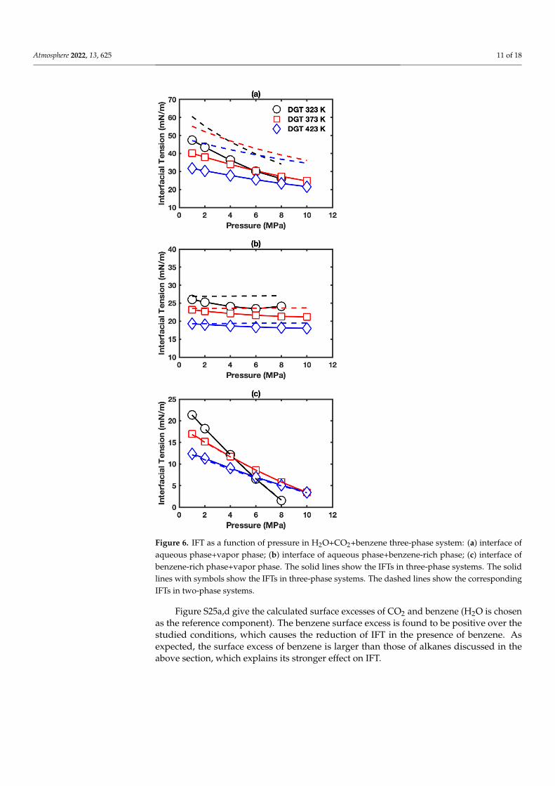
Figure 6a presents the IFTs for the interface of aqueous phase+vapor phase inH2O+CO2+benzene three-phase system. The IFTs decrease with pressure and temperature,similar to the H2O+CO2+alkane (hexane or cyclohexane) three-phase systems mentionedabove. The IFTs fall in the range of 21.6 to 47.4 mN/m, which are much lower than the IFTsin H2O+CO2+alkane three-phase systems. This indicates the strong effect of benzene onIFT than that of alkane possibly due to the strong association between benzene and H2O.The three-phase IFT data were plotted together with two-phase IFT data in dashed lines.The difference between three-phase and two-phase IFT decreases as pressure increases andtemperature decreases, and falls in the range of 8.1–15.5 mN/m.

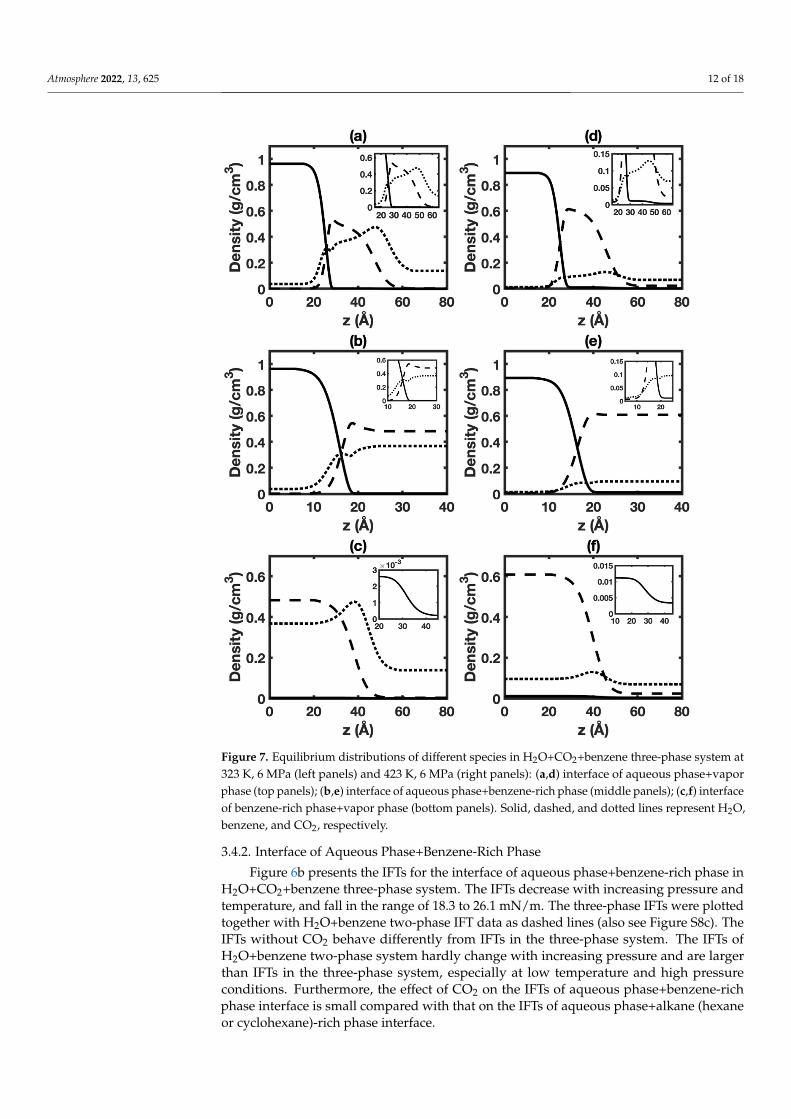
Figure 7a,d displays the density profiles of H2O, CO2, and benzene for the interface ofaqueous phase+vapor phase in the three-phase system at 6 MPa and different temperatures.Corresponding cases at 1 MPa are given in Figure S24a,d. The shape of density profilesis similar to that in H2O+CO2+alkane three-phase system. The enrichment of benzenein the interfacial region is observed. The enrichment of benzene is much stronger thanthose of alkanes, which can be explained by the strong hydrogen bond between H2O andbenzene [65].

Atmosphere 2022, 13, 625 11 of 18

Figure 6. IFT as a function of pressure in H2O+CO2+benzene three-phase system: (a) interface ofaqueous phase+vapor phase; (b) interface of aqueous phase+benzene-rich phase; (c) interface ofbenzene-rich phase+vapor phase. The solid lines show the IFTs in three-phase systems. The solidlines with symbols show the IFTs in three-phase systems. The dashed lines show the correspondingIFTs in two-phase systems.

Figure S25a,d give the calculated surface excesses of CO2 and benzene (H2O is chosenas the reference component). The benzene surface excess is found to be positive over thestudied conditions, which causes the reduction of IFT in the presence of benzene. Asexpected, the surface excess of benzene is larger than those of alkanes discussed in theabove section, which explains its stronger effect on IFT.

Atmosphere 2022, 13, 625 12 of 18

Figure 7. Equilibrium distributions of different species in H2O+CO2+benzene three-phase system at323 K, 6 MPa (left panels) and 423 K, 6 MPa (right panels): (a,d) interface of aqueous phase+vaporphase (top panels); (b,e) interface of aqueous phase+benzene-rich phase (middle panels); (c,f) interfaceof benzene-rich phase+vapor phase (bottom panels). Solid, dashed, and dotted lines represent H2O,benzene, and CO2, respectively.

3.4.2. Interface of Aqueous Phase+Benzene-Rich Phase

Figure 6b presents the IFTs for the interface of aqueous phase+benzene-rich phase inH2O+CO2+benzene three-phase system. The IFTs decrease with increasing pressure andtemperature, and fall in the range of 18.3 to 26.1 mN/m. The three-phase IFTs were plottedtogether with H2O+benzene two-phase IFT data as dashed lines (also see Figure S8c). TheIFTs without CO2 behave differently from IFTs in the three-phase system. The IFTs ofH2O+benzene two-phase system hardly change with increasing pressure and are largerthan IFTs in the three-phase system, especially at low temperature and high pressureconditions. Furthermore, the effect of CO2 on the IFTs of aqueous phase+benzene-richphase interface is small compared with that on the IFTs of aqueous phase+alkane (hexaneor cyclohexane)-rich phase interface.

Atmosphere 2022, 13, 625 13 of 18

Figure 7b,e display density profiles of H2O, CO2, and benzene for the interface ofaqueous phase+benzene-rich phase in the three-phase system at 6 MPa and differenttemperatures. Corresponding cases at 1 MPa are given in Figure S24b,e. The shape ofH2O density profile is similar to that of the H2O+benzene two-phase system [22] (alsosee Figure S13). Enrichment of benzene and CO2 are seen in the interfacial region due torelatively strong quadrupole-dipole interaction of H2O-CO2 pair and hydrogen bondinginteraction between H2O and benzene.

Figure S25b,e show the calculated surface excess of CO2 and benzene with H2O as thereference component. The surface excess of benzene is generally negative and increaseswith temperature. However, in H2O-benzene two-phase system, an opposite temperatureeffect was reported [22] (also see Figure S18c). Meanwhile, the CO2 surface excess ispositive and generally increases with pressure and decreases with temperature. Based onthe Gibbs adsorption equation, the effect of pressure on IFT in the three-phase system canbe mainly explained by the positive CO2 surface excess.

3.4.3. Interface of Benzene-Rich Phase+Vapor Phase

Figure 6c displays the IFTs for the interface of benzene-rich phase+vapor phase inH2O+CO2+benzene three-phase system. Similar to the corresponding cases with alkanes,the IFTs are almost the same as those in the benzene+CO2 two-phase system (also seeFigure S9c). Figures 7c,f and S24c,f present the corresponding density profiles. Only verylittle difference can be seen comparing them with density profiles in the benzene+CO2two-phase system shown in Figure S16. As expected, the difference between CO2 sur-face excess in the three-phase system (Figure S25c) and that in the two-phase system(Figure S19c) is minor. H2O surface excess is positive, and the H2O surface excess increaseswith temperature and pressure as shown in Figure S25f.

3.5. Spreading Coefficient

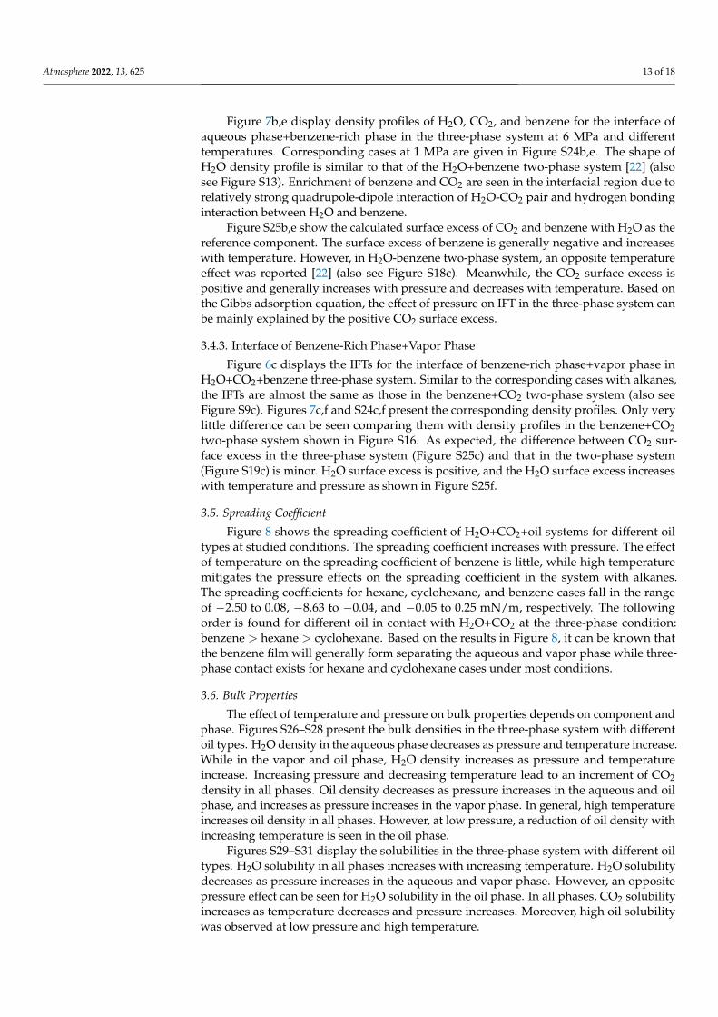
Figure 8 shows the spreading coefficient of H2O+CO2+oil systems for different oiltypes at studied conditions. The spreading coefficient increases with pressure. The effectof temperature on the spreading coefficient of benzene is little, while high temperaturemitigates the pressure effects on the spreading coefficient in the system with alkanes.The spreading coefficients for hexane, cyclohexane, and benzene cases fall in the rangeof −2.50 to 0.08, −8.63 to −0.04, and −0.05 to 0.25 mN/m, respectively. The followingorder is found for different oil in contact with H2O+CO2 at the three-phase condition:benzene > hexane > cyclohexane. Based on the results in Figure 8, it can be known thatthe benzene film will generally form separating the aqueous and vapor phase while three-phase contact exists for hexane and cyclohexane cases under most conditions.

3.6. Bulk Properties

The effect of temperature and pressure on bulk properties depends on component andphase. Figures S26–S28 present the bulk densities in the three-phase system with differentoil types. H2O density in the aqueous phase decreases as pressure and temperature increase.While in the vapor and oil phase, H2O density increases as pressure and temperatureincrease. Increasing pressure and decreasing temperature lead to an increment of CO2density in all phases. Oil density decreases as pressure increases in the aqueous and oilphase, and increases as pressure increases in the vapor phase. In general, high temperatureincreases oil density in all phases. However, at low pressure, a reduction of oil density withincreasing temperature is seen in the oil phase.

Figures S29–S31 display the solubilities in the three-phase system with different oiltypes. H2O solubility in all phases increases with increasing temperature. H2O solubilitydecreases as pressure increases in the aqueous and vapor phase. However, an oppositepressure effect can be seen for H2O solubility in the oil phase. In all phases, CO2 solubilityincreases as temperature decreases and pressure increases. Moreover, high oil solubilitywas observed at low pressure and high temperature.

Atmosphere 2022, 13, 625 14 of 18

Figure 8. Spreading coefficient as a function of pressure in H2O+CO2+oil three-phase systems withdifferent oil: (a) hexane; (b) cyclohexane; (c) benzene.

4. Conclusions

In this study, density gradient theory calculations coupled with PC-SAFT EoS hadbeen carried out to study the interfacial properties in H2O+CO2+oil (hexane, cyclohexane,and benzene) three-phase systems at different temperatures (323, 373, and 423 K) andpressures (1–10 MPa). Generally, the IFTs in three-phase systems decreased with increasingpressure. The reduction of IFT due to pressure increment was more significant at lowertemperature. Other important findings were as follows:

• The IFTs of the aqueous phase+vapor phase in H2O+CO2+oil three-phase systemswere smaller than the IFTs in H2O+CO2 two-phase systems, which could be explainedby enrichment of oil in the interfacial region. The difference between IFTs of aqueousphase+vapor phase in the three-phase system and IFTs in H2O+CO2 two-phase systemwas largest in benzene case and smallest in cyclohexane case due to different degreesof oil enrichment in the interface.

• Significant CO2 enrichment was observed in the interfacial region of the aqueousphase+oil-rich phase in H2O+CO2+oil three-phase systems. This led to the reductionof IFT with increasing pressure while different pressure effects were observed in the

Atmosphere 2022, 13, 625 15 of 18

H2O+oil two-phase systems. The effect of CO2 on the IFTs of aqueous phase+benzene-rich phase interface was small in contrast to that on the IFTs of aqueous phase+alkane(hexane or cyclohexane)-rich phase interface.

• The IFTs of oil-rich phase+vapor phase in H2O+CO2+oil three-phase systems werehardly affected by H2O because of low H2O solubilities in oil and vapor phases.Nevertheless, H2O surface excesses were positive.

• On most conditions, benzene film formed and separated the H2O phase and va-por phase while three-phase contact existed in hexane and cyclohexane cases. Thespreading coefficients of H2O+CO2 in the presence of different oil under three-phaseconditions followed this sequence: benzene > hexane > cyclohexane.

This study provides a fundamental understanding of the interfacial properties of theH2O+CO2+oil three-phase systems. We believe it could help optimize CO2 near-miscibleand immiscible flooding techniques.

Supplementary Materials: The following supporting information can be downloaded at: https://www.mdpi.com/article/10.3390/atmos13040625/s1, Figure S1: Densities of H2O as a function ofpressure at different temperatures. The experimental data from NIST accessed on 6 April 2022(http://webbook.nist.gov/chemistry/fluid) are shown as solid symbols; Figure S2: Densities ofCO2 as a function of pressure at different temperatures. The experimental data from NIST (http://webbook.nist.gov/chemistry/fluid, accessed on 6 April 2022) are shown as solid symbols; Figure S3:Densities of oil as a function of pressure at different temperatures. The experimental data fromNIST (http://webbook.nist.gov/chemistry/fluid, accessed on 6 April 2022) are shown as solidsymbols; Figure S4: Solubilities in H2O+CO2 two-phase system. The experimental data is takenfrom (J. Supercrit. Fluids, 2013, 73: 87–96); Figure S5: Solubilities in H2O+oil two-phase system. Theexperimental data is taken from (J. Phys. Chem. Ref. Data, 2004, 33(2): 549–577) and (J. Chem. Eng.Data, 2003, 48(3): 750–752); Figure S6: Solubilities in oil+CO2 two-phase system. The experimentaldata is taken from (Fluid Phase Equilib., 1987, 33(1–2): 109–123), (J. Chem. Eng. Data, 1987, 32(3):369–371), and (Fluid Phase Equilib., 1987, 36: 107–119); Figure S7: Pressure dependence of IFT inwater-CO2 two-phase system. The experimental data (J. Chem. Thermodyn., 2016, 93: 404) are shownas solid symbols; Figure S8: Pressure dependence of IFT in water+oil two-phase systems: (a) hexane;(b) cyclohexane; (c) benzene. The experimental data (J. Chem. Eng. Data, 1996, 41: 493; J. Phys. Chem.,1951, 55: 439; J. Colloid Interface Sci., 1967, 24: 323) are shown as solid symbols; Figure S9: Pressuredependence of IFT in oil+methane two-phase systems: (a) hexane; (b) cyclohexane; (c) benzene. Theexperimental data (Chin. J. Chem. Eng., 2014, 22: 1302; J Supercrit Fluids, 2019, 154: 104625) are shownas solid symbols; Figure S10: Equilibrium distributions of different species in water+CO2 two-phasesystem at (a) 323 K and 1 MPa, (b) 423 K and 1 MPa, (c) 323 K and 6 MPa, and (d) 423 K and 6 MPa.The solid and dashed lines denote water and CO2, respectively; Figure S11: Equilibrium distributionsof different species in hexane+water two-phase system at (a) 323 K and 1 MPa, (b) 423 K and 1 MPa,(c) 323 K and 6 MPa, and (d) 423 K and 6 MPa. The solid and dashed lines denote water and hexane,respectively; Figure S12: Equilibrium distributions of different species in cyclohexane+water two-phase system at (a) 323 K and 1 MPa, (b) 423 K and 1 MPa, (c) 323 K and 6 MPa, and (d) 423 Kand 6 MPa. The solid and dashed lines denote water and cyclohexane, respectively; Figure S13:Equilibrium distributions of different species in benzene+water two-phase system at (a) 323 K and1 MPa, (b) 423 K and 1 MPa, (c) 323 K and 6 MPa, and (d) 423 K and 6 MPa. The solid and dashedlines denote water and benzene, respectively; Figure S14: Equilibrium distributions of differentspecies in hexane+CO2 two-phase system at (a) 323 K and 1 MPa, (b) 423 K and 1 MPa, (c) 323 K and6 MPa, and (d) 423 K and 6 MPa. The solid and dashed lines denote hexane and CO2, respectively;Figure S15: Equilibrium distributions of different species in cyclohexane+CO2 two-phase system at(a) 323 K and 1 MPa, (b) 423 K and 1 MPa, (c) 323 K and 6 MPa, and (d) 423 K and 6 MPa. The solidand dashed lines denote cyclohexane and CO2, respectively; Figure S16: Equilibrium distributions ofdifferent species in benzene+CO2 two-phase system at (a) 323 K and 1 MPa, (b) 423 K and 1 MPa,(c) 323 K and 6 MPa, and (d) 423 K and 6 MPa. The solid and dashed lines denote benzene and CO2,respectively; Figure S17: Pressure dependence of CO2 surface excess in water+CO2 two-phase system;Figure S18: Pressure dependence of oil surface excess in water+oil two-phase systems: (a) hexane;(b) cyclohexane; (c) benzene; Figure S19: Pressure dependence of CO2 surface excess in oil+CO2two-phase systems: (a) hexane; (b) cyclohexane; (c) benzene; Figure S20: Same as Figure 3, but at

Atmosphere 2022, 13, 625 16 of 18

1 MPa; Figure S21: Pressure dependence of component surface excess in H2O+CO2+hexane three-phase system: (a,d) interface of aqueous phase +vapor phase (top panels); (b,e) interface of aqueousphase+hexane-rich phase (middle panels); (c,f) interface of hexane-rich phase+vapor phase (bottompanels); Figure S22: Same as Figure 5, but at 1 MPa; Figure S23: Pressure dependence of componentsurface excess in H2O+CO2+cyclohexane three-phase system: (a,d) interface of aqueous phase+vapor phase (top panels); (b,e) interface of aqueous phase+cyclohexane-rich phase (middle panels);(c,f) interface of cyclohexane-rich phase+vapor phase (bottom panels); Figure S24: Same as Figure 7,but at 1 MPa; Figure S25: Pressure dependence of component surface excess in H2O+CO2+benzenethree-phase system: (a,d) interface of aqueous phase +vapor phase (top panels); (b,e) interface ofaqueous phase+benzene-rich phase (middle panels); (c,f) interface of benzene-rich phase+vaporphase (bottom panels); Figure S26: Densities in H2O+CO2+hexane three-phase system. Top panelsgive densities in aqueous phase. Middle panels give densities in vapor phase. Bottom panels givedensities in oil phase; Figure S27: Densities in H2O+CO2+cyclohexane three-phase system. Toppanels give densities in aqueous phase. Middle panels give densities in vapor phase. Bottom panelsgive densities in oil phase; Figure S28: Densities in H2O+CO2+benzene three-phase system. Toppanels give densities in aqueous phase. Middle panels give densities in vapor phase. Bottom panelsgive densities in oil phase; Figure S29: Solublities in H2O+CO2+hexane three-phase system. Toppanels give solublities in aqueous phase. Middle panels give solublities in vapor phase. Bottompanels give solublities in oil phase; Figure S30: Solublities in H2O+CO2+cyclohexane three-phasesystem. Top panels give solublities in aqueous phase. Middle panels give solublities in vapor phase.Bottom panels give solublities in oil phase; Figure S31: Solublities in H2O+CO2+benzene three-phasesystem. Top panels give solublities in aqueous phase. Middle panels give solublities in vapor phase.Bottom panels give solublities in oil phase.

Author Contributions: Conceptualization, Y.Y.; methodology, Y.Y.; software, Y.Y.; validation, Y.Y.;formal analysis, Y.Y.; investigation, Y.Y.; resources, Y.Y.; data curation, Y.Y.; writing—original draftpreparation, Y.Y.; writing—review and editing, Y.Y., W.Z., Y.J., T.W. and G.Z.; funding acquisition,Y.Y., T.W. and G.Z. All authors have read and agreed to the published version of the manuscript.

Funding: This research was funded by China University of Mining and Technology grant number102521155. Supported by open fund of State Key Laboratory of Coal Mining and Clean Utilization(China Coal Research Institute) (Grant No. 2021-CMCU-KF019).

Institutional Review Board Statement: Not applicable.

Informed Consent Statement: Not applicable.

Data Availability Statement: Not applicable.

Conflicts of Interest: The authors declare no conflict of interest.

References1. Geden, O. An actionable climate target. Nat. Geosci. 2016, 9, 340–342. [CrossRef]2. Rogelj, J.; Schaeffer, M.; Meinshausen, M.; Knutti, R.; Alcamo, J.; Riahi, K.; Hare, W. Zero emission targets as long-term global

goals for climate protection. Environ. Res. Lett. 2015, 10, 105007. [CrossRef]3. Rogelj, J.; Geden, O.; Cowie, A.; Reisinger, A. Three ways to improve net-zero emissions targets. Nature 2021, 591, 365–368.

[CrossRef] [PubMed]4. Smit, B.; Reimer, J.A.; Oldenburg, C.M.; Bourg, I.C. Introduction to Carbon Capture and Sequestration; World Scientific: Singapore,

2014; Volume 1.5. Wei, J.; Zhou, J.; Li, J.; Zhou, X.; Dong, W.; Cheng, Z. Experimental study on oil recovery mechanism of CO2 associated enhancing

oil recovery methods in low permeability reservoirs. J. Pet. Sci. Eng. 2021, 197, 108047. [CrossRef]6. Ettehadtavakkol, A.; Lake, L.W.; Bryant, S.L. CO2-EOR and storage design optimization. Int. J. Greenh. Gas Control 2014, 25, 79–92.

[CrossRef]7. Zhang, N.; Wei, M.; Bai, B. Statistical and analytical review of worldwide CO2 immiscible field applications. Fuel 2018, 220, 89–100.

[CrossRef]8. Gozalpour, F.; Ren, S.R.; Tohidi, B. CO2 EOR and storage in oil reservoir. Oil Gas Sci. Technol. 2005, 60, 537–546. [CrossRef]9. Deng, X.; Tariq, Z.; Murtaza, M.; Patil, S.; Mahmoud, M.; Kamal, M.S. Relative contribution of wettability Alteration and

interfacial tension reduction in EOR: A critical review. J. Mol. Liq. 2021, 325, 115175. [CrossRef]10. Pereira, L.M.; Chapoy, A.; Burgass, R.; Oliveira, M.B.; Coutinho, J.A.; Tohidi, B. Study of the impact of high temperatures and

pressures on the equilibrium densities and interfacial tension of the carbon dioxide/water system. J. Chem. Thermodyn. 2016,93, 404–415. [CrossRef]

Atmosphere 2022, 13, 625 17 of 18

11. Cai, B.Y.; Yang, J.T.; Guo, T.M. Interfacial tension of hydrocarbon+ water/brine systems under high pressure. J. Chem. Eng. Data1996, 41, 493–496. [CrossRef]

12. Rose, W.E.; Seyer, W.F. The Interfacial Tension of Some Hydrocarbons against Water. J. Phys. Chem. 1951, 55, 439–447. [CrossRef][PubMed]

13. Jennings, H.Y., Jr. The effect of temperature and pressure on the interfacial tension of benzene-water and normal decane-water.J. Colloid Interface Sci. 1967, 24, 323–329. [CrossRef]

14. Yang, Z.; Li, M.; Peng, B.; Lin, M.; Dong, Z.; Ling, Y. Interfacial tension of CO2 and organic liquid under high pressure andtemperature. Chin. J. Chem. Eng. 2014, 22, 1302–1306. [CrossRef]

15. Li, N.; Zhang, C.; Ma, Q.; Sun, Z.; Chen, Y.; Jia, S.; Chen, G.; Sun, C.; Yang, L. Measurements and modeling of interfacial tensionfor (CO2+ n-alkyl benzene) binary mixtures. J. Supercrit. Fluids 2019, 154, 104625. [CrossRef]

16. Nielsen, L.C.; Bourg, I.C.; Sposito, G. Predicting CO2–water interfacial tension under pressure and temperature conditions ofgeologic CO2 storage. Geochim. Cosmochim. Acta 2012, 81, 28–38. [CrossRef]

17. Garrido, J.M.; Quinteros-Lama, H.; Míguez, J.M.; Blas, F.J.; Piñeiro, M.M. On the physical insight into the barotropic effect in theinterfacial behavior for the H2O+ CO2 mixture. J. Phys. Chem. C 2019, 123, 28123–28130. [CrossRef]

18. Choudhary, N.; Che Ruslan, M.F.A.; Narayanan Nair, A.K.; Sun, S. Bulk and interfacial properties of alkanes in the presence ofcarbon dioxide, methane, and their mixture. Ind. Eng. Chem. Res. 2020, 60, 729–738. [CrossRef]

19. Liu, B.; Shi, J.; Wang, M.; Zhang, J.; Sun, B.; Shen, Y.; Sun, X. Reduction in interfacial tension of water–oil interface by supercriticalCO2 in enhanced oil recovery processes studied with molecular dynamics simulation. J. Supercrit. Fluids 2016, 111, 171–178.[CrossRef]

20. Yang, Y.; Narayanan Nair, A.K.; Sun, S. Molecular dynamics simulation study of carbon dioxide, methane, and their mixture inthe presence of brine. J. Phys. Chem. B 2017, 121, 9688–9698. [CrossRef]

21. Yang, Y.; Nair, A.K.N.; Ruslan, M.F.A.C.; Sun, S. Interfacial properties of the alkane+water system in the presence of carbondioxide and hydrophobic silica. Fuel 2022, 310, 122332. [CrossRef]

22. Yang, Y.; Nair, A.K.N.; Ruslan, M.F.A.C.; Sun, S. Interfacial properties of the aromatic hydrocarbon+water system in the presenceof hydrophilic silica. J. Mol. Liq. 2022, 346, 118272. [CrossRef]

23. Georgiadis, A.; Maitland, G.; Trusler, J.M.; Bismarck, A. Interfacial tension measurements of the (H2O+ n-decane+ CO2) ternarysystem at elevated pressures and temperatures. J. Chem. Eng. Data 2011, 56, 4900–4908. [CrossRef]

24. Yang, Y.; Narayanan Nair, A.K.; Anwari Che Ruslan, M.F.; Sun, S. Bulk and interfacial properties of the decane+water system inthe presence of methane, carbon dioxide, and their mixture. J. Phys. Chem. B 2020, 124, 9556–9569. [CrossRef] [PubMed]

25. Papavasileiou, K.D.; Moultos, O.A.; Economou, I.G. Predictions of water/oil interfacial tension at elevated temperatures andpressures: A molecular dynamics simulation study with biomolecular force fields. Fluid Phase Equilibria 2018, 476, 30–38.[CrossRef]

26. Pereira, L.M.; Chapoy, A.; Burgass, R.; Tohidi, B. Measurement and modelling of high pressure density and interfacial tension of(gas+ n-alkane) binary mixtures. J. Chem. Thermodyn. 2016, 97, 55–69. [CrossRef]

27. Choudhary, N.; AK, N.N.; Sun, S. Bulk and interfacial properties of decane in the presence of carbon dioxide, methane, and theirmixture. Sci. Rep. 2019, 9, 19784. [CrossRef]

28. Bahramian, A.; Danesh, A.; Gozalpour, F.; Tohidi, B.; Todd, A. Vapour–liquid interfacial tension of water and hydrocarbonmixture at high pressure and high temperature conditions. Fluid Phase Equilibria 2007, 252, 66–73. [CrossRef]

29. Pereira, L. Interfacial Tension of Reservoir Fluids: An Integrated Experimental and Modelling Investigation. Ph.D. Thesis,Heriot-Watt University, Edinburgh, UK, 2016.

30. Pereira, L.M.C.; Chapoy, A.; Tohidi, B. Vapor-liquid and liquid-liquid interfacial tension of water and hydrocarbon systems atrepresentative reservoir conditions: Experimental and modelling results. In Proceedings of the SPE Annual Technical Conferenceand Exhibition, Society of Petroleum Engineers, Amsterdam, The Netherlands, 27 October 2014.

31. Amin, R.; Smith, T.N. Interfacial tension and spreading coefficient under reservoir conditions. Fluid Phase Equilibria 1998,142, 231–241. [CrossRef]

32. Yang, Y.; Ruslan, M.F.A.C.; Sun, S. Study of Interfacial Properties of Water+Methane+Oil Three-phase Systems by a SimpleMolecular Simulation Protocol. J. Mol. Liq. 2022, 356, 118951. [CrossRef]

33. Li, S.; Zhang, K.; Jia, N.; Liu, L. Evaluation of four CO2 injection schemes for unlocking oils from low-permeability formationsunder immiscible conditions. Fuel 2018, 234, 814–823. [CrossRef]

34. Chen, H.; Li, B.; Duncan, I.; Elkhider, M.; Liu, X. Empirical correlations for prediction of minimum miscible pressure andnear-miscible pressure interval for oil and CO2 systems. Fuel 2020, 278, 118272. [CrossRef]

35. Breger, I.A. Diagenesis of metabolites and a discussion of the origin of petroleum hydrocarbons. Geochim. Cosmochim. Acta 1960,19, 297–308. [CrossRef]

36. Kissin, Y. Catagenesis of light aromatic compounds in petroleum. Org. Geochem. 1998, 29, 947–962. [CrossRef]37. Hostettler, F.D.; Kvenvolden, K.A. Geochemical changes in crude oil spilled from the Exxon Valdez supertanker into Prince

William Sound, Alaska. Org. Geochem. 1994, 21, 927–936. [CrossRef]38. Gross, J.; Sadowski, G. Perturbed-chain SAFT: An equation of state based on a perturbation theory for chain molecules. Ind. Eng.

Chem. Res. 2001, 40, 1244–1260. [CrossRef]

Atmosphere 2022, 13, 625 18 of 18

39. Gross, J.; Sadowski, G. Application of the perturbed-chain SAFT equation of state to associating systems. Ind. Eng. Chem. Res.2002, 41, 5510–5515. [CrossRef]

40. Tsivintzelis, I.; Kontogeorgis, G.M.; Michelsen, M.L.; Stenby, E.H. Modeling phase equilibria for acid gas mixtures using the CPAequation of state. Part II: Binary mixtures with CO2. Fluid Phase Equilibria 2011, 306, 38–56. [CrossRef]

41. Diamantonis, N.I.; Economou, I.G. Evaluation of statistical associating fluid theory (SAFT) and perturbed chain-SAFT equations ofstate for the calculation of thermodynamic derivative properties of fluids related to carbon capture and sequestration. Energy Fuels2011, 25, 3334–3343. [CrossRef]

42. Perez, A.G.; Coquelet, C.; Paricaud, P.; Chapoy, A. Comparative study of vapour-liquid equilibrium and density modelling ofmixtures related to carbon capture and storage with the SRK, PR, PC-SAFT and SAFT-VR Mie equations of state for industrialuses. Fluid Phase Equilibria 2017, 440, 19–35. [CrossRef]

43. Inomata, H.; Arai, K.; Saito, S. Vapor-liquid equilibria for CO2/hydrocarbon mixtures at elevated temperatures and pressures.Fluid Phase Equilibria 1987, 36, 107–119. [CrossRef]

44. Davis, H.; Scriven, L. Stress and structure in fluid interfaces. Adv. Chem. Phys. 1982, 49, 357–454.45. Davis, H.T. Statistical Mechanics of Phases, Interfaces, and Thin Films; Wiley-VCH: Louisville, KY, USA 1996.46. Cornelisse, P.; Peters, C.; de Swaan Arons, J. Application of the Peng-Robinson equation of state to calculate interfacial tensions

and profiles at vapour-liquid interfaces. Fluid Phase Equilibria 1993, 82, 119–129. [CrossRef]47. Miqueu, C.; Miguez, J.M.; Pineiro, M.M.; Lafitte, T.; Mendiboure, B. Simultaneous application of the gradient theory and Monte

Carlo molecular simulation for the investigation of methane/water interfacial properties. J. Phys. Chem. B 2011, 115, 9618–9625.[CrossRef] [PubMed]

48. Lafitte, T.; Mendiboure, B.; Pineiro, M.M.; Bessieres, D.; Miqueu, C. Interfacial properties of water/CO2: A comprehensivedescription through a gradient theory- SAFT-VR Mie approach. J. Phys. Chem. B 2010, 114, 11110–11116. [CrossRef]

49. Mairhofer, J.; Gross, J. Modeling properties of the one-dimensional vapor-liquid interface: Application of classical densityfunctional and density gradient theory. Fluid Phase Equilibria 2018, 458, 243–252. [CrossRef]

50. Rachford, H.H.; Rice, J. Procedure for use of electronic digital computers in calculating flash vaporization hydrocarbonequilibrium. J. Pet. Technol. 1952, 4, 19. [CrossRef]

51. Mejía, A.; Muller, E.A.; Chaparro Maldonado, G. SGTPy: A Python code for calculating the interfacial properties of fluids basedon the square gradient theory using the SAFT-VR Mie equation of state. J. Chem. Inf. Model. 2021, 61, 1244–1250. [CrossRef]

52. Harkins, W.D.; Feldman, A. Films. The spreading of liquids and the spreading coefficient. J. Am. Chem. Soc. 1922, 44, 2665–2685.[CrossRef]

53. Shaw, D.J. Introduction to Colloid and Surface Chemistry; Butterworths: London, UK, 1980.54. Bonn, D.; Eggers, J.; Indekeu, J.; Meunier, J.; Rolley, E. Wetting and spreading. Rev. Mod. Phys. 2009, 81, 739. [CrossRef]55. Bertrand, E.; Bonn, D.; Meunier, J.; Segal, D. Wetting of alkanes on water. Phys. Rev. Lett. 2001, 86, 3208. [CrossRef]56. Linstrom, P.J.; Mallard, W.G. The NIST Chemistry WebBook: A chemical data resource on the internet. J. Chem. Eng. Data 2001,

46, 1059–1063. [CrossRef]57. Hou, S.X.; Maitland, G.C.; Trusler, J.M. Measurement and modeling of the phase behavior of the (carbon dioxide+ water) mixture

at temperatures from 298.15 K to 448.15 K. J. Supercrit. Fluids 2013, 73, 87–96. [CrossRef]58. Maczynski, A.; Wisniewska-Gocłowska, B.; Góral, M. Recommended liquid–liquid equilibrium data. Part 1. Binary alkane–water

systems. J. Phys. Chem. Ref. Data 2004, 33, 549–577. [CrossRef]59. Jou, F.Y.; Mather, A.E. Liquid- liquid equilibria for binary mixtures of water+ benzene, water+ toluene, and water+ p-xylene from

273 K to 458 K. J. Chem. Eng. Data 2003, 48, 750–752. [CrossRef]60. Wagner, Z.; Wichterle, I. High-pressure vapour—liquid equilibrium in systems containing carbon dioxide, 1-hexene, and n-hexane.

Fluid Phase Equilibria 1987, 33, 109–123. [CrossRef]61. Nagarajan, N.; Robinson, R., Jr. Equilibrium phase compositions, phase densities, and interfacial tensions for carbon dioxide+

hydrocarbon systems. 3. CO2+ cyclohexane. 4. CO2+ benzene. J. Chem. Eng. Data 1987, 32, 369–371. [CrossRef]62. Yang, Y.; Che Ruslan, M.F.A.; Narayanan Nair, A.K.; Sun, S. Effect of ion valency on the properties of the carbon dioxide–methane–

brine system. J. Phys. Chem. B 2019, 123, 2719–2727. [CrossRef]63. Stephan, S.; Hasse, H. Enrichment at vapour–liquid interfaces of mixtures: Establishing a link between nanoscopic and

macroscopic properties. Int. Rev. Phys. Chem. 2020, 39, 319–349. [CrossRef]64. Li, X.; Ross, D.A.; Trusler, J.M.; Maitland, G.C.; Boek, E.S. Molecular dynamics simulations of CO2 and brine interfacial tension at

high temperatures and pressures. J. Phys. Chem. B 2013, 117, 5647–5652. [CrossRef]65. Feller, D. Strength of the benzene- water hydrogen bond. J. Phys. Chem. A 1999, 103, 7558–7561. [CrossRef]