Complex Variables and Elliptic Equations, 2013

Vol. 58, No. 3, 415–430, http://dx.doi.org/10.1080/17476933.2011.593097

Schrodinger type equations with real-time variable and

complex spatial variables

Ciprian G. Gala*, Sorin G. Galb and Jerome A. Goldsteinc

aDepartment of Mathematical Sciences, The University of Missouri, Columbia,MO 65211, USA; bDepartment of Mathematics and Computer Science,University of Oradea, Str. Universitatii Nr. 1, 410087 Oradea, Romania;

cDepartment of Mathematical Sciences, The University of Memphis,Memphis, TN 38152, USA

Communicated by V. Radulescu

(Received 23 February 2011; final version received 27 May 2011)

In recent work, heat and Laplace equations, (un)damped wave equations,the Burgers and the Black–Merton–Scholes equations with real-timevariable and complex spatial variable were studied. The purpose of thisarticle is to make a similar study for the Schrodinger equation withreal-time variable and complex spatial variable. The complexification of thespatial variable in the case of the Schrodinger equation is made by twodifferent methods which produce different equations: first, one complexifiesthe spatial variable in the corresponding convolution formula by replacingthe usual sum of variables (translation) by an exponential product(rotation) and second, one complexifies the spatial variable in thecorresponding evolution equation and then one searches for non-analyticand for analytic solutions. By both methods, new kinds of evolutionequations (or systems of equations) in two-dimensional spatial variables aregenerated and their solutions are constructed. It is of interest to note that inthe case of the first method, solutions can be studied by employing thepowerful theory of groups of linear operators. Then, we show that thesesolutions preserve some geometric properties of the boundary function, likethe univalence, starlikeness, convexity and spirallikeness. In the case of thehigher order Schrodinger equation, the complexification of the spatialvariable is made in the corresponding convolution formula.

Keywords: Schrodinger equation; higher order Schrodinger equation;complex convolution integrals; complex spatial variables; groups of linearoperators on locally convex spaces; univalence; starlikeness; convexity;spirallikeness

AMS Subject Classifications: 47D03; 47D06; 47D60; 30C45

*Corresponding author. Email: galc@missouri.edu

� 2013 Taylor & Francis

Dow

nloa

ded

by [

Flor

ida

Inte

rnat

iona

l Uni

vers

ity]

at 1

1:27

21

May

201

5

1. Introduction

Let us consider the Cauchy problem for the case of the one-dimensional Schrodingerequation

i@u

@tðt, xÞ þ

@2u

@x2ðt, xÞ ¼ 0, ðt, xÞ 2R�R,

uð0, xÞ ¼ f ðxÞ, x2R,

8<: ð1:1Þ

where f and u are complex-valued functions. It is well-known that under certainconditions, such as f2L1(R),

uðt, xÞ ¼1ffiffiffiffiffiffiffiffiffi4�itp

Z þ1�1

f ðx� uÞeiu2=ð4tÞdu ð1:2Þ

is a solution of the above initial value problem (see, e.g. [1]). In other spaces, likeL2(R), it is also the unique solution. In particular, the integral operator in (1.2)defines a group of isometries in the space L2(R).

It is natural to ask what happens if in the Schrodinger equation we complexifythe spatial variable and keep the time variable real? It is the goal of this article toanswer this question. To the best of our knowledge, it is the first time when such astudy is made. This will be done for the Schrodinger equation in Section 2 and for itshigher order version in Section 3. This topic was already developed in detail forcomplex heat and Laplace equations in [2,3], and complex wave and telegraphequations in [4]. Finally in [5], the Burgers and Black–Merton–Scholes equationswith real-time variable and complex spatial variable were also analyzed.

The complexification of the spatial variable in the Schrodinger equation is madeby two different methods which produce different equations: first, one complexifiesthe spatial variable in the corresponding formula (1.2) by replacing the usual sum ofvariables (translation) by an exponential product(rotation). We will then establishthat the resulting operator defines a (C0)-group of linear operators which is locallyequicontinuous on some locally convex space A(DR), for a discDR of radius R41.This method yields solutions that satisfy proper differential equations, and whichpreserve some geometric properties of the boundary function, such as, univalence,starlikeness, convexity and spirallikeness. Second, one directly complexifies thespatial variable in the corresponding evolution equation of (1.1), and then onesearches for analytic and non-analytic solutions for the resulting equation.

The plan of this article is as follows. Section 2 treats the case of the complexifiedSchrodinger equation, while Section 3 deals with the complexification of its higherorder version. For future study, we note that it would be plausible to seekcomparable results for regions other than the open unit discD and for otheroperators similar to the Laplacian D.

2. Schrodinger equation with complex spatial variable

For R41, let us define the open discDR¼ {z2C; jzj5R}. Let us consider the locallyconvex space

AðDRÞ ¼ f f:DR ! C; f is analytic on DRg,

416 C. G. Gal et al.

Dow

nloa

ded

by [

Flor

ida

Inte

rnat

iona

l Uni

vers

ity]

at 1

1:27

21

May

201

5

endowed with the countable family of seminorms generated by a sequence Rn%R,

Rn� 1, for all n2N, given by

k f kn ¼ supfj f ðzÞj; z2DRng:

It is well-known that, when the space A(DR) is endowed with the metric

dð f, gÞ ¼X1n¼0

1

2nk f� gkn

1þ k f� gkn,

we have that A(DR) is a Frechet space.For f2A(DR), we will complexify the integral solution (1.2), by replacing the

usual translations x� u2R in (1.2) with the rotations ze�iu2C. To this end, we

define

uðt, zÞ ¼1ffiffiffiffiffiffiffiffiffi4�itp

Z þ1�1

f ðze�iuÞeiu2=ð4tÞdu, z2DR, t2Rnf0g: ð2:1Þ

We aim to study this complex convolution integral (2.1) by showing that, for analytic

functions f2A(DR), the function u, defined by (2.1), satisfies a proper differential

equation in DR.

THEOREM 2.1 Let R41 and f2A(DR), that is, f ðzÞ ¼P1

k¼0 akzk, for all z2DR.

(i) For all t2R\{0}, u(t, z), defined by (2.1) is analytic in DR, and we have on DR:

uðt, zÞ ¼X1k¼0

ake�ik2tzk:

Also, we have u(0, z)¼ f(z), for all z2DR.(ii) For all z2Dr with 1� r5R and t2R, the following estimate holds:

juðt, zÞ � f ðzÞj �t2

2

X1k¼0

jakjk4rk þ jtj

X1k¼0

jakjk2rk,

whereP1

k¼0 jakjk4rk 51, from f(4)2A(DR).

(iii) For all z2Dr with 1� r5R and t, s2R, we have:

juðt, zÞ � uðs, zÞj � 2X1k¼0

jakjk2rkjt� sj:

(iv) Denoting T(t)( f )(z)¼ u(t, z), where u(t, z) is given by (2.1), then {T(t)}t2R is a

(C0)-group of linear operators, locally equicontinuous (that is equicontinuous

for t2 [�a, a], with some a40) on the locally convex space A(DR), and the

unique solution of the Cauchy problem

i@u

@tðt, zÞ þ

@2u

@’2ðt, zÞ ¼ 0, ðt, zÞ 2R�DR, z ¼ rei’, 05 r5R, z 6¼ 0, ð2:2Þ

uð0, zÞ ¼ f ðzÞ, z2DR, f2AðDRÞ: ð2:3Þ

Moreover, u(t, z) belongs to A(DR), for each fixed t.

Complex Variables and Elliptic Equations 417

Dow

nloa

ded

by [

Flor

ida

Inte

rnat

iona

l Uni

vers

ity]

at 1

1:27

21

May

201

5

Proof (i) For fixed z2DR, we get f ðze�iuÞ ¼P1

k¼0 ake�ikuzk: Since jake

�ikuj ¼ jakj,

for all u2R, and sinceP1

k¼0 akzk is absolutely convergent, it follows thatP1

k¼0 ake�ikuzk is uniformly convergent with respect to u2R. This immediately

implies that the series can be integrated term by term, that is,

uðt, zÞ ¼1ffiffiffiffiffiffiffiffiffi4�itp

X1k¼0

akzk

Z 1�1

e�ikueiu2=ð4tÞdu

� �

¼1ffiffiffiffiffiffiffiffiffi4�itp

X1k¼0

akzk

Z 1�1

cos ku�u2

4t

� �duþ i

Z 1�1

sinu2

4t� ku

� �du

� �:

Suppose now that t40. Writing ku� u2

4t ¼ k2t��u�2kt2ffiffitp�2

and making the followingchange of variable v ¼ u�2kt

2ffiffitp , we easily deduceZ 1

�1

cos ku�u2

4t

� �du

¼ cosðk2tÞ

Z 1�1

cosu� 2kt

2ffiffitp

� �2" #

duþ sinðk2tÞ

Z 1�1

sinu� 2kt

2ffiffitp

� �2" #

du

¼ 2ffiffitp

cosðk2tÞ

Z 1�1

cosðv2Þdvþ 2ffiffitp

sinðk2tÞ

Z 1�1

sinðv2Þdv

¼ffiffiffiffiffiffiffi2�tp

cosðk2tÞ þ sinðk2tÞ

:

Here we have used the well-known values of the Fresnel integrals (see, e.g.[6, Chapter 7]), Z 1

�1

cosðv2Þdv ¼

Z 1�1

sinðv2Þdv ¼

ffiffiffiffiffiffi2�p

2:

Analogously, we haveZ 1�1

sinu2

4t� ku

� �du

¼ cosðk2tÞ

Z 1�1

sinu� 2kt

2ffiffitp

� �2" #

du� sinðk2tÞ

Z 1�1

cosu� 2kt

2ffiffitp

� �2" #

du

¼ffiffiffiffiffiffiffi2�tp

cosðk2tÞ � sinðk2tÞ

:

On account of the last two identities, we get

uðt, zÞ ¼1ffiffiffiffiffiffiffiffiffi4�itp

X1k¼0

akzkffiffiffiffiffiffiffi2�tp

½e�ik2t þ ie�ik

2t�

¼1ffiffiffiffiffiffiffiffiffi4�itp

X1k¼0

akzkð1þ iÞ

ffiffiffiffiffiffiffi2�tp

e�ik2t

¼X1k¼0

akzke�ik

2t,

where we have used the fact thatffiffiip¼ ei�=4 ¼ cosð�=4Þ þ i sinð�=4Þ ¼

ffiffi2p

2 ð1þ iÞ. Thisproves (i), for positive times.

418 C. G. Gal et al.

Dow

nloa

ded

by [

Flor

ida

Inte

rnat

iona

l Uni

vers

ity]

at 1

1:27

21

May

201

5

Suppose now that t50. In this case, taking into account that cos(�) (and sin(�),

respectively) is an even (odd, respectively) function, by making a simple change of

variable v ¼ u�2kt2ffiffiffiffi�tp , we can getZ 1

�1

cos ku�u2

4t

� �du

¼ cosðk2tÞ

Z 1�1

cosu� 2kt

2ffiffiffiffiffiffi�tp

� �2" #

du� sinðk2tÞ

Z 1�1

sinu� 2kt

2ffiffiffiffiffiffi�tp

� �2" #

du

¼ 2ffiffiffiffiffiffi�tp

cosðk2tÞ

Z 1�1

cosðv2Þdv� 2ffiffiffiffiffiffi�tp

sinðk2tÞ

Z 1�1

sinðv2Þdv

¼ffiffiffiffiffiffiffiffiffiffiffiffiffiffi2�ð�tÞ

pcosðk2tÞ � sinðk2tÞ

:

Analogously, we haveZ 1�1

sinu2

4t� ku

� �du

¼ � cosðk2tÞ

Z 1�1

sinu� 2kt

2ffiffiffiffiffiffi�tp

� �2" #

du� sinðk2tÞ

Z 1�1

cosu� 2kt

2ffiffiffiffiffiffi�tp

� �2" #

du

¼ffiffiffiffiffiffiffiffiffiffiffiffiffiffi2�ð�tÞ

p� cosðk2tÞ � sinðk2tÞ

:

Thus, we get

uðt, zÞ ¼1ffiffiffiffiffiffiffiffiffi4�itp

X1k¼0

akzkffiffiffiffiffiffiffiffiffiffiffiffiffiffi2�ð�tÞ

p½e�ik

2t � ie�ik2t�

¼1ffiffiffiffiffiffiffiffiffi4�itp

X1k¼0

akzkð1� iÞ

ffiffiffiffiffiffiffiffiffiffiffiffiffiffi2�ð�tÞ

pe�ik

2t

¼ð1� iÞ

ffiffiffiffiffiffiffiffiffiffiffiffiffiffi2�ð�tÞ

p2ffiffiffi�p ffiffiffiffiffiffiffiffiffi

ð�iÞp ffiffiffiffiffiffiffiffiffi

ð�tÞp ¼

X1k¼0

akzke�ik

2t,

where we have used the formulaffiffiffiffiffiffi�ip¼ e

12ði argð�iÞÞ ¼ e�i�=4 ¼ cosð�=4Þ�

i sinð�=4Þ ¼ffiffi2p

2 ð1� iÞ. This proves (i), for negative times.(ii) Let jzj � r. We obtain

juðt, zÞ � f ðzÞj ¼X1k¼0

akzk½e�ik

2t � 1�

����������

¼X1k¼0

akzk½�2 sin2ðk2t=2Þ þ i sinðk2t=2Þ � cosðk2t=2Þ�

����������

�X1k¼0

jakjrkj2 sin2ðk2t=2Þj þ

X1k¼0

jakjrkj2 sinðk2t=2Þj

�t2

2

X1k¼0

jakjk4rk þ jtj

X1k¼0

jakjk2rk,

since jsin(x)j � jxj, for all x2R.

Complex Variables and Elliptic Equations 419

Dow

nloa

ded

by [

Flor

ida

Inte

rnat

iona

l Uni

vers

ity]

at 1

1:27

21

May

201

5

(iii) We have

juðt, zÞ � uðt, sÞj ¼X1k¼0

akzk½e�ik

2t � e�ik2s�

����������

¼X1k¼0

½cosðk2tÞ � cosðk2sÞ � iðsinðk2tÞ � sinðk2sÞÞ�

¼X1k¼0

akzk �2 sin k2ðtþ sÞ=2

� �sin k2ðt� sÞ=2� �������

�2i sin k2ðt� sÞ=2� �

cos k2ðtþ sÞ=2� � ��

� 4X1k¼0

jakjrk sin

k2ðt� sÞ

2

� ��������� � 2

X1k¼0

jakjk2rkjt� sj:

(iv) From (i), it is immediate that T(tþ s)¼T(t)(T(s)), for all t, s2R; using (ii),we easily get that T(0)¼ I. The strong continuity of T(�) follows from (iii). Inparticular, according to, e.g. [7, p. 232], (T(t))t2R is a C0-group of linear operators onA(DR). Since A(DR) is a Frechet space, it follows that (T(t))t2R is also locallyequicontinuous (see, e.g. [8,9]). For f2A(DR) such that f ðzÞ ¼

P1k¼0 akz

k, z2DR,z¼ rei’, z 6¼ 0, r5R, on account of (i), we can now write

TðtÞð f ÞðzÞ ¼X1k¼0

ake�ik2trkeki’:

Since this series is uniformly convergent in any compact disc included in DR, it can bedifferentiated term by term, with respect to t and ’. We then easily obtain thatT(t)( f )(z) satisfies (2.2) for all z2DR. Note that the generator of this group T(t),t2R, can be computed explicitly,

Gð f ÞðzÞ ¼d½TðtÞð f ÞðzÞ�

dtjt¼0 ¼ �i

X1k¼0

k2akzk ¼ i

@2TðtÞð f ÞðzÞ

@’2:

Also, using the same series representation, it is easy to check that

Tð0Þð f ÞðzÞ ¼ f ðzÞ, z2DR:

Finally, reasoning now exactly as in [10, Theorem 1.2, p. 83], it follows thatu(t, z)¼T(t)( f )(z) is the unique solution of the Cauchy problem (2.2)–(2.3). We alsonote that, in (2.2) we must take z 6¼ 0 simply because z¼ 0 has no polarrepresentation, that is, z¼ 0 cannot be represented as function of ’. This completesthe proof of the theorem. g

The next result shows that the solution of problem (2.2)–(2.3) preserves someinteresting geometric properties on the unit disc, of the boundary function. In orderto state these properties more precisely, we need to consider some definitions for thefollowing well-known subclasses of univalent analytic functions:

S�ðD1Þ ¼

(f2AðD1Þ; f ð0Þ ¼ f 0ð0Þ � 1 ¼ 0,Re

zf 0ðzÞ

f ðzÞ

� �4 0, for all z2D1

),

420 C. G. Gal et al.

Dow

nloa

ded

by [

Flor

ida

Inte

rnat

iona

l Uni

vers

ity]

at 1

1:27

21

May

201

5

S��ðD1Þ ¼

(f2AðD1Þ; fð0Þ¼ f 0ð0Þ�1¼ 0,Re ei�

zf 0ðzÞ

fðzÞ

� �40, for all z2D1

), j�j5�=2,

KðD1Þ ¼

(f2AðD1Þ; f ð0Þ ¼ f 0ð0Þ � 1 ¼ 0,Re

zf 00ðzÞ

f 0ðzÞþ 1

� �4 0, for all z2D1

),

S2ðD1Þ ¼

(f2AðD1Þ; f ðzÞ ¼

X1k¼1

akzk, ja1j �

X1k¼2

jakj

)

and

S1ðD1Þ ¼

�f2AðD1Þ, f ðzÞ ¼ zþ

X1k¼2

akzk,X1k¼2

kjakj � 1

�:

We recall that S�(D1), S��ðD1Þ and K(D1) are called the classes of normalized starlike,

spirallike and convex functions on D1, respectively. According to, e.g. [11, p. 97,

Exercise 4.9.1], if f2S1(D1), then jzf 00(z)/f(z)� 1j51 8z2D1, and therefore f is

starlike (and univalent) on D1. Also, if f2S2(D1), then f is starlike in D1 [12].

THEOREM 2.2 Let u(t, z) be the unique solution of the Cauchy problem (2.2)–(2.3),

given by (2.1). Let f2A(DR) with R41.

(i) As function of z, u(t, z) has the following properties: if f2S1(D1), then

eitu(t, z)2S1(D1), for all t2R\{0} and, if f2S2(D1), then u(t, z)2S2(D1),

for all t2R.(ii) For all t2 [�tf, tf]\{0} with sufficiently small tf40 (depending on f ), the

solution u(t, z) preserves, as function of z, the starlikeness, convexity and

spirallikeness of the boundary function f in D1.

Proof (i) Let t2R\{0} and assume f2S1(D1) such that f ðzÞ ¼ zþP1

k¼2 akzk, withP1

k¼2 kjakj � 1. First, it follows from Theorem 2.1, (i), that eitu(t, 0)¼ 0 and

eit½uðt, zÞ� 0z¼0 ¼ 1. Moreover, we can write

eituðt, zÞ ¼X1k¼0

akeite�ik

2tzk,

and

X1k¼2

kjake�ik2teitj ¼

X1k¼2

kjakj � 1,

which proves that u(t, z)2S1(D1), as function of z.

Now, let f2S2(D1). It follows that a0¼ 0 andP1

k¼2 jakj � ja1j. By Theorem 2.1(i),

we get

uðt, zÞ ¼X1k¼0

ake�ik2tzk ¼

X1k¼1

ake�ik2tzk,

Complex Variables and Elliptic Equations 421

Dow

nloa

ded

by [

Flor

ida

Inte

rnat

iona

l Uni

vers

ity]

at 1

1:27

21

May

201

5

which implies

X1k¼2

jakjje�ik2tj �

X1k¼2

jakj � ja1j ¼ ja1jje�itj,

and, therefore, u2S2(D1).(ii) From Theorem 2.1(i) and (ii), it is readily seen that u(t, z) is analytic in DR

and u(t, z) converges to f(z), as t! 0, uniformly in D1. This convergence together

with an application of a well-known Weierstrass’s result yield that [u(t, z)]0 ! f 0(z)

and [u(t, z)]00 ! f 00(z), uniformly in D1, as t! 0. In what follows, from now on,

Pt( f )(z) will denote u(t, z)/b1(t), where b1(t)¼ a1e�it is the coefficient of z, in the

Taylor series representation of the analytic function u(t, z). We will also denote by

P 0t ð f ÞðzÞ and P 00t ð f ÞðzÞ, the corresponding first- and second-order derivatives of

Pt( f )(z) with respect to z.

If f(0)¼ f 0(0)� 1¼ 0, it is not difficult to observe that b1(t) 6¼ 0, Pt( f )(0)¼ f(0)/

b1(t)¼ 0, P 0t ð f Þð0Þ ¼ uðt, 0Þ 0=b1ðtÞ ¼ 1 and b1(t) converges to f 0(0)¼ 1 as t! 0. This

obviously implies that, for t! 0, we have Pt( f )(z)! f(z), P 0t ð f ÞðzÞ ! f 0ðzÞ and

P 00t ð f ÞðzÞ ! f 00ðzÞ, uniformly in D1. The rest of the proof is identical to the proof of

[2, Theorem 2.2]. g

Remark 2.3 (a) Taking into account the fact that @@’ ¼

@@z �

@z@’ ¼

@@z � ðizÞ and

@2

@’2¼ �z @

@z� z2 @2

@z2, Equation (2.2) is equivalent to

i@u

@tðt, zÞ ¼ z

@u

@zðt, zÞ þ z2

@2u

@z2ðt, zÞ:

(b) Since the constant eit does not influence the starlikeness and the univalence of

u(t, z) in the above result, it follows that for f2S1(D1) and t2R\{0}, the solution of

(2.2)–(2.3) is starlike (and univalent) in D1, as function of z. Moreover, in view of the

Riemann mapping theorem (see, e.g. [13, Chapter I]), all the geometric properties

concerning the solution of problem (2.2)–(2.3), stated by Theorem 2.2, can be readily

translated into statements which hold in any disc of radius r with 1� r5R.

In what follows, the Schrodinger equation is complexified, by replacing x2R

with z2C. More precisely, we aim to study the following initial value problem for a

Schrodinger-type equation

i@u

@tðt, zÞ þ

@2u

@z2ðt, zÞ ¼ 0,

uð0, zÞ ¼ f ðzÞ:

8<: ð2:4Þ

We will first consider the case when f is analytic and our goal is to search for the

analytic solutions u(t, z), as functions of z, for any t2R. In this case, by taking

u(t, z)¼ u1(t, x, y)þ iu2(t, x, y), for z¼ xþ iy, we have @u@z ¼

@u1@x þ i @u2@x and

@2u@z2¼ @2u1

@x2þ i @

2u2@x2

; hence, the initial value problem (2.4) reduces to solving

i@u1@tþ i

@u2@t

� �þ@2u1@x2þ i

@2u2@x2¼ 0,

uð0, zÞ ¼ f ðzÞ:

8<: ð2:5Þ

422 C. G. Gal et al.

Dow

nloa

ded

by [

Flor

ida

Inte

rnat

iona

l Uni

vers

ity]

at 1

1:27

21

May

201

5

Now, setting f(z)¼ f1(x, y)þ if2(x, y), it is immediate that (2.5) is equivalent to the

following system:

@u1@t¼ �

@2u2@x2

,@u2@t¼@2u1@x2

, u1ð0,x, yÞ ¼ f1ðx, yÞ, u2ð0, x, yÞ ¼ f2ðx, yÞ: ð2:6Þ

Since, by hypothesis the couple ( f1, f2) satisfies the Cauchy–Riemann equations with

respect to x and y, we can prove the following result.

THEOREM 2.4 For d40, denote by Sd the strip {z¼ xþ iy; x, y2R, jyj � d}, and

define as L2xðSdÞ, the class of all functions f : Sd!C, f-analytic on Sd, such that if

f(z)¼ f1(x, y)þ if2(x, y), z¼xþ iy2Sd, then f1(x, y), f2(x, y),@f1@x ðx, yÞ,

@f1@y ðx, yÞ,

@f2@x ðx, yÞ,

@f2@y ðx, yÞ are in L2(R), as functions of x, for any fixed jyj � d. Then, for

f2L2xðSdÞ,

uðt, zÞ ¼1ffiffiffiffiffiffiffiffiffi4�itp

Z þ1�1

f ðz� uÞeiu2=ð4tÞdu

is the unique (analytic, as function of z) solution of (2.4), for any t2R\{0}.

Proof For f(z)¼ f1(x, y)þ if2(x, y), we can write

uðt, zÞ ¼1ffiffiffiffiffiffiffiffiffi4�itp

Z þ1�1

f1ðx� u, yÞeiu2=ð4tÞduþ i

1ffiffiffiffiffiffiffiffiffi4�itp

Z þ1�1

f2ðx� u, yÞeiu2=ð4tÞdu

:¼ u1ðt,x, yÞ þ iu2ðt, x, yÞ,

for all z¼ xþ iy2Sd. Translating the initial condition of (2.5) into the initial

conditions of (2.6) for both u1 and u2, and employing a well-known result concerning

problem (1.1), we deduce that for each fixed, arbitrary y, with jyj � d, u1 and u2 are

the unique solutions of the following Cauchy problems

i@u1@tðt, x, yÞ þ

@2u1@x2ðt,x, yÞ ¼ 0, ðt, xÞ 2R� R,

u1ð0,x, yÞ ¼ f1ðx, yÞ, x2R,

8<:

and

i@u2@tðt, xÞ þ

@2u2@x2ðt,xÞ ¼ 0, ðt, xÞ 2R� R,

u2ð0, x, yÞ ¼ f2ðx, yÞ, x2R:

8<:

Thus, it is easy to check that u¼ u1þ iu2 satisfies (2.5), which is equivalent to saying

that u is the unique solution of (2.4).It remains to show that u(�, z) is analytic on Sd. This immediately follows from the

analyticity of f¼ f1þ if2 and the continuity on Sd, of the partial derivatives@f1@x ðx, yÞ,

@f1@y ðx, yÞ,

@f2@x ðx, yÞ,

@f2@y ðx, yÞ. The fact that f2L2

xðSdÞ assures, in addition, that u1, u2exist and that we can differentiate u1 and u2 under the sign of the improper

integrals (for such a criterion, see, e.g. [14, p. 293, Exercise 607]). By the above

considerations, it is easy to check that u1 and u2 satisfy the Cauchy–Riemann

conditions and that they have continuous partial derivatives of first order. This

proves the theorem. g

Complex Variables and Elliptic Equations 423

Dow

nloa

ded

by [

Flor

ida

Inte

rnat

iona

l Uni

vers

ity]

at 1

1:27

21

May

201

5

Remark 2.5 Here, we shall use the opportunity to correct some mistakes concerning

some hypotheses of some results in [2]. A much closer look at the main formulae in

[2, Theorems 2.4 and 3.4], indicates that the boundary function f(z) (and

consequently the solution u(�, z)) need to be defined in a strip that contains the

x-axis and not only in the closed unit disc D as they were in [2, Theorems 2.4

and 3.4]. Moreover, we must also make some corrections in the statements of

[2, Theorems 2.7 and 3.6], where the non-analytic boundary function f(z) (and,

consequently, the corresponding non-analytic solution u(�, z)) has to be defined on

the whole C and not only in the closed unit disc. The statements of these results

remain true even for these minor modifications.

Another natural way of complexification of the Schrodinger equation would be

to replace @2

@x2by @2

@z2þ @2

@z2(since @

@z ¼ 0, for analytic functions). In this case, by

definition we have

@u

@z¼

1

2

@u

@xþ

1

2i

@u

@y,

@u

@z¼

1

2

@u

@x�

1

2i

@u

@y,

and these identities imply

@u

@x¼@u

@zþ@u

@z,

@u

@y¼ i

@u

@z�@u

@z

� �:

We may, formally, write @x ¼ @z þ @z, @y ¼ i @z � @zð Þ. Therefore, we have

@2u

@x2¼@

@x

@u

@x

� �¼ ð@z þ @zÞ

2

and

@2u

@y2¼@

@y

@u

@y

� �¼ ½ið@z � @zÞ�

2,

which immediately implies that

@2u

@z2þ@2u

@z2

� �¼

1

2

@2u

@x2�@2u

@y2

� �:

Consequently, in this case we obtain the following differential equation:

i@u

@tþ1

2

@2u

@x2�@2u

@y2

� �¼ 0:

Replacing now, u(t, z)¼ u1(t, x, y)þ iu2(t, x, y) and f(z)¼ f1(x, y)þ if2(x, y) (assuming

that f1, f22C2), we may obtain the following coupled system of partial differential

equations:

@u1@t¼

1

2

@2u2@y2�@2u2@x2

� �,

@u2@t¼

1

2

@2u1@x2�@2u1@y2

� �, ð2:7Þ

424 C. G. Gal et al.

Dow

nloa

ded

by [

Flor

ida

Inte

rnat

iona

l Uni

vers

ity]

at 1

1:27

21

May

201

5

subject to the initial conditions:

u1ð0, x, yÞ ¼ f1ðx, yÞ, u2ð0,x, yÞ ¼ f2ðx, yÞ, ð2:8Þ

where x2þ y2� 1.Concerning the solutions of (2.7)–(2.8), we present the following result.

THEOREM 2.6 Assuming that f1, f22C1 have all their partial derivatives bounded by

the same constant, a solution U ¼ u1u2

� �of the system (2.7)–(2.8) is given by

U(t)¼ etA(U0), where U0 ¼f1f2

� �, and A is the matrix A¼ (ai, j), i, j¼ 1, 2, with

a1,1 ¼ a2,2 ¼ 0, a1,2 ¼ DH :¼1

2

@2

@y2�@2

@x2

� �, a2,1 ¼ �DH

and

A2n ¼ ðai, jÞ, i, j ¼ 1, 2, a1,2 ¼ a2,1 ¼ 0, a1,1 ¼ ð�1ÞnD2n

H , a2,2 ¼ a1,1, n � 1,

A2n�1 ¼ ðai, jÞ, i, j ¼ 1, 2, a1,1 ¼ a2,2 ¼ 0, a1,2 ¼ ð�1Þn�1D2n�1

H , n � 1,

a2,1 ¼ �a1,2:

Proof The system (2.7)–(2.8) can be rewritten as

dU

dt¼ AU, Uð0Þ ¼

f1f2

� �:¼ U0:

The solution has the form U(t)¼ etA(U0). Finally, the powers An, n2N can be

obtained by simple calculations. g

Now, since @u@z ¼ 0 for any analytic function u, the analytic case can also be

generalized, by replacing @2

@x2with @2

@z2� @2

@z2. In this case, following a similar calculation

as above, we easily deduce

@2

@z2�@2

@z2¼

1

i

@2

@x@y: ð2:9Þ

This immediately leads to the following uncoupled system of evolution equations:

@u1@t¼@2u1@x@y

,@u2@t¼@2u2@x@y

, ð2:10Þ

u1ð0, x, yÞ ¼ f1ðx, yÞ, u2ð0,x, yÞ ¼ f2ðx, yÞ, ð2:11Þ

where x2þ y2� 1.In this case, we have the following result.

THEOREM 2.7 If f1 and f2 have partial derivatives of any order, bounded by the

same constant, then a solution of the problem (2.10)–(2.11) is given by

Complex Variables and Elliptic Equations 425

Dow

nloa

ded

by [

Flor

ida

Inte

rnat

iona

l Uni

vers

ity]

at 1

1:27

21

May

201

5

uj(t,x, y)¼ etL( fj)(x, y), j¼ 1, 2, where LðF Þðx, yÞ :¼ @2F@x@y ðx, yÞ, that is,

ujðt, x, yÞ ¼X1k¼0

tk

k!Lkð fjÞðx, yÞ,

for j¼ 1, 2, all t2R and (x, y)2R2, with x2þ y2� 1.

Proof First, note that the two equations in (2.10) are not coupled. If f1 and f2 have

partial derivatives of any order, bounded by the same constant, then the solutions of

(2.10)–(2.11) are given by uj(t, x, y)¼ etL( fj)(x, y), j¼ 1, 2. More precisely, we have

ujðt, x, yÞ ¼X1k¼0

tk

k!Lkð fjÞðx, yÞ,

for j¼ 1, 2, all t2R and (x, y)2R2, where x2þ y2� 1. Note that by hypothesis, it

follows that the series representing the solutions uj(t,x, y) are absolutely and

uniformly convergent with respect to x2þ y2� 1 and t2 [�c, c], c40 arbitrary. g

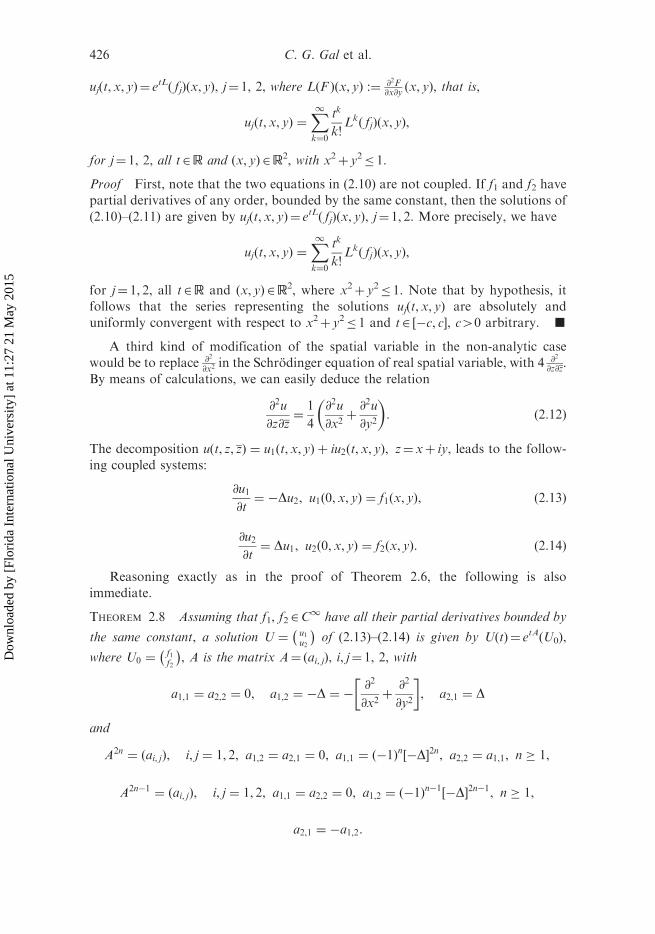
A third kind of modification of the spatial variable in the non-analytic case

would be to replace @2

@x2in the Schrodinger equation of real spatial variable, with 4 @2

@z@z.

By means of calculations, we can easily deduce the relation

@2u

@z@z¼

1

4

@2u

@x2þ@2u

@y2

� �: ð2:12Þ

The decomposition uðt, z, zÞ ¼ u1ðt,x, yÞ þ iu2ðt, x, yÞ, z¼ xþ iy, leads to the follow-

ing coupled systems:

@u1@t¼ �Du2, u1ð0, x, yÞ ¼ f1ðx, yÞ, ð2:13Þ

@u2@t¼ Du1, u2ð0, x, yÞ ¼ f2ðx, yÞ: ð2:14Þ

Reasoning exactly as in the proof of Theorem 2.6, the following is also

immediate.

THEOREM 2.8 Assuming that f1, f22C1 have all their partial derivatives bounded by

the same constant, a solution U ¼�u1u2

�of (2.13)–(2.14) is given by U(t)¼ etA(U0),

where U0 ¼�f1f2

�, A is the matrix A¼ (ai, j), i, j¼ 1, 2, with

a1,1 ¼ a2,2 ¼ 0, a1,2 ¼ �D ¼ �@2

@x2þ@2

@y2

� �, a2,1 ¼ D

and

A2n ¼ ðai, jÞ, i, j ¼ 1, 2, a1,2 ¼ a2,1 ¼ 0, a1,1 ¼ ð�1Þn½�D�2n, a2,2 ¼ a1,1, n � 1,

A2n�1 ¼ ðai, jÞ, i, j ¼ 1, 2, a1,1 ¼ a2,2 ¼ 0, a1,2 ¼ ð�1Þn�1½�D�2n�1, n � 1,

a2,1 ¼ �a1,2:

426 C. G. Gal et al.

Dow

nloa

ded

by [

Flor

ida

Inte

rnat

iona

l Uni

vers

ity]

at 1

1:27

21

May

201

5

Proof The system (2.13)–(2.14) can be rewritten as

dU

dt¼ AU, Uð0Þ ¼

f1f2

� �:¼ U0:

The solution has the form U(t)¼ etA(U0). Finally, the powers An, n2N, can be

obtained from simple calculations. g

Remark 2.9 The formula U(t)¼ etA(U0), in the statements of Theorem 2.7 (for

L¼DH) and Theorem 2.8 (for L¼�D) can be used to deduce more explicit

representations of the solutions U ¼�u1u2

�. In particular, we have

u1ðt, x, yÞ

u2ðt, x, yÞ

� �¼X1k¼0

tk

k!Ak f1ðx, yÞ

f2ðx, yÞ

� �,

where

Ak f1ðx, yÞ

f2ðx, yÞ

� �¼ð�1Þk=2Lkð f1Þðx, yÞ

ð�1Þk=2Lkð f2Þðx, yÞ

!,

for k-even number and

Ak f1ðx, yÞ

f2ðx, yÞ

� �¼ð�1Þðk�1Þ=2Lkð f2Þðx, yÞ

ð�1Þðk�1Þ=2Lkð f1Þðx, yÞ

!,

for k-odd number. Simple calculations show that

u1ðt, x, yÞ ¼X1

k¼0;k-even

tk

k!ð�1Þk=2Lkð f1Þðx, yÞ þ

X1k¼0;k-odd

tk

k!ð�1Þðk�1Þ=2Lkð f2Þðx, yÞ

and

u2ðt, x, yÞ ¼X1

k¼0;k-even

tk

k!ð�1Þk=2Lkð f2Þðx, yÞ þ

X1k¼0;k-odd

tk

k!ð�1Þðk�1Þ=2Lkð f1Þðx, yÞ:

3. Higher order Schrodinger type equations with complex spatial variables

The representation (2.1) of the solution in Theorem 2.1, (i), suggests attaching to

f2A(DR) and p2N, the more general transformation (well-defined for all jzj5R)

T ½ p�ðtÞð f ÞðzÞ ¼X1k¼0

ake�ikptzk ¼

X1k¼0

ake�ikptrkei’k, z ¼ rei’, r5R, t2R: ð3:1Þ

If p¼ 2, then clearly T [2](t)( f )(z) is the same as the complex convolution integral

given by (2.1). Following a similar strategy that was applied to higher order heat

equations in [3], a simple calculation shows that if p¼ 1, then T [p](t)( f )(z) satisfies

Complex Variables and Elliptic Equations 427

Dow

nloa

ded

by [

Flor

ida

Inte

rnat

iona

l Uni

vers

ity]

at 1

1:27

21

May

201

5

the differential equation

i@T ½ p�ðtÞð f ÞðzÞ

@t�@T ½ p�ðtÞð f ÞðzÞ

@’¼ 0,

while for p� 2, T [p](t)( f )(z) satisfies

i@T ½ p�ðtÞð f ÞðzÞ

@t�@pT ½ p�ðtÞð f ÞðzÞ

@’p¼ 0, if p ¼ 2ð2j Þ, j ¼ 1, 2, . . . ,

and we can ask

i@T ½ p�ðtÞð f ÞðzÞ

@tþ@pT ½ p�ðtÞð f ÞðzÞ

@’p¼ 0, if p ¼ 2ð2jþ 1Þ, j ¼ 0, 1, . . . , :

Denoting p¼ 2q, it follows that u2q(t, z)¼T [2q](t)( f )(z) satisfies

i@u2qðt, zÞ

@tþ ð�1Þqþ1

@2qu2qðt, zÞ

@’2q¼ 0, ðt, zÞ 2 0, þ1ð Þ �DR, z ¼ rei’, z 6¼ 0 ð3:2Þ

subject to the initial condition

u2qð0, zÞ ¼ f ðzÞ, z2DR, f2AðDRÞ: ð3:3Þ

Our goal now is to study (3.2)–(3.3).

Remark 3.1 The initial value problem (3.2)–(3.3) suggests that one may also

consider the Cauchy problem for the following higher order Schrodinger equation

with real spatial variable x, as follows:

i@u2qðt, xÞ

@tþ ð�1Þqþ1

@2qu2qðt, xÞ

@x2q¼ 0, ðt, xÞ 2 0,þ1ð Þ � R, ð3:4Þ

with initial condition

u2qð0, xÞ ¼ f ðxÞ, x2R, ð3:5Þ

where f and u¼ u2q, q� 2, are complex valued. Fourth-order Schrodinger equations

(q¼ 2) have been introduced by Karpman [15] to study the role of fourth-order

dispersion terms in the propagation of intense laser beams in a bulk medium. Sharp

dispersive estimates for the biharmonic (i.e. q¼ 2) Schrodinger operator in (3.4) have

recently been obtained in [16]. The study of (3.4)–(3.5) for arbitrary q� 2 remains an

open question.

In the remaining part of this article, we will only deal with (3.2)–(3.3). Following

our work in [3], and arguing as in the proof of Theorem 2.1, the main result of this

section is as follows.

428 C. G. Gal et al.

Dow

nloa

ded

by [

Flor

ida

Inte

rnat

iona

l Uni

vers

ity]

at 1

1:27

21

May

201

5

THEOREM 3.2 Let q2N, q� 2, R41 and f2A(DR). Let u2q(t, z)¼T [2q](t)( f )(z) begiven by (3.1).

(I) For all z2Dr with 1� r5R and t2R, the following estimate holds:

ju2qðt, zÞ � f ðzÞj �t2

2

X1k¼0

jakjk4qrk þ jtj

X1k¼0

jakjk2qrk,

whereP1

k¼0 jakjk4qrk 51, from f (4q)2A(DR).

(II) For all z2Dr with 1� r5R and t, s2R, we have:

ju2qðt, zÞ � u2qðs, zÞj � 2X1k¼0

jakjk2qrkjt� sj:

(III) (T [2q](t), t2R) is a (C0)-group of linear operators, locally equicontinuous onthe locally convex space A(DR) and the unique solution (that belongs toA(DR), for each fixed t) of the Cauchy problem (3.2)–(3.3).

Proof (I) Let jzj � r. We have

ju2qðt, zÞ � f ðzÞj ¼X1k¼0

akzk½e�ik

2qt � 1�

����������

¼X1k¼0

akzk½�2 sin2ðk2qt=2Þ þ i sinðk2qt=2Þ � cosðk2qt=2Þ�

����������

�X1k¼0

jakjrkj2 sin2ðk2qt=2Þj þ

X1k¼0

jakjrkj2 sinðk2qt=2Þj

�t2

2

X1k¼0

jakjk4qrk þ jtj

X1k¼0

jakjk2qrk,

where we have used the well-known inequality jsin(x)j � jxj for all x2R.(II) We have

ju2qðt, zÞ � u2qðt, sÞj ¼X1k¼0

akzk½e�ik

2qt � e�ik2qs�

����������

¼X1k¼0

½cosðk2qtÞ � cosðk2qsÞ � iðsinðk2qtÞ � sinðk2qsÞÞ�

����������

¼X1k¼0

akzk �2 sin

k2qðtþ sÞ

2

� �sin

k2qðt� sÞ

2

� ��������2i sin

k2qðt� sÞ

2

� �cos

k2qðtþ sÞ

2

� ������� 4

X1k¼0

jakjrk sin

k2qðt� sÞ

2

� ��������� � 2

X1k¼0

jakjk2qrkjt� sj:

(III) It is immediate that T [2q](tþ s)¼T [2q](t)(T [2q](s)), for all t, s2R. From (ii),we have T [2q](0)¼ I; the strong continuity of T [2q](�) follows from (iii). Therefore,according to, e.g. [7, p. 232], (T [2q](t))t2R is a C0-group of linear operators. Moreover,

Complex Variables and Elliptic Equations 429

Dow

nloa

ded

by [

Flor

ida

Inte

rnat

iona

l Uni

vers

ity]

at 1

1:27

21

May

201

5

since A(DR) is a Frechet space, (T [2q](t))t2R is locally equicontinuous on A(DR) [8,9].

Finally, reasoning exactly as in the proof of Theorem 2.1, (iv), it follows that

u(t, z)¼T [2q](t)( f )(z) is the unique solution of (3.2)–(3.3). g

References

[1] L.C. Evans, Partial Differential Equations, Graduate Studies in Mathematics, Vol. 19,

American Mathematical Society, Providence, RI, 1998.

[2] C.G. Gal, S.G. Gal, and J.A. Goldstein, Evolution equations with real-time variable and

complex spatial variables, Complex Var. Elliptic Eqns 53(8) (2008), pp. 753–774.

[3] C.G. Gal, S.G. Gal, and J.A. Goldstein, Higher order heat and Laplace type equations with

real-time variable and complex spatial variable, Complex Var. Elliptic Eqns 55(4) (2010),

pp. 357–373.[4] C.G. Gal, S.G. Gal, and J.A. Goldstein, Wave and telegraph equations with real-time

variable and complex spatial variables, Complex Var. Elliptic Eqns (accepted).[5] C.G. Gal, S.G. Gal, and J.A. Goldstein, Burgers and Black-Merton-Scholes equations

with real-time variable and complex spatial variable (submitted).[6] M. Abramowitz and I.A. Stegun, Handbook of Mathematical Functions with Formulas,

Graphs, and Mathematical Tables, Dover, New York, 1965.[7] K. Yosida, Functional Analysis, Springer-Verlag, Berlin, 1980.

[8] T. Komura, Semi-groups of operators in locally convex spaces, J. Funct. Anal. 2 (1968),

pp. 258–296.

[9] F. Terkelsen, On semigroups of operators in locally convex spaces, Proc. Am. Math. Soc.

22 (1969), pp. 340–343.

[10] J.A. Goldstein, Semigroups of Linear Operators and Applications, Oxford University

Press, Oxford, 1985.

[11] P.T. Mocanu, T. Bulboaca, and Gr.St. Salagean, Geometric Theory of Univalent

Functions, Casa Cartii de Stiinta, Cluj, 1999 (Romanian).

[12] J.W Alexander, Functions which map the interior of the unit circle upon simple regions,

Ann. Math. 17(1) (1915), pp. 12–22.

[13] P.L. Duren, Univalent Functions, Springer-Verlag, New York, 1983.[14] S. Gaina, E. Campu, and Gh. Bucur, Problem Book in Differential and Integral Calculus,

Vol. II, Editura Tehnnica, Bucharest, 1966 (in Romanian).[15] V.I. Karpman, Stabilization of soliton instabilities by higher-order dispersion: fourth order

nonlinear Schrodinger-type equations, Phys. Rev. E 53(2) (1996), pp. 1336–1339.[16] M. Ben-Artzi, H. Koch, and J.C. Saut, Dispersion estimates for fourth order Schrodinger

equations, C.R.A.S., Ser. 1 330 (2000), pp. 87–92.[17] J.W. Dettman, Applied Complex Variables, Dover, New York, 1965.

430 C. G. Gal et al.

Dow

nloa

ded

by [

Flor

ida

Inte

rnat

iona

l Uni

vers

ity]

at 1

1:27

21

May

201

5