Analytical solutions of nonlinear Schrödinger equation with distributed coefficients

Author's personal copy

Analytical solutions of nonlinear Schrödinger equationwith distributed coefficients

E. Kengne ⇑Département d’informatique et d’ingénierie, Université du Québec en Outaouais, 101 St-Jean-Bosco, Succursale Hull, Gatineau, QC J8Y 3G5, Canada

a r t i c l e i n f o

Article history:Received 17 August 2013Accepted 22 February 2014Available online 24 March 2014

a b s t r a c t

We combine the F-expansion method with the homogeneous balance principle to build astrategy to find analytical solitonic and periodic wave solutions to a generalized nonlinearSchrödinger equation with distributed coefficients, linear gain/loss, and nonlinear gain/absorption. In the case of a dimensionless effective Gross–Pitaevskii equation whichdescribes the evolution of the wave function of a quasi-one-dimensional cigar-shapedBose–Einstein condensate, the building strategy is applied to generate analytical solutions.

� 2014 Elsevier Ltd. All rights reserved.

1. Introduction

The nonlinear Schrödinger (NLS) equation, a basic equa-tion in nonlinear science, is the subject of much currentinterest due to its many applications in natural sciencesuch as biology [1], chemistry [2], communication andalmost all branches of physics and applied mathematicssuch as plasma physics [3], fluid dynamics [4], and nonlin-ear optics as well as condensed matter physics [5]. Becauseof its relevance to fundamental aspects of physics, manymethods for solving standard NLS equation have beenelaborated: Darboux–Bäcklung transform [6], inversescattering transform [7], variational parameter approach[8], and variational method [9].

In this communication, combining several existingmethods for solving the standard NLS equation, we presenta large family of exact nonlinear wave solutions of thegeneralized NLS equation with varying dispersion, nonlin-earity, gain or loss, nonlinear gain or absorption, and exter-nal potential [10–12]. We are mainly interested in thepropagation of solitary waves and waves propagating withperiodic amplitude in the system described by thegeneralized NLS equation under consideration. In general,

soliton propagation in nonlinear systems is governed bythe generalized NLS equation with distributed coefficients

i@w@t¼ PðtÞ

2@2w@x2 þ gðtÞ wj j2w

þ kðtÞx2 þ kðtÞx� �

wþ iecðtÞwþ ivðtÞ wj j2w; ð1Þ

where wðx; tÞ is the complex envelope of the electrical fieldin a co-moving frame, ecðtÞ is the gain/loss function, vðtÞaccounts for the nonlinear gain or absorption, PðtÞ repre-sents the group velocity dispersion, gðtÞ is the functionalnonlinearity parameter, and kðtÞx2 þ kðtÞx represents theexternal potential. We assume that at least one of gðtÞ andvðtÞ is not a null function. In the absence of external poten-tial, Eq. (1) describes the amplification or absorption ofpulses propagating in a single mode optical fiber with dis-tributed dispersion and nonlinearity. In the theory ofBose–Einstein condensates (BECs), Eq. (1) is the quasi-one-dimensional Gross–Pitaevskii (GP) equation [13] andis known as the model equation for the cigar-shaped BEC.In the case of BECs, PðtÞ is the time-modulated dispersion;the functional nonlinearity parameter gðtÞ is the time-vary-ing scattering length, which is negative (positive) for repul-sive (attractive) interatomic interaction; kðtÞ, the strengthof the magnetic trap, may be positive (confining potential)or negative (repulsive potential); the linear term kðtÞx ofthe potential may correspond to the gravitational field or

http://dx.doi.org/10.1016/j.chaos.2014.02.0070960-0779/� 2014 Elsevier Ltd. All rights reserved.

⇑ Tel.: +1 819 643 0402.E-mail addresses: [email protected], [email protected]

Chaos, Solitons & Fractals 61 (2014) 56–68

Contents lists available at ScienceDirect

Chaos, Solitons & FractalsNonlinear Science, and Nonequilibrium and Complex Phenomena

journal homepage: www.elsevier .com/locate /chaos


some linear potentials. It is worth noting that the conden-sate can interact with the normal atomic cloud throughthree-body interaction, which can be phenomenologicallyincorporated by a gain or loss term ecðtÞ, which is a smallparameter related to the feeding (if positive) or loss (if neg-ative) of atoms in the condensate [14–16]. The imaginarypart of the two-body scattering length, vðtÞ wj j2w, accountsfor the two-body loss (here, vðtÞ is related to a dipolar relax-ation). Eq. (1) in the case of the GP equation with distributedcoefficients can be used to describe the control and manage-ment of BEC by properly choosing different time-dependentparameters [17–20]. In the case when kðtÞ ¼ ecðtÞ � 0,Eq. (1) serves as a model to describe the dynamics of thecondensate surface [21]. In this case, k is a constant forcearising from linearizing the harmonic potential near thesurface: k ¼ mx2R;x being the characteristic frequency ofa spherically symmetric harmonic trapping potential, R isthe radius of the condensate, and m is the mass of an atom.Then x is the coordinate normal to the surface such that thebulk of the condensate exists in the region x < 0. In the ab-sence of the loss/gain term ecðtÞ, the potential in Eq. (1) hasrecently been used to study the internal Josephson-liketunneling in two-component BECs [22].

In the next section, we elaborate strategies for findingexact nonlinear wave solutions of Eq. (1). These strategiesare applied in Section 3 in the case of a dimensionlesseffective GP equation, which describes the evolution ofthe wave function of a quasi-one-dimensional cigar-shaped BEC. The main results are summarized in Section 4.

2. Strategies for finding exact analytical solitonic andperiodic solutions

In order to discuss the cases of a variety of achievableprofiles of the generalized NLS equation with time-depen-dent external potential and nonconservative parts and toobtain the corresponding analytical solutions, we assumethe following ansatz:

wðx; tÞ ¼ 1ffiffiffiffiffiffiffiffi‘ðtÞ

p /ðX; TÞ exp gðtÞ þ iUðx; tÞ½ �; ð2aÞ

Uðx; tÞ ¼ aðtÞ þ bðtÞxþ cðtÞx2; ð2bÞ

where X ¼ x=‘ðtÞ;gðtÞ ¼R t

0ecðsÞdsþ gð0Þ, and ‘ðtÞ; TðtÞ;

aðtÞ; bðtÞ, and cðtÞ are real functions of time t satisfyingthe system of ordinary differential equations (ODEs)

dcdt¼2Pc2�k

d‘dt¼�2P‘c

dTdt¼ 1‘2 ;

dbdt¼2Pcb�k

dadt¼ P

2b2:

ð3Þ

Therefore, /ðX; TÞ is defined as a solution of the NLSequation

i@/@T¼ PðtÞ

2@2/

@X2 þ g0ðtÞ /j j2/þ ik0ðtÞ

@/@Xþ iv0ðtÞ /j j

2/; ð4Þ

where g0ðtÞ ¼ ‘ðtÞgðtÞ exp 2gðtÞ½ �; k0ðtÞ ¼ PðtÞ‘ðtÞbðtÞ, andv0ðtÞ ¼ ‘ðtÞvðtÞ exp 2gðtÞ½ �. It is easily seen that in all thedifferential equations of system (3), the functional param-eter cðtÞ appears either explicitly or implicitly. Moreover,the differential equation for cðtÞ involves two physical

coefficients of Eq. (1), the group velocity dispersion PðtÞand the strength of the magnetic trap kðtÞ. In order to solvethe other equations of system (3), one must solve the equa-tion for cðtÞ first. This testifies to the importance of thefunctional parameter cðtÞ. In the mathematical literature,the differential equation for cðtÞ is known as Riccati equa-tion and does not admit analytical solutions for arbitraryPðtÞ and kðtÞ. In order to find analytical solutions of theabove Riccati equation, it is reasonable to make someappropriate transformation: We write this equation as

d2W

dn2 þ2m

�h2 E� VðnÞ½ �W ¼ 0; ð5aÞ

n¼ nðtÞ¼C0

Z t

0PðsÞds; cðtÞ¼� C0

2WdWdn

;2m

�h2 V�Eð Þ¼ 2k

C20P; ð5bÞ

where C0 – 0 is an arbitrary real constant. If the strengthkðtÞ of the magnetic trap is proportional to the time-mod-ulated dispersion PðtÞ, then Eq. (5a) will be a second orderlinear differential equation with constant coefficients andits general solution is easily found. In the case where 2k

C20P

is not a constant, Eq. (5a) coincides with the well-knownSchrödinger equation of quantum mechanics for the wavefunction W ¼ WðnÞ of a particle of mass m moving with an

energy eigenvalue E in a potential VðnÞ ¼ C20mEP þ �h2k

� �=

mC20P

� �. Thus, if the wave function W ¼ WnðnÞ and the

corresponding energy eigenvalue En are known for a givenpotential VðnÞ (here n stands for some set of quantumnumbers), then for any strength kðtÞ of the magnetic trapand any time-modulated dispersion PðtÞ satisfying condi-tion � k

C20P¼ m

�h2 En � Vð Þ, the function

cnðtÞ ¼ �C0

2Wn

dWn

dn

��nðtÞ¼C0

R t

0PðsÞdsþC01

will be a solution of the Riccati equation dcdt ¼ 2Pc2 � k. With

the help of the particular solution cnðtÞ, one may reduce theRiccati equation for cðtÞ to the Bernoulli equation whosegeneral solution can be easily found.

If cðtÞ is a solution of the above Riccati equation, then oneeasily verifies that the other functional parameters ‘ðtÞ, TðtÞ,bðtÞ, and aðtÞ appearing in system (3) are defined as

‘ðtÞ ¼ ‘ð0Þ exp �2R t

0 PðsÞcðsÞds� �

;

TðtÞ ¼ 1‘2ð0Þ

R t0 exp 4

R s0 PðsÞcðsÞds

� dsþ Tð0Þ;

bðtÞ ¼ bð0Þ exp 2R t


�R t

0 kðsÞ exp

2R ts PðsÞcðsÞds

� �ds;

aðtÞ ¼ 12

R t0 PðsÞb2ðsÞdsþ að0Þ;

8>>>>>>>>>><>>>>>>>>>>:ð6Þ

where ‘ð0Þ; Tð0Þ; bð0Þ, and að0Þ are the values at timet ¼ 0 of ‘ðtÞ; TðtÞ; bðtÞ, and aðtÞ, respectively. With thehelp of Eq. (6), we can express the coefficients of the NLSEq. (4) in terms of the coefficients of Eq. (1):

g0ðtÞ ¼ ‘ð0ÞgðtÞexp 2R t

0ecðsÞ�PðsÞcðsÞ� �

dsþ2gð0Þ� �

;

k0ðtÞ ¼ ‘ð0ÞPðtÞ bð0Þ�R t

0 kðsÞexp �2R s

0 PðsÞcðsÞds�

dsh i

;

v0ðtÞ¼ ‘ð0ÞvðtÞexp 2R t

0ecðsÞ�PðsÞcðsÞ� �

dsþ2gð0Þ� �

:

8>>>><>>>>: ð7Þ

E. Kengne / Chaos, Solitons & Fractals 61 (2014) 56–68 57


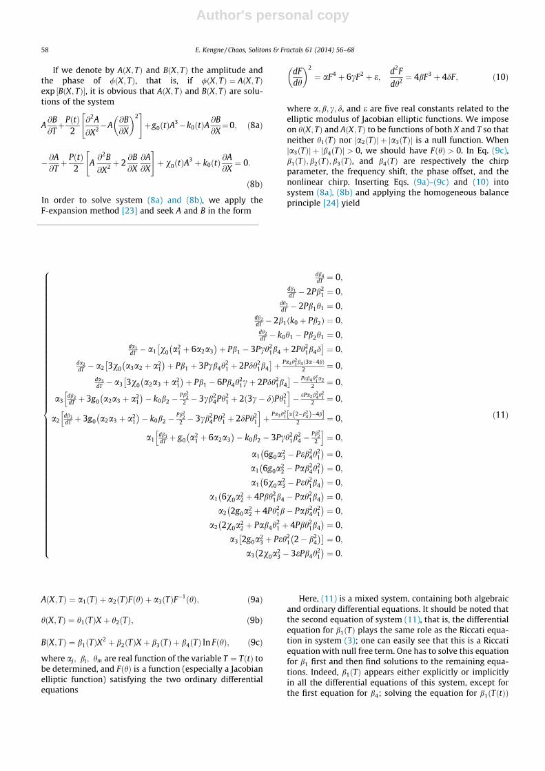
If we denote by AðX; TÞ and BðX; TÞ the amplitude andthe phase of /ðX; TÞ, that is, if /ðX; TÞ ¼ AðX; TÞexp BðX; TÞ½ �, it is obvious that AðX; TÞ and BðX; TÞ are solu-tions of the system

A@B@TþPðtÞ

2@2A

@X2�A@B@X

�2" #

þg0ðtÞA3�k0ðtÞA

@B@X¼0; ð8aÞ

� @A@Tþ PðtÞ

2A@2B

@X2 þ 2@B@X

@A@X

" #þ v0ðtÞA

3 þ k0ðtÞ@A@X¼ 0:

ð8bÞ

In order to solve system (8a) and (8b), we apply theF-expansion method [23] and seek A and B in the form

AðX; TÞ ¼ a1ðTÞ þ a2ðTÞFðhÞ þ a3ðTÞF�1ðhÞ; ð9aÞ

hðX; TÞ ¼ h1ðTÞX þ h2ðTÞ; ð9bÞ

BðX; TÞ ¼ b1ðTÞX2 þ b2ðTÞX þ b3ðTÞ þ b4ðTÞ ln FðhÞ; ð9cÞ

where aj; bl; hm are real function of the variable T ¼ TðtÞ tobe determined, and FðhÞ is a function (especially a Jacobianelliptic function) satisfying the two ordinary differentialequations

dFdh

�2

¼ aF4 þ 6cF2 þ e;d2F

dh2 ¼ 4bF3 þ 4dF; ð10Þ

where a; b; c; d, and e are five real constants related to theelliptic modulus of Jacobian elliptic functions. We imposeon hðX; TÞ and AðX; TÞ to be functions of both X and T so thatneither h1ðTÞ nor a2ðTÞj j þ a3ðTÞj j is a null function. Whena3ðTÞj j þ b4ðTÞj j > 0, we should have FðhÞ > 0. In Eq. (9c),b1ðTÞ; b2ðTÞ; b3ðTÞ, and b4ðTÞ are respectively the chirpparameter, the frequency shift, the phase offset, and thenonlinear chirp. Inserting Eqs. (9a)–(9c) and (10) intosystem (8a), (8b) and applying the homogeneous balanceprinciple [24] yield

Here, (11) is a mixed system, containing both algebraicand ordinary differential equations. It should be noted thatthe second equation of system (11), that is, the differentialequation for b1ðTÞ plays the same role as the Riccati equa-tion in system (3); one can easily see that this is a Riccatiequation with null free term. One has to solve this equationfor b1 first and then find solutions to the remaining equa-tions. Indeed, b1ðTÞ appears either explicitly or implicitlyin all the differential equations of this system, except forthe first equation for b4; solving the equation for b1ðTðtÞÞ

db4dT ¼ 0;

db1dT � 2Pb2

1 ¼ 0;dh1dT � 2Pb1h1 ¼ 0;

db2dT � 2b1 k0 þ Pb2ð Þ ¼ 0;

dh2dT � k0h1 � Pb2h1 ¼ 0;

da1dT � a1 v0 a2

1 þ 6a2a3�

þ Pb1 � 3Pch21b4 þ 2Ph2

1b4d� �

¼ 0;da2dT � a2 3v0 a3a2 þ a2

1

� þ Pb1 þ 3Pcb4h

21 þ 2Pdh2

1b4

� �þ Pa3h2

1b4 3a�4bð Þ2 ¼ 0;

da3dT � a3 3v0 a2a3 þ a2

1

� þ Pb1 � 6Pb4h

21cþ 2Pdh2

1b4

� �� Peb4h2

1a2

2 ¼ 0;

a3db3dT þ 3g0 a2a3 þ a2

1

� � k0b2 �

Pb22

2 � 3cb24Ph2

1 þ 2 3c� dð ÞPh21

h i� ePa2b2

4h21

2 ¼ 0;

a2db3dT þ 3g0 a2a3 þ a2

1

� � k0b2 �

Pb22

2 � 3cb24Ph2

1 þ 2dPh21

h iþ Pa3h2

1 a 2�b24ð Þ�4b½ �

2 ¼ 0;

a1db3dT þ g0 a2

1 þ 6a2a3�

� k0b2 � 3Pch21b

24 �

Pb22

2

h i¼ 0;

a1 6g0a23 � Peb2

4h21

� ¼ 0;

a1 6g0a22 � Pab2

4h21

� ¼ 0;

a1 6v0a23 � Peh2

1b4

� ¼ 0;

a1 6v0a22 þ 4Pbh2

1b4 � Pah21b4

� ¼ 0;

a2 2g0a22 þ 4Ph2

1b� Pab24h

21

� ¼ 0;

a2 2v0a22 þ Pab4h

21 þ 4Pbh2

1b4

� ¼ 0;

a3 2g0a23 þ Peh2

1 2� b24

� � �¼ 0;

a3 2v0a23 � 3ePb4h

21

� ¼ 0:

8>>>>>>>>>>>>>>>>>>>>>>>>>>>>>>>>>>>>>>>>>>>>>>>>>>>><>>>>>>>>>>>>>>>>>>>>>>>>>>>>>>>>>>>>>>>>>>>>>>>>>>>>:

ð11Þ

58 E. Kengne / Chaos, Solitons & Fractals 61 (2014) 56–68


yields b1ðtÞ ¼ ‘2ð0Þb1ð0Þ

‘2ð0Þ�2b1ð0ÞR t

0PðsÞ exp 4

R s

0PðsÞcðsÞds

� �ds

, where b1ð0Þ

is the value of b1 at time t ¼ 0. It is obvious that system(11) is incompatible if a1a2a3 – 0. Thus, for its compatibil-ity, we must have a1a2a3 ¼ 0. Because we are interested innon trivial solutions of Eq. (1), at least one of a1ðTÞ;a2ðTÞ,and a3ðTÞ is a non null function of T. One easily verifies thatconditions a2ðTÞ � 0 and a1ðTÞa3ðTÞ– 0 lead togðtÞ ¼ vðtÞ ¼ 0.

(1) Case a1 ¼ a3 ¼ 0. In this case, system (11) becomes

db4dT ¼eb4¼0;

db1dT �2Pb2

1¼0;db2dT �2b1 k0þPb2ð Þ¼0;

dh1dT �2Pb1h1¼0;

dh2dT �k0h1�Pb2h1¼0;

da2dT �a2 Pb1þPb4 3cþ2dð Þh2

1

h i¼0;

db3dT �k0b2�

Pb22

2 þP 2d�3cb24

� �h2

1¼0;

2g0a22þP 4b�ab2

4

� �h2

1¼0;

2v0a22þPb4 aþ4bð Þh2

1¼0:

8>>>>>>>>>>>>>>>>>>>><>>>>>>>>>>>>>>>>>>>>:

ð12Þ

The last two equations in system (12) impose complemen-tary conditions on a; b; g0 and v0. In this system, it is rea-sonable to consider b4 ¼ 0 only in the case when v0 ¼ 0,that is, when the cubic dissipative term is absent fromEq. (1). It is important to notice that in this case, it is alsopossible to work with b4 – 0. Thus, one must impose onthe coefficients a and b in Eq. (10) to satisfy the conditionaþ 4b ¼ 0.

(2) Case a1ðTÞ � a2ðTÞ � 0. In this case, system (11)becomes

db4dT ¼b4 3a�4bð Þ¼0;

db1dT �2Pb2

1¼0;dh1dT �2Pb1h1¼0;

db2dT �2b1 k0þPb2ð Þ¼0;

dh2dT �k0h1�Pb2h1¼0;

da3dT �a3 Pb1þ2Ph2

1b4 d�3cð Þh i

¼0;

db3dT �k0b2�

Pb22

2 þP 6c�2d�3cb24

� �h2

1¼0;

b24aþ4b�2a¼0;

2g0a23þPe 2�b2

4

� �h2

1¼0;

2v0a23�3eb4Ph2

1¼0:

8>>>>>>>>>>>>>>>>>>>>>><>>>>>>>>>>>>>>>>>>>>>>:

ð13Þ

In the presence of the cubic dissipative term in Eq. (1),we obtain, from the last equation of system (13), thateb4 – 0. To satisfy the third last equation, we must havea ¼ b ¼ 0.

(3) Case a1ðTÞ � 0;a2a3 – 0. In this case, system (11)contains two ordinary differential equations for b3.For its compatibility, these two ODEs must coincide.If we impose on a2ðTÞ; a3ðTÞ; b4; a; b; d, and c tosatisfy the relationship

eb24a

22þ4 2d�3cð Þa2a3þ 2a�ab2

4�4b� �

a23¼0; ð14Þ

then the two ODEs will become identical.(4) Case a3ðTÞ � 0; a1a2 – 0. For the compatibility of

system (11) in this last case, we must haveeb4 ¼ Pdh2

1 þ g0a21 � 0.

After the above transformations, the solution wðx; tÞ ofEq. (1) becomes

wðx;tÞ¼

a1ðTÞþa2ðTÞF h1ðTÞ‘ðtÞ xþh2ðTÞh i

þ a3ðTÞ

Fh1 ðTÞ‘ðtÞ xþh2ðTÞh i

ffiffiffiffiffiffiffiffi‘ðtÞ

p�exp gðtÞþ i

‘2ðtÞcðtÞþb1ðTÞ‘2ðtÞ

x2þ‘ðtÞbðtÞþb2ðTÞ‘ðtÞ

("

xþaðtÞþb3ðTÞþb4ðTÞln Fh1ðTÞ‘ðtÞ xþh2ðTÞ

� �� : ð15Þ

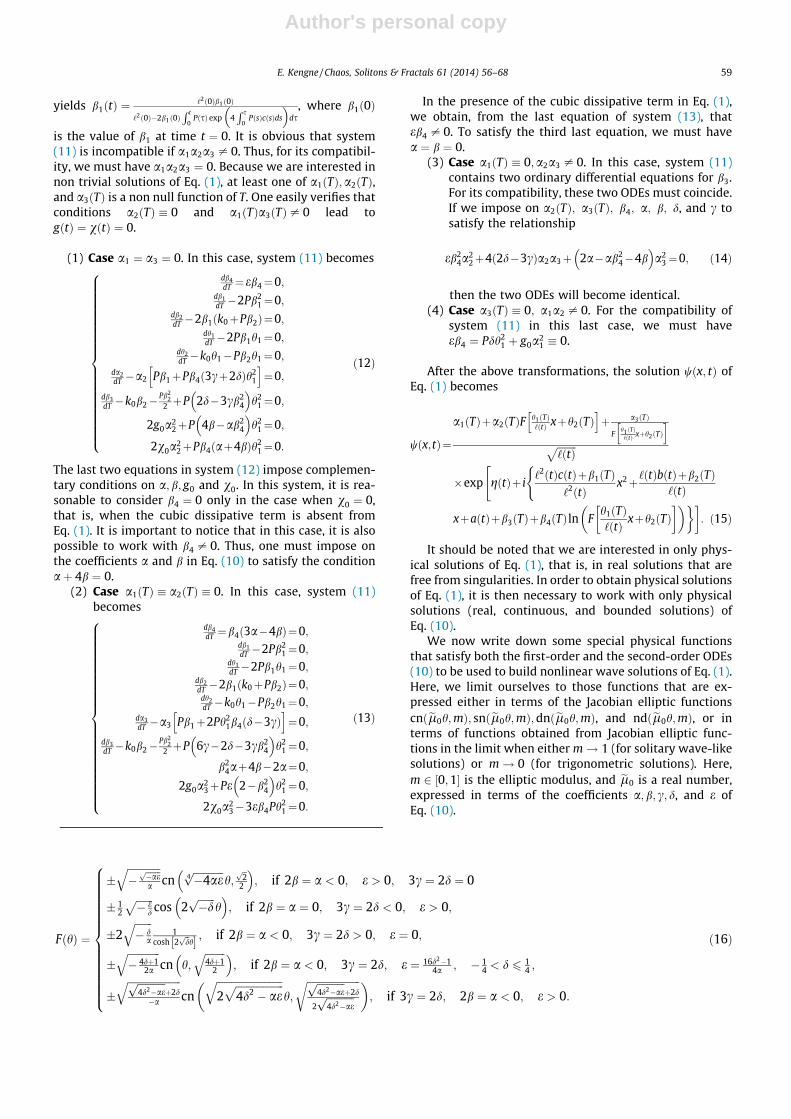
It should be noted that we are interested in only phys-ical solutions of Eq. (1), that is, in real solutions that arefree from singularities. In order to obtain physical solutionsof Eq. (1), it is then necessary to work with only physicalsolutions (real, continuous, and bounded solutions) ofEq. (10).

We now write down some special physical functionsthat satisfy both the first-order and the second-order ODEs(10) to be used to build nonlinear wave solutions of Eq. (1).Here, we limit ourselves to those functions that are ex-pressed either in terms of the Jacobian elliptic functionscnðel0h;mÞ; snðel0h;mÞ;dnðel0h;mÞ, and ndðel0h;mÞ, or interms of functions obtained from Jacobian elliptic func-tions in the limit when either m! 1 (for solitary wave-likesolutions) or m! 0 (for trigonometric solutions). Here,m 2 ½0;1� is the elliptic modulus, and el0 is a real number,expressed in terms of the coefficients a; b; c; d, and e ofEq. (10).

FðhÞ ¼

�ffiffiffiffiffiffiffiffiffiffiffiffiffi�ffiffiffiffiffiffi�aep

a

qcn

ffiffiffiffiffiffiffiffiffiffiffiffi�4ae4p

h;ffiffi2p

2

� �; if 2b ¼ a < 0; e > 0; 3c ¼ 2d ¼ 0

� 12

ffiffiffiffiffiffiffi� e

d

pcos 2

ffiffiffiffiffiffiffi�dp

h� �

; if 2b ¼ a ¼ 0; 3c ¼ 2d < 0; e > 0;

�2ffiffiffiffiffiffiffi� d

a

q1

cosh 2ffiffidp

h½ � ; if 2b ¼ a < 0; 3c ¼ 2d > 0; e ¼ 0;

�ffiffiffiffiffiffiffiffiffiffiffiffiffi� 4dþ1

2a

qcn h;

ffiffiffiffiffiffiffiffi4dþ1

2

q� �; if 2b ¼ a < 0; 3c ¼ 2d; e ¼ 16d2�1

4a ; � 14 < d 6 1

4 ;

�ffiffiffiffiffiffiffiffiffiffiffiffiffiffiffiffiffiffiffiffiffiffiffiffiffiffiffiffiffiffiffiffi

4d2�aep

þ2d�a

qcn

ffiffiffiffiffiffiffiffiffiffiffiffiffiffiffiffiffiffiffiffiffiffiffiffiffiffi2

ffiffiffiffiffiffiffiffiffiffiffiffiffiffiffiffiffiffiffi4d2 � ae

pqh;

ffiffiffiffiffiffiffiffiffiffiffiffiffiffiffiffiffiffiffiffiffiffiffiffiffiffiffiffiffiffiffiffi4d2�aep

þ2d

2ffiffiffiffiffiffiffiffiffiffiffi4d2�aep

r �; if 3c ¼ 2d; 2b ¼ a < 0; e > 0:

8>>>>>>>>>>>>>><>>>>>>>>>>>>>>:

ð16Þ



It is important to note that, in the case wherea3ðTÞj j þ b4ðTÞj j > 0, only the two solutions of Eq. (18) will

be used to generate bounded nonlinear wave solutions ofEq. (1). In fact, with the choice of the ‘‘+’’ sign, they definea positive function FðhÞ. We also notice that the hyperbolic

functions FðhÞ ¼ �2ffiffiffiffiffiffiffi� d

a

q1

cosh 2ffiffidp

h½ � and FðhÞ ¼ �ffiffiffiffiffiffiffiffi� 2d

a

qtanhffiffiffiffiffiffiffiffiffi

�2dp

h� �

obtained from Eqs. (16) and (17) will be associ-

ated with the bright and dark solitary wave-like solutionsof Eq. (1), respectively.

Let us take a look at the special case when h1ðTÞ ¼ h10 isa constant. It follows from system (11) thathðX; TÞ ¼ h10 X þ h2ðTÞ=h10½ �. If, for simplicity, we limitourselves to the case when a1ðTÞ ¼ b4ðTÞ ¼ 0 and a2ðTÞand a3ðTÞ are constants, the corresponding FðhÞ leads tothe following traveling wave solution of Eq. (4):

/ðX; TÞ ¼ a20F h10 X þ h2ðTÞ=h10½ �½ � þ a30

F h10 X þ h2ðTÞ=h10½ �½ �

� exp i b1ðTÞX2 þ b2ðTÞX þ b3ðTÞ

n oh i:

In this special case, each of the above Jacobian ellipticfunctions leads to a solution of Eq. (4) of the following form

/ðX;TÞ ¼ K10qn lðXþh2ðTÞ=h10Þ;mð Þþ K20

qn lðXþh2ðTÞ=h10Þ;mð Þ

� exp i b1ðTÞX2þb2ðTÞXþb3ðTÞ

n oh i; ð19Þ

where qn is any of the Jacobian elliptic functions cn , sn;dnand nd appearing in Eqs. (16)–(18). In Eq. (19), K20 appearsonly for functions from (18). When K20 ¼ 0 (i.e., a30 ¼ 0)and h2ðTÞ=h10 ¼ tT, Eq. (19) gives the so-called start super-position solution [25] which leads to the following possiblesuperposition solution [26] of Eq. (4)

e/ðX; TÞ ¼Xqk¼1

K10qn lðX þ tpTÞ þ nðk� 1ÞKðmÞq

;m �

exp i b1ðTÞX2 þ b2ðTÞX þ b3ðTÞn oh i

; ð20Þ

where n 2 f2;4g and KðmÞ denotes the complete ellipticintegral of first kind. The number q is an integer, and thespeed tp is to be determined by using certain remarkableproperties of Jacobian elliptic functions. Under the condi-tions of the existence of the possible superposition solution(20), system (11) becomes

b1 ¼ b4 ¼ 0; b2 ¼ b20; a2 ¼ a20; a220g0 þ 2bh2

10

P ¼ 0; v0 ¼ 0; k0 þ b20P ¼ const: ¼ t0;

h2ðTÞ ¼ h10 k0 þ b20Pð ÞT; db3

dT� k0b20 þ 2Pdh2

10 �Pb2

20

2¼ 0:

ð21Þ

As an example, we build a superposition solution withan arbitrary q and n ¼ 2 for the dn solution of Eq. (18):

e/ðX; TÞ ¼ KðX; TÞXqj¼1

dn lðX þ tqTÞ þ 2ðj� 1ÞKðmÞq

;m �

;

ð22Þ

where KðX; TÞ ¼ K0 exp i b1ðTÞX2 þ b2ðTÞX þ b3ðTÞn oh i

; l ¼

h10

ffiffiffiffiffiffi3aca�b

q;K0 ¼ �

ffiffiffiffiffiffi3c

b�a

q, and m ¼

ffiffiffiffi2ba

q. Inserting e/ðX; TÞ

(denoting qnj ¼ qn lðX þ tqTÞ þ 2q�1ðj� 1ÞKðmÞ;m� �

) intoEq. (18) and separating the real and imaginary parts, weobtain

db3

dT� P

2b2

20 � k0b20

� Xqj¼1

dnj �P2l2m2

Xqj¼1

dnjcn2j � sn2

j dnj

� �

þ g0K20

Xqj¼1

dnj

!3

¼ 0; ð23aÞ

ilm2 tq � k0 � b20P� �Xq

j¼1

snjcnj ¼ 0: ð23bÞ

For q ¼ 2, we use the Jacobian elliptic functions’ iden-tity dn1dn2 ¼

ffiffiffiffiffiffiffiffiffiffiffiffiffi1�mp

[27] and simplify Eq. (23a) asfollows:

db3

dT� k0b20 �

P2

b220 þ 3g0K

20

ffiffiffiffiffiffiffiffiffiffiffiffiffi1�mp

þP 2�m2�

l2

2

�

�X2

j¼1

dnj þ g0K20 � Pl2

� �X2

j¼1

dn3j ¼ 0:

After replacing l;m, and K0 by their expressions andusing Eqs. (18) and (21), we obtain

a220ða� 2bÞðb� aÞ � 6ba

ffiffiffiffiffiffiffiffiffiffiffiffiffiffiffiffiffiffiffi1�

ffiffiffiffiffiffi2ba

rs0@ 1AX2

j¼1

dnj

� a 2b� aa220

� X2

j¼1

dn3j ¼ 0:

FðhÞ¼

�12

ffiffiffiffiffiffi� e

d

psin 2

ffiffiffiffiffiffiffi�dp

h� �

; if 2b¼a¼0; 3c¼2d<0; e>0;

�ffiffiffiffiffiffiffiffi�2d

a

qtanh

ffiffiffiffiffiffiffiffiffi�2dp

h� �

; if 2b¼a>0; 3c¼2d<0; ea�4d2 ¼0;

�ffiffiffiffiffiffiffiffiffiffiffiffiffiffiffiffiffiffiffiffiffi

�effiffiffiffiffiffiffiffiffiffiffi4d2�eap

þ2d

qsn

ffiffiffiffiffiffiffiffiffiffiffiffiffiffiffiffiffiffiffiffiffiffiffiffiffiffiffiffiffiffiffiffiffiffiffiffiffi�2d�

ffiffiffiffiffiffiffiffiffiffiffiffiffiffiffiffiffiffi4d2�ea

pqh;�2dþ

ffiffiffiffiffiffiffiffiffiffiffi4d2�eapffiffiffiffi

eap

�; if 2b¼a>0; 3c¼2d; e>0; d<�

ffiffiffiffieap

2 :

8>>>>><>>>>>:ð17Þ

FðhÞ ¼�

ffiffiffiffiffiffi3c

b�a

qdn

ffiffiffiffiffiffi3aca�b

qh;

ffiffiffiffi2ba

q �; if a < 2b < 0; c b� að Þ > 0; d ¼ 3bc

a ; e ¼ 9c2 a�2bð Þa�bð Þ2

;

�ffiffiffiffiffiffiffiffiffiffiffiffiffiffiffiffiffiffiffiffiffiffiffiffiffiffi� 2d�

ffiffiffiffiffiffiffiffiffiffiffi4d2�aep

a

qnd

ffiffiffiffiffiffiffiffiffiffiffiffiffiffiffiffiffiffiffiffiffiffiffiffiffiffiffiffiffiffiffiffiffiffiffiffiffiffiffiffiffiffiffiffiffiffiffiffiffiffiffiffiffiffi4d2 � ae

pþ 2d

qh;

ffiffiffiffiffiffiffiffiffiffiffiffiffiffiffiffiffiffiffiffiffi2ffiffiffiffiffiffiffiffiffiffiffi4d2�aepffiffiffiffiffiffiffiffiffiffiffi4d2�aep

þ2d

r �; if 2b ¼ a < 0; e < 0; 3c ¼ 2d >

ffiffiffiffiffiffiaep

:

8>>><>>>: ð18Þ



This last equality holds if and only if a220 ¼ 2b

a and

ð2b� aÞðb� aÞ þ 3a2

ffiffiffiffiffiffiffiffiffiffiffiffiffiffiffiffiffi1�

ffiffiffiffi2ba

qr¼ 0. Going back to Eq.

(23b) and using Eq. (21), we find tq ¼ const: ¼ t0. Thus,under conditions (21), if we take a2

20 ¼ 2b=a with a and b

satisfying condition ð2b� aÞðb� aÞ þ 3a2

ffiffiffiffiffiffiffiffiffiffiffiffiffiffiffiffiffi1�

ffiffiffiffi2ba

qr¼ 0,

then

e/ðX;TÞ¼KðX;TÞX2

j¼1

dn lðXþt0TÞþðj�1ÞKðmÞ;mð Þ ð24Þ

will be a superposition solution of Eq. (4).As one can easily see from Eq. (23b), the speed for any

existing superposition solution is tq ¼ const: ¼ t0.By combining an F-expansion method with the

homogeneous balance principle, we have thus presenteda strategy of finding analytical solutions of a class of com-plex cubic nonlinear Schrödinger equation with distributedcoefficients. This combination appears as an explicit vari-ant of the inverse-problem method of finding analyticalsolutions of partial differential equations. In the generalform, such a combination has been proposed for the gener-ation of wide classes of exact solutions to the stationaryGross–Pitaevskii equation [28].

3. Applications to a dimensionless effective GP equationfor wave functions of a quasi-one-dimensional cigar-shaped BEC

In this section, we apply the results of the previous sec-tion to generate analytical solutions of a dimensionlesseffective GP equation that describes the evolution of thewave function of a quasi-one-dimensional cigar-shapedBEC.

For simplicity, the above solution strategies, in the caseof a dimensionless effective GP equation, are applied whenthe strength kðtÞ of the magnetic trap is proportional to thetime-modulated dispersion PðtÞ. Let �ek2

0=2 be the coeffi-cient of proportionality so that kðtÞ ¼ �ek2

0PðtÞ=2. Then,Eqs. (5a) and (5b) become

cðtÞ ¼ek0

2tan ek0

Z t

0PðsÞdsþ arctan

2cð0Þek0

" #; ð25aÞ

cðtÞ ¼ek0

2tanh arctanh

2cð0Þek0

!� ek0

Z t

0PðsÞds

" #; ð25bÞ

where (25a) and (25b) are associated with �ek20=2 and

þek20=2, respectively. The term cðtÞ of form (25a) imposes

a time-periodic driving term in Eq. (4) with frequencyx�, which is nothing but the oscillation frequency. In thisviewpoint, the phase divergence at tn that satisfies the con-

ditionR tn

0 PðsÞds ¼ ð1þ2nÞp

2ek0

� 1ek0

arctan 2cð0Þek0

(with n ¼ 0;�1;

�2, . . .) is understandable. To avoid the singularity, wework with t 2 ½0; t0½\½0;D01½ for some real constant D01 thatshould be taken in such a way that TðtÞ varies from 0 toþ1.

By using ansatz (2a) and the polar form/ðX; TÞ ¼ AðX; TÞ exp iBðX; TÞ½ � of /ðX; TÞ where AðX; TÞ and

BðX; TÞ are defined by system (9a)–(9c), we can write downthe density of condensates in the GP equation when eachof the time-modulated dispersion PðtÞ, time-varying scat-tering length gðtÞ, and time-varying strength of the mag-netic trap kðtÞ are of the special form:

wðx; tÞj j2 ¼ exp 2gðtÞ½ �‘ðtÞ a1ðTÞ þ a2ðTÞFðhÞ þ

a3ðTÞFðhÞ

�� 2; ð26Þ

where ‘ðtÞ and TðtÞ are given by (6), gðtÞ ¼R t

0ecðsÞdsþ

gð0Þ; FðhÞ is any ‘‘physical function’’ satisfying the twoODEs (10), h ¼ hðX; TÞ is defined by Eq. (9b) with

Xðx; tÞ ¼ x‘�1ð0Þ exp 2R t


, and a1ðTÞ;a2ðTÞ;a3ðTÞ; h1ðTÞ, and h2ðTÞ are solutions of system (11). For sim-plicity, we shall use TðtÞ with Tð0Þ ¼ 0. In Eq. (26), we usea3 – 0 only when FðhÞ – 0 for every t 2 ½0; t0½\½0;D01½. Inthe case FðhÞ ¼ 0 for some t� 2 ½0; t0½\½0;D01½, we takea3ðTÞ � 0.

For applying the results of the previous section to adimensionless effective GP equation with special forms ofthe dispersion PðtÞ, scattering length gðtÞ, and strength ofthe magnetic trap kðtÞ, we focus ourselves on the solitarywave-like solutions and solutions of Eq. (1 ) that areexpressed in terms of the Jacobian elliptic function dn.

3.1. Bright and dark solitary wave-like solutions

In this subsection, we use Eqs. (16) and (17) to generatethe bright and dark solitary wave-like solutions of Eq. (1):

jwðx; tÞj2 ¼ exp 2gðtÞ½ �‘ðtÞ

��a1ðTÞ þK01a2ðTÞ

cosh 2ffiffiffidp

hh i

þ a3ðTÞK01

cosh 2ffiffiffidp

hh i��2; ð27Þ

and

jwðx; tÞj2 ¼ exp 2gðtÞ½ �‘ðtÞ

��a1ðTÞ þK02a2ðTÞ tanhffiffiffiffiffiffiffiffiffi�2dp

h� �

þ a3ðTÞK02 tanh

ffiffiffiffiffiffiffiffiffi�2dp

h� �

��2

; ð28Þ

respectively. Here, K01 ¼ �2ffiffiffiffiffiffiffiffiffiffiffiffi�d=a

pand K02 ¼ �

ffiffiffiffiffiffiffiffiffiffiffiffiffiffiffi�2d=a

p.

For the bright and dark solitary waves (27) and (28), thecoefficients of the two ODEs (10) must satisfy the condi-tions 2b ¼ a < 0;3c ¼ 2d > 0; e ¼ 0, and 2b ¼ a > 0;3c ¼ 2d < 0; ea� 4d2 ¼ 0, respectively. For simplicity, welimit ourselves in this subsection to the construction ofexamples of bright and dark solitary wave solutions witha3ðTÞ � 0. Therefore, a2ðTÞ cannot be a null function. Underthe conditions a3ðTÞ � 0 and a2ðTÞ– 0, one can easily ver-ify that only a1ðTÞ � 0 leads to solitary wave solutionswhen at least one of gðtÞ and vðtÞ is not a null function.

After analyzing system (12), we found that for a1ðTÞ � 0and a3ðTÞ � 0, and gðtÞ– 0, bright solitary waves (27) canexist only when the coefficient of the dipolar relaxationvðtÞ is proportional to the time-varying scattering lengthgðtÞ, with a proportionality coefficient 3b4= 2� b2

4

� . The

dark solitary wave (28) may exist only in the absence of



nonlinear gain or absorption, that is, when the last term ofEq. (1) is absent.

It should be noted that Eqs. (27) and (28) under condi-tions a1ðTÞ � 0 and a3ðTÞ � 0 become

wðx;tÞj j2 ¼K201

exp 2gðtÞ½ �a22½TðtÞ�

‘ðtÞ1

cosh2 2ffiffiffidp

h1½TðtÞ� x‘ðtÞþh2½TðtÞ�

� �h i ;wðx;tÞj j2 ¼K2

02exp 2gðtÞ½ �a2

2½TðtÞ�‘ðtÞ tanh2 ffiffiffiffiffiffiffiffiffi

�2dp

h1½TðtÞ�x‘ðtÞþh2½TðtÞ�

�� :

Therefore, the amplitude of the solitary wave is propor-tional to a2

2 TðtÞ½ � exp 2gðtÞ½ �=‘ðtÞ, while its width is propor-tional to �‘ðtÞ=h1ðTÞ. Moreover the center of the solitarywaves is fðtÞ ¼ �‘ðtÞh2 TðtÞ½ �h�1

1 TðtÞ½ � and satisfies the differ-ential equation

d2f

dt2 þ 2 Ptc � Pkþ Ptb1

‘2

�f� k� ð‘bþ b2Þ

P‘dPdt

�¼ 0:

ð29Þ

If the time-dependent strength kðtÞ of the linear part of

the potential is chosen as kðtÞ ¼ ð‘bþb2ÞP‘

dPdt , then Eq. (29)

means that the center of mass of the macroscopic wavepacket behaves like a classical particle, and allows one tomanipulate the motion of bright solitary waves in BEC sys-tems by controlling the dispersion and external harmonictrapping potential. It is important to note that in the case

when kðtÞ ¼ ð‘bþb2ÞP‘

dPdt ; bðtÞ and b2ðtÞ should satisfy the linear

homogeneous differential system

ddt

bðtÞb2ðtÞ

� ¼

2P2c�PtP � Pt

P‘2b1P‘

2b1P‘2

" #bðtÞb2ðtÞ

� ;

where Pt ¼ dPdt ; b1ðtÞ ¼ b1ð0Þ

1�2b1ð0ÞR t

0PðsÞ‘2 ðsÞ

ds, and cðtÞ is given by

either (25a) or (25b).

3.1.1. Example of bright and dark solitary-wave propagationwith a solution of the Riccati equation chosen from Eq. (25a)

For the first example of bright and dark solitary-wavesolutions with a1ðTÞ � 0 and a3ðTÞ � 0, we follow Yuceet al. [29] and consider the time-varying scattering length

gðtÞ ¼ 4m�1p�h2eg 1þ D= B0 � BðtÞ½ �f g, where 4m�1p�h2eg isthe asymptotic value of the scattering length far from res-

onance, BðtÞ is the time-dependent externally applied mag-netic field, D is the width of resonance, and B0 is theresonant value of the magnetic field. With this form ofscattering length, we work with a dispersion of the form

PðtÞ ¼ eP 1� D= B1t � B0½ �f g, where either t 2 ½0;B0B�11 ½ or

t 2�B0B�11 ;þ1½. This form of time-modulated dispersion is

dictated by the dependence of the scattering length onthe magnetic field near the Feshbach resonance of coldBEC atoms [29]. Here, the magnetic field B1t is assumedto be linearly ramped in time near the resonance field B0.The parameter D stands for the width of the resonance.Such a dependence is found relevant on both theoretical[29] and experimental [30] grounds. The functional param-eter cðtÞ used in this example is given by Eq. (25a):

cðtÞ ¼ ek02 tan ek0

eP t � DB1

ln t � B0=B1j j� �h i

.

3.1.1.1. Bright solitary-wave solutions. By taking vðtÞ ¼ 3b4=

2� b24

� gðtÞ; b1ðTÞ ¼ 0, and by imposing on BðtÞ to be as in

the expression of gðtÞ taken from the condition

gðtÞ¼a b2

4�2�

32d2‘ð0Þb24h

210

PðtÞexp 2R t

0 PðsÞcðsÞ� ecðsÞ� �ds�2gð0Þ

h iR t

0PðsÞ‘2ðsÞdsþa2ð0Þ

h i2 ;

we have solved system (12) for the bright solitary waveand found

h1¼ h10; b2¼ b20; h2ðtÞ¼ h10

Z t

0

PðsÞ ‘ðsÞbðsÞþb20½ �‘2ðsÞ

ds

þh2ð0Þ; a2ðtÞ¼4b4dh210

Z t

0

PðsÞ‘2ðsÞ

dsþa2ð0Þ;

b3ðtÞ¼Z t

0

PðsÞ 2b20‘ðsÞbðsÞþb220þ4d b2

4�1�

h210

� �2‘2ðsÞ

dtþb3ð0Þ;

where b4 –ffiffiffi2p

; h10 and b20 are three arbitrary real con-stants. Here, bðtÞ is a solution to linear ODEdb=dt ¼ 2Pcb� k.

It appears that in the present example for the bright sol-itary wave-like solution, only the linear gain/loss coefficient

Fig. 1. Density wðx; tÞj j2 given by Eq. (27) for the modulation of the gain/loss parameter ecðtÞ ¼ ec0 1� sin x0t½ �with x0 ¼ 1. (a) and (c) correspond to the lossand feeding of atoms in the condensate and are generated with ec0 ¼ �0:02 and ec0 ¼ 0:02, respectively; (b) corresponds to the absence of the loss andfeeding of atoms in the condensate, i.e., to ec0 ¼ 0. The other parameters are given in the text.



ecðtÞ in Eq. (1) is not submitted to any restriction. By usingthe periodic modulation of the gain/loss parameterecðtÞ ¼ ec0 1� sin x0t½ �, we plot in Fig. 1 the density wðx; tÞj j2

given by Eq. (27) for the set of values of parameter ec0

(ec0 ¼ 0:02; 0; 0:02) with x0 ¼ 1, and a1ðTÞ ¼ a3ðTÞ � 0.Plots (a) and (c) respectively correspond to the loss (nega-tive ec0) and feeding (positive ec0) of atoms in the conden-sate, while case (b) corresponds to the absence of loss andfeeding of atoms in the condensate. For the plots of this fig-ure, we used the parameters eP ¼ 1; D ¼ 1; B0 ¼ 1, B1 ¼ 1,ek0 ¼ 0:05; a ¼ �5; d ¼ 1=2; ‘ð0Þ ¼ 0:97; bð0Þ ¼ 0; h10 ¼2; b20 ¼ 1 ; h2ð0Þ ¼ 0; a2ð0Þ ¼ 5; b3ð0Þ ¼ 0; b4 ¼ 1. Thetime interval t 2 ½0;32:74½ which corresponds toT 2 ½0;þ1½ has been used. Fig. 1 shows that (i) the ampli-tude of the bright solitary wave decreases with the lossparameter and increases with the feeding parameter; (ii)in all the three cases (loss/feeding and without loss/feedingof atoms in the condensate), the bright solitary wave has thesame parabolic trajectory, oriented to the þx-axis; (iii) thewidth of the bright solitary wave varies during its propaga-tion: it first increases, reaches a maximal value, and thendecreases.

3.1.1.2. Dark solitary-wave solutions. To obtain an exampleof solution of system (12) for a dark solitary wave, wechoose to solve (21) in which we already have v0 ¼ 0,meaning that vðtÞ ¼ 0. We then obtain, under the condi-tion k0 þ b20P ¼ const: ¼ t0=h10 – 0 and a2

20g0 þ ah210P ¼ 0,

that

b1 ¼ b4 ¼ 0; b2 ¼ b20; a2 ¼ a20; h2ðTÞ ¼ t0T;

b3ðtÞ ¼Z t

0

PðsÞ 2‘ðsÞbðsÞb20 þ b220 � 4dh2

10

� �2‘2ðsÞ

dt þ b3ð0Þ;

where b20; a20, and h10 are three arbitrary real con-stants.The condition k0 þ b20 P ¼ const: ¼ t0 – 0 imposes

the following form to kðtÞ : kðtÞ ¼ P0 ðtÞ ‘ðtÞbðtÞþb20½ �PðtÞ‘ðtÞ .With this

form for kðtÞ; bðtÞ will then be a solution of the linear ODEdbdt ¼

2P2c�PtP b� b20

PtP‘.The condition a2

20g0 þ ah210P ¼ 0 implies

that BðtÞ appearing in gðtÞmust be taken from the condition

a220‘ðtÞgðtÞ exp 2

R t0ecðsÞdsþ 2gð0Þ

h iþ ah2

10P ¼ 0.As in the

case of the previous example for the bright solitary wave,the linear gain/loss coefficient ecðtÞ in Eq.(1) is free fromany restriction.Using the periodic modulation of the gain/loss parameter ecðtÞ ¼ ec0 1� sin x0t½ � with the set of valuesof the parameter ec0 (ec0 ¼ �0:02;0, and 0:02, we depict in

Fig.2 the density wðx; tÞj j2 given by Eq.(28) for the dark sol-itary wave solution with x0 ¼ 1.Plots (a), (b), and (c) corre-sponding to the loss of atoms (with ec0 ¼ �0:02), to no lossnor feeding of atoms (with ec0 ¼ 0), and to the feeding ofatoms in the (with ec0 ¼ 0:02), respectively, in the conden-sate.To generate the different plots of this figure, the follow-

ing parameters have been used: eP ¼ 1; D ¼ 0:7;B0 ¼ 3:4; B1 ¼ 0:1; ek0 ¼ 0:05; a ¼ 5; d ¼ �1=2; ‘ð0Þ ¼ 0:98;bð0Þ ¼ 0; h10 ¼ 2; b20 ¼ 1; h2ð0Þ ¼ 0; a2ð0Þ ¼ 5; b3ð0Þ ¼ 0;b4 ¼ 1; t0 ¼ 0:05. Here, we have chosen t 2 ½0;32:74½which corresponds to T 2 ½0;þ1½. It is seen from the plotsof this figure that for all three cases (loss, feeding, and noloss nor feeding of atoms in the condensate) the dark soli-tary wave propagates with the same behavior: (i) the ampli-tude of the wave decreases with the loss parameter andincreases with the feeding parameter; (ii) the width of thebright solitary wave varies during its propagation: it first in-creases, reaches a maximal value, and then decreases.

3.1.2. Example of bright and dark solitary-wave propagationwith a1ðTÞ � a3ðTÞ � 0. As a second example for generatingbright and dark solitary-wave solutions witha1ðTÞ � a3ðTÞ � 0, we consider the case when the disper-sion PðtÞ is an exponential function of time, describing a

smooth change from 1 to 1=2; PðtÞ ¼ 12 1þ exp �ed2t

h i� �,

where ed is some arbitrary parameter. The correspondingcðtÞ to be used is given by Eq. (25b) (this means that Pand k are of the same sign). For both the bright and dark

solitary-wave solutions, we use gðtÞ ¼ aP b24�2ð Þh2

1

2‘ðtÞa22

exp �2gðtÞ½ �, where gðtÞ ¼R t

0ecðsÞdsþ gð0Þ. Without loss

of generality, we take b4 ¼ 0.Figs. 3 and 4 present the bright and dark solitary wave

solutions (27) and (28), respectively, witha1ðTÞ � a3ðTÞ � 0 and cð0Þ ¼ ek0=2, and show the effect ofthe chirp function b1ðtÞ on the soliton propagation. For a

Fig. 2. Density wðx; tÞj j2 given by Eq. (28) associated with dark solitary wave with the modulation of the gain/loss parameter ecðtÞ ¼ ec0 1� sinx0t½ � withx0 ¼ 1. (a) and (c) correspond to the loss and feeding of atoms in the condensate and are generated with ec0 ¼ 0:02 and ec0 ¼ 0:02, respectively; (b)corresponds to the absence of the loss and feeding of atoms in the condensate, i.e., to ec0 ¼ 0. The other parameters are given in the text.



better understanding of the importance of the functionalparameter b1ðTÞ, we used different initial conditions b1ð0Þto generate the different plots. In these two figures, plot(a) shows the spatiotemporal evolution of the solitarywave-like solutions, plot (b) shows the curvea2

2ðtÞ‘�1ðtÞe2gðtÞ to which the soliton amplitude is propor-

tional, and plot (c) shows the profile of the solitary wave-likesolution at different times. For each of these two figures, asmall loss ecðtÞ ¼ �0:085 has been added. The coefficient ofthe linear term of the trap potential is taken to be kðtÞ ¼ 1.

The plots of Figs. 3 and 4 are generated forek0 ¼ 0:1; ‘ð0Þ ¼ 1; gð0Þ ¼ �0:1; ed0 ¼ 0:1; bð0Þ ¼ 0:1;h1ð0Þ ¼ 0:1; h2ð0Þ ¼ 0:1; b2ð0Þ ¼ 0:1; b3ð0Þ ¼ 0:1; a2ð0Þ¼ 0:1. Here, as we have mentioned above, we have used dif-ferent initial conditions for b1½TðtÞ� : b1ð0Þ ¼ 0:003 for thetop plots and b1ð0Þ ¼ 0:006 for the bottom plots. In plot(c), panel (I) shows the soliton profile at t0 ¼ 0:1 (red),t0 ¼ 1:5 (green), and t0 ¼ 3 (blue), while panel (II) showsthe soliton profile at t0 ¼ 8 (red), t0 ¼ 9 (green), andt0 ¼ 10 (blue). For Fig. 3 and 4, we used a ¼ �0:1 and

Fig. 4. Effect of the chirp function b1ðtÞ on the motion of the dark solitary wave given by Eq. (28) with a1ðTÞ � a3ðTÞ � 0. (a) Spatiotemporal evolution of thebright solitary wave in the presence of loss of atoms in the condensate with ecðtÞ ¼ �0:085; (b) curve of the coefficient of the amplitude proportionality; (c)soliton profile at different time: panel (I) shows the soliton profile at t0 ¼ 0:1 (red), t0 ¼ 1:5 (green), and t0 ¼ 3 (blue), while panel (II) shows the solitonprofile at t0 ¼ 8 (red), t0 ¼ 9 (green), and t0 ¼ 10 (blue). The top and bottom panels are generated with the initial chirp function b1ð0Þ ¼ 0:003 andb1ð0Þ ¼ 0:006, respectively. To generate these plots, we used a ¼ 0:1 and d ¼ �0:05. The other parameters are given in the text. (For interpretation of thereferences to colour in this figure legend, the reader is referred to the web version of this article.)

Fig. 3. Effect of the chirp function b1ðtÞ on the motion of the bright solitary wave given by Eq. (27) with a1ðTÞ � a3ðTÞ � 0. (a) Spatiotemporal evolution ofthe bright solitary wave in the presence of a loss of atoms in the condensate with ecðtÞ ¼ �0:085; (b) curve of the coefficient of the amplitudeproportionality; (c) soliton profile at different times: panel (I) shows the soliton profile at t0 ¼ 0:1 (red), t0 ¼ 1:5 (green), and t0 ¼ 3 (blue), while panel (II)shows the soliton profile at t0 ¼ 8 (red), t0 ¼ 9 (green), and t0 ¼ 10 (blue). The top and bottom panels are generated with the initial chirp functionb1ð0Þ ¼ 0:003 and b1ð0Þ ¼ 0:006, respectively. To generate these plots, we used a ¼ �0:1 and d ¼ 0:05. The other parameters are given in the text. (Forinterpretation of the references to colour in this figure legend, the reader is referred to the web version of this article.)



d ¼ 0:05, and a ¼ 0:1 and d ¼ �0:05, respectively. The plotsof the top panel show a soliton propagating with a decreas-ing amplitude (this is confirmed by plot (b)) and with a com-pressing width, as it is easily seen from plot (c). From theplots of the bottom panel, we easily see a soliton that firstpropagate with an increasing amplitude, and then with adecreasing amplitude (this is clearly seen from plots (c)).This change in soliton amplitude is confirmed by plot (c)showing the curve of the amplitude proportionality. It is alsoeasily seen from plots (a) and (c) that the soliton propagateswith a compressed width.

3.1.3. Example of bright and dark solitary-wave propagationwith a time-modulated dispersion PðtÞ that is proportional tothe time-varying scattering length gðtÞ. In this example, weshow the effect of the gravitational field and of thefunctional chirp parameter b1ðtÞ on the soliton propaga-tion. We consider the easiest case when a1ðtÞ ¼ a3ðtÞ ¼b4ðtÞ � 0.

It is easy to verify that the system

a1ðtÞ¼a3ðtÞ¼ b4ðtÞ�0;

b1ðtÞ¼ ‘2ð0Þb1ð0Þ


0PðsÞexp 4

R s

0PðsÞcðsÞds

� �ds

h1ðtÞ¼ h1ð0ÞexpR t

02PðsÞb1ðsÞ‘2ðsÞ ds

� �b2ðtÞ¼ b2ð0Þexp

R t0


� �þR t

02k0ðsÞb1ðsÞ

‘2ðsÞ exp 2R ts

PðsÞb1ðsÞ‘2ðsÞ ds

� �ds

h2ðtÞ¼R t

0k0ðsÞþPðsÞb2ðsÞ½ �h1ðsÞ

‘2ðsÞ dsþh2ð0Þ

a2ðtÞ¼a2ð0ÞexpR t


� �;

b3ðtÞ¼R t

02k0ðsÞb2ðsÞþPðsÞ b2

2ðsÞ�4dh21ðsÞ½ �

2‘2ðsÞ dsþb3ð0Þ

8>>>>>>>>>>>>>>>>>>>>>>>>><>>>>>>>>>>>>>>>>>>>>>>>>>:

ð30Þ

defines both bright and dark solitary wave solutions assoon as vðtÞ ¼ 0 and PðtÞ; gðtÞ, and ecðtÞ satisfy therelationship

‘ð0Þa22ð0ÞgðtÞexp 2

Z t

0

ecðsÞ�PðsÞcðsÞ�PðsÞb1ðsÞ‘2ðsÞ

!dsþ2gð0Þ

" #þ2bh2

1ð0ÞPðtÞ¼0: ð31Þ

For this third example, we worked under the conditionthat the time-modulated dispersion PðtÞ was proportionalto the time-varying scattering length gðtÞ with the coeffi-cient of proportionality �‘ð0Þa2

2ð0Þ exp 2gð0Þ½ �=½2bh21ð0Þ�.

According to condition (31), the loss/gain coefficient ecðtÞmust be taken as

ecðtÞ¼ PðtÞcðtÞ

þ 2b1ð0ÞPðtÞ‘2ð0Þexp �4

R t0 PðsÞcðsÞds

� ��2b1ð0Þ

R t0 PðsÞexp 4

R st PðsÞcðsÞds

� ds;

ð32aÞ

PðtÞ ¼ � ‘ð0Þa22ð0Þ exp 2gð0Þ½ �

2bh21ð0Þ

gðtÞ: ð32bÞ

Following Gao et al. [31], in the present example, weconsidered the scattering length gðtÞ [here, we used thesame notation as in [31]]:

g1ðtÞ ¼ �G1q0 cos t

R20

ffiffiffiffiffiffiffiffiffiffiffiffiffiffiffiffiffiffiffiffiffiffiffiffiffiffiffiffiffiffiffiffiffiffiffiffiffiffiffiffiffiffiffiffiffiffiffiffiffiffiffiffiffiffiffiffiffiffiffiffiffiffiffiffiffi1þ tan2

ffiffiffiffiffiffiffiffiffiffiffiffiffiffi2V0q0

pb0 þ sin tð Þ

� �q ;

where b0;V0, and q0 are three real constants to be chosencarefully to avoid the singular points of the tan function.For simplicity, here we consider only the case where thetime-varying strength of the magnetic trap kðtÞ is propor-tional to PðtÞ with coefficient of proportionality ek2

0=2. Forthe solution of the Riccati equation dc=dt ¼ 2Pc2 � k weused expression (25b). Fig. 5 shows the dynamics of thedensity wðx; tÞj j2 corresponding to the bright solitary wave(top panels with b0 ¼ 1=5;V0 ¼ 1=2;q0 ¼ 1=2;R0 ¼ 1, andG1 ¼ 0:05) and the dark solitary wave (bottom panels withb0 ¼ 1;V0 ¼ 1=2;q0 ¼ 1=2;R0 ¼ 1, and G1 ¼ 0:08) given byEqs. (27) and (28), respectively.

The top panels of Fig. 5, which shows the densitywðx; tÞj j2 for the bright solitary wave-solution (27) is gener-

ated with different chirp functional parameter b1ðtÞ, real-ized with the initial values b1ð0Þ ¼ �0:05;0;0:05,corresponding to the labels (a), (b), (c), respectively. Theseplots show that the functional parameter b1ðtÞ has animportant effect on modulating the amplitude of the solu-tion wðx; tÞ. Because of the periodicity of the time-modu-lated dispersion PðtÞ;wðx; tÞ is an explicit breathingsolitary wave solution. The breathing behavior is clearerif we take b1ðtÞ ¼ 0 (see plot (b)), which corresponds, asone may see from Eq. (32a), to the absence of feedingand loss of atoms in the condensate [ecðtÞ � 0]. It is seenfrom the plots of the top panels that the amplitude of thedensity wðx; tÞj j2 is oscillating along the t-axis and showsa strongly breathing behavior when b1ð0Þ changes sign[see plot (a) with b1ð0Þ ¼ �0:05 and plot (c) with b1ð0Þ ¼0:05]. The other parameters used in these plots area ¼ �1=15; d ¼ 1; ek0 ¼ 0:2; cð0Þ ¼ 0:01; ‘ð0Þ ¼ 1; gð0Þ¼ �0:1; bð0Þ ¼ �0:1; að0Þ ¼ �0:1; a2ð0Þ ¼ 0:4; b1ð0Þ ¼0:015; b2ð0Þ ¼ 0:1, b3ð0Þ ¼ 0:1; h1ð0Þ ¼ 0:1; h2ð0Þ ¼ 0:1;kðtÞ � �0:005.

The bottom panels of Fig. 5 show the effect of the gravi-tational field on the propagation of the dark solitary wave.The plots of these panels show the trajectory of the dark sol-itary wave. To realize the plots of these panels, we consid-ered different values of the force constant k ¼ �0:05 [plot(d)], k ¼ 0 [plot (e)], and k ¼ 0:05 [plot (f)]. In the presenceof the gravitational field [plots (d) and (f)], the dark solitarywave has an oscillating trajectory in time with an accelera-tion related to the gravity, like waves propagating on thesurface of the condensate. It is clearly seen from plots (d)and (f) that the linear potential may shift the oscillationsof the soliton trajectory either to the �x direction (plot (d)with negative k) or to theþx direction (plot (f) with positivek). Plot (e), realized with k ¼ 0 shows that the dark solitarywave cannot propagate along an oscillating trajectory in theabsence of the gravitational field. The other parametersused to generate these plots are a ¼ 1=15; d ¼ �1=2;ek0 ¼ 0:2; cð0Þ ¼ 0:01; ‘ð0Þ ¼ 1; gð0Þ ¼ �0:1; bð0Þ ¼ �0:1;að0Þ ¼ �0:1; a2ð0Þ ¼ 0:8; b1ð0Þ ¼ 0:0051; b2ð0Þ ¼ 0:1;b3ð0Þ ¼ 0:1; h1ð0Þ ¼ 0:2, and h2ð0Þ ¼ 0:1.



3.2. Jacobian elliptic dn function solutionsIn the present subsection, we use Eq. (18) to build

examples of solutions of Eq. (1) that can be expressed interms of the Jacobian elliptic dn function. Becausednðh;mÞ is has nonzero average and its range is

½ffiffiffiffiffiffiffiffiffiffiffiffiffiffiffi1�m2p

;1�, its amplitude AðX; TÞ and phase BðX; TÞ de-fined by Eqs. (9a)–(9c) are two physical functions, inde-pendently on whether a3ðTÞj j þ b4ðTÞj j in a null functionor not. One can mainly distinguish two cases: the case ofa direct use of Eq. (18) with its Jacobian elliptic dn andnd functions FðhÞ, and the case of the use of the superposi-tion solution (24). We restrict ourselves to the first case.

Inserting the expression for FðhÞ from Eq. (18) into Eq.(9a) and using ansatz (2a) and the polar form of/ðX; TÞ ¼ AðX; TÞ exp iBðX; TÞ½ �, we obtain

w�ðx;tÞj j2¼exp 2gðtÞ½ �‘ðtÞ a1ðTÞ�

ffiffiffiffiffiffiffiffiffiffiffi3c

b�a

sa2ðTÞdn

��

ffiffiffiffiffiffiffiffiffiffiffi3aca�b

sh;

ffiffiffiffiffiffi2ba

r !�

ffiffiffiffiffiffiffiffiffiffiffiffiffiffiffiffiffiffiffiffiffiffiffiffiffiffiðb�aÞ=ð3cÞ

pa3ðTÞ

dnffiffiffiffiffiffi3aca�b

qh;

ffiffiffiffi2ba

q ��2

;ð33Þ

if a < 2b < 0; c b� að Þ > 0; d ¼ 3bca ; e ¼ 9c2 a�2bð Þ

a�bð Þ2, and

w�ðx;tÞj j2¼exp 2gðtÞ½ �‘ðtÞ a1ðTÞ�

a3ðTÞffiffiffiffiffiffiffiffiffiffiffiffiffiffiffiffiffiffiffiffiffiffiffiffiffiffiffiffiffiffiffiffi4d2�aep

�2da

q dn

��

ffiffiffiffiffiffiffiffiffiffiffiffiffiffiffiffiffiffiffiffiffiffiffiffiffiffiffiffiffiffiffiffiffiffiffiffiffiffiffiffiffiffiffiffiffiffiffiffiffiffi4d2�ae

pþ2d

qh;

ffiffiffiffiffiffiffiffiffiffiffiffiffiffiffiffiffiffiffiffiffiffiffiffiffiffiffiffiffiffiffiffi2

ffiffiffiffiffiffiffiffiffiffiffiffiffiffiffiffiffiffi4d2�ae

pffiffiffiffiffiffiffiffiffiffiffiffiffiffiffiffiffiffi4d2�ae

pþ2d

vuut0B@1CA

�

ffiffiffiffiffiffiffiffiffiffiffiffiffiffiffiffiffiffiffiffiffiffiffiffiffiffiffiffiffiffiffiffi4d2�aep

�2da

qa2ðTÞ

dnffiffiffiffiffiffiffiffiffiffiffiffiffiffiffiffiffiffiffiffiffiffiffiffiffiffiffiffiffiffiffiffiffiffiffiffiffiffiffiffiffiffiffiffiffiffiffiffiffiffi

4d2�aep

þ2d

qh;

ffiffiffiffiffiffiffiffiffiffiffiffiffiffiffiffiffiffiffiffiffi2ffiffiffiffiffiffiffiffiffiffiffi4d2�aepffiffiffiffiffiffiffiffiffiffiffi4d2�aep

þ2d

r ��2

; ð34Þ

if 2b ¼ a < 0; e < 0;3c ¼ 2d >ffiffiffiffiffiffiaep

, for dn andnd ¼ 1=dn solutions, respectively. Here, h ¼ hðX; TÞ is de-fined by Eq. (9b), X ¼ x=‘ðtÞ, where ‘ðtÞ and T ¼ TðtÞ aresolutions of the second and third equations in system (3),and a1ðTÞ;a2ðTÞ, and a3ðTÞ are any solutions of system (11).

After a lengthy calculation, we have obtained examplesof dn and nd solutions (33) and (34) of Eq. (1) that we hereformulate in the following proposition.

Proposition. Let PðtÞ; kðtÞ; kðtÞ be three given functions oftime t; cðtÞ be a solution of the Riccati equationdcdt ¼ 2Pc2 � k, and ‘ðtÞ; TðtÞ; bðtÞ, and aðtÞ be functionsdefined by system (6). Let b1ðtÞ; b2ðtÞ; b3ðtÞ;h1ðtÞ; h2ðtÞ;a2ðtÞ, and a3ðtÞ be six functions of time tdefined as follows:

b1ðtÞ¼ ‘2ð0Þb1ð0Þ


0PðsÞexp 4

R s

0PðsÞcðsÞds

� �ds;

b2ðtÞ¼b2ð0Þexp 2R t

0b1ðsÞPðsÞ‘2ðsÞ ds

� �þ2R t

0b1ðsÞk0ðsÞ‘2ðsÞ exp 2

R ts

b1ðsÞPðsÞ‘2ðsÞ ds

� �ds;

h1ðtÞ¼h1ð0Þexp 2‘2ð0Þ

R t0 PðsÞb1ðsÞexp 4

R s0 PðsÞcðsÞds

� ds

� �;

h2ðtÞ¼R t

0k0ðsÞþPðsÞb2ðsÞð Þh1ðsÞ

‘2ðsÞ dsþh2ð0Þ;


0

PðsÞb1ðsÞexp 4R s

0PðsÞcðsÞds

� �‘2ð0Þ ds;


0

PðsÞb1ðsÞexp 4R s

0PðsÞcðsÞds

� �‘2ð0Þ ds;

b3ðtÞ¼R t

02PðsÞh2

1ðsÞ 3ea22ðsÞ�2da3ðsÞa2ðsÞþ 2b�a½ �a2

3ðsÞ½ �þa3ðsÞa2ðsÞb2ðsÞ 2k0ðsÞþPðsÞb2ðsÞ½ �2a2ðsÞa3ðsÞ‘2ðsÞ ds

þb3ð0Þ;

8>>>>>>>>>>>>>>>>>>>>>>>>>><>>>>>>>>>>>>>>>>>>>>>>>>>>:ð35Þ

where b1ð0Þ; b2ð0Þ; h1ð0Þ; h2ð0Þ;a2ð0Þ, and a3ð0Þ are the val-ues of the corresponding function at time t ¼ 0. Leta; b; c; d, and e be five real constants. Let vðtÞ;a1½TðtÞ�, andb4½TðtÞ� be three null functions and let gðtÞ and ecðtÞ betwo functions satisfying the condition

Fig. 5. Effect of the functional chirp parameter b1ðtÞ and effect of the gravitational field on the propagation of the solitary waves. The top panels display thespatiotemporal evolution of the bright solitary wave associated to Eq. (27) with b0 ¼ 1=5, V0 ¼ 1=2;q0 ¼ 1=2;R0 ¼ 1, and G1 ¼ 0:1 for different initial valuesof the chirp functional parameter: (a) b1ð0Þ ¼ �0:05, (b) b1ð0Þ ¼ 0, and (c) b1ð0Þ ¼ 0:05. The other parameters are given in the text. The bottom panelsdisplay the evolution plot of a dark solitary wave, showing the effect of the gravitational field on the wave propagation according to Eq. (28). This is seenthrough the wave trajectory for (d) k ¼ �0:05, (e) k ¼ 0, and (f) k ¼ 0:05, when b0 ¼ 1;V0 ¼ 1=2;q0 ¼ 1=2;R0 ¼ 1, and G1 ¼ 0:08.



gðtÞ þ eh21ð0Þ

‘ð0Þa23ð0Þ

PðtÞ exp

2Z t

0PðsÞb1ðsÞ‘�2ðsÞ þ PðsÞcðsÞ � ecðsÞ� �

ds� 2g0

� ¼ 0;

ð36Þ

where g0 is an arbitrary real constant. Let hðX; TÞ be thefunction defined by Eq. (9b).

(1) If a < 2b < 0; c b� að Þ > 0; d ¼ 3bc=a; e ¼ 9c2

a� 2bð Þ= a� bð Þ2; a� 2b½ �a3ð0Þ � 2 3c� 2d½ �a2ð0Þ ¼ 0;a2 a� 2bð Þ � 8b a� bð Þ2 ¼ 0, then Eq.(33) defines the density function associated withsolution (15) of Eq. (1) in which FðhÞ isthe dn function from Eq. (18).

(2) If 2b¼ a< 0;e< 0;3c¼ 2d>ffiffiffiffiffiffiaep

;ea22ð0Þ�2ba2

3ð0Þ¼ 0, then (34) defines the density function associ-ated with solution (15) of Eq. (1) in which FðhÞ isthe nd function from Eq. (18).

The densities wðx; tÞj j2 given by Eq. (33) for the dn solutionand by Eq. (34) for the nd solution are plotted in the topand bottom panels of Fig. 6 for different values of the grav-itational field parameter k, respectively. Here, we used atime-modulated dispersion PðtÞ which is proportional tothe time-varying scattering length gðtÞ with coefficient ofproportionality P0 ¼ �‘ð0Þa2

3ð0Þ exp 2g0½ �=½eh21ð0Þ�. The

loss/gain parameter ecðtÞ is taken to be ecðtÞ ¼ PðtÞ cðtÞþ½b1ðtÞ=‘2ðtÞ�. We consider the temporal periodic modulationof the s-wave scattering length [32–34] and the nonlinear-ity parameter takes the form gðtÞ ¼ 1þm sin xtð Þ;

0 < m < 1. Using kðtÞ ¼ 2k20P0 1þm sin xtð Þ½ �þmxk0 cos xtð Þ

1þm sin 2xtð Þ½ �2yields

cðtÞ ¼ k0=½1þm sin xtð Þ�, where k0 is an arbitrary realconstant. As one can clearly see from plots (b) and (e)obtained with k ¼ 0, the wave propagation in the absenceof gravitational field presents a kind of symmetry; thissymmetry is shifted either in the þx direction [plot (a, d)with negative k] or in the �x direction [plot (c, f) with posi-tive k].

4. Conclusion

In this paper, we presented a strategy for finding exactsolitonic and periodic solutions of a generalized nonlinearSchrödinger Eq. (1) with distributed coefficients, lineargain/loss, and nonlinear gain/absorption. Using anappropriate ansatz, we first reduced the equation underconsideration into a perturbed NLS equation involving onlytime-dependent coefficients. Then, we combined theF-expansion method with the homogeneous balance prin-ciple to solve analytically the perturbed NLS equation. Wewould like to point out that our analytical results are readyfor the applications (all Eqs. (16)–(18) and (24) definephysical solutions). The results were applied to find exactbright and dark solitary-wave and periodic solutions fordimensionless effective GP equations that describe theevolution of the wave functions of quasi-one-dimensionalcigar-shaped BECs. We found that our results are readilyapplicable to manipulate solitary pulses’ motion. Becauseof the general form of Eq. (1), our analytical findingssuggest potential applications in areas such as optical fibercompressors, BECs, optical fiber amplifiers, nonlinear

Fig. 6. Density wðx; tÞj j2 given by Eq. (33) [top panels] and (34) [bottom panels] associated, respectively, with dn and nd solutions for different values of thegravitational field parameter k: (a, d) k ¼ �0:05, (b, e) k ¼ 0, (c, f) k ¼ 0:05, with að0Þ ¼ �0:1; bð0Þ ¼ �0:1; ‘ð0Þ ¼ 1; Tð0Þ ¼ 0. The other parametersused to display the plots of the top panels are a ¼ �0:36044; b ¼ �0:0441759; c ¼ 0:1; d ¼ 0:0367684; e ¼ �0:244823, a2ð0Þ ¼ 0:1;a3ð0Þ ¼ �0:166463; b1ð0Þ ¼ 0:001; b2ð0Þ ¼ 0:1; b3ð0Þ ¼ 0:1; h1ð0Þ ¼ 0:1, and h2ð0Þ ¼ 0:01. The other parameters used to display the plots of the bottompanels are a ¼ �0:5; b ¼ �0:25; d ¼ 0:3; c ¼ 0:2; e ¼ �0:5; a2ð0Þ ¼ 0:1; a3ð0Þ ¼ 0:01; b1ð0Þ ¼ �0:01; b2ð0Þ ¼ 0:1; b3ð0Þ ¼ 0:1; h1ð0Þ ¼ 0:1, and h2ð0Þ¼0:01.



optical switches, optical communications, and long-haultelecommunication networks for achieving pulsecompression.

References

[1] Yakushevich LV. Nonlinear physics of DNA. New York: Wiley VCH;2004;Englander SN et al. Proc Natl Acad Sci USA 1980;77:7222.

[2] Goral K, Santos L, Lewenstein M. Phys Rev Lett 2002;88:170406;Haim D, Li G, Yang QO, et al. Phys Rev Lett 1996;77:190.

[3] Zabusky NJ, Kruskal MD. Phys Rev Lett 1965;15:240.[4] Gardner CS, Greene JM, Kruskal MD, Miura RM. Phys Rev Lett

1967;19:1095.[5] Mollenauer LF, Stolen RH, Gordon JP. Phys Rev Lett 1980;45:1095.[6] Matveev VB, Salle MA. Dardoux transformations and

solitons. Springer, Berlin: Springer series in nonlinear dynamics; 1991.[7] Ablowitz MJ. Nonlinear Schrödinger equation and inverse

scattering. New York: Cambridge University Press; 1991.[8] Malomed BA. Phys Rev A 1991;44:6954;

Filho VS, Abdullaev FK, Gammal A, Tomio L. Phys Rev A2001;63:053603.

[9] Zhang SW, Yi L. Phys Rev E 2008;78:026602.[10] Turitsyn SK. Phys Rev E 1998;58:1256;

Shapiro EG, Turitsyn SK. ibid 1997;56:4951;Moores JD. Opt Lett 1996;21:555.

[11] Kruglov VI, Peacock AC, Harvey JD. Phys Rev Lett 2003;90:113902.[12] Serkin VN, Hasegawa A. Phys Rev Lett 2000;85:4502;

Serkin VN, Hasegawa A, Belyaeva TL. ibid 2004;92:199401.

[13] Zhakarov VE, Shabat AB. Zh Eksp Teor Fiz 1972;61:118 [Sov. Phys.JETP 34,62 (1972)].

[14] Li B et al. Phys Rev A 2008;78:023608;Kengne E, Talla PK. J Phys B 2006;39:3679;Kagan Yu et al. Phys Rev Lett 1998;81:933.

[15] Zhao L-C, Yang Z-Y, Zhang T, Chi K-J. Chin Phys Lett 2009;26:120301.

[16] Wang DS, Zhang X-F, Zhang P, Liu WM. J Phys B 2009;42:245303.[17] Staliunas K, Longhi S, deValcárcel GJ. Phys Rev Lett 2002;89:

210406.[18] Perez-Garcia VM et al. Phys Rev Lett 2004;92:220403.[19] Abdullaev FKh, Kamchatnov AM, Konotop VV, Brazhnyi VA. Phys Rev

Lett 2003;90:230402.[20] Ripoll JJG, Perez-Garcia VM. Phys Rev A 1999;59:2220.[21] Al Khawaja U, Pethick CJ, Smith H. Phys Rev A 1999;60:1507;

Lundh E, Pethick CJ, Smith H. ibid 1997;55:2126.[22] Xiong B, Liu X-X. Chin Phys 2007;16(2578):b0115.[23] Parkes EJ, Duffy BR, Abott PC. Phys Lett A 2002;295:280;

Zhou YB, Wang ML, Miao TD. Phys Lett A 2004;323:77.[24] Zhang JF, Dai CQ, Yang Q, Zhu JM. Opt Commun 2005;252:408.[25] Schürmann HW, Serov VS, Nickel J. Int J Theor Phys 2006;45:1093.[26] Cooper F et al. Phys A Math Gen 2002;35:10085.[27] Khare A, Sukhatme U. J Math Phys 2002;43:3798.[28] Malomed BA, Stepanyants YA. Chaos 2010;20:013130.[29] Yuce C, Kilic A. Phys Rev A 2006;74:033609.[30] Inouye S et al. Nature 1998;392:151.[31] Gao Y, Lou S-Y. Commun Theor Phys 2009;52:1031.[32] Saito H, Ueda M. Phys Rev Lett 2003;90:040403.[33] Chong GS, Hai WH, Xie QT. Chin Phys Lett 2003;20:2098.[34] Liang ZX, Zhang ZD, Liu WM. Phys Rev Lett 2005;94:050402.


Analytical solutions of nonlinear Schrödinger equation with distributed coefficients

Documents

Transcript of Analytical solutions of nonlinear Schrödinger equation with distributed coefficients