Variational approximations for traveling solitons in a discrete nonlinear Schrödinger equation

This article has been downloaded from IOPscience. Please scroll down to see the full text article.

2012 J. Phys. A: Math. Theor. 45 075207

(http://iopscience.iop.org/1751-8121/45/7/075207)

Download details:

IP Address: 132.66.7.212

The article was downloaded on 04/02/2012 at 08:17

Please note that terms and conditions apply.

View the table of contents for this issue, or go to the journal homepage for more

Home Search Collections Journals About Contact us My IOPscience

IOP PUBLISHING JOURNAL OF PHYSICS A: MATHEMATICAL AND THEORETICAL

J. Phys. A: Math. Theor. 45 (2012) 075207 (18pp) doi:10.1088/1751-8113/45/7/075207

Variational approximations for traveling solitons in adiscrete nonlinear Schrodinger equation

M Syafwan1,2, H Susanto1, S M Cox1 and B A Malomed3

1 School of Mathematical Sciences, University of Nottingham, University Park,Nottingham NG7 2RD, UK2 Department of Mathematics, Faculty of Mathematics and Natural Sciences, Andalas University,Limau Manis, Padang 25163, Indonesia3 Department of Physical Electronics, School of Electrical Engineering, Tel Aviv University,Tel Aviv 69978, Israel

E-mail: hadi.susanto@nottingham.ac.uk

Received 23 August 2011, in final form 6 January 2012Published 3 February 2012Online at stacks.iop.org/JPhysA/45/075207

AbstractTraveling solitary waves in the one-dimensional discrete nonlinear Schrodingerequation with saturable onsite nonlinearity are studied. A variationalapproximation (VA) for the solitary waves is derived in analytical form. Thestability is also studied by means of the VA, demonstrating that the solitonsare stable, which is consistent with previously published results. Then, the VAis applied to predict parameters of traveling solitons with non-oscillatory tails(embedded solitons, ESs). Two-soliton bound states are considered too. Theseparation distance between the solitons forming the bound state is derivedby means of the VA. A numerical scheme based on the discretization of theequation in the moving coordinate frame is derived and implemented using theNewton–Raphson method. In general, good agreement between the analyticaland numerical results is obtained. In particular, we demonstrate the relevanceof the analytical prediction of characteristics of the embedded solitons.

PACS numbers: 42.65.Tg, 05.45.Yv, 63.20.Pw

(Some figures may appear in colour only in the online journal)

1. Introduction

One of the major issues in studies of spatially discrete systems is whether such systemscan support solitary waves that travel without losing energy to radiation, which results indeceleration and eventually pinning of the solitons. The celebrated Peierls–Nabarro (PN)barrier [1] is the reason that discrete systems do not generically support exponentially localizedtraveling solitary waves. The barrier corresponds to the energy difference between solutionsfor the onsite- and the intersite-centered lattice solitons, with the latter usually having a higherenergy.

1751-8113/12/075207+18$33.00 © 2012 IOP Publishing Ltd Printed in the UK & the USA 1

J. Phys. A: Math. Theor. 45 (2012) 075207 M Syafwan et al

In the class of discrete systems, a ubiquitous model with profoundly important applicationsin physics and applied mathematics is the discrete nonlinear Schrodinger equation (DNLSE)[2]. One- and two-dimensional (1D and 2D) equations of this type are fundamental models ofdiscrete nonlinear optics, representing planar and bulk arrays of nonlinear waveguides coupledby the tunneling of light between adjacent guiding cores [3]. Another well-known applicationof the DNLSE in any dimension is the description of Bose–Einstein condensates trapped indeep optical-lattice potentials, which split the condensate into an array of droplets [4].

The first attempt at finding traveling lattice solitons in the DNLSE was undertaken in [5],followed by a more systematic study in [6, 7]. The latter works indicate that traveling latticesolitons in the DNLSE are accompanied by nonzero radiation tails, which was confirmed bymore recent studies [8, 9, 10].

While the most typical onsite nonlinearity in DNLSE models is cubic, waveguidingarrays made up of photorefractive materials feature the saturable nonlinearity, which stronglyfacilitates the creation of diverse discrete solitons [11], including solitary vortices [12],necklace-shaped sets [13], circular solitons [14] and symmetry-breaking modes [15]. Varioushigher order soliton patterns in the form of stable multi-charged vortices and ‘supervortices’[16] have also been predicted in the framework of the same setting. Under appropriateconditions, the saturable nonlinearity may be approximated by a cubic–quintic truncation;1D and 2D solitons in the DNLSE with the cubic–quintic onsite nonlinearity have also beenstudied in some detail [17]. It was thus found that the saturable nonlinearity readily supportstraveling solitons in discrete media [18, 19]. A reason for this property is the fact that the PNbarrier can change its sign in the case of the saturable nonlinearity [19]; hence, the barrier mayvanish at isolated points. This property may be essential in finding lattice solitary waves thatcan travel permanently without emitting radiation (lattice phonons).

The saturable DNLSE modeling the propagation of optical waves in a photorefractivemedium is

idun

dt= −ε�2un(t) − �un(t) + σun(t)

1 + |un(t)|2 , (1)

where un is a complex-valued wavefunction at site n, ε is the strength of the coupling betweenadjacent sites, �2un(t) = un+1(t) − 2un(t) + un−1(t) is the 1D discrete Laplacian, −� is abackground frequency and σ is the nonlinearity coefficient, which we scale to be σ = +1,implying that the onsite nonlinearity is self-focusing. Exact standing wave solutions of [1] havebeen derived in [20, 21]. To study traveling-wave solutions of equation (1), an ansatz of the form

un(t) = ψ(z, τ ) eikn, (2)

with z ≡ n−ct and τ ≡ t, is substituted to yield the time-dependent advance–delay-differentialequation

iψτ (z, τ ) = icψz(z, τ ) + (2ε − �)ψ(z, τ ) − ε[ψ(z + 1, τ ) eik + ψ(z − 1, τ ) e−ik]

+ ψ(z, τ )

1 + |ψ(z, τ )|2 , (3)

where c and k are, respectively, the velocity and the wavenumber.Traveling-wave solutions of equation (1) can be sought using the time-independent version

of equation (3),

icψ ′ + (2ε − �)ψ(z) − ε[ψ(z + 1) eik + ψ(z − 1) e−ik] + ψ(z)

1 + |ψ(z)|2 = 0, (4)

with ψ ′ ≡ dψ

dz . Equation (4) takes a simpler form in the case of k = 0, following[22, 23]:

icψ ′ + (2ε − �)ψ(z) − ε [ψ(z + 1) + ψ(z − 1)] + ψ(z)

1 + |ψ(z)|2 = 0. (5)

2

J. Phys. A: Math. Theor. 45 (2012) 075207 M Syafwan et al

The existence of traveling solitons for the DNLSE of this type was investigated numerically byMelvin et al [22, 23], using a pseudo-spectral method to numerically solve equation (5), whichyielded weakly delocalized solitary waves. The delocalization means that the traveling solitarywaves in the saturable DNLSE are, in general, accompanied by a nonzero oscillating tail, asfrequency � will always resonate with the system’s linear spectral (phonon) band. Becauseof this, a genuinely traveling solitary wave should be an embedded soliton (ES), which mayexist inside the continuous spectrum, as an exceptional solution. (Note that the concept ofESs, which was originally developed for quiescent solitons in continuous media [24], waslater extended to moving pulses [25] and to solitons in dynamical lattices [26].) Genuinelylocalized pulse-like solutions were then generated by finding zeros of the amplitude of thesoliton’s tail (the ‘tail condition’, which is similar to that used to single out ESs in the continuousfamily of delocalized intra-band quasi-solitons [24]). The stability of the numerically obtainedsolutions can then be analyzed in a numerical form by calculating the Floquet multipliers ofthe solutions, using methods similar to that developed in [8].

The presence of genuinely traveling lattice solitons in the saturable DNLSE in the strong-coupling case has been shown analytically by Oxtoby and Barashenkov, using exponentialasymptotic methods [27] (see also [10]). The use of this sophisticated technique is necessary, asthe radiation emitted by moving solitary waves is exponentially small in the wave’s amplitude.This is a reason why broad, small-amplitude pulses are highly mobile, seeming like freelytraveling solitons.

In this paper we apply, for the first time, a variational approximation (VA) to the studyof traveling solitary waves and their stability, as well as for predicting the location of thegenuinely localized traveling solitary waves. In the context of DNLSE with cubic nonlinearity,the application of VA was proposed to construct the fundamental onsite and intersite solitonsolutions by using a trial function containing unknown parameters that have to be found usingthe Euler–Lagrange equations [28, 29]. The same VA method has been applied recently to thecubic–quintic DNLSE [30] (see also [31] and references therein). It was shown that the methodis not only excellent in approximating the fundamental discrete solitons, but also correctlypredicts their stability.

The rest of the paper is organized as follows. In section 2, we develop the VA for thesolitary-wave solutions of the advance–delay equation. In the same section, we derive ananalytical function whose zeros correspond to the location of ESs. The use of the VA inanalyzing the stability of the traveling solitary waves is then discussed. In addition to single-hump pulses, in the same section we consider bound states built from two solitons, and the useof the VA to predict the distance between them. In section 3, we introduce a numerical schemefor solving equation (5) and compare the numerical results with the analytical calculationsperformed in the preceding section. Results of the work are summarized in section 4.

2. The variational approximation

2.1. Core soliton solutions

As suggested by the previous work [8], a traveling lattice wave may be considered as asuperposition of an exponentially localized core and extended background built of finite-amplitude plane waves. Here, we first derive the VA for the core. To this end, we recall thatequation (5) can be represented in the variational form

δL/δψ∗(z) = 0, (6)

3

J. Phys. A: Math. Theor. 45 (2012) 075207 M Syafwan et al

where δ/δψ∗ stands for the variational derivative of a functional, the asterisk denotes complexconjugation and the Lagrangian is

L =∫ +∞

−∞

[(2ε − �)|ψ |2 + ln(1 + |ψ |2) + ic

2[ψ∗ψ ′ − ψ(ψ ′)∗] − ε

2{ψ∗[ψ(z + 1)

+ψ(z − 1)] + ψ[ψ∗(z + 1) + ψ∗(z − 1)]}]

dz. (7)

A suitable trial function, or ansatz, may be chosen as

ψcore(z) = F(z) exp (ipz) , (8)

F(z) = Asech (az), (9)

where A, a and p are the real variational parameters. While this ansatz postulates exponentialtails of the soliton, the prediction of solitons within the framework of the VA does notnecessarily mean that the corresponding solitons exist in a rigorous sense, as the actualtail may be non-vanishing at |z| → ∞. In fact, the prediction of solitons by the VA mayimply a situation in which the amplitude of the non-vanishing tail is not zero, but attains itsminimum [32].

The next step is to substitute ansatz (8) into Lagrangian (7), perform the integration andderive the Euler–Lagrange equations

∂L/∂A = ∂L/∂a = ∂L/∂ p = 0. (10)

By substituting ansatz (8) into the Lagrangian and performing the integration, we obtain thefollowing effective Lagrangian, as a function of parameters A, a and p:

Leff = 2A2(2ε − � − cp)

a+ ln2(

√1 + A2 + A) + ln2(

√1 + A2 − A)

a− 4A2ε cos(p)

sinh(a).

(11)

Then, substituting Lagrangian (11) into equations (10) yields the following equations:

A(2ε − � − cp)

a+ ln(

√1 + A2 + A)

a√

1 + A2− 2Aε cos(p)

sinh(a)= 0, (12)

− 2A2(2ε − � − cp)

a2− ln2(

√1 + A2 + A) + ln2(

√1 + A2 − A)

a2

+ 4A2ε cos(p) cosh(a)

sinh2(a)= 0, (13)

− c

a+ 2ε sin(p)

sinh(a)= 0. (14)

This system of algebraic equations for A, a and p can be solved numerically.

2.2. Prediction of the VA for embedded solitons

We now seek a condition for the possible existence of ESs. To do so, we begin by consideringa delocalized solution of the linearized version of equation (5), ψbckg(z), which represents thenon-vanishing background. Then, following [32], it can be shown that the condition for thepossible existence of ESs, i.e. the absence of nonzero backgrounds attached to the soliton, isthe natural orthogonality relation∫ +∞

−∞

{δL/δψ∗|ψ(z)=ψcore(z)ψ

∗bckg(z) + c.c.

}dz = 0, (15)

4

J. Phys. A: Math. Theor. 45 (2012) 075207 M Syafwan et al

where c.c. stands for the complex conjugate of the preceding expression and the variationalderivative δL/δψ∗|ψ(z)=ψcore(z) is the left-hand side of equation (5) with ψ(z) replaced byψcore(z). In the context of the VA, ψcore(z) in equation (15) should be substituted by the(approximate) form corresponding to the soliton. Here, the background function is taken as

ψbckg(z) = ψ0 exp (iλz) , (16)

with a constant amplitude ψ0, while the soliton’s core is approximated by ansatz (8). Next, thefrequency λ of the oscillating background in equation (16) can be found by substituting ψbckg

into the linearization of equation (5), i.e.

icdψ

dz+ (2ε − � + 1) ψ(z) − ε [ψ(z + 1) + ψ(z − 1)] = 0, (17)

which yields

cλ + (� − 1) − 2ε (1 − cos(λ)) = 0. (18)

By setting ψ0 = α + iβ, where α and β are nonzero real constants, equation (15) yields∫ +∞

−∞(αM + βN ) dz = 0, (19)

where we define functions

M(z) ={(2ε − cλ − �) F(z) + F(z)

1 + F(z)2

}cos((λ − p)z)

− ε[F(z + 1) cos((λ − p)z − p) + F(z − 1) cos((λ − p)z + p)], (20)

N (z) ={(2ε − cλ − �) F(z) + F(z)

1 + F(z)2

}sin((p − λ)z)

− ε[F(z + 1) sin((p − λ)z + p) + F(z − 1) sin((p − λ)z − p)]. (21)

It is readily checked that N (z) is an odd function, while M(z) is an even one. Therefore, aftersome manipulations, integral relation (19) may be cast into the form∫ +∞

0

[(2ε − cλ − �) cos((λ − p)z)

cosh(az)− 2 cosh(az) cos((λ − p)z)

cosh(2az) + 1 + 2A2

−Bε cos((λ − p)z) cosh(az)

cosh(2az) + cosh(2a)+ Cε sin((λ − p)z) sinh(az)

cosh(2az) + cosh(2a)

]dz = 0, (22)

with B ≡ 4 cos(p) cosh(a) and C ≡ 4 sin(p) sinh(a). The integrals in the first and thelast terms are evaluated using formulas (3.981–3) and (3.983–5), while the second andthe third terms are evaluated using (3.984–4), from tables of integrals given in [33].The calculation yields

E ≡ (2ε − cλ − �) − 2ε cos(λ) + cos([(λ − p) cosh−1(1 + 2A2)]/2a)

cosh([cosh−1(1 + 2A2)]/2)= 0, (23)

provided that a > 0 and λ > p. Thus, in the framework of the VA, equation (23), alongwith the results of the VA for the soliton’s core given by equations (12)–(14), and withequation (18), may predict a curve—in particular, in the (λ, ε) plane—along which theexistence of the ESs may be expected.

5

J. Phys. A: Math. Theor. 45 (2012) 075207 M Syafwan et al

2.3. The VA-based stability analysis

Here, we propose to use the VA to study the stability of the core of the traveling lattice solitarywave by calculating eigenvalues for modes of small perturbations in the moving coordinateframe, following [34]. The stability of the background, i.e. the modulational (in)stability ofthe plane lattice waves, was studied in [8].

The underlying time-dependent equation (3) with k = 0 simplifies to

−icψz(z, τ ) + iψτ (z, τ )

= (2ε − �)ψ(z, τ ) − ε[ψ(z + 1, τ ) + ψ(z − 1, τ )] + ψ(z, τ )

1 + |ψ(z, τ )|2 . (24)

The Lagrangian of equation (24) is

L =∫ +∞

−∞

[(2ε − �)|ψ |2 + ln(1 + |ψ |2) + ic

2

[ψ∗ψz − ψψ∗

z

]− ε

2{ψ∗[ψ(z + 1, τ ) + ψ(z − 1, τ )] + ψ[ψ∗(z + 1, τ ) + ψ∗(z − 1, τ )]}

− i

2

(ψ∗ψτ − ψψ∗

τ

)]dz. (25)

Note that equation (24) is produced by the variation with respect to ψ∗ not of Lagrangian (25),but rather of the corresponding action functional, S = ∫

L dt. However, for practical purposes(the derivation of VA equations), it is enough to calculate Lagrangian (25) (it is not necessaryto calculate the action functional explicitly). The time-dependent ansatz, generalizing the staticone (8), is

ψcore(z, τ ) = A(τ )sech[a(τ )(z − ξ (τ ))] × exp

(iφ(τ ) + ip(τ )z + i

2C(τ )[z − ξ (τ )]2

),

(26)

where all parameters are real functions of time. Additional variational parameters which appearhere are the coordinate of soliton’s center, ξ (τ ), the overall phase, φ(τ ), and the intrinsic chirp,C(τ ). Substituting ansatz (26) into Lagrangian (25) and performing the integration yields thecorresponding effective Lagrangian,

Leff = A(τ )2

{−2� + εQ(τ ) + 2[ξ (τ )p′(τ ) + φ′(τ ) − cp(τ )]

a(τ )+ π2C′(τ )

12a(τ )3

}

+ ln2(√

1 + A(τ )2 + A(τ )) + ln2(√

1 + A(τ )2 − A(τ ))

a(τ ), (27)

with primes standing for the derivatives and

Q(τ ) ≡ 4 − 4π sin(C(τ )

2

)cos(p(τ ))

sinh(a(τ )) sinh(C(τ )π

2a(τ )

)= 4 − 4a(τ ) cos(p(τ ))

sinh(a(τ ))+ (a(τ )2 + π) cos(p(τ ))C(τ )2

6a(τ ) sinh(a(τ ))+ O(C4). (28)

The Euler–Lagrange equations for the variational parameters take the form ofan ODE system, which may be symbolically written in the vectorial form, _x ≡[A′(τ ), a′(τ ), p′(τ ),C′(τ ), φ′(τ ), ξ ′(τ )]T = g(x), and solved numerically. The VA-predictedstability analysis is based on the linearization

z = x0 + δy, (29)

6

J. Phys. A: Math. Theor. 45 (2012) 075207 M Syafwan et al

with infinitesimal δ, and x0 = [A, a, p,C = 0, φ = 0, ξ = 0]T representing solutions of staticvariational equations (12)–(14). The substitution of this into the dynamical Euler–Lagrangeequations and linearization leads to an eigenvalue problem

y = Hy, (30)

with the corresponding stability matrix H. The stability of the stationary solution is thendetermined by the eigenvalues � of equation (30), which must be found in numerical form,the solution being stable if Re(�) � 0 for all eigenvalues.

2.4. The effective potential of the soliton–soliton interaction and the formation of bound states

DNLSEs are known to admit bound states of fundamental (single-humped) solitons [35–37].The present model also supports bound states, in addition to the single-hump solitons. In theinfinite domain, there are infinitely many different bound states. An essential feature of suchstates is that the distances between the bound solitons are not arbitrary. In the weak-interactionlimit, this feature may be explained by means of the VA, as we indicate below.

The effective potential for the interaction between two identical solitons separated bydistance |l|, which is essentially larger than the width of each soliton, and with a phase shift φ

between them (φ ≡ φ2 − φ1, where φ1,2 are the phases at central points of the two solitons),can be derived following the general approach elaborated in [38, 39]. To this end, we considerthe wave field in the vicinity of one of the two solitons (say, soliton number 1), whose centeris located at z = 0, while the other soliton (number 2) is located far afield, at z = l; thus, weset

ψ(z) = ψ1(z) + ψ2(z). (31)

Here, ψ2 is realized as a weak tail of the second soliton. (Of course, the tail is affected bythe overlap with soliton number 1.) Then, expression (31) is substituted into the Hamiltonian(H) corresponding to Lagrangian (7). The effective interaction potential is represented by thecorresponding term in the total Hamiltonian, which is linearized in the weak field, ψ2. Thus,the corresponding contribution to the potential is

U12 =∫ +∞

−∞

[δH

δψ(z)ψ2(z) + δH

δψ∗(z)ψ∗

2 (z)

]dz, (32)

where the variational derivatives are taken at ψ2 = 0 (i.e. for ψ = ψ1, see equation (31)).The integral is formally written over an infinite domain, although it is assumed that it will becalculated in the vicinity of the first soliton (see below).

Because the stationary one-soliton solution is itself found from the equationδH

δψ(z)= 0, (33)

with ψ = ψ1, it might seem that expression (32) should identically vanish. (The variationalderivatives corresponding to the single-soliton solution should be zero, according toequation (33).) However, the integral will in fact vanish only after performing the integrationby parts of the terms which contain the first derivative of ψ2:

ic

2

∫ +∞

−∞

[ψ∗

1∂ψ2

∂z− ψ1

(∂ψ2

∂z

)∗]dz. (34)

Thus, the sole nonzero contribution to U12 originates from the surface term produced by theintegration by parts in expression (34): U12 = (ic/2) �

{ψ∗

1 ψ2 − ψ1ψ∗2

}, where the notation

� {· · ·} denotes the difference between the values of this expression at two arbitrary points, Z−and Z+, located sufficiently far from the center of the first soliton (on its left and right sides,

7

J. Phys. A: Math. Theor. 45 (2012) 075207 M Syafwan et al

respectively), but so that the second soliton remains much further still. In fact, one can takeZ− = −∞, while Z+ is an arbitrary intermediate point between the two solitons, located farfrom both, but closer to the first soliton. Finally, the total interaction potential also includes asymmetric contribution from the vicinity of the second soliton:

Uint = U12 + U21 = 12 ic�

({ψ∗

1 ψ2 − ψ1ψ∗2

} + {ψ∗

2 ψ1 − ψ2ψ∗1

}). (35)

The main trick (which was employed in [38, 39]) is to use the asymptotic expressions for thewave fields of both solitons taken far from their respective centers (i.e. their tails). To this end,we first consider the linearized equation (17), with soliton tails sought in the form of

ψ(z) = ψ(0) eλapz, (36)

where constant ψ(0) is determined by the full nonlinear solution. In fact, expression (36) canbe viewed as a limiting form of ansatz (8) as |z| → ∞, such that ψ(0) = 2A and λap = a + ip.Note the similarity between expressions (36) and (16), the only difference being that λ wasreal, whereas λap may be complex. Replacing λ by −iλap in (18), we find that λap then satisfiesequation

icλap + (2ε − � + 1) − 2ε cosh(λap) = 0. (37)

It is evident that if λap is a complex root of equation (37), then −λ∗ap is also a root. Thus, the

pair of complex roots may be defined through their real and imaginary parts as ±λr + iλi,where λr is chosen to be positive, by definition. In this regard, the transcendental complexequation (37) may be cast into an explicit form if λr and λi are treated as free parameters,while c and � are considered as unknowns. This approach yields

c = 2ε

λrsinh (λr) sin (λi) , (38)

� = 1 + 2ε

[1 − cosh (λr) cos (λi) + λi

λrsinh (λr) sin (λi)

]. (39)

Then, equation (36) yields the tails of the two solitons in the form of

ψ1(z) ≈ ψ(0) exp (−λr|z| + iλiz) , (40)

ψ2(z) ≈ ψ(0) exp (−λr|z − l| + iλi (z − l)) . (41)

(Recall that the centers of solitons numbers 1 and 2 are assumed to be located at z = 0and z = l, respectively.) The substitution of expressions (40)–(41) into equation (35) yieldsan explicit result, which does not depend on arbitrary intermediate point Z+ appearing inthe expression for U12 (nor does it depend on the counterpart of Z+ arising in U21) becausecontributions from Z+ cancel out in the final expression (cf [38, 39]). We thus obtain thefollowing expression for the interaction potential (35):

Uint(l) = 2c|ψ(0)|2 exp(−λrl) sin(λil − φ), (42)

where the above-mentioned phase shift is taken into account. In this expression, everythingis known, in principle (recall that ψ(0) is to be found from the full nonlinear solution for onesoliton), if the phase shift φ is considered as a given frozen constant.

Strictly speaking, the exponentially decaying potential (42) is valid for solitons whosewaveforms are fully localized. If the actual shape of the solitons features small non-vanishingoscillating tails, the asymptotic form of the potential at large values of l will change accordingly.

It is straightforward to see that potential (42) gives rise to a set of local minima andmaxima (as a function of l), which may correspond to a series of two-soliton bound states, as

8

J. Phys. A: Math. Theor. 45 (2012) 075207 M Syafwan et al

well as to more complex multi-soliton bound ones. The extrema of the potential are located atpoints

ln = 1

λiarctan

(λi

λr

)+ φ + πn

λi, n · sign (λi) = 0, 1, 2, 3, . . . . (43)

The extrema are potential minima for even or odd integers (i.e. for n · sign (λi) = 0, 2, 4, . . .

or n · sign (λi) = 1, 3, 5, . . ., severally), at cλi/λr < 0 and cλi/λr > 0, respectively. Note thatthe separation between the potential minima, �l = π/ |λi|, does not depend on the frozenphase shift, φ.

3. Numerical scheme and comparisons with analytical results

To solve equation (5) numerically, we use a scheme based on the discretization of the equation,resulting in a system of difference equations. We employ central finite differences, so that thecorresponding Jacobian matrix is sparse. The difference equations are then solved usingthe Newton–Raphson method. This is different from the previously used pseudo-spectralcollocation method [23], in which the dependent variable ψ was represented as a Fourierseries, whose coefficients were then determined by solving a system of algebraic equationsobtained by requiring the series approximation to satisfy the governing equation at collocationpoints.

In the framework of the finite-difference method, with grid size �z, we approximateψ(z) on a finite interval, [−L,+L], as follows: ψ(z) → ψ(n�z) ≡ ψn, ψ(z ± 1) →ψ((n ± 1/�z)�z) = ψn±1/�z. For ψ ′(z) ≡ dψ

dz , we use either the central two-point stencil,(ψn+1−ψn−1)/(2�z), or the spectral collocation method [40, 41]. In the following, we describedetails of the numerical scheme for the two-point stencil, although the spectral collocationmethod has been implemented too.

Substituting the above discretizations into equation (5) yieldsic

2�z(ψn+1 − ψn−1) + (2ε − �)ψn − ε(ψn+1/�z + ψn−1/�z) + ψn

1 + |ψn|2 = 0. (44)

The number of grid points is N = 2L/�z + 1. We use periodic boundary conditions, so thatψN−1+ j = ψ j and ψ1− j = ψN− j for j = 1, 2, . . . , M, where M ≡ 1/�z.

Next, we solve the resulting system of nonlinear equations (44) numerically for a fixedset of parameters (c, ε,�), using the Newton–Raphson method with an error toleranceof order 10−15. To do so, we define the left-hand side of equation (44) as fn and thenseek a solution with fn = 0 for n = 1, 2, . . . , N − 1. Because ψ is complex, we seeksolutions in the form of ψ = Re(ψ) + i Im(ψ). Accordingly, we define a (real) functionalvector, F ≡ [Re( f1), . . . , Re( fN−1), Im( f1), . . . , Im( fN−1)]T , and a (real) solution vector,� ≡ [Re(ψ1), . . . , Re(ψN−1), Im(ψ1), . . . , Im(ψN−1)]T . Note that equation (5) has rotationaland translational invariance. Therefore, to ensure the uniqueness of the solutions, we imposetwo constraints,

f N+12 +1 = Re

(ψ N+1

2 −1

) − Re(ψ N+1

2 +1

) = 0,

f N+12 +N = Im

(ψ N+1

2

) = 0. (45)

These constraints significantly improve the convergence of the Newton–Raphson scheme.Strictly speaking, we do not have a rigorous proof of the convergence of the numerical

scheme outlined above. Therefore, to check the validity of our findings, we benchmarked theresults against those reported in [23] for the same parameter values. The outputs (not shownhere) were indeed identical for �z small enough and L large enough. Below, we display resultsfor L = 50 and �z = 0.2, which is sufficient for clear presentation. We have also used smallervalues of �z and larger L, which confirmed the robustness of the results.

9

J. Phys. A: Math. Theor. 45 (2012) 075207 M Syafwan et al

−10 −5 0 5 10−0.6

−0.4

−0.2

0

0.2

0.4

0.6

0.8

1

1.2

1.4

z

Re(

ψ),

Im(ψ

)

(a) ε = 1, c = 0.7, and Λ = 0.5

−10 −5 0 5 10−0.4

−0.2

0

0.2

0.4

0.6

0.8

z

Re(

ψ),

Im(ψ

)

(b) ε = 1, c = 0.7, and Λ = 0.7

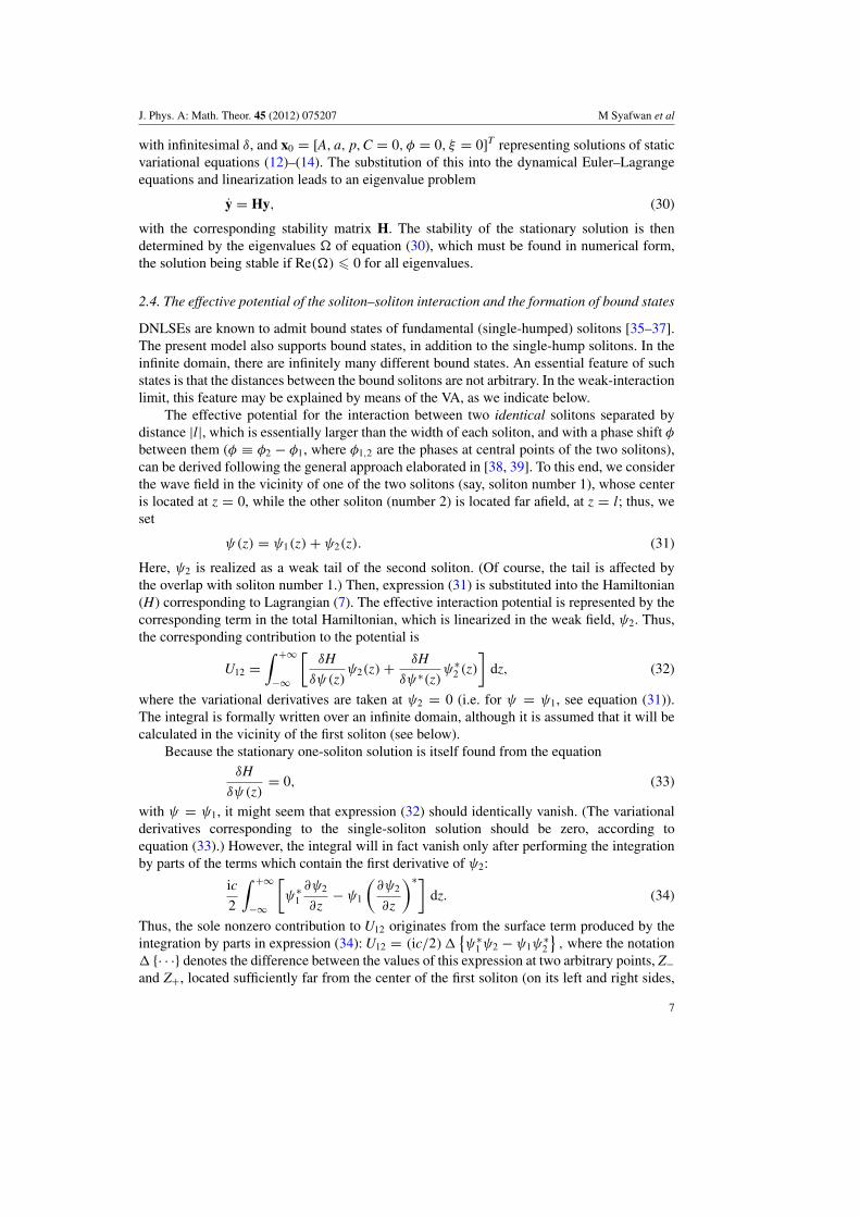
Figure 1. The comparison of two soliton profiles for two different values of �, as indicated in thecaption to each panel. The solid lines correspond to numerical results, i.e. solutions of equation(44) imposed with constraints (45), with �z = 0.2 and L = 50 (the z-axis is truncated to focus thepicture on the soliton’s core), both the real and imaginary parts being shown. The dotted lines arepredictions of the variational approximation obtained through solving equations (12)–(14).

3.1. The soliton’s core

For given parameters ε, c and �, we solve the variational equations (12)–(14) to producesuitable real solutions A, a and p, which then give a quasi-analytical approximation for thesoliton’s core described by the function ψcore(z) (see equation (8)). As generic examples,in figure 1 we present, at ε = 1 and c = 0.7, the comparison of two soliton profilesobtained from the numerical results and VA for two different values of �. We have foundA ≈ 1.228, a ≈ 0.554, p ≈ 0.377 for � = 0.5 (figure 1(a)), and A ≈ 0.685, a ≈ 0.414,

p ≈ 0.368 for � = 0.7 (figure 1(b)). Particularly good agreement is observed in both cases.To further confirm the agreement for different values of �, ε and c, in the following we

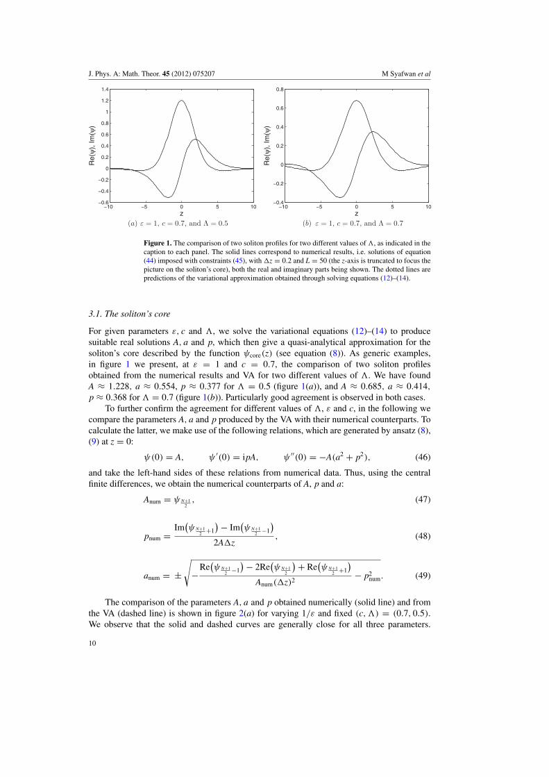
compare the parameters A, a and p produced by the VA with their numerical counterparts. Tocalculate the latter, we make use of the following relations, which are generated by ansatz (8),(9) at z = 0:

ψ(0) = A, ψ ′(0) = ipA, ψ ′′(0) = −A(a2 + p2), (46)

and take the left-hand sides of these relations from numerical data. Thus, using the centralfinite differences, we obtain the numerical counterparts of A, p and a:

Anum = ψ N+12

, (47)

pnum =Im

(ψ N+1

2 +1

) − Im(ψ N+1

2 −1

)2A�z

, (48)

anum = ±√

−Re

(ψ N+1

2 −1

) − 2Re(ψ N+1

2

) + Re(ψ N+1

2 +1

)Anum(�z)2

− p2num. (49)

The comparison of the parameters A, a and p obtained numerically (solid line) and fromthe VA (dashed line) is shown in figure 2(a) for varying 1/ε and fixed (c,�) = (0.7, 0.5).We observe that the solid and dashed curves are generally close for all three parameters.

10

J. Phys. A: Math. Theor. 45 (2012) 075207 M Syafwan et al

0.7 0.8 0.9 1 1.1 1.2 1.3 1.4 1.50.2

0.4

0.6

0.8

1

1.2

1.4

1/ε

A, a

, p

A

a

p

(a)

0.7 0.8 0.9 1 1.1 1.2 1.30.2

0.3

0.4

0.5

0.6

0.7

0.8

1/ε

A, a

, p

A

a

p

(b)

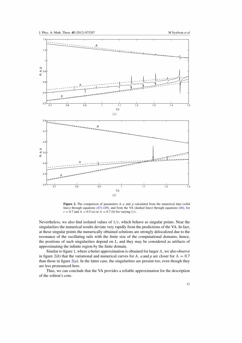
Figure 2. The comparison of parameters A, a and p calculated from the numerical data (solidlines) through equations (47)–(49), and from the VA (dashed lines) through equations (46), forc = 0.7 and � = 0.5 (a) or � = 0.7 (b) for varying 1/ε.

Nevertheless, we also find isolated values of 1/ε, which behave as singular points. Near thesingularities the numerical results deviate very rapidly from the predictions of the VA. In fact,at these singular points the numerically obtained solutions are strongly delocalized due to theresonance of the oscillating tails with the finite size of the computational domains, hence,the positions of such singularities depend on L, and they may be considered as artifacts ofapproximating the infinite region by the finite domain.

Similar to figure 1, where a better approximation is obtained for larger �, we also observein figure 2(b) that the variational and numerical curves for A, a and p are closer for � = 0.7than those in figure 2(a). In the latter case, the singularities are present too, even though theyare less pronounced here.

Thus, we can conclude that the VA provides a reliable approximation for the descriptionof the soliton’s core.

11

J. Phys. A: Math. Theor. 45 (2012) 075207 M Syafwan et al

0.7 0.8 0.9 1 1.1 1.2 1.3 1.4 1.5

−3

−2

−1

0

1

2

3

x 10−3

1/ε

Δ r

(a)

0.7 0.8 0.9 1 1.1 1.2 1.3 1.4 1.5−2

−1.8

−1.6

−1.4

−1.2

−1

−0.8

−0.6

−0.4

−0.2

0

1/ε

E

(b)

Figure 3. (a) The signed measure �r (cf equation (51)) as a function of 1/ε for c = 0.7,� = 0.5, �z = 0.2 and L = 50, where �r is zero at ε ≈ 0.737, 0.988, 1.306 (or at1/ε ≈ 1.357, 1.012, 0.766), as shown by empty circles. (b) E versus 1/ε (cf equation (23)),for the same parameter values (�, c) as in panel (a) and for the corresponding solutions for(A, a, p) and root(s) λ obtained from equations (12)–(14) and (18), respectively. It is clearly seenthat E = 0 in the observed domain of 1/ε. However, we can conjecture that ESs are located nearthe maximum of E, i.e. at ε ≈ 0.853 (or at 1/ε ≈ 1.172), as indicated by the star.

3.2. Embedded solitons

As shown in [23], in the general case the numerically obtained solitary waves are weaklydelocalized, i.e. oscillatory tails with a non-vanishing amplitude are attached to them.Nevertheless, as suggested in [22, 23], it is possible to find solutions with vanishing tails(i.e. genuine solitons) by considering quantity

�i = Im(ψ(N)), (50)

which is a signed measure, whose zeros correspond to solutions with vanishing tails. In thepresent case, the periodic boundary conditions lead to Im(ψ(N)) = 0, since the imaginarypart of ψ is odd. Therefore, we modify the signed measure (50) and redefine it as

�r = Re(ψ(N)). (51)

In figure 3(a), �r is plotted as a function of 1/ε for the parameter values (�, c,�z, L) usedin figure 2(a). We see from the figure that zeros of �r occur at ε ≈ 0.737, 0.988, 1.306

12

J. Phys. A: Math. Theor. 45 (2012) 075207 M Syafwan et al

0.7 0.8 0.9 1 1.1 1.2 1.3

−1.5

−1

−0.5

0

0.5

1

1.5

x 10−5

1/ε

Δ r

(a)

0.7 0.8 0.9 1 1.1 1.2 1.3−2

−1.8

−1.6

−1.4

−1.2

−1

−0.8

−0.6

−0.4

−0.2

0

1/ε

E

(b)

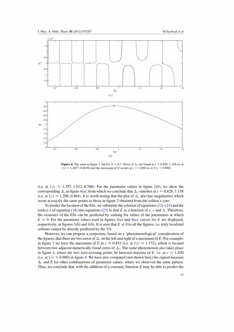
Figure 4. The same as figure 3, but for � = 0.7. Zeros of �r are found at ε ≈ 0.828, 1.158 (or at1/ε ≈ 1.2077, 0.8636) and the maximum of E occurs at ε ≈ 1.020 (or at 1/ε ≈ 0.980).

(i.e. at 1/ε ≈ 1.357, 1.012, 0.766). For the parameter values in figure 2(b), we show thecorresponding �r in figure 4(a), from which we conclude that �r vanishes at ε ≈ 0.828, 1.158(i.e. at 1/ε ≈ 1.208, 0.864). It is worth noting that the plot of �r also has singularities whichoccur at exactly the same points as those in figure 2 obtained from the soliton’s core.

To predict the location of the ESs, we substitute the solution of equations (12)–(14) and theroot(s) λ of equation (18) into equations (23) to find E as a function of ε, c and �. Therefore,the existence of the ESs can be predicted by seeking for values of the parameters at whichE = 0. For the parameter values used in figures 3(a) and 4(a), curves for E are displayed,respectively, in figures 3(b) and 4(b). It is seen that E = 0 in all the figures, i.e. truly localizedsolitons cannot be directly predicted by the VA.

However, we can propose a conjecture, based on a ‘phenomenological’ consideration ofthe figures, that there are two zeros of �r on the left and right of a maximum of E. For example,in figure 3 we have the maximum of E at ε ≈ 0.853 (i.e. at 1/ε ≈ 1.172), which is locatedbetween two adjacent numerically found zeros of �r. The same phenomenon also takes placein figure 4, where the two zero-crossing points lie between maxima of E, i.e. at ε ≈ 1.020(i.e. at 1/ε ≈ 0.980) in figure 4. We have also computed (not shown here) the signed measure�r and E for other combinations of parameter values, where we observed the same pattern.Thus, we conclude that, with the addition of a constant, function E may be able to predict the

13

J. Phys. A: Math. Theor. 45 (2012) 075207 M Syafwan et al

−200 −150 −100 −50 0 50 100 150 200

−0.4

−0.2

0

0.2

0.4

0.6

z

Re(

ψ),

Im(ψ

)

(a) |l| ≈ 39.6

−200 −150 −100 −50 0 50 100 150 200

−0.4

−0.2

0

0.2

0.4

0.6

z

Re(

ψ),

Im(ψ

)

(b) l 60.87

Figure 5. Two bound states, for ε = 0.7, c = 0.7, � = 0.7 and �z = 0.2, found numerically inthe interval of [−200, 200], for different distances between the two humps, |l|, as indicated in eachpanel. Solid and dashed lines depict Re(ψ) and Im(ψ), respectively.

location of the ESs. We suspect that the missing constant, which amounts to the shift of theplot for E vertically, is related to the choice of the ansatz (see, e.g., [42] for different ansatzeaccounting for the oscillating tails).

3.3. Stability

To determine the VA-predicted stability of the soliton, we have solved the eigenvalue problem(30). For the soliton shown in figure 1(a), i.e. with x0 ≈ [1.228, 0.554, 0.377, 0, 0, 0]T, weobtain the corresponding eigenvalues � ≈ 0, 0, 0, 0, 0.436i,−0.436i. In addition, for thesoliton in figure 1(b), i.e. x0 ≈ [0.685, 0.414, 0.368, 0, 0, 0]T, the corresponding eigenvaluesare � ≈ 0, 0, 0, 0, 0.225i,−0.225i. As the real part of all eigenvalues is zero, we concludethat both solitons are stable. These results are in agreement with the numerical findingsof [23].

3.4. Bound states

Two examples of bound states consisting of two solitons, found numerically, are presented infigure 5, each for the same parameter values.

Next, we compare the prediction presented above with the numerical results shown infigure 5. For the parameter values used in that figure, we have λr ≈ 0.441 and λi ≈ 0.505.Note that, in terms of the above analysis, the soliton centered at z = 0 in figure 5 is in factsoliton number 2. Therefore, phase difference φ in this case is calculated as the phase of thesoliton on the right minus the phase of its counterpart on the left. From the numerical results,the phase difference between the two solitons shown in the top and the bottom panels offigure 5 is given, respectively, by φ ≈ −2.012 and φ ≈ 2.368, both of which correspond tocλi/λr > 0; hence, n · sign (λi) is odd. Using equation (43), we find that the best fit to thenumerically computed distance in figure 5, i.e. |l| ≈ 39.6 and |l| ≈ 60.87, is provided by

14

J. Phys. A: Math. Theor. 45 (2012) 075207 M Syafwan et al

t

n

20 40 60 80 100

−200−150−100−50

050

100150200

−200 −150 −100 −50 0 50 100 150 2000

0.2

0.4

0.6

0.8

n

|u|

0.1

0.2

0.3

0.4

0.5

(a) l ≈ 39.6

−200 −150 −100 −50 0 50 100 150 2000

0.2

0.4

0.6

0.8

n

|u|

t

n

20 40 60 80 100

−200−150−100−50

050

100150200

0.1

0.2

0.3

0.4

0.5

(b) l 60.87

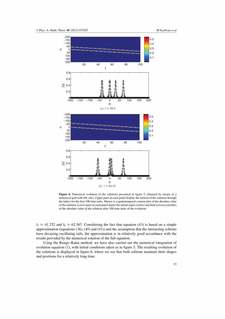
Figure 6. Numerical evolution of the solutions presented in figure 5, obtained by means of anumerical grid with 401 sites. Upper parts in each panel display the motion of the solution throughthe lattice for the first 100 time units. Shown is a spatiotemporal contour plot of the absolute valueof the solution. Lower parts in each panel depict the initial (open circles) and final (crosses) profilesof the absolute value of the solution after 100 time units of the evolution.

l7 ≈ 41.252 and l9 ≈ 62.367. Considering the fact that equation (43) is based on a simpleapproximation (equations (36), (40) and (41)) and the assumption that the interacting solitonshave decaying oscillating tails, the approximation is in relatively good accordance with theresults provided by the numerical solution of the full equation.

Using the Runge–Kutta method, we have also carried out the numerical integration ofevolution equation (1), with initial conditions taken as in figure 5. The resulting evolution ofthe solutions is displayed in figure 6, where we see that both solitons maintain their shapesand positions for a relatively long time.

15

J. Phys. A: Math. Theor. 45 (2012) 075207 M Syafwan et al

4. Conclusion

The aim of this work is to develop the semi-analytical approach to seeking traveling solitons,based on the application of the VA to the differential–difference form of the DNLSE withsaturable nonlinearity, in the moving coordinate frame. The predicted shapes of the solitonsare in good agreement with the numerical findings. The VA is also extended to examinethe stability of the traveling solitons, showing that they are stable, which is consistent withthe previous work [23]. Furthermore, the VA was developed to predict the locations of theexceptional solutions for genuine traveling solitons with strictly vanishing tails. Bound statesof two solitons were briefly considered too. In the latter case, the VA predicts the distancebetween two solitons forming the bound state. In the numerical part of the work, we havemade use of the numerical scheme for the DNLSE written in the moving coordinate frame,which is an equation of the differential–difference type. Using the Newton–Raphson method,we have confirmed the existence of exceptional solutions for traveling discrete solitons (whichare ‘embedded solitons’, in this sense), earlier predicted by means of a different numericalalgorithm. We have compared the analytical results based on the VA and the numerical findings,concluding that they are in good agreement.

Acknowledgments

MS acknowledges the Ministry of National Education of the Republic of Indonesia for financialsupport.

References

[1] Peierls R 1940 The size of a dislocation Proc. Phys. Soc. Lond. 52 34Nabarro F R N 1947 Dislocations in a simple cubic lattice Proc. Phys. Soc. Lond. 59 256

[2] Kevrekidis P G (ed) 2009 Discrete Nonlinear Schrodinger Equation: Mathematical Analysis, NumericalComputations and Physical Perspectives (New York: Springer)

[3] Lederer F, Stegeman G I, Christodoulides D N, Assanto G, Segev M and Silberberg Y 2008 Discrete solitonsin optics Phys. Rep. 463 1–126

Kartashov Y V, Vysloukh V A and Torner L 2009 Soliton shape and mobility control in optical lattices Prog.Opt. 52 63

[4] Smerzi A and Trombettoni A 2003 Nonlinear tight-binding approximation for Bose–Einstein condensates in alattice Phys. Rev. A 68 023613

Carretero-Gonzalez R, Frantzeskakis D J and Kevrekidis P G 2008 Nonlinear waves in Bose–Einsteincondensates: physical relevance and mathematical techniques Nonlinearity 21 R139

[5] Eilbeck J C 1986 Numerical simulations of the dynamics of polypeptide chains and proteins Computer Analysisfor Life Science: Progress and Challenges in Biological and Synthetic Polymer Research ed C Kawabata andA R Bishop (Tokyo: Ohmsha) pp 12–21

[6] Feddersen H 1991 Solitary wave solutions to the discrete nonlinear Schrodinger equation Nonlinear CoherentStructures in Physics and Biology (Lecture Notes in Physics vol 393) ed M Remoissenet and M Peyrard(Berlin: Springer) pp 159–67

[7] Duncan D B, Eilbeck J C, Feddersen H and Wattis J A D 1993 Solitons on lattices Physica D 68 1–11[8] Gomez-Gardenes J, Falo F and Florıa L M 2004 Mobile localization in nonlinear Schrodinger lattices Phys.

Lett. A 332 213Gomez-Gardenes J, Florıa L M, Peyrard M and Bishop A R 2004 Nonintegrable Schrodinger discrete breathers

Chaos 14 1130[9] Pelinovsky D E, Melvin T R O and Champneys A R 2007 One-parameter localized traveling waves in nonlinear

Schrodinger lattices Physica D 236 22–43[10] Melvin T R O, Champneys A R and Pelinovsky D E 2009 Discrete traveling solitons in the Salerno model SIAM

J. Appl. Dyn. Syst. 8 689–709

16

J. Phys. A: Math. Theor. 45 (2012) 075207 M Syafwan et al

[11] Fleischer J W, Segev M, Efremidis N K and Christodoulides D N 2003 Observation of two-dimensional discretesolitons in optically induced nonlinear photonic lattices Nature 422 147

[12] Neshev D, Alexander T J, Ostrovskaya E A, Kivshar Y S, Martin H, Makasyuk I and Chen Z 2004 Observationof discrete vortex solitons in optically induced photonic lattices Phys. Rev. Lett. 92 123903

Fleischer J W, Bartal G, Cohen O, Manela O, Segev M, Hudock J and Christodoulides D N 2004 Observationof vortex-ring ‘discrete’ solitons in 2D photonic lattices Phys. Rev. Lett. 92 123904

[13] Yang J, Makasyuk I, Kevrekidis P G, Martin H, Malomed B A, Frantzeskakis D J and Chen Z G 2005 Necklace-like solitons in optically induced photonic lattices Phys. Rev. Lett. 94 113902

[14] Wang X S, Chen Z G and Kevrekidis P G 2006 Observation of discrete solitons and soliton rotation in opticallyinduced periodic ring lattices Phys. Rev. Lett. 96 083904

[15] Kevrekidis P G, Chen Z G, Malomed B A, Frantzeskakis D J and Weinstein M I 2005 Spontaneous symmetrybreaking in photonic lattices: theory and experiment Phys. Lett. A 340 275–80

[16] Sakaguchi H and Malomed B A 2005 Higher-order vortex solitons, multipoles and supervortices on a squareoptical lattice Europhys. Lett. 72 698–704

Kevrekidis P G, Susanto H and Chen Z 2006 High-order-mode soliton structures in two-dimensional latticeswith defocusing nonlinearity Phys. Rev. E 74 066606

[17] Carretero-Gonzalez R, Talley J D, Chong C and Malomed B A 2006 Multistable solitons in the cubic–quinticdiscrete nonlinear Schrodinger equation Physica D 216 77–89

Chong C, Carretero-Gonzalez R, Malomed B A and Kevrekidis P G 2009 Multistable solitons in higher-dimensional cubic–quintic nonlinear Schrodinger lattices Physica D 238 126–36

[18] Vicencio R A and Johansson M 2006 Discrete soliton mobility in two-dimensional waveguide arrays withsaturable nonlinearity Phys. Rev. E 73 046602

[19] Hadzievski L, Maluckov A, Stepic M and Kip D 2004 Power controlled soliton stability and steering in latticeswith saturable nonlinearity Phys. Rev. Lett. 93 033901

[20] Khare A, Rasmussen K Ø, Samuelsen M R and Saxena A 2005 J. Phys. A: Math. Gen. 38 807[21] Khare A, Rasmussen K Ø, Samuelsen M R and Saxena A 2009 J. Phys. A: Math. Theor. 42 085002[22] Melvin T R O, Champneys A R, Kevrekidis P G and Cuevas J 2006 Radiationless travelling waves in saturable

nonlinear Schrodinger lattices Phys. Rev. Lett. 97 124101[23] Melvin T R O, Champneys A R, Kevrekidis P G and Cuevas J 2008 Travelling solitary waves in the

discrete Schrodinger equation with saturable nonlinearity: existence, stability and dynamics PhysicaD 237 551–67

[24] Yang J, Malomed B A and Kaup D J 1999 Embedded solitons in second-harmonic-generating systems Phys.Rev. Lett. 83 1958–61

Champneys A R, Malomed B A, Yang J and Kaup D J 2001 ‘Embedded solitons’: solitary waves in resonancewith the linear spectrum Physica D 152–153 340–54

[25] Champneys A R and Malomed B A 1999 Moving embedded solitons J. Phys. A: Math. Gen. 32 L547–53[26] Gonzalez-Perez-Sandi S, Fujioka J and Malomed B A 2004 Embedded solitons in dynamical lattices Physica

D 197 86–100Yagasaki K, Champneys A R and Malomed B A 2005 Discrete embedded solitons Nonlinearity 18 2591–613Malomed B A, Fujioka J, Espinosa-Ceron A, Rodriguez R F and Gonzalez S 2006 Moving embedded lattice

solitons Chaos 16 013112[27] Oxtoby O F and Barashenkov I V 2007 Moving solitons in the discrete nonlinear Schrodinger equation Phys.

Rev. E 76 036603[28] Malomed B A and Weinstein M I 1996 Soliton dynamics in the discrete nonlinear Schrodinger equation Phys.

Lett. A 220 91–6[29] Kaup D J 2005 Variational solutions for the discrete nonlinear Schrodinger equation Math. Comput.

Simul. 69 322–33[30] Chong C and Pelinovsky D E 2011 Variational approximations of bifurcations of asymmetric solitons in cubic–

quintic nonlinear Schrodinger lattices Discrete Control Dyn. Syst. S 4 1019–32[31] Chong C, Pelinovsky D E and Schneider G 2011 On the validity of the variational approximation in discrete

nonlinear Schrodinger equations Physica D 241 115–24[32] Kaup D J and Malomed B A 2003 Embedded solitons in Lagrangian and semi-Lagrangian systems Physica

D 184 153–61[33] Gradshteyn I S and Ryzhik I M 2000 Tables of Integrals, Series and Products (New York: Academic)[34] Flytzanis N, Malomed B A and Wattis J A D 1993 Analysis of stability of solitons in one-dimensional lattices

Phys. Lett. A 180 107–12[35] Kivshar Y S, Champneys A R, Cai D and Bishop A R 1998 Multiple states of intrinsic localized modes Phys.

Rev. B 58 5423–8

17

J. Phys. A: Math. Theor. 45 (2012) 075207 M Syafwan et al

[36] Kapitula T, Kevrekidis P G and Malomed B A 2001 Stability of multiple pulses in discrete systems Phys. Rev.E 63 036604

[37] Kevrekidis P G 2001 Multipulses in discrete Hamiltonian nonlinear systems Phys. Rev. E 64 026611[38] Malomed B A and Nepomnyashchy A A 1994 Stability limits for arrays of kinks in two-component nonlinear

systems Europhys. Lett. 27 649[39] Malomed B A 1998 Potential of interaction between two- and three-dimensional solitons Phys. Rev. E 58 7928[40] Weideman J and Reddy S 2000 A MATLAB differentiation matrix suite ACM Trans. Math. Softw. 26 465–519[41] Trefethen L N 2000 Spectral Methods in MATLAB (Philadelphia, PA: SIAM)[42] Boyd J P 1998 Weakly Nonlocal Solitary Waves and Beyond-all-orders Asymptotics (Dordrecht: Kluwer)

18