arX

iv:n

lin/0

3030

25v1

[nl

in.S

I] 1

4 M

ar 2

003

Exact soliton solutions of coupled nonlinear Schrodinger

equations: Shape changing collisions, logic gates and partially

coherent solitons

T. Kanna and M. Lakshmanan∗

Centre for Nonlinear Dynamics, Department of Physics,

Bharathidasan University, Tiruchirapalli 620 024, India

1

Abstract

The novel dynamical features underlying soliton interactions in coupled nonlinear Schrodinger

equations, which model multimode wave propagation under varied physical situations in nonlinear

optics, are studied. In this paper, by explicitly constructing multisoliton solutions (upto four-soliton

solutions) for two coupled and arbitrary N -coupled nonlinear Schrodinger equations using the

Hirota bilinearization method, we bring out clearly the various features underlying the fascinating

shape changing (intensity redistribution) collisions of solitons, including changes in amplitudes,

phases and relative separation distances, and the very many possibilities of energy redistributions

among the modes of solitons. However in this multisoliton collision process the pair-wise collision

nature is shown to be preserved in spite of the changes in the amplitudes and phases of the solitons.

Detailed asymptotic analysis also shows that when solitons undergo multiple collisions, there exists

the exciting possibility of shape restoration of atleast one soliton during interactions of more than

two solitons represented by three and higher order soliton solutions. From application point of

view, we have shown from the asymptotic expressions how the amplitude (intensity) redistribution

can be written as a generalized linear fractional transformation for the N -component case. Also we

indicate how the multisolitons can be reinterpreted as various logic gates for suitable choices of the

soliton parameters, leading to possible multistate logic. In addition, we point out that the various

recently studied partially coherent solitons are just special cases of the bright soliton solutions

exhibiting shape changing collisions, thereby explaining their variable profile and shape variation

in collision process.

PACS numbers: 42.81.Dp, 42.65.Tg, 05.45.Yv

∗Electronic address: cnld123@eth.net

2

I. INTRODUCTION

The study of coupled nonlinear Schrodinger (CNLS) equations is receiving a great deal of

attention in recent years due to their appearance as modelling equations in diverse areas of

physics like nonlinear optics [1], including optical communications [2], bio-physics [3], mul-

ticomponent Bose-Einstein condensates at zero temperature [4], etc. To be specific, soliton

type pulse propagation in multimode fibers [1] and in fiber arrays [5] is governed by a set of

N -CNLS equations which is not integrable in general. However, it becomes integrable for

specific choice of parameters [6,7]. On the other hand, the recent studies on the coherent

[8] and incoherent [9] beam propagation in photorefractive media, which can exhibit high

nonlinearity with extremely low optical power, necessitate intense study of CNLS equations

both integrable and nonintegrable. The first experimental observation of the so-called par-

tially incoherent solitons with the excitation of a light bulb in a photorefractive medium

[10] has made this study even more interesting. In this context of beam propagation in a

Kerr like photorefractive medium, the governing equations are a set of N -CNLS equations

[11,12].

We consider the following N -CNLS equations of Manakov type [13] for our study,

iqjz + qjtt + 2µ

N∑

p=1

|qp|2qj = 0, j = 1, 2, ..., N, (1)

where qj is the envelope in the jth mode, z and t represent the normalized distance along the

fiber and the retarded time respectively, in the context of soliton propagation in multimode

fibers. In the case of fiber arrays qj corresponds to the jth core. Here 2µ gives the strength

of the nonlinearity. In the framework of N self trapped mutually incoherent wavepackets

propagation in Kerr-like photorefractive media [11,12], qj is the jth component of the beam,

z and t represent the coordinates along the direction of propagation and the transverse

coordinate, respectively. The interesting property of the N -CNLS equations of the form (1)

is that they are integrable equations and possess soliton solutions.

It is obvious from Eq. (1) that for N = 1 it corresponds to the standard envelope soliton

possessing integrable nonlinear Schrodinger equation, governing intense optical pulse propa-

gation through single mode optical fiber [1,14]. For N = 2 case, it reduces to the celebrated

Manakov model [13] describing intense electromagnetic pulse propagation in birefringent

fiber. Manakov himself has made a detailed asymptotic analysis of the inverse scattering

3

problem associated with the system (1) for N = 2 and identified changes in the polariza-

tion vector [13]. However no explicit two soliton expression was given there. Very recently,

Radhakrishnan, Lakshmanan and Hietarinta have obtained the bright one- and two-soliton

solutions for this case [15] and have revealed certain novel shape changing (intensity re-

distribution) collision properties. These Manakov solitons have been observed recently in

AlGaAs planar waveguides [16] and precisely this kind of energy exchanging (shape chang-

ing) collisions has been experimentally demonstrated in [17]. The results of Ref. [15] have

led Jakubowski, Squier and Steiglitz [18] to express the energy redistributions as linear

fractional transformations so as to construct logic gates. Later, Steiglitz [19] explicitly con-

structed such logic gates including the universal NAND gate, based on the shape changing

collision property, and hence pointed out the possibility of designing an all optical computer

equivalent to a Turing machine, at least in a mathematical sense. However, results are scarce

for N ≥ 2 case of Eq. (1) though they are of considerable physical importance as mentioned

earlier.

The novel shape changing collision property exhibited by the 2-CNLS equations, which

has not been observed in general in any other simpler (1+1) dimensional integrable system,

requires a detailed analysis to identify the various possibilities and the underlying potential

technological applications. In a very recent letter [20], the present authors have studied the

multicomponent N-CNLS equations and shown that shape changing collisions occur here also

with more possibilities of energy redistribution. It has also been briefly pointed out that

the much discussed partially coherent solitons (PCSs) [11,12], which are of variable shape,

namely 2-PCS, 3-PCS,..., N -PCS, are special cases of the 2-soliton, 3-soliton,..., N -soliton

solutions of the 2-CNLS, 3-CNLS,..., N -CNLS equations, respectively. The understanding of

variable shapes [11,12] of these recently experimentally observed partially coherent solitons

[21] in photorefractive medium and their interesting collision behaviour will be fascilitated

by obtaining the higher order soliton solutions of the 2-CNLS and the N -CNLS (N≥ 2)

equations.

In this paper, we wish to undertake a detailed analysis of the dynamical features associ-

ated with soliton interactions in multicomponent N -CNLS equations. There exists numerous

interesting phenomena which one has to pay attention in order to realize the full potential-

ities of these equations and the underlying novel soliton dynamics. Some of the important

aspects include the following among others:

4

1. Explicit expressions for multisoliton solutions in multicomponent CNLS equations use-

ful for analysis of interactions (as against formal expressions).

2. Novel soliton interactions involving shape changing collisions.

3. Dependence of shape changes and relative separation distances on amplitudes of the

colliding solitons.

4. Identification of different possibilities of energy redistributions among the different

modes of the soliton during collision and obtaining generalized linear fractional trans-

formations.

5. State restoring properties in multisoliton solutions.

6. Existence of partially coherent solitons, stationary and moving, as special cases of the

above multisoliton solutions.

7. Identification of multisoliton solutions as logic gates in multicomponent CNLS equa-

tions.

The present paper will be essentially devoted to the understanding of multisoliton inter-

actions in N-CNLS equations, and its application in constructing logic gates and in iden-

tifying partially coherent solitons as special cases of multisoliton solutions. In particular,

in the present paper, we will deduce explicit expressions for multisoliton solutions (upto

four-soliton solution), which can be easily generalized to arbitrary soliton case, 2-CNLS and

then for arbitrary N -CNLS equations. To start with, we will briefly consider the two-soliton

solution to bring out the shape changing nature of soliton collisions, which can be quantified

in terms of generalized linear fractional transformations (LFTs), and identify the changes

in amplitudes, phases and relative separation distances among the solitons by carrying out

appropriate asymptotic analysis. However the standard (shape preserving) elastic collisions

can occur for specific choice of soliton parameters (initial conditions). More interestingly, we

also point out that when more than two solitons collide successively, say three solitons, there

exists the exciting possibility of restoration of the shape of one of the three solitons leaving

the other two undergoing shape changes and we prove that the underlying soliton interac-

tion is pair-wise. We give explicit conditions for the shape restoring property. Extending

this analysis, one can easily check that in an M-soliton collision, it is possible to restore

5

the states of (M − 2) solitons after collisions. Such possibilities lead to the construction of

optical logic gates of different types and generalized linear fractional transformations, as we

will show in this manuscript.

This paper is organized as follows. In Sec. II we briefly present the bilinearization

procedure for the N -CNLS equations. Explicit multisoliton solutions (upto four) of the

2-CNLS equations are obtained in Sec. III. Then the generalization of these multisoliton

solutions to N -CNLS equations is given in Sec. IV. The two soliton collision properties of

2-CNLS and their generalization to N -CNLS equations are studied in Sec. V. In Sec. VI,

we present a systematic procedure to identify the intensity redistribution among N modes

in terms of a generalized linear fractional transformation which is the precursor to develop

logic gates without interconnecting discrete components [18]. The interesting feature of

the higher order soliton solutions, namely the pair-wise nature of collision of solitons, and

the shape restoration property of the state of one soliton only in a three soliton collision

process are presented in Sec. VII. In Sec. VIII we introduce the possibility of looking at

the bright soliton solutions as logic gates, as an alternate point of view. Then in Sec. IX

we demonstrate explicitly that for specific choices of the parameters of the bright soliton

solutions various PCSs reported in the literature result. The collision properties of PCSs

and the salient features of multisoliton complexes are also discussed. Sec. X is allotted for

conclusion. Also in Appendix A we present the explicit form of the four-soliton solution.

II. BILINEARIZATION

The set of N -CNLS equations (1) has been found to be completely integrable [6,7] and

admits exact bright soliton solutions. Their explicit forms can be obtained by using the

Hirota’s bilinearization method [22], which is straightforward. Any of the other soliton pro-

ducing methodologies in principle is equally applicable, however, this paper is not concerned

with the relative merits of the various methodologies.

To start with, we make the bilinearizing transformation (which can be identified system-

atically from the Laurent expansion [6])

qj =g(j)

f, j = 1, 2, ..., N, (2)

6

to Eq. (1). This results in the following set of bilinear equations,

(iDz + D2t )g

(j).f = 0, j = 1, 2, ..., N, (3a)

D2t f.f = 2µ

N∑

n=1

g(n)g(n)∗, (3b)

where ∗ denotes the complex conjugate, g(j)’s are complex functions, while f(z, t) is a real

function and the Hirota’s bilinear operators Dz and Dt are defined by

Dnz Dm

t (a.b) =

(

∂

∂z− ∂

∂z′

)n (

∂

∂t− ∂

∂t′

)m

a(z, t)b(z′, t′)∣

∣

∣

(z=z′,t=t′). (3c)

The above set of equations can be solved by introducing the following power series expansions

for g(j)’s and f :

g(j) = χg(j)1 + χ3g

(j)3 + ..., j = 1, 2, ..., N, (4a)

f = 1 + χ2f2 + χ4f4 + ..., (4b)

where χ is the formal expansion parameter. The resulting set of equations, after collecting

the terms with the same power in χ, can be solved recursively to obtain the forms of g(j)’s

and f . Though a formal closed form solution of the N -soliton expression of Eq. (1) as a

ratio of two (N × N) determinants can be given [23], it becomes necessary to deduce the

explicit expressions (which is nontrivial) in order to understand the interaction properties

at least for the lower order solitons. In the next section we will only present the minimum

details.

III. MULTISOLITON SOLUTIONS FOR N = 2 CASE

As a prelude to understand the nature of soliton solutions for arbitrary N -CNLS equa-

tions, we first present the bright one- and two- soliton solutions of Eq. (1) with N=2

(Manakov) case as given in Ref. [15] and then extend the analysis to obtain the explicit

higher order soliton solutions.

A. One-soliton solution

After restricting the power series expansion (4) as

g(j) = χg(j)1 , j = 1, 2, f = 1 + χ2f2, (5)

7

and solving the resulting set of linear partial differential equations recursively, one can write

down the explicit one-soliton solution as

q1

q2

=

α(1)1

α(2)1

eη1

1 + eη1+η∗

1+R=

A1

A2

k1Reiη1I

cosh (η1R + R2), (6)

where η1 = k1(t + ik1z), Aj =α

(j)1

[

µ(

|α(1)1 |2+|α

(2)1 |2

)]1/2 , j = 1, 2, and eR =µ(

|α(1)1 |2+|α

(2)1 |2

)

(k1+k∗

1)2. Note

that this one-soliton solution is characterized by three arbitrary complex parameters α(1)1 ,

α(2)1 , and k1. Here the amplitude of the soliton in the first and second components (modes)

are given by k1RA1 and k1RA2, respectively, subject to the condition |A1|2 + |A2|2 = 1µ,

while the soliton velocity in both the modes is given by 2k1I . Here k1R and k1I represent

the real and imaginary parts of the complex parameter k1. The quantity R2k1R

= 12k1R

log

[

µ(

|α(1)1 |2+|α

(2)1 |2

)

(k1+k∗

1)2

]

denotes the position of the soliton.

B. Two-soliton solution

The two-soliton solution of the integrable 2-CNLS system has been obtained in Ref. [15]

after terminating the power series (4) as

g(j) = χg(j)1 + χ3g

(j)3 , j = 1, 2, (7a)

f = 1 + χ2f2 + χ4f4, (7b)

and again solving the resultant linear partial differential equations recursively . Then the

explicit form of the two-soliton solution can be written as

qj =α

(j)1 eη1 + α

(j)2 eη2 + eη1+η∗

1+η2+δ1j + eη1+η2+η∗

2+δ2j

D, j = 1, 2, (8a)

where

D = 1 + eη1+η∗

1+R1 + eη1+η∗

2+δ0 + eη∗

1+η2+δ∗0 + eη2+η∗

2+R2 + eη1+η∗

1+η2+η∗

2+R3 . (8b)

In Eqs. (8), we have defined

ηi = ki(t + ikiz), eδ0 =κ12

k1 + k∗2

, eR1 =κ11

k1 + k∗1

, eR2 =κ22

k2 + k∗2

,

eδ1j =(k1 − k2)(α

(j)1 κ21 − α

(j)2 κ11)

(k1 + k∗1)(k

∗1 + k2)

, eδ2j =(k2 − k1)(α

(j)2 κ12 − α

(j)1 κ22)

(k2 + k∗2)(k1 + k∗

2),

eR3 =|k1 − k2|2

(k1 + k∗1)(k2 + k∗

2)|k1 + k∗2|2

(κ11κ22 − κ12κ21), (8c)

8

and

κil =µ

∑2n=1 α

(n)i α

(n)∗l

(ki + k∗l )

, i, l = 1, 2. (8d)

The above most general bright two-soliton solution is characterized by six arbitrary complex

parameters k1, k2, α(j)1 , and α

(j)2 , j = 1, 2, and it corresponds to the collision of two bright

solitons. Note that in Ref. [15], δ11, δ12, δ21, and δ22 are called as δ1, δ′1, δ2, and δ′2,

respectively. The redefined quantities δij ’s, i, j = 1, 2, are now used for notational simplicity.

C. Three-soliton solution

The two-soliton solution itself is very difficult to derive and complicated to analyse [15].

So obtaining the three-soliton solution is a more laborious and tedious task. However we

have successfully obtained the explicit form of the bright three-soliton solution also. In order

to obtain the three-soliton solution of Eq. (1) for the N = 2 case we terminate the power

series (4a) and (4b) as

g(j) = χg(j)1 + χ3g

(j)3 + χ5g

(j)5 , (9a)

f = 1 + χ2f2 + χ4f4 + χ6f6, j = 1, 2. (9b)

Substitution of (9) into the bilinear Eqs. (3a) and (3b) yields a set of linear partial differential

equations at various powers of χ . The three-soliton solution consistent with these equations

is

qj =α

(j)1 eη1 + α

(j)2 eη2 + α

(j)3 eη3 + eη1+η∗

1+η2+δ1j + eη1+η∗

1+η3+δ2j + eη2+η∗

2+η1+δ3j

D

+eη2+η∗

2+η3+δ4j + eη3+η∗

3+η1+δ5j + eη3+η∗

3+η2+δ6j + eη∗

1+η2+η3+δ7j + eη1+η∗

2+η3+δ8j

D

+eη1+η2+η∗

3+δ9j + eη1+η∗

1+η2+η∗

2+η3+τ1j + eη1+η∗

1+η3+η∗

3+η2+τ2j

D

+eη2+η∗

2+η3+η∗

3+η1+τ3j

D, j = 1, 2, (10a)

9

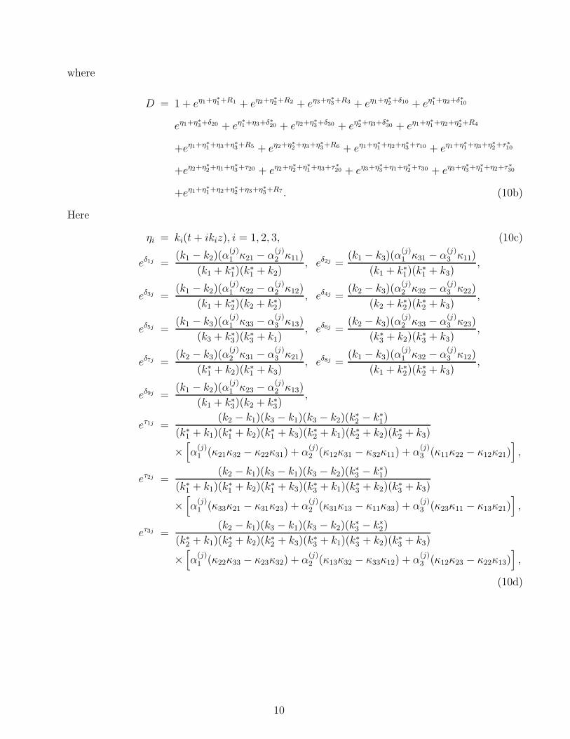
where

D = 1 + eη1+η∗

1+R1 + eη2+η∗

2+R2 + eη3+η∗

3+R3 + eη1+η∗

2+δ10 + eη∗

1+η2+δ∗10

eη1+η∗

3+δ20 + eη∗

1+η3+δ∗20 + eη2+η∗

3+δ30 + eη∗

2+η3+δ∗30 + eη1+η∗

1+η2+η∗

2+R4

+eη1+η∗

1+η3+η∗

3+R5 + eη2+η∗

2+η3+η∗

3+R6 + eη1+η∗

1+η2+η∗

3+τ10 + eη1+η∗

1+η3+η∗

2+τ∗

10

+eη2+η∗

2+η1+η∗

3+τ20 + eη2+η∗

2+η∗

1+η3+τ∗

20 + eη3+η∗

3+η1+η∗

2+τ30 + eη3+η∗

3+η∗

1+η2+τ∗

30

+eη1+η∗

1+η2+η∗

2+η3+η∗

3+R7 . (10b)

Here

ηi = ki(t + ikiz), i = 1, 2, 3, (10c)

eδ1j =(k1 − k2)(α

(j)1 κ21 − α

(j)2 κ11)

(k1 + k∗1)(k

∗1 + k2)

, eδ2j =(k1 − k3)(α

(j)1 κ31 − α

(j)3 κ11)

(k1 + k∗1)(k

∗1 + k3)

,

eδ3j =(k1 − k2)(α

(j)1 κ22 − α

(j)2 κ12)

(k1 + k∗2)(k2 + k∗

2), eδ4j =

(k2 − k3)(α(j)2 κ32 − α

(j)3 κ22)

(k2 + k∗2)(k

∗2 + k3)

,

eδ5j =(k1 − k3)(α

(j)1 κ33 − α

(j)3 κ13)

(k3 + k∗3)(k

∗3 + k1)

, eδ6j =(k2 − k3)(α

(j)2 κ33 − α

(j)3 κ23)

(k∗3 + k2)(k∗

3 + k3),

eδ7j =(k2 − k3)(α

(j)2 κ31 − α

(j)3 κ21)

(k∗1 + k2)(k∗

1 + k3), eδ8j =

(k1 − k3)(α(j)1 κ32 − α

(j)3 κ12)

(k1 + k∗2)(k

∗2 + k3)

,

eδ9j =(k1 − k2)(α

(j)1 κ23 − α

(j)2 κ13)

(k1 + k∗3)(k2 + k∗

3),

eτ1j =(k2 − k1)(k3 − k1)(k3 − k2)(k

∗2 − k∗

1)

(k∗1 + k1)(k∗

1 + k2)(k∗1 + k3)(k∗

2 + k1)(k∗2 + k2)(k∗

2 + k3)

×[

α(j)1 (κ21κ32 − κ22κ31) + α

(j)2 (κ12κ31 − κ32κ11) + α

(j)3 (κ11κ22 − κ12κ21)

]

,

eτ2j =(k2 − k1)(k3 − k1)(k3 − k2)(k

∗3 − k∗

1)

(k∗1 + k1)(k∗

1 + k2)(k∗1 + k3)(k∗

3 + k1)(k∗3 + k2)(k∗

3 + k3)

×[

α(j)1 (κ33κ21 − κ31κ23) + α

(j)2 (κ31κ13 − κ11κ33) + α

(j)3 (κ23κ11 − κ13κ21)

]

,

eτ3j =(k2 − k1)(k3 − k1)(k3 − k2)(k

∗3 − k∗

2)

(k∗2 + k1)(k∗

2 + k2)(k∗2 + k3)(k∗

3 + k1)(k∗3 + k2)(k∗

3 + k3)

×[

α(j)1 (κ22κ33 − κ23κ32) + α

(j)2 (κ13κ32 − κ33κ12) + α

(j)3 (κ12κ23 − κ22κ13)

]

,

(10d)

10

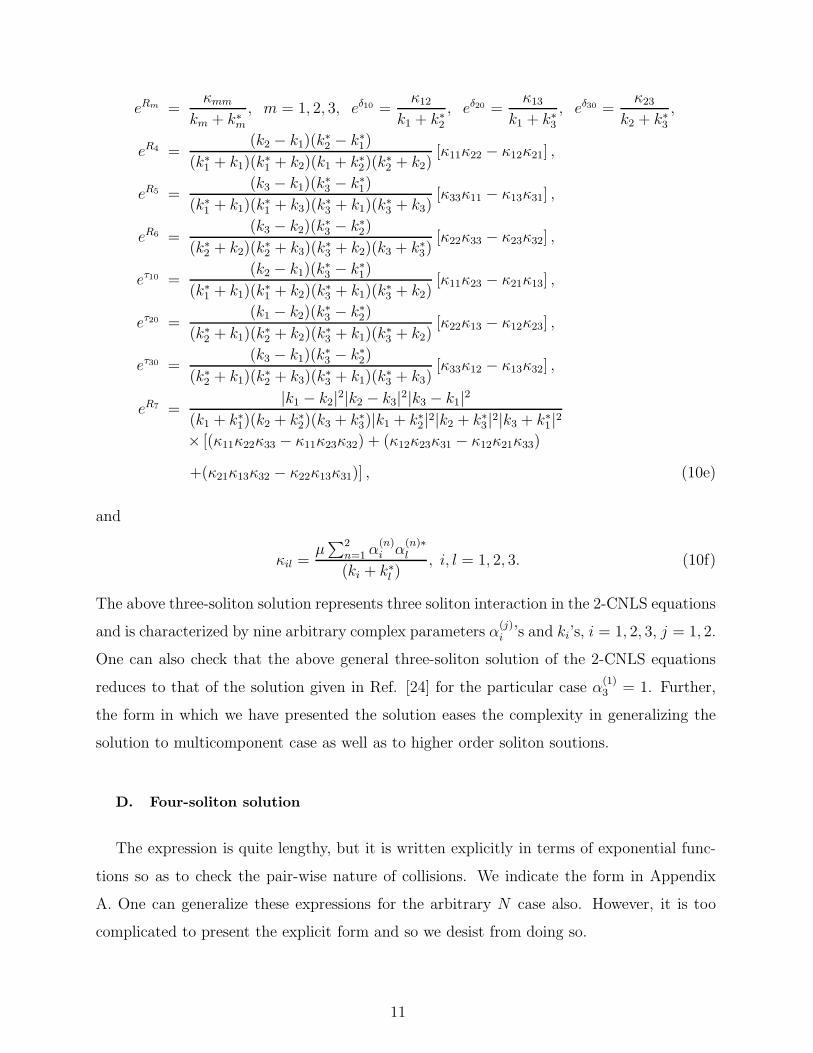
eRm =κmm

km + k∗m

, m = 1, 2, 3, eδ10 =κ12

k1 + k∗2

, eδ20 =κ13

k1 + k∗3

, eδ30 =κ23

k2 + k∗3

,

eR4 =(k2 − k1)(k

∗2 − k∗

1)

(k∗1 + k1)(k∗

1 + k2)(k1 + k∗2)(k

∗2 + k2)

[κ11κ22 − κ12κ21] ,

eR5 =(k3 − k1)(k

∗3 − k∗

1)

(k∗1 + k1)(k∗

1 + k3)(k∗3 + k1)(k∗

3 + k3)[κ33κ11 − κ13κ31] ,

eR6 =(k3 − k2)(k

∗3 − k∗

2)

(k∗2 + k2)(k∗

2 + k3)(k∗3 + k2)(k3 + k∗

3)[κ22κ33 − κ23κ32] ,

eτ10 =(k2 − k1)(k

∗3 − k∗

1)

(k∗1 + k1)(k

∗1 + k2)(k

∗3 + k1)(k

∗3 + k2)

[κ11κ23 − κ21κ13] ,

eτ20 =(k1 − k2)(k

∗3 − k∗

2)

(k∗2 + k1)(k∗

2 + k2)(k∗3 + k1)(k∗

3 + k2)[κ22κ13 − κ12κ23] ,

eτ30 =(k3 − k1)(k

∗3 − k∗

2)

(k∗2 + k1)(k

∗2 + k3)(k

∗3 + k1)(k

∗3 + k3)

[κ33κ12 − κ13κ32] ,

eR7 =|k1 − k2|2|k2 − k3|2|k3 − k1|2

(k1 + k∗1)(k2 + k∗

2)(k3 + k∗3)|k1 + k∗

2|2|k2 + k∗3|2|k3 + k∗

1|2× [(κ11κ22κ33 − κ11κ23κ32) + (κ12κ23κ31 − κ12κ21κ33)

+(κ21κ13κ32 − κ22κ13κ31)] , (10e)

and

κil =µ

∑2n=1 α

(n)i α

(n)∗l

(ki + k∗l )

, i, l = 1, 2, 3. (10f)

The above three-soliton solution represents three soliton interaction in the 2-CNLS equations

and is characterized by nine arbitrary complex parameters α(j)i ’s and ki’s, i = 1, 2, 3, j = 1, 2.

One can also check that the above general three-soliton solution of the 2-CNLS equations

reduces to that of the solution given in Ref. [24] for the particular case α(1)3 = 1. Further,

the form in which we have presented the solution eases the complexity in generalizing the

solution to multicomponent case as well as to higher order soliton soutions.

D. Four-soliton solution

The expression is quite lengthy, but it is written explicitly in terms of exponential func-

tions so as to check the pair-wise nature of collisions. We indicate the form in Appendix

A. One can generalize these expressions for the arbitrary N case also. However, it is too

complicated to present the explicit form and so we desist from doing so.

11

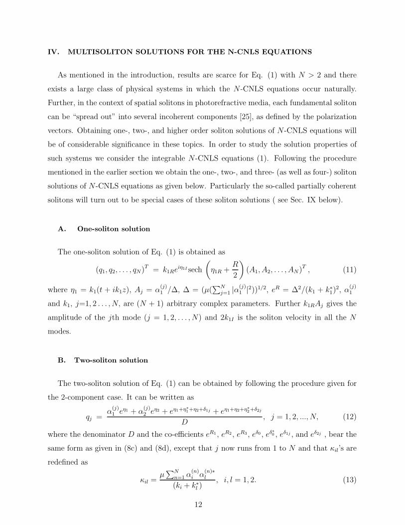
IV. MULTISOLITON SOLUTIONS FOR THE N-CNLS EQUATIONS

As mentioned in the introduction, results are scarce for Eq. (1) with N > 2 and there

exists a large class of physical systems in which the N -CNLS equations occur naturally.

Further, in the context of spatial solitons in photorefractive media, each fundamental soliton

can be “spread out” into several incoherent components [25], as defined by the polarization

vectors. Obtaining one-, two-, and higher order soliton solutions of N -CNLS equations will

be of considerable significance in these topics. In order to study the solution properties of

such systems we consider the integrable N -CNLS equations (1). Following the procedure

mentioned in the earlier section we obtain the one-, two-, and three- (as well as four-) soliton

solutions of N -CNLS equations as given below. Particularly the so-called partially coherent

solitons will turn out to be special cases of these soliton solutions ( see Sec. IX below).

A. One-soliton solution

The one-soliton solution of Eq. (1) is obtained as

(q1, q2, . . . , qN)T = k1Reiη1I sech

(

η1R +R

2

)

(A1, A2, . . . , AN)T , (11)

where η1 = k1(t + ik1z), Aj = α(j)1 /∆, ∆ = (µ(

∑Nj=1 |α

(j)1 |2))1/2, eR = ∆2/(k1 + k∗

1)2, α

(j)1

and k1, j=1, 2 . . . , N, are (N + 1) arbitrary complex parameters. Further k1RAj gives the

amplitude of the jth mode (j = 1, 2, . . . , N) and 2k1I is the soliton velocity in all the N

modes.

B. Two-soliton solution

The two-soliton solution of Eq. (1) can be obtained by following the procedure given for

the 2-component case. It can be written as

qj =α

(j)1 eη1 + α

(j)2 eη2 + eη1+η∗

1+η2+δ1j + eη1+η2+η∗

2+δ2j

D, j = 1, 2, ..., N, (12)

where the denominator D and the co-efficients eR1 , eR2 , eR3 , eδ0 , eδ∗0 , eδ1j , and eδ2j , bear the

same form as given in (8c) and (8d), except that j now runs from 1 to N and that κil’s are

redefined as

κil =µ

∑Nn=1 α

(n)i α

(n)∗l

(ki + k∗l )

, i, l = 1, 2. (13)

12

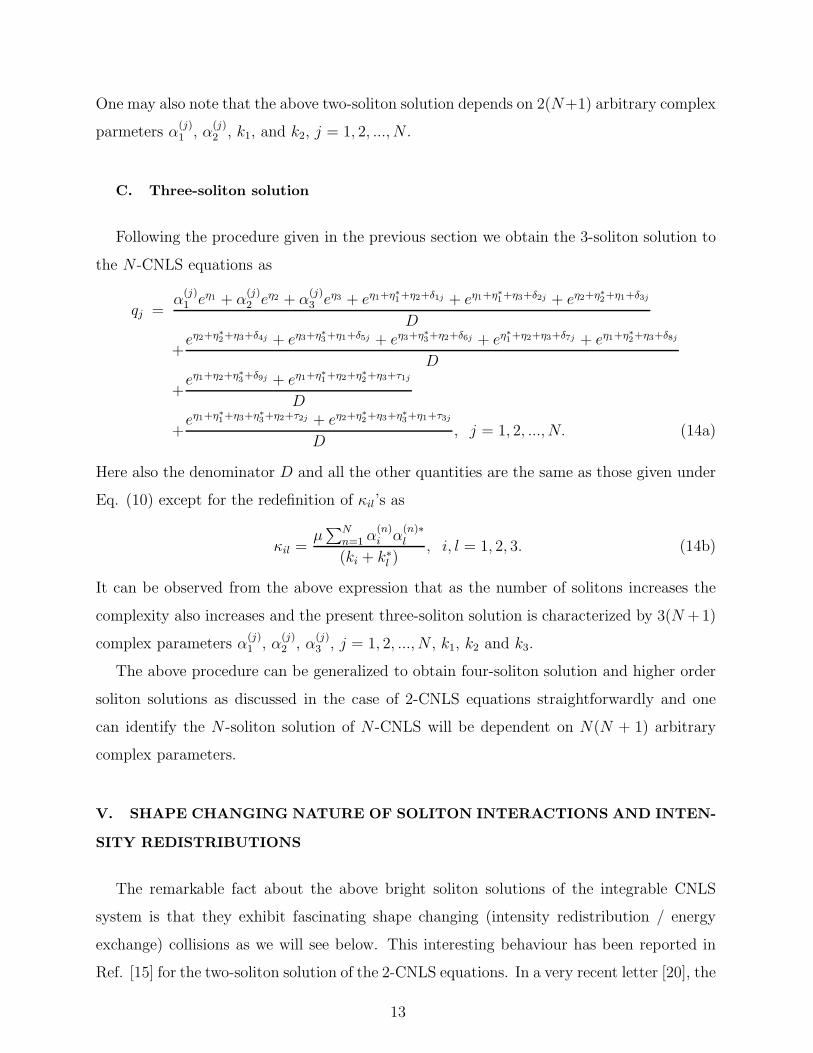
One may also note that the above two-soliton solution depends on 2(N+1) arbitrary complex

parmeters α(j)1 , α

(j)2 , k1, and k2, j = 1, 2, ..., N .

C. Three-soliton solution

Following the procedure given in the previous section we obtain the 3-soliton solution to

the N -CNLS equations as

qj =α

(j)1 eη1 + α

(j)2 eη2 + α

(j)3 eη3 + eη1+η∗

1+η2+δ1j + eη1+η∗

1+η3+δ2j + eη2+η∗

2+η1+δ3j

D

+eη2+η∗

2+η3+δ4j + eη3+η∗

3+η1+δ5j + eη3+η∗

3+η2+δ6j + eη∗

1+η2+η3+δ7j + eη1+η∗

2+η3+δ8j

D

+eη1+η2+η∗

3+δ9j + eη1+η∗

1+η2+η∗

2+η3+τ1j

D

+eη1+η∗

1+η3+η∗

3+η2+τ2j + eη2+η∗

2+η3+η∗

3+η1+τ3j

D, j = 1, 2, ..., N. (14a)

Here also the denominator D and all the other quantities are the same as those given under

Eq. (10) except for the redefinition of κil’s as

κil =µ

∑Nn=1 α

(n)i α

(n)∗l

(ki + k∗l )

, i, l = 1, 2, 3. (14b)

It can be observed from the above expression that as the number of solitons increases the

complexity also increases and the present three-soliton solution is characterized by 3(N +1)

complex parameters α(j)1 , α

(j)2 , α

(j)3 , j = 1, 2, ..., N , k1, k2 and k3.

The above procedure can be generalized to obtain four-soliton solution and higher order

soliton solutions as discussed in the case of 2-CNLS equations straightforwardly and one

can identify the N -soliton solution of N -CNLS will be dependent on N(N + 1) arbitrary

complex parameters.

V. SHAPE CHANGING NATURE OF SOLITON INTERACTIONS AND INTEN-

SITY REDISTRIBUTIONS

The remarkable fact about the above bright soliton solutions of the integrable CNLS

system is that they exhibit fascinating shape changing (intensity redistribution / energy

exchange) collisions as we will see below. This interesting behaviour has been reported in

Ref. [15] for the two-soliton solution of the 2-CNLS equations. In a very recent letter [20], the

13

present authors have constructed the two-soliton solution of the 3-CNLS and generalized it to

N -CNLS, for arbitrary N , and briefly indicated similar shape changing collision dynamics of

two interacting bright solitons. As these N -CNLS equations arise in diverse areas of physics

as mentioned in the introduction, it is of interest to analyse the interaction properties of

the soliton solutions of 2-, 3-, and N -CNLS equations. The collision dynamics can be well

understood by making appropriate asymptotic analysis to the soliton solutions given in the

previous sections. Such an analysis will then be used to identify suitable generalized linear

fractional transformations in the next section, to obtain possible multistate logic.

A. Asymptotic analysis of two-soliton solution of 2-CNLS equations

To start with we shall briefly review the collision properties associated with the two-

soliton solution (8) of the 2-CNLS equations discussed in Ref. [15] in order to extend the

ideas to the N -CNLS case. Without loss of generality, we assume that kjR>0 and k1I>k2I ,

kj = kjR + ikjI , j = 1, 2, which corresponds to a head-on collision of the solitons (For the

case k1I = k2I , see Sec. IX below). For the above parametric choice, the variables ηjR’s

(real part of ηj) for the two solitons behave asymptotically as (i)η1R ∼ 0, η2R → ±∞ as

z → ±∞ and (ii)η2R ∼ 0, η1R → ∓∞ as z → ±∞. This leads to the following asymptotic

forms for the two-soliton solution. (For other choices of kiR and kiI , i = 1, 2, similar analysis

as given below can be performed straightforwardly).

(i) Before Collision (limit z → −∞)

(a)Soliton 1 (η1R ≈ 0, η2R→−∞):

q1

q2

→

A1−1

A1−2

k1Reiη1I sech

(

η1R +R1

2

)

, (15a)

where

A1−1

A1−2

=

α(1)1

α(2)1

e−R1/2

(k1 + k∗1)

. (15b)

The quantity eR1 is defined in Eq. (8c).

(b) Soliton 2 (η2R ≈ 0, η1R →∞):

q1

q2

→

A2−1

A2−2

k2Reiη2I sech

(

η2R +(R3 − R1)

2

)

, (16a)

14

where

A2−1

A2−2

=

eδ11

eδ12

e−(R1+R3)/2

(k2 + k∗2)

. (16b)

The quantities in the above expression are again defined in Eq. (8c).

(ii) After Collision (limit z → ∞)

Similarly, for z → ∞, we have the following forms for solitons S1 and S2.

(a) Soliton 1 (η1R ≈ 0, η2R → ∞):

q1

q2

→

A1+1

A1+2

k1Reiη1I sech

(

η1R +(R3 − R2)

2

)

, (17a)

where

A1+1

A1+2

=

eδ21

eδ22

e−(R2+R3)/2

(k1 + k∗1)

. (17b)

(b) Soliton 2 (η2R ≈ 0, η1R →−∞):

q1

q2

→

A2+1

A2+2

k2Reiη2I sech

(

η2R +R2

2

)

, (18a)

where

A2+1

A2+2

=

α(1)2

α(2)2

e−R2/2

(k2 + k∗2)

. (18b)

In the above expressions for S1 and S2 after collision the quantities eR2 , eR3 , eδ21 and eδ22

are defined in Eq. (8c).

B. Asymptotic analysis of the 2-soliton solution of N-CNLS equations

We require the asymptotic forms of the 2-soliton solutions for arbitrary N case in the

following section in order to identify a generalized linear fractional transformation for the

amplitude redistribution among the components. To get the asymptotic forms of 2-soliton

solution of the N -CNLS case, as may be checked by a careful asymptotic analysis along the

lines of the N = 2 case, we simply increase the number of components in the A± vectors

above up to N (A± = (A±1 , A±

2 , ..., A±N)T ) by adding two more complex parameters α

(i)1 , α

(i)2 ,

15

i = 3, 4, ..., N , to each of the components so that the forms of the quantities eR1 , eR2 , eR3 ,

eδ11 , eδ12 , eδ21 , eδ22 in Eq. (8c) remain the same as above except for the replacement of the

range of the summation in κil (Eq. (8d)) from n = 1, 2 to n = 1, 2, ..., N . As an example, in

the following we give the asymptotic forms of two-soliton solution of the N -CNLS equations

with N = 3, for the case klR > 0, l = 1, 2, and k1I > k2I . For other possibilities similar

analysis can be made.

(i) Before Collision (limit z → −∞)

(a) Soliton 1 (η1R ≈ 0, η2R→−∞):

q1

q2

q3

≈

A1−1

A1−2

A1−3

k1Reiη1I sech

(

η1R +R1

2

)

, (19a)

where

A1−1

A1−2

A1−3

=

α(1)1

α(2)1

α(3)1

e−R1/2

(k1 + k∗1)

. (19b)

(b) Soliton 2 (η2R ≈ 0, η1R →∞):

q1

q2

q3

≈

A2−1

A2−2

A2−3

k2Reiη2I sech

(

η2R +(R3 − R1)

2

)

, (20a)

where

A2−1

A2−2

A2−3

=

eδ11

eδ12

eδ13

e−(R1+R3)/2

(k2 + k∗2)

. (20b)

(ii) After Collision (limit z → ∞)

(a) Soliton 1 (η1R ≈ 0, η2R → ∞):

q1

q2

q3

≈

A1+1

A1+2

A1+3

k1Reiη1I sech

(

η1R +(R3 − R2)

2

)

, (21a)

16

where

A1+1

A1+2

A1+3

=

eδ21

eδ22

eδ23

e−(R2+R3)/2

(k1 + k∗1)

. (21b)

(b) Soliton 2 (η2R ≈ 0, η1R →−∞):

q1

q2

q3

≈

A2+1

A2+2

A2+3

k2Reiη2I sech

(

η2R +R2

2

)

, (22a)

where

A2+1

A2+2

A2+3

=

α(1)2

α(2)2

α(3)2

e−R2/2

(k2 + k∗2)

. (22b)

In the above expressions, the forms of the quantities eRj , eδij , i = 1, 2, j = 1, 2, 3, can be

identified from Eqs. (12) and (13) with N = 3.

1. Intensity redistribution

The above analysis clearly shows that due to the interaction between two copropagating

solitons S1 and S2 in an N -CNLS system, their amplitudes change from A1−j k1R and A2−

j k2R

to A1+j k1R and A2+

j k2R, j = 1, 2, . . . , N , respectively. However, during the interaction process

the total energy of each of the solitons is conserved, that is

N∑

j=1

|A1±j |2 =

N∑

j=1

|A2±j |2 =

1

µ. (23)

Note that this is a consequence of the conservation of L2 norm. Another noticeable observa-

tion of this interaction process is that one can observe from the equation of motion(1) itself,

that the intensity of each of the modes is separately conserved, that is,

∫ ∞

−∞

|qj |2dz = constant, j = 1, 2, . . . , N. (24)

The above two equations (23) and (24) ensure that in a two soliton collision process (as well

as in multisoliton collision processes as will be seen later on) the total intensity of individual

17

solitons in all the N modes are conserved along with conservation of intensity of individual

modes (even while allowing an intensity redistribution). This is a striking feature of the

integrable nature of the multicomponent CNLS equations (1). The change in the amplitude

of each of the solitons in the jth mode can be obtained by introducing the transition matrix

T lj , j = 1, 2, ..., N , l = 1, 2, such that

Al+j = T l

jAl−j . (25a)

The form of T lj ’s can be obtained from the above asymptotic analysis as

T 1j =

(

a2

a∗2

) √

κ21

κ12

1 − λ2

(

α(j)2

α(j)1

)

√1 − λ1λ2

, j = 1, 2, ..., N, (25b)

where

a2 = (k2 + k∗1)

[

(k1 − k2)

N∑

n=1

α(n)1 α

(n)∗2

]1/2

, (25c)

and

T 2j = −

(

a1

a∗1

) √

κ21

κ12

√1 − λ1λ2

1 − λ1

(

α(j)1

α(j)2

)

, j = 1, 2, ..., N, (25d)

in which

a1 = (k1 + k∗2)

[

(k1 − k2)N

∑

n=1

α(n)∗1 α

(n)2

]1/2

. (25e)

In the above expressions λ1 = κ21

κ11and λ2 = κ12

κ22, where κil’s , i, l = 1, 2, are defined in Eq.

(13). Then the intensity exchange in solitons S1 and S2 due to collision can be obtained by

taking the absolute square of Eq. (25b) and (25d), respectively.

The above expressions for the components of the transition matrix implies that in general

there is a redistribution of the intensities in the N modes of both the solitons after collision.

Only for the special case

α(1)1

α(1)2

=α

(2)1

α(2)2

= ... =α

(N)1

α(N)2

, (26)

there occurs the standard elastic collision. For all other choices of the parameters, shape

changing (intensity redistribution) collision occurs.

18

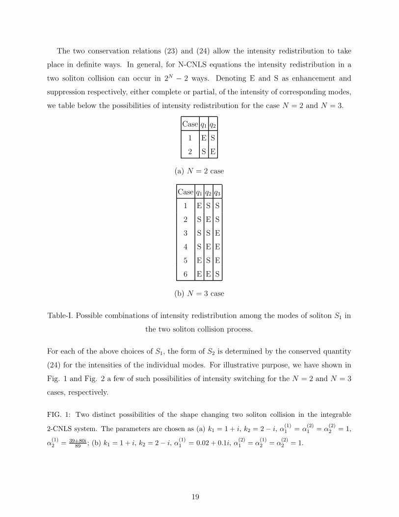
The two conservation relations (23) and (24) allow the intensity redistribution to take

place in definite ways. In general, for N-CNLS equations the intensity redistribution in a

two soliton collision can occur in 2N − 2 ways. Denoting E and S as enhancement and

suppression respectively, either complete or partial, of the intensity of corresponding modes,

we table below the possibilities of intensity redistribution for the case N = 2 and N = 3.

Case q1 q2

1 E S

2 S E

(a) N = 2 case

Case q1 q2 q3

1 E S S

2 S E S

3 S S E

4 S E E

5 E S E

6 E E S

(b) N = 3 case

Table-I. Possible combinations of intensity redistribution among the modes of soliton S1 in

the two soliton collision process.

For each of the above choices of S1, the form of S2 is determined by the conserved quantity

(24) for the intensities of the individual modes. For illustrative purpose, we have shown in

Fig. 1 and Fig. 2 a few of such possibilities of intensity switching for the N = 2 and N = 3

cases, respectively.

FIG. 1: Two distinct possibilities of the shape changing two soliton collision in the integrable

2-CNLS system. The parameters are chosen as (a) k1 = 1 + i, k2 = 2 − i, α(1)1 = α

(2)1 = α

(2)2 = 1,

α(1)2 = 39+80i

89 ; (b) k1 = 1 + i, k2 = 2 − i, α(1)1 = 0.02 + 0.1i, α

(2)1 = α

(1)2 = α

(2)2 = 1.

19

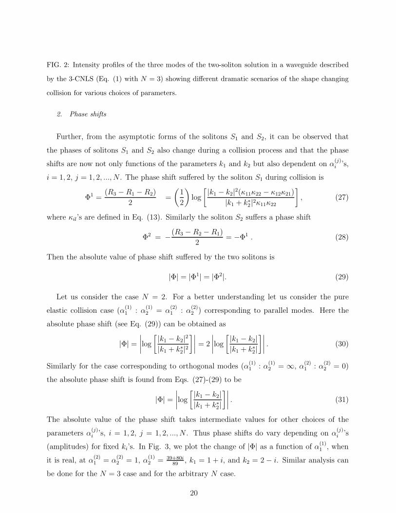
FIG. 2: Intensity profiles of the three modes of the two-soliton solution in a waveguide described

by the 3-CNLS (Eq. (1) with N = 3) showing different dramatic scenarios of the shape changing

collision for various choices of parameters.

2. Phase shifts

Further, from the asymptotic forms of the solitons S1 and S2, it can be observed that

the phases of solitons S1 and S2 also change during a collision process and that the phase

shifts are now not only functions of the parameters k1 and k2 but also dependent on α(j)i ’s,

i = 1, 2, j = 1, 2, ..., N . The phase shift suffered by the soliton S1 during collision is

Φ1 =(R3 − R1 − R2)

2=

(

1

2

)

log

[ |k1 − k2|2(κ11κ22 − κ12κ21)

|k1 + k∗2|2κ11κ22

]

, (27)

where κil’s are defined in Eq. (13). Similarly the soliton S2 suffers a phase shift

Φ2 = −(R3 − R2 − R1)

2= −Φ1 . (28)

Then the absolute value of phase shift suffered by the two solitons is

|Φ| = |Φ1| = |Φ2|. (29)

Let us consider the case N = 2. For a better understanding let us consider the pure

elastic collision case (α(1)1 : α

(1)2 = α

(2)1 : α

(2)2 ) corresponding to parallel modes. Here the

absolute phase shift (see Eq. (29)) can be obtained as

|Φ| =

∣

∣

∣

∣

log

[ |k1 − k2|2|k1 + k∗

2|2]∣

∣

∣

∣

= 2

∣

∣

∣

∣

log

[ |k1 − k2||k1 + k∗

2|

]∣

∣

∣

∣

. (30)

Similarly for the case corresponding to orthogonal modes (α(1)1 : α

(1)2 = ∞, α

(2)1 : α

(2)2 = 0)

the absolute phase shift is found from Eqs. (27)-(29) to be

|Φ| =

∣

∣

∣

∣

log

[ |k1 − k2||k1 + k∗

2|

]∣

∣

∣

∣

. (31)

The absolute value of the phase shift takes intermediate values for other choices of the

parameters α(j)i ’s, i = 1, 2, j = 1, 2, ..., N . Thus phase shifts do vary depending on α

(j)i ’s

(amplitudes) for fixed ki’s. In Fig. 3, we plot the change of |Φ| as a function of α(1)1 , when

it is real, at α(2)1 = α

(2)2 = 1, α

(1)2 = 39+80i

89, k1 = 1 + i, and k2 = 2 − i. Similar analysis can

be done for the N = 3 case and for the arbitrary N case.

20

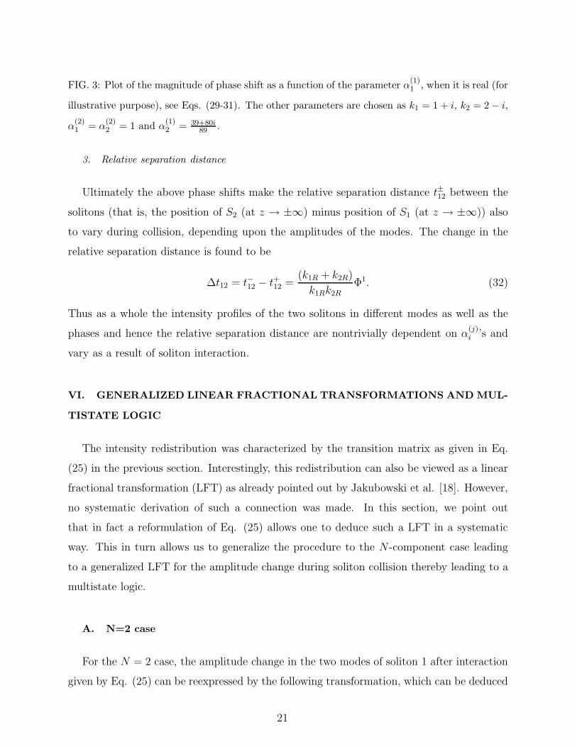
FIG. 3: Plot of the magnitude of phase shift as a function of the parameter α(1)1 , when it is real (for

illustrative purpose), see Eqs. (29-31). The other parameters are chosen as k1 = 1 + i, k2 = 2 − i,

α(2)1 = α

(2)2 = 1 and α

(1)2 = 39+80i

89 .

3. Relative separation distance

Ultimately the above phase shifts make the relative separation distance t±12 between the

solitons (that is, the position of S2 (at z → ±∞) minus position of S1 (at z → ±∞)) also

to vary during collision, depending upon the amplitudes of the modes. The change in the

relative separation distance is found to be

∆t12 = t−12 − t+12 =(k1R + k2R)

k1Rk2R

Φ1. (32)

Thus as a whole the intensity profiles of the two solitons in different modes as well as the

phases and hence the relative separation distance are nontrivially dependent on α(j)i ’s and

vary as a result of soliton interaction.

VI. GENERALIZED LINEAR FRACTIONAL TRANSFORMATIONS AND MUL-

TISTATE LOGIC

The intensity redistribution was characterized by the transition matrix as given in Eq.

(25) in the previous section. Interestingly, this redistribution can also be viewed as a linear

fractional transformation (LFT) as already pointed out by Jakubowski et al. [18]. However,

no systematic derivation of such a connection was made. In this section, we point out

that in fact a reformulation of Eq. (25) allows one to deduce such a LFT in a systematic

way. This in turn allows us to generalize the procedure to the N -component case leading

to a generalized LFT for the amplitude change during soliton collision thereby leading to a

multistate logic.

A. N=2 case

For the N = 2 case, the amplitude change in the two modes of soliton 1 after interaction

given by Eq. (25) can be reexpressed by the following transformation, which can be deduced

21

from comparison of expressions (15b) and (17b):

A1+1 = ΓC11A

1−1 + ΓC12A

1−2 ,

A1+2 = ΓC21A

1−1 + ΓC22A

1−2 . (33a)

Here

Γ = Γ(A1−1 , A1−

2 , A2−1 , A2−

2 )

≡(

a2

a∗2

)

[

1

((α(1)1 α

(1)∗2 + α

(2)1 α

(2)∗2 )(α

(1)2 α

(1)∗2 + α

(2)2 α

(2)∗2 ))

]

[

1

|κ12|2− 1

κ11κ22

]−1/2

,

(33b)

in which a2 is given in Eq. (25c). The forms of Cij’s, i, j = 1, 2, read as

C11 = α(1)2 α

(1)∗2 (k1 − k2) + α

(2)2 α

(2)∗2 (k1 + k∗

2), (33c)

C12 = −α(1)2 α

(2)∗2 (k2 + k∗

2), (33d)

C21 = −α(2)2 α

(1)∗2 (k2 + k∗

2), (33e)

C22 = α(1)2 α

(1)∗2 (k1 + k∗

2) + α(2)2 α

(2)∗2 (k1 − k2). (33f)

Note that the coefficients Cij’s are independent of α(j)1 ’s and so of A1−

1 and A1−2 , that is the

α-parameters of soliton 1. Then from Eqs. (33a) the ratios of the Aj±i ’s, i, j = 1, 2, can be

connected through a linear fractional transformation(LFT). For example, for soliton 1, from

(33a),

ρ1+1,2 =

A1+1

A1+2

=C11ρ

1−1,2 + C12

C21ρ1−1,2 + C22

, (34)

where ρ1−1,2=

A1−1

A1−2

, in which the superscripts represent the underlying soliton and the subscripts

represent the corresponding modes. The quantities ρ1+1,2, ρ1−

1,2, C11, C12, C21, C22, in Eq. (34)

are same as the quantities ρR, ρ1,(

1−h∗

ρ∗L+ ρL

)

, h∗ ρL

ρ∗L, h∗ and

(

(1 − h∗)ρL + 1ρ∗L

)

, respectively,

given by Eq. (9) in Ref. [18] in an adhoc way. Thus the state of S1 before and after

interaction is characterized by ρ1−1,2 and ρ1+

1,2, respectively. It is to be noticed that during

collision ki’s, i = 1, 2, are unaltered. The LFT has been profitably used in Ref. [19] to

construct logic gates, associated with the binary logic ρ = [0, 1]. Similar analysis can be

done for the soliton 2 also.

22

B. N=3 case

Extending the above analysis, straightforwardly one can relate the A1±j ’s, j = 1, 2, 3, for

soliton 1, from Eqs. (19b) and (21b), as

A1+1 = ΓC11A

1−1 + ΓC12A

1−2 + ΓC13A

1−3 , (35a)

A1+2 = ΓC21A

1−1 + ΓC22A

1−2 + ΓC23A

1−3 , (35b)

A1+3 = ΓC31A

1−1 + ΓC32A

1−2 + ΓC33A

1−3 , (35c)

where

Γ = Γ(A1−1 , A1−

2 , A1−3 , A2−

1 , A2−2 , A2−

3 )

≡(

a2

a∗2

)

[

1

((α(1)1 α

(1)∗2 + α

(2)1 α

(2)∗2 + α

(3)1 α

(3)∗2 )(α

(1)2 α

(1)∗2 + α

(2)2 α

(2)∗2 + α

(3)2 α

(3)∗2 ))

]

×[

1

|κ12|2− 1

κ11κ22

]−1/2

, (35d)

in which a2’s are redefined as

a2 = (k2 + k∗1)[(k1 − k2)(α

(1)1 α

(1)∗2 + α

(2)1 α

(2)∗2 + α

(3)1 α

(3)∗2 )]1/2, (35e)

and κil’s can be written from Eq. (13) with N = 3. Note that the form of Γ is a straightfor-

ward extension of the N = 2 case. In the above equations the coefficients Cij’s, i, j = 1, 2, 3,

for the 3-CNLS case can be written down straightforwardly by generalizing the expressions

(33) corresponding to the two-soliton solution of the two component case.

Thus in the two soliton collision process of the N = 3 case, for soliton 1 we obtain the

generalized Mobius transformation,

ρ1+1,3 =

A1+1

A1+3

=C11ρ

1−1,3 + C12ρ

1−2,3 + C13

C31ρ1−1,3 + C32ρ

1−2,3 + C33

, (36a)

ρ1+2,3 =

A1+2

A1+3

=C21ρ

1−1,3 + C22ρ

1−2,3 + C23

C31ρ1−1,3 + C32ρ

1−2,3 + C33

, (36b)

where ρ1−1,3 =

A1−1

A1−3

and ρ1−2,3 =

A1−2

A1−3

. Similar relations can be obtained for the soliton 2 also.

C. Arbitrary N case

Proceeding in a similar fashion one can construct for the soliton S1 a generalized linear

fractional transformation for the N-component case also which relates the ρ vectors before

23

and after collision.

ρ1+i,N =

A1+i

A1+N

=

∑Nj=1 Cijρ

1−j,N

∑Nj=1 CNjρ

1−j,N

, (37a)

with the condition

ρ1−NN = 1. (37b)

Here ρ1−i,N =

A1−i

A1−N

. Similar expression can be obtained for soliton 2 also.

The above generalization paves way not only for writing down the bilinear transformation

but also to identify multistate logic. For example, in the N = 3 case, the following states are

possible: ρ = [ρ1, ρ2] ≡ [(0, 0), (0, 1), (1, 0), (1, 1)], where the logical ‘0’ state can stand for

the complex valued ρ state corresponding to a suppression of the amplitude in that mode,

while the logical ‘1’ state may correspond to enhancement (including no change), which can

be used to perform logical operations, whereas in the N = 2 case we have only the two state

logic, ρ = [0, 1]. This shows that for N > 2, we will get multistate logic and we believe that

such states can be of distinct advantage in computation. This kind of study is in progress.

VII. HIGHER ORDER SOLITON SOLUTIONS AND THEIR INTERACTIONS

Now it is of interest to study the nature of multisoliton collisions making use of the

explicit forms of multisoliton solutions given in Secs. III and IV. Due to the complicated

nature of the above bright soliton expressions, it becomes nontrivial to identify the nature

of the collision process. In his paper [13], Manakov pointed out that in general an N-soliton

collision does not reduce to a pair collision due to the nontrivial dependence of the amplitude

of a particular soliton before interaction on the other soliton parameters. In this section by a

careful asymptotic analysis of the 3-soliton solution (10) of the 2-CNLS equations, which can

be deduced to the N -CNLS case without any difficulty, we explicitly demonstrate that the

collision process indeed can be considered to occur pair-wise and thereby making Manakov’s

statement in proper perspective and clearer. One can carry out a similar analysis for the

four-soliton solution given in Appendix A, generalizing which one can show that in the higher

order solitons of CNLS equations also the collision is pair-wise. Such an analysis also reveals

the many possibilities for energy exchange among the modes of the solitons, including the

exciting possibility of state restoration in higher order soliton solutions, a precursor to the

construction of logic gates.

24

A. Asymptotic analysis of 3-soliton solution of 2-CNLS equations

Considering the explicit three soliton expression (10), without loss of generality, we as-

sume that the quantities k1R, k2R, and k3R are positive and k1I > k2I > k3I (For the equal

sign cases k1I = k2I = k3I , see Sec. IX below). One can carry out similar analysis for other

possibilities of kiI ’s , i = 1, 2, 3, also as discussed below. Then for the above condition the

variables ηiR’s, i = 1, 2, 3, for the three solitons (S1, S2, and S3) take the following values

asymptotically:

(i) η1R ≈ 0, η2R → ±∞, η3R → ±∞, as z → ±∞,

(ii) η2R ≈ 0, η1R → ∓∞, η3R → ±∞, as z → ±∞,

(iii) η3R ≈ 0, η1R → ∓∞, η2R → ∓∞, as z → ±∞.

Defining the various quantities Ri’s, i = 1, 2, ..., 7 , δlj’s, l = 1, 2, ..., 9, j = 1, 2, τmj ’s, and

τm0’s, m = 1, 2, 3, as in Eq. (10) we have the following limiting forms of the three-soliton

solution Eq. (10).

(i)Before Collision (limit z → −∞)

(a) Soliton 1 (η1R ≈ 0, η2R → −∞, η3R → −∞):

q1

q2

≈

A1−1

A1−2

k1Rsech

(

η1R +R1

2

)

eiη1I , (38a)

A1−1

A1−2

=

α(1)1

α(2)1

e−R1

2

(k1 + k∗1)

. (38b)

(b) Soliton 2 (η2R ≈ 0, η1R → ∞, η3R → −∞):

q1

q2

≈

A2−1

A2−2

k2Rsech

(

η2R +R4 − R1

2

)

eiη2I , (39a)

A2−1

A2−2

=

eδ11

eδ12

e−(R1+R4)

2

(k2 + k∗2)

. (39b)

(c) Soliton 3 (η3R ≈ 0, η1R → ∞, η2R → ∞):

q1

q2

≈

A3−1

A3−2

k3Rsech

(

η3R +R7 − R4

2

)

eiη3I , (40a)

A3−1

A3−2

=

eτ11

eτ12

e−(R4+R7)

2

(k3 + k∗3)

. (40b)

25

(ii)After Collision (limit z → +∞)

(a) Soliton 1 (η1R ≈ 0, η2R → ∞, η3R → ∞):

q1

q2

≈

A1+1

A1+2

k1Rsech

(

η1R +R7 − R6

2

)

eiη1I , (41a)

A1+1

A1+2

=

eτ31

eτ32

e−(R6+R7)

2

(k1 + k∗1)

. (41b)

(b) Soliton 2 (η2R ≈ 0, η1R → −∞, η3R → ∞):

q1

q2

≈

A2+1

A2+2

k2Rsech

(

η2R +R6 − R3

2

)

eiη2I , (42a)

A2+1

A2+2

=

eδ61

eδ62

e−(R3+R6)

2

(k2 + k∗2)

. (42b)

(c) Soliton 3 (η3R ≈ 0, η1R → −∞, η2R → −∞):

q3+1

q3+2

≈

A3+1

A3+2

k3Rsech

(

η3R +R3

2

)

eiη3I , (43a)

A3+1

A3+2

=

α(1)3

α(2)3

e−R32

(k3 + k∗3)

. (43b)

B. Transition elements

The above analysis clearly shows that during the three soliton interaction process, there

is a redistribution of intensities among these solitons in the two modes along with amplitude

dependent phase shifts as in the case of the two soliton interaction. The amplitude changes

can be expressed in terms of a transition matrix T lj as

Al+j = T l

jAl−j , j = 1, 2, l = 1, 2, 3. (44)

Explicit forms of the entries of the transition matrix quantifying the amount of intensity

redistribution for the three solitons are as follows.

Soliton 1:

T 11

T 12

=

eτ31

α(1)1

eτ32

α(2)1

e−(R6+R7−R1)

2 . (45a)

26

Soliton 2:

T 21

T 22

=

eδ61−δ11

eδ62−δ12

e−(R3+R6−R1−R4)

2 . (45b)

Soliton 3:

T 31

T 32

=

α(1)3 e−τ11

α(2)3 e−τ12

e−(R3−R4−R7)

2 . (45c)

The various quantities found in the above equations are defined in Eq. (10).

C. Phase shifts

Now let us look into the phase shifts suffered by each of the solitons during collision.

These can be written as

S1 : Φ1 =R7 − R6 − R1

2, (46a)

S2 : Φ2 =R6 − R3 − R4 + R1

2, (46b)

S3 : Φ3 =R3 − R7 + R4

2. (46c)

Here the quantities R1, R2,..., R7 are as given in Eq. (10). Note that each of the phase

shifts Φ1, Φ2, and Φ3 contains a part which depends purely on ki’s, i = 1, 2, 3, and another

part which depends on the amplitude (polarization) parameters α(j)i ’s along with ki’s.

D. Relative separation distances

As a consequence of the above amplitude dependent phase shifts, the relative separation

distances between the solitons t±ij (position of Sj (at z → ± ∞) - position of Si (at z → ±∞), i 6= j, i < j, i, j = 1, 2, 3) also varies as a function of amplitude parameters. The change

in the relative separation distances (∆tij = t−ij − t+ij) can be obtained from the asymptotic

expressions (38-43). They are found to be

∆t12 =Φ1k2R − Φ2k1R

k1Rk2R

, (47a)

∆t13 =Φ1k3R − Φ3k1R

k1Rk3R

, (47b)

∆t23 =Φ2k3R − Φ3k2R

k2Rk3R, (47c)

27

where Φj ’s, j = 1, 2, 3, are defined in Eq. (46) and kjR’s represent the real parts of kj’s.

E. Nature of Collision

Now it is of interest to look into the nature of the collisions in the three soliton interaction

process, that is, whether it is pair-wise or not. This can be answered from the asymptotic

expressions presented in Eqs. (38) to (46). For example, let us consider soliton 1 (S1).

The net change in the amplitudes of the two modes of soliton S1 is given by the transition

amplitudes T 1i , i = 1, 2, that is,

A1+1

A1+2

=

T 11 0

0 T 12

A1−1

A1−2

, (48)

where T 11 and T 1

2 are defined in Eq. (45a). The above form of transition relations is obtained

by expanding (44).

Let us presume first that the collision process is a pair-wise one and then verify this

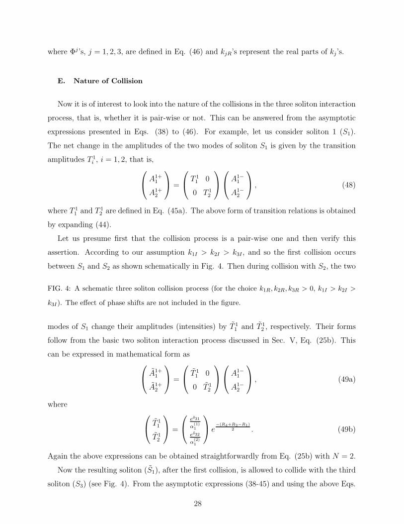
assertion. According to our assumption k1I > k2I > k3I , and so the first collision occurs

between S1 and S2 as shown schematically in Fig. 4. Then during collision with S2, the two

FIG. 4: A schematic three soliton collision process (for the choice k1R, k2R, k3R > 0, k1I > k2I >

k3I). The effect of phase shifts are not included in the figure.

modes of S1 change their amplitudes (intensities) by T 11 and T 1

2 , respectively. Their forms

follow from the basic two soliton interaction process discussed in Sec. V, Eq. (25b). This

can be expressed in mathematical form as

A1+1

A1+2

=

T 11 0

0 T 12

A1−1

A1−2

, (49a)

where

T 11

T 12

=

eδ31

α(1)1

eδ32

α(2)1

e−(R4+R2−R1)

2 . (49b)

Again the above expressions can be obtained straightforwardly from Eq. (25b) with N = 2.

Now the resulting soliton (S1), after the first collision, is allowed to collide with the third

soliton (S3) (see Fig. 4). From the asymptotic expressions (38-45) and using the above Eqs.

28

(49), it can be shown that

A1+1

A1+2

=

T 11 0

0 T 12

A1+1

A1+2

, (50a)

where

T 11

T 12

=

eτ31−δ31

eτ32−δ32

e−(R6+R7−R4−R2)

2 . (50b)

However using Eq. (49) in (50a), we can write

A1+1

A1+2

=

T 11 0

0 T 12

T 11 0

0 T 12

A1−1

A1−2

(51a)

=

T 11 T 1

1 0

0 T 12 T 1

2

A1−1

A1−2

. (51b)

If this is the collision scenario, then the right hand sides of Eq. (48) and Eq. (51b) should

be the same, that is,

T 11 = T 1

1 T 11 , (51c)

T 12 = T 1

2 T 12 . (51d)

This can be easily verified to be true directly from the expressions (45) and (49-50). In

a similar fashion, for the other two solitons also the transition matrix can be shown as a

product of two matrices corresponding to two collisions, respectively.

Now let us look at the phase shifts. It is also of necessary to identify whether the total

phase shift acquired by each soliton during the three soliton collision process is a result

of two consecutive pair-wise collisions or not. In this regard, we again focus our attention

on soliton 1 (S1) first. Let us assume the collision to be pair-wise. Then one can write

the phase shift suffered by S1 during the collision based on the analysis of the two soliton

collision process. Following Eq. (27) (with appropriately changed notations) we can write

the expression for the phase shift suffered by S1 on its collision with S2 as

δ =R4 − R2 − R1

2. (52)

Now the outcoming form of S1 (which is S1) is allowed to interact with S3 (see Fig. 4). The

phase shift during this second collision can again be found from the asymptotic expressions

29

(38-43) as

δ =R7 − R6 − R4 + R2

2. (53)

On the other hand, from the asymptotic expressions (46), the total phase shift suffered by

S1 in a three soliton collision process can be written as

δ =R7 − R6 − R1

2(54)

= δ + δ. (55)

Thus the total phase shift suffered by the soliton 1 is the sum of the phase shifts suffered by

it during pair-wise collisions with soliton 2 and soliton 3, respectively. Similar conclusions

can also be drawn on the phase shifts suffered by the other two solitons as well. Thus the

above analysis on the changes in the amplitudes and phase shifts during the three soliton

collision process establishes the fact that the collisions indeed occur pair-wise.

It may be noted that the above results also imply that the three soliton collision process

is associative and independent of the sequence in which collisions occur, that is whether

the collision occurs in the order S1 → S2 → S3 or S1 → S3 → S2. This property has been

anticipated in the numerical study of Lewis et al. [26], which is now rigorously proved here.

F. Intensity redistributions and shape restoration

The asymptotic analysis not only explains the nature of the collision process, but also

characterizes the collision process. It is clear from the above analysis of the three-soliton

solution that in general there is an intensity redistribution among the three solitons due to

pair-wise interaction in all the two modes along with amplitude dependent phase shifts as

in the two soliton interaction, subject to conservation laws. We have analysed the various

three soliton collision scenarios below.

1. Elastic collision

The standard elastic collision property of solitons results for the special case α(1)1 : α

(1)2 :

α(1)3 = α

(2)1 : α

(2)2 : α

(2)3 . The magnitude of the transition elements |T l

j |, j = 1, 2, and l =

1, 2, 3, becomes one for this choice of parameters and there occurs no intensity redistribution

30

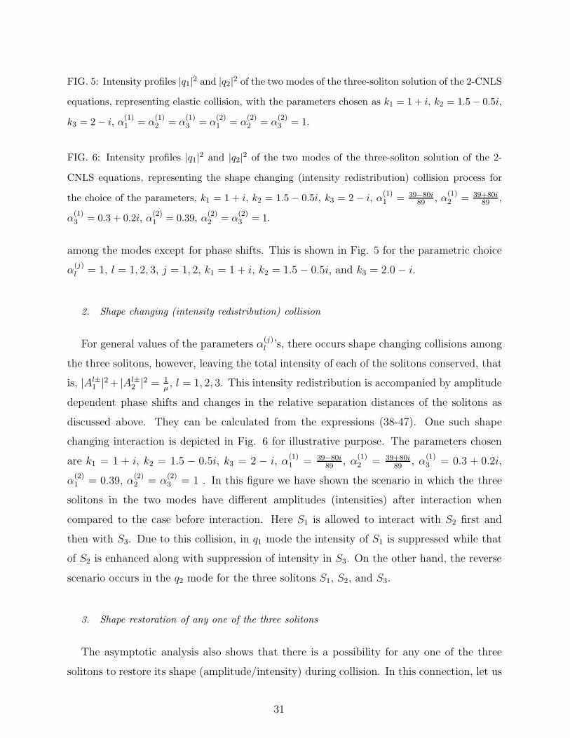
FIG. 5: Intensity profiles |q1|2 and |q2|2 of the two modes of the three-soliton solution of the 2-CNLS

equations, representing elastic collision, with the parameters chosen as k1 = 1 + i, k2 = 1.5 − 0.5i,

k3 = 2 − i, α(1)1 = α

(1)2 = α

(1)3 = α

(2)1 = α

(2)2 = α

(2)3 = 1.

FIG. 6: Intensity profiles |q1|2 and |q2|2 of the two modes of the three-soliton solution of the 2-

CNLS equations, representing the shape changing (intensity redistribution) collision process for

the choice of the parameters, k1 = 1 + i, k2 = 1.5 − 0.5i, k3 = 2 − i, α(1)1 = 39−80i

89 , α(1)2 = 39+80i

89 ,

α(1)3 = 0.3 + 0.2i, α

(2)1 = 0.39, α

(2)2 = α

(2)3 = 1.

among the modes except for phase shifts. This is shown in Fig. 5 for the parametric choice

α(j)l = 1, l = 1, 2, 3, j = 1, 2, k1 = 1 + i, k2 = 1.5 − 0.5i, and k3 = 2.0 − i.

2. Shape changing (intensity redistribution) collision

For general values of the parameters α(j)l ’s, there occurs shape changing collisions among

the three solitons, however, leaving the total intensity of each of the solitons conserved, that

is, |Al±1 |2 + |Al±

2 |2 = 1µ, l = 1, 2, 3. This intensity redistribution is accompanied by amplitude

dependent phase shifts and changes in the relative separation distances of the solitons as

discussed above. They can be calculated from the expressions (38-47). One such shape

changing interaction is depicted in Fig. 6 for illustrative purpose. The parameters chosen

are k1 = 1 + i, k2 = 1.5 − 0.5i, k3 = 2 − i, α(1)1 = 39−80i

89, α

(1)2 = 39+80i

89, α

(1)3 = 0.3 + 0.2i,

α(2)1 = 0.39, α

(2)2 = α

(2)3 = 1 . In this figure we have shown the scenario in which the three

solitons in the two modes have different amplitudes (intensities) after interaction when

compared to the case before interaction. Here S1 is allowed to interact with S2 first and

then with S3. Due to this collision, in q1 mode the intensity of S1 is suppressed while that

of S2 is enhanced along with suppression of intensity in S3. On the other hand, the reverse

scenario occurs in the q2 mode for the three solitons S1, S2, and S3.

3. Shape restoration of any one of the three solitons

The asymptotic analysis also shows that there is a possibility for any one of the three

solitons to restore its shape (amplitude/intensity) during collision. In this connection, let us

31

look into how the shape restoring property of S1 occurs during its collision with the other

two solitons (say S2 and S3). We have already shown that the collision process is a pair-wise

one. Then the three soliton collision process is equivalent to two pair-wise collisions. Let

the first collision be parametrized by the parameters α(1)1 , α

(2)1 , α

(1)2 , α

(2)2 , k1, and k2. Now

we exploit the arbitrariness involved in choosing the parameters α(1)3 and α

(2)3 in the second

collision process in order to make the net transition amplitude of S1 to be unity, leaving the

other two transition amplitudes of S2 and S3 to vary, that is,

T 1j = 1, T 2

j 6= 1, T 3j 6= 1, j = 1, 2. (56)

This condition will make the soliton S1 only to be unaffected at the end of the three soliton

collision process. Then the equations corresponding to this condition are

A1R + A2Rx − A2Iy + A3R(x2 − y2) − 2A3Ixy + A4Rx + A4Iy + A5R(x2 + y2)

+A6R(x3 + xy2) − A6I(x2y + y3) + A7R(x2 − y2)

+2A7Ixy + A8R(x3 + xy2) + A8I(x2y + y3) + A9R(x2 + y2)2 = 0, (57a)

A1I + A2Ry + A2Ix + 2A3Rxy + A3I(x2 − y2) + A4Ix − A4Ry + A5I(x

2 + y2)

+A6I(x3 + xy2) + A6R(x2y + y3) − 2A7Rxy

+A7I(x2 − y2) − A8R(x2y + y3) + A8I(x

3 + xy2) + A9I(x2 + y2)2 = 0, (57b)

B1R + B2Rx − B2Iy + B3R(x2 − y2) − 2B3Ixy + B4Rx + B4Iy + B5R(x2 + y2)

+B6R(x3 + xy2) − B6I(x2y + y3) + B7R(x2 − y2)

+2B7Ixy + B8R(x3 + xy2) + B8I(x2y + y3) + B9R(x2 + y2)2 = 0, (57c)

B1I + B2Ry + B2Ix + 2B3Rxy + B3I(x2 − y2) + B4Ix − B4Ry + B5I(x

2 + y2)

+B6I(x3 + xy2) + B6R(x2y + y3) − 2B7Rxy

+B7I(x2 − y2) − B8R(x2y + y3) + B8I(x

3 + xy2) + B9I(x2 + y2)2 = 0, (57d)

where we have taken

(

α(1)3

α(2)3

)

= x+ iy, the subscripts {lR} and {lI}, l = 1, 2, ..., 9, represent

the real and imaginary parts respectively. The expressions for Ai’s and Bi’s are lengthy but

can be obtained straightforwardly (by making use of (56) and the expressions (45a)) and so

we do not present them here. Solving these overdetermined system of equations for x and

y will give the suitable ratio

(

α(1)3

α(2)3

)

for which the shape restoring property of one of the

solitons S1 only arises in a three soliton collision process.

32

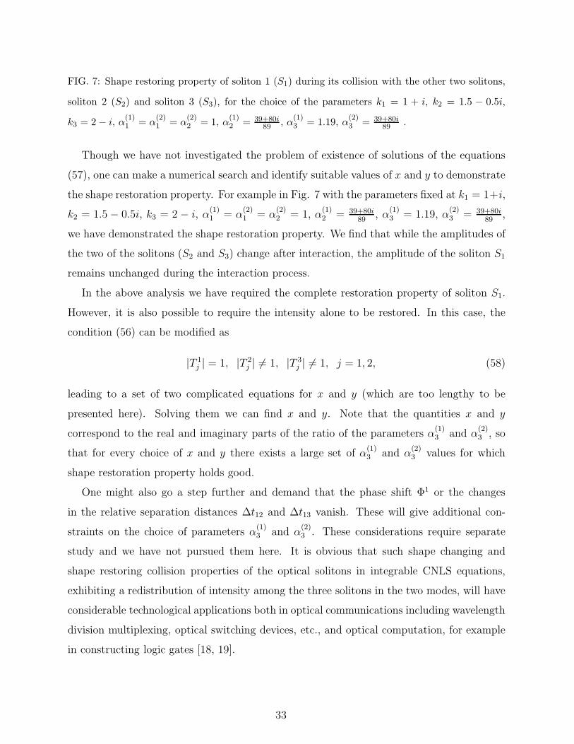
FIG. 7: Shape restoring property of soliton 1 (S1) during its collision with the other two solitons,

soliton 2 (S2) and soliton 3 (S3), for the choice of the parameters k1 = 1 + i, k2 = 1.5 − 0.5i,

k3 = 2 − i, α(1)1 = α

(2)1 = α

(2)2 = 1, α

(1)2 = 39+80i

89 , α(1)3 = 1.19, α

(2)3 = 39+80i

89 .

Though we have not investigated the problem of existence of solutions of the equations

(57), one can make a numerical search and identify suitable values of x and y to demonstrate

the shape restoration property. For example in Fig. 7 with the parameters fixed at k1 = 1+i,

k2 = 1.5 − 0.5i, k3 = 2 − i, α(1)1 = α

(2)1 = α

(2)2 = 1, α

(1)2 = 39+80i

89, α

(1)3 = 1.19, α

(2)3 = 39+80i

89,

we have demonstrated the shape restoration property. We find that while the amplitudes of

the two of the solitons (S2 and S3) change after interaction, the amplitude of the soliton S1

remains unchanged during the interaction process.

In the above analysis we have required the complete restoration property of soliton S1.

However, it is also possible to require the intensity alone to be restored. In this case, the

condition (56) can be modified as

|T 1j | = 1, |T 2

j | 6= 1, |T 3j | 6= 1, j = 1, 2, (58)

leading to a set of two complicated equations for x and y (which are too lengthy to be

presented here). Solving them we can find x and y. Note that the quantities x and y

correspond to the real and imaginary parts of the ratio of the parameters α(1)3 and α

(2)3 , so

that for every choice of x and y there exists a large set of α(1)3 and α

(2)3 values for which

shape restoration property holds good.

One might also go a step further and demand that the phase shift Φ1 or the changes

in the relative separation distances ∆t12 and ∆t13 vanish. These will give additional con-

straints on the choice of parameters α(1)3 and α

(2)3 . These considerations require separate

study and we have not pursued them here. It is obvious that such shape changing and

shape restoring collision properties of the optical solitons in integrable CNLS equations,

exhibiting a redistribution of intensity among the three solitons in the two modes, will have

considerable technological applications both in optical communications including wavelength

division multiplexing, optical switching devices, etc., and optical computation, for example

in constructing logic gates [18, 19].

33

G. Three-soliton solution of multicomponent CNLS equations and shape changing

collisions

The above analysis on the three soliton collision in 2-CNLS equations can be extended

straightforwardly to the 3-soliton solution (14) of N -CNLS equations, with arbitrary N ,

including N = 3. One can identify that shape changing collision occurs here also but

with lot more possibilities for redistribution of intensities in contrast to the 2-CNLS case.

The quantities characterizing the collision process here also are the intensity redistribution,

amplitude dependent phase shifts and relative separation distances between the solitons, as

explained in the 2-CNLS case.

We also note that as the number of components increases from two to some arbitrary N

(N > 2), the different possibilities for redistribution of intensity among them also increase

in a manifold way. The corresponding transition matrix, measuring this redistribution, is

found to be similar to Eqs. (45) with the redefinition of κil’s as given in Eq. (14b) along with

the index j running from 1 to N instead of 1 to 2. The other factors, amplitude dependent

phase shifts and change in relative separation distances, also bear the same form given by

Eqs. (46) and (47), respectively, with this redefinition.

As to the shape restoration property one has to again solve the equations

T 1j = 1, T 2

j 6= 0, T 3j 6= 0, j = 1, 2, 3, ..., N. (59)

Alternatively for intensity restoration the conditions are

|T 1j | = 1, |T 2

j | 6= 0, |T 3j | 6= 0, j = 1, 2, 3, ..., N. (60)

Extending the above analysis, it is clear that, carrying out an asymptotic analysis of 4-

soliton solution given in Appendix A, it is possible to restore the shape of two of the solitons

at the maximum, which can be further generalized to arbitrary N soliton case, in which it

is possible to restore the shape of N − 2 of the solitons. We have checked in this case also

from the asymptotic analysis the soliton interaction is pair-wise and we conjecture that this

should be true for the arbitrary N -soliton case as well.

34

VIII. MULTISOLITON SOLUTIONS AS LOGIC GATES

The state vectors and LFTs introduced in Sec. VI and the shape changing pair-wise

collision nature of bright solitons mentioned in Sec. VII can be profitably used to look at

the multisoliton solutions of CNLS equations as various logic gates. We believe that such

an approach provides an alternative point of view of shape changing soliton collisions to

construct logic gates as discussed in Ref. [19]. The present point of view may have its

own advantage as system initial conditions are chosen suitably to generate specific forms

of multisolitons to represent logic gates may be much easier from a practical point of view,

including replication, compared to constructing them through predetermined independent

soliton collisions. In the following we will demonstrate this idea for the case of the 2-CNLS

as an example.

A. Three soliton solution and state restoration property

The shape restoration of a particular soliton in arbitrary state associated with the three

soliton solution has been discussed in Sec. VII F. Particularly this can be well appreciated

with respect to binary logic states. For example, if we consider the soliton S1 is in 1 state

with the state value ρ1−1,2 = 1, it implies

α(1)1

α(2)1

= 1. (61)

To obtain this we choose, α(1)1 = α

(2)1 = 1. For simplicity we require S2 to be in 0 state

before interaction. From the asymptotic expressions (39), this can be achieved by choosing

the ratioα

(1)2

α(2)2

as

α(1)2

α(2)2

=k1 + k∗

1

2k2 + k∗1 − k1

. (62)

Now in order to restore the state of S1 after two collisions, we have to allow the outcome of

S1 resulting after the first collision, which may be called soliton S ′1, to interact with soliton

S3 having a state inverse to the above 0 state. This state for S3 can be identified from its

asymptotic form before interaction given in Eq. (40). The resulting condition can be shown

35

to be

α(1)3

α(2)3

=n

d, (63a)

n = −(α(1)2 + α

(2)2 )α

(2)∗2 A + κ22(k1 − k∗

1 − 2k3)B + 2α(2)2 α

(2)∗2 C

−α(2)2 (α

(1)∗2 + α

(2)∗2 )D + |α(1)

2 + α(2)2 |2E, (63b)

d = (α(1)2 + α

(2)2 )α

(1)∗2 A − κ22(k1 + k∗

1)B − 2α(2)2 α

(1)∗2 C

−(α(1)∗2 + α

(2)∗2 )α

(2)2 D, (63c)

where

A = (k1 + k∗1)(k3 + k∗

1)(k1 + k∗2), (63d)

B = (k2 + k∗1)(k3 + k∗

2)(k1 + k∗2), (63e)

C = (k2 + k∗1)(k3 + k∗

1)(k1 + k∗2), (63f)

D = (k2 + k∗1)(k3 + k∗

2)(k1 + k∗1), (63g)

E = (k3 + k∗2)(k1 + k∗

1)(k3 + k∗1). (63h)

In the above equation choosing the parameters satisfying conditions (61) and (62) one can

fix

(

α(1)3

α(2)3

)

suitably in order to restore the state of soliton S1. Thus the three soliton solution

given by Eq. (10) having the specific choice of parameters specified by Eqs. (61)-(63)

corresponds to the state restoration of soliton S1.

B. Four-soliton solution and COPY gate

Extending the above procedure, we can now consider the four-soliton solution given in

Appendix A, and identify it as (i) a COPY gate or (ii) a ONE gate or (iii) a NOT gate

studied in Ref. [19] for suitable choices of the arbitrary parameters. As an example, let us

consider copying 1 state of S1 to the output state of soliton S4. This requires the following

steps.

1. We consider the four soliton collision process in which the soliton S1 collides with the

soliton S2 first and then with the soliton S3 and finally with the soliton S4. This

sequence of collision follows from the condition k1I > k2I > k3I > k4I .

2. Consider for convinience S1 to be in the 0 state, the so-called actuator state [19]. This

requiresα

(1)1

α(2)1

= 0, which can be obtained by choosing α(1)1 = 0 and α

(2)1 as arbitrary.

36

3. Assign 1 state to soliton S2 before interaction, for which we need

α(1)2

α(2)2

=k2 − k1

k2 + k∗1

. (64)

4. After its collision with S2 as a result of shape changing collision the outcoming state

of S1 (say S ′1) will be altered.

5. Now let us allow the third soliton in the four soliton solution to interact with S ′1 which

changes the state S ′1 to S ′′

1 .

6. Finally S4 is allowed to interact with S ′′1 . From the asymptotic analysis, we identify

the state of soliton S4 after interaction as

ρ4+1,2 =

α(1)4

α(2)4

. (65)

We impose the condition on this state that this should be in the state of S2 before

interaction. Thus the parameters α(1)4 and α

(2)4 of soliton S4 get fixed depending upon

the input state of S2.

7. The asymptotic analysis of the four soliton solution given in Appendix A results in

following condition for S4 to be in one state after interaction.

T 41 A4−

1

T 42 A4−

2

= 1, (66)

where T 41 and T 4

2 are the transition elements of S4 in the modes q1 and q2 respectively.

Here A4−1 k4R and A4−

2 k4R are the amplitudes of soliton S4 before interaction in the two

modes respectively.

8. If we flip the input state of S2 from 1 to 0 state by suitably choosing the ρ2−1,2’s param-

eters then the condition on soliton S4’s output will become

T 41 A4−

1

T 42 A4−

2

= 0. (67)

9. In the above two Eqs. (66) and (67) only free parameters are α(1)3 and α

(2)3 . In principle,

we can solve these two complex equations to obtain the free complex parameters α(1)3

and α(2)3 . Then for the given choice of parameters the state of the incoming soliton S2

can be copied on to the outgoing soliton S4.

37

Thus a four soliton collision process with the above premise is equivalent to a COPY gate.

Similar procedure can be extended to other gates mentioned above as well. One can extend

this idea further to identify a FANOUT gate from a 5-soliton solution. It appears that one

can pursue the idea ultimately to identify the NAND gate itself as a multisoliton solution

following the construction of Steiglitz in Ref. [19]. Fuller details will be reported elsewhere.

IX. BRIGHT SOLITON SOLUTIONS AND PARTIALLY COHERENT SOLITONS

As mentioned in the introduction, the recent observations by several authors [11, 12, 25]

have shown that the N -CNLS equations (1) can support N -PCSs solutions. In general,

these PCSs are said to be special cases of the so-called multisoliton complexes [2] which are

nonlinear superposition of fundamental bright solitons. It has also been demonstrated that

these PCSs are formed only if the number of components in Eq. (1) is equal to the number

of solitons. Then it is quite natural to look for the 2-PCS, 3-PCS, 4-PCS, etc., as special

cases of the two-soliton solution of the 2-CNLS, three-soliton solution of the 3-CNLS, four-

soliton solution of the 4-CNLS equations etc., respectively, deduced in Secs. III and IV. In

the following, we indeed show that the PCSs reported in Refs.[11, 12, 25] result as special

cases, that is specific choices of some of the arbitrary complex parameters, from the bright

soliton solutions of CNLS equations discussed in Secs. III and IV and thereby showing the

origin of the various interesting properties of the PCS solutions.

A. 2-PCS : A special case of the bright two-soliton solution of 2-CNLS equations

Let us consider stationary limit of the two-soliton solution of the 2-CNLS equations

(Manakov system) given by Eq. (8), that is, knI = 0, for the special choice of the parameters,

α(1)1 = eη10 , α

(2)2 = −eη20 , α

(2)1 = −α

(1)2 = 0, where ηj0’s, j = 1, 2, are now restricted as real

constants. Then Eq. (8) becomes

q1 =

(

eη1 +µ(k1R − k2R)eη1+η2+η∗

2

4k22R(k1R + k2R)

)

/D, (68a)

q2 =

(

−eη2 +µ(k1R − k2R)eη1+η∗

1+η2

4k21R(k1R + k2R)

)

/D, (68b)

38

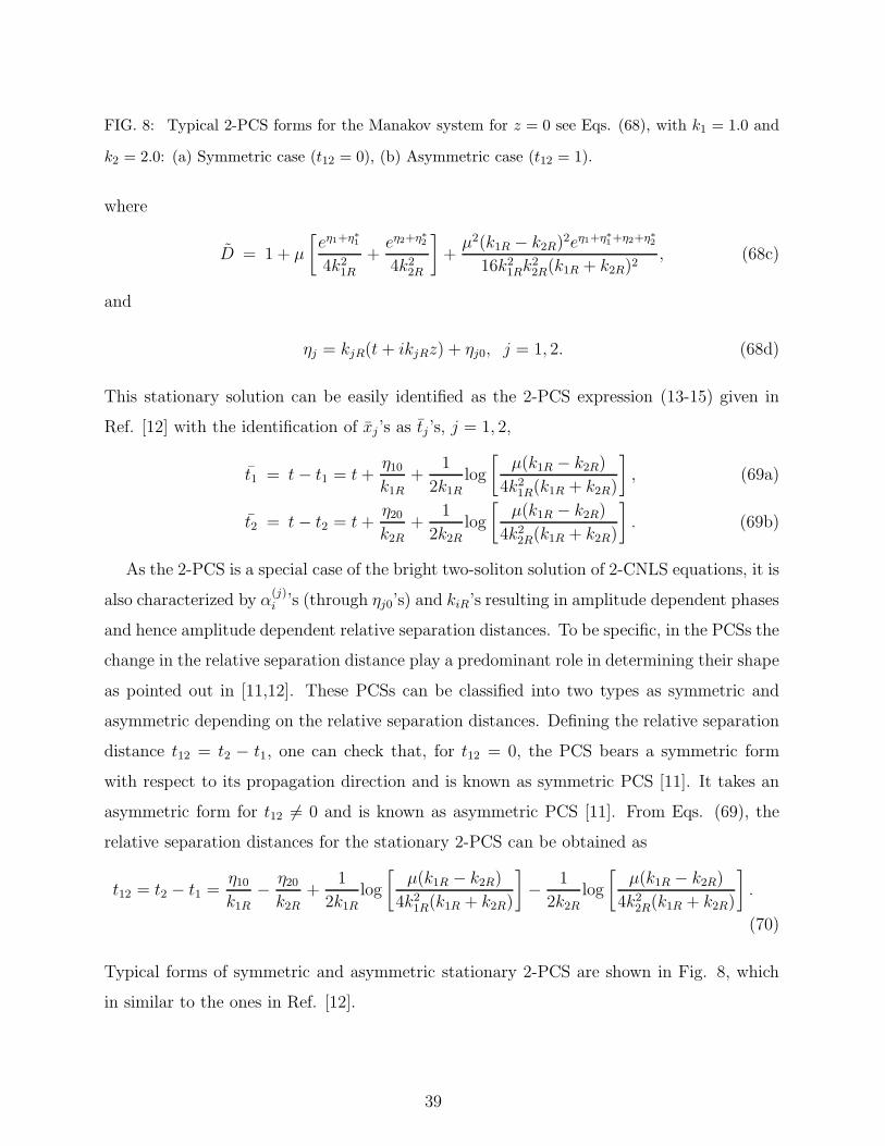
FIG. 8: Typical 2-PCS forms for the Manakov system for z = 0 see Eqs. (68), with k1 = 1.0 and

k2 = 2.0: (a) Symmetric case (t12 = 0), (b) Asymmetric case (t12 = 1).

where

D = 1 + µ

[

eη1+η∗

1

4k21R

+eη2+η∗

2

4k22R

]

+µ2(k1R − k2R)2eη1+η∗

1+η2+η∗

2

16k21Rk2

2R(k1R + k2R)2, (68c)

and

ηj = kjR(t + ikjRz) + ηj0, j = 1, 2. (68d)

This stationary solution can be easily identified as the 2-PCS expression (13-15) given in

Ref. [12] with the identification of xj ’s as tj ’s, j = 1, 2,

t1 = t − t1 = t +η10

k1R

+1

2k1R

log

[

µ(k1R − k2R)

4k21R(k1R + k2R)

]

, (69a)

t2 = t − t2 = t +η20

k2R

+1

2k2R

log

[

µ(k1R − k2R)

4k22R(k1R + k2R)

]

. (69b)

As the 2-PCS is a special case of the bright two-soliton solution of 2-CNLS equations, it is

also characterized by α(j)i ’s (through ηj0’s) and kiR’s resulting in amplitude dependent phases

and hence amplitude dependent relative separation distances. To be specific, in the PCSs the

change in the relative separation distance play a predominant role in determining their shape

as pointed out in [11,12]. These PCSs can be classified into two types as symmetric and

asymmetric depending on the relative separation distances. Defining the relative separation

distance t12 = t2 − t1, one can check that, for t12 = 0, the PCS bears a symmetric form

with respect to its propagation direction and is known as symmetric PCS [11]. It takes an

asymmetric form for t12 6= 0 and is known as asymmetric PCS [11]. From Eqs. (69), the

relative separation distances for the stationary 2-PCS can be obtained as

t12 = t2 − t1 =η10

k1R

− η20

k2R

+1

2k1R

log

[

µ(k1R − k2R)

4k21R(k1R + k2R)

]

− 1

2k2R

log

[

µ(k1R − k2R)

4k22R(k1R + k2R)

]

.

(70)

Typical forms of symmetric and asymmetric stationary 2-PCS are shown in Fig. 8, which

in similar to the ones in Ref. [12].

39

B. 3-PCS: A special case of the bright three-soliton solution of 3-CNLS equations

Since it has been observed that the PCS solutions exist when the number of components

is equal to the number of solitons propagating in the system, we consider next the 3-soliton

solution of the 3-CNLS equations in order to show that the 3-PCS as a special case of the

3-soliton solution. Thus considering the stationary limit knI = 0, n = 1, 2, 3, of the 3-soliton

solution of 3-CNLS equations given by Eq. (14) with N = 3, and making the following

parametric choice

α(1)1 = eη10 , α

(2)2 = −eη20 , α

(3)3 = eη30 , α

(2)1 = α

(3)1 = α

(1)2 = α

(3)2 = α

(1)3 = α

(2)3 = 0, (71)

where ηj0’s, j = 1, 2, 3, are restricted to real parameters, we obtain

q1 =

[

eη1 +µ(k1R − k2R)eη1+η2+η∗

2

4k22R(k1R + k2R)

+µ(k1R − k3R)eη1+η3+η∗

3

4k23R(k1R + k3R)

+µ2(k2R − k1R)(k3R − k1R)(k3R − k2R)2eη3+η∗

3+η2+η∗

2+η1

16k22Rk2

3R(k2R + k1R)(k3R + k1R)(k3R + k2R)2

]

/D1, (72a)

q2 =

[

−eη2 +µ(k1R − k2R)eη1+η∗

1+η2

4k21R(k1R + k2R)

+µ(k3R − k2R)eη3+η∗

3+η2

4k23R(k3R + k2R)

+µ2(k2R − k1R)(k3R − k2R)(k3R − k1R)2eη3+η∗

3+η1+η∗

1+η2

16k21Rk2

3R(k2R + k1R)(k3R + k2R)(k3R + k1R)2

]

/D1, (72b)

q3 =

[

eη3 +µ(k3R − k1R)eη1+η∗

1+η3

4k21R(k1R + k3R)

+µ(k3R − k2R)eη2+η∗

2+η3

4k22R(k3R + k2R)

+µ2(k3R − k1R)(k3R − k2R)(k2R − k1R)2eη2+η∗

2+η1+η∗

1+η3

16k21Rk2

2R(k3R + k1R)(k3R + k2R)(k2R + k1R)2

]

/D1. (72c)

Here,

D1 = 1 + µ

[

eη1+η∗

1

4k21R

+eη2+η∗

2

4k22R

+eη3+η∗

3

4k23R

]

+µ2(k1R − k2R)2eη1+η∗

1+η2+η∗

2

16k21Rk2

2R(k1R + k2R)2

+µ2(k1R − k3R)2eη1+η∗

1+η3+η∗

3

16k21Rk2

3R(k1R + k3R)2+

µ2(k3R − k2R)2eη2+η∗

2+η3+η∗

3

16k22Rk2

3R(k2R + k3R)2

+

[

µ3(k2R − k1R)2(k3R − k1R)2(k3R − k2R)2eη1+η∗

1+η2+η∗

2+η3+η∗

3

64k21Rk2

2Rk23R(k1R + k2R)2(k1R + k3R)2(k2R + k3R)2

]

.

(72d)

The above solution can be easily rewritten as Eq. (16-18) for the 3-PCS case given in Ref.

[12]. As in the case of 2-PCS, here also we identify xj ’s given in Ref. [12] as tj ’s, j = 1, 2, 3,

40

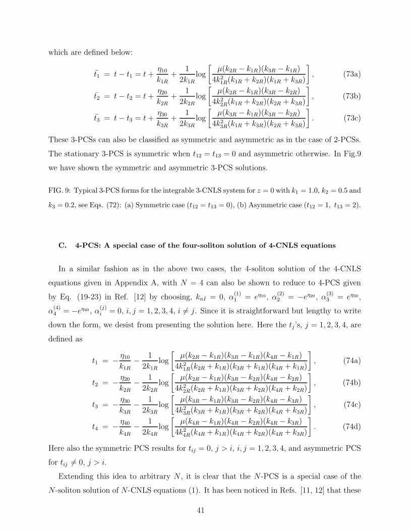
which are defined below:

t1 = t − t1 = t +η10

k1R+

1

2k1Rlog

[

µ(k2R − k1R)(k3R − k1R)

4k21R(k1R + k2R)(k1R + k3R)

]

, (73a)

t2 = t − t2 = t +η20

k2R+

1

2k2Rlog

[

µ(k2R − k1R)(k3R − k2R)

4k22R(k1R + k2R)(k2R + k3R)

]

, (73b)

t3 = t − t3 = t +η30

k3R+

1

2k3Rlog

[

µ(k3R − k1R)(k3R − k2R)

4k23R(k1R + k3R)(k2R + k3R)

]

. (73c)

These 3-PCSs can also be classified as symmetric and asymmetric as in the case of 2-PCSs.

The stationary 3-PCS is symmetric when t12 = t13 = 0 and asymmetric otherwise. In Fig.9

we have shown the symmetric and asymmetric 3-PCS solutions.

FIG. 9: Typical 3-PCS forms for the integrable 3-CNLS system for z = 0 with k1 = 1.0, k2 = 0.5 and

k3 = 0.2, see Eqs. (72): (a) Symmetric case (t12 = t13 = 0), (b) Asymmetric case (t12 = 1, t13 = 2).

C. 4-PCS: A special case of the four-soliton solution of 4-CNLS equations

In a similar fashion as in the above two cases, the 4-soliton solution of the 4-CNLS

equations given in Appendix A, with N = 4 can also be shown to reduce to 4-PCS given

by Eq. (19-23) in Ref. [12] by choosing, knI = 0, α(1)1 = eη10 , α

(2)2 = −eη20 , α

(3)3 = eη30 ,

α(4)4 = −eη40 , α

(j)i = 0, i, j = 1, 2, 3, 4, i 6= j. Since it is straightforward but lengthy to write

down the form, we desist from presenting the solution here. Here the tj’s, j = 1, 2, 3, 4, are

defined as

t1 = − η10

k1R

− 1

2k1R

log

[

µ(k2R − k1R)(k3R − k1R)(k4R − k1R)

4k21R(k2R + k1R)(k3R + k1R)(k4R + k1R)

]

, (74a)

t2 = − η20

k2R

− 1

2k2R

log

[

µ(k2R − k1R)(k3R − k2R)(k4R − k2R)

4k22R(k2R + k1R)(k3R + k2R)(k4R + k2R)

]

, (74b)

t3 = − η30

k3R

− 1

2k3R

log

[

µ(k3R − k1R)(k3R − k2R)(k4R − k3R)

4k23R(k3R + k1R)(k3R + k2R)(k4R + k3R)

]

, (74c)

t4 = − η40

k4R

− 1

2k4R

log

[

µ(k4R − k1R)(k4R − k2R)(k4R − k3R)

4k24R(k4R + k1R)(k4R + k2R)(k4R + k3R)

]

. (74d)

Here also the symmetric PCS results for tij = 0, j > i, i, j = 1, 2, 3, 4, and asymmetric PCS

for tij 6= 0, j > i.

Extending this idea to arbitrary N , it is clear that the N -PCS is a special case of the

N -soliton solution of N -CNLS equations (1). It has been noticed in Refs. [11, 12] that these

41

PCSs are of variable shape. The reason for the variable shape can be traced naturally to

the nontrivial dependence of phases on the complex parameters α(j)i ’s as shown above. Thus

it is clear that any change in the amplitude will affect the phase part of the solitons and

vice-versa. Since we have explicitly shown that N -PCSs are special cases of bright N-soliton

solutions of N -CNLS equations, they possess variable shape as a consequence of the shape

dependence on the α(j)i parameters.

D. Propagation of partially coherent solitons and their collision properties

The intriguing collision properties of the partially coherent solitons reported in Refs. [11,

12] can be well understood by writing down the expression for PCSs with nonvanishing knI ’s,

that is nonstationary special cases of multicomponent higher order bright soliton solutions

discussed in Secs. III and IV. For the nonstationary PCSs we can choose as a special case the

complex parameters α(j)i ’s (i 6= j) to be functions of knI ’s such that they vanish as knI = 0.

As we make these knI 6= 0, then α(j)i ’s (i 6= j) also vary, thereby making the collision scenario

interesting. We can consider both the cases of equal and unequal velocities, which exhibit

similar behaviours.

As a first example, we consider the propagation of the 2-PCS comprising two solitons

with equal velocities (k1I = k2I) in PR media. Its propagation can be studied by choosing

(for illustrative purpose) α(2)1 = k1I and α

(1)2 = (0.25 + 1.02i)k2I as functions of velocities

(kjI , j = 1, 2) such that they vanish when kjI = 0, j = 1, 2. This is shown in Fig. 10 for

the parameters α(1)1 = 2.0 + i, α

(2)2 = 1, k1 = 1.0 + i, and k2 = 2.0 + i. For unequal

velocity case (k1I 6= k2I), the PCS collision is shown in Fig. 11 for the parametric choice

α(1)1 = 1.0, α

(2)1 = k1I , α

(1)2 = −(22+80i

89)k2I , α

(2)2 = −2.0, k1 = 1.0+ i, and k2 = 2.0− i. This

can also be viewed as collision of two 1-PCS which are spread among the two components,

which are travelling with equal but opposite velocities.

FIG. 10: Intensity profiles showing the collision scenario of two 1-PCSs, with equal velocities, at

(a) z = −5 and (b) z = 5, given by special choice of parameters (as given in text) in the 2-soliton

solution of the Manakov system.

Now let us consider the collision of 2-PCS and 1-PCS in PR media. This is equivalent

to the three soliton collision in the 3-CNLS system with specific choice of parameters. We

42

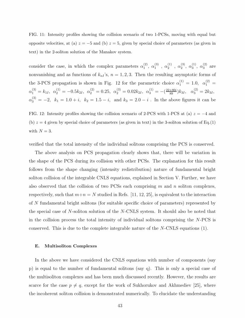
FIG. 11: Intensity profiles showing the collision scenario of two 1-PCSs, moving with equal but

opposite velocities, at (a) z = −5 and (b) z = 5, given by special choice of parameters (as given in

text) in the 2-soliton solution of the Manakov system.

consider the case, in which the complex parameters α(2)1 , α

(3)1 , α

(1)2 , α

(3)2 , α

(1)3 , α

(2)3 are

nonvanishing and as functions of knI ’s, n = 1, 2, 3. Then the resulting asymptotic forms of

the 3-PCS propagation is shown in Fig. 12 for the parametric choice α(1)1 = 1.0, α

(2)1 =

α(3)1 = k1I , α

(1)2 = −0.5k2I , α

(2)2 = 0.25, α

(3)2 = 0.02k2I , α

(1)3 = −(22+80i

89)k3I , α

(2)3 = 2k3I ,

α(3)3 = −2, k1 = 1.0 + i, k2 = 1.5 − i, and k3 = 2.0 − i . In the above figures it can be

FIG. 12: Intensity profiles showing the collision scenario of 2-PCS with 1-PCS at (a) z = −4 and

(b) z = 4 given by special choice of parameters (as given in text) in the 3-soliton solution of Eq.(1)

with N = 3.

verified that the total intensity of the individual solitons comprising the PCS is conserved.

The above analysis on PCS propagation clearly shows that, there will be variation in

the shape of the PCS during its collision with other PCSs. The explanation for this result

follows from the shape changing (intensity redistribution) nature of fundamental bright

soliton collision of the integrable CNLS equations, explained in Section V. Further, we have

also observed that the collision of two PCSs each comprising m and n soliton complexes,

respectively, such that m+n = N studied in Refs. [11, 12, 25], is equivalent to the interaction

of N fundamental bright solitons (for suitable specific choice of parameters) represented by

the special case of N -soliton solution of the N -CNLS system. It should also be noted that

in the collision process the total intensity of individual solitons comprising the N -PCS is

conserved. This is due to the complete integrable nature of the N -CNLS equations (1).

E. Multisoliton Complexes

In the above we have considered the CNLS equations with number of components (say

p) is equal to the number of fundamental solitons (say q). This is only a special case of

the multisoliton complexes and has been much discusssed recently. However, the results are

scarce for the case p 6= q, except for the work of Sukhorukov and Akhmediev [25], where

the incoherent soliton collision is demonstrated numerically. To elucidate the understanding

43

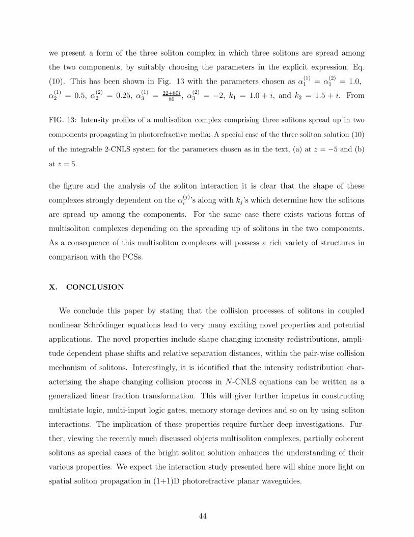
we present a form of the three soliton complex in which three solitons are spread among

the two components, by suitably choosing the parameters in the explicit expression, Eq.

(10). This has been shown in Fig. 13 with the parameters chosen as α(1)1 = α

(2)1 = 1.0,

α(1)2 = 0.5, α

(2)2 = 0.25, α

(1)3 = 22+80i

89, α

(2)3 = −2, k1 = 1.0 + i, and k2 = 1.5 + i. From

FIG. 13: Intensity profiles of a multisoliton complex comprising three solitons spread up in two

components propagating in photorefractive media: A special case of the three soliton solution (10)

of the integrable 2-CNLS system for the parameters chosen as in the text, (a) at z = −5 and (b)

at z = 5.

the figure and the analysis of the soliton interaction it is clear that the shape of these

complexes strongly dependent on the α(j)i ’s along with kj ’s which determine how the solitons

are spread up among the components. For the same case there exists various forms of

multisoliton complexes depending on the spreading up of solitons in the two components.

As a consequence of this multisoliton complexes will possess a rich variety of structures in

comparison with the PCSs.

X. CONCLUSION

We conclude this paper by stating that the collision processes of solitons in coupled

nonlinear Schrodinger equations lead to very many exciting novel properties and potential

applications. The novel properties include shape changing intensity redistributions, ampli-

tude dependent phase shifts and relative separation distances, within the pair-wise collision

mechanism of solitons. Interestingly, it is identified that the intensity redistribution char-

acterising the shape changing collision process in N -CNLS equations can be written as a

generalized linear fraction transformation. This will giver further impetus in constructing

multistate logic, multi-input logic gates, memory storage devices and so on by using soliton

interactions. The implication of these properties require further deep investigations. Fur-

ther, viewing the recently much discussed objects multisoliton complexes, partially coherent

solitons as special cases of the bright soliton solution enhances the understanding of their

various properties. We expect the interaction study presented here will shine more light on

spatial soliton propagation in (1+1)D photorefractive planar waveguides.

44

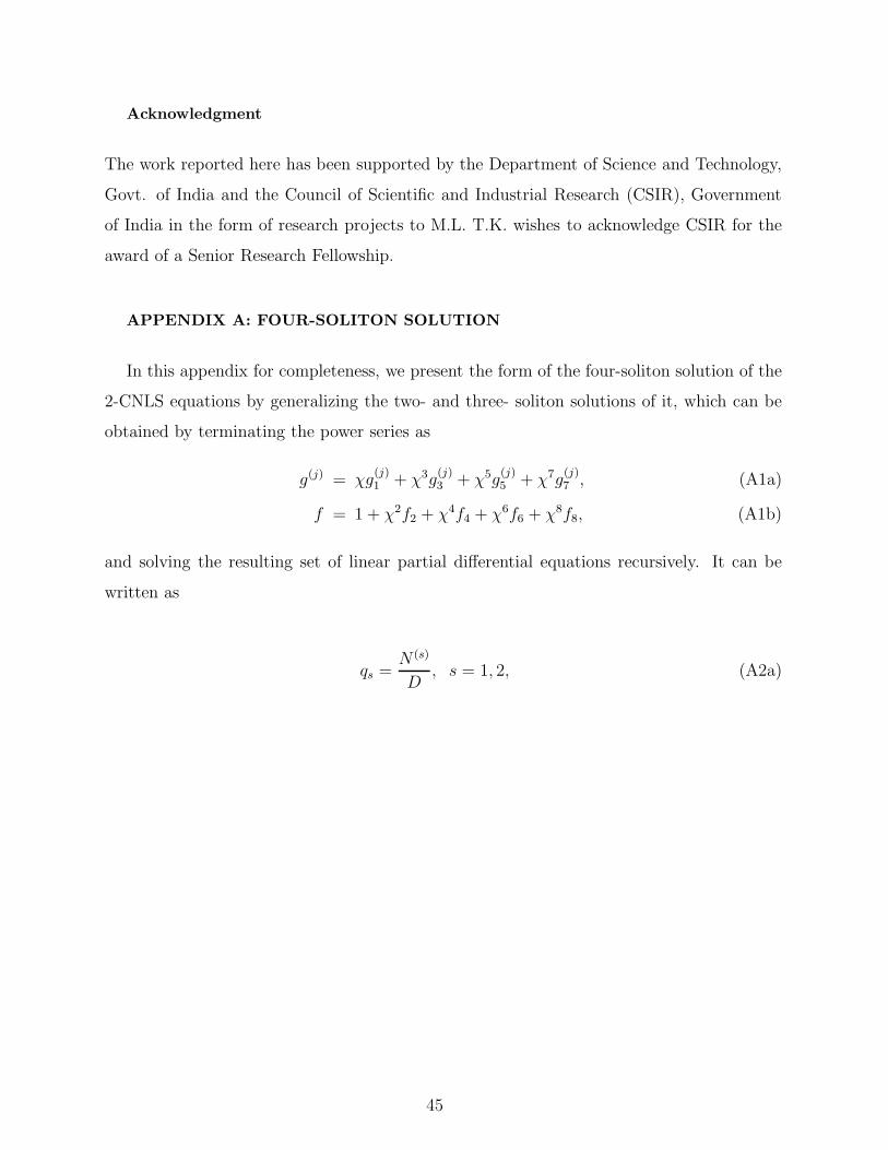
Acknowledgment

The work reported here has been supported by the Department of Science and Technology,

Govt. of India and the Council of Scientific and Industrial Research (CSIR), Government

of India in the form of research projects to M.L. T.K. wishes to acknowledge CSIR for the

award of a Senior Research Fellowship.

APPENDIX A: FOUR-SOLITON SOLUTION

In this appendix for completeness, we present the form of the four-soliton solution of the

2-CNLS equations by generalizing the two- and three- soliton solutions of it, which can be

obtained by terminating the power series as

g(j) = χg(j)1 + χ3g

(j)3 + χ5g

(j)5 + χ7g

(j)7 , (A1a)

f = 1 + χ2f2 + χ4f4 + χ6f6 + χ8f8, (A1b)

and solving the resulting set of linear partial differential equations recursively. It can be

written as

qs =N (s)

D, s = 1, 2, (A2a)

45

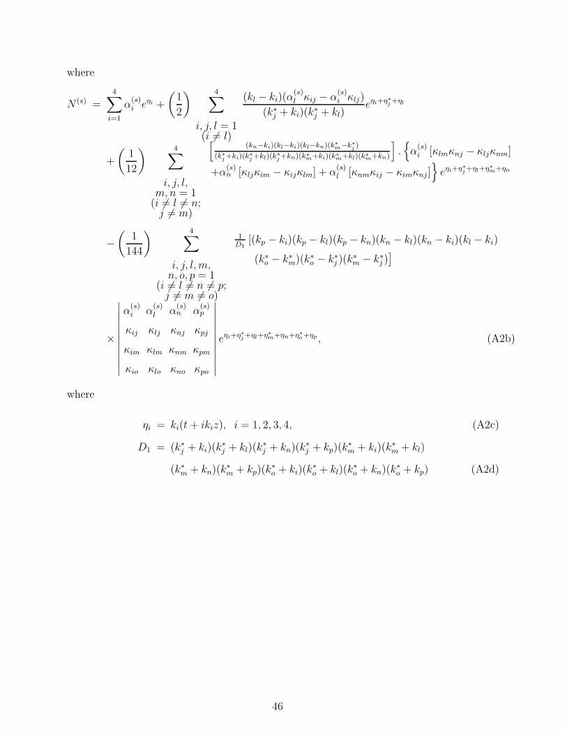
where

N (s) =4

∑

i=1

α(s)i eηi +

(

1

2

) 4∑

i, j, l = 1(i 6= l)

(kl − ki)(α(s)l κij − α

(s)i κlj)

(k∗j + ki)(k

∗j + kl)

eηi+η∗

j +ηl

+

(

1

12

) 4∑

i, j, l,m, n = 1

(i 6= l 6= n;j 6= m)

[

(kn−ki)(kl−ki)(kl−kn)(k∗

m−k∗

j )

(k∗

j +ki)(k∗

j +kl)(k∗

j +kn)(k∗

m+ki)(k∗

m+kl)(k∗

m+kn)

]

.{

α(s)i [κlmκnj − κljκnm]

+α(s)n [κljκim − κijκlm] + α

(s)l [κnmκij − κimκnj ]

}

eηi+η∗

j +ηl+η∗

m+ηn

−(

1

144

) 4∑

i, j, l, m,n, o, p = 1

(i 6= l 6= n 6= p;j 6= m 6= o)

1D1

[(kp − ki)(kp − kl)(kp − kn)(kn − kl)(kn − ki)(kl − ki)

(k∗o − k∗

m)(k∗o − k∗

j )(k∗m − k∗

j )]

×

∣

∣

∣

∣

∣

∣

∣

∣

∣

∣

∣

α(s)i α

(s)l α

(s)n α

(s)p

κij κlj κnj κpj

κim κlm κnm κpm

κio κlo κno κpo

∣

∣

∣

∣

∣

∣

∣

∣

∣

∣

∣

eηi+η∗

j +ηl+η∗

m+ηn+η∗

o+ηp , (A2b)

where

ηi = ki(t + ikiz), i = 1, 2, 3, 4, (A2c)

D1 = (k∗j + ki)(k

∗j + kl)(k

∗j + kn)(k

∗j + kp)(k

∗m + ki)(k

∗m + kl)

(k∗m + kn)(k

∗m + kp)(k

∗o + ki)(k

∗o + kl)(k

∗o + kn)(k∗

o + kp) (A2d)

46

and

D = 1 +4

∑

i,j=1

κij

ki + k∗j

eηi+η∗

j +

(

1

4

) 4∑

i, j, l, m = 1(i 6= l; j 6= m)

(kl − ki)(k∗m − k∗

j )(κijκlm − κimκlj)

(k∗j + ki)(k

∗j + kl)(k∗

m + ki)(k∗m + kl)

eηi+η∗

j +ηl+η∗

m

+

(

1

36

) 4∑

i, j, l,m, n, o = 1(i 6= l 6= n;j 6= m 6= o)

(kn − kl)(kn − ki)(kl − ki)(k∗o − k∗

m)(k∗o − k∗

j )(k∗m − k∗

j )

D2

×

∣

∣

∣

∣

∣

∣

∣

∣

∣

κij κim κio

κlj κlm κlo

κnj κnm κno

∣

∣

∣

∣

∣

∣

∣

∣

∣

eηi+η∗

j +ηl+η∗

m+ηn+η∗

o

+|k1 − k2|2|k2 − k3|2|k3 − k1|2|k4 − k1|2|k2 − k4|2|k3 − k4|2

∏4i=1(ki + k∗

i )|k1 + k∗2|2|k1 + k∗

3|2|k1 + k∗4|2|k2 + k∗

3|2||k2 + k∗4|2|k3 + k∗

4|2∣

∣

∣

∣

∣

∣

∣

∣

∣

∣

∣

κ11 κ12 κ13 κ14

κ21 κ22 κ23 κ24

κ31 κ32 κ33 κ34

κ41 κ42 κ43 κ44

∣

∣

∣

∣

∣

∣

∣

∣

∣

∣

∣

e(η1+η∗

1+η2+η∗

2+η3+η∗

3+η4+η∗

4 ). (A2e)

In the above

D2 = (k∗j + ki)(k

∗j + kl)(k

∗j + kn)(k∗

m + ki)(k∗m + kl)

(k∗m + kn)(k∗

o + ki)(k∗o + kl)(k

∗o + kn), (A2f)

and

κil =µ

(

α(1)i α

(1)∗l + α

(2)i α

(2)∗l

)

(ki + k∗l )

, i, l = 1, 2, 3, 4. (A2g)

[1] G. P. Agrawal, Nonlinear Fiber Optics (Academic Press, New York, 1995).

[2] See for example, several articles in the Focus Issue on “Optical Solitons - Perspectives and

Applications” in Chaos 10, No. 3 (2000).

[3] A. C. Scott, Phys. Scr. 29, 279 (1984).

[4] E. P. Bashkin and A. V. Vagov, Phys. Rev. B 56, 6207 (1997).

47

[5] N. Akhmediev and A. Ankiewicz, Solitons: Nonlinear Pulses and Beams, (Chapman and Hall,

London, 1997).

[6] R. Radhakrishnan, R. Sahadevan, and M. Lakshmanan, Chaos, Solitons and Fractals 5, 2315

(1995).

[7] V. G. Makhan’kov and O. K. Pashaev, Theor. Math. Phys. 53, 979 (1982).

[8] D. N. Christodoulides and M. I. Carvalho, J. Opt. Soc. Am. B 12, 1628 (1995).

[9] D. N. Christodoulides, T. H. Coskun, M. Mitchell, and M. Segev, Phys. Rev. Lett. 78, 646

(1997).

[10] M. Mitchell and M. Segev, Nature (London) 387, 880 (1997).

[11] N. Akhmediev, W. Krolikowski, and A. W. Snyder, Phys. Rev. Lett. 81, 4632 (1998).

[12] A. Ankiewicz, W. Krolikowski, and N. N. Akhmediev, Phys. Rev. E 59, 6079 (1999).

[13] S. V. Manakov, Zh. Eksp. Teor. Fiz. 65, 505 (1973) [Sov. Phys. JETP 38, 248 (1974)].

[14] M. J. Ablowitz and H. Segur, Solitons and the Inverse Scattering Transform, (Siam, Philadel-

phia, 1981).

[15] R. Radhakrishnan, M. Lakshmanan, and J. Hietarinta, Phys. Rev. E 56, 2213 (1997); see

also, M. Lakshmanan, T. Kanna and R. Radhakrishnan, Rep. Math. Phys. 46, 143 (2000).

[16] J. U. Kang, G. I. Stegeman, J. S. Aitchison, and N. Akhmediev, Phys. Rev. Lett. 76, 3699

(1996).

[17] C. Anastassiou et al., Phys. Rev. Lett. 83, 2332 (1999).

[18] M. H. Jakubowski, K. Steiglitz, and R. Squier, Phys. Rev. E 58, 6752 (1998).

[19] K. Steiglitz, Phys. Rev. E 63, 016608 (2000).

[20] T. Kanna and M. Lakshmanan, Phys. Rev. Lett. 86, 5043 (2001).

[21] W. Krolikowski, N. Akhmediev, and B. Luther-Davies, Phys. Rev. E 59, 4654 (1999).

[22] R. Hirota, J. Math. Phys. (N.Y.) 14, 805 (1973).

[23] M. J. Ablowitz, Y. Ohta, and A. D. Trubatch, Phys. Lett. A 253, 287 (1999).

[24] K. W. Chow and D. W. C. Lai, J. Phys. Soc. Jp. 67, 3721 (1998).

[25] A. A. Sukhorukov and N. N. Akhmediev, Phys. Rev. Lett. 83, 4736 (1999).

[26] D. P. Lewis, K. Steiglitz, M. H. Jakubowski, and R. Squier, State Change Operations for

Manakov Soliton Collisions are Associative (but not Commutative) (unpublished).

48

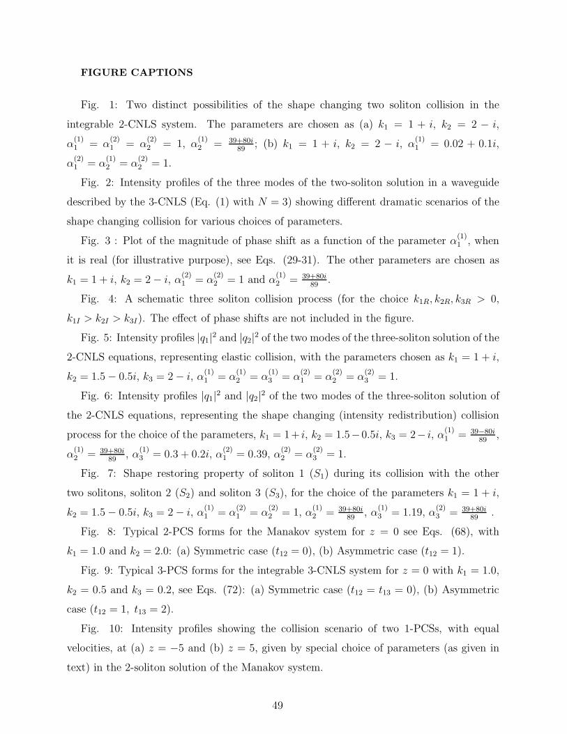
FIGURE CAPTIONS

Fig. 1: Two distinct possibilities of the shape changing two soliton collision in the

integrable 2-CNLS system. The parameters are chosen as (a) k1 = 1 + i, k2 = 2 − i,

α(1)1 = α

(2)1 = α

(2)2 = 1, α

(1)2 = 39+80i

89; (b) k1 = 1 + i, k2 = 2 − i, α

(1)1 = 0.02 + 0.1i,

α(2)1 = α

(1)2 = α

(2)2 = 1.

Fig. 2: Intensity profiles of the three modes of the two-soliton solution in a waveguide

described by the 3-CNLS (Eq. (1) with N = 3) showing different dramatic scenarios of the

shape changing collision for various choices of parameters.

Fig. 3 : Plot of the magnitude of phase shift as a function of the parameter α(1)1 , when

it is real (for illustrative purpose), see Eqs. (29-31). The other parameters are chosen as

k1 = 1 + i, k2 = 2 − i, α(2)1 = α

(2)2 = 1 and α

(1)2 = 39+80i

89.

Fig. 4: A schematic three soliton collision process (for the choice k1R, k2R, k3R > 0,

k1I > k2I > k3I). The effect of phase shifts are not included in the figure.

Fig. 5: Intensity profiles |q1|2 and |q2|2 of the two modes of the three-soliton solution of the

2-CNLS equations, representing elastic collision, with the parameters chosen as k1 = 1 + i,

k2 = 1.5 − 0.5i, k3 = 2 − i, α(1)1 = α

(1)2 = α

(1)3 = α

(2)1 = α

(2)2 = α

(2)3 = 1.

Fig. 6: Intensity profiles |q1|2 and |q2|2 of the two modes of the three-soliton solution of

the 2-CNLS equations, representing the shape changing (intensity redistribution) collision

process for the choice of the parameters, k1 = 1+ i, k2 = 1.5−0.5i, k3 = 2− i, α(1)1 = 39−80i

89,

α(1)2 = 39+80i

89, α

(1)3 = 0.3 + 0.2i, α

(2)1 = 0.39, α

(2)2 = α

(2)3 = 1.

Fig. 7: Shape restoring property of soliton 1 (S1) during its collision with the other

two solitons, soliton 2 (S2) and soliton 3 (S3), for the choice of the parameters k1 = 1 + i,

k2 = 1.5 − 0.5i, k3 = 2 − i, α(1)1 = α

(2)1 = α

(2)2 = 1, α

(1)2 = 39+80i

89, α

(1)3 = 1.19, α

(2)3 = 39+80i

89.

Fig. 8: Typical 2-PCS forms for the Manakov system for z = 0 see Eqs. (68), with

k1 = 1.0 and k2 = 2.0: (a) Symmetric case (t12 = 0), (b) Asymmetric case (t12 = 1).

Fig. 9: Typical 3-PCS forms for the integrable 3-CNLS system for z = 0 with k1 = 1.0,

k2 = 0.5 and k3 = 0.2, see Eqs. (72): (a) Symmetric case (t12 = t13 = 0), (b) Asymmetric

case (t12 = 1, t13 = 2).

Fig. 10: Intensity profiles showing the collision scenario of two 1-PCSs, with equal

velocities, at (a) z = −5 and (b) z = 5, given by special choice of parameters (as given in

text) in the 2-soliton solution of the Manakov system.

49

Fig. 11: Intensity profiles showing the collision scenario of two 1-PCSs, moving with equal

but opposite velocities, at (a) z = −5 and (b) z = 5, given by special choice of parameters

(as given in text) in the 2-soliton solution of the Manakov system.

Fig. 12: Intensity profiles showing the collision scenario of 2-PCS with 1-PCS at (a)

z = −4 and (b) z = 4 given by special choice of parameters (as given in text) in the

3-soliton solution of Eq.(1) with N = 3.

Fig. 13: Intensity profiles of a multisoliton complex comprising three solitons spread up

in two components propagating in photorefractive media: A special case of the three soliton

solution (10) of the integrable 2-CNLS system for the parameters chosen as in the text, (a)

at z = −5 and (b) at z = 5.

50

This figure "fig1.jpg" is available in "jpg" format from:

http://arxiv.org/ps/nlin/0303025v1

This figure "fig2.jpg" is available in "jpg" format from:

http://arxiv.org/ps/nlin/0303025v1

This figure "fig3.jpg" is available in "jpg" format from:

http://arxiv.org/ps/nlin/0303025v1

This figure "fig4.jpg" is available in "jpg" format from:

http://arxiv.org/ps/nlin/0303025v1

This figure "fig5.jpg" is available in "jpg" format from:

http://arxiv.org/ps/nlin/0303025v1

This figure "fig6.jpg" is available in "jpg" format from:

http://arxiv.org/ps/nlin/0303025v1

This figure "fig7.jpg" is available in "jpg" format from:

http://arxiv.org/ps/nlin/0303025v1

This figure "fig8.jpg" is available in "jpg" format from:

http://arxiv.org/ps/nlin/0303025v1

This figure "fig9.jpg" is available in "jpg" format from:

http://arxiv.org/ps/nlin/0303025v1

This figure "fig10.jpg" is available in "jpg" format from:

http://arxiv.org/ps/nlin/0303025v1

This figure "fig11.jpg" is available in "jpg" format from:

http://arxiv.org/ps/nlin/0303025v1

This figure "fig12.jpg" is available in "jpg" format from:

http://arxiv.org/ps/nlin/0303025v1

This figure "fig13.jpg" is available in "jpg" format from:

http://arxiv.org/ps/nlin/0303025v1