arX

iv:m

ath-

ph/0

6070

30v2

15

Aug

200

6

February 7, 2008

Transition to Chaos in Discrete NonlinearSchrodinger Equation with Long-Range Interaction

Nickolay Korabela,1, George M. Zaslavskya,b

a Courant Institute of Mathematical Sciences, New York University

251 Mercer Street, New York, NY 10012, USA,b Department of Physics, New York University,

2-4 Washington Place, New York, NY 10003, USA

Abstract

Discrete nonlinear Schrodinger equation (DNLS) describes a chain of oscillatorswith nearest neighbor interactions and a specific nonlinear term. We consider itsmodification with long-range interaction through a potential proportional to 1/l1+α

with fractional α < 2 and l as a distance between oscillators. This model is calledαDNLS. It exhibits competition between the nonlinearity and a level of correlationbetween interacting far-distanced oscillators, that is defined by the value of α. Weconsider transition to chaos in this system as a function of α and nonlinearity. Itis shown that decreasing of α with respect to nonlinearity stabilize the system.Connection of the model to the fractional genezalization of the NLS (called FNLS)in the long-wave approximation is also discussed and some of the results obtainedfor αDNLS can be correspondingly extended to the FNLS.

PACS: 45.05.+x; 45.50.-j; 45.10.Hj

Keywords: Long-range interaction, Discrete NLS, Fractional equations, Spatio-temporal chaos

1 Introduction

Nonlinear Schrodinger equation (NLS) is a paradigmatic equation that describes a slowly varyingenveloping process in the nonlinear dispersive media. Applications of the NLS has been foundin almost all important areas of physics: nonlinear optics, plasma physics, hydrodynamics,condenced matter physics, biology and others. The literature on NLS is extensive and thereviews [1, 2, 3, 4, 5, 6] can provide a strong impression on the importance of the subject. TheNLS per se is an integrable system while its different types of perturbations, more related to thepractical needs, include a broad spectrum of solutions from solitons and breathers to chaos andspatio-temporal turbulence.

1Corresponding author. Tel.: +1 212 998 3260; fax: +1 212 995 4640.E-mail address: korabel@cims.nyu.edu.

1

Between different types of perturbations one can single out two the most interesting classes:external time-space dependent perturbation, and discretization of the NLS presented by a kindof space-difference equation, called discrete NLS (DNLS). It was shown in a set of publica-tions (see [7, 8, 9] and references therein) that specific hyperbolic structure of the NLS phasespace leads to the transition from a soliton type dynamics to different kind of chaos, includingspatio-temporal turbulence, under even small perturbation. The fact that discretization induceschaos is fairly well known and, particularly, for the DNLS it was studied in [10, 11, 12, 13, 14]and [15, 16]. Destruction of solitons, breathers, and wave trains is similar to what occurs fromexternal perturbations. A general physical mechanism of the onset of chaos induced by a dis-cretization is known: transition from a differential equation to the difference one is equivalentto the appearance of a high frequency (in time or in space) periodic perturbation [17].

One can also consider DNLS as a separate problem that describes a chain of coupled many-particles (oscillators) with local or nonlocal interaction. Such a system presents a specific interestfor studying transition to chaos, turbulence, and statistical equilibrium in many-body problem.A new attraction at that point is the long-range interaction (LRI) that was introduced in anexponential Kac-Baker form in [18, 19] and later in a power Lennard-Jones form in [20]. Inanother version of the latter case the interaction between oscillators located at the positions(n,m), n 6= m, is proportional to 1/|n−m|1+α. The corresponding DNLS will be called αDNLS.Studying of such systems has multiple interest: transition to chaos and turbulence in the presenceof LRI [21, 22], sinchronization in systems with many particles [23], controling chaos [24], anddifferent manipulations with physical objects in optics [1, 25] and condenced matter [26, 27].All these physical features, being described by αDNLS, are functions of α.

For the number of particles N = 4 the DNLS equation can be solved exactly. For N > 4the DNLS is not integrable and chaotic solutions are possible. It was shown in [13, 15, 28,29, 30, 31] that there are two main mechanisms responsible for chaotization of the DNLS. Oneof the mechanisms prevails for symmetric initial conditions and another for asymmetric ones.For symmetric initial conditions chaos was shown to emerge from the proximity to homoclinicorbits. For asymmetric initial conditions this mechanims do not play significant role, instead,perturbations induced by discretization and round-off errors cause random flipping of wave’sdirection of motion.

The primary goal of this paper is to study the transition to chaos in αDNLS depending ona parameter 0 < α < 2 that is responsible for the appearance of a power-like tail in solution,i.e. for the delocalization of modes. Parameter α has a simple physical meaning: it describes alevel of collective coupling of particles. Particularly, for α = ∞ we have only nearest neighborinteraction and for α = −1 we have mean field type model.

Recenly, different properties of the nonlocal DNLS were studied in [32, 33, 34, 35]. It wasfound that some properties of solutions depend on the interaction exponent α in the LRI case oron the exponent β for the Kac-Baker interactions. Namely, for the power-law interaction it wasshown that for α less than some critical value αcr, there is an interval of bistability where threeposible stationary states exist at each value of some excitation number M that characterizea level of nonlinearity. The first type of solution is a continuum-like mode, the second is anintrinsically localized breathing state and the third one is stationary itermediate state. Thelong-distance behavior of the intrinsically localized states depends on α. For α > 2 their tailsare exponential, while for 0 < α < 2 the tails are algebraic. By changing an interaction constantJ , a stable solution may become unstable. A small symmetric force applied to the system canalso trigger transigions from one type of stable solutions to another [33]. The continuum limit

2

of this model was shown to be a nonlocal NLS equation [32]. Another version of the nonlocal(integro-differential) NLS equation was proposed in [36]. Unlike the usual NLS equation, thisnonlocal NLS equation has stationary solutions only in a finite interval of excitation numbers[0,Mmax].

In a similar way, as dynamics of a chain of coupled oscillators can be reduced to the waveequation in the long wave-length limit k → 0, the chain of αDNLS can be reduced to thefractional generalization of NLS equation or Ginzburg-Landau equation (FGL) [37, 38, 39, 23,40, 41]. It was shown in [39, 23] that mapping of the αDNLS equation to fractional NLS (FNLS),or similarly to FGL, can be realized by some transform operator. In all fractional equations ofthis type second coordinate derivative is replaced by the fractional Riesz derivative [42] of orderα. The corresponding comparison of solutions of discrete chain of oscillators with the sine-potential and fractional generalization of the sine-Gordon equation was perfomed in [27, 43].The latter results of [43] confirm a path to the dual features of the systems with LRI of order αand the systems described by a corresponding equation with fractional derivative [39, 23].

In this paper we provide a detailed study of the transition to chaos in αDNLS dependingon the parameter 0 < α < 2. It is well known that fractional values of α appears in numerouscomplex systems such as spin-interacting systems [44], adatoms [26], colloids [45], chemicalsurfaces [46], quantum field theory [47, 48, 49], etc. In correspondence to the results [39, 23, 40],the obtained properties of the αDNLS can be extended to the FNLS. It will be shown thatonset of chaos follows as a result of competition between the nonlinearity level and the level ofcoherency of the chain of oscillators defined by the value of α.

2 Basic equations

The continuous Nonlinear Schrodinger (NLS) equation defined on the finite interval [−L/2, L/2]with the periodic boundary conditions ψ(x+ L, t) = ψ(x, t) can be written as

idψ

dt+ γ|ψ|2ψ +

∂2ψ

∂x2= 0, (1)

where γ is a constant (γ = 1 corresponds to the focusing nonlinearity). In turn, the discretenonlinear Schrodinger equation (DNLS) which describes a lattice of N anharmonic oscillatorswith nearest-neighbors interaction is defined as

idψn

dt+ γ|ψn|2ψn + ǫ (ψn+1 − 2ψn + ψn−1) = 0, (n = 1, ..., N), (2)

where ψn+N = ψn, ∀n is the periodic boundary condition. The quantity ψn = ψn(t) is thecomplex amplitude of the oscillator at site n. With ǫ = 1/(∆x)2, Eq. (2) is seen as a standardfinite difference approximation to Eq. (1). Here ∆x = L/N is a distance between oscillators.

The Hamiltonian, H, and the excitation number (or norm), M ,

H =

N∑

n=1

(

ǫ|ψn+1 − ψn|2 −γ

2|ψn|4

)

, M =

N∑

n=1

|ψn|2, (3)

are the conserved quantities.

3

The model which we study in the following is described by the Hamiltonian

H =1

2

N∑

n=1

N∑

m=1m6=n

Jn−m|ψm − ψn|2 − γ|ψn|4

, (4)

with the periodic boundary conditions: ψn+N = ψn. The coupling function is defined by

Jn−m =J

|n−m|1+α, (n 6= m), (5)

where J is a coupling constant and α is an exponent which, depending on the physical situation,can be integer or fractional. The standard nearest-neighbor DNLS equation is recovered in thelimit α→∞. From the Hamiltonian Eq. (4) one obtain the equation of motion

idψn

dt= ∂H/∂ψ∗

n, (6)

idψn

dt+ γ|ψn|2ψn +

N∑

m=1m6=n

Jn−m(ψn − ψm) = 0, (n = 1, ..., N). (7)

Consider the infinite chain of equidistant oscillators (N → ∞ in Eq. (7)). The Fouriertransform of ψn is given as

ψn(k, t) =∞∑

n=−∞

ψn(t) exp(−ikxn) ≡ F∆{ψn(t)}, (8)

where xn = n∆x is a coordinate of the n-th oscillator, and ∆x = 2π/K is a distance betweenoscillators. Here we have treated k as a continuous variable. The inverse transform is definedas

ψn(t) =1

K

∫ +K/2

−K/2dk ψn(k, t) exp(ikxn) ≡ F−1

∆ {ψn(t)}, (9)

Transition to the continuous limit ∆x→ 0 (K →∞) can be obtained by transforming ψn(t) =ψ(n∆x, t) = ψ(xn, t)→ ψ(x, t). Then, changing sums into integrals, Eqs. (8), (9) become

ψ(k, t) =

∫ +∞

−∞dx e−ikxψ(x, t) ≡ F{ψ(x, t)}, (10)

ψ(x, t) =1

2π

∫ +∞

−∞dk eikxψ(k, t) ≡ F−1{ψ(k, t)}, (11)

whereψ(k, t) = Lψ(k, t), ψ(x, t) = Lψn(t) = Lψ(xn, t), (12)

and L denotes the limit ∆x→ 0. Operation T = F−1L F∆ can be called a transform operator(or transform map), since it performs a tranfrormation of a discrete model of coupled oscillatorsto the continuous media. For 0 < α < 2 application of T leads to the fractional NLS. For more

4

details, definitions and applications of the transform operator to different systems see [23, 40, 43].In a brief form this approximation is as follows [39, 23].

First we perform the Fourier tranformation of Eq. (7) for infinite chain of oscillators (N →∞)

i∂ψ(k, t)

∂t+ γ F∆{|ψn|2ψn}+ J (Jα(k)− Jα(0)) ψ(k, t) = 0, (13)

where

Jα(k) =+∞∑

n=−∞n 6=0

e−ikn∆x

|n|1+α=

+∞∑

n=1

e−ikn∆x + eikn∆x

n1+α= Li1+α(eik∆x) + Li1+α(e−ik∆x), (14)

and Li1+α(z) is a polylogarithm function [50] with series representation

Jα(k) = aα |∆x|α |k|α + 2

∞∑

n=0

ζ(1 + α− 2n)

(2n)!(∆x)2n(−k2)n, |k| < 1, α 6= 0, 1, 2, 3... . (15)

Here Jα(0) = 2ζ(1 + α), ζ is the Riemann zeta-function and

aα = 2 Γ(−α) cos(πα

2

)

. (16)

For α = 2, Jα(k) reduces to the Clausen function Cl2(k) [51].Substitution of Eqs. (15) and (16) into (13) gives

i∂ψ(k, t)

∂t+ J ψ(k, t)

(

aα|∆x|α |k|α + 2∞∑

n=0

ζ(α+ 1− 2n)

(2n)!(∆x)2n(−k2)n − Jα(0)

)

+ (17)

+γ F∆{|ψn|2ψn} = 0.

Note that Jα(0) exactly cancels the constant which is the first term of the sum in Eq. (17). Inthe limit k → 0 Eq. (17) yields

i∂ψ(k, t)

∂t+ J Tα,∆(k) ψ(k, t) + γ F∆{|ψn|2ψn} = 0, (18)

where J = J |∆x|min{α,2} and

Tα,∆(k) =

{

aα|k|α − |∆x|2−αζ(α− 1)k2, 0 < α < 2, (α 6= 1)

|∆x|α−2aα|k|α − ζ(α− 1)k2, 2 < α < 4, (α 6= 3).(19)

For 0 < α < 2 the operator Tα,∆(k) is defined up to O(k2) and for 2 < α < 4 up to O(|k|α).Eq. (19) has a crossover scale for

k0 = |aα/ζ(α− 1)|1/(2−α)|∆x|−1. (20)

From Eq. (20) it follows that Tα,∆(k) ∼ k2 for α > 2, k ≪ k0 and nontrivial expression

Tα,∆(k) ∼ |k|α appears only for α < 2, k ≪ k0. This crossover was considered also in [39, 23].

5

Performing the transition to the limit k ≪ k0 (or more precisely k∆x ≪ k0∆x) and applyingthe inverse Fourier transform to (18), we obtain

i∂

∂tψ(x, t) + J Tα(x) ψ(x, t) + γ |ψ(x, t)|2ψ(x, t) = 0 α 6= 0, 1, 2, ..., (21)

where

Tα(x) = F−1{Tα(k)} =

{

−aα∂α

∂|x|α , 0 < α < 2, (α 6= 1)

ζ(α− 1) ∂2

∂x2 , α > 2, (α 6= 2, 3, 4, ...);(22)

Tα(k) =

{

aα|k|α, 0 < α < 2, (α 6= 1)

−ζ(α− 1) k2, α > 2, (α 6= 2, 3, 4, ...).

Here, we have used the connection between the Riesz fractional derivative and its Fourier trans-form [42]:

|k|α ←→ − ∂α

∂|x|α , k2 ←→ − ∂2

∂x2. (23)

Properties of the Riesz fractioanl derivative can be found in [42, 52, 53, 54].In the following section we will consider simulations of the finite chain of oscillators on a

finite interval (−L/2, L/2) (n = 1, ..., N , where N is even) described by the Hamiltonian

H =

N∑

n=1

J

N/2−1∑

l=1

|ψn+l − ψn|2l1+α

− γ

2|ψn|4

(24)

and equation of motion

idψn

dt+ γ|ψn|2ψn + J

N/2−1∑

l=1

ψn+l − 2ψn + ψn−l

l1+α= 0, (n = 1, ..., N). (25)

The form of the Hamiltonian and the equation of motion account for the periodic boundaryconditions ψn+N = ψn. To avoid double counting of interactions we introduce a cutoff for theinteraction range at N/2 − 1.

All initial conditions and parameters are choosen to make it possible to use the transformoperator T . This means that for not too large time the obtained results can be also applied tothe FDNLS equation (21)

i∂

∂tψ(x, t) −G ∂αψ(x, t)

∂|x|α ψ(x, t) + γ |ψ(x, t)|2ψ(x, t) = 0, 0 < α < 2, α 6= 1, (26)

G = 2 J |∆x|α Γ(−α) cos(πα/2). (27)

It is also worthwile to mention that for α→ 2 we satisfy the conditions of the continuous limitapproach since k0 → ∞, that means the corresponding results should be close to the solutionof NLS. Thus, considering α far from α = 2, one can compare the solutions of αDNLS withthe solutions of DNLS with the nearest neighbor interaction. Such results provide a role of thelong-range interaction for the chain dynamics.

6

3 Numerical results

In this section numerical results obtained from solutions of the equations of motion Eq. (25) onthe finite interval (−L/2, L/2) are summarized. Parameter J was normalized to J/J0, where

J0 =

N/2−1∑

n=1

1

|n|1+α. (28)

For all sets of parameters we integrate the equations of motion Eq. (25) up to the time T = 100.Numerical solutions were stored at each tq = qT/Q, q = 0, .., Q−1, where Q = 103. The numberof oscillators was N = 32 in all simulations.

To visualise the numerical solution we plot the surface |ψ(x, t)|2 and the ”phase portrait” ofthe central oscillator (n = 0, xn = 0) formed by the variables:

A(t) = |ψ(0, t)|2, At = dA/dt. (29)

Also we plot Im(ψ(0, t)) vs. Re(ψ(0, t)) and the phase difference of two nearby trajectoriesψ(0, t), ψ(∆x, t)

df = tan−1(Re(ψ(0, t))/Im(ψ(0, t))) − tan−1(Re(ψ(∆x, t))/Im(ψ(∆x, t))), (30)

where ∆x = L/N . We also calculate the discrete Fourier transform of the sequence ψ(0, tq),which is defined

ψn(wj) =1

Q

Q−1∑

q=0

ψn(tq) exp(−i wj tq), (31)

ψn(tq) =

Q−1∑

j=0

ψn(wj) exp(i wj tn), (32)

where the wavenumber is wj = 2πj/Q, j = 0, ..., Q − 1. The corresponding power spectrum Sof the sequence ψn(tq) (q = 0, ..., Q − 1) is given by

Sj ≡ S(wj) = |ψn(wj)|2. (33)

In our simulation we use two types of initial conditions: symmetric and asymmetric types.Symmetric initial conditions are defined as

ψ(x, 0) = a+ b cos

(

2π

Lx

)

, (34)

with constants a = 0.5, b = 0.1 and L = 2√

2π. This form of symmetric initial conditions wasalso used in [15, 28] to study chaos in discretizations of standard NLS equation. For asymmetricinitial conditions we use the following expression

ψ(x, 0) = a

[

1 + b

{

eic cos

(

2π

Lx

)

+ eid sin

(

2π

Lx

)}]

, (35)

where a = 1, b = 0.2, c = 0.9, d = 2.03 and L = 2√

2π. The form of the initial condition istaken the same as in [13].

7

Figure 1: Time evolution of the central oscillator. The values of parameters are α = 1.11,J/J0 = 0.7 and M = 12.5. The initial condition is given by Eq. (34).

8

Figure 2: Time evolution of the central oscillator. The values of parameters are α = 1.11,J/J0 = 0.7 and M = 14.28. The initial condition is given by Eq. (34).

9

Figure 3: Time evolution of the central oscillator. The values of parameters are α = 1.11,J/J0 = 0.7 and M = 14.92. The initial condition is given by Eq. (34).

10

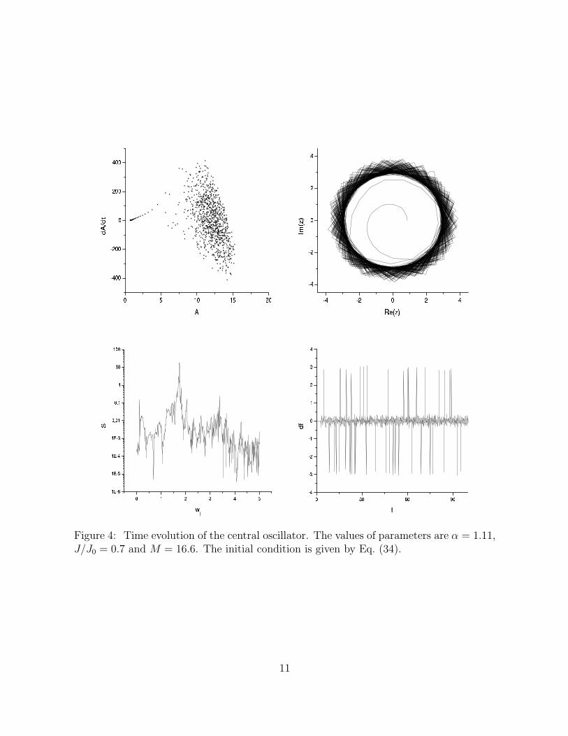
Figure 4: Time evolution of the central oscillator. The values of parameters are α = 1.11,J/J0 = 0.7 and M = 16.6. The initial condition is given by Eq. (34).

11

Figure 5: Surfaces |ψn(t)|2 for the same values of parameters as in Figs. 1-4: α = 1.11,J/J0 = 0.7 and M = 12.5 (top left), M = 14.28 (top right), M = 14.92 (bottom left) andM = 16.6 (bottom right).

12

Our main goal is to compare solutions of Eq. (25) for different values of α ∈ (1, 2) andconsider transition to chaotic dynamics of the chain of oscillators as a function of α. The largeris M , the stronger is nonlinearity. The larger is α, the smaller is LRI. The main differences inthe physical properties of the oscillators dynamics are defined by a competition between α andM . In all simulations we fix J/J0 = 0.7 as the value close to the one considered in [32]. Allplots will show the following properties of the oscillators: plane (dA/dt,A) shows projection ofthe trajectory of the central oscillator in phase space (see definition in (29)); plane (Im z,Re z)shows projection of the complex amplitude z = ψ(0, t) of the central oscillator as a function oftime; phase difference with the adjacent oscillator to the central one (see Eq. (30)); spectrum oftime oscillations of ψ(0, t) (see definition in Eq. (33)); and surfaces |ψn(t)|2 vs t and n.

First four Figures 1-4 aim to show different regimes of the chain of oscillators behavior forα = 1.11. For small values of M solutions are quasi-periodic in time with only few modes inthe Fourier spectrum. This behaviour for M = 12.5 is shown on Fig. 1. The plane (dA/dt,A),the plane (Im z,Re z) and the phase difference plane demonstrate quasi-periodic behavior. Aswe increase the value of M , the spectrum is broadening. Figure 2 demonstrates the behaviourof the system with α = 1.1, J/J0 = 0.7 and M = 14.28. The quasi-periodic structure of theplane (dA/dt,A), the plane (Im z,Re z) and the phase difference plane get more complex.More and more Fourier modes appear in the spectrum. This is even more pronounced forthe case M = 14.92 depicted in Fig. 3, which can be considered as a begining of chaos. Thephase difference of two nearby oscillators shows two ’flips’ to π and −π which indicates phasedecoherence and transition to chaos. In Fig. 4 for M = 16.6 the phase difference of two nearbyoscillators has many ’flips’ to π and −π and the Fourier spectrum of ψ(0, t) becomes broad whatis typical for chaotic dynamics. Surfaces |ψ(x, t)|2 for the cases of Figs. 1-4 are shown in Fig. 5.In addition to the chaotization of the solution which was described above, it is seen that withincreasing values of M , surfaces become more localized around x = 0, oscillations in the wingsof the solutions gradually decrease and the aplitude of the solution is increased. This can beexplained by the growth of the nonlinear term with the growth of M . The role of a nonlinearcoupling becomes more important than coherent connection of oscillators due to the LRI.

Increasing of α leads to appearence of chaotic dynamics for smaller M , without significantchanges of the diagrams and planes shown in Figs. 1-5. This is demonstrated for α = 1.91 inFig. 6. For α = 1.51 chaos starts at approximately M = 14.28 and for α = 1.91 at M = 12.5.Dynamics for α < 1 is approximately similar to the dynamics for 1 < α < 2 and transition tochaos for α = 0.73 occurs at M ∼ 18. The growth of α leads to the increasing of the energy ofoscillations in the tails of the solutions. Transition to the strongly developed chaos is not toosharp in time.

All these results could be compared to the standard DNLS equation with the nearest-neighbor interaction. Solution of this equation with the symmetric initial condition Eq. (34)is shown in Fig. 7 for M = 12.5. There are several main distinctions of this case from thetransition to chaos when α < 2: (i) the symmetry of the solution breaks down for larger M andsharply in time; (ii) the spatial chaos occurs visually earlier than in the case of α < 2, and thisindicates the role of LRI comparing to the standard case of the nearest-neighbor interaction; (iii)another important difference of the onset of chaos in αDNLS and in DNLS can be deduced fromthe (Im z, Re z) plots; in Fig. 7 (top right panel) for DNLS, trajectory fills space more-or-lessuniformly what is typical for Hamiltonian chaos, while in Figs. 3, 4 for αDNLS trajectorieslooks like in the case of stochastic attractors what is more natural for α < 2 [56]. There existsan inner part of the diagram that is avoided by the trajectories, at least for the observed time.

13

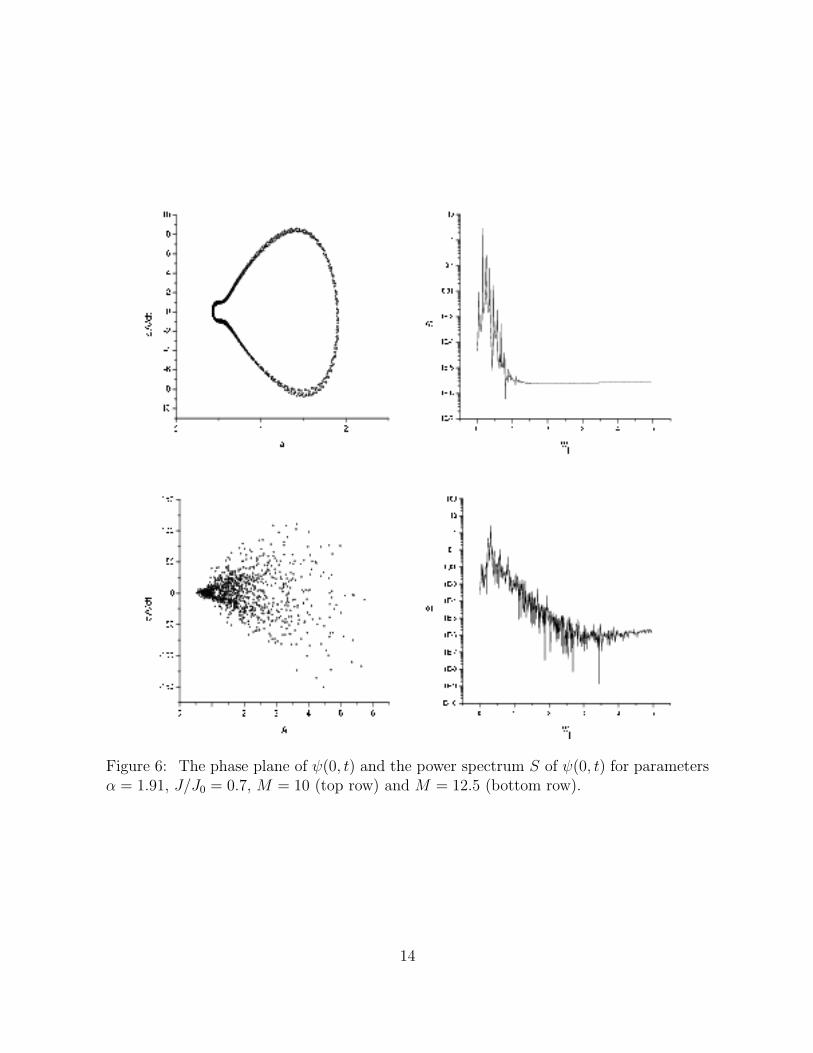
Figure 6: The phase plane of ψ(0, t) and the power spectrum S of ψ(0, t) for parametersα = 1.91, J/J0 = 0.7, M = 10 (top row) and M = 12.5 (bottom row).

14

−5

0

5 0

20

40

60

80

100

0

2

4

6

tx

|ψn|2

-3 -2 -1 0 1 2

-2

-1

0

1

2

3

Im(z

)

Re(z)

0 1 2 3 4 5 6 7 -20

-15

-10

-5

0

5

10

15

dA

/dt

A

0 1 2 3 4 5 1E-10

1E-9

1E-8

1E-7

1E-6

1E-5

1E-4

1E-3

0.01

0.1

1

10

S

w j

Figure 7: Solution of the standard DNLS equation with M = 12.5 and J/J0 = 0.7. Theinitial condition given by Eq. (34).

15

−5

0

5 0

20

40

60

80

100

0

2

4

6

tx

|ψn|2

-2 -1 0 1 2 -2

-1

0

1

2

Im(z

)

Re(z)

0 1 2 3 4 5 -80

-60

-40

-20

0

20

40

60

80

dA

/dt

A

0 1 2 3 4 5 1E-10

1E-9

1E-8

1E-7

1E-6

1E-5

1E-4

1E-3

0,01

0,1

1

10

S

w j

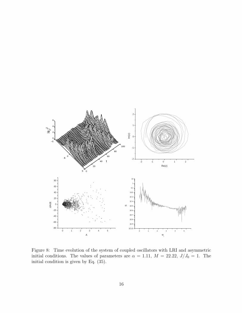
Figure 8: Time evolution of the system of coupled oscillators with LRI and asymmetricinitial conditions. The values of parameters are α = 1.11, M = 22.22, J/J0 = 1. Theinitial condition is given by Eq. (35).

16

The last considered case is the asymmetric initial condition given by Eq. (35). Numericalsolution of the equations of motion reveals a difference in this case compared to the symmetricinitial condition case. For some values of the excitation number M the numerical solution startsto move in the left or right dirrection. This dirrection can also change randomly in time. Figure8 shows an example of such behavior for α = 1.11, J/J0 = 1 and M = 22.22. Note, that thepower spectrum in this case is also broad.

4 Conclusion

One of the main feature of the considered αDNLS model is implementation of a new, additionalto the standard DNLS, parameter α that in the continuous limit implies the fractional dynamicsdescribed by the FNLS. From another point of view, α is responsible for stong correlationsbetween distant oscillators, i.e. a long-range interaction is introduced through the parameterα. This feature of the αDNLS brings a new physics with a new control parameter. The roleof the LRI was known before for collective phenomena in complex medium such as chemical orbiological set of objects [57], phase transition in one-dimentional systems [58], synchronization[23], regularization in quantum field theory [48]. Our detailed analysis helps to understand somespecific properties of destabilization and onset of chaos in αDNLS with α < 2. Similar analysiscan be performed for other models with LRI. An important part of our analysis is utilizationof the possibility to transfrom the behavior of discrete chain of interaction objects into thecontinuous medium equation with the fractional derivatives. This formal procedure raise thequestion of the discrete-continuous equivalence up to a new level where the appearance of anadditional parameter α increases the difficulty the answer the equation.

Acknowledgments

The authors are grateful to V.E. Tarasov for valuable comments and for the reading of themanuscript. This work was supported by the Office of Naval Research, Grant No. N00014-02-1-0056 and the NSF Grant No. DMS-0417800.

References[1] Y.S. Kivshar, D.E. Pelinovsky, Self-focusing and transverse instabilities of solitary waves,

Phys. Rep. 331 (2000), 117-195.[2] S. Flach, C.R. Willis, Discrete breathers, Phys. Rep. 295, (1998) 181-264.[3] D. Henning, G.P. Tsironis, Wave transmission in nonlinear lattices, Phys. Rep. 307, (1999)

333-432.[4] P.G. Kevrekidis, K.O. Rasmussen, A.R. Bishop, The discrete nonlinear Schrodinger equa-

tion: A survey of recent results, Int. J. Mod. Phys. B 15 (2001) 2833-2900.[5] J.C. Eilbeck, M. Johansson, The Discrete Nonlinear Schrodinger equation - 20 Years on,

Proc. of the 3rd Conf. Localization & Energy Transfer in Nonlinear Systems, ed L Vazquezet al (World Scientific, New Jersey, 2003), pp. 44-67.

[6] O.M. Braun, Y.S. Kivshar, Nonlinear dynamics of the Frenkel-Kontorova model. Phys. Rep.306, (1998) 2-108.

[7] D. Cai, D.W. McLaughlin, J. Shatah, Spatiotemporal chaos and effective stochastic dy-namics for a near-integrable nonlinear system, Phys. Lett. A 253, (1999) 280-286.

17

[8] D. Cai, D.W. McLaughlin, Chaotic and turbulent behavior of unstable one-dimensionalnonlinear dispersive waves, J. Math. Phys. 41, (2000) 4125-4153.

[9] D. Cai, D.W. McLaughlin, J. Shatah, Spatiotemporal chaos in spatially extended systems,Math. Comput. Simulat. 55, (2001) 329-340.

[10] B.M. Herbst, M.J. Ablowitz, Numerically induced chaos in the Nonlinear Schrodinger equa-tion, Phys. Rev. Lett. 62, (1989) 2065-2068.

[11] M.J. Ablowitz, B.M. Herbst, On homoclinic structure and numerically induced chaos forthe Nonlinear Schrodinger equation, SIAM J. Appl. Math. 50, (1990) 339-351.

[12] M.J. Ablowitz, C.M. Schober, B.M. Herbst, Numerical chaos, roundoff errors, and homo-clinic manifolds, Phys. Rev. Lett. 71, (1993) 2683-2686.

[13] M.J. Ablowitz, B.M. Herbst, C.M. Schober, Computational chaos in the nonlinearSchrodinger equation without homoclinic crossings, Physica A 228, (1996) 212-235.

[14] M.J. Ablowitz, B.M. Herbst, C.M. Schober, Discretizations, integrable systems and com-putation, J. Phys. A: Math. Gen. 34, (2001) 10671-10693.

[15] D.W. McLaughlin, C.M. Schober, Chaotic and homoclinic behavior for numerical discretiza-tions of the nonlinear Schrodinger equation, Physica D 57, (1992) 447-465.

[16] A. Calini, N.M. Ercolani, D.W. McLaughlin, C.M. Schober, Mel’nikov analysis of numeri-cally induced chaos in the nonlinear Schrodinger equation, Phys. D 89, (1996) 227-260.

[17] G.M. Zaslavsky, Physics of Chaos in Hamiltonian Dynamics, Imperial College Press, 1998(London).

[18] G.A. Baker, Jr., One-dimensional order-disorder model which approaches a second-orderphase transition, Phys. Rev. 122, (1961) 1477-1484.

[19] M. Kac, E. Helfand, Study of several lattice systems with long-range forces, J. Math. Phys.4, (1963) 1078-1088.

[20] Y. Ishimori, Solitons in a one-dimensional Lennard-Jones lattice, Prog. Theor. Phys. 68(1982) 402-410.

[21] A.J. Majda, D.W. McLaughlin, E.G. Tabak, A one-dimensional model for dispersive waveturbulence, J. Nonlinear Sci. 6, (1997) 9-44.

[22] D. Cai, A.J. Majda, D.W. McLaughlin, E.G. Tabak, Dispersive wave turbulence in onedimension, Phys. D 152153, (2001) 551-572.

[23] V.E. Tarasov, G.M. Zaslavsky, Fractional dynamics of coupled oscillators with long-rangeinteraction, Chaos 16, (2006) 023110.

[24] J.A. Sepulchre, A. Babloyanz, Controlling chaos in a network of oscillators, Phys. Rev. E48, (1993) 945-950.

[25] S. Flach, Breathers on lattices with long range interaction, Phys. Rev. E. 58, (1998) R4116-R4119.

[26] V.L. Pokrovsky, A. Virosztek, Long-range interactions in commensurate-incommensuratephase-transition, J. Phys. C 16, (1983) 4513-4525.

[27] G. Alfimov, T. Pierantozzi, L. Vazquez, in: A. Le Mehaute, J.A. Tenreiro Machado, L.C.Trigeassou, J. Sabatier (Eds.), Fractional differentiation and its applications, Proceedingsof the IFAC-FDA’04 Workshop, Bordeaux, France, July 2004; pp. 153-162.

[28] D.W. McLaughlin, C.M. Schober, Homoclinic manifolds and numerical chaos in the non-linear Schrodinger equation, Math. Comp. Siml. 37, (1994) 249-264.

[29] B.M. Herbst, M.J. Ablowitz, Numerical Chaos, Symplectic Integrators, and ExponentiallySmall Splitting Distances, J. Comp. Phys. 105, (1993) 122-132.

[30] B.M. Herbst, F. Varadi, M.J. Ablowitz, Symplectic methods for the nonlinear Schrodingerequation, Math. Comp. Siml. 37, (1994) 353-369.

18

[31] M.J. Ablowitz, B.M. Herbst, C.M. Schober, The nonlinear Schrodinger equation: Asym-metric perturbations, traveling waves and chaotic structures, Math. and Computers inSimulation 43, (1997) 3-12.

[32] Y.B. Gaididei, S.F. Mingaleev, P.L. Christiansen, and K.Ø. Rasmussen, Effects of nonlocaldispersive interactions on self-trapping excitations, Phys. Rev. E 55(5), (1997) 6141-6150.

[33] M. Johansson, Y.B. Gaididei, P.L. Christiansen, and K.Ø. Rasmussen, Switching betweenbistable states in a discrete nonlinear model with long-range dispersion, Phys. Rev. E 57(4),(1998) 4739-4742.

[34] K.Ø. Rasmussen, P.L. Christiansen, M. Johansson, Y.B. Gaididei, S.F. Mingaleev, Local-ized excitations in discrete nonlinear Schrodinger systems: Effects of nonlocal dispersiveinteractions and noise, Physica D 113 (1998) 134-151.

[35] P.L. Christiansen, Y.B. Gaididei, F.G. Mertens, S.F. Mingaleev, Multi-component structureof nonlinear exitations in systems with lenth-scale competition, Eur. Phys. J. B 19, (2001)545-553.

[36] Y.B. Gaididei, S.F. Mingaleev, P.L. Christiansen, and K.Ø. Rasmussen, Effects of nonlocaldispersion on self-trapping excitations, Phys. Lett. A 1996 152-156.

[37] H. Weitzner, G.M. Zaslavsky, Some applications of fractional derivatives, Commun. Nonlin.Sci. Numer. Simul. 8, (2003) 273-281.

[38] A.V. Milovanov, J.J. Rasmussen, Fractional generalization of the Ginzburg-Landau equa-tion: an unconvential approach to critical phenomena in complex media, Phys. Lett. A337, (2005) 75-80.

[39] N. Laskin, G.M. Zaslavsky, Nonlinear chain dynamics with long-range interaction, PhysicaA 368, (2006) 38-54.

[40] V.E. Tarasov, G.M. Zaslavsky, Fractional Ginzburg-Landau equation for fractal media,Physica A 354, (2005) 249-261.

[41] V.E. Tarasov, Psi-series solution of fractional Ginzburg-Landau equation, J. Phys. A. 39,(2006) 8395-8407.

[42] S.G. Samko, A.A. Kilbas, O.I. Marichev, Fractional Integrals and Derivatives Theory andApplications, Gordon and Breach, New York, 1993.

[43] N. Korabel, G.M. Zaslavsky, V.E. Tarasov, Coupled oscillators with power-law interactionand their fractional dynamics analogues, in press, Commun. in Nonlin. Sci. and Comput.Simulations, (2006).

[44] R.P.A. Lima, M.L. Lyra, J.C. Cressoni, Multifractality of one electron eigen states in 1Ddisordered long range models, Physica A 295, (2001) 154-157.

[45] D.W. Schaefer, J.E. Martin, P. Wiltzius, et al., Fractal geometry of colloidal aggregates,Phys. Rev. Lett. 52, (1984) 2371-2374.

[46] P. Pfeifer, D. Avnir, Chemistry in noninteger dimensions between two and three. I. Fractaltheory of heterogeneous surfaces, J. Chem. Phys. 79, 3558-3565.

[47] E. Goldfain, Derivation of the fine structure constant using fractional dynamics, Chaos,Solitons and Fractals 17 (2003) 811-818.

[48] E. Goldfain, Renormalization group and the emergence of random fractal topology in quan-tum field theory, Chaos, Solitons and Fractals 19 (2004) 1023-1030.

[49] E. Goldfain, Complexity in quantum field theory and physics beyond the standard model,Chaos, Solitons and Fractals 28 (2006) 913-922.

[50] A. Erdelyi, W. Magnus, F. Oberhettinger, F.G. Tricomi, Higher Transcendental Functions,Vol. 1, New York, Krieger, (1981) pp. 30-31.

19

[51] L. Lewin, Polylogarithms and associated functions, New York: North-Holland; 1981.

[52] K.B. Oldham, J. Spanier, The Fractional Calculus, Academic Press, New York, 1974.

[53] K.S. Miller, B. Ross, An Introduction to the Fractional Calculus and Fractional DifferentialEquations, Wiley, New York, 1993.

[54] I. Podlubny, Fractional Differential Equations, Academic Press, New York, 1999.

[55] F. Mainardi, R. Gorenflo, Feller fractional diffusion and Levy stable motions, in: O.E.Barndorff-Nielsen, S.E. Graversen, T. Mikosch (Eds.), Proceedings of the InternationalConference on ”Levy Processes: Theory and Applications”, MPS-misc. 1999-11, pp. 11-122,

[56] G.M. Zaslavsky, A.A. Stanislavsky, M. Edelman, Chaotic and pseudochaotic attractors ofperturbed fractional oscillator, CHAOS 16 (2006), 0131021-0131026.

[57] Y. Kuramoto, Self-entrainment of a population of coupled non-linear oscillators. in In-ternational Symposium on Mathematical Problems in Theoretical Physics. Ed. H. Araki(Springer, Berlin, 1975) pp.420-422.

[58] F.J. Dyson, Existence of a phase-transition in a one-dimensional Ising ferromagnet. Com-mun. Math. Phys. 12 (1969) 91-107; Non-existence of spontaneous magnetization in a one-dimensional Ising ferromagnet. Commun. Math. Phys. 12 (1969) 212-215; An Ising ferro-magnet with discontinuous long-range order. Commun. Math. Phys. 21 (1971) 269-283.

20