Chaos, add infinitum

Hayden Wilkinson∗

Last updated: August, 2021Comments welcome: hayden.wilkinson@anu.edu.au

Abstract

Our universe is both chaotic and, most likely, infinitely large. This presents problems for moral

decision-making. The first: due to our universe’s chaotic nature, our actions often have long-lasting,

unpredictable effects; and this means we typically cannot say which of two actions will turn out best

in the long run. The second problem: due to the universe’s infinite dimensions, and infinite population

therein, we cannot compare outcomes by simply adding up their total moral values—those totals will

typically be infinite or undefined. Each of these problems poses a threat to aggregative moral theories.

And, for each, we have solutions: a proposal from Greaves let us overcome the problem of chaos,

and various proposals from the infinite aggregation literature let us overcome the problem of infinite

value. But a further problem emerges. If our universe is both chaotic and infinite, those solutions no

longer work—outcomes that are infinite and differ by chaotic effects are incomparable, even by those

proposals. In this paper, I show that this further problem can be overcome. But, to do so, we must

accept some peculiar implications about how aggregation works.

Keywords: infinite aggregation; chaos theory; cluelessness; infinite utility streams; infinite value;

∗Global Priorities Institute, University of Oxford

1 Introduction

Consider a seemingly simple moral decision. While out walking, you see a child stepping onto the road to

cross to the other side. Until recently, this was a one-way street. And it seems the child does not know

that traffic now runs both ways, because they are looking in just one direction. Meanwhile, a long line of

traffic bears down on them from the other direction. If the child continues crossing, they will clearly be

squashed by the leading vehicle. (Perhaps you can see that the driver is rummaging in their glove-box,

oblivious to the child before them.) But, fortunately, you are not far from the child. If you dash forward,

you can grab them just in time. If you do, they will be saved. If you do not, they will die.

You may have various reasons to save the child, and perhaps reasons not to. But let us focus on just

one source of reasons: how good the outcome of each action would be. It seems obvious that the outcome

in which the child survives will be better than that in which they die—the former will contain more moral

value overall, resulting from that child going on to enjoy the rest of their (presumably good) life.

But will it? Will saving the child produce an outcome with greater moral value? In reality, it likely will

not, thanks to two quirks of our physical setting. The first is that saving the child has causal ramifications

far beyond producing just one additional life worth living. To see why, note that many of the physical

systems we interact with on a daily basis are chaotic. As a result, small interventions on those systems

typically result in wildly different outcomes in the future. One such system, if you are in a sufficiently

dense city, is traffic flow (see Lighthill and Whitham, 1955). By allowing or preventing the child being

hit by that car, you would allow or prevent a temporary standstill in traffic on that street. Over the

following hours, this would alter traffic flow throughout the system, momentarily delaying or advancing

countless other drivers. Depending on the size and density of your city, this would change which other

traffic accidents occur and where. Beyond this, saving the child means that they will continue their life,

with all the street-crossing and driving they ever do, and so you will alter the traffic flow on countless

other evenings. Likewise for the street-crossing done by every one of the child’s descendants. Effectively,

by saving that child, you have caused and prevented many, many other traffic accidents and the resulting

deaths, likely far outweighing the value of the child’s life. And that’s merely through disrupting traffic,

rather than the disruptions you cause to many other chaotic systems (see Section 2). So you cannot be

confident that saving the child will result in an outcome of greater total value. So you will be clueless as

to whether it is better to save the child or not (see also Greaves, 2016; MacAskill and Mogensen, 2021).

And this is deeply counterintuitive—intuition suggests that saving the child is clearly better.

Chaos is one problem for comparing outcomes by their total values. Here is another: our universe

may be infinitely large, or so the current science suggests. In light of recent developments in cosmology,

we should expect that, no matter what actions we take, the future will contain infinitely many morally

valuable lives.1 So too should we expect that, no matter what we do, those lives will include infinitely1This is implied by both the constant cosmological constant model (Wald, 1983; Carroll, 2017) and the inflationary view

(Garriga and Vilenkin, 2001), each of which is widely accepted among physicists and well-supported by the current body ofevidence. Each predicts that our physical universe is infinite in momentary spatial volume and/or temporal duration. Theyalso each predict that the local events across an infinite sub-region of our universe will consist of effectively random events.(By the constant cosmological constant model, this region is populated by statistical fluctuations from a cold, high-entropystate.) And across such a sub-region of infinite volume, we should expect every physically possible state to arise infinitelymany times. So take any small-scale phenomenon you might think is morally valuable e.g., a human brain processing asensation of intense pleasure. Over our universe with its infinite volume, we should expect identical such brains to arise

1

many quite good ones (with value greater than some ε > 0, on some cardinal scale), and infinitely many

quite bad ones (with value less than −ε). In the above case, whether you save the child or not, there will

be infinitely many quite good lives and infinitely quite bad lives. Which outcome contains more value?

In some sense, neither. For each, we have an infinite subtotal of positive value and an infinite subtotal

of negative value (on whichever cardinal scale is used)—with those summed together, the final total is

undefined. We cannot say that either total value is greater, or less, than the other. Plausibly, this means

that we cannot say that either outcome is better ; the two outcomes are incomparable. And, as before, this

is deeply counterintuitive—the outcome of saving the child seems clearly better.

Both of these problems threaten moral theories that are aggregative with respect to value: those

that say that an outcome is better than another if and only if it contains a greater total aggregate of

moral value, impartially construed. (The betterness of options, or lotteries over outcomes, may be a little

more complicated—see §2.4 and §4.) Given the nature of our universe—both chaotic and infinitely large—

aggregative moral theories often cannot say that one outcome is better than another, even when the correct

verdict seems obvious. This is particularly worrying if the correct moral theory is not just aggregative but

also purely consequentialist—if, in all decisions, you ought to perform whichever available action will result

in the best outcome (or, under uncertainty, the best lottery over outcomes). If so, it seems that we cannot

say that you ought to save the child. But even if the correct theory is not purely consequentialist, most

plausible ethical theories rely on the betterness of outcomes to make at least some judgements—most say

that, if an action brings about a greater total aggregate of value than the alternatives do, that provides

at least pro tanto reason to choose it. Throughout this paper, I will focus on theories that recognise at

least that pro tanto reason. And such theories will have trouble dealing with the above problems of chaos

and infinite value—they will often struggle to say that one outcome is better than another, even in cases

as simple as deciding whether to stop a child from walking into traffic. Given this result, it seems that we

should reject all such aggregative theories.

But, fortunately, we may not need to. We have some aggregative theories that overcome each of

the problems raised above. We have proposals for aggregative theories that compare our options despite

chaotic effects (see Section 2). And there have been a variety of aggregative theories proposed to overcome

the problem of infinite value. These theories of infinite aggregation each step away from representing the

total value of each world as a single real-valued sum, but instead as some other mathematical object (see

Vallentyne, 1993; Vallentyne and Kagan, 1997; Lauwers and Vallentyne, 2004; Bostrom, 2011; Arntzenius,

2014; Wilkinson, 2021, and Askell 2019 for a survey). We’ll see several of these in action in Section 3.

But we face a further, as yet unexplored, problem. If our universe is both infinite and widely chaotic, we

face a greater challenge. Our solutions to the problem of chaos fail if outcomes also contain infinite value.

And (most of) our solutions to the problem of infinitude fail as well—they cannot compare outcomes that

differ by lasting chaotic effects, ad infinitum, and so cannot compare any pair of outcomes ever available to

us. In the decision of whether to save the child or not, most of our existing methods say that the outcomes

are incomparable. Neither is better. And, if the value of outcomes is all that weighs in favour of either

choice, we have no reason to choose one rather than the other. And the same holds in many of the moral

decisions you or I will ever make. Effectively, chaos and infinite value together undermine a large swathe

infinitely many times (see Carroll 2017 and Davenport & Olum 2010 for further detail).

2

of our moral decision-making.

In this paper, I seek a solution to this further problem. Before that, in Section 2, I’ll explain in greater

depth how our actions almost always result in chaotic, long-lasting changes to the world, far beyond

affecting traffic flows. In Section 3, I’ll lay out the further problem of chaos ad infinitum, demonstrating

how the problem arises for each of several classes of aggregative theories tailor-made for the infinite setting.

I’ll also demonstrate that some (and only some) aggregative theories can avoid the problem. But these

theories will be slightly peculiar. In Section 4, I’ll extend those theories beyond comparisons of chaotic

outcomes to cover comparisons of lotteries over chaotic outcomes. Section 5 is the conclusion.

As we will see, the combined problem of chaos and infinite value sheds light on which, if any, aggregative

theories might be the correct one. After all, only some theories can overcome the problem. But all of

those theories imply something deeply counterintuitive: that comparisons of outcomes can depend on the

positioning of moral value in space and time. You might think this implication unacceptable—surely,

moral evaluations must be independent of precisely who obtains value and where they are located. But

in an infinitely large, chaotic universe, only aggregative theories that violate this independence can make

plausible judgements. And so we have a compelling argument for accepting a peculiar form of aggregative

theory; that or we have a reductio against aggregation, and should abandon it altogether. I will leave it

to you to decide which conclusion to draw.

2 Chaos

Many of the physical systems in our universe are chaotic. Chaos has a technical definition (see Feldman,

2019, p. 83) but, for my purposes, just one of the conditions necessary for a system to be chaotic will be

relevant: that its states at all later times are highly sensitive to its initial states.2 They are highly sensitive

in that if we were to ever-so-slightly alter the properties of the system in the earlier state—sometimes in

an arbitrarily small way—the later states would change in a much more significant way.

Three such chaotic systems are: the composition of the human population; the Earth’s atmosphere;

and the positions of the planets in our solar system. And our actions frequently change all of these, now

and indefinitely far into the future.

2.1 Identities

Recall the case from the beginning. If you save the child from walking into traffic, they will live out the

rest of their life, likely have children of their own, likely have grandchildren, and so on. If they would

have a long line of descendants, your choice changes whether or not those descendants come to exist. You

would thereby change the composition of the human population well into the future.2Of course, a system need not be chaotic for its later states to be highly sensitive to initial conditions. Systems that are

not chaotic may even be more sensitive to those conditions—as Gleick (1987, p. 292) points out, given the attractor statesobserved in chaos theory, chaotic systems often follow similar large-scale patterns regardless of what happens at a small scale.But the systems I describe here are all genuinely chaotic ones (in the non-technical sense too). And, although their chaoticnature is not necessary for demonstrating the problem I have in mind, it is sufficient. (Less importantly, the phrase ‘sensitivedependence to initial conditions’ is far less catchy than simply ‘chaos’.)

3

How likely is it that that child would spawn a long line of descendants? Very likely, it turns out. At

least in the United Kingdom, 97.9% of 5-year-old children live to at least 45 (Office for National Statistics,

2019). And, by the age of 45, 82% of people in England or Wales have had at least one child (Office for

National Statistics, 2018). If the child is 5 years old and current rates hold3, it can be shown that the

child’s lineage will last forever, in expectation. Not just that, but the probability that they have some

genetic descendants at a given time (conditional on humanity still existing) quickly approaches 0.7.4 So

there is a probability of at least 0.7 that your choice in that situation will change the genetics of some

portion of humans for as long as humanity exists.

And this will change the events that happen in those descendants’ lives and the lives of those they

interact with. With differences in genetics come countless differences in heritable traits, including height,

body mass index (Wainschtein et al., 2019), intelligence (Plomin and Deary, 2015), empathy (Melchers

et al., 2016), and plenty of others. At least some of these traits greatly affect the quality of one’s own life

and the lives of others. So significantly changing the genetic composition of humanity millennia into the

future will also, at least occasionally, affect the moral value that particular humans obtain and the times

at which they obtain it.

But the identity effects of your choice go far beyond this. As noted earlier, saving that child would

cause rippling changes throughout the city’s traffic system, changing the positions of many other vehicles

throughout the remainder of their journeys. Some number of lucky drivers on the road that day would be

on their way home to conceive a child. By delaying or advancing their arrival home, you almost certainly

alter the moment at which conception occurs. And, as pointed out by Parfit (1984, ch. 16) and Greaves

(2016), this will almost certainly alter which sperm fertilises the egg, and so too the genetics of the resulting

child. And, just like the child you saved to begin with, the newly conceived child will likely spawn an

indefinitely long line of descendants. So too will the slightly different actions of that newly conceived child

and all of their descendants cause similar changes, e.g., slightly delaying traffic when they cross a street.

And so the identity changes resulting from your original choice will ripple ever outwards.

2.2 Weather patterns

Another archetypal chaotic system, and one which we constantly interact with, is the Earth’s atmosphere.

It was this system, and its behaviour under small perturbations, that first inspired Edward Lorenz’ work3Current rates may not hold, but they are still a reasonably good predictor of future rates. We can anticipate that UK

birth rates will be a particularly good lower bound, as a highly developed, wealthy country. And if the long-run mean numberof births were to drop much lower—below 2—humanity would die out.

4From ONS (ibid), by the age of 45, 18% of Britons have had no children, 18% have had 1 child, 37% have had 2, 17%have had 3, and 10% have had 4 or more. And from ONS (2019), 97.4% of Britons live to the age of 45. For simplicity,I’ll assume that no one has children after the age of 45. And, conservatively, I’ll assume that no one who dies before 45has any children, everyone who has 4 or more children just has 4, and that the child’s descendants aren’t any more likely tohave (many) children just because their forebears did. Then, conditional on that first child living to 45, we can representthe number of their descendants in each subsequent generation n by Zn =

∑Zn−1i=1 Xi, where the Xis are independent,

identically-distributed random variables with P (Xi = 0) = 0.201, P (Xi = 1) = 0.175, P (Xi = 2) = 0.360, P (Xi = 3) = 0.166,and P (Xi = 4) = 0.097.

This is what is called a Galton-Watson process. As such, the probability of any descendants remaining by generation n isgiven by P (Zn > 0) = 0.201+0.175×P (Zn−1 > 0)+0.36×P (Zn−1 > 0)2 +0.166×P (Zn−1 > 0)3 +0.097×P (Zn−1 > 0)4

(Grimmett and Stirzaker, 1992, §5.4). That probability converges to p as n → ∞ if there is some p such that P (Zn > 0) =P (Zn−1 > 0) = p solves that equation. Here, it does, for p = 0.715. Multiplying that by the probability that the first childlives to 45 (0.979), we have a probability of (at least) 0.700 that the child has descendants for as long as humanity survives.

4

on chaos theory (e.g. Lorenz, 1963).

Suppose again that you save the child from traffic. By doing so, you will move your (and their) body

and disturb the air around you, making the air flow around you ever-so-slightly different. The oncoming

traffic will continue unhindered, changing the movement of air in your vicinity even more. Likewise, your

action will result in the child continuing to go about their life for many years, disturbing the air around

them with every movement they make.

But even quite small disturbances to the air within the Earth’s atmosphere results in major, unpre-

dictable changes to weather patterns indefinitely far into the future (ibid). Lorenz (1972) claimed, iconi-

cally, that even changing whether and when a butterfly in Brazil flaps its wings is often enough to change

whether and when a tornado occurs in Texas. As Broome (2019) points out, Lorenz may be wrong—it

is unclear whether the effects of a mere butterfly flap would spread, given the viscosity of air—but it is

clear that larger-scale disturbances have this effect (Palmer et al., 2014). Some disturbances include: each

human breath, which releases 140 times as much energy as a butterfly’s wing flap; and running an electric

fan for a single second, which releases 10 million times as much.5

Save the child and you change whether, when, and where countless human breaths, uses of electric

fans, and other atmospheric disturbances take place. So you affect the timing and location of tornadoes,

cyclones, wind gusts, rainfall, and so on indefinitely far into the future. And likewise by affecting the lives

of the child’s descendants—they too would breathe, use fans, and so on. And tornadoes and other weather

events have significant effects on the lives of many people. So your choice continues to affect the moral

value that arises indefinitely far into the future.

2.3 Planetary motion

Yet another chaotic system is the position of the planets in our solar system, each under the gravitational

influence of the others (Malhotra et al., 2001).6

Note that, if you save the child, their body to continue moving about the Earth’s surface for decades,

rather than perhaps remain stationary in a cemetery. (So too will many objects they interact with move

about the Earth’s surface.) But, as an object with mass, their body casts a gravitational field. Move

a human body and that field changes. At the most extreme, that body might move from one side of

the Earth to the other. This slightly changes the Earth’s distribution of mass. And this distribution is

important—since the Earth’s mass occupies more than a single point, the strength of the gravitational

field from other planets and celestial bodies will differ from one side of the Earth to the other. So changing

the distribution of mass can change the gravitational force applied to the Earth and its inhabitants. Just

from the gravitational field exerted by Mercury (the planet most often closest to the Earth), moving an

80 kilogram human body from one side of the Earth to the other has an effect equivalent to changing the

Earth’s mass by 1.6 milligrams.7 Over the course of 24 hours, that results in the Earth’s position changing5These ratios are calculated from figures given in Dasgupta (2008, p. 78-9), Putensen and Wrigge (2007), Tang et al.

(2013), and the packaging of an electric fan I had on hand.6In fact, it was while studying a similar system that Henri Poincaré (1890) inadvertently laid the foundations for chaos

theory.7The calculation for this is somewhat complex, but follows from the following facts: the gravitational force exerted on one

5

by 4× 10−30 metres (or 40 attometres).

That distance may seem trivial. But small disturbances in the positions of celestial bodies in our solar

system lead to large changes, at least over long periods of time. If the Earth’s position is shifted by some

distance now, it is overwhelmingly likely that its future position is shifted by an even greater distance,

although we cannot predict exactly where it will end up. Typically, if you shift the Earth by 4 × 10−30

metres today, you will typically cause a 4 metre difference in the Earth’s position in 300 million years (see

Laskar, 1989)—still trivial, perhaps. But wait another 120 million years and the difference will typically

grow to about 4 billion kilometres (ibid). For reference, that is roughly the distance of Neptune from the

sun. And, as you might guess, this would have major effects on what occurs on Earth—for comparison,

the full range of temperature variations we experience each year are a result of varying our distance from

the sun by a mere 5 million kilometres.

That’s the effect of moving a human body from one side of the planet to the other for a day. But

similar, smaller effects occur if the child you save (and/or their descendants) spends a day in another city

or country. The initial difference in the Earth’s position will be smaller but, over long enough time spans,

it will grow just as large. And this applies not just to the Earth’s position—the bodies in our solar system

also exert gravitational fields on neighbouring systems and beyond. Over long enough time spans, these

changes ripple out to affect other systems, any civilisations that inhabit them, and any moral value that

arises there. By this route, your choice of whether to save the child affects events indefinitely far into the

future and into remote space.8

2.4 The problem of cluelessness

Why are any of these effects a problem for our moral evaluations?9

In the same case as before, if you let the child die then the future will proceed in one particular way.

If you save them, the future will proceed very differently: the genetic composition of much of humanity,

the Earth’s weather patterns, and the trajectories of our planet and others will all be altered. These

alterations will be significant and will last indefinitely far into the future.

To compare these outcomes on an aggregative moral theory, we look to their total values. (Assume for

now that these are finite.) We can obtain each outcome’s total value by summing the value it contains

during each consecutive interval of time. For instance, if we let O1 be the outcome resulting from letting

the child die, and O2 the outcome resulting from saving them, each outcome will have some value (Xi or

object with mass m1 by another of mass m2 and at distance r is given by F = 6.674× 10−11 × m1m2r2

; the Earth has a massof 5.972 × 1024 (kilograms); Mercury has a mass of 3.285 × 1023 and lies at an average distance of 7.7 × 1010 metres fromthe Earth; and the Earth’s radius (and so the rough distance of the 80kg human from the centre) is 6.371× 106.

8This continues to hold even if the future lasts infinitely long and contains infinitely many persons. On the constantcosmological constant model mentioned in Footnote 1, infinitely many future persons will be the product of quantum fluc-tuations that arise after our universe enters its ‘heat death’ era. The manner and timing of these fluctuations will beaffected—although not predictably—by even subtle changes in gravity (as by the Hawking effect), electric field strength (asby the Casimir effect), and, plausibly, many other factors too. And we can easily influence the gravitational properties of aninfinite region of points in the post-heat-death vacuum—by radically changing the positions of planets and star systems overmillions of years, as described above, we would produce gravitational changes that ripple outwards in spacetime, infinitelyfar into the future. So the choice to save the child from traffic, for instance, would continue to have ramifications infinitelyfar into the future.

9The basic argument given here originates with Lenman (2000) and the formal aspects with Greaves (2016).

6

Yi) arise at each future time (ti).

t0 t1 t2 t3 t4 t5 t6 ... tN

O1 : X0 X1 X2 X3 X4 X5 X6 ... XN

O2 : Y0 Y1 Y2 Y3 Y4 Y5 Y6 ... YN

For O2 to be a better outcome than O1 is for the sum of Y0 up to Yn to be greater than the sum of X0

to Xn; or, equivalently, for the sum of the differences Y0 −X0 up to Yn −X0 to be greater than 0. And

what would those differences be? To simplify matters, we can suppose that the only difference in value at

t0 is whether the value in the life of that child—represented as value 1—occurs or not. Then O2 is better

if and only if:

V (O2)− V (O1) = 1 +

n∑i=1

(Yi −Xi) > 0

But remember that your choice has long-lasting chaotic effects. The values of many of those Xis and

Yis are unpredictable, so you should be uncertain about them. So each Xi and Yi can be treated as

a random variable with some probability distribution.10 These probability distributions may differ for

different times—different Xis and Yis—based on what you do know about the future. But since you have

no reason to think that your action’s chaotic effects will favour one outcome or the other at a given time,

each Yi is distributed identically to its corresponding Xi. So each difference Yi−Xi will have a probability

distribution that is symmetric about 0. Given this, the sum above follows a random walk, and a symmetric

one at that. As we sum the differences Yi −Xi up to some large tn, it will typically look like this.

1

n

V (O2)− V (O1)

Figure 1: The difference in total value between O1 and O2, given by 1 +∑ni=1(Yi −Xi)

Notice that this walk passes above and below 0 sporadically. In fact, any such random walk, generated

from any sum of symmetric, independent, identically-distributed random variables, will continue to return

to 0 no matter how far along the walk we go—no matter how far above or below 0 the sum gets, we

know that such a walk will return to 0 if we just wait long enough, and that it is then just as likely to

rise above 0 as it is to dip below it (Chung and Fuchs, 1951). So, for large n, we cannot predict whether

it will be above or below 0—we have no clue. The theory of random walks tells us that the probability10These distributions may be determined by either your subjective or evidential probabilities. What follows can be read

in terms of either.

7

that V (O2) − V (O1) is positive (or negative) approaches 0.5 as n approaches infinity. In fact, here the

probability already approximates 0.5 for even modest n like 10 or 100, at least given just that one small,

initial difference. But no matter that initial difference, over a long future, it is as likely as not that either

outcome turns out worse.

As it happens, the variables Yi−Xi may not be entirely independent and identically-distributed. After

all, the scale of differences between the two outcomes may grow over time. And some later differences will

be (at least partially) dependent on earlier differences—e.g., if you cause the Earth’s orbital path to pass

nearer to the sun and the resulting increase in temperature does harm, its effects at later times are more

likely to be harmful too. But the above results will still hold—over long enough time spans, the walk will

be guaranteed to return to 0, and the probability of being above (or below) 0 will approximate 0.5.11 So

it will still be as likely as not that either outcome turns out worse than the other.

This seems like bad news for the aggregationist. Even in seemingly simple decisions like this—along

with many decisions in practice—we are radically uncertain as to whether an action will turn out better

than its alternatives. If we make decisions based on our reasons to promote (actual, overall) moral value,

then those reasons seem to give no additional guidance at all.

But this uncertainty isn’t fatal for the aggregationist project. We are deeply uncertain about which

action will actually turn out better, but we may not be uncertain about which action looks better in

expectation, given our uncertainty—we cannot say which action produces a better outcome, but we might

still be able to say which action produces a better lottery over possible outcomes. And we can indeed do

so for cases like this, as Greaves (ibid : 8-9) demonstrates. Take the expectation of the total value for each

outcome, and compare them, as below.

E(V (O2))− E(V (O1))

= E(Y1) + E(Y2) + E(Y3) + ...− E(X1)− E(X2)− E(X3)− ...

= E(1) +n∑i=1

E(Yi −Xi)

= 1

Unsurprisingly, the difference is positive; saving the child brings the greater expected total value. This

is because all that distinguishes the two lotteries from one another is that one brings a certainty of the

child surviving and the other a certainty of their death. As for future events, with values represented by

Xi and Yi, we know nothing of how they will differ; we place the same probabilities on each possible value

of Xi as we do on each possible value of Yi. So of course the difference in their expected values is 0, since

they’re identical. And so, in expectation, the value at every future time cancels out, and all we are left

with is the guaranteed value of the child’s life.

So, if we switch from comparing actions by the whatever total value their actual outcomes contain, to

comparing actions by the total expected values of their lotteries over outcomes, we can say that it is better

to save the child. This is the approach defended by Jackson (1991) and other subjective aggregationists,11For a survey of what are termed reinforced random walks like this, see Pemantle (2007).

8

who would say that the outcome is subjectively better if you save the child, and that this is the normatively

relevant sense of betterness. We may be uncertain of which outcome is objectively better, but that need

not trouble us. So, on at least some aggregative views, we can still say that saving the child is better in a

relevant sense and that you should save them, despite the presence of widespread chaos.12

3 Chaos, with infinite value added

As we saw above, if the universe is finite then chaos poses a problem for aggregation. Unpredictable chaotic

effects lead to uncertainty over which act will actually have the better outcome. But that need not stop

us from making practical judgements—after all, we still know that some outcome will be better (or that

they will be equally good). We just need to respond to uncertainty over which outcome that will be. And

we can do that, by taking the expectations of their (finite) total values.

But if the universe is infinite, chaos poses a greater problem. As we will see, in the infinite context we

are not just uncertain of which act will turn out better. Rather, we are certain that neither act will. We

can say with certainty that the outcomes of any two available acts will be incomparable or else equally

good. Those are the verdicts given by almost every aggregative view that has been proposed in the infinite

setting. So, by those views, we again cannot say which is better—to save the child from walking into

traffic, or to not save them.

How we reach those verdicts will differ according to the aggregative theory we adopt in the infinite

context. We can separate the available theories into three categories: strongly anonymous theories; weakly

anonymous theories; and position-dependent theories. I’ll explain why each of these commits us to implau-

sible verdicts, in turn.

3.1 Strongly anonymous theories

A strongly anonymous theory is one that says that, when comparing one outcome to another, the com-

parison depends only on how many13 persons obtain each level of value. It does not matter which persons

obtain value in each outcome, nor their positions in space and time, their hair colour, their height, nor

any other such qualitative properties except for whether they exist and the level of value they obtain. (See

§3.3 below for further discussion.) So if two outcomes look identical after we censor the identity and those

other qualitative properties of each and every person, then those worlds must be equally good.14

To put this precisely, call a view strongly anonymous if it satisfies the following condition.12The situation is different for objective aggregationist views, such as that defended by Railton (1984). Such objective

aggregationists will still find themselves clueless as to what they should do.13Specifically, I mean the cardinality of each such set of persons, rather than another notion of size like containment or

density.14Strictly speaking, this last claim requires not just Strong Anonymity but also that the ‘at least as good relation is

transitive: for any outcomes Oa, Ob, and Oc, if Oa is at least as good as Ob and Ob is at least as good as Oc, then Oa is atleast as good as Oc. This assumption is ubiquitous for aggregative theories of value, and is defended at length by Broome(2004), Huemer (2008), Nebel (2018), and Dreier (2019).

Take the outcomes Oa and Oa′ from the definition of Strong Anonymity and let Ob be any outcome that is equally asgood as Oa. Strong Anonymity implies that it is equally as good as Oa′ too. Then, by the transitivity of ‘at least as goodas’, Oa and Oa′ are equally good.

9

Strong Anonymity : Let Oa, Ob, and Oa′ be any possible outcomes. If Oa′ can be obtained

from Oa by replacing the identities and qualitative properties of some subset of persons in Oa,

holding fixed the value they each obtain, then Oa is at least as good as Ob if and only if Oa′ is

at least as good as Ob.

When all possible outcomes contain only finitely many persons, Strong Anonymity is satisfied by all

plausible aggregative views. But it is less widely endorsed in the infinite setting. This is because, in the

infinite setting, Strong Anonymity clashes with other highly plausible principles, e.g., the Pareto Over

Persons principle (van Liedekerke, 1995), which I’ll discuss below. As a result, many views reject Strong

Anonymity, including all of the weakly anonymous and position-dependent theories that I mention below.

But at least two authors do still endorse Strong Anonymity in this setting: [omitted for blind review] and

[omitted].

What do strongly anonymous theories say about realistic cases involving chaos? It turns out that they

say cannot say that any outcome is better than any other.

Returning to the case of saving or not saving the child from walking into traffic, we can represent the

two outcomes as below. In each outcome, each person obtains some amount of value. For the child p1,

they obtain value 0 if they die, and 1 if you save them. Then we have some (perhaps finite) number of

persons p2, p3, p4, and so on who are unaffected by your choice and so who obtain the same value in both

outcomes. For those persons, you are (at least somewhat) uncertain of the values they each obtain, given

by random variables X2, X3, and so on, but these are the same in both outcomes. Then we have infinitely

many persons pi, piii, and so on who exist in both outcomes but who are affected by your choice. They also

obtain random values but, importantly, different random values in each outcome (e.g., Xi as against X ′i ).

And then we have two distinct sets of infinitely many persons—pa, pb, etc and pα, pβ , etc—whose existence

is affected by your choice. In one outcome, one of the two groups exists and obtains some random values.

In the other, the other group exists.15

p1 p2 p3 p4 ... pi pii piii ... pa pb pc ... pα pβ pγ ...

O1 : 0 X2 X3 X4 ... Xi Xii Xiii ... Xa Xb Xc ... − − − ...

O2 : 1 X2 X3 X4 ... X ′i X ′ii X ′iii ... − − − ... Xα Xβ Xγ ...

What do we know about each of these random X values, which make up the bulk of the value in the universe?

We don’t know exactly what each of them will be, as each is random. But we do know that each will be drawn

from some probability distribution, perhaps one of those illustrated below.

15Here, we have three infinite subgroups of persons in each world (and possibly four, if {p2, p3, ...} is infinite too). Whywould these all be infinite? The chaotic effects of your action will extend infinitely far into the future. (See Footnote 9above.) These include identity effects, so infinitely many people ({pa, pb, ...} and {pα, pβ , ...}) will exist in each outcome butnot in the other. But, as well, infinitely many persons ({pi, pii, ...}) will have their identities unchanged—for any given futureperson in one outcome, there is at least a non-zero probability that their identity will remain the same regardless of youraction, even if the value they obtain is changed. With infinitely many such persons out there, infinitely many will thereforehave their identities remain unchanged.

10

Value

Proba

bilitydensity

Figure 2: Probability distributions for some random variables Xa, Xb, Xc

We know a few other things about these distributions. For one, we know that at least infinitely many of these

X values will be drawn from distributions that give non-zero probability density to the values 0 and 1. After

all, if these are possible values of the life of that child on the street, then these values are well within the realm

of epistemic possibility for persons in the future and anywhere else in the universe. For two, we know that the

distributions in O1 and O2 will be similar—we should have the same distributions for Xi and X ′i and for Xa and

some corresponding Xα (even their actual value turns out differently). After all, we have no reason to think that a

particular one of the outcomes will be better for each person. For three, it then follows that, for any value v, if O1

contains infinitely many X values whose distributions give non-zero probability density to v, then so too will O2.

And for four, it also follows that neither outcome will contain merely finitely many X values with some probability

of obtaining any given v.

And that gives us enough information to compare O1 and O2. By the law of large numbers, if an outcome

contains infinitely many X values with non-zero probability of v, then it also contains infinitely many persons who

actually obtain value v (with probability arbitrarily close to 1). And so that number is infinite for every value v

that could possibly be obtained in either outcome, including 0 and 1. If, for each outcome, we graph the number

of people who end up actually obtaining each value, both graphs will look like this.

vmin 0 1 vmax0

ℵ0

Value

Pop

ulationob

tainingthat

value

Figure 3: The size of the population obtaining each possible level of value

Here, ℵ0 is an infinite cardinality.16 And vmin and vmax are whichever are the greatest and smallest possible X

16In fact, this is the one infinite cardinality that is possible for a set of persons. Why? Any possible person must take upat least some minimum volume of space and non-zero duration of time. As spacetime is a four-dimensional manifold with atleast one dimension that extends infinitely far, we can only fit countably many persons into spacetime (or ℵ0 persons).

11

values in the outcome, which will be the same for both outcomes O1 and O2.17 In short, for every possible value a

person can obtain, both outcomes contain the same infinite number of persons obtaining that value.18

But strongly anonymous theories compare outcomes based only on how many persons obtain each level of value.

In those terms, the outcomes O1 and O2 are identical. And so strongly anonymous theories must say that they are

equally good.

Thus, all such theories say that the outcome of saving the child from walking into traffic is no better than the

outcome of not saving them. Indeed, the outcomes are equally good. And this carries over to almost every moral

decision that agents like you or I will ever face in this universe—we can represent the outcomes as we did above

and, by similar reasoning, reach the same verdict.

And that verdict is implausible. Surely the world in which the child is saved is better, or at least it could be.

And likewise for every pair of available outcomes in almost every other moral decision we ever face. It is a failure

on the part of strongly anonymous theories that they cannot say this, at least not in this chaotic, infinite universe

of ours. I take this as a great enough failure that we should reject all such theories.

3.2 Weakly anonymous theories

But there are other theories of aggregation in the infinite setting to which we can turn. Another major category is

weakly anonymous theories. These are the theories that satisfy the following.19

Weak Anonymity : Let (Oa, Ob) and (Oc, Od) be any two ordered pairs of possible outcomes. If (Oa, Ob)

can be transformed into (Oc, Od) by replacing some persons across both outcomes with other persons

(and the same other persons in both worlds), or by altering some persons’ qualitative properties across

both outcomes, then Oc is at least as good as Od if and only if Oa is at least as good as Ob.

This says something subtly (but crucially) different from Strong Anonymity. Outcomes need not be equally

good just because they have the same number of persons obtaining the same values. Instead, any two outcome

pairs must be compared the same way if those pairs contain the same number of persons obtaining the same pairs

of values across the two outcomes. If two outcome pairs look identical once we censor the identities and those

other qualitative properties for each person, but we don’t censor the facts of which persons are the same across

outcomes, then those outcome pairs must be compared the same way.

To illustrate the difference between Strong and Weak Anonymity, consider the widely-accepted, and deeply

intuitive, principle of Pareto Over Persons.

17The argument doesn’t actually require that there be such minima and maxima. There might be infinitely many personsobtaining every real value—the argument still goes through. Or there may be some upper and lower values that only finitelymany people obtain (most likely by infinitely many persons having infinitesimal probability of obtaining them). If so, aslong as your action does not change the probability of any person obtaining these upper and lower values, just as they donot here, the argument still goes through.

18As stated, this argument assumes that there are finitely many possible levels of value, and therefore that possible levelsof value are discrete. This assumption is plausible, as small differences in duration and length are discrete multiples of Plancktime (or length), and so measures of value are likely to be discrete as well.

But a similar argument can still be made if possible values are continuous. In the continuous setting, it seems highlyplausible that Strong Anonymity can be strengthened to say that two outcomes must be equally good if, for any arbitrarilyshort interval of possible values, they have exactly the same number of persons obtaining a value within the interval. (This isan additional assumption but, I think, a modest one.) But all possible pairs of available outcomes will satisfy this—for anysuch interval somewhere between vmin and vmax, infinitely many persons will have non-zero probability of obtaining value inthat interval, in both outcomes. So infinitely many persons will obtain a value in that interval, in both outcomes. Therefore,the outcomes must be equally good, at least according to this extension of Strong Anonymity.

19This principle has also been called relative anonymity (Asheim et al., 2010, p. 10) and qualitativeness (Askell, 2019).

12

Pareto Over Persons: Let Oa and Ob be any two possible outcomes that contain precisely the same

persons. If every person obtains at least as much value in Oa as in Ob, then Oa is at least as good as

Ob. If, as well, there is some person who obtains more value in Oa, then Oa is strictly better than Ob.

In other words, if two outcomes contain precisely the same persons all obtaining the same values, then those

outcomes are equally good; and if we made one of the outcomes better for some and worse for none, then we

would make that outcome better. By intuition, this principle is hard to deny. But deny it you must if you endorse

Strong Anonymity—the two principles are incompatible (van Liedekerke, 1995).20 And perhaps this shouldn’t be

surprising. After all, Strong Anonymity forbids us from considering how any specific people do in an outcome, even

compared to another; so we cannot track identities between outcomes. But Weak Anonymity does permit it—we

can say that one outcome is better than another based on how individuals do in one compared to the other, just

as long as we say the same whenever we face a structurally identical pair of outcomes, which Pareto Over Persons

always will. So whether they satisfy Pareto is one feature that distinguishes many weakly anonymous theories from

strongly anonymous theories.

Like Strong Anonymity, both Weak Anonymity and Pareto are endorsed by all plausible aggregative views

when our outcomes contain only finitely many persons. But neither is universally accepted in the infinite setting.

Like Strong Anonymity, each clashes with other highly plausible principles.21 But unlike Strong Anonymity, Weak

Anonymity (and Pareto too) is widely endorsed e.g., in at least some of the proposals in Vallentyne and Kagan

(1997, p. 11), Lauwers and Vallentyne (2004), Arntzenius (2014, p. 55), and Askell (2019).

So what do weakly anonymous theories say about realistic cases, in which the available outcomes are infinite and

also differ by chaotic effects? Unfortunately, they stumble, following in the footsteps of their strongly anonymous

counterparts. They cannot say that any outcome is better than any realistic alternative.

To see why, first consider again the same representations of O1 and O2 as above. To simplify matters, we can

label the relevant subgroups of persons in each: A) those who obtain the same value in each outcome; B) those

who obtain different random values but exist in both outcomes; C) those who exist only in O1; and D) those who

exist only in O2..

A B C D︷ ︸︸ ︷ ︷ ︸︸ ︷ ︷ ︸︸ ︷ ︷ ︸︸ ︷p1 p2 p3 p4 ... pi pii piii ... pa pb pc ... pα pβ pγ ...

O1 : 0 X2 X3 X4 ... Xi Xii Xiii ... Xa Xb Xc ... − − − ...

O2 : 1 X2 X3 X4 ... X ′i X ′ii X ′iii ... − − − ... Xα Xβ Xγ ...

We can construct a third possible outcome, O3, such that the pair (O2, O3) is structurally identical to (O1, O2)

and so is (O3, O1). (This construction is somewhat complex, so uninterested readers may wish to skip ahead to

just after the comparison of O3 and O1.)

p1 p2 p3 p4 ... pi pii piii ... pa pb pc ... pα pβ pγ ...

O3 : − X2 X3 X4 ... − − − ... 0 Xβ Xγ ... 1 Xb Xc ...

To see why this construction is useful, first note that each of the subsets of locations B,C, and D and the

20More precisely, they are incompatible if ‘at least as good as’ is transitive.21One principle we might want to uphold is (Weak) Pareto Over Positions: if some outcomes Oa and Ob contain the same

positions in space and time, and the value arising at every position is at least as high in Oa as in Ob, then Oa is at leastas good as Ob. As Cain (1995); Askell (2019), and Wilkinson (2021) demonstrate, this is incompatible with Pareto OverPersons. Using examples similar to the ones in those papers, it can be shown that the principle is also incompatible withWeak Anonymity itself.

13

values they obtain will end up being structurally identical to one another—for the same reasons as in the previous

subsection, each contains an infinite number of persons obtaining each possible level of value. That includes

infinitely many persons obtaining value 0, 1, and whatever else is possible. So, without loss of generality, we can

let pα be some person from the set D who obtains value 0 in O2, and let pa be some person from C who obtains

value 1 in O1. We can also let Xi = Xβ , Xii = Xγ , and so on, as well as X ′i = Xb, X ′ii = Xc, and so on, since the

labelling of persons within each set are entirely arbitrary. (Note that Xa and Xα have both been skipped, as those

were already specified as 1 and 0.)

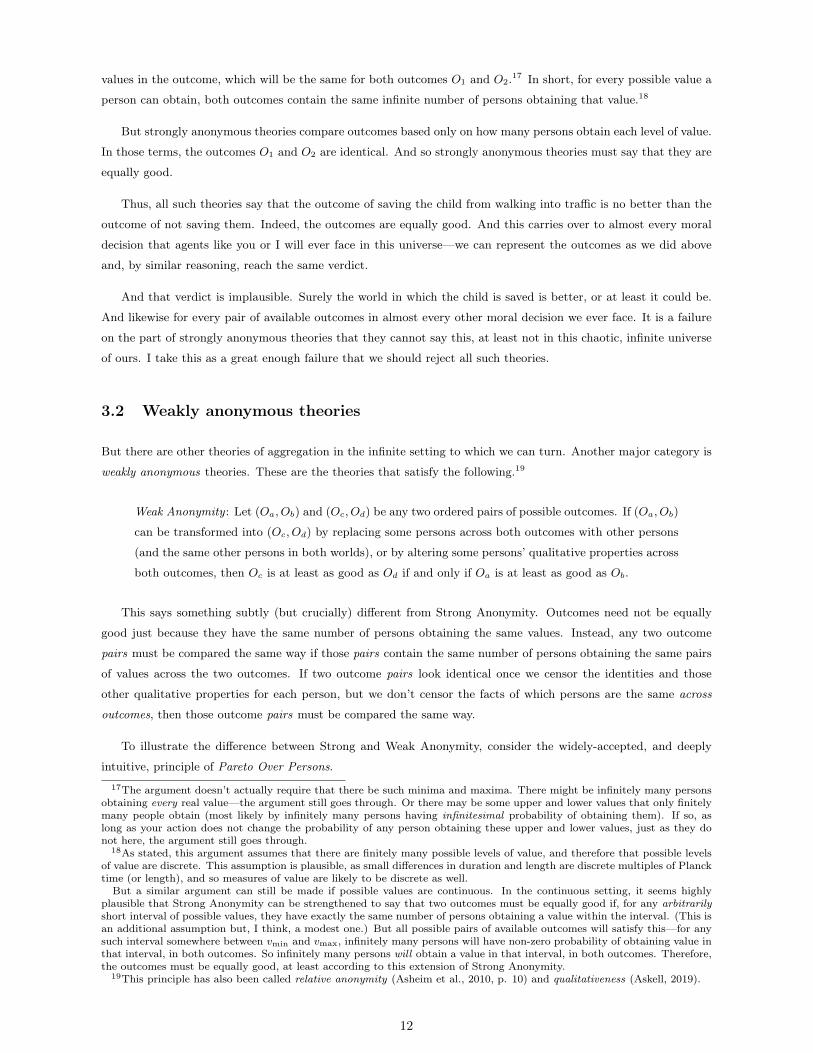
Now compare O3 to each of O2 and O1, with a slight rearrangement of how we list the persons. Both comparisons

may look familiar.

A B′ C′ D′︷ ︸︸ ︷ ︷ ︸︸ ︷ ︷ ︸︸ ︷ ︷ ︸︸ ︷pα p2 p3 p4 ... pβ pγ pδ ... p1 pi pii ... pa pb pc ...

O2 : 0 X2 X3 X4 ... Xi Xii Xiii ... 1 Xb Xc ... − − − ...

O3 : 1 X2 X3 X4 ... X ′i X ′ii X ′iii ... − − − ... 0 Xβ Xγ ...

A B′′ C′′ D′′︷ ︸︸ ︷ ︷ ︸︸ ︷ ︷ ︸︸ ︷ ︷ ︸︸ ︷pa p2 p3 p4 ... pb pc pd ... pα pβ pγ ... p1 pi pii ...

O3 : 0 X2 X3 X4 ... Xi Xii Xiii ... 1 Xb Xc ... − − − ...

O1 : 1 X2 X3 X4 ... X ′i X ′ii X ′iii ... − − − ... 0 Xβ Xγ ...

Each of these pairs is analogous to the pair (O1, O2) above. By replacing the specific identities in that pair of

outcomes (in the same way in both outcomes), we can obtain the pair (O2, O3). Likewise, we can obtain (O3, O1).

And so weakly anonymous theories must say that O1 is at least as good as O2 only if the same holds for those

other pairs. And therein lies the problem. There is no way that O2 can be better than O1, given that any plausible

‘at least as good as’ relation must be transitive (see Footnote 16). If O2 were better, we would have a cycle: O2

is better than O1, which is better than O3, which is better than O2. And similarly if O1 were better. To avoid

cycles, we must accept that either O1 and O2 are equally good or they are incomparable.

But both verdicts are implausible. Recall that these are the outcomes of saving the child from walking into

traffic and of not saving them. We cannot say that it is better to save the child. As above, that is implausible.

And so weakly anonymous theories are implausible.

Believe it or not, the problem gets even worse than this for most weakly anonymous theories. Most such theories

endorse Pareto Over Persons, as defined above. And so they should, it seems—it’s an overwhelmingly intuitive

principle and, on the face of it, a compelling reason for abandoning strongly anonymous theories for their weakly

anonymous brethren. Indeed, it is treated as axiomatic by each of the authors mentioned above. But if we accept

Pareto Over Persons, then the outcomes above cannot even be equally good; they must be incomparable. We

cannot even evaluate them!

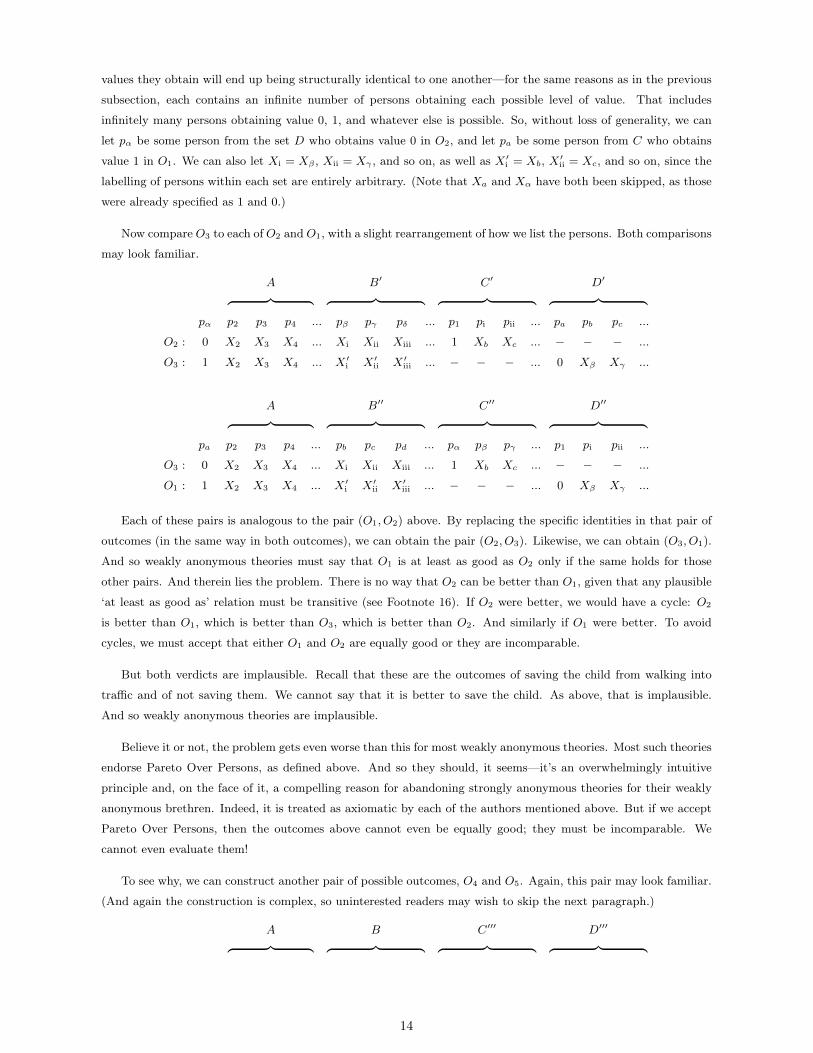
To see why, we can construct another pair of possible outcomes, O4 and O5. Again, this pair may look familiar.

(And again the construction is complex, so uninterested readers may wish to skip the next paragraph.)

A B C′′′ D′′′︷ ︸︸ ︷ ︷ ︸︸ ︷ ︷ ︸︸ ︷ ︷ ︸︸ ︷

14

p1 p2 p3 p4 ... pi′ pii′ piii′ ... pα pβ pγ ... pa pb pc ...

O4 : 0 X2 X3 X4 ... Xi Xii Xiii ... Xa Xb Xc ... − − − ...

O5 : 1 X2 X3 X4 ... X ′i X ′ii X ′iii ... − − − ... Xα Xβ Xγ ...

As before, this pair of outcomes are carefully constructed to be structurally identical to the pair (O1, O2). But

they are constructed to also ensure that each outcome is related to one of the previous outcomes by Pareto Over

Persons. This is achieved by first giving p1 the same pair of values as in (O1, O2). Then every person in A,B,C,

and D obtains the same value in O4 as in O2, and in O5 as in O1. On the same reasoning as above, we can assume

without loss of generality that Xa = Xα, Xb = Xβ , and so on for all of C and D. By similar reasoning, we also

know that B can be rearranged to the above: for every possible value between vmin and vmax, there are infinitely

many persons in B obtaining that value; but since every pair of values Xi and X ′i are independent, there will also

be infinitely many persons obtaining each pair of possible values across those two worlds; so, for any person pi who

obtains Xi and X ′i in O1 and O2 respectively, there is some pi′ who obtains X ′i and Xi respectively. And so we can

rearrange B as it has been immediately above, without changing the values obtained by any individual.

And so Pareto Over Persons compares O4 to O2 and O5 to O1. For O4 and O2, the same persons exist in both

outcomes; every person does just as well in O2 as O4 (everyone in A,B,C, and D just equally well in both), and p1

does strictly better; so Pareto implies that O2 is strictly better. Similarly, Pareto implies that O1 is strictly worse

than O5.

From above, we know that weakly anonymous views allow only that either O1 and O2 are either equally good

or they are incomparable. Suppose that they are equally good. Then, again by Weak Anonymity, O4 and O5 are

equally good. But this generates a cycle once again: O1 is equally as good as O2, which is strictly better than O4,

which is equally as good as O5, which is strictly better than O1. This is impossible, since ‘at least as good as’ is a

transitive relation. And so O1 and O2 cannot be equally good. They must instead be incomparable.22

Again, this is implausible, and even more implausible than previous implication: the disjunction that the two

outcomes are either equally good or incomparable. Surely it is better to save the child from the traffic accident

rather than not save them. And surely, at the very least, our moral theory can say something about how those

outcomes compare. But weakly anonymous theories that endorse Pareto Over Persons—all of those I have seen

seriously proposed—cannot compare them. So we should reject them, just as we did with strongly anonymous

theories.

3.3 What’s left?

We’ve ruled out both strongly anonymous and weakly anonymous theories. What’s left? In a sense, we still have

available the entire space of possible theories of aggregation that are not even weakly anonymous: those that

provide comparisons of outcomes that are at least occasionally dependent on the specific identities of the persons

in the outcome pair, or dependent on some qualitative properties of those persons beyond those mentioned above.

But many of those possible theories are clearly implausible.

Suppose we adopt a theory that admits dependency on the specific identities of the persons in the outcome

pair but not on any further qualitative properties. On such a theory, whether some outcome Oa is better than Ob

depends not just on whether it’s better for some people (de dicto); it depends on whether it’s better for specific

22This argument is adapted from Askell (2019). Askell takes arguments like this as showing that outcomes are oftenincomparable, rather than as showing that Weak Anonymity and Pareto Over Persons must be false.

15

people. For instance, some Oa may be better than Ob because it is better for Alexander, Bert, and however many

other people. But, in the qualitatively identical pair of outcomes Oa′ and Ob′ containing instead Alexandra, Beth,

and however many others, Oa′ is not better. And this is absurd.

So we are left with theories by which comparisons depend on some qualitative properties of the persons within

them (beyond just the value they obtain and whether they exist). And persons have plenty of qualitative properties

to choose from, e.g., their name, height, hair colour, ethnicity, gender, and so on. But, of course, making our moral

evaluations sensitive to changes in any of these things is counterintuitive. Doing so seems to run counter to a

basic motivation of aggregative theories: that they remain impartial in some important sense. But making our

evaluations sensitive to changes in more than one of those properties is even more counterintuitive, and an even

clearer failure of impartiality. So I will assume that, at worst, a theory of aggregation can have their comparisons

depend on just one of these further qualitative properties.

But which such property is it plausible that moral evaluations may depend on? I can see only one: position in

time and(/or) space.

Why? Suppose you have an outcome containing infinitely many persons each obtaining such and such values.

And suppose we could change some qualitative property (and only that property) of some number of those persons.

But the value each person obtains and whether they exist remain fixed. For which property is it least implausible

that those changes would mean that those two outcomes are no longer equally good?

Suppose we changed the hair colour of some (or even all) of those people. It is clearly absurd that that would

produce an outcome not equally as good as the original. Likewise for a great many properties, name, height,

ethnicity, and gender included.

But suppose instead that we changed the positions of some (or even all) of those people in space and time.

Perhaps we spread them out to be astronomically far from one another. If the original outcome has value 100 per

unit of spacetime volume, the new outcome might have just value 1 for the same volume. The universe is thereby

packed far less densely with value. It seems at least somewhat plausible that this makes the outcome worse, as a

similar reduction in value density in any universe of finite dimensions would result in a reduction in value. (The

same cannot be said of the changes in hair colour and so on, no matter how small the universe.)

And so I would suggest that the only remotely plausible theories of infinite aggregation that are neither strongly

nor weakly anonymous are those that are position-dependent : those by which comparisons of outcomes at least

sometimes depend on the positioning of persons in space and time. This is not to say, at least for now, that

these theories are anywhere near as plausible as strongly or weakly anonymous theories; they are merely the most

plausible of the remaining alternatives and, of those alternatives, the most plausible by far. So the one category of

theory I will seriously consider here is position-dependent theories.

3.4 Position-dependent theories

Some, but not all, position-dependent theories have difficulty with chaos too.

Here is one relatively simple such theory, to illustrate this difficulty: the Overtaking criterion, originally from

von Weizsäcker (1965). By this theory, we still compare outcomes by some total aggregates of value, but we don’t

represent those totals as single finite sums. Instead, we sum up the value in each outcome in the chronological order

in which that value arises. For each outcome, we take the subtotal of value up to each future time. The sequence

of such subtotals constitutes the ‘total’ of that outcome. And if one outcome has a higher subtotal than another

16

at time t, and for all future times t′, then we can say that that outcome is better. (The proposals in Vallentyne

and Kagan (1997, p. 19), Arntzenius (2014, p. 56), and Wilkinson (2021, p. 19) work in a similar way, and will

deliver the same verdicts below.) The theory can be stated precisely as follows.

Overtaking : Let Oa, Ob be any possible outcomes, and let Va(t), Vb(t) be the corresponding functions

for the value that arises at each time t ∈ R.

Then Oa is at least as good as Ob if and only if there exists t such that, for all t′ > t,

∑0≤t≤t′

(Va(t)− Vb(t)

)≥ 0

How does Overtaking fare with outcomes that differ by chaotic effects? As you might expect by now, it fares

poorly.

Consider once again the decision between not saving and saving the child from walking into traffic, with

outcomes O1 and O2 respectively. As we’ve seen, those outcomes differ by chaotic effects that continue forever.

All that distinguishes them in the agent’s eyes is that one contains that child living out the rest of their days, and

the other does not. They will also contain a lot of the same events with the same values in both outcomes. And

so too will they contain infinitely many events that differ in value in a seemingly random manner. As in Section 2,

we know that the equation that appeared in the definition of Overtaking will be equivalent to:

∑0≤t≤t′

Va(t)− Vb(t) = 1 +

n∑i=1

(Xi − Yi)

Here, the differences Xi − Yi are partially independent random variables that are all symmetric about 0. And so

this sum has the same key property as we saw in Section 2: it forms a symmetric random walk. So, as we sum it

up over time, it will again typically look like this.

1

N

1 +∑n

i=1(Xi − Yi)

Figure 4: A typical sum of 1 +∑ni=1(Xi − Yi)

As above, any such random walk will pass above and below 0 sporadically. It will never stop doing so, no

matter how large n grows (with probability arbitrarily close to 1).23 But we need the walk to stay at or above 0

from some point onwards (or else at or below 0); otherwise, Overtaking cannot say that either outcome is at least

as good as the other. For outcomes that differ this chaotically, Overtaking implies that they are incomparable.23Crucially, the walk will be recurrent : for any value it passes through, it has probability arbitrarily close to 1 of returning

to that point, indeed infinitely many times (Chung and Fuchs, 1951).

17

And so we have one of the same implausible verdicts we reached above. As we did with the previous views, we

must reject Overtaking too.24

So chaos poses just as serious a problem for some position-dependent theories; some, but thankfully not all.

There is at least one proposal that does succeed in comparing outcomes as badly behaved as O1 and O2, from

Wilkinson (2020: 30). I won’t attempt to fully defend this proposal—for my purposes here, it is enough to

demonstrate that it succeeds where others fail.

Wilkinson’s (2020) proposal is somewhat complex, but goes roughly like this: like Overtaking, we take subtotals

of the value in each world, including all value from t0 to some later (and later) time t; like Overtaking, we consider

which subtotal is greatest at each future time by taking their difference; but, unlike Overtaking, we don’t just

consider which outcome is in the lead—we also consider how often they are in the lead, and by how far. We can

obtain a useful measure of how often and by how far an outcome is in the lead over another by taking the area

under the curve (shaded below) when we graph the difference between them over time. Taking outcomes O1 and

O2, whose difference over time follows a random walk as above, that area rises sharply (as given by the black

curve).

1

1 +∑n

i=0(Xi − Yi)

n

Figure 5: A typical sum of 1 +∑ni=0(Xi − Yi), as well as the area beneath it

More formally, we can apply the following rule. Note that the sum here matches the area under the curve

above, and the limit to infinity simply makes this the limit of the area as we sum over infinite time.

Temporal Expansionism: Let Oa, Ob be any possible outcomes, and let Va(t), Vb(t) be the corresponding

functions for the value that arises at each time t. Let T = {t1, t2, ..., ti, ...} be the ordered set of all

times at which Va(ti)− Vb(ti) 6= 0, ordered from earliest to latest.

Then Oa is strictly better than Ob if the following sum diverges unconditionally to +∞.

∑tj∈T

(tj+1 − tj)( j∑i=0

(Va(ti)− Vb(ti)

))24By similar reasoning, it is straightforward to show that the proposals from Vallentyne and Kagan (1997, p. 19), Arntzenius

(2014, p. 56), and Wilkinson (2021, p. 19) reach the same implausible verdict, as they are all close relatives of Overtaking.

18

And if the sum is bounded both above and below, then Oa and Ob are equally good.2526

That sum, which corresponds to the area under the graph above, is a measure of how often and by how much

Oa’s subtotal is greater than that of Ob. If Oa’s subtotal is greater at ‘most’ times, then it will typically diverge to

+∞. Likewise, if Oa’s subtotal is greater as often as not but, when it is, it is greater by a much greater difference

than Ob’s subtotal otherwise is, then again the sum will diverge to +∞. If so, it seems plausible that Oa is better.

And if both outcomes have the greater subtotal just as often as each other, and are greater by the same amount,

then the sum will stay finite. So we might think that they are equally as good.

But how does Temporal Expansionism fare with outcomes that differ by chaotic effects? This may come as a

surprise after the failure of so many other (categories of) theories, but it does just fine.

In the graph above, note that the shaded rises sharply from the beginning, well on its way to diverging to positive

infinity. As the graph suggests, this area under the random walk does not follow the walk itself in returning to

0 over and over again. In fact, it’s guaranteed to not do so—it has probability arbitrarily close to 1 of diverging

unconditionally to either positive or negative infinity.27 And, if it diverges to +∞, then O2 is strictly better than

O1. Likewise, if it diverges to −∞, then O1 is better. So, for outcomes like these, Temporal Expansionism is

guaranteed to be able to compare them. In fact, it is guaranteed to say that one is strictly better. Good news: at

last, we have a theory that can discriminate between such outcomes.

But there is also bad news. We know that the area will diverge to +∞ or −∞, but what is the probability that

it goes to each? It is only 0.5. So, even if you adopt Temporal Expansionism, you will be radically uncertain as to

which outcome will turn out better. We cannot confidently say that it is better to save the child from the traffic

accident. As before, this is worrying—we may want our theory of aggregation to let us say confidently than one

outcome is better than another.

But this result matches the situation we faced in the finite context (see §2.4). There too it was just as likely,

approximately, that one outcome would turn out better as it was for the other. As in that setting, we are left

uncertain of which outcome is better but, since we know at least that some outcome is, the possibility is left open

that we can apply some principle of subjective, instrumental betterness to give judgements under that uncertainty.

(Readers satisfied with that resolution can skip the next section; readers who want to see just how we might apply

such a subjective betterness principle, read on.)

4 Cluelessness in infinite worlds

In practice, Temporal Expansionism lets us say that some outcome is better but it can never tell us which—we

seem to remain clueless of that fact. But is there some way that we can say that a particular action will turn

out better, perhaps along the same lines as the solution sketched in §2.4? Yes. Again we can justify that it is

subjectively better to save the child or, equivalently, that doing so produces a better lottery than the alternative.

25The original rule from Wilkinson (2021) differs in the following ways. It sums value not only over time but over expandingregions of time and space, increasing in spatial volume and temporal duration, which allows it to also compare outcomes forwhich Vi(t) is infinite for some t. And it does not assume a single absolute starting time; instead, it offers a verdict only ifthe sum diverges or is bounded for every possible starting time (and place).

26Here is a further complication: modern physics tells us that measurements of time are relative to the velocity of themeasurer. This may spell disaster for a proposal that makes moral evaluations sensitive to temporal positions. But it sohappens that we can modify the rule slightly to overcome this problem (see [omitted]).

27To see this, take any finite upper and lower bounds. It can be shown that the probability that the area under a symmetricrandom walk is within those bounds approaches 0 as r →∞ (Lipkin, 2003).

19

For my purposes, each lottery Li can be represented as a probability measure on the (minimal Boolean algebra

containing the elements of the) set of all (epistemically) possible outcomes (O). So Li maps all sets of possible

outcomes to probabilities in the interval [0,1]28, while obeying the standard probability axioms.

How should we compare lotteries? One very weak principle we can apply is Stochastic Dominance. This

principle is widely accepted in normative decision theory for finite payoffs, and also appears as an axiom for at

least one decision theory over infinite-world outcomes (see Author, n.d.). Here, O<O denotes the subset of outcomes

in O that are at least as good as outcome O.

Stochastic Dominance: Let La, Lb be any two lotteries. If Pa(O<O) ≥ Pb(O<O) for all O ∈ O, then

La is at least as good as Lb.

If as well, for some O ∈ O, Pa(O<O) − Pb(O<O) > k for some real k > 0, then La is strictly better

than Lb.29

To judge the case of saving the child or not, let L2 be the lottery over outcomes produced by saving the child,

and L1 that produced by not saving them.

It turns out that Stochastic Dominance, combined with Temporal Expansionism, judges L2 as better than

L1. To see why, take any particular outcome that could result from L2, such as O2 = (1, Yb, Yc, Yd, Ye, ...). This

outcome will be strictly better than the corresponding outcome O1 = (0, Yb, Yc, Yd, Ye, ...) that could result from

L1 (by Temporal Expansionism). And those two outcomes have precisely the same probability in their respective

lotteries. So too, the probability that L2 turns out at least as good as O2 is precisely as great as the probability

that L1 turns out at least as well as O1. And the probability that L1 turns out at least that good but worse than

O2 will be greater than 0. So we have a strictly higher probability of getting an outcome at least as good as Wsave

under L2 than we do under L1, and that holds for all such possible outcomes of Lsave. So Stochastic Dominance

implies that L2 is a better lottery than L1.

And so we can conclude that, in cases of two lotteries that each contain chaotic effects but have identical

probability distributions over those chaotic effects, the lottery that has better non-chaotic, predictable effects can

be judged the better lottery overall. We can indeed say that it is better to save the child than it is to let them

walk into traffic, even though we are clueless about exactly how either action would turn out. If we combine

a position-dependent theory with even a weak principle for comparing lotteries, we can indeed obtain plausible

practical judgements in cases like this.

Admittedly, we can only say that the outcome of saving the child is subjectively better than the alternative

(and so, plausibly, we ought to do so). We remain clueless of which outcome is objectively better—whether the the

outcome that would actually result from saving them would be better than that which results from the alternative.

But that need not trouble us. This is analogous to the situation we faced back in the finite context (Greaves, 2016),

and similar to that which we face even in much simpler finite cases (see Jackson, 1991).

28This probability measure may be real-valued, or perhaps it allows infinitesimal probabilities. I want to remain agnosticon this issue.

29Why must Pa(O<O)−Pb(O<O) be greater than some positive k, rather than just greater than 0? This makes for an evenweaker form of Stochastic Dominance than appears elsewhere. But, crucially, this change means that Stochastic Dominancewill stop short of saying that one lottery can be better than another despite having only an infinitesimally greater probabilityof O<O. It seems plausible that, if there is probability arbitrarily close to 1 that neither of two lotteries will turn out betterthan the other, neither is better. For instance, if we accept a strongly anonymous or weakly anonymous theory then, indecisions with chaotic effects, it is guaranteed (with probability arbitrarily close to 1) that no action will actually turn outbetter than any other. It seems odd to nonetheless claim that the lottery corresponding to one act is better than another.But, fortunately, the above version of Stochastic Dominance does not imply this.

20

5 Conclusion

We are often uncertain about whether our actions will turn out for better or worse. But, in a universe as chaotic

as ours, that uncertainty runs deeper than we might have thought. Actions which we might think have only trivial

effects turn out to radically and permanently change the course of the future.

That chaos poses an even greater problem given that our universe is most likely infinite. It does not merely

leave us uncertain of whether an action will turn out better than another. Thanks to chaos, we can be certain

that neither of two available actions turn out better, according to almost all aggregative theories we have at our

disposal. Even in cases where one outcome seems clearly better, they must be either equally good or incomparable.

Most aggregative theories imply this, but not quite all. Some theories still say in those cases that one outcome

is better than another. But even the most plausible such theories have a counterintuitive implication: that

comparisons of outcomes depend on the positions in space and/or time of the people within them. In any given

outcome, move sufficiently many people around and you may make the outcome better or worse. That seems a

bizarre implication for a moral theory. But, to retain remotely plausible verdicts within an aggregative theory, we

must bite this bullet. Otherwise, we must accept that the world can almost never be made better by any action,

which seems even more implausible.

You could instead draw a different conclusion from my argument. After all, one philosopher’s modus ponens

is another’s modus tollens. So too, one philosopher’s bullet to bite is another’s ammunition. You might think

it absurd that moral evaluation depends on the positioning of value in spacetime, more so than simply that all

aggregative theories are false. If so, you may take the argument above as showing that we should reject aggregation

entirely.30

ReferencesArntzenius, F., 2014. Utilitarianism, decision theory and eternity. Philosophical Perspectives, 28, 1 (2014), pp.

31–58. (cited on pages 2, 13, 17, and 18)

Asheim, G.; d’Aspremont, C.; and Banerjee, K., 2010. Generalized time-invariant overtaking. Journal ofMathematical Economics, 46, 4 (2010), pp. 519–33. (cited on page 12)

Askell, A., 2019. Pareto Principles in Infinite Ethics. PhD dissertation, New York University. (cited on pages12, 13, and 15)

Bostrom, N., 2011. Infinite ethics. Analysis and Metaphysics, 10 (2011), pp. 9–59. (cited on page 2)

Broome, J., 2004. Weighing Lives. Oxford University Press, Oxford. (cited on page 9)

Broome, J., 2019. Against denialism. The Monist, 102, 1 (2019), pp. 110–29. (cited on page 5)

Cain, J., 1995. Infinite utility. Australasian Journal of Philosophy, (1995). (cited on page 13)

Carroll, S., 2017. Why Boltzmann brains are bad. arXiv preprint, (2017). (cited on pages 1 and 2)

Chung, K. and Fuchs, W., 1951. On the distribution of values of sums of random variables. Memoirs of theAmerican Mathematical Society, 6 (1951), pp. 12. (cited on pages 7 and 17)

30Much like our future will be, this paper was shaped by the contributions of many people. I thank Jacob Schwartz, AndersSandberg, and Kyle Bogosian for their invaluable help with technical details. I thank Al Hájek, Patrick Williamson, MatthewClark, Chris Meacham, H. Orri Stefánsson, and Jasper Hedges for their extensive comments on drafts of the paper. I thankChristian Tarsney (who first prompted me to think about chaotic effects in the infinite setting), Frank Jackson, TimothyL Williamson, Adam Jonsson, Adam Elga, and seminar audiences at both the Australian National University and the 2ndOxford Workshop on Global Priorities for helpful discussion. As well, I am grateful the Forethought Foundation for GlobalPriorities Research, the Australian-American Fulbright Commission, and the Australian Research Training Program for theirfinancial support.

21

Dasgupta, P., 2008. Discounting climate change. Journal of Risk and Uncertainty, 37, 2-3 (2008), pp. 141–69.(cited on page 5)

Davenport, M. and Olum, K., 2010. Are there Boltzmann brains in the vacuum? arXiv preprint, (2010). (citedon page 2)

Dreier, J., 2019. World-centered value. In Consequentialism: New Directions and Problems (Ed. C. Seidel), p.31–50. Oxford University Press, Oxford. (cited on page 9)

Feldman, D., 2019. Chaos and Dynamical Systems. Princeton University Press, Princeton. (cited on page 3)

Garriga, J. and Vilenkin, A., 2001. Many worlds in one. Physical Review D, 64, 4 (2001), 043511. (cited onpage 1)

Gleick, J., 1987. Chaos: Making a New Science. Viking Books, New York. (cited on page 3)

Greaves, H., 2016. Cluelessness. Proceedings of the Aristotelian Society, 116, 3 (2016), pp. 311–39. (cited onpages 1, 4, 6, and 20)

Grimmett, G. and Stirzaker, D., 1992. Probability and Random Processes. Clarendon Press, Oxford. (citedon page 4)

Huemer, M., 2008. In defence of repugnance. Mind, 117, 468 (2008), pp. 899–933. (cited on page 9)

Jackson, F., 1991. Decision-theoretic consequentialism and the nearest and dearest objection. Ethics, 101, 3(1991), pp. 461–82. (cited on pages 8 and 20)

Laskar, J., 1989. A numerical experiment on the chaotic behavior of the solar system. Nature, 338, 6212 (1989),pp. 237–8. (cited on page 6)

Lauwers, L. and Vallentyne, P., 2004. Infinite utilitarianism: more is always better. Economics & Philosophy,20, 2 (2004), pp. 307–30. (cited on pages 2 and 13)

Lenman, J., 2000. Consequentialism and cluelessness. Philosophy and Public Affairs, 29, 4 (2000), pp. 342–70.(cited on page 6)

Lighthill, M. and Whitham, G., 1955. On kinematic waves ii: A theory of traffic flow on long crowded roads.Proceedings of the Royal Society of London. Series A. Mathematical and Physical Sciences, 229, 1178 (1955), pp.317–45. (cited on page 1)

Lipkin, L., 2003. Tossing a fair coin. The College Mathematics Journal, 34, 2 (2003), pp. 128–33. (cited on page19)

Lorenz, E., 1963. Deterministic nonperiodic flow. Journal of the Atmospheric Sciences, 20, 2 (1963), pp. 130–41.(cited on page 5)

Lorenz, E., 1972. Does the flap of a butterfly’s wings in Brazil set off a tornado in Texas? (1972). (cited onpage 5)

MacAskill, W. and Mogensen, A., 2021. The paralysis argument. Philosophers’ Imprint, 21 (2021). (citedon page 1)

Malhotra, R.; Holman, M.; and Ito, T., 2001. Chaos and stability of the solar system. Proceedings of theNational Academy of Sciences, 98, 22 (2001), 12342–3. (cited on page 5)

Melchers, M.; Montag, C.; Reuter, M.; Spinath, F.; and Hahn, E., 2016. How heritable is empathy?differential effects of measurement and subcomponents. Motivation and Emotion, 40, 5 (2016), pp. 720–30.(cited on page 4)

Nebel, J., 2018. The good, the bad, and the transitivity of better than. Noûs, 52, 4 (2018), pp. 874–99. (cited onpage 9)

Office for National Statistics, 2018. Childbearing for women born in different years, Eng-land and Wales: 2017. https://www.ons.gov.uk/peoplepopulationandcommunity/birthsdeathsandmarriages/conceptionandfertilityrates/bulletins/childbearingforwomenbornindifferentyearsenglandandwales/2017. (ac-cessed: 02.09.2020). (cited on page 4)

Office for National Statistics, 2019. National life tables: UK. https://www.ons.gov.uk/peoplepopulationandcommunity/birthsdeathsandmarriages/lifeexpectancies/datasets/nationallifetablesunitedkingdomreferencetables. (accessed: 02.09.2020). (cited on page 4)

22

Palmer, T.; Döring, A.; and Seregin, G., 2014. The real butterfly effect. Nonlinearity, 27, 9 (2014), R123.(cited on page 5)

Parfit, D., 1984. Reasons and Persons. Oxford University Press, Oxford. (cited on page 4)

Pemantle, R., 2007. A survey of random processes with reinforcement. Probability Surveys, 4 (2007), pp. 1–79.(cited on page 8)

Plomin, R. and Deary, I. J., 2015. Genetics and intelligence differences: five special findings. MolecularPsychiatry, 20, 1 (2015), 98–108. (cited on page 4)

Poincaré, H., 1890. The Three-Body Problem and the Equations of Dynamics: Poincaré’s Foundational Work onDynamical Systems Theory. Popp, Bruce D. (trans.), Springer International Publishing (2017). (cited on page5)

Putensen, C. and Wrigge, H., 2007. Tidal volumes in patients with normal lungs: one for all or the less, thebetter? Anesthesiology, 106 (2007), pp. 1085–7. (cited on page 5)

Railton, P., 1984. Alienation, consequentialism, and the demands of morality. Philosophy and Public Affairs, 13(1984). (cited on page 9)

Tang, J.; Nicolle, A.; Klettner, C. A.; Pantelic, J.; Wang, L.; and Tan, A. B. S. A., 2013. Airflowdynamics of human jets: sneezing and breathing - potential sources of infectious aerosols. PLOS ONE, 8, 4(2013), e59970. (cited on page 5)

Vallentyne, P., 1993. Utilitarianism and infinite utility. Australasian Journal of Philosophy, 71, 2 (1993), pp.212–7. (cited on page 2)

Vallentyne, P. and Kagan, S., 1997. Infinite value and finitely additive value theory. Journal of Philosophy,94, 1 (1997), pp. 5–26. (cited on pages 2, 13, 17, and 18)

van Liedekerke, L., 1995. Should utilitarians be cautious about an infinite future? Australasian Journal ofPhilosophy, 73, 3 (1995), pp. 405–7. (cited on pages 10 and 13)

von Weizsäcker, C., 1965. Existence of optimal programs of accumulation for an infinite time horizon. TheReview of Economic Studies, 32, 2 (1965), pp. 85–104. (cited on page 16)

Wainschtein, P.; Jain, D. P.; Yengo, L.; Zheng, Z.; Cupples, L. A.; Shadyab, A. H.; and McKnight,B., 2019. Recovery of trait heritability from whole genome sequence data. BioRxiv, (2019), 588020. (cited onpage 4)

Wald, R., 1983. Asymptotic behavior of homogeneous cosmological models in the presence of a positive cosmo-logical constant. Physical Review D, 28, 8 (1983), pp. 2118. (cited on page 1)

Wilkinson, H., 2021. Infinite aggregation: Expanded addition. Philosophical Studies, 178, 6 (2021), pp. 1917–49.(cited on pages 2, 13, 17, 18, and 19)

23