Global Well-Posedness of an Inviscid Three-Dimensional Pseudo-Hasegawa-Mima Model
Upload
khangminh22Category
view
1download
0
WELL-POSEDNESS IN ENERGY SPACE FOR THE PERIODICMODIFIED BENJAMIN-ONO EQUATION
ZIHUA GUO1,2, YIQUAN LIN1,2, LUC MOLINET3
Abstract. We prove that the periodic modified Benjamin-Ono equation is locallywell-posed in the energy space H1/2. This ensures the global well-posedness in thedefocusing case. The proof is based on an Xs,b analysis of the system after gaugetransform.
Contents
1. Introduction, main results and notations 11.1. Notations 42. Gauge transform 53. The main estimates and proof of Theorem 1.1 73.1. Linear Estimates 73.2. Main Non-linear Estimates 83.3. Proof of Proposition 3.2 93.4. Proof of Theorem 1.1 114. Proof of the estimates on v 124.1. Estimate on G(u) 124.2. Estimates on suitable extensions of u and e−iF (u) . 134.3. Multilinear estimates 15Acknowledgment 25References 25
1. Introduction, main results and notations
In this paper, we study the Cauchy problem for the modified Benjamin-Ono equa-tion on the torus that reads {
∂tu+H∂2xu = ∓u2ux,
u(x, 0) = u0
(1.1)
where u(t, x) : R× T→ R, T = R/2πZ and H is the Hilbert transform
Hf(0) = 0, Hf(k) = −isgn(k)f(k), k ∈ Z∗.
This equation is called defocusing when there is a minus sign in front of the nonlinearterm u2ux and focusing when it is a plus sign.The Benjamin-Ono equation with the quadratic nonlinear term
∂tu+H∂2xu =uux (1.2)
1
2 Z. GUO, Y. LIN, L. MOLINET
was derived by Benjamin [2] and Ono [25] as a model for one-dimensional waves indeep water. On the other hand, the cubic nonlinearity is also of much interest forlong wave models [1, 13].
There are at least the three following quantities preserved under the flow of thereal-valued mBO equation (1.1)1∫
Tu(t, x)dx =
∫Tu0(x)dx, (1.3)∫
Tu(t, x)2dx =
∫Tu0(x)2dx, (1.4)∫
T
1
2uHux ∓
1
12|u(t, x)|4dx =
∫T
1
2u0Hu0,x ∓
1
12|u0(x)|4dx . (1.5)
These conservation laws provide a priori bounds on the solution. For instance, inthe defocusing case we get from (1.4) and (1.5) that the H1/2 norm of the solutionremains bounded for all times if the initial data belongs to H1/2. This is crucial inorder to prove the well-posedness result. On the other hand the mBO equation isL2-critical (in the sense that the L2(R)-norm is preserved by the dilation symmetryof the equation). Therefore, in the focusing case, one expects that a phenomenon ofblow-up in the energy space occurs2
The Cauchy problems for (1.1) and the Benjamin-Ono equation (1.2) have beenextensively studied. For instance, in both real-line and periodic case, the energymethod provides local well-posedness for BO and mBO in Hs for s > 3/2 [10]. Inthe real-line case, this result was improved by combination of energy method and thedispersive effects. For real-line BO equation, the result s ≥ 3/2 by Ponce [26] wasthe first place of such combination as a consequence of the commutator estimates in[11], was later improved to s > 5/4 in [17], and s > 9/8 in [12]. Tao [27] obtainedglobal well-posedness in Hs for s ≥ 1 by using a gauge transformation as for thederivative Schrodinger equation and Strichartz estimates. This result was improvedto s ≥ 0 by Ionescu and Kenig [9], and to s ≥ 1/4 (local well-posedness) by Burqand Planchon [4]. Their proof both used the Fourier restriction norm introduced in[3]. Recently, Molinet and Pilod [18] gave a simplified proof for s ≥ 0 and obtainedunconditional uniqueness for s > 1/4.
For the real-line mBO, this was improved to s ≥ 1 by Kenig-Koenig [12] by theenhanced energy methods. Molinet and Ribaud [20] obtained analytic local well-
posedness for the complex-valued mBO in Hs for s > 1/2 and B1/22,1 with a small
L2 norm, improving the result of Kenig-Ponce-Vega [14] for s > 1. The smallnesscondition of Hs(s > 1/2) results was later removed in [19] by using Tao’s gaugetransformation [27]. The result for s = 1/2 was obtained by Kenig and Takaoka[15] by using frequency dyadically localized gauge transformation. Their result issharp in the sense that the solution map is not locally uniformly continuous in Hs fors < 1/2 (The failure of C3 smoothness was obtained in [20]). Later, Guo [7] obtainedthe same result without using gauge transform under a smallness condition on theL2 norm.
1In (1.5) the + corresponds to the defocusing case whereas the − corresponds the the focusingone.
2Progress in this direction can be found in [16] for the case on the real line.

PERIODIC MBO EQUATION 3
In the periodic case, there is no smoothing effect for the equation. However, toovercome the loss of derivative, the gauge transform still applies. For the periodicBO equation, global well-posedness in H1 was proved by Molinet and Ribaud [23],was later improved by Molinet to H1/2 [22], and L2 [21]. Molinet [24] also provedthat the result in L2 is sharp in the sense that the solution map fails to be continuousbelow L2. For the periodic mBO (1.1), local well-posedness in H1 was proved in[23]. Their proof used the Strichartz norm and gauge transform.
The purpose of this paper is to improve the well-posedness results for (1.1) to theenergy space H1/2 and, as a by-product, to prove that the solutions can be extendedfor all times in the defocusing case. The main result of this paper is
Theorem 1.1. Let s ≥ 1/2. For any intial data u0 ∈ Hs(T) there exists T =T (‖u0‖H1/2) > 0 such that the mBO equation (1.1) admits a unique solution
u ∈ C([−T, T ];Hs(T)) with P+(eiF (u)) ∈ X12, 12
T .
Moreover, the solution-map u0 7→ u is continuous from the ball of H1/2(T) of radius‖u0‖H1/2, equipped with the Hs(T)-topology, with values in C([−T, T ];Hs(T)).Finally, in the defocusing case, the solution can be extended for all times and belongsto C(R;Hs(T)) ∩ Cb(R;H1/2(T)).
A very similar equation to mBO (1.1) is the derivative nonlinear Schrodingerequation {
i∂tu+ ∂2xu = i(|u|2u)x, (t, x) ∈ R× T
u(0, x) = u0.(1.6)
It has also attracted extensive attention. Local well-posedness for (1.6) in H1/2 wasproved by Herr [8]. There are several differences between (1.1) and (1.6). The firstone is the integrability: (1.6) is integrable while (1.1) is not. The second one is theconservation laws: (1.1) has a conservation law at level H1/2, and hence GWP inH1/2 is much easier. The last one is the action of the gauge transform: let v bethe function after gauge transform, (1.6) can be reduced to a clean equation whichinvolves only v, while (1.1) can only reduce to a system that involves both u and v,and hence the gauge for (1.1) brings more technical difficulties.
We discuss now the ingredients in the proof of Theorem 1.1. Let u be a smoothsolution to (1.1), define
w = T (u) :=1√2u(t, x−
∫ t
0
1
2π
∫u2(s, x)dxds). (1.7)
Then w solves the ”Wicked order” mBO equation:{∂tu+H∂2
xu = 2P 6=c(u2)ux,
u(x, 0) = u0,(1.8)
where P 6=cf = f − 12π
∫T fdx. It is easy to see that T and its inverse T−1 are both
continuous maps from C((−T, T ) : Hs) to C((−T, T ) : Hs) for s ≥ 0. Therefore wewill consider (1.8) instead of (1.1). Now, in order to overcome the loss of derivative,we will apply the method of gauge transform as in [23, 21, 22], which was firstdeveloped for BO equation by Tao [27]. As noticed above the equation satisfied
4 Z. GUO, Y. LIN, L. MOLINET
by this gauge transform v involves terms with both u and v. One of the maindifficulties is that the solution u does not share the same regularity in Bourgain’spaceas the gauge transform v. The main new ingredient is the use of the Marcinkiewiczmultiplier theorem that enables us to treat the multiplication by u in Bourgain’spacein a simple way.
1.1. Notations. For A,B > 0, A . B means that there exists c > 0 such thatA ≤ cB. When c is a small constant we use A� B. We write A ∼ B to denote thestatement that A . B . A.
We denote the sum on Z by integral form∫a(ξ)dξ :=
∑ξ∈Z a(ξ). For a 2π-periodic
function φ, we define its Fourier transform on Z by
φ(ξ) :=
∫R/2πZ
e−iξxφ(x)dx, ∀ ξ ∈ Z.
We denote by W (·) the unitary group W (t)u0 := F−1x e−it|ξ|ξFxu0(ξ).
For a function u(t, x) on R×R/(2π)Z, we define its space-time Fourier transformas follows, ∀ (τ, ξ) ∈ R× Z
u(τ, ξ) := Ft,x(u)(τ, ξ) := F(u)(τ, ξ) =
∫R
∫R/(2π)Z
e−i(τt+ξx)u(t, x)dxdt.
Then define the Sobolev spaces Hs for (2π)-periodic function by
‖φ‖Hs := ‖〈ξ〉sφ‖l2ξ = ‖Jsxφ(x)‖L2x,
where 〈ξ〉 := (1 + |ξ|2)12 and Jsxφ(ξ) := 〈ξ〉sφ(ξ). For 2 < q < ∞ we define also the
Sobolev type spaces Hsq by
‖φ‖Hsq
:= ‖Jxs φ‖Lq .We will use the following Bourgain-type spaces denoted by Xs,b, Zs,b and Y s of(2π)-periodic (in x) functions respectively endowed with the norm
‖u‖Xs,b :=‖〈ξ〉s〈τ + |ξ|ξ〉bu(τ, ξ)‖L2τ,ξ,
‖u‖Zs,b :=‖〈ξ〉s〈τ + |ξ|ξ〉bu(τ, ξ)‖L2ξL
1τ,
and
‖u‖Y s := ‖u‖Xs, 12
+ ‖u‖Zs,0 . (1.9)
One can easily check that u 7→ u an isometry in Xs,b and Zs,b and that Y s ↪→Zs,0 ↪→ C(R;Hs). We will also use the space-time Lebesgue spaces denoted byLptL
qx of (2π)-periodic (in x) functions endowed with the norm
‖u‖LptLqx :=(∫
R‖u(t, ·)‖p
Lqxdt)1/p
,
with the obvious modification for p =∞. For any space-time function space B andany T > 0, we denote by BT the corresponding restriction in time space endowedwith the norm
‖u‖BT := infv∈B{‖v‖B, v(·) ≡ u(·) on (0, T )}.
Let η0 : R → [0, 1] denote an even smooth function supported in [−8/5, 8/5]and equal to 1 in [−5/4, 5/4]. For k ∈ N∗ let χk(ξ) = η0(ξ/2k−1) − η0(ξ/2k−2),

PERIODIC MBO EQUATION 5
η≤k = η0(ξ/2k−1), and then let P2k and P≤2k denote the operators on L2(T) definedby
P1u(ξ) = η0(2ξ), P2ku(ξ) = χk(ξ)u(ξ) , k ∈ N∗, and P≤2ku(ξ) = η≤k(ξ)u(ξ) .
By a slight abuse of notation we define the operators P2k , P≤2k on L2(R × T) bythe formulas F(P2ku)(τ, ξ) = χk(ξ)F(u)(τ, ξ), F(P≤2ku)(τ, ξ) = η≤k(ξ)F(u)(τ, ξ).We also define the projection operators P±f = F−11±ξ>0Ff , Pcf = 1
2π
∫T fdx,
P 6=c = I − Pc, and P+2k
= P+P2k , P+≤2k
= P+P≤2k .To simplify the notation, we use capitalized variables to describes the dyadic
number, i.e. any capitalized variables such as N range over the dyadic number 2N.Finally, for any 1 ≤ p ≤ ∞ and any function space B we define the space-time
function space LptB by
‖u‖gLptB :=( ∞∑k=0
‖P2ku‖2LptB
) 12.
It is worth noticing that Littlewood-Paley square function theorem ensures that
LptLpx ↪→ LptL
px for 2 ≤ p <∞.
2. Gauge transform
In this section, we introduce the gauge transform. Let u ∈ C([−T, T ] : H∞(T))be a smooth solution to (1.8). Define the periodic primitive of u2 − 1
2π‖u(t)‖2
2 withzero mean by
F = F (u) = ∂−1x P 6=c(u
2) =1
2π
∫ 2π
0
∫ x
θ
u2(t, y)− 1
2π‖u(t)‖2
L2dydθ.
Let
v = G(u) := P+(e−iFu), (2.1)
then we look for the equation that v solves. It holds
vt =P+[e−iF (−iFtu+ ut)],
vxx =P+[e−iF (−F 2xu− iFxux − i(Fxu)x + uxx)] ,
and thus
vt − ivxx =P+[e−iF (−iFtu+ i(Fx)2u− Fxxu)]
+ P+[e−iF (ut − iuxx − 2Fxux)] := I + II.
Using equation (1.8) we easily get
II =P+[e−iF (ut +Huxx − 2iP−uxx − 2Fxux)] = −2iP+[e−iFP−uxx].

6 Z. GUO, Y. LIN, L. MOLINET
Next we compute I. Using again (1.8) and the conservation of the L2-norm forsmooth solutions, we have
Ft =∂t∂−1x (P 6=cu
2) = ∂−1x ∂t(u
2 − Pcu2) = ∂−1x ∂tu
2
=2∂−1x
(−uHuxx + 2P 6=c?u
2)uux
)=2∂−1
x
(−∂x(uHux) + uxHux + P 6=c(u
2)∂xP 6=c(u2))
=P 6=c
((P 6=cu
2)2)− 2uHux + 2Pc?uHux) + 2∂−1
x (uxHux) . (2.2)
Noticing that Fx = P 6=c(u2) we infer that
−iuP 6=c(
(P 6=cu2)2)
+ iu(Fx)2 = iuPc
((P 6=cu
2)2)
and noticing that Fxx = 2uux,
2iuP 6=c
(uH∂xu
)− Fxxu = −4u2P−ux?2iuPc(uHux) .
Moreover, following [19], we will use the symmetry of the term ∂−1x (uxHux). Indeed,
it is easy to check that ∂−1x (uxHux) = −i∂−1
x (P+ux)2 + i∂−1
x (P−ux)2 and thus setting
B(u, v) = −i∂−1x (P+uxP+vx) + i∂−1
x (P−uxP−vx) , (2.3)
we infer that ∂−1x (uxHux) = B(u, u). We thus finally get
I = P+
[e−iF
(−4u2P−ux − 2iuB(u, u) + 2iuPc(uHux)− iuPc
((P 6=cu
2)2)]
which leads to
vt − ivxx =P+
[e−iF
(−4u2P−ux − 2iP−uxx − 2iuB(u, u)
− 2iuPc(uHux) + iuPc
((P 6=cu
2)2))]
. (2.4)
Due to the projector P+, P−, we see formally that in the system (2.1)-(2.4) there isno high-low interaction of the form
Plowu2 · ∂xPhighu.
Note that u→ G(u) can be ”inverted” in Lebesgue space. This is the strategy usedin [23] to prove well-posedness in H1. To go below to H1/2, we intend to use Xs,b
spaces. But u→ G(u) can not be well ”inverted” in Bourgain’spaces and thus u willnot have the same regularity as G(u) in these spaces. To handle this former difficulty,we will insert the ”inverse” into some of the terms in (2.4). We first observe that
−2iP+
(e−iFP−uxx
)=− 2i∂xP+(e−iFP−ux) + 2P+(e−iFP 6=c(u
2)P−ux)
=− 2∂xP+(∂−1x P+(e−iFP 6=c(u
2))P−ux)
+ 2P+(e−iFu2P−ux)− 2Pc(u2)P+(e−iFP−ux)
and thus the sum of the first two terms of the right-hand side of (2.4) can berewritten as
− 2P+(e−iFu2P−ux)− 2∂xP+(∂−1x P+(e−iFu2)P−ux)
+ 2Pc(u2)(∂xP+(∂−1
x P+e−iFP−ux)− P+(e−iFP−ux)
). (2.5)
PERIODIC MBO EQUATION 7
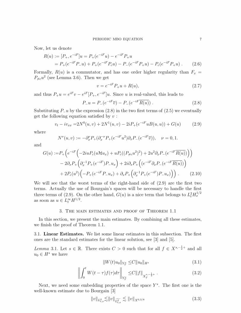
Now, let us denote
R(u) := [P+, e−iF ]u = P+(e−iFu)− e−iFP+u
= P+(e−iFP−u) + P+(e−iFPcu)− P−(e−iFP+u)− Pc(e−iFP+u) . (2.6)
Formally, R(u) is a commutator, and has one order higher regularity than Fx =P 6=cu
2 (see Lemma 3.6). Then we get
v = e−iFP+u+R(u), (2.7)
and thus P+u = eiFv − eiF [P+, e−iF ]u. Since u is real-valued, this leads to
P−u = P−(e−iFv)− P−(e−iFR(u)) . (2.8)
Substituting P−u by the expression (2.8) in the two first terms of (2.5) we eventuallyget the following equation satisfied by v :
vt − ivxx =2N0(u, v) + 2N1(u, v)− 2iP+(e−iFuB(u, u)) +G(u) (2.9)
where
N ν(u, v) := −∂νxP+(∂−νx P+(e−iFu2)∂xP−(e−iFv)), ν = 0, 1.
and
G(u) :=P+
(e−iF
(−2iuPc(uHux) + uPc((P 6=cu
2)2) + 2u2∂xP−(e−iFR(u))))
− 2∂xP+
(∂−1x P+(e−iF )P−ux
)+ 2i∂xP+
((e−iF∂xP−(e−iFR(u))
)+ 2Pc(u
2)(−P+(e−iFP−ux) + ∂xP+
(∂−1x P+(e−iF )P−ux)
)). (2.10)
We will see that the worst terms of the right-hand side of (2.9) are the first twoterms. Actually the use of Bourgain’s spaces will be necessary to handle the first
three terms of (2.9). On the other hand, G(u) is a nice term that belongs to L2tH
1/2x
as soon as u ∈ L∞t H1/2.
3. The main estimates and proof of Theorem 1.1
In this section, we present the main estimates. By combining all these estimates,we finish the proof of Theorem 1.1.
3.1. Linear Estimates. We list some linear estimates in this subsection. The firstones are the standard estimates for the linear solution, see [3] and [5].
Lemma 3.1. Let s ∈ R. There exists C > 0 such that for all f ∈ Xs,− 12
+ and allu0 ∈ Hs we have
‖W (t)u0‖Y sT ≤C‖u0‖Hs (3.1)∥∥∥∥∫ t
0
W (t− τ)f(τ)dτ
∥∥∥∥Y sT
≤C‖f‖Xs,− 1
2+
T
. (3.2)
Next, we need some embedding properties of the space Y s. The first one is thewell-known estimate due to Bourgain [3]
‖v‖L4t,x.‖v‖gL4
t,x. ‖v‖X0,3/8 (3.3)

8 Z. GUO, Y. LIN, L. MOLINET
where the first inequality above follows from the Littlewood-Paley square functiontheorem. Note that (3.1) combined with (3.3) ensures that for 0 ≤ T ≤ 1,
‖W (t)u0‖L4tx. ‖u0‖L2 . (3.4)
3.2. Main Non-linear Estimates.
Proposition 3.2 (Estimates of u). Let T ∈]0, 1[, s ∈ [12, 1] and (ui, vi) ∈
(C0TH
s ∩
L4TH
s4
)× Y s
T , i = 1, 2, satisfying (1.8) and (2.1) on ] − T, T [ with initial data ui,0.
Then for u = ui
‖u‖L4TH
s4
. (1 + ‖u‖4
L∞T H12)‖v‖Y sT + T
14 (1 + ‖u‖8
L∞T H12)‖u‖
L∞T H12, (3.5)
and for large N ∈ N, we have
‖u‖L∞T Hs.‖u0‖Hs + TN2‖u‖3L∞T H
1/2 + ‖v‖Y sT+N−
14 (‖u‖
L∞T H12
+ ‖v‖Y sT )(1 + ‖u‖8
L∞T H12). (3.6)
Moreover, we have
‖u1 − u2‖ ˜L4TH
1/24
.(1 + ‖u‖4L∞T H
1/2)‖v1 − v2‖Y
12T
+ ‖u1 − u2‖L∞T H1/2‖v1‖Y
12T
2∏i=1
(1 + ‖ui‖L∞T H12)3
+ T 1/4‖u1 − u2‖L∞T H12
2∏i=1
(1 + ‖ui‖L∞T H12)8 (3.7)
and
‖u1 − u2‖L∞T H1/2.‖u1,0 − u2,0‖H1/2 +2∏i=1
(1 + ‖ui‖L∞T H12
+ ‖vi‖Y 1/2T
)8
×(‖v1 − v2‖Y 1/2
T+ (TN2 +N−1/4)‖u1 − u2‖L∞T H
12
). (3.8)
Proposition 3.3 (Estimates of v). Let 0 < T < 1, s ∈ [12, 1] and (ui, vi) ∈
(C0tH
s ∩
L4TH
s4
)× Y s
T satisfying (1.8), (2.1) and (2.9) on ]− T, T [. Then for (u, v) = (ui, vi)
there exists ν > 0 and q ∈ N∗ such that
‖v‖Y sT.(1 + ‖u0‖4
H12)‖u0‖Hs + T ν
((1 + ‖u‖q+1
L∞T H12∩L4H
1/24
)‖v‖Xs,1/2
+ (1 + ‖u‖qL∞T H
12∩L4H
1/24
)‖v‖X1/2,1/2‖u‖L∞T H
s∩L4Hs4
). (3.9)

PERIODIC MBO EQUATION 9
and
‖v1 − v2‖Y
12T
.(1 + ‖u0‖4
H12)‖u1,0 − u2,0‖Hs (3.10)
+ T ν[(
1 +2∑i=1
‖ui‖q+1
L∞T H12 ∩L4H
1/24
)‖v1 − v2‖Xs,1/2
+(
1 +2∑i=1
‖ui‖qL∞T H
12∩L4H
1/24
)(
2∑i=1
‖vi‖X1/2,1/2)‖u1 − u2‖L∞T Hs∩L4Hs4
].
(3.11)
The rest of this subsection is devoted to proving Proposition 3.2, while the proofof Proposition 3.3 will be given in the next section.
3.3. Proof of Proposition 3.2. We start with recalling some technical lemmasthat will be needed hereafter. We first recall the Sobolev multiplication laws.
Lemma 3.4. (a) Assume one of the following condition
s1 + s2 ≥ 0, s ≤ s1, s2, s < s1 + s2 −1
2,
or s1 + s2 > 0, s < s1, s2, s ≤ s1 + s2 −1
2.
Then‖fg‖Hs.‖f‖Hs1‖g‖Hs2 .
(b) For any s ≥ 0, we have
‖fg‖Hs.‖f‖Hs‖g‖L∞ + ‖g‖Hs‖f‖L∞ .
Second, we state the classical fractional Leibniz rule estimate derived by Kenig,Ponce and Vega (See Theorems A.8 and A.12 in [14]).
Lemma 3.5. Let 0 < α < 1, p, p1, p2 ∈ (1,+∞) with 1p1
+ 1p2
= 1p
and α1, α2 ∈ [0, α]
with α = α1 + α2. Then,∥∥Dαx (fg)− fDα
xg − gDαxf∥∥Lp. ‖Dα1
x g‖Lp1‖Dα2x f‖Lp2 . (3.12)
Moreover, for α1 = 0, the value p1 = +∞ is allowed.
The next estimate is a frequency localized version of estimate (3.12) in the samespirit as Lemma 3.2 in [27]. It allows to share most of the fractional derivative inthe first term on the right-hand side of (3.13).
Lemma 3.6. Let α, β ≥ 0 and 1 < q <∞. Then,∥∥DαxP∓
(fP±D
βxg)∥∥
Lq. ‖Dα1
x f‖Lq1‖Dα2x g‖Lq2 , (3.13)
with 1 < qi <∞, 1q1
+ 1q2
= 1q
and α1 ≥ α, α2 ≥ 0 and α1 + α2 = α + β.
Proof. See Lemma 3.2 in [21]. �
Finally we state the two following lemmas. The first one is a direct consequence of
the continuous embeddings Hs+1/4 ↪→ H1/24 ↪→ L∞ whereas the proof of the second
one (in the real line case) can be found in [[19], Lemma 6.1].

10 Z. GUO, Y. LIN, L. MOLINET
Lemma 3.7. Let s ∈ [1/2, 1], z ∈ L∞T Hs+ 14 and v ∈ L4
THs4 then
‖zv‖L4TH
s4
. ‖z‖L∞T H
s+14+‖v‖L4
THs4
(3.14)
Lemma 3.8. Let v1, v2 ∈ L4H1/24 then
‖B(v1, v2)‖L2 . ‖D1/2x v1‖L4‖D1/2
x v2‖L4 (3.15)
Let k ∈ Z∗ with |k| ≤ 10. A direct computation gives
∂x(eikF ) = kieikF (u2 − Pc(u2)), (3.16)
Next by gathering the obvious estimates ‖eikF‖L∞T L2x.1 and ‖∂x(eikF )‖L∞T L2
x.Pc(u2)+
‖u‖2L∞T L
4x, we get
‖eikF‖L∞T H1.1 + ‖u‖2
L∞T H12. (3.17)
On the other hand, by Lemma 3.4, we have for any s ∈ [1/2, 1],
‖∂x(eikF )‖L∞T Hs−.‖eikF‖L∞T H1‖u2 − Pc(u2)‖L∞T Hs−.(1 + ‖u‖2
L∞T H12)‖u‖
L∞T H12‖u‖L∞T Hs .
Gathering the above estimates leads for any s ∈ [1/2, 1] to
‖eikF‖L∞T Hs+1−.(1 + ‖u‖2
L∞T H12)(
1 + ‖u‖L∞T H
12‖u‖L∞T Hs
)(3.18)
and, in view of (2.6) and Lemma 3.6, it holds
‖R(u)‖L∞T H
54+ . ‖eiF‖
L∞T H54+
2+
‖u‖L∞T L∞−x (3.19)
. ‖e−iF‖L∞T H
32−‖u‖
L∞T H12
. (1 + ‖u‖4
L∞T H12)‖u‖
L∞T H12. (3.20)
Now, for s ∈ [1/2, 1], according to (2.7), (3.18)-(3.20) and Lemma 3.7?we easily get
‖P+u‖L4TH
s4
. ‖eiFv‖L4TH
s4
+ ‖eiFR(u)‖L4TH
s4
. ‖eiF‖L∞t H3/2−‖v‖L4TH
s4
+ T14‖eiF‖L∞t H3/2−‖R(u)‖
L∞t H54+
. (1 + ‖u‖4
L∞T H12)(‖v‖Y sT + T
14 (1 + ‖u‖4
L∞T H12)‖u‖
L∞T H12
)Estimate (3.5) follows by using that u is real valued and the conservation of themean-value by (1.8).Next, in order to get a better estimate of ‖u‖L∞T Hs , s ∈ [1
2, 1], we split u into a low
frequency and a high frequency part. For low frequency, we use the equation for u,while for high frequency, we use P+u = eiFv − eiFR(u). For any N = 2k ∈ N, ands ∈ [1
2, 1], we have
‖u‖L∞T Hs . ‖P≤ku‖L∞T Hs + 2‖P+≥ku‖L∞T Hs .
By the equation of u, we have
P≤ku = W (t)P≤ku0 +1
3
∫ t
0
W (t− τ)P≤k∂x(u3)(τ)dτ,

PERIODIC MBO EQUATION 11
that leads to
‖P≤ku‖L∞T Hs.‖u0‖Hs + T22k‖u‖3L∞T H
1/2 .
To estimate the term ‖P+≥ku‖L∞T Hs , we use P+u = eiFv − eiFR(u). By (3.17)
-(3.20) we have
‖P+≥k[e
iFR(u)]‖L∞T Hs . N−1/4‖e−iFR(u)‖L∞T H5/4
. N−14 (1 + ‖u‖8
L∞T H12)‖u‖L∞T H1/2 .
It remains to estimate ‖P+≥k[e
iFv]‖Hs . By Lemma 3.4 we have
‖P+≥k[e
iFv]‖L∞t Hs.‖P+≥k[P≤k−5(eiF )v]‖L∞t Hs + ‖P+
≥k[P>k−5(eiF )v]‖L∞t Hs
.‖eiF‖L∞T L∞x ‖v‖L∞t Hs + ‖v‖L∞t Hs‖P≥k−5(eiF )‖L∞t H1
.‖v‖L∞t Hs
(1 +N−1/4(1 + ‖u‖4
L∞T H12)).
Then (3.6) holds. For the difference estimates (3.7)-(3.8), the proofs are similar.We only need to observe that by the mean-value theorem, |eikF (u1) − eikF (u2)| ≤|k(P 6=c(u
21 − u2
2)| and thus
‖eikF (u1) − eikF (u2)‖L∞T L2x.‖u1 − u2‖L∞T H1/2(‖u1‖L∞T H1/2 + ‖u2‖L∞T H1/2) (3.21)
and
‖∂x(eikF (u1) − eikF (u2))‖L∞T L2x.‖u1 − u2‖L∞T H1/2(‖u1‖L∞T H1/2 + ‖u2‖L∞T H1/2)
+ ‖P 6=c(u21)(eikF (u1) − eikF (u2))‖L∞T L2
x
.‖u1 − u2‖L∞T H1/2(‖u1‖L∞T H1/2 + ‖u2‖L∞T H1/2)3 . (3.22)
3.4. Proof of Theorem 1.1. In this subsection, we prove Theorem 1.1. We willrely on the results obtained in [23]:
Lemma 3.9 ([23]). The mBO equation (1.1) is locally well-posed in Hs for s ≥ 1.Moreover, the minimal length of the interval of existence is determined by ‖u0‖H1 .
Now, fixing any u0 ∈ H1/2(T), we choose {u0,n} ⊂ C∞(T), real-valued, such thatu0,n → u0 in H1/2. We denote by un the solution of mBO emanating from u0,n givenby Lemma 3.9 and vn = P+(e−iF (un)un).
Step 1. A priori estimate: we show that there exists T = T (‖u0‖H1/2) > 0 suchthat un exists on (−T, T ).
It suffices to show that there exists a T = T (‖u0‖H1/2) > 0, such that for anyn ∈ N, if |t| ≤ T and un(t) exists, then
‖un(t)‖Hs ≤ C(‖u0,n‖Hs), 1/2 ≤ s ≤ 1. (3.23)
First we show (3.23) for s = 1/2. We may assume ‖u0,n‖H1/2 ≤ 2‖u0‖H1/2 , ∀n ∈ N.Define the quantity ‖(u, v)‖F sT by
‖(u, v)‖F sT := ‖u‖L∞T Hs + ‖v‖Xs, 12T
.

12 Z. GUO, Y. LIN, L. MOLINET
Applying Proposition 3.2-3.3 to un, vn (taking s = 1/2), we get
‖(un, vn)‖F
1/2T.(1 + ‖u0‖8
H1/2)‖u0‖H1/2 + (T 1/4N2 +N−1/4)‖(un, vn)‖9
F1/2T
+ T ν(
1 + ‖(un, vn)‖kF
1/2T
)‖(un, vn)‖
F1/2T
,
for some ν > 0 and k ∈ N∗ and for any N ≥ 1 and 0 < T < 1. Therefore taking Nlarge enough, we infer that there exits T = T (‖u0‖H1/2) > 0 such that (3.23) holdsfor s = 1/2. Now, for 1/2 < s ≤ 1, we have
‖(un, vn)‖F sT.(1 + ‖u0‖8H1/2)‖u0,n‖Hs + (T 1/4N2 +N−1/4)‖(un, vn)‖8
F1/2T
‖(un, vn)‖F sT
+ T ν(
1 + ‖(un, vn)‖kF
1/2T
)‖(un, vn)‖F sT ,
which yields (3.23) for some T = T (‖u0‖H1/2) > 0 smaller if necessarily. Thiscompletes the Step 1.
Step 2. Next, we will show that un is a Cauchy sequence in C([−T, T ];H1/2).Applying the difference estimates in Proposition 3.2-3.3 to (un, vn), arguing as in
Step 1, we get
‖(un − um, vn − vm)‖F
1/2T.‖u0,n − u0,m‖H 1
2. (3.24)
Thus, (un, vn) is a Cauchy sequence, and there exists u ∈ C([−T, T ];H1/2) such that‖un−u‖L∞T H
12→ 0, n→∞. By classical compactness arguments, it is easy to check
that u solves the mBO equation. Moreover, in view of (3.24) it is the only solution
in the class u ∈ L∞T H1/2 with P+(eiF (u)) ∈ X
12, 12
T and the solution-map u0 7→ u is
continuous from H12 (T) into C([−T, T ];H1/2). At last, in the defocusing case using
the conservation of H12 norm of u, we get that u is global in time.
4. Proof of the estimates on v
In this section, we prove Proposition 3.3. We will work on the equation (2.9). By
Lemma 3.1 and the trivial embedding L2TH
s ↪→ Xs,− 1
2+
T , we infer that
‖v‖Y sT.‖v(0)‖Hs + T ν(‖G(u)‖L2
THs + ‖N0(u, v)‖
Xs,− 1
2+
T
+ ‖N1(u, v)‖Xs,− 1
2+
T
+ ‖P+[−2ie−iFuB(u, u)]‖Xs,− 1
2+
T
)(4.1)
for some ν > 0. Then to prove Proposition 3.3, we will estimate the terms of theright-hand side one by one.
4.1. Estimate on G(u).
Lemma 4.1. Let 1/2 ≤ s ≤ 1, 0 < T ≤ 1 and ui ∈ C([−T, T ] : Hs)∩ L4TH
s4 , i = 1, 2,
be two solutions to (1.8) with initial data ui,0. Then for u = ui we have
‖G(ui,0)‖Hs.(1 + ‖ui,0‖4H1/2)‖ui,0‖Hs
‖G(ui)‖L2TH
s.(1 + ‖ui‖12
L∞T H1/2∩L4
TH1/24
)‖ui‖L∞T Hs∩L4TH
s4.
PERIODIC MBO EQUATION 13
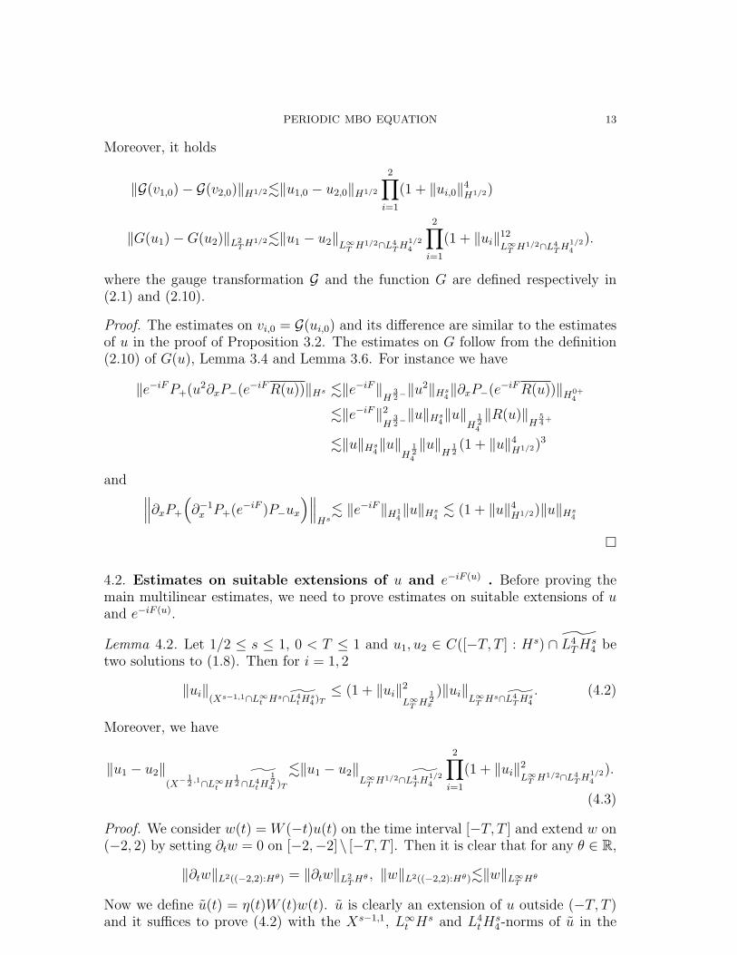
Moreover, it holds
‖G(v1,0)− G(v2,0)‖H1/2.‖u1,0 − u2,0‖H1/2
2∏i=1
(1 + ‖ui,0‖4H1/2)
‖G(u1)−G(u2)‖L2TH
1/2.‖u1 − u2‖L∞T H1/2∩L4TH
1/24
2∏i=1
(1 + ‖ui‖12
L∞T H1/2∩L4
TH1/24
).
where the gauge transformation G and the function G are defined respectively in(2.1) and (2.10).
Proof. The estimates on vi,0 = G(ui,0) and its difference are similar to the estimatesof u in the proof of Proposition 3.2. The estimates on G follow from the definition(2.10) of G(u), Lemma 3.4 and Lemma 3.6. For instance we have
‖e−iFP+(u2∂xP−(e−iFR(u))‖Hs .‖e−iF‖H
32−‖u2‖Hs
4‖∂xP−(e−iFR(u))‖H0+
4
.‖e−iF‖2
H32−‖u‖Hs
4‖u‖
H124
‖R(u)‖H
54+
.‖u‖Hs4‖u‖
H124
‖u‖H
12(1 + ‖u‖4
H1/2)3
and ∥∥∥∂xP+
(∂−1x P+(e−iF )P−ux
)∥∥∥Hs. ‖e−iF‖H1
4‖u‖Hs
4. (1 + ‖u‖4
H1/2)‖u‖Hs4
�
4.2. Estimates on suitable extensions of u and e−iF (u) . Before proving themain multilinear estimates, we need to prove estimates on suitable extensions of uand e−iF (u).
Lemma 4.2. Let 1/2 ≤ s ≤ 1, 0 < T ≤ 1 and u1, u2 ∈ C([−T, T ] : Hs) ∩ L4TH
s4 be
two solutions to (1.8). Then for i = 1, 2
‖ui‖(Xs−1,1∩L∞t Hs∩L4
tHs4)T≤ (1 + ‖ui‖2
L∞T H12x
)‖ui‖L∞T H
s∩L4TH
s4
. (4.2)
Moreover, we have
‖u1 − u2‖(X−
12 ,1∩L∞t H
12∩
˜L4tH
124 )T
.‖u1 − u2‖L∞T H
1/2∩ ˜L4TH
1/24
2∏i=1
(1 + ‖ui‖2
L∞T H1/2∩L4
TH1/24
).
(4.3)
Proof. We consider w(t) = W (−t)u(t) on the time interval [−T, T ] and extend w on(−2, 2) by setting ∂tw = 0 on [−2,−2]\ [−T, T ]. Then it is clear that for any θ ∈ R,
‖∂tw‖L2((−2,2):Hθ) = ‖∂tw‖L2TH
θ , ‖w‖L2((−2,2):Hθ).‖w‖L∞T Hθ
Now we define u(t) = η(t)W (t)w(t). u is clearly an extension of u outside (−T, T )and it suffices to prove (4.2) with the Xs−1,1, L∞t H
s and L4tH
s4-norms of u in the

14 Z. GUO, Y. LIN, L. MOLINET
left-hand side. First, using that ∂tw = 2W (−t)(P 6=c(u2)ux), we get
‖u‖Xs−1,1 .‖w‖L2((−2,2):Hs−1) + ‖∂tw‖L2((−2,2):Hs−1)
.‖u‖L2((−2,2):Hs−1) + ‖Dsx(u
3)‖L2Tx
+ ‖u‖2L∞T L
2x‖Ds
xu‖L2Tx
.‖u‖L2((−2,2):Hs−1) + ‖Dsxu‖L4
Tx∩L∞T L
2x‖u‖2
L∞T H12x
where in the last step we used Lemma 3.5 together with L∞t H1/2x ↪→ L8
tx. Second,
‖u‖L∞t Hs . ‖η(t)W (t)w(t)‖L∞t Hs? . ‖w‖L∞T Hs . ‖u‖L∞T Hs .
Third, we notice that
‖u‖L4tH
s4
. ‖u‖ ˜L4(]−T,T [;Hs4)
+ ‖W (t)w(t)‖ ˜L4(]−2,2[/]−T,T [;Hs4)
with w(t) = w(T ) for all t ∈]T, 2[ and w(t) = W (−T ) for all t ∈]−2,−T [. Therefore,in view of (3.4),
‖W (t)w(t)‖ ˜L4(]T,2[;Hs4)
= ‖W (t)w(T )‖ ˜L4(]T,2[;Hs4). ‖w(T )‖Hs = ‖u(T )‖Hs . ‖u‖L∞T Hs .
This completes the proof of (4.2). Finally the estimates for the difference is similarand thus will be omitted. �
Next, we prove the properties of the factor eikF .
Lemma 4.3. Let 1/2 ≤ s ≤ 1, 0 < T ≤ 1 and u1, u2 ∈ C([−T, T ] : Hs) ∩ L4TH
s4 be
two solutions to (1.8). Then for i = 1, 2
‖e−iF (ui)‖(L∞t H
s+1−∩X−12−,1)T
.1 + (1 + ‖ui‖6
L∞T H12∩L4
TH124
)‖ui‖L∞T Hs∩L4TH
s4. (4.4)
Moreover,
‖e−iF (u1) − e−iF (u2)‖(L∞t H
32−∩L4
tH32 ∩X−
12−,1)T
.‖u1 − u2‖L∞T H
12∩L4
TH124
2∏i=1
(1 + ‖u‖6
L∞T H12∩L4
TH124
) . (4.5)
Proof. We set z(t) = W (−t)e−iF on ]−T, T [ and than extend z on ]−2, 2[ by setting∂tz = 0 on [−2,−2]\ [−T, T ]. Then w = η(t)W (t)z(t) is an extension of e−iF outside(−T, T ). As in the previous lemma, for any θ ∈ R, it holds
‖w‖L∞t Hθ . ‖e−iF‖L∞T Hθ?
which together with (3.17)-(3.18) gives the estimate for the first term on the left-hand side of (4.4). Moreover,
‖w‖X−
12−,1. ‖e−iF‖
L2TH− 1
2−+ ‖(∂t +H∂2
x)e−iF‖
L2TH− 1
2−
.with
(∂t +H∂2x)e−iF = −ie−iFFt − iH
(e−iF
(2uux − i(P 6=c(u2))2
))

PERIODIC MBO EQUATION 15
According to the expression (2.2) of Ft, Lemma 3.4 and Lemma 3.8 , it holds
‖Ft‖L2TH− 1
2−+∥∥∥2uux + ik(P 6=c(u
2))2∥∥∥L2TH− 1
2−. ‖u‖4
L∞T H1/2 + ‖u‖2
L4TH
1/24
which yields the desired result by using (3.17) and again Lemma 3.4.For the difference estimate (4.5), the proof is similar by using (3.21)-(3.22). Thedetails are omitted. �
4.3. Multilinear estimates. With Lemmas 4.2-4.3 in hand, the following propo-sition enables us to treat the worst term of (4.1), that is N ν(u, v) with ν ∈ {0, 1}.
Proposition 4.4. Let 1/2 ≤ s ≤ 1, w1, w4 ∈ X−1/2−,1 ∩ L∞t Hs+1−x , u2, u3 ∈ Xs−1,1 ∩
L∞t Hsx ∩ L4
tHs4 and v5 ∈ X1/2,1/2 with compact support in time. Then it holds
∥∥∥∂νxP+
(∂−νx P+
(w1u2u3
)∂xP−(w4v5)
)∥∥∥Xs,− 1
2+
. ‖w1‖L∞t Hs+1−‖w4‖L∞T H1/2x‖v5‖X1/2,1/2
3∏i=2
‖ui‖L∞t H1/2x
+ ‖v5‖X1/2,1/2
∏i=1,4
(‖wi‖X−1/2−,1∩L∞t H
3/2−x
)×
∑2≤i 6=j≤3
(‖ui‖
X−1/2,1∩L∞t H1/2x ∩L4
tH1/2x
)(‖uj‖
Xs−1,1∩L∞t Hsx∩L4
tHs4
). (4.6)
Proof. We want to prove that
I :=∥∥∥∂νxP+
(∂−νx P+
(w1u2u3
)∂xP−(w4v5)
)∥∥∥Xs,− 1
2+
=∥∥∥ ∑N≥2,N123≥N,N45≤N123
∑Ni, 1≤i≤5
∂νxPNP+
(∂−νx PN123
(PN1w1PN2u2PN3u3
)∂xPN45P−(PN4w4PN5v5)
)∥∥∥Xs,−1/2+
.
By the triangle inequality we can separate this sum in different sums on disjointsubset of (2N)8. By symmetry we can assume that N2 ≤ N3.
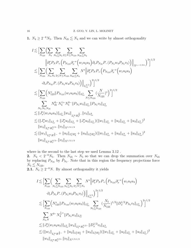
16 Z. GUO, Y. LIN, L. MOLINET
1. N4 ≥ 2−8N5. Then N45 . N4 and we can write by almost orthogonality
I .[∑N123
(∑N4
∑N5.N4
∑2≤N≤N123
∑N45.N4∥∥∥∂νxPNP+
(PN123∂
−νx
(w1u2u3
)∂xPN45P−(PN4w4PN5v5)
)∥∥∥Xs,−1/2+
)2]1/2
.[∑N123
(∑N4,N5
∑2≤N≤N123
∑N45.N4
N s∥∥∥∂νxPNP+
(PN123∂
−νx
(w1u2u3
)·∂xPN45P−(PN4w4PN5v5)
)∥∥∥L
4/3tx
)2]1/2
.[∑N123
(N s
123‖PN123(w1u2u3)‖L2tx
∑N≤N123
(N
N123
)s)2]1/2
∑N4,N5,N45
N0−45 N
1+4 N0−
5 ‖PN4w4‖L8tx‖PN5v5‖L8
tx
. ‖Jsx(w1u2u3)‖L2tx‖w4‖
L∞t H32−x
‖v5‖L8tx
. (‖Jsxw1‖L4tx
+ ‖Jsxu2‖L4tx
+ ‖Jsxu3‖L4tx
)(‖w1‖L8tx
+ ‖u2‖L8tx
+ ‖u3‖L8tx
)2
‖w4‖L∞t H3/2−x‖v5‖X1/2,1/2
. (‖w1‖L∞t H32−
+ ‖u2‖L4tH
s4
+ ‖u3‖L4tH
s4)(‖w1‖L8
tx+ ‖u2‖L8
tx+ ‖u3‖L8
tx)2
‖w4‖L∞t H3/2−x‖v5‖X1/2,1/2
where in the second to the last step we used Lemma 3.12 .2. N4 < 2−8N5. Then N45 ∼ N5 so that we can drop the summation over N45
by replacing PN45 by PN5 . Note that in this region the frequency projections forceN5 . N123.2.1. N4 ≥ 2−8N . By almost orthogonality it yields
I .[∑N123
( ∑N5.N123
∑N4.N5
∑2≤N≤N4
N s∥∥∥∂νxPNP+
(PN123∂
−νx
(w1u2u3
)·∂xPN5P−(PN4w4PN5v5)
)∥∥∥L
4/3tx
)2]1/2
.[∑N123
(N s
123‖PN123(w1u2u3)‖L2tx
∑N5.N123
(N5
N123
)1/2‖D1/2x PN5v5‖L4
tx
)2]1/2
∑N4,N
N0−N12
+
4 ‖PN4w4‖L∞tx
. ‖Jsx(w1u2u3)‖L2tx‖w4‖L∞t H3/2−
x‖D1/2
x v5‖L4tx
. (‖w1‖L∞t H32−
+ ‖u2‖L4tH
s4
+ ‖u3‖L4tH
s4)(‖w1‖L8
tx+ ‖u2‖L8
tx+ ‖u3‖L8
tx)2
‖w4‖L∞t H3/2−x‖v5‖X1/2,1/2
PERIODIC MBO EQUATION 17
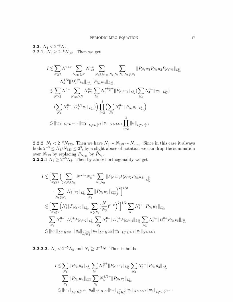
2.2. N4 < 2−8N .2.2.1. N1 ≥ 2−8N123. Then we get
I .∑N≥2
N s+ν∑
N123≥N
N−ν123
∑N1&N123
∑N2,N3,N4,N5.N1
‖PN1w1PN2u2PN3u3‖L2tx
·N1/25 ‖D1/2
x v5‖L4tx‖PN4w4‖L∞tx
.∑N≥2
N0−∑
N123≥N
N0−123
∑N1
Ns+ 1
2+
1 ‖PN1w1‖L4tx
(∑N4
N0−4 ‖w4‖L∞tx)
(∑N5
N0−5 ‖D1/2
x v5‖L4tx
)) 3∏i=2
(∑Ni
N0−i ‖PNiui‖L8
tx
). ‖w1‖L∞t Hs+1−‖w4‖L∞T H1/2
x‖v5‖X1/2,1/2
3∏i=2
‖u‖L∞t H
1/2x
2.2.2 N1 < 2−8N123. Then we have N3 ∼ N123 ∼ Nmax. Since in this case it alwayshods 2−3 ≤ N3/N123 ≤ 23, by a slight abuse of notation we can drop the summationover N123 by replacing PN123 by PN3 .2.2.2.1 N1 ≥ 2−5N5. Then by almost orthogonality we get
I .[∑N3≥2
( ∑2≤N.N3
N s+νN−ν3
∑N1,N2
‖PN1w1PN2u2PN3u3‖L
83tx
·∑N5.N1
N5‖v5‖L8tx
∑N4
‖PN4w4‖L∞tx)2]1/2
.[∑N3≥2
(N s
3‖PN3u3‖L4tx
∑N.N3
(N
N3
)s+ν)2]1/2∑
N1
N1+1 ‖PN1w1‖L4
tx∑N3
N0−2 ‖D0+
x PN2u2‖L8tx
∑N4
N0−4 ‖D0+
x PN4w4‖L∞tx∑N5
N0−5 ‖D0+
x PN5v5‖L8tx
. ‖w1‖L∞t H3/2−‖u3‖L4tH
s4
‖u2‖L∞t H1/2‖w4‖L∞t H1/2‖v5‖X1/2,1/2
2.2.2.2. N1 < 2−5N5 and N1 ≥ 2−5N . Then it holds
I .∑N2
‖PN2u2‖L4tx
∑N1
N12
+
1 ‖PN1w1‖L∞tx∑N3
N s−3 ‖PN3u3‖L4
tx∑N4
‖PN4w4‖L∞tx∑N5
N1/2−5 ‖PN5v5‖L4
tx
. ‖w1‖L∞t H3/2−x‖u2‖L∞t H1/2‖u3‖
L4tH
s4
‖v5‖X1/2,1/2‖w4‖L∞t H3/2−x
.

18 Z. GUO, Y. LIN, L. MOLINET
2..2.2.3 N1 < 2−5(N5 ∧N) and N2 ≥ 2−5(N5 ∧N).2.2.2.3.1 N2 ≥ 2−7N . Then either N3 ∼ N and then N3 ∼ N ∼ N2 which leads to
I .[∑N3≥2
( ∑N2∼N3
∑Ni.N2i∈{1,4,5}
∥∥∥∂νxPN3P+
(PN3∂
−νx
(PN1w1PN2u2PN3u3
)
· ∂xPN5P−(PN4w4PN5v5))∥∥∥
Xs,−1/2
)2]1/2
.[∑N3
( ∑N2∼N3
∑Ni.N2i∈{1,4,5}
N s3
∥∥∥PN1w1PN2u2PN3u3
∥∥∥L2tx
N5‖PN4w4PN5v5‖L4tx
)2]1/2
.[∑N3
N2s3 ‖PN3u3‖2
L4tx
(∑N1,N4
‖PN1w1‖L∞tx‖PN4w4‖L∞tx∑N2∼N3
∑N5.N3
(N3
N2
)1/2(N5
N3
)1/2
‖D1/2x PN2u2‖L4
tx‖PN5D
1/2x v5‖L4
)2]1/2
.‖u3‖L4tH
s4
‖D1/2x u2‖L4
tx‖D1/2
x v5‖L4tx‖w1‖L∞t H3/2−‖w4‖L∞t H3/2−
or N3 ∼ N5 and then we get
I .[∑N
( ∑N2&N
∑N3&N
∑Ni,i∈{1,4}
N s+νN1/2−ν3 ‖PN1w1‖L∞tx‖PN2u2‖L4
tx
‖PN3u3‖L4tx‖PN4w4‖L∞tx‖PN3D
1/2x v5‖L4
tx
)2]1/2
. ‖w1‖L∞t H1/2x‖w4‖L∞t H1/2
x
∑N3
N s3‖PN3u3‖L4
tx‖PN3D
1/2x v5‖L4
tx[∑N
( ∑N2&N
( NN2
)1/2
N1/22 ‖PN2u2‖L4
tx
)2]1/2
. ‖u3‖L4tH
s4
‖u2‖L4tH
1/24
‖D1/2x v5‖L4
tx‖w1‖L∞t H3/2−‖w4‖L∞t H3/2−
where, in the last step, we used Cauchy-Schwarz in N3 and that by discrete Younginequality
∥∥∥∑k∈Z
(2k−k2)1/2χ{k−k2≤5}‖J1/2x P2k2u2‖L4
∥∥∥l2(N). ‖J1/2
x u2‖L4tx.

PERIODIC MBO EQUATION 19
2.2.2.3.2. N2 < 2−7N . Then N2 ≥ 2−5N5 since we must have N5 ≤ 2−3N3. Thisforces N3 ∼ N so that we get
I .[∑N3
(∑N2
∑N5.N2
∑N1,N4
N s3
∥∥∥PN1w1PN2u2PN3u3
∥∥∥L2tx
N5‖PN4w4PN5v5‖L4tx
)2]1/2
. ‖w1‖L∞t H1/2x‖w4‖L∞t H1/2
x
[∑N3
N2s3 ‖PN3u3‖2
L4tx
]1/2
∑N2
∑N5.N2
(N5
N2
)1/2
‖J1/2x PN2u2‖L4
tx‖PN5D
1/2x v5‖L4
. ‖u3‖L4tH
s4
‖u2‖L4tH
1/24
‖D1/2x v5‖L4
tx‖w1‖L∞t H3/2−‖w4‖L∞t H3/2−
where in the last step we used the discrete Young inequality.2.2.2.4. (N1 ∨ N2) < 2−5(N ∧ N5). Here it is worth noticing that we can assumethat (N ∧ N5) ≥ 24 and the result follows directly from the lemma below and theproof of the proposition is completed. �
Lemma 4.5. Under the same hypotheses on ui as in Proposition, it holds
J :=[ ∑N≥24
( ∑(Ni)1≤i≤5∈ΛN
∥∥∥∂νxPNP+
(∂−νx PN3
(PN1w1PN2u2PN3u3
)
· ∂xPN5P−(PN4w4PN5v5))∥∥∥
Xs,−1/2+
)2]1/2
.3∏i=1
‖ui‖Z
where
ΛN :={
(N1, N2, N3, N4, N5) ∈ (2N ∪ {0})5, N3 ≥ 2−3N,
24 < N5 ≤ 4N3, (N1 ∨N2 ∨N4) < 2−5(N ∧N5)}.
Proof. It is worth noticing that, thanks to the frequency projections, N3 ∼ Nmax
and the resonance relation yields
|σmax| & |ξξ5| ≥ 2−2NN5 & (N ∧N5)N3 (4.7)
for all the contributions in J . First we can easily treat the contribution of the region{(τ, ξ), 〈τ − ξ|ξ|〉 ≥ 2−2NN5}. Indeed, we then get
J .∑N≥24
∑(N1,N2,N3,N4,N5)∈ΛN
(NN5)−12
+N1/25 N s+νN−s−ν3
‖PN3Dsxu3‖L4
tx‖D1/2
x PN5v5‖L4tx‖PN2u2‖L∞tx
∏i=1,4
‖PNiwi‖L∞tx
.∑N≥24
N−12
+‖u3‖L4tH
s4‖D1/2
x v5‖L4tx‖u2‖L∞t H1/2
x‖w1‖L∞t H1/2
x‖w4‖L∞t H1/2
x
which is acceptable. Therefore in the sequel we can assume that 〈τ − ξ|ξ|〉 <2−2NN5}. Now, for any fixed couple (N,N5) ∈ (2N)2, we split any function z ∈ L2
tx
into two parts related to the value of σ by setting
z = F−1(η2−4NN5
(τ − ξ|ξ|)z)
+ F−1(
(1− η2−4NN5(τ − ξ|ξ|))z
):= z + ˜z .
20 Z. GUO, Y. LIN, L. MOLINET
1. Contribution of ˜v5. We now control the contribution of ˜v5 to J in the followingway : either N ∼ N3 ∼ Nmax and we write
J .∑N≥24
∑N3∼N
∑Ni≤25N3i=1,3,4,5
N s(NN5)−1/2N1/25 N−s3
‖PN5˜v5‖X1/2,1/2‖PN3D
sxu3‖L4
tx‖PN2u2‖L∞tx
∏i=1,4
‖PNiwi‖L∞tx
.(∑N
N−12
+)‖˜v5‖X1/2,1/2‖u3‖L4tH
s4‖u2‖L∞t H1/2
x
∏i=1,4
‖wi‖L∞t H1/2x
or N5 ∼ N3 ∼ Nmax and we write
J .∑N≥24
∑N3
∑N5∼N3
∑Ni≤2−5Ni=1,2,4
N s(NN5)−1/2N1/25 N−s3
‖PN5˜v5‖X1/2,1/2‖PN3D
sxu3‖L4
tx‖PN2u2‖L∞tx
∏i=1,4
‖PNiwi‖L∞tx
.(∑N
N−12
+)‖v5‖X1/2,1/2‖u3‖L4tH
s4
‖u2‖L∞t H1/2x
∏i=1,4
‖wi‖L∞t H1/2x
where we apply Cauchy-Schwarz in N3 ∼ N5 in the last step.2. Contribution of v5.2.1 Contribution of ˜w1. We easily get
J .∑N
∑(N1,N2,N3,N4,N5)∈ΛN
((N ∧N5)N3)−1N12
+
1 N1−s5 N s
‖PN1˜w1‖X−1/2−,1‖PN3u3‖L∞tx‖PN5D
sxv5‖L4
tx‖PN2u2‖L∞tx‖PN4w4‖L∞tx
.∑N
N−12
+‖w1‖X−1/2−,1‖u3‖L∞t H
12x
‖v5‖Xs,1/2‖u2‖L∞t H1/2x‖w4‖L∞t H1/2
x
which is acceptable.2.2 Contribution of w1. To treat this contribution we will extensively use the fol-lowing lemma which is a direct application of the Marcinkiewicz multiplier theorem.
Lemma 4.6. For any p ∈]1,+∞[ there exists Cp > 0 such that for all N ≥ 1 and allL ≥ N2,∥∥∥F−1
tx
(φN(ξ)ηL(τ ∓ ξ2)f(τ, ξ)
)∥∥∥Lptx
≤ Cp ‖f‖Lptx , ∀f ∈ Lp(R2) . (4.8)
Proof. By Marcinkiewicz multiplier theorem (see for instance ([6],Corollary 5.2.5page 361)), it suffices to check that∣∣∣∂(α1,α2)
τ,ξ
(φN(ξ)ηL(τ ∓ ξ2)
)∣∣∣ . |ξ|α1|τ |α2 for |α| ≤ 2.
But this follows directly from the fact that for N2 ≤ L ,
d
dξ
(φN(ξ)ηL(τ ∓ ξ2)
)= O(N−1) and
d
dτ
(φN(ξ)ηL(τ ∓ ξ2)
)= O(L−1) .
�
PERIODIC MBO EQUATION 21
It is worth noticing that on ΛN , with N ≥ 24, it holds N2i ≤ 2−2NN5 for i ∈
{1, 2, 4}. Hence, in view of (4.8), for any 1 < p <∞, setting (z1, z2, z4) = (w1, u2, w4)it holds
‖PNiP∓z‖Lptx ≤ Cp ‖PNiP∓z‖Lptx .
and thus by the continuity of the Hilbert transform in Lp, 1 < p <∞,
‖PNi z‖Lptx ≤ Cp ‖PNiz‖Lptx . (4.9)
We separate the contribution of w1 in different sub-contributions.2.2.1 Contribution of ˜u2. Then we write
J .∑N
∑(N1,N2,N3,N4,N5)∈ΛN
((N ∧N5)N3)−1N12
+
2 N5NsN−s+1/63
‖PN2˜u2‖X−1/2−,1‖PN3D
s−1/6x u3‖L6
tx‖PN5 v5‖L24
tx‖PN1w1‖L24
tx‖PN2u2‖L∞tx‖PN4w4‖L∞tx
.∑N
N−16‖w1‖L24
tx‖Ds
xu3‖L6tL
3x‖v5‖X1/2,1/2‖u2‖X−1/2−,1‖w4‖L∞t H1/2
x
.‖w1‖L∞t H1/2x‖u3‖L∞t Hs∩L4
tHs4‖v5‖X1/2,1/2‖u2‖X−1/2−,1‖w4‖L∞t H1/2
x
where we used Sobolev inequalities and (4.9) in the last to the last step.2.2.2 Contribution of u2.2.2.2.1 Contribution of ˜w4. This subcontribution can be estimated in the same wayby
J .∑N
∑(N1,N2,N3,N4,N5)∈ΛN
((N ∧N5)N3)−1N12
+
4 N5NsN−s+1/63
‖PN2˜w4‖X−1/2−,1‖PN3D
s−1/6x u3‖L6
tx‖PN5 v5‖L36
tx‖PN1w1‖L36
tx‖PN2u2‖L36
tx
.‖w1‖L∞t H1/2x‖u3‖L∞t Hs∩L4
tHs4‖v5‖X1/2,1/2‖u2‖L∞t H1/2
x‖w4‖X−1/2−,1
2.2.2.2 Contribution of w4. Since max(|σi|) < 2−2NN5, we only have to consider˜u3 in this contribution. Either N ∼ N3 and then
J2 .∑N3
( ∑(N1,N2,N3,N4,N5)∈ΛN3
N s3 (N3N5)−1N
2/35 N1−s
3
‖PN3˜u3‖Xs−1,1‖PN5D
1/3x v5‖L6
tx‖PN2u2‖L36
tx
∏i=1,4
‖PNiwi‖L36tx
)2
.(∑N3
‖PN3u3‖Xs−1,1
)2
‖v5‖2X1/2,1/2‖u2‖2
L∞t H1/2x
∏i=1,4
‖wi‖2
L∞t H1/2x
or N5 ∼ N3. In this last case we first notice that X0,3/8 ↪→ L4tx and that for any
fixed 2 < p <∞, X0,1/2−T ↪→ LpTL
2x. Therefore by interpolation, Sobolev inequalities

22 Z. GUO, Y. LIN, L. MOLINET
and duality we infer that L65Tx ↪→ X
− 16−,−1/2+
T . We thus get
J2 .∑N
(∑N3
∑(N∨N1∨N2∨N4).N3
N sN16
+(NN3)−1N1/23 N1−s
3
‖PN3˜u3‖Xs−1,1‖PN3D
1/2x v5‖L4
tx‖PN2u2‖L36
tx
∏i=1,4
‖PNiwi‖L36tx
)2
.∑N
N−16
+(∑N3
‖PN3u3‖Xs−1,1‖PN3D1/2x v5‖L4
tx
)2
‖u2‖2
L∞t H1/2x
∏i=1,4
‖wi‖2
L∞t H1/2x
.‖u3‖2Xs−1,1‖v5‖2
X1/2,1/2‖u2‖2
L∞t H1/2x
∏i=1,4
‖wi‖2
L∞t H1/2x
where we apply Cauchy-Scwharz in N3 in the last step. �
Finally, this last proposition together with Lemmas 4.3 enables to treat the termcontaining B(u, u) in (4.1).
Proposition 4.7. Let 1/2 ≤ s ≤ 1, w1 ∈ X−1/2−,1 ∩ L∞t Hs+1−x , and ui ∈ Xs−1,1 ∩
L4tH
s4 ∩ L∞t Hs, i = 2, 3, 4. with compact support in time such that u2 and u3 are
real-valued. Then it holds∥∥∥w1u2B(u3, u4)∥∥∥Xs,− 1
2+.‖w1‖X−1/2−,1‖u2‖L∞t H
12‖u3‖L∞t H
12‖u4‖L4
tHs4
+ ‖w1‖L∞t H
32−x
∑(2≤i 6=j 6=q≤4)
‖ui‖X−
12−,1∩
˜L4tH
124 ∩L∞t H
12
· ‖uj‖X−
12 ,1∩
˜L4tH
124 ∩L∞t H
12
‖uq‖Xs−1,1∩L4
tHs4∩L∞t Hs
. (4.10)
Proof. Recall that B(u, v) = −i∂−1x (P+uxP+vx) + i∂−1
x (P−uxP−vx). By symmetry itthus suffices to estimate
I :=∥∥∥w1u2∂
−1x (P+∂xu3P+∂xu4)
∥∥∥Xs,− 1
2+
=∥∥∥ ∑N≥1,N1,N2,N3,N4,N34≥(N3∨N4)/2
PN
(PN1w1PN2u2
· PN34∂−1x (P+∂xPN3u3P+∂xPN4u4)
)∥∥∥Xs,− 1
2+.
By symmetry we can assume that N3 ≤ N4 and thus we must have N34 ∼ N4. Wecan thus drop the summation over N34 and replace PN34 by PN4 .
By the triangle inequality we can separate this sum in different sums on disjointsubset of (2N)5.

PERIODIC MBO EQUATION 23
1. N1 ≥ 2−8N . Then we have
I .∑N
∑N1≥2−8N
∑N2,N3,N4
N s∥∥∥PN(PN1w1PN2u2PN4∂
−1x (P+∂xPN3u3P+∂xPN4u4)
)∥∥∥L
4/3tx
.∑
N≤28N1
∑N2,N3,N4
‖PN1w1‖L∞t Hs+8‖PN2u2‖L∞t L8
x?
4∏i=3
‖PNiui‖L4tH
12−4
?
.‖w1‖L∞t H
32−x
‖u2‖L∞t H
12x
4∏i=3
‖PNiui‖L4tH
124
? .
2. N1 < 2−8N and N1 ≥ 2−5N3. Then either N4 & N ∨N2 and it holds
I .[∑N
( ∑N4&N
∑N1<2−8N
∑N3≤25N1
∑N2
N s∥∥∥PN(PN1w1PN2u2
· PN4∂−1x (P+∂xPN3u3P+∂xPN4u4)
)∥∥∥L
4/3tx
)2] 12
.(∑
N
( ∑N4&N
(N
N4
)2s‖Jsxu4‖2L4tx
) 12∑
N1,N2,N3
‖PN1w1‖L∞t H14‖PN2u2‖L∞t L8
x‖PN2u3‖L∞t L8
x?
.‖w1‖L∞t H
32−x
‖u2‖L∞t H
12x
‖u3‖L∞t H
12x
‖u4‖L4tH
s4
.
or N2 & N ∨N4 and it holds
I .[∑N
( ∑N2&N
∑N1<2−8N
∑N3≤25N1
∑N4
N s∥∥∥PN(PN1w1PN2u2
· PN4∂−1x (P+∂xPN3u3P+∂xPN4u4)
)∥∥∥L
4/3tx
)2] 12
.(∑
N
( ∑N2&N
(N
N2
)2s‖Jsxu2‖2L4tx
) 12∑
N,N3,N4
‖PN1w1‖L∞t H14?
4∏i=3
‖PNivi‖L∞t L8x?
.‖w1‖L∞t H
32−x
‖u2‖L4tH
s4
4∏i=3
‖ui‖L∞t H
12x
.
24 Z. GUO, Y. LIN, L. MOLINET
3. N1 < (2−8N ∧ 2−5N3).3.1 N2 ≥ 2−8N . Then we have
I .(∑
N
[ ∑N2≥2−8N
∑N3,N4
∑N1
N s∥∥∥PN(PN1w1PN2u2
· PN3∂−1x (P+∂xPN3u3P+∂xPN4u4)
)∥∥∥L
4/3tx
]2)1/2
.‖w1‖L∞t H1x
(∑N
[ ∑N2≥2−8N
(N
N2
)sN s2‖PN2u2‖L4
tx
]2)1/2
·∑N4
N−14 ‖PN4(P+∂xPN3u3P+∂xPN4u4)‖L2
tx
.‖w1‖L∞t H1x‖u2‖
L4tH
s4
∑N4
‖PN4D1/2x u4‖L4
tx
∑N3≤N4
(N3
N4
)1/2‖PN3D1/2x u3‖L4
tx
.‖w1‖L∞t H1x‖u2‖
L4tH
s4
‖D1/2x u3‖L4
tx‖D1/2
x u4‖L4tx.
where we use two times the discret Young inequality.3.2 N2 < 2−8N and N2 ≥ 2−5N3. Then we must have N ∼ N4 and thus
I .(∑N4
[∑N1,N3
∑N2≥2−5N3
N−1/22 N
1/23 ‖PN1w1‖L∞tx‖PN2J
1/2x u2‖L4
tx
· ‖PN3D1/2x u3‖L4
tx‖PN4D
sxu4‖L4
tx
]2)1/2
.‖w1‖L∞t H1x
(∑N4
‖DsxPN4u4‖2
L4tx
)1/2
·∑N2
‖PN2J1/2x u2‖L4
tx
∑N3≤25N2
(N3
N2
)1/2‖PN3D1/2x u3‖L4
tx
.‖w1‖L∞t H1x‖u2‖
L4tH
1/24
‖u3‖L4tH
1/24
‖u4‖L4tH
s4
.
3.3 N2 < (2−8N ∧ 2−5N3). Then N ∼ N4 and the resonance relation yields
|σmax| & |ξ3ξ4| ≥ 2−2N3N4 . (4.11)
First we can easily treat the contribution of the region {(τ, ξ), 〈τ−ξ|ξ|〉 ≥ 2−2N3N4}.Indeed, we then get
I .∑N4
∑N3.N4
∑N1∨N2.N3
N1/23 (N3N4)−1/2+‖w1‖L∞t H1
x‖PN2u2‖L∞tx
· ‖PN3D1/2x u3‖L4
tx‖PN4J
sxu4‖L4
tx
.‖w1‖L∞t H1x‖D1/2
x u3‖L4tx‖u4‖L4
tHs4
∑N2
N−1/2+2 ‖PN2u2‖L∞tx
.‖w1‖L∞t H1x‖u2‖L∞t H1/2
x‖u3‖
L4tH
124
‖u4‖L4tH
s4.
which is acceptable. Therefore in the sequel we can assume that 〈τ − ξ|ξ|〉 <2−2N3N4}. We now split v1, u2 and u3 into two parts related to the value of σi by

PERIODIC MBO EQUATION 25
setting
z = F−1(η2−4N3N4
(τ − ξ|ξ|)z)
+ F−1(
(1− η2−4N3N4(τ − ξ|ξ|))z
):= z + ˜z .
It is worth noticing that in this region N2i << N3N4 for i = 1, 2, 3. Therefore
Lemma 4.8 holds for w1, u2 and u3.3.3.1. Contribution of ˜w1. We first control the contribution of ˜w1 to I in thefollowing way :
I .∑N4
∑N3.N4
∑N1∨N2.N3
N1/2+1 N3(N3N4)−1‖PN1
˜w1‖X−1/2−,1
· ‖PN2u2‖L∞tx‖PN3u3‖L∞tx‖PN4Jsxu4‖L4
tx
.‖w1‖X−1/2−,1‖u2‖L∞t H12‖u3‖L∞t H
12‖u4‖L4
tHs4.
3.3.2. Contribution of w1.3.3.2.1 Contribution of ˜u2. In the same way, using Sobolev inequality, we have
I .∑N4
∑N3.N4
∑N1∨N2.N3
N1/2+1 N3(N3N4)−1N
1/64 ‖PN1w1‖L12
tx‖PN2
˜u2‖X−1/2−,1
‖PN3u3‖L∞tx‖PN4Js−1/6x u4‖L6
tx
.‖w1‖L∞t H12‖u2‖X−1/2−,1‖u3‖L∞t H
12‖u4‖L∞t Hs∩L4
tHs4.
3.3.2.2 Contribution of u2.3.2.2.2.1 Contribution of ˜u3.
I .∑N4
∑N3.N4
∑N1∨N2.N3
N3/23 (N3N4)−1N
1/64 ‖PN1w1‖L24
tx
· ‖PN1u2‖L24tx‖PN3u3‖X−1/2,1‖PN4J
s−1/6x u4‖L6
tx
.‖w1‖L∞t H12‖u2‖L∞t H
12‖u3‖X−1/2,1‖u4‖L∞t Hs∩L4
tHs4.
3.2.2.2.2 Contribution of u3. Since max(|σi|) ≥ 2−2N3N4, it remains to treat thesubcontribution of ˜u4. We easily obtain
I2 .∑N4
( ∑N3.N4
∑N1∨N2.N3
N2/33 N4(N3N4)−1‖PN1w1‖L24
tx
· ‖PN1u2‖L24tx‖PN3D
1/3x P+u3‖L6
tx‖PN4
˜u4‖Xs−1,1
)2
.(‖w1‖L∞t H
12‖u2‖L∞t H
12‖u3‖
L∞t H12∩L4
tH124
‖u4‖Xs−1,1
)2
.
Therefore, we complete the proof. �
Acknowledgment. Z. Guo is supported in part by NNSF of China (No. 11001003,No. 11271023).
References
[1] L. Abdelouhab, J. Bona, M. Felland, and J.-C. Saut, Nonlocal models for nonlinear dispersivewaves, Physica D. Nonlinear Phenomena 40 (1989), 360–392.
[2] T. B. Benjamin, Internal waves of permanent form in fluids of great depth, J. Fluid Mech. 29(1967), 559–592.

26 Z. GUO, Y. LIN, L. MOLINET
[3] J. Bourgain, Fourier transform restriction phenomena for certain lattice subsets and applica-tions to nonlinear evolution equations I, II. Geom. Funct. Anal., 3 (1993), 107-156, 209-262.
[4] N. Burq, and F. Planchon, On well-posedness for the Benjamin-Ono equation, Math. Annal.440 (2008), 497–542.
[5] J. Ginibre, Le probleme de Cauchy pour des EDP semi-lineaires periodiques en variablesd’espace (d’apres Bourgain), in Seminaire Bourbaki 796, Asterique 237, 1995, 163–187.
[6] L. Grafacos, Classical and Modern Fourier Analysis, Pearson/Prentice Hall, 2004.[7] Z. Guo, Local wellposedness and a priori bounds for the modified Benjamin-Ono equation,
Advances in Differential Equations, 16/11-12 (2011), 1087–1137.[8] S. Herr, On the Cauchy problem for the derivative nonlinear Schrodinger equation with periodic
boundary condition, Int. Math. Res. Not., 2006:Article ID 96763, 33 pages, 2006.[9] A. Ionescu and C. Kenig, Global well-posedness of the Benjamin-Ono equation in low-regularity
spaces, J. Amer. Math. Soc. 20 (2007), 753–798.[10] R. Iorio Jr., On the Cauchy problem for the Benjamin-Ono equation, Comm. Part. Diff. Eqs.
11 (1986), 1031-1081.[11] T. Kato and G. Ponce, Commutator estimates and the Euler and Navier-Stokes equations,
Comm. Pure Appl. Math. 41 (1988), 891–907.[12] C. Kenig and K. Koenig, On the local well-posedness of the Benjamin-Ono and modified
Benjamin-Ono equations, Math. Res. Let. 10 (2003), 879-895.[13] C. Kenig, G. Ponce, and L. Vega, Well-posedness and scattering results for the generalized
Korteweg-de Vries equation via the contraction principle, Comm. Pure Appl. Math. 46 (1993),527–620.
[14] C. Kenig, G. Ponce, and L. Vega, On the generalized Benjamin-Ono equation, Tran. Amer.Math. Soc. 342 (1994), 155–172.
[15] C. Kenig and H. Takaoka, Global wellposedness of the Modified Benjamin-Ono equation withinitial data in H1/2, Int. Math. Res. Not. 2006 (2006), 1–44.
[16] C. Kenig, Y. Martel and L. Robbiano, Local well-posedness and blow up in the energy spacefor a class of L2 critical dispersion generalized Benjamin-Ono equations, Ann. Inst. HenriPoincare, Anal. Non Linaire 28 (2011), 853-887 .
[17] H. Koch, and N. Tzvetkov, On the local well-posedness of the Benjamin-Ono equation inHs(R), Int. Math. Res. Not. 2003 (2003), 1449–1464.
[18] L. Molinet and D. Pilod, The Cauchy problem for the Benjamin-Ono equation in L2 revisited,Analysis & PDE 5 (2012), 365–395.
[19] L. Molinet and F. Ribaud, Well-posedness results for the generalized Benjamin-Ono equationwith arbitary large initial data, Int. Math. Res. Not. 2004 (2004), 3757–3795.
[20] L. Molinet and F. Ribaud, Well-posedness results for the generalized Benjamin-Ono equationwith small initial data, J. Math. Pures Appl. 83 (2004), 277–311.
[21] L. Molinet, Global well-posedness in the energy space for the Benjamin- Ono equation on thecircle, Math. Ann. 337 (2007), 353C383.
[22] L. Molinet, Global well-posedness in L2 for the periodic Benjamin-Ono equation, Amer. J.Math. 130 (2008), 635–683.
[23] L. Molinet and F. Ribaud, Well-posedness in H1 for the (generalized) Benjamin-Ono equationon the circle, DCDS 23 (2009), 1295-1311.
[24] L. Molinet, Sharp ill-posedness result for the periodic Benjamin-Ono equation, Journal ofFunctional Analysis 257 (2009) 3488–3516.
[25] H. Ono, Algebraic solitary waves in stratified fluids, J. Phys. Soc. Japan 39 (1975), 1082–1091.[26] G. Ponce, On the global well-posedness of the Benjamin-Ono equation, Diff. Int. Eqs 4 (1991),
527–542.[27] T. Tao, Global well-posedness of the Benjamin-Ono equation in H1(R), J. Hyper. Diff. Eqs 1
(2004), 27–49.
1LMAM, School of Mathematical Sciences, Peking University, Beijing 100871,China
PERIODIC MBO EQUATION 27
2Beijing International Center for Mathematical Research, Beijing 100871, ChinaE-mail address: [email protected], [email protected]
3Universite Francois Rabelais Tours, Federation Denis Poisson-CNRS, Parc Grand-mont, 37200 Tours, France
E-mail address: [email protected]
Copyright © 2022 FDOKUMEN