WELL POSEDNESS AND THE GLOBAL ATTRACTOR OF SOME QUASI-LINEAR PARABOLIC EQUATIONS WITH NONLINEAR...
35
Differential and Integral Equations Volume xx, Number xxx, , Pages xx–xx WELL-POSEDNESS AND THE GLOBAL ATTRACTOR OF SOME QUASI-LINEAR PARABOLIC EQUATIONS WITH NONLINEAR DYNAMIC BOUNDARY CONDITIONS Ciprian G. Gal Department of Mathematics, University of Missouri Columbia, MO, 65211 Mahamadi Warma Department of Mathematics, University of Puerto Rico Rio Piedras Campus, San Juan, PR, 00931 (Submitted by: Jerome A Goldstein) Abstract. We consider a quasi-linear parabolic equation with nonlinear dynamic boundary conditions occurring as generalizations of semilinear reaction-diffusion equations with dynamic boundary conditions and var- ious other phase-field models, such as the isothermal Allen-Cahn equa- tion with dynamic boundary conditions. We thus formulate a class of initial and boundary value problems whose global existence and unique- ness is proven by means of an appropriate Faedo-Galerkin approximation scheme developed for problems with dynamic boundary conditions. We analyze the asymptotic behavior of the solutions within the theory of infinite-dimensional dynamical systems. In particular, we demonstrate the existence of the global attractor. 1. Introduction A well-known mathematical model which describes the behavior of the phases in the absence of temperature variations and mechanical stresses, is given by the Allen-Cahn equation (see, e.g., [1]), which is given by ∂ t φ − ∆φ + f 1 (φ)= g 1 (x) , in Ω × (0, +∞), (1.1) where Ω is a bounded domain in R 3 . Here, φ is the order parameter, g 1 is an external force and f 1 is the derivative of a potential function F 1 , which accounts for the presence of different phases. For instance, F 1 can be a loga- rithmic potential which is usually approximated by a double well potential, i.e., F 1 (s)= s 2 − 1 2 . Accepted for publication: July 2009. AMS Subject Classifications: 35B41, 35K55, 37L30, 80A22. 1
Transcript of WELL POSEDNESS AND THE GLOBAL ATTRACTOR OF SOME QUASI-LINEAR PARABOLIC EQUATIONS WITH NONLINEAR...

Differential and Integral Equations Volume xx, Number xxx, , Pages xx–xx
WELL-POSEDNESS AND THE GLOBAL ATTRACTOR OFSOME QUASI-LINEAR PARABOLIC EQUATIONS WITH
NONLINEAR DYNAMIC BOUNDARY CONDITIONS
Ciprian G. GalDepartment of Mathematics, University of Missouri
Columbia, MO, 65211
Mahamadi WarmaDepartment of Mathematics, University of Puerto Rico
Rio Piedras Campus, San Juan, PR, 00931
(Submitted by: Jerome A Goldstein)
Abstract. We consider a quasi-linear parabolic equation with nonlineardynamic boundary conditions occurring as generalizations of semilinearreaction-diffusion equations with dynamic boundary conditions and var-ious other phase-field models, such as the isothermal Allen-Cahn equa-tion with dynamic boundary conditions. We thus formulate a class ofinitial and boundary value problems whose global existence and unique-ness is proven by means of an appropriate Faedo-Galerkin approximationscheme developed for problems with dynamic boundary conditions. Weanalyze the asymptotic behavior of the solutions within the theory ofinfinite-dimensional dynamical systems. In particular, we demonstratethe existence of the global attractor.
1. Introduction
A well-known mathematical model which describes the behavior of thephases in the absence of temperature variations and mechanical stresses, isgiven by the Allen-Cahn equation (see, e.g., [1]), which is given by
∂tφ−∆φ + f1 (φ) = g1 (x) , in Ω× (0, +∞), (1.1)
where Ω is a bounded domain in R3. Here, φ is the order parameter, g1 is
an external force and f1 is the derivative of a potential function F1, whichaccounts for the presence of different phases. For instance, F1 can be a loga-rithmic potential which is usually approximated by a double well potential,i.e., F1 (s) =
s2 − 1
2.
Accepted for publication: July 2009.AMS Subject Classifications: 35B41, 35K55, 37L30, 80A22.
1

2 Ciprian G. Gal and Mahamadi Warma,
While equation (1.1) has been extensively studied in the literature, thefollowing quasi-linear reaction-diffusion equation
∂tφ−∆pφ + f1 (φ) = g1 (x) , in Ω× (0, +∞), (1.2)
has received less attention and it has only recently captured the attentionof mathematicians (see, e.g., [2, 7, 8, 9, 11, 37, 45, 50] and the referencestherein). Above, in (1.2), the operator ∆p denotes the p-Laplace opera-tor, which is defined as ∆pu = div(|∇u|p−2∇u), p > 1. It is obvious that(1.2) reduces to (1.1) when p = 2. Regarding suitable boundary conditionsfor equations (1.1) or (1.2), the usual ones considered in the literature areDirichlet or Neumann. These standard boundary conditions together with(1.2) result in the fact that the following energy functional is decreasing:
EΩ (φ) :=
Ω
1p|∇φ|p + F1 (φ)− g1 (x)φ
dx, (1.3)
where, for simplicity, we take F1(r) = r0 f1(ζ)dζ. This can be easily checked
by differentiating the expression in (1.3) with respect to t, then using (1.2)and the boundary conditions (as long as a smooth solution exists). The ex-istence and the asymptotic behavior of strong solutions for (1.2), subject toDirichlet or Neumann boundary conditions were already studied by [4], [9],[34], [40] (and the references therein) in the reflexive Banach space frame-work. However, not much seems to be known about the existence, regularityand long term dynamics of (1.2), despite some classical results and recentresults from [5, 6, 7, 14, 36] (and their references).
In this article, motivated by many applications in the theory of phasetransitions phenomena, we plan to investigate (1.2), subject to dynamicboundary conditions. It has been recently discovered by physicists that, asfar as the Allen-Cahn equation (and some Cahn-Hilliard equations, cf. e.g.,[10, 24, 25, 27, 28, 29, 43] and their references) is concerned, for certainmaterials a dynamical interaction with the walls (i.e., with Γ := ∂Ω) mustbe taken into account (see, e.g., [20, 21, 22, 46] and their references). Inother words, the following energy functional should be added to (1.3):
EΓ (φ) :=
Γ[F2 (φ)− g2 (x)φ] dS, (1.4)
to form a total energy functional
E (φ) := EΩ (φ) + EΓ (φ) , (1.5)
where in (1.4) we neglect potential forces that account for surface diffusion;see however, Remark 3.13. Here, F2 is a nonlinear function such that F2(r) =
Nonlinear dynamic boundary conditions 3
r0 f2(ζ)dζ. We need to derive the physically correct boundary condition for
(1.2) such that the function E (φ) is decreasing for all time t ≥ 0. Usingintegration by parts, we proceed by formally calculating the time derivativeof E (φ) , for a smooth solution φ, as follows:d
dtE(φ(t)) =
Ω
|∇φ(t)|p−2∇φ(t) ·∇∂tφ(t) + f1 (φ(t)) ∂tφ(t)− g1∂tφ(t)
dx
+
Γ[f2 (φ(t)) ∂tφ(t)− g2∂tφ(t)] dS
=
Ω(−∆pφ(t) + f1 (φ(t))− g1) ∂tφ(t)dx
+
Γ
|∇φ(t)|p−2
∂nφ(t) + f2 (φ(t))− g2
∂tφ(t)dS
= −
Ω|∂tφ(t)|2 dx−
Γ|∂tφ(t)|2 dS ≤ 0, for all t ≥ 0. (1.6)
As a consequence, one deduces a dynamic boundary condition of the form
∂tφ + |∇φ|p−2∂nφ + f2 (φ) = g2 (x) , on Γ× (0, +∞). (1.7)
Phenomenologically speaking, the boundary condition (1.7) means that thedensity of the binary mixture at the surface relaxes towards equilibrium witha rate proportional to the driving force given by the Frechet derivative of thefree energy functional EΓ. The term |∇φ|p−2
∂nφ is due to the contributioncoming from the variation of the free energy functional EΩ. Here, ∂nφ denotesthe normal derivative of the function φ in direction of the outer normal vectorn. A physical interpretation of the dynamic boundary condition (1.7), in thecase p = 2, for linear heat equations was given in [32]. We point out thatthis type of boundary conditions are also used for modelling various physicalsituations including fluid diffusion within a (semi)permeable boundary (see,e.g., [12, 35, 38]) or several situations when the heat flow inside the domain Ωis subject to nonlinear heating or cooling at the boundary (see, e.g., [17, 18]).
This paper is concerned with the analysis of the system (1.2), (1.7), subjectto the initial condition
φ|t=0 = φ0. (1.8)Problems such as (1.2), (1.7)-(1.8) have already been partially examined in[10, 27, 28] within the theory of phase transitions, [13, 19, 23, 48, 49] andtheir references, always in the case p = 2, assuming that the nonlinearitiesf1 and f2 satisfy suitable assumptions. Such systems have also been inves-tigated for general p in a number of papers (see, for instance, [15, 16, 47]

4 Ciprian G. Gal and Mahamadi Warma,
and their references), where these contributions are mainly concerned withexistence and uniqueness issues. Let us point out some of the main difficul-ties in dealing with the boundary conditions (1.7). It is worth mentioningthat the issue of well-posedness for problem (1.2), (1.7)-(1.8), even in thecase p = 2, seems to be hard in general since standard techniques based onthe use of fractional powers operators or monotone operator theory cannotbe exploited. Indeed, our functions f1 and f2 are not monotone in general,even though the perturbation theory of maximal monotone operators can beemployed to deal with globally bounded perturbations of monotone opera-tors, but this always requires additional assumptions on the nonlinearities(see, e.g., [47]; cf. also [6] for standard boundary conditions). In particular,assuming f1 = g1 = g2 ≡ 0, f2 is a maximal monotone graph with f2 (0) = 0and by taking slightly regular initial data φ0, the author of [47] proves thatproblem (1.1), (1.7)-(1.8) possesses a unique (strong) solution in a suitablesense (cf. [47, Theorem 2.1 and Corollary 3.3]). However, in view of applica-tions to problems in phase separation and heat flow, it is desirable to workin less regular phase spaces (typically, in L
2(Ω)). This represents the maingoal of the paper. By showing that the principal part of equation (1.2) ismonotone in an appropriate Hilbert space setting and by making general hy-potheses on p, f1 and f2 (see Definition 2.1 below), so that the growth of thenonlinearities f1, f2 is dominated by a suitable version of the p-Laplacian,we first prove the well-posedness of the problem (see Theorem 2.6). Then wewant to establish the existence of the global attractor (see Corollary 3.11).The key step in the proofs is the construction of a new approximation schemethat can be employed when dealing with parabolic equations with dynamicboundary conditions. Such scheme was already successfully applied to a cou-pled system of parabolic equations involving a Cahn-Hilliard equation (see,e.g., [25]). However, with respect to the standard results, our problem (1.2),(1.7)- (1.8) has different features arising from the nature of the boundaryconditions which are now dynamic for φ. In particular, making use of theabove scheme, we can rigorously now prove for the first time the existenceof (unique) weak solutions to our system in a suitable Hilbert space, underminimal assumptions on the structural parameters of the problem (comparewith [47]).
We outline the plan of the paper, as follows. In Section 2, we intro-duce some notations and preliminary facts, then we show the existence anduniqueness of solutions to our system (1.2), (1.7)- (1.8), using a suitableFaedo-Galerkin approximation scheme. Section 3 is devoted to the existence

Nonlinear dynamic boundary conditions 5
of a bounded absorbing set and, then, of the global attractor. Some regu-larity properties of the weak solutions and hence of the global attractor willbe also derived.
2. Well-posedness
To establish the well-posedness of problem (1.2), (1.7)-(1.8) we need tointroduce some preliminary results. Using sufficiently strong global a prioriestimates, we will be able to prove well-posedness of our problem in a suit-able Sobolev space setup. Let Ω ⊂ RN be a bounded smooth domain withboundary Γ := ∂Ω. For k ∈ N0 := N∪ 0 and p ≥ 1, we define the Sobolevspaces W
k,p(Ω) and Wk,p(Γ) to be respectively the completion of C
k(Ω) andC
k(Γ), with respect to the norm
uW k,p(Ω) :=
0≤|α|≤k
Ω|∇α
u|p dx
1/p,
and
uW k,p(Γ) :=k
j=0
Γ|∇j
Γu|p dS
1/p.
Here, dx denotes the Lebesgue measure on Ω and dS denotes the naturalsurface measure on Γ. For p ∈ (1,∞) we define the fractional order Sobolevspace
W1− 1
p ,p(Γ) :=
u ∈ Lp(Γ) :
Γ
Γ
|u(x)− u(y)||x− y|1−
1p
p 1|x− y|N−1
dSx dSy < ∞
.
Since Ω has a smooth boundary, it is well-known that
W1,p(Ω) → L
ps(Ω), (2.1)
where ps := Np/(N − p) if p < N and 1 ≤ ps < ∞ if p = N . If p > N , onehas that W
1,p(Ω) is continuously embedded into C0,1−N
p (Ω). Moreover, onehas the following continuous embedding,
W1,p(Ω) → W
1− 1p ,p(Γ) → L
qs(Γ), (2.2)
where qs = (N − 1)p/(N − p) if p < N and 1 ≤ qs < ∞ if N = p. Fromnow on, we denote by ·W k,p(Ω) and ·W k,q(Γ) the norms on W
k,p (Ω) andW
k,q (Γ) , respectively. Also, ·, ·s and ·, ·s,Γ stand for the usual scalarproduct in L
s (Ω) and Ls (Γ), respectively.

6 Ciprian G. Gal and Mahamadi Warma,
The natural space for problem (1.2), (1.7)-(1.8) turns out to be
Xs := Ls(Ω)⊕ L
s(Γ) = F = (f, g) : f ∈ Ls(Ω), g ∈ L
s(Γ), s ∈ [1,+∞] ,
endowed with the norm defined through
FsXs =
Ω|f (x)|s dx +
Γ|g(x)|s dSx, (2.3)
if s ∈ [1,∞), and
FX∞ := maxfL∞(Ω), gL∞(Γ).
Identifying each function u ∈ W1,p(Ω) with the vector U := (u, u|Γ), it is
easy to see that W1,p(Ω) is a dense subspace of Xs for s ∈ [1,∞). Moreover,
one has thatXs = L
sΩ, dµ
, s ∈ [1, +∞] ,
where the measure dµ = dx|Ω ⊕ dS|Γ on Ω is defined for any measurable setA ⊂ Ω by µ(A) = |A ∩ Ω| + S(A ∩ Γ). Identifying each function θ ∈ C
Ω
with the vector Θ =θ|Ω, θ|Γ
∈ C
Ω
× C (Γ), one also has that C(Ω) is
a dense subspace of Xs for every s ∈ [1,∞) and a closed subspace of X∞.Next, for each p > 1, we let Vp = U := (u, u|Γ) : u ∈ W
1,p(Ω) and endowit with the norm ·Vp given by
u, u|Γ
Vp = uW 1,p(Ω) +
u|Γ
W 1−1/p,p(Γ).
It easy to see that we can identify Vp with W1,p (Ω)⊕W
1−1/p,p (Γ) under thisnorm. Moreover, since W
1,p(Ω) → W1−1/p,p (Γ), one has that the norms on
Vp and W1,p (Ω) are equivalent. It is also immediate that Vp is compactly
embedded into X2, for any p > 2N/ (N + 2). For this, note that Ω is a
smooth, compact N -dimensional Riemannian manifold whose boundary Γis a (N − 1)-dimensional Riemannian manifold (see, e.g., [33, Chapter 2]).Other authors have worked in a similar framework but only if p = 2. Forinstance, [3] deals with a general class of inhomogeneous parabolic initialand boundary value problems with linear dynamic boundary conditions. Asimpler and more general approach based on semigroup theory can be foundin [17], while the abstract approach used in [41] allows to consider dynamicboundary conditions involving surface diffusion represented by a Laplace-Beltrami operator (see also Remark 3.13).
Finally, we need to specify more rigorously which class of problems wewant to solve. Following [24, 29, 39], it is more convenient, however, tointroduce the unknown function ψ(t) := φ(t)|Γ, defined on the boundary Γ,and to interpret (1.7) as an additional parabolic equation, acting now on

Nonlinear dynamic boundary conditions 7
the boundary Γ. Throughout the remaining of this article, for functionsdepending on x ∈ Ω and time t, we will sometimes omit the dependence inx in our notations. We formulateProblem (P) . Let Ω ⊂ RN (N ≥ 1) be a bounded domain with a smoothboundary Γ := ∂Ω (e.g., of class C
2). Let p ∈ [p0,+∞) ∩ (1, +∞) , wherep0 := 2N/ (N + 2). For any given pair of initial data (φ0,ψ0) ∈ X2, find(φ(t),ψ(t)) with
(φ,ψ) ∈ C[0, +∞) ; X2
∩ L
∞ ((0, +∞) ; Vp) ,
(φ,ψ) ∈ W1,2loc ((0,∞); X2),
φ ∈ Lploc
[0,+∞) ; W 1,p (Ω)
,
ψ ∈ Lploc
[0, +∞) ; W 1−1/p,p (Γ)
,
(2.4)
such that (φ(0),ψ(0)) = (φ0,ψ0), and for almost all t ≥ 0, (φ(t),ψ(t))satisfies the following partial differential equations:
∂tφ−∆pφ + f1 (φ) = g1, in Ω× (0,+∞),∂tψ + |∇ψ|p−2
∂nφ + f2 (ψ) = g2, on Γ× (0, +∞),ψ(t) := φ(t)|Γ.
(2.5)
Regarding the assumptions on the nonlinearities fi, i = 1, 2, we assume thatfi ∈ C
1(R), i = 1, 2, satisfy the conditions
lim|y|→∞
inf fi (y) > 0, i = 1, 2, (2.6)
and we also require that
η1 |y|r1 − ν1 ≤ f1 (y) y ≤ ν1 |y|r1 + ν
1,
−ν2 ≤ f2 (y) y ≤ ν2 |y|r2 + ν
2,
(2.7)
for some η1, νi > 0, νi ≥ 0 and r1, r2 > 1. It is easy to realize that the
derivative of the typical double well potential F1 satisfies both conditions(2.6) and (2.7).
Now, let us define the admissible set of nonlinear functions fi, i = 1, 2,for our problem (P).
Definition 2.1. We say that f1 ∈ N1 (p, r1) , if the following conditions onf1 are satisfied: f1 fulfills assumptions (2.6)-(2.7)1 with
r1 ∈
(p, pN/ (N − p)] , if p ∈ (p0, N) ,
(p, +∞) , if p = N,
+∞, if p > N.

8 Ciprian G. Gal and Mahamadi Warma,
Analogously, we say that f2 ∈ N2 (p, r2), if the following conditions on f2
are satisfied: f2 fulfills assumptions (2.6)-(2.7)2 with
r2 ∈
[1, (N − 1)p/(N − p)] , if p ∈ (p0, N) ,
[1,+∞) , if p = N,
+∞, if p > N or N = 1.
If r1, r2 = +∞, then instead of the estimates (2.7) for f1 and f2 above, weactually assume fi (y) , i = 1, 2, to be bounded if |y| ≤ y0, ∀y0 ∈ R+, i.e.,
sup|y|≤y0
|fi (y)| < ∞, ∀y0 ∈ R+,
andf1 (y) y ≥ η1 |y|p − ν
1, f2 (y) y ≥ −ν
2, ∀y ∈ R.
The following is a direct consequence of Definition 2.1.
Remark 2.2. Suppose that p ∈ [p0,+∞)∩ (1, +∞) and (f1, f2) ∈ N1 (p, r1)×N2 (p, r2) . Let q, r
1 and r
2 be the conjugate exponents of p, r1 and r2,
respectively. By known Sobolev inequalities [33, Chapter 2] (see (2.1)-(2.2)),we have the following useful continuous inclusions:
Vp→ W
1,p (Ω) → Lr1 (Ω) → L
p (Ω) , Vp→ W
1−1/p,p (Γ) → Lr2 (Γ) ,
andL
q (Ω) → Lr1 (Ω) →
W
1,p (Ω)∗
→ (Vp)∗ ,
whereW
1,p (Ω)∗ and (Vp)∗ denote the dual of W
1,p (Ω) and Vp, respec-tively. Note that
W
1,p (Ω)∗ is a subspace of W
−1,q(Ω), where W−1,q(Ω)
denotes the dual of the Sobolev space W1,p0 (Ω) := D(Ω)
W 1,p(Ω).
Here, we introduce the rigorous variational (weak) formulation of (P).
Definition 2.3. The pair Φ (t) = (φ (t) ,ψ (t)) is said to be a solution of(2.5), if it has the regularity (2.4),
∂tΦ ∈ Lsloc ([0, +∞) ; (Vp)∗) , s = min(q, r
1, r
2), (2.8)
ψ (t) := φ (t)|Γ a.e. in (0, +∞) , and for all σ ∈ W1,p (Ω) (hence, for all
Ξ =σ,σ|Γ
∈ Vp) and for a.e. t ∈ (0, +∞), the following relation holds:
∂tΦ, ΞX2 +|∇φ|p−2∇φ,∇σ
2+ f1 (φ) ,σ2 +
f2 (ψ) , σ|Γ
2,Γ
(2.9)
= g1,σ2 +g2,σ|Γ
2,Γ
.
Moreover, we have, in the space X2, Φ|t=0 = (φ0,ψ0), where φ|t=0 = φ0 a.e.in Ω, ψ|t=0 = ψ0 a.e. in Γ.

Nonlinear dynamic boundary conditions 9
Remark 2.4. Note that, in the above framework of (2.9), it is not clearwhether we can identify ∂tΦ as a pair of functionals related to the timederivative of φ and ψ, respectively. More precisely, we are not able to write∂tΦ = (∂tφ, ∂tψ), because the regularity in (2.8) does not necessarily implythat ∂tΦ|Ω = ∂tφ and ∂tΦ|Γ = ∂tψ (see, however, Remark 2.9).
Before showing the existence of solutions to problem (P), we begin byderiving several estimates. In a first step, we obtain a global a priori estimatefor the solutions in the space X2.
Proposition 2.5. Assume that fi ∈ Ni (p, ri) , i = 1, 2, and g1 ∈ Lr1 (Ω) ,
g2 ∈ Lr2 (Γ), where r
i are conjugate to ri. Let Φ (t) = (φ (t) ,ψ (t)) be a
smooth solution of (2.5) (or, more precisely the weak formulation (2.9)).Then the following estimate holds:
Φ (t)2X2 +t
0
φ (s)p
W 1,p(Ω) + ψ (s)pW 1−1/p,p(Γ)
ds (2.10)
≤ c Φ (0)2X2 + ct
1 + g1q
Lr1 (Ω)+ g2q
Lr2 (Γ)
,
for all t ≥ 0, where q := p/(p− 1) and the positive constant c is independentof time and initial data.
Proof. We prove (2.10) when p ≤ N . The case p > N follows easily withminor modifications. The following estimates will be deduced by a formalargument. This can be justified by means of the approximation proceduredevised in the proof of Theorem 2.6 below (where, by the way, we have, atleast, ∂tΦ ∈ L
2loc
[0,+∞) ; X2
, in which case ∂tΦ can be viewed as a pair
(∂tφ, ∂tψ), because of this higher regularity). Choose Ξ = Φ (t), σ = φ (t)and σ|Γ = ψ (t) in (2.9). After standard transformations, we obtain
12
d
dtΦ (t)2X2 + ∇φ (t)p
Lp(Ω) + f1 (φ (t)) ,φ (t)2 + f2 (ψ (t)) ,ψ (t)2,Γ
(2.11)= g1,φ (t)2 + g2,ψ (t)2,Γ .
Using now the assumptions (cf. Definition 2.1) on the nonlinearities fi inorder to control the last two terms on the left-hand side of (2.11), we get
12
d
dtΦ (t)2X2 + ∇φ (t)p
Lp(Ω) + c φ (t)r1Lr1 (Ω) (2.12)
≤ g1,φ (t)2 + g2,ψ (t)2,Γ + c.

10 Ciprian G. Gal and Mahamadi Warma,
Note that c is a positive constant that is independent of time and initial data,which only depends on the other structural parameters of the problem, thatis, |Ω| , S (Γ) , νi, η1, ν
i and p. From now on c will denote a positive constant
of this kind. Such a constant may vary even from line to line. Applyingnow suitable Holder and Young inequalities on the right-hand side of (2.12)and recalling the following sequence of continuous embeddings W
1,p (Ω) →L
r1 (Ω) → Lp (Ω) , W
1,p (Ω) → Lr2 (Γ), we obtain
12
d
dtΦ (t)2X2 +
c
2
φ (t)p
W 1,p(Ω) + ψ (t)pW 1−1/p,p(Γ)
+
c
2φ (t)r1
Lr1 (Ω)
(2.13)
≤ c
1 + g1q
Lr1 (Ω)+ g2q
Lr2 (Γ)
.
for a.e. t ≥ 0. Integrating (2.13) from 0 to t yields (2.10) and this completesthe proof.
Now, we are ready to state and prove the main result of this section.
Theorem 2.6. Let the assumptions of Proposition 2.5 be satisfied. LetT > 0 be fixed. For any initial data (φ0,ψ0) ∈ X2
, problem (P) has aunique weak solution (φ (t) ,ψ (t)) ∈ C
[0, T ] ; X2
which satisfies (2.10). In
addition to the regularity stated in (2.4), we also have that
φ ∈ Lr1 ([0, T ]× Ω) , if p ≤ N,
φ ∈ Lp[0, T ] ; C
Ω
, if p > N.
Furthermore, this problem defines a (nonlinear) continuous semigroup St onthe phase space X2,
St : X2 → X2,
given bySt (φ0,ψ0) = (φ (t) ,ψ (t)) , (2.14)
where the function (φ (t) ,ψ (t)) solves (2.9).
Proof. We need to verify the existence of solutions. We make use of a Faedo–Galerkin approximating scheme to project on a finite dimensional space (us-ing the scheme developed in [25] for the case p = 2), where we can locallysolve a Cauchy problem for a system of ordinary differential equations (Pn),having a local solution. Then, thanks to the a priori estimates (2.10), thelocal solution will become a global one. The a priori estimates will be alsoused to extract a subsequence which converges weakly to a certain vector-valued function, candidate to be the solution to the problem. Due to the
Nonlinear dynamic boundary conditions 11
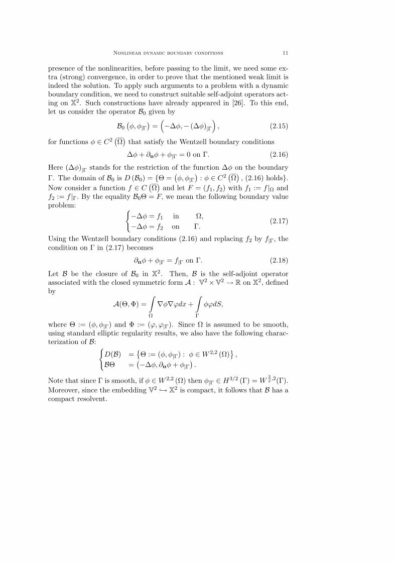
presence of the nonlinearities, before passing to the limit, we need some ex-tra (strong) convergence, in order to prove that the mentioned weak limit isindeed the solution. To apply such arguments to a problem with a dynamicboundary condition, we need to construct suitable self-adjoint operators act-ing on X2. Such constructions have already appeared in [26]. To this end,let us consider the operator B0 given by
B0φ,φ|Γ
=
−∆φ,− (∆φ)|Γ
, (2.15)
for functions φ ∈ C2Ω
that satisfy the Wentzell boundary conditions
∆φ + ∂nφ + φ|Γ = 0 on Γ. (2.16)
Here (∆φ)|Γ stands for the restriction of the function ∆φ on the boundaryΓ. The domain of B0 is D (B0) = Θ =
φ, φ|Γ
: φ ∈ C
2Ω
, (2.16) holds.
Now consider a function f ∈ CΩ
and let F = (f1, f2) with f1 := f |Ω and
f2 := f |Γ. By the equality B0Θ = F, we mean the following boundary valueproblem:
−∆φ = f1 in Ω,
−∆φ = f2 on Γ.(2.17)
Using the Wentzell boundary conditions (2.16) and replacing f2 by f|Γ, thecondition on Γ in (2.17) becomes
∂nφ + φ|Γ = f|Γ on Γ. (2.18)
Let B be the closure of B0 in X2. Then, B is the self-adjoint operatorassociated with the closed symmetric form A : V2×V2 → R on X2
, definedby
A(Θ, Φ) =
Ω
∇φ∇ϕdx +
Γ
φϕdS,
where Θ := (φ,φ|Γ) and Φ := (ϕ,ϕ|Γ). Since Ω is assumed to be smooth,using standard elliptic regularity results, we also have the following charac-terization of B:
D(B) =Θ := (φ,φ|Γ) : φ ∈ W
2,2 (Ω)
,
BΘ =−∆φ, ∂nφ + φ|Γ
.
Note that since Γ is smooth, if φ ∈ W2,2 (Ω) then φ|Γ ∈ H
3/2 (Γ) = W32 ,2(Γ).
Moreover, since the embedding V2→ X2 is compact, it follows that B has a
compact resolvent.

12 Ciprian G. Gal and Mahamadi Warma,
Therefore, for i ∈ N, we take a complete system of eigenfunctions Φi =(φi,ψi) of the problem BΦi = λiΦi in X2 with Θi ∈ D (B) ∩ C
2Ω
. Ac-
cording to the general spectral theory, the eigenvalues λi ∈ (0, +∞) can beincreasingly ordered and counted according to their multiplicities in order toform a real divergent sequence. Moreover, the respective eigenvectors turnout to form an orthogonal basis both in V2 and X2 and may be assumed tobe normalized in the norm of X2. At this point, we set the spaces
Kn = span Φ1, Φ2, ...,Φn , K∞ =∞
n=1
Kn.
Clearly, K∞ is a dense subspace of both V2 and D (B). Let Prn : X2 → Kn
be an orthogonal projection. For any n ∈ N, we look for functions of theform
Φ = Φn =n
i=1
di (t)Φi (2.19)
solving the approximate problem (Pn) that we will introduce below. Notethat in the definition of Φn, di (t) are sought to be suitably regular realvalued functions (i.e., di ∈ C
2 (0, T ) , i = 1, ..., n.). Note that from (2.19),we also have
φ = φn =n
i=1
di (t)φi, ψ = ψn =n
i=1
di (t)ψi.
As approximations for the initial data Φ0 = (φ0,ψ0), ψ0 = φ0|Γ, we takeΦn0 ∈ Vp, such that
limn→∞
Φn0 = Φ0 in X2,
since Vp is dense in X2. The problem that we must solve is given, for anyn ≥ 1, by (Pn): find Φn such that, for all Φ =
φ, ψ
∈ Kn,
∂tΦn, Φ
X2 +
PrnBpΦn, Φ
X2 +
PrnF (Φn) , Φ
X2 =
PrnG, Φ
X2 , (2.20)
and Φn (0) , Φ
X2 =
Φn0, Φ
X2 . (2.21)
Here, G =(g1, g2) and the operators Bp : D (Bp) → X2, F : D(F) ⊂ X2 → X2
are given, formally, by
Bp
φ
ψ
=
−∆pφ + |φ|p−2
φ
|∇ψ|p−2∂nφ
, (2.22)
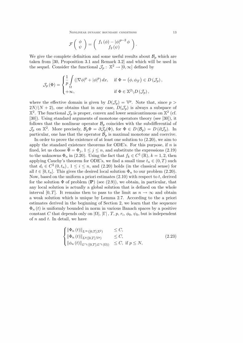
Nonlinear dynamic boundary conditions 13
F
φ
ψ
=
f1 (φ)− |φ|p−2
φ
f2 (ψ)
.
We give the complete definition and some useful results about Bp which aretaken from [30, Proposition 3.1 and Remark 3.2] and which will be used inthe sequel. Consider the functional Jp : X2 → [0,∞] defined by
Jp (Φ) =
1p
Ω
(|∇φ|p + |φ|p) dx, if Φ =φ,φ|Γ
∈ D (Jp) ,
+∞, if Φ ∈ X2\D (Jp) ,
where the effective domain is given by D(Jp) = Vp. Note that, since p >
2N/(N + 2), one obtains that in any case, D(Jp) is always a subspace ofX2. The functional Jp is proper, convex and lower semicontinuous on X2 (cf.[30]). Using standard arguments of monotone operators theory (see [30]), itfollows that the nonlinear operator Bp coincides with the subdifferential ofJp on X2. More precisely, BpΦ = ∂Jp(Φ), for Φ ∈ D (Bp) = D (∂Jp). Inparticular, one has that the operator Bp is maximal monotone and coercive.
In order to prove the existence of at least one solution to (2.20), we aim toapply the standard existence theorems for ODE’s. For this purpose, if n isfixed, let us choose Φ = Φj , 1 ≤ j ≤ n, and substitute the expressions (2.19)to the unknowns Φn in (2.20). Using the fact that fk ∈ C
1 (R), k = 1, 2, thenapplying Cauchy’s theorem for ODE’s, we find a small time tn ∈ (0, T ) suchthat di ∈ C
2 (0, tn) , 1 ≤ i ≤ n, and (2.20) holds (in the classical sense) forall t ∈ [0, tn]. This gives the desired local solution Φn to our problem (2.20).Now, based on the uniform a priori estimates (2.10) with respect to t, derivedfor the solution Φ of problem (P) (see (2.9)), we obtain, in particular, thatany local solution is actually a global solution that is defined on the wholeinterval [0, T ]. It remains then to pass to the limit as n → ∞ and obtaina weak solution which is unique by Lemma 2.7. According to the a prioriestimates derived in the beginning of Section 2, we learn that the sequenceΦn (t) is uniformly bounded in norm in various Banach spaces by a positiveconstant C that depends only on |Ω|, |Γ| , T, p, ri, φ0, ψ0, but is independentof n and t. In detail, we have
Φn (t)L∞([0,T ];X2) ≤ C,
Φn (t)Lp([0,T ];Vp) ≤ C,
φn (t)Lr1 ([0,T ];Lr1 (Ω)) ≤ C, if p ≤ N,
(2.23)
14 Ciprian G. Gal and Mahamadi Warma,
andφn (t)Lp([0,T ];C(Ω)) ≤ C, if p > N.
On account of the uniform bounds in (2.23), we can get further uniformbounds for Prn BpΦn and PrnF (Φn). Indeed, by the boundedness of theprojection Prn, we immediately deduce that
PrnBpΦn (t)(Vp)∗ = supΦVp≤1
BpΦn (t) , PrnΦ
X2
≤ Φn (t)p−1Vp ,
so thatPrnBpΦn (t)Lq([0,T ];(Vp)∗) ≤ C, (2.24)
where we may identify the dual space of Vp, (Vp)∗ with a closed subspace ofW−1,q (Ω)⊕W
1/p−1,q (Γ) , q = p/(p− 1) is the conjugate exponent of p.Let us now focus on the case p ≤ N . On account of assumptions (2.7) and
the last two uniform bounds of (2.23), it is not difficult to show that f1 (φn),f2 (ψn) are uniformly bounded (with respect to n) in L
r1([0, T ] ;Lr
1 (Ω))
and Lr2([0, T ] ;Lr
2 (Γ)), respectively, where r
i are conjugate to ri. Since,
Lri([0, T ] ;Lr
i) → L
ri([0, T ] ; (Vp)∗), it follows that f1 (φn) and f2 (ψn) are
uniformly bounded in Lr1([0, T ] ; (Vp)∗) and L
r2([0, T ] ; (Vp)∗), respectively.
When p > N, the same is true except that we need to take ri = q, for
all i = 1, 2. Finally, we need a uniform bound on the derivatives. Bycomparison, from equation (2.20), we have that ∂tΦn is uniformly boundedin L
s ([0, T ] ; (Vp)∗) , with s = min(q, r1, r2) > 1. It is now obvious that
∂tΦn + PrnBpΦn + PrnF (Φn) = PrnG
holds as an equality in Ls ([0, T ] ; (Vp)∗).
From this point on, all convergence relations will be intended to hold up tothe extraction of suitable subsequences, generally not relabelled. Thus, weobserve that weak and weak star compactness results applied to the abovesequences Φn = (φn,ψn) entail that there exists a function Φ = (φ,ψ) suchthat as n → +∞, the following properties hold:
Φn → Φ weakly star in L∞
[0, T ] ; X2, (2.25)
Φn → Φ weakly in Lp ([0, T ] ; Vp) ,
(∂tφn, ∂tψn) → ∂tΦ weakly in Ls ([0, T ] ; (Vp)∗) . (2.26)
Using the fact that Vp→ X2 =
X2
∗→ (Vp)∗, then, standard interpolation
and compact embedding results for vector valued functions (see, e.g., [24,

Nonlinear dynamic boundary conditions 15
Lemma 8]) ensure that
Φn → Φ strongly in C[0, T ] ;
(Vp)∗ , X2
κ
, (2.27)
Φn → Φ strongly in Lp[0, T ] ; X2
, (2.28)
where (·, ·)κ denotes the interpolation space. Clearly, Φ ∈ C ([0, T ] ; (Vp)∗).Also by refining in (2.28), φn converges to φ a.e. in Ω × (0, T ) and ψn
converges to ψ a.e. in Γ × (0, T ) , respectively. Then, by means of knownresults of measure theory (see, e.g., [42, Lemma 8.3 ]), the continuity of fk,
k = 1, 2, and the convergence of (2.28) easily imply that f1 (φn) convergesweakly to f1 (φ) in L
r1(Ω×(0, T )), and thus, weakly star in L
s ([0, T ] ; (Vp)∗).Moreover, f2 (ψn) converges weakly to f2 (ψ) in L
r2(Γ × (0, T )), and thus,
weakly star in Ls ([0, T ] ; (Vp)∗). Since the orthogonal projection Ln :=
(I − Prn) to Prn has the known property that LnΦi → 0 in Vp (as n →∞)for each 1 ≤ i ≤ n, it is now an easy task to show that
PrnF (Φn) → F (Φ) weakly star in Ls ([0, T ] ; (Vp)∗) . (2.29)
On the other hand, on account of (2.23), (2.27)-(2.28) and exploiting suitablemonotonicity arguments, we show that Prn BpΦn converges weakly star toBpΦ in L
s ([0, T ] ; (Vp)∗). Indeed, since Bp = LnBp + Prn Bp, it only sufficesto show that BpΦn converges weakly star to BpΦ in L
s ([0, T ] ; (Vp)∗) . Weargue as follows. By (2.24), the function BpΦn is uniformly bounded inL
q ([0, T ] ; (Vp)∗). Hence, we can choose a subsequence of Φn which we alsodenote by Φn such that
BpΦn → Ξ weakly star in Lq ([0, T ] ; (Vp)∗) , (2.30)
and thus weakly star in Ls ([0, T ] ; (Vp)∗) , since s ≤ q. Exploiting the above
converge properties (2.26), (2.29), (2.30), and passing to the limit in equation(2.20), we have that
∂tΦ + Ξ + F (Φ) = G (2.31)
holds as an equality in Ls ([0, T ] ; (Vp)∗). Let us now prove the equality
Ξ = BpΦ. To this end, consider the integral
T
0
BpΦn − BpΨ, Φn −ΨX2 dt =: δn, (2.32)

16 Ciprian G. Gal and Mahamadi Warma,
where Φn, Ψ ∈ Lp ([0, T ] ; Vp). Obviously, δn ≥ 0 since Bp is maximal
monotone on X2. Moreover, the following integration by parts formula holds:t
0
∂tΦ1, Φ2X2+Φ1, ∂tΦ2X2
ds = Φ1 (t) ,Φ2 (t)X2−Φ1 (0) ,Φ2 (0)X2 ,
(2.33)for all t ∈ [0, T ] , and Φk ∈ L
p ([0, T ] ; Vp) , ∂tΦk ∈ Lq ([0, T ] ; (Vp)∗) , k = 1, 2.
Such formulas can be easily obtained by approximating Φk by a sequence ofmollifiers (in time) (Φk)h ∈ C
1 ([0, T ] ; Vp), then followed by passage to thelimit in h. Take Φ1 = Φ2 = Φn in (2.33) (note that, within the approximationscheme (2.20), the functions Φn already belong to C
1 ((0, T ) ; Vp) since di ∈C
1 (0, T ), for all i). We havet
0
BpΦn, ΦnX2 ds = −t
0
[F (Φn) , ΦnX2 − G,ΦnX2 ] ds (2.34)
+12Φn (0)2X2 −
12Φn (t)2X2 .
Therefore, by (2.32) and (2.34),
δn =12Φn (0)2X2 −
12Φn (t)2X2 −
t
0
[F (Φn) , ΦnX2 − G,ΦnX2 ] ds
(2.35)
−t
0
BpΦn, ΨX2 + BpΨ, Φn −ΨX2
ds.
Following known results of measure theory, (2.27), (2.28) also yield thatΦn (t) → Φ (t) in the weak topology of X2 and Φ (t) is a weakly continuousfunction from [0, T ] to X2. Besides,
Φ (t)2X2 ≤ limn
inf Φn (t)2X2 (2.36)
and Φn (0) → Φ (0) strongly in X2 (which follows by construction). Ex-ploiting (2.36), the above converge properties for F (Φn) , BpΦn (see (2.25)-(2.30)), and passing to the limit as n → +∞ in (2.35), we get
− 12Φ (0)2X2 +
12Φ (t)2X2 +
t
0
[F (Φ) , ΦX2 − G, ΦX2 ] ds (2.37)

Nonlinear dynamic boundary conditions 17
≤ −t
0
BpΨ, Φ−ΨX2 + Ξ, ΨX2
ds.
Now, let us take Φ1 = Φ2 = Φ in (2.33) and exploit the equality (2.31) onceagain. We deduce
−t
0
Ξ,ΦX2 ds =t
0
[F (Φ) , ΦX2 − G,ΦX2 ] ds (2.38)
+12Φ (t)2X2 −
12Φ (0)2X2 .
Adding the relations (2.37) and (2.38) together, it is not difficult to see thatwe obtain the following inequality:
t
0
Ξ− BpΨ, Φ−ΨX2 ds ≥ 0, (2.39)
for all Ψ ∈ Lp ([0, T ] ; Vp). Finally, by setting Ψ = Φ + εΘ, with ε ∈ (0, 1],
Θ ∈ Lp ([0, T ] ; Vp) in (2.39) and dividing by ε, and arguing in a standard
way (we employ Lebesgue’s theorem and pass to the limit as ε → 0), it isnot difficult to realize that
t
0
Ξ− BpΦ, ΘX2 ds = 0, ∀Θ ∈ Lp ([0, T ] ; Vp) .
This proves that Ξ = BpΦ in Lq ([0, T ] ; (Vp)∗) and since weak limits are
unique,BpΦn → BpΦ weakly star in L
q ([0, T ] ; (Vp)∗) . (2.40)
By means of the above convergence properties (2.26), (2.29) and (2.40), wecan readily pass to the limit in (2.20) and find that (φ (t) ,ψ (t)) solves (2.9).
Finally, it is left to show that ψ (0) = ψ0 and φ (0) = φ0. To this end,choose a test function Π ∈ C
1 ([0, T ] ; Vp) with Π (T ) = 0, and compare theresults of taking Φ = Π in (2.20) and (2.31), respectively. Passing to thelimit once again by using the above convergence properties of the solutions(φn, ψn), we easily obtain our desired conclusion. The uniqueness of theweak solution follows from Lemma 2.7 below. The proof of the theorem isfinished.

18 Ciprian G. Gal and Mahamadi Warma,
It remains to verify the uniqueness of the solution and the Lipschitz con-tinuity with respect to the initial data (φ0,ψ0) ∈ X2.
Lemma 2.7. Let the assumptions above hold and let the functions (φ1,ψ1)and (φ2,ψ2) be two solutions of problem (2.9). Set
φ (t) , ψ (t)
:= (φ1 (t)− φ2 (t) ,ψ1 (t)− ψ2 (t)) .
Then, the following estimate holds:φ (t)
2
L2(Ω)+
ψ (t)2
L2(Γ)≤ Le
Ltφ (0)
2
L2(Ω)+
ψ (0)2
L2(Γ)
, (2.41)
for all t ≥ 0, where the positive constant L is independent of t, but dependson the norm of the initial data (φi (0) ,ψi (0)) , i = 1, 2, in X2.
Proof. We work within the Galerkin discretization scheme introduced above.With reference to the proof of Theorem 2.6, let Φn (t) = (φn (t) ,ψn (t)) andΦm (t) = (φm (t) , ψm (t)) be two solutions of problem Pn (see (2.20)-(2.21))and Pm, corresponding to the initial data Prn Φ1 (0) and Prm Φ2 (0) , andthe same source term G, respectively. First notice that
Φn (t) , Φm (t) ∈ C1 ((0, T ) ; Vp) ,
for all m,n ≥ 1; set Φmn (t) := Φm (t)−Φn (t). Then, the following equationis satisfied
∂tφmn,φ
2+
∂tψmn,ψ
2+
BpΦm − BpΦn, Φ
X2 (2.42)
+F (Φm)− F (Φn) ,Φ
X2
= 0,
for all Φ =φ,ψ
∈ Km ∩Kn, with the initial data Φmn (0) = Prm Φ2 (0)−
Prn Φ1 (0).Taking Φ = Φmn (t), i.e., φ = φmn (t) and ψ = ψmn, respectively, the
equality ( 2.42) then yields12
d
dt
φmn (t)2L2(Ω) + ψmn (t)2L2(Γ)
(2.43)
+
Ω
|∇φm|p−2∇φm − |∇φn|p−2∇φn
·∇φmndx
= −f1 (φm)− f1 (φn) , φmn (t)2 − f2 (ψm)− f2 (ψn) ,ψmn (t)2,Γ .
Now, it is readily seen that assumption (2.6) also implies that
fi (y) ≥ −Mi,∀y ∈ R, (2.44)

Nonlinear dynamic boundary conditions 19
for some Mi > 0, i = 1, 2. Using now the obvious inequality|a|p−2
a− |b|p−2b
(a− b) ≥ υ
|a|p−2 + |b|p−2
|a− b|2 ,
which holds for some positive constant υ, and for all a, b ∈ RN and p ∈[p0,+∞) ∩ (1, +∞) (see, e.g., [30, Lemma 2.13]), we can control the secondterm on the left-hand side of (2.43). Using (2.44) to control the right-handside, we deduce
12
d
dt
(φmn (t) ,ψmn (t))2X2
+ υ
Ω
|∇φm|p−2 + |∇φn|p−2
|∇φmn|2 dx
(2.45)
≤ c (φmn (t) ,ψmn (t))2X2 , ∀t ≥ 0.
Integrating this inequality from 0 to t and passing to the limit as m,n →∞,we immediately obtain the claim (2.41), owing to Gronwall’s inequality. Letus choose Φ2 (0) = Φ1 (0). It is clear then, from (2.45), that (φn,ψn) isalso a Cauchy sequence in X2 and, therefore, (φ (t) ,ψ (t)) ∈ C
[0, T ] ; X2
.
The proof of Lemma 2.7 is now finished. Theorem 2.8. Let the assumptions of Theorem 2.6 be satisfied. The semi-group St is
X2
, Vp-bounded for t > 0, i.e., for any (φ0, ψ0) bounded in X2,
the solution (φ (t) ,ψ (t)) = St (φ0, ψ0) is bounded in Vp, for all t > 0. Moreprecisely, the following estimate holds:
(φ (t) ,ψ (t))pVp + φ (t)r1
Lr1 (Ω) (2.46)
≤ c0t−1 (φ (0) ,ψ (0))2X2 + c0
1 + g1q
Lr1 (Ω)+ g2q
Lr2(Γ)
,
for all t > 0, where c0 > 0 is independent of time and initial data. Inparticular, the set (φ (t) ,ψ (t)) ∈ Vp : t ≥ 1 is precompact in X2.
Proof. Take Φ = ∂tΦn = (∂tφn, ∂tψn) in (2.20) and recall (1.6). We have
∂tφn (t)2L2(Ω) + ∂tψn (t)2L2(Γ) +d
dt[EΩ (φn (t)) + EΓ (ψn (t))] = 0, (2.47)
where the energy functionals EΩ (φ), EΓ (ψ) are defined in (1.3)-(1.4). Recallthat F
i = fi, i = 1, 2. From the assumptions (2.6)-(2.7), it is easy to check
that these functions also satisfy
η1 |y|r1 − ν 1 ≤ F1 (y) ≤ ν1 |y|r1 + ν 1, (2.48)
−ν 2 ≤ F2 (y) ≤ ν2 |y|r2 + ν 2,

20 Ciprian G. Gal and Mahamadi Warma,
while this fact implies that for all t ≥ 0,
c
φ (t)r1
Lr1 (Ω) − |Ω|ν 1 − S(Γ)ν 2≤
Ω
F1 (φ (t)) dx +
Ω
F2 (ψ (t)) dS
(2.49)
≤ c
φ (t)r1
Lr1 (Ω) + ψ (t)r2Lr2 (Γ)
+ cν 1|Ω|+ ν 2S(Γ)
.
Let us now multiply (2.47) by t and integrate the resulting relation over(0, t). We deduce
t [EΩ (φn (t)) + EΓ (ψn (t))] +t
0
s
∂tφn (s)2L2(Ω) + ∂tψn (s)2L2(Γ)
ds
(2.50)
=t
0
(EΩ (φn (s)) + EΓ (ψn (s))) ds,
for all t ≥ 0. Using estimates (2.10), (2.49) and exploiting the embeddingsW
1,p (Ω) → Lr1 (Ω) , W
1,p (Ω) → Lr2 (Γ) , we conclude that the right-hand
side of (2.50) is bounded from above, that is,
t
0
(EΩ (φn (s)) + EΓ (ψn (s))) ds (2.51)
≤ c (φ (0) ,ψ (0))2X2 + ct
1 + g1q
Lr1 (Ω)+ g2q
Lr2 (Γ)
,
for all t ≥ 0. Combining (2.50) with (2.51), we obtain the following inequal-ity:
EΩ (φn (t)) + EΓ (ψn (t)) + t−1
t
0
s
∂tφn (s)2L2(Ω) + ∂tψn (s)2L2(Γ)
ds
(2.52)
≤ ct−1 (φ (0) ,ψ (0))2X2 + c
1 + g1q
Lr1 (Ω)+ g2q
Lr2 (Γ)
,

Nonlinear dynamic boundary conditions 21
for all t > 0. From (2.52), it is readily seen, on account of (2.49), that
(φn (t) ,ψn (t))pVp + φn (t)r1
Lr1 (Ω) (2.53)
≤ ct−1 (φ (0) ,ψ (0))2X2 + c
1 + g1q
Lr1 (Ω)+ g2q
Lr2(Γ)
,
for all t > 0. Passing to the limit as n → +∞ over a subsequence Φn (t) =(φn (t) ,ψn (t)) which is weakly star convergent in L
∞ ([ε, T ] ; Vp ∩ Lr1 (Ω))
and weakly in W1,2
[ε, T ] ; X2
, for any ε > 0, the claim (2.46) follows
immediately from (2.53), owing to the lower semicontinuity of the norms.Moreover, we have
∂tΦ ∈ W1,2
[ε, T ] ; X2
, (2.54)
for any ε > 0. The relative compactness of any trajectory (φ (t) ,ψ (t)) ,
t ≥ 1 is a straightforward consequence of (2.46) and the compact embeddingof Vp into X2. The proof is finished. Remark 2.9. Because of the regularity in (2.54), the function ∂tΦ (t) , t ∈[ε, T ] (for any ε > 0), can be now viewed as a pair and, effectively, thesolution (φ (t) ,ψ (t)) of problem P satisfies the following ”improved” weakformulation:
∂tφ (t) ,σ2 + ∂tψ (t) ,σ2,Γ +|∇φ (t)|p−2∇φ (t) ,∇σ
2
+ f1 (φ (t)) ,σ2 +f2 (ψ (t)) ,σ|Γ
2,Γ
= g1,σ2 +g2,σ|Γ
2,Γ
,
for all t ≥ ε > 0 and all Ξ =σ,σ|Γ
∈ Vp
.
Remark 2.10. Theorem 2.6 still remains true if the quasilinear operators∆pφ and |∇φ|p−2
∂nφ from (1.2) and (1.7) are replaced by the operatorsdiv (a (|∇φ|)∇φ) and b (x) a (|∇φ|) ∂nφ, where b ∈ L
∞ (Γ) , b ≥ b0 > 0and a ∈ C
1RN
, R
is a monotone nondecreasing function that satisfies thefollowing assumptions:
|a (y)| ≤ c1(1 + |y|p−2), ∀y ∈ RN
,
a (y) |y|2 ≥ c2 |y|p , ∀y ∈ RN,
for some positive constants c1, c2.
3. Global attractors
Before we state our main results of this section, we recall some basicdefinitions about global attractors.

22 Ciprian G. Gal and Mahamadi Warma,
Definition 3.1. Let Stt≥0 be a semigroup on a Banach space X and Z
be a metric space. A set A ⊂ X ∩ Z, which is invariant (that is, StA = A,
∀t ≥ 0), closed in X, compact in Z and attracts bounded subsets of X in thetopology of Z is called an (X, Z) -attractor. More precisely, for any boundedsubset B ⊂ X, we have
limt→+∞
distZ (StB,A) = 0, (3.1)
where distZ denotes the Hausdorff semidistance with respect to the metric ofZ, which is defined as
distZ (X, Y ) := supx∈X
infy∈Y
x− yZ .
Definition 3.2. A bounded subset B0 ⊂ Z is called an (X,Z)-bounded ab-sorbing set, if for any bounded subset B ⊂ X, there exists a time t
# =t# (B) , such that StB ⊂ B0, for any t ≥ t
#.
Next, we derive stronger global a priori estimates for the solutions ofproblem (P) in the space X2 (compare with Proposition 2.5). These a prioriestimates are necessary for the study of the asymptotic behavior of ourproblem.
Proposition 3.3. Suppose that fi ∈ Ni (p, ri) if p ≥ 2 and fi ∈ Ni (p, ri) ifp ∈ (p0, 2)∩ (1, +∞), for each i = 1, 2, where by fi ∈ Ni (p, ri), we mean thefollowing: fi satisfies (1.4) and
η1 |y|2 − ν
1 ≤ f1 (y) y ≤ ν1 |y|r1 + ν
1,
η2 |y|2 − ν2 ≤ f2 (y) y ≤ ν2 |y|r2 + ν
2,
(3.2)
for some ηi, νi > 0, νi ≥ 0, with r1, r2 as in Definition 2.1. Let g1 ∈ L
r1 (Ω) ,
g2 ∈ Lr2 (Γ), where r
i are conjugate to ri. Let (φ (t) ,ψ (t)) be a weak solution
of (2.5) (i.e, satisfies (2.9)). Then, the following estimate holds:
(φ (t) ,ψ (t))2X2 +t
0
φ (s)p
W 1,p(Ω) + ψ (s)pW 1−1/p,p(Γ)
ds (3.3)
≤ c
(φ (0) , ψ (0))2X2
e−ρt + c
1 + g1q
Lr1 (Ω)+ g2q
Lr2(Γ)
,
for all t ≥ 0, where the positive constants c, ρ are independent of time andinitial data.

Nonlinear dynamic boundary conditions 23
Proof. We divide the proof of (3.3) into two parts. First, we show (3.3) for2 ≤ p ≤ N . The case p > N follows similarly with minor modifications.Using the facts that W
1,p (Ω) → L2 (Ω) and W
1−1/p,p (Γ) → L2 (Γ) for
p ∈ [p0, +∞) ∩ (1, +∞), we can rewrite (2.13) as follows:12
d
dt
φ (t)2L2(Ω) + ψ (t)2L2(Γ)
+
c
4
φ (t)p
L2(Ω) + ψ (t)pL2(Γ)
(3.4)
+c
2φ (t)r1
Lr1 (Ω) +c
4
φ (t)p
W 1,p(Ω) + ψ (t)pW 1−1/p,p(Γ)
≤ c
1 + g1q
Lr1(Ω)+ g2q
Lr2 (Γ)
.
First from Young’s inequality, we notice that
φ(t)2L2(Ω) ≤ c
1 + φ(t)p
L2(Ω)
and ψ(t)2L2(Γ) ≤ c
1 + ψ(t)p
L2(Γ)
.
(3.5)Using (3.5), from (3.4), we deduce that
12
d
dt
φ (t)2L2(Ω) + ψ (t)2L2(Γ)
+
ρ
2
φ (t)2L2(Ω) + ψ (t)2L2(Γ)
(3.6)
+c
2φ (t)r1
Lr1 (Ω) +c
4
φ (t)p
W 1,p(Ω) + ψ (t)pW 1−1/p,p(Γ)
≤ c
1 + g1q
Lr1 (Ω)+ g2q
Lr2 (Γ)
,
for some positive constant ρ that depends only on p, c, Ω and Γ. Applying asuitable version of Gronwall’s inequality (see e.g., [31, Lemma 2.5]) to (3.6),we easily deduce estimate (3.3). In particular, we also have that
t
0
(φ (s) ,ψ (s))p
Vp + φ (s)r1Lr1(Ω)
ds (3.7)
≤ c
(φ (0) ,ψ (0))2X2
e−ρt + c
1 + g1q
Lr1 (Ω)+ g2q
Lr2 (Γ)
,
for all t ≥ 0.Let us now show (3.3) when p ∈ (p0, 2) ∩ (1,+∞). To this end, recall
(2.11). Exploiting the new assumptions (3.2), from (2.11), we deduce12
d
dt
φ (t)2L2(Ω) + ψ (t)2L2(Γ)
+ ∇φ (t)p
Lp(Ω) (3.8)
+ η1 φ (t)2L2(Ω) + η2 ψ (t)2L2(Γ)
≤ g1,φ (t)2 + g2,ψ (t)2,Γ + c.
24 Ciprian G. Gal and Mahamadi Warma,
Setting ρ = min (η1, η2) > 0, then using the embeddings W1,p (Ω) →
L2 (Ω) , L
2 (Ω) → Lp (Ω) (which, by Young’s inequality also imply that
|·|pLp(Ω) ≤ c(1 + |·|2Lp(Ω)), for some c > 0), we obtain
12
d
dt
φ (t)2L2(Ω) + ψ (t)2L2(Γ)
+ c φ (t)p
W 1,p(Ω) (3.9)
+ρ
2
φ (t)2L2(Ω) + ψ (t)2L2(Γ)
≤ g1,φ (t)2 + g2,ψ (t)2,Γ + c,
for all t ≥ 0. Finally, exploiting suitable Young inequalities in order tocontrol the terms on the right-hand side of (3.9) (see, e.g., (2.13)) and arguingas in (3.6)-(3.7), we obtain the desired inequality (3.3) for p < 2. The proofis finished.
Remark 3.4. Obviously, the result of Theorem 2.6 is still valid if fi ∈Ni (p, ri) , i = 1, 2, when p ∈ (p0, 2) ∩ (1, +∞), that is, we still have aunique weak solution under the new assumptions. Indeed, the global a prioriestimate (2.10) follows easily by integrating the inequality (3.9) over (0, t).
Theorem 3.5. Let the assumptions of Proposition 3.3 be satisfied. Endowthe Banach space Zp
r1 := Vp ∩ Lr1 (Ω) with the metric topology of Vp. Then
the solution semigroup Stt≥0 has aX2
, Zpr1
-bounded absorbing set. More
precisely, there is a positive constant C, depending only on the physical pa-rameters of the problem, such that for any bounded subset B ⊂ X2, thereexists a positive constant t
# = t# (BX2) such that
(φ (t) ,ψ (t))Vp + φ (t)Lr1 (Ω) ≤ C, (3.10)
for all t ≥ t#
.
Proof. First, we note that, setting
R0 := 2c(1 + g1q
Lr1 (Ω)+ g2q
Lr2 (Γ))
and
t# =
1ρ
ln2C (φ (0) ,ψ (0))2X2 /R0
in (3.3), we obtain that
(φ (t) ,ψ (t))X2 ≤ R0, for all t ≥ t#
. (3.11)

Nonlinear dynamic boundary conditions 25
Next, we showt+1
t
(φ (s) ,ψ (s))p
Vp + φ (s)r1Lr1 (Ω)
ds (3.12)
−t+1
t
g1,φ (s)2 + g2, ψ (s)2,Γ
ds
≤ C (R0) ,
for all t ≥ t#
, where the positive constant C (R0) depends only on R0, but isindependent of t and initial data. Indeed, integrating (2.12) from t to t + 1yields
φ(t + 1),ψ(t + 1)2X2 − φ(t), ψ(t)2X2 (3.13)
+ c
t+1
t∇φ(s)p
Lp(Ω) + φ(s)r1Lr1 (Ω)
ds
≤ t+1
t
g1, φ(s)2 + g2,ψ(s)2,Γ + c
ds.
Using the fact that Lr1(Ω) → L
p(Ω) and Young’s inequality, we have, forevery ε > 0, that
φ(t)pLp(Ω) ≤ cφ(t)p
Lr1 (Ω) ≤ cε− p
r1 φ(t)r1Lr1 (Ω) + ε
r1−pr1 . (3.14)
Using (3.14) and the fact that the norms uW 1,p(Ω), (u, u|Γ)Vp are equiv-alent and recalling (3.11), from (3.13), we obtainUsing (3.14) and the factthat the norms uW 1,p(Ω), (u, u|Γ)Vp are equivalent and recalling (3.11),from (3.13), we obtain
t+1
t
(φ (s) ,ψ (s))p
Vp + φ (s)r1Lr1 (Ω)
ds
−t+1
t
g1,φ (s)2 + g2, ψ (s)2,Γ
≤ c + φ(t),ψ(t)2X2 ≤ C (R0) ,
for all t ≥ t#
. This completes the proof of (3.12).

26 Ciprian G. Gal and Mahamadi Warma,
Taking now σ = ∂tφ (t) and σ|Γ = ∂tψ (t) in (2.9), using (1.6) and recallingRemark 2.9, we deduce that
∂tφ (t)2L2(Ω) + ∂tψ (t)2L2(Γ) +d
dt[EΩ (φ (t)) + EΓ (ψ (t))] = 0, (3.15)
for all t ≥ t#. Recall that F
i = fi, i = 1, 2 satisfy (2.48) and estimate
(2.49) holds for any weak solution (φ (t) , ψ (t)) of (P). Applying now theuniform Gronwall’s lemma (see e.g., [44, Chapter 3, Lemma 1.1]) to (3.15),and employing the estimates (3.12), (2.49) once more, we can find anothertime t
∗ ≥ t# ≥ 1, such that the following inequality holds:
EΩ (φ (t)) + EΓ (ψ (t)) ≤ C (R0) , ∀t ≥ t∗, (3.16)
where the positive constant C (R0) depends on C (R0) , but is independentof time and initial data. Estimate (3.10) follows now immediately, thanksto (2.49)-(3.16), since g1 ∈ L
r1 (Ω), g2 ∈ Lr2 (Γ). The proof is finished.
Remark 3.6. It follows from (3.10) that the semigroup Stt≥0 always pos-sesses a
X2
, C(Ω)-bounded absorbing set if p > N or N = 1, since then
Vp→ C
Ω
, where we identify each function u ∈ C(Ω) with U = (u, u|Γ).
However, if p ≤ N , this is not always so. We will show that if we imposeadditional assumptions on the nonlinearities fi, i = 1, 2, then we obtain thatthe semigroup Stt≥0 also possesses a
X2
, X∞-bounded absorbing set if
p ≤ N . This issue is investigated below.
Assuming that the external forces gi are bounded, we have the followingresult which may be of interest on its own.
Theorem 3.7. Let p ∈ [p0,+∞)∩(1, +∞) and assume now that g1 ∈ L∞ (Ω)
and g2 ∈ L∞ (Γ) . Suppose that
fi (y) y ≥ Ci |y|2+β − Ci |y| , ∀y ∈ R, (3.17)
for some β > 0, Ci > 0, Ci ≥ 0, i = 1, 2. The following estimate holds for
the (weak) solutions of problem (P):
(φ (t) ,ψ (t))X∞ ≤ c + c0t−1/β
, for all t > 0, (3.18)
where the constants c, c0 > 0 are independent of time and initial data,and can be computed explicitly in terms of the structural parameters of theproblem.
Proof. Estimate (3.18) can be justified by means of the approximation pro-cedure devised in the proof of Theorem 2.6. Therefore, we proceed formally

Nonlinear dynamic boundary conditions 27
(note that di ∈ C2 (0, T ) in (2.19), therefore we can differentiate the equa-
tion with respect to time). We employ the weak formulation (2.9) of problem(2.5) once again. Let s > 1 and define the function
Ψs (t) =|φ (t)|s−2
φ (t) , |ψ (t)|s−2ψ (t)
. (3.19)
Taking σ = |φ|s−2φ, σ|Γ = |ψ|s−2
ψ in (2.9), and setting Θ(t) := (φ(t),ψ(t))and G := (g1, g2), we obtain
1s
d
dtΘ (t)s
Xs + (s− 1)
Ω
|φ (t)|s−2 |∇φ (t)|p dx (3.20)
+
Ω
|φ (t)|s−2f1 (φ)φ (t) dx +
Γ
|ψ (t)|s−2f2 (ψ)ψ (t) dS = G,Ψs (t)X2 .
By (3.17), we can control the last two integral terms on the left-hand sideof (3.20) as follows:
Ω
|φ (t)|s−2f1 (φ)φ (t) dx +
Γ
|ψ (t)|s−2f2 (ψ)ψ (t) dS (3.21)
≥C1 φ (t)s+β
Ls+β(Ω)+ C2 ψ (t)s+β
Ls+β(Γ)
−C1 φ (t)s−1
Ls−1(Ω) + C2 ψ (t)s−1
Ls−1(Γ)
.
Using now Holder’s inequality with exponents (∞, 1) in order to estimatethe term on the right-hand side of (3.20) and employing (3.21), we deducethat
1s
d
dtΘ (t)s
Xs + c Θ (t)s+βXs+β ≤ (GX∞ + c) Θ (t)s−1
Xs−1 (3.22)
where, from now on, c will denote a positive constant, independent of time,initial data and s, and which may take on different values, sometimes evenin the same line. Let us now estimate the Xs and Xs−1-norms of the solutionΘ (t) , using Holder’s inequality with exponents ((s + β) /s, (s + β) /β) and(s/ (s− 1) , s), respectively. We get
Θ (t)s−1Xs−1 ≤ Θ (t)s−1
Xs
µ
Ω
1/s
andΘ (t)s
Xs ≤ Θ (t)sXs+β
µ
Ω
β/(s+β),
28 Ciprian G. Gal and Mahamadi Warma,
whereµ
Ω
=
Ω
dx +
Γ
dS = |Ω|+ S(Γ).
Inserting the above inequalities in (3.22), and observing that1s
d
dtΘ (t)s
Xs = Θ (t)s−1Xs−1
d
dtΘ (t)Xs ,
from (3.22), we deduce thatd
dtΘ (t)Xs + c
µ
Ω
−β/s Θ (t)1+βXs ≤ (G (x)X∞ + c)
µ
Ω
1/s.
(3.23)Setting now ζ1 := c infs≥2
µ
Ω
−β/s> 0 and
ζ2 := sups≥2
(G (x)X∞ + c)µ
Ω
1/s,
and observing that ζ2 is finite, we haved
dtΘ (t)Xs + ζ1 Θ (t)1+β
Xs ≤ ζ2. (3.24)
Applying now a suitable version of Gronwall’s inequality (see, e.g., [44,Chapter 3, Lemma 5.1]) to (3.24), there are positive constants ζ3 and ζ4
depending only on ζ1, ζ2 (but, independent of time, initial data and s), suchthat
Θ (t)Xs ≤ ζ3 + ζ4t−1/β
, ∀t > 0. (3.25)Fixing now t > 0, and then passing to the limit in (3.25) as s → +∞, wereadily obtain the assertion (3.18). The proof is finished. Remark 3.8. Note that, for instance, if f1(y) = y
2(y − 1), then condition(3.17) is satisfied for some β > 0.
As a consequence of Theorem 3.7, we also obtain the following result.
Theorem 3.9. Let the assumptions of Theorem 3.7 be satisfied. If p ≤ N ,then the solution semigroup Stt≥0 has a
X2
, X∞-bounded absorbing set,
that is, there is a positive constant C (independent of initial data and time),such that for any bounded subset B ⊂ X2, there exists a positive constantt∗ = t
∗ (BX2) such that
(φ (t) ,ψ (t))X∞ ≤ C, for all t ≥ t∗. (3.26)
We continue with a smoothing estimate for (∂tφ, ∂tψ) of the solutions ofproblem (P).

Nonlinear dynamic boundary conditions 29
Theorem 3.10. Let p ≥ 2 and suppose that fi ∈ Ni (p, ri) , i = 1, 2. Forany set B ⊂ X2 of bounded initial data (φ0,ψ0) ∈ X2
, there exists a positiveconstant t
# = t# (B) > 0 such that
∂tφ (t)2L2(Ω) + ∂tψ (t)2L2(Γ) ≤ c0, ∀t ≥ t#
, ∀ (φ0,ψ0) ∈ B, (3.27)
where c0 > 0 is independent of time and initial data. In particular,
∂tφ (t)2L2(Ω) + ∂tψ (t)2L2(Γ) ≤ c01 + t
−1, ∀t > 0, ∀ (φ0,ψ0) ∈ B.
Proof. We will show (3.27) by a formal argument, since we can always employthe approximation procedure in Theorem 2.6. By differentiating the equa-tions of (2.9), formally, with respect to time, and denoting u (t) = ∂tφ (t) ,
v(t) = ∂tψ (t), we get
∂tu,σ2 +∂tv, σ|Γ
2,Γ
+|∇φ|p−2∇u,∇σ
2(3.28)
+ (p− 2)|∇φ|p−4 (∇φ ·∇u)∇φ,∇σ
2
+f1 (φ)u,σ
2+
f2 (ψ) v,σ|Γ
2,Γ
= 0,
∀σ ∈ Vp, a.e. in (0, +∞) , where v (t) := u (t)|Γ. Taking σ = u (t), σ|Γ = v (t)in (3.28), and using (2.44), we obtain
12
d
dt
u (t)2L2(Ω) + v (t)2L2(Γ)
+ (p− 1)
Ω|∇φ|p−2 |∇u|2 dx (3.29)
≤ M1 u (t)2L2(Ω) + M2 v (t)2L2(Γ) , ∀t ≥ 0.
Integrating this inequality over (s, t + 1) , t < s < t + 1, and setting M :=max (2M1, 2M2) , we deduce
u (t + 1)2L2(Ω) + v (t + 1)2L2(Γ) ≤ u (s)2L2(Ω) + v (s)2L2(Γ)
+ M
t+1
s
u (τ)2L2(Ω) + v (τ)2L2(Γ)
dτ,
and then integrating again between t and t + 1, so that
u (t + 1)2L2(Ω) + v (t + 1)2L2(Γ) (3.30)
≤ (1 + M)t+1
t
u (τ)2L2(Ω) + v (τ)2L2(Γ)
dτ, ∀t > 0.
30 Ciprian G. Gal and Mahamadi Warma,
On the other hand, integrating (3.15) over (t, t + 1), and employing (3.16)once more, it is not difficult to see that
t+1
t
u (τ)2L2(Ω) + v (τ)2L2(Γ)
dτ ≤ 2 C (R0) , ∀t ≥ t
∗, (3.31)
where C (R0) and t∗ are the constants defined in the proof of Theorem
3.5. The claim (3.27) follows now from (3.30) and (3.31). The proof isfinished.
From Theorems 3.4, 3.9, the compactness of the embeddings W1,p (Ω) →
L2 (Ω) , W
1−1/p,p (Γ) → L2 (Γ) , we state the main result of this paper.
Corollary 3.11. Let the assumptions of Proposition 3.3 be satisfied. Thenthe dynamical system
St, X2
generated by the problem (P) has a
X2
, Vpw-
global attractor Ap, that is, Ap is a compact subset of X2 (and weakly compactin Vp), which attracts all bounded subsets B of X2 with respect to the strongand weak topologies of X2 and Vp
w, respectively. More precisely,
limt→+∞
distY (StB,Ap) = 0, (3.32)
where Y is either Vpw or X2 endowed with the corresponding topology.
Proof. According to standard results on the existence of the global attractor(see, e.g., [7]), we need to check that the semigroup St is continuous in theX2-topology for every bounded subset of X2 and that St possesses a boundedin Vp, compact in X2 and weakly compact in Vp
, absorbing set. The firstis an immediate consequence of (2.41), whereas it follows from estimates(3.10), (3.26), that the C -ball in the space Vp is an absorbing set for thesemigroup St if C is large enough. Since this ball is obviously compact in theX2-topology and weakly compact in Vp, the existence of the
X2
, Vpw-global
attractor Ap follows from [7, 42, 44], while the convergence estimate (3.32)holds in the metrics of X2 and Vp
w, respectively.
Remark 3.12. Theorems 3.7, 3.9 and Corollary 3.11 also imply the follow-ing smoothing property:
St : X2→ Vp ∩ X∞, ∀t > 0. (3.33)
The global attractor Ap is a bounded subset of Vp ∩ X∞.

Nonlinear dynamic boundary conditions 31
Remark 3.13. Concerning the quasi-linear parabolic equations (1.2), wecan also handle dynamic boundary conditions that involve surface diffusion:
∂tφ−∆m,Γφ + |∇φ|p−2∂nφ + f2 (φ) = g2, on Γ× (0, +∞), (3.34)
where ∆m,Γ is defined as the generalized m -Laplace-Beltrami operator on Γ,that is,
∆m,Γφ = divΓ
|∇Γφ|m−2∇Γφ
, m ∈ (1, +∞) .
In particular, ∆2,Γ = ∆Γ is the well-known Laplace-Beltrami operator on Γ.Here, for any real valued function φ,
divΓφ =N−1
i=1
∂τiφ,
where ∂τiφ denotes the directional derivative of φ along the tangential direc-tions τi at each point on the boundary, whereas ∇Γφ =
∂τ1φ, ..., ∂τN−1φ
is
the tangential gradient at the boundary Γ. Under suitable assumptions onthe nonlinearities fk, k = 1, 2, and the other parameters of the problem, wecan also show that such problems (1.2), (3.34), (1.8) are well-posed in suit-able Banach spaces. They also possess global attractors and solutions havesimilar properties to the ones obtained above for problem (P).
Remark 3.14. Let us now recall the following functional E : Vp → R,
E (Φ) =
Ω
1p|∇φ|p + F1 (φ)− g1 (x)φ
dx (3.35)
+
Γ
[F2 (ψ)− g2 (x)ψ] dS,
for all Φ = (φ,ψ) ∈ Vp. If (φ,ψ) ∈ L∞ ((0, +∞) ; Vp) ∩ C
[0, +∞) ; X2
is
a weak solution of (P), then from (1.6) we haved
dtE((φ (t) , ψ (t))) = −∂tφ (t)2L2(Ω) − ∂tψ (t)2L2(Γ) , a.e. t > 0. (3.36)
It is worth mentioning that it would be interesting to show that the prob-lem (P) has a gradient structure, which would require to prove that E is acontinuous Lyapunov functional for the semigroup St. Note, from Theorem3.5, that the weak solution (φ (t) ,ψ (t)) of (2.5) is only a weak continuousfunction from (0,+∞) with values in Vp. However, we cannot show that(φ (t) ,ψ (t)) is norm continuous from (0,+∞) to Vp, unless we require ad-ditional assumptions on the nonlinearities f1, f2, such as, fi = fi1 + fi2,

32 Ciprian G. Gal and Mahamadi Warma,
i = 1, 2, with fi1 being monotone, satisfying similar growth conditions to fi
and with fi2 being a globally bounded Lipschitz perturbation. Thus, usingmonotone operator arguments (see, e.g., [47]; cf. also [4, Remark 3.6], [6]),we should be able to show that the connected global attractor Ap, associatedwith the dynamical system
St, X2
, coincides with the unstable manifold of
the set Σp of stationary points of (2.5), that is,
Ap = Wu (Σp) .
Let us also mention that it would also be interesting to investigate whetherany bounded trajectory of problem (P) converges to a single equilibrium thatis a stationary solution of (2.5). If fi, i = 1, 2, are monotone, it should bepossible to prove such a convergence via a suitable version of the Lojasiewicz-Simon inequality, proven in [9] for the quasilinear parabolic equations (1.2)with Dirichlet boundary conditions. We will come back to these issues in aforthcoming article.
Remark 3.15. In contrast to the case of non-degenerate parabolic PDE’s,not much seems to be known about the long term behavior of quasilinearparabolic equations in general. Indeed, even though we are dealing with aparabolic problem in bounded domain, the global attractor Ap seems to haveinfinite fractal dimension when p > 2. Indeed, it was observed in [14] forthe parabolic equation with p-Laplacian (1.2), subject to Dirichlet boundaryconditions, that the ε-Kolmogorov entropy of the attractor behaves as thepolynomial of 1/ε as ε → 0, thus resulting in an infinite dimensional at-tractor. However, their construction of the attractor is very special to theDirichlet condition, so that a new totally different argument must be usedwhen dealing with a dynamic boundary condition of the type (1.7). All theseissues will be the topics of future investigation.
References
[1] S. M. Allen and J. W. Cahn, A microscopic theory for the antiphase boundary motionand its application to antiphase domain coarsening, Acta Metallurgica, 27 (1979),1085–1095.
[2] M. Aida, M. Efendiev, and A. Yagi, Quasi-linear abstract parabolic evolution equationsand exponential attractors, Osaka J. Math., 42 (2005), 101–132.
[3] H. Amann and J. Escher, Strongly continuous dual semigroups, Ann. Mat. Pura Appl.,171 (1996), 41–62.
[4] G. Akagi and M. Otani, Evolution inclusions governed by the difference of two subd-ifferentials in reflexive Banach spaces, J. Differential Equations, 209 (2005), 392–415.
[5] E. DiBenedetto, “Degenerate Parabolic Equations,” Universitext, Springer-Verlag,New York, 1993.

Nonlinear dynamic boundary conditions 33
[6] H. Brezis, “Operateurs Maximaux Monotones et Semi-groupes de Contractions dansles Espaces de Hilbert,” North-Holland Math. Stud., vol. 5, North-Holland, Amster-dam, 1973.
[7] A. V. Babin and M. I. Vishik, “Attractors of Evolutions Equations,” North-Holland,Amsterdam, 1992.
[8] J. W. Cholewa and T. Dlotko, “Global Attractors in Abstract Parabolic Problems,”Cambridge University Press, 2000.
[9] R. Chill and A. Fiorenza, Convergence and decay rate to equiilibrium of boundedsolutions of quasi-linear parabolic equations, J. Differential Equations, 228 (2006),611–632.
[10] R. Chill, E. Fasangova, and J. Pruss, Convergence to steady states of solutions ofthe Cahn-Hilliard and Caginalp equations with dynamic boundary conditions, Math.Nachr., 13 (2006), 1448–1462.
[11] A. N. Carvalho and C. B. Gentile, Asymptotic behavior of nonlinear parabolic equa-tions with monotone principal part, J. Math. Anal. Appl., 280 (2003), 252–272.
[12] J. Crank, “The mathematics of Diffusion,” Second edition, Clarendon Press, Oxford,1975.
[13] I. Chueshov and B. Schmalfuss, Qualitative behavior of a class of stochastic parabolicPDEs with dynamical boundary conditions, Discrete Contin. Dyn. Syst., 18 (2007),315–338.
[14] M. A. Efendiev and M. Otani, Infinite-dimensional attractors for evolution equationswith p-Laplacian and their Kolmogorov entropy, Diff. Int. Eq., 20 (2007), 1201–1209.
[15] J. Escher, Quasilinear parabolic systems with dynamical boundary conditions, Comm.Partial Differential Equations, 18 (1993), 1309–1364.
[16] J. Escher, On quasilinear fully parabolic boundary value problems, Differential IntegralEquations, 7 (1994), 1325–1343.
[17] A. Favini, G. Ruiz Goldstein, J. A. Goldstein, and S. Romanelli, The heat equationwith general Wentzell boundary conditions, J. Evol. Equations, 2 (2002), 1–19.
[18] A. Favini, G. Ruiz Goldstein, J. A. Goldstein, and S. Romanelli, The heat equationwith nonlinear general Wentzell boundary condition, Adv. Differential Equations, 11(2006), 481–510.
[19] M. Fila and P. Quittner, Large time behavior of solutions of a semilinear parabolicequation with a nonlinear dynamical boundary condition, Topics in nonlinear analysis,251–272, Nonlinear Differential Equations Appl., 35, Birkhauser, Basel, 1999.
[20] H. P. Fischer, Ph. Maass, and W. Dieterich, Novel surface modes of spinodal decom-position, Phys. Rev. Letters, 79 (1997), 893–896.
[21] H. P. Fischer, Ph. Maass, and W. Dieterich, Diverging time and length scales ofspinodal decomposition modes in thin flows, Europhys. Letters, 62 (1998), 49–54.
[22] H.P. Fischer, J. Reinhard, W. Dieterich, J.-F. Gouyet, P. Maass, A. Majhofer, andD. Reinel, Time-dependent density functional theory and the kinetics of lattice gassystems in contact with a wall, J. Chem. Phys., 108 (1998), 3028–3037.
[23] Z. H. Fan and C. K. Zhong, Attractors for parabolic equations with dynamic boundaryconditions, Nonlinear Anal., 68 (2008), 1723–1732.
[24] C. G. Gal, Global well-posedness for a non-isothermal Cahn-Hilliard model with dy-namic boundary conditions, Adv. Differential Equations, 12 (2007), 12–45.

34 Ciprian G. Gal and Mahamadi Warma,
[25] C. G. Gal, Well-posedness and long time behavior of the non-isothermal viscous Cahn-Hilliard model with dynamic boundary conditions, Dynamics of Partial DifferentialEquations, 5 (2008), 39–67.
[26] C. G. Gal, G. R. Goldstein, J. A. Goldstein, S. Romanelli, and M. Warma, Fredholmalternative, semilinear elliptic problems and Wentzell boundary conditions, preprint.
[27] C. G. Gal and M. Grasselli, The non-isothermal Allen-Cahn equation with dynamicboundary conditions, Discrete and Contin. Dyn. Syst., 12 (2008), 1009–1040.
[28] C. G. Gal and M. Grasselli, On the asymptotic behavior for the Caginalp systemwith dynamic boundary conditions, Communications in Pure and Applied Analysis, 8(2009), 689–710.
[29] C. G. Gal and A. Miranville, Uniform global attractors for non-isothermal Cahn-Hilliard equations with dynamic boundary conditions, Nonlinear Anal. Series B: RealWorld Applications, 10 (2009), 1738–1766.
[30] C. G. Gal and M. Warma, Nonlinear elliptic boundary value problems at resonancewith nonlinear Wentzell-Robin type boundary conditions, Preprint.
[31] C. Giorgi, M. Grasselli, and V. Pata, Uniform attractors for a phase-field model withmemory and quadratic nonlinearity, Indiana Univ. Math. J., 48 (1999), 1395–1445.
[32] G. R. Goldstein, Derivation of dynamical boundary conditions, Adv. Differential Equa-tions, 11 (2006), 457–480.
[33] E. Hebey, “Nonlinear Analysis on Manifolds: Sobolev Spaces and Inequalities,”Courant Lecture Notes in Mathematics 5, American Mathematical Society, Provi-dence, 1999.
[34] H. Ishii, Asymptotic stability and blowing up of solutions of some nonlinear equations,J. Differential Equations, 26 (1977), 291–319.
[35] R. E. Langer, A problem in diffusion or in the flow of heat for a solid in contact witha fluid, Tohoku Math. J., 35 (1932), 260-275.
[36] J.-L. Lions, “Quelques Methodes de Resolution des Problemes aux Limites NonLineaires,” Dunod, Paris, 1969.
[37] K. Matsuura and M. Otani, Exponential attractors for a quasi-linear parabolic equa-tion, Discrete and Continuous Dynamical Systems, supplement, (2007), 713–720.
[38] H. W. March and W. Weaver, The diffusion problem for a solid in contact with astirred fluid, Physical Review, 31 (1928), 1072-1082.
[39] A. Miranville and S. Zelik, Exponential attractors for the Cahn-Hilliard equation withdynamic boundary conditions, Math. Models Appl. Sci., 28 (2005), 709–735.
[40] M. Otani, Nonmonotone perturbations for nonlinear parabolic equations associatedwith subdifferential operators, Cauchy problems, J. Differential Equations, 46 (1982),268–299.
[41] J. Pruss, Maximal regularity for abstract parabolic problems with inhomogeneousboundary data in Lp spaces, Proceedings of EQUADIFF, 10 (Prague, 2001), Math.Bohem, 127 (2002), 311-327.
[42] J. C. Robinson, “Infinite-Dimensional Dynamical Systems. An Introduction to Dis-sipative Parabolic PDEs and the Theory of Global Attractors,” Cambridge Texts inApplied Mathematics, Cambridge University Press, Cambridge, 2001.
[43] R. Racke and S. Zheng, The Cahn-Hilliard equation with dynamical boundary condi-tions, Adv. Differential Equations, 8 (2003), 83–110.

Nonlinear dynamic boundary conditions 35
[44] R. Temam, “Infinite-Dimensional Dynamical Systems in Mechanics and Physics,”Springer-Verlag, New York, 1997.
[45] S. Takeuchi and T. Yokota, Global attractors for a class of degenerate diffusion equa-tions, Electron. J. Differential Equations, 76 (2003), 13 pp. (electronic).
[46] G. Schimperna, Weak solution to a phase-field transmission problem in a concentratedcapacity, Math. Methods Appl. Sci., 22 (1999), 1235–1254.
[47] M. Warma, Quasilinear parabolic equations with nonlinear Wentzell-Robin type bound-ary conditions, J. Math. Anal. Appl. 336 (2007), no. 2, 1132-1148.
[48] H. Wu, Convergence to equilibrium for the semilinear parabolic equation with dynamicboundary condition, Adv. Math. Sci. Appl., 17 (2007), 67-88.
[49] T. J. Xiao and J. Liang, Second order parabolic equations in Banach spaces withdynamic boundary conditions, Trans. Amer. Math. Soc., 356 (2004), 4787–4809.
[50] M. Yang, C. Sun, and C. Zhong. Global attractors for p-Laplacian equation, J. Math.Anal. Appl., 327 (2007), 1130–1142.