Computers Math. Applie. Vol. 21, No. 1, pp. 59-69, 1991 0097-4943/91 $3.00 + 0.00 Printed in Great Britain Pergamon Press plc

F I N I T E E L E M E N T M E T H O D F O R S O L V I N G N O N L I N E A R P A R A B O L I C E Q U A T I O N S

ISTVAN FARAGO EStvSs L6rKnd University, Department of Applied Analysis

1088 Budapest, Mdzeum krt. 6-8, Hungary

(Received l~fay, 1990)

1. INTRODUCTION

In this paper we study the problem of nonlinear parabolic equations by means of finite element method. The classical results with respect to nonlinearity are valid under the global Lipschitz condition. It is shown that this condition can be replaced by certain conditions of smoothness and positivity. At the same time the proof of the convergence still works with the classical set of conditions. In this paper we extend the results of paper [7]. In the second section we prove some properties of semidiscrete approximations. In the last section we investigate the convergence of the semidiscrete approximations to the solution of the original problem and estimate the speed of convergence in different norms.

2. THE FORMULATION OF THE PROBLEM AND SOME PROPERTIES OF THE SEMIDISCRETE APPROXIMATION

In the following we consider the nonlinear, second order parabolic problem of the form

~B Ot L(u) -- 0, V(x, t ) e QT -" ~ × (0,T], (2.1)

where

u(x,t) = o, v ( x , 0 e r × (o,T]; (2.2)

u(~,o) = uo(x), w e ~; (2.3)

N 0 Ou

and ~ C R S , F o , FLj : R N+2 -+ R, uo : R N -* R are given mappings. Let $2 denote the following set of conditions [8]: 1.

a) F/j E C I ' I ' I ( Q 1 ) , where Q~. = R x QT C RN+2; b) Fij = Fj, V i , j = 1 , 2 , . . - , N . c) there exist such positive constants F. < F* that for all p E R N and (s ,z , t ) E Q~. the

inequality N

F, Ilpll 2 ___ ~ Fij(s,x,t)p, pj < F*IIPlI~, i,j=l

N holds, where Ilpll~ = ~ v~ is the Euclidian norm.

i=1 2.

a) F0 e C1'1'1(Q~,);

Typeset by .AAdi,q-TEX

59

60 I. FARAOO

b) for all 8 E R and (at,t) E QT we have s . Fo(s,z,t) >_ 0, Furthermore we denote by S1 the set of conditions, which differs of $2 exactly in the following

conditions: instead of (la), (2a), (2b) we assume that there exists a constant Lo > 0 such that for 9 = F0 and g = Fij ( i , j = 1,. . . n)

Ig (s l ,Z , t ) - g(s2,z,t) < Lolsx -s21, VSl,S2 E R (2.5)

holds for arbitrary (z, t) E QT. An example for a map F0 which satisfies the conditions $2 but not S1 is given by Fo(s, z, t) = s 3.

Another example is given by Fo(s, z, t) = slsl 6 (0 < 6 < 2) which often appears in mathemat- ical models of chemical reaction kinetics. Notice that conditions $2 are strongly related to the condition of monotonity in the following sense: if a function with properties 2.c. satisfies the condition of monotonity then it also satisfies condition 2.b.

Consider problem (2.1) - (2.3) under condition $2. Under this condition there is a unique classical solution on (~T, [13]. It is easy to prove the following theorem.

Theorem ~.1

If min u0(z) >_ 0 then the solution u(z, t) of problem (2.1)-(2.3) is nonnegative on ¢~T. PROOF. It is obvious that operator L is positive by conditions $2. If we find functions v and w such that on QT and ~ :

av 0--'{ - L(v) > 0; v(x,O) >_ u0(z)

~W

Ot then we have v > u > w on QT [3].

- - - L ( w ) < O; w(x , O) < , ,o(X)

By choosing v = maxu0(z) and w = 0 we have x~fl

0 <_ u(z, t) < ma~xUo(Z) zEII

(2.6)

i=1 The mesh-constant gn is positive and depends only on the partition parameter of ft. For example, if fl C R 1 and ~ " ) possess the set of basic functions of linear FEM, then g, = h 1/2, where h = max hi(hi = zi+l - zl the stepsize of the discretization).

l<i<n Obviously (2.11)- (2.12) formes a Cauclay-problem with respect to unknown coefficient-functions.

(2.13)

which also proves the maximum principle. Let us introduce the notation

f N Ov Ow a( t ) (z;v ,w)= ~_, Fii(z,z,t)-~z -~-frjdz (2.7) fl i , j=l

Then the generalized solution u(z, t) E V0 of problem (2.1)-(2.3) satisfies the equation

( o. ~) +a(t l ( . ,u ,~)+(Fo( . , . , t ) ,~ ) = o (2.s)

(u(., 0), ~,) = ( .0, ~,) (2.9) for arbitrary fixed t E (0, T] and for all to E H0 ~ (f~).

Let denote (~n)(z)) C H~(f~) (i = 1, ..., n) the set of basis functions of FEM induced by the quasiuniform partition of fL In this case in the finite dimensional subspa~es

m - ) = sp..[~"), ..., ~(.")] (2.1o) the discrete Galerkin equation has the following form

( au, ~n) (Fo(un,.,t),~l ")) 0 (2.11) -~-, ) +°(O(,,.;u..,~")+ (u, ( . , 0), ~p~")) - (uo, ~")) ( / - 1,2 , . . . , n); (2.12)

where the solution un(z, t) is given by n

Fin i te E l e m e n t M e t h o d for Solving Non l inea r Parabo l i c E q u a t i o n s 61

Theorem ~.~

The problem (2.11) (2.12) has a unique solution for any n = 1,2... and the sequence of these solutions is bounded in the max imum norms and L2-norms for any fixed t E [0, T]. PROOF. The question of existence u1%(z, t) is equivalent to the solvability of the Cauchy-problem

~l(n)da(n)d'-~ + A(n)(a(a)'t)a(n) + F(n)(a(n)'t) = 0; 0 < t _< T, (2.14)

where

ff.(1%)(o)=.~ ~) (2.1s)

A~1%) r,,(1%)ln - - t ~ i j J l j = l ,

N 1%

.~;': ,./z ~,, (~ .. o<.,.. ...,,-<-,. ,, , ) o~-,o., o~.,o., f l k , l .=l p = l

M ( n ) - - f , . , ( n ) ln t°°*ij l l j = l l

mi• ) = 0p~1%),~p~1%)); .~/'(1%)= g~M (1%), (2.16)

p(1%)(.c-),~) = [p~(-)(.c% t)]?=l, n

p,<->(o<-,,,).: f ~o (2-.. o<-,.-<o,. , , . , , ) ~I"'~., fl p = l

.(o-) ,~(1%),-. .(1%) ~?)). -" I. 0,i J i = l , 0,i ~ ( u0~

Notice tha t $2 implies that A0 is a positive definite matr ix for arbitrary fixed (p, to) E / ~ x R +. The matr ix M (n) is symmetric and positive definite. Function F0 is locally lipschitzien by condition of smoothness. Consequently there is a unique solution of (2.14) (2.15) on (0,T] for a sufficiently large n E N + [1]. It is true however for arbitary n. Multiply equation (2.14) by a(n)(t) and integrate it over f~ for a fixed t. Then we obtain

( 1~I (n)da(") a(") ) +(A(1%)(a(1%), t)a(1%), a (1%)) + (F(1%)(a(1%),t),a (n)) = 0, dt '

(2.17)

for all t E (0, T]. Notice that by the positive definitness of A~ n) and of properties $2 the following estimates hold for all n E N + :

(A(")(aC1%),t)aC1%),a (1%)) _> 0; (2.18)

n 1%

(p<->(o<->,,),o<-,): ~ (J~0 ( ~ o .--<o, oi" ~ : . - , , . , > ,.,,)~11%)d.) = i : 1 I'l p = l

f ( ~ .(., )(" ,1%,.(.)) l / = Fo 2..,gnan~n ,x,t E dz = - - Fo(u,,z,t)u1%dx > O. txi Wi gn N p----1 i=1 fl

Since

(~(.)d~([) . ( . ) )= 1 ,,~-~(°,.(.) .(.)~ ' 2 d t " "

holds, relations (2.18), (2.19), (2.20) and (2.17) yield the inequality

(2.19)

(2.20)

~t (~'1(1%)~(1%), ,~(")) _< o,

62 I. Fmaao

from which we have the estimation

-&“)u(“), o(n)) 5 0, (2.21)

By integration on the interval [0, r] (0 < 7 < T) we obtain

(M%(“)(r), o(“)(r)) 5 (M%(“)(O), o(“)(O)). (2.22)

The basis functions (cp!“‘(t)) f orm a strongly linearly independent (almost orthogonal) system

[6],[10], it means that fck the eigenvalues A$“‘(i = 1,. . . n) of the Gram-matrix M(“) the inequality

0 < xc 5 Ai”’ 5 he (2.23)

is valid, where A0 and Ac are independent of n . Thus for arbitrary c, E R” the estimate

A0 II Cn [IiS (M(“)cn,Ga) 5 A0 II Cn 11; * (2.24)

holds. The inequalities (2.24), (2.25) and the initial condition (2.15) imply

I] P)(t) ]I;< *O - -& II 4r) II& vt E PAT3 (2.25)

By the representation of (Y(O) of the form (2.16) and using the Bessel-inequality we have

II o?’ ll;=S11 uo II2 *&? (2.2G)

and

II J”)(t) II% co, vi E P,Tl; (2.27)

where

co = $ II %I II2 .

It is clear that ]o$“‘(t)] 5 co; i = 1,2 ,... ,n, t E [OJI (2.28)

is fulfilled. Thus we have

bn(Z, t)l = I e $%h~j”‘(~)I 5 co 2 Isn&%I. (2.29) i=l i=l

In the sequel we exploit the fact, that the basis functions are bounded independently of n, that is

I!?n(P~“‘(~)l I Cl; (2.30)

We also notice that an arbitrary point x E R belongs to a finite number of supp cpi”‘. Let CZ denote the number of these elements. It is noted that Ci and C2 are independent of n. By the relation (2.29) we have

I%I(~,9l I C3r (2.31)

where c3 = co * Cl * cz (2.32)

is independent of n but depend on uc and the type of the approximations. Inequality (2.31) implies the estimation

SUP II%(.,t)ll L c4 OdtlT

(2.33)

where C4 = Cs(mesR)‘12. (2.34)

Inequality (2.33) h s ows that the existence of un(z,t) is independent of n [14], bounds (2.31) and (2.33) together mean the uniform boundedness.

Finite Element Method for Solving Nonlinear Parabolic Equations 63

Theorem ~.8

The function ht(x) = Fo(un(x, t) ,x , t) belongs to L~(f~) for any n • N + and arbitrary fixed t • [0,T]. PROOF. Conditions $2 guarantee that F0 is continously differentiable. Using (2.31) we have

which means the bound

with

Ih~")(x)l < m a x IFo(s,x,t)l < C5, (2.35) I~l<Cs

(~,t)EOr

IIh~")ll < C6 (2.36)

C6 = Cs(mesf~) 112. (2.37)

Theorem ~.4

Assume that the conditions 82 are satisfied by (~.1) - (~.3). Then there exists a positive constant LI independent ofn such that for arbitrary fixed t E [0, 7"] and ~ • L2(C/) the inequalities

[(F0(u, .,t) - F0(un, .,t),to)[ < L1 ]l u -- un II. II ~ II. (2.38)

I(-~.~(u, . , t ) - F~.i(u,-,, .,t),,p)l < L1 II u - u,, II. II ~ II, i , j - 1 , . . . , g (2.39)

hold.

PROOF. The bounded subspace Mc of L~.(f~) is given, by

II ,, I1< c ; Fo(v,x,t) • L2(f~), C > O,t e [0,7] fixed} (2.40) Mo = {,,Iv ~ L2(a);

Then the operator ~t(v) = Fo(v,x,t) (Me --* L2(~)) (2.41)

is continously differentiable on Me. Consequently it also satisfies the Lipschitz - condition [16], that is, there exists a constant Lz such that

II ¢ , ( v ) - ¢ t C w ) I I < L I II v - w II; Vv, w e Me. (2.42)

With the notation (2.41) we have the inequality

II r0(v , . . . ,t) - r o ( ~ , . . . , t ) i t< L1 II v - w II (2.43)

for arbitrary fixed t E [0, T]. By applying the Cauchy-Schwarz inequality we obtain the estimation

[(F0(v,. . . , t ) - Fo(w,. . . , t ) ,~)[ < Lz [[ v - w [[. [[ ~o [I (2.44)

for arbitrary ~o E L2(f~). The positive number (76 independent of n is given by

sup II u(.,t) II;C4}. (2.45) 6'6= ~0<t<T

Furthermore let v = u(x, t) and w = un(x, t) for arbitrary fixed t E [0, T] in (2.44). It is obvious that for arbitrary fixed n un(x,t) and u(x,t) belong to Me. Thus (2.38) is obtained. Thep roo f of inequality (2.39) is similar.

I . FARAO0

R e m a r k ~.1

If conditions .5'2 are valid (that is the nonlinearity is globally Lipschitzian) we can obtain the inequalities (2.38) and (2.39) directly. Since (2.5) is valid for arbitrary Sl, s2 E R , it is also true for $1 = u ( x , t ) and s2 = u n ( x , t ) by fixed (z , t ) e Q T . Thus we have

II ,(,.....,~- , ( , . . . . . . , ) l , : ( / ( , . ~.,)- ,(,.. ~.,))~,,~ )~_< n (2.46)

<_( Ll f (,,-,,,,)"d~,) ) ~= Lo il ,,-,,,, i,, f ' l

which is exactly (2.43) with the notation g = F0 and g = Fir. From here the inequalities under consideration can be obtained immediately by the help of (2.44).

3. T H E C O N V E R G E N C E O F T H E S E M I D I S C R E T E A P P R O X I M A T I O N S

In the following we investigate the convergence of the Galerkin sequence u , ( z , t) and its rate. Introducing the error function e n ( z , t ) = u(x, t ) - Un( X , t ) we can easily check that for arbitrary fin E E ( n ) ( t ) the identity

l d ~d-7 II e . II 2 + a ( t ) ( u . ; e . , e . ) = [ a ( t ) ( , , . ; u , f . - u . ) - a(t ) (u; u, f . - u.)]+

(3.1) + [ a ( t ) ( u n ; e n , u - fin)] + ( ' ~ - , u - f n ) + (Fo(u , . . . , t ) - F o ( u n , . . . , t ) , fin - un) ,

is valid. Let us give now estimates for the members of (3.1). By using Theorem 2.4 we obtain

l a ( t ) (~ . ; ~, ~. - ~ . ) - ~ ( t ) ( . ; u, ~. - ~ . )1 =

i f N 0 . 0(~,, - . . ) a ~ i _ < = ~ (F, jCu.,~,O- F,~(u,~,t))~ 0~ fl id=l

g (3.2)

,I o~, x , ~ - o ° ,,11 o(o° - ~°) _< ,<,<.ma~ ~ , , , -< ,<_ (x~)gQT i , j=l

N < m a x I O n - x<,<~+ , ~ , I L x N . II e . II ~ b ~ _< 1q II e . II II f - - u . IIx,

O ( ~n -- U,, )

where

[°u I K1 -" max N ~ L 1 (3.3) l<_i<N ~ X i

(~,t)¢Qr

N 2, Vv e H0X(ft). (3.4)

i = l

o_r_v l[ for any i = 1,. . n (Notice that (3.4) implies II v Ill> a=, and

N

i = 1

which was applied in (3.2).) Using the triangle - inequMity and (3.2) we obtain

l a ( t ) ( u , ; u, ~,, - u , , ) - a ( t ) ( u ; u, ~,, - u,,)l _< x ~ II e,, N [11 u - a,~ I1~ + II e,, Ih}- (3.5)

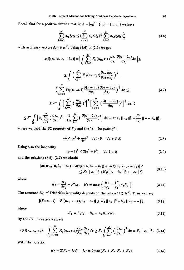
Finite Element Method for Solving Nonlinear Parabolic Equations 65

Recall that for a positive definite matrix A = [aij] (i,j = 1,. . . n) we have

N N N

i , j=l i d = l i~=l (3.6)

with arbitrary vectors ~, r/E R N. Using (3.6) in (3.5) we get

f N .OenO( - ' n ) d x fl i , j=l

f N .0e. 0e. ½ fl i , j=l

N

i , j = l 6qXJ dx <

f " ae,, ~ N O(u--an))2]½ Y J

N i , j=l i , j=l

dx _<

f N Oen)2+ I_L~ O(u-fin) F* _<F* [ e , E ( ~ x / 4~1 ( 07; )2 ]da=F*e l i l e " I I~+~ Iiu-~nil~'

Ill i=1 i=1

where we used the $2 property of Fij and the "e - inequality" :

(3.7)

1 ab 6a 2 +-~b ~ Ve > O,

Using also the inequality (a + b) 2 _< 2(a -~ + b2),

and the relations (3.5), (3.7) we obtain

Va, b E R

Va, b E R

(3.8)

(3.9)

where

la(t)(Un; U, ~n -- Un) -- a(t)(U; U, ~,. -- Un)l + la(t)(u.; en, u -- ~,~)1 ~<

_< K+ II e . I1+ + g a ( l l u - .a,., I1~ + II ~n I1%

g l * Ks = ~ + F*eI ; K3 = max { K1 .1. F

The constant Kn of Friedrichs inequality depends on the region ~ C R N. Then we have

(3.1o)

(3.11)

I(Fo(u, . ,t) - Fo(un, . . . , t ) , ~ , - , , n ) l ~ K4 II ~n II ~ + K s H fin - u I1~,

where K4 = L1¢3; IQ = Lllin/2¢3.

By the $2 properties we have

(3.12)

(3.13)

/ ~ a~nae. / ~ ae . ~

N i , j = l fl i = l

With the notation

dx -- F, [[ en 1112. (3.14)

Ks = 2(F, - Ks); K? = 2max{K3 + Ks, K3 + K4} (3.15)

66 I. F^a, Go

it follows from (3.1) that

d --dr II e. I{ 2 +Ks II en 1112 < Kr[ll u - fin 1121 + II en II 2] + 2 [( . _ ~ , u _ ~ . ) l O e n (3.16)

holds. We choose now the arbitrary numbers q , e2 such that Ks is positive , which is always feasible. Multiplying (3.16) by e -K ' ' and by integrating

d't Led" -K,, II e . II 2) = _K, ,da t II en II 2 - K r e - K ' ' II e . II 2 (3.17)

on the interval (0, r) (0 < r < T is arbitrary) we obtain the inequality

1"

e - K ~ t II e,., II 2 ( , ' ) - II er, II 2 (0) + Ks / e - ~ ' ' II e,., II 2 dt <_

o (3.18) 9"

_ d, I 0 0

We now give an estimation for the last component of the right side. An integration by parts immediatly results

1"

- f~n / dt = B1 - B2, (3.19) u

o

where BI = [eK"(en, u - u.)],=o,

I"

o

Since Kr is positive it is easy to show that

holds. We introduce the notations

It is clear that

< [.. , +__1 ]. - - 4C4 II u - ,~. II 2 ,=o

(3~ = f l x (0, r), 1"

II ~ IIL(,~,)=( f II ~(.,t)II 2 dt ); 0

v E L2(0,T, L2(f~)).

(3.20)

(3.21)

(3.22)

2 2 (3.23) II v llL~<q,)~ll v IIL~<qT) ' By applying the Cauchy-Schwarz inequality and (3.23) we obtain

B2 L~(qT) +4--ff II en ilL,(qT) +KT~s II u - u,, llL~(q~) + 4--~ II e- llL~(q~) • 6 5 11 a t II

(3.24) A summation yields

I"

"Yi-' u - ~ . ) dL < Ks[II e,, II 2 ( r ) + II e,, IlI,(,~.)]+ o (3.25)

O(u t~.) 2

Finite Element Method for Solving Nonlinear Parabolic Equations 67

where Ks = maz{¢4; 1/4¢5 + K7/4¢s},

K9 = maz{Kz¢6; ~5; 1/465}.

We introduce the following norms:

T

II v [l~g×L~(O,~.)= f II ~ 1112 dr, 0

II ~ IIL2xC(O,T) = sup II v(.,0 II. 0_<,_<T

(3.26)

(3.27)

K,2 = max{K7 + 2]~5/(9 , 2K9 + 1} (3.34)

Since for arbitrary fixed r E [0, T]

I[ v I[H0~xL~(0,r)_<[[ V []H]xL~(0,T) (3•35)

holds, inequality (3.33) implies

2 II e. IIL~xc(O,T) +K13 II e. II~×L~(O,T)_<

- [[Hg×L.(O,T) + + II ~ - ~ . IIL2xC(O,T) with the notation

K13 = KI1/K12; I(14 = K12/Klo; KlS = 21£'14 (3.37)

Thus we have proved the following theorem:

where

The Friedrichs inequality and (3.27) imply

2 II ~ II~=<Q,)< g?~ II ~ llH~xn=(o,,), " ~ (0, T)] (3.28)

The relation e -g'T <_ e -K'T < 1, (3.28), (3.25) imply that inequality (3.18) can be written in the form

2 II e . II ~ ( , ' ) [e - K ' T - 2 K ~ ] + II e. [IHo'×L~(o,.) [ K s e - K ' T -- 2 K s K n ] <

• [ a ( u - u") -~"2(QT) (3.29) < _ 2K9 at + 2 K 9 II u - ~ . II 2 ( ~ ) + II e . II 2 (0)

Notice that (2.9) and (2.12) imply

(u(.,0)- u,(.,o),~} ")) = 0; i= 1,2,... ,n. (3.30)

Hence en(O) is orthogonal to H (n), that is for arbitrary un

II e . II 2 (0) <11 u - ~ . II 2 (0). (3.31)

holds• Let us choose the arbitrary positive constants e4, e5 and e6 such that the relations

KI0 = e - K ~ T - - 21Q > 0,

K l l = K 6 e - K ' T - 2KsKn > 0 (3.32)

hold. Then inequality (3.29) changes to

2 K10 l[ en II 2 (r) + Kl l [Ien IlHolxL~(0,r)~

] - IlHo'XL2(0,r) "1- 0t La(QT) + II U -- ,~. [Ig~xc(O,T)

68 I. F,P~OO

Theorem 3.1

Let denote by u(z, t) the solution of problem (2.1) - (2.3); un(z,t) the semidiscrete Galerkin approximation given by the solution of problem (2.11),(2.12) and let fin(z, t) E C(0,T; H (n)) be arbitrary. Then for the error function en(Z,t) = u(z,t) - Un(Z,t) we have the estimation (3.36), where Kls and K15 are independent constants of n.

Remark 3.1

The error estimation remains valid for the S1 conditions too.

Theorem 3.~

The Galerkin sequence is convergent in the L2 × C(0, T) and the H01 × L~(0, T) norms for both sets of conditions $1 and $2.

PROOF. The right side of (3.27) depends on the approximation of u(z, t) in the space C(O,T;H(")). We know that f~ is a regular domain. Therefore the statement of the theorem follows from the completness of the spline functions in space H0X(f~).

The order of the convergence is determined by the order of the approximation. For example, let us consider the region having the form of rectangle in R 2 : ~ = (a, b) x (c, d). Let denote by A the partition of fl by rectangles (zi, Zi+l) x (yj;yj+l). We denote by H(m)(A, f~) the set of those functions w(z, y) which are defined on fl and satisfy the condition

Oi+Jw 0z i 0yJ e C°'°(f2), (0 ~ i, j ~ m - 1) (3.38)

Furthermore we suppose that w(z, y) is pohnominal of degree 2m - 1 on each elemantary rect- angles. Let f be a function such that the conditions

Oi+Jf OziO--'--- ~ 6 C°'°(G), i f i + j < 2m (3.39)

Oi+Jf OxiO------ ~ E L.~(f~), i f i + j --- 2m (3.40)

are valid. Then there exists a function fh E H(m)( A, f~) such that

01+J n ~ ( f - fh) <_ Cfh 2m-(i+j), (3.41)

holds if i + j < 2 m - 1,0 < i , j < m and C! is a constant depending on Ilfll2 . [2]. Using (3.36) we have

e 2 2 [[ ,[[L2xC(O,T) + [e"]H~×L3(O,T) <- Ch2(~'m-1)" (3.42)

We note that error-estimation (3.42) coincides with estimations known for linear problems [7]. When the estimation

sup [[e.[[(t) < Ch r (3.43) O<_t<T

is directly obtained from (3.42) then we get an estimation which is relatively worse than the linear ones by a factor of h½ [7].

1.

REFERENCES

G.A. Baker, V.A. Dougalis, O. Karakasian, On multistep Galerkin d]scretlzations of sernillnear hyperbolic and parabolic equatlons, Nonlin, Anal. 4, 579-597 (1980).

Finite Element Method for Solving Nonlinear Parabolic Equations 69

2. G. Birkhoff, M. Schultz, R. Varga, Piecewise Hermite interpolation in one and two variables, N~m. Math. 11, 232°256 (1968).

3. J. Denel, F. Hess, Nonlinear parabolic boundary value problems with upper and lower solutions, Isr. J. of MaO~. 29, 92-104 (1978).

4. J. Douglas, T. Dupont, Galerkin methods for parabolic equations, S I A M J N~m. Anal. 7, 575-626 (1970). 5. J. Douglas, T. Dupont, M. Wheeler, A quasi-projection analysis of Galerk/n methods for parabolic ang

hyperbolic equations, Math. Comp. 23, 345-362 (1978). 6. I. Fara66, Finite element method to solution of elliptic problems, Alk. Mat Lapok 8,399-425 (1982). 7. I. Farag6, Finite element method to solution of linear parabolic problems, Alk. Mat Lapok 11, 123-155

(1985). 8. I. Farag6, Convergence of semidiscrete Galerkin approximation for parabolic equations with signdeterra/nated

nonlinearity, Nnm. Math. Coll. Soc. Janom Bolyai 50, 371-380 (1987). 9. I. Farag6, A. Ga]Antai, An A-stable three-level method for the Ga]erkin solution of quasilinear parabolic

problems, Nora. aec. Comp~for~ca 9, 67-80 (1988). 10. B. J. Omode[, On the numerlcal stability of the l~yleigh-l~tz method, S I A M J. Num. A n a l 14, 1151-1171

(1977). 11. H.H. Rac~ord, Two level c]Jscrete-tlme Galerkin approximations for second order nonlinear parabolic partial

differential equations, S I A M J. N~m. Anal. 10, 1010-1026 (1973). 12. M. Wheeler, A priori L2-error estimates for Galerkin approximations, S I A M J. N~m. Anal. 10, 1723-1759

(1973).