Finite Element Approximation of Solutions to a Class of NonlinearHyperbolic-Parabolic EquationsDonald A. French�Department of Mathematical Sciences, University of Cincinnati, Cincinnati, OH 45221S�ren JensenyDepartment of Mathematics and Statistics, University of Maryland Baltimore County, Baltimore, MD 21250Thomas I. SeidmanzDepartment of Mathematics and Statistics, University of Maryland Baltimore County, Baltimore, MD 21250January 13, 1999AbstractThe numerical approximation of Antman and Seidman's model [AS] of the longitudinalmotion of a viscoelastic rod is investigated. Their constitutive assumptions ensure that in�nitecompressive stress is needed to produce total compression of the rod. Analyses of the regularityof the solution of the continuous problem, the convergence of a semi-discrete �nite elementmethod, and the properties of a space-time �nite element scheme are furnished. Results of asample computation are also provided.1. Introduction:Consider the following model for the longitudinal motion of a visco-elastic rod:wtt = [n (ws; wst)]s + f (1)where w = w(s; t) is the position at time t of the point with reference position s so ws is thestrain and wst is the strain rate; n is then the contact force and f is the body force. A natural set�Work was carried out while French was a visitor at the University of Maryland Baltimore County during 1995-6,at his current position at the University of Cincinnati during 1996-7, and while he was on sabbatical at the Institutefor Mathematics and its Applications and the University of Minnesota Mathematics Department during 1997-8. Hisresearch was supported in part by the Taft Foundation at the University of Cincinnati through their Grants-in-Aidprogram.yResearch partially supported by the ONR Contract No. N00014-90-J-1238.zResearch partially supported by grants AFOSR-82-0271 and AFOSR-87-01901

of boundary conditions for this problem consists of the speci�cation of the contact forces at theendpoints; n (ws; wst)���s=0 = n0(t) n (ws; wst)���s=1 = n1(t) (2)where n0 and n1 are given. The initial conditions we use arew(�; 0) = w0 and wt(�; 0) = v0 (3)where w0 and v0 are given. For simplicity we have restricted our attention to a homogeneous rodwith constant mass density equal to 1 and the constitutive function n independent of s.This model was considered in [AS] under assumptions on the constitutive function n permittingfully nonlinear dependence on the strain rate while ensuring well-posedness and that one neverdevelops `in�nite compression': that is, ws is pointwise bounded away from 0.Observe that in terms of the function w the equation (1) is essentially hyperbolic. However, ifwe reformulate it in terms of u := ws and v := wt to obtainut = vs and vt = [n(u; vs)]s + f (4)the second equation is parabolic in v if we think of u as being known.It will also be convenient to split the contact force:n(y; z) = �0(y) + �(y; z) (5)so � is the elastic potential and �(y; z) is the viscous part. Here we will impose the following setof constitutive hypotheses: (much as in `Note Added in Proof' of [AS])(H0) (Properties of �) The elastic potential �(y) is minimized at y = 1 (equilibrium) so that� : (0;1)! [0;1) and one has �0(y)!1 as y ! 0;1.(H1) (uniform ellipticity) There is some m > 0 such thatnz(y; z) � m for z 2 IR; y > 0; (6)and thus �(y; z)z � mz2.(H2)(Control of compression) There are A;M > 0 and a (nonincreasing) function : (0; y�) !(0;1) with (y)!1 as y ! 0+ such that, for some y� > 0,n(y; z) � A+M (y)� 0(y)z (7)for z 2 IR, 0 < y < y�.(H3) (Growth of n) For each � > 0 there exists � = �(�) such thatjny(y; z)j � �nz(y; z) and jny(y; z)j � �qnz(y; z)s j�(y; z)jjzj (8)2

for z 2 IR, y > �.In this report we provide a survey of our initial investigations into numerical methods for thishighly nonlinear problem. In section 2 an analysis of the solution to the continuous problem, (1){(3) is given. We show several energy estimates and demonstrate the lower bound estimate for thestrain ws. In section 3 an example is given by explicit formula for a contact force function n whichsatis�es hypotheses (H0){(H3) (as well as (H4) and (H5) which will be introduced later). In sections4 and 5 a semi-discrete �nite element is introduced (discrete in the space variable s and continuousin time t), energy estimates and the strain lower bound property are derived for the approximationfunction wh and an error estimate is provided. In section 6 an implicit fully discrete numericalmethod is used in a sample computation. This scheme uses the �nite elements from section 4 anda simple centered di�erence scheme for the time discretization. Finally, in section 7 another fullydiscrete method is described using �nite elements in both space and time. The special feature ofthis third method is that it preserves the lower bound property for the numerical strain, whks .We will use C generically to denote a positive constant for which we have an upper boundeither absolute or depending only on the various parameters in (H0)-(H3), on the data norms, onT , and on previous occurrences of C, but not dependent on the particular data or the particularsolutions involved. In particular, C will never be dependent on the mesh parameter h which wewill introduce in section 4.We note that this paper is a continuation of the work by the �rst two authors in [FJ]. In thatpaper energy properties of a space-time �nite element method which resembled those for a certainviscoelastic rod problem were derived. In that model, however, the possibility of total compressionwas not considered as it is in this work.Acknowledgement: The second author, S�ren Jensen, passed away during the course of this work.He is greatly missed by us all. We acknowledge his signi�cant contributions and participation inall aspects of this project except the �nal writing.2. The Continuous Problem:In this section we will provide a simpli�ed version of the principal results of [AS], restricted to thecontext described above. The principal e�ort is to obtain a priori estimates for the solution, inparticular obtaining pointwise estimates for the arguments ws and wst. We �x T > 0 arbitrarilyand assume the following, in addition to the constitutive hypotheses (H0){(H3) above:(A0) The data for the problem, functions f; n0; n1; w0 and v0 are as smooth as needed. Alsow0;s � y� > 0 with y� as in (H2).First energy estimate:The total energy for the rod (kinetic plus elastic potential) isE(t) = 12kwtk2 + Z 10 �(ws) ds3

where jj � jj is the L2(0; 1) norm (k � k1 will denote the L1(0; 1) norm) and the work done bydissipated stress is W (t) := Z t0 �Z 10 �(ws; wst)wst ds� dt:Using the equation (1) and an integration by parts givesddt [E +W ] = Z 10 fwt ds+ n1wt���s=1 � n0wt���s=0� 12kfk2 + 12kwtk2 + 12 jn1j2 + 12 jn0j2 + � Z 10 �(ws; wst)wst ds+C�kwtk2where we used the fact that for any � > 0 there is a constant C� such thatjg(s)j � �kgsk+ C�kgkfor any s 2 (0; 1) and any g 2 H1. In view of (H1),kwstk � C �kwtk2 + 2 Z 10 �(ws; wst)wst ds�1=2 :Taking � = 12 to subtract that term from dW=dt, integrating over (0; t), and applying the Gronwallinequality, we obtain the estimates:kwt(�; t)k; �(t) := Z 10 �(ws) ds; W (t) � C: (9)Lower bound for ws:Suppose one has ws(�s; �t) < y� for some (�s; �t) 2 Q := (0; 1)� [0; T ]. Then there is a � > 0 such thatws(�s; t) < ws(�s; �) = y� for � < t � �t. Integrating (H2) with y = ws; z = wst over (�; t) then gives (ws(�s; t))� (y�) = Z t� 0(ws)wst dt̂ � Z t� [A+M (ws)� n(ws; wst)] dt̂:Since integrating (4) over (0; �s) gives n(ws; wst)����s;t = n0 + R �s0 [wtt � f ] ds, we then have (ws(�s; t)) � � (y�) +A(t� �)� Z t� n0dt̂+ �Z �s0 wt ds� j�t� � Z t� Z �s0 fdsdt̂�+M Z t� �ws����s� dt̂:The bracketed terms on the right can all be estimated (using (9) for the R wtt ds terms) so theGronwall inequality gives an upper bound for (ws(�s; �t)), which we note is uniform for any (�s; �t) 24

(Q) for which ws(�s; �t) < y�. Since (y) ! 1 as y ! 0, this implies a positive pointwise lowerbound: ws(s; t) � �y� > 0: (10)Second energy estimate:The equation (1), formally di�erentiated with respect to t, giveswttt = [nywst + nzwstt]s + ft: (11)Using 2wtt as test function in the weak form of this giveskwttk2 + 2 Z t0 Z 10 nzw 2stt ds dt̂ = kwtt(�; 0)k2 + 2�Z t0 n1wtt���s=1 dt̂+ Z t0 n0wtt���s=0 dt̂�+ Z t0 Z 10 (ftwtt � nywstwstt) ds dt� kwtt(�; 0)k2 + Z t0 akwsttk dt̂+ 2� Z t0 Z 10 jpnzwstj p�wstt ds dt̂where a 2 L2(0; T ) depends on the data f; n0; n1. This givesZ t0 akwsttk � kak2 + � Z t0 Z 10 nzw 2stt dt̂+ C� Z t0 kwttk dt̂;and we have estimatedjnywstwsttj � � jpnzwsttjqj�wstj � �nzw 2stt + C�j�wstjusing (8) with y = ws; z = wst. It follows thatkwttk2 + Z t0 Z 10 nzw 2stt ds dt̂ � �kwtt(�; 0)k2 + kak2 + C� Z t0 Z 10 �wst ds dt̂�+ C� Z t0 kwttk2:Noting that the double integral term on the right side of the equation is just W (t), for which wealready have the bound (9), we apply the Gronwall inequality and obtain the estimates:kwttk ; Z t0 kwsttk2 dt̂ � C: (12)Third energy estimate:If we rewrite (4) as wtt = [nywss + nzwsst] + f we can solve for wsstwsst = wtt � fnz � �nynz�wss:5

Taking norms and using (H1), (H3), giveskwsstk � C �kwttk+ 1mkfk�+ �kwssk (13)and, integrating, kwssk � kwss(�; 0)k + 1m Z t0 [kwttk+ kfk] dt̂+ � Z t0 kwssk dt̂:Applying the Gronwall inequality to this bounds kwss(�; t)k and using that in (13) gives:kwssk ; kwsstk � C: (14)Pointwise bounds for ws and wst:To obtain pointwise bounds for ws and wst we need (14) and knowledge that ws and wst are boundedat some point s on [0; 1] to apply the Poincar�e inequality: in particular at s = 0 and s = 1.Observe from (H1) that n is invertible in its second argument. Thus there is a function g =g(u; n) such that g(y; n(y; z)) = z. Further, from (H1) and (H3) we have,gu = �nynz so jguj � �and gn = 1nz so jgnj � 1m:Since n = n0 at s = 0 and n = n1 at s = 1 we have that n is a C1 function at s = 0 or s = 1. Thenew de�nition of the function g allows us to specify ws by an ordinary di�erential equation (ODE)which is ddtws = g(ws; n)where as noted above n is speci�ed as a function of t at s = 0 and s = 1. Combining the results onthe bounds for g and the de�ning ODE we conclude that both ws and wst are bounded at s = 0and s = 1 as asserted. These facts combined with (14) and (10) allow us to conclude that0 < �y� � ws � �y� and jwstj � �z� (15)where both results are on the space time domain Q. >From now on, keeping (15) in mind, we willassume pointwise uniform bounds on n, ny, nz, nzy and nzz.The above results and arguments can be easily used to prove there exists a unique solution tothe problem. We refer the reader to [AS] for more on these technical aspects. We are now in aposition to state our main theorem on the continuous problem.6

Theorem 1: (Global existence and uniqueness): Suppose the data for the problem satisfy as-sumption (A0) and the constitutive function n satis�es the hypotheses (H0){(H3). Then the ini-tial/boundary value problem de�ned by (1){(3) has a unique solution, w, on the domain Q for anyT > 0 and w satis�es the uniform norm inequalities (9), (12), (14), and (15).3. Example Constitutive Law:To show the consistency of the set of hypotheses (H0){(H3) (as well as (H4) and (H5) which willbe introduced later) we provide an explicit formula for n(y; z) which satis�es them. It is this con-stitutive law which will be used later for the computational example. The functions n and nz willbe continuous and the derivatives ny, nyz and nzz will be de�ned on the domain of de�nition whichis y > 0 and �1 < z <1.We take �(y) = 2y + y2 (16)to satisfy the hypothesis (H0). The de�nition of � is much more complicated;�(y; z) = 8>>>>><>>>>>: z � 12z2 if z � 0 and y � 1z � 12z2 � 12(1� y�2)2 if z � 0 and (1� z)�1=2 � y < 1zy�2 if z � 0 and 0 < y < (1� z)�1=2z if z > 0 and y � 1z + (y�2 � 1)�(z) if z > 0 and 0 < y < 1 (17)where �(z) = ( z + z2 � z3 if 0 � z � 11 if z > 1:Note that �(y; z)=z � 1; this will be used later to verify the second part of (H3). To check hypothesis(H1) we di�erentiate � with respect to z. This gives�z(y; z) = 8>>><>>>: 1� z if z � 0 and y � (1� z)�1=2y�2 if z � 0 and 0 < y < (1� z)�1=21 if z > 0 and y � 11 + (y�2 � 1)�0(z) if z > 0 and 0 < y < 1where �0(z) = ( 1 + 2z � 3z2 if 0 � z � 10 if z > 1:It follows that (H1) holds with m = 1; a crucial step is to note that �0(z) � 0 for 0 � z � 1. Alsonote here that �yz and �zz are de�ned and piecewise continuous.7

To verify (H2) we take (y) = y�1 and y� = 1. It follows that 0(y) = �y�2 and thus the upperbound on n is A+My�1 + zy�2in the region where 0 < y � 1. Perhaps the most di�cult veri�cation is in the region where(1� z)�1=2 � y � 1 and z � 0. Here, we haven(y; z) = 2(�y�2 + y) + (z � 12z2 � 12(1� y�2)2) � 1 + z � 1 + zy�2which gives (H2) if we take A � 1 and M � 2.To verify (H3) we will need to evaluate the y-derivative.ny(y; z) = (�4y�3 + 2) + �y(y; z)with �y(y; z) = 8>>>>><>>>>>: 0 if z � 0 and y � 12(1� y�2)y�3 if z � 0 and (1� z)�1=2 � y < 1�2zy�3 if z � 0 and 0 < y < (1� z)�1=20 if z > 0 and y � 1�2y�3�(z) if z > 0 and 0 < y < 1:Thus, in the region where z � 0 and y � � > 0 we havejny(y; z)j � 6y�3 + 2 � (6��3 + 2)qj�z(y; z)js�(y; z)z = (6��3 + 2)qjnz(y; z)js�(y; z)z :The other inequalities follow similarly in the other regions.4. The Semi-Discrete Finite Element Method:Let V h be the space of continuous piecewise linear functions de�ned on the partition with nodessp = ph and parameter h = P�1 where P is a positive integer; we embed this in L2(0; 1) with theinduced inner product. Let Ip = (sp�1; sp) and wh;ps (t) = whs (�; t)���Ip which is a constant. A spatiallydiscrete �nite element method can then be constructed as follows: Find wh(�; t) 2 V h for 0 < t < Tsuch that (whtt; �) + (n(whs ; whst); �s) = (f; �) + n1�(1)� n0�(0) (18)for all � 2 V h where wh(�; 0) �= w0 and wht (�; 0) �= v0. We observe that this problem has a uniquesolution, at least for short time. Since V h is a �nite dimensional space, a basis for it can be foundand from this a system of ordinary di�erential equations can be derived. As long as n is well de�nedthere exists at least a short time solution.For the error estimate we will make the following regularity assumption:8

(A1) Function wstt 2 L1(Q) and for all t 2 [0; T ], wsstt 2 L2(0; 1).We also will need an extra smoothness assumption on the constitutive law, valid for our example.(H4) Functions nyz and nzz are piecewise continuous in y; z.Note that our explicit constitutive formula (16){(17) satis�es (H4). We also note that, withoutproof, an argument similar to those of section 2 (di�erentiate (11) yet again with respect to t,expand, and estimate the term on the right to get a di�erential inequality for kwtttk2) gives (A1)for some time interval.Energy bounds for wh:One can apply the �rst energy argument of section 2 to the semi-discrete problem and show that,similarly, Z t0 kwhstk2d�; kwtk; Z 10 �(whs )ds � C: (19)One can also apply the lower bound argument to obtainwhs (s; t) � �ySD� > 0on Q where �ySD� is a constant that is independent of h. The notation SD stands for semi-discrete.The second energy argument can be applied by di�erentiating the variational equation de�ning whwith respect to t. This gives(whttt; �) + (nywhst + nzwhstt; �s) = (ft; �) + n01�(1)� n00�(0):By taking � = 2whtt, integrating over time, one can show the same estimates for wh as was done insection 2 for w: kwhttk; Z T0 kwhttskd� � C: (20)Bounds at the boundary:De�ne �p(s) = 8><>: 0 if 0 < s < sp�1s� sp�1 if sp�1 < s < sp1 if sp < s < 1 : (21)Then, taking �P as the test function in (18) gives the equationhn(wh;Ps ; wh;Pst ) = (f; �P ) + h(n1(t)� n0(t))� (whtt; �P ):Multiplying by wh;Pst and noting that k�pkL1(0;1) � h we havemjwh;Pst j � (kfkL1(0;1) + jn1(t)j+ jn0(t)j+ kwhttk)9

and, since the quantities on the right are bounded, we conclude thatjwh;Pst j � CSince wh;Ps (t) = wh;Ps (0) + Z t0 wh;Pst (�)d�we have that jwh;Ps j � C:A similar bound can be found for wh;0s (t).Interior pointwise upper bound for whs :Using � = �p in (18) we obtain hn(wh;ps ; wh;pst ) = (f � whtt; �p)for each 0 < p < P . Subtracting the (p� 1) equation from the p equation, we obtainh(n(wh;ps ; wh;pst )� n(wh;p�1s ; wh;p�1st )) = (f � whtt; �p � �p�1)where, using the Taylor theorem along the segment joining (wh;p�1s ; wh;p�1st ) to (wh;ps ; wh;pst ),wh;pst � wh;p�1st = (f � whtt; �p � �p�1)hnz( ; �) � ny( ; �)nz( ; �) (wh;ps � wh;p�1s )for some pair ( ; �) on the segment. De�ne @puh = uh;p�uh;p�1, where uh is any piecewise constantfunction de�ned on the mesh, as whs and whst. ThenPXp=1 j@pwhstj � 1m PXp=1 kf � wttkL1(Ip) + � PXp=1 j@pwhs j (22)where � is de�ned in (H3). Since kf � whttkL1(0;1) is bounded independently of h, it follows from aGronwall argument that PXp=1 j@pwhs j � Cand using this in (22) gives PXp=1 j@pwhstj � C:10

To obtain an upper bound on wh;ps we havewh;ps = @pwhs + wh;p�1s= @pwhs + @p�1whs + : : : @1whs + wh;0sso jwh;ps j � PXp=1 j@pwhs j+ jwh;0s j � C:In the same way we as for (15) we also �ndjwh;pst j � C:We are now in a position to state our �rst theorem on the properties of the semi-discrete method.Theorem 2 (Stability of the semi-discrete scheme): Assume the hypotheses (H0){(H3) hold onn and assumption (A0) is valid for the data. Then the numerical method de�ned by (18) has aunique solution which satis�es the inequalities (19), (20), and the pointwise bounds0 < �ySD� � whs � �ySD;� and jwhstj � �zSD;�: (23)As with the continuous solution we can assume pointwise bounds for n, ny, nz, nzy, and nzz |uniform on the relevant domain.A rede�nition of n(�) o� the estimated domain occurs in the existence proof but is not neededfor implementation. It is important to realize that the implementation of this scheme does notinvolve any computation of the bounds (23) which we have noted to justify it.5. Error Estimate for the Semi-Discrete Method:In this section we will use the uniform bounds obtained in the previous section and a nonlinearRitz projection to obtain an error estimate. We �rst de�ne and analyze our projection, which isused in the error estimation but not in the actual computations.Ritz Projection:Consider �nding �h(�; t) 2 V h so for each t(n(ws; �hs ); �s) = (n(ws; wst); �s) (24)for all � 2 V h where Z 10 �hds = Z 10 wtds: (25)We will now show that there exists a unique �h that satis�es (24) and (25) and view this constructionas a nonlinear map, called the Ritz projection: wt ! �h.11

Existence of the Ritz projection:We will use the following version of Brouwer's �xed-point theorem to show there exists a solutionto (24) (see [GR], Corollary 1.1, p. 279):Let H be a �nite-dimensional Hilbert space with inner product h�; �i and corresponding norm j � j.Let : H ! H be a continuous mapping with the following property. There exists a � > 0 suchthat h(g); gi � 0 8g 2 H with jgj = �: (26)Then, there exists a g� 2 H with jg�j � � such that (g�) = 0.To apply this to our situation, we �rst rewrite (24) as follows: Instead of �h we seek ~�h 2 V h0 =f� 2 V h : R 10 �ds = 0g such that (n(ws; ~�hs ); �s) = (n(ws; wst); �s)where ~�h = �h �Mv with Mv = Z 10 wtds = Z 10 �hds:Note that this problem is equivalent to (24). We set the Hilbert space H = V h0 with the innerproduct h�; �i = Z 10 �s�sdsand take g = ~�h. Then h(g); �i := (n(ws; gs); �s)� (n(ws; wst); �s);but h(g); gi = (n(ws; gs); gs)� (n(ws; wst); gs)� mkgsk2 � kn(ws; wst)kkgsk= m��2 � �m��where � = kn(ws; wst)k and � = kgsk. For � � �=m the inequality (26) holds, implying thereexists a solution to the projection problem (24).Uniqueness of the Ritz projection:Suppose (24) might have two solutions �h and ��h. >From the de�ning equation (24) and Taylor'stheorem we have (nz(ws; �)(�h � ��h)s; �s) = 012

for all � 2 V h where � lies between �h and ��h. Choosing � = �h � ��h and using hypothesis (H1)we have mk(�h � ��h)sk2 � 0and, since also Z 10 (�h � ��h)ds = 0we must have �h = ��h.Error estimate for the Ritz projection:Let b(z) = n(ws; z). We will need the following approximation results. We assume there is aninterpolation operator � : H1(0; 1)! V h such that, for any z 2 H1(0; 1) � L1(0; 1),k(I � �)zk � Chkzsk and k�zkL1(0;1) � kzkL1(0;1): (27)We will also use the following standard inverse inequality: for any � 2 V hk�kL1(Ip) � Ch�1=2k�kL2(Ip) (28)where Ip is an interval in the �nite element mesh which has length h (see [C]). Let �b be a C1function with �b(z) = b(z) for jzj � kwstkL1(0;1) + � where � > 0 and such thatk�b0kL1(0;1) � R and �b0 � m:We will analyze the problem: �nd ��h 2 V h such that(�b(��hs ); �s) = (�b(wst); �s) (29)for all � 2 V h and will show that this givesk��hs � wstk � Chkwsstk: (30)>From this we will have thatk��hs k1 � k��hs � �wstk1 + k�wstk1� Ch�1=2k��hs � �wstk+ kwstk1� Ch1=2kwsstk+ kwstk1Choosing h small enough so Ch1=2kwsstk � �13

implies that �b = b for the range of ��hs considered so, since we have uniqueness for (24), it nowfollows that ��h = �h and, setting � = �h � wt,k�sk � Chkwsstk: (31)We now show (30). Note thatZ 10 �b0(wst + � ��s)��s d� = �b(��h)� �b(wst)where �� = ��h � wt. If we then let �B = Z 10 �b0(wst + � ��s) d�;then (29) becomes ( �B��s; �s) = 0and m � �B �M . Then ( �B ��s; ��s) = ( �B��s; (� � I)wst)so mk��sk �Mk(I � �)wstk � Chkwsstkproving (30).Finally, we need an estimate on the t derivative of the error. Di�erentiating the de�ning equation(24) gives(nz(ws; �hs )�hst; �s) + (ny(ws; �hs )wst; �s) = (nz(ws; wst)wstt; �s) + (ny(ws; wst)wst; �s)or(nz(ws; �hs )�st; �s) = �((nz(ws; �hs )� nz(ws; wst))wstt; �s)� ((ny(ws; �hs )� ny(ws; wst))wst; �s):Then, applying the Taylor theorem,(nz(ws; �hs )�st; �s) = (D�s; �s)where D := �(nzz(ws; )wstt + nyz(ws; �)wst):By our assumptions we have that D is bounded in L1 and that and � each lie between �hs andwst. Then (nz�st; �st) = (nz�st; �hst)� (nz�st; wstt)= (D�s; �hst)� (nz�st; wstt) + [�(D�s; �wstt) + nz�st; �wstt)]= (D�s; �st) + (D�s; (I � �)wstt) + (nz�st; (I � �)wstt)14

or mk�stk2 � C(hk�stk+ h2)kwssttkwhich implies k�stk � Chkwssttk: (32)We are now in a position to state the key error estimate for the projection.Lemma: Let �h be the Ritz projection of wt satisfying (24) and (25). Assume the conditions(H0){(H4) hold for n, the data are smooth, (A0), and the solution w is su�ciently regular, (A1).Then the error � = �h � wt satis�es an estimate:k�sk � Chkwsstk and k�stk � Chkwssttk: (33)Error estimate for the semi-discrete problem:We start with a standard splitting for time dependent problems,et = wt � wht = (wt � �h) + (�h � wht ) = �+ �h;and then obtain (�ht ; �) + (n(ws; �hs )� n(whs ; whst); �s) = �(�t; �):Choosing � = �h in (18) we obtain12 ddtk�hk2 + (nz(ws; �)�hs ; �hs ) = �(�t; �h)� (ny( ;whst)es; �hs )= �(�t; �h)� (ny( ;whst) Z t0 (�s + �hs )d�; �hs )where is between ws and whs and � is between wst and whst. Thenddtk�hk2 + k�hs k2 � C(k�tk2 + Z t0 (k�sk2 + k�hs k2)d�:Apply the Gronwall inequality | assuming, for simplicity, that wht (�; 0) = �h(�; t). This givesk�hk2 + Z t0 k�hs k2d� � Ch2which, together with the estimates on �, gives the error estimate described in the theorem below.Theorem 3 (Semi-discrete error estimate): Suppose wh is the solution of (18) and w is the solutionof (1){(3). Assume the conditions (H0){(H4) hold for n; the data are smooth, (A0); the solutionw is su�ciently smooth as in (A1), and wh(�; 0) is the nonlinear Ritz projection of wt(�; 0). Thenkwst � whstkL2(Q) � Ch:15

6. Discretization in Time of the Finite Element Method:In this section we describe a simple fully discrete numerical method. We use the piecewise linear�nite elements described previously for the spatial variable and introduce a centered �nite di�erenceprocedure for the time discretization. Because of the parabolic nature of this problem with respectto wt we have chosen to make the scheme implicit. Partition [0; T ] into Q intervals of lengthk = T=Q with nodes tq = qk. Let Jq = (tq�1; tq) and J = [0; T ]. We linearize the function n withrespect to the z variable using Taylor's theorem about z0 ,n(�; z) = n(�; z0) + nz(�; z0)(z � z0):Taking z = wh;q+1s � wh;q�1s2k and z0 = wh;qs � wh;q�1skleads to the �nite element/�nite di�erence method:(wh;q+1s � 2wh;qs + wh;q�1s ; �) + k2 "((n(wh;qs ; wh;qs � wh;q�1sk ); �s)+ (nz(wh;qs ; wh;qs � wh;q�1sk )wh;q+1s � 2wh;qs + wh;q�1s2k ; �s)#= k2 ((f; �) + n1�(1)� n0�(0)) :Specifying basis functions f�0; : : : ; �P g, we then obtain a system of equations of the form(M + kKq)W q+1 = F nwhere M is the mass matrix, Kq is a sti�ness matrix, W q has the coe�cients of the basis functionsin wh;q, and F q has all the other terms that involve quantities on the q and q� 1 time levels. Notethat Mij = (�i; �j); Kqij = (nz(wh;qs ; wh;qs � wh;q�1sk )�j;s; �i;s) and wh;q(s) = PXj=0W qj �j(s):As starting data for this multistep method we takewh;0(sp) �= w(sp; 0) and wh;1(sp) �= w(sp; 0) + kwt(sp; 0)for p = 0; 1; : : : ; P . The trapezoid rule is used for the evaluation of all the spatial integrals thatarise. 16

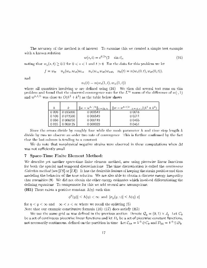
The accuracy of the method is of interest. To examine this we created a simple test examplewith a known solution w(s; t) = e0:2s(2� sin t); (34)noting that ws(s; t) � 0:2 for 0 < s < 1 and t > 0. For the data for this problem we letf = wtt � ny(ws; wst)wss � nz(ws; wst)wsst; n0(t) = n(ws(0; t); wst(0; t));and n1(t) = n(ws(1; t); wst(1; t))where all quantities involving w are de�ned using (34). We then did several test runs on thisproblem and found that the observed convergence rate for the L1 norm of the di�erence of w(�; 1)and wh;1=k was close to O(h2 + k2) as the table below shows.h k kw � wh;1=kkL1(0;1) kw � wh;1=kkL1(0;1)=(h2 + k2)0.200 0.025000 0.002512 0.06180.100 0.012500 0.000519 0.05110.050 0.006250 0.000118 0.04650.025 0.003125 0.000029 0.0451Since the errors divide by roughly four while the mesh parameter h and time step length kdivide by two we observe an order two rate of convergence. This is furthur con�rmed by the factthat the last column is tending to a constant.We do note that nonphysical negative strains were observed in these computations when �twas not su�ciently small.7. Space-Time Finite Element Method:We describe yet another space-time �nite element method, now using piecewise linear functionsfor both the spatial and temporal discretizations. The time discretization is called the continuousGalerkin method (see [FS] or [FJ]). It has the desirable feature of keeping the strain positive and thusmodeling the behavior of the true solution. We are also able to obtain a discrete energy inequalitythat resembles (9). We did not obtain the other energy estimates which involved di�erentiating thede�ning equations. To compensate for this we add several new assumptions:(H5) There exists a positive constant �(�) such thatj�00(y)j � �(�) <1 and j�y(y; z)j � �(�)jzjfor � < y <1 and �1 < z <1 where we recall the splitting (5).Note that our example constitutive formula (16){(17) does satisfy (H5).We use the same grid as was de�ned in the previous section. Denote Qq = (0; 1) � Jq. Let Ckbe a set of continuous piecewise linear functions and let Dk be a set of piecewise constant functions,not necessarily continuous, de�ned on the partition in time. Let Chk = V hCk and Dhk = V hDk.17

We are now in a position to de�ne our numerical scheme. Find (whk; vhk) 2 Chk�Chk such that(whkt � vhk; �)Q = 0 8� 2 Dhk (35)(vhkt ; �)Q + (n(whks ; whkst ); �s)Q = (n1; �(1; �))J + (n0; �(0; �))J + (f; �)Q 8� 2 Dhk (36)where whk(�; 0) �= w0 and vhk(�; 0) �= v0 are given. For any domain A we use the inner product(�; �)A = ZA ��dA giving k�kA = �ZA �2dA�1=2 :The problem can also be de�ned in a slab-by-slab manner by the equations(whkt � vhk; �)Qq = 0 8� 2 V h P0(Jq) (37)and(vhkt ; �)Qq +(n(whks ; whkst ); �s)Qq = (n1; �(1; �))Jq +(n0; �(0; �))Jq +(f; �)Qq 8� 2 V hP0(Jq): (38)The discretization in time can be rewritten as a �nite di�erence scheme. Let whk;q = whk(�; t) andde�ne vhk;q similarly. Assuming that whk;q�1 and whk;q are known, the approximation is found onthe next step by solving the following nonlinear system for whk;q+1(whk;q+1 � 2whk;q + whk;q�1; �) + k22 N(whk;q+1s ; @twhk;q+1=2s )�N(whk;qs ; @twhk;q+1=2s )whk;q+1s � whk;qs+ N(whk;qs ; @twhk;q�1=2s )�N(whk;q�1s ; @twhk;q�1=2s )whk;qs � whk;q�1s ; �s!= k2 ��n1�(1) + �n0�(0) + ( �f; �)�for all � 2 Vh where �ni = 1k ZJq ni dt for i = 0; 1; �f = 1k ZJq f dt;@twhk;q+1=2s = 1k �whk;q+1s � whk;qs � ; @twhk;q�1=2s = 1k �whk;qs � whk;q�1s � ;and N(y; z) = Z y0 n(~y; z)d~y:Note that we are assuming that the spatial integrals are done exactly. In practice one would useeither a �xed point or Newton iteration to solve the nonlinear system on each time step.Discrete energy bounds: 18

We will develop a discrete version of the �rst energy inequality in this context. We �rst note somesimple inequalities that will be useful. LetAu = Z 10 u dsbe an average of u so ju(s)�Auj � kusk (39)and kAukJq � kukQq : (40)De�ning the discrete kinetic energy Khkq = 12 Z 10 (vhk;q)2 dswe have, after taking � = whkt in (37), kwhkt kQq � kvhkkQq (41)and, since vhk is linear in t, kvhkkQq � 2kmaxfKhkq�1;Khkq g: (42)Let � = vhkt in (37) and � = whkt in (38). ThenEhkq + ZJq Z 10 �(whks ; whkst )whkst dsdt = Ehkq�1 + (n1; whkt (1; �))Jq � (n0; whkt (0; �))Jq + (f;whkt )Qqwhere Ehkq = Khkq + Z 10 �(whk;qs ) ds:We now estimate the boundary terms,(n1; whkt (1; �))Jq = (n1; (I �A)whkt (1; �))Jq + (n1; Awhkt (1; �))Jq� C�kn1k2Jq + �4kwhkst k2Qq + 2kmaxfKhkq�1;Khkq gwhere we used (39), (40), (41), and (42) as well as Young's inequalityjabj � �a2 + C�b2for � > 0. A similar inequality can be found for the n0-term. Using the boundary term estimateand applying Young's inequality to the f -term gives,Ehkq +ZJq Z 10 �(whks ; whkst )whkst dsdt � Ehkq�1+�kwhkst k2Qq+C�(kn0k2Jq+kn1k2Jq+kfk2Qq)+4kmaxfKhkq�1;Khkq g:19

Using hypothesis (H1), choosing � = m=2, and noting thatmaxfKhkq�1;Khkq g � Ehkq�1 +EhkqgivesEhkq + 12 Z tq0 Z 10 �(whks ; whkst )whkst dsdt � 1 + 4k1� 4k (Ehkq�1 + 12 Z tq�10 Z 10 �(whks ; whkst )whkst dsdt)+C(kn0k2Jq + kn1k2Jq + kfk2Qq)if k is su�ciently small. Iterating this estimation gives the discrete energy inequalityEhkq + 12 Z tq0 Z 10 �(whks ; whkst )whkst dsdt � Ctq (Ehk0 + Z tq0 n20dt+ Z tq0 n21dt+ Z tq0 kfk2dt: (43)Total compression for the numerical MethodIn this section we show that the approximation will imitate the true solution in that it never su�erstotal compression. A mild restriction will be placed on the time step and spatial re�nement toachieve this. Just to simplify the presentation of the argument, we set n1 = 0 and f = 0.>From the energy inequality (43) there exists a constant C such thatZJq ZIp(whkst )2 ds dt � C:Since whkst is a constant on Jq � Ip this becomesjwhkst j���Ip�Jq � Cpkh: (44)We will now show that whks cannot jump from above y� to below y�=2 in one time step providedskh � y�4C : (45)>From Taylor and (44) we havewhk;qs = whk;q�1s + kwhkst ���Ip�Jq � y� � Cskh � y�2Suppose y�=4 � whks (�; tq) < y� on Ip (Using the preceeding argument we can show that the straincannot jump from above y�=2 to below y�=4 on one step). If it increases above y� then total20

compression did not occur. If it stays below y� then we must address the possibility of whks ! 0.Recall that the function �p 2 V h P0(Jq) from (21). Substituting �p into (38) for �, we have(vhkt ; �p)Qq+1 = ZJq+1 ZIp n(whks ; whkst ) ds dtand, using hypothesis (H2), we now have(vhkt ; �p)Qq+1 � Akh+M ZJq+1 ZIp (whks ) ds dt� ZJq+1 ZIp 0(whks )whkst ds dtSimplifying, we have on Ip that (whk;q+1s ) � (whk;qs ) +M ZJq+1 (whks )dt+ 1h �Z 10 vhk;q+1�p ds� Z 10 vhk;q�p ds�+Ak:Since ZJq+1 (whks )dt � k( (whk;q+1s ) + (whk;q+1s ))we have on Ip (for 1�Mk � 1=2) (whk;q+1s ) � 1 +Mk1�Mk (whk;qs ) + 2h(Z 10 vhk;q+1�p ds� Z 10 vhk;q�p ds) + 2Ak:Iterating this inequality gives for any integer r > q and since tr � tq < T that (whk;rs ) � CT ( (whk;qs ) + 2h(Z 10 vhk;r�pds� Z 10 vhk;q�pds) + 2AT� CT ( (y�4 ) + 2Khkr +Khkq ) + 2AT ):Since the right side of the equation is bounded there must be a constant �yFD� such thatwhks � �yFD� > 0: (46)Existence and uniqueness for the space time method:In this section we use the strategies given in section 3 to show that the numerical scheme (37){(38)has a unique solution under the constraint that k � �h for some su�ciently small constant �.For existence we use the version of the Brouwer �xed-point theorem which we employed earlier.Let H = V h P0(In), with inner product (�; �)Qq , and norm k � kQq with g = whkt . Then sincewhk(�; t) = whk;q�1 + Z ttq�1 g(�; s)ds21

we can reconstruct whk from g. De�ne((g); �)Qq = (vhkt ; �)Qq + (n(whks ; gs); �s)Qq � (n1; �(1; �))Jq � (n0; �(0; �))Jq � (f; �)Qqwhere vhk is de�ned from g and vhk;q�1 through (37). Taking � = g and arguing as we did in theenergy inequality (to prove (43) ), we obtain((g); g)Qq � (1� Ck)Ehkq � (1 + Ck)Ehkq�1 � C(kn1k2Jq + kn0k2Jq + kfk2Qq) +Ckgsk2Qq :Using the Poincar�e inequality, there is a positive constant C such thatkgsk � C �kgk � ����Z 10 gds�����so kgskQq � C(kgkQq � Ck(Ehkq +Ehkq�1))Thus for su�ciently small k we have((g); g) � CkgkQq � C(Ehkq�1 + kn1kJq + kn0kJq + kfkQq)We conclude that one can force ((g); g)Qq > 0by choosing � = kgkQq large enough so the Brouwer theorem asserts the existence of a solution to(37){(38).We now show there is only one solution. Letev = vhk � �vhk and ew = whk � �whkwhere ev(�; tq�1) = ew(�; tq�1) = 0 and (whk; vhk) and ( �whk; �vhk) are solution pairs of (37){(38).Then ((ev � ewt ); �)Qq = 0 8� 2 V h P0(Jq)and (evt ; �)Qq + (n(whks ; whkst )� n( �whks ; �whkst ); �s)Qq = 0 8� 2 V h P0(Jq):Separating the nonlinear term into �0 and � components, adding and subtracting the term �( �whks ; whkst ),and applying the mean value theorem the second equation becomes(evt ; �)Qq + (�00(�)ews ; �s)Qq + (�y( ;whks )ews ; �s)Qq + (�z( �whks ; �)ewst; �s)Qq = 0:Let � = evt and � = ewt . Using (H5) we obtainkev(�; tq)k2 +mkewstk2Qq � C((j�00j+ j�yj)jews j; jewstj)Qq� C �(jews j; jewstj)Qq j+ (jwhkst jjews j; jewstj)Qq�= C(I1 + I2):22

Hence I2 � kews kL1(Qq)kwhkst kQqkewstkQq :But the second factor is bounded from (43)jews (�; t)j = �����Z ttq�1 ewst(�; �)d� ����� � k1=2kewstkJqand from an inverse inequality, k�kL1(Ip) � Ch�1=2k�kL2(Ip)(see [C]) we have I2 � C �kh�1=2 kewstk2Qq :Thus kev(�; tq)k2 +mkewstk2Qq � C�kews k2Qq + �+ C �kh�1=2! kewstk2Qq� C�k + �+ C �kh�1=2! kewstk2Qq :Choosing � and � su�ciently small and then h su�ciently small (so k is small) we havekev(�; tq)k2 � 0:It follows that ev � 0 on Qq since ev(�; tq�1) = 0. >From the projection equation between ev andewt we have that ewt � 0. Since ew(�; tq�1) = 0 we have ew � 0 proving there is a unique solution to(37)-(38).We summarize our results from this section in the following theorem:Theorem 4: Assume n satis�es hypotheses (H0){(H3), (H5) and the data is smooth, (A0). Thenthere exist positive constants � and h0 such that for all 0 < h � h0 and 0 < k � �h the problem(35){(36) has a unique solution pair (whk; vhk) which satis�es the energy bound (43) and has alower bound on the strain (46).References[AS] S.S. Antman and T.I. Seidman, Quasilinear hyperbolic-parabolic equations of one-dimensionalviscoelasticity, J. Di�. Eqns., 124 (1996), 132-185.23

[C] P. Ciarlet, The Finite Element Method for Elliptic Problems, North Holland, Amsterdam(1978).[FJ] D.A. French and S. Jensen, Long time behaviour of arbitrary order continuous time Galerkinschemes for some one-dimensional phase transition problems, IMA J. Num. Anal., 14 (1994),421-442.[FS] D.A. French and J.W. Schae�er, Continuous �nite element methods which preserve energyproperties for nonlinear problems, Appl. Math. Comp., 39 (1990), 271-295.[GR] V. Girault and P.A. Raviart, Finite Element Methods for the Navier-Stokes Equations,Springer-Verlag (1986).

24