Hyperbolic isometries in - Université de Fribourg
212
Department of Mathematics University of Fribourg (Switzerland) Hyperbolic isometries in (in-)finite dimensions and discrete reflection groups: theory and computations THESIS presented to the Faculty of Science of the University of Fribourg (Switzerland) in consideration for the award of the academic grade of Doctor scientiarum mathematicarum by Rafael Guglielmetti from Breggia (TI) Thesis No : 2008 Atelier Imprim’services - CHUV 2017
-
Upload
khangminh22 -
Category
Documents
-
view
1 -
download
0
Transcript of Hyperbolic isometries in - Université de Fribourg
Department of MathematicsUniversity of Fribourg (Switzerland)
Hyperbolic isometries in (in-)finitedimensions and discrete reflectiongroups: theory and computations
THESIS
presented to the Faculty of Science of the University of Fribourg(Switzerland) in consideration for the award of the academic grade
of Doctor scientiarum mathematicarum
by
Rafael Guglielmettifrom
Breggia (TI)
Thesis No : 2008Atelier Imprim’services - CHUV
2017

Accepted by the Faculty of Science of the University of Fribourg (Switzer-land) upon the recommendation of the jury :
Prof. Dr. Stefan WengerUniversity of Fribourg (Switzerland), President of the jury
Prof. Dr. Ruth KellerhalsUniversity of Fribourg (Switzerland), Thesis supervisor
Dr. Martin DerauxUniversité Grenoble Alpes (France), Referee
Dr. Anna FeliksonUniversity of Durham (United Kingdom), Referee
Prof. Dr. Steven TschantzUniversity of Vanderbilt (United States of America), Referee
Fribourg, 23 March 2017
Thesis supervisor Dean
Prof. Dr. Ruth Kellerhals Prof. Dr. Christian Bochet
This thesis was partially supported by the Swiss National Science Foundationproject "Discrete hyperbolic Geometry" 200020_144438 and 200020_156104.

Ever tried. Ever failed. Nomatter. Try Again. Fail again.Fail better.
Samuel Beckett

Abstract
Hyperbolic Coxeter groups, which arise as isometry groups generated byreflections in the facets of polyhedra in the hyperbolic space Hn, give rise tonumerous questions many of which are still unresolved. Among these questions,we can mention:(Q1) Creation of cofinite groups
What are the tools to create new hyperbolic Coxeter groups of finitecovolume?
(Q2) Computations of invariantsIs it possible to efficiently compute the invariants of a given hyper-bolic Coxeter group (Euler characteristic, growth series, growth rate)and of its associated polyhedron (volume, compactness, f -vector)?
(Q3) ClassificationWhat methods do we have to classify groups up to commensurability?
Regarding question (Q1), we present our implementation of Vinberg’s algo-rithm (see [Vin72]), which can be used to find the presentation of the reflectiongroup associated to a quadratic form. Our work consists of a computer programcalled AlVin, which is designed to carry out the algorithm. We then general-ize an approach, due to Allcock (see [All06]), which allows to build an infinitesequence of index two subgroups in a given Coxeter group (not necessarily hy-perbolic or even geometric).
Our contribution to question (Q2) comes in the form of CoxIter, a computerprogram whose aim is to compute the invariants of a given hyperbolic Coxetergroup. An article describing CoxIter was published in [Gug15].
Concerning question (Q3) the commensurability classification of a substan-tial class of hyperbolic Coxeter groups was studied in a joint work with MatthieuJacquemet and Ruth Kellerhals and results were published in [GJK16] and[GJKar]. In the present thesis, we explain in details a method, first described byMaclachlan, which allows to decide the (in)commensurability of two arithmetichyperbolic Coxeter groups. This presentation is our contribution to [GJK16]and [GJKar].
When studying reflections and isometries of finite-dimensional hyperbolicspaces, a natural step towards generalization is the consideration of isometriesof infinite dimensional hyperbolic spaces. At the end of this thesis, we show thatan important class of these isometries can be obtained via Clifford matrices.

Résumé
Les groupes de Coxeter hyperboliques, qui apparaîssent comme des groupesd’isométries engendrés par des réflexions dans les côtés d’un polyèdre de l’espacehyperbolique Hn, donnent lieu à de nombreuses questions dont beaucoup sontencore non-résolues. Parmi celles-ci, on peut mentionner :(Q1) Création de groupes de covolume fini
De quelle manière peut-on créer de nouveaux groupes de Coxeterhyperboliques de covolume fini ?
(Q2) Calcul d’invariantsPeut-on calculer de manière efficace les invariants du groupe (carac-téristique d’Euler, série de croissance, taux de croissance) et ceux dupolyèdre associé (volume, compacité, f -vecteur) ?
(Q3) ClassificationQuelles méthodes a-t-on à disposition pour classifier des groupes àcommensurabilité près ?
Concernant la question (Q1), nous présentons notre implémentation de l’al-gorithme de Vinberg (voir [Vin72]), qui permet de déterminer la présentationdu groupe des réflexions associé à une forme quadratique, sous forme d’un pro-gramme informatique appelé AlVin. Ensuite, nous généralisons une approched’Allcock (voir [All06]) qui permet de construire une suite infinie de sous-groupesd’indices 2 dans un groupe de Coxeter donné (pas nécessairement hyperbolique).
Notre contribution à la question (Q2) est apportée par CoxIter, un pro-gramme informatique qui a pour but de calculer les invariants d’un groupe deCoxeter hyperbolique donné. Un article concernant CoxIter a été publié dans[Gug15].
Concernant la question (Q3), la classification à commensurabilité près d’uneclasse importante de groupes de Coxeter hyperboliques a été traitée dans unprojet commun avec Matthieu Jacquemet et Ruth Kellerhals et les résultats ontété publiés dans [GJK16] et [GJKar]. Nous proposons une présentation détailléed’une méthode, exposée par Maclachlan dans [Mac11], qui permet de décider dela commensurabilité de deux groupes de Coxeter hyperboliques arithmétiques.Cette présentation constitue essentiellement notre contribution à [GJK16] et[GJKar].
Lors de l’étude des réflexions et des isométries de l’espace hyperbolique Hn,un pas naturel dans la généralisation est la considération d’isométries d’un es-pace hyperbolique de dimension infinie. A la fin de cette thèse, nous montronsqu’une classe importante de ces isométries peuvent être obtenues via des ma-trices de Clifford.

Remerciements
Sur le chemin qui a mené à la création de cette thèse, j’ai eu la chance decôtoyer un certain nombre de personnes, qui ont eu une influence sur le documentque vous avez sous les yeux. Cette section me permet de leur dire merci.
Tout d’abord, j’aimerais remercier Ruth Kellerhals, ma directrice de thèse,pour m’avoir accueilli dans son groupe de recherche. Ses intérêts variés et sesquestions stimulantes m’ont permis d’explorer des pistes diverses en mélangeantles différents domaines qui me passionnent. Son réseau et ses encouragementsm’ont amenés à rencontrer de nombreux autres chercheurs et à partager mapropre recherche. Finalement, la précision et la pertinence de ses (nombreuses)remarques sur ce manuscrit en ont fortement amélioré la qualité.
Je remercie Anna Felikson, Martin Deraux et Steve Tschantz, d’avoir acceptéde compléter le jury. Merci de votre intérêt pour mon travail et merci pour votrefeedback : vos remarques ont contribué à l’amélioration de ce texte et apportentdes idées de pistes à explorer.
Le passage de l’algèbre à la géométrie ne s’est pas fait sans encombre... Mercià Matthieu, avec qui j’ai partagé le bureau pendant trois ans, d’avoir réponduà mes nombreuses questions avec patience et bienveillance. Plus généralement,nos discussions sur la recherche, la vulgarisation et l’enseignement ont été trèsenrichissantes, merci !
Durant la thèse, j’ai été assistant au sein du département et j’ai pu avoirdifférentes activités qui ont complété la recherche. Merci à tous les doctorants,présents et passés, pour les bons moments passés ensembles. Merci à Basil etMichael pour leur soutien et leurs réflexions quand j’étais représentant du corpsintermédiaire, et pour leur collaboration sur la semaine de maths et les TecDay.Merci à Simon d’avoir partagé mon bureau et d’avoir supporté mon isolementlors du sprint final. Bravo à tous mes étudiants d’avoir joué le jeu et supporté mesexigences élevées ; merci pour votre investissement et vos nombreuses questions,qui m’ont amenées à comprendre beaucoup de subtilités.
J’ai toujours été encouragé à étudier ce qui me plaisait et à regarder où macuriosité m’emmenait. Merci à ma famille pour m’avoir transmi cela et encouragédans cette voie. Finalement, merci à Chloé pour son soutien, ses encouragementset sa présence à mes côtés.
Merci à tous !

Contents
Table of notations 1
1 Introduction 3
2 Algebraic background 72.1 Field extensions . . . . . . . . . . . . . . . . . . . . . . . . . . . . 72.2 Number fields . . . . . . . . . . . . . . . . . . . . . . . . . . . . . 9
2.2.1 The ring of integers . . . . . . . . . . . . . . . . . . . . . 92.2.2 Computing the GCD . . . . . . . . . . . . . . . . . . . . . 122.2.3 Trace, norm and factorization of elements . . . . . . . . . 132.2.4 Places of a number field . . . . . . . . . . . . . . . . . . . 142.2.5 Special elements in algebraic number fields . . . . . . . . 142.2.6 Maximal real subfield of the cyclotomic field . . . . . . . 15
2.3 Some other results of number theory . . . . . . . . . . . . . . . . 172.4 The Brauer group . . . . . . . . . . . . . . . . . . . . . . . . . . 172.5 Quaternion algebras . . . . . . . . . . . . . . . . . . . . . . . . . 18
2.5.1 Isomorphism classes of quaternion algebras . . . . . . . . 192.6 Roots of polynomials . . . . . . . . . . . . . . . . . . . . . . . . . 222.7 Hilbert spaces . . . . . . . . . . . . . . . . . . . . . . . . . . . . . 23
2.7.1 Geometry in Hilbert spaces . . . . . . . . . . . . . . . . . 252.8 Riemannian manifolds . . . . . . . . . . . . . . . . . . . . . . . . 26
3 Hyperbolic space, Coxeter groups and Coxeter polyhedra 293.1 Three geometries and their models . . . . . . . . . . . . . . . . . 293.2 Models of the hyperbolic space . . . . . . . . . . . . . . . . . . . 31
3.2.1 The upper half-space model . . . . . . . . . . . . . . . . . 313.2.2 The hyperboloid model . . . . . . . . . . . . . . . . . . . 323.2.3 Poincaré ball model . . . . . . . . . . . . . . . . . . . . . 323.2.4 Models of the hyperbolic space as Riemannian manifolds . 333.2.5 Isometries of the upper half-space . . . . . . . . . . . . . 33
3.3 Abstract Coxeter groups . . . . . . . . . . . . . . . . . . . . . . . 353.4 Geometric Coxeter groups . . . . . . . . . . . . . . . . . . . . . . 363.5 Hyperbolic Coxeter groups and hyperbolic Coxeter polyhedra . . 383.6 Growth series and growth rate . . . . . . . . . . . . . . . . . . . 403.7 Euler characteristic, volume and the f-vector . . . . . . . . . . . . 463.8 Compactness and finite volume criterion . . . . . . . . . . . . . . 473.9 Arithmetic groups . . . . . . . . . . . . . . . . . . . . . . . . . . 48
3.9.1 Definition . . . . . . . . . . . . . . . . . . . . . . . . . . . 48

3.9.2 Criterion for arithmeticity . . . . . . . . . . . . . . . . . . 50
4 Commensurability 534.1 Generalities . . . . . . . . . . . . . . . . . . . . . . . . . . . . . . 554.2 Different methods to test commensurability . . . . . . . . . . . . 56
4.2.1 Subgroup relations . . . . . . . . . . . . . . . . . . . . . . 564.2.2 Invariant trace field and invariant quaternion algebra . . . 564.2.3 Covolumes . . . . . . . . . . . . . . . . . . . . . . . . . . 57
4.3 Arithmetical aspects . . . . . . . . . . . . . . . . . . . . . . . . . 584.3.1 Classification . . . . . . . . . . . . . . . . . . . . . . . . . 584.3.2 Case n = 3 (arithmetic and non-arithmetic) . . . . . . . . 66
4.4 Examples . . . . . . . . . . . . . . . . . . . . . . . . . . . . . . . 684.4.1 Kaplinskaya’s 3-dimensional families . . . . . . . . . . . . 684.4.2 Forms 〈−p, 1, . . . , 1〉 and 〈−1, 1, . . . , 1, p〉 . . . . . . . . . . 72
5 CoxIter 755.1 General information about the program . . . . . . . . . . . . . . 77
5.1.1 Versions . . . . . . . . . . . . . . . . . . . . . . . . . . . . 785.1.2 External libraries used . . . . . . . . . . . . . . . . . . . . 785.1.3 Design description . . . . . . . . . . . . . . . . . . . . . . 79
5.2 Algorithms . . . . . . . . . . . . . . . . . . . . . . . . . . . . . . 805.2.1 Euler characteristic and f-vector . . . . . . . . . . . . . . 815.2.2 Growth series and growth rate . . . . . . . . . . . . . . . 815.2.3 Arithmeticity . . . . . . . . . . . . . . . . . . . . . . . . . 855.2.4 Linearization of a (sparse) symmetric matrix . . . . . . . 86
5.3 Using CoxIter - Some examples . . . . . . . . . . . . . . . . . . . 875.3.1 Two arithmetic groups of Vinberg . . . . . . . . . . . . . 875.3.2 An arithmetic group of McLeod . . . . . . . . . . . . . . . 875.3.3 A free product with amalgamation in dimension 18 . . . . 875.3.4 An arithmetic group in dimension 19 . . . . . . . . . . . . 925.3.5 A conjecture of Kellerhals and Perren . . . . . . . . . . . 955.3.6 The GAP package CoxIterGAP . . . . . . . . . . . . . . . 95
5.4 Encoding a graph . . . . . . . . . . . . . . . . . . . . . . . . . . . 975.4.1 Example of the introduction of this chapter . . . . . . . . 98
5.5 Program testing and some values . . . . . . . . . . . . . . . . . . 985.5.1 Euler characteristic . . . . . . . . . . . . . . . . . . . . . . 995.5.2 Growth series and growth rate . . . . . . . . . . . . . . . 995.5.3 f-vector . . . . . . . . . . . . . . . . . . . . . . . . . . . . 995.5.4 Cocompactness and finite covolume criterion . . . . . . . 995.5.5 Arithmeticity . . . . . . . . . . . . . . . . . . . . . . . . . 995.5.6 Some more complicated Coxeter graphs . . . . . . . . . . 100
5.6 Tables . . . . . . . . . . . . . . . . . . . . . . . . . . . . . . . . . 101
6 The Vinberg algorithm and AlVin 1076.1 Introduction . . . . . . . . . . . . . . . . . . . . . . . . . . . . . . 1076.2 Theoretical part . . . . . . . . . . . . . . . . . . . . . . . . . . . 110
6.2.1 Description of the algorithm . . . . . . . . . . . . . . . . . 1116.2.2 Possible values for (e,e) . . . . . . . . . . . . . . . . . . . 1116.2.3 First set of vectors . . . . . . . . . . . . . . . . . . . . . . 1126.2.4 Solving the norm equation . . . . . . . . . . . . . . . . . . 113
6.2.5 A first example . . . . . . . . . . . . . . . . . . . . . . . . 1136.2.6 Non-reflectivity of the quadratic forms . . . . . . . . . . . 114
6.3 Towards the implementations . . . . . . . . . . . . . . . . . . . . 1176.3.1 Global description of the implementation . . . . . . . . . 1176.3.2 Couples (k0,(e,e)) . . . . . . . . . . . . . . . . . . . . . . 1176.3.3 Some optimizations . . . . . . . . . . . . . . . . . . . . . 118
6.4 General information about the program . . . . . . . . . . . . . . 1186.4.1 External libraries used . . . . . . . . . . . . . . . . . . . . 1186.4.2 Design description . . . . . . . . . . . . . . . . . . . . . . 119
6.5 Implementations . . . . . . . . . . . . . . . . . . . . . . . . . . . 1196.5.1 Rational integers . . . . . . . . . . . . . . . . . . . . . . . 1206.5.2 Quadratic integers . . . . . . . . . . . . . . . . . . . . . . 1216.5.3 Maximal real subfield of the 7-cyclotomic field . . . . . . 1256.5.4 Non-reflectivity of a quadratic form . . . . . . . . . . . . 129
6.6 Using AlVin . . . . . . . . . . . . . . . . . . . . . . . . . . . . . . 1306.6.1 A first example over the rationals . . . . . . . . . . . . . . 1316.6.2 A cocompact group defined over Q[
√2] . . . . . . . . . . 131
6.6.3 Quadratic forms over Q[cos(2*pi/7)] . . . . . . . . . . . . 1326.6.4 Non-reflectivity of the form 〈−1, 1, . . . , 1, 3〉 for n = 11 . . 1336.6.5 Non-reflectivity of the form 〈−1, 1, 1, 13〉 . . . . . . . . . . 1346.6.6 Running time for some well-known examples . . . . . . . 135
6.7 Program testing . . . . . . . . . . . . . . . . . . . . . . . . . . . . 1366.8 Applications of the algorithm . . . . . . . . . . . . . . . . . . . . 136
6.8.1 Rational integers . . . . . . . . . . . . . . . . . . . . . . . 1376.8.2 Maximal real subfield of the 7-cyclotomic field . . . . . . 1466.8.3 Quadratic integers . . . . . . . . . . . . . . . . . . . . . . 146
7 Index two subgroups and an infinite sequence 1497.1 Description of the construction . . . . . . . . . . . . . . . . . . . 1497.2 An infinite sequence . . . . . . . . . . . . . . . . . . . . . . . . . 152
7.2.1 Tests of CoxIter and the conjecture about Perron numbers1537.2.2 Rank of the groups of the sequence W . . . . . . . . . . . 1537.2.3 f-vector of the polyhedra of the sequence . . . . . . . . . . 1547.2.4 Evolution of the growth rate . . . . . . . . . . . . . . . . 157
8 Clifford algebras and isometries of (infinite dimensional) hyper-bolic spaces 1618.1 Construction and basic properties . . . . . . . . . . . . . . . . . . 162
8.1.1 Clifford algebras . . . . . . . . . . . . . . . . . . . . . . . 1628.1.2 Vectors and the Clifford group . . . . . . . . . . . . . . . 166
8.2 Clifford matrices and their action on the ambient space . . . . . 1678.2.1 Algebraic characterization . . . . . . . . . . . . . . . . . . 1708.2.2 Typical transformations of a Hilbert space . . . . . . . . . 171
8.3 Isometries of the hyperbolic space . . . . . . . . . . . . . . . . . . 1758.4 Final remarks and further questions . . . . . . . . . . . . . . . . 177
A Data 179A.1 Kaplinskaya’s prisms in dimension 3 . . . . . . . . . . . . . . . . 179
A.1.1 The compact case . . . . . . . . . . . . . . . . . . . . . . 179A.1.2 The non-compact case . . . . . . . . . . . . . . . . . . . . 182
A.2 Polytopes with n+3 facets and one non-simple vertex . . . . . . . 185A.3 Non-reflectivity of quadratic forms . . . . . . . . . . . . . . . . . 186
B Codes 189B.1 Mathematica codes . . . . . . . . . . . . . . . . . . . . . . . . . . 189
B.1.1 Lemma 3.6.6 . . . . . . . . . . . . . . . . . . . . . . . . . 189B.1.2 Example 4.4.1 . . . . . . . . . . . . . . . . . . . . . . . . . 190
Bibliography 191
Index 198

Table of notations
Symbol Meaning Page
⊗ Tensor product of Hilbert spaces 25Ω(K) Places of a number field 14
AΓ Invariant quaternion algebra 57BrK Brauer group 17c(f) Witt invariant 61
Cl(V, f) Clifford algebra associated to f 161
δij Kronecker symbol
fS , fΓ Growth series 40
Gal(K, k) Galois group of the Galois extension K|k 9
H Hilbert space 23
H H ∪ ∞Hn Hyperboloid model of the hyperbolic space 31Hn Hyperboloid model of the infinite dimensional hyper-
bolic space31
`2 The sequence space 24L(H1;H2) Continuous linear maps between two Hilbert spaces 24
K(Γ) Invariant trace field 56
Mob(H ) Möbius group of a Hilbert space 28
Mob∗(H ) Group of finite composition of reflections in spheres 26
N Positive integersN0 Non-negative integersOK Ring of integers 9P Set of prime numbersRamB Ramification of a quaternion algebra 19s(f) Hasse invariant 61
Sim(H ) Group of similarities 26Continued on next page
1

Symbol Meaning Pageτ Growth rate 41Un Upper half-space model of the hyperbolic space 31χ(Γ) Euler characteristic 46
Xn Sn, En or Hn
Xn Sn, En or Hn
V V ∪ ∞
Vext K ⊕ V ∪ ∞ 166
2
CHAPTER 1Introduction
Let Xn denote the unit n-sphere Sn, the Euclidean n-space En or the vectorspace model Hn of the hyperbolic n-space Hn. Any polyhedron P ⊂ Xn givesrise to a subgroup Γ := Γ(P ) of the isometry group IsomXn generated by thereflections in the facets, or sides, of P . If all dihedral angles between adja-cent sides of P are of the form π
k for some k ∈ 2, 3, . . . ∪ ∞, then P is afundamental cell for Γ and is called a Coxeter polyhedron. In this case, Γ is aCoxeter group, or geometric Coxeter group, and we call it spherical, Euclidean,or hyperbolic, depending on Xn.
Although finite Coxeter groups -which correspond to the spherical case- andthe Euclidean ones have been fully classified (see [Cox35] and [Bou68a]), we arefar from a classification in the hyperbolic setting. Moreover, we do not havemany examples of cofinite hyperbolic Coxeter groups when n is bigger than12 and none when n > 21. We are therefore interested in the following threequestions:(Q1) How can we create new cofinite hyperbolic Coxeter groups?
(Q2) Is there an efficient way to compute invariants of a hyperbolic Cox-eter group Γ (Euler characteristic, growth series and growth rate)and of its associated polyhedron (finiteness, compactness, volume,f -vector)?
(Q3) What are the methods that can be used in order to classify hyperbolicCoxeter groups up to commensurability?
Vinberg presented a method which gives a partial answer to question (Q1):in [Vin72], he described an algorithm whose goal is to find the group of reflectionsin PO(n, 1) associated to a given quadratic form of signature (n, 1). Manyauthors used Vinberg’s algorithm with ad hoc methods for a quadratic form ofthe type 〈−α, 1, . . . , 1〉. However, since the computations are tedious to carryout, there are not many examples for other quadratic forms. In chapter 6,we present our computer program AlVin, which is a general implementationof the algorithm. We give the necessary theoretical background, details aboutcomputational aspects and explain how we used AlVin to find new polyhedra.
In chapter 7, we generalize Allcock’s approach (see [All06]) in order to con-struct infinite sequences Γnn≥0 of index two subgroups in a Coxeter groupΓ (which is not assumed to be hyperbolic, or even geometric). We analyse the
3

ranks of the groups Γn and, in the case where Γ is a geometric Coxeter group,we compute the f -vector of the associated polyhedra P (Γn). When the groupΓ is hyperbolic, we also describe the growth series of the groups Γn in terms ofthe growth series of Γ.
Our contribution to question (Q2) consists of CoxIter, a computer programwhich yields certain invariants of a given hyperbolic Coxeter group. The inputof CoxIter is the presentation of the group and the output contains the follow-ing: cocompactness and cofiniteness, arithmeticity, f -vector of the associatedpolyhedron, Euler characteristic, dimension, growth series and growth rate. Anarticle describing CoxIter was published in [Gug15].
Concerning question (Q3) the commensurability classification of an im-portant class of hyperbolic Coxeter groups was studied in a joint work withMatthieu Jacquemet and Ruth Kellerhals ([GJK16] and [GJKar]). In our jointwork, we classified up to commensurability the family of 200 Coxeter pyra-mids groups first described by Tumarkin (see [Tum04]). In chapter 4, wegive an overview of different methods which can be used to decide the (in-)commensurability of hyperbolic Coxeter groups. We then focus on the classifi-cation in the arithmetic setting, which was our contribution to this joint work.We give a detailed presentation of a method, first described by Maclachlan in[Mac11], that can be used to compute a complete set of invariants for a givencofinite arithmetic hyperbolic Coxeter group. These computations, which aredone in the Brauer group of the defining field using quaternion algebras, gener-alize the invariant trace field and invariant quaternion algebra which appearedin [MR03]. We also present the computations for some new compact polyhedrafound using AlVin.
When studying reflections and isometries of the hyperbolic space Hn, a nat-ural step towards generalization, is the investigation of isometries of infinite-dimensional hyperbolic spaces. The two well-known group isomorphisms
Isom+ H2 = PSL(2;R), Isom+ H3 = PSL(2;C)
are the first instances of the appearance of Clifford matrices: Ahlfors and Wa-terman ([Ahl85] and [Wat93]) showed that the group Isom+ Hn can be describedusing two-by-two matrices with coefficients in a Clifford algebra. Other authors,such as Frunză and Li, extended this idea to the infinite-dimensional hyperbolicspaceHℵ0 modelled on the (separable) sequence space `2 (see [Fru91] and [Li11]).In chapter 8, we show that a similar result holds for any infinite-dimensional hy-perbolic space H∞: we are able to describe an important subgroup of the isome-try group IsomH∞ using Clifford matrices (see Theorem 8.3.3). Our approach,which does not rely on a specific representation of the underlying Hilbert spaceH , allows to establish a connection to the group Mob∗ of all finite composi-tions of reflections in generalized spheres of H preserving the upper half-spaceUH (see Proposition 8.2.17). This group was discussed in Das’s PhD thesis[Das12]. We also discuss some further questions which can be addressed usingour approach.
At the end of the thesis, we present several appendices which contain someinvariants of Kaplinskaya’s infinite families of compact Coxeter prisms in H3.
4

We also give the commensurability invariants of arithmetic hyperbolic Coxeterpolytopes in Hn with n+ 3 facets and one non-simple vertex, which were classi-fied by [Rob15]. Finally, we give two Mathematica R© codes which were used inthis thesis.
5

6

CHAPTER 2Algebraic background
In this chapter, we provide basic material which will be used during this work.We present both classical theoretical results together with algorithmic and com-putational aspects.
The first two parts are dedicated to field extensions and number fields. Thesenotions will be particularly used when dealing with arithmetic groups and theirclassification up to commensurability (see Section 4.3). We also present resultsabout prime elements and factorization in number fields, which will be useful toset the computational background for the Vinberg algorithm (see Chapter 6).Most of the material presented here is covered in the book [Gri07].
In sections 2.4 and 2.5, we are mostly interested in quaternion algebrasand their classification up to isomorphism. This last point is the key to theclassification of arithmetic hyperbolic Coxeter groups, since the invariant of thecommensurability class consists almost entirely of the isomorphism class of aquaternion algebra over a number field (see Section 4.3.1.3). References forquaternion algebras are [GS06], [Lam05], and [Vig80] for some technical results.
In the before last part, we give technical results about roots of polynomialswhich will be used to determine the (non-)arithmeticity of some groups andto determine the asymptotic behaviour of the growth rate of some families ofgroups (see sections 4.4.1 and 3.6 for example).
Finally, we present basic properties and constructions related to Hilbertspaces. They will be used in the chapter dedicated to isometries of the infinite-dimensional hyperbolic space. Most of the materiel can be found in the books[Lax02] and [Con85].
2.1 Field extensionsLet k be a field. A field extension of k is a field K such that k ⊂ K. Such anextension is often denoted by K|k. The degree of K over k, denoted by [K : k],is the dimension of K as a k-vector space. An element α ∈ K is algebraic overk if there exists a polynomial f ∈ k[t] such that f(α) = 0. Among all the monicpolynomials with coefficients in k which vanish at α, the one with the smallestdegree is called the minimal polynomial of α and is denoted min(α, k). Thesimple extension k[x]/min(α, k) is then denoted by k(α), or k[α].
If all the elements of K are algebraic over k, we say that K is algebraic over
7
k. We will consider only algebraic field extensions. Of course, any extension offinite degree is algebraic.
Definition 2.1.1 (Algebraically closed field)A field k is algebraically closed if every non-constant polynomial with coefficientsin k has at least one root (and thus all its roots) in k.
Definition 2.1.2 (Algebraic closure)Let k be a field. We say that an algebraic extension of k is an algebraic closureof k if it is algebraically closed.
Proposition 2.1.3Two algebraic closures F1 and F2 of a field k are k-isomorphic (i.e. there existsa field isomorphism τ : F1 −→ F2 such that τ
∣∣k
= idk). Moreover, Zorn’slemma implies the existence of at least one algebraic closure of any field.
Remark 2.1.4Because of the previous proposition, we will often speak about the algebraicclosure of k and denote it by k.
Definition 2.1.5 (Splitting field)Let k be a field and let F be a family of non-constant polynomials with co-efficients in k. A splitting field for F is an algebraic extension kF of k whichsatisfies the following two properties:
1. Every polynomial f ∈ F splits as a product of factors of degree 1 in kF .
2. kF is generated by all the roots of the polynomials of F (i.e. it is thesmallest algebraic extension of k enjoying property 1.).
In fact, one can easily show that two splitting fields of a family F are isomor-phic. Also, a splitting field kF can be constructed as the subfield of k generatedby all the roots of all polynomials of F . Therefore, we will speak about thesplitting field of F .
Definition 2.1.6 (Separable element, separable extension)Le K|k be a field extension. An element α ∈ K is separable if all the roots ofits minimal polynomial, in a chosen algebraic closure k of k containing K, aredistinct. The extension K|k is separable if all the elements of K are separable.
Example 2.1.7If the characteristic of k is zero, then all its algebraic extensions are separable.Any algebraic extension of a finite field is separable.
Consider an algebraic field extension K|k and fix an algebraic closure k ofk which contains K. We are interested in field homomorphisms σ : K −→k which act by identity on k. Such maps are called k-homomorphisms, k-embeddings, or just embeddings, when there is no ambiguity on k. If K = k(α) isa simple extension, then any k-embedding sends α to another root of min(α, k).Conversely, a root of min(α, k) determines a k-homomorphism of k(α) into k. Inparticular, the number of such embeddings is given by the number of differentroots of min(α, k). Note that if an extension K|k is separable, then the numberof k-embeddings σ : K −→ k is equal to the degree [K : k].
We remark that for a k-embedding σ, we may have σ(K) 6⊂ K. This issueis discussed and settled in the next proposition and definition.
8

Proposition 2.1.8Let K|k be an algebraic extension and fix an algebraic closure k of k containingK, i.e. k ⊂ K ⊂ k. Then, the following are equivalent:
• K is the splitting field of a family of polynomials with coefficients in k.
• For every k-embedding σ : K −→ k, we have σ(K) ⊂ K.
• For every k-embedding σ : K −→ k, we have σ(K) = K.
• Every irreducible polynomial with coefficients in k which has one root inK has all its roots in K.
Definition 2.1.9 (Normal field extension)An algebraic field extension K|k which satisfies one of the equivalent conditionsof the previous proposition is called a normal extension.
Definition 2.1.10 (Galois extension, Galois group)An algebraic field extension K|k is called a Galois extension if it is both normaland separable. In this setting, the Galois group is defined to be the group of allk-homomorphisms σ : K −→ K. It is a group of order [K : k] and is denotedby Gal(K, k).
Example 2.1.11Let p ∈ P be an odd prime number and consider the primitive pth root of unityζ = e
2π ip . The extension Q(ζ)|Q is a Galois extension of degree p − 1 whose
Galois group is cyclic. Inside this extension sits a totally real number field ofdegree p−1
2 generated by cos 2πp .
2.2 Number fieldsA number field is a finite extension of Q. For a number field K of degree n,there exist precisely n embeddings σ : K −→ C. If an embedding σ is suchthat σ(K) ⊂ R, it is called a real embedding. Otherwise, we call σ a complexembedding. Since the complex embeddings come in conjugate pairs, then n =r+2s, where r denotes the number of real embeddings and s the number of pairsof complex embeddings. The pair (r, s) is called the signature of the numberfield. If K has no complex embedding we say that it is a totally real numberfield.
2.2.1 The ring of integersLet K be a number field. We say that an element α ∈ K is an integer of K, ifthere exists a monic polynomial f ∈ Z[x] such that f(α) = 0. This is equivalentto the fact that the minimal polynomial min(α,Q) has coefficients in Z. It canbe shown that the set of integers is a ring called the ring of integers and denotedby OK . Although the elements of OK may fail to possess some basic arithmeticproperties (for example, we may not have a unique decomposition into a prod-uct of prime elements) the ring of integers has good properties concerning thefactorization of its ideals (see Theorem 2.2.4).
The multiplicative group of invertible elements O∗K modulo its torsion, whichconsists of roots of unity, is a group of finite rank. This is made precise by thefollowing theorem.
9

Theorem 2.2.1 (Dirichlet’s unit theorem)Let K be a number field and let (r, s) be its signature. Then, we have
O∗K ∼= µ(K)× Zr+s−1,
where µ(K) is the finite cyclic group of the roots of unity in OK .
Definition 2.2.2 (Fundamental unit, fundamental system of units)If the group O∗K has rank 1, i.e. r + s − 1 = 1, then a generator is called afundamental unit. More generally, the set of the r + s − 1 generators of thenon-torsion part of O∗K is called a fundamental system of units.
Example 2.2.3Let d be a positive square-free integer. For the quadratic field K = Q[
√d],
Dirichlet’s unit theorem implies that there exists η ∈ O∗K such that
O∗K =± ηm : m ∈ Z
.
The element η can be found by solving a Pell type equation.
2.2.1.1 Decomposition of prime ideals in a number field
If P is a prime ideal of OK , then P ∩Z is a prime ideal of Z, that is P ∩Z = 〈p〉,for some prime number p ∈ P. In this setting we say that P is above 〈p〉 (orabove p). If there exists π ∈ OK such that P = 〈π〉, we say that π is above p.
Theorem 2.2.4 ([Coh93, Theorem 4.8.3])If p ∈ P is a prime number, then there exist positive integers ei such that
pOK =g∏i=1Peii ,
where the Pi are all the prime ideals above 〈p〉.
Definition 2.2.5 (Ramification index, residual degree)In the setting of Theorem 2.2.4, the integer ei corresponding to Pi, which is alsowritten e(Pi/p), is called the ramification index. The (finite) degree of the fieldextension
fi = f(Pi/p) =[OK/Pi : Z/pZ
]is called the residual degree.
We have the following relation between ramification indices and residualdegrees (see [Coh93, Theorem 4.8.5]):
g∑i=1
ei · fi = [K : Q].
If K is a Galois extension (for example when K is a quadratic field or whenK is the maximal real subfield of the pth cyclotomic field), then all the ei,respectively all the fi, are equal (see [Coh93, Theorem 4.8.6]). This motivatesthe following definition.
10
Definition 2.2.6Let K be a Galois number field (i.e. K is a number field and K|Q is a Galoisextension), p ∈ P be a prime and let pOK =
∏gi=1 P
eii be its decomposition. We
say that:
• p is inert if g = 1 and e1 = 1 (meaning that pOK is a prime ideal).
• p splits completely if g = n (and thus ei = fi = 1 for all i).
• p is ramified if there exists i such that ei ≥ 2.
• p is completely ramified if g = 1 and f1 = 1. Hence, pOK is the nth powerof a prime ideal P.
• p is unramified otherwise.
The primes which ramify are exactly the rational primes which divide thediscriminant of the number field (see [Coh93, Theorem 4.8.8]). In particular, ina real quadratic field Q[
√d], these are the primes which divide d and 2 if d 6≡ 1
mod 4.In some cases, we have an effective way to compute the decomposition of an
ideal, as explained in the next theorem.
Theorem 2.2.7 ([Coh93, 4.8.13])Let Θ be a primitive element of the number field K, that is K = Q[Θ], andsuppose that OK = Z[Θ]. Let T (x) ∈ Z[x] be the minimal polynomial of Θ.Then, for any p ∈ P, we can compute the decomposition of pOK as follows:
• Compute the decomposition in irreducible factors of T (x) in Fp[x]:
T (x) ≡g∏i=1
Ti(x)ei , (mod p).
• Let Pi = 〈p, Ti(Θ)〉 = pOK + Ti(Θ)OK .
Then, we have
pOK =g∏i=1Peii .
Moreover, the residual degree fi = f(Pi/p) is equal to the degree of Ti.
Remarks 2.2.8 • The assumption OK = Z[Θ] can be removed but thenTheorem 2.2.7 only holds for primes p which do not divide
[OK : Z[Θ]
].
When K is a quadratic extension or one of our real cyclotomic fields, theassumption is satisfied.
• There exist efficient algorithms to factorize polynomials over finite fields.These are for example implemented in PARI. More information can befound in [Coh93, Section 3.4].
11
2.2.2 Computing the GCDFor two rational integers a, b ∈ Z, there exist essentially two methods to computetheir greatest common divisor gcd(a, b).
The first possibility is to compute the prime decomposition of the two ele-ments and to take the common factors. Although this is pretty inefficient froman algorithmic point of view, it can be generalized to any number field as soonas we are able to decompose rational prime numbers in OK (which can presentsome difficulty, for example in cyclotomic fields, as it will be explained in Section6.5.3.1).
For the second possibility, we use the fact that gcd(a, b) = gcd(a, b mod a).Hence, we can consider the following algorithm:
Algorithm 1 gcd()while b 6= 0 do
t← bb← a mod ba← t
endreturn a
The approach in Algorithm 1 is based on the fact that we can perform aEuclidean division. This can be generalized as follows.
Definition 2.2.9 (Euclidean ring)Let R be an integral domain and let f : R \ 0 −→ N0. Then, f is to said tobe an Euclidean function, if the following properties are satisfied:
1. For every pair a, b ∈ R with b 6= 0, there exist q, r ∈ R such that a = qb+rand either r = 0 or f(r) < f(b).
2. For every pair a, b of non-zero elements of R, then f(a) ≤ f(ab).
The domain R is Euclidean if it admits (at least) one such function.If R = OK for some number field K, we will say that K is Euclidean if R isEuclidean. Moreover, if the function f can be taken to be the absolute value ofthe usual norm, then K is said to be norm-Euclidean.
Examples 2.2.10 • A real quadratic field K = Q[√d] is norm-Euclidean if
and only if d is one of the following values: 2, 3, 5, 6, 7, 11, 13, 17, 19, 21,29, 33, 37, 41, 57, 73. Note that there also exist Euclidean quadratic fieldswhich are not norm-Euclidean (for example d = 69, as shown in [Cla94]).
• Let m ∈ 3, 4, 5, 7, 8, 9, 11, 12, 15, 20 and let ζn be a primitive nth root ofunity. Then, Z[ζm] is norm-Euclidean (see [Len75]).
Hence, we could, in theory, use a Euclidean function of a Euclidean numberfield K in order to compute the gcd of two elements a and b. However, inpractice, we don’t know how to find the algebraic integers q and r such thata = qb+ r, even when the field K is norm-Euclidean.
Notice that when K = Q[√d] with d = 2, 3, then the problem becomes easy.
We first perform the division ab = x + y
√d in K and let q = x + y
√d, where
x and y are the nearest integers to x and y, respectively. Since N(ab − q
)< 1,
then r := q · b has the required property.
12
Other algorithms It is worth to mention two other algorithms which havebeen designed to compute gcd. The first one uses reduction of quadratic formsand applies only to quadratic number fields and is explained in [AF06]. Thesecond one concerns arbitrary number fields and was developed by Wikström(see [Wik05]) but the bounds for the computations are too big to be implemented[Wik15].
2.2.3 Trace, norm and factorization of elementsWe consider the norm and the trace of K given as follows:
N : K∗ −→ C Tr : K −→ C
α 7−→∏σ
σ(α) α 7−→∑σ
σ(α),
where σ runs through the Galois embeddings of K into C. These two homo-morphisms enjoy the following two properties:
• For a Galois embedding σ : K −→ C and α ∈ K, both N(α) and Tr(α)are invariant under σ. In particular, we have N(α),Tr(α) ∈ Q.
• The image of an element of OK lies in Z (when K is a quadratic extensionof Q, the converse is also true: if α ∈ OQ[
√d] is such that N(α),Tr(α) ∈ Z,
then α ∈ OK).
Moreover, the multiplicative property of N implies the following facts:
• An element α ∈ OK is a unit if and only if N(α) = ±1.
• If α ∈ OK is such that N(α) is a rational prime, then α is prime in OK .
• A prime p ∈ P is either prime in OK or splits in a product of at most[Knc : Q] primes of OK , where Knc is the normal closure of K.
Proposition 2.2.11Suppose that OK is a unique factorization domain (UFD) and let π ∈ OK be aprime. There exists a unique rational prime p ∈ P such that π | p.
Proof. Since π | N(π) ∈ Z, the set of positive rational integers which are divis-ible by π is not empty. The least element of this set has to be a rational prime,as required.
Corollary 2.2.12When OK is a UFD, in order to find all prime elements of OK , it is sufficientto find the factorization of all rational primes in OK .
Therefore, we have a procedure to find the prime decomposition of an ele-ment α ∈ OK :
1. For each rational prime p ∈ P, find the decomposition of p in OK .
2. Compute the prime decomposition of N(α) ∈ Z in the integers.
3. For each p | N(α), decompose the prime p in a product π1 · . . . ·πr of primeelements of OK . For each factor πi, determine the maximal power of πiwhich divides α.
13

2.2.4 Places of a number fieldLet K be a number field. Recall that a place of K is an equivalence classof absolute values1: two non-trivial absolute values | · |1, | · |2 : K −→ R areequivalent if there exists some number e ∈ R such that |x|1 = |x|e2 for all x ∈ K.We can easily create two kind of places:
Infinite places Any real Galois embedding σ : K −→ R yields a place bycomposition with the usual absolute value. Similarly, any complex Galoisembedding σ : K −→ C gives rise to a place by composition with themodulus. These places are called infinite places.Note that in our setting, where the number fields will often supposed tobe totally real, we will only get real embeddings.
Finite places Let P be a prime ideal of OK . This defines a valuation on OKas follows:
ηP : OK −→ Z ∪ ∞, ηP(x) = supr ∈ N0 : x ∈ Pr.
This valuation can be extended to K by setting ηP(x/y) = ηP(x)−ηP(y).Now, we pick any 0 < λ < 1 we define an the associated absolute value
| · |P : K −→ R, |x|P = ληP(x).
Note that the place associated to this absolute value is independent of thechoice of λ. The places defined in this way are called finite places.
Using Ostrowski’s theorem and theorems about extensions of absolute values,one gets the following standard result.
Theorem 2.2.13Let K be a number field. The two constructions explained above give all theplaces on K.
We will denote by Ω(K) (respectively Ω∞(K) and Ωf (K)) the set of allplaces (respectively infinite places and finite places) of K. If v ∈ Ω(K) is aplace, we denote by Kv the completion of K with respect to v. For a quaternionalgebra B over K, we write Bv for B⊗KKv, which is a quaternion algebra overKv. When the place v comes from a prime ideal P of OK , we will sometimeswrite KP instead of Kv and BP instead of Bv.
2.2.5 Special elements in algebraic number fieldsDefinition 2.2.14 (Perron number)A real algebraic integer λ ∈ C is a Perron number if λ > 1 and if all its realconjugates have an absolute value strictly smaller than λ.
Definition 2.2.15 (Pisot number)A real algebraic integer λ ∈ C is a Pisot–Vijayaraghavan number, or sometimesjust a Pisot number, if λ > 1 and if all of its Galois conjugates have absolutevalue strictly less than 1.
1Some authors use the word (multiplicative) valuation for what we call absolute value.This why a place is often denoted by v.
14
Definition 2.2.16 (Salem number)A real algebraic integer λ ∈ C with λ > 1 is a Salem number if it satisfies thefollowing properties:
• deg λ ≥ 4;
• λ−1 is a Galois conjugate of λ;
• all conjugates of λ except λ and λ−1 lie on the unit circle S1, whereS1 = z ∈ C : |z| = 1.
Remark 2.2.17Some authors also consider Salem numbers of degree 2. We will adopt this pointof view.
If λ is a Salem number, then the degree of its minimal polynomial is even.Moreover, this polynomial is self-reciprocal (or palindromic). We have the fol-lowing alternative definition for Salem numbers.
Proposition 2.2.18 ([Sal63, page 26])Let λ ∈ C be a real algebraic integer greater than 1. Then, λ is a Salem numberif and only if the following condition is satisfied: every Galois conjugate of λlies inside the unit disk and at least one of its conjugates lies on the unit circle.
2.2.6 Maximal real subfield of the cyclotomic fieldWe give in this section basic properties of the maximal real subfield of thecyclotomic field associated to a prime number. These fields will be consideredin Chapter 6 about the Vinberg algorithm.
Let q ∈ P be an odd prime number and let µ = µq be a primitive qth rootof unity. The field Q[µ] is a Galois extension of degree q − 1 of Q. The Galoisgroup is
(Z/qZ
)∗ which acts on Q[µ] via
σl : Q[µ] −→ Q[µ], µa 7−→ µl·a.
Let λ = µ + µ−1 = µ + µ, so that λ = 2 cos 2πq if µ = e
2πiq , and let K = Q[λ].
We show by induction that µk + µ−k ∈ K. If k = 2m, then we have
λk =k∑i=0
(k
i
)µk−2i
=(µk + µ−k
)+m−1∑i=1
(k
i
)(µ2i−k + µk−2i)+
(k
m
).
Thus, by induction hypothesis µk + µ−k ∈ K. Similarly, if k = 2m+ 1, we find
λk =(µk + µ−k
)+
m∑i=1
(i
k
)(µ2i−k + µk−2i).
Since all the Galois conjugates of λ lie in K, then K is a Galois extension of Q.Moreover, we note that the degree
[K : Q
]= (q − 1)/2. Indeed we see that the
only elements σl ∈ Gal(Q[µ],Q) that fix K pointwise are σ1 and σq−1 (or we
15
can remark that (x+ µ)(x+ µ−1) = x2 + λ · x+ 1 is the minimal polynomial of
µ over K).Since σq−1, which acts on the powers of µ by complex conjugation, fixes K wehave K ⊂ R. On the other hand, if we let α ∈ Q[µ] ∩ R, then we can writeα =
∑q−2i=0 aiµ
i for some ai ∈ Q and since α ∈ R, then σq−1(α) = α, whichimplies α1 = αq−1, α2 = αq−2, . . .. Hence, we can write
α = a0 +(q−1)/2∑i=1
ai ·(µi + µ−i
)and thus α ∈ K. Therefore, K is the maximal real subfield of Q[µ].It is known that the ring of integers ofQ[µ] is Z[µ] which implies that Z[λ] ⊂ OK .For the reverse inclusion, we use, as above, that Z[µ] ∩ R ⊂ Z[λ]. The nextproposition summarizes theses facts.
Proposition 2.2.19Let q ∈ P be an odd prime number and let K = Q
[cos 2π
q
]. Then, we have the
following:
• K is a Galois extension of Q of degree (q − 1)/2.
• K is the maximal real subfield of the qth cyclotomic field.
• The ring of integers OK of K is Z[µ+ µ−1].
• Q[µ] is a CM-field.
• λ and all its conjugates λi := µi + µ−i form a Z-basis of OK .
• σj(λi) = λi·j.
For an odd prime number q, it is known that OQ[µ] is a principal idealdomain (PID) if and only if q ∈ 3, 5, 7, 11, 13, 17, 19 (see [Was82, Theorem11.1]). Moreover, if OQ[µ] is a PID, then so is OQ[cos 2π/q] (see [Was82, Theorem4.10]). Since we get the fields Q and Q[
√5] for q = 3 and q = 5 respectively, we
will assume that q ∈ 7, 11, 13, 17, 19.
The minimal polynomials of the µ+ µ−1 are the following:
q Minimal polynomial
7 x3 + x2 − 2x− 111 x5 + x4 − 4x3 − 3x2 + 3x+ 113 x6 + x5 − 5x4 − 4x3 + 6x2 + 3x− 117 x8 + x7 − 7x6 − 6x5 + 15x4 + 10x3 − 10x2 − 4x+ 119 x9 + x8 − 8x7 − 7x6 + 21x5 + 15x4 − 20x3 − 10x2 + 5x+ 1
We also notice that the discriminant of K is q(q−3)/2. In particular, q is theonly prime which ramifies in K.
16
Invertible elements of OK We consider, as above, K = Q[
cos 2πq
], where
q ∈ 7, 11, 13, 19. The elements of the multiplicative group
C = 〈±µ, 1− µa : 1 < a ≤ q − 1〉 ∩ O∗Q[µ]
are called cyclotomic units. In general (i.e. when K is the maximal real subfieldof the qmth cyclotomic field for a prime q), the group C ∩O∗K is of finite indexin O∗K . However, in our case, since m = 1 and since q = 7, 11, 13, 19, we haveC∩O∗K = O∗K (see [Was82, Theorem 8.2]). Moreover, we know a nice generatingset for O∗K (see [Was82, Lemma 8.1]):
O∗K = 〈−1, µ(1−a)/2 · 1− µa
1− µ : 1 < a ≤ q − 12 〉
Hence, we find that a generating set for O∗K is given the following set;
−1, λ q−12 ∪
− λi − λi+1 − . . .− λ(q−1)/2 : i = 2, . . . , q − 3
2
.
2.3 Some other results of number theoryTheorem 2.3.1For every ε > 0, there exists N(ε) ∈ N such that for every n ≥ N(ε) thereis a prime p such that n < p < (1 + ε)n. Moreover, we have N(1) = 4 andN( 1
5)
= 25.
Proof. The first part of the result is proved in [HW08, 22.19, p. 494]. The caseε = 1 corresponds to Bertrand’s postulate, proved in 1852 by Chebyshev, whileε = 1
5 is proved in [Nag52].
2.4 The Brauer groupComputations of commensurability invariants of arithmetic hyperbolic Coxetergroups take place inside the so called Brauer group. We give here the definitionand a few examples. For more details, the reader can refer to [Lam05] and[GS06].
Let K be a field and let A be a finite-dimensional central simple algebraover K (the center of A is K and A has no proper non-trivial two-sided ideal).By Wedderburn’s theorem, there exists a unique (up to isomorphism) divisionalgebra D over K and a unique integer n such that A ∼= Mat(n;D). This allowsto define an equivalence relation on the set of isomorphism classes of centralsimple algebras over K: two algebras A ∼= Mat(n;D) and A′ ∼= Mat(n′;D′) aresaid to be Brauer equivalent if and only if D ∼= D′. The quotient set is endowedwith the structure of an abelian group as follows:
[A] · [B] = [A⊗K B].
We remark that the neutral element is the class of Mat(·;K) and [A]−1 =[Aop],
where Aop denotes the opposite algebra of A, that is a ·op b = b · a. Note thatwe will often write A ·B instead of [A] · [B].The Brauer group of K is denoted by BrK. All its elements are of finite orderand the 2-torsion is generated by quaternions algebras (see [Mer82]).
17
Examples 2.4.1 • If K is an algebraically closed field and if A is a simpleK-algebra of finite dimension, then there exists n ∈ N0 such that A ∼=Mat(n;K). In particular, we have BrK = 1.
• BrR = 1,H, where H = (−1,−1)R denotes the quaternions of Hamilton(see below).
• BrK = 1 for every finite field K.
2.5 Quaternion algebrasLet K be a field of characteristic different of two. A quaternion algebra overK is a four dimensional central simple algebra over K. Since the characteristicof K is different of two, there exist a K-basis 1, i, j, k of A and two non-zeroelements a and b of K such that the multiplication in A is given by the followingrules:
i2 = a, j2 = b, ij = −ji = k.
We then write A = (a, b)K or just (a, b) if there is no confusion about the basefield. We sometimes call (a, b)K the Hilbert symbol of the quaternion algebra.This is kind of unfortunate because we also have the Hilbert symbol of a fieldK, which is the function K∗ ×K∗ −→ −1, 1 defined as follows:
(a, b) =
1 if ax2 + by2 − z2 = 0 has a non-trivial solution in K3,
−1 otherwise.
We will use this function later when speaking about the ramification of rationalquaternion algebras.For an element q = x+ yi+ zj + tk, with x, y, z, t ∈ K, the standard involutionq = x− yi− zj − tk gives rise to the norm
N : A −→ K, q 7−→ N(q) = q · q = x2 − ay2 − bz2 + abt2.
Since an element q ∈ A is invertible if and only if N(q) 6= 0, we have thefollowing proposition.
Proposition 2.5.1 ([Lam05, Chapter III, Theorem 2.7])For a quaternion algebra A = (a, b)K , the following are equivalent:
(i) A is a division algebra;
(ii) the norm N : A −→ K has no non-trivial zero;
(iii) the equation aX2 + bY 2 = 1 has no solution in K ×K;
(iv) the equation aX2 + bY 2 − Z2 = 0 has only the trivial solution.
Moreover, if A is not a division algebra, then A ∼= Mat(2;K).
Therefore, deciding whether a given quaternion algebra is a division algebraor not reduces to a purely number theoretical question. We will come back tothis question later.
18
Proposition 2.5.2For every a, b, c ∈ K∗, we have the following isomorphisms of quaternion alge-bras:
(a, b) ∼= (b, a), (a, c2b) ∼= (a, b), (a, a) ∼= (a,−1)(a, 1) ∼= (a,−a) ∼= (a, 1− a) ∼= (1, 1) ∼= 1(a, b) · (a, c) ∼= (a, bc) ·Mat(2;K), (a, b)2 ∼= Mat(4;K).
We note that the last two relations can be rewritten in the Brauer group asfollows
(a, bc) = (a, b) · (a, c), (a, b)2 = 1.
Proposition 2.5.3 ([Vig80, chapitre I, Théorème 2.9; chapitre III, Section 3])If K is a number field, and if B1 and B2 are quaternion algebras over K, thereexists a quaternion algebra B such that B1 ·B2 = B in BrK.
2.5.1 Isomorphism classes of quaternion algebrasWe will see below (see Section 4.3.1.2) that the question about the commen-surability of two arithmetic Coxeter subgroups of IsomHn reduces almost todeciding whether to quaternions algebras are isomorphic. Hence, we investigatein this section the isomorphism classes of quaternion algebras.
First, it is worth to mention that the isomorphism classes of quaternionalgebras are not determined by Hilbert symbols (for example, we have (5, 3)Q ∼=(−10, 33)Q). However, we will see that there is an efficient way to produce a setwhich completely describes the quaternion algebra: the ramification set.
The fact that Bv := B⊗KKv is either a division algebra or a matrix algebra(see Proposition 2.5.1) motivates the following definition.
Definition 2.5.4 (Ramification of a quaternion algebra)Let B be a quaternion algebra defined over a number field K. The ramificationset of B, denoted RamB, is defined as follows:
RamB =v ∈ Ω(K) : Bv := B ⊗K Kv is a division algebra
.
We will also write
Ramf B = RamB ∩ Ωf (K), Ram∞B = RamB ∩ Ω∞(K).
Theorem 2.5.5 ([Vig80, Chapter III, Theorem 3.1])Let B be a quaternion algebra defined over a number field K. The ramificationset of B is a finite set of even cardinality. Conversely, if R ⊂ Ω(K) is a finiteset of even cardinality, there exists, up to isomorphism, a unique quaternionalgebra B′ over K such that RamB′ = R.
Remark 2.5.6Using (iv) of Proposition 2.5.1 it is easy to compute the infinite ramificationRam∞B of a quaternion algebra B = (a, b)K . Indeed, if σ : K −→ R is a Galoisembedding and if v is the corresponding absolute value, then Bv ∼=
(σ(a), σ(b)
).
Thus, v ∈ Ram∞(a, b)K if and only if σ(a) < 0 and σ(b) < 0.
19
Remark 2.5.7When K = Q, the previous theorem comes from classical results such as theHasse-Minkowski principle (since two quaternion algebras are isomorphic if thequadratic spaces induced by their norms are isomorphic) and Hilbert’s reci-procity law.
Finally, let us mention a result which helps for computations.
Proposition 2.5.8 ([Vig80, Page 78])Let B1 and B2 be two quaternion algebras over a number field K and let B besuch that B1 ·B2 = B ∈ BrK (see Proposition 2.5.3). Then, we have
RamB =(
RamB1 ∪ RamB2)\(
RamB1 ∩ RamB2).
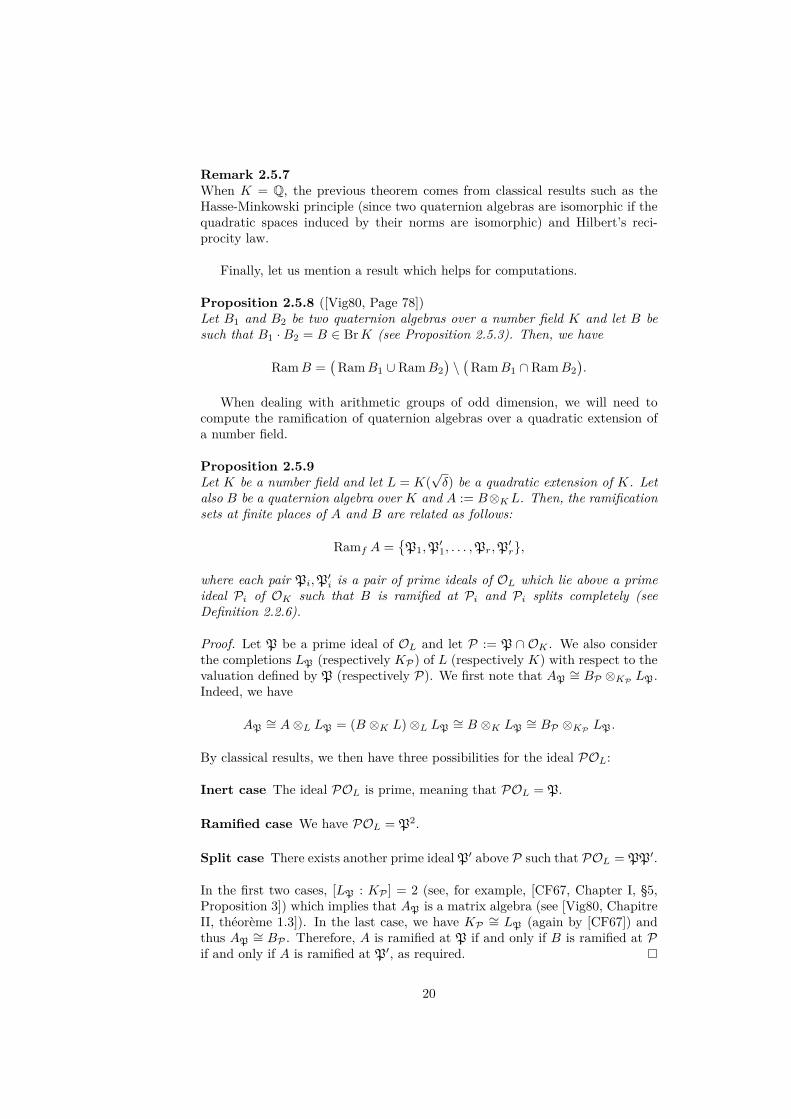
When dealing with arithmetic groups of odd dimension, we will need tocompute the ramification of quaternion algebras over a quadratic extension ofa number field.
Proposition 2.5.9Let K be a number field and let L = K(
√δ) be a quadratic extension of K. Let
also B be a quaternion algebra over K and A := B⊗KL. Then, the ramificationsets at finite places of A and B are related as follows:
Ramf A =P1,P
′1, . . . ,Pr,P
′r,
where each pair Pi,P′i is a pair of prime ideals of OL which lie above a prime
ideal Pi of OK such that B is ramified at Pi and Pi splits completely (seeDefinition 2.2.6).
Proof. Let P be a prime ideal of OL and let P := P ∩ OK . We also considerthe completions LP (respectively KP) of L (respectively K) with respect to thevaluation defined by P (respectively P). We first note that AP
∼= BP ⊗KP LP.Indeed, we have
AP∼= A⊗L LP = (B ⊗K L)⊗L LP
∼= B ⊗K LP∼= BP ⊗KP LP.
By classical results, we then have three possibilities for the ideal POL:
Inert case The ideal POL is prime, meaning that POL = P.
Ramified case We have POL = P2.
Split case There exists another prime idealP′ above P such that POL = PP′.
In the first two cases, [LP : KP ] = 2 (see, for example, [CF67, Chapter I, §5,Proposition 3]) which implies that AP is a matrix algebra (see [Vig80, ChapitreII, théorème 1.3]). In the last case, we have KP ∼= LP (again by [CF67]) andthus AP
∼= BP . Therefore, A is ramified at P if and only if B is ramified at Pif and only if A is ramified at P′, as required.
20
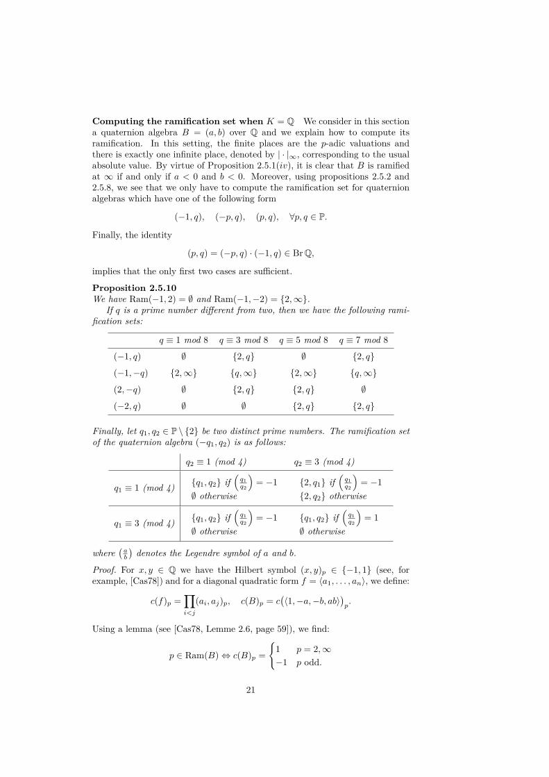
Computing the ramification set when K = Q We consider in this sectiona quaternion algebra B = (a, b) over Q and we explain how to compute itsramification. In this setting, the finite places are the p-adic valuations andthere is exactly one infinite place, denoted by | · |∞, corresponding to the usualabsolute value. By virtue of Proposition 2.5.1(iv), it is clear that B is ramifiedat ∞ if and only if a < 0 and b < 0. Moreover, using propositions 2.5.2 and2.5.8, we see that we only have to compute the ramification set for quaternionalgebras which have one of the following form
(−1, q), (−p, q), (p, q), ∀p, q ∈ P.
Finally, the identity
(p, q) = (−p, q) · (−1, q) ∈ BrQ,
implies that the only first two cases are sufficient.
Proposition 2.5.10We have Ram(−1, 2) = ∅ and Ram(−1,−2) = 2,∞.
If q is a prime number different from two, then we have the following rami-fication sets:
q ≡ 1 mod 8 q ≡ 3 mod 8 q ≡ 5 mod 8 q ≡ 7 mod 8
(−1, q) ∅ 2, q ∅ 2, q
(−1,−q) 2,∞ q,∞ 2,∞ q,∞
(2,−q) ∅ 2, q 2, q ∅
(−2, q) ∅ ∅ 2, q 2, q
Finally, let q1, q2 ∈ P \ 2 be two distinct prime numbers. The ramification setof the quaternion algebra (−q1, q2) is as follows:
q2 ≡ 1 (mod 4) q2 ≡ 3 (mod 4)
q1 ≡ 1 (mod 4) q1, q2 if(q1q2
)= −1
∅ otherwise2, q1 if
(q1q2
)= −1
2, q2 otherwise
q1 ≡ 3 (mod 4) q1, q2 if(q1q2
)= −1
∅ otherwiseq1, q2 if
(q1q2
)= 1
∅ otherwise
where(ab
)denotes the Legendre symbol of a and b.
Proof. For x, y ∈ Q we have the Hilbert symbol (x, y)p ∈ −1, 1 (see, forexample, [Cas78]) and for a diagonal quadratic form f = 〈a1, . . . , an〉, we define:
c(f)p =∏i<j
(ai, aj)p, c(B)p = c(〈1,−a,−b, ab〉
)p.
Using a lemma (see [Cas78, Lemme 2.6, page 59]), we find:
p ∈ Ram(B)⇔ c(B)p =
1 p = 2,∞−1 p odd.
21
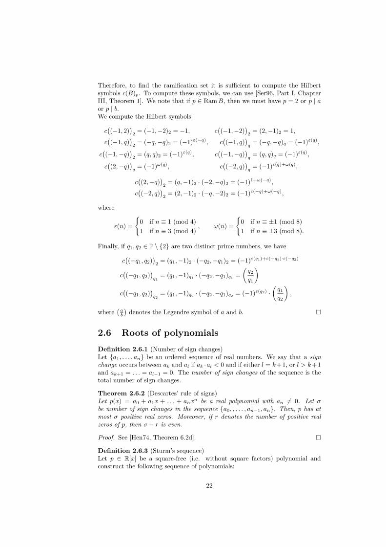
Therefore, to find the ramification set it is sufficient to compute the Hilbertsymbols c(B)p. To compute these symbols, we can use [Ser96, Part I, ChapterIII, Theorem 1]. We note that if p ∈ RamB, then we must have p = 2 or p | aor p | b.We compute the Hilbert symbols:
c((−1, 2)
)2 = (−1,−2)2 = −1, c
((−1,−2)
)2 = (2,−1)2 = 1,
c((−1, q)
)2 = (−q,−q)2 = (−1)ε(−q), c
((−1, q)
)q
= (−q,−q)q = (−1)ε(q),
c((−1,−q)
)2 = (q, q)2 = (−1)ε(q), c
((−1,−q)
)q
= (q, q)q = (−1)ε(q),
c((2,−q)
)q
= (−1)ω(q), c((−2, q)
)q
= (−1)ε(q)+ω(q),
c((2,−q)
)2 = (q,−1)2 · (−2,−q)2 = (−1)1+ω(−q),
c((−2, q)
)2 = (2,−1)2 · (−q,−2)2 = (−1)ε(−q)+ω(−q),
where
ε(n) =
0 if n ≡ 1 (mod 4)1 if n ≡ 3 (mod 4)
, ω(n) =
0 if n ≡ ±1 (mod 8)1 if n ≡ ±3 (mod 8).
Finally, if q1, q2 ∈ P \ 2 are two distinct prime numbers, we have
c((−q1, q2)
)2 = (q1,−1)2 · (−q2,−q1)2 = (−1)ε(q1)+ε(−q1)·ε(−q2)
c((−q1, q2)
)q1
= (q1,−1)q1 · (−q2,−q1)q1 =(q2
q1
)c((−q1, q2)
)q2
= (q1,−1)q2 · (−q2,−q1)q2 = (−1)ε(q2) ·(q1
q2
),
where(ab
)denotes the Legendre symbol of a and b.
2.6 Roots of polynomialsDefinition 2.6.1 (Number of sign changes)Let a1, . . . , an be an ordered sequence of real numbers. We say that a signchange occurs between ak and al if ak ·al < 0 and if either l = k+1, or l > k+1and ak+1 = . . . = al−1 = 0. The number of sign changes of the sequence is thetotal number of sign changes.
Theorem 2.6.2 (Descartes’ rule of signs)Let p(x) = a0 + a1x + . . . + anx
n be a real polynomial with an 6= 0. Let σbe number of sign changes in the sequence a0, , . . . , an−1, an. Then, p has atmost σ positive real zeros. Moreover, if r denotes the number of positive realzeros of p, then σ − r is even.
Proof. See [Hen74, Theorem 6.2d].
Definition 2.6.3 (Sturm’s sequence)Let p ∈ R[x] be a square-free (i.e. without square factors) polynomial andconstruct the following sequence of polynomials:
22

• p0(x) = p(x);
• p1(x) = p′(x);
• for k ≥ 2, we define pk as the opposite of the remainder of the polynomialdivision of pk−2 by pk−1, i.e. pk−2 = pk−1 ·qk−pk, with deg pk < deg pk−1;
The last polynomial pm of the sequence is the first constant polynomial. Then,we call p0, p1, . . . , pm a Sturm sequence for p.
Remarks 2.6.4 • The constant polynomial pm is non-zero if and only if pis square-free.
• The previous definition is in fact a particular case of a Sturm sequence.
Theorem 2.6.5 (Sturm’s theorem)Let p ∈ R[x] be a square-free polynomial and let p0, p1, . . . , pm be a Sturmsequence for p. For a real number λ ∈ R, we denote by σ(λ) the number ofsign changes in the sequence p0(λ), . . . , pm(λ). Let α < β be two real numberswhich are not roots of p. Then, the number of real zeros of p in the interval[a, b] is σ(α)− σ(β).
Proof. See [Hen74, Section 6.3].
Remark 2.6.6If we drop the assumption p(α) · p(β) 6= 0, then the result is the following: thenumber of real zeros in the interval (α, β] is given by σ(α)− σ(β).
Example 2.6.7A Sturm sequence of the polynomial p(x) = −4 + x − x2 + x3 is given by−4 + x− x2 + x3, 1− 2x+ 3x2, 35
9 −49x,−
341116 . We compute the sequences of
signs:
• for α = 0: −,+,+,−;
• for β = 1: +,+,+,−.
Therefore, p has 2− 1 = 1 real zero between 0 and 2.
Theorem 2.6.8Let p(x) = anx
n+an−1xn−1+. . .+a0 be a real polynomial with an 6= 0. Then, all
the real roots of p lie in the interval (−ρ, ρ), where ρ = 1+ 1|an| max0≤k≤n−1 |ak|.
Proof. See [RS02, Theorem 8.1.7].
2.7 Hilbert spacesDefinition 2.7.1 (Hilbert space)A Hilbert space is a real inner product space (H , 〈−,−〉) (not necessarily offinite dimension) such that H is complete with respect to the metric inducedby the inner product.
Definition 2.7.2 (Orthonormal basis of a Hilbert space)Let (H , 〈−,−〉) be a Hilbert space and let B = xi ⊂ H be a collectionof vectors of H . We say that B is an orthonormal Hilbert basis of H if thefollowing are satisfied:
23
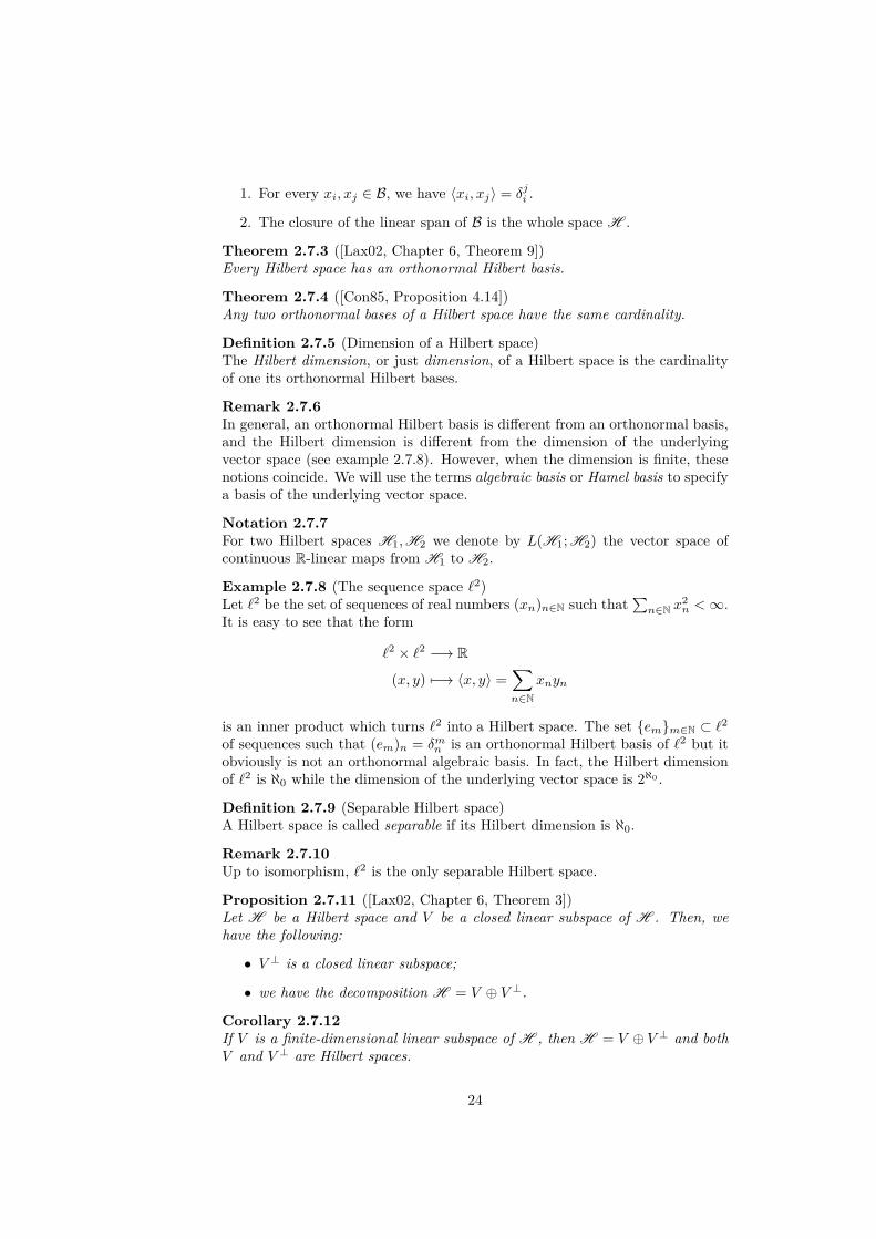
1. For every xi, xj ∈ B, we have 〈xi, xj〉 = δji .
2. The closure of the linear span of B is the whole space H .
Theorem 2.7.3 ([Lax02, Chapter 6, Theorem 9])Every Hilbert space has an orthonormal Hilbert basis.
Theorem 2.7.4 ([Con85, Proposition 4.14])Any two orthonormal bases of a Hilbert space have the same cardinality.
Definition 2.7.5 (Dimension of a Hilbert space)The Hilbert dimension, or just dimension, of a Hilbert space is the cardinalityof one its orthonormal Hilbert bases.
Remark 2.7.6In general, an orthonormal Hilbert basis is different from an orthonormal basis,and the Hilbert dimension is different from the dimension of the underlyingvector space (see example 2.7.8). However, when the dimension is finite, thesenotions coincide. We will use the terms algebraic basis or Hamel basis to specifya basis of the underlying vector space.
Notation 2.7.7For two Hilbert spaces H1,H2 we denote by L(H1; H2) the vector space ofcontinuous R-linear maps from H1 to H2.
Example 2.7.8 (The sequence space `2)Let `2 be the set of sequences of real numbers (xn)n∈N such that
∑n∈N x
2n <∞.
It is easy to see that the form
`2 × `2 −→ R
(x, y) 7−→ 〈x, y〉 =∑n∈N
xnyn
is an inner product which turns `2 into a Hilbert space. The set emm∈N ⊂ `2of sequences such that (em)n = δmn is an orthonormal Hilbert basis of `2 but itobviously is not an orthonormal algebraic basis. In fact, the Hilbert dimensionof `2 is ℵ0 while the dimension of the underlying vector space is 2ℵ0 .
Definition 2.7.9 (Separable Hilbert space)A Hilbert space is called separable if its Hilbert dimension is ℵ0.
Remark 2.7.10Up to isomorphism, `2 is the only separable Hilbert space.
Proposition 2.7.11 ([Lax02, Chapter 6, Theorem 3])Let H be a Hilbert space and V be a closed linear subspace of H . Then, wehave the following:
• V ⊥ is a closed linear subspace;
• we have the decomposition H = V ⊕ V ⊥.
Corollary 2.7.12If V is a finite-dimensional linear subspace of H , then H = V ⊕ V ⊥ and bothV and V ⊥ are Hilbert spaces.
24

Definition 2.7.13 (Tensor product of Hilbert spaces)Let (Hi, 〈−,−〉i), 1 ≤ i ≤ r, be a finite family of Hilbert spaces and considerthe usual tensor product (or algebraic tensor product) H := H1⊗ . . .⊗Hr. Wehave a natural bilinear form defined on simple tensors
(ei1 ⊗ . . .⊗ eir , e′i1 ⊗ . . .⊗ e
′ir
)7−→
r∏j=1〈eij , e′ij 〉, eij , e
′ij ∈Hj ,∀1 ≤ j ≤ r,
which extends by linearity to an inner product on H (see [Wei80, Section 3.4]).The completion of H with respect to the norm defined by this inner product isa Hilbert space which is denoted by H1⊗ . . . ⊗Hr.
Proposition 2.7.14Let H ,H ′ be two Hilbert spaces with their orthonormal Hilbert bases ei ande′j. Then, the collection ei⊗ e′j is an orthonormal Hilbert basis of H ⊗H ′.
Proof. See [Wei80, Theorem 3.12].
2.7.1 Geometry in Hilbert spacesLet (H , 〈−,−〉) be a Hilbert space. A unit vector a ∈ H and a scalar t ∈ Rdefine a hyperplane
P (a, t) =x ∈H : 〈a, x〉 = t
,
which in turn gives rise to the reflection with respect to P (a, t) given by
τ : H −→H
x 7−→ x+ 2(t− 〈a, x〉) · a.
The reflection extends naturally to a bijection of H := H ∪ ∞ by settingτ(∞) = ∞. In a similar way, a vector a ∈ H and a positive real number rdefine the sphere S(a, r) of radius r centered at a in the usual way, which inturn leads to the inversion with respect to S(a, r),
σ : H −→ H
x 7−→ a+(
r
d(x, a)
)2· (x− a),
(2.1)
with the convention that σ(a) =∞ and σ(∞) = a.
Definition 2.7.15 (Generalized sphere)A generalized sphere in H is either an extended hyperplane H = H ∪ ∞,where H is a hyperplane of H , or a sphere as above. If we want to emphasizeon the parameters, we will write Σ(a, r) for P (a, r) = P (a, r) ∪ ∞ or forS(a, r).
Definition 2.7.16 (Reflection in a generalized sphere)A reflection in a generalized sphere Σ is a reflection with respect to Σ if Σ is anextended hyperplane and an inversion in Σ if Σ is a sphere.
25

Definition 2.7.17The group of transformations whose elements are finite products of reflectionsin generalized spheres is denoted by Mob∗(H ).
Definition 2.7.18 (Similarity)Let y ∈H , T ∈ O(H ) and λ ∈ R∗+. The bijection of H to itself given by
x 7−→ λ · T (x) + y,
is called a similarity. The group of all similarities is denoted by Sim(H ); itcontains O(H ) as a subgroup.
Topology of H The collection of open subsets of H together with sets of theform ∞∪ (H \F ), where F is a bounded subset of H , defines a topology onH . Equipped with this topology, reflections with respect to generalized spheresare homeomorphisms of H to itself.
2.8 Riemannian manifoldsWe briefly present here the basic definitions which lead to the concept of aRiemannian manifold. A standard reference for this topic is [Kli95]. For thissection, we fix a Hilbert space H (note that H can be finite or infinite dimen-sional, separable or not).
Definition 2.8.1 (Topological manifold)LetM be a topological space. We say thatM is a topological manifold modelledon H , or just topological manifold if there is no ambiguity on H , ifM is locallyhomeomorphic to H .
Remarks 2.8.2 • Some authors require the underlying topological space ofa topological manifold to be separable and Hausdorff. In this case, theHilbert space H is separable and thus H ∼= `2.
• A topological manifold modelled on a Hilbert space is sometimes called aHilbert manifold.
Definition 2.8.3 (Differentiable map)Let U1 ⊂ H1 and U2 ⊂ H2 be two open subsets of two Hilbert spaces H1,H2and let f : U1 −→ U2 be a continuous map. We say that f is differentiable atu0 ∈ U1 if there exists dfu0 ∈ L(H1; H2) such that
f(u)− f(u0)− dfu0(u− u0) = o(|u− u0|).
The map is called differentiable of class C1 if it is differentiable at every u0 ∈ U1and if the map u 7−→ dfu is continuous. A map of class Ck is defined in asimilar way by induction. If f is of class Ck for every k ∈ N, we say that f isdifferentiable, or smooth.
Definition 2.8.4 (Diffeomorphism)A map f : U1 −→ U2 between two open subsets of two Hilbert spaces is a diffeo-morphism if it is differentiable, bijective and if its inverse is also differentiable.
26
Definition 2.8.5 (Differentiable atlas)Let M be a topological manifold modelled on H . A differentiable atlas for Mis a collection (ϕi, Ui)i∈I of charts which enjoys the following properties:
• Each Ui is an open set of M and the family Uii∈I is a covering of M .
• ϕi : Ui −→ ϕi(Ui) is a homeomorphism of Ui onto an open subset ϕi(Ui)of H .
• For every i, j ∈ I, the transition map
ϕi,j : ϕi(Ui ∩ Uj) −→ ϕj(Ui ∩ Uj), ϕi,j = ϕj ϕ−1i ,
is a diffeomorphism.
Definition 2.8.6 (Equivalent atlases)Two atlases of a topological manifold M are called equivalent if their union isan atlas of M .
Definition 2.8.7 (Differentiable structure)A differentiable structure on a topological manifold is an equivalence class ofdifferentiable atlases.
Definition 2.8.8 (Differentiable manifold)A differentiable manifold is a topological manifold modelled on a Hilbert spacetogether with a differentiable structure.
For a given differentiable manifold M and a point p ∈M , one can define thetangent space TpM at p as in the finite-dimensional case. This gives rise to thetangent bundle TM and leads to the definition of vector field. All the detailsare presented in [Kli95].
Definition 2.8.9 (Riemannian metric)A Riemannian metric g on a differentiable manifold M is a family of innerproducts
gp : TpM × TpM −→ R,such that for every pair of differentiable vector fields X,Y on M , the map
M −→ Rp 7−→ gp(Xp, Yp),
is differentiable.
Definition 2.8.10 (Riemannian manifold)A Riemannian manifold is a pair (M, g), where M is a differentiable manifoldand g is a Riemannian metric on M .
Remark 2.8.11We will often consider the Riemannian metric of a given Riemannian manifold asimplicitly given and write 〈v, w〉 for two vectors v, w ∈ TpM instead of gp(v, w).
Definition 2.8.12 (Conformal map)Let f : M −→ N be a diffeomorphism between two Riemannian manifolds. Themap f is called conformal, if there exists a differentiable map α : M −→ R∗+such that
〈dfp(v), dfp(w)〉 = α(p)2 · 〈v, w〉, ∀p ∈M, ∀v, w ∈ TpM.
27
Remark 2.8.13The above definition means that a conformal map should preserve angles be-tween curves meeting at a given point.
Example 2.8.14Reflections in generalized spheres and similarities are conformal maps.
In fact, the converse is also true: similarities, eventually composed with asphere inversion, are the only conformal maps of a real Hilbert space.
Theorem 2.8.15 (Liouville’s theorem)Let U ⊂ H be a connected open subset of a Hilbert space of dimension atleast 3 and let f : U −→ H be a conformal map. Then, one of the followingcases holds:
• There exist λ > 0, y ∈H and T ∈ O(H ) such that
f(z) = λ · T (z) + y, ∀z ∈ U.
• There exist λ > 0, x, y ∈H and T ∈ O(H ) such that
f(z) = λ · T(ιx(z)
)+ y, ∀z ∈ U,
where ιx is the inversion with respect to the sphere S(x, 1), as given byequation (2.1) of page 25.
Proof. See [Huf76].
The previous theorem implies that every conformal map f : U −→ H ,where U is an open connected subset of H , can be extended in a unique wayto a homeomorphism f : H −→ H , where H := H ∪ ∞.
Definition 2.8.16 (Möbius transformation, Möbius group)The map f is called a Möbius transformation. The group of all Möbius transfor-mations of a Hilbert space H is called the Möbius group of H and is denotedby Mob(H ).
Remark 2.8.17When the dimension of the Hilbert space is finite, a Möbius transformation is thecomposition of a finite number of reflections in generalized spheres (see [Rat06,§4.3] for example). However, when the dimension of the space is infinite, someelements of Mob(H ) cannot be written as a finite composition of inversions.Indeed, a map of type f(z) = λ · T
(ιx(z)
)+ y or f(z) = λ · T (z) + y can be
written as a finite product of reflections in generalized spheres if and only if thespace of fixed points of T has finite codimension. In other words, Mob∗(H ) (seeDefinition 2.7.17) is a proper subgroup of Mob(H ) if H is infinite-dimensional.
28

CHAPTER 3Hyperbolic space, Coxeter groups and Coxeter
polyhedra
In this chapter, we present the theoretical background related to hyperbolicspace, reflection groups and polyhedra. In the first section, we introduce dif-ferent models for the three simply connected complete Riemannian manifoldsXn of constant sectional curvature +1, 0, and −1. Concerning the hyperbolicspace, we also explain how the classical models can be extended to the infinite-dimensional setting. The finite-dimensional case is treated in details in [Rat06]while its infinite-dimensional counterpart is presented in [Das12]1. Finally, wealso present well-known general facts about isometries of the hyperbolic space,especially in the upper half-space model.
Concerning Coxeter groups, we first give the abstract definition before re-stricting ourselves to geometric Coxeter groups, that is, Coxeter groups whichare realized as discrete subgroups generated by finitely many reflections in hy-perplanes of Xn.
Finally, we present various invariants of hyperbolic Coxeter groups (growthseries and growth rate, Euler characteristic, cocompactness and cofiniteness, f -vector, arithmeticity) and explain how we can compute these invariants. Allthese computations are implemented in my computer program CoxIter, whichis presented in Chapter 5.
3.1 Three geometries and their models
It is well known that there exist only three simply connected complete Rieman-nian manifolds of constant sectional curvature of dimension n ≥ 2: the spheresSn, the Euclidean spaces En and the hyperbolic spaces Hn. Up to a rescaling ofthe metric, we can suppose that the curvatures are respectively +1, 0 and −1.We will write X, or Xn if we want to emphasize on the dimension, for one of thethree spaces.
For ε = +1, 0,−1, we consider Rn+1 equipped with the bilinear form given
1Although only the separable case is treated in [Das12], the results we need also work forany infinite-dimensional hyperbolic space (i.e. not necessarily separable).
29

by
〈−,−〉ε : Rn+1 × Rn+1 −→ R
(x, y) 7−→n∑i=1
xiyi + ε · xn+1yn+1.
Recall that the form 〈−,−〉−1 is often called Lorentzian form. We can nowdefine the models for our geometries. The n-dimensional sphere Sn is definedto be the set
Sn = x ∈ Rn+1 : 〈x, x〉1 = 1,
together with the distance function d = dSn given by
cos d(x, y) = 〈x, y〉1, ∀x, y ∈ Sn.
The n-Euclidean space En can be identified with the set
En = x ∈ Rn+1 : xn+1 = 0,
endowed with the metric given by
d(x, y) = dEn(x, y) =√〈x, y〉0, ∀x, y ∈ Rn+1.
The hyperboloid model, or vector space model, of the hyperbolic n-space Hnarises as the set
Hn = x ∈ Rn+1 : 〈x, x〉−1 = −1, xn+1 > 0, (3.1)
together with the distance defined by the relation
d(x, y) = dHn(x, y) = arcosh(−〈x, y〉−1), ∀x, y ∈ Hn.
The volume element is given by
dx1 · . . . · dxn√1 + x2
1 + . . .+ x2n
,
as shown in [Rat06, Theorem 3.4.1]. The boundary of Hn can be identified withthe set
∂Hn =x ∈ Rn+1 : 〈x, x〉−1 = 0,
n+1∑i=1
x2i = 1, xn+1 ≥ 0
,
and we let Hn := ∂Hn∪Hn. A hyperplane of Hn is given by the intersection ofthe orthogonal complement (with respect to the Lorentzian product) of a vectorv of Lorentzian norm 1 and Hn. We denote such a hyperplane by Hv. Remarkthat such a hyperplane splits Hn into two half-spaces H+
v :=x ∈ Hn : 〈v, x〉 ≥
0and H−v :=
x ∈ Hn : 〈v, x〉 ≤ 0
whose intersection is Hv. The relative
behaviour of two distinct hyperplanes Hv and Hw can be described by means ofthe Lorentzian product of v and w (see [Rat06, Theorems 3.2.6, 3.2.7 and 3.2.9]or [Vin85, Section 1.1]):
• The hyperplanes intersect if and only if |〈v, w〉| < 1. In this case, theacute dihedral angle in
(0, π2
]between them is given by arccos(|〈v, w〉|).
30

• The hyperplanes are parallel if and only if |〈v, w〉| = 1. In this case theirdihedral angle is 0.
• The hyperplanes are ultraparallel if and only if |〈v, w〉| > 1. In thissetting, the two hyperplanes admit a common perpendicular of lengtharcosh(|〈v, w|〉).
3.2 Models of the hyperbolic spaceIn this section, we present two other models of the hyperbolic space, the upperhalf-space model and the Poincaré ball model, together with a different versionof the hyperboloid model. We adopt an approach that allows us to define modelswhich are both finite and infinite-dimensional. We use the notation Hn to denoteany of the three models Un, Hn and Bn. We also describe the isometries of theupper half-space model.
We consider a Hilbert space (H , 〈−,−〉H ) of Hilbert dimension n (see Def-inition 2.7.5) and some unit vector u ∈ H . By Corollary 2.7.12, we have adecomposition of H as a direct sum of Hilbert space, that is H = 〈u〉⊥ ⊕ 〈u〉and this decomposition comes with the projection π〈u〉⊥ of H onto 〈u〉⊥ andthe functional lu defined as follows:
lu : H −→ Rx 7−→ 〈x, u〉H .
3.2.1 The upper half-space modelWe consider the set
Un = UH = x ∈H : lu(x) > 0,
together with the distance function given by
d(x, y) = dUn(x, y) = arcosh(
1 + dH (x, y)2 · lu(x) · lu(y)
), ∀x, y ∈ Un.
We call Un the upper half-space model of the hyperbolic n-space. The boundaryUn is given by
∂Un =x ∈H : lu(x) = 0
∪ ∞.
Remarks 3.2.1 • The upper half-space model is suitable to get isometriesfrom 2× 2 Clifford matrices. We will come back to this question in Chap-ter 8.
• If H = Rn and u = en, the above construction gives the usual upperhalf-space model Un (see [Rat06, §4.6]).
• When H = `2 (see Example 2.7.8), we usually take u = (1, 0, . . .).
• If the dimension of H is infinite, we will often discard the cardinal n andonly write U∞.
31

3.2.2 The hyperboloid modelWe define on the product R×H the bilinear form
B((λ, x), (µ, y)
)= 〈x, y〉H − λµ,
and we consider its associated quadratic form q. ThenHn = HH =
(λ, x) ∈ R×H : q(λ, x) = ‖x‖2H − λ2 = −1, λ > 0
,
together with the distance function defined byd = dHn = arcosh
(−B
((λ, x), (µ, y)
)), ∀(λ, x), (µ, y) ∈ Hn.
We call Hn the hyperboloid model, or the vector space model, of the hyperbolicn-space in R×H .Remarks 3.2.2 • The hyperboloid model is suitable to define and treat hy-
perplanes in terms of linear subspaces.
• If H = Rn, the above construction gives the classical hyperboloid modelHn presented above (see equation (3.1) on page 63 and [Rat06, §3.2]).
• As for the upper half-space model, if the dimension of H is infinite, wewill often discard the cardinal n and write only H∞.
• Another standard way to construct Hn is to look at the quotient C/R∗,where C is the cone
(λ, x) ∈ Hn : q(λ, x) < 0
. Then, the distance d on
C given by
cosh2 d(x, y) = B(x, y)2
q(x) · q(y) , ∀x, y ∈ C,
induces a distance on C/R∗.
• The space R×H , together with the quadratic form (λ, x) 7−→ ‖x‖2−λ2,is a quadratic space of index 1 (see [BIM05] for the definition). Moreover,the space Hn is a geodesic CAT(−1) space (see [BIM05, Proposition 4.2]).
3.2.3 Poincaré ball modelWe consider the set
Bn = BH =x ∈H : ‖x‖H < 1
,
together with the distance function given by
dBn(x, y) = arcosh(
1 + 2 · dH (x, y)(1− ‖x‖2H
)·(1− ‖y‖2H
)) , ∀x, y ∈ Bn.
We call Bn the Poincaré ball model of the hyperbolic n-space. Its boundary isgiven by
∂Bn = x ∈H : ‖x‖H = 1.Remarks 3.2.3 • When the dimension of H is finite, the Poincaré ball
model is suitable to visualize non-compact polyhedra.
• If H = Rn, the above construction gives the usual Poincaré ball model(see [Rat06, §4.5]).
• If the dimension of H is infinite, we will often discard the cardinal n andwrite only B∞.
32

3.2.4 Models of the hyperbolic space as Riemannian man-ifolds
As in the finite dimensional case, the models Un and Hn of the hyperbolic spacecan be viewed as Riemannian manifolds (see Definition 2.8.10). The Riemannianmetric at a point p ∈ Hn are given in the next table.
Model Riemannian metric
Un gp(v, w) = 〈v, w〉Hlu(p)2 , ∀v, w ∈ Tp Un ∼= H
Hn gp((λ, x), (µ, y)
)= −λ · µ+ 〈x, y〉H , ∀(λ, x), (µ, y) ∈ TpHn
Bn gp(v, w) = 4 · 〈v, w〉H(1− ‖x‖2H
)2 , ∀v, w ∈ TpBn ∼= H
Note that the tangent space TpHn at a point p = (ν, z) ∈ Hn is given by
TpHn =
(λ, x) ∈ R×H : B((ν, z), (λ, x))
)= 〈z, x〉H − νλ = 0
.
3.2.5 Isometries of the upper half-spaceReflections in generalized spheres and similarities (see Section 2.7.1) of a codi-mension 1 subspace in H can be used to define isometries of the hyperbolic spaceas follows. We consider the decomposition H = 〈u〉⊥ ⊕ 〈u〉, where u ∈ H isa unit vector, and the associated upper half-space model U = UH = x ∈ H :lu(x) > 0. Now, if Σ(a, r) is a generalized sphere in the Hilbert space 〈u〉⊥with associated reflection σ, then Σ(a+ 0, r) is a generalized sphere of H withassociated reflection σ in a natural way. On the other hand, if
η : 〈u〉⊥ −→ 〈u〉⊥, x 7−→ λ · T (x) + y
is a similarity (see Definition 2.7.18) of 〈u〉⊥, then we have an induced similarityη of H given by
η : H −→H , x 7−→ λ ·(T (π〈u〉⊥(x)) + π〈u〉(x)
)+ y,
where πV denotes the projection onto the subspace V of H . It is easily shownthat these induced maps are isometries of the space Un.
Definition 3.2.4 (Poincaré extension)For a reflection σ in a generalized sphere of 〈u〉⊥ (respectively a similarity η ∈Sim(〈u〉⊥)), the induced bijection σ (respectively η) of H is called the Poincaréextension of σ (respectively η).
Remark 3.2.5In a similar way, if V is any subspace of H and if ϕ is an element of Mob(V ),then ϕ can be extended via Poincaré extension to an element of Mob(H ).
The following result provides an important characterisation of isometries ofthe upper half-space.
33

Theorem 3.2.6Let g : Un −→ Un be a diffeomorphism. Then, the following are equivalent:
1. g is a conformal isomorphism of Un.
2. g extends to a Möbius transformation g ∈ Mob(H ) which preserves Un.
3. g preserves the Riemannian metric of Un.
4. g is an isometry of Un, that is,
dUn
(g(x), g(y)
)= dUn(x, y), ∀x, y ∈ Un.
Proof. The proof given in [Das12, Theorem 2.15] also works in the non-separablecase.
Remark 3.2.7To avoid cumbersome notations, we will often use the same notation for anisometry g : Un −→ Un and its Möbius extension g : H −→H .
If V is any closed subspace of 〈u〉⊥ and if g is a similarity of V , then thePoincaré extension g : H −→ H will preserve the upper half-space Un, whichmeans that the restriction of g to Un is an isometry. Reciprocally, if g is anisometry of Un, then the extension g : H −→H preserves ∂Un = 〈u〉⊥ ∪ ∞.Therefore, g
∣∣∂Un is an element of Mob(∂Un) whose Poincaré extension is g. In
other words, we have the following corollary.
Corollary 3.2.8The group of isometries Isom(Un) is isomorphic to the group Mob(〈u〉⊥).
We have the following analogous result for the group Mob∗.
Corollary 3.2.9If g : Un −→ Un is an isometry of Un whose Möbius extension g can be writtenas a composition of a finite number of reflections in generalized spheres (i.e. wehave g ∈ Mob∗(H )), then there exists a finite-dimensional subspace V of 〈u〉⊥and an element ϕ ∈ Mob(V ) such that the Poincaré extension of ϕ to H isequal to g.
Remark 3.2.10We will see in Chapter 8 that the isometries arising as a finite composition ofreflections in generalized spheres are exactly the isometries coming from Cliffordmatrices.
3.2.5.1 Classification of isometries
Any isometry of Hn can be represented as an isometry of the ball model g :Bn −→ Bn and this isometry can be extended in a unique way to a continuousbijective map g : Bn −→ Bn. This extension has (at least) one fixed point bythe Brouwer fixed point theorem (or the Schauder fixed point theorem in theinfinite-dimensional setting). Then, the isometry g is said to be
1. elliptic if g has a fixed point in Bn;
2. parabolic if g has exactly one fixed point in ∂Bn and no fixed point in Bn;
34

3. loxodromic, if g has exactly two fixed points in ∂Bn and no fixed point inBn.
We notice that this definition is independent of the conjugacy class of g. More-over, the same classification can be done independently of the model. Therefore,we will call an isometry g : Hn −→ Hn
1. elliptic if g has a fixed point in Hn;
2. parabolic if g has exactly one fixed point in ∂Hn and no fixed point in Hn;
3. loxodromic, or hyperbolic, if g has exactly two fixed points in ∂Hn and nofixed point in Hn.
There is some work to be done to show that these three possibilities are mutuallyexclusive and that any isometry of Hn falls into precisely one of this three cases;we refer to [Das12, §2.7] for the proof and some details. Finally, we have thefollowing explicit characterization of isometries.
Proposition 3.2.11 ([Das12, Proposition 2.30])Let g ∈ IsomHn be an isometry of the hyperbolic space Hn. Then, g is conjugateto exactly one of the following:
• An isometry of Bn coming from an isometry T of O(H ). This is theelliptic case.
• An isometry of Un coming from a Möbius transformation x 7→ T (x) + y,with y 6= 0 and T ∈ O(H ). This corresponds to the parabolic case.
• An isometry of Un coming from a Möbius transformation x 7→ λT (x), withT ∈ O(H ) and λ > 0, λ 6= 1. This corresponds to the loxodromic case.
Proposition 3.2.12Let g be a parabolic isometry of the hyperbolic space Un and suppose that g isconjugate to the map ϕ : x 7−→ T (x) + y, with T ∈ O(H ) (see Proposition3.2.11) and some y ∈ H . If the space Fix T of fixed points of T has finitecodimension (or equivalently if T can be written as a finite composition of re-flections), then one can suppose that y ∈ Fix T .
Proof. Since T is continuous, the set Fix T is a closed subspace of H . Thus,Proposition 2.7.11 implies that we have the decomposition H = Fix T ⊕ C,with C := (Fix T )⊥. Now, we can write y = f + c with f ∈ Fix T and c ∈C. Moreover, since the restriction of T − id to C is injective, and since C isfinite dimensional, then there exists c′ ∈ C such that (T − id)(c′) = c. As aconsequence, the conjugate τ ϕ τ−1, with τ(x) = x+ c′, sends x to T (x) + f ,as required.
3.3 Abstract Coxeter groupsDefinition 3.3.1 (Coxeter group)A Coxeter group is a finitely presented group generated by elements s1, . . . , sdand such that
〈s1, . . . , sd : (si sj)mij = 1〉,
35

where mij = 1 if and only if i = j, and mij = mji ∈ 2, 3, . . . ∪ ∞ if i 6= j.By mij =∞, we mean that there is no relation between si and sj . If Γ is sucha group and S := s1, . . . , sd is the set of generators, we will refer to the groupas (Γ, S), or just Γ if there is no ambiguity on S. When it is convenient, we usethe notation m(si, sj) := mij .If S′ is a subset of S, we denote by ΓS′ the subgroup of Γ generated by theelements of S′.
Definition 3.3.2 (Coxeter graph of a Coxeter group)An easy way to represent a Coxeter group
(Γ, S = s1, . . . , sd
)is by its Coxeter
diagram, or Coxeter graph. The Coxeter diagram of Γ is the graph whose verticescorrespond to the elements of S. Moreover, there is an edge between the verticessi and sj if and only if m(si, sj) ≥ 3. We label such an edge with m(si, sj) ifm(si, sj) ≥ 4. Sometimes, instead of labelling the edge, we use a double edge ifm(si, sj) = 4 and a bold (or heavy) edge if m(si, sj) =∞.
Examples 3.3.3 • It is well known that the symmetric group Sn is isomor-phic to the Coxeter group An−1 (see Figure 3.1): the ith node of An−1corresponds to the transposition (i, i+ 1) of Sn.
• The dihedral group of 2m elements is isomorphic to G(m)2 (see Figure 3.1).
• If P is a polyhedron (see Definition 3.4.1) in the affine space Rn whosedihedral angles are integer submultiples of π and if Γ < IsomRn is the(discrete) group generated by the reflections in the facets of P , then Γ isa Coxeter group.
Definition 3.3.4 (Irreducible Coxeter group)A Coxeter group is said to be irreducible if its Coxeter diagram is connected.
It is easy to see that a Coxeter group is the product of the groups corre-sponding to the connected components of its Coxeter diagram. Moreover, thefinite irreducible Coxeter groups were classified by Coxeter [Cox35] by means oftheir Coxeter diagrams. The classification is presented in Figure 3.1.
Figure 3.1 – Irreducible finite Coxeter groups
3.4 Geometric Coxeter groupsIn this section, we present the connection between abstract Coxeter groups anddiscrete reflection groups in the facets (sides of codimension 1) of convex finite-sided polyhedra. The main reference is [Rat06, §7.1]. In what follows, X denotesthe unit n-sphere Sn, the Euclidean n-space En or Hn.
36
A vector v ∈ En and a real number t ∈ R determine an (affine) hyperplaneHv,t := x ∈ En : 〈x, v〉 = t, denoted Hv if t = 0, and such a hyperplane splitsEn in two half-spaces H+
v,t :=x ∈ En : 〈v, x〉 ≥ t
and H−v,t :=
x ∈ En :
〈v, x〉 ≤ twhose intersection is Hv,t. A hyperplane in Sn is the intersection
of a hyperplane Hv of En+1 with Sn. Similarly, we saw in Section 3.1 that ahyperplane of Hn is the intersection of a hyperplane of En with Hn.
Definition 3.4.1 (Polyhedron)A polyhedron P in X is a subset of X which is the intersection of finitely manyhalf-spaces, each one bounded by a hyperplane. Moreover, we require that Phas non-empty interior and that no half-space contains the intersection of theothers.
Definition 3.4.2 (Reflection with respect to a hyperplane)Let Hv be a hyperplane of X. The reflection rv = rHv associated to the hyper-plane Hv is defined as follows (recall that we choose v with norm 1):
rHv : X −→ X
x 7−→ x− 2〈x, v〉v.
Definition 3.4.3 (Reflection group associated to a polyhedron)Let P =
⋂di=1H
−vi be a polyhedron in X and Γ ≤ IsomX. We say that Γ is the
reflection group associated to P if Γ is generated by the reflections in the facetsof P , that is Γ = 〈rHv1 , . . . , rHvd 〉.
Definition 3.4.4 (Cell of a group generated by reflections)Let Γ < IsomX be a discrete group generated by reflections. The hyperplanescorresponding to all reflections of Γ decompose X into convex polyhedra calledcells of Γ.
Remark 3.4.5Of course, Γ acts transitively on the set of its cells. Moreover, each cell is theclosure of a fundamental region for Γ.
Let Γ ≤ IsomX be a discrete reflection group with respect to a polyhedronP ⊂ X (i.e. P is a cell for Γ, Γ is generated by reflections in the sides of Pand Γ is discrete). Then, all the dihedral angles of P are submultiples of π (i.e.0 or of the form π/k where k ∈ N, k ≥ 2). For any facet Si of P , we let Hvi
be the hyperplane containing Si such that P ⊂ H−vi . Now, if the dihedral anglebetween two adjacent facets Si and Sj of P is π/θ(Si, Sj), then the order ofrvi rvj in Γ is θ(Si, Sj) (see [Rat06, Theorem 7.1.2]). Suppose now that P isof finite volume and has facets S = S1, . . . , Sd. Then, by [Rat06, Theorem7.1.4] we have
〈r1, . . . , rd|r2i = 1, (ri · rj)θ(Si,Sj) = 1〉 ∼= Γ.
This motivates the following definition.
Definition 3.4.6 (Geometric Coxeter group)A Coxeter group Γ is a geometric Coxeter group if there exists a polyhedronP ⊂ X, where X = Sn, En,Hn, such that Γ is the associated reflection groupof P .
37
Definition 3.4.7 (Gram matrix)Let Γ < IsomX be a geometric Coxeter group and let P =
⋂ri=1H
−vi be its
corresponding polyhedron. The Gram matrix of the polyhedron P ⊂ X, or theGram matrix of the geometric Coxeter group Γ, is the matrix G = G(P ) =G(Γ) ∈ Mat(r;R) defined as G =
(〈vi, vj〉
)1≤i,j≤r.
If we are given the matrix G = G(Γ) of a geometric Coxeter group Γ, wecan find the space on which Γ acts as follows. The matrix G = G(Γ) inducesa quadratic form called the Tits form on Rd, where d = |S|, via x 7−→ xtGx.If the matrix G is indecomposable (meaning that we cannot transform G toa block diagonal matrix with permutations of the rows and columns of G) or,equivalently, if the graph of the group is connected, then we get informationabout the group by looking at the signature (n, p, q) of the quadratic form,where n (respectively p, q) is the number of positive (respectively negative,zero) eigenvalues of G. For positive n, we are interested in the following cases:
p = q = 0 (the quadratic form is positive definite) In this case, the group is finite(see the classification of irreducible finite Coxeter groups in Figure 3.1).It can be shown that Γ can be realized as a discrete group of isometriesof the n-sphere Sn. Thus, Γ is called spherical.
p = 0, q > 0 (the quadratic form is positive semidefinite) The group can be re-alized as a discrete subgroup of IsomEn. Hence, it is said to be affine(or Euclidean or parabolic). The classification of irreducible affine Coxetergroups is given in Figure 3.2 (see, for example, [Bou68a, Chapter 6, §4.3,Theorem 4]).
p = 1, q ≥ 0 The group can be realized as a discrete subgroup of IsomHn (seedetails in Section 3.5). Thus, it is called hyperbolic.
Now, if the matrix G is decomposable to a diagonal block matrix with blocksG1, . . . , Gl, we say that the group is spherical (respectively affine) if each blockGi is spherical (respectively affine). If the matrix G has signature (n, 1, q) forsome n and q, we say that the group is hyperbolic.If G is the Coxeter diagram of Γ, then a subdiagram of G is called spherical(respectively affine, hyperbolic) if the corresponding subgroup of Γ is spherical(respectively affine, hyperbolic).
3.5 Hyperbolic Coxeter groups and hyperbolicCoxeter polyhedra
In this section, we present some concepts related to hyperbolic Coxeter groupsand polyhedra. Let P ⊂ Hn be a polyhedron. Hence, there exist vectorsv1, . . . , vr of Lorentzian norm 1 and hyperplanes Hi = 〈vi〉⊥ such that P =⋂ri=1H
−i , where H−i is the half-space delimited by Hi and given by H−i :=
x ∈ Hn : 〈x, vi〉 ≤ 0.
Remark 3.5.1Unlike in the Euclidean space, there exist unbounded hyperbolic Coxeter poly-hedra of finite volume. Such a polyhedron is the convex hull of a finite set ofpoints x1, . . . , xk ∈ Hn with at least one xi ∈ ∂Hn. Such a vertex is called a
38
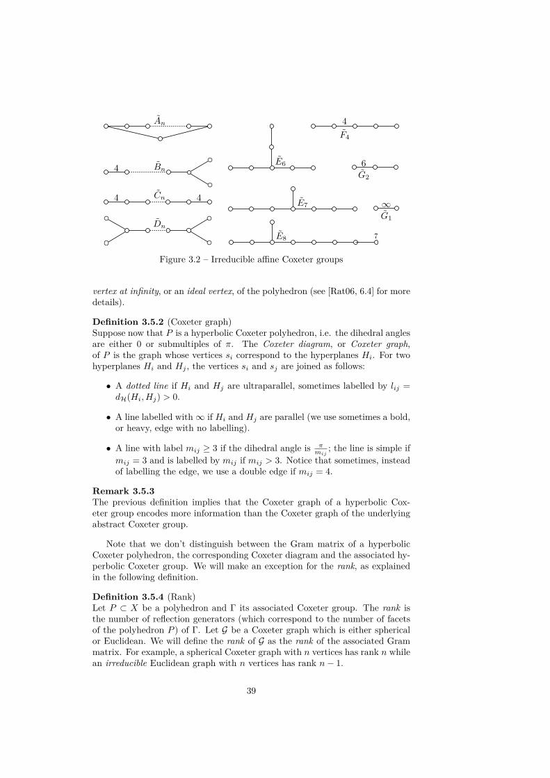
Figure 3.2 – Irreducible affine Coxeter groups
vertex at infinity, or an ideal vertex, of the polyhedron (see [Rat06, 6.4] for moredetails).
Definition 3.5.2 (Coxeter graph)Suppose now that P is a hyperbolic Coxeter polyhedron, i.e. the dihedral anglesare either 0 or submultiples of π. The Coxeter diagram, or Coxeter graph,of P is the graph whose vertices si correspond to the hyperplanes Hi. For twohyperplanes Hi and Hj , the vertices si and sj are joined as follows:
• A dotted line if Hi and Hj are ultraparallel, sometimes labelled by lij =dH(Hi, Hj) > 0.
• A line labelled with∞ if Hi and Hj are parallel (we use sometimes a bold,or heavy, edge with no labelling).
• A line with label mij ≥ 3 if the dihedral angle is πmij
; the line is simple ifmij = 3 and is labelled by mij if mij > 3. Notice that sometimes, insteadof labelling the edge, we use a double edge if mij = 4.
Remark 3.5.3The previous definition implies that the Coxeter graph of a hyperbolic Cox-eter group encodes more information than the Coxeter graph of the underlyingabstract Coxeter group.
Note that we don’t distinguish between the Gram matrix of a hyperbolicCoxeter polyhedron, the corresponding Coxeter diagram and the associated hy-perbolic Coxeter group. We will make an exception for the rank, as explainedin the following definition.
Definition 3.5.4 (Rank)Let P ⊂ X be a polyhedron and Γ its associated Coxeter group. The rank isthe number of reflection generators (which correspond to the number of facetsof the polyhedron P ) of Γ. Let G be a Coxeter graph which is either sphericalor Euclidean. We will define the rank of G as the rank of the associated Grammatrix. For example, a spherical Coxeter graph with n vertices has rank n whilean irreducible Euclidean graph with n vertices has rank n− 1.
39
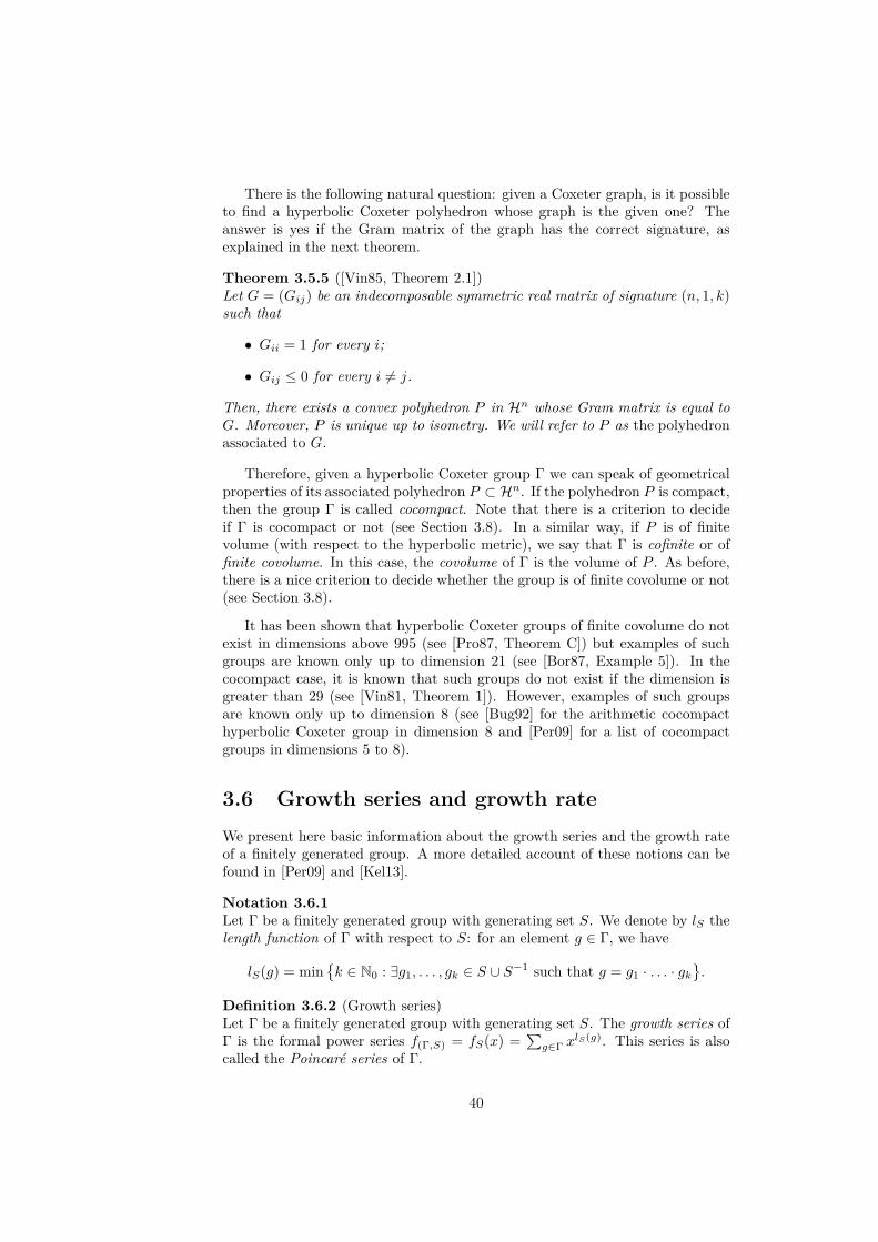
There is the following natural question: given a Coxeter graph, is it possibleto find a hyperbolic Coxeter polyhedron whose graph is the given one? Theanswer is yes if the Gram matrix of the graph has the correct signature, asexplained in the next theorem.
Theorem 3.5.5 ([Vin85, Theorem 2.1])Let G = (Gij) be an indecomposable symmetric real matrix of signature (n, 1, k)such that
• Gii = 1 for every i;
• Gij ≤ 0 for every i 6= j.
Then, there exists a convex polyhedron P in Hn whose Gram matrix is equal toG. Moreover, P is unique up to isometry. We will refer to P as the polyhedronassociated to G.
Therefore, given a hyperbolic Coxeter group Γ we can speak of geometricalproperties of its associated polyhedron P ⊂ Hn. If the polyhedron P is compact,then the group Γ is called cocompact. Note that there is a criterion to decideif Γ is cocompact or not (see Section 3.8). In a similar way, if P is of finitevolume (with respect to the hyperbolic metric), we say that Γ is cofinite or offinite covolume. In this case, the covolume of Γ is the volume of P . As before,there is a nice criterion to decide whether the group is of finite covolume or not(see Section 3.8).
It has been shown that hyperbolic Coxeter groups of finite covolume do notexist in dimensions above 995 (see [Pro87, Theorem C]) but examples of suchgroups are known only up to dimension 21 (see [Bor87, Example 5]). In thecocompact case, it is known that such groups do not exist if the dimension isgreater than 29 (see [Vin81, Theorem 1]). However, examples of such groupsare known only up to dimension 8 (see [Bug92] for the arithmetic cocompacthyperbolic Coxeter group in dimension 8 and [Per09] for a list of cocompactgroups in dimensions 5 to 8).
3.6 Growth series and growth rateWe present here basic information about the growth series and the growth rateof a finitely generated group. A more detailed account of these notions can befound in [Per09] and [Kel13].
Notation 3.6.1Let Γ be a finitely generated group with generating set S. We denote by lS thelength function of Γ with respect to S: for an element g ∈ Γ, we have
lS(g) = mink ∈ N0 : ∃g1, . . . , gk ∈ S ∪ S−1 such that g = g1 · . . . · gk
.
Definition 3.6.2 (Growth series)Let Γ be a finitely generated group with generating set S. The growth series ofΓ is the formal power series f(Γ,S) = fS(x) =
∑g∈Γ x
lS(g). This series is alsocalled the Poincaré series of Γ.
40
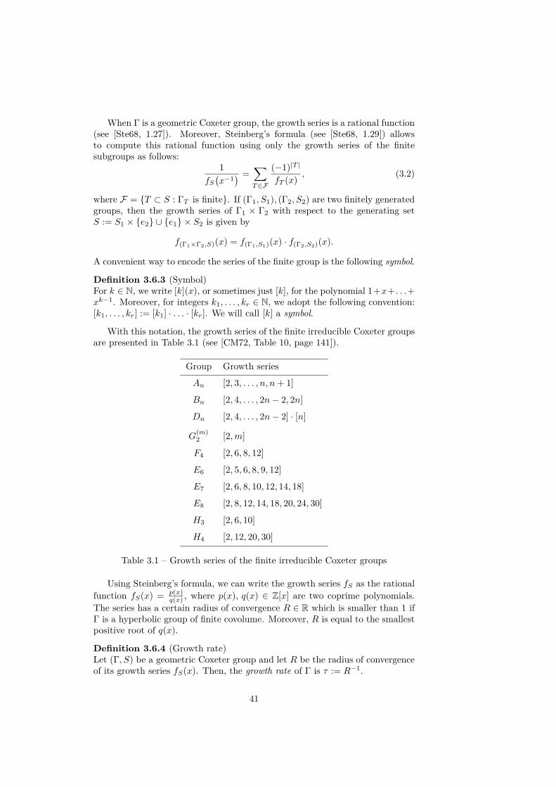
When Γ is a geometric Coxeter group, the growth series is a rational function(see [Ste68, 1.27]). Moreover, Steinberg’s formula (see [Ste68, 1.29]) allowsto compute this rational function using only the growth series of the finitesubgroups as follows:
1fS(x−1
) =∑T∈F
(−1)|T |
fT (x) , (3.2)
where F = T ⊂ S : ΓT is finite. If (Γ1, S1), (Γ2, S2) are two finitely generatedgroups, then the growth series of Γ1 × Γ2 with respect to the generating setS := S1 × e2 ∪ e1 × S2 is given by
f(Γ1×Γ2,S)(x) = f(Γ1,S1)(x) · f(Γ2,S2)(x).
A convenient way to encode the series of the finite group is the following symbol.
Definition 3.6.3 (Symbol)For k ∈ N, we write [k](x), or sometimes just [k], for the polynomial 1+x+ . . .+xk−1. Moreover, for integers k1, . . . , kr ∈ N, we adopt the following convention:[k1, . . . , kr] := [k1] · . . . · [kr]. We will call [k] a symbol.
With this notation, the growth series of the finite irreducible Coxeter groupsare presented in Table 3.1 (see [CM72, Table 10, page 141]).
Group Growth series
An [2, 3, . . . , n, n+ 1]
Bn [2, 4, . . . , 2n− 2, 2n]
Dn [2, 4, . . . , 2n− 2] · [n]
G(m)2 [2,m]
F4 [2, 6, 8, 12]
E6 [2, 5, 6, 8, 9, 12]
E7 [2, 6, 8, 10, 12, 14, 18]
E8 [2, 8, 12, 14, 18, 20, 24, 30]
H3 [2, 6, 10]
H4 [2, 12, 20, 30]
Table 3.1 – Growth series of the finite irreducible Coxeter groups
Using Steinberg’s formula, we can write the growth series fS as the rationalfunction fS(x) = p(x)
q(x) , where p(x), q(x) ∈ Z[x] are two coprime polynomials.The series has a certain radius of convergence R ∈ R which is smaller than 1 ifΓ is a hyperbolic group of finite covolume. Moreover, R is equal to the smallestpositive root of q(x).
Definition 3.6.4 (Growth rate)Let (Γ, S) be a geometric Coxeter group and let R be the radius of convergenceof its growth series fS(x). Then, the growth rate of Γ is τ := R−1.
41
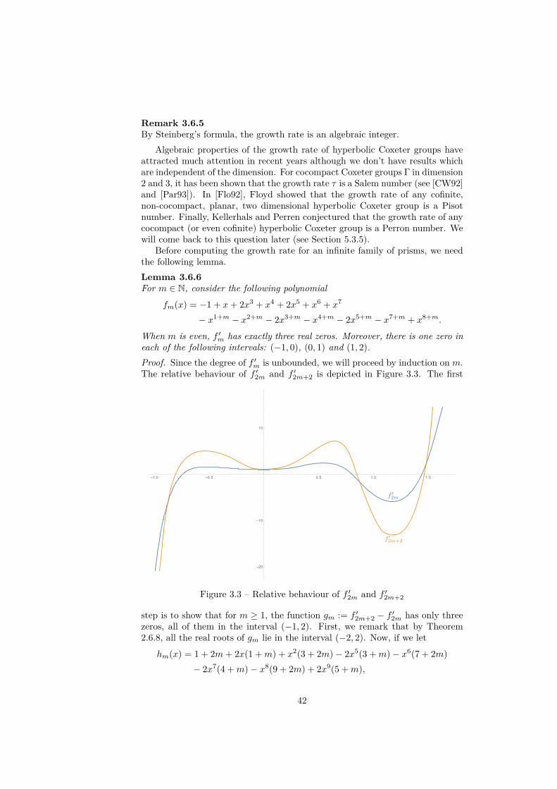
Remark 3.6.5By Steinberg’s formula, the growth rate is an algebraic integer.
Algebraic properties of the growth rate of hyperbolic Coxeter groups haveattracted much attention in recent years although we don’t have results whichare independent of the dimension. For cocompact Coxeter groups Γ in dimension2 and 3, it has been shown that the growth rate τ is a Salem number (see [CW92]and [Par93]). In [Flo92], Floyd showed that the growth rate of any cofinite,non-cocompact, planar, two dimensional hyperbolic Coxeter group is a Pisotnumber. Finally, Kellerhals and Perren conjectured that the growth rate of anycocompact (or even cofinite) hyperbolic Coxeter group is a Perron number. Wewill come back to this question later (see Section 5.3.5).
Before computing the growth rate for an infinite family of prisms, we needthe following lemma.Lemma 3.6.6For m ∈ N, consider the following polynomial
fm(x) = −1 + x+ 2x3 + x4 + 2x5 + x6 + x7
− x1+m − x2+m − 2x3+m − x4+m − 2x5+m − x7+m + x8+m.
When m is even, f ′m has exactly three real zeros. Moreover, there is one zero ineach of the following intervals: (−1, 0), (0, 1) and (1, 2).Proof. Since the degree of f ′m is unbounded, we will proceed by induction on m.The relative behaviour of f ′2m and f ′2m+2 is depicted in Figure 3.3. The first
Figure 3.3 – Relative behaviour of f ′2m and f ′2m+2
step is to show that for m ≥ 1, the function gm := f ′2m+2 − f ′2m has only threezeros, all of them in the interval (−1, 2). First, we remark that by Theorem2.6.8, all the real roots of gm lie in the interval (−2, 2). Now, if we let
hm(x) = 1 + 2m+ 2x(1 +m) + x2(3 + 2m)− 2x5(3 +m)− x6(7 + 2m)− 2x7(4 +m)− x8(9 + 2m) + 2x9(5 +m),
42

then we have gm(x) = x2m ·hm(x). Using Mathematica R© (see Section B.1.1), wecan compute a Sturm sequence (see Definition 2.6.3) p0 = hm, p1 = h′m, . . . , p9for each m. Moreover, since we have p0(−2) = −6647− 1338m, p0(−1) = −10,p0(0) = 1 + 2m, p0(1) = −14 and p0(2) = 1169 + 78m, we can use Sturm’stheorem (see Theorem 2.6.5) to count the zeros of hm(x) in the intervals (−1, 0),(0, 1) and (1, 2). We compute the signs of pi(αi) for αi = −2,−1, 0, 1, 2 and thenumber σ(αi) of sign changes:
αi 0 1 2 3 4 5 6 7 8 9 σ(αi)−2 − + − + + + − + + − 6−1 − + − + + + − − + − 60 + + − + + + − + + − 51 − − − + + − + + − − 42 + + + − − − + + − − 3
Since the number of zeros in (αi, αi+1) is given by σ(αi)−σ(αi+1), the first stepis done. We compute some values of f ′2m and f ′2m+2:
f ′2m+2(−1) = −2(11 + 5m) < f ′2m(−1) = −2(6 + 5m) < 0f ′2m(0) = 1f ′2m+2(1) = −2(1 + 7m) < f ′2m(1) = −2(7m− 6) < 0f ′2m+2(2) = 4m+1(26m+ 381) + 857 > f ′2m(2) = 4m(26m+ 355) + 857.
(3.3)
We found numerically that the roots of f ′2 are −0.740856, 0.880032 and 1.25209.Suppose now that f ′2m has the prescribed zeros (i.e. f ′2m has exactly three realzeros and there is exactly one in each of the three intervals (−1, 0), (0, 1) and(1, 2)). Since f ′2+2m has (at least) one change of sign in each of the interval(−1, 0), (0, 1) and (1, 2) (see equations (3.3)), then f ′2m+2 has at least the pre-scribed zeros. Now, since f ′2m+2 < f ′2m on (−∞,−1), f ′2m+2 has no zero onthis interval. To prove that f ′2m+2 has no zero on (2,∞) we use the fact thatf ′2m+2(x) > f ′2m(x) > 0 when x ∈ (2,∞). If f ′2m+2 has a second zero on (−1, 0),then so must have f ′2m (since gm has exactly one zero on (−1, 0)) and that isnot possible by the induction hypothesis. Hence, f ′2m+2 has exactly one zero on(−1, 0). We proceed in a similar way for the intervals (0, 1) and (1, 2).
Example 3.6.7We want to compute the growth series and the growth rate of the family of3-dimensional compact Coxeter prisms Γm whose graphs Gm are given in Fig-ure 3.4 (see [Kap74]). More precisely, we show that the sequence of growth
Figure 3.4 – A family of compact Coxeter prisms in H3
rates τm of Γm (which are Salem numbers since the groups are cocompact)converges to the Pisot number τ∞ ∼= 1.90648 which is the only real root of thepolynomial x7 − x6 − 2x4 − x3 − 2x2 − x− 1.
43
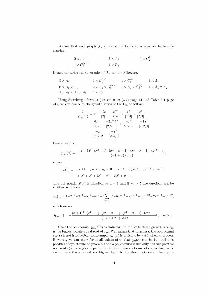
We see that each graph Gm contains the following irreducible finite sub-graphs:
5×A1 1×A2 1×G(4)2
1×G(m)2 1×B3
Hence, the spherical subgraphs of Gm are the following:
5×A1 1×G(m)2 1×G(4)
2 1×A2
6×A1 ×A1 2×A1 ×G(m)2 1×A1 ×G(4)
2 1×A1 ×A2
1×A1 ×A1 ×A1 1×B3
Using Steinberg’s formula (see equation (3.2) page 41 and Table 3.1 page41), we can compute the growth series of the Γm as follows:
1fΓm(x) = 1 + −5x
[2] + xm
[2,m] + x4
[2, 4] + x3
[2, 3]
+ 6x2
[2, 2] + −2xm+1
[2, 2,m] + −x5
[2, 2, 4] + −1x4
[2, 2, 3]
+ −x3
[2, 2, 2] + −x9
[2, 4, 6] .
Hence, we find
fΓm(x) = − (x+ 1)3 · (x2 + 1) · (x2 − x+ 1) · (x2 + x+ 1) · (xm − 1)(−1 + x) · q(x) ,
where
q(x) = −xm+1 − xm+2 − 2xm+3 − xm+4 − 2xm+5 − xm+7 + xm+8
+ x7 + x6 + 2x5 + x4 + 2x3 + x− 1.
The polynomial q(x) is divisible by x − 1 and if m > 5 the quotient can bewritten as follows
qm(x) = 1−2x3 −3x4 −5x5 −6x6 −7m∑i=7
xi−6xm+1 −5xm+2 −3xm+3 −2xm+4 +xm+7,
which means
fΓm(x) = − (x+ 1)3 · (x2 + 1) · (x2 − x+ 1) · (x2 + x+ 1) · (xm − 1)(−1 + x)2 · qm(x) , m ≥ 6.
Since the polynomial qm(x) is palindromic, it implies that the growth rate τmis the biggest positive real root of qm. We remark that in general the polynomialqm(x) is not irreducible: for example, qm(x) is divisible by x+1 when m is even.However, we can show for small values of m that qm(x) can be factored in aproduct of cyclotomic polynomials and a polynomial which only has two positivereal roots (since qm(x) is palindromic, these two roots are of course inverse ofeach other); the only real root bigger than 1 is thus the growth rate. The graphs
44
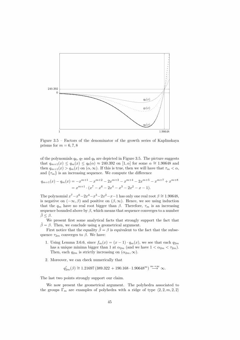
0240.392
1 1.90648
q6(x)
q7(x)
q8(x)
Figure 3.5 – Factors of the denominator of the growth series of Kaplinskayaprisms for m = 6, 7, 8
of the polynomials q6, q7 and q8 are depicted in Figure 3.5. The picture suggeststhat qm+1(x) ≤ qm(x) ≤ q6(α) ≈ 240.392 on [1, α] for some α ∼= 1.90648 andthen qm+1(x) > qm(x) on (α,∞). If this is true, then we will have that τm < α,and τm is an increasing sequence. We compute the difference
qm+1(x)− qm(x) = −xm+1 − xm+2 − 2xm+3 − xm+4 − 2xm+5 − xm+7 + xm+8
= xm+1 · (x7 − x6 − 2x4 − x3 − 2x2 − x− 1).
The polynomial x7−x6−2x4−x3−2x2−x−1 has only one real root β ∼= 1.90648,is negative on (−∞, β) and positive on (β,∞). Hence, we see using inductionthat the qm have no real root bigger than β. Therefore, τm is an increasingsequence bounded above by β, which means that sequence converges to a numberβ ≤ β.
We present first some analytical facts that strongly support the fact thatβ = β. Then, we conclude using a geometrical argument.
First notice that the equality β = β is equivalent to the fact that the subse-quence τ2m converges to β. We have:
1. Using Lemma 3.6.6, since fm(x) = (x − 1) · qm(x), we see that each q2mhas a unique minima bigger than 1 at α2m (and we have 1 < α2m < τ2m).Then, each q2m is strictly increasing on (α2m,∞).
2. Moreover, we can check numerically that
q′2m(β) ∼= 1.21697 (389.322 + 190.168 · 1.90648m) m→∞−→ ∞.
The last two points strongly support our claim.
We now present the geometrical argument. The polyhedra associated tothe groups Γm are examples of polyhedra with a ridge of type 〈2, 2,m, 2, 2〉
45
(see [Kol12, Section 3]) and they converge to the non-compact polyhedron P∞associated to the group Γ∞ given by the Coxeter symbol [∞, 3, 4,∞]. Now,[Kol12, Theorem 5] implies that the sequence τm converges to the growth rateτ∞ of Γ∞. This group has a growth series given by
fΓ∞(x) =(x+ 1)3 ·
(x2 + 1
)·(x2 − x+ 1
)·(x2 + x+ 1
)(x− 1) · (x7 + x6 + 2x5 + x4 + 2x3 + x− 1) .
Now, the polynomial x7 + x6 + 2x5 + x4 + 2x3 + x − 1 is irreducible and hasreciprocal polynomial x7−x6−2x4−x3−2x2−x−1 which implies τm
m→∞−→ τ∞,as required.
3.7 Euler characteristic, f-vector and volumeIn what follows, unless stated otherwise, Γ < IsomHn denotes a hyperbolicCoxeter group with finite set of natural generators S. Let P be its associatedfundamental convex polyhedron.
The next proposition gives the key tool which is used by CoxIter (see Chap-ter 5) to compute the orbifold Euler characteristic χ(Γ) of Hn/Γ.Proposition 3.7.1 ([KP11, (1.2) and (1.3)])Let (Γ, S) be an abstract Coxeter group and let F = T ⊂ S : ΓT is finite. Wehave
χ(Γ) =∑T∈F
(−1)|T |
fT (1) ,
where fT is the growth series of the group ΓT ≤ Γ generated by T (see Defini-tion 3.3.1).
In order to compute χ(Γ), we see by using the classification of finite Coxetergroups (see Figure 3.1) that it is sufficient to know the value fT (1) for allirreducible finite Coxeter groups. With the growth series (see Table 3.1), wefind the values given in Table 3.2.
Group fS(1)
Am (m+ 1)!
Bm 2m ·m!
Dm 2m−1 ·m!Gm 2mF4 1152
Group fS(1)
E6 51840E7 2903040E8 696729600H3 120H4 14400
Table 3.2 – Orders of finite Coxeter groups
The next result relates the Euler characteristic of a hyperbolic Coxeter groupΓ < IsomHn to its covolume when n is even.Proposition 3.7.2 ([KP11, (1.4)])When n is even, we have:
covolume(Γ) = (−1)n/2 · πn/2 · 2n · (n/2)!
n! · χ(Γ).
46
Remark 3.7.3When n is odd, we have χ(Γ) = 0.
We are also interested in the combinatorial properties of the Coxeter poly-hedron P associated to Γ.
Definition 3.7.4 (f -vector)The vector (f0, . . . , fn−1, 1) ∈ Zn+1, where fi is the number of faces of dimen-sion i of P , is called the f -vector of P (or f -vector of Γ)
To compute the f -vector, we will use the following results:
Theorem 3.7.5 ([Vin85, Theorem 3.1])Let G be the Coxeter diagram of Γ. There is a bijective correspondence betweenspherical subdiagrams of rank k of G and faces of codimension k of P .
Theorem 3.7.6 ([Vin85, Theorem 3.2])Let G be the Coxeter diagram of Γ. There is a bijective correspondence betweenparabolic subdiagrams of rank n− 1 of G and vertices at infinity of P .
As a test for the output of the program we also use the following classicalresult of Euler-Schläfli.
Proposition 3.7.7 ([Poi93])For a polyhedron in Xn, we have the following equality:
n−1∑i=0
(−1)i · fi = 1− (−1)n.
3.8 Compactness and finite volume criterionSince a polyhedron P is compact if and only if it is the convex hull of a finitenumber of vertices in Hn (also called ordinary vertices), we have the followingresult.
Proposition 3.8.1 ([Vin85, Proposition 4.2])The polyhedron P is compact if and only if the following conditions are satisfied:
• P contains at least one vertex (i.e. face of dimension 0) in Hn.
• For every vertex of P and every edge of P emanating from it there isprecisely one other vertex of P on that edge.
Since a polyhedron P is of finite volume if and only if it is the convex hullof a finite number of vertices in Hn, we have the following result.
Proposition 3.8.2 ([Vin85, Proposition 4.2])The polyhedron P has finite volume if and only if the following conditions aresatisfied:
• P contains at least one vertex (ordinary or at infinity).
• For every vertex (ordinary or at infinity) of P and every edge of P em-anating from it there is another vertex of P (ordinary or at infinity) onthat edge.
47

Using theorems 3.7.5 and 3.7.6 we deduce the following two criteria.
Proposition 3.8.3 (Cocompactness criterion in CoxIter)Let Γ < IsomHn be a Coxeter group and G be its Coxeter diagram. The groupΓ is cocompact if and only if the following conditions hold:
• G contains at least one spherical subdiagram of rank n.
• Each spherical subdiagram of rank n − 1 of G can be extended in exactlytwo ways to a spherical subdiagram of rank n of G.
Proposition 3.8.4 (Finite covolume criterion in CoxIter)Let Γ < IsomHn be a Coxeter group and G be its Coxeter diagram. The groupΓ has finite covolume if and only if the following conditions hold:
• G contains at least one spherical subdiagram of rank n or one parabolicsubdiagram of rank n− 1.
• Each spherical subdiagram of rank n − 1 of G can be extended in exactlytwo ways to one of the following type of subdiagrams of G:
– a spherical diagram of rank n;– a parabolic diagram of rank n− 1.
3.9 Arithmetic groups
3.9.1 DefinitionBefore we give the precise definition of an arithmetic group (of the simplesttype), we start with an example. Let fn(x) = −x0
2 + x12 + . . . + xn
2 be thestandard Lorentzian quadratic form and consider the cone C = x ∈ Rn+1 :fn(x) < 0. We denote by O(fn,Z) ⊂ GL(n + 1,R) the group of linear trans-formations of Rn+1 with coefficients in Z which preserve the quadratic formfn. The index two subgroup O+(fn,Z) consisting of elements of O(fn,Z) whichpreserve each of the two connected components of the cone C is the prototypeof an arithmetic group. Moreover, it is well known that this discrete grouphas finite covolume in O+(n, 1), which is related to hyperbolic isometries viaSO+(n, 1) = Isom+ Hn. Notice that the condition that the transformation hascoefficients in Z is equivalent to ask the preservation of the standard Z-latticein Rn+1. Now, let K be any totally real number field, OK its ring of integers,and let V be an (n+ 1)-dimensional vector space over K endowed with an ad-missible quadratic form f of signature (n, 1), that is: all conjugates fσ of f bythe non-trivial Galois embeddings σ : K −→ R are positive definite. The coneCf = x ∈ V ⊗R : f(x) < 0 has two connected components C±f and gives riseto the vector space model C+
f /R∗ of the hyperbolic n-space Hn (see Remarks3.2.2). We now let
O(f) =T ∈ GL(V ⊗ R) : f T (x) = f(x), ∀x ∈ V ⊗ R
.
Finally, for a full OK-lattice L in V , we consider the group
O(f, L) :=T ∈ O(f)K : T (C+
f ) = C+f , T (L) = L
.
It is a discrete subgroup of IsomHn of finite covolume (see [Bor62]).
48

Definition 3.9.1 (Arithmetic group (of the simplest type))A discrete group Γ < IsomHn is an arithmetic group of the simplest type ifthere exist K, f and L as above such that Γ is commensurable to O(f, L). Inthis setting, we say that Γ is defined over K and that f is the quadratic formassociated to Γ.
Remarks 3.9.2 1. In particular, an arithmetic group is cofinite.
2. If such a group is non-cocompact, then it must be defined over Q (see[Vin88, Chapter 6]).
3. If Γ is defined over Q, then it is non-cocompact if and only if the lattice isisotropic2 (see also [GP87, Section 2.3]). In particular, Γ is non-cocompactif n ≥ 4 (this follows from [Cas78, Chapter 4, Lemma 2.7] and the Hasse-Minkowski theorem).
4. There is a slightly more general definition of discrete arithmetic subgroupsof IsomHn. However, when a discrete subgroup of IsomHn is arith-metic and contains reflections, then it is of the simplest type (see [Vin67,Lemma 7]). In other words, an arithmetic hyperbolic Coxeter group isnot only commensurable to some O(f, L) but actually contained in someO(f, L). Since we focus in this work on Coxeter groups, we will refer toarithmetic of groups of the simplest type as arithmetic groups.
5. If OK is a PID, then the condition that the transformations T preservea lattice can be replaced by the condition that T has coefficients in OK .Indeed, in this setting, the lattice L is a free OK-module of rank n + 1with basis v1, . . . , vn+1. Now, the transformation X : ei 7−→ vi induces anisomorphism
O(f, L)∼=−→ O
(g,On+1
K
)φ 7−→ X−1 φ X,
where g := f X−1.
Reflective quadratic forms Consider, as above, an admissible quadraticform f of signature (n, 1) given by
f(x0, . . . , xn) =∑i,j
ai,j · xi xj , ai,j ∈ OK ,
with respect to some basis v0, . . . , vn, and consider L = spanOKv0, . . . , vn.As said above, the group O(f, L) is a discrete subgroup of IsomHn of finitecovolume. Moreover, we have the decomposition O(f, L) = Γ oH, where Γ isthe subgroup of O(f, L) generated by all the reflections in O(f, L) and H is asubgroup of the symmetry group of a cell of Γ.
Definition 3.9.3 (Reflective quadratic form)The quadratic form f is reflective if the group Γ in the decomposition O(f, L) =ΓoH has finite index in O(f, L). We note that it is equivalent to the fact thatP is finite sided and of finite covolume.
2In this setting, it means that there exists v ∈ V \ 0 such that f(v) = 0.
49

Example 3.9.4The Lorentzian quadratic form 〈−1, 1, . . . , 1〉 is reflective if and only if n ≤ 19(see [Vin72] and [KV78])
The next result allows to deal with the reflectivity of families of quadraticforms.
Proposition 3.9.5Let f be an admissible quadratic form of signature (n, 1) with n ≥ 3. If thequadratic form f ⊕ 〈1〉 is reflective, then so is f .
Proof. See [Bug90, Corollary 2].
We will come back to the question of reflectivity in the chapter 6), whichdedicated to Vinberg’s algorithm.
3.9.2 Criterion for arithmeticityIn [Vin67] and [Vin88], Vinberg presented a criterion to decide whether a dis-crete subgroup of IsomHn is arithmetic or not. In order to present the criterion,we need the following definition.
Definition 3.9.6 (Cycle in a matrix)Let A := (Ai,j) ∈ Mat(n;K) be a square matrix with coefficients in a field K. Acycle of length k, or k-cycle, in A is a product Ai1,i2 ·Ai2,i3 · . . . ·Aik−1,ik ·Aik,i1 .Such a cycle is denoted by A(i1,...,ik). If the ij are all distinct, the cycle is calledirreducible.
Theorem 3.9.7 (Arithmeticity criterion)Let Γ be a cofinite discrete subgroup of IsomHn generated by reflections and letG be its Gram matrix. Let K be the field generated by the entries of G andlet K ⊂ K be the field generated by the (irreducible) cycles in 2G. Then, Γ isarithmetic if and only if:
(i) K is a totally real number field;
(ii) for each Galois embedding σ : K −→ R which is not the identity on K,the matrix Gσ is positive semi-definite;
(iii) the cycles in 2G are algebraic integers in K.
In this case, the field of definition, or defining field, of Γ is K.
Proof. See [Vin88, Chapter 6, §3, Theorem 3.1].
Remark 3.9.8Observe that each cycle is a product of irreducible cycles. In particular, it issufficient to check condition (iii) only on irreducible cycles.
For a discrete subgroup of IsomHn generated by reflections, there is a weakerproperty called quasi-arithmeticity3. The precise definition of a quasi-arithmeticgroup, together with the proof of the next theorem, can be found in [Vin67].
3In fact, both arithmetic and quasi-arithmetic group can be defined in the more generalcontext of Lie groups and algebraic groups. More information can be found in [Vin67]
50
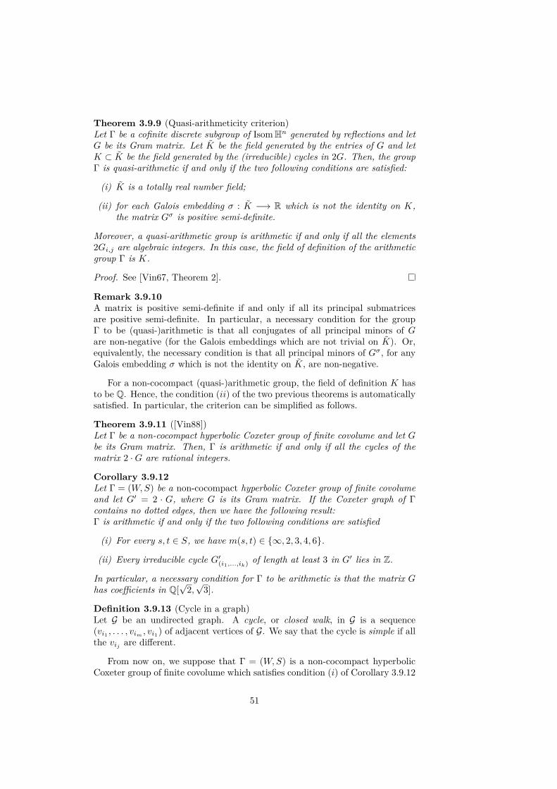
Theorem 3.9.9 (Quasi-arithmeticity criterion)Let Γ be a cofinite discrete subgroup of IsomHn generated by reflections and letG be its Gram matrix. Let K be the field generated by the entries of G and letK ⊂ K be the field generated by the (irreducible) cycles in 2G. Then, the groupΓ is quasi-arithmetic if and only if the two following conditions are satisfied:
(i) K is a totally real number field;
(ii) for each Galois embedding σ : K −→ R which is not the identity on K,the matrix Gσ is positive semi-definite.
Moreover, a quasi-arithmetic group is arithmetic if and only if all the elements2Gi,j are algebraic integers. In this case, the field of definition of the arithmeticgroup Γ is K.
Proof. See [Vin67, Theorem 2].
Remark 3.9.10A matrix is positive semi-definite if and only if all its principal submatricesare positive semi-definite. In particular, a necessary condition for the groupΓ to be (quasi-)arithmetic is that all conjugates of all principal minors of Gare non-negative (for the Galois embeddings which are not trivial on K). Or,equivalently, the necessary condition is that all principal minors of Gσ, for anyGalois embedding σ which is not the identity on K, are non-negative.
For a non-cocompact (quasi-)arithmetic group, the field of definition K hasto be Q. Hence, the condition (ii) of the two previous theorems is automaticallysatisfied. In particular, the criterion can be simplified as follows.
Theorem 3.9.11 ([Vin88])Let Γ be a non-cocompact hyperbolic Coxeter group of finite covolume and let Gbe its Gram matrix. Then, Γ is arithmetic if and only if all the cycles of thematrix 2 ·G are rational integers.
Corollary 3.9.12Let Γ = (W,S) be a non-cocompact hyperbolic Coxeter group of finite covolumeand let G′ = 2 · G, where G is its Gram matrix. If the Coxeter graph of Γcontains no dotted edges, then we have the following result:Γ is arithmetic if and only if the two following conditions are satisfied
(i) For every s, t ∈ S, we have m(s, t) ∈ ∞, 2, 3, 4, 6.
(ii) Every irreducible cycle G′(i1,...,ik) of length at least 3 in G′ lies in Z.
In particular, a necessary condition for Γ to be arithmetic is that the matrix Ghas coefficients in Q[
√2,√
3].
Definition 3.9.13 (Cycle in a graph)Let G be an undirected graph. A cycle, or closed walk, in G is a sequence(vi1 , . . . , vim , vi1) of adjacent vertices of G. We say that the cycle is simple if allthe vij are different.
From now on, we suppose that Γ = (W,S) is a non-cocompact hyperbolicCoxeter group of finite covolume which satisfies condition (i) of Corollary 3.9.12
51

and we let G′ = 2 · G. If s ∈ S is a leaf of the Coxeter graph (meaning thatm(s, t) = 2 for every t ∈ S \ s except for one vertex), then it is clear that scannot be a member of a non-zero irreducible cycle. Therefore, we can forgetthis vertex for the test. Also, any edge which is not part of a closed simplecycle can be dropped without changing the result of the test. Applying thisidea recursively until the graph does not change any more, in a process wewill call recursively deleting separating edges, lead to a simpler graph we cantest. For example, the two Coxeter graphs of Figure 3.6 are equivalent for thearithmeticity criterion.
Figure 3.6 – Two equivalent graphs for the arithmeticity criterion
Now, if G′(i1,...,ik) is an irreducible k-cycle, then it corresponds to a simplecycle in the Coxeter graph (see Definition 3.9.13) if and only if it is non-zero.Thus, it is sufficient to consider simple cycles in the Coxeter graph. This canbe summarized in the next proposition.
Proposition 3.9.14 (Arithmetic criterion in CoxIter ([Gug15]))Let Γ =
(W,S = s1, . . . , sd
)be a non-cocompact hyperbolic Coxeter group of
finite covolume and let G be its Coxeter graph. We suppose that G contains nodotted line. Then, Γ is arithmetic if and only if the two following conditions aresatisfied
1. For every s, t ∈ S, we have m(s, t) ∈ ∞, 2, 3, 4, 6.
2. For every simple cycle (si1 , . . . , sik , si1) in G, the product
2k ·k−1∏j=1
cos π
m(sij , sij+1) · cos π
m(sik , si1)
is an integer. Moreover, it is sufficient to test this condition in the graphobtained by recursively deleting separating edges.
Remark 3.9.15If the graph G contains dotted lines, we cannot decide the arithmeticity of thegroup only by looking at the weights m(s, t) in the graph. In order to extendProposition 3.9.14, we need to know the all values in the Gram matrix (Gij).If there is a dotted line between vertices i and j in G, a necessary condition forarithmeticity is that 4 ·G2
ij ∈ Z.
Remark 3.9.16For cocompact groups, the application of the criterion can be tricky. Examplescan be found in Section 4.4.1 which are based on Kaplinskaya’s 3-dimensionalprisms.
52

CHAPTER 4Commensurability
The aim of this chapter is to introduce the notion and to study the conceptof commensurability as well as to present a few methods which can be usedto decide the (non-)commensurability of two hyperbolic Coxeter groups. Thesetools are extensively used in a joint work with Matthieu Jacquemet and RuthKellerhals, where we classified a family of hyperbolic Coxeter pyramids withn+ 2 facets (see [GJK16]).
The first two sections are dedicated to the basic material and to an overviewof some of the methods used in our article. The details for the analytical, geo-metric and combinatorial methods can be found in [GJK16]. Then, a systematictreatment of the arithmetic case will be presented, which was my main contri-bution in our joint work. In particular, we explain in detail a method, firstdescribed by Maclachlan in [Mac11], to decide the commensurability for arith-metic groups of hyperbolic isometries. We also illustrate this method for newarithmetic cocompact hyperbolic Coxeter groups in IsomH4 and for the infinitefamilies of 3-dimensional prisms found by Kaplinskaya. Finally, we compute theinvariants for arithmetic hyperbolic Coxeter groups with underlying quadraticforms 〈−p, 1, . . . , 1〉 and 〈−1, p, 1, . . . , 1〉.
Before we start with the first definitions, let us make some general comments.First, since only very few families of hyperbolic Coxeter groups are entirelycharacterized, there are only very few families classified up to commensurability.Among them, we can cite:
1. Takeuchi gave a characterization of arithmetic Fuchsian groups in [Tak75](see also [Tak77a] for the particular case of triangle groups). He thenclassified arithmetic triangle groups up to commensurability in [Tak77b].
2. The cofinite hyperbolic Coxeter n-simplex groups (i.e. groups associatedto Coxeter polyhedra in Hn bounded by n+1 hyperplanes), which exist upto dimension 9, have been classified up to commensurability in [Joh+02].
3. The hyperbolic Coxeter groups in IsomHn, n ≥ 3, whose fundamentalpolyhedra are pyramids over a product of two simplices of positive dimen-sions, have been classified by Tumarkin in [Tum04]. These 200 pyramidCoxeter groups, which exists up to dimension 17, are classified up to com-mensurability in [GJK16] (see also theorems 4.0.1 and 4.0.2).
53
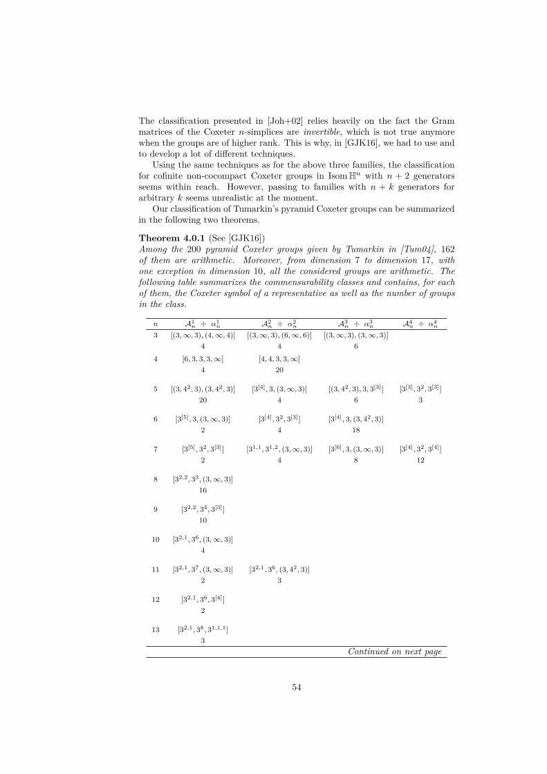
The classification presented in [Joh+02] relies heavily on the fact the Grammatrices of the Coxeter n-simplices are invertible, which is not true anymorewhen the groups are of higher rank. This is why, in [GJK16], we had to use andto develop a lot of different techniques.
Using the same techniques as for the above three families, the classificationfor cofinite non-cocompact Coxeter groups in IsomHn with n + 2 generatorsseems within reach. However, passing to families with n + k generators forarbitrary k seems unrealistic at the moment.
Our classification of Tumarkin’s pyramid Coxeter groups can be summarizedin the following two theorems.
Theorem 4.0.1 (See [GJK16])Among the 200 pyramid Coxeter groups given by Tumarkin in [Tum04], 162of them are arithmetic. Moreover, from dimension 7 to dimension 17, withone exception in dimension 10, all the considered groups are arithmetic. Thefollowing table summarizes the commensurability classes and contains, for eachof them, the Coxeter symbol of a representative as well as the number of groupsin the class.
n A1n ÷ α1
n A2n ÷ α2
n A3n ÷ α3
n A4n ÷ α4
n
3 [(3,∞, 3), (4,∞, 4)] [(3,∞, 3), (6,∞, 6)] [(3,∞, 3), (3,∞, 3)]4 4 6
4 [6, 3, 3, 3,∞] [4, 4, 3, 3,∞]4 20
5 [(3, 42, 3), (3, 42, 3)] [3[4], 3, (3,∞, 3)] [(3, 42, 3), 3, 3[3]] [3[3], 32, 3[3]]20 4 6 3
6 [3[5], 3, (3,∞, 3)] [3[4], 32, 3[3]] [3[4], 3, (3, 42, 3)]2 4 18
7 [3[5], 32, 3[3]] [31,1, 31,2, (3,∞, 3)] [3[6], 3, (3,∞, 3)] [3[4], 32, 3[4]]2 4 8 12
8 [32,2, 33, (3,∞, 3)]16
9 [32,2, 34, 3[3]]10
10 [32,1, 36, (3,∞, 3)]4
11 [32,1, 37, (3,∞, 3)] [32,1, 36, (3, 42, 3)]2 3
12 [32,1, 36, 3[4]]2
13 [32,1, 38, 31,1,1]3
Continued on next page
54

n A1n ÷ α1
n A2n ÷ α2
n A3n ÷ α3
n A4n ÷ α4
n
17 [32,1, 312, 31,2]1
Theorem 4.0.2 (See [GJK16])Among the 200 pyramid Coxeter groups given by Tumarkin in [Tum04], 38 ofthem are not arithmetic. The following table summarizes the commensurabilityclasses and contains, for each of them, the Coxeter symbol of a representative ofthe class. The header of the columns gives the number of elements in the class.
n |Nn| = 1 |Nn| = 2 |Nn| = 3 |Nn| = 4
3 [(3,∞, 4), (3,∞, 4)] [∞, 3, (3,∞, k)] [∞, 3, 5,∞]
k = 4, 5, 6
[∞, 3, (l,∞,m)]4 ≤ l < m ≤ 6
[∞, 4, (3,∞, 4)]
4 [6, 32, (k,∞, l)] [42, 3, (3,∞, 4)] [6, 32, 5,∞]
3 ≤ k < l ≤ 5
5 [4, 32,1, (3,∞, 4)]
6 [3, 4, 33, (3,∞, 4)]
10 [32,1, 36, (3,∞, 4)]
4.1 GeneralitiesDefinition 4.1.1 (Commensurable groups)Let Γ be a group and let Γ1 and Γ2 be two subgroups of Γ. We say that Γ1and Γ2 are commensurable if and only if the intersection Γ1∩Γ2 has finite indexboth in Γ1 and Γ2. They are said to be commensurable in the wide sense if Γ1 iscommensurable to a conjugate of Γ2. In this work, we will always use the termcommensurable to designate commensurable in the wide sense.
Definition 4.1.2 (Commensurable topological spaces)Two topological spaces X1 and X2 are said to be commensurable if they admithomeomorphic finite-sheeted coverings.
Proposition 4.1.3Two discrete subgroups Γ1,Γ2 of IsomHn are commensurable if and only if thetwo orbifolds Hn/Γ1 and Hn/Γ2 are commensurable.
The previous proposition implies in particular the following facts.
Proposition 4.1.4The ratio of the volumes of the associated polyhedra of two commensurable dis-crete hyperbolic Coxeter groups is a rational number. Moreover, for subgroupsof IsomHn, the following properties are stable by commensurability:
55

• being discrete;
• being cofinite;
• begin cocompact;
• being arithmetic.
The converse of the previous proposition is not true. In particular, thereexist incommensurable cofinite hyperbolic Coxeter groups of the same volume.
4.2 Different methods to test commensurabilityIn this section, we consider only cofinite hyperbolic Coxeter groups.
4.2.1 Subgroup relationsThe first trivial and most natural example of commensurability relation is theone of a finite index subgroup: every finite index subgroup is commensurablewith the bigger group. Some index two subgroups are easy to find by lookingat the Coxeter graph. It is the case, for example, when a vertex of the graphis connected to precisely one other vertex by a even weight. In this setting, thegroup contain an index two subgroup as shown in Figure 4.1 (see Proposition7.1.9, with I = s). Note that if ms,t =∞ in the situation depicted in Figure
Figure 4.1 – An index two subgroup
4.1, then ms′,t′ = ∞ as well (and the same holds when s and t are connectedby a dotted edge). More information and examples about index two subgroupsof Coxeter groups can be found in Chapter 7.
4.2.2 Invariant trace field and invariant quaternion alge-bra
Let Γ be a Kleinian group, that is, Γ is a cofinite discrete subgroup of Isom+ H3,which means that every element γ ∈ Γ is orientation preserving and has arepresentative γ ∈ SL(2;C). Let Γ(2) be the subgroup of Γ generated by squaresof elements of Γ.
Definition 4.2.1 (Invariant trace field)The field Q
(Tr γ : γ ∈ Γ(2)) generated by the traces of representatives of ele-
ments in SL(2;C) is called the invariant trace field and is denoted by K(Γ).
Proposition 4.2.2The invariant trace field K(Γ) is a finite extension of Q and is an invariant ofthe commensurability class of Γ.
56

Proof. See Theorems 3.1.2 and 3.3.4 of [MR03].
Let AΓ be the subring of Mat(2;C) generated by K(Γ) and by the represen-tatives γ ∈ SL(2;C) of the elements of Γ(2).
Proposition 4.2.3The ring AΓ is a quaternion algebra over K(Γ) and is an invariant of the com-mensurability class of Γ. Moreover, if Γ is non-cocompact, then the quaternionalgebra is trivial, that is AΓ ∼= Mat(2;K(Γ)).
Proof. See Theorem 3.2.1, Corollary 3.3.5 and Theorem 3.3.8 of [MR03].
Definition 4.2.4 (Invariant quaternion algebra)The quaternion algebra AΓ is called the invariant quaternion algebra.
Remarks 4.2.5 • In Section 4.3.2, we will see an effective way to computethe invariant trace field and the invariant quaternion algebra.
• For 3-dimensional cofinite arithmetic Coxeter groups, the pair (K(Γ), AΓ)is a complete invariant for the commensurability class.
4.2.3 CovolumesAs explained above, in order for two groups Γ1,Γ2 < IsomHn to be commen-surable, one must have covol Γ1
covol Γ2∈ Q. Of course, because of the Gauss-Bonnet
theorem, this condition is not interesting when the dimension n is even since thecovolume is a rational multiple of the volume of the n-sphere. More precisely,for n even and a cofinite Coxeter group Γ < IsomHn, we have
covolume(Γ) = (−1)n/2 · πn/2 · 2n · (n/2)!
n! · χ(Γ).
However, for n = 3 and n = 5 volume considerations can help to excludethe commensurability. As an example, consider the two arithmetic hyperbolicCoxeter pyramids depicted in Figure 4.2. These two groups have the sameinvariant trace field, K(Γ) = Q[
√2, i], and invariant quaternion algebra (which
is trivial, since the groups are non-cocompact, as indicated in Proposition 4.2.3).Moreover, one can show (see [GJK16]) that the volumes are given by
covol Γ1 = L(π
4
), covol Γ2 = 1
8 L(π
6
)+ L
(5π24
)−L
( π24
),
where L is the Lobachevsky function, defined by
L(x) = −∫ x
0log |2 sin t|dt, x ∈ R.
Then, one can show that the quotient covol Γ1covol Γ2
is irrational (see [GJK16, pp158-159]), which implies that Γ1 is not commensurable to Γ2.
57

Figure 4.2 – Three dimensional pyramids
4.3 Arithmetical aspectsIn [Mac11], Maclachlan described an effective way to decide the commensurabil-ity of two discrete arithmetic subgroups of IsomHn. The key point is that theclassification of arithmetic hyperbolic groups is equivalent to the classificationof their underlying quadratic forms up to similarity. In turn, the classification ofthese quadratic forms can be achieved using a complete set of invariants basedon quaternion algebras.
In this section, we present the result of Maclachlan and a few examples. Wefirst describe the general ideas behind the classification and then explain howto compute the complete set of invariants of an arithmetic hyperbolic Coxetergroups. We illustrate the method with examples in dimension 4 and 6 and thenconsider some infinite families described by Kaplinskaya. Other examples canbe found in [GJK16], where we classified 168 arithmetic pyramid groups.
4.3.1 ClassificationLet Γ1,Γ2 < IsomHn be two arithmetic Coxeter groups defined over the numberfields K1 and K2 respectively and let f1 and f2 be their underlying quadraticforms. A result of Gromov and Piatetski-Shapiro (see [GP87, Section 2.6])implies the following result:
Γ1 ∼ Γ2 ⇔ K1 = K2 and f1 ∼ f2,
where f1 ∼ f2 means that the two quadratic forms are similar (meaning thatthere exists c ∈ K1 = K2 such that c·f1 is isomorphic to f2). Therefore, decidingwhether Γ1 is commensurable to Γ2 can be done in two steps. First, we have tofind the defining fields and the underlying quadratic forms (see [Vin67, Part II,Theorem 2]). Secondly, we have to detect the similarity of the forms. The mainreferences for this section are [Mac11] and [Vin67].
Remark 4.3.1An immediate consequence of the result of Gromov and Piatetski-Shapiro is thefollowing: when n is odd, a necessary condition for Γ1 and Γ2 to be commen-surable is that K1 = K2 and that the quotient det f1/ det f2 is a square in K1.Indeed, if the forms are similar it means that there exists λ ∈ K∗1 such thatf1 ∼= λ · f2 and thus det f1 = λn+1 · det f2.
We will present the two points separately and illustrate them with an exam-ple: the goal is to decide whether the two subgroups Γ6
1,Γ62 < IsomH6 presented
in Figure 4.3 are commensurable or not. We first remark that these two groupsare arithmetic by virtue of Proposition 3.9.14:
58

• The Gram matrix of the first one has entries in Z[ 1
2].
• The graph of the second group contains only weights 3, 4 and 6 and nocycles.
The group Γ61 is the simplex group P 6 and has covolume 13
1360800 ·π3 (see Chap-
ter 5 or [Joh+99]). The group Γ62 is one of the pyramids given by Tumarkin in
[Tum04] and has covolume 13604800 ·π
3 (see Chapter 5); the ratio of their volumesis 4
9 . Since both groups are non-cocompact, the fields of definition are Q.
Figure 4.3 – Two arithmetic Coxeter subgroups of IsomH6
4.3.1.1 Finding the defining field and the underlying quadratic form
Let Γ < IsomHn be an arithmetic Coxeter group of rank d. We want to findthe defining field K and the underlying quadratic form f of Γ. We consider theassociated fundamental polyhedron P (Γ) and the outward-pointing normal unitvectors ei ∈ En,1 of the bounding hyperplanes Hi of P (Γ), which means thatP (Γ) =
⋂di=1H
−ei . Finally, we denote by G(Γ) = (ai,j) ∈ Mat(R; d) the Gram
matrix of Γ, meaning that ai,j = 〈ei, ej〉, for the Lorentzian product.Using Vinberg’s arithmeticity criterion (see Theorem 3.9.7), we can determinethe defining field K of Γ (recall that in this setting K is a totally real numberfield) by computing cycles in 2 ·G(Γ). Now, consider the K-subvector space Vof Rn+1 spanned by all the vectors
vi1,...,ik = 2k · a1,i1 · ai1,i2 · . . . · aik−1,ikeik , i1, . . . , ik ⊂ 1, . . . , d. (4.1)
The restriction of the Lorentzian form f0 to V is an admissible quadratic spaceof dimension n+ 1 over K. Moreover, Γ is commensurable to O(f, L), where Lis the lattice spanned over K by a basis v1, . . . , vn+1 of V and f is the quadraticform of signature (n, 1) defined by the symmetric matrix whose entries are theLorentzian products 〈vi, vj〉.
Hence, we have an explicit method to find the defining field K and theunderlying quadratic form f of an arithmetic hyperbolic Coxeter group Γ.Remark 4.3.2The task of finding the outward-pointing normal vectors of the polyhedron P (Γ)is difficult: one has to find the vectors e1, . . . , ed of En,1 such that 〈ei, ej〉 = ai,j .This basically is equivalent to solve a system of d(d+1)
2 quadratic equationswith d · (n + 1) unknowns. Assuming that e1 = (0, . . . , 0, 1) and that the firstvectors contain a lot of zeroes, we can guess the remaining vectors using softwaresuch as Mathematica R©. Another possibility is to compute sufficiently goodapproximations of the vectors ei using numerical methods and then use theLLL algorithm to find the exact components. This approach is described in[AMR09] for hyperbolic Coxeter groups in IsomH3. However, it seems thatextending this method to groups of higher ranks would be difficult.
59

The normal vectors of the polyhedra P (Γ61) and P (Γ6
2) associated to thegroups Γ6
1 and Γ62 (see Figure 4.3) are presented in Figure 4.4. We know that
the normal vectors of the simplex Γ61 are linearly independent and they all
appear on the right hand side of (4.1), up to a rescaling by a rational number.Therefore, we can take e1, . . . , e7 as a Q-basis of the space V . Hence, in thiscase, the underlying quadratic form is the form induced by the Gram matrix ofΓ6
1. In the case of the group Γ62, we find the following vectors:
e1, . . . , e8,√
2 · e2, . . . ,√
2 · e7,√
6 · e8.
We see that the vectors v1 := e1, v2 :=√
2 · e2, . . . , v7 :=√
2 · e7 are linearlyindependent over Q. We thus find the matrix of the quadratic form
(〈vi, vj〉
)i,j
=
1 0 −1 0 0 0 00 2 −1 0 0 0 0−1 −1 2 −1 0 0 00 0 −1 2 −1 0 00 0 0 −1 2 −1 00 0 0 0 −1 2 −10 0 0 0 0 −1 2
.
Finally, we consider the diagonal forms of these two quadratic forms (this canbe done using a software such as SageMath or by hand):
f61 = 〈1, 3, 6, 10, 15, 21,−21〉f6
2 = 〈1, 1, 2, 2, 2, 6,−1〉.
Here, q = 〈a1, . . . , am〉, with ai ∈ K, denotes the diagonal quadratic form withcoefficients a1, . . . , am, that is q is the quadratic form on Km defined by
q(x1, . . . , xm) =m∑i=1
ai · x2i , ∀(x1, . . . , xm) ∈ Km.
4.3.1.2 Constructing the invariants
Before we present the construction of the invariants, we briefly introduce itsingredients. The reader only interested in computations can skip this section.
For a quadratic space (V, f) we will consider the associated Clifford algebraCl(V, f) and its even subalgebra Cl0(V, f) (see Chapter 8 for more information).While Maclachlan requires that v2 = f(v) in Cl(V, q), we assume in Chapter 8that v2 = −f(v). This does not change the theory but simplifies our computa-tions.
Since the commensurability classes of arithmetic hyperbolic Coxeter groupsare determined by similarity classes of quadratic forms (see [GP87, §2.6]), wedefine, for a totally real number field1 K, the following map:
Θ : SimQF(K,n+ 1) −→ IsomAlg(K, 2n)[(V, f)
]7−→ Cl0(V, f),
1Recall that the field of definition of an arithmetic hyperbolic Coxeter group is a totallyreal number field.
60

e1 = (1, 0, 0, 0, 0, 0, 0)
e2 =(−
12,
16(6−√
6),
18(− 5 + 3
√6),
124(− 15
√2 + 22
√3),
124(− 9 + 11
√6),
12,
112(15− 11
√6))
e3 = (0,−1, 2, 2√
2, 2, 0,−4)
e4 =(
0, 0,−118,−
34√
2,−
58, 0,
54
)e5 = (0, 0, 0,−
√2, 0, 0, 1)
e6 =(
0, 0, 0, 0,−1,12,
12
)e7 = (0, 0, 0, 0, 0,−1, 0)
(a) Normal vectors of P (Γ61)
e1 = (1, 0, 0, 0, 0, 0, 0)
e2 =(
0,−1√
2,
1√
2, 0, 0, 0, 0
)e3 =
(−
1√
2,
1√
2, 0, 0, 0, 0, 0
)e4 =
(0,−
1√
2,−
1√
2,−√
32,−
12, 0,−1
)e5 =
(0, 0, 0,
√3
2,−
12, 0, 0
)e6 =
(0, 0, 0, 0, 1,
12,
12
)e7 = (0, 0, 0, 0, 0,−1, 0)
e8 =(
0, 0, 0,−12,−√
32,
√3
2,−√
32
)(b) Normal vectors of P (Γ6
2)
Figure 4.4 – Outward-pointing normal vectors of the Coxeter polyhedra associ-ated to the groups Γ6
1,Γ62 < IsomH6
where SimQF(K,n + 1) is the set of similarity classes of quadratic spaces overK of dimension n + 1 and IsomAlg(K, 2n) is the set of isomorphism classes ofalgebras overK of dimension 2n. If we restrict the map Θ to the quadratic formsf of signature (n, 1) whose conjugates fσ under non-trivial Galois embeddingsσ : K −→ R are positive definite, then we get an injective map (see [Mac11,Theorems 6.1 and 6.2]). Hence, we have to be able to decide whether theeven parts of the Clifford algebras (see Chapter 8) associated to the underlyingquadratic forms are isomorphic as algebras. Luckily for us, there is an efficientway to decide that using the Witt invariants and the Hasse invariants.
Definition 4.3.3 (Witt invariant)Let (V, f) be a quadratic space over a field K. The Witt invariant of (V, f),denoted by c(V, f), or only c(f), is the element of BrK defined as follows:
c(f) = c(V, f) :=[
Cl0(V, f)]
if dimV is odd,[Cl(V, f)
]if dimV is even.
Definition 4.3.4 (Hasse invariant)The Hasse invariant of a diagonal quadratic form 〈a1, . . . , an〉 over K is theelement of the Brauer group defined as follows:
s(〈a1, . . . , an〉) =⊗i<j
(ai, aj)K .
It can be shown (see [Lam05, Chapter V, Proposition 3.18]) that two isomorphicdiagonal quadratic forms have the same Hasse invariant. Therefore, we candefine the Hasse invariant of quadratic space (V, f) over K, or a quadratic formf over K, to be the Hasse invariant of any diagonalization of f . It will bedenoted by s(V, f) or just s(f).
61
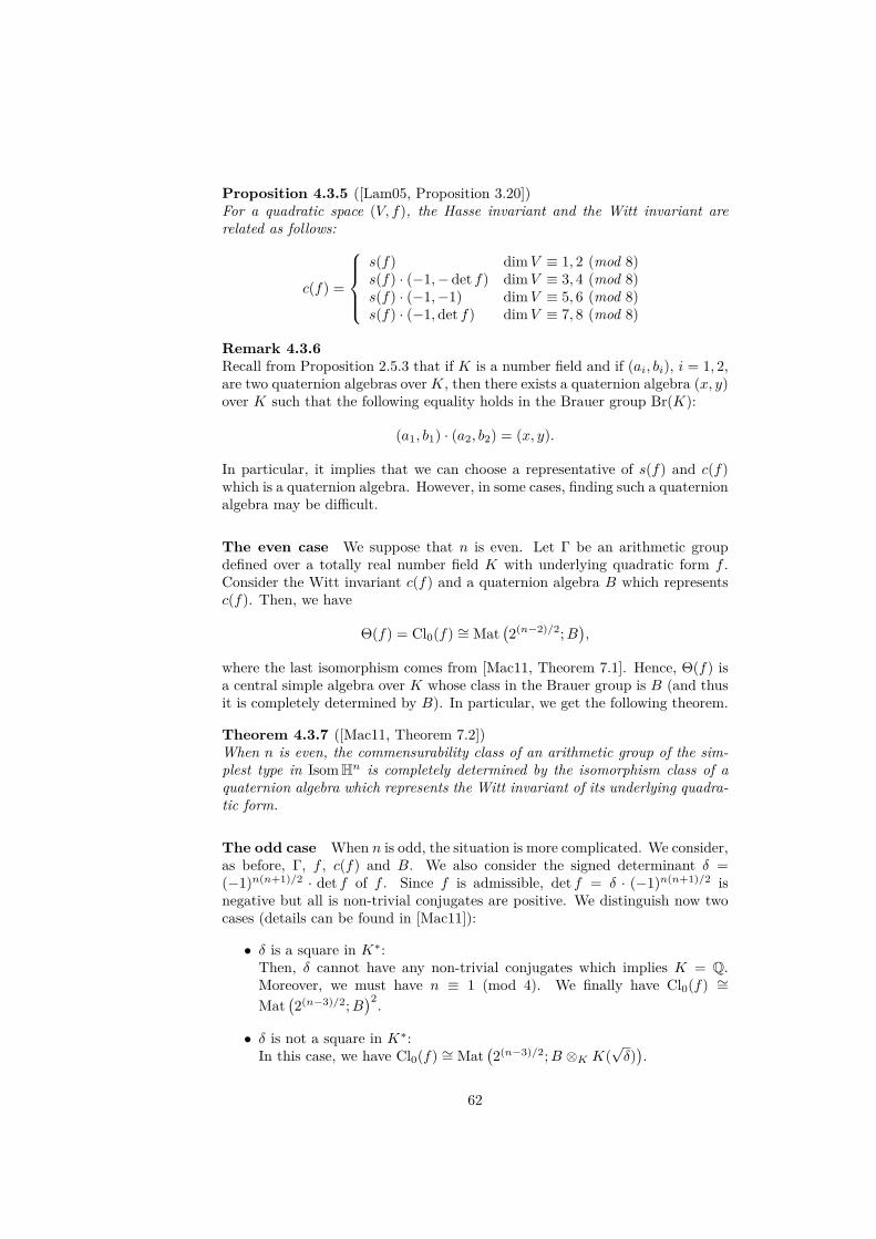
Proposition 4.3.5 ([Lam05, Proposition 3.20])For a quadratic space (V, f), the Hasse invariant and the Witt invariant arerelated as follows:
c(f) =
s(f) dimV ≡ 1, 2 (mod 8)s(f) · (−1,−det f) dimV ≡ 3, 4 (mod 8)s(f) · (−1,−1) dimV ≡ 5, 6 (mod 8)s(f) · (−1,det f) dimV ≡ 7, 8 (mod 8)
Remark 4.3.6Recall from Proposition 2.5.3 that if K is a number field and if (ai, bi), i = 1, 2,are two quaternion algebras overK, then there exists a quaternion algebra (x, y)over K such that the following equality holds in the Brauer group Br(K):
(a1, b1) · (a2, b2) = (x, y).
In particular, it implies that we can choose a representative of s(f) and c(f)which is a quaternion algebra. However, in some cases, finding such a quaternionalgebra may be difficult.
The even case We suppose that n is even. Let Γ be an arithmetic groupdefined over a totally real number field K with underlying quadratic form f .Consider the Witt invariant c(f) and a quaternion algebra B which representsc(f). Then, we have
Θ(f) = Cl0(f) ∼= Mat(2(n−2)/2;B
),
where the last isomorphism comes from [Mac11, Theorem 7.1]. Hence, Θ(f) isa central simple algebra over K whose class in the Brauer group is B (and thusit is completely determined by B). In particular, we get the following theorem.
Theorem 4.3.7 ([Mac11, Theorem 7.2])When n is even, the commensurability class of an arithmetic group of the sim-plest type in IsomHn is completely determined by the isomorphism class of aquaternion algebra which represents the Witt invariant of its underlying quadra-tic form.
The odd case When n is odd, the situation is more complicated. We consider,as before, Γ, f , c(f) and B. We also consider the signed determinant δ =(−1)n(n+1)/2 · det f of f . Since f is admissible, det f = δ · (−1)n(n+1)/2 isnegative but all is non-trivial conjugates are positive. We distinguish now twocases (details can be found in [Mac11]):
• δ is a square in K∗:Then, δ cannot have any non-trivial conjugates which implies K = Q.Moreover, we must have n ≡ 1 (mod 4). We finally have Cl0(f) ∼=Mat
(2(n−3)/2;B
)2.• δ is not a square in K∗:In this case, we have Cl0(f) ∼= Mat
(2(n−3)/2;B ⊗K K(
√δ)).
62
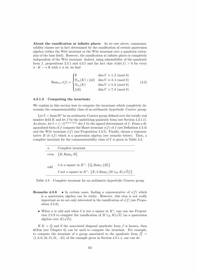
About the ramification at infinite places As we saw above, commensu-rability classes are in fact determined by the ramification of certain quaternionalgebra (either the Witt invariant or the Witt invariant over a quadratic exten-sion of the base field). However, the ramification at infinite places is completelyindependent of the Witt invariant. Indeed, using admissibility of the quadraticform f , propositions 2.5.1 and 4.3.5 and the fact that σ(det f) > 0 for everyσ : K −→ R with σ 6= id, we find
Ram∞ c(f) =
∅ dimV ≡ 1, 2 (mod 8)Ω∞(K) \ id dimV ≡ 3, 4 (mod 8)Ω∞(K) dimV ≡ 5, 6 (mod 8)id dimV ≡ 7, 8 (mod 8)
(4.2)
4.3.1.3 Computing the invariants
We explain in this section how to compute the invariants which completely de-termine the commensurability class of an arithmetic hyperbolic Coxeter group.
Let Γ < IsomHn be an arithmetic Coxeter group defined over the totally realnumber field K and let f be the underlying quadratic form (see Section 4.3.1.1).As above, let δ = (−1)n(n+1)/2 ·det f be the signed determinant of f . From a di-agonalized form of f compute the Hasse invariant s(f) of f (see Definition 4.3.4)and the Witt invariant c(f) (see Proposition 4.3.5). Finally, choose a represen-tative B of c(f) which is a quaternion algebra (see remarks below). Then, acomplete invariant for the commensurability class of Γ is given in Table 4.3.
n Complete invariant
evenK,Ramf B
odd δ is a square in K∗:
Q,Ramf
(B)
δ not a square in K∗:K, δ,Ramf
(B ⊗K K(
√δ))
Table 4.3 – Complete invariant for an arithmetic hyperbolic Coxeter group
Remarks 4.3.8 • In certain cases, finding a representative of c(f) whichis a quaternion algebra can be tricky. However, this step is not reallyimportant as we are only interested in the ramification of c(f) (see Propo-sition 2.5.8).
• When n is odd and when δ is not a square in K∗, one can use Proposi-tion 2.5.9 to compute the ramification of B ⊗K K(
√δ) (as a quaternion
algebra over K(√δ)).
If K = Q and if the associated diagonal quadratic form f is known, thenAlVin (see Chapter 6) can be used to compute the invariant. For example,to compute the invariant of a group associated to the quadratic form f6
1 =〈1, 3, 6, 10, 15, 21,−21〉 of the example given in Section 4.3.1.1, one can do
63

./ alvin -maxv 1 -iqf -qf 1 ,3 ,6 ,10 ,15 ,21 , -21
The "-maxv 1" option indicates not to compute normal vectors and the "-iqf"parameter (for invariant of the quadratic form) asks the program to display theinvariant. Then, the output is the following:Commensurability invariant :
Q, infinity ,3
Therefore, the commensurability invariant of the group Γ61 is
Q, ∞, 3
.
4.3.1.4 Finishing the analysis for the examples in dimension 6
We come back to our two examples in dimension 6 defined over Q and withquadratic forms
f61 = 〈1, 3, 6, 10, 15, 21,−21〉f6
2 = 〈1, 1, 2, 2, 2, 6,−1〉.
We first compute the Hasse invariants s(f6i ) for i = 1, 2. Recall that for a
diagonal quadratic form f = 〈a1, . . . , am〉, we have s(f) =⊗
i<j(ai, aj) ∈ BrK.Using the properties of Proposition 2.5.2, we compute:
s(f61 ) = (3, 6) · (3, 10) · (3, 15) ·
(3,−1)︷ ︸︸ ︷(3, 21) · (3,−21)
· (6, 10) · (6, 15) · (6,−1)· (10, 15) · (10,−1)· (15,−1)
= (5,−1).
Similarly, we find s(f62 ) = 1. Using Proposition 4.3.5 we find c(f6
1 ) = (5,−1) ·(−1,−3) = (−1,−15) and c(f6
2 ) = 1 ·(−1,−3). By Proposition 2.5.10 we obtainthe following ramification sets:
Ram(−1,−3) = 3,∞, Ram(−1, 5) = ∅.
Finally, using Proposition 2.5.8 we get Ramf c(f61 ) = 3,∞ = Ramf c(f6
2 ),which implies that the groups Γ6
1 and Γ62 are commensurable.
4.3.1.5 New cocompact examples worked out in detail
We study the commensurability of three cocompact arithmetic Coxeter sub-groups Γ4
i , i = 1, 2, 3, of IsomH4. These groups correspond to maximal sub-groups generated by reflections in the groups of units O(fi,OK5) of three (reflec-tive) quadratic forms fi with base field K = Q[
√5] and they were found using
Vinberg’s algorithm (see Chapter 6). For simplicity, we write Θ = 1+√
52 for the
generator of the ring of integers of OK = Z[Θ]. The first group is the simplexgroup [5, 3, 3, 4] and is associated to the quadratic form f1 = 〈−Θ, 1, 1, 1, 1〉(see [Bug84]) while the last two correspond to new Coxeter polyhedra P (Γ4
i ),i = 2, 3, I discovered (see Section 6.8.3) and are associated to the quadraticforms f2 = 〈−Θ, 1, 1, 1, 2 + Θ〉 and f3 = 〈−Θ, 1, 1, 2 + Θ, 2 + Θ〉 respectively.The Coxeter graphs of the first two groups are presented in Figure 4.5.
64
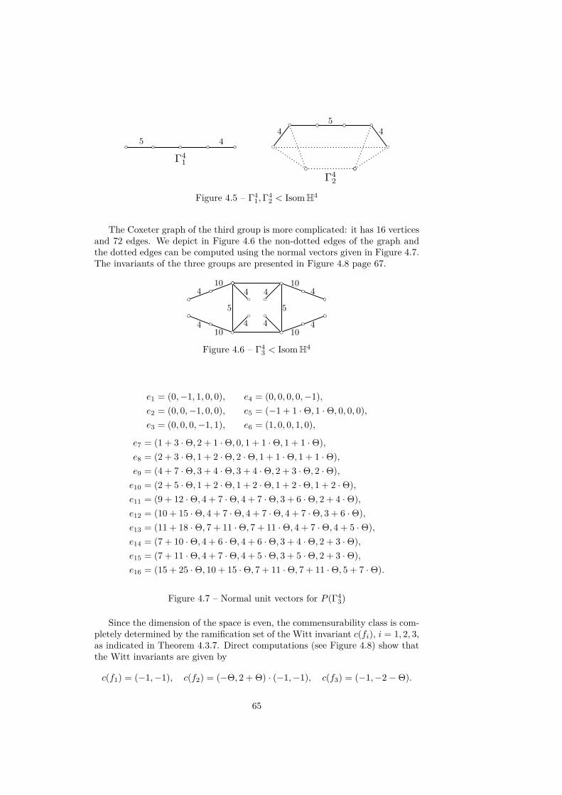
Figure 4.5 – Γ41,Γ4
2 < IsomH4
The Coxeter graph of the third group is more complicated: it has 16 verticesand 72 edges. We depict in Figure 4.6 the non-dotted edges of the graph andthe dotted edges can be computed using the normal vectors given in Figure 4.7.The invariants of the three groups are presented in Figure 4.8 page 67.
Figure 4.6 – Γ43 < IsomH4
e1 = (0,−1, 1, 0, 0), e4 = (0, 0, 0, 0,−1),e2 = (0, 0,−1, 0, 0), e5 = (−1 + 1 ·Θ, 1 ·Θ, 0, 0, 0),e3 = (0, 0, 0,−1, 1), e6 = (1, 0, 0, 1, 0),
e7 = (1 + 3 ·Θ, 2 + 1 ·Θ, 0, 1 + 1 ·Θ, 1 + 1 ·Θ),e8 = (2 + 3 ·Θ, 1 + 2 ·Θ, 2 ·Θ, 1 + 1 ·Θ, 1 + 1 ·Θ),e9 = (4 + 7 ·Θ, 3 + 4 ·Θ, 3 + 4 ·Θ, 2 + 3 ·Θ, 2 ·Θ),e10 = (2 + 5 ·Θ, 1 + 2 ·Θ, 1 + 2 ·Θ, 1 + 2 ·Θ, 1 + 2 ·Θ),e11 = (9 + 12 ·Θ, 4 + 7 ·Θ, 4 + 7 ·Θ, 3 + 6 ·Θ, 2 + 4 ·Θ),e12 = (10 + 15 ·Θ, 4 + 7 ·Θ, 4 + 7 ·Θ, 4 + 7 ·Θ, 3 + 6 ·Θ),e13 = (11 + 18 ·Θ, 7 + 11 ·Θ, 7 + 11 ·Θ, 4 + 7 ·Θ, 4 + 5 ·Θ),e14 = (7 + 10 ·Θ, 4 + 6 ·Θ, 4 + 6 ·Θ, 3 + 4 ·Θ, 2 + 3 ·Θ),e15 = (7 + 11 ·Θ, 4 + 7 ·Θ, 4 + 5 ·Θ, 3 + 5 ·Θ, 2 + 3 ·Θ),e16 = (15 + 25 ·Θ, 10 + 15 ·Θ, 7 + 11 ·Θ, 7 + 11 ·Θ, 5 + 7 ·Θ).
Figure 4.7 – Normal unit vectors for P (Γ43)
Since the dimension of the space is even, the commensurability class is com-pletely determined by the ramification set of the Witt invariant c(fi), i = 1, 2, 3,as indicated in Theorem 4.3.7. Direct computations (see Figure 4.8) show thatthe Witt invariants are given by
c(f1) = (−1,−1), c(f2) = (−Θ, 2 + Θ) · (−1,−1), c(f3) = (−1,−2−Θ).
65

Therefore, in order to decide about the commensurability of our groups, wehave to compute the finite ramification of the quaternion algebras (−1,−1)K ,(−Θ, 2 + Θ)K and (−1, 2 + Θ)K .
Using Proposition 2.5.9 we see that Ramf (−1,−1) = ∅. Since NK/Q(−Θ) =−1, then −Θ is invertible, while NK/Q(2 + Θ) = 5 implies that 2 + Θ is aprime element of OK lying over 5. For a quaternion algebra (a, b)K , a necessarycondition for a prime ideal P ⊂ OK to belong to the ramification set is that P |〈2ab〉 = (2ab)OK . In our case, since 2 remains prime in OK , the only candidatesare 2 and
√5. Moreover, since the ramification set has even cardinality (see
Theorem 2.5.5) and since |Ram∞Bi| = 2 (see equation (4.2) page 63), theneither Ramf Bi = ∅ or Ramf Bi = 2,
√5. To compute the ramification, we
will use the following theorem.
Theorem 4.3.9 ([AMR09, Theorem 16])Let K be a number field. Let P be a prime ideal of OK and let a, b ∈ OK be suchthat the valuations of these elements satisfy ηP(a), ηP(b) ∈ 0, 1. We define aninteger m as follows:
• if P | 〈2〉, m = 2ηP(2) + 3;
• if P - 〈2〉, then m = 1 if ηP(a) = ηP(b) = 0 and m = 3 otherwise.
We also let S be a finite set of representatives for the ring OK/Pm.Then, P /∈ Ramf (a, b)K , i.e. (a, b) splits at P, if and only if there exists a triple(X,Y, Z) ∈ S3 such that the two following conditions are satisfied:
• aX2 + bY 2 − Z2 = 0 or m ≤ ηP(aX2 + bY 2 − Z2);
• ηP(X) = 0 or ηP(Y ) = 0 or ηP(Z) = 0.
Remark 4.3.10Since (ac2, b) ∼= (a, b), the condition ηP(a), ηP(b) ∈ 0, 1 is not a restriction.
We start with the group Γ42. We take P = 〈
√5〉 and a = −Θ, b = 2 + Θ,
which gives ηP(a) = 0 and ηP(b) = 1 and thus m = 3. The quotient OK/P3
has 125 elements which can be described as follows (see [EIR11, Theorem 1]):
OK/P3 =
(x+ y√
5)P3 : 0 ≤ x < 25, 0 ≤ y < 5.
Using a computer, we can check by means of Theorem 4.3.9 that√
5 belongsto Ramf (−Θ, 2 + Θ) and thus
√5 ∈ Ramf B2. Therefore, we have Ramf B2 =
2,√
5. On the other hand, since the equation (2 + Θ)X2 − Y 2 − Z2 = 0is satisfied with X = Y = −1 + Θ and Z = 1 (and thus ηP(X) = ηP(Y ) =ηP(Z) = 0), then
√5 6∈ Ramf (−1, 2 + Θ) which implies that Ramf B3 = ∅.
Hence, the simplex group Γ41 is commensurable to the group Γ4
3 but not to Γ42.
4.3.2 Case n = 3 (arithmetic and non-arithmetic)When n = 3, we have two interesting features concerning (in-)commensurablegroups in IsomH3:
• the computation of the invariants is easier;
• some of the results are true even when the groups are not arithmetic.
66

invariant Γ41 Γ4
2 Γ43
fi 〈−Θ, 1, 1, 1, 1〉 〈−Θ, 1, 1, 1, 2 + Θ〉 〈−Θ, 1, 1, 2 + Θ, 2 + Θ〉
f -vector (5, 10, 10, 5, 1) (14, 28, 22, 8, 1) (48, 96, 64, 16, 1)
covol. 1721600 · π
2 160 · π
2 221900 · π
2
s(fi) 1 (−Θ, 2 + Θ) (−1, 2 + Θ)
c(fi) (−1,−1) (−Θ, 2 + Θ) · (−1,−1) (−1,−2−Θ)
Ramf Bi ∅ 2,√
5 ∅
Figure 4.8 – Invariants of the three 4-dimensional cocompact groups Γ4i
A standard reference for the three dimensional case is [MR03]. Let Γ < IsomH3
be a cofinite Coxeter group (not necessarily arithmetic) of rank d. As above,we denote by G(Γ) = (ai,j) the Gram matrix of Γ and by ei the normal vectorsunit of the bounding hyperplanes Hei of the fundamental polyhedron P (Γ) ofΓ. We let K be the field generated by the cycles in G(Γ):
K = Q(ai1,i2 · . . . · aik−1,ik · aik,i1 : ij ∈ 1, . . . , d
).
We also consider the K-vector space M(Γ) spanned by the vectors
a1,i1 · ai1,i2 · . . . · aik−1,ik · eik , ij ∈ 1, . . . , d.
This space, endowed with the restriction of the Lorentzian form, is a quadraticspace of signature (3, 1). If we let δ be the determinant of this quadratic spacewe then have the following results.
Proposition 4.3.11 ([MR98, Theorem 3.1])The field K(
√δ) is equal to the invariant trace field.
Let 〈−a1, a2, a3, a4〉, ai > 0, be a diagonal form of the quadratic form corre-sponding to M(P ).
Proposition 4.3.12 ([MR98, Theorem 3.1])The invariant quaternion algebra AΓ is given by (a1 · a2, a1 · a3)K(Γ).
Theorem 4.3.13 ([MR03, Theorem 3.3.8])If Γ is non-cocompact, then AΓ = 1.
Remark 4.3.14If Γ is arithmetic, then the invariant trace field and the invariant quaternionalgebra correspond to what we get using the Witt invariant (and thus form acomplete set of invariants). Indeed, since we are only interested in the similarityclass of the quadratic form, we can suppose that it can be written in the form〈1, b, c,−d〉, with b, c, d > 0. We then let δ = −bcd be the determinant of theform which gives
〈1, b, c, d〉 ∼= 〈1,−δcd,−δbd, δbc〉 = 〈1,−δc,−δd, δcd〉,
with c := cd, d := bd. Then, a direct computation shows that the Witt invariantof this last quadratic form is (c, d) = (cd, bd).
67

4.4 Examples
4.4.1 Kaplinskaya’s 3-dimensional familiesIn this section, we present the computations of the commensurability invariantsfor some families of Coxeter prisms in H3 given by Kaplinskaya in [Kap74]. Thesummary of the invariants for these families can be found in the appendicesA.1.1 and A.1.2. The infinite families of Kaplinskaya are of special interest sincethey are the among the very few known infinite families of hyperbolic Coxetergroups not arising as sequences of doublings (see Chapter 7 for examples of suchsequences).
Example 4.4.1We continue to study the family of 3-dimensional cocompact groups Γm shown inFigure 4.9 (see Example 3.6.7 for the growth series and the growth rates of thesegroups). Our aim is to decide which groups of the family are (quasi-)arithmeticand to compute the invariant trace field and the invariant quaternion algebra.The Gram matrix of such a group is given by Gm and has the following form
Figure 4.9 – A family of 3-dimensional compact Coxeter prisms
Gm =
1 −√
3 cos( 2πm )+1
2√
cos( 2πm )
0 0 0
−√
3 cos( 2πm )+1
2√
cos( 2πm )
1 − 12 0 0
0 − 12 1 − 1√
2 00 0 − 1√
2 1 − cos(πm
)0 0 0 − cos
(πm
)1
.
In order for Γm to be (quasi-)arithmetic, it is necessary that all the entriesof Gm are totally real algebraic numbers. Since cos π
m is always a totally realalgebraic number we will see for which value of m there is at least one conjugateof αm := 3 cos( 2π
m )+1cos( 2π
m ) which is negative. Thus, if there exists an integer k < m
which is coprime with m and such that the image 3 cos( 2kπm )+1
cos( 2kπm ) of αm by the
Galois automorphism corresponding to k is negative, then Γm is not quasi-arithmetic. This happens when k lies between 1
4m and arccos(− 1
3)· 1
2π ·m ∼=0.304087 · m. Therefore, we see using Theorem 2.3.1 with ε = 1
5 that Γmis not quasi-arithmetic if m ≥ 100. Direct computations show that the onlypossibilities are m ∈ 5, 6, 8, 9, 12, 13, 14, 16, 20, 21, 22, 28, 30, 36,54. Since the minimal polynomial of
(2 ·Gm
)1,2 = −√αm is not monic when
m ∈ 12, 20, 28, 36, then Γm cannot be arithmetic for these values.Now, the field K generated by the cycles in 2Gm is Q
[cos 2π
m
]and the field
K generated by the entries of Gm is Q[cos π
m ,√αm,√
2]. For m ∈ 5, 6, 8, 9,
12, 13, 14, 16, 20, 21, 22, 28, 30, 36, 54, the group Γm will be quasi-arithmetic if
68
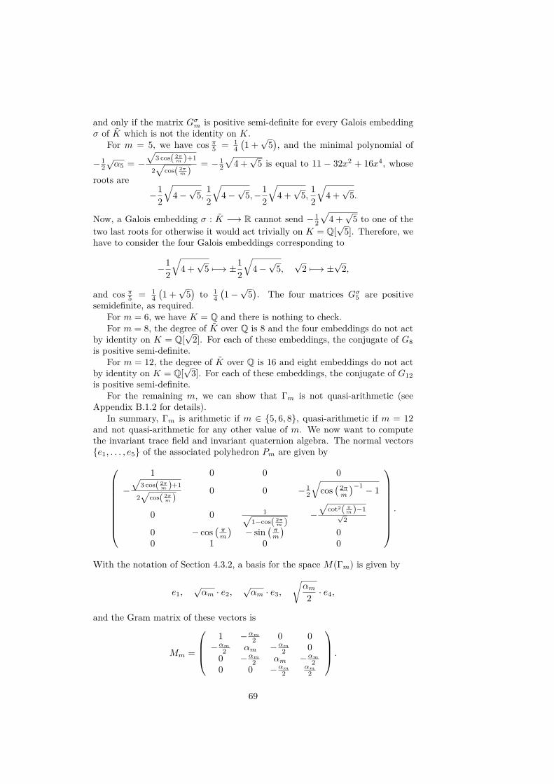
and only if the matrix Gσm is positive semi-definite for every Galois embeddingσ of K which is not the identity on K.
For m = 5, we have cos π5 = 14(1 +√
5), and the minimal polynomial of
− 12√α5 = −
√3 cos( 2π
m )+1
2√
cos( 2πm )
= − 12
√4 +√
5 is equal to 11 − 32x2 + 16x4, whose
roots are−1
2
√4−√
5, 12
√4−√
5,−12
√4 +√
5, 12
√4 +√
5.
Now, a Galois embedding σ : K −→ R cannot send − 12
√4 +√
5 to one of thetwo last roots for otherwise it would act trivially on K = Q[
√5]. Therefore, we
have to consider the four Galois embeddings corresponding to
−12
√4 +√
5 7−→ ±12
√4−√
5,√
2 7−→ ±√
2,
and cos π5 = 14(1 +√
5)to 1
4(1−√
5). The four matrices Gσ5 are positive
semidefinite, as required.For m = 6, we have K = Q and there is nothing to check.For m = 8, the degree of K over Q is 8 and the four embeddings do not act
by identity on K = Q[√
2]. For each of these embeddings, the conjugate of G8is positive semi-definite.
For m = 12, the degree of K over Q is 16 and eight embeddings do not actby identity on K = Q[
√3]. For each of these embeddings, the conjugate of G12
is positive semi-definite.For the remaining m, we can show that Γm is not quasi-arithmetic (see
Appendix B.1.2 for details).In summary, Γm is arithmetic if m ∈ 5, 6, 8, quasi-arithmetic if m = 12
and not quasi-arithmetic for any other value of m. We now want to computethe invariant trace field and invariant quaternion algebra. The normal vectorse1, . . . , e5 of the associated polyhedron Pm are given by
1 0 0 0
−√
3 cos( 2πm )+1
2√
cos( 2πm )
0 0 − 12
√cos( 2πm
)−1 − 1
0 0 1√1−cos( 2π
m )−√
cot2( πm )−1√
2
0 − cos(πm
)− sin
(πm
)0
0 1 0 0
.
With the notation of Section 4.3.2, a basis for the space M(Γm) is given by
e1,√αm · e2,
√αm · e3,
√αm2 · e4,
and the Gram matrix of these vectors is
Mm =
1 −αm2 0 0−αm2 αm −αm2 0
0 −αm2 αm −αm20 0 −αm2
αm2
.
69
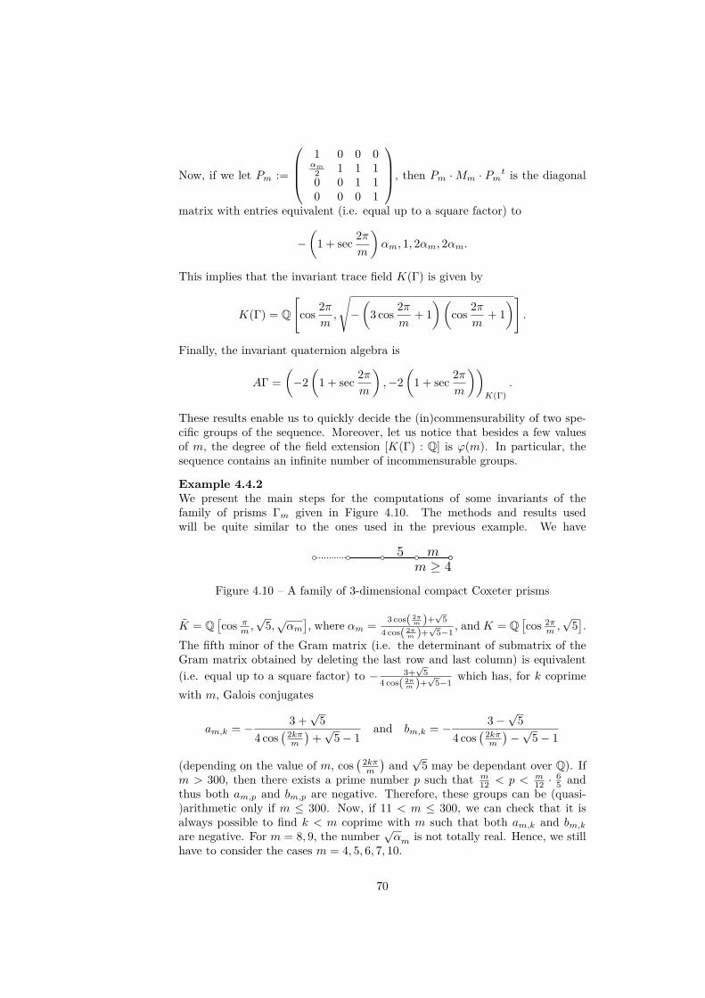
Now, if we let Pm :=
1 0 0 0αm2 1 1 10 0 1 10 0 0 1
, then Pm ·Mm · Pmt is the diagonal
matrix with entries equivalent (i.e. equal up to a square factor) to
−(
1 + sec 2πm
)αm, 1, 2αm, 2αm.
This implies that the invariant trace field K(Γ) is given by
K(Γ) = Q
[cos 2π
m,
√−(
3 cos 2πm
+ 1)(
cos 2πm
+ 1)]
.
Finally, the invariant quaternion algebra is
AΓ =(−2(
1 + sec 2πm
),−2
(1 + sec 2π
m
))K(Γ)
.
These results enable us to quickly decide the (in)commensurability of two spe-cific groups of the sequence. Moreover, let us notice that besides a few valuesof m, the degree of the field extension [K(Γ) : Q] is ϕ(m). In particular, thesequence contains an infinite number of incommensurable groups.
Example 4.4.2We present the main steps for the computations of some invariants of thefamily of prisms Γm given in Figure 4.10. The methods and results usedwill be quite similar to the ones used in the previous example. We have
Figure 4.10 – A family of 3-dimensional compact Coxeter prisms
K = Q[cos π
m ,√
5,√αm], where αm = 3 cos( 2π
m )+√
54 cos( 2π
m )+√
5−1, andK = Q
[cos 2π
m ,√
5].
The fifth minor of the Gram matrix (i.e. the determinant of submatrix of theGram matrix obtained by deleting the last row and last column) is equivalent(i.e. equal up to a square factor) to − 3+
√5
4 cos( 2πm )+
√5−1
which has, for k coprimewith m, Galois conjugates
am,k = − 3 +√
54 cos
( 2kπm
)+√
5− 1and bm,k = − 3−
√5
4 cos( 2kπm
)−√
5− 1
(depending on the value of m, cos( 2kπm
)and√
5 may be dependant over Q). Ifm > 300, then there exists a prime number p such that m
12 < p < m12 ·
65 and
thus both am,p and bm,p are negative. Therefore, these groups can be (quasi-)arithmetic only if m ≤ 300. Now, if 11 < m ≤ 300, we can check that it isalways possible to find k < m coprime with m such that both am,k and bm,kare negative. For m = 8, 9, the number
√αm is not totally real. Hence, we still
have to consider the cases m = 4, 5, 6, 7, 10.
70

For m = 4, we have K = Q[√
2,√
5,√
5 +√
5]and G4 is positive semi-
definite for the four embeddings which do not fix K = Q[√
5]. For m = 5, 6, 10,
similar computations give the same results. For m = 7, the Galois embed-ding which sends cos π7 to the single negative root of 1 − 4x − 4x2 + 8x3 =min
(cos π7 ,Q
)and
√5 to itself gives a negative first minor. Therefore, the
group is not quasi-arithmetic.In summary, the group is arithmetic if m = 4, 6 and quasi-arithmetic if
m = 5, 10.The normal vectors e1, . . . , e5 of the polyhedron Pm are given by the line
vectors of the matrix
1 0 0 0−√αm 0 0 1√
12 (3+
√5) csc2 π
m−4
0 0 − 14(1 +√
5)
csc(πm
) 14
√2(3 +√
5)
csc2 πm − 16
0 − cos πm sin π
m 00 1 0 0
,
and a basis for the space M(Γm) is given by
e1,√αm · e2,
√αm · e3, (1 +
√5)√αm · e4.
If we denote by Mm the Gram matrix of these vectors, and if we let Pm be thematrix
1 0 0 0αm 1 1 + 1√
5120(5 +√
5)
0 0 1 00 0 1
2(3 +√
5)
1
,
then Pm ·Mm · Pmt is the diagonal matrix with entries
−2(5 + 2
√5)
cos2 πm(
4 cos( 2πm
)+√
5− 1)αm, 1, αm, 2(5 +
√5)αm
and with signed determinant δ = − (7+3√
5) cos2 πm
4 cos( 2πm )+
√5−1
αm. From this, it is easy tocheck the (in)commensurability of two given members of this family.
Example 4.4.3We present the main steps for the computation of some invariants of the familyof Coxeter prisms Γk,m given in Figure 4.11. As before, by considering the fifth
Figure 4.11 – A family of 3-dimensional compact Coxeter prisms
minor of the Gram matrix, we see that Γk,m can be quasi-arithmetic only ifm ∈ 7, 8, 9, 10, 11, 12, 14, 16, 18, 24, 30.
For k = 3, we see that Γ3,m is arithmetic if and only if m = 7, 8, 9, 10, 14and quasi-arithmetic when m = 12, 18, 24, 30. This is coherent with [Vin67].
For k = 4, we see that Γ4,m is arithmetic if and only if m = 7, 8, 10, 12 andquasi-arithmetic when m = 18.
The other invariants of the family can be found in Appendix A.1.1.
71
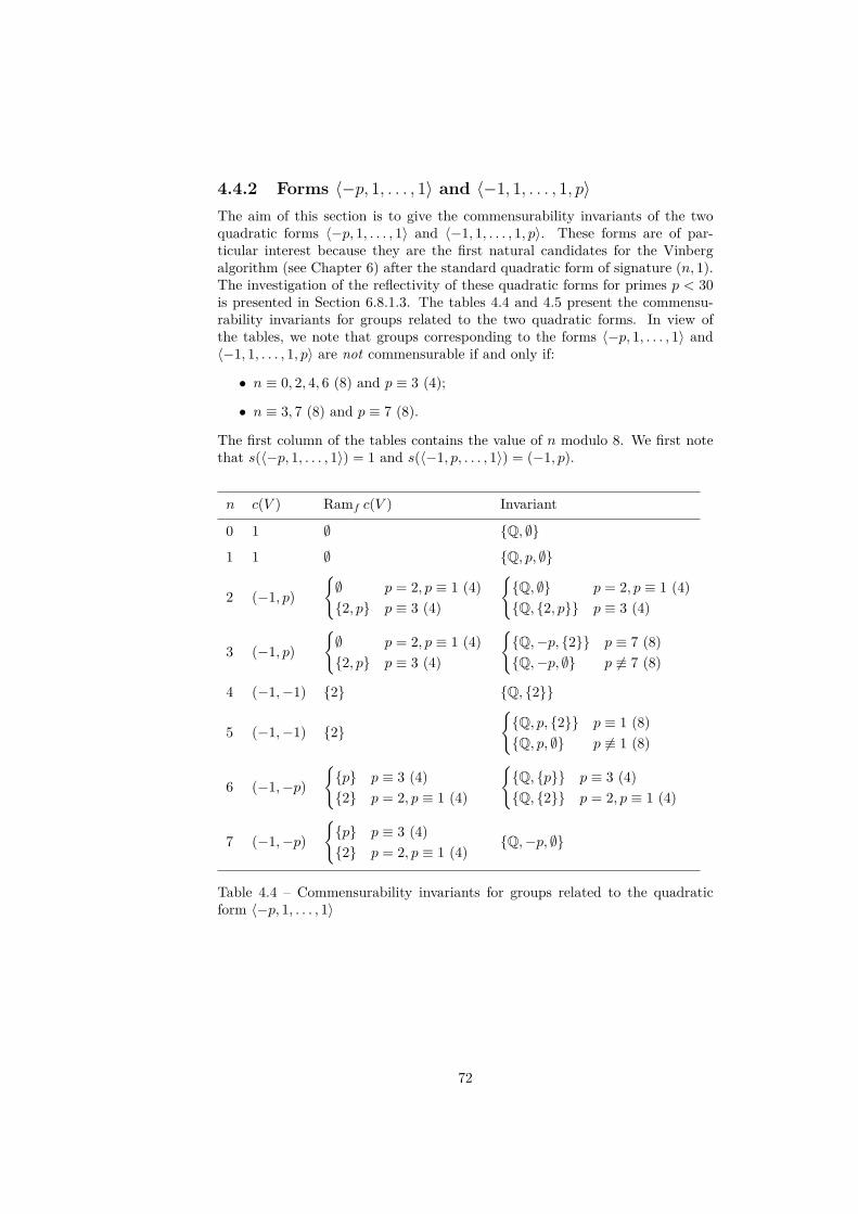
4.4.2 Forms 〈−p, 1, . . . , 1〉 and 〈−1, 1, . . . , 1, p〉The aim of this section is to give the commensurability invariants of the twoquadratic forms 〈−p, 1, . . . , 1〉 and 〈−1, 1, . . . , 1, p〉. These forms are of par-ticular interest because they are the first natural candidates for the Vinbergalgorithm (see Chapter 6) after the standard quadratic form of signature (n, 1).The investigation of the reflectivity of these quadratic forms for primes p < 30is presented in Section 6.8.1.3. The tables 4.4 and 4.5 present the commensu-rability invariants for groups related to the two quadratic forms. In view ofthe tables, we note that groups corresponding to the forms 〈−p, 1, . . . , 1〉 and〈−1, 1, . . . , 1, p〉 are not commensurable if and only if:
• n ≡ 0, 2, 4, 6 (8) and p ≡ 3 (4);
• n ≡ 3, 7 (8) and p ≡ 7 (8).
The first column of the tables contains the value of n modulo 8. We first notethat s(〈−p, 1, . . . , 1〉) = 1 and s(〈−1, p, . . . , 1〉) = (−1, p).
n c(V ) Ramf c(V ) Invariant
0 1 ∅ Q, ∅
1 1 ∅ Q, p, ∅
2 (−1, p)∅ p = 2, p ≡ 1 (4)2, p p ≡ 3 (4)
Q, ∅ p = 2, p ≡ 1 (4)Q, 2, p p ≡ 3 (4)
3 (−1, p)∅ p = 2, p ≡ 1 (4)2, p p ≡ 3 (4)
Q,−p, 2 p ≡ 7 (8)Q,−p, ∅ p 6≡ 7 (8)
4 (−1,−1) 2 Q, 2
5 (−1,−1) 2Q, p, 2 p ≡ 1 (8)Q, p, ∅ p 6≡ 1 (8)
6 (−1,−p)p p ≡ 3 (4)2 p = 2, p ≡ 1 (4)
Q, p p ≡ 3 (4)Q, 2 p = 2, p ≡ 1 (4)
7 (−1,−p)p p ≡ 3 (4)2 p = 2, p ≡ 1 (4)
Q,−p, ∅
Table 4.4 – Commensurability invariants for groups related to the quadraticform 〈−p, 1, . . . , 1〉
72
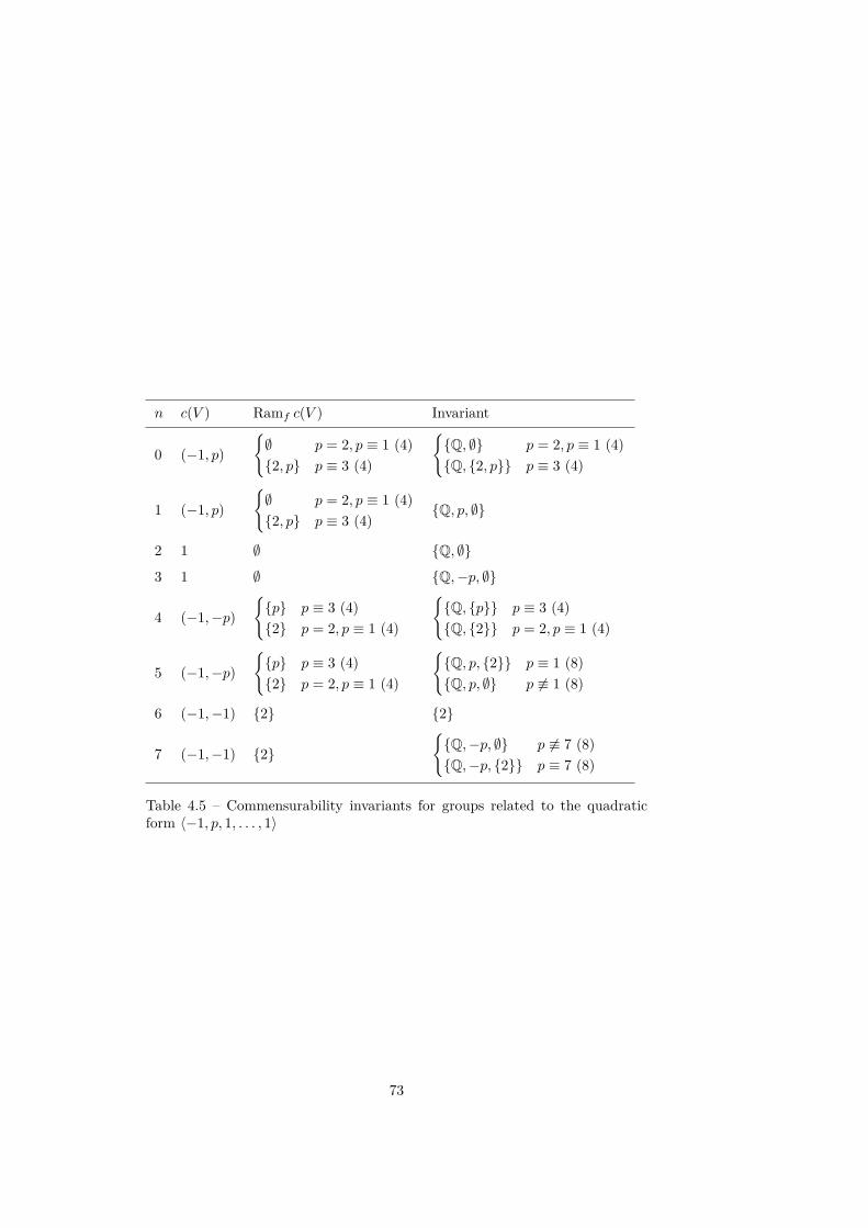
n c(V ) Ramf c(V ) Invariant
0 (−1, p)∅ p = 2, p ≡ 1 (4)2, p p ≡ 3 (4)
Q, ∅ p = 2, p ≡ 1 (4)Q, 2, p p ≡ 3 (4)
1 (−1, p)∅ p = 2, p ≡ 1 (4)2, p p ≡ 3 (4)
Q, p, ∅
2 1 ∅ Q, ∅
3 1 ∅ Q,−p, ∅
4 (−1,−p)p p ≡ 3 (4)2 p = 2, p ≡ 1 (4)
Q, p p ≡ 3 (4)Q, 2 p = 2, p ≡ 1 (4)
5 (−1,−p)p p ≡ 3 (4)2 p = 2, p ≡ 1 (4)
Q, p, 2 p ≡ 1 (8)Q, p, ∅ p 6≡ 1 (8)
6 (−1,−1) 2 2
7 (−1,−1) 2Q,−p, ∅ p 6≡ 7 (8)Q,−p, 2 p ≡ 7 (8)
Table 4.5 – Commensurability invariants for groups related to the quadraticform 〈−1, p, 1, . . . , 1〉
73

74

CHAPTER 5CoxIter
The aim of this chapter is to present CoxIter, a computer program which wedeveloped, whose purpose is to compute the invariants of hyperbolic Coxetergroups (for the theory, see sections 3.6 to 3.9). Most of the material presentedin this chapter was published in [Gug15]. The additional material consists ofthe following:
• Section 5.1 containing general information about the program.
• Some details and figures in Section 5.2, explaining the implementations ofthe algorithms.
• All information relating to the growth series and to the growth rate (inparticular in Section 5.2 and the part about the conjecture of Kellerhalsand Perren).
Consider the Coxeter subgroup Γ(14,1) of IsomH14 whose graph G is givenin Figure 5.1. If one wants to compute the covolume (or, equivalently, the Eulercharacteristic), the growth series and growth rate, the first step is to find thenumber of connected spherical subgraphs G. A careful (and painful) analysis ofthe graph shows that there exist 182 of them. The list of spherical subgraphsof G, which correspond to all faces of the polyhedron associated to Γ (exceptthe vertices at infinity), is too big to be determined by hand (there are 96001of them).
Figure 5.1 – The hyperbolic Coxeter group Γ(14,1) < IsomH14
The input of the program CoxIter is the graph of some hyperbolic Coxetergroup (see for example Section 5.4.1 for our group Γ(14,1)) together with someoptions. The output of CoxIter consists then of the following elements:
75

• CocompactnessWhether the group is cocompact or not.
• CofinitenessWhether the group has finite covolume or not.
• ArithmeticityIf the group is non-cocompact and has no dotted edge, we can decide ifthe group is arithmetic or not. If the group is non-cocompact and thegraph has dotted edges, it is necessary to know the weights of the dottededges (i.e. the length of the common perpendicular of the correspondinghyperplanes) to decide whether the group is arithmetic or not. In thissetting CoxIter prints the tests to decide the arithmeticity. If the group iscocompact, it is much more complicated to decide about the arithmeticity(see examples 4.4.1, 4.4.2 and 4.4.3) and the program does not handle thiscase.
• f -vector
• Euler characteristic
• SignatureIf the graph contains no dotted edge or if the weight of the dotted edgesare given, the signature is computed numerically1 using PARI.
• DimensionFor the cocompactness and cofiniteness tests, it is necessary to know thedimension of the hyperbolic space where the corresponding polyhedronlives. If this dimension is not provided, then the program will guess it2.
• Growth seriesThe rational expansion p(x)
q(x) of the growth series is given, where p(x) is aproduct of cyclotomic polynomials.
• Growth rateAn approximation of the growth rate is given. It is also checked if it is aPerron, a Pisot, or a Salem number.
For the group Γ(14,1), the output of CoxIter is the following (the denomi-nator of the growth series, which is a polynomial of degree 246 is not writtenhere for the sake of space):Reading file: ../ graphs /14- vinb85 . coxiter
Number of vertices : 17Dimension : 14Vertices : 1, 2, 3, 4, ..., 17Field generated by the entries of the Gram matrix : Q[
sqrt (2)]File read
1First, we compute numerical approximations of the roots and then we decide which arenegative, zero and positive.
2More precisely, it will assume that the dimension correspond to the maximal rank of aspherical or Euclidean subgraph.
76
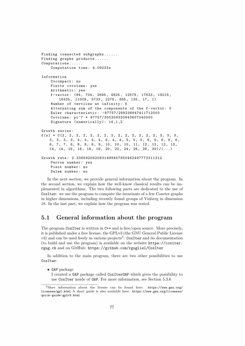
Finding connected subgraphs ......Finding graphs products ......Computations ......
Computation time: 4.09233 s
InformationCocompact : noFinite covolume : yesArithmetic : yesf- vector : (94, 704, 2695 , 6825 , 12579 , 17633 , 19215 ,
16425 , 11009 , 5733 , 2275 , 665, 135, 17, 1)Number of vertices at infinity : 5Alternating sum of the components of the f- vector : 0Euler characteristic : -87757/289236647411712000Covolume : pi^7 * 87757/305359330843607040000Signature ( numerically ): 14,1,2
Growth series :f(x) = C(2, 2, 2, 2, 2, 2, 2, 2, 2, 2, 2, 2, 2, 2, 3, 3, 3,
3, 3, 3, 3, 4, 4, 4, 4, 4, 4, 4, 5, 5, 5, 6, 6, 6, 6, 6,6, 7, 7, 8, 8, 8, 9, 9, 10, 10, 10, 11, 12, 12, 12, 13,14, 14, 15, 16, 18, 18, 20, 22, 24, 26, 28, 30) /(...)
Growth rate: 2.3365920620831499457950462497773311312Perron number : yesPisot number : noSalem number : no
In the next section, we provide general information about the program. Inthe second section, we explain how the well-know classical results can be im-plemented in algorithms. The two following parts are dedicated to the use ofCoxIter: we use the program to compute the invariants of a few Coxeter graphsin higher dimensions, including recently found groups of Vinberg in dimension18. In the last part, we explain how the program was tested.
5.1 General information about the programThe program CoxIter is written in C++ and is free/open source. More precisely,it is published under a free license, the GPLv3 (the GNU General Public Licensev3) and can be used freely in various projects3. CoxIter and its documentation(to build and use the program) is available on the website https://coxiter.rgug.ch and on GitHub: https://github.com/rgugliel/CoxIter
In addition to the main program, there are two other possibilities to useCoxIter:
• GAP packageI created a GAP package called CoxIterGAP which gives the possibility touse CoxIter inside of GAP. For more information, see Section 5.3.6
3More information about the license can be found here: https://www.gnu.org/licenses/gpl.html A short guide is also available here: https://www.gnu.org/licenses/quick-guide-gplv3.html
77

• CoxIterWebA web version of CoxIter, which can be used via any web-browser, canbe downloaded and installed on any server. The source code is on myGitHub account: https://github.com/rgugliel/CoxIterWebAlternatively, a demo version can be found here: https://coxiter.rafaelguglielmetti.ch/ Hence, you can use CoxIter from anywherefor small groups (generated by at most 20 reflections).
5.1.1 VersionsThe first version of the program, CoxIter 1.0.0, was published in [Gug15]. Afterthat, more versions were released:
• 1.0.1Correction of a small bug.
• 1.0.2Correction of a bug causing incorrect answer in the cofiniteness test.
• 1.1This version added the following features:
– growth series and growth rate;– test for the growth rate (Perron, Pisot and Salem numbers);– numerical computation of the signature;– more formats for the output (LATEX, PARI);– guess the dimension if it is not specified;– speed-up of some computations.
• 1.1.1This function brought the following features:
– ability to read a file directly;– ability to export the graph;– GAP format for the output;– display some help at start-up if no file is given.
• 1.2This function brought the following features:
– correction of a bug;– fully functional Windows and OSX versions.
5.1.2 External libraries usedCoxIter is developed in C++11. Moreover, it requires the following externallibraries:
GMP (or GNU Multiple Precision Arithmetic Library) is a free library forarbitrary precision arithmetic with integers.
78

OpenMP This API allows CoxIter to parallelize some parts of the computa-tions and speed-up the execution. It is not mandatory.
PARI We use the C library PARI to compute the signature of the group, thegrowth rate and to determine whether it is a Perron, Pisot or Salem num-bers. It is not mandatory but if it is not available, then CoxIter willcompute only the growth series and not the growth rate (and won’t beable to compute the signature).
PCRE The PCRE library (PCRE - Perl Compatible Regular Expressions) isused to parse the user input (parameters of the program and CoxIterfiles).
5.1.3 Design descriptionWe briefly explain the main steps of the working flow of CoxIter. Dependingon the given parameters, some steps may be skipped.
• Reading the parametersWhen the program is launched, it first lists all the given parameters (thefile to read and the options for the computations). This is done in theApp::bReadMainParameters function.
• Reading the graphThe Coxeter graph is read from the file (CoxIter::bReadGraphFromFile)and some initializations are made (memory allocation, field generated bythe entries of the Gram matrix, some vertices may be removed).
• First outputsBefore the computations, we may have to print the first informations:Gram matrix, Coxeter matrix, writing the graph in a file, drawing of theCoxeter graph.
• Finding connected spherical and Euclidean subgraphsWe find all connected spherical and Euclidean subgraphs of the givenCoxeter graph (see Section 5.2.1 for more information).
• Partial non-cofiniteness testA partial non-cofiniteness test4 has been implemented, mostly for its useinside the Vinberg algorithm (see Section 6.3.3.1 for more information),and can be thousand times faster than the complete cofiniteness test.
• Graph productsAll the possible products (spherical and Euclidean) are computed andcounted. If CoxIter has to perform the cocompactness and cofinitenesstests, some of them are stored (for each component of the product we keepthe type of the graph and the list of the vertices).
• Cofiniteness test
• Euler characteristic and f -vector4If the output of the test is "true", then it is certain that the group is not cofinite. If the
answer is "false", then we cannot say anything and have to perform the complete cofinite test.
79
• Compactness and arithmeticity tests
• Other computationsThe following are computed: growth series, growth rate (and Perron, Pisotand Salem tests) and signature.
• OutputThe results of the computations and tests are printed.
5.1.3.1 Different files
We list all the files in the project and their main features.
app Main file for the execution of the program.
arithmeticity Function to recursively delete separating edges the queues ofthe graph (see Proposition 3.9.14) and to test the arithmeticity.
coxiter All global functions to do the input/output, manage the graph andmost of the computations.
graph To describe one graph: list of its vertices, adjacent vertices of the graph,test of inclusion.
graphs.list Allows to store and browse all graphs of one type (spherical orEuclidean).
graph.list.iterator Allows to go through the list of graphs in a sequentialorder.
graphs.list.n All graphs of a given rank.
graphs.product & graphs.product.set Store one product of graphs.
growthrate The compute the growth rate and do the Perron, Pisot and Salemtests (the PARI library is needed).
index2 To create the index two subgroup (see Proposition 7.1.9).
signature Numerical computation of the signature.
lib/maths_tools Some mathematical functions: integer square root, list ofdivisors, prime factors and prime decomposition, ...
lib/numbers/number_rational To handle computations with rational num-bers.
lib/polynomials Divisibility and division of polynomials, product by symbols5
and list of cyclotomic polynomials.
5.2 AlgorithmsLet (Γ, S) be a hyperbolic Coxeter group of rank r. In what follows, we use thenotations of the program. In particular, the r vertices of the Coxeter graph arelabelled 0, . . . , r − 1 instead of 1, . . . , r.
5Recall that, for a positive integer k, the symbol [k] is the polynomial 1 + x+ . . .+ xk−1.
80

5.2.1 Euler characteristic and f-vectorWe present here the main steps for the computation of the Euler characteristicχ (see Section 3.7) and the f -vector. These steps are the following:
(1) We find all paths (simple walks with all edges labelled with a 3) startingfrom every vertex, that is, every Am. Note that a single vertex is such apath.
(2) We extend these paths in order to find the finite and affine irreducibleCoxeter subgroups.
(3) We compute all the possible products of groups.
(4) We count these products with their orders and multiplicities. The Eulercharacteristic is then computed with Proposition 3.7.1 (by taking into ac-count the orders of finite irreducible spherical Coxeter groups in Table 3.2).
Note that using (1)− (3), and by theorems 3.7.5 and 3.7.6, we can compute thef -vector of Γ.
First, we use a depth-first search algorithm to explore the graph from everyvertex and to find any subgraph of type Am (function CoxIter::DFS). For eachsuch Am, we try to extend it to other connected spherical and Euclidean graphs(function CoxIter::addGraphsFromPath).Once the connected graphs are found, we compute all the possible products.Counting them with their multiplicities gives the f -vector and the Euler char-acteristic.
Figure 5.2 – Extending paths to graphs
5.2.2 Growth series and growth rateWe want to compute the growth series fΓ of Γ. Using Steinberg’s formula, wecan write
1fΓ(x) =
∑T∈F
(−1)|T |
fT (x−1) ,
where F =T ⊂ S : |ΓT | < ∞
. If T ⊂ S corresponds to the finite subgroup
ΓT , then we can write ΓT =∏li=1 Γi, where each Γi is a finite and irreducible
81
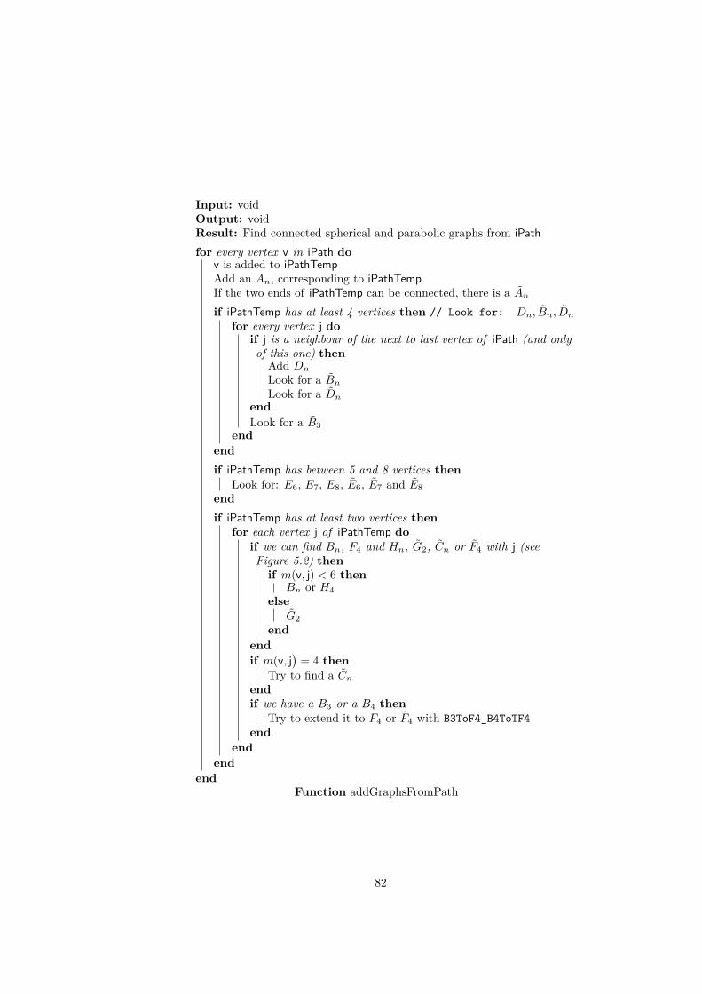
Input: voidOutput: voidResult: Find connected spherical and parabolic graphs from iPathfor every vertex v in iPath do
v is added to iPathTempAdd an An, corresponding to iPathTempIf the two ends of iPathTemp can be connected, there is a Anif iPathTemp has at least 4 vertices then // Look for: Dn, Bn, Dn
for every vertex j doif j is a neighbour of the next to last vertex of iPath (and onlyof this one) then
Add Dn
Look for a BnLook for a Dn
endLook for a B3
endendif iPathTemp has between 5 and 8 vertices then
Look for: E6, E7, E8, E6, E7 and E8endif iPathTemp has at least two vertices then
for each vertex j of iPathTemp doif we can find Bn, F4 and Hn, G2, Cn or F4 with j (seeFigure 5.2) thenif m(v, j) < 6 then
Bn or H4else
G2end
endif m(v, j
)= 4 then
Try to find a Cnendif we have a B3 or a B4 then
Try to extend it to F4 or F4 with B3ToF4_B4ToTF4end
endend
endFunction addGraphsFromPath
82
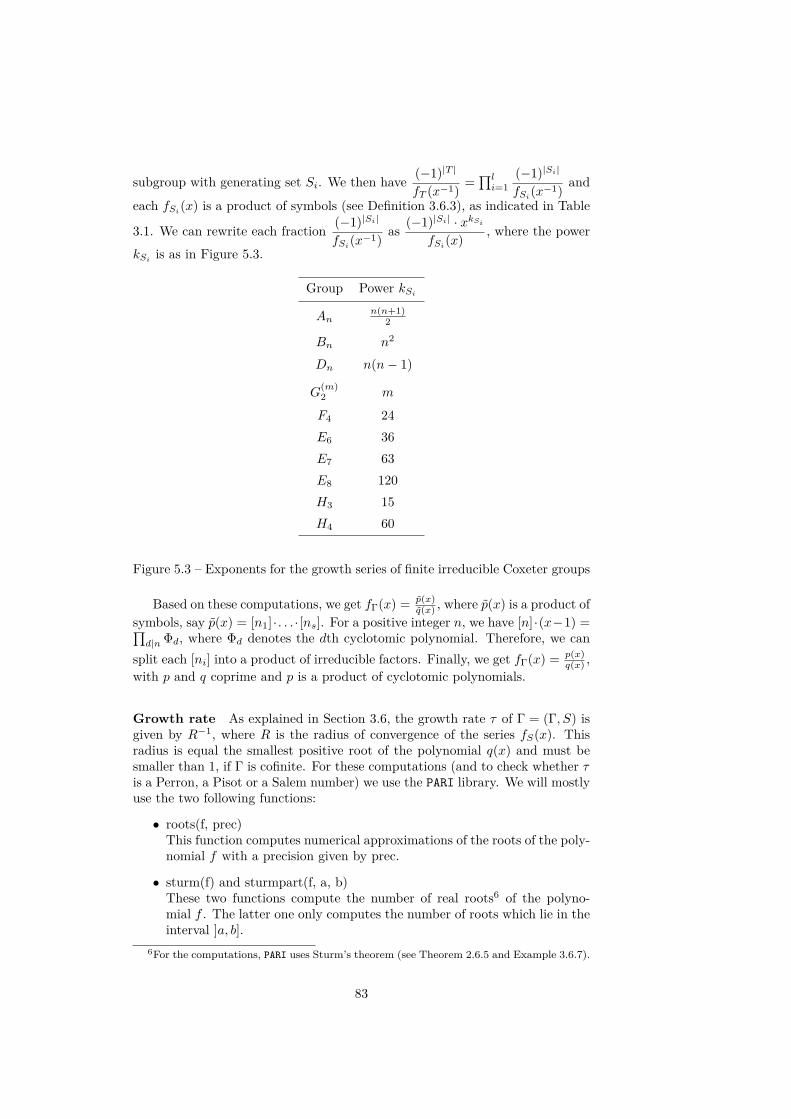
subgroup with generating set Si. We then have (−1)|T |
fT (x−1) =∏li=1
(−1)|Si|
fSi(x−1) and
each fSi(x) is a product of symbols (see Definition 3.6.3), as indicated in Table
3.1. We can rewrite each fraction (−1)|Si|
fSi(x−1) as (−1)|Si| · xkSifSi(x) , where the power
kSi is as in Figure 5.3.
Group Power kSi
Ann(n+1)
2
Bn n2
Dn n(n− 1)
G(m)2 m
F4 24E6 36E7 63E8 120H3 15H4 60
Figure 5.3 – Exponents for the growth series of finite irreducible Coxeter groups
Based on these computations, we get fΓ(x) = p(x)q(x) , where p(x) is a product of
symbols, say p(x) = [n1] · . . . · [ns]. For a positive integer n, we have [n] ·(x−1) =∏d|n Φd, where Φd denotes the dth cyclotomic polynomial. Therefore, we can
split each [ni] into a product of irreducible factors. Finally, we get fΓ(x) = p(x)q(x) ,
with p and q coprime and p is a product of cyclotomic polynomials.
Growth rate As explained in Section 3.6, the growth rate τ of Γ = (Γ, S) isgiven by R−1, where R is the radius of convergence of the series fS(x). Thisradius is equal the smallest positive root of the polynomial q(x) and must besmaller than 1, if Γ is cofinite. For these computations (and to check whether τis a Perron, a Pisot or a Salem number) we use the PARI library. We will mostlyuse the two following functions:
• roots(f, prec)This function computes numerical approximations of the roots of the poly-nomial f with a precision given by prec.
• sturm(f) and sturmpart(f, a, b)These two functions compute the number of real roots6 of the polyno-mial f . The latter one only computes the number of roots which lie in theinterval ]a, b].
6For the computations, PARI uses Sturm’s theorem (see Theorem 2.6.5 and Example 3.6.7).
83
For the computations, we fix a small number ε > 0 (typically, ε = 10−50)which should be big compared to the precision used to compute the roots (typ-ically we do the computations with 57 decimals on 32 bits computers and 115decimals on 64 bits computers). For each root, we decide that the root is realif its imaginary part is smaller than ε. Notice that since we know the exactnumber of real roots, approximation errors are not a problem: if we detect toomany real roots, then we increase the precision and choose a smaller ε and doagain the computations. We then can pick the smallest positive root R and itsinverse τ (again, we do not have to worry about approximation errors: if tworoots r1 and r2 are such that |r1 − r2| < ε, then we can increase the precisionand choose a smaller ε). We also pick the corresponding irreducible factor g(x)of q(x) and we let g(x) = xdeg g ·g
(x−1). Observe that g is monic and irreducible
which mean that g is the minimal polynomial of the algebraic integer τ .
Properties of the growth rate Once we get the growth rate and its minimalpolynomial we try to determine whether it is a Perron, a Salem or a Pisotnumber.
To decide whether τ is a Perron number or not, we only have to check ifevery negative root r of g satisfies |r| < τ . We then have the following threepossibilities:
• For every such root r we have |r|+ ε < τThen we know that τ is a Perron number.
• There exists r such that |r| − ε < τ < |r|+ εWe have to increase the precision in order to conclude.
• Otherwiseτ is not a Perron number.
As pointed out above, checking whether λ is a Pisot number is easy and, asusual, we display a warning if we cannot decide (up to ε) whether a root haveabsolute value smaller than one or not.
We now come to the last point: deciding whether τ is a Salem number ornot. A necessary condition for τ to be a Salem number is that its minimalpolynomial g is a self-reciprocal polynomial with deg g even. If it is the case,it remains to verify that (deg g − 2) roots of g lie on S1, the unit circle. Weuse the Möbius transformation h(t) = t−i
t+i of C to send R ∪ ∞ to S1 and weconsider g(t) := g h(t) and the polynomial G(t) := (t+ i)deg g · g(t). Since g isirreducible, we have |Rg∩S1| = |Rg∩R| = |RG∩R|, where Rp denotes the set ofcomplex roots of the polynomial (or rational function) p. We remark that sinceg is self-reciprocal, then G(t) is a real polynomial and we can use the sturmfunction of PARI to compute the number of its real roots. For computationalpurpose, we give an explicit description of G(t). For that, we will need thefollowing two identities:
(t+ i)2l + (t− i)2l = 2 ·l∑
k=0
(2l2k
)· t2k · (−1)l−k,
(t+ i)2l+1 + (t− i)2l+1 = 2 ·l∑
k=0
(2l + 12k + 1
)· t2k+1 · (−1)l−k.
84

We write G(t) =∑mj=0 ajt
j and we distinguish two cases. When m is even, wehave
G(t) = am/2 · (t2 + 1)m2 +m2 −1∑j=0
aj ·((z − i)j(z + i)m−j + (z − i)m−j(z + i)j
)= am/2 · (t2 + 1)m2 +
m2 −1∑j=0
aj(z2 + 1)j ·((z + i)m−2j + (z − i)m−2j)
= am/2 · (t2 + 1)m2 + 2m2 −1∑j=0
aj(z2 + 1)j ·m2 −j∑k=0
(m− 2j
2k
)t2k · (−1)m2 −j−k.
When m is odd, we find
G(t) = 2 ·m−1
2∑j=0
aj(z2 + 1)j ·m−1
2 −j∑k=0
(m− 2j2k + 1
)· t2k+1 · (−1)
m−12 −j−k.
5.2.3 ArithmeticityTo check the arithmeticity of a given Coxeter group, we use Proposition 3.9.14.The code for the test is in the Arithmeticity class.
First, we check if the graph contains no dotted edge, if it is non-cocompactand if all the edge labels m(s, t) lie in the set ∞, 2, 3, 4, 6. These verifica-tions are done in the beginning of the Arithmeticity::test function. Atthis point, we know that the coefficients of the matrix 2 · G can take thevalues
0,−1,−2, 2,−
√2,−√
3. We then use multiple calls to the function
Arithmeticity::collapseQueues to recursively delete separating edges of thegraph (regardless of the labels which appear in these paths) to reduce the com-putation time of the determination of the cycles.For each vertex v, we look for simple cycles passing through v (note that we onlylook at cycles which contain vertices j with v ≤ j to avoid multiple counting ofthe graphs). This is done by calling Arithmeticity::findCycles(v,v). Foreach cycle, we check whether the number of edges labeled with 4 and 6 respec-tively along the cycle is even (labels 3 and∞ are not an obstacle to arithmeticityat this point).
As explained in Remark 3.9.15, if the graph contains dotted lines, we need todetermine all the relevant entries of the Gram matrix in order to decide aboutthe arithmeticity of the group. In this case, CoxIter will indicate what are theconditions for the group to be arithmetic. The program would give conditionsin the following way:l1m3: weight of the dotted line between hyperplanes 2 and 4l0m5: weight of the dotted line between hyperplanes 1 and 6
The group is arithmetic if and only if all the followingvalues lie in Z:
4 * l1m3 ^24 * l0m5 ^22^3 * l1m3 * l0m5
85

Input: iRoot: starting vertex for the searchiFrom: previous vertex (or iRoot if it is a non-recursive call of thefunction)
Output: voidResult: Look for simple cycles passing through iPath[0]Add the vertex iRoot to the pathfor every neighbour i of iRoot with i ≥ iPath[0] do
if the edge ( i,iFrom) was not visited thenif i == iPath[0] then
This is a simple cycle. Use testCycle to test it.endelse if i is not a vertex of iPath then
Mark the edge (iRoot,i) as visitedCall findCycles(i,iRoot)
endend
Function findCycles
5.2.4 Linearization of a (sparse) symmetric matrixIt is possible to give the values of the dotted lines (i.e. the corresponding entriesof the Gram matrix) to CoxIter. These values will be used for the output (forexample when printing the Gram matrix), the results of the arithmeticity testor for the computation of the signature. Since the Gram matrix is symmetricand because these values are not always given and are rarely used, we want tostore them in a vector instead. We start with an r × r matrix with rows andcolumns labelled 0, . . . , r − 1 and we want to induce a bijection
ι : 0, . . . , r − 12 −→
0, . . . , r(r + 1)2 − 1
.
We will enumerate the elements of the first row 0, . . . , r − 1, the ones of thesecond row r, . . . , 2r − 2, etc. Now, if the pair (i, j), where 0 ≤ i < j ≤ r − 1,designates an element of the matrix, its index ι(i, j) in the vector is given by
ι(i, j) = i(2r − 1− i)2 + j.
Conversely, if k ∈
0, . . . , r(r+1)2 − 1
is the index of an element of the vector,
then the corresponding entry of the matrix is on the row
row(k) = floor(2r + 1)−
√(2r + 1)2 − 8k2 ,
and column
col(k) = k −row(k) ·
(2r − 1− row(k)
)2
Finally, note that with this process, we can then use a map[int, String]to store only the existing values.
86
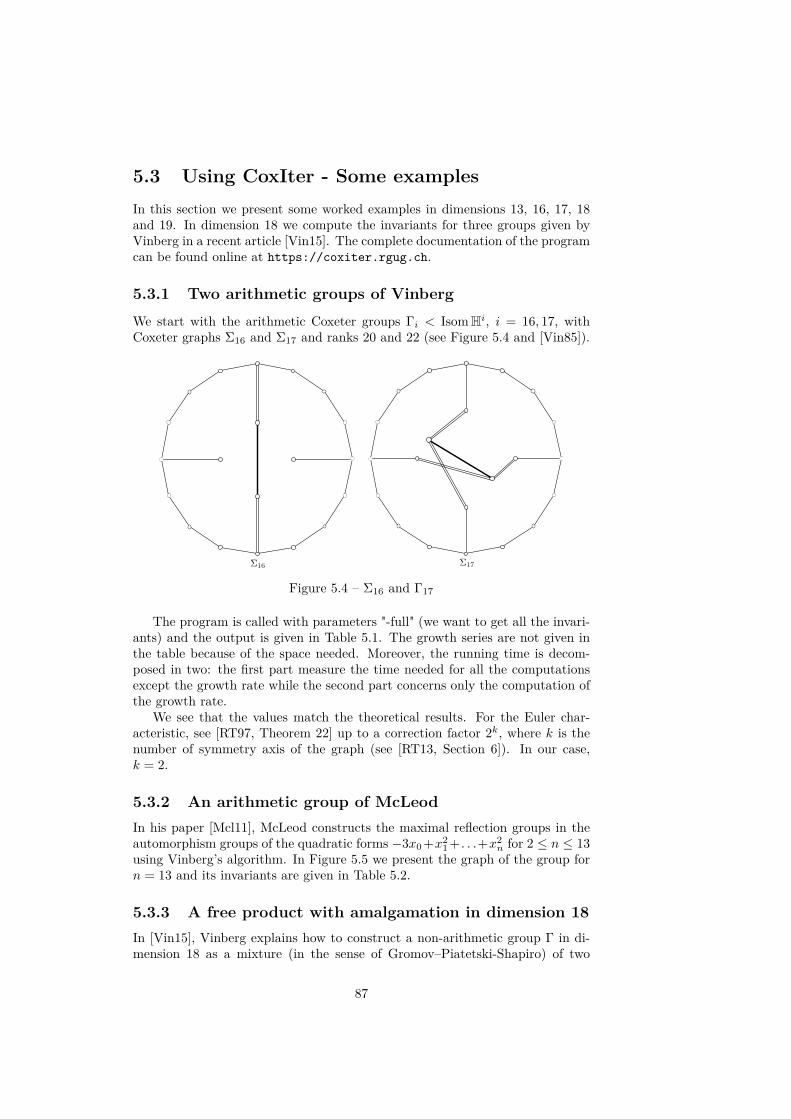
5.3 Using CoxIter - Some examplesIn this section we present some worked examples in dimensions 13, 16, 17, 18and 19. In dimension 18 we compute the invariants for three groups given byVinberg in a recent article [Vin15]. The complete documentation of the programcan be found online at https://coxiter.rgug.ch.
5.3.1 Two arithmetic groups of VinbergWe start with the arithmetic Coxeter groups Γi < IsomHi, i = 16, 17, withCoxeter graphs Σ16 and Σ17 and ranks 20 and 22 (see Figure 5.4 and [Vin85]).
Figure 5.4 – Σ16 and Γ17
The program is called with parameters "-full" (we want to get all the invari-ants) and the output is given in Table 5.1. The growth series are not given inthe table because of the space needed. Moreover, the running time is decom-posed in two: the first part measure the time needed for all the computationsexcept the growth rate while the second part concerns only the computation ofthe growth rate.
We see that the values match the theoretical results. For the Euler char-acteristic, see [RT97, Theorem 22] up to a correction factor 2k, where k is thenumber of symmetry axis of the graph (see [RT13, Section 6]). In our case,k = 2.
5.3.2 An arithmetic group of McLeodIn his paper [Mcl11], McLeod constructs the maximal reflection groups in theautomorphism groups of the quadratic forms −3x0 +x2
1 + . . .+x2n for 2 ≤ n ≤ 13
using Vinberg’s algorithm. In Figure 5.5 we present the graph of the group forn = 13 and its invariants are given in Table 5.2.
5.3.3 A free product with amalgamation in dimension 18In [Vin15], Vinberg explains how to construct a non-arithmetic group Γ in di-mension 18 as a mixture (in the sense of Gromov–Piatetski-Shapiro) of two
87

Invariant Σ16 Σ17
Cocompact no noFinite covolume yes yesArithmetic yes yesf -vector (325, 2804, 11914, 33164,
67410, 105462, 130646,130062, 104670, 68042,35490, 14658, 4690, 1122,189, 20, 1)
(807, 7586, 33960, 98184,206120, 332982, 427584,444428, 377232, 262050,148500, 68076, 24884, 7089,1518, 230, 22, 1)
Euler charact. 6423321792360171042879569920000 0
Growth rate τ 2.70239585907681598724 3.26561859868532761547Is τ Perron yes yesRunning time 0.6s + 10.5s 2.7s + 15s
Table 5.1 – Output of CoxIter for Σ16 and Σ17
Invariant ValueCocompact noFinite covolume yesf -vector (413, 2964, 10238, 22761, 36024, 42265, 37380, 25005,
12556, 4641, 1218, 213, 22, 1)Euler characteristic 0Growth rate τ 7.0978514419211704695935654214851191548Is τ Perron yesRunning time 0.18s + 7s
Table 5.2 – Output of CoxIter for the reflection group corresponding to theautomorphism group of the quadratic form −3x0 + x2
1 + . . . + x213 (see Figure
5.5)
non-commensurable arithmetic hyperbolic Coxeter groups Γ1 and Γ2. Geomet-rically, the two associated polyhedra P1 and P2 of the groups Γ1,Γ2 < IsomH18
have an isometric facet P0. In this setting, the associated polyhedron P of Γis the gluing of P1 and P2 along their common facet P0. From an algebraicpoint of view, the group Γ is the free product with amalgamation given byΓ = ∆1 ?Γ0 ∆2, where ∆i is the subgroup of Γi generated by all the generatorsof Γi except the one corresponding to the hyperplane containing the facet P0.
We use CoxIter to compute the invariants of the groups Γ1,Γ2 and Γ andwe check that the covolume of Γ is indeed the sum of the covolumes of the twocomponents. We also compute the growth series of ∆1 and ∆2 and we checkthat 1
fΓ= 1
f∆1+ 1
f∆2− 1
fΓ0(see [Alo91, Theorem 2]).
Remark 5.3.1The polyhedron P obtained by glueing (or, equivalently the free product withamalgamation Γ = ∆1 ?Γ0 ∆2) is not necessarily Coxeter. However, if the facetP0 is perpendicular to every adjacent facet, then the result will be of Coxetertype.
88

Figure 5.5 – Group of reflections related to automorphism group of the quadraticform −3x0 + x2
1 + . . .+ x213
5.3.3.1 First component of the product
Information for the construction of the first component Γ1 of the product aregiven in [KV78] and [Vin15]. The generators s1, . . . , s37 of Γ1 are given by theroots of a certain integral lattice L1 (in fact, L1 is the unique odd unimodularquadratic lattice of signature (18, 1)).
Figure 5.6 – Construction of Γ1 < IsomH18 - First component of the product
We use the terminology and present the results of [KV78]. There are 22 longroots (i.e. roots of norm 2) and 15 short roots (i.e. roots of norm 1). The actionof the symmetry group of the graph (which is isomorphic to S4, see below) splitsthe short roots into two orbits of size 3 and 12. The 3 roots are called roots ofthe first kind while the 12 other elements are called roots of the second kind. Thediagram Σ∗ of the long roots is presented in Figure 5.6(a). If we consider the 6"long edges" (or "tetrahedral edges") of Figure 5.6(b), then each pair of oppositeedges gives rise to a root of the first kind. Hence, we get the three vertices of thefirst kind 18, 25, 26 connected respectively to vertices (17, 22), (1, 9) and (5, 13)
89

by a double edge. The figure 5.6(c) depicts the connection of one vertex of thesecond kind with the graph Σ∗. We then let the symmetry group of Σ∗ (see be-low) act on the triple of vertices (1, 20, 24) and find 11 other triples, correspond-ing to the 11 others vertices of the second kind. The 12 triples of vertices arethe following: (1, 20, 24), (1, 6, 12), (5, 16, 20), (5, 10, 21), (9, 16, 19), (9, 4, 14),(13, 2, 8), (13, 19, 24), (17, 2, 10), (17, 4, 12), (22, 8, 21), (22, 6, 14). Now, verticesof the first kind are connected among themselves by lines labelled with an ∞while vertices of the second kind are connected among themselves by dottededges. Each vertex of the first kind is connected to each vertex of the secondkind either by an ∞ or by a dotted edge according to the rule explained in[KV78, Section 2]. We finally found a Coxeter graph Σ(Γ1) with 37 vertices and171 edges. When given to CoxIter, it produces the output given in Table 5.3.
Invariant ValueCocompact noFinite covolume yesf -vector (3839, 37842, 177812, 540624, 1197240, 2050008,
2807602, 3135528, 2883540, 2189924, 1369854, 700352,288801, 94113, 23497, 4282, 525, 37, 1)
Euler characteristic − 10963885484922028263066875985920000
Volume 1096388548491482580623111880900608000000 · π
9
Growth rate τ 16.976062922983291305757316760341665593Is τ Perron yesRunning time 55s + 20s
Table 5.3 – Output of CoxIter for Γ1
Remark 5.3.2Using AlVin (see Chapter 6) it is also possible to compute directly the 37 normalvectors of polyhedron P1 and the presentation of its reflection group Γ1. Thecomputations take approximatively 2-3 minutes on a desktop computer.
Lemma 5.3.3 ([KV78])The symmetry group of the graph Σ(Γ1) is isomorphic to S4.
Proof. To determine the symmetry group of the graph of the group Γ1 we firstcompute the group of symmetries sym Σ∗ of the graph Σ∗, presented in Fig-ure 5.6. It is easy to see that any automorphism σ ∈ sym Σ∗ is completelydetermined by the images of the middle-points of two adjacent long edges (forexample the images of the vertices 22 and 1). There are 6 possibilities for theimages of 22 and four possibilities for the vertex 1, corresponding to the fouradjacent long edges of the image of 22. Hence, the group sym Σ∗ has order 24.We consider the automorphisms
σ1 = (22 9) (1 17)σ2 = (1 5) (9 13)σ3 = (22 1) (9 17)
90

and we see that σ1 σ2 has order 3, σ2 σ3 has order 3 and σ1 σ3 has order 2.Therefore, sym Σ∗ = S4.By a lemma of [KV78], every element of sym Σ∗ can be extended to an elementof sym Σ, where Σ denotes the graph of the group Γ1. Conversely, since Σ \Σ∗contains two complete graphs K12 and K3 (here, Kl denotes the complete graphwith l vertices and
(l2)edges), any element of sym Σ must preserve the subgraph
Σ∗. We thus have a surjective restriction map res : sym Σ −→ sym Σ∗. Sincethis map is also injective we have sym Σ = S4.
5.3.3.2 Second component of the product
The lattice for the second group is L2 = L0 ⊕ Ze ⊂ R18,1, where:
• L0 is the unique even unimodular quadratic lattice of signature (17, 1).Its maximal subgroup generated by reflections is Γ0, the hyperbolic Cox-eter group whose associated fundamental polyhedron is P0, which is thecommon facet of P1 and P2.
• e is a long root of square norm 2.
The graph of the group Γ2 < IsomH18 is presented in Figure 5.7 and itsresulting invariants in Table 5.4.
Figure 5.7 – Γ2 < IsomH18 - Second component of the product
5.3.3.3 Amalgamated product
As described above, we want to construct the amalgamated product of thegroups ∆1 and ∆2. We see that they have a common hyperbolic subgroup Γ0of signature (17, 1, 1) (see Figure 5.8). The hyperplane in H18 which containsthe associated polyhedron P0 is the one corresponding to the black dot in thegraphs of Γ1 and Γ2.
A presentation for the product Γ = ∆1 ?Γ0 ∆2 is obtained as follows.
• Start with the presentation of Γ1 = 〈s1, . . . , s37|(si · sj)mij 〉.
91
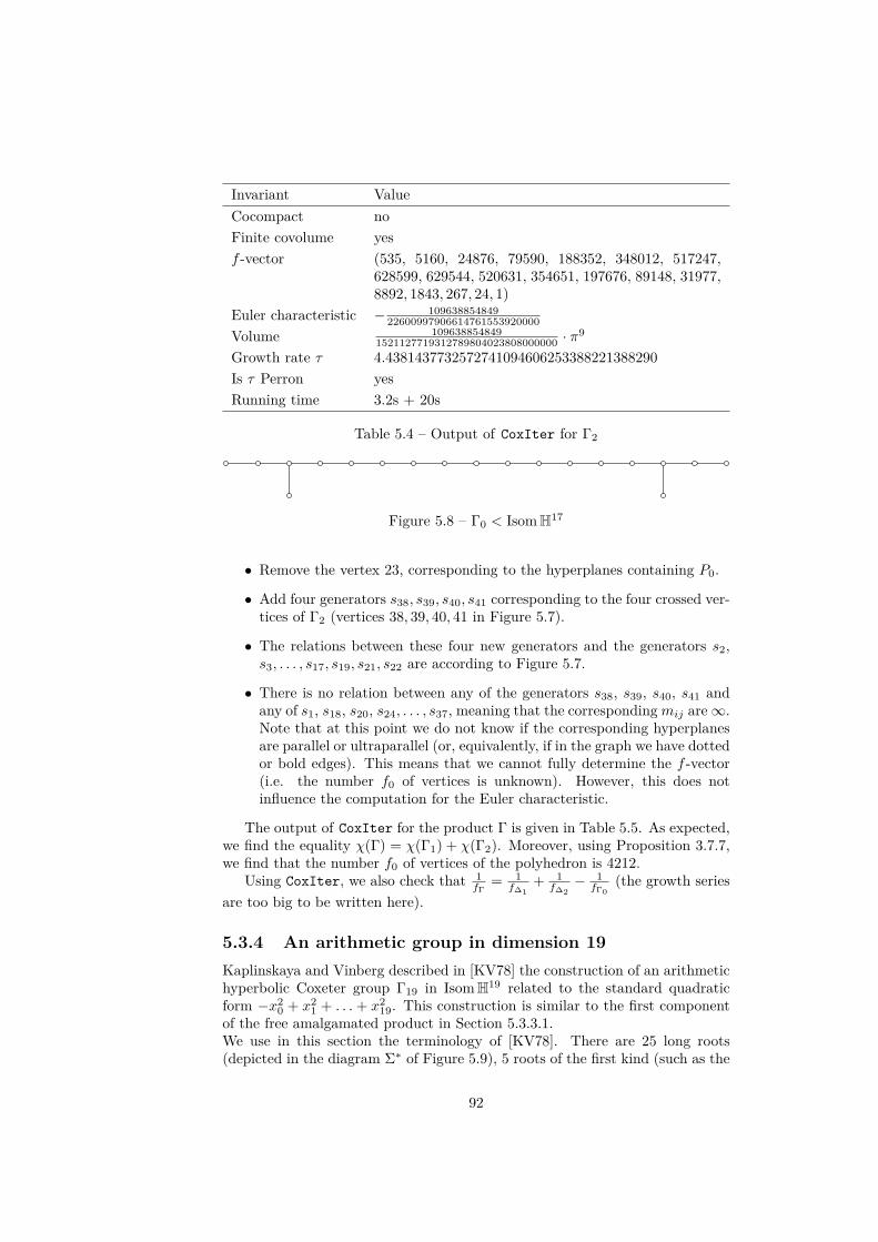
Invariant ValueCocompact noFinite covolume yesf -vector (535, 5160, 24876, 79590, 188352, 348012, 517247,
628599, 629544, 520631, 354651, 197676, 89148, 31977,8892, 1843, 267, 24, 1)
Euler characteristic − 10963885484922600997906614761553920000
Volume 1096388548491521127719312789804023808000000 · π
9
Growth rate τ 4.4381437732572741094606253388221388290Is τ Perron yesRunning time 3.2s + 20s
Table 5.4 – Output of CoxIter for Γ2
Figure 5.8 – Γ0 < IsomH17
• Remove the vertex 23, corresponding to the hyperplanes containing P0.
• Add four generators s38, s39, s40, s41 corresponding to the four crossed ver-tices of Γ2 (vertices 38, 39, 40, 41 in Figure 5.7).
• The relations between these four new generators and the generators s2,s3, . . . , s17, s19, s21, s22 are according to Figure 5.7.
• There is no relation between any of the generators s38, s39, s40, s41 andany of s1, s18, s20, s24, . . . , s37, meaning that the correspondingmij are∞.Note that at this point we do not know if the corresponding hyperplanesare parallel or ultraparallel (or, equivalently, if in the graph we have dottedor bold edges). This means that we cannot fully determine the f -vector(i.e. the number f0 of vertices is unknown). However, this does notinfluence the computation for the Euler characteristic.
The output of CoxIter for the product Γ is given in Table 5.5. As expected,we find the equality χ(Γ) = χ(Γ1) + χ(Γ2). Moreover, using Proposition 3.7.7,we find that the number f0 of vertices of the polyhedron is 4212.
Using CoxIter, we also check that 1fΓ
= 1f∆1
+ 1f∆2− 1
fΓ0(the growth series
are too big to be written here).
5.3.4 An arithmetic group in dimension 19Kaplinskaya and Vinberg described in [KV78] the construction of an arithmetichyperbolic Coxeter group Γ19 in IsomH19 related to the standard quadraticform −x2
0 + x21 + . . . + x2
19. This construction is similar to the first componentof the free amalgamated product in Section 5.3.3.1.We use in this section the terminology of [KV78]. There are 25 long roots(depicted in the diagram Σ∗ of Figure 5.9), 5 roots of the first kind (such as the
92

Invariant Valuef -vector (4212, 41464, 195047, 594510, 1321044, 2271012,
3123717, 3503919, 3235974, 2467015, 1548147, 793376,327561, 106710, 26575, 4814, 583, 40, 1)
Euler characteristic − 86614695330711738538300508827811840000
Volume 8661469533071117009824562522292617216000000 · π
9
Growth rate τ 20.082709777287151523318262297132352789Is τ Perron yesRunning time 74s + 29s
Table 5.5 – Output of CoxIter for Γ
vertex 19 in Figure 5.9(b)) and 20 roots of the second kind (such as the vertex24 in Figure 5.9(c)). In order to explain how to connect the vertices of the firstand second kind to the graph Σ∗ we first compute the automorphism group ofthe graph Σ∗.
Figure 5.9 – Construction of Γ19 < IsomH19
Lemma 5.3.4 ([KV78])The automorphism group of Σ∗ is isomorphic to S5.
Proof. Using the same method as in Lemma 5.3.3 we find the four generatorsof sym Σ∗ in order to conclude:
σ1 = (27 4) (14 20) (16 18) (2 12) (21 22) (26 10)σ2 = (4 6) (8 20) (2 25) (10 21) (16 22) (18 26)σ3 = (6 25) (4 16) (14 20) (2 22) (12 21) (18 27)σ4 = (2 20) (18 26) (8 25) (21 22) (12 14) (10 16).
Each element σi has order two, each of the three products σi σi+1 has order3 and every other product σi σj with i 6= j has order two. Therefore, sym Σ∗has a subgroup isomorphic to S5 and thus sym Σ∗ ∼= S5.
93

5.3.4.1 Vertices of the first and second kind
In order to determine the vertices of the first kind and their connections tothe graph Σ∗ we consider the triple of vertices (27, 26, 18) (see Figure 5.9(b))and look at its images under action of sym Σ∗ ∼= S5. We find 5 triples whichcorrespond to 5 vertices of the first kind:
(27, 26, 18), (2, 12, 25), (21, 22, 6), (16, 10, 4), (8, 14, 20).
The vertices of the first kind are connected among themselves by bold edges.
To determine the vertices of the second kind and their connections to thegraph Σ∗ we consider the quadruple of vertices (27, 1, 21, 25) (see Figure 5.9(c))and look at its images under the action of sym Σ∗. We find 20 quadruples whichcorrespond to the 20 vertices of the second kind:
(1, 21, 25, 27), (8, 22, 23, 27), (4, 8, 15, 21), (4, 11, 22, 25), (2, 10, 17, 27)(9, 16, 20, 27), (4, 9, 14, 18), (4, 12, 17, 26), (2, 8, 13, 18), (13, 20, 25, 26)(3, 10, 14, 25), (3, 8, 12, 16), (1, 6, 12, 18), (6, 14, 23, 26), (2, 6, 11, 16)(6, 10, 15, 20), (2, 7, 14, 21), (7, 12, 20, 22), (5, 16, 21, 26), (5, 10, 18, 22).
The vertices of the second kind are connected among themselves by dottededges.
A vertex of the first kind and a vertex of the second kind are connected by adouble edge or a dotted edge according to the rule described in [KV78, Section2, page 196].
Remark 5.3.5As in the case of the first component of the product of Section 5.3.3.1, it isalso possible to use AlVin (see Chapter 6) to compute directly the completepresentation of the group.
5.3.4.2 Summary and computations
Finally, the connections between the 50 vertices of the group Γ19 are as follows:
• 30 simple edges in Σ∗;
• a complete graph with 5 vertices (vertices of the first kind, bold edges);
• 15 double edges (vertices of the first kind and Σ∗);
• a complete graph with 20 vertices (vertices of the second kind, dottededges);
• 80 bold edges (vertices of the second kind and Σ∗);
• 100 edges between vertices of the first and second kind.
The output of CoxIter for the group Γ19 is presented in Table 5.6.
94
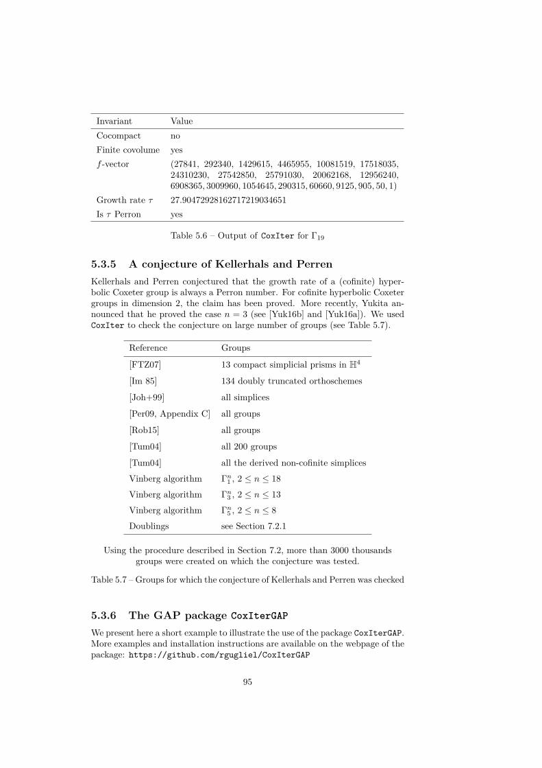
Invariant ValueCocompact noFinite covolume yesf -vector (27841, 292340, 1429615, 4465955, 10081519, 17518035,
24310230, 27542850, 25791030, 20062168, 12956240,6908365, 3009960, 1054645, 290315, 60660, 9125, 905, 50, 1)
Growth rate τ 27.90472928162717219034651Is τ Perron yes
Table 5.6 – Output of CoxIter for Γ19
5.3.5 A conjecture of Kellerhals and PerrenKellerhals and Perren conjectured that the growth rate of a (cofinite) hyper-bolic Coxeter group is always a Perron number. For cofinite hyperbolic Coxetergroups in dimension 2, the claim has been proved. More recently, Yukita an-nounced that he proved the case n = 3 (see [Yuk16b] and [Yuk16a]). We usedCoxIter to check the conjecture on large number of groups (see Table 5.7).
Reference Groups
[FTZ07] 13 compact simplicial prisms in H4
[Im 85] 134 doubly truncated orthoschemes
[Joh+99] all simplices
[Per09, Appendix C] all groups
[Rob15] all groups
[Tum04] all 200 groups
[Tum04] all the derived non-cofinite simplices
Vinberg algorithm Γn1 , 2 ≤ n ≤ 18
Vinberg algorithm Γn3 , 2 ≤ n ≤ 13
Vinberg algorithm Γn5 , 2 ≤ n ≤ 8
Doublings see Section 7.2.1
Using the procedure described in Section 7.2, more than 3000 thousandsgroups were created on which the conjecture was tested.
Table 5.7 – Groups for which the conjecture of Kellerhals and Perren was checked
5.3.6 The GAP package CoxIterGAP
We present here a short example to illustrate the use of the package CoxIterGAP.More examples and installation instructions are available on the webpage of thepackage: https://github.com/rgugliel/CoxIterGAP
95
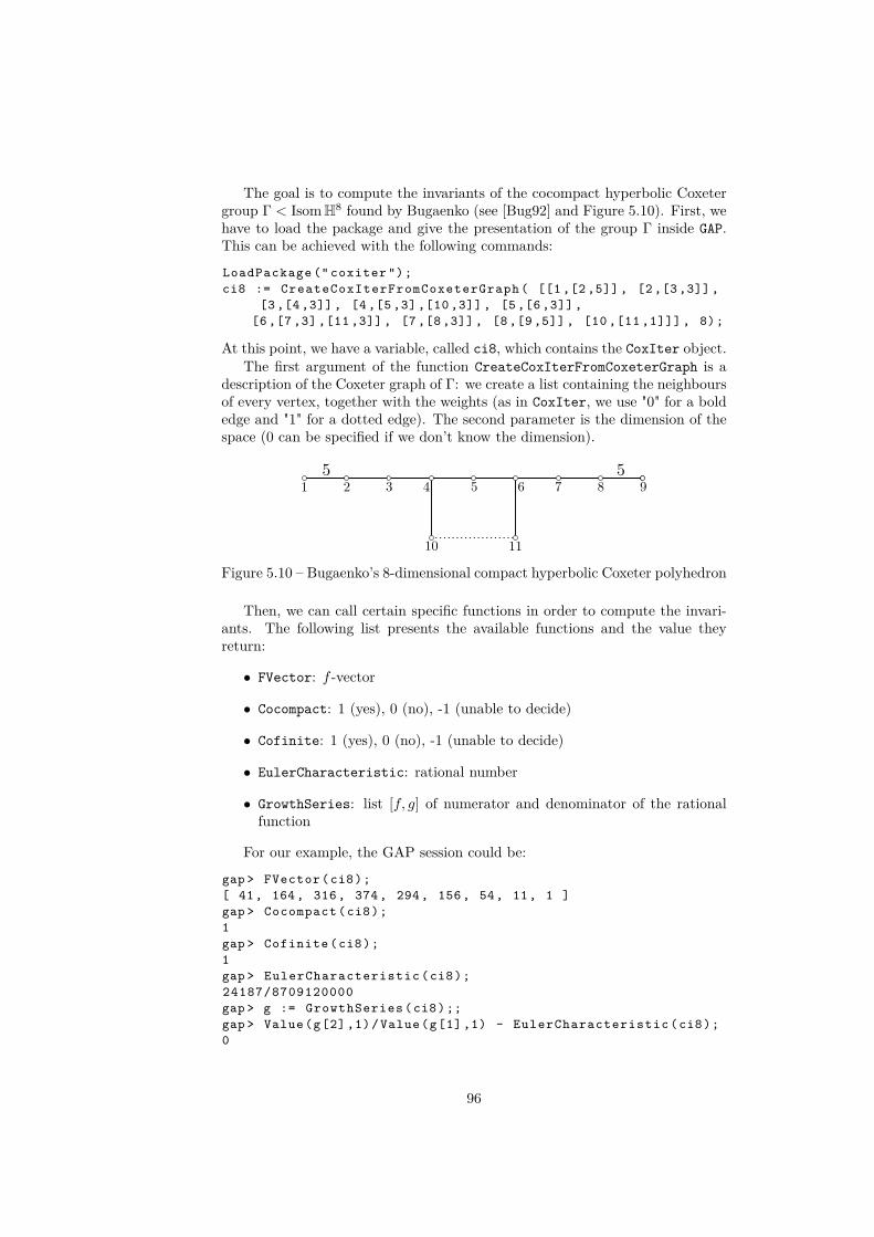
The goal is to compute the invariants of the cocompact hyperbolic Coxetergroup Γ < IsomH8 found by Bugaenko (see [Bug92] and Figure 5.10). First, wehave to load the package and give the presentation of the group Γ inside GAP.This can be achieved with the following commands:
LoadPackage (" coxiter ");ci8 := CreateCoxIterFromCoxeterGraph ( [[1 ,[2 ,5]] , [2 ,[3 ,3]] ,
[3 ,[4 ,3]] , [4 ,[5 ,3] ,[10 ,3]] , [5 ,[6 ,3]] ,[6 ,[7 ,3] ,[11 ,3]] , [7 ,[8 ,3]] , [8 ,[9 ,5]] , [10 ,[11 ,1]]] , 8);
At this point, we have a variable, called ci8, which contains the CoxIter object.The first argument of the function CreateCoxIterFromCoxeterGraph is a
description of the Coxeter graph of Γ: we create a list containing the neighboursof every vertex, together with the weights (as in CoxIter, we use "0" for a boldedge and "1" for a dotted edge). The second parameter is the dimension of thespace (0 can be specified if we don’t know the dimension).
Figure 5.10 – Bugaenko’s 8-dimensional compact hyperbolic Coxeter polyhedron
Then, we can call certain specific functions in order to compute the invari-ants. The following list presents the available functions and the value theyreturn:
• FVector: f -vector
• Cocompact: 1 (yes), 0 (no), -1 (unable to decide)
• Cofinite: 1 (yes), 0 (no), -1 (unable to decide)
• EulerCharacteristic: rational number
• GrowthSeries: list [f, g] of numerator and denominator of the rationalfunction
For our example, the GAP session could be:
gap > FVector (ci8);[ 41, 164 , 316, 374, 294, 156, 54, 11, 1 ]gap > Cocompact (ci8);1gap > Cofinite (ci8);1gap > EulerCharacteristic (ci8);24187/8709120000gap > g := GrowthSeries (ci8);;gap > Value(g[2] ,1)/Value(g[1] ,1) - EulerCharacteristic (ci8);0
96

5.4 Encoding a graphTo give a Coxeter graph to CoxIter, it is sufficient to create a text file todescribe the graph. The file contains the following:
• Number of vertices and dimensionThe first line contains the number of vertices of the graph and the dimen-sion n such that the associated polyhedron lives in Hn. Remark that thedimension is optional: it is needed only for the compactness and cofinite-ness tests and CoxIter will try to guess it if it is not given.
• Name of the verticesBy default, the vertices are labelled 1, 2, . . . , r. It is however possible tospecify other labels. In order to do this, the second line has to be of theform
vertices labels: label1 label2 label3 ...
Each label can contains letters, digits, -, _ but not space.
• Edges of the graphThen, we have to add one line to describe each edge of the graph. Thesyntax is the following:
vertex1 vertex2 weight
Remarks:
– 0 is used to specify the weight infinity and 1 is used to specify adotted edge.
– The weight 2 doesn’t have to be specified.
For example, the 2-dimensional hyperbolic Coxeter group whose graph isgiven in Figure 5.11 could be described for CoxIter in the two following equiv-alent ways:
4 21 2 12 3 43 4 1
4 2vertices labels: s1 s2 s3 ts1 s2 1s2 s3 4s3 t 1
Figure 5.11 – The group of units of the quadratic form 〈−6, 1, 1〉
Note that it is possible (although not mandatory) to indicate the weight ofa dotted line after a #. If all these weights are specified, then CoxIter willbe able to numerically compute the signature as well as improve some outputs.The example of Figure 5.11 then becomes:
4 21 2 1 # -sqrt(2)2 3 43 4 1 # -sqrt(3/2)
97
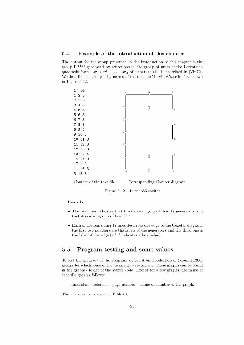
5.4.1 Example of the introduction of this chapterThe output for the group presented in the introduction of this chapter is thegroup Γ(14,1) generated by reflections in the group of units of the Lorentzianquadratic form −x2
0 + x21 + . . . + x2
14 of signature (14, 1) described in [Vin72].We describe the group Γ by means of the text file "14-vinb85.coxiter" as shownin Figure 5.12.
17 141 2 32 3 33 4 34 5 35 6 36 7 37 8 38 9 39 10 310 11 311 12 312 13 313 14 414 17 017 1 411 16 33 15 3
Content of the text file Corresponding Coxeter diagram
Figure 5.12 – 14-vinb85.coxiter
Remarks:
• The first line indicates that the Coxeter group Γ has 17 generators andthat it is a subgroup of IsomH14.
• Each of the remaining 17 lines describes one edge of the Coxeter diagram:the first two numbers are the labels of the generators and the third one isthe label of the edge (a "0" indicates a bold edge).
5.5 Program testing and some values
To test the accuracy of the program, we ran it on a collection of (around 1200)groups for which some of the invariants were known. These graphs can be foundin the graphs/ folder of the source code. Except for a few graphs, the name ofeach file goes as follows:
dimension− reference_page number− name or number of the graph.
The reference is as given in Table 5.8.
98
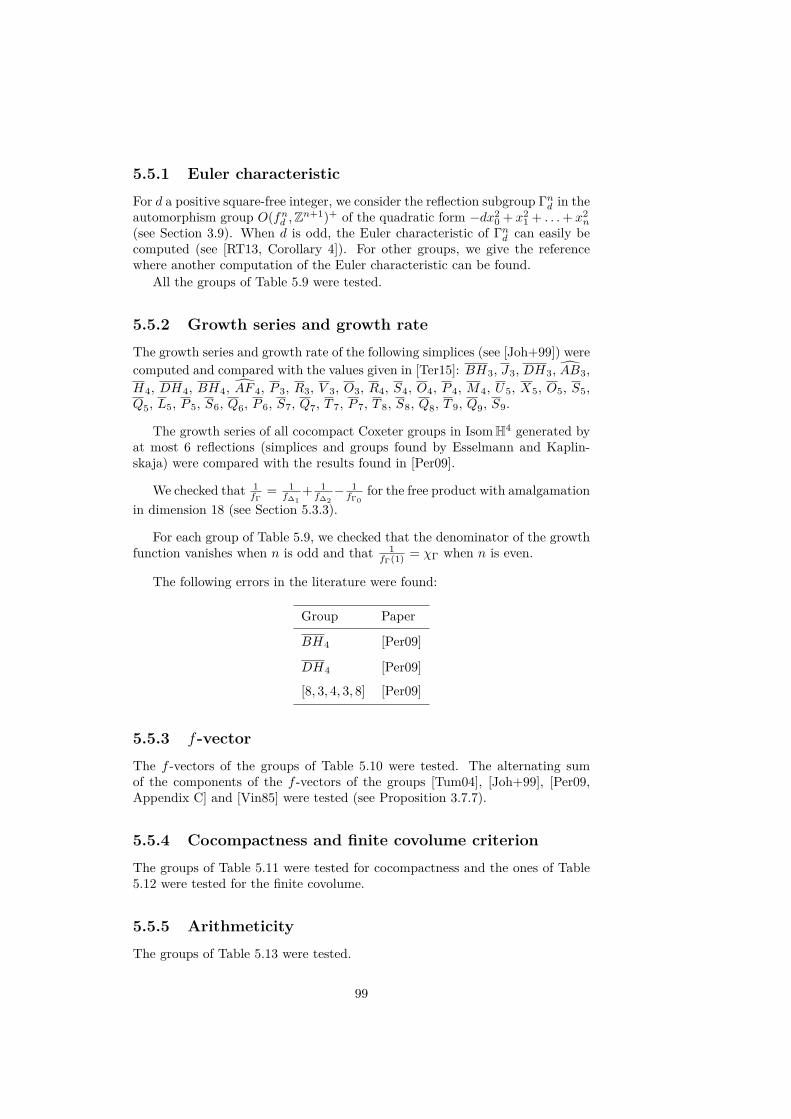
5.5.1 Euler characteristicFor d a positive square-free integer, we consider the reflection subgroup Γnd in theautomorphism group O(fnd ,Zn+1)+ of the quadratic form −dx2
0 + x21 + . . .+ x2
n
(see Section 3.9). When d is odd, the Euler characteristic of Γnd can easily becomputed (see [RT13, Corollary 4]). For other groups, we give the referencewhere another computation of the Euler characteristic can be found.
All the groups of Table 5.9 were tested.
5.5.2 Growth series and growth rateThe growth series and growth rate of the following simplices (see [Joh+99]) werecomputed and compared with the values given in [Ter15]: BH3, J3, DH3, AB3,H4, DH4, BH4, AF 4, P 3, R3, V 3, O3, R4, S4, O4, P 4, M4, U5, X5, O5, S5,Q5, L5, P 5, S6, Q6, P 6, S7, Q7, T 7, P 7, T 8, S8, Q8, T 9, Q9, S9.
The growth series of all cocompact Coxeter groups in IsomH4 generated byat most 6 reflections (simplices and groups found by Esselmann and Kaplin-skaja) were compared with the results found in [Per09].
We checked that 1fΓ
= 1f∆1
+ 1f∆2− 1fΓ0
for the free product with amalgamationin dimension 18 (see Section 5.3.3).
For each group of Table 5.9, we checked that the denominator of the growthfunction vanishes when n is odd and that 1
fΓ(1) = χΓ when n is even.
The following errors in the literature were found:
Group Paper
BH4 [Per09]
DH4 [Per09]
[8, 3, 4, 3, 8] [Per09]
5.5.3 f-vectorThe f -vectors of the groups of Table 5.10 were tested. The alternating sumof the components of the f -vectors of the groups [Tum04], [Joh+99], [Per09,Appendix C] and [Vin85] were tested (see Proposition 3.7.7).
5.5.4 Cocompactness and finite covolume criterionThe groups of Table 5.11 were tested for cocompactness and the ones of Table5.12 were tested for the finite covolume.
5.5.5 ArithmeticityThe groups of Table 5.13 were tested.
99

5.5.6 Some more complicated Coxeter graphsUsing groups mentioned in this section, we created more than 3000 thousandsgroups (small sequences of index two subgroups, as explained in Section 7.2)and these groups allowed us to test CoxIter and the conjecture of Kellerhalsand Perren on more complicated graphs (the number of nodes ranges from 7 to775).
100
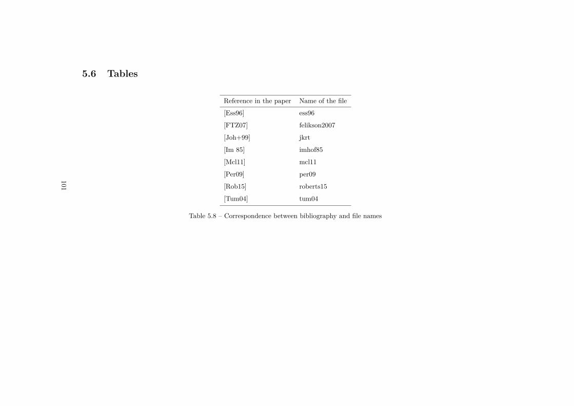
5.6 Tables
Reference in the paper Name of the file
[Ess96] ess96
[FTZ07] felikson2007
[Joh+99] jkrt
[Im 85] imhof85
[Mcl11] mcl11
[Per09] per09
[Rob15] roberts15
[Tum04] tum04
Table 5.8 – Correspondence between bibliography and file names
101
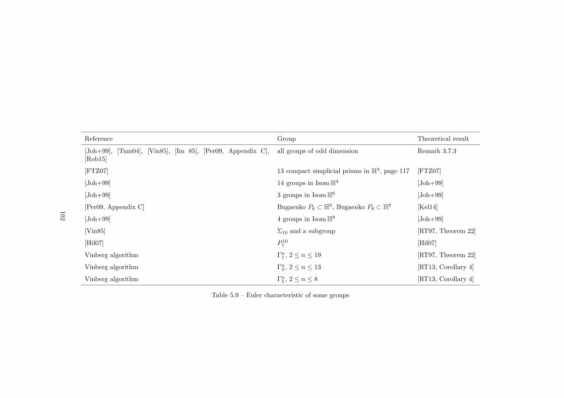
Reference Group Theoretical result
[Joh+99], [Tum04], [Vin85], [Im 85], [Per09, Appendix C],[Rob15]
all groups of odd dimension Remark 3.7.3
[FTZ07] 13 compact simplicial prisms in H4, page 117 [FTZ07]
[Joh+99] 14 groups in IsomH4 [Joh+99]
[Joh+99] 3 groups in IsomH6 [Joh+99]
[Per09, Appendix C] Bugaenko P6 ⊂ H6, Bugaenko P8 ⊂ H8 [Kel14]
[Joh+99] 4 groups in IsomH8 [Joh+99]
[Vin85] Σ10 and a subgroup [RT97, Theorem 22]
[Hil07] P 101 [Hil07]
Vinberg algorithm Γn1 , 2 ≤ n ≤ 19 [RT97, Theorem 22]
Vinberg algorithm Γn3 , 2 ≤ n ≤ 13 [RT13, Corollary 4]
Vinberg algorithm Γn5 , 2 ≤ n ≤ 8 [RT13, Corollary 4]
Table 5.9 – Euler characteristic of some groups
102

Group Theoretical result
all groups of [Joh+99] simplices
all pyramids in H3 of [Tum04] pyramids
Bugaenko P6 [Kel14]
Bugaenko P8 [Zeh09]
Birectified 5-simplex http://en.wikipedia.org/wiki/Rectified_5-simplexes
Table 5.10 – f -vector of some groups
103
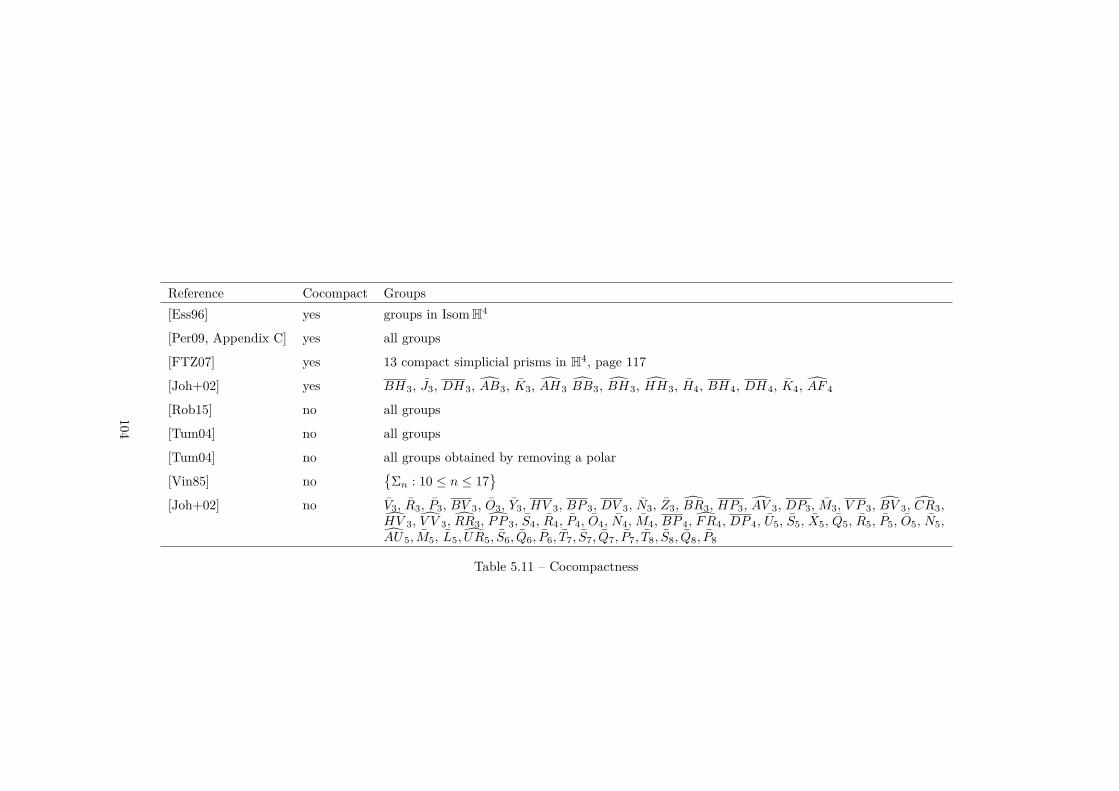
Reference Cocompact Groups[Ess96] yes groups in IsomH4
[Per09, Appendix C] yes all groups
[FTZ07] yes 13 compact simplicial prisms in H4, page 117
[Joh+02] yes BH3, J3, DH3, AB3, K3, AH3 BB3, BH3, HH3, H4, BH4, DH4, K4, AF 4
[Rob15] no all groups
[Tum04] no all groups
[Tum04] no all groups obtained by removing a polar
[Vin85] no
Σn : 10 ≤ n ≤ 17
[Joh+02] no V3, R3, P3, BV 3, O3, Y3, HV 3, BP 3, DV 3, N3, Z3, BR3, HP3, AV 3, DP3, M3, V P 3, BV 3, CR3,HV 3, V V 3, RR3, PP 3, S4, R4, P4, O4, N4, M4, BP 4, FR4, DP 4, U5, S5, X5, Q5, R5, P5, O5, N5,AU5, M5, L5, UR5, S6, Q6, P6, T7, S7, Q7, P7, T8, S8, Q8, P8
Table 5.11 – Cocompactness
104
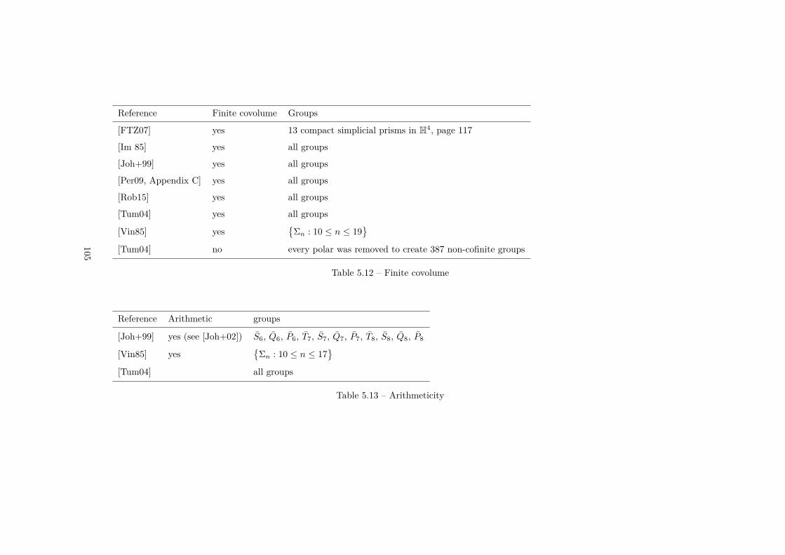
Reference Finite covolume Groups
[FTZ07] yes 13 compact simplicial prisms in H4, page 117
[Im 85] yes all groups
[Joh+99] yes all groups
[Per09, Appendix C] yes all groups
[Rob15] yes all groups
[Tum04] yes all groups
[Vin85] yes
Σn : 10 ≤ n ≤ 19
[Tum04] no every polar was removed to create 387 non-cofinite groups
Table 5.12 – Finite covolume
Reference Arithmetic groups
[Joh+99] yes (see [Joh+02]) S6, Q6, P6, T7, S7, Q7, P7, T8, S8, Q8, P8
[Vin85] yes
Σn : 10 ≤ n ≤ 17
[Tum04] all groups
Table 5.13 – Arithmeticity
105

106

CHAPTER 6The Vinberg algorithm and AlVin
In this chapter, we present Vinberg’s algorithm and study it from an algorithmicpoint of view. The goal is to explain the key ingredients which are used in AlVin(for Algorithm of Vinberg), a C++ program which we design to carry on thecomputations of the algorithm for diagonal quadratic forms with K = Q (non-cocompact case) and with K = Q[
√d],Q
[cos 2π
7](cocompact cases). Since we
also want the program to be able in some cases to decide the non-reflectivity ofa quadratic form, we present two methods for achieving this goal.
In the first section, we give an overview of the algorithm and present anexhaustive list of computations done with the algorithms by other authors. Inthe second section, we present in details the theoretical background needed tounderstand the algorithm.
In sections 6.3 to 6.5, we give more information about the implementationsinto the computer program AlVin: we explain how the solutions of the equationscan be parametrized for each of our three fields. Finally, we show in details howto use AlVin and we present some results: new polyhedra (compacts and non-compacts, in dimensions 2 to 9), classification of diagonal quadratic form ofsignature (3, 1) with small coefficients, non-reflectivity of some forms, etc.
The program, together with its documentation, can be found here: https://github.com/rgugliel/AlVin
6.1 IntroductionIn [Vin72], Vinberg presented an algorithm to create hyperbolic Coxeter groups1
in the arithmetic context. The starting point is a totally real number field K,together with an admissible (we will be more precise below) quadratic form f ofsignature (n, 1) which is given, with respect to some basis v0, . . . , vn of Kn+1
byf(x0, . . . , xn) =
∑i,j
ai,j · xi xj ,
1Strictly speaking, the algorithm is more general: its goal is to find, for any discretesubgroup Θ of IsomHn, the maximal subgroup of Θ generated by reflections. However, if wedon’t take Θ to be the group of units of some quadratic form, then finding the reflections ismuch more difficult.
107

where ai,j ∈ OK . We also consider a lattice L in Kn+1 (i.e. L is the OK-spanof n+ 1 linearly independent vectors, where OK denotes the ring of integers ofK).
We now consider the group Θf,L of isomorphisms of the quadratic form f ,which preserves the lattice L and the two sheets of the hyperboloid definedby f (see Section 3.9.1) and we know that Θf,L is a discrete group of finitecovolume (again, see Section 3.9.1). We recall from Section 3.9, that we havethe decomposition Θf,L = Γf,LoH, as a semi-direct product, where Γf,L is thesubgroup of Θf,L generated by all the reflections in Θf,L and H is a subgroupof the symmetry group of a cell P of Γf,L. Vinberg’s algorithm describes a wayto find successively the normal vectors of the polyhedron2 P (and of course apresentation of the group Γf,L):
1. First, we start with a set of n vectors V = e1, . . . , en whose correspond-ing hyperplanes go through a specified point (for example the point p0corresponding to the vector v0, which is chosen such that f(v0) < 0).These vectors give rise to a polyhedron
⋂ei∈V H
−ei of infinite volume.
2. We look for a vector en+1 which stabilizes the lattice spanned by thev0, . . . , vn and which satisfies some relations with the previous found vec-tors (again, we will be more precise below) and we add en+1 to our col-lection V. If the polyhedron
⋂ei∈V H
−ei is of finite volume, we stop.
3. As long as the polyhedron defined by the vectors in V is not of finitevolume, we continue to look for another vector and we add it to the col-lection V.
At this point, it is worth to mention that we cannot say a priori if Γf,L is offinite index in Θf,L or, what is equivalent, if the covolume of Γf,L is finite (inthis setting, we say that the form f is reflective). In terms of the algorithm itmeans the following: if the polyhedron
⋂ei∈V H
−ei is not of finite volume, there
is no way to know whether we have to continue to add vectors to the list V orwhether P is not finite sided. If the algorithm stops, then we have found a cellP of the group Γf,L (see [Vin72, Proposition 4]).
Remark 6.1.1Although the choice of the base point p0 (corresponding to the vector v0) is ir-relevant, considering only diagonal quadratic forms (and to the lattice spannedover the ring of integers by a diagonalizing basis) is a limitation. Indeed, evenif every quadratic form can be transformed into a diagonal form over its defin-ing field, it is not true that we can do the same with a transformation withcoefficients in the ring of integers. For example, the 8 dimensional compactCoxeter polyhedron found by Bugaenko (see [Bug92]) is based on the lattice[−(√
5 + 1)]⊕E8, which does not correspond to a diagonal quadratic form overOQ[√
5].
Remark 6.1.2In this work, we will always take f to be a diagonal quadratic form with respect
2The word polyhedron is used here in a wide sense since we do not know whether it isfinite sided or not and whether if it has finite volume. We will allow this generalization forthe whole chapter.
108
to a basis v0, . . . , vn and take L to be the lattice spanned over OK by thevi (this choice regarding the lattice is not a restriction, as indicated in Remark3.9.2). In this setting, we will write Θf for Θf,L and Γf for Γf,L. Moreover, thegroup Θf is then called the group of units of f and we will sometimes refer to Γf(respectively P ) as the reflection group (respectively the polyhedron) associatedto f .
Before our work, the algorithm has mostly been used for diagonal quadraticforms of the type fnα = 〈−α, 1, . . . , 1〉 (see Section 6.6 for more complicated andnew examples):
• α = 1 (standard Lorentzian form)In [Vin72], Vinberg found groups for 2 ≤ n ≤ 17. Together with Kaplin-skaya, they applied the algorithm for n = 18, 19 and proved that the formfn1 is not reflective if n > 19 (see [KV78]).
• α = 2The form is reflective for 2 ≤ n ≤ 14 (see [Vin72]).
• α = 3McLeod studied in [Mcl11] the form for α = 3 and showed that it isreflective for 2 ≤ n ≤ 13. In his thesis (see [Mcl13]) he also performedsome other applications of the algorithm, with some errors (see Remark6.2.3 and sections 6.8.1.3 and 6.8.3.3).
• α = 5The form is reflective for 2 ≤ n ≤ 8 (see [Mar12]).
• α = 7, 11, 13, 17, 19, 23Mark showed in [Mar12] that the forms with α = 7, 17 are reflective onlyif n = 2, 3; the forms α = 13, 19, 23 are reflective only if n = 2 and theform with α = 11 is reflective if n = 2, 3, 4.
• α = 1+√
52
The form is reflective for 2 ≤ n ≤ 7 (see [Bug84]).
• α = 1 +√
2The form is reflective for 2 ≤ n ≤ 6 (see [Bug90]).
• α = 2 cos 2π7
The form is reflective for n = 2, 3, 4 (see [Bug92]).
In [Gro08], Grosek applied the algorithm to the forms 〈−1, 1,m〉, withm = 1,2, . . . , 14, 16, 18, 20 and to the forms 〈−1,m,m〉 for m = 1, 2, . . . , 12.
In [Sch89], R. Scharlau classified all reflective quadratic forms of signature(3, 1) such that the group Γf is non-cocompact (meaning that f is defined overZ and is isotropic, as indicated in Remark 3.9.2)3. There are 49 of such forms.Whenever it is possible, we will give the corresponding diagonal quadratic form(see Section 6.8.1.1).
3Note that the forms given by Scharlau are not in diagonal form.
109

6.2 Theoretical partLet K be a totally real number field such that the ring of integers OK of K is aunique factorization domain4. Let V be aK-vector space of dimension n+1 withbasis v0, . . . , vn and let L be the lattice generated by v0, . . . , vn, that is L isthe OK-span of the basis vi. As in Section 3.9, we consider a quadratic formf of signature (n, 1) which is diagonal with respect to the basis v0, . . . , vn:f = 〈−α0, α1, . . . , αn〉, where each αi ∈ OK is positive and does not have anysquare factor. We suppose moreover that f is admissible, which means that fσis positive definite for every non-identity Galois embedding σ : K −→ R. Inthis setting, we will write Θf for the group O(f, L). Finally, we suppose thatif 1 ≤ i < j ≤ n are such that αi 6= αj then the ratio αi/αj is not the squareof an invertible element in OK : in other words, we fix once and for all onerepresentative of each class of the quotient OK/(O∗K)2.
Given such a quadratic form f , we also consider its associated bilinear form
(x, y) := 12(f(x+ y)− f(x)− f(y)
)= −α0 · x0y0 +
n∑i=1
αi · xiyi,
where the xi (respectively yi) denote the components of x (respectively y) withrespect to the basis v0, . . . , vn. Any vector e gives rise to a reflection
Re : V −→ V
x 7−→ x− 2(x, e)(e, e) e.
By a root of f , or simply a root, we mean a vector e in V such that thereflection Re with respect to the hyperplane He orthogonal to e preserves thelattice generated by v0, . . . , vn. If e is such a root, then we can suppose that thecoefficients k0, . . . , kn of e with respect to the basis v0, . . . , vn lie in OK anddon’t have any common factor. Indeed, since K is the field of fractions of OK ,each component ki can be written ai
bi. Then, the vector m · e, where m is the
least common multiple b0, b1, . . . , bn, which exists since OK is supposed to bea unique factorization domain, satisfies Rm·e = Re and has coefficients in OK .Moreover, if the gcd g of the ki is not 1, then can we can consider e′ = e
g inorder to get an irreducible, or primitive, root.
Finally, notice that preservation of the lattice is equivalent to the crystallo-graphic condition
(e, e) | 2αi ki, ∀ 0 ≤ i ≤ n. (6.1)
Indeed, applying Re to the basis vi, we see that the preservation of the latticeis equivalent to
−2 αi ki(e, e)kj , ∀i 6= j.
Since the the root e is supposed to be primitive (i.e. the ki don’t have anycommon factor), then we must have (e, e) | 2αi ki for every i, as required.
4This assumption, although not theoretically necessary, is needed for computations in thering of the integers OK
110
Remark 6.2.1When working with the algorithm, we will use the vector space model Hn in-duced by the quadratic form f : we consider the cone Cf = x ∈ Kn+1 ⊗ R :f(x) < 0 and its two connected components C±f and we let Hn be C+
f /R∗.
6.2.1 Description of the algorithmWe fix an admissible quadratic form f and we let Θf = O(f, L) and Γf as above.
The first step is to fix a point p0 ∈ Hn. For the sake of simplicity, we willalways consider p0 corresponding to the basis vector v0. The subgroup Γ0 ofthe discrete group Γf generated by the reflections which fix p0 is a finite groupof rank k at most n. We consider one cell P0 of Γ0 (it is a polyhedral coneemanating from p0) and its normal vectors e1, . . . , en (see Section 6.2.3 aboutfinding these vectors and the reason why k = n when p0 corresponds to v0).Among all the cells of Γf , we choose the unique cell P which is the same as P0in a sufficiently small neighbourhood of p0.
At this point, we have P0 =⋂ni=1H
−ei and we want to construct a (hopefully
finite) sequence e1, . . . , en, en+1, . . . such that Rei ∈ Γf and P :=⋂iH−ei has
finite volume. We proceed inductively. Suppose we have the finite sequencee1, . . . , er, r ≥ n. Among all the vectors e such that Re ∈ Γf , we choose er+1such that:
• (er+1, ei) ≤ 0 for all 1 ≤ i ≤ r;
• the distance d(p0, Her+1) is minimal.
Moreover, we choose the orientation of er+1 such that p0 ∈ H−er+1(i.e. we want
p0 to lie inside P ). As long as the polyhedron given by the ei is of infinitevolume, we continue to look for new vectors5.
A result of Vinberg (see [Vin72, Proposition 4]) ensures that the vectors eiindeed give rise to the required polyhedron P which is a cell of the group Γf .
Remarks 6.2.2 • The distance d(p0, Her+1) is given by
sinh2 d(p0, Her+1
)= − (er+1, v0)2
(er+1, er+1) · (v0, v0) .
Hence, since (v0, v0) = −α0 < 0, minimizing this distance is equivalentto minimizing the value (er+1,v0)2
(er+1,er+1) . With our assumption, this in turn
reduces to minimizing the value k20
(er+1,er+1) , where k0 is the first componentof er+1.
• The condition p0 ∈ H−er+1is equivalent to (v0, er+1) ≤ 0.
6.2.2 Possible values for (e, e)Let e be a root and suppose that (e, e) ∈ OK is not invertible. Let π ∈ OKbe a prime factor of (e, e). Since the coefficients of e don’t have any common
5As we will see later, the more we go on, the more complicated the computations become.
111
factor by assumption, there exists 0 ≤ j ≤ n such that π | 2 · αj . If we denoteby P the set of prime elements of OK which divide at least one coefficient ofthe quadratic form f and by ρ1, . . . , ρk ∈ OK the prime factors of 2, then wesee that (e, e) can be written as follows:
(e, e) = u · ρ0,11 · . . . · ρ0,1
k ·r∏i=1
πi, πi ∈ P, u ∈ O∗K , (6.2)
where x0,1 means x0 or x1. Moreover, since the coefficients of f don’t have anysquare factor, we can suppose that that the πi are distinct. Finally, since f isadmissible, all the conjugates of (e, e) must be positive.
Finally, equation (6.2) implies that in order to find the possible norms (e, e)it is sufficient to find the primes dividing the coefficients of the quadratic form,the decomposition of 2 and the invertible elements of OK (see Theorem 2.2.1)and to list all the possible products, omitting the ones which have some negativeconjugate.Remark 6.2.3Our description of the possible values of (e, e) is in contradiction with [Mcl13,Lemma 3.1.5], where only a smaller number of values is considered. This willlead us to some differences in the set of normal vectors of certain polytopes.
6.2.3 First set of vectorsFirst, we consider the group Γ0 generated by reflections in Γ stabilizing p0. Ife is a root such that Re ∈ Γ0, then the angle between e and any vi is 0, π2 or π
4(see [Bug92, Lemma 2.2]). Now, if there exists 1 ≤ i ≤ n such that ](e, vi) = π
4 ,then there exists precisely another j 6= i such that ](e, vj) = π
4 . Hence, we have
e = kivi + kjvj .
The crystallographic condition (6.1) implies that ki, kj ∈ O∗K and thus thequotient αi
αjis a square in O∗K . By hypothesis on f , we thus have αi = αj and
finally ki = ±kj . Therefore, the reflections in Γ0 are precisely the following
R±vi , 1 ≤ i ≤ n, R±vi±vj , 1 ≤ i < j ≤ n, when αi = αj .
Suppose now that f = 〈−α0, α′1, . . . , α
′1, . . . , α
′r, . . . , α
′r〉, where the α′i are dis-
tinct, and that the coefficient α′i appears ni times. We can now use the well-known classification of irreducible finite Coxeter groups to see that
Γ0 ∼=r∏i=1
Cni ,
with the convention that C1 = A1 and C2 = G42 (see also Figure 3.1, page 36).
Therefore, we form the initial set of vectors as follows:
− v1 + v2, . . . ,−vn1−1 + vn1 ,−vn1 n1 vectors− vn1+1 + vn1+2, . . . ,−vn1+n2−1 + vn1+n2 ,−vn1+n2 n2 vectors
......
− vn1+...+nr−1+1 + vn1+...+nr−1+2, . . . ,−vn−1 + vn,−vn nr vectors
Hence, we have n1 + . . .+ nr = n vectors and if we label them e1, . . . , en, thenwe have P0 =
⋂ni=1H
−ei , as required.
112
6.2.4 Solving the norm equationWe want to find another root e = (k0, . . . , kn). Since the first component andthe norm are prescribed by the fraction (e,v0)2
(e,e) which we have to minimize, weonly need to find the n remaining components. We do that inductively and bya "brute-force" search: if the components k0, . . . , kj−1 are chosen, then we have
∑i≥j
αik2i = (e, e) + α0k
20 −
j−1∑i=1
αik2i .
If σ : K −→ R denotes any non-trivial Galois embedding, then the fact that fσis positive definite implies
σ
αjk2j +
∑i>j
αik2i
= σ
((e, e) + α0k
20 −
j−1∑i=1
αik2i
)≥ 0,
which easily yields the condition
|σ(kj)| ≤
√√√√σ
((e, e) + α0k2
0 −∑j−1i=1 αik
2i
αj
).
If we let Sj = (e, e) + α0k20 −
∑j−1i=1 αik
2i , then we get the system
0 ≤ kj ≤√
Sjαj
−√σ(Sjαj
)≤ σ(kj) ≤
√σ(Sjαj
), ∀σ 6= id .
(6.3)
For each possible value of kj , we check if the crystallographic condition (6.1) issatisfied, and if it is the case, we try to find possible values for kj+1.
Remark 6.2.4 (i) Let e′ = (k′0, . . . , k′n) be a root of the quadratic form f .Since the coefficients α1, . . . , αn of the quadratic form are positive, the"partial product" between e′ and the candidate e
O∗K −→ O∗K
kj+1 7−→j+1∑i=0
αik′iki
is increasing. Therefore, the condition (e, ei) ≤ 0 for each found root eigives a stronger condition in the first inequality of the system (6.3).
(ii) When k = Q, the crystallographic condition (6.1) allows us to replace 0by (e,e)
gcd(
(e,e),2αj) in the first inequality of the system (6.3).
6.2.5 A first example
Let f = 〈−1, 2, 6, 6〉. Using Section 6.2.3, we see that Γ0 ∼= A1 ×G(4)2 , and that
the normal vectors of P0 are
e1 = (0,−1, 0, 0), e2 = (0, 0,−1, 1), e3 = (0, 0, 0,−1).
113
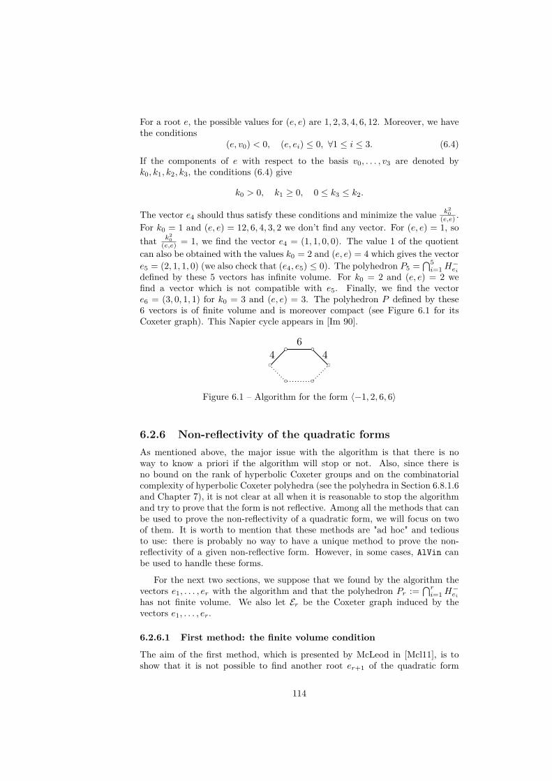
For a root e, the possible values for (e, e) are 1, 2, 3, 4, 6, 12. Moreover, we havethe conditions
(e, v0) < 0, (e, ei) ≤ 0, ∀1 ≤ i ≤ 3. (6.4)
If the components of e with respect to the basis v0, . . . , v3 are denoted byk0, k1, k2, k3, the conditions (6.4) give
k0 > 0, k1 ≥ 0, 0 ≤ k3 ≤ k2.
The vector e4 should thus satisfy these conditions and minimize the value k20
(e,e) .For k0 = 1 and (e, e) = 12, 6, 4, 3, 2 we don’t find any vector. For (e, e) = 1, sothat k2
0(e,e) = 1, we find the vector e4 = (1, 1, 0, 0). The value 1 of the quotient
can also be obtained with the values k0 = 2 and (e, e) = 4 which gives the vectore5 = (2, 1, 1, 0) (we also check that (e4, e5) ≤ 0). The polyhedron P5 =
⋂5i=1H
−ei
defined by these 5 vectors has infinite volume. For k0 = 2 and (e, e) = 2 wefind a vector which is not compatible with e5. Finally, we find the vectore6 = (3, 0, 1, 1) for k0 = 3 and (e, e) = 3. The polyhedron P defined by these6 vectors is of finite volume and is moreover compact (see Figure 6.1 for itsCoxeter graph). This Napier cycle appears in [Im 90].
Figure 6.1 – Algorithm for the form 〈−1, 2, 6, 6〉
6.2.6 Non-reflectivity of the quadratic formsAs mentioned above, the major issue with the algorithm is that there is noway to know a priori if the algorithm will stop or not. Also, since there isno bound on the rank of hyperbolic Coxeter groups and on the combinatorialcomplexity of hyperbolic Coxeter polyhedra (see the polyhedra in Section 6.8.1.6and Chapter 7), it is not clear at all when it is reasonable to stop the algorithmand try to prove that the form is not reflective. Among all the methods that canbe used to prove the non-reflectivity of a quadratic form, we will focus on twoof them. It is worth to mention that these methods are "ad hoc" and tediousto use: there is probably no way to have a unique method to prove the non-reflectivity of a given non-reflective form. However, in some cases, AlVin canbe used to handle these forms.
For the next two sections, we suppose that we found by the algorithm thevectors e1, . . . , er with the algorithm and that the polyhedron Pr :=
⋂ri=1H
−ei
has not finite volume. We also let Er be the Coxeter graph induced by thevectors e1, . . . , er.
6.2.6.1 First method: the finite volume condition
The aim of the first method, which is presented by McLeod in [Mcl11], is toshow that it is not possible to find another root er+1 of the quadratic form
114
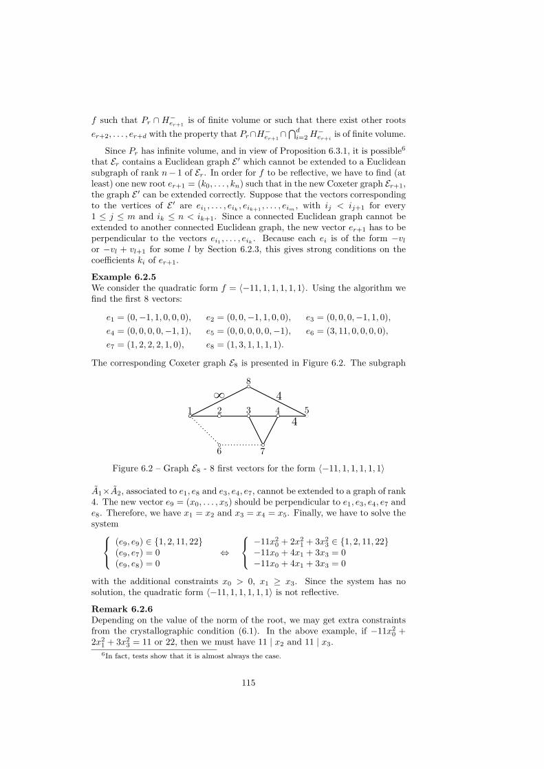
f such that Pr ∩H−er+1is of finite volume or such that there exist other roots
er+2, . . . , er+d with the property that Pr∩H−er+1∩⋂di=2H
−er+i is of finite volume.
Since Pr has infinite volume, and in view of Proposition 6.3.1, it is possible6
that Er contains a Euclidean graph E ′ which cannot be extended to a Euclideansubgraph of rank n− 1 of Er. In order for f to be reflective, we have to find (atleast) one new root er+1 = (k0, . . . , kn) such that in the new Coxeter graph Er+1,the graph E ′ can be extended correctly. Suppose that the vectors correspondingto the vertices of E ′ are ei1 , . . . , eik , eik+1 , . . . , eim , with ij < ij+1 for every1 ≤ j ≤ m and ik ≤ n < ik+1. Since a connected Euclidean graph cannot beextended to another connected Euclidean graph, the new vector er+1 has to beperpendicular to the vectors ei1 , . . . , eik . Because each ei is of the form −vlor −vl + vl+1 for some l by Section 6.2.3, this gives strong conditions on thecoefficients ki of er+1.
Example 6.2.5We consider the quadratic form f = 〈−11, 1, 1, 1, 1, 1〉. Using the algorithm wefind the first 8 vectors:
e1 = (0,−1, 1, 0, 0, 0), e2 = (0, 0,−1, 1, 0, 0), e3 = (0, 0, 0,−1, 1, 0),e4 = (0, 0, 0, 0,−1, 1), e5 = (0, 0, 0, 0, 0,−1), e6 = (3, 11, 0, 0, 0, 0),e7 = (1, 2, 2, 2, 1, 0), e8 = (1, 3, 1, 1, 1, 1).
The corresponding Coxeter graph E8 is presented in Figure 6.2. The subgraph
Figure 6.2 – Graph E8 - 8 first vectors for the form 〈−11, 1, 1, 1, 1, 1〉
A1×A2, associated to e1, e8 and e3, e4, e7, cannot be extended to a graph of rank4. The new vector e9 = (x0, . . . , x5) should be perpendicular to e1, e3, e4, e7 ande8. Therefore, we have x1 = x2 and x3 = x4 = x5. Finally, we have to solve thesystem (e9, e9) ∈ 1, 2, 11, 22
(e9, e7) = 0(e9, e8) = 0
⇔
−11x20 + 2x2
1 + 3x23 ∈ 1, 2, 11, 22
−11x0 + 4x1 + 3x3 = 0−11x0 + 4x1 + 3x3 = 0
with the additional constraints x0 > 0, x1 ≥ x3. Since the system has nosolution, the quadratic form 〈−11, 1, 1, 1, 1, 1〉 is not reflective.
Remark 6.2.6Depending on the value of the norm of the root, we may get extra constraintsfrom the crystallographic condition (6.1). In the above example, if −11x2
0 +2x2
1 + 3x23 = 11 or 22, then we must have 11 | x2 and 11 | x3.
6In fact, tests show that it is almost always the case.
115

Remark 6.2.7This first approach only works well when working over Q: for other fields, theresolution of the system of equations is quite difficult. Moreover, programs suchas Mathematica R© don’t handle equations solving in number fields. One canwrite every element in a integral basis and write a system with more equationsbut then the computations become too complicated.
6.2.6.2 Second method: symmetries of the polyhedron
Recall that we have the decomposition Θf = Γf oH, where H is a subgroup ofthe symmetry group symP of the fundamental polyhedron P . Here, we will trydirectly to show that P is not finite sided by showing that its symmetry groupis infinite. The steps are the following:
1. Create symmetries η1, . . . , ηm of Pr which extend to integral symmetriesof P (see Lemma 6.2.8).
2. Show that the group ∆ := 〈η1, . . . , ηm〉 ≤ symP has no fixed point in Hn(see lemmas 6.2.10 and 6.2.11). Usually, two or three involutions will besufficient.
We will provide an example of this method in Section 6.6.5.
Lemma 6.2.8 (See also [Bug92, Lemma 3.3])Let G be a subgraph of the Coxeter graph of P , such that:
• The R-span of the vectors corresponding to the vertices of G has dimensionn+ 1.
• The graph G contains a spherical or Euclidean subgraph of maximal rank.
Then, any symmetry of G extends to a symmetry of P .
Remark 6.2.9In contrast to what the original lemma [Bug92, Lemma 3.3] says, the abovelemma only gives us a linear transformation of the space which preserves P .We still have to check that this involution preserves the quadratic form and thelattice spanned over OK by the canonical basis.
Lemma 6.2.10 (See [Bug92, Lemma 3.1])Let H be a discrete subgroup of IsomHn. Then, H is infinite if and only if thereexists a subgroup ∆ of H with Fix(∆) ∩ Hn = ∅, where Fix(∆) denotes the setof vectors fixed by every transformation on ∆.
Lemma 6.2.11 (See [Bug92, Lemma 3.2])Let η be an involutive transformation of an arbitrary real vector space V . Then,Fix η is generated by the vectors wi + η(wi), where wi is a R-basis of V .
Remark 6.2.12This method becomes more difficult to apply when the dimension of Hn in-creases because we have to find symmetric subgraphs with more and more ver-tices. Also, when the set of possible values for the norm of a root (which growsexponentially with the number of prime number dividing at least one coefficientof the quadratic form) is big, many symmetries of subgraphs do not preserve the
116

quadratic form. In both cases, it is necessary to compute more normal vectorsbefore trying this method. However, one advantage of this second approachcompared to the first one is to be independent7 of the base field K.
6.3 Towards the implementations
6.3.1 Global description of the implementation of the al-gorithm
Here are the main steps of the implementation of the algorithm for a givenquadratic form:
• We check that the quadratic form is admissible, has appropriate signatureand satisfies the condition on the ratios of its coefficients (see Section 6.2).
• We find a first set of n vectors, corresponding to roots of the lattice whosereflections generate the stabilizer Γ0 of v0 (see Section 6.2.3).
• We find the possible values for the norm of a root e (see Section 6.2.2).
• For given integersm < M we find all the possible fractionsm < k0(e,e) ≤M ,
where e = (k0, . . . , kn) is a root. We start with m = 0, M = 1 and wecontinue until the algorithm terminates (or when the maximal number ofvectors is achieved). We choose the fraction which has minimal value.
• For each fraction k20
(e,e) we try to find the remaining components k1, . . . , knof the root e. If we succeed, we add the vector e to the list and we checkif the polyhedron which is bounded by the hyperplanes perpendicular tothe vectors is of finite volume. If it is not the case, we try to find anotherroot from the next fraction.
6.3.2 Couples (k0, (e, e))Let m < M be two positive integers and let e = (k0, . . . , kn) and ε = (e, e). Wewant to determine all the fractions such that m <
k20ε ≤M . Since the quadratic
form fσ is positive definite for all non-trivial Galois embeddings σ : K −→ R,we have σ
(ε+ α0 · k0
2) > 0, with σ(α0) < 0, which gives the equations m · ε < k02 ≤M · ε
|σ(k0)| ≤√σ(
ε−α0
), ∀σ 6= id .
(6.5)
We will describe the solutions of this system when K = Q[√d] and K =
Q[cos 2π7 ] (see sections 6.5.2.3 and 6.5.3.3).
7This is not completely true since arithmetic computations in Q[cos 2π7 ] and Q[
√d] are
slower than in Q but the difference is acceptable.
117

6.3.3 Some optimizationsMost of the computation time is dedicated to one of the two following tasks:
1. Solving the norm equation.
2. Once a candidate has been found, checking whether the polyhedron is offinite volume.
6.3.3.1 Testing the volume finiteness
Besides the finite volume criterion (see Proposition 3.8.4), we have a partialcriterion from [Vin72, Proposition 1].
Proposition 6.3.1Let Γ < IsomHn be a Coxeter group and let G be the Coxeter graph of Γ. IfΓ is of finite covolume, then for each Euclidean subgraph E of G there exists aEuclidean subgraph E ′ of G of rank n−1 (see Definition 3.5.4) such that E ⊂ E ′.
If the condition of the Proposition 6.3.1 is satisfied, then it is possible thatΓ is of finite covolume. Since the number of Euclidean subgraphs is usuallymuch smaller than the number of spherical subgraphs, the test is faster thanthe complete criterion (more than 10000 faster for big graphs). If the partialtest succeeds, then we try again with the complete test.
6.4 General information about the programThe program AlVin is written in C++ and is free/open source. More precisely, itis published under a free license, the GPLv3 (the GNU General Public Licensev3) and can be used freely in various projects8. AlVin and its documentation (tobuild and use the program) is available on the website https://alvin.rgug.chand on GitHub: https://github.com/rgugliel/AlVin
6.4.1 External libraries usedAlVin requires the following external libraries:
CoxIter It is used as a library to check at each step if the polyhedron is of finitevolume or not. When the form is reflective, we use CoxIter to computethe invariants of the final polyhedron.
Eigen It is a C++ template library for linear algebra which is used for the non-reflective test.
Gaol This library is used to perform interval arithmetic.
GMP (or GNU Multiple Precision Arithmetic Library) is a free library forarbitrary precision arithmetic with integers.
8More information about the license can be found here: https://www.gnu.org/licenses/gpl.html A short guide is also available here: https://www.gnu.org/licenses/quick-guide-gplv3.html
118
igraph It is a C/C++ package designed to manipulate graphs and do networkanalysis used for the non-reflective test.
OpenMP Via CoxIter and for the non-reflective test.
PARI We use the C library PARI to factor the minimal polynomial of 2 cos 2π7
over Fp[x]. This library is also used through CoxIter to compute thegrowth rate of the final Coxeter group.
PCRE The PCRE library (PCRE - Perl Compatible Regular Expressions) isused to parse the user input.
6.4.2 Design descriptionWe briefly explain the main steps of the working flow of AlVin.
• Reading the parametersWhen the program is launched, it first lists all the given parameters (thefile to read and the options for the computations). This is done in theApp::bReadMainParameters function.
• First tests and initializationsWe test that the form is admissible, remove the square factors of the coef-ficients and check whether the gcd of the coefficients is invertible. Then,we compute the possible values for the norm of a root (AlVin::AlVin,AlVin::initializations and AlVin::findPossibleNorms2).
• First set of vectorsWe list the first n vectors, as explained in Section 6.2.3 (see functionAlVin::findFirstVectors).
• Computing the vectorsWe go through pairs (k0, (e, e)) by increasing value of k2
0(e,e) (AlVin::Run).
Once a vector is found, we check whether the polyhedron has finite volumeor not. We continue as long as the polyhedron does not have finite volumeor the number of vectors is less than the value "-maxv".
• Non-reflective testIf the algorithm did not succeed and if it was specified in the parameters,we try to determine if the form is not reflective (InfiniteNSymetries).
• Displaying final informationFinally, we display the information about the execution.
6.5 ImplementationsIn this section, we provide some details about computations in the differentimplementations of the algorithm. Mostly, this consists of the following:
• decompositions into prime numbers;
• parametrization of the solutions of systems (6.3) and (6.5) on pages 113and 117.
119
6.5.1 Rational integers6.5.1.1 Operations
For a real number x ∈ R, we have the respective functions floor(x) and ceil(x)which return respectively the largest integer not greater than x and smallestinteger not less than x.For a positive real number x, we define the integral square root SQRTinf(x)of x and the supremal integral square root SQRTsup(x) of x to be the integerssuch that
SQRTinf(x) ≤√x < SQRTinf(x) + 1, SQRTsup(x)−1 <
√x ≤ SQRTsup(x).
Note that we have the following equality for every positive integer n ∈ N
SQRTsup(n) = SQRTinf(n− 1) + 1.
6.5.1.2 Computations
The solutions of systems (6.3) and (6.5) are then parametrized as follows:SQRTsup(m · ε) ≤ k0 ≤ SQRTsup(M · ε)
0 ≤ kj ≤ SQRTinf(
ceil Sjαj).
6.5.1.3 Some optimizations
Solving the norm equation Suppose that all but two components of a roothave been found. Then, we have to solve the equation
αn−1k2n−1 + αnk
2n = Sn−2, kn−1, kn ∈ N0.
In order for this equation to have a solution, the following quadratic form mustbe isotropic over Z:
αn−1k2n−1 + αnk
2n − Sn−2k
2. (6.6)
To check whether this quadratic form is isotropic or not, we use the followingresult, due to Legendre.
Theorem 6.5.1 (Legendre, see [Lam05, Chapter IV, exercise 19])Let a, b, c ∈ N be three square-free and pairwise coprime integers. Then, theternary quadratic form q(x, y, z) = ax2 +by2−cz2 is isotropic if and only if −bcis a square modulo a, −ac is a square modulo b and −ab is a square modulo c.
In order to use the previous result, we have the following useful lemma.
Lemma 6.5.2Let a, b, c be three positive square-free integers and let d be a divisor of a and b.Then, the equation ax2 + by2 − cz2 = 0 has a non-trivial solution if and only ifthe equation a
dx2 + b
dy2 − (cd)z2 = 0 has a non-trivial solution.
We consider equation (6.6) and use the reduction of Lemma 6.5.2 to get anequation ax2 + by2 − cz2 = 0 as in Theorem 6.5.1. Let p ∈ P be a prime factorof c such that p2 - c. If −ab is not a square mod p, then the equation does not
120
admit a non-trivial solution. By implementing the Legendre symbol and doingthis test with a few primes (for example p = 3, 5, 7, 11, 13) we can reduce thecomputation time by 5-10%.
Also, since the sum of two squares is always 0 or 1 mod 4, if αn−1 ≡ αn ≡ 1mod n and Sn−2 ≡ 3, then the equation cannot have a solution.
With these two simple tricks we reduce the computation time by 20-25%.
6.5.2 Quadratic integers
In this section, we consider the quadratic field K = Q[√d], with d ∈ N square-
free. We will restrict (both for the theoretical part and for the program) to thecase where K is a principal ideal domain. Moreover, for the computations, wewill assume that d < 100. In this case, we must have d ∈ 2, 3, 5, 6, 7, 11, 13, 14,17, 19, 21, 22, 23, 29, 31, 33, 37, 38, 41, 43, 46, 47, 51, 53, 57, 58, 59, 61, 62, 67, 69,71, 73, 74, 77, 78, 79, 82, 83, 85, 86, 89, 91, 93, 94, 95, 97 (see [Neu99, ChapterI, §6, page 37]). In this setting, an integral basis for the ring of integers OK is1,Θ, with Θ =
√d if d ≡ 2, 3 mod 4 and Θ = 1+
√d
2 if d ≡ 1 mod 4.
In this section, we write x for the non-trivial Galois conjugate of an elementx ∈ K.
6.5.2.1 Operations
Unlike the rational case, computations with quadratic fields are non-trivial.First, the decomposition of integers relies on solutions of the Pell equations.Also, computations of the gcd have to be done using the decomposition intoprime numbers (and not with the Euclidean algorithm). This leads of course toless efficient computations. Finally, all the equations have to be solved for thetwo components of the integers.
Decomposition of rational primes As explained in Section 2.2.1, eachprime number p ∈ P either remains prime in OK or splits into a product oftwo primes. The following theorem describes which primes split.
Theorem 6.5.3 ([NZM08, Theorem 9.28])When O√d := OQ[
√d] is a unique factorization domain, then:
1. If p ∈ P is odd and p - d, then p is a product of two primes π1, π2 ∈ O√dif and only if
(dp
)= 1, where
(dp
)denotes the usual Legendre symbol. In
this case, the primes π1 and π2 are not associate but π1 and the Galoisconjugate of π2 are.
2. If d is odd, then:
• 2 is the associate of the square of a prime if d ≡ 3 (4).• 2 remains prime if d ≡ 5 (8).• 2 is the product of two distinct primes if (i.e. non-associates) primesif d ≡ 1 (8).
3. Any prime p ∈ P which divides d is the associate of the square of a prime.
121
If p ∈ P is a rational prime which is not a prime in OK , we want to findits prime factor(s). If d is 2 or 3 mod 4, we have to find one solution to thegeneralized Pell equation
x2 − dy2 = ±p.
In [Rob04], Robertson provides different algorithms to find solutions to thisequation as well as information to derive a solution from the minimal solutionof x2 − dy2 = 1.If d is 1 mod 4, then we look for a solution of the equation
x2 − dy2 = ±4p.
Such a solution has x ≡ y (2) and we can write π = x−y2 + y ·Θ.
Remark 6.5.4In the program, we store, for each value of d mentioned in the beginning of thesection, a minimal solution of the equation x2 − dy2 = 1. From that, we findthe factors.
Integer square roots of a quotient Let λ, µ ∈ OK be two quadratic integersof the same sign. We want to compute the integer square root s, and thesupremal integer square root s′, of the quotient λ
µ . These are rational integerssuch that:
s2 ≤ λ
µ< (s+ 1)2, (s′ − 1)2 <
λ
µ≤ s′2.
First, we write λµ = x
z + yz
√d. If λ = a+b·Θ, µ = α+β ·Θ, with a, b, α, β ∈ Z,
we have
x = aα− bβd, y = bα− aβ, z = N(µ), if d ≡ 2, 3 (4),x = Tr(λ) · Tr(µ)− bβd, y = bTr(λ)− β Tr(µ), z = 4 ·N(µ), if d ≡ 1 (4).
Up to a sign change, we can suppose that z ≥ 0. We consider now separatelythe integer square root and the supremal integer square root.
For the integer square root s, we distinguish two cases:
y ≥ 0 Let t := SQRTinf x+SQRTinf(y2d)z . Note that t may be smaller than the
required value s. While (t+1)2 ≤ λµ (or equivalently z(t+1)2−x)2 ≤ y2d),
we add 1 to t.
y < 0 We consider t := SQRTsup x−SQRTinf(y2d)z which may be bigger than the
required value s. While λµ < t2, we subtract one to t. Note that, again, we
can perform this test without risking any approximation error as follows:while zt2 − x > 0 or zt2 − x ≤ 0 and (zt2 − x)2 < y2d, subtract 1 from t.
For the supremal integer square root s′, we distinguish two cases:
y ≥ 0 Let t := SQRTsup x+SQRTsup(y2d)z . Note that t may be greater than the
required value s′. While y2d ≤((t− 1)2z − x
)2, subtract 1 from t.
y < 0 We consider t := SQRTsup x−SQRTinf(y2d)z . Note that t may be greater
than the required value s′. While x − (t − 1)2z ≤√y2d, subtract one
from t.
122

6.5.2.2 Possible values for (e, e)
It is known (see the Dirichlet’s unit theorem, Theorem 2.2.1) that units of OKare given by ±ηn, n ∈ N0, for some η ∈ O∗K . The element η is called thefundamental unit of OK and can be deduced from the minimal solution of thePell equation; alternatively, a list of all fundamental units can be found here:http://mathworld.wolfram.com/FundamentalUnit.html. Using this fact, wecan see that the possible values for (e, e) are of the following form:
(e, e) = ηn · ρ0,11 · . . . · ρ0,1
k ·r∏i=1
πi, n ∈ N0, k = 1, 2, πi ∈ P,
where ρ1, . . . , ρk ∈ OK , k = 1, 2, are the prime factors of 2 (see also Section6.2.2). Moreover, up to a rescaling, we can suppose that
(e, e) = η0,1 · ρ0,11 · . . . · ρ0,1
k ·r∏i=1
πi, k = 1, 2, πi ∈ P.
As before, we must also have (e, e) > 0, where (e, e) denotes the non-trivialGalois conjugate of (e, e).
6.5.2.3 Couples (k0, (e, e))
As explained in Section 6.3.2, in order to determine all the fractions satisfyingm <
k20ε ≤M for some integers m < M , we have to solve the following system:
m · ε < k20 ≤M · ε∣∣k0
∣∣ ≤√ ε−α0
.
We write k0 = x0 + y0 · Θ and distinguish the following two possible cases,depending on d.
d ≡ 2, 3 (4) We have the system√mε < x0 + y0 ·Θ ≤
√Mε∣∣x0 − y0 ·Θ
∣∣ ≤√ ε−α0
,
and a parametrizations of the solutions is given by√mε−
√ε−α0
2 < x0 ≤√Mε+
√ε−α0
2√mεd −
x0√d< y0 ≤
√Mε−x0√
d.
We look for solutions in the following domainceil
SQRTinfmε−SQRTsup ε−α0
2 ≤ x0 ≤ floorSQRTsupMε+SQRTsup ε
−α02
SQRTinf mεd − SQRTinf x20d ≤ y0 ≤ SQRTinf Mε
d − SQRTinf x20d .
123
d ≡ 1 (4) We have the system√mε < x0 + y0 ·Θ ≤
√Mε∣∣(x0 + y0)− y0 ·Θ
∣∣ ≤√ ε−α0
,
and a parametrizations of the solutions is given by√
mεd −
√ε
−d·α0< y0 ≤
√Mεd +
√ε
−d·α0
√mε− y0 ·Θ < x0 ≤
√Mε− y0 ·Θ.
We look for solutions in the following domain
SQRTinf(mεd
)− SQRTinf
(ε
−d·α0
)≤ y0
SQRTinf(Mεd
)+ SQRTinf
(ε
−d·α0
)+ 1 ≥ y0
ceil(
SQRTinf(4mε)−y0−SQRTinf(y20 d)−1
2
)≤ x0
SQRTinf(Mε) + 1− floor y0+SQRTinf(y20 d)
2 ≥ x0.
6.5.2.4 Solving the norm equation
We solve the system (6.3) of Section 6.2.4 depending on d.
d ≡ 2, 3 (4) We find−√
Sj2·αj ≤ x ≤
√Sj
2·αj +√
Sj2·αj
−SQRTinf x2
d − 1 ≤ y ≤ SQRTinf Sjd·αj − SQRTinf x
2
d .
d ≡ 1 (4) We find −√
Sjd·αj ≤ y ≤
√Sjd·αj +
√Sjd·αj
−y ·Θ ≤ x ≤√
Sjαj− y ·Θ,
and − floor y+SQRTinf(y2d)+1
2 ≤ x
SQRTinf Sjαj + 1− ceil y+SQRTinf(y2d)+12 ≥ x.
124
6.5.3 Maximal real subfield of the 7-cyclotomic fieldAlthough we presented in Section 2.2.6 information about the maximal realsubfield K = Q
[cos 2π
q
]of the cyclotomic extension Q[µq] with q = 7, 11, 13, 17
and 19, we only focus here on the case q = 7. The methods presented in thissection could be generalized to the other cases but the resolution of the differentequations becomes overly complicated.
In our setting, the ring of integers of K has Z-basis λi = 2 cos 2iπ7 , for
i = 1, 2, 3, and we sometimes write [a1, a2, a3] instead of a1λ1 + a2λ2 + a3λ3.
6.5.3.1 Operations
The two main operations we need to perform are comparisons of elements anddecomposition of rational primes. The latter is the starting point for gcd com-putations and finding the list of possible values for the norm (e, e) of a roote.
Comparisons of elements During the process of the algorithm, we oftenhave to compare different elements of OK . This reduces to be able to decidewhether a given x = [a1, a2, a3] ∈ OK is smaller than zero or not. Of course,we want to conclude without worrying about approximation errors which occurduring the computation of a1 · cos 2π
7 + a2 · cos 4π7 + a3 · cos 6π
7 . One solution isto find rational numbers qi, q′i, 1 ≤ i ≤ 3, such that qi < cos 2πi
7 < q′. Hence,we want to find some rationals q, q′ such that q < x < q′. If both q and q′ areof the same sign, then we can decide whether x is smaller than zero or not. Ifthey are of different sign, then we have to improve the precision of our rationalapproximations of the numbers cos 2πi
7 and do the test again.
Luckily for us, there exist libraries which implement interval arithmetic:every number is represented as an interval and all the operations take intervals asparameters and return an interval (hence, the final result is completely reliable).We chose to use the library Gaol9 in our project. This library, written in C++by Frederic Goualard, allows us to do all the operations we need: comparisons,arithmetic operations, trigonometric functions and square roots.
Decomposition of rational primes: first remarks Let p ∈ P be a rationalprime and let π ∈ OK be a prime above p. In order to find π, we could solvethe equation N(π) = p, as we did with the Pell equation for a quadratic field(see Section 6.5.2.1). Although feasible (see [HS04], for example), this approachrequires more advanced tools and is not suitable for an integration inside ourcomputer program. Thus, it may be better to use Theorem 2.2.7 instead. Tofind the prime factors πi of p, we proceed as follows:
1. We first factor the minimal polynomial T of λ = 2 cos 2π7 over Fp[x]:
T (x) ≡g∏i=1
Ti(x)ei , (mod p).
9Gaol: NOT Just Another Interval Library, http://gaol.sourceforge.net/. Licence:GNU Library or Lesser General Public License version 2.0 (LGPLv2)
125
2. We choose πi as a generator of the ideal 〈p, Ti(λ)〉 = pOK + Ti(λ)OK(recall that OK is a PID).
Remark 6.5.5We can use the C++ library PARI to do the factorization of the minimal polyno-mial T over Fp[x].
Unfortunately, πi is the gcd of p and Ti(λ) in OK but in order to computethe gcd we need the decomposition in primes (see Section 2.2.2). If the normN(Ti(λ)) is a power of p, then gcd(p, Ti(λ)) = Ti(λ) and we are done. If it isnot the case, we can try to remove the others factors of the norm, as shown inthe next example.
Example 6.5.6Suppose we want to find the decomposition of 13. We have T (x) = x3+x2−2x−1and we find the factorization
T (x) ≡ (x+ 5)(x+ 3)(x+ 6) ∈ F13[x],
and we see that N(λ+5) = 13·7. Therefore, if we know the prime decompositionof 7, we will be able to compute the gcd. Hence, we can construct a table of thedecomposition of small rational prime numbers to help to find the decompositionof bigger primes.
Another possibility is to choose other lifts of Ti(x) in Z[x], as shown in thenext example.
Example 6.5.7For p = 19, we find the factorization
T (x) ≡ (x+ 11)(x+ 22)(x+ 26) ∈ F29[x],
and we find the following values
N(λ+ 11) = 29 · 41, N(λ+ 22) = 29 · 349, N(λ+ 26) = 29 · 581.
Since the "residual factor" is always bigger than 29, we cannot use the sametrick as in Example 6.5.6. However, if we consider the lift x − 7 ∈ Z[x] ofx+ 22 ∈ F29[x], we see that N(λ− 7) = −29, which means that λ− 7 is a primeabove 29, as desired. We will formalize this below.
Decomposition of rational primes: formalization To find the decompo-sition of a rational prime p, we first compute the factorization of the polynomialT (x) = x3 + x2 − 2x− 1 in Fp[x]:
T (x) ≡g∏i=1
Ti(x)e (mod p),
where each Ti has degree f . We then have the following three possibilities:
g = e = 1, f = 3: p is prime in OK (p is the inert).
e = f = 1, g = 3: p decomposes as a product of three different primes (p splitscompletely).
126
g = f = 1, e = 3: p is associate to π3 for some prime π. Note that this ramifiedcase happens if and only if p = 7, since the discriminant of the field is 49.
As explained above, we have to find a generator πi of the ideal 〈p, Ti(λ)〉 if psplits completely or is ramified. If N(Ti(λ)) = p, then πi = Ti(λ). Otherwise, wehave to cancel the other prime factors which appear in Ti(λ). This can be madeeasier if we manage to get the norm as small as possible, which can be achievedby choosing a suitable lift of Ti(x) in Z[x]. Since Ti(x) is of degree 1, we writeTi(x) = x+ ai ∈ Fp[x] with 0 ≤ ai < p. For a lift Ti(x) = x+ ai + k · p ∈ Z[x],we have
f(k) := N(λ+ ai + k · p
)= k3p3 + k2 · p2(3ai − 1) + k · (3a2
i p− 2p− 2aip) + 1− 2ai − a2i + a3
i .
The zeroes of this polynomial are
k1 = − 13p
(3ai − 1 + 2
√7 · cos θ3
)∈[−1− 0.24698
p,−1.24698
p
],
k2 = − 13q
(3ai − 1−
√7(cos
θ
3 −√
3 · sin θ3
))∈[−1 + 1.44504
p,
0.445042p
],
k3 = − 13q
(3ai − 1−
√7(cos
θ
3 +√
3 · sin θ3
))∈[−1 + 2.80194
p,
1.80194q
],
where θ = arctan(3√
3). In particular, the zeroes are between −2 and 1, sowe can consider the elements λ + ai + k · p with k ∈ −2,−1, 0, 1. Withthis technique, we can find the factorization of all rational primes below 10000.These factorizations, computed once and for all, are used by AlVin for thecomputations.
6.5.3.2 Possible values for (e, e)
In K = Q[cos 2π
7], the rational prime 2 is a prime element. Moreover, the
group of positive units is generated by −λ3 and −λ2 − λ3 (see Section 2.2.6).Therefore, if e is a root, the its norm (e, e) can be written as follows:
(e, e) = 20,1 · (−λ3)0,1 · (−λ2 − λ3)0,1 ·r∏i=1
πi, πi ∈ P,
where P denotes the set of prime elements of OK which divide at least onecoefficient of the quadratic form. As before, in order for (e, e) to be admissible,we must have σ(e, e) > 0 for the two non-trivial Galois embeddings.
6.5.3.3 Couples (k0, (e, e))
Let m < M be two positive integers. In order to parametrize the fractionsm <
k20ε ≤M , where e = (k0, . . . , kn) is a root such that ε = (e, e) is admissible,
we have to consider the following system (see Section 6.3.2)m <
k20ε ≤M
|σi(k0)| ≤√σi
(ε−α0
), i = 2, 3.
127
We write k0 = aλ1 + bλ2 + cλ3 for some a, b, c ∈ Z, Ri =√σi
(ε−α0
)and
m′ =√mε, M ′ =
√Mε which gives the system
m′ < aλ1 + bλ2 + cλ3 ≤M ′ (6.7)−R2 ≤ cλ1 + aλ2 + bλ3 ≤ R2 (6.8)−R3 ≤ bλ1 + cλ2 + aλ3 ≤ R3. (6.9)
Taking the sum of the three equations and multiplying (6.8) by λ2λ3 and(6.9) by λ1λ3 leads to
−R2 −R3 +m′ < −a− b− c ≤ R2 +R3 +M ′
−R2λ2λ3 ≤ a · λ22λ3 + b · λ2λ
23 + c ≤ R2λ2λ3
R3λ1λ3 ≤ a · λ1λ23 + b · λ2
1λ3 + c ≤ −R3λ1λ3.
And thus
−R2 −R3 +m′ < −a− b− c ≤ R2 +R3 +M ′ (6.10)λ3R2 −R3 +m′ < a · (λ2
2λ3 − 1) + b · (λ2λ23 − 1)
≤ −λ3R2 +R3 +M ′ (6.11)
−R2 + (λ1λ3 − 1)R3 + m′ < a · (λ1λ23 − 1) + b · (λ2
1λ3 − 1)≤ R2 − (λ1λ3 − 1)R3 +M ′. (6.12)
Multiplying equation (6.12) by 1−λ22λ3
λ1λ23−1 and adding it to (6.11) yields the two
inequalities
R2(λ2 + λ3) +R3(λ2 − 2) +m′(1− λ2) < b · (3λ2 + λ3 − 1)−R2(λ2 + λ3)−R3(λ2 − 2) +M ′(1− λ2) ≥ b · (3λ2 + λ3 − 1).
And finally
7b ≥ R2(2λ1 + 2λ2 + 3λ3) +R3(λ1 + 4λ2 + 2λ3) +M ′(2λ1 + 3λ2 + 2λ3)7b < −R2(2λ1 + 2λ2 + 3λ3)−R3(λ1 + 4λ2 + 2λ3) +m′(2λ1 + 3λ2 + 2λ3).
Using equation (6.11), we get
a ≥ (1− λ22λ3)−1 ·
(b · (λ2λ
23 − 1) + λ3R2 −R3 −M ′
)a < (1− λ2
2λ3)−1 ·(b · (λ2λ
23 − 1)− λ3R2 +R3 −m′
).
Finally, we haveM ′ − aλ1 − bλ2
λ3≤ c < m′ − aλ1 − bλ2
λ3.
6.5.3.4 Solving the norm equation
Suppose the first j components of a root e = (k0, . . . , kn) have been chosen. Wewrite kj = aλ1 + bλ2 + cλ3 and Sj = (e, e) + α0k
20 −
∑j−1i=1 αik
2i . Bounds for kj
are obtained by solving the system (6.3) of Section 6.2.4. We write
Ri :=
√σi
(Sjαj
), i = 1, 2, 3,
128

and we proceed as in Section 6.5.3.3 to get:
7b ≥ R2(2λ1 + 2λ2 + 3λ3) +R3(λ1 + 4λ2 + 2λ3) +R1(2λ1 + 3λ2 + 2λ3)7b ≤ −R2(2λ1 + 2λ2 + 3λ3)−R3(λ1 + 4λ2 + 2λ3)a ≥ (1− λ2
2λ3)−1 ·(b · (λ2λ
23 − 1) + λ3R2 −R3 −R1
)a < (1− λ2
2λ3)−1 ·(b · (λ2λ
23 − 1)− λ3R2 +R3
).
Finally, we have
R1 − aλ1 − bλ2
λ3≤ c < −aλ1 − bλ2
λ3=[2a− 2b,−b, a− b].
Note that when R1, R2 and R3 are integers, then the solutions reduce to thefollowing:
7b ≥[2R2 +R3 + 2R1, 2R2 + 4R3 + 3R1, 3R2 + 2R3 + 2R1
]7b ≤ −
[2R2 +R3, 2R2 + 4R3, 3R2 + 2R3
]a ≥ 1
7 ·[2R1 + 3R2 + 2R3, R1 + 5R2 +R3, 7b+ 4R1 + 6R2 + 4R3
]a ≤ −1
7 ·[3R2 + 2R3, 5R2 +R3,−7b+ 6R2 + 4R3
].
6.5.4 Non-reflectivity of a quadratic formAs explained in Section 6.2.6.2, one way to prove that a quadratic form is non-reflective is to exhibit integral symmetries of the fundamental polyhedron (i.e.symmetries of the polyhedron which preserve the quadratic form and the latticespanned over OK by the canonical basis) which generate a subgroup whoseaction on Hn has no fixed points. This method has been implemented intoAlVin and can be used for a quadratic form of small dimension (see Section6.8.1.2 and Appendix A.3 for some examples).
Suppose that the algorithm AlVin finds the roots e1, . . . , er, and let T ⊂1, . . . , r and GT be the Coxeter graph corresponding to the vectors ett∈T .In order for an involution of the graph GT to define an integral symmetry of thefundamental polyhedron, we need the following:
1. Since the set ett∈T has to contain a basis of the space Kn+1, and sinceΓT has to contain a maximal spherical or Euclidean subgraph, we musthave |T | ≥ n. Moreover, tests suggest that good sizes of T are n + 1 ≤|T | ≤ n + 3. For this step, we use the library Eigen to extract n + 1linearly independent vectors from the list ett∈T . The second conditionis checked with CoxIter: the f -vector of the polyhedron associated to thegroup ΓT is computed.
2. Using the library igraph, we can then find involutions of the graph GT .Since the isometry η of the space should preserve the quadratic form, twovertices of GT can be swapped only if the corresponding vectors have thesame norm. We use a colouring of the vertices to limit the number of falsecandidates10.
10In fact, we assign to each vertex a weight equal to b(e, e)c, where e is its correspondingvector.
129
3. For each candidate η found in step 2., we check whether the correspondingmap indeed preserves the products of the vectors as well as the latticegenerated by the canonical basis or not. This last condition is satisfiedif and only if the matrix of η with respect to the canonical basis hascoefficients in OK . Again, computations are done using Eigen.
Once different transformations η are found (corresponding to different sub-sets T ) we compute the space F of fixed points. If the dimension of F is zero,or if F is spanned by a single vector of positive norm or by two perpendicularvectors of positive norm, then the form is non-reflective. Otherwise, we continuelooking for other involutions.
6.6 Using AlVin
The goal of this section is to provide examples illustrating the use of AlVin.We also explain how we can use it to help deciding whether a quadratic form isreflective or not. If the algorithm terminates for a given quadratic form, thenthe program displays the complete list of normal vectors, saves the Coxetergraph in a file and, if possible, creates an image to help visualize the graph.
The parameters which can be given to the program AlVin are the following:
qf quadratic form (mandatory)The coefficients of the diagonal quadratic form, separated by commas.
k field of definition (optional)It can take the following values: "Q[sqrt d]", where d is a positive square-free integer or "RC7", for the maximal real subfield of the cyclotomic field.If omitted, AlVin assumes that the quadratic form is defined over therationals.
ip invariants of the polyhedron (optional)If the algorithm terminates, the invariants of the polyhedron are computed(Euler characteristic, f -vector, number of vertices at infinity, growth seriesand growth rate).
iqf commensurability invariant of the quadratic formIf the quadratic form is defined over Q, the program will compute thecommensurability invariants of the group (see Section 4.3.1.3).
oformat output formatCan be used to write the normal vectors in another format (for example:"-oformat mathematica"). Possible values: mathematica, latex, pari.
maxv maximal number of vectors (optional)If specified, the program will stop after finding a specific number of vector,regardless whether the polyhedron is of finite volume or not.
minv minimal number of vectors (optional)If specified, the program will not test whether the polyhedron has finitevolume as long as the number of computed vectors is smaller than thegiven value.
130

nr non-reflectivity (optional)If given, then AlVin will try to determine if the quadratic form is non-reflective (see Section 6.6.5 for an example).
nrequations non-reflectivity (optional)If given and if K = Q, AlVin will try to print the system of equationswhich can be used to prove that the form is not reflective (see Section6.2.6.1).
6.6.1 A first example over the rationalsAs a first example, we apply the algorithm to the quadratic form 〈−2, 3, 1, 1, 1〉.We call the program as follows:
./ alvin -qf -2,3,1,1,1
and the output is then the following:
Quadratic form (4 ,1): -2, 1, 1, 1, 3Field of definition : Q
Vectors :e1 = (0, -1, 1, 0, 0)e2 = (0, 0, -1, 1, 0)e3 = (0, 0, 0, -1, 0)e4 = (0, 0, 0, 0, -1)e5 = (1, 1, 0, 0, 1)e6 = (1, 2, 0, 0, 0)e7 = (1, 1, 1, 1, 0)e8 = (3, 3, 3, 0, 1)
Algorithm ended
Graph written in the file:../ output /4 -2 ,1 ,1 ,1 ,3. coxiter
Computation time: 0.00305064 s
The normal vectors of the 8 facets of the polyhedron are displayed. Thename of the file containing the Coxeter graph (which can be given to CoxIter)is written. If the number of found vectors is smaller than 25, then an imagecontaining the Coxeter graph is created.
The group for this quadratic form is the same as the one associated to thequadratic form 〈−6, 1, 1, 1, 1〉 (for the Coxeter graph, see Figure 6.4 page 144).
6.6.2 A cocompact group defined over Q[√
2]
We consider now the quadratic form 〈−5− 4√
2, 1, 1, 1, 1, 1〉 defined over Q[√
2].Recall that an integer basis for the ring OQ[
√d] is given by 1, T, with T =
√d
if d ≡ 2, 3 mod 4, and with T = 1+√d
2 if d ≡ 1 mod 4. We call AlVin as follows(the last parameter makes the invariants of the fundamental polyhedron to bedisplayed):
./ alvin -k=Q[sqrt 2] -qf -5-4T,1,1,1,1,1 -ip
131
The algorithm ends after finding the normal vectors of the 20 bounding hyper-planes. The end of the output is then---------------------------------Information about the polyhedron :---------------------------------Euler characteristic : 0f- vector : (96, 240, 228, 102, 20, 1)Number of vertices at infinity : 0
Growth series :f(x) = C(2 ,2 ,2 ,2 ,2 ,3 ,3 ,4 ,4 ,5 ,6 ,6 ,8 ,10 ,12) /(1 - 15 * x + 12 *
x^2 + 39 * x^4 + 3 * x^5 + 67 * x^6 + 27 * x^7 + 126 * x^8 - 2 * x^9 + 152 * x^10 + 12 * x^11 + 185 * x^12 - 47 *
x^13 + 159 * x^14 - 77 * x^15 + 152 * x^16 - 152 * x^17+ 77 * x^18 - 159 * x^19 + 47 * x^20 - 185 * x^21 - 12 *x^22 - 152 * x^23 + 2 * x^24 - 126 * x^25 - 27 * x^26 -67 * x^27 - 3 * x^28 - 39 * x^29 - 12 * x^31 + 15 * x^32- x^33)
Growth rate: 14.137172610056932590629682183699363504Perron number : yesPisot number : noSalem number : no
Computation time: 1.10686 s
6.6.3 Quadratic forms over Q[cos 2π7 ]
An integral basis of OQ[cos 2π7 ] is λi = 2 cos 2π i
7 , i = 1, 2, 3. An element x of thisring is given by specifying its three components into the basis λ1, λ2 and λ3 intobrackets, that is
x = [x1, x2, x3] := x1λ1 + x2λ2 + x3λ3, x1, x2, x3 ∈ Z.
For example, to execute the program with the quadratic form 〈−2 cos 2π7 , 1,
−4 cos 2π7 − 10 cos 4π
7 − 14 cos 6π7 〉, we use
./ alvin -k=RC7 -qf [-1,0,0],1,[-2,-5,-7]
and the output is given byQuadratic form (2 ,1): [-1,0,0], 1, [-2,-5,-7]Field of definition : RC7
Vectors :e1 = (0, -1, 0)e2 = (0, 0, -1)e3 = (1, [0,0,-1], 0)e4 = ([0,-1,-2], [0,0,-1], [1 ,0 ,0])e5 = ([-1,-2,-4], 0, [0,-1,-1])
Algorithm ended
Graph written in the file:output /2 -[1 ,0 ,0] ,1 ,[ -2 , -5 , -7]. coxiter
132
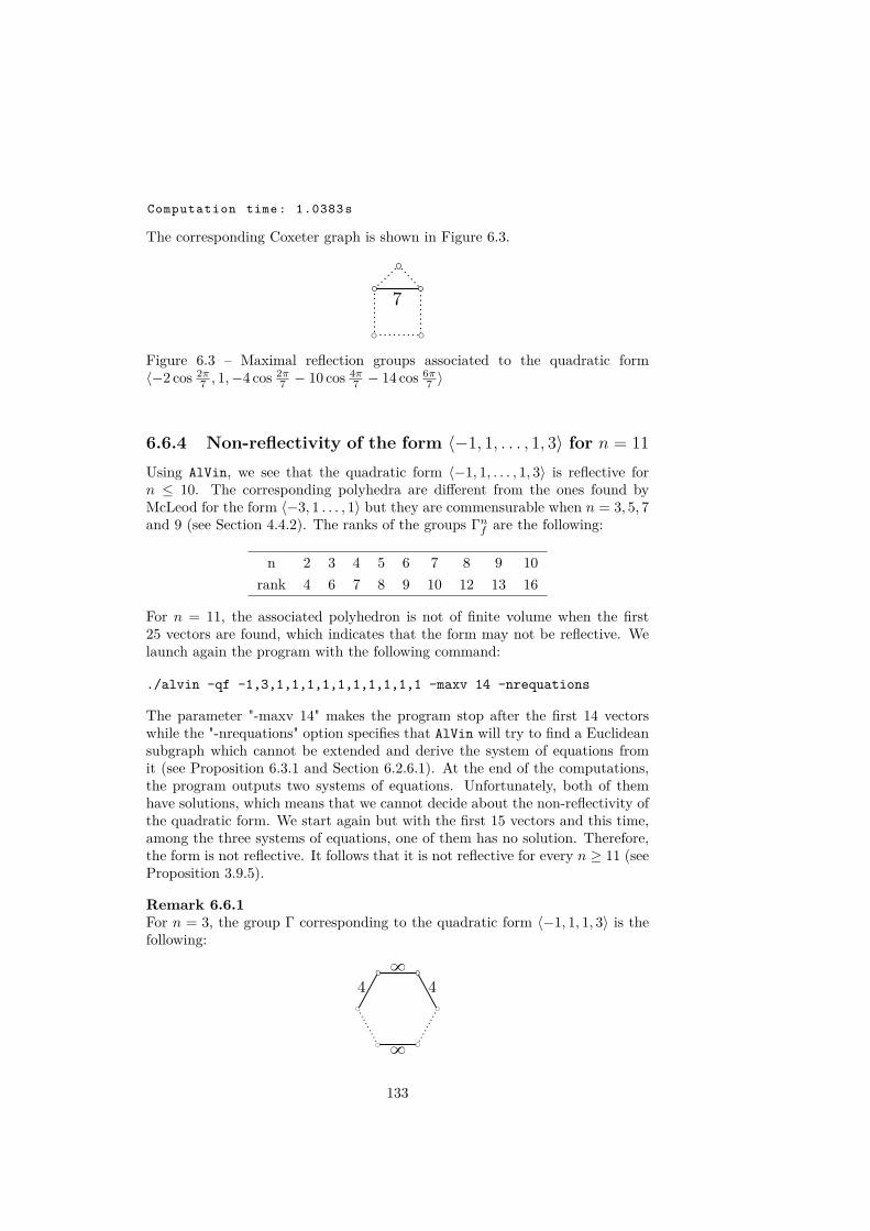
Computation time: 1.0383 s
The corresponding Coxeter graph is shown in Figure 6.3.
Figure 6.3 – Maximal reflection groups associated to the quadratic form〈−2 cos 2π
7 , 1,−4 cos 2π7 − 10 cos 4π
7 − 14 cos 6π7 〉
6.6.4 Non-reflectivity of the form 〈−1, 1, . . . , 1, 3〉 for n = 11Using AlVin, we see that the quadratic form 〈−1, 1, . . . , 1, 3〉 is reflective forn ≤ 10. The corresponding polyhedra are different from the ones found byMcLeod for the form 〈−3, 1 . . . , 1〉 but they are commensurable when n = 3, 5, 7and 9 (see Section 4.4.2). The ranks of the groups Γnf are the following:
n 2 3 4 5 6 7 8 9 10rank 4 6 7 8 9 10 12 13 16
For n = 11, the associated polyhedron is not of finite volume when the first25 vectors are found, which indicates that the form may not be reflective. Welaunch again the program with the following command:
./alvin -qf -1,3,1,1,1,1,1,1,1,1,1,1 -maxv 14 -nrequations
The parameter "-maxv 14" makes the program stop after the first 14 vectorswhile the "-nrequations" option specifies that AlVin will try to find a Euclideansubgraph which cannot be extended and derive the system of equations fromit (see Proposition 6.3.1 and Section 6.2.6.1). At the end of the computations,the program outputs two systems of equations. Unfortunately, both of themhave solutions, which means that we cannot decide about the non-reflectivity ofthe quadratic form. We start again but with the first 15 vectors and this time,among the three systems of equations, one of them has no solution. Therefore,the form is not reflective. It follows that it is not reflective for every n ≥ 11 (seeProposition 3.9.5).
Remark 6.6.1For n = 3, the group Γ corresponding to the quadratic form 〈−1, 1, 1, 3〉 is thefollowing:
133

Using [Kel91, Theorem 14.6], we can compute
covol Γ = L(π
6
)+ 1
2 L( π
12
)+ 1
2 L(
7π12
)' 0.634338504006034,
where L is the Lobachevsky function, defined by
L(x) = −∫ x
0log |2 sin t|dt, x ∈ R.
According to Scharlau’s classification, our group Γ is a subgroup of one of thefollowing groups in his list: Γ1, Γ6, Γ27, Γ38, Γ44, Γ47, Γ48 (see [Sch89, p. 21]).The group Γ1, corresponds to the group of units of the form 〈−3, 1, 1, 1〉 asshown by McLeod. It preserves a lattice of the same discriminant as the latticepreserved by Γ, which suggest that Γ ≤ Γ1. Moreover, using [RT13], we see that
covol Γ1 = 5√
364 · L(2,−3) ' 0.105723084010027,
where L(s,D) is the Dirichlet L-series given by
L(s, d) =∞∑k=1
(D
k
)k−s, s > 1,
where(Dk
)is a Kronecker symbol. Numerical computations show that the
quotient covol Γ/ covol Γ1 is equal to 6, up to machine precision. This stronglyindicates that Γ is a subgroup of index 6 in Γ1.
6.6.5 Non-reflectivity of the form 〈−1, 1, 1, 13〉The quadratic form 〈−1, 1, 13〉 is reflective and the rank of the associated reflec-tion group is 8. When running the algorithm with 〈−1, 1, 1, 13〉 we see that thecomponents of the vectors grow quickly and that more of 20 vectors are com-puted without the polyhedron
⋂iH−ei becoming of finite volume. The method
used for the example of Section 6.6.4 does not seem to work here: for a fewnumbers of vectors, we see that among the Euclidean subgraphs, there is nonewhich cannot we extended to a Euclidean graph of rank 2. We will thus seethat the form is not reflective by showing that the fundamental polyhedron Phas an infinite number of symmetries.
We again call the program as follows:./ alvin -qf -1,1,1,13 -maxv 15 -nr [5 ,6]
The option "-maxv 15" is to limit the search to the first 15 vectors. The lastoption indicates that AlVin will try to find integral symmetries of the funda-mental polyhedron by looking at involutions of subgraphs of sizes 5 and 6 (seeSection 6.2.6.2). The output is then the following:Quadratic form (3 ,1): -1, 1, 1, 13Field of definition : Q
Vectors :e1 = (0, -1, 1, 0)
134

e2 = (0, 0, -1, 0)e3 = (0, 0, 0, -1)e4 = (1, 1, 1, 0)e5 = (4, 2, 1, 1)e6 = (13, 13, 0, 1)e7 = (6, 5, 0, 1)e8 = (11, 2, 1, 3)e9 = (18, 1, 0, 5)e10 = (52, 13, 0, 14)e11 = (91, 13, 0, 25)e12 = (34, 25, 8, 6)e13 = (143 , 104, 39, 25)e14 = (72, 55, 17, 12)e15 = (312 , 234, 78, 53)
The algorithm did not terminate ; the polyhedron may be ofinfinite volume
Checking if the form is non - reflective ...The form is non - reflective
If we add the parameter "-debug" to get more information, we get at the endthe following additional data:Checking if the form is non - reflective ...
The form is non - reflectiveList of used involutions :
e2 <-> e4 , e3 <-> e6 , e5e1 <-> e5 , e2 , e3 <-> e10
It means that the two given permutations of vectors extend to two integralsymmetries of the polyhedron which don’t have common fixed points inside H3.Hence, the form is non-reflective.
Remark 6.6.2When trying to exploit this method to show that a quadratic form is not reflec-tive, there are two parameters:
1. the bounds for the size of the subgraphs;
2. the number "-maxv" of vectors to compute.
It is advised to start with small parameters to avoid long computations andthen gradually increase them. Usually, the bounds for the size of the subgraphscan be taken to be [n+ 1, n+ 2], [n+ 1, n+ 3] or [n+ 1, n+ 4]. If AlVin cannotconclude (this often happens when the roots can have many possible norms) butthe quadratic form is thought to be non-reflective, one can increase the numberof "maxv" vectors by small steps.
6.6.6 Running time for some well-known examplesThe following table gives some typical running time of AlVin. In some cases, alarge part of the computation time is allocated to check that the final polyhedronof the sequence has indeed finite volume.
135

n K form time (s)
18 Q 〈−1, 1, . . . , 1〉 170
14 Q 〈−2, 1, . . . , 1〉 0.3
13 Q 〈−3, 1, . . . , 1〉 0.2
6 Q[√
2] 〈−1−Θ2, 1, . . . , 1〉 16.8
7 Q[√
5] −Θ5, 1, . . . , 1 0.1
4 Q[cos 2π
7]〈−2 cos 2π
7 , 1, 1, 1, 1〉 9.5
6.7 Program testingConsider the quadratic form fnα = 〈−α, 1, . . . , 1〉 of signature (n, 1). We testedour program for the following quadratic form:
α n Reference1 2→ 19 [Vin72],[KV78]
2 2→ 14 [Vin72]
3 2→ 13 [Mcl11]
5 2→ 8 [Mar12]1+√
52 2→ 7 [Bug84]
1 +√
2 2→ 6 [Bug90]
2 cos 2π7 2→ 4 [Bug92]
The two-dimensional forms without square factors of [Gro08] were also com-pared. This corresponds to the following quadratic forms:
• 〈−1, 1, α〉 for α ∈ 1, 2, 3, 5, 6, 7, 10, 11, 13, 14;
• 〈−1, α, α〉 for α ∈ 1, 2, 3, 5, 6, 7, 10, 11.
6.8 Applications of the algorithmIn this section, we present numerous applications of the Vinberg algorithm,including new polyhedra and a classification of diagonal quadratic forms ofsignature (3, 1) with small coefficients. The applications are distributed in threeparts, according to the defining field of their quadratic form.
136
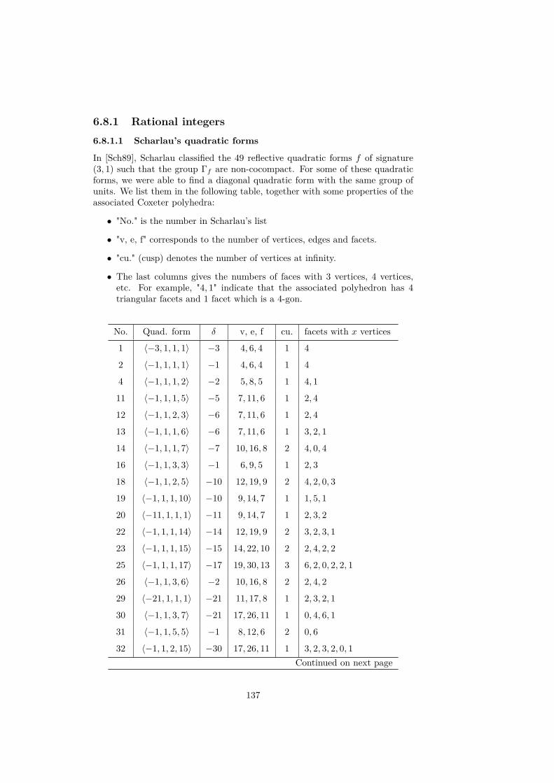
6.8.1 Rational integers6.8.1.1 Scharlau’s quadratic forms
In [Sch89], Scharlau classified the 49 reflective quadratic forms f of signature(3, 1) such that the group Γf are non-cocompact. For some of these quadraticforms, we were able to find a diagonal quadratic form with the same group ofunits. We list them in the following table, together with some properties of theassociated Coxeter polyhedra:
• "No." is the number in Scharlau’s list
• "v, e, f" corresponds to the number of vertices, edges and facets.
• "cu." (cusp) denotes the number of vertices at infinity.
• The last columns gives the numbers of faces with 3 vertices, 4 vertices,etc. For example, "4, 1" indicate that the associated polyhedron has 4triangular facets and 1 facet which is a 4-gon.
No. Quad. form δ v, e, f cu. facets with x vertices
1 〈−3, 1, 1, 1〉 −3 4, 6, 4 1 4
2 〈−1, 1, 1, 1〉 −1 4, 6, 4 1 4
4 〈−1, 1, 1, 2〉 −2 5, 8, 5 1 4, 1
11 〈−1, 1, 1, 5〉 −5 7, 11, 6 1 2, 4
12 〈−1, 1, 2, 3〉 −6 7, 11, 6 1 2, 4
13 〈−1, 1, 1, 6〉 −6 7, 11, 6 1 3, 2, 1
14 〈−1, 1, 1, 7〉 −7 10, 16, 8 2 4, 0, 4
16 〈−1, 1, 3, 3〉 −1 6, 9, 5 1 2, 3
18 〈−1, 1, 2, 5〉 −10 12, 19, 9 2 4, 2, 0, 3
19 〈−1, 1, 1, 10〉 −10 9, 14, 7 1 1, 5, 1
20 〈−11, 1, 1, 1〉 −11 9, 14, 7 1 2, 3, 2
22 〈−1, 1, 1, 14〉 −14 12, 19, 9 2 3, 2, 3, 1
23 〈−1, 1, 1, 15〉 −15 14, 22, 10 2 2, 4, 2, 2
25 〈−1, 1, 1, 17〉 −17 19, 30, 13 3 6, 2, 0, 2, 2, 1
26 〈−1, 1, 3, 6〉 −2 10, 16, 8 2 2, 4, 2
29 〈−21, 1, 1, 1〉 −21 11, 17, 8 1 2, 3, 2, 1
30 〈−1, 1, 3, 7〉 −21 17, 26, 11 1 0, 4, 6, 1
31 〈−1, 1, 5, 5〉 −1 8, 12, 6 2 0, 6
32 〈−1, 1, 2, 15〉 −30 17, 26, 11 1 3, 2, 3, 2, 0, 1Continued on next page
137

No. Quad. form δ v, e, f cu. facets with x vertices
33 〈−1, 1, 1, 30〉 −30 22, 34, 14 2 2, 4, 2, 6
34 〈−1, 1, 5, 6〉 −30 20, 31, 13 2 2, 6, 2, 0, 2, 1
35 〈−1, 1, 3, 10〉 −30 22, 34, 14 2 0, 8, 2, 2, 2
37 〈−35, 1, 1, 1〉 −35 17, 26, 11 1 0, 4, 6, 1
39 〈−1, 1, 6, 7〉 −42 30, 46, 18 2 4, 2, 6, 0, 6
40 〈−1, 1, 3, 14〉 −42 30, 46, 18 2 0, 6, 8, 1, 2, 1
41 〈−1, 1, 3, 15〉 −5 23, 36, 15 3 2, 6, 0, 7
42 〈−1, 1, 7, 7〉 −1 14, 21, 9 2 0, 3, 6
43 〈−1, 1, 5, 10〉 −2 20, 31, 13 2 0, 8, 0, 5
45 〈−1, 1, 6, 15〉 −10 34, 52, 20 2 4, 2, 6, 6, 0, 0, 2
46 〈−1, 1, 3, 30〉 −10 34, 52, 20 2 0, 10, 4, 3, 2, 0, 0, 0, 0, 1
49 〈−1, 1, 15, 15〉 −1 32, 48, 18 4 0, 4, 4, 10
6.8.1.2 Classification of diagonal quadratic forms of signature (3, 1)with small coefficients
We consider diagonal quadratic forms 〈−α0, α1, α2, α3〉 where αi ∈ 1, 2, 3, 5,6, 7, 10. Up to the ordering of the coefficients α1, α2 and α3, there are 543of them. For each such quadratic form, we test whether it is reflective or notand we classify the associated maximal subgroup generated by reflections up tocommensurability and isomorphism.
Among the 543 forms, 248 of them are non-reflective and 295 are reflective.The latter ones give rise to groups which fall into 20 commensurability classesand 49 isomorphism classes. In the tables below, we omit the form brackets 〈 〉for brevity.
Non-reflective forms The 248 non-reflective are the following:
−10, 1, 1, 7 −10, 1, 2, 5 −10, 1, 2, 7 −10, 1, 3, 6 −10, 1, 3, 7−10, 1, 5, 7 −10, 1, 6, 7 −10, 1, 6, 10 −10, 1, 7, 7 −10, 1, 7, 10−10, 2, 2, 7 −10, 2, 3, 7 −10, 2, 3, 10 −10, 2, 5, 7 −10, 2, 6, 7−10, 2, 7, 7 −10, 2, 7, 10 −10, 3, 3, 7 −10, 3, 3, 10 −10, 3, 5, 6−10, 3, 5, 7 −10, 3, 6, 7 −10, 3, 6, 10 −10, 3, 7, 7 −10, 3, 7, 10−10, 5, 5, 7 −10, 5, 6, 7 −10, 5, 7, 7 −10, 5, 7, 10 −10, 6, 6, 7−10, 6, 7, 7 −10, 6, 7, 10 −10, 7, 7, 7 −10, 7, 7, 10 −10, 7, 10, 10−7, 1, 1, 2 −7, 1, 1, 3 −7, 1, 1, 5 −7, 1, 1, 6 −7, 1, 1, 10
Continued on next page
138
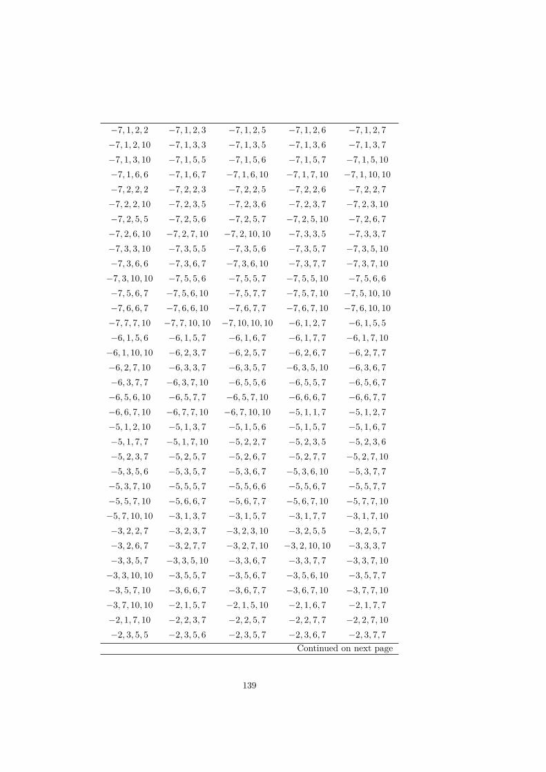
−7, 1, 2, 2 −7, 1, 2, 3 −7, 1, 2, 5 −7, 1, 2, 6 −7, 1, 2, 7−7, 1, 2, 10 −7, 1, 3, 3 −7, 1, 3, 5 −7, 1, 3, 6 −7, 1, 3, 7−7, 1, 3, 10 −7, 1, 5, 5 −7, 1, 5, 6 −7, 1, 5, 7 −7, 1, 5, 10−7, 1, 6, 6 −7, 1, 6, 7 −7, 1, 6, 10 −7, 1, 7, 10 −7, 1, 10, 10−7, 2, 2, 2 −7, 2, 2, 3 −7, 2, 2, 5 −7, 2, 2, 6 −7, 2, 2, 7−7, 2, 2, 10 −7, 2, 3, 5 −7, 2, 3, 6 −7, 2, 3, 7 −7, 2, 3, 10−7, 2, 5, 5 −7, 2, 5, 6 −7, 2, 5, 7 −7, 2, 5, 10 −7, 2, 6, 7−7, 2, 6, 10 −7, 2, 7, 10 −7, 2, 10, 10 −7, 3, 3, 5 −7, 3, 3, 7−7, 3, 3, 10 −7, 3, 5, 5 −7, 3, 5, 6 −7, 3, 5, 7 −7, 3, 5, 10−7, 3, 6, 6 −7, 3, 6, 7 −7, 3, 6, 10 −7, 3, 7, 7 −7, 3, 7, 10−7, 3, 10, 10 −7, 5, 5, 6 −7, 5, 5, 7 −7, 5, 5, 10 −7, 5, 6, 6−7, 5, 6, 7 −7, 5, 6, 10 −7, 5, 7, 7 −7, 5, 7, 10 −7, 5, 10, 10−7, 6, 6, 7 −7, 6, 6, 10 −7, 6, 7, 7 −7, 6, 7, 10 −7, 6, 10, 10−7, 7, 7, 10 −7, 7, 10, 10 −7, 10, 10, 10 −6, 1, 2, 7 −6, 1, 5, 5−6, 1, 5, 6 −6, 1, 5, 7 −6, 1, 6, 7 −6, 1, 7, 7 −6, 1, 7, 10−6, 1, 10, 10 −6, 2, 3, 7 −6, 2, 5, 7 −6, 2, 6, 7 −6, 2, 7, 7−6, 2, 7, 10 −6, 3, 3, 7 −6, 3, 5, 7 −6, 3, 5, 10 −6, 3, 6, 7−6, 3, 7, 7 −6, 3, 7, 10 −6, 5, 5, 6 −6, 5, 5, 7 −6, 5, 6, 7−6, 5, 6, 10 −6, 5, 7, 7 −6, 5, 7, 10 −6, 6, 6, 7 −6, 6, 7, 7−6, 6, 7, 10 −6, 7, 7, 10 −6, 7, 10, 10 −5, 1, 1, 7 −5, 1, 2, 7−5, 1, 2, 10 −5, 1, 3, 7 −5, 1, 5, 6 −5, 1, 5, 7 −5, 1, 6, 7−5, 1, 7, 7 −5, 1, 7, 10 −5, 2, 2, 7 −5, 2, 3, 5 −5, 2, 3, 6−5, 2, 3, 7 −5, 2, 5, 7 −5, 2, 6, 7 −5, 2, 7, 7 −5, 2, 7, 10−5, 3, 5, 6 −5, 3, 5, 7 −5, 3, 6, 7 −5, 3, 6, 10 −5, 3, 7, 7−5, 3, 7, 10 −5, 5, 5, 7 −5, 5, 6, 6 −5, 5, 6, 7 −5, 5, 7, 7−5, 5, 7, 10 −5, 6, 6, 7 −5, 6, 7, 7 −5, 6, 7, 10 −5, 7, 7, 10−5, 7, 10, 10 −3, 1, 3, 7 −3, 1, 5, 7 −3, 1, 7, 7 −3, 1, 7, 10−3, 2, 2, 7 −3, 2, 3, 7 −3, 2, 3, 10 −3, 2, 5, 5 −3, 2, 5, 7−3, 2, 6, 7 −3, 2, 7, 7 −3, 2, 7, 10 −3, 2, 10, 10 −3, 3, 3, 7−3, 3, 5, 7 −3, 3, 5, 10 −3, 3, 6, 7 −3, 3, 7, 7 −3, 3, 7, 10−3, 3, 10, 10 −3, 5, 5, 7 −3, 5, 6, 7 −3, 5, 6, 10 −3, 5, 7, 7−3, 5, 7, 10 −3, 6, 6, 7 −3, 6, 7, 7 −3, 6, 7, 10 −3, 7, 7, 10−3, 7, 10, 10 −2, 1, 5, 7 −2, 1, 5, 10 −2, 1, 6, 7 −2, 1, 7, 7−2, 1, 7, 10 −2, 2, 3, 7 −2, 2, 5, 7 −2, 2, 7, 7 −2, 2, 7, 10−2, 3, 5, 5 −2, 3, 5, 6 −2, 3, 5, 7 −2, 3, 6, 7 −2, 3, 7, 7
Continued on next page
139

−2, 3, 7, 10 −2, 3, 10, 10 −2, 5, 5, 7 −2, 5, 6, 7 −2, 5, 7, 7−2, 5, 7, 10 −2, 6, 7, 7 −2, 6, 7, 10 −2, 7, 7, 7 −2, 7, 7, 10−2, 7, 10, 10 −1, 1, 5, 7 −1, 1, 7, 10 −1, 2, 5, 7 −1, 2, 5, 10−1, 2, 6, 7 −1, 2, 7, 7 −1, 2, 7, 10 −1, 3, 5, 7 −1, 3, 6, 7−1, 3, 6, 10 −1, 3, 7, 10 −1, 5, 5, 6 −1, 5, 5, 7 −1, 5, 6, 7−1, 5, 7, 7 −1, 5, 7, 10 −1, 6, 6, 7 −1, 6, 7, 7 −1, 6, 7, 10−1, 6, 10, 10 −1, 7, 7, 10 −1, 7, 10, 10
Reflective forms The reflective forms are presented by their commensurabil-ity invariants and isomorphism classes. The rank of the groups ranges between4 and 22. The following table presents the number of groups with a given rank.
4 5 6 7 8 9 10 11 13 14 15 18 19 20 225 8 58 12 15 30 19 14 22 48 1 19 8 20 16
The classification of the reflective forms is presented in the following tables.
Q,−1, −1, 1, 1, 1−2, 1, 1, 2 −1, 1, 2, 2−3, 1, 1, 3 −1, 1, 3, 3−5, 1, 1, 5 −1, 1, 5, 5−7, 1, 1, 7 −1, 1, 7, 7−5, 3, 3, 5 −3, 3, 5, 5−10, 1, 1, 10 −5, 2, 2, 5 −2, 2, 5, 5 −1, 1, 10, 10−6, 1, 1, 6 −6, 1, 2, 3 −3, 1, 2, 6 −3, 2, 2, 3−2, 1, 3, 6 −2, 2, 3, 3 −1, 1, 6, 6 −1, 2, 3, 6
Q,−10, −10, 1, 1, 1 −10, 1, 10, 10 −5, 2, 2, 2 −5, 2, 5, 5−2, 2, 2, 5 −2, 5, 5, 5 −1, 1, 1, 10 −1, 10, 10, 10−10, 1, 3, 3 −10, 2, 3, 6 −6, 1, 6, 10 −5, 1, 3, 6−5, 2, 6, 6 −3, 2, 3, 5 −2, 3, 6, 10 −2, 5, 6, 6−1, 3, 3, 10 −1, 3, 5, 6−10, 1, 6, 6 −6, 1, 3, 5 −6, 2, 3, 10 −6, 2, 5, 6−5, 2, 3, 3 −3, 1, 3, 10 −3, 1, 5, 6 −3, 2, 6, 10−2, 3, 3, 5 −1, 6, 6, 10−10, 1, 2, 2 −10, 1, 5, 5 −10, 2, 5, 10 −5, 1, 1, 2−5, 1, 5, 10 −5, 2, 10, 10 −2, 1, 1, 5 −2, 1, 2, 10
Continued on next page
140

−2, 5, 10, 10 −1, 1, 2, 5 −1, 2, 2, 10 −1, 5, 5, 10
Q,−14, 3 −7, 2, 3, 3 −7, 2, 6, 6 −6, 1, 3, 7 −3, 1, 6, 7−2, 3, 3, 7 −2, 6, 6, 7
Q,−14, −7, 2, 7, 7 −2, 1, 1, 7 −2, 2, 2, 7 −1, 1, 2, 7
Q,−15, 2 −3, 1, 1, 5−5, 3, 3, 3 −3, 5, 5, 5−10, 1, 2, 3 −10, 3, 3, 6 −6, 1, 1, 10 −6, 5, 5, 10−5, 1, 2, 6 −5, 3, 6, 6 −3, 2, 2, 5 −3, 5, 10, 10−2, 1, 3, 10 −2, 1, 5, 6 −1, 2, 3, 10 −1, 2, 5, 6
Q,−15, −10, 1, 1, 6 −10, 3, 5, 10 −10, 5, 5, 6 −6, 1, 2, 5−6, 3, 3, 10 −6, 3, 5, 6 −5, 1, 1, 3 −5, 2, 2, 3−5, 3, 5, 5 −5, 3, 10, 10 −5, 5, 6, 10 −3, 1, 2, 10−3, 3, 3, 5 −3, 3, 6, 10 −3, 5, 6, 6 −2, 2, 3, 5−1, 1, 3, 5 −1, 1, 6, 10
Q,−2, 3 −6, 1, 1, 3 −6, 2, 2, 3 −3, 1, 1, 6 −3, 2, 2, 6−2, 1, 3, 3 −2, 1, 6, 6 −1, 2, 3, 3 −1, 2, 6, 6−10, 3, 3, 5 −10, 5, 6, 6 −6, 3, 5, 5 −6, 3, 10, 10−5, 3, 3, 10 −5, 6, 6, 10 −3, 5, 5, 6 −3, 6, 10, 10
Q,−2, −2, 1, 1, 1 −2, 1, 2, 2 −1, 1, 1, 2 −1, 2, 2, 2−6, 1, 2, 6 −3, 1, 2, 3 −2, 2, 3, 6 −1, 1, 3, 6−10, 1, 1, 5 −10, 1, 2, 10 −10, 2, 2, 5 −5, 1, 1, 10−5, 1, 2, 5 −5, 2, 2, 10 −2, 1, 5, 5 −2, 1, 10, 10−2, 2, 5, 10 −1, 1, 5, 10 −1, 2, 5, 5 −1, 2, 10, 10
Q,−21, −1, 1, 3, 7−7, 3, 3, 3 −3, 1, 1, 7 −3, 7, 7, 7
Q,−3, 7 −1, 3, 7, 7
Q,−3, −3, 1, 5, 5−3, 1, 1, 1 −1, 3, 3, 3−6, 1, 1, 2 −6, 1, 3, 6 −6, 2, 3, 3 −3, 1, 2, 2−3, 1, 3, 3 −3, 1, 6, 6 −3, 2, 3, 6 −2, 1, 1, 6−2, 1, 2, 3 −2, 3, 3, 6 −1, 1, 1, 3 −1, 1, 2, 6−1, 2, 2, 3 −1, 3, 6, 6−10, 1, 3, 10 −10, 1, 5, 6 −10, 2, 3, 5 −6, 1, 5, 10−6, 2, 5, 5 −5, 1, 3, 5 −5, 1, 6, 10 −5, 2, 3, 10−5, 2, 5, 6 −3, 1, 10, 10 −3, 2, 5, 10 −2, 3, 5, 10
Continued on next page
141
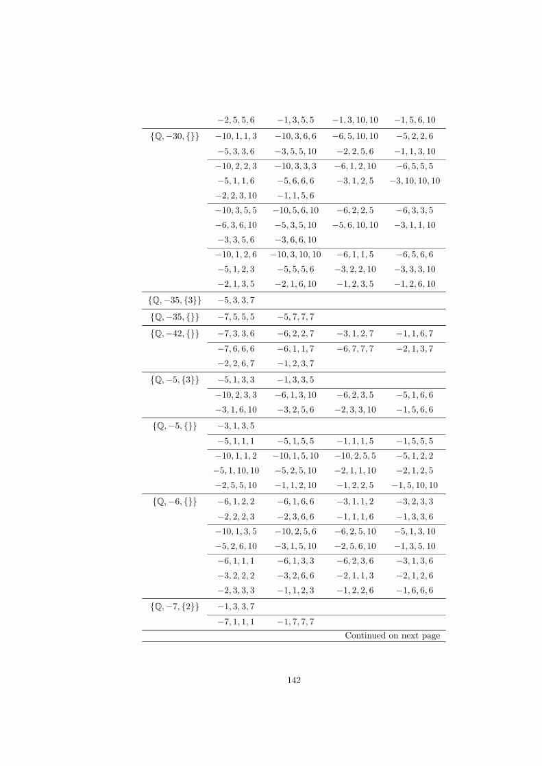
−2, 5, 5, 6 −1, 3, 5, 5 −1, 3, 10, 10 −1, 5, 6, 10
Q,−30, −10, 1, 1, 3 −10, 3, 6, 6 −6, 5, 10, 10 −5, 2, 2, 6−5, 3, 3, 6 −3, 5, 5, 10 −2, 2, 5, 6 −1, 1, 3, 10−10, 2, 2, 3 −10, 3, 3, 3 −6, 1, 2, 10 −6, 5, 5, 5−5, 1, 1, 6 −5, 6, 6, 6 −3, 1, 2, 5 −3, 10, 10, 10−2, 2, 3, 10 −1, 1, 5, 6−10, 3, 5, 5 −10, 5, 6, 10 −6, 2, 2, 5 −6, 3, 3, 5−6, 3, 6, 10 −5, 3, 5, 10 −5, 6, 10, 10 −3, 1, 1, 10−3, 3, 5, 6 −3, 6, 6, 10−10, 1, 2, 6 −10, 3, 10, 10 −6, 1, 1, 5 −6, 5, 6, 6−5, 1, 2, 3 −5, 5, 5, 6 −3, 2, 2, 10 −3, 3, 3, 10−2, 1, 3, 5 −2, 1, 6, 10 −1, 2, 3, 5 −1, 2, 6, 10
Q,−35, 3 −5, 3, 3, 7
Q,−35, −7, 5, 5, 5 −5, 7, 7, 7
Q,−42, −7, 3, 3, 6 −6, 2, 2, 7 −3, 1, 2, 7 −1, 1, 6, 7−7, 6, 6, 6 −6, 1, 1, 7 −6, 7, 7, 7 −2, 1, 3, 7−2, 2, 6, 7 −1, 2, 3, 7
Q,−5, 3 −5, 1, 3, 3 −1, 3, 3, 5−10, 2, 3, 3 −6, 1, 3, 10 −6, 2, 3, 5 −5, 1, 6, 6−3, 1, 6, 10 −3, 2, 5, 6 −2, 3, 3, 10 −1, 5, 6, 6
Q,−5, −3, 1, 3, 5−5, 1, 1, 1 −5, 1, 5, 5 −1, 1, 1, 5 −1, 5, 5, 5−10, 1, 1, 2 −10, 1, 5, 10 −10, 2, 5, 5 −5, 1, 2, 2−5, 1, 10, 10 −5, 2, 5, 10 −2, 1, 1, 10 −2, 1, 2, 5−2, 5, 5, 10 −1, 1, 2, 10 −1, 2, 2, 5 −1, 5, 10, 10
Q,−6, −6, 1, 2, 2 −6, 1, 6, 6 −3, 1, 1, 2 −3, 2, 3, 3−2, 2, 2, 3 −2, 3, 6, 6 −1, 1, 1, 6 −1, 3, 3, 6−10, 1, 3, 5 −10, 2, 5, 6 −6, 2, 5, 10 −5, 1, 3, 10−5, 2, 6, 10 −3, 1, 5, 10 −2, 5, 6, 10 −1, 3, 5, 10−6, 1, 1, 1 −6, 1, 3, 3 −6, 2, 3, 6 −3, 1, 3, 6−3, 2, 2, 2 −3, 2, 6, 6 −2, 1, 1, 3 −2, 1, 2, 6−2, 3, 3, 3 −1, 1, 2, 3 −1, 2, 2, 6 −1, 6, 6, 6
Q,−7, 2 −1, 3, 3, 7−7, 1, 1, 1 −1, 7, 7, 7
Continued on next page
142
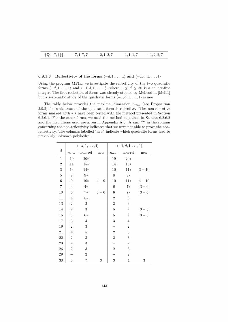
Q,−7, −7, 1, 7, 7 −2, 1, 2, 7 −1, 1, 1, 7 −1, 2, 2, 7
6.8.1.3 Reflectivity of the forms 〈−d, 1, . . . , 1〉 and 〈−1, d, 1, . . . , 1〉
Using the program AlVin, we investigate the reflectivity of the two quadraticforms 〈−d, 1, . . . , 1〉 and 〈−1, d, 1, . . . , 1〉, where 1 ≤ d ≤ 30 is a square-freeinteger. The first collection of forms was already studied by McLeod in [Mcl11]but a systematic study of the quadratic forms 〈−1, d, 1, . . . , 1〉 is new.
The table below provides the maximal dimension nmax (see Proposition3.9.5) for which each of the quadratic form is reflective. The non-reflectiveforms marked with a ∗ have been tested with the method presented in Section6.2.6.1. For the other forms, we used the method explained in Section 6.2.6.2and the involutions used are given in Appendix A.3. A sign "?" in the columnconcerning the non-reflectivity indicates that we were not able to prove the non-reflectivity. The columns labelled "new" indicate which quadratic forms lead topreviously unknown polyhedra.
d〈−d, 1, . . . , 1〉 〈−1, d, 1, . . . , 1〉
nmax non-ref new nmax non-ref new1 19 20∗ 19 20∗2 14 15∗ 14 15∗3 13 14∗ 10 11∗ 3− 105 8 9∗ 8 9∗6 9 10∗ 4− 9 10 11∗ 4− 107 3 4∗ 6 7∗ 3− 610 6 7∗ 3− 6 6 7∗ 3− 611 4 5∗ 2 313 2 3 2 314 2 3 5 ? 3− 515 5 6∗ 5 ? 3− 517 3 4 3 419 2 3 − 221 4 5 2 322 2 3 2 323 2 3 − 226 2 3 2 329 − 2 − 230 3 ? 3 3 4 3
143
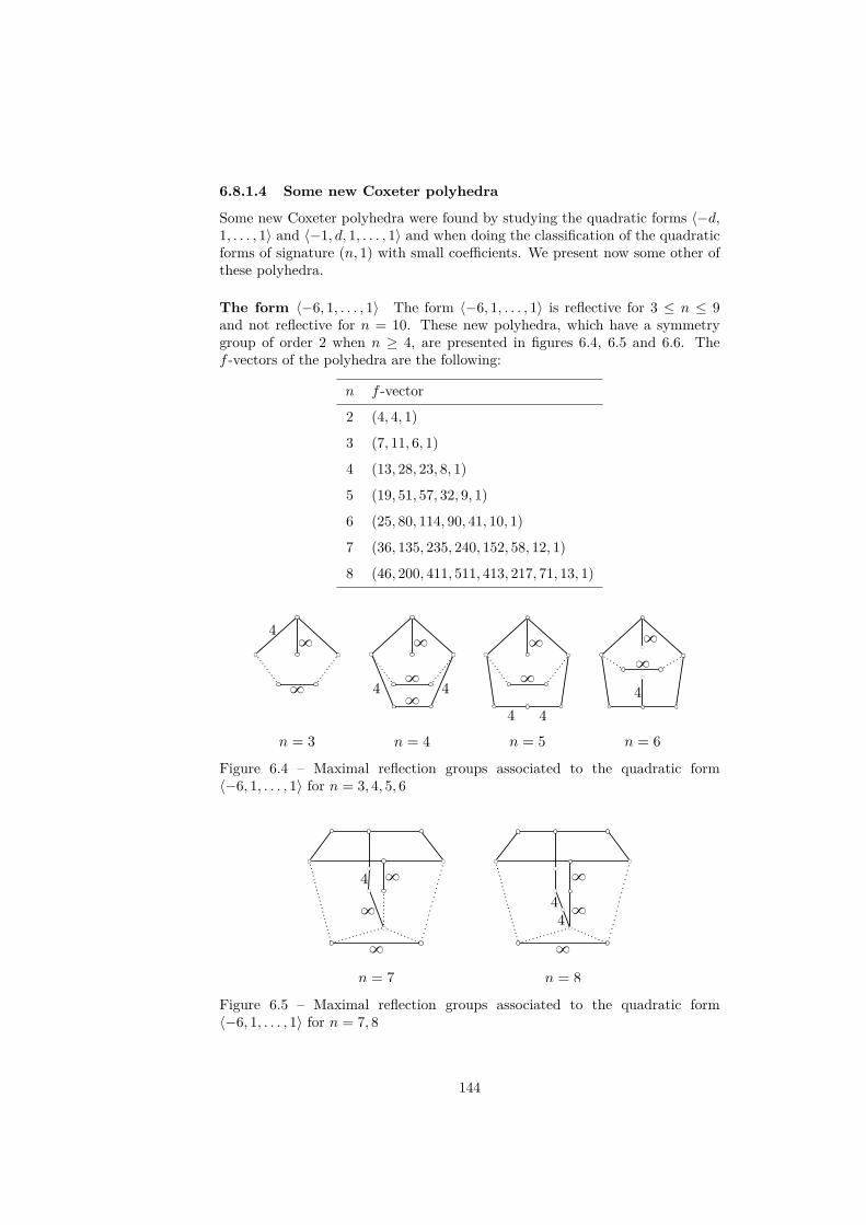
6.8.1.4 Some new Coxeter polyhedra
Some new Coxeter polyhedra were found by studying the quadratic forms 〈−d,1, . . . , 1〉 and 〈−1, d, 1, . . . , 1〉 and when doing the classification of the quadraticforms of signature (n, 1) with small coefficients. We present now some other ofthese polyhedra.
The form 〈−6, 1, . . . , 1〉 The form 〈−6, 1, . . . , 1〉 is reflective for 3 ≤ n ≤ 9and not reflective for n = 10. These new polyhedra, which have a symmetrygroup of order 2 when n ≥ 4, are presented in figures 6.4, 6.5 and 6.6. Thef -vectors of the polyhedra are the following:
n f -vector
2 (4, 4, 1)
3 (7, 11, 6, 1)
4 (13, 28, 23, 8, 1)
5 (19, 51, 57, 32, 9, 1)
6 (25, 80, 114, 90, 41, 10, 1)
7 (36, 135, 235, 240, 152, 58, 12, 1)
8 (46, 200, 411, 511, 413, 217, 71, 13, 1)
Figure 6.4 – Maximal reflection groups associated to the quadratic form〈−6, 1, . . . , 1〉 for n = 3, 4, 5, 6
Figure 6.5 – Maximal reflection groups associated to the quadratic form〈−6, 1, . . . , 1〉 for n = 7, 8
144

Figure 6.6 – Maximal reflection group associated to the quadratic form 〈−6, 1,1, . . . , 1〉 of signature (9, 1)
6.8.1.5 Cocompact groups with k = Q
The following quadratic forms are reflective and anisotropic, which implies thatthe associated polyhedra are compact (see Remark 3.9.2). For each form, wegive the p-adic field Qp over which the form is anisotropic, together with thef -vector of the associated Coxeter polyhedron in H3.
Quad. form anis. over f − vector
〈−1, 2, 3, 3〉 Q3 (8, 12, 6, 1)
〈−1, 2, 6, 6〉 Q3 (8, 12, 6, 1)
〈−7, 1, 1, 1〉 Q2 (6, 9, 5, 1)
〈−1, 3, 3, 5〉 Q3 (10, 15, 7, 1)
〈−15, 1, 1, 1〉 Q2 (8, 12, 6, 1)
〈−6, 2, 2, 3〉 Q3 (8, 12, 6, 1)
6.8.1.6 About the combinatorics
For a reflective quadratic form, it seems impossible to predict the f -vector f(P )of the associated Coxeter polyhedron P ⊂ Hn, or even the rank of the groupΓf , which can be big when compared with the dimension n, as shown in Table6.7.
6.8.1.7 Errors in literature
As mentioned above, Lemma 3.1.5 of [Mcl13] is true only if d is prime. Thisleads in particular to incorrect groups when d = 6, 15, 30, 33, 39. Moreover, theform 〈−d, 1, . . . , 1〉 is reflective at least until n = 6 when d = 6 and is reflectiveexactly when n ≤ 6 for d = 10 (compare to [Mcl13, Table 3.1]).
145

n Quad. form cusps invariant f(P )
3 〈−1, 2, 2, 3〉 1 Q,−3, (7, 11, 6, 1)
4 〈−1, 2, 2, 3, 3〉 2 Q, 3,∞ (18, 38, 29, 9, 1)
5 〈−1, 2, 2, 3, 3, 3〉 10 Q, 3, (66, 188, 193, 85, 16, 1)
6 〈−1, 2, 2, 3, 3, 3, 3〉 57 Q, 2,∞ (653, 2286, 2896, 1660, 444,47, 1)
7 〈−1, 2, 2, 3, 3, 3, 3, 3〉 328 Q,−3, (4536, 19136, 29816, 22364,8684, 1654, 120, 1)
Table 6.7 – The forms 〈−1, 2, 2, 3, . . . , 3〉
6.8.2 Maximal real subfield of the 7-cyclotomic fieldUnfortunately, it seems that our implementation of the algorithm for the fieldK = Q[cos 2π
7 ] does not lead to new polyhedra in dimensions above 3. Oneof the reason is that our method for solving the norm equation is not suitablewhen the degree of the number field increases.
We give here two quadratic forms of signature (2, 1) which are reflective(recall that the integers between the brackets give the decomposition of theelement in the standard Z-basis, as indicated in Section 6.5.3):
• 〈[−1, 0, 0], 1, [−2,−4,−4]〉
• 〈[−1, 0, 0], 1, [−2,−5,−7]〉
6.8.3 Quadratic integers
6.8.3.1 Some reflective forms
We present some reflective quadratic forms over the first quadratic fields. Itfollows from equation (6.2) page 112 that the number of possibilities for thenorm (e, e) of a root grows exponentially with the number of prime factorswhich divide one of the factor of the quadratic form. Therefore, we consideronly quadratic forms with a few prime factors. As above, we denote by fα thequadratic form 〈−α, 1, . . . , 1〉.
In what follows, we denote by Θd the generator of the ring of integers ofQ[√d], that is, Θd =
√d if d ≡ 2, 3 mod 4 and Θd = 1+
√d
2 if d ≡ 1 mod 4.
Over Q[√
2] The following quadratic forms are reflective:
• 〈−Θ2, 3 + Θ2, 1, 1〉
• 〈−Θ2, 2 + Θ2, 1, 1, 1, 1〉
• 〈1− 2Θ2, 1, 1, 1, 1〉
• 〈1− 2Θ2, 3 + Θ2, 1〉
146
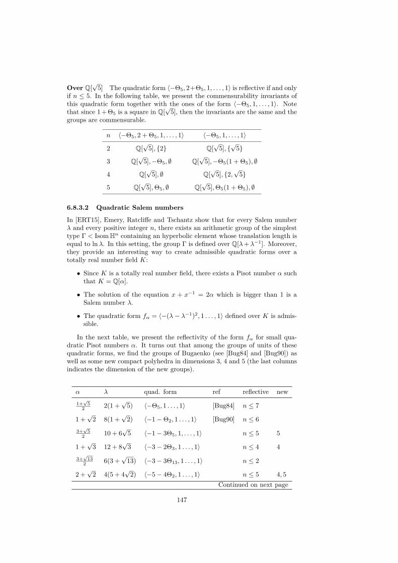
Over Q[√
5] The quadratic form 〈−Θ5, 2+Θ5, 1, . . . , 1〉 is reflective if and onlyif n ≤ 5. In the following table, we present the commensurability invariants ofthis quadratic form together with the ones of the form 〈−Θ5, 1, . . . , 1〉. Notethat since 1 + Θ5 is a square in Q[
√5], then the invariants are the same and the
groups are commensurable.
n 〈−Θ5, 2 + Θ5, 1, . . . , 1〉 〈−Θ5, 1, . . . , 1〉
2 Q[√
5], 2 Q[√
5], √
5
3 Q[√
5],−Θ5, ∅ Q[√
5],−Θ5(1 + Θ5), ∅
4 Q[√
5], ∅ Q[√
5], 2,√
5
5 Q[√
5],Θ5, ∅ Q[√
5],Θ5(1 + Θ5), ∅
6.8.3.2 Quadratic Salem numbers
In [ERT15], Emery, Ratcliffe and Tschantz show that for every Salem numberλ and every positive integer n, there exists an arithmetic group of the simplesttype Γ < IsomHn containing an hyperbolic element whose translation length isequal to lnλ. In this setting, the group Γ is defined over Q[λ+λ−1]. Moreover,they provide an interesting way to create admissible quadratic forms over atotally real number field K:
• Since K is a totally real number field, there exists a Pisot number α suchthat K = Q[α].
• The solution of the equation x + x−1 = 2α which is bigger than 1 is aSalem number λ.
• The quadratic form fα = 〈−(λ− λ−1)2, 1 . . . , 1〉 defined over K is admis-sible.
In the next table, we present the reflectivity of the form fα for small qua-dratic Pisot numbers α. It turns out that among the groups of units of thesequadratic forms, we find the groups of Bugaenko (see [Bug84] and [Bug90]) aswell as some new compact polyhedra in dimensions 3, 4 and 5 (the last columnsindicates the dimension of the new groups).
α λ quad. form ref reflective new1+√
52 2(1 +
√5) 〈−Θ5, 1 . . . , 1〉 [Bug84] n ≤ 7
1 +√
2 8(1 +√
2) 〈−1−Θ2, 1 . . . , 1〉 [Bug90] n ≤ 63+√
52 10 + 6
√5 〈−1− 3Θ5, 1, . . . , 1〉 n ≤ 5 5
1 +√
3 12 + 8√
3 〈−3− 2Θ3, 1 . . . , 1〉 n ≤ 4 43+√
132 6(3 +
√13) 〈−3− 3Θ13, 1 . . . , 1〉 n ≤ 2
2 +√
2 4(5 + 4√
2) 〈−5− 4Θ2, 1 . . . , 1〉 n ≤ 5 4, 5Continued on next page
147

α λ quad. form ref reflective new3+√
172 22 + 6
√17 〈2−Θ17, 1, . . . , 1〉 n ≤ 3 3
2 +√
3 8(3 + 2√
3) 〈−Θ3, 1, . . . , 1〉 n ≤ 3 33+√
212 26 + 6
√21 〈−5− 3Θ21, 1, . . . , 1〉 ?
2 +√
5 16(2 +√
5) 〈−1− 2Θ5, 1 . . . , 1〉 [Bug84] n ≤ 7
Remarks:
• When the considered quadratic forms are reflective, the associated groupΓ often has a small rank n + k, k ≥ 1, compared to the dimension n.However, this is not always the case. For example, for α = 2 +
√2 and
n = 5 we find a polyhedron whose f -vector is (96, 240, 228, 102, 20, 1), sothat the rank of Γ equals 20.
• The values α = 1 +√
3, 3+√
52 , 2 +
√2, 3+
√17
2 and 2 +√
3 lead to newpolyhedra. The value α = 2 +
√3 gives rise to Coxeter diagrams with
weight 12.
• For α = 3+√
212 and n = 2, we were not able to decide whether the qua-
dratic form is reflective or not.
6.8.3.3 Errors in literature
In [Mcl13], the vector e4 for the quadratic form 〈−1−4·Θ5, 1, 1〉 is (2+4·Θ5, 7+10 · Θ5, 1). However, the vector (1 + Θ5, 1 + 4 · Θ5, 0) seems to be admissibleand have a smaller fraction (1.5 compared to 35.9). It seems that non-integerpossible values for (e, e) were forgotten. The same issue seems to apply to theform 〈5−4 ·Θ5, 1, 1〉. This leads to incorrect polytopes (i.e. some of the normalvectors he found contain errors).
148
CHAPTER 7Index two subgroups and an infinite sequence
In [Gal05], Gal explains when a Coxeter group arises as a semi-direct product oftwo Coxeter subgroups, with one of them being a standard parabolic subgroup,and gives the presentation of the two subgroups. We will present his result andthen study the situation when one of the two subgroups is of index two. Wewill see that under certain conditions, this construction gives rise to an infinitesequence of index two subgroups. Our sequence of abstract Coxeter groupsgeneralizes the geometric approach described by Allcock : in [All06], he gave acondition under which a hyperbolic Coxeter polyhedron gives rise to an infinitesequence of polyhedra called "doublings".
In the first section, we will describe a way to construct an index two Coxetersubgroup Γ1 of a given abstract Coxeter group Γ and give the explicit presen-tation of the subgroup. In the second section, we will see that under a simpleassumption this process may be repeated to give rise to an infinite sequence ofindex two subgroups
Γ > Γ1 > Γ2 > . . .
The explicit presentation of the subgroups allows us to give a formula for therank of any member of this sequence. Then, we restrict ourselves to geometricCoxeter groups (see Definition 3.4.6) and compute the f -vector of the associatedpolyhedron Pn of Γn. Finally, we will see how the growth series of the groupΓn is related to the growth series of the first group of the sequence and addressthe question of the evolution of the growth rate τn.
7.1 Description of the constructionIn this section, we will consider an abstract Coxeter group Γ with generatingset S = s1, . . . , sn.Definition 7.1.1 (Standard parabolic subgroup)We say that Γ′ < Γ is a standard parabolic subgroup of Γ if there exists I ⊂ Ssuch that Γ′ = ΓI , where ΓI denotes the subgroup generated by the elementsin I.Definition 7.1.2 (Admissible subset, admissible vertex)A subset I ⊂ S is called admissible if m(si, sj) is even1 for every si ∈ I and
1We will consider ∞ as an even number.
149

every sj ∈ S \ I. If I = s ⊂ S is an admissible subset, then we call s anadmissible element or admissible vertex2.
Remark 7.1.3A subset I of S is admissible if and only if no element of I is conjugate to anelement of S \ I. Indeed, if m(si, sj) = 2k + 1, then we have
(si · sj)k · si · (si · sj)−k = sj ,
and thus si and sj are conjugate. For the converse, see [Bou68b, Chapter IV,§1, Proposition 3].
Proposition 7.1.4 ([Gal05, Proposition 2.1])Let I ⊂ S be an admissible set and let J = S \ I.Then
1. We have the decomposition Γ = ΓJ o ΓI , where ΓJ is the normal closureof ΓJ in Γ.
2. The group ΓJ is a Coxeter group. Moreover, we have ΓJ = (ΓJ , J), whereJ consists of all the ΓI-conjugates of J .
Proposition 7.1.5 ([Bou68b, Chapter IV, §1, Exercise 3])Let (Γ, S) be a Coxeter group and let S1, S2 ⊂ S. Then, for every g ∈ Γ thereexists a unique element of minimal length in the double coset ΓS1 · g ·ΓS2 , whereΓS1 and ΓS2 are the two standard parabolic subgroups associated to S1 and S2respectively.
Notation 7.1.6For T ⊂ S, we will write
T⊥ = s ∈ S : m(s, t) = 2,∀t ∈ T.
Moreover, for t ∈ S, we write t⊥ instead of t⊥. Let I ⊂ S and t1, t2 ∈ S. Forevery g ∈ Γ, we will denote by shortt1,t2,I(g) the unique (exists by Proposition7.1.5) shortest element in the set Γt⊥1 ∩I · g · Γt⊥2 ∩I .
We are now able to describe the presentation of the normal closure ΓJ of ΓJ .
Proposition 7.1.7 ([Gal05, Corollary 3.3])Let τi = wi ti w
−1i , i = 1, 2, be two elements of J , that is wi ∈ ΓI and ti ∈ J .
Then:
1. We have τ1 = τ2 if and only if t1 = t2 and shortt1,t2,I(w−11 w2) = 1.
2. It τ1 6= τ2, we have:
m(τ1, τ2) =
m(t1, t2) if t1 6= t2 and shortt1,t2,I(w−1
1 w2) = 1.m(t1,s)
2 if t1 = t2 and shortt1,t2,I(w−11 w2) = s ∈ I,
∞ otherwise.
Remark 7.1.8In the case where Γ < IsomHn and m(τ1, τ2) = ∞, the Proposition 7.1.7 doesnot tell us whether the hyperplanes corresponding to τ1 and τ2 are parallel orultra-parallel. We will discuss that in the next proposition.
2Recall that we make no distinction between the presentation of the Coxeter group andthe Coxeter graph.
150
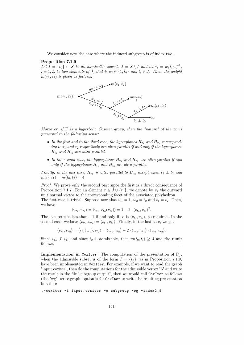
We consider now the case where the induced subgroup is of index two.
Proposition 7.1.9Let I = t0 ⊂ S be an admissible subset, J = S \ I and let τi = wi ti w
−1i ,
i = 1, 2, be two elements of J , that is wi ∈ 1, t0 and ti ∈ J . Then, the weightm(τ1, τ2) is given as follows:
Moreover, if Γ is a hyperbolic Coxeter group, then the "nature" of the ∞ ispreserved in the following sense:
• In the first and in the third case, the hyperplanes Hτ1 and Hτ2 correspond-ing to τ1 and τ2 respectively are ultra-parallel if and only if the hyperplanesHt1 and Ht2 are ultra-parallel.
• In the second case, the hyperplanes Hτ1 and Hτ2 are ultra-parallel if andonly if the hyperplanes Ht1 and Ht0 are ultra-parallel.
Finally, in the last case, Hτ1 is ultra-parallel to Hτ2 except when t1 ⊥ t2 andm(t0, t1) = m(t0, t2) = 4.
Proof. We prove only the second part since the first is a direct consequence ofProposition 7.1.7. For an element τ ∈ J ∪ t0, we denote by vτ the outwardunit normal vector to the corresponding facet of the associated polyhedron.The first case is trivial. Suppose now that w1 = 1, w2 = t0 and t1 = t2. Then,we have
〈vτ1 , vτ2〉 = 〈vt1 , rt0(vt2)〉 = 1− 2 · 〈vt0 , vt1〉2.
The last term is less than −1 if and only if so is 〈vt0 , vt1〉, as required. In thesecond case, we have 〈vτ1 , vτ2〉 = 〈vt1 , vt2〉. Finally, in the last case, we get
〈vτ1 , vτ2〉 = 〈rt0(vt1), vt2〉 = 〈vt1 , vt2〉 − 2 · 〈vt0 , vt1〉 · 〈vt0 , vt2〉.
Since vt0 6⊥ vti and since t0 is admissible, then m(t0, ti) ≥ 4 and the resultfollows.
Implementation in CoxIter The computation of the presentation of ΓJ ,when the admissible subset is of the form I = t0, as in Proposition 7.1.9,have been implemented in CoxIter. For example, if we want to read the graph"input.coxiter", then do the computations for the admissible vertex "5" and writethe result in the file "subgroup.output", then we would call CoxIter as follows(the "wg", write graph, option is for CoxIter to write the resulting presentationin a file):./ coxiter -i input. coxiter -o subgroup -wg -index2 5
151
7.2 An infinite sequence
The aim of this section is to present the construction of an infinite sequence ofindex two subgroups in a Coxeter group (Γ, S). In what follows, when consid-ering an element τ = w tw−1 ∈ J , with t ∈ J , it will be assumed that t doesnot commute with w.
Proposition 7.2.1Let (W0, S0) be a Coxeter system. If s0 and t0 are two admissible elementsof S with m(s0, t0) = ∞, then there exists an infinite sequence W of groupsW0 ≥W1 ≥W2 ≥ . . . where each Wi+1 is of index two in Wi.
Proof. For n ≥ 1 define tn = tn−1s0tn−1 =(t0s0)2n−1 t0. We construct a
subgroup W1 of W0 as above:
I1 := t0, J1 := S \ I1, J1 := J1 ∪ t0 · J1 · t0, W1 = 〈J1〉.
We want to show that t1 and s0 are admissible in J1. Let t = w · t · w, withwith w ∈ 1, t0 and t ∈ J1. If w = t0, then m(t1, t) = m(s0, t) which is even byhypothesis. If w = 1, then we getm(t1, t) = m(s0, t) orm(t1, t) =∞, dependingon the fact that t0 commutes with t or not. Hence, t1 is admissible. Similarly,s0 is admissible. Thus, we can apply again the process with
I2 := t1, J2 := S \ I2, J2 := J2 ∪ t1 · J2 · t1, W2 = 〈J2〉,
to get a subgroup W2 of W1 of index 2.Suppose now we are given a sequence (W0, S0) ≥ (W1, J1) ≥ . . . ≥ (Wn, Jn)which satisfies:
• The involutions s0 and ti are admissible in Ji for every 0 ≤ i ≤ n− 1.
• The group Wi+1 is obtained from Wi by removing ti−1 from Ii and apply-ing the process.
To see that this sequence can be extended with a subgroup (Wn+1, Jn+1) of index2 inW0, we show that s0, tn are admissible in Jn = Jn ∪ tn−1 ·Jn ·tn−1. We startwith s0. By induction hypothesis, we only need to consider the weights m(s0, t)where t ∈ tn−1·Jn·tn−1. Moreover, if t = tn−1·t·tn−1, we can suppose that t doesnot commute with tn−1, because otherwise t = t ∈ Jn. Since m(s0, t0) = ∞,then s0 does not commute with tn−1 and thus m(s0, tn−1 · t · tn−1) =∞, whichimplies that s0 is admissible. It remains to compute the weights m(tn, w · t ·w)to show that tn is admissible. By induction hypothesis, the only case to consideris when w = 1. In this, setting we get m(tn, t) =∞, since t does not commutewith tn−1. Hence, tn is admissible, as required. Thus, the sequence can beextended.
Remark 7.2.2The construction of the sequence W is purely algebraic and can be done forCoxeter groups which are not hyperbolic Coxeter groups.
152

7.2.1 Tests of CoxIter and the conjecture about Perronnumbers
Using the different graphs encoded for CoxIter (see Section 5.5), we createdmore than three thousands groups. The goal was to test the output of CoxIter(cocompactness, cofiniteness, f -vector) and that the growth rate of all thesegroups was a Perron number (see Section 5.3.5).
7.2.2 Rank of the groups of the sequence WAs before, we consider two admissible vertices t0 and s0 such thatm(t0, s0) =∞and the corresponding sequence W given by
(W0, S0) ≥ (W1, J1) ≥ (W2, J2) ≥ ...
For a vertex s ∈ Ji, we consider the neighbours of s:
N i(s) =t ∈ Ji : t 6⊥ s
.
We also considerN i∞(s) =
t ∈ Ji : m(s, t) =∞
.
Using Proposition 7.1.9, we get the following result.
Proposition 7.2.3Let n ≥ 1. The neighbours Nn(s0) of s0 in the Coxeter graph of Wn consist ofthe following:
• Nn−1(s0);
• tn−1 ·Nn−1(tn−1) · tn−1 ⊂ Nn∞(s0).
The neighbours Nn(tn) of tn consist of the following:
• Nn−1(tn−1) ⊂ Nn∞(tn);
• Nn−1(s0)
• tn−1 ·Nn−1(s0) · tn−1.
For n ≥ 0, consider the counting functions an =∣∣Nn(s0)
∣∣, bn =∣∣Nn(tn)
∣∣and cn =
∣∣Nn(s0) ∩ Nn(t0)∣∣. Using Proposition 7.2.3, we easily deduce the
following recurrence relations:
an =(an−1 − 1
)+ bn−1
bn =(an−1 + bn−1 − cn−1 − 1
)+ cn−1
= an−1 + bn−1 − 1cn = an−1 + cn−1 − 1.
Hence, we get the following proposition.
Proposition 7.2.4For an, bn and cn as above, we have for n ≥ 1
an = bn = 2n−1(a0 + b0 − 2) + 1, cn = 2n−1(a0 + b0 − 2)− b0 + c0 + 1.
153
In particular, we have
|Jn| = 2n−1(a0 + b0 − 2) + 1 + b0 − c0 + ι
= 2n−1(a0 + b0 − 2) + 1 + |J0| − a0,
where ι is the number of vertices which commute with both s0 and tn; the numberι is constant. Finally, we get
|Jn+1| − |Jn| = 2n+1(a0 + b0 − 2).
7.2.3 f-vector of the polyhedra of the sequence
We suppose now that (Γ0, S0) is a geometric Coxeter group3 (i.e. Γ0 is a discretegroup generated by finitely many reflections in hyperplanes of Sn,Hn,En) and,as before, we fix two admissible vertices t0, s0 ∈ S0 such that the correspondinghyperplanes are (ultra-)parallel. The goal is then to describe the f -vector of thepolyhedron Pn which arises after n doublings (the n here is independent of thedimension of the space).
Let F be a face of Pn−1 and denote by T ⊂ Jn−1 the corresponding spher-ical/Euclidean subgraph of the Coxeter graph Gn−1 of Γn−1. We then havethe following three possibilities when creating the doubling Pn of Pn−1 (forillustration see Figure 7.1):
F is deleted This is the case when F is contained in Htn−1 and all facets ofPn−1 going through F except Htn−1 are perpendicular to Htn−1 (edgesAB and AC and vertex A of the figure). In terms of the graph, this isequivalent to tn−1 ∈ T and T \ tn−1 ⊂ t⊥n−1.
F is duplicated This happens when F has no intersection with Htn−1 (forexample all facets of the triangle A′B′C ′ in Figure 7.1) or when F is con-tained in an hyperplane which is not perpendicular to Htn−1 (for exampleedges BB′, C,C ′ and vertices B and C). The former is equivalent totn−1 /∈ T while the later is equivalent to T \ tn−1 6⊂ t⊥n−1.
F is kept In the other cases (edge BC and vertices B and C of the Figure).Note that in this case, the corresponding figure around the face in Pn maybe different.
Hence, a face F0 of P0 can be deleted, can give rise to many faces or cancontribute only to one face in Pn. We summarize this in the next proposition.
Proposition 7.2.5Let F ⊂ P0 be a face of the first polyhedron and consider the associated subgraphT ⊂ S0. For n ≥ 1, the number of faces of the polyhedron Pn arising from Fafter n doublings is the following:
1. t0 /∈ T, s0 /∈ T :
3In this context, the bijection of Theorem 3.7.5 in Chapter 3 is still true (see for example[Vin67, Page 431] for the Euclidean case).
154

Figure 7.1 – First polyhedron of the sequence
Condition Number of facesT ⊂ t⊥0 , T ⊂ s⊥0 1
T 6⊂ t⊥0 , T 6⊂ s⊥0 2n
T 6⊂ t⊥0 , T ⊂ s⊥0 1 + 2n−1
T ⊂ t⊥0 , T 6⊂ s⊥0 2n−1
2. s0 ∈ T, t0 /∈ T :
Condition Number of facesT \ s0 ⊂ s⊥0 2
T \ s0 6⊂ s⊥0 1 + 2n−1
3. s0 /∈ T, t0 ∈ T :
Condition Number of facesT \ t0 ⊂ t⊥0 0
T \ t0 6⊂ t⊥0 2n−1
4. s0 ∈ T, t0 ∈ T : 2 faces.
Proof. We consider all the possibilities:
1. t0 /∈ T, s0 /∈ T
(a) T ⊂ t⊥0 , T ⊂ s⊥0 : F stays the same and t1 /∈ T , T ⊂ t⊥1 . Inductively,we get tn /∈ T and T ⊂ t⊥n .
(b) T 6⊂ t⊥0 , T 6⊂ s⊥0 : The face F is duplicated and this new face F (1)
will also satisfy t1 /∈ T (1), s0 /∈ T (1) and T (1) 6⊂ t⊥1 , T(1) 6⊂ s⊥0 .
Inductively, we see that this will yield to 2n faces.
155

(c) T 6⊂ t⊥0 , T ⊂ s⊥0 : The face F is duplicated and this new face F (1)
will be such that T (1) ⊂ t⊥1 and T (1) ⊂ N1∞(s0). Hence, the new
face F (1) won’t be duplicated during the second doubling but will beduplicated during each doubling after (see 1.(d)).
(d) T ⊂ t⊥0 , T 6⊂ s⊥0 : We have T 6⊂ t⊥1 and T 6⊂ s⊥0 . Hence, this faceis not duplicated during the first doubling but is during all the nextdoublings.
2. s0 ∈ T, t0 /∈ T : The face is duplicated into F (1) ⊂ Ht1 .
(a) T \s0 ⊂ s⊥0 : The new face F (1) is not duplicated nor removed afterthis first step.
(b) T \s0 6⊂ s⊥0 : F (1) is not duplicated during the second doubling butis afterwards.
3. s0 /∈ T, t0 ∈ T
(a) T \ t0 ⊂ t⊥0 : The face is removed.(b) T \ t0 6⊂ t⊥0 : Is not duplicated during the first doubling but is
afterwards.
4. We have F ⊂ Htn for for every n.
Remark 7.2.6In all cases except 3(b), the type of the graph corresponding to the face F ispreserved. In the latter case, the corresponding graph GT is modified accordingto Proposition 7.1.9 once and then remains unchanged.
Example 7.2.7We consider again the family of cocompact Coxeter prisms Γm := Γ3
4,m (seeExample 4.4.3) and we choose s0, t0 as in Figure 7.2. The spherical subgraphs
Figure 7.2 – The family of prisms Γm0 := Γ34,m
of GΓm0 together with their multiplicities are the following:
5 ∗A1 1 ∗G(m)2 1 ∗G(4)
2
1 ∗A2 6 ∗A1 ×A1 1 ∗B3
2 ∗A1 ×G(m)2 2 ∗A1 ×G(4)
2 1 ∗A1 ×A2
1 ∗A1 ×A1 ×A1.
Using Proposition 7.2.5 and Remark 7.2.6, we compute the contribution of eachof these graphs in the graph GΓmn obtained after n doublings:
• G(m)2 : 1 ∗G(m)
2 ;
• G(4)2 : 2n−1 ∗A1 ×A1;
156

• A2: (1 + 2n−1) ∗A2;
• 6 ∗A1 ×A1: (7 + 2n−1) ∗A1 ×A1;
• B3: 2n−1 ∗A3;
• 2 ∗A1 ×G(m)2 : 2 ∗A1 ×G(m)
2 ;
• A1 ×G(4)2 : 2n−1 ∗A1 ×A1 ×A1;
• A1 ×A2: 2 ∗A1 ×A2;
• A1 ×A1 ×A1 : 2 ∗A1 ×A1 ×A1.
In particular, the f -vector of Γmn is given by(2n + 6, 9 + 3 · 2n−1, 5 + 2n−1, 1
).
Implementation in CoxIter The computation of the f -vector after n dou-blings has been implemented in CoxIter. To use this feature, one should usethe option "is" (for infinite sequence), together with the name of the verticest0 and s0. For example, for the group Γ3
4,7 of the previous example, we callCoxIter as follows:./ coxiter -i ../ graphs /3-Gamma -4 ,7. coxiter -is =[4 ,5]
And the output is then the following:Reading graph:
Number of vertices : 5Dimension : 3Vertices : 1, 2, 3, 4, 5Field generated by the entries of the Gram matrix : ?
File read
Infinite sequence :f- vector after n doubling :(6, 9, 5, 1) + 2^(n -1) *(2, 3, 1, 0)Number of new hyperplanes after first doubling : 1
7.2.4 Evolution of the growth rateExample 7.2.8We continue the investigation of the properties of the groups Γmn (see Example7.2.7). Using the list of spherical subgroups, we see that the growth series isgiven by
fΓmn (x) =2(x+ 1)3 (x2 + 1
) (x2 + x+ 1
)(xm − 1)
(x+ 1) · qnm(x) ,
with
qmn (x) = −2 + 2nx+ 21+nx2 + 2x3 + 3 · 2nx3 + 2x4 + 21+nx4 + 2x5 + 2nx5
− 2x1+m − 2nx1+m − 2x2+m − 21+nx2+m − 2x3+m − 3 · 2nx3+m
− 21+nx4+m − 2nx5+m + 2x6+m,
which factors as x − 1 times a palindromic polynomial. Therefore, finding thegrowth rate τmn of Γmn is equivalent as finding the biggest positive real root
157

of qmn . Luckily for us, by Descartes’ rule of signs (see Theorem 2.6.2), each qmnhas only 3 positive real roots (and thus only one root bigger than 1).
We see that the difference qm+1n (x)− qmn (x) is equal to
(x− 1)xm+1 (2x5 − 2nx4 − 2n+1x3 − 3 · 2nx2 − 2n+1x− 2n − 2x2 − 2x− 2).
Theorem 2.6.8 implies that all the real roots of the polynomial hn(x) = 2x5 −2nx4−2n+1x3−3·2nx2−2n+1x−2n−2x2−2x−2 lie in the interval
(−2n+2, 2n+2).
Hence, we can use Sturm’s theorem (see Theorem 2.6.5) to determine the num-ber of positive real roots bigger than 1 of hn. The signs of the Sturm sequenceare the following:
αi 0 1 2 3 4 5 σ(αi)1 − − + − + + 3
2n+2 + + + − + + 2
If we denote by βn the unique root of hn bigger than 1, then we have qmn (βn) =q7n(βn) for every m ≥ 7. If q7
n(βn) ≥ 0, then τmn m is an increasing sequencebounded above by βn. On the other hand, if q7
n(βn) < 0, then τmn m is adecreasing sequence bounded below by βn. In both cases, τmn m≥7 convergesto some value τn∞ depending on n. We will see that
τmn ∈(
2n−1 + 2− 12n−1 , 2
n−1 + 2− 12n+1
), ∀n ≥ 1,m ≥ 7.
In particular, for every m ≥ 7, the ratio τmn+1τmn
goes to 2 as n goes to infinity. Weshow separately that qmn
(2n−1 + 2− 1
2n−1
)< 0 and qmn
(2n−1 + 2− 1
2n+1
)> 0.
First, remark that the last 5 monomials of qmn (x) where m arises in the powerfactors as follows when evaluated in 2n−1 + 2− 1
2n−1 :
− 2−6n−2 (22n + 2n+2 − 4) (−21−n + 2n−1 + 2
)m·(27n − 5 · 2n+7 + 9 · 22n+7 − 49 · 23n+4 + 33 · 25n+2 + 3 · 26n+3 + 128
).
Since this expression is negative and decreasing in m, we only have to show thatq7n
(2n−1 + 2− 1
2n−1
)< 0. Now, we have
q7n
(2n−1 + 2− 1
2n−1
)= −2−13n−9 (22n + 2n+1 − 4
)· pn(2),
where p(x) ∈ Z[x] is an integer polynomial whose exponents depend on n. Now,to prove that pn(2) is positive for every n ≥ 1, we replace each positive coefficientai of p by the biggest power of 2 which is smaller than ai and each negativecoefficient −ai by −2mi where mi is the smallest integer such that 2mi > ai.Hence, we find
pn(2) > −2097152− 22n+28 − 24n+30 − 26n+30 − 29n+27 − 210n+26 − 213n+23
− 214n+22 + 221n + 2n+24 + 23n+28 + 25n+30 + 27n+23 + 28n+28
+ 211n+25 + 212n+23 + 215n+17 + 216n+18 + 217n+16 + 218n+13
+ 219n+10 + 220n+5
> −2097152− 7 · 214n+22 + 220n+5,
158

which is bigger than 0 if n > 2. For n = 1 and n = 2, a direct computationshows that pn(2) > 0, as required. With the same kind of comparisons, we canshow that qmn
(2n−1 + 2− 1
2n+1
)> 0, as required.
We saw in the previous example that for a fixed m, the quotient τn+1τn
goes to2 as n goes to infinity when the considered sequence is built from one family ofKaplinskaya prisms. Next proposition relates the growth series of two successiveterms in the sequence.
Proposition 7.2.9Let (Γ0, S0) be a hyperbolic Coxeter group and let t0, s0 ∈ S0 be two admissiblevertices with m(t0, s0) =∞. Then, there exists a polynomial q ∈ Z[x] such thatthe rational expansion of the growth series fΓn of the group after n doublingscan be written
fΓn(x) = q(x)gn(x) , gn(x) ∈ Z[x].
Moreover, there exists r ∈ N such that the gn are related as follows:
gn+1(x) = (2n − 1) · xr · g(x) + g1(x)
Proof. We know from Steinberg’s formula that the growth series is given by
1f(Γn,Sn)(x) =
∑T∈Fn
(−1)|T | · xmTfT (x) ,
where Fn is the collection of subsets T of Sn such that the subgroup generatedby T is finite, and where mT is some exponent depending on the type of T(see Figure 5.3 on page 83). Since the list of spherical subgroups of Γn remainsunchanged if n ≥ 1 (see Remark 7.2.6), we can regroup terms corresponding tothe same subgroups and write
1f(Γn,Sn)(x) =
∑T∈F
(−1)|T | · xmTfT (x) · αT,n,
where F is the list of representatives of distinct finite subgroups of Γ1. Moreover,Proposition 7.2.5 implies that αT,n ∈ 1, 2, 1 + 2n−1, 2n−1, 2n. We now have
1f(Γn,Sn)(x) = gn(x)
q(x) ,
where gn(x) has constant coefficient 1, a degree independent of n, and whereq(x) is independent of n. Now, each coefficient of gn(x) splits as a sum of a termwhich is independent of n and a term which is divisible by 2n−1. Therefore, wehave
gn+1(x)− gn(x) = 2n−1 · xd · g(x),
for some positive integer r and some polynomial g ∈ Z[x] and thus
gn+1(x) = (2n − 1) · xr · g(x) + g1(x).
159

Corollary 7.2.10Consider the gn as in Proposition 7.2.9 and let r ∈ N and g ∈ Z[x] be such that
gn+1(x) = (2n − 1) · xr · g(x) + g1(x).
If there exists an index m such that the smallest positive root of gm is strictlyless than the smallest positive root of g, then
limn→∞
τn+1
τn= 2r.
As indicated above, we constructed the first terms of all possible sequences ofknown cofinite hyperbolic Coxeter groups (see all groups mentioned in Section5.5). For all these sequences (more than 500), we checked numerically that thesituation of the Corollary 7.2.10 applies; more precisely:
• we have τn+1τ −→ 2;
• often, the smallest positive root of g1 is smaller than the smallest positiveroot of g.
These experimental observations lead us to state the following.
ConjectureLet (Γ0, S0) be a hyperbolic Coxeter group and let t0, s0 ∈ S0 be two admissiblevertices with m(t0, s0) = ∞. Then, the growth rate τn of the group Γn arisingafter n doublings satisfies
limn→∞
τn+1
τn= 2.
160
CHAPTER 8Clifford algebras and isometries of (infinite
dimensional) hyperbolic spaces
Clifford algebras are unitary associative algebras which provide a way to gen-eralize complex numbers and quaternions. Moreover, by considering a certaingroup of two-by-two matrices with coefficients in a subset Γn ∪0 of a Cliffordalgebra, one gets a way to describe the group of orientation preserving isometriesof the hyperbolic n-space, i.e. we have an isomorphism
PSL(2; Γn) ∼= Isom+ Hn+2.
In low dimensions, this result gives the well know isomorphisms
PSL(2;R) ∼= Isom+ H2, PSL(2;C) ∼= Isom+ H3.
The construction of the group PSL(2; Γn), its basic properties and its actionby isometries on the hyperbolic (n+ 2)-space via Poincaré extension have beenextensively studied over the last decades (see [Ahl85] and [Wat93] for example).
The goal of this chapter is to explain how we can generalize the constructionof the group PSL(2; Γn) to the infinite-dimensional setting. For a given infinite-dimensional Hilbert space H , we will be able to give a description of the groupMob∗(H ) (see Definition 2.7.17) in terms of Clifford matrices. Then, we willsee that this group induces isometries of the associated upper half-space modelUH (see Section 3.2.1). Other authors studied Clifford matrices induced Möbiustransformations in the infinite-dimensional setting (see [Li11] and [Fru91], forexample) but they considered only the case H = `2. Our approach, which ismore canonical, allows to consider any Hilbert space and its induced hyperbolicspace. In this way, we are able to use the work of [Das12].
In the first section, we will present the construction of the Clifford algebraassociated to any quadratic space (V, q) and study its basic properties. In thesecond part, we will determine under which conditions a two-by-two matrix withcoefficients in the Clifford group induces a bijection of the ambient space andsee how the usual transformations (reflections, translations, sphere inversions,etc.) can be rewritten by means of Clifford matrices. Most results of thispart are adaptations of Waterman’s results to the infinite-dimensional setting.Finally, we will show that Clifford matrices induce isometries of the associatedhyperbolic space and discuss the classification of the isometries in this setting.
161

In this chapter, any field will be supposed to have characteristic differentfrom 2. Moreover, we will denote invertible elements of a ring R by R× insteadof R∗ in order to avoid confusion with the involution ∗ of the Clifford algebra.
8.1 Construction and basic properties
8.1.1 Clifford algebrasLet (V, q) be a quadratic space defined over some field K. A Clifford algebraassociated to (V, q) is a unitary associative algebra over K denoted by Cl(V, q),together with a K-linear map i : V −→ Cl(V, q) which satisfies the followingtwo properties:
• Clifford identityWe have i(v)2 = −q(v) · 1Cl(V,q) for every v ∈ V .
• Universal propertyIf A is another unitary associative K-algebra together with a K-linearfunction iA : V −→ A such that iA(v)2 = −q(v) · 1A for every v ∈ V , thenthere exists a unique morphism of K-algebras ψ : Cl(V, f) −→ A suchthat the following diagram commutes:
ViA //
i
A
Cl(V, q)ψ
;;
The universal property implies that if the algebra Cl(V, q) exists, then it isunique up to isomorphism. In fact, the Clifford algebra can be constructedexplicitly as follows. We start with the tensor algebra T (V ) =
⊕i∈N0
V ⊗n,where V ⊗n = V ⊗ . . .⊗V , n times, and V ⊗0 = K. Then, we consider the ideal Iin T (V ) generated by the elements v2 +q(v). It follows that the quotient T (V )/Isatisfies the universal property, as required. Thus, we have Cl(V, q) = T (V )/I.Since the composition
V // T (V ) // // T (V )/I
is injective, we will write v instead of i(v) for the image of a vector in Cl(V, q).Moreover, when working in Cl(V, f) we will write the product a · b instead ofa⊗ b.
Let vii∈I be an algebraic basis of V (see Remark 2.7.6) and consider somewell-order on I. A multi-index I will denote a finite ordered subset of I. IfI = (i1, . . . , ik), we will say that I has length k and write |I| = k. Any elementa ∈ Cl(V, q) can be written as a =
∑I aI · vI , where the finite sum is taken over
multi-indices I = (i1, . . . , ik), aI ∈ K, and vI := vi1 · . . . ·vik , with the additionalconvention that v∅ := 1 = 1K .
The natural N0-grading on the tensor algebra T (V ) induces a(Z/2Z
)-grading
on Cl(V, f) which is compatible with the algebra structure. In other words, thevector space
Cl0(V, f) := spanKvi1 · . . . · vik : 1 ≤ i1 < i2 < . . . < ik ≤ n, k even
162
is a sub-algebra of Cl(V, f) called the even part of Cl(V, f). More canonically,Cl0(V, f) is the image of
⊕i∈N0
V ⊗2i by the corresponding quotient map.
Notice, that Cl(V, q), when viewed as a vector space, also has a Z-grading.However, this grading is not compatible with the algebra structure.
8.1.1.1 Functoriality and three involutions
If (V ′, q′) is another quadratic space over K and φ : V −→ V ′ is a morphismof quadratic spaces (i.e. a linear map preserving the quadratic forms), then thecomposition iv′ φ satisfies the condition of the universal property, which meansthat there exists a morphism of K-algebras, again denoted φ, from Cl(V, q) toCl(V ′, q′). With the explicit construction of the Clifford algebra, the map φ canbe described as follows:
φ : Cl(V, q) −→ Cl(V ′, q′)v1 · . . . · vm 7−→ φ(v1) · . . . · φ(vm).
Therefore, Cl is a functor from the category of quadratic spaces over a field Kto the category of unitary associative algebras over K.
The automorphism of (V, q) which sends a vector v to −v then induces anautomorphism ′ : Cl(V, q) −→ Cl(V, q) which sends an element v1 · . . . · vm to(−1)m · v1 · . . . · vm. The inclusion of Cl(V, q) in its opposite algebra Cl(V, q)op
gives rise to an anti-automorphism ∗ : Cl(V, q) −→ Cl(V, q) which sends anelement v1 · . . . ·vm to vm · . . . ·v1. Since these two maps commute, we can definethe following anti-automorphism
: Cl(V, q) −→ Cl(V, q)a 7−→ a = (a′)∗ = (a∗)′.
Example 8.1.1 (Standard Clifford algebra)For a field K of characteristic different from two, and for n ∈ N0, we let Vn =Kn, with the convention that K0 is the null space 0. Any orthonormal basise1, . . . , en of Vn gives rise to the diagonal quadratic form qn = 〈1, . . . , 1〉. Inthe Clifford algebra Cl(Vn, qn), we have the identities e2
i = −1 and eiej = −ejei,when i 6= j. Moreover, it is easy to see that
ei1 · . . . · eik : 1 ≤ i1 < i2 < . . . < ik ≤ n
is a K-basis of Cl(Vn, qn) and in particular dimK Cl(Vn, qn) = 2dimK Vn = 2n.We will denote this Clifford algebra by Cln(K), or Cln if K = R. For n = 0, 1and 2 we get successively Cln = R, C and H, with the standard basis 1, 1, iand 1, i, j, ij. Moreover, the anti-automorphism coincides with the usualconjugation in C and H.
8.1.1.2 Center of the algebra
Proposition 8.1.2 (Center of Cl, finite-dimensional case)Let (V, q) be an n-dimensional quadratic space over K with orthogonal basisv1, . . . , vn. Then, the center of Cl(V, q) is K if n is even, and it equalsspan1, v1 · . . . · vn if n is odd.
163

Proof. First, we remark that the following two equalities hold for every multi-index I:
vj · vI = (−1)|I| · vI · vj , j /∈ Ivj · vI = (−1)|I|+1 · vI · vj , j ∈ I.
(8.1)
Let a ∈ Cl(V, q) and write a =∑aI ·vI , where all the multi-indices I are distinct
and totally ordered, that is I = (i1, . . . , ik) for some 1 ≤ i1 < i2 < . . . < ik ≤ n.If J is any multi-index, then we have vI · vJ ∈ R · vI∆J , where I∆J denotes thesymmetric difference between I and J , that is I∆J = (I \ J) ∪ (J \ I). SinceI∆J = I ′∆J implies I = I ′, it follows that a is in the center of the Cliffordalgebra if and only if every vI such that aI 6= 0 is also in the center. Moreover,this last condition is equivalent to vI · vj = vj · vI for every 1 ≤ j ≤ n. Weconclude using equations (8.1).
Proposition 8.1.3 (Center of Cl, infinite-dimensional case)Let (V, ‖·‖) be an infinite-dimensional Hilbert space, let λ ∈ R\0 and considerthe quadratic form q : V −→ R defined by q(v) = λ · ‖v‖2. Then, the center ofCl(V, q) is R.
Proof. First, we pick a Hilbert orthonormal basis eii∈I of V (see Definition2.7.2). We thus have the following relations:
e2i = −λ, ei · ej = −ej · ei, ∀i 6= j ∈ I.
We know (see Proposition 2.7.14) that the set of products
ei1 ⊗ . . .⊗ eik , i1, . . . , ik ∈ I
is an orthonormal Hilbert basis of V ⊗k (see Definition 2.7.13). Hence, theclosure of the linear span of the family of vectors
C =ei1 · . . . · eik : k ∈ N, i1, . . . , ik ∈ I
is Cl(V, q). Let x ∈ Z(Cl(V, q)
)and write
x =∑J∈J
aJeJ , aJ 6= 0,∀J ∈ J ,
where eJJ∈J is a finite or countable subset of C consisting of linearly indepen-dent vectors. If x /∈ R, then there exists a non-empty J ∈ J such that aJ 6= 0.Moreover, we must have eieJ = eJei for every i ∈ I (see proof of Proposition8.1.2). If |J | is odd this is possible only for i ∈ J , and only for i /∈ J if |J | iseven (see equations (8.1) of Proposition 8.1.2). Therefore, we must have x ∈ R,as required.
8.1.1.3 The Clifford algebra as a quadratic space
The vector space Cl(V, q) has a natural grading given by the one on the tensoralgebra and the projection T (V ) −→ T (V )0 = K gives rise to the linear map
< : Cl(V, q) −→ K
x 7−→ x0.
164

This map yields a quadratic form q on Cl(V, q) and its associated bilinear form
q : Cl(V, q) −→ K B : Cl(V, q)× Cl(V, q) −→ K
x 7−→ <(xx) (x, y) 7−→ 12<(xy + yx) = <(xy).
We note that the quadratic form q, when restricted to V , agrees with the initialone. Moreover, if φ : (V, q) −→ (V ′, q′) is a morphism of quadratic spaces,then the induced map φ : Cl(V, q) −→ Cl(V ′, q′) preserves the bilinear forms onCl(V, q) and Cl(V ′, q′).Proposition 8.1.4Let x1, . . . , xk, x, y ∈ K ⊕ V , v, v ∈ V , α, α ∈ K and z ∈ Cl(V, q). Then, wehave the following properties:(i) B(α+ v, α+ v) = αα+B(v, v);
(ii) q(α+ v) = α2 + q(v);
(iii) q(x1 · . . . · xk) =∏ki=1 q(xi);
(iv) q(xz) = q(x) · q(z);
(v) xx = q(x);
(vi) xy + yx = 2 · b(x, y).Proof. For the sake of clarity, we will write q for the quadratic form defined onV (respectively b for its associated bilinear form) and Q for the one defined onCl(V, q) (respectively B for its associated bilinear form).
(i) We will prove the equality B(α+v, α+ v) = αα+ b(v, v). First we remarkthat by definition of b, we have
b(v, v) = 12(q(v + v)− q(v)− q(v)
)= 1
2(−(v + v)2 + v2 + v2)
= −12(vv + vv) = −<(vv).
Then, we get
B(α+ v, α+ v) = < ((α+ v)(α+ v)) = < (αα− αv + αv − vv)= αα−< (vv) = αα+ b(v, v),
as required.
(ii) Follows directly from (i).
(iii) We write x1 = α1 + v1 and we get
Q(x1x2) = <(x2x1x1x2
)= <
(x2(α2
1 − v21)x2
)= Q(x1) · <
(x2x2
)= Q(x1) ·Q(x2).
(iv)-(vi) Follow easily from direct computations.
Remark 8.1.5The points (v) and (vi) are not true for arbitrary elements of Cl(V, q). Forexample, xx may fail to be an element of K.
165

8.1.2 Vectors and the Clifford groupDefinition 8.1.6 (Vectors)The elements of the subspace K ⊕ V will be called vectors. We will denote theset K ⊕ V ∪ ∞ by Vext, and its elements will be called extended vectors.
As we saw before, the quadratic form is multiplicative when restricted tovectors. Moreover, vectors lead to the construction of a multiplicative subgroupof Cl(V, q) called the Clifford group as follows.
Proposition 8.1.7Let x ∈ Cl(V, q) be a product of vectors. Then, x is invertible if and only ifq(x) 6= 0, and its inverse is then given by x−1 = 1
q(x)x. In particular, theinverse of a product of vectors is again a product of vectors.
Definition 8.1.8 (Clifford group)The group of all products of invertible vectors is called the Clifford group ofCl(V, q) and is denoted by ΓCl(V,q), or just by Γ. For the standard Cliffordalgebras (see Example 8.1.1), we will denote the Clifford group by Γn(K) orjust Γn if K = R.
Remark 8.1.9Later on we will restrict ourselves to an anisotropic quadratic form, so that theClifford group consists of all products of non-zero vectors.
Example 8.1.10We have Γ0 = R×, Γ1 = C× and Γ2 = H×. In higher dimensions, it is not truethat Γn = Cln \0.
Any invertible element x ∈ Cl(V, q) gives rise to a linear automorphism
ρx : Cl(V, q) −→ Cl(V, q)
y 7−→ xyx′−1.
Lemma 8.1.11For any x ∈ Γ, then ρx ∈ O(K ⊕ V, q).
Proof. First, we prove that ρx(y) ∈ K ⊕ V for any y ∈ K ⊕ V . If x is a vector,then the equality xy+yx = 2 · b(x, y) implies xyx = 2 · b(x, y)x−q(x)y and thus
xyx∗ = xyx = 2 · b(x, y)x− q(x)y ∈ K ⊕ V.
Hence, we have xyx′−1 ∈ K ⊕V . Now, proceed by induction for finite productsof vectors. Finally, we obtain:
q(ρx(y)
)= xyx′
−1 · xyx′−1 = xy q(x−1) y x
= 1q(x)xyy x = q(y).
Remark 8.1.12The map ρx corresponds to Rx R1, where Rx, respectively R1, denotes the
166
reflection with respect to the hyperplane perpendicular to x, respectively to 1.Indeed, we see that the two reflections are given by
Rx(y) = y − 2b(x, y)q(x) · x
R1(y) = y − 2<(y)1 1 = −y.
Then, an easy computation gives Rx R1 = ρx.Lemma 8.1.13If a and b are two elements of Γ, then
ab−1 ∈ K ⊕ V ⇔ a∗b ∈ K ⊕ V.
Proof. We have
ab−1 ∈ K ⊕ V ⇔ b∗−1a∗ ∈ K ⊕ V
⇔ ρb∗(b∗−1a∗
)∈ K ⊕ V
⇔ a∗b1q(b) ∈ K ⊕ V.
Lemma 8.1.14For x, y ∈ Γ, then we have <(x · y · x−1) = <y.Proof. First, notice that if the claim is true when x is a vector, then the generalcase follows by induction. Hence, we suppose that we have x = x0 +xv ∈ K⊕Vwith x0 ∈ K and xv ∈ V . We also write y =
∑I yI · vI , where yI ∈ K are
the components of y with respect to the basis vI of Cl(V, q). Now, using theK-linearity of <, we get
<(x · y · x−1) =∑I
yI · <(x · vI · x−1)
=∑I
yI · <(
(x0 + xv) · vI ·1
q(x) (x0 − xv))
= <(y) + 1q(x)
∑I 6=∅
<(x2
0 · vI − x0 · vI xv + x0 · xv vI − xv vI xv)
= <(y) + 1q(x)
∑I 6=∅
< (−x0 · vI xv + x0 · xv vI − xv vI xv) .
If |I| = 1, then <(x0 · vI xv) = <(x0 · xv vI) and <(xv vI xv) = 0. On the otherhand, if |I| ≥ 2, then all three terms are zero. Therefore, we have <(x ·y ·x−1) =<(y), as required.
8.2 Clifford matrices and their action on the am-bient space
Consider g =(a bc d
)∈ Mat(2; ΓCl(V,q) ∪ 0). We want to determine the
conditions under which g induces a bijection g : Vext −→ Vext (see Definition
167
8.1.6) via x 7−→ (ax+ b)(cx+ d)−1. First, we remark that we must have
g(0), g(∞), g−1(0), g−1(∞) ∈ Vext,
which gives the following.
Proposition 8.2.1
If g =(a bc d
)∈ Mat(2; ΓCl(V,q)∪0) induces a bijection Vext −→ Vext, then
we must havebd−1, ac−1,−a−1b,−c−1d ∈ Vext
or equivalently (see Lemma 8.1.13)
b∗d, a∗c, ab∗, cd∗ ∈ Vext.
Another obvious condition is that cx+d has to be either zero or invertible (seeProposition 8.1.7). This is automatically fulfilled if V is a normed vector spaceand q is a non-zero multiple of the norm or, more generally, if q is anisotropic.Also, we don’t want ax + b and cx + d to be zero at the same time. If thishappens, then a and c must be different from zero which gives a−1b = c−1d andthus
ad∗ = a(b∗a−1∗c∗
)= a
(a−1b
)∗c∗
8.2.1= aa−1bc∗ = bc∗.
Definition 8.2.2 (Determinant of a Clifford matrix)
Let g =(a bc d
)∈ Mat(2; ΓCl(V,q) ∪ 0). The determinant of g is ∆(g) =
ad∗ − bc∗.
Proposition 8.2.3
If g =(a bc d
)∈ Mat(2; ΓCl(V,q)∪0) induces a bijection Vext −→ Vext, then
we must have ∆(g) 6= 0.
Proposition 8.2.4The composition of applications is induced by the composition of matrices.
Proof. For g =(a bc d
), g =
(α βγ δ
)∈ Mat(2; ΓCl(V,q) ∪ 0), we com-
pute:
g(g(x)
)=(a(αx+ β)(γx+ δ)−1 + b
)(c(αx+ β)(γx+ δ)−1 + d
)−1
=(a(αx+ β) + b(γx+ δ)
)(γx+ δ)−1(c(αx+ β)(γx+ δ)−1 + d
)−1
=(a(αx+ β) + b(γx+ δ)
)((c(αx+ β)(γx+ δ)−1 + d
)(γx+ δ)
)−1
=((aα+ bγ)x+ aβ + bδ
)(c(αx+ β) + d(γx+ δ)
)−1
=((aα+ bγ)x+ (aβ + bδ)
)((cα+ dγ)x+ (cβ + dδ)
)−1
= (g · g)(x).
168

In general, ∆ is not a multiplicative function from the group of matricesinducing a bijection Vext −→ Vext to Cl(V, q). However, we have the followingresult.
Proposition 8.2.5
Let g =(a bc d
), g =
(α βγ δ
)∈ Mat(2; ΓCl(V,q) ∪ 0) inducing bijections
such that ∆(g) = ∆(g)∗. Then, ∆(g · g) = ∆(g) ·∆(g).
Proof. We compute
∆(gg) = aαβ∗c∗ + aαδ∗d∗ + bγβ∗c∗ + bγδ∗d∗
− aβγ∗d∗ − aβα∗c∗ − bδγ∗d∗ − bδα∗c∗
8.2.1= aαδ∗d∗ + bγβ∗c∗ − aβγ∗d∗ − bδα∗c∗
= a∆(g) d∗ − b∆(g)∗ c∗
= ∆(g) ·∆(g).
Proposition 8.2.6
Let g =(a bc d
)∈ Mat(2; ΓCl(V,q) ∪ 0). Then, g induces the identity if and
only if g is a diagonal matrix with a = d ∈ Z(Cl(V, q))×.
Proof. Suppose that g induces the identity. Substituting x = 0,∞ and 1 givesb = 0, c = 0 and a = d. Now, we have ax = xa for every x ∈ V which meansax = xa for every x ∈ Cl(V, q), as required. The converse is obvious.
We want to determine the inverse of the matrix g =(a bc d
). If we write
y = (ax+b)(cx+d)−1, then we have (yc−a)x = b−yd. Except when y = ac−1,which happens when x =∞, the term (yc− a) is invertible, which yields
x = (yc− a)−1(b− yd) = (d∗y − b∗) (−c∗y + a∗)−1.
This motivates to look at g∗ =(
d∗ −b∗−c∗ a∗
), and we find the products
g · g∗ =(
∆(g) 00 ∆(g)∗
)g∗ · g =
(∆(g∗)
00 ∆
(g∗)∗ ) . (8.2)
A necessary condition for the invertibility of the map induced by g is that∆(g) ∈ Z(Cl(V, q))×, ∆(g) = ∆(g)∗ and ∆(g∗) = ∆(g∗)∗.
Definition 8.2.7 (Clifford matrices)We define GL(ΓCl(V,q)), or just GL(Γ), to be the set of matrices of the form
g =(a bc d
)∈ Mat(2; Cl(V, q)) which satisfy the following conditions:
• a, b, c, d ∈ Γ ∪ 0;
169
• ∆(g) = ad∗ − bc∗ ∈ K×;
• ab∗, cd∗, c∗a, d∗b ∈ K ⊕ V .
We also define SL(Γ) = g ∈ GL(Γ) : ∆(g) = 1 and PSL(Γ) = SL(Γ)/±I.
Remarks 8.2.8 • Using Theorem 8.2.11 below, we will see that GL(Γ) is agroup.
• If ∆(g),∆(g∗) ∈ K, then equations (8.2) imply that g = ∆(g) · g∗−1 andg∗ = ∆(g∗) · g−1 which gives ∆(g) = ∆(g∗).
• Scaling all the coefficients of a matrix by an element of K× does notchange the induced application. Therefore, if K = R, we can supposethat ∆(g) = ±1.
Definition 8.2.9 (Trace of a matrix)
Let g ∈(a bc d
)∈ Mat(2; ΓCl(V,q) ∪ 0). Then, the trace of g, denoted by
Tr g, is defined to be Tr(g) = a+ d∗.
Following [Li11], we also have the following definition.
Definition 8.2.10 (Vectorial element)
A non-trivial Clifford matrix g ∈(a bc d
)∈ GL(Γ) is called vectorial if b∗ = b,
c∗ = c and Tr g ∈ R.
8.2.1 Algebraic characterizationFrom now on, we suppose that the quadratic form q is anisotropic. In thissetting, every non-zero vector v ∈ V is invertible and in particular, Γ consistsof all products of non-zero vectors. We also request that the only matricesinducing the identity map are multiples of the identity matrix by an element ofK×. This is the case in the following two situations:
1. The center of the Clifford algebra is trivial.This happens when dimK V is even (see Proposition 8.1.2) or whenK = R,V is an infinite-dimensional Hilbert space with norm ‖ · ‖2 and q(v) =λ · ‖v‖2 for some fixed λ ∈ R× (see Proposition 8.1.3).
2. The Clifford algebra is a standard Clifford algebra (see Example 8.1.1).Then, a matrix g ∈ Mat(2; Γn(K) ∪ 0) induces a map on both Kn
extand Kn+1
ext . Hence, we can consider matrices g ∈ Mat(2,Cl(Vn, qn)) whichinduce bijections on Kn
ext −→ Knext and Kn+1
ext −→ Kn+1ext . If such a matrix
induces the identity on both Knext and Kn+1
ext , then g is the multiple of theidentity matrix by an element of K× (see Proposition 8.1.3). This secondinstance is used by [Ahl85] and [Wat93].
Theorem 8.2.11Let (V, q) be an anisotropic quadratic space over a field K such that the center of
the Clifford algebra Cl(V, q) is K, and let g =(a bc d
)∈ Mat(2; ΓCl(V,q)∪0).
Then, g induces a bijection on Vext if and only if g ∈ GL(Γ).
170
Theorem 8.2.12Let n ∈ N0 and g =
(a bc d
)∈ Mat(2; Γn(K) ∪ 0). Then, g induces a
bijection on Knext and Kn+1
ext if and only if g ∈ GL(Γ).
Proof. We already saw that these algebraic conditions are necessary.Suppose now that g ∈ GL(Γ). First, we want to check whether the expression(cx+d)−1 actually makes sense. If c = 0, then d is non-zero and thus is invertible.On the other hand, if c 6= 0, then we have cx+d = c(x+c−1d), where the secondterm is either zero or an element of K ⊕V (and thus invertible). We now provethat the image of g lies in Vext. For x, y ∈ K ⊕ V , a direct computation gives
(yc∗ + d∗)(ax+ b)− (ya∗ + b∗)(cx+ d) = −y ·∆(g) + ∆(g−1)x= ∆(g) (x− y)
which leads to
gx− (gy)∗ = ∆(g) (yc∗ + d∗)−1(x− y)(cx+ d)−1. (8.3)
Letting y = 0 gives
(gx− g0)−1 = ∆(g) ·(cd∗ + dx−1d∗
),
which is a vector (or∞) by Proposition 8.2.1 and Lemma 8.1.11. Hence, gx−g0is a vector (or∞) and so is gx, as required. Now, equation (8.3) can be rewritten
gx− gy = ∆(g) (yc∗ + d∗)−1(x− y)(cx+ d)−1,
which implies the injectivity of g. Now, the matrix g∗ =(
d∗ −b∗−c∗ a∗
)satisfies
the algebraic conditions which insure that g∗ induces a map from Vext to Vext,and this map is the inverse to the one induced by g.
8.2.2 Typical transformations of a Hilbert spaceIn this section, we suppose that V is a real Hilbert space and q = λ · ‖ · ‖2, forsome λ ∈ R×. We express the typical transformations of the space V by meansof Clifford matrices as follows. First, we write the inversion ι with respect tothe unit sphere S(0, 1):
ι =(
0 −λ1 0
)∈ GL(Γ).
The inversion with respect to the sphere with center a ∈ V and radius r, iswritten
ιS(a,r) = f ι f−1, f =(r a0 1
)∈ GL(Γ).
The reflection with respect to the hyperplane P (a, α) = v ∈ V : 〈v, a〉 = α isgiven by:
• For α 6= 0: f ι f−1, with f = ι ϕ, where
ϕ(x) =∥∥∥ a2α∥∥∥ · x+ a
2α.
171

• For α = 0: g ι g with g = ψ ι ϕ, where
ϕ(x) = ‖a‖ · x+ a, ψ(x) = x− a
2 · ‖a‖2 .
We know present a lemma which will have many important consequences.Lemma 8.2.13Any Clifford matrix g induces an application g : Vext −→ Vext which is a com-position of the following transformations:
translation Tµ =(
1 µ0 1
)x 7−→ x+ µ, µ ∈ K ⊕ V
inversion ι =(
0 −λ1 0
)x 7−→ −λx−1
dilatation Dr =(r 00 1/r
)x 7−→ r2 x, r ∈ R×+
orthogonal Sa =(a 00 a′
)x 7−→ axa∗, a ∈ Γ, Q(a) = 1
reflection R =(
1 00 −1
)x 7−→ −x.
In the sequel, we use the function
ε : R× −→ 0, 1, x 7−→
0 if x > 01 otherwise.
Remarks 8.2.14 (i) If Q(a) 6= 1, then the transformation x 7−→ axa∗ can bewritten as follows:
Sa = D√|Q(a)| · Sa/Q(a) ·Rε(Q(a)).
Hence, we can assume without loss of generality that Q(a) is equal to 1.
(ii) If a is a vector, then Sa corresponds to the map ρa, which consists ofthe reflection with respect to the hyperplane perpendicular to 1, followedby the reflection with respect to the hyperplane perpendicular to a (seeRemark 8.1.12).
(iii) In particular, the lemma implies that every Clifford matrix induced mapis in Mob∗. The reverse inclusion follows from (ii).
(iv) If x ∈ V , then ι(x) = x‖x‖2 . More generally, if x = α + v with v ∈ V and
α ∈ R, thenι(x) = −λ
Q(α+ v)α+ λ
Q(α+ v)v.
Proof. We distinguish the cases where c = 0 and c 6= 0.• Let c = 0. In this setting, we have
gx = 1∆(g)axa
∗ + bd−1,
that is,
g = Tbd−1 (D√
|∆(g)|−1 Rε(∆(g))
)︸ ︷︷ ︸
1/∆(g)
(D√|Q(a)| Sa/Q(a) Rε(Q(a))
)︸ ︷︷ ︸
Sa
.
172

• Let c 6= 0. First, we see that b = ac−1d−∆(g) · c∗−1. Then, we compute
gx =(ac−1(cx+ d)−∆(g) · c∗−1
)(cx+ d)−1
= ac−1 −∆(g) · c∗−1(x+ c−1d)−1c−1.
Furthermore, we can write
x−1 = Rε(λ) D1/√|λ| ι(x).
Since ac−1, c−1d ∈ V , we can combine the different transformations above,and conclude.
Using the decomposition provided by the Lemma 8.2.13, we get the followingresult.
Proposition 8.2.15Let W be a subspace of the vector space V and let g : Wext −→ Wext be amap induced by a Clifford matrix. Then, the trivial extension g : Vext −→ Vextcorresponds to the Poincaré extension of g (see Definition 3.2.4).
Since the group of Möbius transformations of Rn+1 is generated by reflectionsin spheres and hyperplanes, we have the following corollary.
Corollary 8.2.16The map which sends a Clifford matrix g ∈ GL(Γn) to the induced map g :Rn+1
ext −→ Rn+1ext yields a group isomorphism GL(Γn)/R× ∼= Mob(Rn+1).
The Lemma 8.2.13, together with Remark 8.2.14, also give the analogue ofthe Corollary 8.2.16 in the infinite-dimensional setting.
Proposition 8.2.17Let H be a Hilbert space, of finite or infinite dimension, and consider a codi-mension one subspace H ′ of H . If we let Γ′ be the Clifford group associatedto Cl(H ′, q′), where q′ is the restriction of ‖ · ‖2 to H ′, then we get
GL(Γ′)/R∗ ∼= Mob∗(H ).
Themotto behind the result is the following: any map coming from a Cliffordmatrix can be written as the Poincaré extension of a map coming from a Cliffordmatrix g ∈ GL(ΓVf ), where Vf is a finite-dimensional subspace of H . This willbe made more precise by Proposition 8.2.18 below. Before that, let us recall thedefinition of a direct system and a direct limit of groups1. The starting point isa directed, or filtered, set (I,≤). It means that ≤ is a preorder on I such thatany pair of elements i, j ∈ I has an upper bound (i.e. there exists k ∈ I suchthat i ≤ k and j ≤ k). Then, we consider a collection of groups Gii∈I andwe suppose that for every i ≤ j we have a homomorphism ϕi,j : Gi −→ Gj .Finally, it is required that the morphisms ϕi,j enjoy the following properties:
• For every i ∈ I, we have ϕi,i = idGi .1More generally, the notion of direct limit can be defined using a universal property in any
category.
173
• For every i ≤ j ≤ k in I, we have ϕj,k ϕi,j = ϕi,k.
The collection (Gi, ϕi,j) is called a direct system.Now, we consider on the disjoint union
⊔iGi the equivalence relation ∼
defined as follows: for g ∈ Gi and h ∈ Gj , we have g ∼ h if and only ifthere exists k ∈ I such that ϕi,k(g) = ϕj,k(h) in Gk. We can endow the setlim−→i∈I Gi :=
⊔i∈I Gi/∼ with a group structure as follows: for g ∈ Gi and
h ∈ Gj , we consider an upper bound k of i and j and we define
[g] · [h] :=[ϕi,k(g) · ϕj,k(h)
],
where [−] denotes the equivalence class of an element. It is easily shown that thisdefinition is independent of the choice of the upper bound and indeed defines agroup structure on lim−→i∈I Gi. The group lim−→i∈I Gi is called the direct limit ofthe system
(Gi, ϕi,j
). A typical direct system is given by the lattice of finite-
dimensional subspaces of a given vector space and the morphisms are just theinclusions. We are now ready to present the proposition.
Proposition 8.2.18For (H , ‖ · ‖) a Hilbert space, we denote by V the set of all finite-dimensionalsubspaces of H . For every V ∈ V, we denote by GL(ΓV ) the group of Cliffordmatrices corresponding to the quadratic space (V, ‖ · ‖2). Then, we have
lim−→V ∈V
GL(ΓV ) ∼= GL(Γ),
where GL(Γ) is the group of Clifford matrices corresponding to (H , ‖ · ‖2).
Proof. First, we notice that the direct limit is well-defined: the inclusion of finitesubspaces of H induces an order on V and the upper bound of two elementsin V is given by the direct sum. Moreover, if V ⊂ V ′ are two elements of V,then the map ϕV,V ′ : GL(ΓV ) −→ GL(ΓV ′) is given by the Poincaré extension.Therefore, (GL(ΓV ), ϕV,V ′) is a direct system.
Now, the collection of group homomorphisms GL(ΓV ) −→ GL(Γ) given byPoincaré extensions is compatible with the direct system, which means that weget an injective homomorphism ψ : lim−→V ∈V GL(ΓV ) −→ GL(Γ). The surjectiv-ity of ψ is given by Lemma 8.2.13.
Lemma 8.2.13 is at the basis of the following result.
Proposition 8.2.19
Let g ∈(a bc d
)∈ Mat(2; ΓCl(V,q) ∪ 0). Then, <(Tr(g)) is invariant under
conjugation by an element of GL(Γ).
Proof. Let h ∈ GL(Γ). In order to show that <(Tr(h · g · h−1)
)= <(Tr(g)), it
is sufficient to prove the equality for h = Tµ, ι,Dr, Sa and R of Lemma 8.2.13.We consider these cases separately.
• For h = Tµ: We have h =(
1 µ0 1
), for some µ ∈ K ⊕ V , which gives
Tr(h · g · h−1) = a+ µ c− µ∗ c∗ + d∗ = Tr(g)− µ(c− c∗).
Now, since µ is an element of K ⊕ V and since both the real and the1-graded part of c− c∗ are zero, then we have < (µ(c− c∗)) = 0.
174
• For h = ι: A direct computation shows that Tr(h ·g ·h−1) = d+a∗, whichproves the claim.
• For h = Sα: We first get
Tr(h · g · h−1) = α · (a+ d∗) · α = α · (a+ d∗) · α−1.
Lemma 8.1.14 allows us to conclude.
The two remaining cases are very easy.
8.3 Isometries of the hyperbolic space
In this section, we suppose that (H , ‖ · ‖) is a Hilbert space of Hilbert dimen-sion n and we let q = ‖ · ‖2, i.e. λ = 1 in the above notations. We consider twoorthogonal unit vectors e0, u ∈H which lead to the orthogonal decomposition
H = 〈e0〉 ⊕ V ⊕ 〈u〉. (8.4)
As we saw in Section 3.2.1, the set
Un = UH = x ∈H : lu(x) > 0,
together with the distance function given by
d = dUn = arcosh(
1 + dH (x, y)2 · lu(x) · lu(y)
), ∀x, y ∈ Un,
is a model of the hyperbolic space of dimension n. If we identify 〈e0〉 ⊕ V
with R ⊕ V , then GL(Γ(V⊕〈u〉,q)) acts on H . Moreover, since GL(Γ(V,q)) isa subgroup of GL(Γ(V⊕〈u〉,q)), it also acts on H . In fact, we will show thatmatrices of positive determinant ∆ in GL(Γ(V,q)) preserve U .
Lemma 8.3.1With the above decomposition, we have:
1. xu = −xu, for every x ∈ R⊕ V ;
2. u · x = x∗ · u, for every x ∈ ΓR⊕V .
Proof. The first property comes from a direct computation using (vi) of Propo-sition 8.1.4. The second property follows from the first. Indeed, if x is anelement of R⊕ V , then we have
u · x = −u · x = −x · u = xu = x∗ u.
The general case follows by induction.
Proposition 8.3.2
Let g =(a bc d
)∈ GL(Γ(V,q)) such that ∆(g) > 0. Then, g preserves U .
175

Proof. We write y = x+ µu with x ∈ R⊕ V and µ > 0. We then compute
gy = (ay + b)(cy + d)−1
= 1q(cy + d) · (ay + b) ·
(y c+ d
)= 1q(cy + d) ·
(q(y)ac+ bd+ axd+ bx c+ µ(aud− buc)
)8.3.1= 1
q(cy + d) ·(q(y)ac+ bd+ axd+ bx c
)+ ∆(g)q(cy + d)µ · u.
Now, the first term is an element of Vext and the coefficient of u in the secondterm is positive, as required.
Theorem 8.3.3Let (H , ‖ · ‖) be a Hilbert space of finite or infinite dimension. Let U = UH bethe upper half-space model of the hyperbolic space of Hilbert dimension dim Hdefined by H . If V is a codimension 2 subspace of H , with the decompositionof H as in (8.4), then SL(ΓCl(V,‖·‖)) acts by isometries on U via Poincaréextension.
Remark 8.3.4Combined with Corollary 8.2.16, the theorem gives the following well-knownresult: for every n ∈ N, we have Isom+ Hn+2 ∼= PSL(Γn).
Proof. We use the orthogonal decomposition
H = 〈e0〉 ⊕ V ⊕ 〈u〉,
where e0 and u are two unit vector and we identify 〈e0〉⊕V with R⊕V . Because
of Proposition 8.3.2, we only need to show that g =(a bc d
)∈ SL(Γ) preserves
the hyperbolic distance. For two elements y, y ∈ U , we write y = x + µu andy = x+ µu, with µ, µ > 0. Recall from the proof of Theorem 8.2.11
gy − gy = (yc∗ + d∗)−1(y − y)(cy + d)−1.
Now, we compute:
dH (gy, gy)2 · lu(gy) · lu(gy) = q(yc∗ + d∗)−1 · q(y − y) · q(cy + d)−1
2 · q(cy + d)−1 · µ · q(cy + d)−1 · µ
=q((cy + d)∗
)−1 · q(y − y)2 · µ · q(cy + d)−1 · µ
= dH(y, y)2 · lu(y) · lu(y) .
This implies that dU (gy, gy) = dU (y, y), as required.
Now that we have proved that Clifford matrices act by isometries of hyper-bolic spaces, we can use Proposition 3.2.11 and Lemma 8.2.13 to distinguish thetype of an isometry. In particular, we have the two following propositions.
176

Proposition 8.3.5 (Loxodromic Clifford isometries)Let g ∈ SL(ΓCl(V,‖·‖)) be a Clifford matrix. Then, g is loxodromic if and only
if g is conjugate to a Clifford matrix of the type(r · a 0
0 1r · a
′
), with r ∈ R,
r > 0 and r 6= 1, and a ∈ Γ with q(a) = 1.
Proof. Follows from Proposition 3.2.11 and Lemma 8.2.13.
Proposition 8.3.6 (Parabolic Clifford isometries)Let g ∈ SL(ΓCl(V,‖·‖)) be a Clifford matrix. Then, g is parabolic if and only if g
is conjugate to a Clifford matrix of the type(a b0 a′
), where a ∈ Γ, q(a) = 1,
and b ∈ 〈e0〉 ⊕ V is such that a · b = b · a′.
Proof. Follows from Proposition 3.2.11 and Lemma 8.2.13. The fact that b canbe chosen such that a · b = b ·a′ is a consequence of from Proposition 3.2.12.
8.4 Final remarks and further questionsThe machinery we have built up allows one to generalize directly several re-sults known in the finite-dimensional setting as well as some results known inthe separable infinite-dimensional case due to [Li11] to the arbitrary infinite-dimensional setting. We will mention a few of these generalizations withoutproviding details and indicate some further interesting questions.
For a Hilbert space H with norm ‖ · ‖, the quadratic form
q : Cl(H , ‖ · ‖2) −→ R, q(x) = <(xx)
as presented in Section 8.1.1.3 naturally defines a norm ‖ · ‖ on the Cliffordalgebra Cl(V, q) via ‖x‖2 = q(x) which coincides with the "natural" norm on thetensor algebra in the following sense:
• It is multiplicative on (extended) vectors:
q(v · v′) = q(v) · q(v′) = ‖v‖2 · ‖v′‖2, ∀v, v′ ∈H .
• If vii∈I is an algebraic basis of H and if I, J ⊂ I are two differentmulti-indices (see Section 8.1.1), then one easily checks that
q(aI vI + aJ vJ) = q(aI vI) + q(aJ vJ), ∀aI , aJ ∈ R.
This allows to define the norm of a Clifford matrix g =(a bc d
)∈ GL(Γ) via
‖g‖2 = ‖a‖2 + ‖b‖2 + ‖c‖2 + ‖d‖2.
In this setting, we have the following definition.
Definition 8.4.1 (Discrete subgroup of GL(Γ))A subgroup G of GL(Γ) is discrete if for every convergent sequence gn ⊂ Gsuch that limn→∞ gn = g ∈ G, one has gn = g for all sufficiently large n.
177
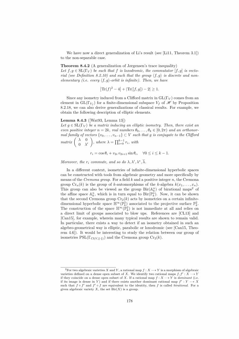
We have now a direct generalization of Li’s result (see [Li11, Theorem 3.1])to the non-separable case.
Theorem 8.4.2 (A generalization of Jørgensen’s trace inequality)Let f, g ∈ SL(ΓV ) be such that f is loxodromic, the commutator [f, g] is vecto-rial (see Definition 8.2.10) and such that the group 〈f, g〉 is discrete and non-elementary (i.e. every 〈f, g〉-orbit is infinite). Then, we have∣∣Tr(f)2 − 4
∣∣+ |Tr([f, g])− 2| ≥ 1.
Since any isometry induced from a Clifford matrix in GL(ΓV ) comes from anelement in GL(ΓVf ) for a finite-dimensional subspace Vf of H by Proposition8.2.18, we can also derive generalizations of classical results. For example, weobtain the following description of elliptic elements.
Lemma 8.4.3 ([Wat93, Lemma 13])Let g ∈ SL(ΓV ) be a matrix inducing an elliptic isometry. Then, there exist aneven positive integer n = 2k, real numbers θ0, . . . , θk ∈ [0, 2π) and an orthonor-mal family of vectors v0, . . . , vn−1 ⊂ V such that g is conjugate to the Clifford
matrix(λ 00 λ′
), where λ =
∏k−1i=0 ri, with
ri = cos θi + v2i v2i+1 sin θi, ∀0 ≤ i ≤ k − 1.
Moreover, the ri commute, and so do λ, λ′, λ∗, λ.
In a different context, isometries of infinite-dimensional hyperbolic spacescan be constructed with tools from algebraic geometry and more specifically bymeans of the Cremona group. For a field k and a positive integer n, the Cremonagroup Crn(k) is the group of k-automorphisms of the k-algebra k(x1, . . . , xn).This group can also be viewed as the group Bir(Ank ) of birational maps2 ofthe affine space Ank , which is in turn equal to Bir(Pnk ). Now, it can be shownthat the second Cremona group Cr2(k) acts by isometries on a certain infinite-dimensional hyperbolic space H∞(P2
k) associated to the projective surface P2k.
The construction of the space H∞(P2k) is not immediate at all and relies on
a direct limit of groups associated to blow ups. References are [CL13] and[Can15], for example, wherein many typical results are shown to remain valid.In particular, there exists a way to detect if an isometry obtained in such analgebro-geometrical way is elliptic, parabolic or loxodromic (see [Can15, Theo-rem 4.6]). It would be interesting to study the relation between our group ofisometries PSL(ΓCl(V,‖·‖)) and the Cremona group Cr2(k).
2For two algebraic varietiesX and Y , a rational map f : X 99K Y is a morphism of algebraicvarieties defined on a dense open subset of X. We identify two rational maps f, f ′ : X 99K Yif they coincide on a dense open subset of X. If a rational map f : X 99K Y is dominant (i.e.if its image is dense in Y ) and if there exists another dominant rational map f ′ : Y 99K Xsuch that f f ′ and f ′ f are equivalent to the identity, then f is called birational. For agiven algebraic variety X, the set Bir(X) is a group.
178

APPENDIXAData
A.1 Kaplinskaya’s prisms in dimension 3
A.1.1 The compact caseWe present in this section the invariants of the compact Coxeter prisms given inFigure A.1 (see [Kap74]). Some details regarding the groups Γ1
m, Γ2m and Γ3
k,m
can be found in Section 4.4.1.
Figure A.1 – Families of 3-dimensional compact prisms
Arithmeticity The following table contains the values for which the group is(quasi-)arithmetic (arithmetic groups are indeed also quasi-arithmetic).
Group Quasi-arithmetic (Quasi-)Arithmetic
Γ1m m = 5, 10 m = 4, 6
Γ2m m = 12 m = 5, 6, 8
Γ33,m m = 12, 18, 24, 30 m = 7, 8, 9, 10, 14
Γ34,m m = 18 m = 7, 8, 10, 12
Continued on next page
179
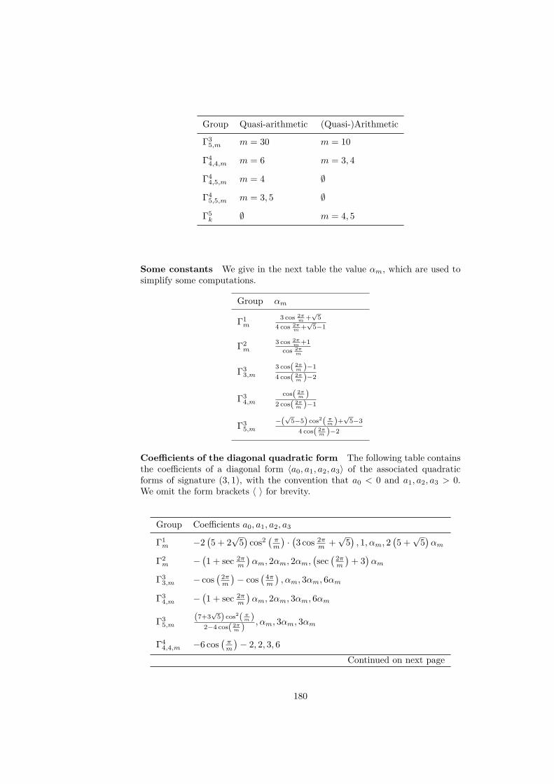
Group Quasi-arithmetic (Quasi-)Arithmetic
Γ35,m m = 30 m = 10
Γ44,4,m m = 6 m = 3, 4
Γ44,5,m m = 4 ∅
Γ45,5,m m = 3, 5 ∅
Γ5k ∅ m = 4, 5
Some constants We give in the next table the value αm, which are used tosimplify some computations.
Group αm
Γ1m
3 cos 2πm +√
54 cos 2π
m +√
5−1
Γ2m
3 cos 2πm +1
cos 2πm
Γ33,m
3 cos( 2πm )−1
4 cos( 2πm )−2
Γ34,m
cos( 2πm )
2 cos( 2πm )−1
Γ35,m
−(√5−5) cos2( πm )+√
5−34 cos( 2π
m )−2
Coefficients of the diagonal quadratic form The following table containsthe coefficients of a diagonal form 〈a0, a1, a2, a3〉 of the associated quadraticforms of signature (3, 1), with the convention that a0 < 0 and a1, a2, a3 > 0.We omit the form brackets 〈 〉 for brevity.
Group Coefficients a0, a1, a2, a3
Γ1m −2
(5 + 2
√5)
cos2 ( πm
)·(3 cos 2π
m +√
5), 1, αm, 2
(5 +√
5)αm
Γ2m −
(1 + sec 2π
m
)αm, 2αm, 2αm,
(sec( 2πm
)+ 3)αm
Γ33,m − cos
( 2πm
)− cos
( 4πm
), αm, 3αm, 6αm
Γ34,m −
(1 + sec 2π
m
)αm, 2αm, 3αm, 6αm
Γ35,m
(7+3√
5) cos2( πm )2−4 cos( 2π
m ) , αm, 3αm, 3αm
Γ44,4,m −6 cos
(πm
)− 2, 2, 3, 6
Continued on next page
180
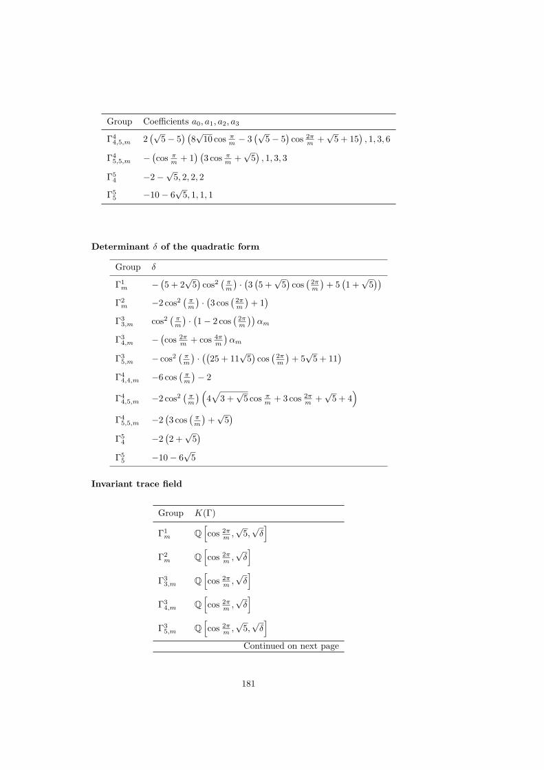
Group Coefficients a0, a1, a2, a3
Γ44,5,m 2
(√5− 5
) (8√
10 cos πm − 3
(√5− 5
)cos 2π
m +√
5 + 15), 1, 3, 6
Γ45,5,m −
(cos π
m + 1) (
3 cos πm +
√5), 1, 3, 3
Γ54 −2−
√5, 2, 2, 2
Γ55 −10− 6
√5, 1, 1, 1
Determinant δ of the quadratic form
Group δ
Γ1m −
(5 + 2
√5)
cos2 ( πm
)·(3(5 +√
5)
cos( 2πm
)+ 5
(1 +√
5))
Γ2m −2 cos2 ( π
m
)·(3 cos
( 2πm
)+ 1)
Γ33,m cos2 ( π
m
)·(1− 2 cos
( 2πm
))αm
Γ34,m −
(cos 2π
m + cos 4πm
)αm
Γ35,m − cos2 ( π
m
)·((
25 + 11√
5)
cos( 2πm
)+ 5√
5 + 11)
Γ44,4,m −6 cos
(πm
)− 2
Γ44,5,m −2 cos2 ( π
m
) (4√
3 +√
5 cos πm + 3 cos 2π
m +√
5 + 4)
Γ45,5,m −2
(3 cos
(πm
)+√
5)
Γ54 −2
(2 +√
5)
Γ55 −10− 6
√5
Invariant trace field
Group K(Γ)
Γ1m Q
[cos 2π
m ,√
5,√δ]
Γ2m Q
[cos 2π
m ,√δ]
Γ33,m Q
[cos 2π
m ,√δ]
Γ34,m Q
[cos 2π
m ,√δ]
Γ35,m Q
[cos 2π
m ,√
5,√δ]
Continued on next page
181
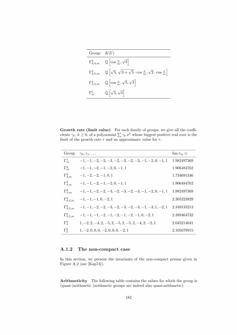
Group K(Γ)
Γ44,4,m Q
[cos π
m ,√δ]
Γ44,5,m Q
[√5,√
3 +√
5 · cos πm ,√
2 · cos πm
]Γ4
5,5,m Q[cos π
m ,√
5,√δ]
Γ5m Q
[√5,√δ]
Growth rate (limit value) For each family of groups, we give all the coeffi-cients γk, k ≥ 0, of a polynomial
∑γk x
k whose biggest positive real root is thelimit of the growth rate τ and an approximate value for τ .
Group γ0, γ1, . . . lim τm '
Γ1m −1,−1,−2,−2,−3,−2,−3,−2,−3,−1,−2, 0,−1, 1 1.982497369
Γ2m −1,−1,−2,−1,−2, 0,−1, 1 1.906484762
Γ33,m −1,−2,−2,−1, 0, 1 1.734691346
Γ34,m −1,−1,−2,−1,−2, 0,−1, 1 1.906484762
Γ35,m −1,−1,−2,−2,−3,−2,−3,−2,−3,−1,−2, 0,−1, 1 1.982497369
Γ44,4,m −1,−1,−1, 0,−2, 1 2.305223929
Γ44,5,m −1,−1,−2,−2,−3,−2,−3,−2,−3,−1,−3, 1,−2, 1 2.349133213
Γ45,5,m −1,−1,−1,−2,−1,−2,−1,−2,−1, 0,−2, 1 2.389464732
Γ54 1,−2, 2,−4, 2,−5, 2,−5, 2,−5, 2,−4, 2,−2, 1 2.045214041
Γ55 1,−2, 0, 0, 0,−2, 0, 0, 0,−2, 1 2.105678915
A.1.2 The non-compact case
In this section, we present the invariants of the non-compact prisms given inFigure A.2 (see [Kap74]).
Arithmeticity The following table contains the values for which the group is(quasi-)arithmetic (arithmetic groups are indeed also quasi-arithmetic).
182

Figure A.2 – Families 3-dimensional non-compact prisms
Group Quasi-arithmetic (Quasi-)Arithmetic
Γ6m m = 6 m = 4
Γ7m ∅ m = 6
Γ8m ∅ ∅
Γ93,m m = 4 ∅
Γ94,m ∅ m = 3
Γ10m ∅ ∅
Γ11k1,k2
∅ k1 = k2 = 4, 6
Determinant δ of the quadratic form
Group δ Group δ
Γ6m -3 Γ9
3,m,Γ94,m -1
Γ7m -1 Γ10
m -3
Γ8m -3 Γ11
k1,k2-3
Invariant trace field
Group K(Γ) Group K(Γ)
Γ6m Q
[i√
3, cos 2πm
]Γ11
3,6 Q[i,√
3]
Γ7m Q
[i, cos 2π
m
]Γ11
4,4 Q[i√
3]
Γ8m Q
[i√
3, cos 2πm
]Γ11
4,5 Q[i√
3,√
2,√
5]
Continued on next page
183

Group K(Γ) Group K(Γ)
Γ93,m Q
[i,√
2 · cos πm
]Γ11
4,6 Q[i√
3,√
6]
Γ94,m Q
[i, cos π
m
]Γ11
5,5 Q[i√
3,√
5]
Γ10m Q
[i√
3, cos πm
]Γ11
5,6 Q[i,√
3,√
5]
Γ113,4 Q
[i√
3,√
2]
Γ116,6 Q
[i√
3]
Γ113,5 Q
[i√
3,√
5]
Growth rate (limit value) For each infinite family of groups, we give allthe coefficients γk, k ≥ 0, of a polynomial
∑γk x
k whose biggest positive realroot is the limit of the growth rate τ and an approximate value for τ .
Group γ0, γ1, . . . lim τm '
Γ6m −1,−2,−1,−1,−1,−1, 1 2.015614858
Γ7m −1,−2,−1,−1, 1 2.065994892
Γ8m −1,−2,−1,−1,−1,−1, 1 2.015614858
Γ93,m −1,−2,−3,−3,−3,−3,−1,−1, 1 2.352041123
Γ94,m −2,−3,−2,−1, 1 2.451109537
Γ10m −2,−1,−1, 0,−2, 1 2.330809311
We now give the growth rate of the remaining 9 prisms Γ11k1,k2.
Group Coefficients γ0, γ1, . . . and growth rate
Γ113,4
−2,−2,−3,−3,−2,−2,−1, 12.459101131
Γ113,5
−2,−2,−5,−6,−7,−9,−8,−9,−8,−8,−6,−5,−3,−1,−1, 12.496678489
Γ113,6
−1,−3,−3,−4,−4,−2,−2,−1, 12.510800457
Γ114,4
−2,−2,−4,−3,−3,−2,−1, 12.548573757
Γ114,5
−2,−2,−6,−6,−9,−9,−10,−9,−10,−8,−8,−5,−4,−1,−1, 12.581500889
Γ114,6
−1,−3,−3,−5,−4,−3,−2,−1, 12.593583812
Continued on next page
184

Group Coefficients γ0, γ1, . . . and growth rate
Γ115,5
−2,−2,−4,−5,−5,−6,−5,−6,−5,−4,−3,−2,−1, 12.612522099
Γ115,6
−1,−3,−3,−5,−6,−6,−6,−6,−6,−6,−4,−3,−2,−1, 12.623816333
Γ116,6
−2,−4,−2,−2,−3,−1, 12.634795548
A.2 Polytopes with n + 3 facets and one non-simple vertex
In [Rob15, v3], Roberts presents the classification of hyperbolic Coxeter poly-topes in Hn with n + 3 facets and one non-simple vertex. We present theinvariants of the commensurability class for the arithmetic groups of his list (38groups among 144). We omit the brackets in the notation of the quadratic form.The invariants were found using a computer and AlVin.
n Group Quadratic form c(V ) δ Invariant
4 8 (a) −6, 1, 3, 6, 6 (−1,−1) −2 Q, 0, 2
4 12(a) −6, 1, 2, 3, 6 (−2,−1) −6 Q, 0, 2
5 13(a) −6, 1, 3, 3, 3, 6 (−3,−1) 3 Q, 3,
5 13(b) −10, 1, 5, 5, 5, 10 (−5,−1) 5 Q, 5,
5 15(a) −5, 1, 5, 10, 15, 30 (−5,−1) 5 Q, 5,
5 15(b) −5, 1, 2, 3, 5, 6 (−2,−1) 1 Q, 0, 2
5 15(d) −3, 1, 2, 3, 3, 6 (−2,−1) 1 Q, 0, 2
5 15(f) −3, 1, 2, 3, 3, 6 (−2,−1) 2 Q, 0, 2
5 16(a) −3, 1, 3, 3, 3, 3 (−3,−1) 3 Q, 3,
5 16(b) −15, 1, 5, 5, 5, 15 (−1,−1) 5 Q, 5,
5 18(a) −2, 1, 1, 2, 2, 2 (−2,−1) 1 Q, 0, 2
5 18(d) −7, 1, 1, 2, 2, 7 (−2,−1) 1 Q, 0, 2
5 18(f) −2, 1, 1, 2, 2, 2 (−2,−1) 1 Q, 0, 2
5 20(a) −1, 1, 1, 1, 2, 2 (−2,−1) 1 Q, 0, 2
5 20(d) −2, 1, 1, 2, 2, 2 (−2,−1) 1 Q, 0, 2
5 20(f) −1, 1, 1, 1, 2, 2 (−2,−1) 1 Q, 0, 2Continued on next page
185
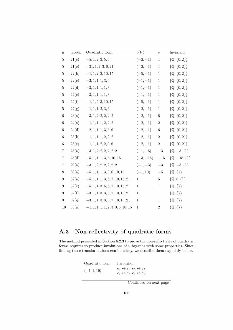
n Group Quadratic form c(V ) δ Invariant
5 21(c) −5, 1, 2, 3, 5, 6 (−2,−1) 1 Q, 0, 2
5 21(e) −21, 1, 2, 3, 6, 21 (−2,−1) 1 Q, 0, 2
5 22(b) −1, 1, 2, 3, 10, 15 (−5,−1) 1 Q, 0, 2
5 22(c) −2, 1, 1, 1, 3, 6 (−1,−1) 1 Q, 0, 2
5 22(d) −3, 1, 1, 1, 1, 3 (−1,−1) 1 Q, 0, 2
5 22(e) −3, 1, 1, 1, 1, 3 (−1,−1) 1 Q, 0, 2
5 22(f) −1, 1, 2, 3, 10, 15 (−5,−1) 1 Q, 0, 2
5 22(g) −1, 1, 1, 2, 3, 6 (−2,−1) 1 Q, 0, 2
6 23(a) −3, 1, 2, 2, 2, 2, 2 (−2,−1) 6 Q, 0, 2
6 24(a) −1, 1, 1, 1, 2, 2, 2 (−2,−1) 2 Q, 0, 2
6 24(d) −2, 1, 1, 1, 3, 6, 6 (−2,−1) 6 Q, 0, 2
6 25(b) −1, 1, 1, 1, 2, 2, 2 (−2,−1) 2 Q, 0, 2
6 25(e) −1, 1, 1, 2, 2, 3, 6 (−2,−1) 2 Q, 0, 2
7 28(a) −3, 1, 2, 2, 2, 2, 2, 2 (−1,−6) −3 Q,−3,
7 28(d) −5, 1, 1, 1, 3, 6, 10, 15 (−3,−15) −15 Q,−15,
7 29(a) −3, 1, 2, 2, 2, 2, 2, 2 (−1,−3) −3 Q,−3,
8 30(a) −5, 1, 1, 1, 3, 3, 6, 10, 15 (−1, 10) −5 Q,
9 32(a) −5, 1, 1, 1, 3, 6, 7, 10, 15, 21 1 5 Q, 5,
9 32(e) −5, 1, 1, 3, 5, 6, 7, 10, 15, 21 1 1 Q,
9 32(f) −3, 1, 1, 3, 3, 6, 7, 10, 15, 21 1 1 Q,
9 32(g) −3, 1, 1, 3, 3, 6, 7, 10, 15, 21 1 1 Q,
10 33(a) −1, 1, 1, 1, 1, 2, 3, 3, 6, 10, 15 1 2 Q,
A.3 Non-reflectivity of quadratic formsThe method presented in Section 6.2.3 to prove the non-reflectivity of quadraticforms requires to produce involutions of subgraphs with some properties. Sincefinding these transformations can be tricky, we describe them explicitly below.
Quadratic form Involution
〈−1, 1, 19〉 e4 ↔ e8, e6 ↔ e7e1 ↔ e6, e5 ↔ e8
Continued on next page
186
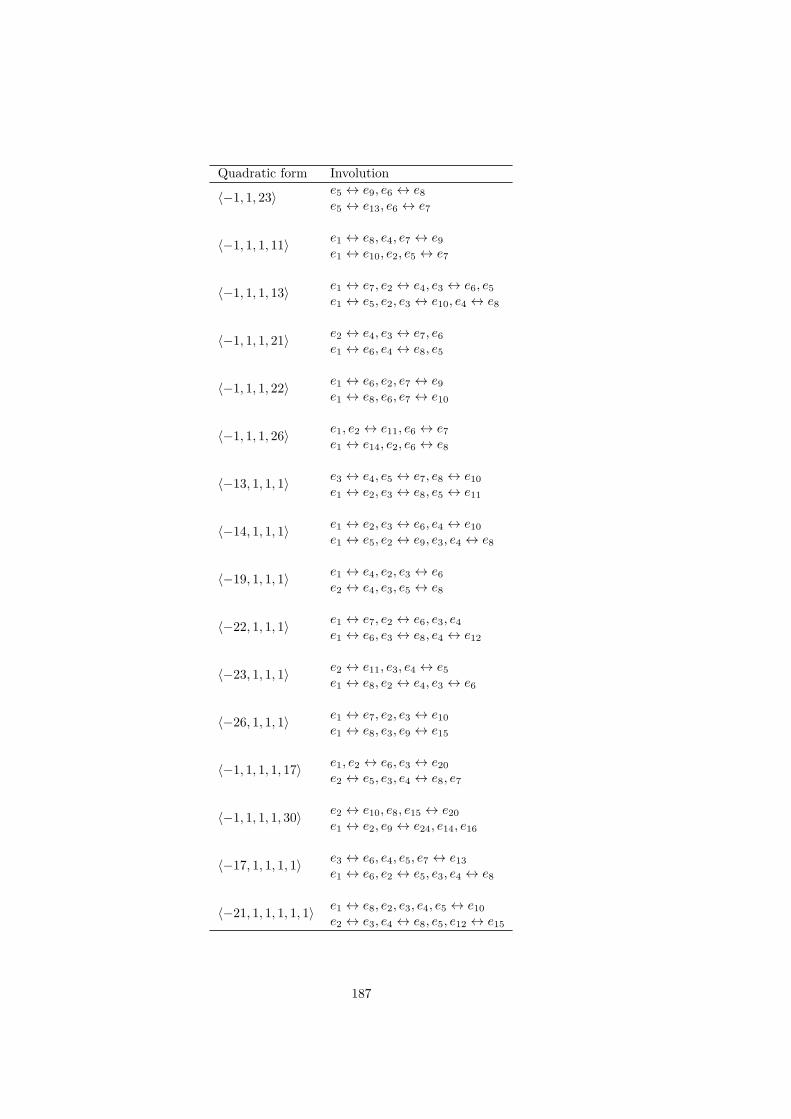
Quadratic form Involution
〈−1, 1, 23〉 e5 ↔ e9, e6 ↔ e8e5 ↔ e13, e6 ↔ e7
〈−1, 1, 1, 11〉 e1 ↔ e8, e4, e7 ↔ e9e1 ↔ e10, e2, e5 ↔ e7
〈−1, 1, 1, 13〉 e1 ↔ e7, e2 ↔ e4, e3 ↔ e6, e5e1 ↔ e5, e2, e3 ↔ e10, e4 ↔ e8
〈−1, 1, 1, 21〉 e2 ↔ e4, e3 ↔ e7, e6e1 ↔ e6, e4 ↔ e8, e5
〈−1, 1, 1, 22〉 e1 ↔ e6, e2, e7 ↔ e9e1 ↔ e8, e6, e7 ↔ e10
〈−1, 1, 1, 26〉 e1, e2 ↔ e11, e6 ↔ e7e1 ↔ e14, e2, e6 ↔ e8
〈−13, 1, 1, 1〉 e3 ↔ e4, e5 ↔ e7, e8 ↔ e10e1 ↔ e2, e3 ↔ e8, e5 ↔ e11
〈−14, 1, 1, 1〉 e1 ↔ e2, e3 ↔ e6, e4 ↔ e10e1 ↔ e5, e2 ↔ e9, e3, e4 ↔ e8
〈−19, 1, 1, 1〉 e1 ↔ e4, e2, e3 ↔ e6e2 ↔ e4, e3, e5 ↔ e8
〈−22, 1, 1, 1〉 e1 ↔ e7, e2 ↔ e6, e3, e4e1 ↔ e6, e3 ↔ e8, e4 ↔ e12
〈−23, 1, 1, 1〉 e2 ↔ e11, e3, e4 ↔ e5e1 ↔ e8, e2 ↔ e4, e3 ↔ e6
〈−26, 1, 1, 1〉 e1 ↔ e7, e2, e3 ↔ e10e1 ↔ e8, e3, e9 ↔ e15
〈−1, 1, 1, 1, 17〉 e1, e2 ↔ e6, e3 ↔ e20e2 ↔ e5, e3, e4 ↔ e8, e7
〈−1, 1, 1, 1, 30〉 e2 ↔ e10, e8, e15 ↔ e20e1 ↔ e2, e9 ↔ e24, e14, e16
〈−17, 1, 1, 1, 1〉 e3 ↔ e6, e4, e5, e7 ↔ e13e1 ↔ e6, e2 ↔ e5, e3, e4 ↔ e8
〈−21, 1, 1, 1, 1, 1〉 e1 ↔ e8, e2, e3, e4, e5 ↔ e10e2 ↔ e3, e4 ↔ e8, e5, e12 ↔ e15
187
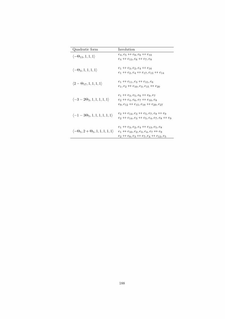
Quadratic form Involution
〈−Θ13, 1, 1, 1〉e4, e5 ↔ e8, e6 ↔ e10e4 ↔ e13, e6 ↔ e7, e8
〈−Θ3, 1, 1, 1, 1〉e1 ↔ e3, e2, e4 ↔ e16e1 ↔ e2, e4 ↔ e17, e13 ↔ e14
〈2−Θ17, 1, 1, 1, 1〉e1 ↔ e11, e3 ↔ e15, e6e1, e2 ↔ e10, e3, e15 ↔ e20
〈−3− 2Θ3, 1, 1, 1, 1, 1〉e1 ↔ e3, e5, e6 ↔ e9, e7e2 ↔ e4, e6, e7 ↔ e10, e8e9, e12 ↔ e15, e18 ↔ e29, e27
〈−1− 3Θ5, 1, 1, 1, 1, 1, 1〉e2 ↔ e14, e3 ↔ e5, e7, e8 ↔ e9e2 ↔ e14, e3 ↔ e5, e4, e7, e8 ↔ e9
〈−Θ5, 2 + Θ5, 1, 1, 1, 1, 1〉e1 ↔ e3, e2, e4 ↔ e13, e5, e8e1 ↔ e10, e2, e3, e4, e7 ↔ e9e2 ↔ e8, e3 ↔ e7, e4 ↔ e13, e5
188
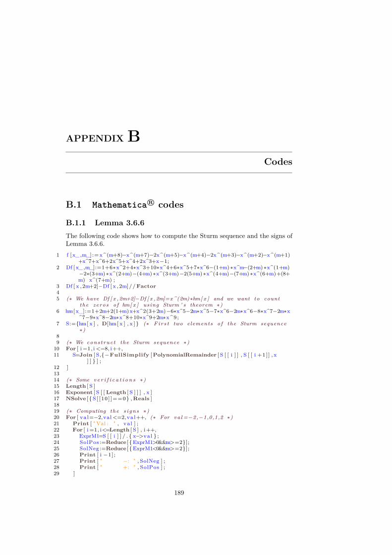
APPENDIXBCodes
B.1 Mathematica R© codes
B.1.1 Lemma 3.6.6The following code shows how to compute the Sturm sequence and the signs ofLemma 3.6.6.
1 f [ x_,m_] :=x^(m+8)−x^(m+7)−2x^(m+5)−x^(m+4)−2x^(m+3)−x^(m+2)−x^(m+1)+x^7+x^6+2x^5+x^4+2x^3+x−1;
2 Df [ x_,m_]:=1+6∗x^2+4∗x^3+10∗x^4+6∗x^5+7∗x^6−(1+m) ∗x^m−(2+m) ∗x^(1+m)−2∗(3+m) ∗x^(2+m)−(4+m) ∗x^(3+m)−2(5+m) ∗x^(4+m)−(7+m) ∗x^(6+m)+(8+m) x^(7+m) ;
3 Df [ x , 2m+2]−Df [ x , 2m]//Factor45 (∗ We have Df [ x ,2m+2]−Df [ x ,2m]=x ^(2m)∗hm[ x ] and we want to count
the zeros o f hm[ x ] us ing Sturm ’ s theorem ∗)6 hm[x_]:=1+2m+2(1+m)x+x^2(3+2m)−6∗x^5−2m∗x^5−7∗x^6−2m∗x^6−8∗x^7−2m∗x
^7−9∗x^8−2m∗x^8+10∗x^9+2m∗x ^9 ;7 S:=hm[ x ] , D[hm[ x ] , x ] (∗ F i r s t two elements o f the Sturm sequence
∗)89 (∗ We c o n s t r u c t the Sturm sequence ∗)
10 For [ i =1, i <=8, i++,11 S=Join [ S,−FullSimplify [PolynomialRemainder [ S [ [ i ] ] , S [ [ i +1 ] ] , x
] ] ] ;12 ]1314 (∗ Some v e r i f i c a t i o n s ∗)15 Length [ S ]16 Exponent [ S [ [ Length [ S ] ] ] , x ]17 NSolve [ S [ [ 10 ] ]==0 ,Reals ]1819 (∗ Computing the s i g n s ∗)20 For [ va l=−2,val <=2,va l++, (∗ For v a l =−2,−1,0,1,2 ∗)21 Print [ " Val : " , va l ] ;22 For [ i =1, i<=Length [ S ] , i++,23 ExprM1=S [ [ i ] ] / . x−>val ;24 SolPos :=Reduce [ ExprM1>0&&m>=2];25 SolNeg :=Reduce [ ExprM1<0&&m>=2];26 Print [ i −1] ;27 Print [ " −: " , SolNeg ] ;28 Print [ " +: " , SolPos ] ;29 ]
189
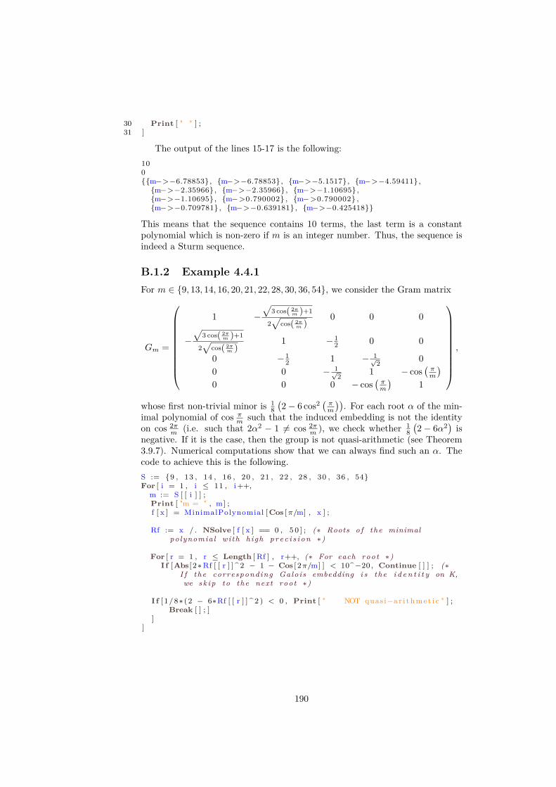
30 Print [ " " ] ;31 ]
The output of the lines 15-17 is the following:100m−>−6.78853, m−>−6.78853, m−>−5.1517, m−>−4.59411,
m−>−2.35966, m−>−2.35966, m−>−1.10695,m−>−1.10695, m−>0.790002 , m−>0.790002 ,m−>−0.709781, m−>−0.639181, m−>−0.425418
This means that the sequence contains 10 terms, the last term is a constantpolynomial which is non-zero if m is an integer number. Thus, the sequence isindeed a Sturm sequence.
B.1.2 Example 4.4.1For m ∈ 9, 13, 14, 16, 20, 21, 22, 28, 30, 36, 54, we consider the Gram matrix
Gm =
1 −√
3 cos( 2πm )+1
2√
cos( 2πm )
0 0 0
−√
3 cos( 2πm )+1
2√
cos( 2πm )
1 − 12 0 0
0 − 12 1 − 1√
2 00 0 − 1√
2 1 − cos(πm
)0 0 0 − cos
(πm
)1
,
whose first non-trivial minor is 18(2− 6 cos2 ( π
m
)). For each root α of the min-
imal polynomial of cos πm such that the induced embedding is not the identity
on cos 2πm (i.e. such that 2α2 − 1 6= cos 2π
m ), we check whether 18(2− 6α2) is
negative. If it is the case, then the group is not quasi-arithmetic (see Theorem3.9.7). Numerical computations show that we can always find such an α. Thecode to achieve this is the following.S := 9 , 13 , 14 , 16 , 20 , 21 , 22 , 28 , 30 , 36 , 54For [ i = 1 , i ≤ 11 , i++,
m := S [ [ i ] ] ;Print [ "m = " , m] ;f [ x ] = MinimalPolynomial [Cos [π/m] , x ] ;
Rf := x / . NSolve [ f [ x ] == 0 , 5 0 ] ; (∗ Roots o f the minimalpolynomial with high p r e c i s i o n ∗)
For [ r = 1 , r ≤ Length [ Rf ] , r++, (∗ For each root ∗)I f [Abs [ 2∗Rf [ [ r ] ] ^ 2 − 1 − Cos [ 2π/m] ] < 10^−20 , Continue [ ] ] ; (∗
I f the corresponding Galois embedding i s the i d e n t i t y on K,we s k i p to the next root ∗)
I f [ 1/8∗ (2 − 6∗Rf [ [ r ] ] ^ 2 ) < 0 , Print [ " NOT quasi−a r i thmet i c " ] ;Break [ ] ; ]
]]
190

Bibliography
[AF06] S. Agarwal and G. S. Frandsen. “A new GCD algorithm for qua-dratic number rings with unique factorization”. In: LATIN 2006:Theoretical Informatics. Springer, 2006, pp. 30–42.
[Ahl85] L. V. Ahlfors. “Möbius transformations and Clifford numbers”. In:Differential geometry and complex analysis. Springer, 1985, pp. 65–73.
[All06] D. Allcock. “Infinitely many hyperbolic Coxeter groups through di-mension 19”. In: Geometry & Topology 10.2 (2006), pp. 737–758.
[Alo91] J. M. Alonso. “Growth functions of amalgams”. In: Arboreal GroupTheory. Springer, 1991, pp. 1–34.
[AMR09] O. Antolin-Camarena, G. R. Maloney, and R. K. W. Roeder. “Com-puting Arithmetic Invariants for Hyperbolic Reflection Groups”. In:doi:10.1201/b10617-22. A K Peters/CRC Press, Nov. 2009, pp. 597–631. isbn: 978-1-56881-450-6.
[BIM05] M. Burger, A. Iozzi, and N. Monod. “Equivariant embeddings oftrees into hyperbolic spaces”. In: International Mathematics Re-search Notices 2005.22 (2005), pp. 1331–1369. url: https://arxiv.org/abs/math/0404530.
[Bor62] A. Borel. “Arithmetic subgroups of algebraic groups”. In: Annals ofmathematics (1962), pp. 485–535.
[Bor87] R. Borcherds. “Automorphism groups of Lorentzian lattices”. In:Journal of Algebra 111.1 (1987), pp. 133–153.
[Bou68a] N. Bourbaki. Elements de mathematique, fasc. 34: groupes et al-gèbres de Lie, chap. 4, 5 et 6. Hermann, 1968.
[Bou68b] N. Bourbaki. Groupes et algèbres de Lie IV-VI. Hermann, Paris,1968.
[Bug84] V. Bugaenko. “Groups of automorphisms of unimodular hyperbolicquadratic forms over the ring Z[(1 +
√5)/2]”. In: Moscow Univ.
Math. Bull 39 (1984), pp. 6–14.[Bug90] V. Bugaenko. “On reflective unimodular hyperbolic quadratic
forms”. In: Selecta Math. Soviet 9.3 (1990), pp. 263–271.[Bug92] V. Bugaenko. “Arithmetic crystallographic groups generated by re-
flections, and reflective hyperbolic lattices”. In: Lie groups, their dis-crete subgroups, and invariant theory 8 (1992), pp. 33–55.
191

[Can15] S. Cantat. “The Cremona group”. In: Proceedings of 2015 SummerInstitute on Algebraic Geometry. Ed. by AMS Proceedings of Sym-posia in Pure Mathematics. 2015. url: https : / / perso . univ -rennes1.fr/serge.cantat/Articles/Survey-Cremona-SLC.pdf.
[Cas78] J. W. S. Cassels. Rational quadratic forms. Vol. 13. London Mathe-matical Society Monographs. Academic Press, Inc. [Harcourt BraceJovanovich, Publishers], London-New York, 1978, pp. xvi+413. isbn:0-12-163260-1.
[CF67] J. W. S. Cassels and A. Fröhlich. Algebraic number theory. AcademicPress, Inc. [Harcourt Brace Jovanovich, Publishers], London-NewYork, 1967.
[CL13] Serge Cantat and Stéphane Lamy. “Normal subgroups in the Cre-mona group (long version)”. In: Acta Math. 210.1 (2013). With anappendix by Yves de Cornulier, pp. 31–94. issn: 0001-5962.
[Cla94] D. A. Clark. “A quadratic field which is Euclidean but not norm-Euclidean”. In: manuscripta mathematica 83.1 (1994), pp. 327–330.
[CM72] H. S. M. Coxeter and W. O. J. Moser. Generators and relations fordiscrete groups. Third. Springer, Berlin, 1972.
[Coh93] H. Cohen. A Course in Computational Number Theory. Third. Grad-uate Texts in Mathematics. Springer, 1993. isbn: 3-540-55640-0.
[Con85] J. B. Conway. A course in functional analysis. Vol. 96. SpringerScience & Business Media, 1985.
[Cox35] H. S. M. Coxeter. “The complete enumeration of finite groups of theform R2
i = (RiRj)kij = 1”. In: Journal of the London MathematicalSociety 1 (1935).
[CW92] J. W. Cannon and P. Wagreich. “Growth functions of surfacegroups”. In: Mathematische Annalen 293.1 (1992), pp. 239–257.
[Das12] T. Das. “Kleinian groups in Hilbert spaces”. PhD thesis. 2012.[EIR11] M. Elia, J. C. Interlando, and R. Rosenbaum. “On the Structure of
Residue Rings of Prime Ideals in Algebraic Number Fields–Part II:Ramified Primes”. In: International Mathematical Forum. Vol. 6. 12.2011, pp. 565–589.
[ERT15] V. Emery, J. Ratcliffe, and S. Tschantz. “Salem numbers andarithmetic hyperbolic groups”. In: arXiv preprint arXiv:1506.03727(2015).
[Ess96] F. Esselmann. “The classification of compact hyperbolic Coxeter d-polytopes with d+2 facets”. In: Commentarii Mathematici Helvetici71.1 (1996), pp. 229–242.
[Flo92] W. J. Floyd. “Growth of planar Coxeter groups, P.V. numbers, andSalem numbers”. In: Mathematische Annalen 293.1 (1992), pp. 475–483. issn: 0025-5831.
[Fru91] Monica Frunza. “Möbius transformations in infinite dimension”. In:Rev. Roumaine Math. Pures. Appl. 36 (1991), pp. 369–376.
192
[FTZ07] A. Felikson, P. Tumarkin, and T. Zehrt. “On hyperbolic Coxeter n-polytopes with n+ 2 facets”. In: Advances in Geometry 7.2 (2007),pp. 177–189.
[Gal05] S. R. Gal. “On normal subgroups of Coxeter groups generatedby standard parabolic subgroups”. In: Geometriae Dedicata 115.1(2005), pp. 65–78.
[GJK16] R. Guglielmetti, M. Jacquemet, and R. Kellerhals. “On commen-surable hyperbolic Coxeter groups”. In: Geometriae Dedicata 183.1(2016), pp. 143–167.
[GJKar] R. Guglielmetti, M. Jacquemet, and R. Kellerhals. “Commensura-bility of hyperbolic Coxeter groups: theory and computation”. In:Discrete Groups and Hyperbolic Geometry. Ed. by M. Fujii. RIMSKôkyûroku Bessatsu. to appear. 50 pp.
[GP87] M. Gromov and I. Piatetski-Shapiro. “Non-arithmetic groups in Lo-bachevsky spaces”. In: Publications Mathématiques de l’IHÉS 66(1987), pp. 93–103.
[Gri07] P. A. Grillet. Abstract algebra. Vol. 242. Springer Science & BusinessMedia, 2007.
[Gro08] J. Grosek. “Fundamental reflection domains for hyperbolic tesse-lations”. In: Rose-Hulman Undergraduate Mathematics Journal 9.1(2008).
[GS06] P. Gille and T. Szamuely. Central simple algebras and Galois coho-mology. Vol. 101. Cambridge University Press, 2006.
[Gug15] R. Guglielmetti. “CoxIter - Computing invariants of hyperbolic Cox-eter groups”. In: LMS Journal of Computation and Mathematics 18.1(Dec. 2015), pp. 754–773. doi: 10.1112/S146115701500027. url:https://dx.doi.org/10.1112/S1461157015000273.
[Hen74] P. Henrici. Applied and computational complex analysis. English.Vol. 1. John Wiley & Sons Ltd, 1974, pp. xv + 682.
[Hil07] T. Hild. “Cusped hyperbolic orbifolds of minimal volume in dimen-sions less than 11”. PhD thesis. University of Fribourg, 2007.
[HS04] N. Howgrave-Graham and M. Szydlo. “A Method to Solve Cy-clotomic Norm Equations f ? f”. In: Algorithmic Number Theory.Springer, 2004, pp. 272–279.
[Huf76] M. Huff. “Conformal maps on Hilbert space”. In: Bulletin of theAmerican Mathematical Society 82.1 (1976), pp. 147–149.
[HW08] G. H. Hardy and E. Wright. An Introduction to the Theory of Num-bers. 6th ed. Oxford University Press, 2008.
[Im 85] H.-C. Im Hof. “A class of hyperbolic Coxeter groups”. In: Expo. Math3 (1985), pp. 179–186.
[Im 90] H.-C. Im Hof. “Napier cycles and hyperbolic Coxeter groups”. In:Bull. Soc. Math. Belg. Sér. A 42.3 (1990), pp. 523–545.
[Joh+02] N. W. Johnson, R. Kellerhals, J. Ratcliffe, and S. Tschantz. “Com-mensurability classes of hyperbolic Coxeter groups”. In: Linear al-gebra and its applications 345.1 (2002), pp. 119–147.
193
[Joh+99] N. W. Johnson, R. Kellerhals, J. Ratcliffe, and S. Tschantz. “Thesize of a hyperbolic Coxeter simplex”. In: Transformation Groups4.4 (1999), pp. 329–353.
[Kap74] I. Kaplinskaya. “Discrete groups generated by reflections in the facesof symplicial prisms in Lobachevskian spaces”. In: MathematicalNotes of the Academy of Sciences of the USSR 15.1 (1974), pp. 88–91.
[Kel13] R. Kellerhals. “Cofinite hyperbolic Coxeter groups, minimal growthrate and Pisot numbers”. In: Algebraic & Geometric Topology 13.2(2013), pp. 1001–1025.
[Kel14] R. Kellerhals. “Hyperbolic orbifolds of minimal volume”. In: Com-putational Methods and Function Theory 14.2-3 (2014), pp. 465–481.
[Kel91] R. Kellerhals. “The dilogarithm and volumes of hyperbolic poly-topes”. In: AMS Mathematical Surveys and Monographs 37 (1991),pp. 301–336.
[Kli95] W. P. A. Klingenberg. Riemannian geometry. Vol. 1. Walter deGruyter, 1995.
[Kol12] A. Kolpakov. “Deformation of finite-volume hyperbolic Coxeter poly-hedra, limiting growth rates and Pisot numbers”. In: European Jour-nal of Combinatorics 33.8 (2012), pp. 1709–1724.
[KP11] R. Kellerhals and G. Perren. “On the growth of cocompact hyper-bolic Coxeter groups”. In: European Journal of Combinatorics 32.8(2011), pp. 1299–1316.
[KV78] I. M. Kaplinskaja and È. Vinberg. “On the groups O18,1(Z) andO19,1(Z)”. In: Soviet Mathematics 19.1 (1978), pp. 194–197.
[Lam05] T.-Y. Lam. Introduction to quadratic forms over fields. GraduateStudies in Mathematics. Vol. 67. American Mathematical Soc., 2005.
[Lax02] P. D. Lax. Functional Analysis. New-York: Wiley-Interscience, 2002.[Len75] H. W. Lenstra Jr. “Euclid’s algorithm in cyclotomic fields”. In: J.
London Math. Soc 10 (1975), pp. 457–465.[Li11] L. Li. “A generalization of Jørgensen’s inequality to infinite dimen-
sion”. In: New York Journal of Mathematics 17 (2011), pp. 41–49.url: http://nyjm.albany.edu/j/2011/17-3p.pdf.
[Mac11] C. Maclachlan. “Commensurability classes of discrete arithmetic hy-perbolic groups”. In: Groups, Geometry, and Dynamics 5.4 (2011),pp. 767–785.
[Mar12] A. Mark. Reflection groups of the quadratic form −px20 +x2
1 +...+x2n.
2012. arXiv: 1207.4822 [math]. url: https://arxiv.org/abs/1207.4822.
[Mcl11] J. Mcleod. “Hyperbolic reflection groups associated to the quadraticforms −3x2
0 + x21 + · · ·+ x2
n”. In: Geometriae Dedicata 152.1 (2011),pp. 1–16.
[Mcl13] J. Mcleod. “Arithmetic hyperbolic reflection groups”. PhD thesis.Durham University, 2013.
194
[Mer82] A. Merkurjev. “On the norm residue symbol of degree 2”. In: SovietMath. Dokl. 24 (1982), pp. 1546–1551.
[MR03] C. Maclachlan and A. W. Reid. The arithmetic of hyperbolic 3-manifolds. Vol. 219. Springer Science & Business Media, 2003.
[MR98] C. Maclachlan and A. W. Reid. “Invariant trace-fields and quater-nion algebras of polyhedral groups”. In: Journal of the London Math-ematical Society 58.03 (1998), pp. 709–722.
[Nag52] J. Nagura. “On the interval containing at least one prime number”.In: Proceedings of the Japan Academy 28.4 (1952), pp. 177–181.
[Neu99] J. Neukirch. “Algebraic number theory”. In: (1999).[NZM08] I. Niven, H. Zuckerman, and H. Montgomery. An introduction to the
theory of numbers. Fifth. John Wiley & Sons, 2008. isbn: 978-0-471-62546-9.
[Par93] W. Parry. “Growth series of Coxeter groups and Salem numbers”.In: Journal of Algebra 154.2 (1993), pp. 406–415.
[Per09] G. Perren. “Growth of cocompact hyperbolic Coxeter groups andtheir rate”. PhD thesis. University of Fribourg, 2009.
[Poi93] H. Poincaré. “Sur la généralisation d’un théoreme d’Euler relatifaux polyedres”. In: Comptes Rendus de Séances de l’Academie desSciences 117 (1893), p. 144.
[Pro87] M. N. Prokhorov. “The absence of discrete reflection groups withnoncompact fundamental polyhedron of finite volume in Lobachev-sky space of large dimension”. In: Izvestiya: Mathematics 28.2(1987), pp. 401–411.
[Rat06] J. Ratcliffe. Foundations of hyperbolic manifolds. Vol. 149. SpringerScience & Business Media, 2006.
[Rob04] J. Robertson. Solving the generalized Pell equation x2 −Dy2 = N .2004. url: http://www.jpr2718.org/pell.pdf.
[Rob15] M. Roberts. A Classification of Non-Compact Coxeter Polytopes withn+3 Facets and One Non-Simple Vertex. 2015. arXiv: 1511.08451v3[math].
[RS02] Q. I. Rahman and G. Schmeisser. Analytic theory of polynomials.Oxford University Press, 2002.
[RT13] J. Ratcliffe and S. Tschantz. “On volumes of hyperbolic Coxeterpolytopes and quadratic forms”. In: Geometriae Dedicata 163.1(2013), pp. 285–299.
[RT97] J. Ratcliffe and S. Tschantz. “Volumes of integral congruence hyper-bolic manifolds”. In: Journal für die reine und angewandte Mathe-matik 488 (Jan. 1997).
[Sal63] R. Salem. Algebraic numbers and Fourier analysis. Wadsworth Com-pany, 1963.
[Sch89] R. Scharlau. “On the classification of arithmetic reflection groups onhyperbolic 3-space”. In: preprint, Bielefeld (1989).
195

[Ser96] J.-P. Serre. A course in arithmetic. Vol. 7. Springer-Verlag, NewYork, 1996.
[Ste68] R. Steinberg. Endomorphisms of linear algebraic groups. Memoirsof the American Mathematical Society 80. American MathematicalSociety, 1968.
[Tak75] K. Takeuchi. “A characterization of arithmetic Fuchsian groups”. In:Journal of the Mathematical Society of Japan 27.4 (1975), pp. 600–612.
[Tak77a] K. Takeuchi. “Arithmetic triangle groups”. In: Journal of the Math-ematical Society of Japan 29.1 (1977), pp. 91–106.
[Tak77b] K. Takeuchi. “Commensurability classes of arithmetic trianglegroups”. In: Journal of the Faculty of Science, the University ofTokyo 24 (1977), pp. 201–212.
[Ter15] T. Terragni. Data about hyperbolic Coxeter systems. 2015. arXiv:1503.08764 [math]. url: https://arxiv.org/abs/1503.08764?context=math.GR.
[Tum04] P. Tumarkin. “Hyperbolic Coxeter n-polytopes with n + 2 facets”.In: Mathematical Notes 75.5-6 (2004), pp. 848–854.
[Vig80] M.-F. Vigneras. Arithmétique des algèbres de quaternions. Vol. 800.Springer-Verlag, 1980.
[Vin15] È. Vinberg. “Non-arithmetic hyperbolic reflection groups in higherdimensions”. In:Moscow Mathematical Journal 15.3 (2015), pp. 593–602.
[Vin67] È. Vinberg. “Discrete groups generated by reflections in Lobacevskiispaces”. In: Sbornik: Mathematics 1.3 (1967), pp. 429–444.
[Vin72] È. Vinberg. “On groups of unit elements of certain quadratic forms”.In: Sbornik: Mathematics 16.1 (1972), pp. 17–35.
[Vin81] È. Vinberg. “Absence of crystallographic groups of reflections inLobachevskii spaces of large dimension”. In: Functional Analysis andIts Applications 15.2 (1981), pp. 128–130.
[Vin85] È. Vinberg. “Hyperbolic reflection groups”. In: Russian Mathemati-cal Surveys 40.1 (1985), pp. 31–75.
[Vin88] È. Vinberg. Geometry. II, Encyclopaedia of Mathematical Sciences,29. 1988.
[Was82] L. Washington. Introduction to cyclotomic fields. Springer, 1982.[Wat93] P. Waterman. “Möbius transformations in several dimensions”. In:
Advances in Mathematics 101.1 (1993), pp. 87–113.[Wei80] J. Weidmann. Linear operators in Hilbert spaces. Springer New York,
1980.
196

[Wik05] D. Wikström. “On the l-ary GCD-algorithm in rings of integers”. In:Automata, Languages and Programming: 32nd International Collo-quium, ICALP 2005, Lisbon, Portugal, July 11-15, 2005. Proceed-ings. Ed. by L. Caires, G. F. Italiano, L. Monteiro, C. Palamidessi,and M. Yung. Berlin, Heidelberg: Springer Berlin Heidelberg, 2005,pp. 1189–1201. doi: 10.1007/11523468_96. url: http://dx.doi.org/10.1007/11523468_96.
[Wik15] D. Wikström. private correspondence. 2015.[Yuk16a] T. Yukita. “On the growth rates of cofinite 3-dimensional Coxeter
groups some of whose dihedral angles are πm for m ≥ 7”. In: arXiv
preprint arXiv:1603.04987 (2016). arXiv: 1603.04987 [math]. url:https://arxiv.org/abs/1603.04987?context=math.GR.
[Yuk16b] T. Yukita. “On the growth rates of cofinite 3-dimensional Coxetergroups whose dihedral angles are of the form π
m for m = 2, 3, 4, 5, 6”.In: arXiv preprint arXiv:1603.04592 (2016). arXiv: 1603 . 04592[math]. url: https://arxiv.org/abs/1603.04592?context=math.GR.
[Zeh09] T. Zehrt. “The covolume of discrete subgroups of IsomH2m”. In:Discrete Mathematics 309.8 (2009), pp. 2284–2291.
197
Index
Absolute value, 14Admissible
quadratic form, 48vertex, 151
Amalgamated product, 93Arithmetic group, 48Arithmeticity criterion, 50Atlas, 27
equivalence of, 27
Boundaryof Hn, 30
Brauer group, 17
Cellof a group, 37
Centerof the Clifford algebra, 166
Classificationof quadratic forms, 140
Cliffordalgebra, 164group, 168matrix, 170, 172
Cocompact, 40Cofinite, 40Commensurable
groups, 57topological spaces, 57
Completely ramified prime, 11Conformal map, 27Conjecture
about the evolution of the growthrate, 162
of Kellerhals and Perren, 97Covolume, 40Coxeter
Geometric Coxeter group, 38graph, 36, 39group, 36
CoxIterGAP, 97CoxIterWeb, 80Criterion
for arithmeticity, 50, 87for cocompactness, 48for cofiniteness, 48for reflectivity, 117, 118
Cyclein a graph, 52in a matrix, 50
Decompositionof a prime ideal, 10
Descartes’ rule of signs, 22Determinant
of a Clifford matrix, 170Diffeomorphism, 26Differentiable
atlas, 27manifold, 27map, 26structure, 27
Dimensionof a Hilbert space, 24
Dirichlet’s unit theorem, 10
Elliptic transformation, 35Euclidean
function, 12ring, 12
Euler characteristic, 46
f -vector, 47Field extension, 7
normal, 9simple, 7
Finite place, 14Fundamental unit, 10
Galois
198
extension, 9group, 9
GAP, 97GCD computation, 12Generalized sphere, 25Geometric Coxeter group, 38Gram matrix
of a geometric Coxeter group, 38of a polyhedron, 38
Growthrate, 41, 83rate, example, 43series, 40, 83
Hasse invariant, 64Hilbert
dimension, 24manifold, 26orthonormal basis, 23
Hilbert spacedefinition, 23dimension, 24separable, 24tensor product, 25
Hyperbolic spacehyperboloid model, 30, 32Poincaré ball model, 32upper half-space model, 31vector space model, 30, 32
Hyperboloid model, 30, 32Hyperplane
of Hn, 30
Inert prime, 11Infinite place, 14Invariant
of Hasse, 64of Witt, 63quaternion algebra, 59, 70trace field, 59, 69
IrreducibleCoxeter group, 36
Loxodromic transformation, 35, 179
Möbius transformation, 28
Norm, 13equation, 115
Normal field extension, 9Number field, 9
place, 14
Orthonormal basis, 23
Parabolicsubgroup, 151transformation, 35, 179
Parallelhyperplanes, 31
Perron numberconjecture, 97definition, 14
Pisot number, 15Place of a number field, 14Poincaré
ball model, 32extension, 33series, 40
Polyhedron, 37Prime
decomposition, 10inert, 11ramified, 11unramified, 11
Quadratic formadmissible, 48reflective, 50, 110, 116
Quaternion algebra, 18
Ramificationindex, 10of a quaternion algebra, 19
Rankof a Coxeter graph graph, 39of a geometric Coxeter group, 39
Reflective quadratic form, 50, 110, 116Riemannian
metric, 27Riemannian manifold, 27Ring of integers, 9Root
of a quadratic lattice, 112
Salem numberdefinition, 15
Scharlau’s quadratic forms, 138Separable
element, 8extension, 8Hilbert space, 24
199
Sign changes, 22Similarity, 26Simple field extension, 7Simplest type
arithmetic group of the, 49Splitting field, 8Standard parabolic subgroup, 151Sturm’
sequence, 22theorem, 23
Subgroup relations, 58Symbol, 41
Tensor product of Hilbert spaces, 25Tits form, 38Topological manifold, 26Trace
in a number field, 13of a Clifford matrix, 172
Ultraparallelhyperplanes, 31
Underlying quadratic form, 61Unramified prime, 11
Valuation, 14Vector, 168Vector space, 30Vectorial Clifford matrix, 172Vertex
at infinity, 39Vinberg algorithm, 109
Witt invariant, 63
200
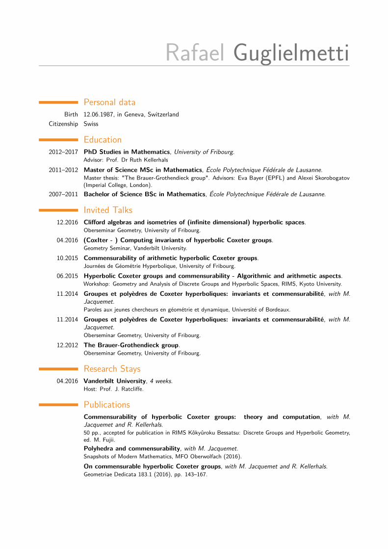
Rafael GuglielmettiPersonal data
Birth 12.06.1987, in Geneva, SwitzerlandCitizenship Swiss
Education2012–2017 PhD Studies in Mathematics, University of Fribourg.
Advisor: Prof. Dr Ruth Kellerhals2011–2012 Master of Science MSc in Mathematics, École Polytechnique Fédérale de Lausanne.
Master thesis: "The Brauer-Grothendieck group". Advisors: Eva Bayer (EPFL) and Alexei Skorobogatov(Imperial College, London).
2007–2011 Bachelor of Science BSc in Mathematics, École Polytechnique Fédérale de Lausanne.
Invited Talks12.2016 Clifford algebras and isometries of (infinite dimensional) hyperbolic spaces.
Oberseminar Geometry, University of Fribourg.04.2016 (CoxIter - ) Computing invariants of hyperbolic Coxeter groups.
Geometry Seminar, Vanderbilt University.10.2015 Commensurability of arithmetic hyperbolic Coxeter groups.
Journées de Géométrie Hyperbolique, University of Fribourg.06.2015 Hyperbolic Coxeter groups and commensurability - Algorithmic and arithmetic aspects.
Workshop: Geometry and Analysis of Discrete Groups and Hyperbolic Spaces, RIMS, Kyoto University.11.2014 Groupes et polyèdres de Coxeter hyperboliques: invariants et commensurabilité, with M.
Jacquemet.Paroles aux jeunes chercheurs en géométrie et dynamique, Université of Bordeaux.
11.2014 Groupes et polyèdres de Coxeter hyperboliques: invariants et commensurabilité, with M.Jacquemet.Oberseminar Geometry, University of Fribourg.
12.2012 The Brauer-Grothendieck group.Oberseminar Geometry, University of Fribourg.
Research Stays04.2016 Vanderbilt University, 4 weeks.
Host: Prof. J. Ratcliffe.
PublicationsCommensurability of hyperbolic Coxeter groups: theory and computation, with M.Jacquemet and R. Kellerhals.50 pp., accepted for publication in RIMS Kôkyûroku Bessatsu: Discrete Groups and Hyperbolic Geometry,ed. M. Fujii.Polyhedra and commensurability, with M. Jacquemet.Snapshots of Modern Mathematics, MFO Oberwolfach (2016).On commensurable hyperbolic Coxeter groups, with M. Jacquemet and R. Kellerhals.Geometriae Dedicata 183.1 (2016), pp. 143–167.

CoxIter - Computing invariant of hyperbolic Coxeter groups.LMS Journal of Computation and Mathematics 18.1 (Dec. 2015), pp. 754–773.
Popularization of Mathematics11.2016 Cryptographie et codage: protéger vos secrets, Workshop, with B. Reinhard.
TecDay@Porrentry, Lycée cantonal de Porrentry, Porrentry.04.2015 Parfois, la taille compte aussi!, Workshop, with M. Jacquemet.
TecDay@Madame-de-Staël, Collège Madame-de-Staël, Carouge.10.2014 Parfois, la taille compte aussi!, Workshop, with M. Jacquemet.
TecDay@Beaulieu, Gymnase de Beaulieu, Lausanne.04.2015 Le dilemme du prisonnier, Talk.
Mathematikòn, University of Fribourg.10.2014 Des chapeaux, des groupes et l’axiome du choix, Talk.
Mathematikòn, University of Fribourg.04.2014 Introduction à la théorie des codes, Talk.
Mathematikòn, University of Fribourg.12.2013 A quel point un groupe non-abélien peut-il être abélien, Talk.
Mathematikòn, University of Fribourg.05.2012 Le groupe de Brauer-Grothendieck, Talk.
Séminaire Master, EPFL.05.2012 La théorie des catégories, Talk, with D. Zaganidis.
Séminaire Bachelor, EPFL.11.2011 Groupes profinis, Talk.
Séminaire Master, EPFL.10.2011 Le problème des chapeaux, Talk.
Séminaire Bachelor, EPFL.10.2011 Jeux mathématiques, Talk.
Séminaire Bachelor, EPFL.10.2010 De quelle couleur est votre chapeau?, Talk.
Séminaire Bachelor, EPFL.12.2009 Introduction à la théorie algébrique des nombres, Talk.
Séminaire Bachelor, EPFL.10.2009 Théorie des jeux et logique, Talk, with D. Zaganidis.
Séminaire Bachelor, EPFL.10.2008 Introduction à la théorie algébrique des nombres, Talk.
Séminaire Bachelor, EPFL.