Working Paper Series

ISSN 1518-3548

Generalized Hyperbolic Distributions and Brazilian DataJosé Fajardo and Aquiles Farias

September, 2002

ISSN 1518-3548 CGC 00.038.166/0001-05

Working Paper Series

Brasília

n. 52

Sep

2002

P. 1-37

Working Paper Series

Edited by: Research Department (Depep)

(E-mail: workingpaper@bcb.gov.br)

Reproduction permitted only if source is stated as follows: Working Paper Series n. 52. Authorized by Ilan Goldfajn (Deputy Governor for Economic Policy). General Control of Subscription: Banco Central do Brasil

Demap/Disud/Subip

SBS – Quadra 3 – Bloco B – Edifício-Sede – 2º subsolo

70074-900 Brasília – DF – Brazil

Phone: (5561) 414-1392

Fax: (5561) 414-3165

The views expressed in this work are those of the authors and do not reflect those of the Banco Central or its members. Although these Working Papers often represent preliminary work, citation of source is required when used or reproduced. As opiniões expressas neste trabalho são exclusivamente do(s) autor(es) e não refletem a visão do Banco Central do Brasil. Ainda que este artigo represente trabalho preliminar, citação da fonte é requerida mesmo quando reproduzido parcialmente. Banco Central do Brasil Information Bureau Address: Secre/Surel/Diate

SBS – Quadra 3 – Bloco B

Edifício-Sede – 2º subsolo

70074-900 Brasília – DF – Brazil

Phones: (5561) 414 (....) 2401, 2402, 2403, 2404, 2405, 2406

DDG: 0800 992345

Fax: (5561) 321-9453

Internet: http://www.bcb.gov.br

E-mails: cap.secre@bcb.gov.br

dinfo.secre@bcb.gov.br

Generalized Hyperbolic Distributions

and Brazilian Data∗

Jose Fajardo a and Aquiles Farias b

Abstract

The aim of this paper is to discuss the use of the Generalized Hyperbolic Distributions tofit Brazilian assets returns. Selected subclasses are compared regarding goodness of fit statisticsand distances. Empirical results show that these distributions fit data well. Then we show howto use these distributions in value at risk estimation and derivative price computation.

Key words:Generalized Hyperbolic Distributions, Derivatives Pricing, Fat Tails, Fast FourierTransformationJEL classification: C52, G10

∗ We thank Antonio Duarte Jr. for many helpful suggestions that improved the present paper.The remaining errors are authors’ responsibility.a Catholic University of Brasılia. Email: pepe@pos.ucb.br.b Catholic University of Brasılia and Central Bank of Brazil. Email: aquiles.farias@bcb.gov.br.

3

1 Introduction

Since Mandelbrot (1963), the behavior of assets returns have been extensively stu-

died. Using low frequency data, he shows that log returns present heavier tails than

the Gaussian’s, so he suggested the use of Pareto stable distributions. Unfortunately

these distributions present too fat tails, fact that is refused by empirical evidence. Using

high frequency data others “stylized facts” of real-life returns have been studied na-

mely: volatility clustering, long range dependence and aggregational Gaussianity. Many

econometric models have been suggested to explain part of these asset return behavior,

among then we can mention the Generalized autoregressive conditionally heteroscedastic

model(GARCH). Unfortunately, GARCH can not explain long range dependence. Other

models have been suggested to capture this behavior, we refer the reader to Rydberg

(1997) for a survey of this models.

An usual classification of the models developed in the literature is: discrete time models

and continuous time models. In this paper we will work upon the later class. An important

class called diffusion models has been largely used by the authors, but the use of a

Brownian Motion implies the Gaussian distributions of log-returns, fact that is very well-

known as not satisfied by the majority of the asset returns. Recently a class of distributions

called Generalized Hyperbolic Distributions (GHD) have been suggested to fit financial

data. The development of this distributions is due to Barndorff-Nielsen (1977). He applied

the Hyperbolic subclass to fit grain size of sand subjected to continuous wind blow.

Further, in Barndorff-Nielsen (1978), the concepts were generalized to the GHD. Since

its development, GHD were used in different fields of knowledge like physics, biology 1

and agronomy, but Eberlein and Keller (1995) were the first to apply these distributions

to finance. In their work they use Hyperbolic subclasses to fit German data. In Keller

(1997), expressions for derivative pricing are developed and Prause (1999) applies GHD

to fit financial data, using German stocks and American indexes, extending Eberlein and

Keller (1995) work. He also prices derivatives, measures Value at Risk and extends to

1 To an application to other fields of knowledge we suggest Blæsild and Sørensen (1992)

4

the multivariate case of these distributions. In early 90’s Blæsild and Sørensen (1992)

developed a computer program called Hyp which was used to estimate the parameters

of Hyperbolic subclass distributions up to three dimensions. Prause (1999) develops a

program to estimate the GHD parameters, but the structure of these programs are not

freely available.

In the Brazilian Market some works have been carried on to study these stylized facts.

Using the Hyp software Fajardo et al. (2001) analyses the goodness of fit of Hyperbolic

distributions (subclass of the GHD) and Duarte and Mendez (1999), Issler (1999),Ma-

zuchelli and Migon (1999) and Pereira et al. (1999) use the GARCH model to study

Brazilian data.

In this paper we generalize Fajardo et al. (2001) using GHD to fit Brazilian data, moreover

we show how to price derivatives and estimate Value at Risk which do not appear in

Fajardo et al. (2001). The main difficulty of the paper is to create the parameter estimation

algorithm and the Fast Fourier Transformation (FFT) to obtain the t-fold convolution of

the GHD, since in most cases this family is not closed under convolution.

The paper is organized as follows: in section 2 we present the Generalized Hyperbolic

Distributions and their subclasses, section 3 describes the GHD estimation procedures,

and section 4 presents the data used for this estimation. In section 5 we show the results

obtained in GHD estimation, in section 6 we apply some statistical tests and distances

to evaluate the goodness of fit. In section 7 we apply GHD to price derivatives. And in

section 8 we test the feasibility of VaR measures using GHD. In the last section we have

the conclusions.

2 Generalized Hyperbolic Distributions

The density probability function of the one dimensional GHD is defined by the following

equation:

5

DGH(x; α, β, δ, µ, λ) = a(λ, α, β, δ)(δ2 + (x− µ)2)(λ− 1

2 )

2 K(λ, α, δ, µ, β) (1)

with,

K(λ, α, δ, µ, β) = Kλ− 12(α

√δ2 + (x− µ)2) exp(β(x− µ)) (2)

where,

a(λ, α, β, δ) =(α2 − β2)

λ2√

2πα(λ− 12)δλKλ(δ

√α2 − β2)

(3)

is a norming factor to make the curve area total 1 and

Kλ(x) =1

2

∫ ∞

0yλ−1exp

(−1

2x

(y + y−1

))dy

is the modified Bessel function 2 of third kind with index λ.

The parameters domain are:µ, λ ∈ R

−α < β < α

δ, α > 0.

where µ is a location parameter, δ is a scale factor, compared to Gaussians σ in Eberlein

(2000), α and β determine the distribution shape and λ defines the subclasses of GHD and

is directly related to tail fatness (Barndorff-Nielsen and Blæsild, 1981)). In fig. 1 we have

that the log-density is hyperbolic while Gaussian distribution log-density is a parabola,

for this reason it is called Generalized Hyperbolic.

We can do a reparametrization of the distribution so that the new parameters are scale

invariant. The new parameters are defined in equations 4.

ζ = δ√

α2 − β2 % = βα

ξ = (1 + ζ)−12 χ = ξ%

α = αδ β = βδ

(4)

2 For more details about Bessel functions, see Abramowitz and Stegun (1968).

6

−5 −4 −3 −2 −1 0 1 2 3 4 510

−6

10−5

10−4

10−3

10−2

10−1

100

Log−Returns

Log−

Den

sity

Normal (0,1)Hyperbolic (1,0,1,0)Nig (1,0,1,0)

Fig. 1. Comparison among Normal, Hyperbolic subclass and NIG centered and symmetric

log-densities

The GHD have semi-heavy tails, this name due to the fact that their tails are heavier

than Gaussian’s, but they have finite variance, which is clearly observed in (5):

gh(x; λ, α, β, δ) ∼| x |λ−1 exp ((∓α + β)x) as x → ±∞ (5)

Many distributions can be obtained as subclasses or limiting distributions of GHD. We

cite as examples the Gaussian distribution, Student’s T and Normal Inverse Gaussian. We

refer to Barndorff-Nielsen (1978) and Prause (1999) for a detailed description. A negative

aspect of these distributions is that in most cases they are not closed under convolution,

which makes derivative pricing more difficult.

Using Bessel functions simplifications when its index is N+12

we can get simpler densities to

some subclasses. When λ = 1 we have the Hyperbolic Distribution subclass. As showed

in (6) the Bessel function appears only in the norming factor, which makes maximum

likelihood estimation easier. The simplified density is given by:

7

hyp(x; α, β, δ, µ) =

√α2 − β2

2δαK1(δ√

α2 − β2)exp

(−α

√δ2 + (x− µ)2 + β(x− µ)

)(6)

These distributions are not closed under convolution.

When we make λ = −0.5, and using Bessel functions properties, we get a distribution

called Normal Inverse Gaussian distribution whose density is given by:

nig(x; α, β, δ, µ) =αδ

πexp

(δ√

α2 − β2 + β(x− µ)) K1

(α

√δ2 + (x− µ)2

)√

δ2 + (x− µ)2(7)

This name is due to the fact that it can be represented as a mixture of a Generalized

Inverse Gaussian with a Normal distribution. More details on these distribution can be

found in Rydberg (1997), Keller (1997), Barndorff-Nielsen (1997) and Barndorff-Nielsen

(1998). This subclass has the desired closed under convolution property (see (8)). This

fact turns this subclass more adequate to price derivatives.

nig∗t(x; α, β, δ, µ) = nig(x; α, β, tδ, tµ); (8)

3 Estimation Algorithm

For the estimation of GHD parameter we use maximum log-likelihood estimators, assu-

ming log-returns independence, because it is the only non biased method (see Prause

(1999)). This method was also used by Blæsild and Sørensen (1992) in the development

of Hyp software, used to estimate multivariate Hyperbolic subclass (λ = 1) parameters.

Finding the maximum log-likelihood parameters consist in searching the parameters that

maximize the following function:

L =n∑

i=1

log (GH(xi; α, β, δ, µ, λ)) (9)

8

This estimation consists in a numerical optimization procedure. We use the Downhill

Simplex Method which makes no use of derivatives, developed by Nelder and Mead (1965),

with some modifications (due to parameter restrictions). It is worth noting that Prause

(1999) used a Bracketing Method, but our Downhill Simplex Method showed to be more

consistent.

This method requires starting values to begin optimization, and in this case we followed

Prause (1999) who used a symmetric distribution (β = 0) with a reasonable kurtosis (ξ ≈0.7) to equalize the mean and variance of the GHD to those of the empirical distribution.

This is done because when we use a symmetric distribution and fix the kurtosis, we have

easy solvable equations, reducing computational efforts.

In all numerical optimization we have to define the tolerance of the search, and we decided

to use 1 × 10−10. This tolerance was applied in absolute ways to the function evaluation

and to the parameters sum variation.

The numerical maximum likelihood estimation does not have a convergence analytical

proof, but even using different starting values it has showed empirical convergence (Prause,

1999).

4 Data

The empirical evaluation use Brazilian assets that have the minimum liquidity require-

ment. Our sample consists of 14 assets and the Ibovespa index. The assets also represent

different sectors of economy and public, private and privatized institutions. The data

consisted of the daily log-returns which were calculated using:

Rt = ln

(Pt

Pt−1

)

The price of the assets were adjusted according to their rights like dividends, splits,

groupings, etc.

9

The samples with their respective periods are in table 4, point out that when the sample

starting date is not 07/01/1994 it is because the asset started to be traded only after that

date, which is the case of the assets that resulted of Telebras privatization. The starting

date was chosen due to the Real plan (brazilian currency stabilization plan), that brought

some stability to the prices avoiding daily correction of asset prices.

Table 1. Samples

Asset Ticker Start End

Banco Itau - PN Itau4 07/01/1994 12/13/2001

Banco do Brasil - PN Bbas4 07/01/1994 12/13/2001

Bradesco - PN Bbdc4 07/01/1994 12/13/2001

Cemig - PN Cmig4 07/01/1994 12/13/2001

Cia Siderurgica Nacional - ON Csna3 07/01/1994 12/13/2001

Eletrobras - PNB Elet6 07/01/1994 12/13/2001

Embratel Participacoes - PN Ebtp4 09/21/1998 12/13/2001

Ibovespa Ibvsp 07/01/1994 12/13/2001

Petrobras - PN Petr4 07/01/1994 12/13/2001

Petrobras Distribuidora - PN Brdt4 07/04/1994 12/13/2001

Tele Celular Sul - PN Tcsl4 09/21/1998 12/13/2001

Tele Nordeste Celular - PN Tnep4 09/21/1998 12/13/2001

Telemar - PN Tnlp4 09/22/1998 12/13/2001

Telesp - PN Tlpp4 07/01/1994 12/13/2001

Vale do Rio Doce - PNA Vale5 07/01/1994 12/13/2001

5 Empirical Results

In this section we present the empirical estimation results.

5.1 Hyperbolic subclass

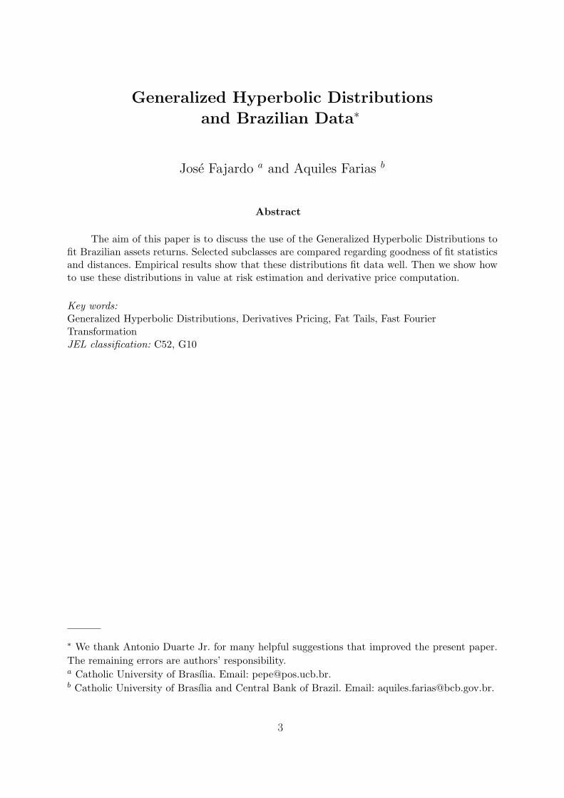
In table 2 we have the estimated parameters and the log-likelihood value. All samples but

Cemig have asymmetric distributions estimations since β is different from 0. The same

10

samples were submitted to Hyp software Blæsild and Sørensen (1992) and the results were

equivalent.

Table 2. Estimated parameters of Hyperbolic subclass (λ = 1) and log-likelihood values.

Sample α β δ µ Log-Likelihood

Bbas4 41.5931 3.896030 0.0130788 -0.005505 3512.08

Bbdc4 47.5455 -0.000629 2.11E-08 -1.45E-09 3984.49

Brdt4 51.7172 4.103200 0.011870 -0.003185 3925.06

Cmig4 43.3673 5.07E-07 0.0103856 0.000362 3677.76

Csna3 47.4118 0.008238 2.11E-08 3.84E-11 3976.50

Ebtp4 36.7618 3.808810 0.0196585 -0.00749485 1409.48

Elet6 41.1231 1.172670 0.0145371 -0.00120626 3522.58

Ibvsp 57.6958 -0.006950 0.00957707 0.00118714 4165.69

Itau4 49.9390 1.749500 2.02E-08 2.28E-09 4084.89

Petr4 45.7651 0.797027 0.010191 2.75E-05 3755.75

Tcsl4 35.5804 0.000417 0.032395 0.001370 1325.28

Tlpp4 41.7147 -0.005093 4.65E-07 1.34E-07 3753.45

Tnep4 34.9981 3.461250 0.0310437 -0.00540191 1314.64

Tnlp4 42.7018 0.002519 0.020710 0.000345821 1501.83

Vale5 48.7391 2.988860 0.00560929 -0.00170568 3955.42

In fig. 3, at the end of the paper, we have the Vale do Rio Doce (Vale5) Hyperbolic subclass

estimation compared to the Gaussian estimation and Empirical distribution. The figure

leads us to visually evaluate the better fit of Hyperbolic subclass.

The Hyperbolic subclass seems to better fit the leptokurtic behavior of the empirical

curve. To see the fitness of the tails of the distribution we refer to log-density graphic

4. We can see again that, visually, the Hyperbolic distribution is closer to the empirical

distribution.

11

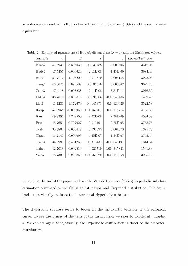
5.2 Normal Inverse Gaussian subclass

The Normal Inverse Gaussian Distribution (NIG) (λ = −0.5) has been very used and

for German data (Prause, 1999) it presented better fit than Hyperbolic. The estimated

parameters and the log-likelihood values are in table 3.

Table 3. Estimated NIG parameters.

Sample α β δ µ Log-Likelihood

Bbas4 26.1863 3.3516300 0.0356299 -0.00485126 3512.65

Bbdc4 25.2340 0.0026819 0.0234468 7.6154E-05 3978.71

Brdt4 36.7793 3.7894200 0.0324629 -0.00289173 3922.97

Cmig4 27.0195 0.0008486 0.0326901 0.00031385 3681.63

Csna3 25.3325 2.4752800 0.0235746 -0.00149070 3949.86

Ebtp4 22.8770 3.7054400 0.0424283 -0.00746229 1412.84

Elet6 23.6626 0.0033938 0.0343010 2.6479E-05 3532.29

Ibvsp 31.9096 -0.0034818 0.0232961 0.00122217 4178.17

Itau4 30.7352 0.0014784 0.0248846 0.00081258 4065.40

Petr4 25.3411 0.0008998 0.0284943 0.00067786 3764.37

Tcsl4 24.5055 -0.0002506 0.0555594 0.00123335 1327.02

Tlpp4 20.3812 0.0037757 0.0249410 0.00032556 3763.65

Tnep4 21.8374 0.0013490 0.0519268 0.00118522 1317.41

Tnlp4 26.2133 0.0009838 0.0384229 0.00038867 1505.29

Vale5 26.6233 0.0047853 0.0249197 9.7056E-05 3956.39

In fig. 5 we have the density graphics, while in fig. 6 we show the log-density graphics of

Vale do Rio Doce asset. Graphically we can not see much difference between Hyperbolic

and NIG distributions, but both seem better than Normal. The χ2− test of NIG are in

table 9.

5.3 Generalized Hyperbolic

A GHD is obtained through the λ freedom. Who first tested it empirically to financial

data was Prause (1999). Following him Raible (2000) published his work using the same

12

distributions.A big difficulty appeared when the parameters δ and µ tended simultane-

ously to zero (Raible, 2000). The numerical solution to this problem was to use specific

treatments to the case following Hanselman and Littlefield (2001) and Abramowitz and

Stegun (1968).

In Brazil they have never been used since Fajardo et al. (2001) only fit the Hyperbolic

subclass. Table 4 contains the estimations parameters for all samples studied.

Table 4. Estimated GHD Parameters.Sample α β δ µ λ L-Likelihood

Bbas4 30.7740 3.52665 0.02946 -0.00507 -0.0492 3512.73

Bbdc4 47.5455 -0.00063 2.1E-08 -1.4E-09 1 3984.49

Brdt4 56.4667 3.44169 0.00259 -0.00259 1.4012 3926.68

Cmig4 1.4142 0.74908 0.05150 -0.00038 -2.0600 3685.43

Csna3 46.1510 0.00941 2.2E-08 4.7E-11 0.6910 3987.52

Ebtp4 3.4315 3.43159 0.06704 -0.00708 -2.1773 1415.64

Elet6 1.4142 0.01203 0.05244 8.7E-05 -1.8987 3539.06

Ibvsp 1.7102 -1.66835 0.03574 0.00199 -1.8280 4186.31

Itau4 49.9390 1.74950 2.0E-08 2.3E-09 1 4084.89

Petr4 7.0668 0.48481 0.04163 0.00032 -1.6241 3767.41

Tcsl4 1.4142 -3.3E-06 0.08609 0.00114 -2.6210 1329.64

Tlpp4 6.8768 0.49049 0.03588 2.3E-05 -1.3333 3766.28

Tnep4 2.2126 2.21267 0.07857 -0.00280 -2.2980 1323.66

Tnlp4 1.4142 0.00208 0.05897 0.00045 -2.1536 1508.22

Vale5 25.2540 2.61339 0.02645 -0.00146 -0.6274 3958.47

As desired, the GHD estimations had higher log-likelihood values than its subclass, but

in Bradesco and Itau Samples where it is equal. The major samples had λ between -0.62

e -2.62 that is similar to the results obtained by Prause (1999). In figs. 2 and 7 we have

the density and log-density graphics.

13

−0.1 −0.05 0 0.05 0.1 0.150

50

100

150

200

250

300

350

400

Log−Returns

Den

sity

EmpiricNormalHyperbolicNIGGH

Fig. 2. Vale do Rio Doce Densities: Empiric x Hyperbolic x Normal x NIG x GH

6 Testing Goodness of Fit

In this section we test the goodness of fit, to this end we use the following tests and

distances:

• χ2 test: this test was used by Eberlein and Keller (1995) and Fajardo et al. (2001).

This test is not recommendable for evaluating continuous distributions (see Press et

al. (1992)), on the other hand Blæsild and Sørensen (1992) report that although the

chi-square test tends to reject statistical test for large samples, our tests do not report

that fact (table 8). This fact is due to the particular behavior of Brazilian market.

• Kolmogorov distance: this test is more suitable than chi-square test for continuous

distributions. Its expression is given by:

KS = maxx∈R

|Femp(x)− Fest(x)| (10)

• Kuiper distance: this is another distance evaluation used to test goodness of fit of

continuous distributions. The main difference between Kuiper and Kolmogorov distance

is that the first consider upper differences different from lower differences and in the

late all distances are considered equally. Its expression is given by:

14

KP = maxx∈R

{Femp(x)− Fest(x)}+ maxx∈R

{Fest(x)− Femp(x)} (11)

• Anderson & Darling distance: a third distance evaluation used was the Anderson &

Darling distance (12). The main difference between it and Kolmogorov’s distance is

that the first pays more attention to tail distances (Hurst et al., 1995).

AD = maxx∈R

|Femp(x)− Fest(x)|√Fest(x)(1− Fest(x))

(12)

Following we present the results obtained with each test.

6.1 Chi-Square Test

We present the Chi-Square test for GHD and the test for the Hyperbolic and NIG

subclasses are presented in tables 8 and 9 at the end of the paper.

Table 5. χ2−test for the GHD

Sample Statistic P-Value Degrees of Freedom

Bbas4 23.6516 0.0876783 15

Bbdc4 34.1268 0.000902191 14

Brdt4 66.2152 2.01218E-08 21

Cmig4 21.2875 0.165019 15

Csna3 141.597 0 19

Ebtp4 13.6279 0.341022 11

Elet6 21.383 0.268148 17

Ibvsp 13.5203 0.511037 13

Itau4 32.5035 0.0819379 22

Petr4 15.3088 0.718927 18

Tcsl4 18.9641 0.162971 13

Tlpp4 22.5389 0.0840841 14

Tnep4 13.3699 0.522905 13

Tnlp4 16.5175 0.225828 12

Vale5 16.1775 0.462554 15

15

From table 5 we observe that with 5% of significance level we can not reject the null

hypothesis of GHD behavior for 12 assets, in the NIG case we can not reject the null

hypothesis in 11 assets and in the Hyperbolic subclass case we can not reject the null

hypothesis in 9 assets.

6.2 Kolmogorov Distance

We present in table 6 the Kolmogorov distances of the NIG, Hyperbolic and GH distribu-

tions. In the Gh case all samples but CSNA3 can not be rejected using 1% of significance

using Kolmogorov test and Ibovespa index got a P-value of 99.69%.

Table 6. Kolmogorov distances.

Sample Normal Hyperbolic NIG GH

KS KS P-Value KS P-Value KS P-Value

Bbas4 0.0585 0.0202 0.4446 0.0252 0.1938 0.0236 0.2611

Bbdc4 0.0682 0.0279 0.1112 0.0282 0.1052 0.0279 0.1112

Brdt4 0.0505 0.0240 0.2380 0.0303 0.0664 0.0252 0.1914

Cmig4 0.0559 0.0238 0.2440 0.0256 0.1779 0.0270 0.1354

Csna3 0.0744 0.0355 0.0192 0.0382 0.0092 0.0501 0.0002

Ebtp4 0.0699 0.0253 0.6818 0.0259 0.6537 0.0234 0.7694

Elet6 0.0598 0.0150 0.7968 0.0123 0.9415 0.0103 0.9897

Ibvsp 0.0661 0.0208 0.3967 0.0166 0.6833 0.0093 0.9970

Itau4 0.0681 0.0347 0.0233 0.0340 0.0276 0.0347 0.0233

Petr4 0.0640 0.0142 0.8526 0.0133 0.8993 0.0126 0.9294

Tcsl4 0.0458 0.0220 0.8307 0.0236 0.7594 0.0253 0.6823

Tlpp4 0.0784 0.0193 0.4924 0.0225 0.3062 0.0233 0.2691

Tnep4 0.0584 0.0187 0.9405 0.0239 0.7456 0.0219 0.8342

Tnlp4 0.0597 0.0178 0.9615 0.0188 0.9387 0.0178 0.9616

Vale5 0.0751 0.0099 0.9931 0.0121 0.9497 0.0108 0.9813

16

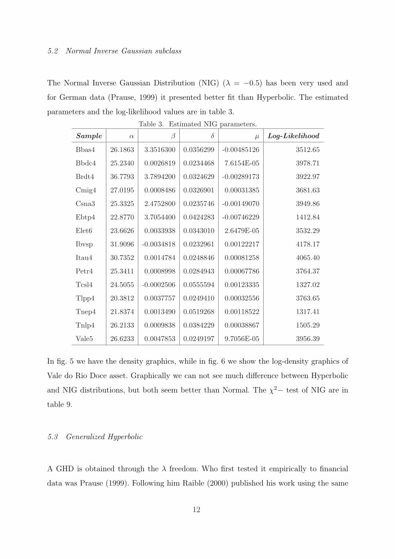
6.3 Kuiper Distance

In table 10, at the end of the paper, we have the Kuiper distances of Hyperbolic subclass,

NIG and GH distributions. In Hyperbolic case we verify that 13 samples can not be

rejected using 1% of significance. In NIG case we can not reject the null hypothesis for 12

samples (1% of significance). The Kuiper test rejects with 1% only two samples, in GH

case, but even in the rejected samples the distance evaluated in the above estimates are

smaller then Normal distances.

6.4 Anderson & Darling Distance

We present the results in table 11. We observe that this distance clearly shows the

difference of fitness in the distributions tails. Analyzing the distances in comparison with

the Hyperbolic we can deduce that the NIG is better as far as tail fitness is concerned.

The Anderson and Darling test shows that GHD fit better in tails than Hyperbolic and

are similar to NIG distances.

7 Derivative Pricing

Since Black and Scholes (1973), closed formula for European calls have been analyzed, but

these models assume that the underlying distribution of the log-returns is Normal. More

recently Prause (1999) and Raible (2000) presented the Levy Generalized Hyperbolic

process, where they assume that the log-returns of assets follow a GHD or one of its

subclasses. Now we price European calls with Brazilian assets.

7.1 Generalized Hyperbolic Distributions Convolution

The first step on derivative pricing is calculating the GHD convolution, except for NIG

subclass. Such subclass has the closed formula in (13).

17

NIG∗t(x; α, β, δ, µ) = NIG(x; α, β, tδ, tµ) (13)

To solve the convolution problem using other subclasses we use Fourier transforms. The

characteristic function is obtained using a Fourier transform and a transformed function

multiplication is similar to the original function convolution, so we follow these steps:

1 - Apply Fourier transform in estimated GHD density.

2 - Multiply this transform by as many convolutions as we need.

3 - Apply the Inverse Fourier transform to obtain the GHD with t-fold convolution.

To easy calculation we use symmetric and centered distribution (β, µ = 0) to guarantee

that the functions are real (Press et al., 1992). So, we follow Prause (1999) and find a

GHD as a function of a centered and symmetric GHD. This function is in (14).

GH∗t(x; α, β, δ, µ, λ) =eβx

M t0(β)

gh∗t(x− µt; λ, α, 0, δ, 0) (14)

Where M t0(β) represents the moment generating function with parameter β = 0, powered

to t and evaluated in β as an argument. Then we apply the fourier transform in centered

and symmetric GHD, obtaining (15). Then we should apply the inverse Fourier transform,

but it doesn’t have an analytical solution.

GH∗t(x; α, 0, δ, 0, λ) =1

π

∫ ∞

0cos(ux)ϕ(u; α, δλ)tdu (15)

To solve this kind of problem we use the Cooley and Tukey (1965) algorithm called Fast

Fourier Transformation (FFT). We refer to Brigham (1988) and Press et al. (1992) for

details on this algorithm applications.

The FFT calculates the Fourier transform and the inverse Fourier transform in an efficient

way. The main concern here is related to variable transformations from frequency to time

domain 3 .

3 To details about this variable transformation and a Matlab example we refer to Hanselman

18

After FFT application we have the density of symmetric and centered with t-fold convo-

lution. To get the desired density we use (14).

7.2 Option Pricing Using Esscher Transforms

To price options with underlying assets following diffusions driven by Levy processes we

have to find an Equivalent martingale measure. Esscher (1932) presented a transform that

was used by Gerber and Shiu (1994) for derivative pricing.

In GHD case this transformation to risk-neutral world is in (16).

GH∗t,ϑ(x; α, β, δ, µ, λ) =eϑx

M t(ϑ)GH∗t(x; α, β, δ, µ, λ) (16)

To find the ϑ parameter we have to solve (17).

r = logM(ϑ + 1)

M(ϑ)(17)

Where r is the risk free interest rate in the same period of estimated data and M is the

moment generating function. The solution of this equation is obtained through numerical

optimization.

The last step is to obtain the European Call prices. In this step we follow Keller (1997).

CGH = S0

∫ ∞

log KS0

GH∗t,ϑ+1(x)dx− e−rtK∫ ∞

log KS0

GH∗t,ϑ(x)dx (18)

where K is the strike price and S0 is the stock price. In this case the Put-Call parity is

valid, in order to calculate a Put price we use (19).

PGH = CGH − S0 + e−rtK (19)

and Littlefield (2001).

19

7.3 Empirical Evidence

In figs. 8, 9 e 10 we have graphics with the Vale do Rio Doce Call behavior when changing

certain parameters and, as expected, the major sensibility of Call prices are when the

Option is at the money. Then we do comparative analysis of GHD call prices and Black

and Scholes (1973) call prices of this asset. We obtain figs. 11, 12 e 13 that contain the

difference between the prices. We can see clearly the desired W-Shape.

8 Value At Risk

The Value At Risk represents the worst loss, given a time period and a probability in

market normal conditions (Jorion, 1997). In this section we briefly explore the parametric

VaR using Normal and GHD as asset log-returns distributions. In fig. 14 we have the

VaR graphics for different probability levels, and we can see that the GHD get closer to

empirical probability.

Another way to test the efficiency of VaR models is Back Testing (Jorion, 1997) and we

considered a portfolio with one asset only (Vale do Rio Doce) with an initial portfolio value

of R$ 1,00. The initial sample used consisted of 252 observations, starting in 07/01/1994,

reaching 1590 out of sample tests. Each day the VaR for 1 trading day holding period

with 1% of probability was calculated. If the real loss were bigger then the predicted we

consider this one exception. Then we aggregated this observation and repeated the steps

to another day.

The results of the test are in table 7, that brings the number of exceptions and the Kupiec

(1995) test P-Value whose null hypothesis is “The two probabilities are equal”.

This method of evaluation has as a major criticism the fact that it measures exceptions

but do not measures the size of error, but we can see, only by using it, that the GHD

represents better risk measures.

20

Table 7. Exceptions and Kupiec-test p-value.

Distribution Exceptions Probability P-Value

Normal 21 0.013208 0.22

Hyperbolic 17 0.010692 0.78

N.I.G. 16 0.010063 0.98

G.H. 16 0.010063 0.98

9 Conclusions

In this paper we evaluated the goodness of fit of Generalized Hyperbolic Distributions to

Brazilian log-return assets and showed that they are better to model asset log-returns than

Gaussian distribution. Then we used Fast Fourier Transformation and Esscher transforms

to option pricing and we compensate a part of Black and Scholes (1973) mispricing. In the

last section we calculated VaR measures and showed that GHD improve risk measures.

The main limitations of the model are the non-market parameters, as volatility is in

Normal distributions, the computational effort to parameter estimation and derivative

pricing and finally the utilization of numerical calculus that require attention in precision

determination. It is important to observe the trade-off between the use of a subclass or the

Generalized class. The use of Hyperbolic subclass provides faster parameter estimation

and the NIG easies the derivative pricing (since it is closed under convolution).

Last, we have shown many empirical evidence in favor of the use of this GHD distributions

to fit Brazilian data, indeed the same analysis can be carried on to analyze other Latin

American markets.

References

Abramowitz, M. and I. A. Stegun (1968), “Handbook of Mathematical Functions”, Dover

Publ., New York.

Barndorff-Nielsen, O. (1977), “Exponentially Decreasing Distributions for the Logarithm

of Particle Size” , Proceedings of the Royal Society London A, 353, 401-419.

21

Barndorff-Nielsen, O. (1978), “Hyperbolic Distributions and Distributions on Hyperbo-

lae”, Scandinavian Journal of Statistics, 5, 151-157.

Barndorff-Nielsen, O. (1997), “Normal Inverse Gaussian Distributions and Stochastic

Volatility Modelling”, Scandinavian Journal of Statistics, 24, 1-13.

Barndorff-Nielsen, O. (1998), “Processes of Normal Inverse Gaussian Type”, Finance &

Stochastics, 2, 41-68.

Barndorff-Nielsen, O. E. and P. Blæsild, “Hyperbolic distributions and ramifications:

Contributions to theory and application” In C. Taillie, G. Patil, and B. Baldessari

(Eds.), Statistical Distributions in Scientific Work, Volume 4, pp. 19-44. Dordrecht:

Reidel.

Black, F. and M. Scholes (1973), “The Pricing of Options and Corporate Liabilities”,

Journal of Political Economy, 81, 3, 637-654.

Blæsild, P. and M. Sørensen (1992), “Hyp a Computer Program for Analyzing Data by

Means of the Hyperbolic Distribution”, Department of Theoretical Statistics, Aarhus

University Research Report, 248.

Brigham, E. O. (1988), “The Fast Fourier Transform and Its Applications”, Prentice Hall,

New Jersey.

Cooley, J. and J. Tukey (1965), “An Algorithm For The Machine Calculation Of Complex

Fourier Series”, Mathematics of Computations, 19, 90, 297-301.

Duarte J., A.M. and Mendez, B.V.M. (1999), “Robust Estimation for ARCH Models”.

Brazilian Review of Econometrics, vol 19, No. 139-180.

Eberlein, E. (2000), “Mastering Risk”, Prentice Hall.

Eberlein, E. and U. Keller (1995), “Hyperbolic Distributions in Finance”, Bernoulli, 1995,

1, 281-299.

Esscher, F. (1932), “On the probability function in the collective theory of risk”,

Skandinavisk Aktuarietidskrift, 15, 175-195.

Fajardo, J., A. Schuschny e A. Silva (2001), “Processos de Levy e o Mercado Brasileiro”,

Catholic University of Brasilia, Working Paper. Forthcoming Brazilian Review of

Econometrics.

Gerber, H. U. and E. S. W. Shiu (1994), “Option pricing by Esscher-transforms”,

Transactions of the Society of Actuaries, 46, 99-191 With Discussion.

22

Hanselman, D. C. and B. Littlefield (2001), “Mastering Matlab 6 - A Comprehensive

Tutorial and Reference”, Prentice Hall.

Hurst, S. R., E. Platen, and S. T. Rachev (1995), “Option pricing for asset returns driven

by subordinated processes”, Working Paper, The Australian National University.

Issler, J.V. (1999). “Estimating and Forecasting the Volatility of Brazilian Finance Series

Using ARCH Models”. Brazilian Review of Econometrics, vol 19, No. 1, 5-56.

Jorion, P. (1997), Value at Risk: The New Benchmark for Controlling Market Risk,

McGraw-Hill.

Keller, U. (1997), “Realistic modelling of financial derivatives”, University of Freiburg,

Doctoral Thesis.

Kupiec, P. H. (1995), “Techniques for Verifying the Accuracy of Risk Measurement

Models”, Journal of Derivatives, Winter, 73-84.

Mandelbrot, B. (1963), “The variation of certain speculative prices”,Journal of Business,

36, 394-419.

Mazuchelli, J. and Migon, H. S. (1999), “Modelos GARCH Bayesianos: Metodos

Aproximados e Aplicacoes”. Brazilian Review of Econometrics, vol 19, No. 1, 111-138.

Nelder, J. and R. Mead (1965), “A Simplex Method for Function Minimization”, Computer

Journal, 7, 308-313.

Pereira, P.L.V., Hotta, L.K., Souza, L.A.R. and Almeida, N.M.C.G.(1999). “Alternative

Models to Extract Asset Volatility: A Comparative Study”. Brazilian Review of

Econometrics, vol 19, No. 1, 57-109.

Prause, K. (1999), “The generalized hyperbolic model: Estimation, financial derivatives,

and risk measures”, University of Freiburg, Doctoral Thesis.

Press , W., S. Teukolsky, W. Vetterling, and B. Flannery (1992), “ Numerical Recipes in

C”, Cambridge University Press, Cambridge.

Raible, S. (2000), “Levy Processes in Finance: Theory, Numerics, and Empirical Facts”,

University of Freiburg, Doctoral Thesis.

Rydberg, T. (1997), “Why Financial Data are Interesting to Statisticians”, Centre for

Analytical Finance, Aarhus University Working Paper 5.

23

Table 8. Hyperbolic χ2 tests.

Sample Statistic P-Value Degrees of Freedom

Bbas4 23.4443 0.0930294 15

Bbdc4 34.1268 0.0009022 14

Brdt4 70.7405 1.308E-09 21

Cmig4 21.3939 0.1607190 15

Csna3 55.3857 1.690E-05 22

Ebtp4 13.9941 0.3941480 12

Elet6 34.1289 0.0062942 17

Ibvsp 34.4265 0.0007819 14

Itau4 32.5035 0.0819379 22

Petr4 25.8397 0.1694790 19

Tcsl4 20.6518 0.1431640 14

Tlpp4 34.9870 0.0005964 14

Tnep4 16.6171 0.2871920 13

Tnlp4 19.5150 0.1404500 13

Vale5 12.2598 0.6807120 14

24

Table 9. NIG χ2 tests.

Sample Statistic P-Value Degrees of Freedom

Bbas4 24.3353 0.071753 15

Bbdc4 30.8658 0.003959 14

Brdt4 80.2756 2.64E-12 21

Cmig4 21.2789 0.165371 15

Csna3 92.3705 2.44E-15 22

Ebtp4 14.3936 0.364241 12

Elet6 26.8696 0.071477 17

Ibvsp 23.5482 0.061650 14

Itau4 56.8740 3.51E-06 21

Petr4 18.5013 0.575688 19

Tcsl4 20.2143 0.160487 14

Tlpp4 21.0947 0.127084 14

Tnep4 19.8779 0.126934 13

Tnlp4 18.0578 0.205481 13

Vale5 16.9344 0.337203 14

25

Table 10. Kuiper distances.

SampleNormal Hyperbolic NIG GH

KP KP P-Value KP P-Value KP P-Value

Bbas4 0.1133 0.0332 0.2495 0.0391 0.0742 0.0370 0.1187

Bbdc4 0.1299 0.0462 0.0109 0.0496 0.0038 0.0462 0.0109

Brdt4 0.0969 0.0413 0.0419 0.0450 0.0152 0.0414 0.0406

Cmig4 0.1022 0.0352 0.1662 0.0392 0.0694 0.0419 0.0356

Csna3 0.1299 0.0677 0.0000 0.0754 0.0000 0.1000 1 E-14

Ebtp4 0.1259 0.0442 0.4531 0.0452 0.4124 0.0393 0.6615

Elet6 0.1190 0.0290 0.4651 0.0228 0.8434 0.0188 0.9754

Ibvsp 0.1306 0.0280 0.5278 0.0253 0.6975 0.0172 0.9924

Itau4 0.1164 0.0470 0.0086 0.0554 0.0005 0.0470 0.0086

Petr4 0.1225 0.0254 0.6948 0.0259 0.6648 0.0226 0.8574

Tcsl4 0.0839 0.0418 0.5533 0.0431 0.4980 0.0424 0.5260

Tlpp4 0.1549 0.0351 0.1668 0.0363 0.1309 0.0349 0.1748

Tnep4 0.1101 0.0364 0.7757 0.0448 0.4274 0.0412 0.5768

Tnlp4 0.1177 0.0349 0.8357 0.0375 0.7370 0.0336 0.8761

Vale5 0.1332 0.0191 0.9701 0.0236 0.8020 0.0186 0.9782

26

Table 11. Anderson & Darling Distance

Sample Normal Hyperbolic NIG GH

Bbas4 137028000 3.14961 0.809321 1.19094

Bbdc4 51579.5 0.128786 0.168094 0.12879

Brdt4 485.583 0.21863 0.147332 0.24283

Cmig4 10296 0.451259 0.221778 0.07197

Csna3 7.14072 0.071032 0.0764042 0.1546

Ebtp4 118781 2.27445 0.509757 0.0762

Elet6 51495.5 0.473038 0.183155 0.08368

Ibvsp 72825.7 2.68092 0.371791 0.0831

Itau4 4.6648 0.075514 0.0680073 0.07551

Petr4 67.0476 0.167398 0.0720301 0.04054

Tcsl4 1849990 2.86085 1.08921 0.22114

Tlpp4 51523.5 0.517512 0.304372 0.05785

Tnep4 305.017 0.769552 0.205116 0.17429

Tnlp4 119529 5.94561 1.21541 0.17534

Vale5 51523.5 4.7077 0.74826 0.39979

−0.1 −0.05 0 0.05 0.1 0.150

50

100

150

200

250

300

350

400

Log−Returns

Den

sity

EmpiricNormalHyperbolic

Fig. 3. Vale densities: Empiric x Hyperbolic x Normal

27

−0.1 −0.05 0 0.05 0.1 0.1510

0

101

102

Log−Returns

Log−

Den

sity

EmpiricNormalHyperbolic

Fig. 4. Vale Log-densities: Empiric x Hyperbolic x Normal

−0.1 −0.05 0 0.05 0.1 0.150

50

100

150

200

250

300

350

400

Log−Returns

Den

sity

EmpiricNormalHyperbolicNIG

Fig. 5. Vale do Rio Doce Densities: Empiric x Hyperbolic x Normal x NIG

28

−0.1 −0.05 0 0.05 0.1 0.1510

0

101

102

Log−Returns

Log−

Den

sity

EmpiricNormalHyperbolicNIG

Fig. 6. Vale do Rio Doce Log-Densities: Empiric x Hyperbolic x Normal x NIG

−0.1 −0.05 0 0.05 0.1 0.1510

0

101

102

Log−Returns

Log−

Den

sity

EmpiricNormalHyperbolicNIGGH

Fig. 7. Vale do Rio Doce Log-Densities: Empiric x Hyperbolic x Normal x NIG x GH

29

40

45

50

55

60 0

5

10

15

20

0

2

4

6

8

10

12

Mat

urity

Strike Price

Cal

l Pric

e

Fig. 8. Vale do Rio Doce Call price with S0 = 50 and risk free interest rate 19% using Hyperbolic

subclass.

40

45

50

55

60 0

5

10

15

20

0

2

4

6

8

10

12

Mat

urity

Strike Price

Cal

l Pric

e

Fig. 9. Vale do Rio Doce Call price with S0 = 50 and risk free interest rate 19% using Generalized

Hyperbolic distribution.

30

40

45

50

55

60 0

5

10

15

20

0

2

4

6

8

10

12

Mat

urity

Strike Price

Cal

l Pric

e

Fig. 10. Vale do Rio Doce Call price with S0 = 50 and risk free interest rate 19% using Normal

Inverse Gaussian Distribution.

40

45

50

55

60

0

5

10

15

20−0.02

0

0.02

0.04

0.06

0.08

0.1

0.12

0.14

0.16

Strike Price

Maturity

BS

− H

yper

bolic

Fig. 11. Black and Scholes minus Hyperbolic Vale do Rio Doce Call prices for various maturities

and strike prices .

31

40

45

50

55

60

0

5

10

15

20−0.04

−0.02

0

0.02

0.04

0.06

0.08

0.1

0.12

Strike Price

Maturity

BS

− N

IG

Fig. 12. Black and Scholes minus NIG Vale do Rio Doce Call prices for various maturities and

strike prices.

40

45

50

55

60

0

5

10

15

20−0.04

−0.02

0

0.02

0.04

0.06

0.08

0.1

0.12

Strike Price

Maturity

BS

− G

H

Fig. 13. Black and Scholes minus GHD Vale do Rio Doce Call prices for various maturities and

strike prices.

32

0 0.01 0.02 0.03 0.04 0.05 0.06 0.07 0.08 0.09 0.10.03

0.04

0.05

0.06

0.07

0.08

0.09

0.1

0.11

Probability

Val

ue A

t Ris

k

EmpiricNormalNIGHYPGH

Fig. 14. Value At Risk of portfolio consisting of Vale do Rio Doce assets for different probabilities

with 1 trading day holding period and the portfolio value of R$ 1,00.

33

34

Banco Central do Brasil

Trabalhos para Discussão Os Trabalhos para Discussão podem ser acessados na internet, no formato PDF,

no endereço: http://www.bc.gov.br

Working Paper Series

Working Papers in PDF format can be downloaded from: http://www.bc.gov.br

1 Implementing Inflation Targeting in Brazil

Joel Bogdanski, Alexandre Antonio Tombini and Sérgio Ribeiro da Costa Werlang

July/2000

2 Política Monetária e Supervisão do Sistema Financeiro Nacional no Banco Central do Brasil Eduardo Lundberg Monetary Policy and Banking Supervision Functions on the Central Bank Eduardo Lundberg

Jul/2000

July/2000

3 Private Sector Participation: a Theoretical Justification of the Brazilian Position Sérgio Ribeiro da Costa Werlang

July/2000

4 An Information Theory Approach to the Aggregation of Log-Linear Models Pedro H. Albuquerque

July/2000

5 The Pass-Through from Depreciation to Inflation: a Panel Study Ilan Goldfajn and Sérgio Ribeiro da Costa Werlang

July/2000

6 Optimal Interest Rate Rules in Inflation Targeting Frameworks José Alvaro Rodrigues Neto, Fabio Araújo and Marta Baltar J. Moreira

July/2000

7 Leading Indicators of Inflation for Brazil Marcelle Chauvet

Set/2000

8 The Correlation Matrix of the Brazilian Central Bank’s Standard Model for Interest Rate Market Risk José Alvaro Rodrigues Neto

Set/2000

9 Estimating Exchange Market Pressure and Intervention Activity Emanuel-Werner Kohlscheen

Nov/2000

10 Análise do Financiamento Externo a uma Pequena Economia Aplicação da Teoria do Prêmio Monetário ao Caso Brasileiro: 1991–1998 Carlos Hamilton Vasconcelos Araújo e Renato Galvão Flôres Júnior

Mar/2001

11 A Note on the Efficient Estimation of Inflation in Brazil Michael F. Bryan and Stephen G. Cecchetti

Mar/2001

35

12 A Test of Competition in Brazilian Banking Márcio I. Nakane

Mar/2001

13 Modelos de Previsão de Insolvência Bancária no Brasil Marcio Magalhães Janot

Mar/2001

14 Evaluating Core Inflation Measures for Brazil Francisco Marcos Rodrigues Figueiredo

Mar/2001

15 Is It Worth Tracking Dollar/Real Implied Volatility? Sandro Canesso de Andrade and Benjamin Miranda Tabak

Mar/2001

16 Avaliação das Projeções do Modelo Estrutural do Banco Central do Brasil Para a Taxa de Variação do IPCA Sergio Afonso Lago Alves Evaluation of the Central Bank of Brazil Structural Model’s Inflation Forecasts in an Inflation Targeting Framework Sergio Afonso Lago Alves

Mar/2001

July/2001

17 Estimando o Produto Potencial Brasileiro: uma Abordagem de Função de Produção Tito Nícias Teixeira da Silva Filho Estimating Brazilian Potential Output: a Production Function Approach Tito Nícias Teixeira da Silva Filho

Abr/2001

Aug/2002

18 A Simple Model for Inflation Targeting in Brazil Paulo Springer de Freitas and Marcelo Kfoury Muinhos

Apr/2001

19 Uncovered Interest Parity with Fundamentals: a Brazilian Exchange Rate Forecast Model Marcelo Kfoury Muinhos, Paulo Springer de Freitas and Fabio Araújo

May/2001

20 Credit Channel without the LM Curve Victorio Y. T. Chu and Márcio I. Nakane

May/2001

21 Os Impactos Econômicos da CPMF: Teoria e Evidência Pedro H. Albuquerque

Jun/2001

22 Decentralized Portfolio Management Paulo Coutinho and Benjamin Miranda Tabak

June/2001

23 Os Efeitos da CPMF sobre a Intermediação Financeira Sérgio Mikio Koyama e Márcio I. Nakane

Jul/2001

24 Inflation Targeting in Brazil: Shocks, Backward-Looking Prices, and IMF Conditionality Joel Bogdanski, Paulo Springer de Freitas, Ilan Goldfajn and Alexandre Antonio Tombini

Aug/2001

25 Inflation Targeting in Brazil: Reviewing Two Years of Monetary Policy 1999/00 Pedro Fachada

Aug/2001

36

26 Inflation Targeting in an Open Financially Integrated Emerging Economy: the Case of Brazil Marcelo Kfoury Muinhos

Aug/2001

27

Complementaridade e Fungibilidade dos Fluxos de Capitais Internacionais Carlos Hamilton Vasconcelos Araújo e Renato Galvão Flôres Júnior

Set/2001

28

Regras Monetárias e Dinâmica Macroeconômica no Brasil: uma Abordagem de Expectativas Racionais Marco Antonio Bonomo e Ricardo D. Brito

Nov/2001

29 Using a Money Demand Model to Evaluate Monetary Policies in Brazil Pedro H. Albuquerque and Solange Gouvêa

Nov/2001

30 Testing the Expectations Hypothesis in the Brazilian Term Structure of Interest Rates Benjamin Miranda Tabak and Sandro Canesso de Andrade

Nov/2001

31 Algumas Considerações sobre a Sazonalidade no IPCA Francisco Marcos R. Figueiredo e Roberta Blass Staub

Nov/2001

32 Crises Cambiais e Ataques Especulativos no Brasil Mauro Costa Miranda

Nov/2001

33 Monetary Policy and Inflation in Brazil (1975-2000): a VAR Estimation André Minella

Nov/2001

34 Constrained Discretion and Collective Action Problems: Reflections on the Resolution of International Financial Crises Arminio Fraga and Daniel Luiz Gleizer

Nov/2001

35 Uma Definição Operacional de Estabilidade de Preços Tito Nícias Teixeira da Silva Filho

Dez/2001

36 Can Emerging Markets Float? Should They Inflation Target? Barry Eichengreen

Feb/2002

37 Monetary Policy in Brazil: Remarks on the Inflation Targeting Regime, Public Debt Management and Open Market Operations Luiz Fernando Figueiredo, Pedro Fachada and Sérgio Goldenstein

Mar/2002

38 Volatilidade Implícita e Antecipação de Eventos de Stress: um Teste para o Mercado Brasileiro Frederico Pechir Gomes

Mar/2002

39 Opções sobre Dólar Comercial e Expectativas a Respeito do Comportamento da Taxa de Câmbio Paulo Castor de Castro

Mar/2002

40 Speculative Attacks on Debts, Dollarization and Optimum Currency Areas Aloisio Araujo and Márcia Leon

Abr/2002

41 Mudanças de Regime no Câmbio Brasileiro Carlos Hamilton V. Araújo e Getúlio B. da Silveira Filho

Jun/2002

37

42 Modelo Estrutural com Setor Externo: Endogenização do Prêmio de Risco e do Câmbio Marcelo Kfoury Muinhos, Sérgio Afonso Lago Alves e Gil Riella

Jun/2002

43 The Effects of the Brazilian ADRs Program on Domestic Market Efficiency Benjamin Miranda Tabak and Eduardo José Araújo Lima

June/2002

44 Estrutura Competitiva, Produtividade Industrial e Liberação Comercial no Brasil Pedro Cavalcanti Ferreira e Osmani Teixeira de Carvalho Guillén

Jun/2002

45 Optimal Monetary Policy, Gains from Commitment, and Inflation Persistence André Minella

Aug/2002

46 The Determinants of Bank Interest Spread in Brazil Tarsila Segalla Afanasieff, Priscilla Maria Villa Lhacer and Márcio I. Nakane

Aug/2002

47 Indicadores Derivados de Agregados Monetários Fernando de Aquino Fonseca Neto e José Albuquerque Júnior

Sep/2002

48 Should Government Smooth Exchange Rate Risk? Ilan Goldfajn and Marcos Antonio Silveira

Sep/2002

49 Desenvolvimento do Sistema Financeiro e Crescimento Econômico no Brasil: Evidências de Causalidade Orlando Carneiro de Matos

Set/2002

50 Macroeconomic Coordination and Inflation Targeting in a Two-Country Model Eui Jung Chang, Marcelo Kfoury Muinhos and Joanílio Rodolpho Teixeira

Sep/2002

51 Credit Channel with Sovereign Credit Risk: an Empirical Test Victorio Yi Tson Chu

Sep/2002