University of South Florida University of South Florida

Scholar Commons Scholar Commons

Graduate Theses and Dissertations Graduate School

2011

Simplified Methodology for Designing Parabolic Trough Solar Simplified Methodology for Designing Parabolic Trough Solar

Power Plants Power Plants

Ricardo Vasquez Padilla University of South Florida, rsvasque@mail.usf.edu

Follow this and additional works at: https://scholarcommons.usf.edu/etd

Part of the American Studies Commons, Engineering Commons, and the Oil, Gas, and Energy

Commons

Scholar Commons Citation Scholar Commons Citation Vasquez Padilla, Ricardo, "Simplified Methodology for Designing Parabolic Trough Solar Power Plants" (2011). Graduate Theses and Dissertations. https://scholarcommons.usf.edu/etd/3390

This Dissertation is brought to you for free and open access by the Graduate School at Scholar Commons. It has been accepted for inclusion in Graduate Theses and Dissertations by an authorized administrator of Scholar Commons. For more information, please contact scholarcommons@usf.edu.

Simplified Methodology for Designing Parabolic Trough Solar Power Plants

by

Ricardo Vasquez Padilla

A dissertation submitted in partial fulfillmentof the requirements for the degree of

Doctor of PhilosophyDepartment of Chemical and Biomedical Engineering

College of EngineeringUniversity of South Florida

Co-Major Professor: D. Yogi Goswami, Ph.D.Co-Major Professor: Elias Stefanakos, Ph.D.

Muhammad M. Rahman, Ph.D.John T. Wolan, Ph.D.Yuncheng You, Ph.D.

Date of Approval:April 4, 2011

Keywords: Solar radiation, Solar shading, Regenerative Rankine cycle, Levelized cost ofelectricity, Air cooled condensers

Copyright © 2011, Ricardo Vasquez Padilla

Dedication

Dedicated to Jehovah and my two loves: Jenni and Noah

Acknowledgements

I express my most sincere gratitude to my advisors, Dr. Yogi Goswami and Dr Ste-

fanakos for their guidance, patience, understanding and encouragement throughout this

work. I also like to thank the members of my committee, Drs. Muhammad Rahman, John

Wolan and Yuncheng You. Special thanks to Ms. Ginny Cosmides, Ms. Barbara Graham

and Mr. Charles Garretson who with their advice and kindness were great help during my

stay in the Clean Energy Research Center (CERC).

I would like to thank my friends Sesha, Saeb, June, Chennan, Antonio, Jamie, Kofi,

Yang and Gokmen, in the CERC, for their help and support, and the Universidad del Norte

for the economic support in my doctoral studies. I would also like to thank my friends:

Viviana, Homero, Henry, Paula Lezama, Sophia, Cesar, Paula Algarin, Pedro, Cecilia and

Mrs. Ena. I can not forget my friend Rolland who is no longer with us but will live forever

in my memories. Special acknowledge goes to Ms. Ana Rivera and Alondra for their

spiritual support and friendship. I would like to give special thanks to my mother, Nubia,

my father, Armando, and my aunt Sara, because they have always believed in me. Thanks

to my parents in law Santiago and Maria de Lourdes, without their help this dissertation

would not have been written. Finally, I would like to acknowledge Jehovah for giving

me strength in moments of weakness and my wife Jennifer and my son Noah for their

unwavering support and for being my inspiration.

Table of Contents

List of Tables iv

List of Figures viii

List of Symbols xv

Abstract xix

Chapter 1 Introduction 11.1 Literature Review 5

Chapter 2 Solar Radiation 92.1 Solar Angles 102.2 Hourly Solar Radiation Models 202.3 Single Axis Tracking 28

2.3.1 Horizontal Tracking Axis 302.4 Results 312.5 Solar Shading 362.6 Conclusions 48

Chapter 3 Heat Transfer Analysis of Parabolic Trough Solar Receiver 503.1 Introduction 503.2 Solar Receiver Model 53

3.2.1 Heat Transfer from Absorber to Heat Transfer Fluid 563.2.1.1 Circular Pipe 573.2.1.2 Concentric Annulus 60

3.2.2 Heat Transfer from Absorber to Glass Envelope 623.2.2.1 Vacuum in Annulus (P < 1 Torr) 633.2.2.2 Pressure in Annulus (P > 1 Torr) 653.2.2.3 Radiation Heat Transfer from Receiver to Enve-

lope 673.2.2.4 Heat Conduction Through Support Brackets 76

3.2.3 Heat Transfer from Glass Envelope to the Ambient 823.2.3.1 Heat Convection 843.2.3.2 Radiation Heat Transfer (Sky and Collector Sur-

face) 85

i

3.2.4 Solar Energy Absorption 903.3 Numerical Solution 973.4 Model Validation 1003.5 Results and Discussion 1033.6 Non-Linear Regression Heat Loss Model 1113.7 Conclusions 112

Chapter 4 Power Block 1144.1 Introduction 1144.2 Reheater and Superheater 1184.3 Boiler 1224.4 Preheater 1254.5 Closed Feedwater 1264.6 Open Feedwater (Deaerator) 1294.7 Turbine 1304.8 Pump 1344.9 Condenser 137

4.9.1 Cooling Tower 1384.9.1.1 Design Procedure 139

4.9.2 Cooling Tower Performance at Off Design Conditions 1444.9.3 Air Cooled Condensers 147

4.9.3.1 Design of the Air Cooled Condensers 1524.10 Net Electric Work 1664.11 Results 1684.12 Linear Regression Model 1744.13 Conclusions 180

Chapter 5 Solar Field Piping and Thermal Losses 1815.1 Solar Field Layout 181

5.1.1 H Field Layout 1815.1.2 I Field Layout 183

5.2 Pressure Drop in the Solar Field 1845.3 Thermal Losses 1925.4 Expansion Tank 1955.5 Conclusions 201

Chapter 6 Integration of System Components 2026.1 Transient Analysis 2036.2 Economic Analysis 2096.3 Results 212

6.3.1 Results for Air Cooled Condensers 218

Chapter 7 Conclusions and Recommendations 223

ii

List of References 225

Appendices 239Appendix A: Thermophysical Properties of Gases 240Appendix B: Data of Parabolic Trough Collectors 246Appendix C: Thermophysical Properties of Heat Transfer Fluid (HTF) 247Appendix D: Pipe Geometry 255

About the Author End Page

iii

List of Tables

Table 1.1 Characteristics of Concentrating Solar Power (CSP) systems 2

Table 2.1 Monthly average solar declination angle, δs, and sun–earth distancecorrection factor, R 26

Table 2.2 Locations used for the design of parabolic trough solar plants 31

Table 2.3 Input parameters for solar shading simulation 46

Table 3.1 Nusselt number for concentric annulus under laminar flow 61

Table 3.2 Nusselt number for concentric annulus under laminar flow for devel-oping temperature and developed velocity profile 61

Table 3.3 Thermal conductivity, density and specific heat for 304L, 316L and321H stainless steel, temperature in ºC 63

Table 3.4 Molecular diameter of different gases 65

Table 3.5 Constants for use in Equation (3.63) for long horizontal square cylin-ders in an isothermal environment [55] 81

Table 3.6 Constants for use in Equation (3.65) for long horizontal square cylin-ders [84] subjected to a cross flow of air 82

Table 3.7 Polynomial coefficients for thermal conductivity and volumetric heatcapacity 84

Table 3.8 Constants for Equation (3.73) for a cylinder in cross flow [53] 85

Table 3.9 Effective optical efficiency terms 91

Table 3.10 Incident angle modifier for different solar collectors 92

Table 3.11 Radiative properties of different heat collection elements (HCE) 96

Table 3.12 Coating emittance of different solar receivers 96

iv

Table 3.13 Specifications for a SEGS LS-2 parabolic trough solar collector test 101

Table 3.14 Coefficients obtained by polynomial regression of thermal propertiesof Syltherm 800 102

Table 3.15 Comparison of root mean square error (RMSE) between the proposedheat transfer model and other numerical models for the cermet coat-ing case 107

Table 3.16 Comparison of root mean square error (RMSE) between the proposedheat transfer model and other numerical models for the black chromecoating case 108

Table 3.17 Comparison of root mean square error (RMSE) for different heat lossconvection factors 109

Table 3.18 Specifications used for the heat loss model 111

Table 3.19 Heat loss correlation coefficients 112

Table 4.1 Typical high-fin tube data 151

Table 4.2 Typical values of overall heat transfer coefficient in air cooled heatexchangers 154

Table 4.3 Air cooled condenser parameters for Tampa 163

Table 4.4 Air cooled condenser parameters for Daggett 164

Table 4.5 Heat exchanger parameters calculated for the air cooled condenser 166

Table 4.6 Cycle parameters assumed for the simulation 169

Table 4.7 Cycle parameters obtained at nominal conditions 169

Table 4.8 Inputs parameters for the power block simulation 178

Table 4.9 Coefficients used for the proposed linear correlation given by Equa-tion 4.159, HTF: VP-1 179

Table 4.10 Coefficients used for the proposed linear correlation given by Equa-tion 4.159, HTF: Hitec 179

Table 5.1 Maximum allowable stress (ksi) for different materials 185

Table 5.2 K values for different pipe fittings used in the solar field 187

v

Table 5.3 Fittings used in the Heat Collection Element (HCE) loop 188

Table 5.4 Header length and fittings used in the solar field piping layout 189

Table 5.5 Piping fitting and length used for a typical power block unit 190

Table 5.6 Minimum and maximum allowable working temperature and pres-sure for different HTFs 190

Table 5.7 Thermal conductivity, in kW/m K, of pipe insulation materials 193

Table 5.8 Coefficients for calculation of the optimum economic thickness 194

Table 6.1 Costs, taxes and discount rate assumed for the economic analysis 211

Table 6.2 Parameter used for the hourly simulation 212

Table 6.3 Results obtained for Tampa 213

Table 6.4 Results obtained for Daggett 214

Table 6.5 Effect of the condenser type on the annual performance of the PTCsolar power plant 221

Table A.1 Thermophysical coefficients of air (Equations (A.2)-(A.4)) 241

Table A.2 Thermophysical coefficients of hydrogen (Equation (A.2)) 242

Table A.3 Thermophysical coefficients of hydrogen (Equations (A.3)-(A.4)) 243

Table A.4 Thermophysical coefficients of argon (Equations (A.2)-(A.4)) 244

Table A.5 Thermophysical coefficients of nitrogen (Equations (A.2)-(A.4)) 245

Table B.1 Geometrical and optical data for parabolic trough collectors 246

Table C.1 Coefficients for use in Equation (C.1) 247

Table C.2 Coefficients for use in Equation (C.2) 248

Table C.3 Coefficients for use in Equation (C.3) 249

Table C.4 Coefficients for use in Equation (C.4) 251

Table C.5 Coefficients for use in Equations (C.5)-(C.7) 252

Table C.6 Coefficients for use in Equation (C.8) 254

vi

Table D.1 Wall thickness, in mm, for different nominal pipe sizes (Pipe ScheduleA-G) 255

Table D.2 Wall thickness, in mm, for different nominal pipe sizes (Pipe ScheduleH-M) 256

Table D.3 Inside diameter, in mm, for different nominal pipe sizes (Pipe ScheduleA-G) 257

Table D.4 Inside diameter, in mm, for different nominal pipe sizes (Pipe ScheduleH-M) 258

vii

List of Figures

Figure 1.1 Current and projected world energy use by fuel type 1

Figure 1.2 Schematic of a PTC solar power plant 3

Figure 1.3 Parts of a Solar Collector Assembly (SCA) 4

Figure 1.4 Schematic of LS-3 solar collector loop 4

Figure 2.1 Motion of the earth about the sun 10

Figure 2.2 Variation of the declination angle, δs, throughout the year 11

Figure 2.3 Earth surface coordinate system for observer at Q showing the solarazimuth angle (as), the solar altitude angle (α) and the solar zenithangle (z) for a central sun ray along the direction vector S′ 12

Figure 2.4 Fundamental sun angles: hour angle h, latitude L and declination δs 13

Figure 2.5 Equation of time EOT 13

Figure 2.6 Earth center coordinate system for the sun ray direction vector S de-fined in terms of hour angle (h), and declination angle (δs) 15

Figure 2.7 Earth surface coordinates after translation from the earth center C tothe observer at Q 16

Figure 2.8 Geometric view of the sun’s path as seen by an observer at Q 19

Figure 2.9 Extraterrestrial solar radiation spectrum (in vacuum below 280 nm,in air above 280 nm); also shown are equivalent black body andatmosphere-attenuated spectra (SMARTS2, U.S. StandardAtmosphere USSA, rural aerosol model, Z = 48.19° (Air mass 1.5)) 20

Figure 2.10 Variation of (Do/D)2 throughout the year 21

Figure 2.11 Attenuation of solar radiation as it passes through the atmosphere 22

viii

Figure 2.12 Solar radiation on a horizontal surface 24

Figure 2.13 Variation of rd , diffuse conversion factor, with the sunset hour anglefor different times of the day 25

Figure 2.14 Tracking mode for PTCs 28

Figure 2.15 A single-axis tracking aperture 28

Figure 2.16 Single-axis tracking system coordinate 29

Figure 2.17 Rotation of u, b, and r from z, w, and n coordinates about the z axis 30

Figure 2.18 Comparison of different hourly radiation models 32

Figure 2.19 Effect of tracking axis and data radiation source on the monthly aver-age beam radiation for Tampa 33

Figure 2.20 Effect of tracking axis and data radiation source on the monthly aver-age beam radiation for Daggett 33

Figure 2.21 Comparison of the annual total beam radiation for different trackingaxis and solar radiation data source 34

Figure 2.22 Solar direct beam radiation map for USA 34

Figure 2.23 Solar beam radiation map (North-South axis tracking) for USA 35

Figure 2.24 Solar radiation map for Florida 35

Figure 2.25 Solar shading problem with only one concentrating collector 36

Figure 2.26 Geometry used to calculate the shadow of an object 37

Figure 2.27 Simplified geometry used for one concentrating collector 37

Figure 2.28 Geometry used in a solar shading problem with only one concentrat-ing collector 38

Figure 2.29 Solar shading problem with two concentrating collectors 40

Figure 2.30 Geometry used to calculate θ and σ ′ 40

Figure 2.31 Interception of the solar shading with the projected area of theparabolic trough 41

Figure 2.32 Different configurations for the solar shading area 43

ix

Figure 2.33 Shading area for configuration 1-a and 2-a’ 44

Figure 2.34 Shading area for configuration 1-b 45

Figure 2.35 Shading area for configuration 2-b’ 46

Figure 2.36 Logic flow for calculation of solar shading 47

Figure 2.37 Comparison between the proposed shading model and the model de-veloped by Stuetzle [8] 48

Figure 3.1 Parts of a heat collection element (HCE) and control volume used forthe heat transfer analysis 54

Figure 3.2 Heat transfer and thermal resistance model in a cross section at theheat collection element (HCE) 55

Figure 3.3 Control volume of the heat transfer fluid 57

Figure 3.4 Control volume used for the absorber analysis 62

Figure 3.5 Annulus geometry 68

Figure 3.6 Surfaces on a coaxial cylinder 70

Figure 3.7 Node position for coaxial cylinders 71

Figure 3.8 View factors for neighboring surfaces on shell interior of coaxialcylinders, R = 1.5 72

Figure 3.9 View factors for neighboring surfaces on shell interior of coaxialcylinders, R = 2.0 73

Figure 3.10 Support bracket 77

Figure 3.11 Comparison of the heat losses through support brackets for differentconnection tab lengths, and the model used by Forristall [6] 79

Figure 3.12 Control volume of glass envelope 83

Figure 3.13 Zone analysis of the radiation heat loss from the receiver to theambient 86

Figure 3.14 Sky view factors, Fsky−sky and Fsky−c 88

Figure 3.15 Incident angle modifier for different solar collectors 93

x

Figure 3.16 Collector geometrical end losses 93

Figure 3.17 Parabola geometry for a rim angle of ϕm 94

Figure 3.18 End loss factor for different collectors and assumptions 95

Figure 3.19 Effect of temperature on the emissivity of borosilicate glass for twothicknesses (6.35 and 12.7 mm) 97

Figure 3.20 Grid independent analysis for different collector segments, case: airin the annulus 102

Figure 3.21 Comparison of collector efficiency calculated from the proposedmodel with experimental data [39] and other solar receiver models[6,41] 104

Figure 3.22 Comparison of thermal losses calculated from the proposed modelwith experimental data [39] and other solar receiver models [6,41],on-sun case 105

Figure 3.23 Comparison of thermal losses calculated from the proposed modelwith experimental data [39] and other solar receiver models [6,41],off-sun case 106

Figure 3.24 Comparison of theoretical and experimental [39] collector efficiencyand thermal losses obtained for different heat convection loss factors 110

Figure 3.25 Comparison of heat losses obtained from the non-linear correlation(Equation 3.123) and the proposed model 113

Figure 4.1 Regenerative Rankine cycle configuration 115

Figure 4.2 Steam generation process 119

Figure 4.3 Reheater and superheater heat exchanger 119

Figure 4.4 Boiler heat exchanger 123

Figure 4.5 Preheater heat exchanger 126

Figure 4.6 Closed feedwater heater 128

Figure 4.7 Open feedwater heater 130

Figure 4.8 Enthalpy-entropy diagram of steam expansion in a multi-stage tur-bine (5 stages) 131

xi

Figure 4.9 High pressure turbine (2 stages) 132

Figure 4.10 Effect of throttle flow ratio on the turbine efficiency 135

Figure 4.11 Pump 135

Figure 4.12 Effect of throttle flow ratio on the pump efficiency 136

Figure 4.13 Schematic of the condenser 137

Figure 4.14 Cooling tower process heat 139

Figure 4.15 Schematic of a cooling tower 140

Figure 4.16 Configuration of an A frame air cooled condenser 148

Figure 4.17 Configuration of forced and induced draft air cooled heat exchanger 149

Figure 4.18 Cumulative frequency distribution of the dry bulb temperature 153

Figure 4.19 Air cooled condenser layout 153

Figure 4.20 Effect of turbine work on the generator efficiency 167

Figure 4.21 Temperature - entropy diagram of the regenerative Rankine cycle 168

Figure 4.22 Effect of the power plant size on the normalized electric outputWe/We,nom and the normalized condenser heat transfer rate Qc/Qc,nom,HTF: VP-1 170

Figure 4.23 Comparison of the normalized electric output We/We,nom obtainedby the proposed power block model and the model developed byPatnode [13] 171

Figure 4.24 Effect of the normalized steam mass flow rate msteam/msteam,nom, con-denser pressure and HTF inlet temperature THT F,a on the normalizednet work output Wnet/Wnet,nom, HTF: VP-1 172

Figure 4.25 Effect of the normalized steam mass flow rate msteam/msteam,nom andcondenser pressure on the normalized turbine extraction mass flowrates m15/m10 and m18/m10, THT F,a = 390◦C, HTF: VP-1 173

Figure 4.26 Effect of normalized steam mass flow rate msteam/msteam,nom and con-denser pressure on the normalized net work output Wnet/Wnet,nom,THT F,a = 390◦C 175

xii

Figure 4.27 Effect of normalized steam mass flow rate msteam/msteam,nom and con-denser pressure on the normalized condenser heat transfer rateQc/Qc,nom, THT F,a = 390◦C 176

Figure 4.28 Effect of normalized steam mass flow rate msteam/msteam,nom and con-denser pressure on the return HTF temperature, Pc = 0.08 bar 177

Figure 4.29 Comparison of the dimensionless net work output and condenser heattransfer rate obtained from the linear correlation with the proposedpower block model, HTF: VP-1 and Hitec 180

Figure 5.1 H solar field layout 182

Figure 5.2 I solar field layout 183

Figure 5.3 Thermal losses from a vertical tank 197

Figure 6.1 Logic flow for the preliminary design of the PTC solar plants 204

Figure 6.2 Node analysis of the solar collector assembly (SCA) 205

Figure 6.3 Thermal capacitance analysis of the pipe header 206

Figure 6.4 Thermal inertia distribution for I layout 207

Figure 6.5 Thermal inertia distribution for H layout 207

Figure 6.6 Logic flow used for the dynamic simulation of the PTC solar powerplant 208

Figure 6.7 Frequency distribution of Direct Normal Irradiance (DNI) 215

Figure 6.8 Monthly average distribution of the net power output calculated atminimum LCOER 216

Figure 6.9 Comparison of the LCOER and annual net power output between theproposed model and System Advisor Model (SAM) [15], location:Tampa 216

Figure 6.10 Comparison of the LCOER and annual net power output between theproposed model and System Advisor Model (SAM) [15], location:Daggett 217

Figure 6.11 Effect of the number of loops on the LCOER and the utilizationfactor 218

xiii

Figure 6.12 Effect of the condensing method on the power cycle performance 219

Figure 6.13 Monthly average distribution of the condenser pressure 220

Figure 6.14 Effect of the condenser type on the monthly net power output 222

Figure 6.15 Annual net power output for cooling tower and air cooled condenser 222

Figure C.1 Density for different HTFs 247

Figure C.2 Specific heat at constant pressure for different HTFs 248

Figure C.3 Specific enthalpy for different HTFs 250

Figure C.4 Thermal conductivity for different HTFs 251

Figure C.5 Absolute viscosity for different HTFs 253

Figure C.6 Vapor pressure for different HTFs 254

xiv

List of Symbols

A Area [m2]

as Azimuth angle [◦]

C Specific heat [kJ/kg K]

D Diameter [m]

d Distance between row collectors [m]

E Rate of energy transfer by heat, work and mass [kW]

F Geometric factor for concentric cylinders, View factor

f Friction factor, Focal length [m]

g Gravity [m/s2]

HCE Heat collection element

h Enthalpy [kJ/kg], Convective heat transfer coefficient [kW/m2 K]

HTF Heat transfer fluid

i Angle of incidence [◦]

K Incident angle modifier

k Thermal conductivity [kW/m K]

Kn Knudsen number

Lb Length between support brackets [m]

L Axial length of cylinder [m], Projected length [m], Object’s length [m]

m Mass flow rate [kg/s]

xv

Nu Nusselt number

P Pressure [Torr], Annulus gas pressure [Torr], Perimeter [m]

Pr Prandtl number

PTC Parabolic trough collector

Q Rate of heat transfer [kW]

q Radiation heat flux [kW/m2]

R2 Coefficient of determination

Ra Rayleigh number

Re Reynolds number

R Gas constant [kJ/kg K]

r Radius [m], Radial focal distance [m]

t Time [s]

T Temperature [°C]

V Velocity [m/s]

w Collector width [m]

x Axial distance [m], Shading distance [m], Cartesian coordinate [m]

y Cartesian coordinate [m]

z Axial length [m]

Greek Symbols

α Altitude angle [◦], Accommodation coefficient , Absorptance

β Volumetric thermal expansion coefficient [K−1]

∆ Incremental value

δ Molecular diameter of annulus gas [cm]

ε Pipe roughness [m], Emissivity

xvi

ηo Pick optical efficiency

γ Intercep factor

λ Mean free path [cm]

µ Absolute viscosity [kg/m s]

ν Kinematic viscosity [m2/s]

ρ Density [kg/m3], Reflectivity, Tracking angle []

φ Relative humidity

ψ Collector geometrical end losses

σ Stefan Boltzmann constant [5.67×10−8 W/m2K4 ]

τ Transmittance

θ Ratio of specific heats, Excess temperature of fin [°C]

ε Sky emissivity

ϕ Shading factor

ξ Variable used in radiation analysis

Subscripts

a-abs Absorber-absorbed

a Absorber, Intersection point, Absorber coating

b Base of fin,

c Collector surface, Cross area

cl Clean

cond Conduction

conv Convection

ct Connection tab, Cooling tower

cv,a Control volume for absorber analysis

xvii

cv,e Control volume for envelope analysis

D Diameter

e-abs Envelope-absorbed

e Glass envelope

es Envelope-sky

f Fluid

g Gas

i,a Inner, absorber

i-j From surface i to surface j

Lc Characteristic length

L Length of connection tab

m Partially developed, Mean

SH Shading

sky-c From sky to collector surface

w Wall

wind Wind

∞ Fully developed, Ambient conditions

Superscripts

¯ Average

′Per unit of length, Per unit length of aperture area width

xviii

Abstract

The performance of parabolic trough based solar power plants over the last 25 years has

proven that this technology is an excellent alternative for the commercial power industry.

Compared to conventional power plants, parabolic trough solar power plants produce sig-

nificantly lower levels of carbon dioxide, although additional research is required to bring

the cost of concentrator solar plants to a competitive level. The cost reduction is focused on

three areas: thermodynamic efficiency improvements by research and development, scaling

up of the unit size, and mass production of the equipment. The optimum design, perfor-

mance simulation and cost analysis of the parabolic trough solar plants are essential for the

successful implementation of this technology. A detailed solar power plant simulation and

analysis of its components is needed for the design of parabolic trough solar systems which

is the subject of this research.

Preliminary analysis was carried out by complex models of the solar field components.

These components were then integrated into the system whose performance is simulated to

emulate real operating conditions. Sensitivity analysis was conducted to get the optimum

conditions and minimum levelized cost of electricity (LCOE). A simplified methodology

was then developed based on correlations obtained from the detailed component simula-

tions.

xix

A comprehensive numerical simulation of a parabolic trough solar power plant was

developed, focusing primarily on obtaining a preliminary optimum design through the sim-

plified methodology developed in this research. The proposed methodology is used to

obtain optimum parameters and conditions such as: solar field size, operating conditions,

parasitic losses, initial investment and LCOE. The methodology is also used to evaluate

different scenarios and conditions of operation.

The new methodology was implemented for a 50 MWe parabolic trough solar power

plant for two cities: Tampa and Daggett. The results obtained for the proposed methodol-

ogy were compared to another physical model (System Advisor Model, SAM) and a good

agreement was achieved, thus showing that this methodology is suitable for any location.

xx

Chapter 1

Introduction

Current world energy consumption shows that approximately 84.7% of the world en-

ergy is supplied by fossil fuels, and only 9.9% by renewable energy sources [1]. Figure

1.1 shows that the world energy consumption is projected to increase by 50% from 2005

to 2030. For the specific case of U.S., in 2009 only 8.2% of the energy consumed was

produced by renewable sources, and the majority of the renewable energy was coming

from biomass and hydroelectric plants [2]. Different factors such as: rising fossil fuel

prices, energy security, and greenhouse gas emissions, have encouraged the world to shift

ProjectionsHistory

Renewables

*(Petroleum+Natural Gas Plant Liquids+Coal to Liquid+Gas to Liquid+Biofuels)

Nuclear

Coal

Natural Gas

Liquids*

Wor

ld M

arke

ted

Ener

gy U

se b

y Fu

el T

ype

(x10

15 B

tu)

0

250

500

750

Year1990 1995 2000 2005 2010 2015 2020 2025 2030 2035

Figure 1.1 Current and projected world energy use by fuel type. Adapted from [1]

1

the energy policy towards renewable sources. Renewable energy sources are attractive for

environmental reasons, especially in countries where reducing greenhouse gas emissions is

of particular concern.

Power plants with solar concentrators are one of the main renewable energy alterna-

tives for the production of electricity. Currently, four technologies are proposed: Parabolic

Trough Collector (PTC), Linear Fresnel Reflector System (LF), Power Tower or Central

Receiver System (CRS), and Dish/Engine system (DE). Table 1.1 summarizes the charac-

teristics of each solar technology.

Table 1.1 Characteristics of Concentrating Solar Power (CSP) systems. Adapted from [3]

SystemPeak

Efficiency (%)Annual

Efficiency (%)Annual Capacity

Factor (%)

Trough/linear Fresnel 21 10–12 (d) 24 (d)

14–18 (p)

Power tower 23 14–19 (p) 25–70 (p)

Dish/engine 29 18–23 (p) 25 (p)

(d) demonstrated, (p) Projected, based on pilot-scale testing

This dissertation will focus only on the PTC, which is considered as one of the most

mature applications of solar energy in this field [4]. In order to reduce the costs, PTC

solar plants should be designed for large sizes or be part of a hybrid system which includes

a regular fossil backup. PTCs are composed of parabolic trough-shaped mirrors, which

reflect the incident radiation from the sun on the solar receiver tube. The receiver tube

is located at the focus of a parabola in whose sides the mirrors are located. As shown

in Figure 1.2, the circulating heat transfer fluid (HTF) passes through the receiver and is

heated up by the radiant energy absorbed. Then, the HTF is collected to be sent to the

2

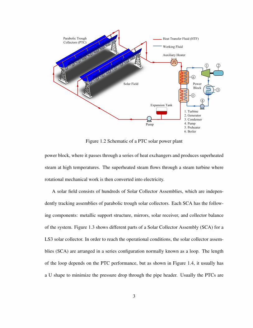
Figure 1.2 Schematic of a PTC solar power plant

power block, where it passes through a series of heat exchangers and produces superheated

steam at high temperatures. The superheated steam flows through a steam turbine where

rotational mechanical work is then converted into electricity.

A solar field consists of hundreds of Solar Collector Assemblies, which are indepen-

dently tracking assemblies of parabolic trough solar collectors. Each SCA has the follow-

ing components: metallic support structure, mirrors, solar receiver, and collector balance

of the system. Figure 1.3 shows different parts of a Solar Collector Assembly (SCA) for a

LS3 solar collector. In order to reach the operational conditions, the solar collector assem-

blies (SCA) are arranged in a series configuration normally known as a loop. The length

of the loop depends on the PTC performance, but as shown in Figure 1.4, it usually has

a U shape to minimize the pressure drop through the pipe header. Usually the PTCs are

3

LSCA

Reflectors

PylonLocal Control

Central pylon with the hydraulic drive unit

Receiver Tube ReceiverTube

w

Reflectors

MetallicStructure

Hydraulic drive unit

Figure 1.3 Parts of a Solar Collector Assembly (SCA). Adapted from [3]

oriented North-South and tracking the sun from east to west, but this also depends on the

land constraints.

The economic feasibility of PTC solar plants is based on finding the optimum size for a

given electric output. The preliminary analysis is performed by the integration of the com-

plex models and components, which are integrated to simulate real operating conditions.

This dissertation proposes the development of a simple methodology for the initial design

of parabolic trough solar systems based on physical models. The methodology is focused

in obtaining a preliminary optimum design through a simplified methodology based on

correlations obtained from detailed component simulations. This methodology is expected

Solar collector

From Cold Header

To Hot Header

Figure 1.4 Schematic of LS-3 solar collector loop. Adapted from [3]

4

to be great help for engineers for the design and performance analysis of parabolic trough

solar systems.

1.1 Literature Review

One of the first solar power plant simulations was developed by Lippke [5]. A typical

30 MWe SEGS plant was studied using a detailed thermodynamic model. In this model,

correlations for the performance of parabolic trough solar collectors were derived based

on measured data under different conditions; these correlations were used to calculate the

energy obtained from the solar field. The model was used to calculate the gross and net

electricity output under different operating conditions.

A detailed heat transfer analysis and modeling of a parabolic trough solar receiver was

carried out by Forristall [6]. One and two dimensional energy balances were used for short

and long receivers respectively. This model was used to determine the thermal perfor-

mance of parabolic trough collectors under different operating conditions. Jones et al. [7]

accomplished a comprehensive model of the 30 MWe SEGS VI parabolic trough plant in

TRNSYS. This model included solar and power cycle performance without fossil backup.

The model was created to accurately predict the SEGS VI plant behavior and to examine

transient effects such as start up, shutdown, and system response. Likewise, Stuetzle [8, 9]

investigated the thermal performance of SEGS VI parabolic trough plant. The analysis con-

sisted of a dynamic model for the collector and a steady-state model for the power plant.

This simulation examined the linear model predictive control strategy for maintaining the

solar field at a constant outlet temperature, although maximizing of the gross electricity

produced was not pursued. Quaschning [10] presented a methodology for economic opti-

5

mization of solar plant design as a function of the solar irradiance. This model is able to

find the optimal solar field size for any specific project location.

A complex model for a parabolic trough, including a comprehensive economic analy-

sis, was developed by NREL (National Renewable Energy Laboratory) [11]. The parabolic

trough solar technology was modeled using the methodology developed by Stine and Har-

rigan [12]. The model is capable of modeling a Rankine-cycle parabolic trough plant,

with or without thermal storage, and with or without fossil-fuel backup. Another simula-

tion [13] for the solar field based on SEGS VI was modeled in TRNSYS. In this simula-

tion, the Rankine power cycle was separately modeled; the steady-state power cycle per-

formance was regressed in terms of the heat transfer fluid temperature, heat transfer fluid

mass flow rate, and condensing pressure, and implemented in TRNSYS. Both the solar

field and power cycle models were validated with measured temperature and flow rate data

from the SEGS VI plant. A thermal economical model called Solar Advisor Model (SAM)

was developed by NREL and Sandia National Laboratory [14, 15]. This model calculates

costs, finances, and performance of concentrating solar power and also allows examining

the impact of variation in the physical parameters on the costs and overall performance.

A more recent methodology for the economic optimization of the solar area in either

parabolic trough or complex solar plants was carried out by Montes et al. [16]. Ther-

mal performance for different solar power plants was analyzed at nominal and load condi-

tions. Once annual electric energy generation is known, levelized cost of energy (LCOE)

for the solar plant can be calculated, yielding a minimum LCOE value for a certain opti-

mum solar area. Similarly, an analytic model for a solar thermal electric generating system

6

with parabolic trough collectors was done by Rolim et al. [17]. Three fields of different

collectors were considered, the first field with evacuated absorbers, the second with non-

evacuated absorbers and the third with bare absorbers. Mittelman and Epstein [18] pro-

posed a new power block by using a bottoming Kalina cycle. This cycle has the advantage

that electricity can be produced at low solar insolation (300-400 W/m2).

As it was shown before, the parabolic trough solar power plant simulation is the result

of a combination of complex thermal and cost models. In general the optimizations of

these systems require an extensive computational effort and software resources. A simpli-

fied conceptual and numerical methodology for designing of parabolic trough solar energy

systems was proposed by Stine and Harrigan [19]. This method proposed a design chart

called storage sizing graph, which obtains the optimum collector area for certain location.

The storage sizing graphs are an excellent initial tool for preliminary design of solar power

plants, but they include a simplified thermal models and cost analysis.

Based on the motivation of this dissertation, the chapters follow the following outline.

In Chapter 2, a heat transfer analysis of the PTC solar receiver is performed. The new

model includes new convective correlations and a comprehensive radiation analysis. A fit-

ting equation for the heat losses is obtained for two solar collectors: LS2 and LS3. Chapter

3 presents the design of typical power block for PTC solar plants. The power block is then

simulated under partial load conditions and a fitting equation is obtained to calculate the

net cycle power output, condenser heat transfer rate and heat transfer fluid (HTF) return

temperature. Chapter 4 shows the design of the solar piping layout and the calculation of

the pumping power requirements for circulating the HTF in the solar field. Determination

7

of thermal losses in pipes and expansion vessel are also included in this chapter. Chapter 5

presents the integration of all previous components and systems and describes the method-

ology for the initial and optimum design of PTC solar plants. Two distinct sites are used

for the application of the proposed methodology, and evaluation of different condenser sys-

tems is also carried out. Finally, chapter 6 shows the conclusions and recommendations for

further research.

8

Chapter 2

Solar Radiation

Detailed information about solar radiation availability at any location is essential for

the design and economic evaluation of parabolic trough solar power plants. Long term

measured data of solar radiation are available for a large number of locations in the United

States and other parts of the world. For those locations where long term measured data are

not available different physics and satellite models can be used to estimate the solar energy

availability.

Solar energy is in the form of electromagnetic radiation with the wavelengths ranging

from about 0.3 µm (10−6m) to over 3 µm, which correspond to ultraviolet (less than 0.4

µm), visible (0.4 µm and 0.7 µm), and infrared (over 0.7 µm); most of this energy is

concentrated in the visible and the near-infrared wavelength range. The incident solar

radiation, sometimes called insolation, is measured as irradiance, or the energy per unit

time per unit area (kW/m2). The average amount of solar radiation falling on a surface

normal to the rays of the sun outside the atmosphere of the earth, extraterrestrial insolation,

at mean earth-sun distance Do is called the solar constant, Io. Recently, new measurements

have found the value of solar constant to be 1366.1 W/m2 [20].

9

23.45 °

June 21

Dec 21

Sun

Axis of revolution of the earth about the sun

23.45 °N

S

N

S

23.45 °

23.45 °Equator

Equator

Tropic of Capricorn, latitude 23.45 S

Tropic of Cancer, latitude 23.45 N

1.521 x 10¹¹ m1.471 x 10¹¹ m

Figure 2.1 Motion of the earth about the sun. Adapted from [21]

2.1 Solar Angles

The variation in seasonal solar radiation availability at the surface of the earth can be

understood from the geometry of the relative movement of the earth around the sun. The

distance between the earth and the sun changes throughout the year, the minimum being

1.471×1011 m at winter solstice (December 21) and the maximum being 1.521×1011 m

at summer solstice (June 21). The year round average earth sun distance is 1.496× 1011

m. The amount of solar radiation intercepted by the earth, therefore varies throughout the

year, the maximum being on December 21 and the minimum on June 21 (Figure 2.1).

The axis of the earth’s daily rotation around itself is at an angle of 23.45 ° to the axis of

its ecliptic orbital plane around the sun. This tilt is the major cause of the seasonal variation

of the solar radiation available at any location on the earth. The angle between the earth-sun

line (through their center) and the plane through the equator is called the solar declination

angle, δs (Figure 2.2). The declination angle varies between -23.45° on December 21 to

+23.45° on June 21. The solar declination is given by:

10

DecNovOctSepAugJulJunMayAprFebJan

Wintersolstice

Autumnal equinox

Summersolstice

Vernalequinox

Mar

Dec

linat

ion

Ang

le, δ

s (d

egre

es)

-23.45

0.00

23.45

Figure 2.2 Variation of the declination angle, δs, throughout the year

δs = 23.45◦ sin[

360 (284+n)365

](2.1)

where n is the day number with January 1 being n = 1. In general, the declination is

assumed to remain constant during a specific day. The analysis of the sun motion is based

on the Ptolemaic theory, which assumes that the earth is fixed and the sun rotates around

the earth. The Ptolemaic view describes the relative sun motion with a coordinate system

fixed to the earth with its origin at the location of interest.

The position of the sun can be described at any time by two angles, the altitude and

azimuth angle (Figure 2.3). The solar altitude angle, α , is the angle between a line collinear

with the sun rays and the horizontal plane [21]. The solar azimuth angle, as, is the angle

between a due south line and the horizontal projection of the line joining the site to the

sun [21]. The sign convention used for azimuth angle is positive west of south and negative

east of south. The solar zenith angle, z is the angle between the site to sun line and the

vertical at the site location:

z = 90−α (2.2)

11

®

z

as

n (north)

s (south)e (east)

w (west)

Sun

S0

i0

j0

k0

z (zenith)

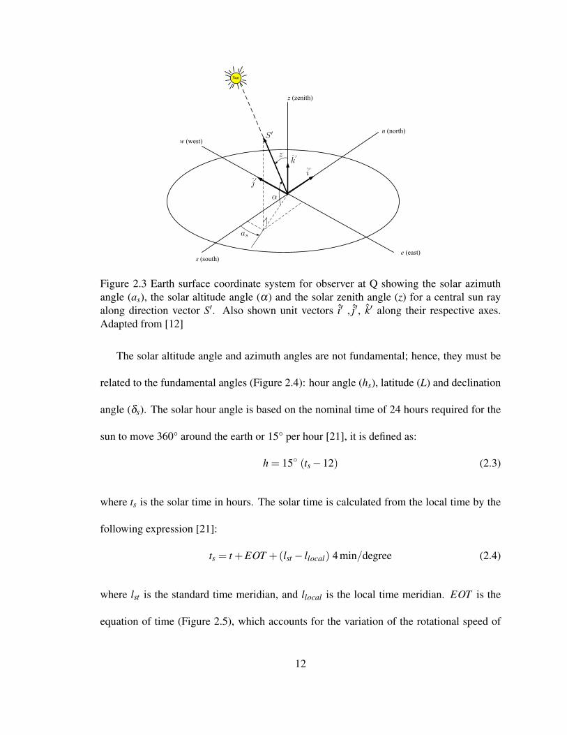
Figure 2.3 Earth surface coordinate system for observer at Q showing the solar azimuthangle (as), the solar altitude angle (α) and the solar zenith angle (z) for a central sun rayalong direction vector S′. Also shown unit vectors i′ , j′, k′ along their respective axes.Adapted from [12]

The solar altitude angle and azimuth angles are not fundamental; hence, they must be

related to the fundamental angles (Figure 2.4): hour angle (hs), latitude (L) and declination

angle (δs). The solar hour angle is based on the nominal time of 24 hours required for the

sun to move 360° around the earth or 15° per hour [21], it is defined as:

h = 15◦ (ts−12) (2.3)

where ts is the solar time in hours. The solar time is calculated from the local time by the

following expression [21]:

ts = t +EOT +(lst− llocal) 4 min/degree (2.4)

where lst is the standard time meridian, and llocal is the local time meridian. EOT is the

equation of time (Figure 2.5), which accounts for the variation of the rotational speed of

12

N

S

Sun Rays

Meridian of observer at Q

Equator

Q

O

L

±s

h

Meridian parallel to sun rays

Declination angle

Figure 2.4 Fundamental sun angles: hour angle h, latitude L and declination δs. Adaptedfrom [12]

the earth. An approximation for calculating the equation of time, EOT ,in minutes is given

by Woolf [22] and is accurate to within about 30 seconds during daylight hours:

EOT = 0.258 cos x−7.416 sin x−3.648 cos 2x−9.228 sin 2x (2.5)

x =360 (n−1)

365.242(2.6)

- Sun slow

+ Sun Fast

DecNovOctSepJul AugMayMarFebJan JunApr

Equa

tion

of T

ime

(min

utes

)

−20

−15

−5

0

5

10

15

20

Figure 2.5 Equation of time EOT

13

The latitude angle L (Figure 2.4) is the angle between the line from the center of the

earth to site and the equatorial plane. The latitude is considered positive north of the equator

and negative south of the equator. Expression for solar altitude and solar azimuth may be

defined in terms of latitude (L), hour angle (h), and declination angle (δs). As it is shown

in Figure 2.3, the unit direction vector S′ pointing toward the sun from the observer Q is

defined as:

S′ = S′i i′ + S′j j′ + S′k k′ (2.7)

where i′ , j′, k′ are unit vectors along n, w, and z axes respectively. The direction cosines

corresponding to n, w, and z axes are S′i, S′j, and S′k, respectively. They can be written in

terms of the solar altitude and azimuth as:

S′i = −cos α cos as

S′j = cos α sin as (2.8)

S′k = sin α

Similarly, a direction vector pointing to the sun can be described at the center of the

earth as shown in Figure 2.6. Using a new set of coordinates, the direction vector S pointing

to the sun may be described in terms of direction cosines Si, S j, and Sk as:

S = Si i + S j j + Sk k (2.9)

Si = −cos δs cos h

S j = cos δs sin h (2.10)

Sk = sin δs

14

±s

e (east)

Sun

S

ij

k

h

Q

m

C (Center of earth)

Equatorial plane

(Polar axis)p

Polaris

Observer meridian

Solar meridian

Figure 2.6 Earth center coordinate system for the sun ray direction vector S defined in termsof hour angle (h), and declination angle (δs). Adapted from [12]

These two sets of coordinates are interrelated by a rotation about e axis (Figure 2.7)

through the complement of the latitude angle (90−L) and the translation along the earth

radius QC. The translation along the earth’s radius is negligible since this is about 1/23525

of the distance from the earth to the sun. Note that the rotation about the e axis is in the

negative sense based on the right-hand rule. In matrix rotation this takes the form:

∣∣∣∣∣∣∣∣∣∣∣∣

S′i

S′j

S′k

∣∣∣∣∣∣∣∣∣∣∣∣=

∣∣∣∣∣∣∣∣∣∣∣∣

sin L 0 cos L

0 1 0

−cos L 0 sin L

∣∣∣∣∣∣∣∣∣∣∣∣·

∣∣∣∣∣∣∣∣∣∣∣∣

Si

S j

Sk

∣∣∣∣∣∣∣∣∣∣∣∣(2.11)

15

±s

e (east)

Sun

S

ij

k

h

Q

m

C (Center of earth)

Equatorial plane

(Polar axis)p

Polaris

Observer Meridian

m

Qz

np

Polaris

C

e axisLi

k

Figure 2.7 Earth surface coordinates after translation from the earth center C to the observerat Q. Adapted from [12]

Solving, it is obtained that:

S′i = Si sin L+Sk cos L

S′j = S j (2.12)

S′k = −Si cos L+Sk sin L

After replacing the corresponding direction cosines, the following set of equations are ob-

tained:

− cos α cos as = −cos δs sin Lcos h + sin δs cos L (2.13a)

cos α sin as = cos δs sin h (2.13b)

sin α = cos δs cos Lcos h + sin δs sin L (2.13c)

Equation (2.13c) is an expression for the solar altitude angle in terms of the observer’s

location (Latitude angle), the hour angle (time) and the sun’s declination (date). Solving

for the solar altitude angle:

α = sin−1 (sin δs sin L+ cos δs cos Lcos h) (2.14)

16

Two expressions for calculating the solar azimuth angle (as) from either Equation

(2.13a) or (2.13b) were obtained. The solar azimuth angle can be in any of the four trigono-

metric quadrants depending on the location, time of day, and the season. Both Equations

(2.13a) or (2.13b) require a test to know the proper quadrant. For Equation (2.13a) the

appropriate procedure for calculating as is:

as = cos−1(

cos δs sin Lcos h − sin δs cos Lcos α

)(2.15)

if h < 0 then as =−|as|

For Equation (2.13b), the procedure is as follows:

as = sin−1(

cos δs sin hcos α

)(2.16)

For L > δs:

if cos h <

(tan δs

tan L

)then |as|> 90

and

as =

−180+ |as| h < 0

180−|as| h≥ 0

(2.17)

if cos h≥(

tan δs

tan L

)then |as| ≤ 90

and

if h < 0 then as =−|as|

17

For L≤ δs the sun remains north of the east-west line (|as|> 90) and the value of as is given

by Equation (2.17). The previous procedure is derived from the path of the sun across the

sky, which can be viewed as a disc displaced from the observer. This geometric perspective

of the sun’s path is helpful to visualize the sun movements and obtain expressions for

testing the sun angles [12].

The sun may be viewed as traveling about a disc of radius R at a constant rate of 15

degrees per hour. As shown in Figure 2.8(a), the center of this disc appears at different

seasonal locations along the polar axis, which passes through the observer at Q and is

inclined to the horizon by the latitude angle. The center of the disc is coincident with the

observer Q at the equinoxes and is displaced from the observer by a distance of R tan δs at

other times of the year. The extremes of this travel are at the solstices. Figure 2.8(b) is a

side view of the sun’s disc looking from the east. In the summer, the sun path disc of radius

R has its center Y displaced above the observer Q. Point X is defined by a perpendicular

from Q. In the n-z plane, the projection of the position S onto the line containing X and Y

will be where the hour angle, h, is. The appropriate test for the sun being in the northern

sky is then:

R cos h < XY (2.18)

The distance XY is:

XY = Rtan δs

tan L(2.19)

then

18

R

To Polaris

N

Summer solstice

Equinoxes

Wintersolstice

Noon

Noon

Noon2:00

4:00

6:00

2:00

1:002:00

3:00

4:00

5:00

6:00

7:008:00 Horizon

L

Q

(a) Solar disc

To Polaris

n (north)

z (zenith)

±s

L

X

Y

R cos h

Arbitrary sun positionS

Horizon surface

NS

W

E

R

R cos h

h

Sun path disc

(b) Side view of the sun’s disc

Figure 2.8 Geometric view of the sun’s path as seen by an observer at Q. Adapted from[12, 21]

19

cos h <tan δs

tan L(2.20)

Sunrise and sunset times can be estimated by finding the hour angle at α = 0, then:

hsr or hss =± cos−1 (− tan L tan δs) (2.21)

2.2 Hourly Solar Radiation Models

The average amount of solar radiation falling on a surface normal to the rays of the sun

outside the atmosphere of the earth (extraterrestrial) at mean earth-sun distance is called

the solar constant, Io. In this simulation the solar constant has a value of 1366.1 W/m2 as

calculated by Gueymard [20]. Figure 2.9 shows the extraterrestrial solar radiation spec-

IR

Air mass 1.5, P 1013.3 mb, Ta 288.2 K, Teo 225.4 KO3 0.34 cm, N2 2.04 E-4 cm, H2O 1.419 cm, RH 45.5% τ a5 0.27, 760 W/m2

Black body curve 5776 K (normalized) 1366.1 W/m2Air mass zero solar spectrum, 1366.1 W/m2

UV

Visible

Spec

tral I

rradi

ance

(W/m

2 μ m

)

0

400

800

1200

1600

2000

2400

Wavelength λ (μ m)0.2 0.8 1.4 2 2.6

Figure 2.9 Extraterrestrial solar radiation spectrum (in vacuum below 280 nm, in airabove 280 nm); also shown are equivalent black body and atmosphere-attenuated spectra(SMARTS2, U.S. Standard Atmosphere USSA, rural aerosol model, Z=48.19° (Air mass1.5)). Adapted from [20, 23]

20

trum, with the solar constant of 1366.1 W/m2, with the equivalent black body (normalized)

curve and the atmosphere attenuated spectrum for air mass of 1.5. The seasonal variation of

extraterrestrial solar radiation at the surface of the earth is well understood from the relative

movement of the earth around the sun. The extraterrestrial radiation varies by the inverse

distance square from the earth to the sun as:

I = Io (Do/D)2 (2.22)

where D is the distance between the sun and the earth, and Do is the yearly mean earth-sun

distance (1.496 × 1011m). The factor (Do/D)2 is calculated as [21]:

(Do/D)2 = 1.00011+0.034221 cos(x)+0.00128 sin(x)

+0.000719 cos (2 x)+0.000077 sin(2 x) (2.23)

x = 360 (n−1)/365◦

Figure 2.10 shows the variation of the factor (Do/D)2 throughout the year. As extraterres-

trial solar radiation, I , passes through the atmosphere, a part of it is reflected back into

DecNovOctSepAugJulJunMayAprMarFebJan

Extra

terre

stria

l rad

iatio

n / S

olar

con

stant

(I/

I o)

0.96

0.98

1

1.02

1.04

Figure 2.10 Variation of (Do/D)2 throughout the year

21

the space, a part is absorbed by the air and water vapor, and some gets scattered by the

molecules of air, water vapor, aerosols and dust particles (Figure 2.11) [21]. The part of

solar radiation that reaches the surface of the earth with essentially no change in direction

is called direct or beam radiation. The scattered diffuse radiation reaching the surface from

the sky is called sky diffuse radiation.

Sun

Extraterrestrial Solar Radiation

Refrected

AbsorbedWater, CO2 Scattered Molecules

dust

DiffuseDirect

Earth

Figure 2.11 Attenuation of solar radiation as it passes through the atmosphere. Adaptedfrom [21]

Determination of the hourly solar radiation received during the average day of each

month is primordial for calculating the solar collector performance throughout the day.

The long term models provide the mean hourly distribution of global radiation over the

average day of each month. Given the long term average daily total and diffuse irradiation

on a horizontal surface, Hh and Dh respectively, it is possible to find the long term hourly

solar radiation: Ih and Id,h. Values of Hh and Dh can be obtained from either ground

measurement data or satellite data [24]. Satellite data provide information about solar

22

radiation and meteorological conditions in locations where ground measurement data are

not available.

For solar radiation calculation, Daily integration approach (Model DI) [25] was used

as the hourly radiation model. Gueymard [25] developed the Daily integration approach

to predict the monthly-average hourly global irradiation by using a large data set of 135

stations with diverse geographic locations (82.58 N to 67.68 S) and climates. Gueymard

compared his proposed model with previous hourly radiation models, Collares-Pereira and

Rabl Model CP&R [26] and Collares-Pereira and Rabl Model modified by Gueymard [27],

and concluded that the daily integration model is the most accurate compared to the other

models.

Total instantaneous solar radiation on a horizontal surface, Ih, is the sum of the beam or

direct radiation, Ib,h, and the sky diffuse radiation Id,h:

Ih = Ib,h + Id,h (2.24)

Referring to Figure 2.12, Ih may be expressed as:

Ih = Ib,N cos z+ Id,h (2.25)

or

Ih = Ib,N sin α + Id,h (2.26)

The hourly beam radiation, Ib,h is obtained from Equation (2.24):

Ib,h = Ih− Id,h (2.27)

23

Sun

Vertical

Beam RadiationIb;N sin ®

Ib;N cos z

®

z

Diffuse RadiationId;h

zIb;N

Ib;h

zA C

B

= Ib;N cos z

Ib;h = Ib;NABAC

= Ib;N sin ®

Figure 2.12 Solar radiation on a horizontal surface. Adapted from [21]

Introducing the hourly to daily ratios rd and rt as:

rd =Id,h

Dh(2.28)

rt =Ih

Hh(2.29)

Then, the beam radiation is:

Ib,h = rt Hh− rd Dh (2.30)

Liu and Jordan [28] showed that rd is well expressed by (Figure 2.13):

rd =π

Tcos h− cos hss

sin hss−hss cos hss(2.31)

The daily-average extraterrestrial irradiation on a horizontal surface, Ho, may be calculated

as a function of the solar constant, Esc, as:

Ho =24π

hss REsc sin ho (2.32)

24

6 1/2 5 1/2

4 1/2

3 1/2

2 1/2

1 1/2

1/2

Time of day (Hours from Solar Noon)

Liu and Jordan (1960)

r d

0.00

0.05

0.10

0.15

0.20

Sunset hour angle hss, in degrees from solar noon60 70 80 90 100 110 120

Figure 2.13 Variation of rd , diffuse conversion factor, with the sunset hour angle for differ-ent times of the day. Adapted from [26, 28]

where hss is the sunset hour angle (+) in radians defined by Equation 2.21. During polar

days and nights, the value of hss is given by:

hss =

0 if − tan L tan δs > 1

π if − tan L tan δs <−1

(2.33)

where ho is the daily average solar elevation outside of the atmosphere, defined by:

ho = q A(hss)/hss (2.34)

and

q = cos L cos δs (2.35)

A(hss) = sin hss−hss cos hss (2.36)

25

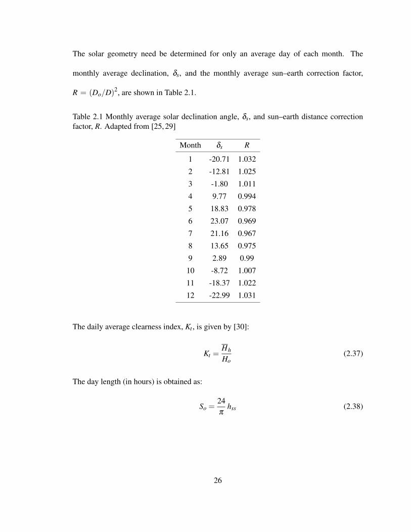
The solar geometry need be determined for only an average day of each month. The

monthly average declination, δs, and the monthly average sun–earth correction factor,

R = (Do/D)2, are shown in Table 2.1.

Table 2.1 Monthly average solar declination angle, δs, and sun–earth distance correctionfactor, R. Adapted from [25, 29]

Month δs R

1 -20.71 1.032

2 -12.81 1.025

3 -1.80 1.011

4 9.77 0.994

5 18.83 0.978

6 23.07 0.969

7 21.16 0.967

8 13.65 0.975

9 2.89 0.99

10 -8.72 1.007

11 -18.37 1.022

12 -22.99 1.031

The daily average clearness index, Kt , is given by [30]:

Kt =Hh

Ho(2.37)

The day length (in hours) is obtained as:

So =24π

hss (2.38)

26

The ratio of the horizontal hourly radiation to the total horizontal daily radiation, rt , is given

by:

rt = rd1+q (a2/a1) A(hss) rd (24/π)

1+q (a2/a1) B(hss)/A(hss)(2.39)

where (a2/a1) represents the atmospheric extinction effect. a1 and a2 were obtained from

a multiple least-squares fit:

a1 = 0.41341Kt +0.61197K2t −0a.01886Kt So +0.00759So (2.40)

a2 = Max(0.054, 0.28116+2.2475Kt−1.7611K2

t −1.84535 sin ho

+1.681 sin3 ho)

(2.41)

and B(hss) is defined as:

B(hss) = ωs(0.5+ cos2 hss

)−0.75 sin (2hss) (2.42)

For a parabolic trough solar collector, only the beam radiation on the aperture area, Ib,c,

is needed [21]. The beam radiation, Ib,c, is calculated as:

Ib,c =(rt Hh− rd Dh

) cos isin α

(2.43)

where i is the angle of incidence, which depends on the tracking mode and the position

of the sun. In order to optimize the PTC performance, two different tracking mode are

used (Figure 2.14): North-South (East-West axis tracking) and East-West (North-South

axis tracking). The next section shows how to calculate cos i for single axis tracking.

27

n (north)

s (south)e (east)

w (west)

Tracking axis

Aperturearea

(a) East-West (North-South axis tracking)

n (north)

s (south) e (east)

w (west) Tracking axis

Aperturearea

(b) North-South (East-West axis tracking)

Figure 2.14 Tracking mode for PTCs

2.3 Single Axis Tracking

As it was mentioned before, PTCs are designed to operate with tracking about only one

axis. A tracking drive system rotates the collector about an axis of rotation until the sun

central ray and the aperture normal area are coplanar. Figure 2.15 shows how the rotation

of a collector aperture about a tracking axis r. The tracking angle, ρ , brings the central ray

unit vector S into the plane formed by the aperture normal and the tracking axis. To write

expressions for i and ρ in terms of the collector orientation and solar angles, it is necessary

to transform the initial coordinates , x′, y′, z′ (Figure 2.3) to a new coordinate system that

has the tracking axis as one of its three orthogonal axes. The other two axes are oriented

Sun

S

N

i

(aperture normal)

½ (tracking angle)

r(tracking axis)

Figure 2.15 A single-axis tracking aperture. Adapted from [12]

28

½(tracking angle)

r(tracking axis)

½

S

N

Rotation path of aperture normal N

u

Su

Sb

Sr

Sun

(+)

b

i

Figure 2.16 Single-axis tracking system coordinate. Adapted from [12]

such as that one axis is parallel to the surface of the earth. Figure 2.16 shows the new

coordinate system, where r is the tracking axis, b is the axis that always remains parallel to

the earth surface and u is the third orthogonal axis. Note that the aperture normal N rotates

in the u− b plane. Both i and ρ can be defined in terms of the direction cosines of the

central ray unit vector S along the u, b, and r axes. The tracking angle is defined by1:

tan ρ =−Su

Sb(2.44)

and the cosine of incidence angle, i, is given by:

cos i =√

S2b +S2

u (2.45)

or

cos i =√

1−S2r (2.46)

1The sign minus is based on the right hand rule

29

2.3.1 Horizontal Tracking Axis

To describe this category, we must rotate the u, b, and r coordinates by an angle γ from

the z, w, and n coordinates that were previously used to describe the sun ray unit vector

(Figure 2.16). Since the axis tracking remains parallel to the earth surface, the rotation

takes place about the z axis as shown in Figure 2.17. The direction cosines of S (new

coordinate system) are calculated as2:

∣∣∣∣∣∣∣∣∣∣∣∣

Sr

Sb

Su

∣∣∣∣∣∣∣∣∣∣∣∣=

∣∣∣∣∣∣∣∣∣∣∣∣

cos γ −sin γ 0

sin γ cos γ 0

0 0 1

∣∣∣∣∣∣∣∣∣∣∣∣·

∣∣∣∣∣∣∣∣∣∣∣∣

S′i

S′ j

S′k

∣∣∣∣∣∣∣∣∣∣∣∣(2.47)

b

r

°

n (north)

e (east)

(tracking axis)

(horizontal axis)

w (west)z, u

Figure 2.17 Rotation of u, b, and r from z, w, and n coordinates about the z axis. Adaptedfrom [12]

Substituting into Equation (2.44), it is obtained that the tracking angle is:

tan ρ =sin (γ−as)

tan α(2.48)

2Note that this rotation is in the negative direction based on the right-hand rule

30

The angle of incidence for a single axis, horizontal tracking collector is:

cos θi =√

1− cos2 α cos2 (γ−as) (2.49)

When the tracking axis is oriented in the north-south direction (γ = 0), the equations above

reduce to:

tan ρ =−sin as

tan α(2.50)

and

cos i =√

1− cos2 α cos2 as (2.51)

When the tracking axis is oriented in the east-west direction (γ = 90), the Equations (2.48)

and (2.49) become:

tan ρ =cos as

tan α(2.52)

and

cos i =√

1− cos2 α sin2 as (2.53)

2.4 Results

For the design of parabolic trough solar plants, two locations were selected: Tampa and

Daggett. The latitude and longitude of these locations are specified in Table 2.2.

Table 2.2 Locations used for the design of parabolic trough solar plants

Location Latitude Longitude

Tampa, Fl 27.97◦ -82.53◦

Daggett, CA 34.85◦ -116.80◦

31

The results obtained for solar radiation calculations, using two different radiation data

sources: TMY3 [32] and Surface meteorology and Solar Energy (NASA-SSE) [24], are

shown in Figures 2.18 and 2.20. Figure 2.18 shows the comparison of the three hourly solar

radiation models: CP&R, CP&RG and DI model. The three model show minor differences

for the monthly average beam radiation. This agrees with the results obtained by Gueymard

[25], who found that DI model showed better performance at high latitudes than the other

models but at low latitudes the differences were small. Figures 2.19 and 2.20 show the

effect of the tracking axis on the beam radiation. As it was expected, for both locations,

the North-South axis tracking presents better performance during most of the year. For that

reason most of the PTCs are oriented with their tracking axis in the North-South direction.

Figure 2.21 shows the annual total radiation obtained for each tracking axis, again the new

results are more favorable for the North-South axis tracking, therefore this configuration

will be adopted for the calculation of solar radiation in this dissertation.

CP&R (Collares-Pereira and Rabl, 1979)CP&RG (Gueymard, 1986)DI Model (Gueymard, 2000)

Mon

thly

Ave

rage

Bea

m R

adia

tion

(kW

h/m

2 -day

)

2

3

4

5

6

7

8

9

10

Jan Feb Mar Apr May Jun Jul Aug Sep Oct Nov Dec

(a) Tampa

CP&R (Collares-Pereira and Rabl, 1979)CP&RG (Gueymard, 1986)DI Model (Gueymard, 2000)

Mon

thly

Ave

rage

Bea

m R

adia

tion

(kW

h/m

2 -day

)

2

3

4

5

6

7

8

9

10

11

Jan Feb Mar Apr May Jun Jul Aug Sep Oct Nov Dec

(b) Daggett

Figure 2.18 Comparison of different hourly radiation models. Radiation data source:NASA-SSE [24], hourly radiation model: CP&R [31], CP&RG [27] and DI model [25]

32

NASA-SSETMY3

Mon

thly

Ave

rage

Bea

m R

adia

tion

(kW

h/m

2 -day

)

2

4

6

8

10

Jan Feb Mar Apr May Jun Jul Aug Sep Oct Nov Dec

(a) North-South Axis Tracking

NASA-SSETMY3

Mon

thly

Ave

rage

Bea

m R

adia

tion

(kW

h/m

2 -day

)

2

4

6

8

10

Jan Feb Mar Apr May Jun Jul Aug Sep Oct Nov Dec

(b) East-West Axis Tracking

Figure 2.19 Effect of tracking axis and data radiation source on the monthly average beamradiation for Tampa. Radiation data source: NASA-SSE [24] and TMY3 [32], hourlyradiation model: DI model [25]

NASA-SSETMY3

Mon

thly

Ave

rage

Bea

m R

adia

tion

(kW

h/m

2 -day

)

2

4

6

8

10

12

Jan Feb Mar Apr May Jun Jul Aug Sep Oct Nov Dec

(a) North-South Axis Tracking

NASA-SSETMY3

Mon

thly

Ave

rage

Bea

m R

adia

tion

(kW

h/m

2 -day

)

2

4

6

8

10

12

Jan Feb Mar Apr May Jun Jul Aug Sep Oct Nov Dec

(b) East-West Axis Tracking

Figure 2.20 Effect of tracking axis and data radiation source on the monthly average beamradiation for Daggett. Radiation data source: NASA-SSE [24] and TMY3 [32], hourlyradiation model: DI model [25]

The DI model, along with radiation data from NASA-SSE were used to map the direct

and beam radiation. The maps were plotted using the Matplotlib Basemap Toolkit [33]

in Python 2.6 [34]. Given the resolution of the radiation data obtained from NASA-SSE

33

Tampa (TMY3)Tampa (NASA-SSE)Daggett (TMY3)Daggett (NASA-SSE)

Ann

ual T

otal

Rad

iatio

n (k

Wh/

m2 -y

eary

)

0

500

1000

1500

2000

2500

3000

North-South Axis East-West Axis

Figure 2.21 Comparison of the annual total beam radiation for different tracking axis andsolar radiation data source. Radiation data source: NASA-SSE [24] and TMY3 [32], loca-tion: Tampa and Daggett, hourly radiation model: DI model [25]

25�N

30�N

35�N

40�N

45�N

125�W 120�W 115�W 110�W 105�W 100�W 95�W 90�W 85�W 80�W 75�W

Annual Average (kWh/m2 - day)

2

3

4

5

6

7

8

9

Figure 2.22 Solar direct beam radiation map for USA. Radiation data source: NASA-SSE[24], hourly radiation model: DI model [25]

34

25�N

30�N

35�N

40�N

45�N

125�W 120�W 115�W 110�W 105�W 100�W 95�W 90�W 85�W 80�W 75�W

Annual Average (kWh/m2 - day)

2

3

4

5

6

7

8

9

Figure 2.23 Solar beam radiation map (North-South axis tracking) for USA. Radiation datasource: NASA-SSE [24], hourly radiation model: DI model [25]

24�N

26�N

28�N

30�N

32�N

88�W 86�W 84�W 82�W 80�W 78�W

Annual Average (kWh/m2 - day)

2

3

4

5

6

7

8

9

(a) Direct Beam Radiation

24�N

26�N

28�N

30�N

32�N

88�W 86�W 84�W 82�W 80�W 78�W

Annual Average (kWh/m2 - day)

2

3

4

5

6

7

8

9

(b) Beam Radiation for North-South AxisTracking

Figure 2.24 Solar radiation map for Florida. Radiation data source: NASA-SSE [24],hourly radiation model: DI model [25]

35

(1◦×1◦), it was necessary to use a bilinear interpolation [33] for obtaining data at higher

resolution. Figures 2.22 and 2.23 show the maps obtained for the North-South axis track-

ing beam radiation for USA, while Figure 2.24 shows the results for Florida. The results

showed that in general Florida has acceptable levels of beam radiation. Lower levels of ra-

diation increase the cost of the Concentrated Solar Power (CSP) plants and therefore their

economic viability.

2.5 Solar Shading

The solar shading on PTC (Parabolic trough collector) was initially solved using only

one concentrating collector (Figure 2.25).

Figure 2.25 Solar shading problem with only one concentrating collector

For a simple object, its shadow is defined by (Figure 2.26):

LSH =L

tan α(2.54)

where L is the length of the object, and LSH is the length of the object’s shadow. For a PTC,

the shading was calculated with the projected area (rectangular projected section) and each

36

®

as

n (north)

s (south)e (east)

w (west)

Sun

S

L

Lsh

Figure 2.26 Geometry used to calculate the shadow of an object

shadow projection was assumed to be parallel. Figure 2.27 shows the geometry used to

solve the problem. Using the previous expression, it is obtained:

LS1 =d1−

a2

sin ζ

tan α(2.55)

a

fa

fb

³

d1 +a

2sin ³

d1

d1 ¡

a

2sin ³

b

as

a cos ³as as

Ls1

Ls1

Ls2

Ls2

b

Figure 2.27 Simplified geometry used for one concentrating collector

37

LS2 =d1 +

a2

sin ζ

tan α(2.56)

with

d1 = fa + fb cos ζ

As seen in Figure 2.27, the shading area is given by:

ASH = b ·a[

a cos ζ +sin ζ sin as

tan α

](2.57)

It is also important to obtain an expression for σ (Figure 2.28):

K = a[

cos2ζ +

sin2ζ

tan2 α+

sin 2ζ

tan αsin as

]1/2

(2.58)

Ls1 Ls2

a cos ³as as

¾

Ls2 ¡ Ls1

K

Figure 2.28 Geometry used in a solar shading problem with only one concentrating collec-tor

Using sine law:

sin σ =aK

sin ζ

tan αcos as (2.59)

38

The next expression for σ is obtained:

σ = sin−1

sin ζ cos as

tan α

(cos2 ζ +

sin2ζ

tan2 α+

sin 2ζ

tan αsin as

)1/2

(2.60)

After solving for the shadow of one concentrating collector, the problem with two or

more concentrating collector was then solved. Figure 2.29 shows the geometry used for

this problem. Two variables, b′ and xs, were found. Referring to Figure 2.29, in order to

calculate xs, it is necessary to obtain θ first . The angle θ (Figure 2.30(a)) is given by:

tan θ = tan ζ cos σ (2.61)

xs is obtained from the following expression:

xs =

a sin ζ −(

d−a cos ζ

cos σ

)tan α

cos θ tan α + sin θ(2.62)

The second collector is not shaded when:

asin ζ ≤(

d−a cos ζ

cos σ

)tan α (2.63)

or

tan α ≥ tan αcr (2.64)

αcr is defined as:

tan αcr =sin ζ cos σ

d/a− cos ζ

39

as

as

Ls1Ls2

Ls1Ls2

d

d ¡ a cos ³

b

b0

xs

1 2 3

A

A

d1 +a

2sin ³

d¡ a cos ³

cos ¾

d1 ¡

a

2sin ³

®

1

2

3xs

Figure 2.29 Solar shading problem with two concentrating collectors

³

¾

(a)

³

¾ 0

¾

(b)

Figure 2.30 Geometry used to calculate θ and σ ′

40

Because 0≤ α ≤ 90o, the last expression can be rewritten as:

α ≥ αcr (2.65)

In order to calculate the shading area, it is necessary to calculate σ ′ (Figure 2.30(b)):

tan σ′ = tan σ cos ζ (2.66)

Now, it is necessary to define some conditions based on points P1 and P2 (Figure 2.31).

Point P1 is defined by:

P1 = (x1,y1) (2.67)

x1 = Ls2 sin as +a2

cos ζ (2.68)

y1 = Ls2 cos as (2.69)

Figure 2.31 Interception of the solar shading with the projected area of the parabolic trough

The equation of a straight line is given by:

y− y1 = tan σ (x− x1) (2.70)

41

Point P2 is defined as follows:

P2 = (x2,y2) (2.71)

x2 = d− a2

cos ζ (2.72)

y2 = y1 +m (x2− x1) (2.73)

c = y2 (2.74)

where x2− x1 is given by:

x2− x1 = d−a cos ζ −(

d1 +a2

sin ζ

) sin as

tan α

then

y2 =(

d1 +a2

sin ζ

) cos as

tan α+ tan σ

[d−a cos ζ −

(d1 +

a2

sin ζ

) sin as

tan α

](2.75)

There is no shadow when:

y2 ≥ b

which is equivalent to:

y′2 ≥ R

with

y′2 =

y2

aand R =

ba

42

a

b

a0

b0

(1) (2)

Figure 2.32 Different configurations for the solar shading area

When there is shading, as seen in Figure 2.32, different configurations can be observed.

For case (1):

x′s cos σ

′ < 1 (2.76)

and x′s sin σ ′+ c′ > R Case (a)

x′s sin σ ′+ c′ < R Case (b)

(2.77)

x′s =

xs

a

For case (2):

x′s cos σ

′ > 1 (2.78)

and x′s sin σ ′+ c′ > R Case (a)

x′s sin σ ′+ c′ < R Case (b)

(2.79)

43

For cases 1-a and 2-a’, the shading area (Figure 2.33) is given by:

Ash =(b− c)2

2 tan σ ′(2.80)

b

c b ¡ c

¾0

Figure 2.33 Shading area for configuration 1-a and 2-a’

The expression for c (Figure 2.31) was previously obtained as:

c =(

d1 +a2

sin ζ

) cos as

tan α+ tan σ

[d−a cos ζ −

(d1 +

a2

sin ζ

) sin as

tan α

](2.81)

The fraction of shading area is:

SH =Ash

a b=

(b− c)2

2ab tan σ ′(2.82)

Manipulating the last expression:

SH =(R− c′)2

2R tan σ ′(2.83)

with

R =ba

and c′ =ca

For case 1-b, the shading area (Figure 2.34) is given by:

44

Ash =(

b− c− xs

2sin σ

′)

xs cos σ′ (2.84)

b

b0

c

¾0

xs

Figure 2.34 Shading area for configuration 1-b

The fraction of shading area is:

SH =Ash

a b=

(R− c′− x′s

2sin σ

′)

x′sR

cos σ′ (2.85)

x′s =xs

a

For case 2-b’, the shading area (Figure 2.35) is calculated as:

Ash =(

b− c− a2

tan σ′)

a (2.86)

In this case xs is given by the next expression:

xs cos σ′ = a (2.87)

The fraction of shading area is:

SH =Ash

a b=

1R

(R− c′− 1

2tan σ

′)

(2.88)

45

b

c

¾0

b0

Figure 2.35 Shading area for configuration 2-b’

The shading factor is defined by:

ϕSH = 1−SH (2.89)

The procedure for solar shading calculations is shown in Figure 2.36. In order to vali-

date the shading model, it was compared with the model developed by Stuetzle [8] which

assumes that the shadow covers the entire length of the PTC. Table 2.3 shows the input

parameters used for the simulation of the solar shading.

Table 2.3 Input parameters for solar shading simulation

Dimension Value Reference

a 5 m [4]b 400 m [13]d 15 m [13]

Focal Length ( f ) 1.49 m [4]fa a/2 [12]fb a2/(16 f ) [12]

The simulation was carried out by June 21 and December 21 at SEGS VI location

(latitude 37.21◦N and longitude 117.022◦W), the results are shown in Figure 2.37. The

results obtained show that the model developed by Stuetzle is more conservative, although

46

Day number Latitude angle L

Time (hr)

Tracking Angle a

Calculate Solar Angle h

Calculate Solar Declination

Calculate Solar Altitude

Angle a

Solar Azimuth angle aa

Calculate Angle a

Calculate Angle θ

Calculate Angle σ’

Calculate y2

Yes

No

Calculate x’Calculate c’

Calculate SHCase b

Calculate α cr

Yes

YesNo

Yes No

No

Calculate SHCase a

Figure 2.36 Logic flow for calculation of solar shading

47

there are small differences between the models owing to the dimensions of the PTC. For

smaller systems, like small collectors for heating and electricity production, the proposed

model seems to be more appropriate.

December

June

Proposed modelStuetzle (2002)

Shad

ing

Fact

or ψ

SH

0

0.2

0.4

0.6

0.8

1

1.2

Solar time (hr)4 6 8 10 12 14 16 18 20

(a)

JuneDecember

Shad

ing

Fact

or ψ

SH, P

ropo

sed

Mod

el0

0.2

0.4

0.6

0.8

1

Shading Factor ψSH, Stuetzle (2002)0 0.1 0.2 0.3 0.4 0.5 0.6 0.7 0.8 0.9 1

(b)

Figure 2.37 Comparison between the proposed shading model and the model developed byStuetzle [8]. Input parameters are given in Table 2.3

2.6 Conclusions

DI model was selected as the hourly radiation model. The inputs for this model can

be measured data or satellite data, which gives certain flexibility to those locations where

measured radiation data are not available. The results show that North-South axis tracking

is the best tracking configuration for the locations analyzed: Tampa and Daggett.

The solar radiation maps obtained can be an aid to find preliminary locations around the

world where optimum levels of radiation are present, although it is important to emphasize

that solar radiation is only one of the criteria to find optimum locations for Concentrated

Solar Power plants (CSP).

48

A solar shading model was developed; the results showed that the proposed model is

suitable for any PTC dimensions.

49

Chapter 3

Heat Transfer Analysis of Parabolic Trough Solar Receiver

3.1 Introduction

Parabolic trough power plants currently represent the most mature technology for solar

thermal power production. A parabolic trough solar collector (PTC) takes the radiant en-

ergy from the sun and converts it to useful thermal energy in the heat transfer fluid (HTF)

that circulates through the solar field. Once the geometry and thermal properties are de-

fined, the thermal performance and energy gained by the HTF can be calculated under

different configurations and meteorological conditions. PTCs are typically operated at up

to temperatures of 400 ◦C and synthetic oil is commonly used as HTF. The heat transfer

analysis of these collectors is important for the calculation of thermal losses and sizing of

the solar power plant during preliminary design and also permits to evaluate the effects

of collector degradation, and HTF flow rate control strategies on the overall plant perfor-

mance [13]. Given the importance of the heat transfer analysis in PTCs, since the 1970s

numerous models have been proposed.

Edenburn [35] predicted the efficiency of a PTC by using an analytical heat trans-

fer model for evacuated and non evacuated cases. The results showed good agreement

with measured data obtained from Sandia National Laboratories (SNL) collector test fa-

cility [36]. Ratzel et al. [37] carried out both analytical and numerical study of the heat

50

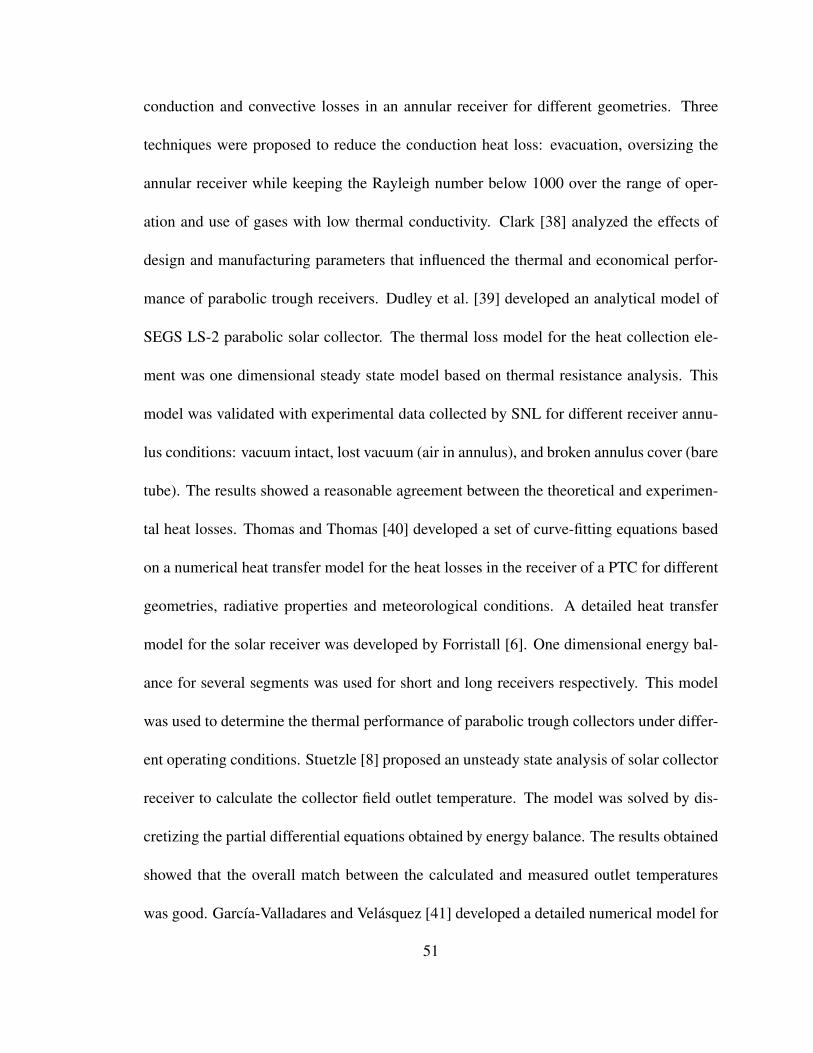
conduction and convective losses in an annular receiver for different geometries. Three

techniques were proposed to reduce the conduction heat loss: evacuation, oversizing the

annular receiver while keeping the Rayleigh number below 1000 over the range of oper-

ation and use of gases with low thermal conductivity. Clark [38] analyzed the effects of

design and manufacturing parameters that influenced the thermal and economical perfor-

mance of parabolic trough receivers. Dudley et al. [39] developed an analytical model of

SEGS LS-2 parabolic solar collector. The thermal loss model for the heat collection ele-

ment was one dimensional steady state model based on thermal resistance analysis. This

model was validated with experimental data collected by SNL for different receiver annu-

lus conditions: vacuum intact, lost vacuum (air in annulus), and broken annulus cover (bare

tube). The results showed a reasonable agreement between the theoretical and experimen-

tal heat losses. Thomas and Thomas [40] developed a set of curve-fitting equations based

on a numerical heat transfer model for the heat losses in the receiver of a PTC for different

geometries, radiative properties and meteorological conditions. A detailed heat transfer

model for the solar receiver was developed by Forristall [6]. One dimensional energy bal-

ance for several segments was used for short and long receivers respectively. This model

was used to determine the thermal performance of parabolic trough collectors under differ-

ent operating conditions. Stuetzle [8] proposed an unsteady state analysis of solar collector

receiver to calculate the collector field outlet temperature. The model was solved by dis-

cretizing the partial differential equations obtained by energy balance. The results obtained

showed that the overall match between the calculated and measured outlet temperatures

was good. García-Valladares and Velásquez [41] developed a detailed numerical model for

51

a single pass solar receiver and validated it. Then they extended the model to a double

pass receiver. Their results showed that the proposed configuration enhances the thermal

efficiency of the solar collector compared with the single pass. Recently, three dimensional

heat transfer analysis of PTCs was performed by combining the Monte Carlo Ray Trace

Method (MCRT) and CFD analysis [42–44]. The results indicated that the flange (support

bracket) and bellow under non-vacuum conditions bring a high conductive heat loss.

In the middle 90s, Cohen and Kerney [45] proposed the use of direct steam generation

(DSG) collector as a future development of the Solar Electric Generating Station (SEGS)

in order to eliminate the costly synthetic oil, intermediate heat transport piping loop and

the heat exchanger between the solar field and the power block. Heidemann et al. [46]

formulated a two dimensional heat transfer model for calculating the absorber wall tem-

perature of a DSG collector under steady and unsteady conditions. The numerical solution

showed that a sudden drop of irradiation induces a very high temperature gradient inside

the absorber tube in a short period of time. Odeh et al. [47] carried out a model for heat

loss of a DSG collector in terms of wall temperature rather than working fluid tempera-

ture. The results were compared with the Sandia test data and the results showed that the

model underestimates the measured loss. This underestimation was attributed to omission

of heat loss from the receiver tube vacuum bellows. Odeh et al. [48] studied the thermal

performance of parabolic trough solar collector used as direct steam generator for different

solar radiation levels and geometric configurations. This heat transfer model showed better

agreement with the in focus test results than the polynomial curve fit equation obtained

by Dudley et al. [39]. The thermal losses calculated for water were based on the receiver

52

wall temperature and the results showed that thermal losses calculated for steam as the heat

transfer fluid were lower than those obtained for synthetic oil.

In this chapter a detailed one dimensional heat transfer analysis of a PTC is presented.

The existing models published previously assume that there is no thermal interaction be-

tween the neighboring surfaces (absorber-envelope, and envelope-envelope) for thermal

radiation losses. Although this assumptions simplifies the analysis, it underestimates the

radiation losses at high absorber temperatures. To account for the thermal interaction be-

tween adjacent surfaces, a comprehensive radiative analysis was implemented in our study

for the heat losses in the absorber and the glass envelope. A review of the correlations for

convective heat transfer losses was performed as well and new correlations were used in

this model. The receiver and envelope were divided into several segments, and mass and

energy balance were carried out in each control volume. The partial differential equations

were discretized by using the finite difference method and the set of nonlinear algebraic

equations were solved simultaneously. In order to validate the proposed numerical model,

it was compared with the experimental data obtained from Sandia National Laboratories

(SNL), Dudley et al. [39], and other heat transfer models [6, 41] as well.

3.2 Solar Receiver Model

The heat collection element (HCE) consists of an absorber surrounded by a glass en-

velope (Figure 3.1). The absorber is typically stainless steel tube with a selective absorber

surface which provides the required optical and radiative properties. Selective surfaces

combine a high absorptance for solar radiation with low emittance for the temperature

range in which the surface emits radiation. This combination of surface characteristics is

53

Expansion bellows Glass EnvelopeAbsorber tube with

selective coatingVacuum between envelope and absorber

f,i f,i+1f,i-1

a,i a,i+1a,i-1

e,i e,i+1e,i-1

Control volume

z

r

Absorber (a)

Envelope (e)

Heat Transfer Fluid (f)

Δz

Figure 3.1 Parts of a heat collection element (HCE) and control volume used for the heattransfer analysis. Adapted from [49]

possible because 98 percent of the energy in incoming solar radiation is contained within

wavelengths below 3 µm [21]. The glass envelope is an anti reflective evacuated glass tube

which protects the absorber from degradation and reduces the heat losses. The vacuum

enclosure is used primarily to reduce heat losses at high operating temperatures and to pro-

tect the solar-selective absorber surface from oxidation. The HCE uses conventional glass

to metal seals and metal bellows at either end to achieve the necessary vacuum enclosure

and for thermal expansion difference between the steel tubing and the glass envelope [4].

The bellows also allow the absorber to extend beyond the glass envelope so that the Heat

54

Collection Elements can form a continuous receiver. The space between bellows provides

a place to attach the HCE support brackets [6]. Chemical getters are placed in the annulus

to absorb hydrogen, which comes from the HTF and decreases the PTC performance.

The heat transfer model is based on an energy balance between the heat transfer fluid

and the surroundings. Figure 3.2 shows the heat transfer in a cross section at the solar

collector and the thermal resistance model used in the heat transfer analysis.

_Qa¡f;conv

_Qcond¡bracket

_Qa¡abs

_Qa¡e;conv _Qa¡e;rad

_Qe¡abs

_Qe¡sa;conv

_Qe¡s;rad

(a) Heat transfer

f a

ConvectionConvection

Radiation

Conduction (Bracket)

e sRadiation

Convection sa

sa

_Qa¡abs_Qe¡abs

(b) Thermal circuit

Figure 3.2 Heat transfer and thermal resistance model in a cross section at the heat collec-tion element (HCE). Adapted from [6, 39]

55

The solar energy reflected by the mirrors is absorbed by the glass envelope Qe−abs and

the absorber surface Qa−abs. A part of the energy absorbed in the absorber is transferred to

the HTF by forced convection Qa− f ,conv, remaining energy is transferred back to the glass

envelope by radiation Qa−e,rad and natural convection Qa−e,conv and lost through the sup-

port brackets by conduction Qcond,bracket as well. The heat loss coming from the absorber

(radiation and natural convection) passes through the glass envelope by conduction and

along with the energy absorbed by the glass envelope Qe−abs is lost to the environment by

convection Qe−sa,conv and to sky by radiation Qe−s,rad [6]. In this heat transfer model the

absorbed radiation was assumed as a heat flux term. In most of the surfaces the thickness

of the surface layer over which absorption is taking place is very small compared with the

overall dimensions, therefore the error associated with this assumption is very low [50,51].

In order to obtain the partial differential equations that govern the heat transfer phenom-

ena, an energy balance was applied over a section of the solar receiver (Figure 3.1). The

equations obtained for each component are showed below.

3.2.1 Heat Transfer from Absorber to Heat Transfer Fluid

Referring to the control volume in Figure 3.3, a uniform temperature and heat flux

distribution around the receiver is assumed. After applying the energy balance on this

control volume, assuming unsteady state and incompressible fluid with [52], h≈Cp T , the

following partial differential equation (PDE) is obtained:

Ai,a ρ f Cp, f∂Tf

∂ t=−m f

∂

∂ z

(Cp, f Tf +

V 2f

2

)+ Q

′a− f ,conv (3.1)

56

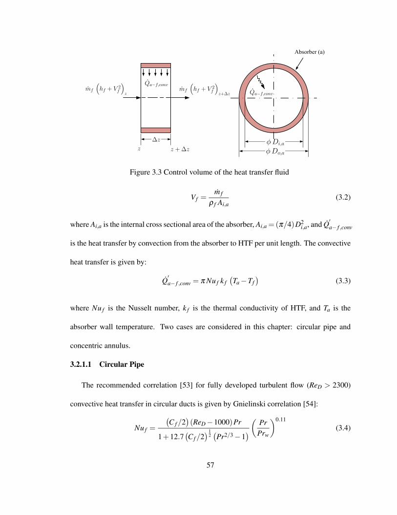
_mf

³hf + V 2

f

´z

_mf

³hf + V 2

f

´z+¢z

z + ¢zz

_Qa¡f;conv

_Qa¡f;conv

¢z Á Di;a

Á Do;a

Absorber (a)

Figure 3.3 Control volume of the heat transfer fluid

Vf =m f

ρ f Ai,a(3.2)

where Ai,a is the internal cross sectional area of the absorber, Ai,a =(π/4)D2i,a, and Q

′a− f ,conv

is the heat transfer by convection from the absorber to HTF per unit length. The convective

heat transfer is given by:

Q′a− f ,conv = π Nu f k f

(Ta−Tf

)(3.3)

where Nu f is the Nusselt number, k f is the thermal conductivity of HTF, and Ta is the

absorber wall temperature. Two cases are considered in this chapter: circular pipe and

concentric annulus.

3.2.1.1 Circular Pipe

The recommended correlation [53] for fully developed turbulent flow (ReD > 2300)

convective heat transfer in circular ducts is given by Gnielinski correlation [54]:

Nu f =

(C f /2

)(ReD−1000)Pr

1+12.7(C f /2

) 12(Pr2/3−1

) ( PrPrw

)0.11

(3.4)

57

ReD =Vf Di,a

ν f

where C f is the friction coefficient (Fanning friction factor), ReD is the Reynolds number

based on the absorber inner pipe diameter, Pr is the Prandtl number, and ν f is the kinematic

viscosity of HTF. This correlation is valid for 2300≤ ReD ≤ 5× 106 and 0.5≤ Pr≤ 2000.

The thermal properties should be evaluated at the bulk mean heat transfer fluid temperature,

except Prw which is evaluated at the absorber wall temperature. The friction coefficient is

calculated from the Filonenko correlation [53] for isothermal flows in smooth tubes:

C f = (1.58LnReD−3.28)−2 104 ≤ ReD ≤ 107 (3.5)

The convection heat transfer coefficient for rough tubes can be calculated approxi-

mately by using the friction coefficient determined from the Colebrook and White equa-

tion [53]:

1√C f

= 3.48−1.7372Ln

(2 ε

Di,a+

9.35ReD

√C f

)5≤ Reε ≤ 70 (3.6)

with

Reε =Vf ε

ν f(3.7)

The best explicit correlation for practical friction coefficient computations in a rough

circular duct is given by Chen [53]:

1√C f

= 3.48−1.7372Ln(

2 ε

Di,a− 16.2426

ReDLnA2

)(3.8)

A2 =(2 ε/Di,a)

1.1098

6.0983+

(7.149ReD

)0.8981

58

for 4000 ≤ ReD ≤ 108 and 2 × 10−8 ≤ 2 ε/Di,a ≤ 0.1. For the transition flow

2100 ≤ ReD ≤ 4000 the formula developed by Bhatti and Shah can be used to calculate

the friction coefficient [55]:

C f = 0.0054+2.3 × 10−8

Re−3/2D

(3.9)

Since entry lengths for turbulent flow are typically short 10 ≤ z/D ≤ 60 , it is often

reasonable to assume that the average Nusselt number for the entire tube is equal to the

value associated with the thermally fully developed turbulent flow [56]. However, for short

tubes the mean Nusselt number for thermally developing flow can be calculated using Al-

Arabi’s correlation [55]:

Nu f ,m

Nu f ,∞= 1+

Cz/D

(3.10)

where Nu∞ stands for the fully developed Nusselt number and:

C =(z/D)0.1

Pr1/6

(0.68+

3000Re0.81

D

)(3.11)

For laminar flow, (ReD ≤ 2300), the Nusselt number on walls with uniform temperature

is given by:

Nu f = 3.66 (3.12)

For a circular tube subjected to constant surface temperature, the average Nusselt num-

ber for the thermal entrance region can be determined from Hausen’s correlation [55]:

Nu f = 3.66+0.0668

z∗1/3(0.04+ z∗2/3

) (3.13)

59

where z∗ = (z/D)/(ReD Pr). The thermal properties should be evaluated at the bulk mean

fluid temperature. The fully developed conditions are reached for [57]:

z/DReD Pr

≈ 0.05

The friction coefficient for fully developed laminar flow in a circular duct is given by:

C f =16

ReD(3.14)

3.2.1.2 Concentric Annulus

The Nusselt number in this case can be determined from a suitable turbulent flow cor-

relation [58, 59] (Equation (3.4)) by using a hydraulic diameter of Dh = Di,a −Dplug .

Petukhov and Roizen [60] recommend to include the following correction factor to im-

prove the accuracy of Nusselt number obtained from Gnielinski correlation:

F = 1−0.14r∗0.6 (3.15)

The friction coefficient is calculated from Filonenko correlation [53] for isothermal

flows in smooth tubes:

C f = (1.58LnReDl −3.28)−2 (3.16)

In order to get more accurate friction coefficients. Jones et al. [61] recommend to use the

laminar equivalent diameter for concentric annular ducts rather than the hydraulic diameter.

The laminar equivalent diameter is defined as:

Dl

Dh=

1+ r∗2 +(1− r∗2

)/ ln r∗

(1− r∗)2 (3.17)

60

For short segments the mean Nusselt number for thermally developing flow can be cal-

culated using Al-Arabi’s correlation (Equation (3.10)). For laminar flow, Table 3.1 shows

the Nusselt number for fully developed flow.

Table 3.1 Nusselt number for concentric annulus under laminar flow. Adapted from [62]

r∗ Nuoo

0.00 3.65680.02 3.99340.05 4.05650.10 4.11350.25 4.23210.50 4.42931.00 4.8608

For the case when the fluid is thermally developing for a fully developed laminar profile,

Table 3.2 shows the values obtained of the Nusselt number for different values of r∗ and

x∗, which are defined as:

r∗ =Di,a

Dplugz∗h =

zDh ReDh Pr

Table 3.2 Nusselt number for concentric annulus under laminar flow for developing tem-perature and developed velocity profile. Adapted from [62]

x∗z∗h

0.02 0.05 0.10 0.25 0.5 1.00.010 5.217 5.287 5.359 5.518 5.762 6.2600.015 4.732 4.796 4.862 5.005 5.232 5.7050.025 4.298 4.359 4.419 4.548 4.757 5.2070.050 4.031 4.093 4.150 4.269 4.468 4.9020.100 3.994 4.057 4.114 4.233 4.430 4.8610.150 3.993 4.057 4.114 4.232 4.429 4.8610.250 3.993 4.057 4.114 4.232 4.429 4.8610.500 3.993 4.057 4.114 4.232 4.429 4.8611.000 3.993 4.057 4.114 4.232 4.429 4.861

∞ 3.993 4.057 4.114 4.232 4.429 4.861

61

3.2.2 Heat Transfer from Absorber to Glass Envelope

Two heat transfer mechanisms occur between the absorber and the glass envelope: con-

vection heat transfer and thermal radiation. Convection heat transfer depends on the an-

nulus pressure; experimental work has shown that heat transfer losses are independent of

the annulus vacuum pressure for pressures above 1 Torr [37]. At pressures below 1 Torr,

molecular conduction is the heat transfer mechanism while for pressure above 1 Torr, nat-

ural convection takes place. After applying the energy balance (Figure 3.4), the next PDE

is obtained:

Aa ρaCp,a∂Ta

∂ t= Aa

∂

∂ z

(ka

∂Ta

∂ z

)+ Q

′a,abs− Q

′a− f ,conv− Q

′a−e,conv

−Q′a−e,rad− Q

′cond,bracket (3.18)

where Aa is the cross sectional area of the absorber, Aa = (π/4)(

D2o,a−D2

i,a

), Q

′a,abs is

the solar absorption in the absorber per receiver length, Q′a− f ,conv is the heat transfer by

convection from absorber to HTF per unit length, Q′a−e,conv is the heat transfer by convec-

tion from absorber to envelope per unit length, Q′a−e,rad is the heat transfer by radiation

¡Aa ka@Ta

@z

¯z

¡Aa ka@Ta

@z

¯z+¢z

_Qa¡f;conv

_Qa;abs

_Qa¡e;rad

_Qa¡e;conv

_Qcond;bracket

Á Di;a

Á Do;a

z + ¢zz

¢z

Absorber (a)

Figure 3.4 Control volume used for the absorber analysis

62

from absorber to glass envelope per unit length, and Q′cond,bracket is the heat conduction

through support brackets per unit length. Stainless steel is normally used as the absorber

tube material. Table 3.3 presents the properties of three stainless steel commonly used as

the absorber tube material.

Table 3.3 Thermal conductivity, density and specific heat for 304L, 316L and 321H stain-less steel, temperature in ºC. Data taken from [63]

Material k (W/m K) ρ (kg/m3) Cp (kJ/kg K)

304L 0.0130T +14.9732 8027.17 0.5024

316L 0.0130T +14.9732 8027.17 0.5024

321H 0.0151T +14.5837 8027.17 0.5024

3.2.2.1 Vacuum in Annulus (P < 1 Torr)

Heat conduction in gases at various pressures occurs in four distinct regimes; these

regimes are determined by Knudsen number (Kn), which is the ratio of the molecular mean

free-path, λ , to a characteristic dimension of the system Lc. At very low pressures (Kn > 10)

collisions between molecules are relatively rare; this is known as the free molecule regime.

At normal pressures (Kn < 0.01) the gas may be assumed as a continuum. Between these

extremes lie the transition (0.1 < Kn < 10) and the temperature jump (0.01 < Kn < 0.1).

The Knudsen number ranges are approximated since they are somewhat geometry depen-

dent and also depend on the accommodation coefficients. The goal of evacuating a collector

is to make the heat losses by conduction and convection insignificant, therefore the vacuum

in the HCE must be in the free molecule regime or near free molecule conditions. The

63

pressure associated with this regime is approximately 0.0001 Torr (0.013 Pa) [4, 64]. The

heat transfer coefficient for the annular space is given by [65]:

ha−e =kg

Do,a

2Ln (Di,e/Do,a)+bλ (Di,e/Do +1)

(3.19)

Q′a−e,conv = ha−e π Do,a (Ta−Te) (3.20)

where kg is the mean conductivity of the gas in the annular place evaluated at

T a−e = (Ta +Te)/2, Do,a is the diameter of the receiver tube, Di,e is the inner diameter

of the glass envelope, Ta is the temperature of the receiver tube, Te is the temperature of the

glass envelope, and λ is the mean free path (m). The coefficient b is defined by [65]:

b =2−α

α

[9γ−5

2 (γ +1)

](3.21)

where α is the accommodation coefficient, and γ is the ratio of specific heats. The mean

free path (m) is calculated by using the next expression [65]:

λ = 2.331 × 10−20 T a−e

Pδ 2 (3.22)

where T a−e is the average annulus gas temperature (K−1), P is the annulus gas pressure

(Torr or mm Hg), and δ is the molecular diameter of annulus gas (cm). The molecular

diameters for different gases are shown in Table 3.4.

Experimental studies have reported the values for the thermal accommodation coef-

ficient, α , from 0.01 to nearly unity [68]. This value depends on either the gas surface

arrangement or the level of contaminant gas layers adsorbed on the surface. Qualitative

theoretical arguments predict that thermal accommodation tends to increase with the in-

64

Table 3.4 Molecular diameter of different gases

Gas(1) δ × 108 (cm)

Air 3.66 (2)

Hydrogen 2.97 (3)

Argon 3.42 (3)

(1) The molecular diameters were obtainedfrom measured gas viscosity(2) [66](3) [67]

creasing gas molecular weight and with roughness for a given surface [69]. Since the exact

nature of the thermal accommodation coefficient is still an active problem; almost all the

evidence indicates that for most gas-solid interactions a value of α = 1 could be assumed

in the absence of well documented information [70–72].

3.2.2.2 Pressure in Annulus (P > 1 Torr)

The conduction layer model has shown to accurately predict the heat transfer for hor-

izontal cylinders [55]. Kakaç et al. [53] recommend a correlation given by Kuehn and

Goldstein [73]. This correlation uses an iterative method to obtain the mean bulk tem-

perature and is based on extensive experimental and numerical heat transfer results. This

numerical model assumes that the conduction layers do not overlap. The convective heat

transfer is given by:

Q′a−e,conv = π kg Nua−e (Ta−Te) (3.23)

65

The correlation for the convection part is written as [73]:

NuDiconv =hDi

kg=

2

ln(

1+2/Nui

1−2/Nuo)

) (3.24)

with

Nui =

{[0.518 Ra1/4

Dif2 (Pr)

]15+(

0.1 Ra1/3Di

)15}1/15

(3.25)

RaDi =gβ (Ta− Tb) D3

iν2 Pr (3.26)

where g is the Earth’s gravity, β is the volumetric thermal expansion coefficient, and ν is

the kinematic viscosity. For an ideal gas:

β =1

T a−e

Nuo =

[(

1

1− e−14

) 53

+[0.587 f3 (Pr) Ra1/4

Do

] 53

] 35

15

+(

0.1 Ra1/3Do

)15

1

15

(3.27)

RaDo =gβ (Tb−Te) D3

oν2 Pr (3.28)

with

f2 (Pr) =

[1+(

0.559Pr

)3/5]−5/12

f3 (Pr) =

[(1+

0.6Pr0.7

)−5

+(0.4+2.6 Pr0.7)−5

]−1/5

66

For the conduction part, which prevails as the Rayleigh number approaches zero, the

heat transfer by conduction is given by:

NuDicond =2

cosh{[

D2i +D2

o]/2Di Do

} (3.29)

The overall Nusselt number valid for any Rayleigh number is:

Nua−e =[(NuDiconv)

15 +(NuDicod)15]1/15

(3.30)

Fluid properties are evaluated at the average temperature of T = (Ta +Te)/2, Di = Do,a

and Do = Di,e. The average bulk temperature is obtained from:

Tb−Te

Ta− Tb=

NuDiconv

NuDoconv(3.31)

and

NuDiconv =2

ln [1+2/Nui](3.32)

NuDoconv =2

− ln [1−2/Nuo](3.33)

3.2.2.3 Radiation Heat Transfer from Receiver to Envelope

Thermal radiation analysis for one surface implies that all surfaces that can exchange

radiative energy with the surface must be considered simultaneously. How much energy

two surfaces exchange depends on their size, separation distance, and orientation [51]. In

order to carry out the radiative heat transfer analysis some view factors must be calculated.

67

Surface 2 Surface 1

Side

Ro

Ri

l

Figure 3.5 Annulus geometry

The view factors for a short annulus [51, 74] (Figure 3.5 ) are given by:

F2−1 =1R− 1

π R

{cos−1

(BA

)− 1

2L

[√(A+2)2− (2R)2 cos−1

(B

RA

)+Bsin−1

(1R

)− π A

2

]}(3.34)

F1−2 =

(D0

Di

)F2−1 (3.35)

F1−s =12(1−F1−2) (3.36)

F2−2 = 1− 1R+

2π R

tan−1

(2√

R2−1L

)

− L2π R

{√4R2 +L2

Lsin−1

[4(R2−1

)+(L2/R2) (R2−2

)L2 +4 (R2−1)

]

−sin−1(

R2−2R2

)+

π

2

(√4R2 +L2

L−1

)}(3.37)

68

F2−s =12(1−F2−1−F2−2) (3.38)

with

R = Ro/Ri

L = l/Ri

A = L2 +R2−1

B = L2−R2 +1

The view factors for neighboring surfaces (Figure 3.6 ) on shell interior coaxial cylinder

are as follows (F21′ [75], F22′ [76]):

F2−1′ =1

Rδ ∗

∫ c

0

{B∗

a∗3/2

[(L−δ

∗) tan−1(

L−δ ∗

a∗1/2

)+(L+δ

∗) tan−1(

L+δ ∗

a∗1/2

)−2Ltan−1

(L

a∗1/2

)]}dθ (3.39)

with

R = Ro/Ri

L = l/Ri

a∗ = R2 +1−2RCosθ

B∗ =R

π (R−1)2

[R2 +1−R (1+Cosθ)−2Sin2 θ

2

]·[

R2 +1

−R (1+Cosθ)−2R2 Sin2 θ

2

]

69

Surface 2

Surface 1

Surface 2'

Surface 1'

Side

! !d

l

Figure 3.6 Surfaces on a coaxial cylinder

c = cos−1 (Ri/Ro)

δ∗ = δ/Ri

F2−2′ =

(1+

N2

)F22

∣∣∣δ ∗(2+N)

− (1+N) F22

∣∣∣δ ∗(1+N)

+N2

F22

∣∣∣δ ∗N

(3.40)

with

N = d/δ

δ∗ = δ/Ri

F2−2

∣∣∣ξ= F2−2

∣∣∣∣L=ξ

F2′−s = (N +2) F2−s

∣∣∣δ ∗(2+N)

− (N +1) F2−s

∣∣∣δ ∗(1+N)

(3.41)

with

N = d/δ

70

δ∗ = δ/Ri

F2−s

∣∣∣ξ= F2s

∣∣∣∣L=ξ

F1′−s = (N +2) F1−s

∣∣∣δ ∗(2+N)

− (N +1) F1−s

∣∣∣δ ∗(1+N)

(3.42)

with

N = d/δ

δ∗ = δ/Ri

F1−s

∣∣∣ξ= F1−s

∣∣∣∣L=ξ

The view factors F1−2′ , F2−1′ , and F2−2′ F1−s were calculated for different points (Fig-

ure 3.7). The results are shown in Figure 3.8 and Figure 3.9. The results show that view

factors for closest node are high but as the nodal distance increases the view factors ap-

proach zero.

Surface 2 Surface 1

ii-1i-2 i+1 i+2

(a) Intermediate position

Surface 2 Surface 1

321 4 5

Side

(b) Side position

Figure 3.7 Node position for coaxial cylinders

71

δ/Ri = 1δ/Ri = 2δ/Ri = 3δ/Ri = 4δ/Ri = 5δ/Ri = 10

F 1-2

'

0.00

0.20

0.40

0.60

0.80

1.00

Node Positioni-4 i-3 i-2 i-1 i i+1 i+2 i+3 i+4

(a) F1−2′

δ/Ri = 1δ/Ri = 2δ/Ri = 3δ/Ri = 4δ/Ri = 5δ/Ri = 10

F 2-1

'0.00

0.10

0.20

0.30

0.40

0.50

0.60

0.70

Node Positioni-4 i-3 i-2 i-1 i i+1 i+2 i+3 i+4

(b) F2−1′

δ/Ri = 1δ/Ri = 2δ/Ri = 3δ/Ri = 4δ/Ri = 5δ/Ri = 10

F 2-2

'

0.00

0.10

0.20

0.30

0.40

0.50

Node Positioni-4 i-3 i-2 i-1 i i+1 i+2 i+3 i+4

(c) F2−2′

δ/Ri = 1δ/Ri = 2δ/Ri = 3δ/Ri = 4δ/Ri = 5δ/Ri = 10

F 1-s

0.00

0.05

0.10

0.15

0.20

0.25

0.30

Node Position0.00 1.00 2.00 3.00 4.00 5.00 6.00 7.00

(d) F1−s

Figure 3.8 View factors for neighboring surfaces on shell interior of coaxial cylinders,R = 1.5

72

δ/Ri = 1δ/Ri = 2δ/Ri = 3δ/Ri = 4δ/Ri = 5δ/Ri = 10

F 1-2

'

0.00

0.20

0.40

0.60

0.80

1.00

Node Positioni-4 i-3 i-2 i-1 i i+1 i+2 i+3 i+4

(a) F1−2′

δ/Ri = 1δ/Ri = 2δ/Ri = 3δ/Ri = 4δ/Ri = 5δ/Ri = 10

F 2-1

'0.00

0.10

0.20

0.30

0.40

0.50

0.60

0.70

Node Positioni-4 i-3 i-2 i-1 i i+1 i+2 i+3 i+4

(b) F2−1′

δ/Ri = 1δ/Ri = 2δ/Ri = 3δ/Ri = 4δ/Ri = 5δ/Ri = 10

F 2-2

'

0.00

0.10

0.20

0.30

0.40

0.50

Node Positioni-4 i-3 i-2 i-1 i i+1 i+2 i+3 i+4

(c) F2−2′

δ/Ri = 1δ/Ri = 2δ/Ri = 3δ/Ri = 4δ/Ri = 5δ/Ri = 10

F 1-s

0.00

0.05

0.10

0.15

0.20

0.25

0.30

Node Position0.00 1.00 2.00 3.00 4.00 5.00 6.00 7.00

(d) F1−s

Figure 3.9 View factors for neighboring surfaces on shell interior of coaxial cylinders,R = 2.0

73

The radiation heat transfer calculation is simplified by assuming the glass envelope

is opaque to infrared radiation and assuming gray surfaces (α = ε). Making an energy

balance to calculate the radiative heat transfer rate between surfaces, the next expression is

obtained [50]:

qi = Ri−N

∑j=1

R j Fi− j i = 1, 2,3 , . . .N (3.43)

where Ri is the radiosity, which is the total heat flux leaving the surface i. Radiosity is

defined as [50]:

Ri = εi σ T 4i +ρi

N

∑j=1

R j Fi− j i = 1, 2,3 , . . .N (3.44)

where εi is the emissivity of surface i, Fi− j is the view factor between surface i and j, qi is

the net radiative heat flux on the surface i, and σ is the Stefan Boltzmann constant equal to

5.67×10−8 W/m2K4.

For the particular case of the thermal radiation between the receiver and the envelope,

four surfaces are included (Figure 3.5). For simplification, it is assumed that the right

side and left side are adiabatic surfaces, which means that they may reflect all incoming

but do not emit any radiant heat. These requirements are satisfied if ρr = ρl = 1.0 and

εr = εl = 0 [77]. The radiative heat transfer rate and radiosity for each surface are shown

below. For the external surface of receiver, surface a and node i:

Rai = εai σ T 4ai+ρai

[N

∑j=1

Fai−a j Ra j +N

∑j=1

Fai−e j Re j +Fai−r Rr +Fai−l Rl

](3.45)

qai = Rai−

[N

∑j=1

Fai−a j Ra j +N

∑j=1

Fai−e j Re j +Fai−r Rr +Fai−l Rl

](3.46)

74

Fai−a j = 0 Fai−e j = F1−2′ Fai−r = F1′−s Fai−l = F1′−s

For the internal surface of the envelope, surface e and node i:

Rei = εei σ T 4ei+ρei

[N

∑j=1

Fei−a j Ra j +N

∑j=1

Fei−e j Re j +Fei−r Rr +Fei−l Rl

](3.47)

qei = Rei−

[N

∑j=1

Fei−a j Ra j +N

∑j=1

Fei−e j Re j +Fei−r Rr +Fei−l Rl

](3.48)

Fei−a j = F2−1′ Fei−e j = F2−2′ Fei−r = F2′−s Fei−l = F2′−s

For the right side, surface r:

Rr =

[N

∑j=1

Fr−a j Ra j +N

∑j=1

Fr−e j Re j +Fr−l Rl

](3.49)

Fr−a j = Fs−1′ Fr−e j = Fs−2′ Fr−r = 0 Fr−l = Fs−s

For the left side, surface l:

Rl =

[N

∑j=1

Fl−a j Ra j +N

∑j=1

Fl−e j Re j+Fl−r Rr

](3.50)

Fl−a j = Fs−1′ Fl−e j = Fs−2′ Fl−r = Fs−s Fl−l = 0

Equations (3.45) and (3.47) can be written in a compact way by introducing Kronecker’s

delta function [51]. The Kronecker’s delta function is defined as [51]:

δi j =

1 i = j

0 i 6= j

(3.51)

75

The simplified equations are as follows:

N

∑j=1

(δi j

εai

Ra j −ρai

εai

Fai−e j Re j

)− ρai

εai

(Fai−r Rr +Fai−l Rl) = σ T 4ai

(3.52)

N

∑j=1

(Re j

εei

(δi j−ρei Fei−e j

)− ρei

εei

Fei−a j Ra j

)− ρei

εei

(Fei−r Rr +Fei−l Rl) = σ T 4ei

(3.53)

The heat transfer loss by radiation per unit length on the external absorber surface is:

Q′a−e,rad = qai π Do,a (3.54)

The heat transfer gained by radiation per unit length on the internal envelope surface is

given by:

Q′a−e,rad′ = qei π Di,e (3.55)

3.2.2.4 Heat Conduction Through Support Brackets

The solar receiver is placed at the collector focal line by support brackets supported on

the collector structure and located at each end of every solar receiver. For this analysis,

the support brackets are divided into two segments connected in series. The first segment

is a connection tab (rectangular cross section) that connects the base of the solar receiver

and the metallic support and the second segment is a metallic support (square tube) that

connects the connection tab to the collector structure (Figure 3.10).

76

T1; h

Lct

_Qcond¡bracket

Figure 3.10 Support bracket. Adapted from [6]

Initially, a heat conduction analysis for a fin with a prescribed temperature at the tip is

studied. The temperature distribution in the fin is given by [78]:

θ

θb=

sinh m(L− x)+(θL/θb) sinh mxsinh mL

(3.56)

with

θ = T −T∞

m2 =hb Pkb Ac

where θb is the excess temperature at the base of the fin, θL is the excess temperature at the

tip of the fin, P is the fin perimeter, and Ac is the cross sectional area of the fin. For this

configuration, It will be assumed that the convective heat transfer coefficient is uniform

77

over the length of the fin. Using this approximation, the temperature at the intersection

point is obtained as:

θa

θb=

1

cosh m1 Lct +ζ2

ζ1sinh m1 Lct

(3.57)

with

ζi =√

hb kb Pi Ac,i

The base temperature is assumed to be the absorber temperature at the point where the

bracket is located.

θb = Ta−T∞

The heat losses by conduction are given by [78]:

Qcond−bracket = 2ζ1 θb

coshm1 Lct−θa

θbsinh m1 Lct

(3.58)

and

Q′cond,bracket = Qcond,bracket/Lb (3.59)

where Lb is the length between the support brackets. Based on the geometric information

given in the heat transfer model developed by Forristall [6], the connection tab has a length

in the range of 25.4 ≤ Lct ≤ 50.8 mm. A comparison of the results obtained from Equa-

tion (3.58), for connection tabs with different lengths, and the conduction model used by

Forristall [6] is shown in Figure 3.11.

78

Lct = 1.0 inLct = 2.0 inForristall (2003)

Qcond-bracket / θ

b (W

/K)

0

0.1

0.2

0.3

0.4

0.5

0.6

0.7

Convective Heat Transfer Coefficient (W/m2 K)

0 50 100 150 200 250

Figure 3.11 Comparison of the heat losses through support brackets for different connectiontab lengths, and the model used by Forristall [6]

The results show that the model used by Forristall is more conservative, which means

higher heat losses from support brackets. For the current conduction analysis, a connection

tab with a length of 25.4 mm will be assumed, this assumption is based on the maximum

heat transfer losses obtained from Equation (3.58). For simplification, the convective heat

transfer coefficient is calculated for the square tube because this part of the support bracket

has more than 99% of the area exposed to the environment. The convective coefficient is

obtained from:

hb =NuL kb

L(3.60)

79

The thermal properties of air are evaluated at the film temperature [78] Tf = (Ta +T∞)/2

and the average surface temperature of the fin is:

T f in ≈Ta +(m2 L−1) T∞

m2 L(3.61)

The thermal conductivity, kb (kW/m ◦C), for the support bracket, plain carbon steel, at

certain film temperature (ºC) was obtained by fitting the data [56] to a straight line (R2 =

0.998):

kb =−0.0419Tf +73.2357 (3.62)

Two convective heat transfer modes are used to calculate the heat transfer coefficient:

natural convection (Vwind = 0) and forced convection (Vwind > 0).

For long cylinders in still air, heat losses by natural convection are greater in or close

to the horizontal, than in inclined [79, 80], because when tubes are inclined the abnormal

flow pattern decreases the heat transfer, although this difference is negligible for a cylin-

der in vertical position. It is assumed that the previous analysis can be extrapolated for non

circular cylinders; this assumption is particularly true for long bodies of arbitrary cross sec-

tion [81], in which the geometry configuration can be approximated as a cylindrical shape.

For this analysis, the convective heat transfer coefficient is calculated in the horizontal po-

sition since this position leads to the highest values. For a square cross sectional area the

average Nusselt number is given by [55]:

NuL = [(Nul)m +(Nut)

m]1/m (3.63)

NuT = GCL Ra1/4 (3.63a)

80

Nul =C2

ln (1+C2/NuT )(3.63b)

Nut = Ct Ra1/3 (3.63c)

The constant CL is defined as follows [55]:

CL =0.671[

1+(0.492/Pr)9/16]4/9 (3.64)

The others constants G, C2, Ct and m are shown in Table 3.5. Given the geometry of the

support bracket, an inclination angle of 0º was selected for calculating the average Nusselt

number.

Table 3.5 Constants for use in Equation (3.63) for long horizontal square cylinders in anisothermal environment [55]. Original data taken from Clemens et al. [82] for air. Correla-tion is validated for 103 ≤ Ra≤ 108

Geometry θ G C2 Ct (Pr = 0.71) m

L

Nu = hL/k

Ra =gβ ∆T L3

ν α

P = 4L

0º

15º

30º

45º

0.735

0.720

0.786

0.797

1.3

1.3

1.3

1.3

0.087

0.102

0.106

0.108

4.5

4.5

4.5

4.5

The Nusselt number for a square cylinder subjected to a cross flow of air is defined

by [83]:

NuL =C RemL (3.65)

81

The constants C, m recommended by Sparrow et al. [83] for use in Equation (3.65) are

shown in Table 3.6. Based on the previous correlation, it can be demonstrated that [83]:

hsquare

hdiamond= 0.6

(U∞ Lν∞

)0.07

(3.66)

5000≤ U∞ Lν∞

≤ 42000

It was found that square orientation has higher convective heat transfer coefficients than

the diamond orientation, therefore a square orientation was selected for the heat transfer

analysis under forced convection.

Table 3.6 Constants for use in Equation (3.65) for long horizontal square cylinders [84]subjected to a cross flow of air

Geometry ReL C m

Square L 5000 − 60000 0.14 0.666

Diamond L 6000 − 60000 0.27 0.59

3.2.3 Heat Transfer from Glass Envelope to the Ambient

The heat transfer from the glass envelope to the surroundings is by convection and ra-

diation. Convection heat transfer has two cases: with wind (forced convection) and no

wind (natural convection). The radiation heat transfer is basically between the glass enve-

lope and either the sky or the collector surface, but the maximum radiation heat losses take

place when the solar receiver is assumed to be surrounded only by the sky surface.

82

The energy balance on the control volume (Figure 3.12) leads to the next PDE:

Ae ρeCp,e∂Te

∂ t= Ae

∂

∂ z

(ke

∂Te

∂ z

)+ Q

′e,abs + Q

′a−e,conv + Q

′a−e,rad′

−Q′e−sa,conv− Q

′e−s,rad (3.67)

where Q′e,abs is the solar absorption in the envelope per receiver length, Q

′e−sa,conv is the

heat transfer by convection from the glass envelope to the surrounding air per unit length,

and Q′e−s,rad′ is the heat transfer by radiation from the glass envelope to the sky per unit

length.

¡Ae ke@Te

@z

¯z

¡Ae ke@Te

@z

¯z+¢z

_Qa¡e;rad0

_Qa¡e;conv

_Qe;abs _Qe¡sa;conv

_Qe¡s;rad

Á Di;e

Á Do;e

Absorber (a)

z + ¢zz¢z

Envelope (e)

Figure 3.12 Control volume of glass envelope

Borosilicate glass is used commonly as the glass envelope material. The thermal con-

ductivity and the volumetric heat capacity (ρ Cp) are calculated by using a polynomial fit

obtained from [85]:

ke = ke,o ∑i

ai

(T

298.15

)i

(3.68)

83

(ρ Cp)e = (ρ Cp)e,o ∑i

bi

(T

298.15

)i

(3.69)

The coefficients for these equations are presented in Table 3.7.

Table 3.7 Polynomial coefficients for thermal conductivity and volumetric heat capacity.Data taken from [85]

Coefficient Value Coefficient Value

ke,o 1.15 (ρ Cp)e,o 1770

a0 0.7688 b0 0.8716

a1 0.2158 b1 0.1634

a2 0.0157 b2 -0.035

3.2.3.1 Heat Convection

The heat transfer by convection per unit length from the glass envelope to the surround-

ing air is calculated as:

Q′e−sa,conv = he π Do,e (Te−T∞) (3.70)

with

he =Nue ke

Do,e(3.71)

For no wind conditions, the expression given by Churchill and Chi [53] is recommended

for horizontal cylinder under natural convection:

Nue =

0.60+0.387

RaD[

1+(0.559/Pr)9

16

] 169

16

2

(3.72)

84

For wind conditions, the average Nusselt number recommended for a cylinder in cross

flow [53] is given by:

Nue = cRemD Prn

(Pr

Prw

)p

(3.73)

The constants suggested for this equation are tabulated in Table 3.8. The value of p depends

on the heat flux direction: p = 0.25 for fluid heating and p = 0.2 for fluid cooling. Fluid

properties are evaluated at the average temperature of T = (To +T∞)/2, except Prw which

is valuated at the wall temperature.

Table 3.8 Constants for Equation (3.73) for a cylinder in cross flow [53]

c m n ReD

0.76 0.4 0.37 1−4×101

0.52 0.5 0.37 4×101−103

0.26 0.6 0.37 103−2×105

0.023 0.8 0.4 2×105−107

3.2.3.2 Radiation Heat Transfer (Sky and Collector Surface)

In this analysis the solar receiver is surrounded by either the collector or the sky. In

order to simplify the model, it is assumed that half of the receiver surface is surrounded

by the mirror and the other half by the sky (Figure 3.13). The heat flux and radiosity are

calculated for each surface. For the external surface of the envelope at node i:

qesi = Resi−Fesi−sky Rsky−Fesi−rs Rrs−Fesi−ls Rls−Fesi−c Rc (3.74)

For the sky surface:

qsky = Rsky−N

∑i=1

Fsky−esi Resi−Fsky−sky Rsky−Fsky−rs Rrs−Fsky−ls Rls−Fsky−c Rc (3.75)

85

Sky Surface

External EnvelopeSurface

Right SideLeft Side

Collector Surface

Sky Surface

Collector Surface

External EnvelopeSurface

Area of Analysis

Figure 3.13 Zone analysis of the radiation heat loss from the receiver to the ambient

For the collector surface:

qc = Rc−N

∑i=1

Fc−esi Resi−Fc−sky Rsky−Fc−rs Rrs−Fc−ls Rls−Fc−c Rc (3.76)

The view factor Fsky−es j is given by:

Fsky−es j = Fes j−skyAes j

Asky(3.77)

where Aes j is the area of analysis (envelope), and Asky is the sky area. Simplifying:

Fsky−es j = Fes j−sky

(2∆z

L

) (Do,e

Dc

)(3.78)

86

where L is the length of the collector. Since ∆z/L and Do,e/Dc and are very small,

(∆z/L) (Do,e/Dc) ≈ 0, Fsky−es j approaches zero (Fsky−es j ≈ 0). Using the previous sim-

plification, it can be determined that:

Fsky−rs ≈ 0 (3.79)

Fsky−ls ≈ 0 (3.80)

The view factors Fsky−sky and Fsky−c for an infinitely long cylinder are calculated by the

following expressions [86]:

Fsky−sky = 1− 2π

[(1−R2)1/2

+R sin−1 R]

(3.81)

Fsky−c =2π

[(1−R2)1/2

+R sin−1 R]−R (3.82)

and

R = Do,e/Dc

Figure 3.14 shows the variation of Fsky−sky and Fsky−c with the parameter R. For this par-

ticular analysis R is small, and therefore Fsky−sky and Fsky−c can be approximated by:

Fsky−sky ≈ 1− 2π

(3.83)

Fsky−c ≈2π

(3.84)

87

Fsky-sky

Fsky-c

Sky

View

Fac

tors

0

0.1

0.2

0.3

0.4

0.5

0.6

0.7

0.8

0.9

1

R 0 0.1 0.2 0.3 0.4 0.5 0.6 0.7 0.8 0.9 1

Figure 3.14 Sky view factors, Fsky−sky and Fsky−c

The values of the view factors for the solar collector, Fc−sky and Fc−c, are calculated by

using symmetry.

Fc−c ≈ 1− 2π

(3.85)

Fc−sky ≈2π

(3.86)

The sky is often considered as a global black body [30,87], defined in terms of an equiv-

alent sky temperature [88–90], which is not true but useful for practical calculations of heat

exchange between the sky and any surface at ground level. Using the last approximation,

εsky = 1, equations for sky and collector surface can be simplified as:

qsky = Rsky−Fsky−sky Rsky−Fsky−c Rc (3.87)

qc = Rc−Fc−sky Rsky−Fc−c Rc (3.88)

88

Rsky = σ T 4sky (3.89)

Rc = εc σ T 4c +(1− εc)

[Fc−sky Rsky +Fc−c Rc

](3.90)

Adding Equations (3.87) and (3.88) for the sky and the collector surface, the following

equation is obtained:

qsky + qc = 0 (3.91)

Substituting Equation (3.91) into Equation (3.87), the heat flux for the sky is obtained:

qsky =σ

(T 4

sky−T 4c

)π

2+

(1εc−1) (3.92)

The heat flux for the area of analysis can be calculated by substituting Equation (3.92)

into Equation (3.74). After several simplifications the following expression is obtained:

qesi

εesi

= σ T 4esi−σ T 4

sky[Fesi−sky (ξc +1)+Fesi−rs +Fesi−ls

]−σ T 4

c Fesi−sky [1−ξc] (3.93)

with

ξc =

(1εc−1)

π

2+

(1εc−1) (3.94)

Fesi−sky =12

N

∑j=1

F1i−2′j(3.95)

In this analysis, it is assumed that the collector mirror temperature is approximately the

ambient temperature [91]. For the case when the collector surface is not included in the

analysis (maximum heat transfer losses by radiation [6]), which means that glass envelope

89

is assumed to be totally covered by the sky surface, the heat flux for the area of analysis is

given by:

qesi = σ εesi

(T 4

esi−T 4

sky

)(3.96)

The last equation is similar to that used in other heat transfer models [8, 13, 21, 41, 92].

The heat transfer loss by radiation on external glass envelope surface per unit length is:

Q′e−e,rad = qesi π Do,e (3.97)

Several relations have been proposed to relate Tsky, for clear skies, to other measured

meteorological variables . In the absence of meteorological data such as: relative humidity,

dew point temperature, etc, a simple relation given by Swinbank [93] may be used:

Tsky = 0.0553 T 1.5∞ (3.98)

3.2.4 Solar Energy Absorption

In order to calculate the heat transfer losses through the solar receiver, optical effi-

ciency terms and solar radiation absorption are determined. The energy absorbed in the

solar receiver is affected by the optical properties and imperfections of the solar collector

ensemble. The imperfections in either the reflector or shape of the concentrator are ac-

counted by the intercept factor, γ , which is a fraction of the direct solar radiation reflected

by mirrors that does not reach the glass cover [3]. The factors that affect the intercept factor

are [6, 13]:

• Heat collection element shadowing (bellows, shielding, supports), γ1

• Twisting and tracking error, γ2

90

• Geometry accuracy of the collector mirrors, γ3

• Clean mirror reflectivity, (ρcl ≈ 0.935 [6])

• Mirror clearness, γ4

• Dirt on heat collection element, γ5

• Miscellaneous factors, γ6

The values for γi are shown in Table 3.9. The intercept factor is then defined as:

γ =6

∏i=1

γi (3.99)

Table 3.9 Effective optical efficiency terms. Adapted from [6, 13, 15]

Factor and Optical properties Value

Luz Black Chrome (γ1) 0.974

Luz Cermet (γ1) 0.971

Twisting and tracking error (γ2) 0.994

Geometry accuracy of the collector mirrors (γ3) 0.980

Mirror clearness (γ4) 0.950

Dirt on HCE (γ5) 0.980

Miscellaneous factor (γ6) 0.960

For a concentrating collector, the effective optical efficiency is defined as long as the

direct beam radiation is normal to the collector aperture area. When the beam radiation

is not normal, a factor called incident angle modifier, K (i), is included to account for all

optical and geometric losses due to an incident angle greater than 0º [3]. The incident angle

91

modifier, depends on the geometry and the optical characteristics of the solar collector. The

incident angle modifier is defined as [94]:

K =ηo (i)

ηo (i = 0)(3.100)

The incident angle modifier function is defined by:

K = max (0, K (i)) (3.101)

The incident angle modifier depends on the geometry and optics of the concentrator. Ta-

ble 3.10 shows the incident angle modifier function for different solar collectors. These

functions were plotted and are shown in Figure 3.15.

Table 3.10 Incident angle modifier for different solar collectors

Solar Collector Incident Angle Modifier function(1), K (i)

LS-2 [39] 1+0.000884i

cos i−0.00005369

i2

cos i

LS-3 [3]1−2.2307 × 10−4 i−1.1 × 10−4 i2

+3.18596 × 10−6 i3−4.85509 × 10−8 i4

IST [95] 1+0.0003178i

cos i−0.00003985

i2

cos i

Euro Trough [16, 96] 1−5.25097 × 10−4 icos i

−2.859621 × 10−5 i2

cos i

(1) i incident angle in degrees

Another geometric factor is called the collector geometrical end losses, ψ (i). This

factor accounts for the fraction of a receiver length which is not illuminated by the rays

92

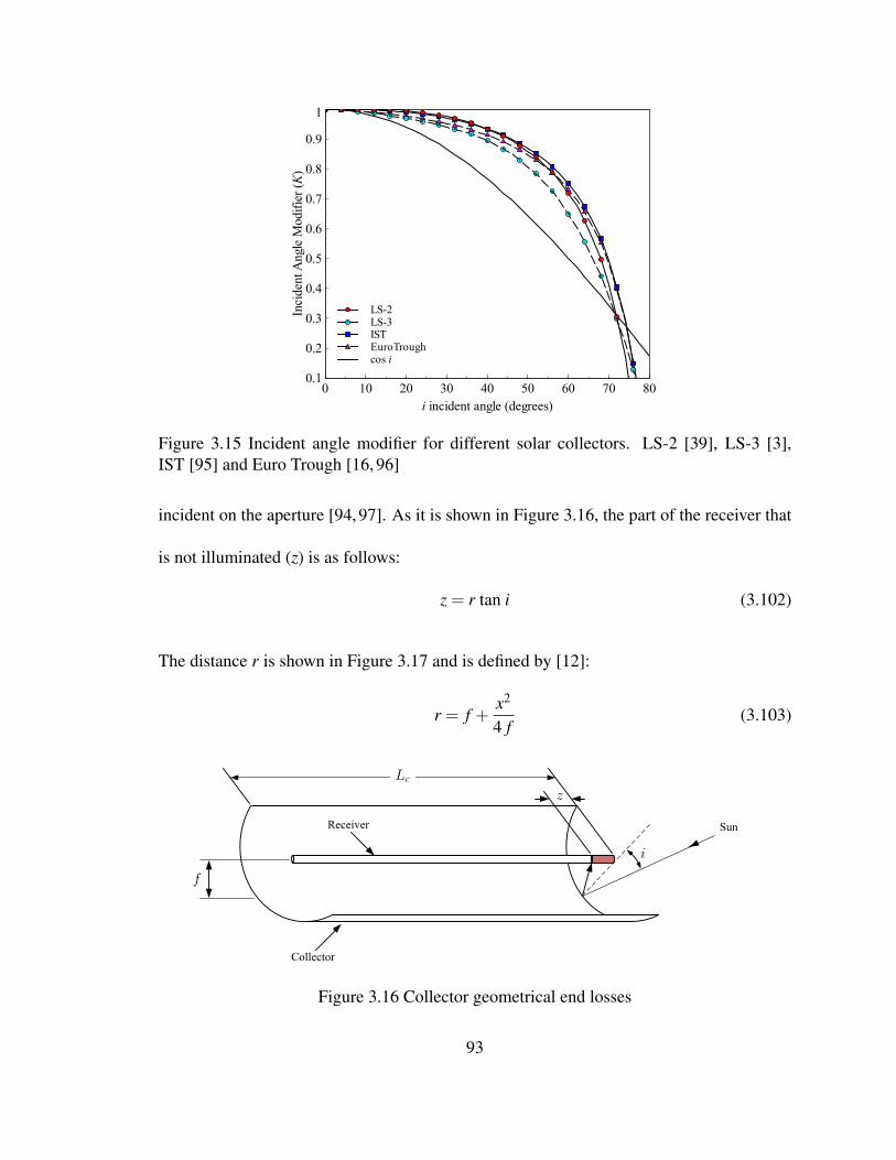
LS-2LS-3ISTEuroTroughcos i

Inci

dent

Ang

le M

odifi

er (K

)

0.1

0.2

0.3

0.4

0.5

0.6

0.7

0.8

0.9

1

i incident angle (degrees)0 10 20 30 40 50 60 70 80

Figure 3.15 Incident angle modifier for different solar collectors. LS-2 [39], LS-3 [3],IST [95] and Euro Trough [16, 96]

incident on the aperture [94, 97]. As it is shown in Figure 3.16, the part of the receiver that

is not illuminated (z) is as follows:

z = r tan i (3.102)

The distance r is shown in Figure 3.17 and is defined by [12]:

r = f +x2

4 f(3.103)

z

f

i

Lc

Sun

Collector

Receiver

Figure 3.16 Collector geometrical end losses

93

a

A

B

F

Focal Point

fr

' 'm

W=2

Figure 3.17 Parabola geometry for a rim angle of ϕm. Adapted from [30]

The fraction of the receiver that is illuminated is:

ψ (i) = 1− rLc

tan i (3.104)

Lippke et al. [5] proposed to take r = f . This assumption is widely used in other models

[8, 13] and leads to minimum end losses for certain geometric configuration. A previous

work developed by Gaul and Rabl [94] suggests the use of an average value of r. This

value is used in the present work and is given by:

r =1

w/2

∫ w/2

0

(f +

x2

4 f

)dx = f

(1+

w2

48 f 2

)(3.105)

Replacing the value of r, then, the collector geometrical end loss [94, 97] is:

ψ (i) = max(

0, 1− fLc

(1+

w2

48 f 2

)tan i

)(3.106)

94

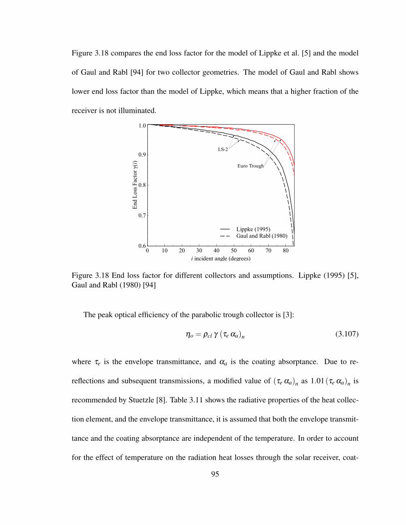
Figure 3.18 compares the end loss factor for the model of Lippke et al. [5] and the model

of Gaul and Rabl [94] for two collector geometries. The model of Gaul and Rabl shows

lower end loss factor than the model of Lippke, which means that a higher fraction of the

receiver is not illuminated.

Lippke (1995)Gaul and Rabl (1980)

Euro Trough

LS-2

End

Loss

Fac

tor γ

(i)

0.6

0.7

0.8

0.9

1.0

i incident angle (degrees)0 10 20 30 40 50 60 70 80

Figure 3.18 End loss factor for different collectors and assumptions. Lippke (1995) [5],Gaul and Rabl (1980) [94]

The peak optical efficiency of the parabolic trough collector is [3]:

ηo = ρcl γ (τe αa)n (3.107)

where τe is the envelope transmittance, and αa is the coating absorptance. Due to re-

reflections and subsequent transmissions, a modified value of (τe αa)n as 1.01(τe αa)n is

recommended by Stuetzle [8]. Table 3.11 shows the radiative properties of the heat collec-

tion element, and the envelope transmittance, it is assumed that both the envelope transmit-

tance and the coating absorptance are independent of the temperature. In order to account

for the effect of temperature on the radiation heat losses through the solar receiver, coat-

95

ing emittance was approximated by a polynomial function obtained by Forristall [6]. The

polynomial coefficients are shown in Table 3.12.

Other important properties for solar radiation losses are the glass envelope absorptance

and emissivity. In this models it is assumed that both of these radiative properties are

independent of the temperature; the envelope absorptance has a value of αe = 0.023 [100],

while the emissivity has an average value of εe = 0.90 [100]. Figure 3.19 shows the values

Table 3.11 Radiative properties of different heat collection elements (HCE). Adapted from[6]

Selective CoatingEnvelopeTransmittance

CoatingAbsorptance

CoatingEmittance

100 ºC 400 ºC

Luz Black Chrome 0.935 0.940 0.110 0.27

Luz Cermet 0.935 0.920 0.060 0.15

Solel UVAC Cermet a 0.965 0.960 0.070 0.13

Solel UVAC Cermet b 0.965 0.950 0.080 0.15

Solel UVAC Avg 0.965 0.955 0.076 0.14

Schott PTR®70 [98] 0.96 0.95 – 0.1

Table 3.12 Coating emittance of different solar receivers. Adapted from [6]

Selective Coating Coating Emittance (1)

Luz Black Chrome 5.333×10−4 (T +273.15)−0.0856

Luz Cermet 3.27×10−4 (T +273.15)−0.065971

Solel UVAC Cermet a 2.249 × 10−7 T 2 +1.039 × 10−4 T +0.05599

Solel UVAC Cermet b 1.565 × 10−7 T 2 +1.376 × 10−4 T +0.06966

Solel UVAC Avg 1.907 × 10−7 T 2 +1.208 × 10−4 T +0.06282

Schott PTR®70 (2) [99] 2.00 × 10−7 T 2 +0.062

(1) Temperature in ºC(2) At an absorber temperature of 400 °C the emittance uncertainty was ± 0.005

96

6.35 mm thick (Touloukian and DeWitt, 1972)12.7 mm thick (Touloukian and DeWitt, 1972) εe = 0.90

Emiss

ivity

of B

oros

ilica

te G

lass

0.2

0.3

0.4

0.5

0.6

0.7

0.8

0.9

1

Temperature (K)300 350 400 450 500 550 600 650 700 750 800

Figure 3.19 Effect of temperature on the emissivity of borosilicate glass for two thicknesses(6.35 and 12.7 mm). Values taken from [100]

of the emissivity for borosilicate glass at different thicknesses. The energy absorbed on the

solar receiver and the glass envelope is given by:

Qa−abs = ηo K (i) ϕ (i) SH I′bn (3.108)

and

Qe−abs = ρcl γ αe K (i) ϕSH ϕ (i) I′bn (3.109)

where ϕSH is the shading factor, with ϕSH = 0 for the collector aperture area totally shaded.

3.3 Numerical Solution

The partial differential equations (PDE) were discretized for steady state conditions by

using the finite difference method and taking into account the dependence of the thermal

97

properties on the temperature [101]. For the heat transfer fluid, the discretization by using

backward difference gave the following algebraic equation:

γi−1 Tf ,i−1−βi Tf ,i + τi = 0 i = 1,2, . . .N (3.110)

with

γi−1 =m f

∆zCp, f ,i−1

βi =m f

∆zCp, f ,i +π Nu f ,i k f ,i

τi =m f

∆z

[(V 2

f

2

)i−1

−

(V 2

f

2

)i

]+π Nu f ,i k f ,i Ta,i

Boundary nodes:

i = 0, Tf ,0 = Te (3.111)

For the absorber, the discretization was carried out by using central difference. The

algebraic equation obtained was as follows:

αi Ta, i−1−α+i Ta. i +α

′i Ta, i+1 +λq, i = 0 i = 1, 2, . . .N (3.112)

with

αi = Aaka, i

∆z2

α′i = Aa

ka, i+1

∆z2

α+i = αi +α

′i

98

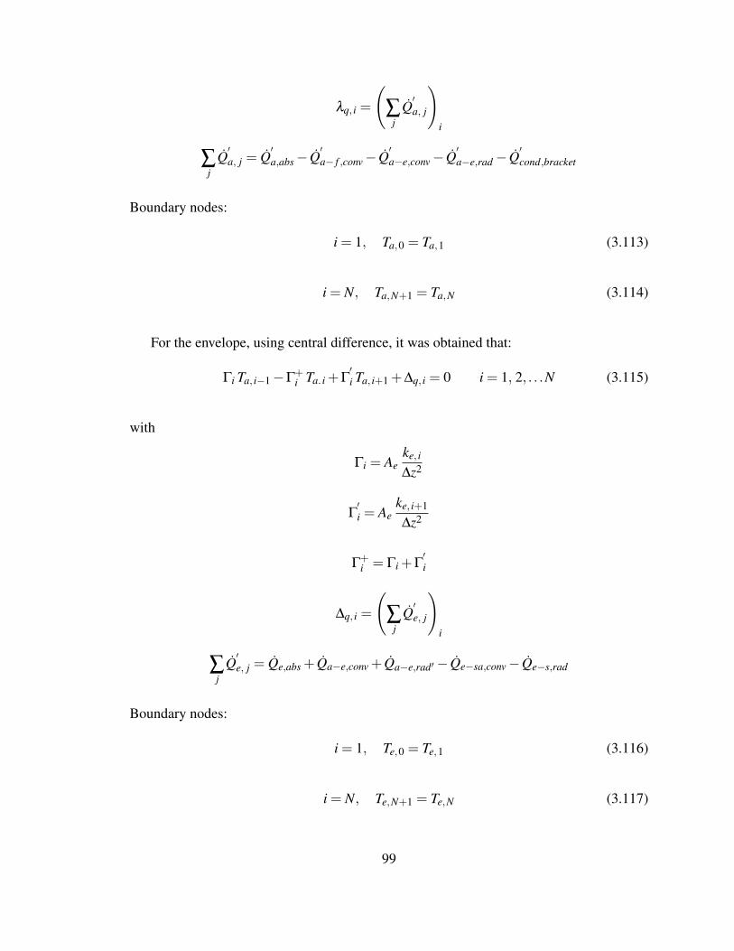
λq, i =

(∑

jQ′a, j

)i

∑j

Q′a, j = Q

′a,abs− Q

′a− f ,conv− Q

′a−e,conv− Q

′a−e,rad− Q

′cond,bracket

Boundary nodes:

i = 1, Ta,0 = Ta,1 (3.113)

i = N, Ta,N+1 = Ta,N (3.114)

For the envelope, using central difference, it was obtained that:

Γi Ta, i−1−Γ+i Ta. i +Γ

′i Ta, i+1 +∆q, i = 0 i = 1, 2, . . .N (3.115)

with

Γi = Aeke, i

∆z2

Γ′i = Ae

ke, i+1

∆z2

Γ+i = Γi +Γ

′i

∆q, i =

(∑

jQ′e, j

)i

∑j

Q′e, j = Qe,abs + Qa−e,conv + Qa−e,rad′− Qe−sa,conv− Qe−s,rad

Boundary nodes:

i = 1, Te,0 = Te,1 (3.116)

i = N, Te,N+1 = Te,N (3.117)

99

The nonlinear algebraic equations were written in Python 2.6 [34] and solved simul-

taneously by using a wrapper around MINPACK’s “hybrd” and “hybrj” algorithms [102].

The collector efficiency and thermal losses are calculated as follows:

ηc =m(ho, f −hi, f

)Ib Aap

(3.118)

Thermal Loss =

[∑

i

(Q′a−e,conv

)i+∑

i

(Q′a−e,rad

)i+∑

j

(Q′cond,bracket

)j

]∆z

Ib Aap(3.119)

3.4 Model Validation

In order to validate the heat transfer model, it was compared with experimental data

obtained from Sandia National Laboratories (SNL) [39]. In addition, to corroborate the

improvement in the correlations and radiation analysis proposed in this chapter, the numer-

ical model was also compared with the other solar receiver heat transfer models [6, 41].

The experimental results were for a solar collector assembly (LS-2) module placed at the

AZTRAK rotating platform at the SNL. Due to limitations in the experimental set up, a

2 inch diameter flow restriction device (solid plug) was centered in the inside diameter of

the absorber tube. Two different selective coatings were used in this test: black chrome

and cermet. Cermet has better radiative properties (low emissivity) at high temperatures

than black chrome, and does not oxidize if the vacuum is lost [39]. The Sandia test was

performed for both full sun and no sun condition and different scenarios for the annulus

of the heat collection element (HCE) : vacuum intact (the evacuated annulus pressure was

10−4 Torr), lost vacuum (annulus filled with ambient air), and glass cover completely re-

moved (bare tube). The three previous conditions were tested with the cermet coating but

broken annulus was not included for the black chrome coating case. All the conditions and

100

Table 3.13 Specifications for a SEGS LS-2 parabolic trough solar collector test. Data takenfrom [39]

Module Size 7.8 × 5 m

Rim angle 70◦

Reflectors 12 thermally sagged panelsSecond surface silveredLow iron glass (εc = 0.86 [103])

Aperture Area 39.2 m2

Focal Length 1.84 m

Concentration Ratio 71

Receiver (HCE) Evacuated tube design, metal bellows at each endAbsorber diameter: 70 mmLength: 4 m (2 per module at Sandia)Pyrex glass envelope : 115 mm diameterSelective coating: Cermet and Black chromei = 0, K (i) = 1, ϕ (i) = 1

Conditions of HCE Annulus Vacuum intact (the evacuated annulus pressure was 10−4

Torr)Lost vacuum (annulus filled with ambient air)Glass cover completely removed (bare tube)

Atmospheric Air Pressure 0.83 atm

Heat Transfer Fluid Syltherm 800

specifications used in the experimental test are summarized in Table 3.13. A silicone heat

transfer fluid (Syltherm 800) was used in the experimental set up. The properties for this

working fluid were fitted to the experimental data from [104] and a polynomial regression

was obtained for each property. The equations used for this fitting were:

Cp,s800 =3

∑n=0

Cp,n T n (3.120)

ρs800 =3

∑n=0

ρn T n (3.121)

101

ks800 =3

∑n=0

kn T n (3.122)

The coefficient obtained by the polynomial regression are shown in Table 3.14.

Table 3.14 Coefficients obtained by polynomial regression of thermal properties ofSyltherm 800. Experimental data taken from [104]

PropertyCoefficients, n

R2

0 1 2 3

Cp,n 1.574 1.707E-03 0.000 0.000 0.99ρn 953.164 -0.916 4.211E-04 -1.670E-06 0.99kn 0.138 -1.880E-04 0.000 0.000 0.99

All the results in this chapter were obtained by dividing the solar receiver into 12 seg-

ments, ∆x = 2/3m. This number of segments was selected according to a grid-independent

solution analysis. Figure 3.20 shows the results obtained for different collector segments

I = 950 W/m2

Vwind=0 m/sTamb=25 oCTin=300 oCFlow rate = 50 GPMHTF : Syltherm 800

Heat LossCollector Efficiency

Collector Efficiency (%)

64

65

66

67

68

Hea

t Los

s (W

/m2 )

63

64

65

66

Collector Segments0 2 4 6 8 10 12 14 16 18

Figure 3.20 Grid independent analysis for different collector segments, case: air in theannulus

102

with cermet coating as selective coating and air in the annulus. The results show that 12

elements are suitable for validation of the proposed heat transfer analysis.

3.5 Results and Discussion

The results obtained for the collector efficiency and thermal losses are shown in Figures

3.21-3.23. For the collector efficiency (Figure 3.21), the model follows the trends of the

experimental values and all the results are always inside the experimental error bars. As it

was expected, the higher efficiencies are obtained when the annulus is under vacuum, but in

both cases (air and vacuum) at high temperatures the collector efficiency drops gradually,

which is more notable for the black chrome coating as it is shown in Figure 3.21(b). This

is explained by the radiative properties of black chrome coating at high temperatures. For

the case of cermet coating, Figure 3.21(a), the model developed by Garcia-Valladares and

Velásquez [41] shows some discrepancies at low temperatures in the collector efficiency

due to their assumptions : negligible conduction at the ends of each trough and only ra-

diation heat losses take place between the receiver and the glass envelope for the case of

vacuum in the annular space (refer to [41] for more details). Those assumptions were not

made in the current model or NREL model. The proposed model and NREL model [6]

seem to obtain similar collector efficiencies values, but a detailed root mean square error

calculation (Table 3.15 and 3.16) shows that the proposed model achieved an improvement

as compared with the NREL and Garcia-Valladares and Velásquez models. The only case

without improvement was for black chrome coating with air in the annulus (RMSE of 0.855

% and 0.808 % for the proposed model and NREL model respectively), where there is not

much difference between the proposed and the NREL models.

103

Current ModelNREL Model (Forristall, 2003)García-Valladares and Velázquez Model, 2009Experimental values (Dudley et.al, 1994)Vacuum (Performance equation, Dudley et.al, 1994)Air (Performance equation, Dudley et.al, 1994)

Colle

ctor

Effi

cien

cy (%

)

50

55

60

65

70

75

80

Average Temperature Above Ambient (oC)0 100 200 300 400

(a) Cermet coating

Current ModelNREL Model (Forristall, 2003)Experimental values (Dudley et.al, 1994)Vacuum (Performance equation, Dudley et.al, 1994)Air (Performance equation, Dudley et.al, 1994)

Colle

ctor

Effi

cien

cy (%

)

50

55

60

65

70

75

80

Average Temperature Above Ambient (oC)0 100 200 300 400

(b) Black chrome coating

Figure 3.21 Comparison of collector efficiency calculated from the proposed model withexperimental data [39] and other solar receiver models [6, 41]

104

Current ModelNREL Model (Forristall, 2003)Experimental values (Dudley et.al, 1994)Vacuum (Performance equation, Dudley et.al, 1994)Air (Performance equation, Dudley et.al, 1994)

Ther

mal

Los

s (W

/m2 )

0

20

40

60

80

100

120

140

160

180

200

Average Temperature Above Ambient (oC)0 100 200 300 400

(a) Cermet coating

Current ModelNREL Model (Forristall, 2003)Experimental values (Dudley et.al, 1994)Vacuum (Performance equation, Dudley et.al, 1994)Air (Performance equation, Dudley et.al, 1994)

Ther

mal

Los

s (W

/m2 )

0

20

40

60

80

100

120

140

160

180

200

Average Temperature Above Ambient (oC)0 100 200 300 400

(b) Black chrome coating

Figure 3.22 Comparison of thermal losses calculated from the proposed model with exper-imental data [39] and other solar receiver models [6, 41], on-sun case

105

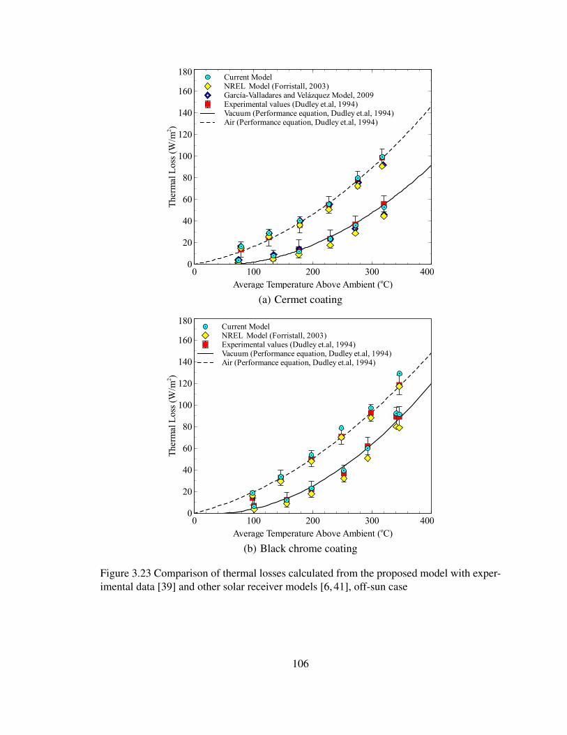
Current ModelNREL Model (Forristall, 2003)García-Valladares and Velázquez Model, 2009Experimental values (Dudley et.al, 1994)Vacuum (Performance equation, Dudley et.al, 1994)Air (Performance equation, Dudley et.al, 1994)

Ther

mal

Los

s (W

/m2 )

0

20

40

60

80

100

120

140

160

180

Average Temperature Above Ambient (oC)0 100 200 300 400

(a) Cermet coating

Current ModelNREL Model (Forristall, 2003)Experimental values (Dudley et.al, 1994)Vacuum (Performance equation, Dudley et.al, 1994)Air (Performance equation, Dudley et.al, 1994)

Ther

mal

Los

s (W

/m2 )

0

20

40

60

80

100

120

140

160

180

Average Temperature Above Ambient (oC)0 100 200 300 400

(b) Black chrome coating

Figure 3.23 Comparison of thermal losses calculated from the proposed model with exper-imental data [39] and other solar receiver models [6, 41], off-sun case

106

Table 3.15 Comparison of root mean square error (RMSE) between the proposed heat trans-fer model and other numerical models for the cermet coating case. Experimental data takenfrom [39], NREL model [6], García-Valladares and Velázquez Model [41]

ModelRMSE

ηc (%) Heat Losses (W/m2)

Vacuum (Sun)

Current model 1.012 10.255

NREL model 1.382 14.718

García-Valladares and Velázquez Model 1.433 —

Vacuum (Off Sun)

Current model — 2.414

NREL model — 6.004

García-Valladares and Velázquez Model — 4.671

Air (Sun)

Current model 1.225 8.959

NREL model 1.562 13.594

García-Valladares and Velázquez Model 2.292 —

Air (Off Sun)

Current model — 2.651

NREL model — 4.416

García-Valladares and Velázquez Model — 3.865

Figures 3.22 and 3.23 show the thermal losses calculated for the different models and

compared with the experimental values. As in the case of collector efficiency, the thermal

losses also showed a good agreement with the experimental results and most of the val-

ues are inside the experimental error bars. The RMSE analysis shows that the proposed

model gave thermal loss values closest to the experimental results as compared to those

obtained from the NREL and Garcia-Valladares and Velásquez models. The only excep-

107

Table 3.16 Comparison of root mean square error (RMSE) between the proposed heat trans-fer model and other numerical models for the black chrome coating case. Experimental datataken from [39], NREL model [6]

ModelRMSE

ηc (%) Heat Losses (W/m2)

Vacuum (Sun)

Current model 0.926 4.260

NREL model 1.191 9.650

Vacuum (Off Sun)

Current model — 1.978

NREL model — 7.230

Air (Sun)

Current model 0.855 13.196

NREL model 0.808 11.225

Air (Off Sun)

Current model — 4.714

NREL model — 2.667

tion was again for the black chrome coating, for which the NREL model achieved better

RMSE (11.225 W/m2 and 2.667 W/m2 for on-sun and off-sun case respectively, air in the

annulus scenario) than the proposed model (13.196 W/m2 and 4.714. W/m2 for the current

model respectively). In this case our model shows higher heat losses at temperatures above

ambient of 350 ◦C or higher. It is difficult to say which model is more accurate, although

we feel our model is more conservative.

The third scenario, with the glass envelope removed (bare tube) and the surrounding air

in direct contact with the absorber tube, leads to highest thermal losses as expected. This

scenario is possible in the solar power plants during regular operation when the glass tube

108

gets broken. The heat transfer analysis for this scenario quantifies how much the collector

efficiency is degraded. For this case, wind speed takes an important role in the thermal

losses and therefore in the collector efficiency as well. Naeeni and Yaghoubi [105, 106]

analyzed the wind flow and thermal field around the receiver tube. They concluded that the

local Nusselt distribution around the receiver tube is different from the cross flow condition.

Given that in the proposed model, the convective heat losses were calculated for a cylinder

in cross flow, it can be concluded that for forced convection (Vwind > 0) , the model will

overpredict thermal losses and underpredict collector efficiency. This can be seen in Figure

3.24 (ς = 1). Forristall [6] recommended to include in his model half of the convective

losses (ς = 0.5) to reduce the overestimation of thermal losses by convection. In this paper,

after a fitting analysis, it was found that a reduction of 41.8 % in heat convection losses

(ς = 0.582) leads to good results. Figure 3.24 compares the results obtained for different

heat convection factors. In order to compare the different heat convection factors, RMSE

was calculated for each factor. The results obtained are shown in Table 3.17; the lowest

RMSE was obtained for the factor proposed in this study, ς = 0.582.

Table 3.17 Comparison of root mean square error (RMSE) for different heat loss convectionfactors

ς Heat Loss (W/m2) ηc (%)

1.0 Regular model 91.62 13.12

0.5 Recommended by Forristall [6] 32.75 5.78

0.582 Proposed model 27.80 3.92

109

ζ = 0.582, Current modelζ = 0.5, Recommended by Forristall (Forristall, 2003)ζ = 1.0, Regular Model

Calc

ulat

ed C

olle

ctor

Effi

cien

cy (%

)

0

20

40

60

80

100

Experimental Collector Efficiency (%)0 20 40 60 80 100

(a) Collector efficiency

ζ = 0.582, Current modelζ = 0.5, Recommended by Forristall (Forristall, 2003)ζ = 1.0, Regular Model

Calc

ulat

ed T

herm

al L

oss (

W/m

2 )

0

100

200

300

400

500

600

Experimental Thermal Loss (W/m2)0 100 200 300 400 500 600

(b) Thermal loss

Figure 3.24 Comparison of theoretical and experimental [39] collector efficiency and ther-mal losses obtained for different heat convection loss factors

110

3.6 Non-Linear Regression Heat Loss Model

The proposed equation for the heat losses model is as follow:

QHL (W/m) = ψo +ψ1(Tf −T∞

)+ψ2 T 2

f +ψ3 T 3f

+Ibn K cos i[ψ4 +ψ5 T 2

f]+V n

wind[ψ6 +ψ7

(Tf −T∞

)](3.123)

with

Tf =Tf ,i +Tf ,o

2(3.124)

This equation is based on the correlation proposed by Price [11], although slight modi-

fications were introduced in the original equation. The conditions and parameters used for

the heat losses calculation are presented in Table 3.18.

Table 3.18 Specifications used for the heat loss model

Solar Collectors LS-2 and LS-3

Inlet Temperature (◦C) 50, 100,150,. . .400

Beam Radiation (W/m2) 0, 250, 500, 750, 1000

Ambient Temperature (◦C) 15, 30, 45

Receiver (HCE) Selective coating: Universal Vacuum Air Collector(UVAC) [6]i = 0◦, 15◦, 30◦, 45◦, 60◦, 75◦, 90◦

SH = 1

Conditions of HCE Annulus Vacuum intact (the evacuated annulus pressure was10−4 Torr)Lost vacuum (annulus filled with ambient air)

Atmospheric Air Pressure 1 atm

Heat Transfer Fluid VP-1

Mass Flor rate (kg/s) 8

111

Table 3.19 Heat loss correlation coefficients

CoefficientsLS-2 LS-3

Vacuum Air Vacuum Air

ψo 1.868 -2.720 1.930 -3.229ψ1 2.515×10−1 1.028 2.498×10−1 1.033ψ2 -1.080×10−3 -1.165×10−3 -1.097×10−3 -1.201×10−3

ψ3 6.639×10−6 6.700×10−6 6.671×10−6 6.747×10−6

ψ4 1.771×10−4 -3.541×10−3 8.556×10−5 -4.596×10−3

ψ5 4.398×10−8 1.771×10−8 5.569×10−8 2.784×10−8

ψ6 -8.087×10−1 -3.686 -8.401×10−1 -3.503ψ7 3.543×10−2 1.605×10−1 3.555×10−2 1.603×10−1

n 3.598×10−1 3.536×10−1 3.537×10−1 3.533×10−1

R2 0.9998 0.9996 0.9998 0.9996

RMSE 1.64 4.00 1.69 4.01

The correlation coefficients for different conditions in the receiver annulus are shown in

Table 3.19. Table 3.19 also shows the coefficient of determination, R2, which is a measure

of how well the heat losses can be predicted by the proposed correlation, and the root mean

square error (RMSE). The results show that the proposed fitting Equation 3.123 predicts

the heat losses for LS-2 and LS-3 solar collectors very accurate. This is corroborated

in Figure3.25 by plotting the heat losses obtained from the non-linear regression and the

proposed model.

3.7 Conclusions

A comprehensive heat transfer model for thermal analysis of parabolic trough solar

receivers was developed. The proposed model included a detailed radiative heat transfer

analysis and more accurate heat transfer correlations. The results obtained showed good

agreement with experimental data and in comparison with other heat transfer models, the

proposed model presented in general lower RMSE values and better performance, espe-

112

LS-2LS-3

Regr

essio

n H

eat L

oss (

W/m

)

0

50

100

150

200

250

300

350

400

450

Modeled Heat Loss (W/m)0 50 100 150 200 250 300 350 400 450

(a) Vacuum

LS-2LS-3

Regr

essio

n H

eat L

oss (

W/m

)

0

100

200

300

400

500

600

700

800

Modeled Heat Loss (W/m)0 100 200 300 400 500 600 700 800

(b) Air

Figure 3.25 Comparison of heat losses obtained from the non-linear correlation (Equation3.123) and the proposed model

cially for the heat transfer losses. For the case of bare tube (glass envelope broken), it was

found that a factor of 0.418 in convective heat losses leads to improvement in the perfor-

mance of the heat transfer model. Based on the results obtained, it is concluded that this

model is suitable for the calculation of heat losses and collector efficiency under different

flow, selective coating and operating conditions.

A non-linear regression model was obtained for LS-2 and LS-3 solar collectors. This

model is very useful for predicting the heat losses in a solar collector under different radi-

ation and meteorological conditions without using the proposed comprehensive model.

113

Chapter 4

Power Block

4.1 Introduction

The power block commonly used in concentrating solar thermal power plants is a Re-

generative Rankine Cycle [13, 16]. The thermodynamic cycle is shown in Figure 4.1. The

heat transfer fluid (HTF) passes through three heat exchangers (simplified model): super-

heater, boiler and preheater. In the preheater, which is normally a shell and tube type heat

exchanger, compressed water coming from closed feedwater heater (CF-1) is heated up

until saturated liquid condition is reached. Then, the saturated liquid flows through the

boiler where a change of phase from liquid to vapor occurs. The boiler (steam generator) is

a shell-and-tube heat exchanger with the HTF entering the tube side and liquid feedwater

flowing through the shell side. After the boiler, the saturated vapor goes to the superheater

where additional energy is added to the steam, bringing it to a superheated vapor condi-

tion. This heat exchanger is a shell-and-tube type as well. The superheated steam (10) is

expanded through the high pressure turbine.

Two extractions, 11 and 12, are taken from the high pressure turbine to the closed

feedwaters (CF-1, CF-2). Closed feedwater heaters are shell-and-tube-type recuperators

[52], which are used to increase the feedwater temperature through condensation of the

extracted steam.

114

DP CP

CTP

1

23456

789

10

11 12

13

14

15

16 17 18

19

2021222324 24' 23' 22' 21'

20'

25

a

b

c

Heat Transfer Fluid (HTF)

Generator

Reheater HE

Boiler HE

Preheater HE

Superheater HE High Pressure Turbine

Low Pressure Turbine

CF-1 CF-2

OF

CF-3 CF-4 CF-5

Cooling Tower

C

CF: Closed feedwaterOF: Open feedwater (Deaerator)C: CondenserCP: Condenser pumpDP: Deaerator pump

CW1

CW2

CW3

9f

9g

b’

a’

Figure 4.1 Regenerative Rankine cycle configuration

115

The thermal efficiency of the cycle is increased by including closed feedwaters, but

the optimum number of heaters is based on economical optimization, and for this case an

optimum of five heaters is recommended [107,108]. The remaining steam (13) is reheated;

the reheat is used to allow higher boiler pressures without low-quality steam problems at

the turbine exhaust pressure and therefore an increase in the overall thermal efficiency of

the cycle is achieved. The reheated steam (14) is then expanded into the low pressure

turbine; four extractions, (15)-(18), are bled to the closed feedwaters (CF-3, CF-4, CF-5)

and an open feedwater (OF). Open feedwaters are a direct contact-type heat exchanger [52]

in which streams at different temperatures are mixed to form a stream at an intermediate

temperature at saturated liquid condition (6).Open feedwaters are also used for removing air

and other dissolved gases which can cause corrosion problem or decrease the performance

of the cycle. The exhaust turbine stream (19) is mixed with the feedwater coming from

the trap in the closed feedwater 5 (CF-5). A trap is a valve that permits only liquid to pass

through to a region of lower pressure [52]. The mixture goes to the condenser, a shell-and-

tube heat exchanger, where a change of phase from mixture to saturated liquid takes places.

The feedwater (1) leaving the condenser (Saturated liquid condition) is pumped to the open

feedwater pressure though the condenser pump. The feedwater is preheated by the closed

feedwaters (CF3, CF4 and CF5) until it reaches the open feedwater (5). Saturated liquid

at the exit of the open feedwater (6) is pumped at boiler pressure and preheated by closed

feedwaters (CF1 and CF2) and finally returns to the preheater (9).

Initially, mass and energy balance, under steady state conditions, was carried out in

each component of the cycle and mass flow rate, temperature and pressure were obtained

116

for each stream. The thermodynamic cycle was then modeled for partial load conditions.

These partial load conditions are present throughout the day due to the intermittent energy

absorbed by the solar field. These conditions affect the temperature and mass flow rate

of the HTF entering the power block. The mass flow rate is varied for the cases in which

the HTF temperature is held constant. For partial load conditions in heat exchangers the

approximation developed by Patnode [13] was used:

UAUAre f

=

(mo

mo,re f

)0.8

(4.1)

where UA and UAre f are the product of the overall heat transfer coefficient, U , and the

heat transfer area, A, for the current and reference conditions respectively, and mo and

˙mo,re f are the mass flow rates of the outer fluid in the heat exchanger for the current and

reference conditions respectively. This approach is based on Colburn equation for fluids

with constants properties and it assumes that the mass flow rates of the inner and outer

fluids remain in the same proportion at partial load conditions as at the reference load.

mi

mo=

˙mi,re f

˙mo,re f(4.2)

The thermodynamic properties of water and steam were implemented in Python 2.6 [34]

by using the international-standard IAPWS-IF97 steam tables [109]. The analysis for each

component of the cycle is developed below. For all the heat exchangers it is assumed that:

• The heat exchangers operate under steady state and steady flow conditions

• Heat transfer losses to the ambient are negligible

117

• There is no heat generation in the heat exchangers

• Pressure drop is negligible

4.2 Reheater and Superheater

Superheater and reheater increase the temperature of the saturated or near saturated

steam in order to increase the thermodynamic efficiency of the Rankine cycle [110]. They

are shell-and-tube heat exchangers whose main difference is the operating pressure. In the

superheater, thermal energy is added to the steam coming from the boiler to bring it to

superheated conditions. For the reheater, steam coming from the high pressure turbine exit

is reheated to avoid problems with the steam quality leaving the low pressure turbine and

increase the overall efficiency of the Rankine cycle. The following assumptions are made

for the superheater and reheater heat exchangers:

• The steam entering the superheater (stream 9g) is at saturated vapor conditions

• The temperature of the stream leaving the superheater is given by: T10 = Ta−∆Tpinch

(Figure 4.2)

• The temperature of the stream leaving from the reheater is : T14 = Ta−∆Tpinch

Figure 4.3 shows a schematic of the reheater and superheater. The heat transfer fluid

(HTF) coming from the solar field heats up the steam leaving the boiler (superheater) or

high pressure turbine (reheater). Counterflow arrangement, (one-shell pass and one-tube

pass) is assumed and the effectiveness–NTU method is used for all the heat exchangers.

118

¢ Tmin

¢ Tmin

Heat Transfer FluidWater and Steam

Tem

pera

ture

Entropy

9

9f 9g

10

aa0

b0

b

Pinch Point

PreheatVaporizationSuperheat

9¡ 9f

9f ¡ 9g

9g ¡ 10

Figure 4.2 Steam generation process

This method is based on a dimensionless parameter called the heat transfer effectiveness ,

defined as [111]:

ε =Q

Qmax=

Actual heat transfer rateMaximum posible heat transfer rate

(4.3)

HTFi

Steami

Steamo

HTFo

Figure 4.3 Reheater and superheater heat exchanger

119

The actual heat transfer rate can be determined from the energy balance on the hot

(HTF) and cold (steam) fluids as follows:

Q =CHT F (THT Fi−THT Fo) (4.4)

Q =CSteam (TSteamo−TSteami) (4.5)

with the heat capacity rates defined as:

CHT F =mHT F (hHT Fi−hHT Fo)

THT Fi−THT Fo

(4.6)

CSteam =mSteam (hSteamo−hSteami)

TSteamo−TSteami

(4.7)

where mHT F is the mass flow rate of the heat transfer fluid, and mSteam is the mass flow rate

of the steam. The mass balance for this feedwater heater is:

mHT Fo = mHT Fi (4.8)

mSteamo = mSteami (4.9)

The maximum temperature difference in a heat exchanger is the difference between the

inlet temperatures of the heat transfer fluid (hot) and the inlet steam (cold).

∆Tmax = THT Fi−TSteam,i (4.10)

The maximum heat transfer rate in a heat exchanger is reached when the steam is heated

to the inlet temperature of the hot fluid or the HTF is cooled to the inlet temperature of the

steam. These two limiting conditions will not be reached simultaneously unless the heat

capacity rates of the HTF and steam are identical (CHT F = CSteam) [111]. The fluid with

120

the smaller heat capacity rate will reach the larger temperature difference, therefore, the

maximum possible heat transfer rate in a heat exchanger is given by:

Qmax =Cmin(THT Fi−TSteam,i

)(4.11)

and

Cmin = min (CHT F , CSteam) (4.12)

Then, once the effectiveness of the heat exchanger is known, the actual rate of heat

transfer is as follows:

Q = ε Cmin(THT Fi−TSteam,i

)(4.13)

The effectiveness of a heat exchanger depends on the geometry of the heat exchanger as

well as the flow arrangement [111]. Two parameters typically involved in the effectiveness

relation of a heat exchanger are:

ε = f(

UACmin

,Cmin

Cmax

)(4.14)

where UA/Cmin, also known as the number of transfer units NTU , is a measure of the

heat transfer surface area A, and Cmin/Cmax is the dimensionless capacity ratio, c. For a

counterflow arrangement (one-shell pass and one-tube pass) the effectiveness is as follows

[111]:

ε =1− exp [−NTU (1− c)]

1− c exp [−NTU (1− c)](4.15)

121

A special case it is presented when c= 1, for this case the effectiveness is simplified as [56]:

ε =NTU

1+NTU(4.16)

The effectiveness can be also expressed in terms of the maximum heat transfer rate:

ε =CHT F (THT Fi−THT Fo)

Cmin(THT Fi−TSteam,i

) (4.17)

or

ε =CSteam (TSteamo−TSteami)

Cmin(THT Fi−TSteam,i

) (4.18)

At partial load conditions the product of the overall heat transfer coefficient, U , and the

heat transfer area, A, is given by [112]:

UA′ =UA(

m′HT Fi

mHT Fi

)0.8

(4.19)

where UA′ is the new product of the overall heat transfer coefficient and the heat transfer

area calculated at the new mass flow rate m′HT Fi.

4.3 Boiler

The boiler is a heat exchanger in which the feedwater changes phase from liquid to

vapor at constant temperature and pressure [111]. The boiler (Figure 4.4) is shell-and-

tube type heat exchanger with the HTF entering the tube side and liquid feedwater flowing

through the shell side. The following assumptions are made to the analysis of the boiler

heat exchanger:

122

• The feedwater stream entering the boiler (stream 9 f ) is at saturated liquid conditions

• The temperature of the HTF stream leaving the boiler is given by: Tb′ = Tsat @T=T9 +

∆Tpinch (Figure 4.2)

9g

9fb0

a0

HTF

Feedwater

Steam

HTF

Figure 4.4 Boiler heat exchanger

The actual heat transfer rate at the boiler is as follows:

Qboiler =CHT F(THT Fa′ −THT Fb′

)(4.20)

or

Qboiler = mFeedwater (hSteam−hFeedwater) = mFeedwater h f g @T=T9 (4.21)

The feedwater coming from the preheater absorbs a large amount of heat at constant

temperature during the phase-change process. The heat capacity rate of the steam during

the phase-change process approaches infinity since the temperature change is zero [111].

123

The minimum heat capacity rate is obtained from the HTF and the dimensionless capacity

ratio is defined as:

cboiler =Cmin,boiler

Cmax,boiler= 0 (4.22)

with Cmin defined as:

Cmin,boiler =CHT F =mHT F

(hHT Fa′ −hHT Fb′

)THT Fa′ −THT Fb′

(4.23)

The mass balance for the boiler is as follows:

mHT Fb′ = mHT Fa′ (4.24)

mSteam = mFeedwater (4.25)

The maximum heat transfer rate is given by:

Qboiler,max =Cmin(THT Fa′ −Tsat @T=T9

)(4.26)

The effectiveness is as follows [111]:

εboiler = 1− exp (−NTUboiler) (4.27)

or

εboiler =CHT F

(THT Fa′ −THT Fb′

)Cmin

(THT Fa′ −Tsat @T=T9

) (4.28)

εboiler =mFeedwater h f g @T=T9

Cmin(THT Fa′ −Tsat @T=T9

) (4.29)

124

At partial load conditions the product of the overall heat transfer coefficient, Uboiler,

and the heat transfer area, Aboiler, is given by [112]:

(UA)′boiler = (UA)boiler

(m′HT Fa′

mHT Fa′

)0.8

(4.30)

where (UA)′boiler is the new product of the overall heat transfer coefficient and the heat

transfer area of the boiler calculated at the new mass flow rate m′HT Fa′. The HTF return

temperature and mass flow rate are calculated as:

mHT F,rec = mHT F + mHT F,superheater (4.31)

hHT F,rec =mHT F hHT F,a + mHT F,superheater hHT F,c

mHT F + mHT F,superheater(4.32)

THT F,rec = f (hHT F,rec) (4.33)

4.4 Preheater

The preheater (Figure 4.5) is a shell and tube exchanger whose main goal is to bring

the entering feedwater to saturated liquid conditions. In order to simplify the analysis, the

preheater is assumed to be of variable area (this assumption is also adopted by Patnode

[13]) at partial load conditions so that the exiting stream 9 f is always at saturated liquid

condition. This assumption reduces the number of guess variables to be solved at partial

load conditions and does not have much effect on the performance of the cycle.

125

9fb0

b 9

HTF

Feedwater

Feedwater

HTF

Figure 4.5 Preheater heat exchanger

The actual heat transfer rates for the hot (HTF) and cold (feedwater) fluids is as follows:

˙Qpreheater = mHT F(hHT Fb′ −hHT Fb

)(4.34)

Qpreheater = mF(h9 f −h9

)(4.35)

where h9 f = h f @P=P10 and mF is the mass flow rate of the feedwater. The mass balance for

the preheater is:

mHT Fb = mHT Fb′ (4.36)

mFeedwater,9 = mFeedwater,9 f (4.37)

4.5 Closed Feedwater

Closed feedwater heaters are shell and tube heat exchangers, in which the steam bled

from the turbine condenses on the shell side whereas the feedwater stream is heated on the

tube side. The condensate is removed by using a trap and is allowed to pass to a feedwater

126

heater operating at lower pressure or into the condenser (stream 20’) [52]. Normally closed

feedwaters include three heat transfer zones as follows [113]:

• Desuperheating zone where the steam is cooled to its saturation temperature

• Condensing zone where the steam is condensed to saturated liquid condition at con-

stant pressure and temperature

• Subcooling zone where the liquid is cooled below its saturation temperature

It is assumed that the closed feedwater heaters are always working at the condensing zone

and the condensed water leaving the closed feedwater is at the saturated liquid condition.

The terminal temperature difference, which is the temperature difference between the sat-

uration temperature at the extraction pressure and the feedwater temperature leaving the

closed feedwater heater, is assumed as 2.8 ◦C at reference conditions [114]. The energy

and mass balance for the closed feedwater heater 2 (CF-2, Figure 4.6) are detailed below.

Initially thermodynamic properties of the stream 12’ (mixture) are calculated as:

h12′ =1

m12′[h24′ m24′+h12 m12] (4.38)

m12′ = m24′+ m12 (4.39)

The temperature of stream 12’ is given by:

T12′ = T (P12, h12′) (4.40)

127

78

12

23'

24'

CF-2

23

12'

Trap

Figure 4.6 Closed feedwater heater

The mass balance shows that m8 = m7, m23 = ˙m12′ , and m23′ = m23. For the stream after

the trap, stream 23’, the enthalpy is h23′ = h f @P=P12 and the energy balance is as follows:

m12′ h12′+ m7 h7− m8 h8− m23 h23 = 0 (4.41)

The actual heat transfer rate at the closed feedwater is then calculated as:

QCF−2 =CF,7−8 (T8−T7) (4.42)

QCF−2 = m12′ (h12′−h23) (4.43)

The analysis for the closed feedwater is similar to the boiler analysis previously per-

formed.

cCF−2 =Cmin,CF−2

Cmax,CF−2= 0 (4.44)

with Cmin defined as:

Cmin,CF−2 =CF,7−8 =m7 (h8−h7)

T8−T7(4.45)

128

The maximum heat transfer rate is given by:

QCF−2,max =Cmin (T12′−T7) (4.46)

The effectiveness is as follows [111]:

εCF−2 = 1− exp (−NTUCF−2) (4.47)

or

εCF−2 =CF,7−8 (T8−T7)

Cmin (T12′−T7)(4.48)

εCF−2 =m12′ (h12′−h23)

Cmin (T12′−T7)(4.49)

At partial load conditions the product of the overall heat transfer coefficient, UCF−2,

and the heat transfer area, ACF−2, is given by [13]:

(UA)′CF−2 = (UA)CF−2

(m′7m7

)0.8

(4.50)

where (UA)′CF−2 is the new product of the overall heat transfer coefficient and the heat

transfer area of the closed feedwater (CF-2) calculated at the new mass flow rate m′7.

4.6 Open Feedwater (Deaerator)

Open feedwater heaters are direct contact-type heat exchangers [52], which are more

efficient than closed feedwaters (Figure 4.7). In this feedwater heater, streams at different

temperatures and same pressure are mixed to achieve stream exiting at the saturation condi-

tion corresponding to the inlet pressure. Open feedwater heaters (Deaerator) are also used

129

for removing the air and other dissolved gases which can cause corrosion problems. The

mass and energy balance are obtained as:

m6 = m15 + m5 + m23′ (4.51)

h15 m15 +h5 m5 +h23′ m23′−h6 m6 = 0 (4.52)

56

15

23'

Figure 4.7 Open feedwater heater

4.7 Turbine

The proposed regenerative Rankine cycle uses two turbines: high pressure and low

pressure turbine; the high pressure turbine has two stages while the low pressure turbine

has five stages. Reheat is applied between the last stage of the high pressure turbine and

the first stage of the low pressure turbine. The reheat pressure was selected based on the

optimization analysis carried by Habib et al. [115] and Dincer and Al-Muslin [116]. They

concluded that the optimum reheat pressure should be between 19-20% of the boiler pres-

sure.

130

For both turbines the constant efficiency method [114] was employed to calculate the

entropy at the exiting stream of each stage. The optimum pressure at each extraction was

determined by dividing the total isentropic drop in equal parts according to the number of

stages (Figure 4.8). This configuration leads to optimum turbine performance [108, 113].

hi

h1

h2

h4

ho

Pi

P1

P2

P3

P4

Po

¢hs

15¢hs

15¢hs

15¢hs

15¢hs

15¢hs

h3

Entropy

Ent

halp

y

Figure 4.8 Enthalpy-entropy diagram of steam expansion in a multi-stage turbine (5 stages)

The procedure for modeling the high pressure turbine is shown below (Figure 4.9).

Initially, the properties at the inlet stream are calculated. The exit pressure is determined

from the optimum reheat pressure as previously explained.

P13 = fb P (4.53)

with 0.19≤ fb ≤ 0.2. The value of fb is selected so that the minimum steam quality at the

exit is x19 ≥ 0.9.

The isentropic enthalpy drop is calculated as:

∆hs,T = h10−h12,s (4.54)

131

13

To Reheater HE

From Boiler

10

1112

To CF-1 To CF-2

Figure 4.9 High pressure turbine (2 stages)

The isentropic enthalpy drop in each stages is calculated by dividing the total isentropic

enthalpy drop by the number of stages. The isentropic enthalpy is calculated at each ex-

traction as:

h11,s = h10−∆hs,T/2 (4.55)

h12,s = h13,s = h11−∆hs,T/2 (4.56)

The optimum extraction pressures are given by:

P11 = P (h11,s, s10) (4.57)

P12 = P13 = P (h12,s, s10) (4.58)

132

The enthalpy at each exiting stream is calculated by using the constant efficiency method

[114].

h11 = h10−ηH,T (h10−h11,s) (4.59)

h12 = h13 = h10−ηH,T (h10−h12,s) (4.60)

The steam flow to the steam turbine is controlled by the steam control valves. There are

two main methods to vary the steam flow though the steam turbine [117]:

• changing the position of the turbine control valves

• changing the steam pressure upstream from the turbine valves by keeping them in a

fixed position

In the fixed boiler pressure control the turbine governor valve is used to control the power

output while boiler pressure is kept almost constant. This method works under rapid load

changes but large thermal stresses are induced due to the inlet steam temperature fluctuation

[118]. For sliding pressure control, boiler pressure is used to control the output power while

the turbine governor valves is kept wide open. Although this control strategy produces

minimal thermal stress, the response of the system is slow and the thermal efficiency is

lower compared to the fixed boiler pressure control method [16]. In this analysis, sliding

pressure control is assumed since it has better performance for large load changes [16],

which is commonly the case in solar power plants owing to the intermittency of the solar

irradiation.

133

The calculation of the transient operating conditions for each stage of the turbine is

done starting with the last stage and up to the first stage. At partial load conditions, the

pressure drop at each stage is calculated by using Stodola Law1 [107]:

P2i −P2

o

P2i,re f −P2

o,re f=

(m

mre f

)2

(4.61)

where Pi is the inlet pressure of the stage, Po is the outlet pressure of the stage, Pi,re f is

the inlet pressure of the stage at reference conditions, Po,re f is the outlet pressure of the

stage at reference conditions, and m/mre f is the throttle flow ratio. The turbine efficiency

is affected at partial load conditions as well, specifically there is a reduction in the turbine

efficiency given by:

ηt = (1−R)ηt,re f (4.62)

The reduction factor R (Figure 4.10) is as follows2 [119]:

R = 0.191−0.409(

mmre f

)+0.218

(m

mre f

)2

(4.63)

4.8 Pump

A pump is a device to move or compress liquids [52]. The proposed thermodynamic

cycle has two pumps: condenser pump and open feedwater pump. The condenser pump

increases the pressure from the cycle low pressure to the open feedwater pressure while the

open feedwater pump increases the pressure from the open feedwater pressure to the boiler

1No correction factor for temperature is included because the sliding pressure keeps the steam inlettemperature almost constant

2Condensing turbine with one governing stage and 3600 rpm

134

ηt /η

t,o (%)

0.84

0.86

0.88

0.90

0.92

0.94

0.96

0.98

1.00

Redu

ctio

n of

Tur

bine

Effi

cien

cy (%

)

0

2

4

6

8

10

12

14

16

18

m/mref

0 0.1 0.2 0.3 0.4 0.5 0.6 0.7 0.8 0.9 1

Figure 4.10 Effect of throttle flow ratio on the turbine efficiency

pressure. The work input required to compress the feedwater is taken into consideration

for calculation of the net work obtained from the thermodynamic cycle, since this electric

work is subtracted from the net electric work obtained from the turbines.

The pumps are assumed to work under steady conditions and heat losses to the sur-

roundings are negligible. The mass and energy balance are as follows (Figure 4.11):

mFeedwateri = mFeedwatero (4.64)

Feedwateri

Feedwatero

Figure 4.11 Pump

135

The exiting enthalpy is given by:

hFeedwatero = hFeedwaterii +

(hFeedwatero,s−hFeedwaterii

)ηpump

(4.65)

with hFeedwatero,s = h (PFeedwatero, sFeedwateri). The pump work is then:

Wpump = mFeedwateri (hFeedwatero−hFeedwaterii) (4.66)

At partial load conditions the efficiency of the pump is affected by the variation of mass

flow rate. The pump efficiency is defined by [5]:

ηpump

ηpump,re f= emo +2 (1− emo)

mFeedwateri

mFeedwateri,re f

− (1− emo)

(mFeedwateri

mFeedwateri,re f

)2

(4.67)

where ηpump,re f is the efficiency of the pump at reference conditions. For constant speed,

Lippke [5] recommends to use a value of emo = 0. Figure 4.12 shows the effect of throttle

flow ratio on the pump efficiency.

η pump/η

pump,o

0.1

0.2

0.3

0.4

0.5

0.6

0.7

0.8

0.9

1.0

m/mref0 0.1 0.2 0.3 0.4 0.5 0.6 0.7 0.8 0.9 1

Figure 4.12 Effect of throttle flow ratio on the pump efficiency

136

4.9 Condenser

The condenser is a two phase flow heat exchanger. The heat generated by the steam

phase change from vapor to liquid is removed by a coolant. The shell and tube condenser

has the coolant flowing on the tube side and the steam on the shell side. Cooling water

is commonly used as the coolant in the solar power plants although problems with water

shortages have brought air cooled condensers as an alternative [120]. The mass and energy

balance for the condenser are as follows (Figure 4.13):

Qc = m25 (h25−h1) (4.68)

m25 = m1 (4.69)

where h1 = hsat@P=P25 . The efficiency of the Rankine cycle is affected by the condenser

pressure; at a fixed boiler pressure the condenser pressure should be kept as low as possible

[52]. The condenser temperature depends on the cooling method employed to remove the

latent heat to the surroundings. The minimum ambient temperature is given by the wet

bulb temperature; thus, most of the solar power plants use cooling tower which keeps the

1

25Steam

Feedwater

Figure 4.13 Schematic of the condenser

137

cooling water temperature at values near this temperature by evaporation process. For sites

with water shortages, air cooled condensers can be used. Air cooled condensers are limited

to the dry bulb temperature of the air which decreases the thermal efficiency of the power

block. Two types of coolants were considered in this study: water and air. For both cooling

fluids, preliminary design to meet the thermal requirements of the condenser and hourly

simulations of operations were performed. A detailed analysis of the cooling methods and

their integration with the condenser is shown below.

4.9.1 Cooling Tower

Cooling towers are widely used in industrial processes to remove waste heat. Two types

of cooling towers exist: natural and mechanical draft. In this simulation mechanical draft

cooling tower with air and water in counterflow is analyzed.

A cooling tower cools water by a combination of heat and mass transfer. The hot water

coming from the condenser is sprayed in the tower in order to expose a large surface of

water to the atmospheric air. Due to the low humidity of the air entering at the cooling

tower, a part of the falling water evaporates [52], taking its latent from the remaining water

in the liquid state. The net effect is a temperature drop in the exiting water. This temperature

drop in the cooling water is known as the temperature range (Figure 4.14). Another factor is

the “cooling tower approach” (Figure 4.14) which is the difference between the cold water

temperature leaving the tower and the ambient wet bulb temperature [121]. A minimum

value of 5 ◦F is recommended for this factor since the size of the tower varies widely with

the approach temperature [122].

138

Twb;in Tcw Twb;out Thw

Approach Range

Saturation curve

L=G

Water operating line

Air operating line

hair;in

h0cw

h0hw

hair;out

Temperature

Ent

halp

y

cw: Cold waterhw: Hot waterwb: Wet bulb

Figure 4.14 Cooling tower process heat. Adapted from [121]

The wet bulb temperature is an important variable of design for cooling towers since

the condenser pressure is a direct function of the cold water temperature. The design wet

bulb temperature is commonly selected as the 5% ambient wet bulb temperature, which is

the wet bulb temperature that has historically been exceeded, on the average, by only 5%

of the hours in the warmest summer months [123].

4.9.1.1 Design Procedure

For a given set of design conditions, there is an optimum design for the cooling tower.

The optimum design conditions are related to minimum construction and operation cost.

The optimum outlet air temperature is given by [124]:

Tair,o =Tcw3 +Tcw2

2(4.70)

139

For this approximation, the air flow rate will be within ±10% of the optimum design.

As shown in Figure 4.15, the cool water leaving the tower is pumped to the condenser.

During this process the temperature rise is negligible [125], that is Tcw2 ≈ Tcw1 . The water

inlet and outlet temperatures are defined by:

Tcw3 = Tsat@P=P1−∆Tpinch,c (4.71)

Tcw1 = Twb,in +∆Tapproach (4.72)

where ∆Tpinch,c is the pinch point temperature between the steam and the cooling water and

Twb,in is the design wet bulb temperature. Although the water mass flow rate is not constant,

the evaporation rate is small and is commonly neglected [124]. From the energy balance

the mass flow ratio of the water (Lw) to the air (G) is given by:

Lw

G=

hair,o−hair,i

Cp,w (TCW3−TCW2)(4.73)

1

25

Condenser

Pump

Cooling Tower

CW1

CW2

CW3

Tair;i

Tair;o

Figure 4.15 Schematic of a cooling tower

140

The air leaving the tower is assumed to be at saturated conditions. The tower charac-

teristic k aV/Lw for counterflow tower is given by the Merkel equation [121]:

k aVLw

=∫ Tcw3

Tcw1

Cp,airdT

hs−hair(4.74)

where k is the mass transfer coefficient in kg/hr-m2, a is the contact area in m2/m3, V is

the active cooling volume in m3/m2, Lw is the water mass flow rate per unit of tower cross

sectional area in kg/hr-m2, hs is the enthalpy of the saturated air at water temperature in

kJ/kgair, h is the enthalpy of the air stream in kJ/kgair, and Cp,air is the specific heat of the

air in kJ/Kg-K.

The performance of a cooling tower is affected by the water and air mass flow rates.

Optimum capital and fan power costs are obtained at G less than 8800 kg/hr-m2, while a

poor water distribution is obtained at greater than 15000 kg/hr-m2. Mohiuddin and Kant

[126] recommend the following procedure to determine the water and air flow rates for

mechanical draught cooling towers:

• Calculate the ratio of the water to the air mass flow rate Lw/G= Lw/G from Equation

(4.73)

• Determine G for a value of Lw of 12000 kg/hr-m2

• If the resulting value of G exceeds 7800 kg/hr-m2, it is necessary to determine the

value of Lw that corresponds to G = 7800 kg/hr-m2

141

The required fill height, Ztower, is calculated from the tower characteristics (k aV/Lw)

as:

Ztower (m) = V =

(k aVLw

)Lw

k a(4.75)

In order to calculate Ztower, Leeper [124] suggests a value of ka= 1600 kg/hr-m3 and the

value of Lw is calculated from the procedure recommended by Mohiuddin and Kant [126].

The pump power is determined from the following equation:

WCT,pump (kW) =ρw g Lw Hp

1000 ηct,pump(4.76)

where ρw is the density of the water, Hp is the pump head in m, and ηct,pump is the efficiency

of the cooling tower pump. A good approximation for the pump head is [124]:

Hp (m) = Ztower +3 (4.77)

Fan power requirement is calculated based on an empirical correlation which assumes

that one horse power (1 hp' 0.75 kW) is required per each 226.5 m3/min of air moved by

the fan [126]. The air flow rate is calculated based on the position of the fan. For forced

draft tower is calculated at the inlet air stream while for induced draft tower is calculated at

the exit air stream. The density (kgd,air/m3) of the air water vapor mixture is given by [127]:

ρair =P

Rair Tair (K) (1+1.6078 ω)(4.78)

where ω is the humidity ratio , defined as the ratio of the mass of the water vapor in the

air to the mass of dry air, Mair/Mv is the ratio of the molecular weight of the air to the

142

molecular weight of the water vapor, Mair/Mv = 1.6078, Rair is the gas constant for dry

air, Rair = 0.287 kJ/kg-K, and P is the total pressure in kPa. The air flow rate is given by:

F(m3/min

)=

G60 ρair,o

(4.79)

where ρair,o is calculated at the outlet air stream. The fan power is then calculated as:

Wct, f an (kW) =F(m3/min

)226.5

0.75 (4.80)

The NTUc (number of transfer units) and effectiveness, εc, are calculated as below. The

heat removed from the condenser is given by:

Qc = Lw Cp,w (TCW3−TCW2) (4.81)

The minimum heat capacity rate is obtained from the cooling water and the dimensionless

capacity ratio is cc = 0, with Cmin defined as:

Cmin,c = Lw Cp,w (4.82)

The maximum heat transfer rate is given by:

Qc,max =Cmin,c (T1−TCW2) (4.83)

The effectiveness is as follows [111]:

εc = 1− exp (−NTUc) (4.84)

or

εc =m25 (h25−h1)

Cmin,c (T1−TCW2)(4.85)

143

εc =Lw Cp,w (TCW3−TCW2)

Cmin,c (T1−TCW2)(4.86)

The NTUc is calculated as :

NTUc =(UA)′cCmin,c

(4.87)

At partial load conditions the product of the overall heat transfer coefficient, Uc, and

the heat transfer area, Ac, is given by [13]:

(UA)′c = (UA)c

(L′wLw

)0.8

(4.88)

where (UA)′c is the new product of the overall heat transfer coefficient and the heat transfer

area of the condenser calculated at the new mass flow rate L′w.

4.9.2 Cooling Tower Performance at Off Design Conditions

The change in the water temperature across the tower, for negligible water loss due to

evaporation, is given by [128]:

dTw

dV=

GLw Cpw

dhair

dV(4.89)

Above equation can be rewritten in terms of only air enthalpies [128]:

dhsw

dV=

GCs

Lw Cpw

dhair

dV(4.90)

with

Cs =dhs

dT

∣∣∣∣T=Tw

(4.91)

Equation (4.90) can be solved analytically by making an analogy with heat exchangers

[129]. The air side effectiveness for a cooling tower is defined as the ratio of the actual heat

144

transfer to the maximum air side heat transfer that would occur if the exiting air stream

were saturated at the temperature of the incoming water (hair,o = hs,wi).

εair =Q

G (hs,cw3−hair,i)(4.92)

Then, the actual heat transfer is:

Q = εair G (hs,cw3−hair,i) (4.93)

Making an analogy with a counterflow heat exchanger, εair is defined as [128]:

εair =1− exp [NTUct (1−m′)]

1−m′ exp [NTUct (1−m′)](4.94)

with

m′ =GCs

Lw Cpw(4.95)

and

NTUct =k aV

G(4.96)

The exit air enthalpy is determined by replacing Q from the energy balance of the air:

hair,o = hair,i + εair (hs,wi−hair,i) (4.97)

The outlet water temperature and the water loss by evaporation are calculated as [128]:

Tcw2 =Lw,i Cpw Tcw3−G (hair,o−hair,i)

Lw,o Cpw(4.98)

145

The average saturation specific heat, Cs, is estimated as the average slope between the

inlet and outlet water conditions:

Cs =hs,cw3−hs,cw1

Tcw3−Tcw1

(4.99)

The water loss is obtained from the overall mass balance:

Lwo = Lwi−G (ωair,o−ωair,i) (4.100)

where ωair,o is calculated by using an averaged value over the entire tower [128]:

ωair,o = ωair,e +(ωair,i−ωair,e) exp (−NTUct) (4.101)

The effective saturation humidity ratio, ωair,e, is associated with the effective saturation

enthalpy hs,e:

hs,e = hair,i +hair,o−hair,i

1− exp (−NTUct)(4.102)

The cooling tower performance is affected by the changes in operational parameters.

One of the parameters which changes most often is the ambient wet bulb temperature. A

change in the inlet wet bulb temperature does not affect the tower characteristics but rather

affects the approach temperature. When air and water flow rate are adjusted, the NTUct of

the cooling tower is affected. The effect of the flow rates on NTUct is as follows:

NTUct = c[

Lw

G

]1+n

(4.103)

where c and n are constants for a given cooling tower. Leeper [124] suggests a value of

c =−0.6 and the value of n is obtained from the design conditions.

146

4.9.3 Air Cooled Condensers

Traditional cooling methods for condensers in thermal power plants are water intensive

processes. An alternative to these processes is the use of dry cooling condensers, which

completely eliminates the need for makeup cooling water. Dry cooling is attractive be-

cause of the necessity to reduce the consumption for the limited water resources for an

expanding world population. If dry cooling is used rather than water cooling, it is possible

to save water for fifty thousand inhabitants per each 100 MWe capacity [130]. Some of the

advantages of air cooled condensers are [130, 131]:

• Elimination of water consumption for cooling water makeup

• No icing or fogging problems

• Reduced maintenance costs (no chemical additives or periodic cleaning is required)

• Elimination of the cooling tower plume

• Reduction of condensation on the mirrors closest to the cooling tower plume (this

condensation affects the optical performance of PTC)

• Dry cooled plants offer potential economic and collateral advantages due to plant

siting flexibility

• Dry cooling systems emit only warm and clean air, without adverse environmental

effects

147

On the other hand, air cooled systems have also some disadvantages:

• Heat transfer by forced air is a less effective process than evaporative heat transfer

• Larger heat exchanger areas are required to achieve the equivalent the heat rejection

• Greater fan power will be required to achieve the equivalent the heat rejection

• The performance of the air cooled condenser is strongly influenced by the ambient

conditions (dry bulb temperature)

There are two basic types of dry cooling towers: direct and indirect. The indirect system

is similar to a wet tower except that the cooling element consists of a large finned cooling

coil that does not allow the cooling media (water) to be in contact with the air. In the direct

air cooled condenser, the steam flows through a bank of finned tubes , and the ambient air is

blown across the tubes by one or more axial fans [133]. An A frame (Figure 4.16) is often

Steam Header

Air condenser

Fan

CondensateDrain

Air

1

25

MotorSpeed reducer

AirAir

Figure 4.16 Configuration of an A frame air cooled condenser. Adapted from [132]

148

used where the condensing steam flows through the tubes which are orientated at angles of

45◦ or 60◦ with the horizontal [133].

For air cooled heat exchangers using horizontal tubes, two configurations are possible:

forced and induced draft. In the forced draft configuration (Figure 4.17(a)) the fan is located

below the tube bundle, while for the induced draft it is located above. Although the forced

Fixed header

High-fin tubes

Fan

Air

25

Air

1 Fan

Plenum

Floating header

Support

Motor

Speed reducer

Section-supportchannels

Tube supports

Air

Air Air

(a) Forced-draft

Fixed header

High-fin tubes

Fan

Air

25

Air

1

Fan

Plenum

Floating header

Support

Motor

Speed reducer

Section-supportchannels

Tube supports

(b) Induced-draft

Figure 4.17 Configuration of forced and induced draft air cooled heat exchanger. Adaptedfrom [133]

149

draft is the simplest, some problems with the recirculating hot air are present because of the

low velocity of the air stream leaving the heat exchanger. This problem can be reduced by

using an induced draft configuration (Figure 4.17(b)) in which the air flow is more uniform

and the velocity of the stream leaving the tube bundle is higher than in the forced draft

operation. Recirculating hot air decreases the performance of the air cooled heat exchanger

and more heat transfer area and air mass flow rate are required. This explains why induced

draft air cooled units usually do not require significantly more power than the induced draft

units [133].

An air cooled heat exchanger consists of one or more fan bays. A bay consists of one or

more tube bundles placed side by side in the bay, the fans, drive system, framework and the

support structure. Tube bundles are rectangular in shape and usually 6-12 ft wide. Axial

flow fans have diameters of 6-18 ft and their size is generally 50 hp (37 kW) or less. The

design guidelines for air cooled heat exchangers are as follows [133]:

• Tubing selection is based on the tube side fluid temperature and corrosion resistance.

It is recommended to choose one of the tubing configurations presented in Table 4.1

• In order to obtain uniform distribution of air flow cross the tube bundle, the fan area

should be at least 40% of the bundle face area. A minimum of four tube rows is

suggested.

• For two fan bays, the ratio of the tube length to bundle width should be in the range

of 3-3.5

150

Table 4.1 Typical high-fin tube data. Adapted from [133, 134]

Fin and Tube Dimensions 1/2 in. by 9 5/8 in. by 10Root tube OD (in) 1.000 1.000Fin height (in) 0.500 0.625Fin (OD) 2.000 2.250Average Fin height (in)

Tension wound or embedded 0.012 - 0.014 0.012 - 0.014Bimetallic or integral 0.015 - 0.025 0.015 - 0.025

Fins per inch 9 10Tube layout angle 30 30Tube Pitch (in) 2.254 2.54ATot/L 3.80 5.58ATot/Ao 14.50 21.40ATot/Ai

13 BWG 17.9 26.314 BWG 17.4 25.616 BWG 16.7 24.5

External surface are per unit bundle face area, A/A f aceThree tube rows 60.6 80.4Four tube rows 80.8 107.2Five tube rows 101.0 134.0Six tube rows 121.2 160.8

• The air cooled heat exchanger should be design to operate at the summer conditions.

Usually the temperature selected is 3-5% dry bulb temperature. This dry bulb tem-

perature is the air temperature that has historically been exceeded an average of only

3-5% for the whole year

• For induced draft operation, the outlet air temperature is limited to about 104.5◦C

in order to prevent damage in the fan. Forced draft unit should be considered if the

outlet air temperature is greater than 177◦C

• The air velocity based on the bundle area and standard air conditions is usually in the

range of 400-800 ft/min

151

4.9.3.1 Design of the Air Cooled Condensers

For the air cooled condenser design a cross flow air cooled heat exchanger (horizontal

tube position) is assumed, a simple design as compared to the A frame air cooled con-

densers. Preliminary design using air cooled heat exchangers is a good starting point to

calculate the fan power requirements (parasitic losses) and the effect of environmental con-

ditions (air temperature) on the net power output without compromising the accuracy of

the results3.

Two cities were selected for the design of air cooled condenser unit; for both units 5/8

in. by 10 tube configuration was selected (Table 4.1). The dry bulb design temperature

was calculated based on 3-5% dry bulb temperature suggested by the design guidelines.

Figure 4.18 shows the accumulative frequency distribution of hourly dry bulb temperature

corresponding to Tampa and Daggett.

A layout with 10-two fan bays is analyzed here (Figure 4.19). For this configuration,

the load is divided into 10 equal parts.

An initial temperature difference (ITD), which is the temperature difference between

the saturated steam vapor temperature and the dry bulb design temperature, is assumed.

Typically ITD is in the range of 14- 33.3◦C (25-60◦F) [120, 136]. In this design ITD is

assumed to be 22.2 ◦C (40 ◦F). Then, the condenser temperature is given by:

Tsat,c = Tair,d + IT D (4.104)

3This simplified design procedure was also assumed by [135]

152

Dry Bulb TemperatureWet Bulb Temperature

Cum

ulat

ive

Freq

uenc

y (%

)

0

20

40

60

80

100

Temperature (oC)−10 0 10 20 30 40 50

(a) Tampa, Fl

Dry Bulb TemperatureWet Bulb Temperature

Cum

ulat

ive

Freq

uenc

y (%

)

0

20

40

60

80

100

Temperature (oC)−10 0 10 20 30 40 50

(b) Daggett, CA

Figure 4.18 Cumulative frequency distribution of the dry bulb temperature. Data takenfrom [32]

The air temperature rise ∆Tair can be approximated by [134]:

∆Tair (◦F) =

(UD +1

5.55

) (Tsat,c−Tair,d

)(4.105)

where Tsat,c is the condenser temperature, Tair,d is the dry bulb design temperature, and UD

is the overall heat transfer coefficients in the air cooled heat exchangers in W/m2K. Typical

Bay widthUnit width

Tubelength

Figure 4.19 Air cooled condenser layout

153

values of UD are shown in Table 4.2. For pure steam the overall heat transfer coefficient in

air cooled heat exchangers is in the range of UD ≈ 35.78 − 53.38 W/m2K.

Table 4.2 Typical values of overall heat transfer coefficient in air cooled heat exchangers.Adapted from [133, 134]

Service UD W/m2K (Btu/h · ft2 ·◦ F)Light hydrocarbons 25.55 - 28.39 (4.5 - 5.0)Light Gasoline 25.55 (4.5)Light naphtha 21.58 - 26.69 (3.8 - 4.7)Heavy naphtha 18.74 - 23.85 (3.3 - 4.2)Reactor effluent 21.58 - 26.69 (3.8 - 4.7)Ammonia 28.39 - 33.50 (5.0 - 5.9)Amine reactivator 26.69 - 32.37 (4.7 - 5.7)Freon 12 19.88 - 23.85 (3.5 - 4.2)Pure steam (0-20 Psig) 35.78 - 53.38 (6.3 - 9.4)Steam with non-condensables 18.74 (3.3)

The air mass flow rate is determined from:

mair =Q/nbay

Cp,air ∆Tair(4.106)

where nbay is the number of bays and mTot,air = mair · nbay. The Logarithmic Mean Tem-

perature Difference (LMTD) is:

∆Tln =

(Tsat−Tair,d

)− (Tsat−Tair,o)

ln(

Tsat−Tair,d

Tsat−Tair,o

) =∆Tair

ln(

IT DIT D−∆Tair

) (4.107)

In order to determine the heat transfer surface area, a LMTD correction factor is as-

sumed to be F ≈ 1.0. With more than four tubes , the F factor is nearly the same as for

unmixed -unmixed cross flow.

154

The heat transfer rate is calculated as:

Q = AUD F ∆Tln × 10 (4.108)

therefore

A =Q/10

UD F ∆Tln(4.109)

The next step is to determine the number of tube rows, tube length and the number of

tubes. The bundle face area required for a given face velocity (standard) is [133]:

A f ace =mair

ρstd Vf ace(4.110)

where ρstd is the air density at standard conditions, ρstd = 1.2013 kg/m3. The face velocity

is usually in the range of 2.54 − 3.56 m/s, a face velocity of 3.05 m/s can be assumed. The

ratio of heat transfer surface area to bundle face area is then calculated. The(A/A f ace

)cal

value is compared to the values shown in Table 4.1 and the closest value based on the

number of tube rows is selected as (A/A f ace)d . Using this value, the required face area is

recalculated:

A f ace = A/(A/A f ace)d (4.111)

A tube length, L, of three times the bundle width, W , based on the design guidelines, is

assumed.

A f ace =W L = 3W 2 (4.112)

155

The number of tubes is calculated using the value of (ATot/L)d obtained from Table

4.1:

nt =A

(ATot/L)d L(4.113)

The number of tubes is selected based on the closest integer divisible by the number of

tube rows previously calculated with (A/A f ace)d . The corresponding bundle width is given

by:

Wactual = Dtube,pitch nt,row +∆x (4.114)

where nt,row = nt/ntube rows, and the side clearance ∆x is assumed to be 2 in. The actual

bundle face area and standard face velocity are :

A f ace,actual =Wactual Lactual (4.115)

Vf ace,std =mair

ρstd A f ace,actual(4.116)

For this case the temperature change of the condensing steam is negligible and therefore

F ≈ 1 [137]. The required overall coefficient is:

Ureq =Q

A F ∆Tln(4.117)

The overall heat transfer coefficient U ′D is calculated below. At high vapor velocity the

gravitational effects can be neglected, and the condensate collects as a thin annular film

around the inside of the tube walls, with no stratification. Most condensers operate in this

flow regime [55]. The model for the local Nusselt number is given by:

Nu = Nul F (x) (4.118)

156

Kröger [138] recommends to use the correlation obtained by Shah [62]:

Nucx = 0.023 Re0.8c Pr0.4

c

[(1− xx)

0.8 +3.8 x0.76 (1− xx)

0.04

p0.38r

](4.119)

pr = P/Pc

where Pc is the critical pressure, xx is the local quality, and Ats is the tube cross sectional

area. By integrating Equation (4.119) for the case when xx,i = 1 and xx,o = 0 , the mean

condensation Nusselt number is:

Nuc = 0.023 Re0.8c Pr0.4

c

[0.55+

2.09p0.38

r

](4.120)

All the properties are calculated at saturated liquid conditions. The Reynolds number Rec

is given by:

Rec =m Di (np/nt)

Ats µc(4.121)

If Rec is in the range of 350 ≤ Rec ≤ 6300, the configuration is satisfactory. One pass,

np = 1, is recommended for air cooled condensers [132]. The convective heat transfer

coefficient is calculated as:

hi = kc Nuc/Di (4.122)

with Di = 0.021m (0.81 in). For the convective heat transfer coefficient for air side, ho, the

maximum air velocity in the tube bank is

Vmax/Vf ace = A f ace/Amin (4.123)

157

where Amin is the minimum area in the tube bank, and A f ace is the face area. For equilateral

triangular pitch, the minimum area is given by:

Amin = (PT −Dr) L−2 η f L b τ (4.124)

where Dr is the root diameter, PT is the tube pitch, L is the tube length and 2 η f L b τ is the

approximate area occupied by the fins. Then:

Vmax =PT Vf ace

(PT −Dr)−2 η f b τ(4.125)

The Nusselt number is calculated by [133]:

Nu = 0.38 Re0.6 Pr1/3 (ATot/Ao)−0.15 (4.126)

This equation is valid for:

1800≤ Re≤ 105

0.011 m≤ Dr ≤ 0.051 m

0.006 m≤ b≤ 0.019 m

0.0003 m≤ τ ≤ 0.0005 m

0.0274 m≤ PT ≤ 0.0986 m

1≤ ATol/Ao ≤ 50

275.6≤ fins per meter≤ 433.1

158

The value of ATot/Ao is obtained from Table 4.1. The Reynolds number is calculated

as:

Re =Dr Vmax ρair

µair(4.127)

The air density should be corrected for the elevation of the air cooled unit location. The

corrected atmospheric pressure is:

ρ

ρo=

PPo

= exp[−M (g/gc) z

R T

](4.128)

where M is the molecular weight of air ∼= 29.87, R is the gas constant, 8314 J/kg mol ·K,

T is the absolute temperature in K, z is the elevation above mean sea level in m, Po, ρo are

the pressure and density of air at temperature T and sea level, Po ≈ 1 atm, and P, ρ are the

pressure and density of air at temperature T and elevation z.

The overall design heat transfer coefficient for high fin tubing is as follows:

UD =

[(1hi+RDi

)ATot

Ai+

ATot

Lln (Do/Di)

2 π ktube+Rcon

ATot

Acon+

1ηw ho

+RDo

ηw

]−1

(4.129)

where Rcon is the contact resistance between fin and tube wall, Acon is the contact area

between fin and tube wall, RDiis the thermal resistance of the inner fouling layer, RDoi is the

thermal resistance of the outer fouling layer, ηw ho is the convective resistance of the fins,

ktube is the thermal conductivity of the wall tube.

Equation (4.129) is applicable to all types of tubing with the exception of bimetallic

tubes. For bimetallic tubes, the thermal resistance of the outer tube must also be accounted.

159

In the absence of available data for the contact resistance, this term is usually neglected,

Rcond = 0. The procedure to obtain the weighted efficiency of the fin is:

ψ = (r2c− r1) [1+0.35 ln (r2c/r1)] (4.130)

with

r1 = Dr/2

r2 = r1 +b

r2c = r2 + τ/2

The fin efficiency is given by:

η f =tanh (mψ)

mψ(4.131)

m = (2 ho/k τ)0.5

The extended and prime surface areas per inch of the tube length are calculated as:

A f ins = 2 N f π(r2

2c− r21)

(4.132)

Aprime = 2 π r1(L−N f τ

)(4.133)

The weighted efficiency of the finned surface is given by:

ηw =

(Aprime

Aprime +A f ins

)+η f

(A f ins

Aprime +A f ins

)(4.134)

160

The pressure drop, in Pa, for flow across a bank of high finned tubes is given by [133]:

∆Pair =f Nr G2

ρair(4.135)

G = ρair Vmax

where f is the Fanning friction factor, Nr is the number of tube rows. The friction factor is

calculated by the following expression:

f =

[1+

2 e−(a/4)

1+a

] [0.021+

27.2Ree f f

+0.29

Re0.2e f f

](4.136)

with

a =(PT −D f

)/Dr

Ree f f = Re (l/b)

D f = Dr +2b

l =1

η f− τ

The fans should covert at least 40% of the bundle area. For a two fan bay, the fan

diameter is:

D f an ≥[

0.8π

A f ace,actual

]1/2

(4.137)

The volumetric air flow, per fan in acfm is:

ν f an =0.5 mair

ρair(4.138)

161

The total pressure change, in Pa, in across the fan is given by:

∆Ptotal, f an = ∆Pair +α f r ρ f rV 2

f r

2(4.139)

where α f r is the kinetic energy correction factor, α f r ≈ 1, and Vf r is the air velocity in the

fan ring, Vf r = ν f an/(

π D2f r/4

). The brake power is calculated by:

Wf an (kW) =∆Ptotal, f an ν f an

1000 η f an(4.140)

where η f an is the fan efficiency. The power supplied by the motor is:

Wmotor =Wf an

ηsr(4.141)

where ηsr is the speed reducer efficiency.

The following assumptions were used for the preliminary design of the air cooled con-

denser:

• Tubing type: G tube fitting with steel tubes and aluminum fins

• Tube size:0.0254 m (1 in) OD, 16 BWG, 393.7 fins per meter (10 fins per inch), fin

height 0.0016 m (0.625 in)

• Tube layout is triangular (30◦) with a tube pitch of 0.0635 m (2.5 in)

• Draft type: Induced Draft, the condenser operates below 177 ◦C (350 ◦F )

• Headers: Plug type

Tables 4.3 and 4.4 show the specifications and the design summary of the air cooled

condenser obtained for Tampa and Daggett respectively.

162

Table 4.3 Air cooled condenser parameters for Tampa

Parameter Value UnitsQtotal 10 MWnbay 10 —Tair,d 32 ◦CIT D 22.2 ◦CTair,out 47.49 ◦CTsat,c 54.22 ◦CmTot,air 641.6 kg/s(A/A f ace

)cal 129.87 —

(A/A f ace)d 134 —Tube rows 5 —nt 180 —np 2 —Wactual 2.33 mLactual 7.31 mA f ace,actual 17.09 m2

Vf ace,std 3.12 m/shi 6301.94 W/m2Kho 54.34 W/m2Kkaluminum 238.5 W/m Kηw 0.848 —ktube 45.0 W/m K

RDi 8.80×10−5 (W/m2K

)−1

RDo 0(W/m2K

)−1

Rcon 0(W/m2K

)−1

Ud 34.47 W/m2KUreq 34.45 W/m2KD f an 2.13 m∆Pair 133.90 Pa∆Ptotal, f an 170.50 Paη f an 0.7 —ηsr 0.95 —Wmotor 7.53 kWWmotor,bay (2 fans) 15.07 kWWTot,motor (10 bay) 150.7 kW

163

Table 4.4 Air cooled condenser parameters for Daggett

Parameter Value UnitsQtotal 10 MWnbay 10 —Tair,d 39.11 ◦CIT D 22.2 ◦CTair,out 54.49 ◦CTsat,c 61.33 ◦CmTot,air 646.3 kg/s(A/A f ace

)cal 129.16 —

(A/A f ace)d 134 —Tube rows 5 —nt 180 —np 2 —Wactual 2.33 mLactual 7.31 mA f ace,actual 17.09 m2

Vf ace,std 315 m/shi 5877.18 W/m2Kho 54.57 W/m2Kkaluminum 238.5 W/m Kηw 0.847 —ktube 45.0 W/m K

RDi 8.80×10−5 (W/m2K

)−1

RDo 0(W/m2K

)−1

Rcon 0(W/m2K

)−1

Ud 34.22 W/m2KUreq 34.21 W/m2KD f an 2.13 m∆Pair 139.38 Pa∆Ptotal, f an 176.71 Paη f an 0.7 —ηsr 0.95 —Wmotor 7.85 kWWmotor,bay (2 fans) 15.69 kWWTot,motor (10 bay) 156.9 kW

164

The effectiveness of the air cooled condenser units is given by:

εACC =Q

mTot,air CP,air(Tsat,c−Tair,d

) (4.142)

The number of transfer units (NTU) is calculated based on the relation for heat exchangers

with phase change:

NTUACC =− ln (1− εACC) (4.143)

The UAACC of the air cooled condenser is:

UAACC = NTU mTot,air CP,air (4.144)

For the hourly simulations the following assumptions are made [13]:

• Fluid properties remain constant during the operation of the air cooled condenser unit

• The air mass flow rate calculated in the preliminary design is assumed to be constant

• The UA of the air cooled condenser unit does not change during the operation of the

power block, since the effect of the heat transfer coefficient of the condensing steam

on UA is relatively small compared to the heat transfer coefficient on the air side

• The final condenser heat exchanger is sized by adding identical air cooled condenser

units Nunits

The last assumption implies that NTU and the effectiveness of the air cooled condenser

unit remain constant. Using these assumptions, it is found that:

ε =msteam,unit (h25−h1)

mTot,air Cp,air (Tsat@P=P1−Tair)(4.145)

165

The steam mass flow rate is distributed uniformly in the condenser units as:

msteam,unit = msteam/Nunits (4.146)

The total parasitic losses in the air cooled condenser are:

WTot,ACC = WTot,motor Nunits (4.147)

The heat exchanger parameters obtained from the preliminary design are shown in Table

4.5.

Table 4.5 Heat exchanger parameters calculated for the air cooled condenser

Tampa, FLε 0.696

NTU 1.192UA 770.35 kW/K

Daggett, CAε 0.691

NTU 1.175UA 765.20 kW/K

4.10 Net Electric Work

The total turbine work is given by:

WHP, t = m10 h10− m11 h11− m12 h12− m13 h13 (4.148)

WLP, t = m14 h14− m15 h15− m16 h16− m17 h17− m18 h18− m19 h19 (4.149)

Wt = WHP, t +WLP, t (4.150)

The pump work is found as follows:

Wpump,cond = m2 h2− m1 h1 (4.151)

166

Gen

erat

or E

ffici

ency

(%

)

92

93

94

95

96

97

98

99

100

Wt/Wt,nom

0 0.1 0.2 0.3 0.4 0.5 0.6 0.7 0.8 0.9 1

Figure 4.20 Effect of turbine work on the generator efficiency

Wpump,OF = m7 h7− m6 h6 (4.152)

The gross electric power output, We, is calculated by multiplying the net power of the cycle

by the generator efficiency:

We = Wt ηgenerator (4.153)

Then the net work is:

Wnet = We−Wpump,cond−Wpump,OF (4.154)

At partial load conditions, the generator efficiency varies with the load (Wt/Wt,nom,

Figure 4.20) as follows [13]:

ηgenerator = 0.90+0.258 Load−0.3 Load2 +0.12 Load3 (4.155)

Load =Wt

Wt,nom

167

17

12, 13

90 bar

42.07 bar

17.18 bar

8.36 bar

3.53 bar

1.21 bar

0.34 bar

0.08 bar12

3

4

5

67

8

9

10

11

14

15

16

18

19

20

21

22

23

24

25

9, 24

0.08 bar

8, 23

6, 7

5, 22

4, 21

3, 20

1, 2

Tem

pera

ture

(o C)

0

100

200

300

400

Entropy (kJ/kg K)0 2 4 6 8 10

Figure 4.21 Temperature - entropy diagram of the regenerative Rankine cycle

4.11 Results

The thermodynamic properties of water and steam were implemented in Python 2.6 [34]

by using the international-standard IAPWS-IF97 steam tables [109]. The input parameters

used in the simulation are shown in Table 4.6. The results obtained at nominal conditions

are presented in Table 4.7, and the temperature-entropy diagram of the regenerative cycle

is shown in Figure 4.21.

The nonlinear algebraic equations for heat and mass balance were solved simultane-

ously by using a wrapper around MINPACK’s hybrd and hybrj algorithms [102, 139]. In

order to obtain a general solution for the power block at partial load conditions, normalized

variables were used. The normalized variables were obtained by dividing the output cycle

parameters by their respective values at nominal conditions:

Wnet/Wnet,nom (4.156)

168

Table 4.6 Cycle parameters assumed for the simulation

Parameter Value ReferenceHeat Transfer Fluid (HTF)Inlet Temperature 390 ◦C [13]Fluid VP-1, Hitec [4]Rankine CycleGross Electric Power, We 50 MWe [16]High Pressure 90 bar [16]High pressure turbine efficiency 85.50 % [16]Low pressure turbine efficiency 89.50 % [16]Reheat Pressure 0.19 Phigh [115, 116]Condenser Pump Efficiency 75 % [16]Open Feedwater Pump Efficiency 78 % [16]Terminal Temperature difference Closed Feedwater 2.8 ◦C [122]Condenser Pressure 0.08 bar∆Tpinch 10 ◦C [122]

Table 4.7 Cycle parameters obtained at nominal conditions

Variable Value Units

CycleWHP, t 15778.3 kWWLP, t 35242.1 kWWpump,cond 47.6 kWWpump,OF 639.6 kWWnet 48385.9 kWQboiler + Qsuperheater 128713.5 kWηcycle 37.6 %Qc 78380.3 kWmsteam 54.8 kg/sHeat Transfer FluidmHT F,V P1 491.3 kg/smHT F,V P1,superheater 50.8 kg/sTHT F,V P1,ret 292.6 ◦CmHT F, Hitec 776.4 kg/smHT F,Hitec,superheater 75.7 kg/sTHT F,Hitec,ret 293.2 ◦C

169

We /

We,

nom (5

0MW

e)

0.4

0.5

0.6

0.7

0.8

0.9

1

We / We,nom (80MWe)0.4 0.5 0.6 0.7 0.8 0.9 1

(a) We/We,nom

Qc /

Qc,

nom (5

0MW

e)

0.4

0.5

0.6

0.7

0.8

0.9

1

Qc / Qc,nom (80MWe)0.4 0.5 0.6 0.7 0.8 0.9 1

(b) Qc/Qc,nom

Figure 4.22 Effect of the power plant size on the normalized electric output We/We,nom andthe normalized condenser heat transfer rate Qc/Qc,nom, HTF: VP-1

Qc/Qc,nom (4.157)

THT F,rec/THT F,rec,nom (4.158)

Figure 4.22 shows the results obtained for 50 MWe and 80 MWe. The results demon-

strate that the normalized behavior is independent of the power block size. In order to

corroborate the last conclusion, the proposed power model (50 MWe) was compared with

other simulation carried out by Patnode [13] for a power block of 35 MWe. As seen in

Figure 4.23, two different boiling pressures, 90 and 100 bar, were used as input to the pro-

posed power block model. 90 bar is the nominal boiler pressure, while 100 bar is the boiler

pressure used by Patnode [13]. The results show that the boiling pressure affects slightly

the normalized gross electric output but in both cases the values are close to the results ob-

tained by Patnode. It is concluded that the proposed model can be used at different power

size, and it is recommended to use the same input parameters as given in Table 4.6, since

170

310 oC

350 oC

THTF,a = 390 oC

Patnode, 2006 (35 MWe)Proposed Model (50 MWe), Phigh = 100 barProposed Model (50 MWe), Phigh = 90 bar

We /

We,

nom

0

0.2

0.4

0.6

0.8

1

mHTF/mHTF,nom

0.2 0.3 0.4 0.5 0.6 0.7 0.8 0.9 1

Figure 4.23 Comparison of the normalized electric output We/We,nom obtained by the pro-posed power block model and the model developed by Patnode [13]

any change in the input parameters will affect the accuracy of the results presented by this

simulation.

Figure 4.24 shows the results obtained for the normalized net work output with VP-1

as the heat transfer fluid. The condenser pressure and the normalized steam mass flow rate

affect adversely the normalized net work output. As shown in Figure 4.24, the normalized

steam mass flow rate can be decreased down to a certain value, below which no feasible so-

lutions are reached. This limiting value is due to the restrictions on the mass and energy bal-

ance at the open feedwater heater and closed feedwater heater 5 (CF-5). Figure 4.25 shows

the effect of normalized steam mass flow rate and condenser pressure on the normalized

turbine extraction mass flow rates m15/m10 and m18/m10 at 390 ◦C. As it was mentioned

before, in order to satisfy the mass and energy balance, the mass flow rates m15 and m18

171

Wne

t / W

net,

nom

0.00.10.20.30.40.50.60.70.80.91.01.1

mHTF / mHTF, nom

0.2 0.3 0.4 0.5 0.6 0.7 0.8 0.9 1.0

THTF,a = 390 oCTHTF,a = 350 oCTHTF,a = 310 oC

(a) Pc = 0.03bar

THTF,a = 390 oCTHTF,a = 350 oCTHTF,a = 310 oC

Wne

t / W

net,

nom

0.00.10.20.30.40.50.60.70.80.91.01.1

mHTF / mHTF, nom

0.2 0.3 0.4 0.5 0.6 0.7 0.8 0.9 1.0

(b) Pc = 0.08bar

THTF,a = 390 oCTHTF,a = 350 oCTHTF,a = 310 oC

Wne

t / W

net,

nom

0.00.10.20.30.40.50.60.70.80.91.01.1

mHTF / mHTF, nom

0.2 0.3 0.4 0.5 0.6 0.7 0.8 0.9 1.0

(c) Pc = 0.25bar

THTF,a = 390 oCTHTF,a = 350 oCTHTF,a = 310 oC

Wne

t / W

net,

nom

0.00.10.20.30.40.50.60.70.80.91.01.1

mHTF / mHTF, nom

0.2 0.3 0.4 0.5 0.6 0.7 0.8 0.9 1.0

(d) Pc = 0.50bar

Figure 4.24 Effect of the normalized steam mass flow rate msteam/msteam,nom, con-denser pressure and HTF inlet temperature THT F,a on the normalized net work outputWnet/Wnet,nom, HTF: VP-1

172

0.03 bar0.08 bar0.25 bar0.50 bar1.00 bar

m15

/ m

stea

m (%

)

0.0

0.5

1.0

1.5

2.0

2.5

3.0

3.5

4.0

4.5

mHTF / mHTF, nom

0.2 0.3 0.4 0.5 0.6 0.7 0.8 0.9 1.0

(a) m15/m10

1.00

0.50

0.25

0.08

0.03 bar

m18

/ m

stea

m (%

)

10−3

10−2

10−1

100

101

mHTF / mHTF, nom

0.2 0.3 0.4 0.5 0.6 0.7 0.8 0.9 1.0

(b) m18/m10

Figure 4.25 Effect of the normalized steam mass flow rate msteam/msteam,nom and condenserpressure on the normalized turbine extraction mass flow rates m15/m10 and m18/m10,THT F,a = 390◦C, HTF: VP-1

173

should decrease as the normalized steam mass flow rate msteam/msteam,re f decreases. This

tendency is owing to the increase in enthalpy associated with the sliding pressure control

method [108]. Figure 4.26 shows a comparison of the normalized net work output obtained

for two different HTFs VP-1 and Hitec. The results show that the difference between these

two HTFs is negligible. The maximum normalized net work output is obtained at a low

condenser pressure and high heat transfer fluid inlet temperature. Therefore, to optimize

the net power output at a given condenser pressure, the HTF inlet temperature should be

kept at the nominal conditions4 by adjusting the HTF mass flow rate. Figure 4.27 shows

the results obtained for the normalized condenser heat transfer rate Qc/Qc,nom. The trend

obtained is similar to the normalized net work output. Another important variable in the

analysis is the return HTF temperature, Figure 4.28 shows the normalized return HTF tem-

perature for the condenser pressure at nominal conditions (0.08 bar). The results show that

the normalized return HTF temperature is independent of the condenser pressure and is

affected by the HTF inlet temperature and the normalized steam mass flow rate.

4.12 Linear Regression Model

The proposed equation for the linear regression of the parameters obtained from the

power block modeling is as follows:

ln Φ = ψ0 +ψ1 ln m∗HT F +ψ2 [ln m∗HT F ]2 +ψ3 T ∗HT F,i +ψ4

(T ∗HT F,i

)2

+ψ5 ln P∗cond +ψ6 [ln P∗cond]2 +ψ7 ln m∗HT F ln P∗cond

+ψ8 ln m∗HT F T ∗HT F,i +ψ8 ln T ∗HT F,i ln P∗cond (4.159)

4This control strategy is also used by Montes et al. [16]

174

0.03 bar

0.08 0.250.501.00

Wne

t / W

net,

nom

0.0

0.1

0.2

0.3

0.4

0.5

0.6

0.7

0.8

0.9

1.01.1

mHTF / mHTF, nom

0.2 0.3 0.4 0.5 0.6 0.7 0.8 0.9 1.0

(a) VP-1

0.03 bar

0.08 0.250.501.00

Wne

t / W

net,

nom

0.0

0.1

0.2

0.3

0.4

0.5

0.6

0.7

0.8

0.9

1.01.1

mHTF / mHTF, nom

0.2 0.3 0.4 0.5 0.6 0.7 0.8 0.9 1.0

(b) Hitec

Figure 4.26 Effect of normalized steam mass flow rate msteam/msteam,nom and condenserpressure on the normalized net work output Wnet/Wnet,nom, THT F,a = 390◦C

175

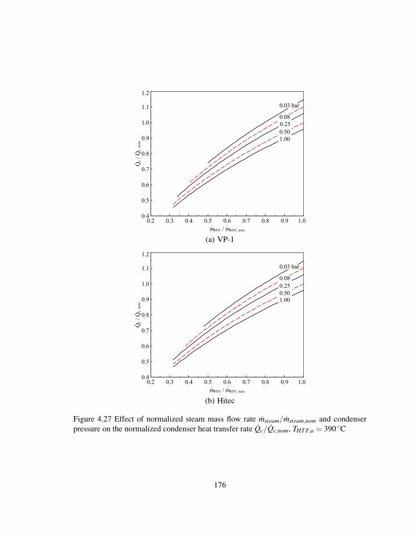
1.000.500.250.08

0.03 bar

Qc /

Qc,

nom

0.4

0.5

0.6

0.7

0.8

0.9

1.0

1.1

1.2

mHTF / mHTF, nom

0.2 0.3 0.4 0.5 0.6 0.7 0.8 0.9 1.0

(a) VP-1

1.000.500.250.08

0.03 bar

Qc /

Qc,

nom

0.4

0.5

0.6

0.7

0.8

0.9

1.0

1.1

1.2

mHTF / mHTF, nom

0.2 0.3 0.4 0.5 0.6 0.7 0.8 0.9 1.0

(b) Hitec

Figure 4.27 Effect of normalized steam mass flow rate msteam/msteam,nom and condenserpressure on the normalized condenser heat transfer rate Qc/Qc,nom, THT F,a = 390◦C

176

THTF,a = 390 oCTHTF,a = 350 oCTHTF,a = 310 oC

T HTF

, ret /

T HTF

, ret

, nom

0.6

0.7

0.8

0.9

1.0

mHTF / mHTF, nom

0.2 0.3 0.4 0.5 0.6 0.7 0.8 0.9 1.0

(a) VP-1

390 oC350 oC310 oC

T HTF

, ret /

T HTF

, ret

, nom

0.6

0.7

0.8

0.9

1.0

mHTF / mHTF, nom

0.2 0.3 0.4 0.5 0.6 0.7 0.8 0.9 1.0

(b) Hitec

Figure 4.28 Effect of normalized steam mass flow rate msteam/msteam,nom and condenserpressure on the return HTF temperature, Pc = 0.08 bar

177

The normalized input parameters are as follows:

m∗HT F =mHT F

mHT F,nomT ∗HT F,i =

THT F,i

THT F,i,nomP∗cond =

Pcond

Pcond,nom

and

Φ =Wnet

Wnet,nom,

Qc

Qc,nom,

THT F,ret

THT F,ret,nom

The regression model was written in Python 2.6 by using “leastsq” module, which is

a wrapper around MINPACK lmdif and lmder algorithms [102]. The input parameters

used for the power block simulation are described in Table 4.8. Tables 4.9 and 4.10 show

the coefficients obtained for the proposed linear regression. Values of the coefficient of

determination, R2, and root mean square error RMSE are also shown in Tables 4.9 and

4.10.

The results show that the linear regression accurately represents the behavior of the pa-

rameters (Wnet/Wnet,nom, Qc/Qc,nom, Tret,HT F/Tret,HT F,nom), obtained from the power block

model. This is corroborated by the Figure 4.29, which shows a comparison of the parame-

ters obtained from the linear regression with the power block model.

Table 4.8 Inputs parameters for the power block simulation

Inlet HTF Temperature, THT F,i (◦C) 290 - 390

Nominal Inlet HTF Temperature, THT F,i,nom (◦C) 390

Dimensionless HTF mass flow rate, mHT F/mHT F,nom 0.3 - 1.0

Condenser Pressure, Pcond (bar) 0.03 - 1 bar

Nominal condenser Pressure, Pcond,nom (bar) 0.08

Power Block 50 MWe

178

Table 4.9 Coefficients used for the proposed linear correlation given by Equation 4.159,HTF: VP-1

Coefficients Wnet/Wnet,nom Qc/Qc,nom Tret,HT F/Tret,HT F,nom

ψ0 -7.118 -4.473 -1.172

ψ1 8.864×10−2 -5.732×10−2 9.454×10−2

ψ2 -1.228×10−1 -8.135×10−2 -3.832×10−33

ψ3 10.957 6.579 1.836

ψ4 -3.839 -2.111 -6.643×10−1

ψ5 -2.202×10−1 4.075×10−2 7.979×10−4

ψ6 -1.477×10−2 2.196×10−3 5.431×10−5

ψ7 1.567×10−2 2.934×10−3 -4.768×10−6

ψ8 6.326×10−1 6.154×10−1 3.602×10−2

ψ9 1.532×10−1 8.269×10−3 -8.791×10−4

R2 0.9995 0.9999 0.9998

RMSE 0.0101 0.0035 0.0011

Table 4.10 Coefficients used for the proposed linear correlation given by Equation 4.159,HTF: Hitec

Coefficients Wnet/Wnet,nom Qc/Qc,nom Tret,HT F/Tret,HT F,nom

ψ0 -7.123 -4.485 -1.157

ψ1 1.798×10−2 -1.055×10−1 7.796×10−2

ψ2 -1.210×10−1 -7.624×10−2 -5.264×10−3

ψ3 11.185 6.754 1.847

ψ4 -4.063 -2.274 -6.911×10−1

ψ5 -2.056×10−1 3.859×10−2 8.678×10−4

ψ6 -1.492×10−2 2.294×10−3 5.863×10−5

ψ7 1.589×10−2 2.721×10−3 -2.678×10−7

ψ8 6.842×10−1 6.532×10−1 4.800×10−2

ψ9 1.385×10−1 1.023×10−2 -9.883×10−4

R2 0.9999 1.0000 0.9997

RMSE 0.0045 0.0014 0.0011

179

VP-1Hitec

Wne

t / W

net,

nom, L

inea

r Reg

ress

ion

0.0

0.1

0.2

0.3

0.4

0.5

0.6

0.7

0.8

0.9

1.01.1

Wnet / Wnet, nom, Model0.0 0.1 0.2 0.3 0.4 0.5 0.6 0.7 0.8 0.9 1.0 1.1

(a) Wnet/Wnet,nom

VP-1Hitec

Qc /

Qc,

nom

, Lin

ear R

egre

ssio

n

0.0

0.1

0.2

0.3

0.4

0.5

0.6

0.7

0.8

0.9

1.01.1

Qc / Qc, nom, Model0.0 0.1 0.2 0.3 0.4 0.5 0.6 0.7 0.8 0.9 1.0 1.1

(b) Qc/Qc,nom

Figure 4.29 Comparison of the dimensionless net work output and condenser heat transferrate obtained from the linear correlation with the proposed power block model, HTF: VP-1and Hitec

4.13 Conclusions

A comprehensive model for the simulation of a regenerative Rankine cycle was de-

veloped. The results obtained showed that the output power from the cycles is affected

mainly by: the inlet heat transfer fluid (HTF) temperature, mass flow rate of the HTF and

the condenser pressure. The cycle parameters were normalized and it was found that the

performance was independent of the power block size.

A linear regression was proposed by using the normalized variables, the results showed

that the linear equation represents accurately the trend given by the results obtained in the

simulation.

180

Chapter 5

Solar Field Piping and Thermal Losses

5.1 Solar Field Layout

The solar piping system circulates the heat transfer fluid (HTF) in a closed loop to

and from the power block and solar field. This system is designed to maintain an equally

distributed flow through all the solar collector loops and thus to avoid hot spots or cold

spots [140]. The solar piping model in this chapter is based on the model developed by

National Renewable Laboratory (NREL) [141]. In this model two layouts were proposed:

an H field layout for collectors areas greater than 400000 m2, and an I layout for areas less

than 400000 m2.

5.1.1 H Field Layout

As shown in Figure 5.1, in this layout the solar field is divided into 4 header pairs, with

the power block located at the center of the solar field. Cold fluid is distributed from the

cold header to each solar loop and returns to the hot header where it goes back to the power

block. Each collector loop consists of 6 LS-3 solar collectors which are arranged in series

to increase the temperature of the HTF to the operating conditions. In a solar collector

loop, the solar collectors are connected by ball joints, which are used to allow independent

rotation of the adjacent solar collectors [3].

181

POWER BLOCK

N

……

……

……

……

Cold Header

Hot Header

……

……

……

……

……

……

……

……

Cold Header

Hot Header

……

……

……

……

Collector Loop

LRow

LLoop=2

POWER BLOCK

110 m

Figure 5.1 H solar field layout. Adapted from [3]

182

The ball joints are preferred over flexible hoses due to their advantages which include:

lower cost, reduced pressure drop, and reduced heat losses [3]. In order to reduce the land

requirements and piping power, the collector loop has two rows such that the cold and hot

headers are located in the same side.

5.1.2 I Field Layout

In this layout the solar field is divided into a 2 header pairs, as shown in Figure 5.2,

with the power block located at the center of the solar field. Cold and hot header run East-

West direction. Each collector loop consists of 16 LS-2 solar collectors. As in H solar

field layout, the LS-2 collectors are arranged in series with two rows. The dimensions and

properties of LS-2 and LS-3 solar collectors are shown in Appendix B.

POWER BLOCK

N

……

……

……

……

Cold HeaderHot Header

……

……

Collector Loop

Cold HeaderHot Header

L R ow

L L oop =2

110 m

Figure 5.2 I solar field layout. Adapted from [3]

183

For both layouts, the maximum pressure drop is given by the longest path in the HTF

circuit. This pressure drop is calculated for the solar field and the power block (heat ex-

changers, internal piping, etc.).

5.2 Pressure Drop in the Solar Field

The pressure drop in the solar field depends on: the HTF, mass flow rate, inner diameter

of the pipes and fittings (elbow, cross, reduction, expansion, valves, etc.). Initially, it is

necessary to determine the optimum diameter for each section. The calculations are based

on the optimum flow velocity for minimizing of the piping costs given by NREL [141],

which is in the range of 2-4 m/s. A flow velocity of 2 m/s, also used in [16], was selected for

all the piping modeling. The pipe in each section must meet the flow conditions (optimum

velocity) and the pressure requirements. For the pressure requirements the required wall

thickness is calculated as [142]:

twall =(Pabs−Patm) Do

2 [Sy +0.4 (Pabs−Patm)](5.1)

where Pabs is the absolute pressure of HTF in psi, Patm is the atmospheric pressure in psi,

Dois the outside diameter in inches, and Sy is the allowable stress in psi. As recommended

by NREL [141], three different pipe materials are used:

• ASTM A106, Grade B, Seamless Carbon Steel pipe

• ASTM A335 P9, Intermediate Alloy Steel

• ASTM TP347, Stainless Steel

184

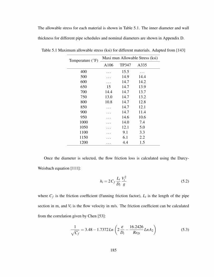
The allowable stress for each material is shown in Table 5.1. The inner diameter and wall

thickness for different pipe schedules and nominal diameters are shown in Appendix D.

Table 5.1 Maximum allowable stress (ksi) for different materials. Adapted from [143]

Temperature (◦F)Maxi mun Allowable Stress (ksi)

A106 TP347 A335

400 . . . 15.5 . . .500 . . . 14.9 14.4600 . . . 14.7 14.2650 15 14.7 13.9700 14.4 14.7 13.7750 13.0 14.7 13.2800 10.8 14.7 12.8850 . . . 14.7 12.1900 . . . 14.7 11.4950 . . . 14.6 10.6

1000 . . . 14.0 7.41050 . . . 12.1 5.01100 . . . 9.1 3.31150 . . . 6.1 2.21200 . . . 4.4 1.5

Once the diameter is selected, the flow friction loss is calculated using the Darcy-

Weisbach equation [111]:

hi = 2C fLi

Di

V 2ig

(5.2)

where C f is the friction coefficient (Fanning friction factor), Li is the length of the pipe

section in m, and Vi is the flow velocity in m/s. The friction coefficient can be calculated

from the correlation given by Chen [53]:

1√C f

= 3.48−1.7372Ln(

2ε

Di− 16.2426

ReDLnA2

)(5.3)

185

A2 =(2ε/Di)

1.1098

6.0983+

(7.149ReD

)0.8981

where ReD is the Reynolds number, ε is the pipe roughness in m. This correlation is valid

for 4000≤ ReD ≤ 108 and 2 × 10−8 ≤ ε/a≤ 0.1. For all the pipe materials it is assumed

that the pipe roughness has a value of ε = 0.046 mm [144]. The pressure drop in a section

is given by:

∆PLi = ρi g hi (5.4)

The friction losses through the pipe fittings are calculated as:

L f i = K[

Di

2C f

](5.5)

where L f i is the pipe length which gives the same pressure drop as the fitting. The pressure

drop through the fitting is:

h f i = 2C fL f i

Di

V 2ig

(5.6)

∆PL f i = ρi g h f i (5.7)

The K factors are given in Table 5.2. The location and number of fittings used was

set by the description given by NREL [141]. Table 5.3 and 5.4 summarize the types and

locations of the fittings used in each loop as well as the length of the cold and hot header.

As seen in Table 5.3 , expansion loops are every other loop to maintain pipe stresses within

the limits allowed [140].

186

Table 5.2 K values for different pipe fittings used in the solar field. Adapted from [141]

Fitting K

Gate Valve 0.19Globe Valve 10.00Check Valve 2.50Standard Elbow 0.90Medium Elbow 0.75Long Elbow 0.60Weldolet 1.80Ball Joint 4.73Flexible Hose 20.60

The pressure drop through the solar field is calculated for the longest path traveled by

the HTF. The pressure drop is then calculated as:

∆PSF = ∆PH +∆PC +∑i

∆Pi,loop,H +∑i

∆Pi,loop,C +∆Pin,out +∆Pcollector (5.8)

where ∆PH is the pressure drop in the outlet hot header, ∆PC is the pressure drop in the

inlet cold header, ∆Pi,loop,H is the pressure drop in the hot header pipe at the position of the

loop i, ∆Pi,loop,C is the pressure drop in the cold header pipe at the position of the loop i,

∆Pin,out is the pressure drop in the inlet and outlet of the solar collector loop, and ∆Pcollector

is the pressure drop in the solar collector loop. The pressure drop through the power block

should be included as well. Table 5.5 shows the typical length and fittings used in a power

block unit. The description of each line is as follows:

• Line 1: Expansion vessel or thermal storage tank to pump suction header

• Line 2: Individual pump suction line, from suction header to pump inlet

• Line 3: Individual pump discharge line, from pump discharge to discharge header

187

Table 5.3 Fittings used in the Heat Collection Element (HCE) loop. Adapted from [141]

Accessories and Pipe Inlet and Outlet HCE To Loopa To Loop From Loopa From Loop

Pipe Length (m)b LRow +40 LLoop = LHCE × nSCE 2 LRow +19 2 LRow 2 LRow +19 2 LRowStandard Elbows 2 10 0 0 0 0Medium Elbows 0 0 0 0 0 0Long Elbows 0 0 4 0 8 0Gate Valves 2 0 0 0 0 0Globe Valves 0 0 0 0 0 0Check Valves 0 0 0 0 0 0Loop Weldolets 2 0 0 0 0 0Loop Control Valves 1 0 0 0 0 0Ball Jointsc 0 2+nSCE 0 0 0 0

a Every other loopb LRow: Row spacing, LRow ≈ 12−15m [3]c nSCE : Number of solar collector assemblies, LS-2 nSCE = 16, LS-3 nSCE = 6 [3]

188

Table 5.4 Header length and fittings used in the solar field piping layout. Adapted from[143]

Cold Header Hot Header

Length (m)

Position of Power Block Configuration I Configuration H

Center 50 20+0.5 LLoopNorth-South 20+0.5 LRow 50+0.5 LLoopEast-West 50 20+0.5 LLoop

Accessories

Standard elbows 0 0Medium elbows 0 0Long elbows 8 8Gate valves 1 1Globe valves 0 0Check valves 1 0Loop Weldolets 0 0Loop control valves 0 0Ball Joints 0 0

• Line 4: Pump discharge header

• Line 5: Collector field outlet header to expansion vessel or thermal storage tank

• Line 6: Steam generator supply header

• Line 7: Inter steam generator piping

• Line 8: Steam generator exit header to expansion vessel or thermal storage

The total pressure drop in the power block is given by:

∆PPB =7

∑i=1

∆PLine,i +∆PHE (5.9)

189

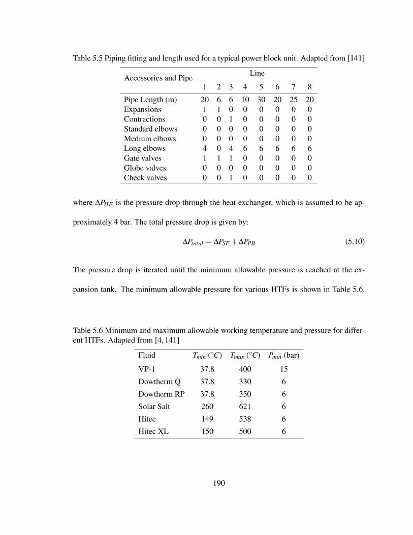
Table 5.5 Piping fitting and length used for a typical power block unit. Adapted from [141]

Accessories and PipeLine

1 2 3 4 5 6 7 8

Pipe Length (m) 20 6 6 10 30 20 25 20Expansions 1 1 0 0 0 0 0 0Contractions 0 0 1 0 0 0 0 0Standard elbows 0 0 0 0 0 0 0 0Medium elbows 0 0 0 0 0 0 0 0Long elbows 4 0 4 6 6 6 6 6Gate valves 1 1 1 0 0 0 0 0Globe valves 0 0 0 0 0 0 0 0Check valves 0 0 1 0 0 0 0 0

where ∆PHE is the pressure drop through the heat exchanger, which is assumed to be ap-

proximately 4 bar. The total pressure drop is given by:

∆Ptotal = ∆PSF +∆PPB (5.10)

The pressure drop is iterated until the minimum allowable pressure is reached at the ex-

pansion tank. The minimum allowable pressure for various HTFs is shown in Table 5.6.

Table 5.6 Minimum and maximum allowable working temperature and pressure for differ-ent HTFs. Adapted from [4, 141]

Fluid Tmin (◦C) Tmax (◦C) Pmin (bar)

VP-1 37.8 400 15

Dowtherm Q 37.8 330 6

Dowtherm RP 37.8 350 6

Solar Salt 260 621 6

Hitec 149 538 6

Hitec XL 150 500 6

190

The HTF is circulated in a closed loop by using a variable speed pump [140]. The pump

power is the highest parasitic load in the solar plant and therefore a variable speed pump is

used to reduce the power requirements when the solar field requires flow rates less than the

nominal rate. The pumping requirement is calculated as:

Wp,nom = ρHT F,Tcold g ∆Ptotal (5.11)

At different speeds, the pump law is used and the pump work is given by [145]:

Wp = Wp,nom

(mSF

mSF,nom

)3

(5.12)

where mSF is the current mass flow rate, and mSF,nom is the mass flow rate at nominal

condition. The pump efficiency is affected by the solar field mass flow rate as well:

ηp,SF

ηp,SF,nom= αo +2 (1−αo)

mSF

mSF,nom− (1−αo)

(mSF

mSF,nom

)2

(5.13)

with αo = −0.4 as recommended by Lippke [5]. The net electric power required by the

solar field pump is:

Wnet,pump = Wp/ηp,SF (5.14)

During night, the solar field operates at 20% of the nominal flow rate to keep the pipes

and solar collectors warm, and avoid thermal shock due to sudden temperature drops or

rises. When the temperature drops beyond the minimum allowable temperature, an external

heater systems is activated to avoid freezing problems.

191

5.3 Thermal Losses

Thermal losses take place in the solar field piping owing to the temperature difference

between the HTF and the surrounding air. The way to mitigate the thermal losses is by

adding insulation to the pipes, but adding too much insulation generates excessive cost

with little extra benefits. For this reason, an optimum thickness is calculated at nominal

conditions which minimizes the costs and thermal losses. In this chapter, the methodology

developed by Bahadori and Vuthaluru [146] is used. This methodology determines the op-

timum economic thickness of the thermal insulation as a function of the steel pipe diameter

and the surface temperature.

As a conservative assumption for insulated pipes, thermal resistances of the pipe walls

and the exterior air film are neglected [147]. This assumption simplifies the calculation of

thermal losses. The total thermal losses are given by:

Qpiping = 2π

kins,H (TH−Ta) ∑i

Li

ln(

Doi,pipe +2δins,i

Doi,pipe

)+

kins,C (TC−Ta) ∑j

L j

ln(

Do j,pipe +2δins, j

Do j,pipe

) (5.15)

where kins,H is the thermal conductivity of the pipe insulation evaluated at TH =(TH +Ta)/2,

kins,C is the thermal conductivity of the pipe insulation evaluated at TC = (TC +Ta)/2. The

above Equation can be rewritten as:

Qpiping = 2π[kins,H (TH−Ta) ζH + kins,C (TC−Ta) ζC

](5.16)

192

ζH = ∑i

Li

ln(

Doi,pipe +2δins,i

Doi,pipe

)

ζC = ∑j

L j

ln(

Do j,pipe +2δins, j

Do j,pipe

)The insulation thickness is a function of the steel outer pipe:

ln (δins) =3

∑n=0

αn D−no (5.17)

The coefficients αn are expressed as functions of the thermal conductivity as follows:

αn = An +Bn

kins+

Cn

k2ins

+Dn

k3ins

(5.18)

The following interpolation is used for the other surface temperatures:

δins = δins,T1 +(T −T1)(δins,T2−δins,T1)

(T2−T1)(5.19)

where δ1 and δ2 are calculated at T1 and T2 respectively. Due to the low thermal resistance

in the wall pipe, the surface temperature is assumed to be the HTF temperature. The thermal

conductivity of typical insulation material used in CSP plants is shown in Table 5.7 for

different temperatures. The coefficients, An, Bn, Cn and Dn are shown in Table 5.8.

Table 5.7 Thermal conductivity, in kW/m K, of pipe insulation materials. Data taken from[56, 148]

Temperature (◦C) Mineral Wool Temperature (◦C) Calcium Silicate

38 0.0336 36.9 0.05593 0.0432 91.9 0.059

149 0.0525 146.9 0.063204 0.0624 256.9 0.075260 0.0730 371.9 0.089316 0.0853 476.9 0.104371 0.0997 . . . . . .

193

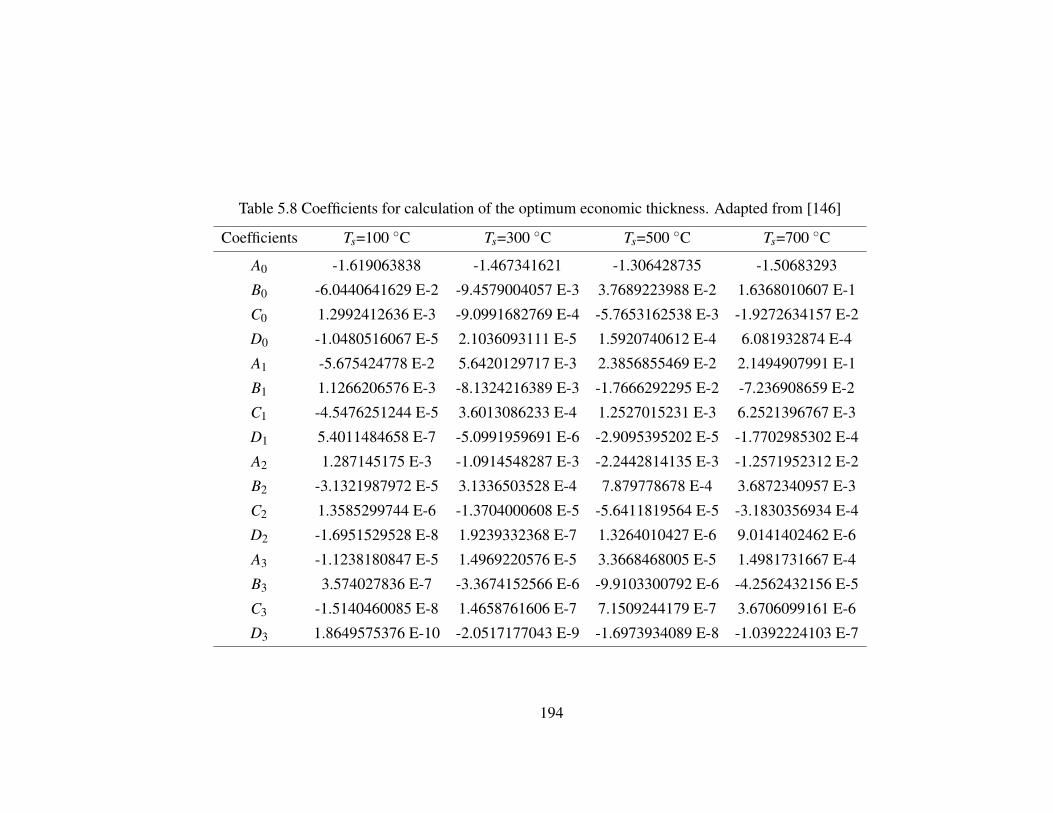
Table 5.8 Coefficients for calculation of the optimum economic thickness. Adapted from [146]

Coefficients Ts=100 ◦C Ts=300 ◦C Ts=500 ◦C Ts=700 ◦C

A0 -1.619063838 -1.467341621 -1.306428735 -1.50683293

B0 -6.0440641629 E-2 -9.4579004057 E-3 3.7689223988 E-2 1.6368010607 E-1

C0 1.2992412636 E-3 -9.0991682769 E-4 -5.7653162538 E-3 -1.9272634157 E-2

D0 -1.0480516067 E-5 2.1036093111 E-5 1.5920740612 E-4 6.081932874 E-4

A1 -5.675424778 E-2 5.6420129717 E-3 2.3856855469 E-2 2.1494907991 E-1

B1 1.1266206576 E-3 -8.1324216389 E-3 -1.7666292295 E-2 -7.236908659 E-2

C1 -4.5476251244 E-5 3.6013086233 E-4 1.2527015231 E-3 6.2521396767 E-3

D1 5.4011484658 E-7 -5.0991959691 E-6 -2.9095395202 E-5 -1.7702985302 E-4

A2 1.287145175 E-3 -1.0914548287 E-3 -2.2442814135 E-3 -1.2571952312 E-2

B2 -3.1321987972 E-5 3.1336503528 E-4 7.879778678 E-4 3.6872340957 E-3

C2 1.3585299744 E-6 -1.3704000608 E-5 -5.6411819564 E-5 -3.1830356934 E-4

D2 -1.6951529528 E-8 1.9239332368 E-7 1.3264010427 E-6 9.0141402462 E-6

A3 -1.1238180847 E-5 1.4969220576 E-5 3.3668468005 E-5 1.4981731667 E-4

B3 3.574027836 E-7 -3.3674152566 E-6 -9.9103300792 E-6 -4.2562432156 E-5

C3 -1.5140460085 E-8 1.4658761606 E-7 7.1509244179 E-7 3.6706099161 E-6

D3 1.8649575376 E-10 -2.0517177043 E-9 -1.6973934089 E-8 -1.0392224103 E-7

194

5.4 Expansion Tank

The expansion tank provides space for expansion of the HTF due to the change in

volume when the HTF is heated up in the solar field to the operating temperature. The

expansion tank is usually installed at the highest point in the solar field next to the pump.

This tank is used to vent the moisture that accumulates in the HTF and to create positive

head pressure to the pump inlet as well.

The expansion tank should be sized so that it is 25% full at ambient temperature and

75% full at the normal operating temperature [149]. Usually the expansion tank is blan-

keted with nitrogen to maintain a non-reactive atmosphere and keeping a positive pressure

which prevents air and moisture from entering the tank [149]. The heat transfer losses

from the tank to the surrounding air are significant and should be taken into account along

with the thermal piping losses to calculate the total thermal losses in the solar field. The

increment in the HTF volume is given by:

∆VHT F =

(ρTre f

ρTC

−1) (

Vc +14

Vexp,tank Ntank

)+

(ρTre f

ρTH

−1)(VH +Vcollectors

+Vin,out)+

(ρTre f

ρTH

−1)

VH (5.20)

Vc =π

4 ∑i

D2innner,iLi (5.21)

VH =π

4 ∑j

D2innner, jL j (5.22)

Vcollector =π

4nloops D2

receiverLc (5.23)

195

where ρTre f is the density of the HTF calculated at reference condition, 25 ◦C, ρTC is the

density of the HTF calculated at cold temperature, ρTH is the density of the HTF calculated

at hot temperature, Vc is the total volume of the cold header, Vin,out is the total volume of

the inlet and outlet pipe of the collector loop, and Vc is the total volume of solar receiver.

For the solar field, multiple expansion tanks with a volume of 283 m3 [140] were

selected. The dimensions of this tank are approximately: Dtank = 6m and Htank = 10 m.

The number of tanks is calculated as:

Ntank =

∆VHT F/

12

Vexp,tank if mod(

∆VHT F ,12

Vexp,tank

)= 0

int(

∆VHT F/12

Vexp,tank

)+1 if mod

(∆VHT F ,

12

Vexp,tank

)6= 0

(5.24)

The procedure for heat losses in the expansion tank was taken from the methodology

developed by Kumana and Kothari [150]. For the heat loss calculation in the expansion

tank it is assumed that:

• Fouling factors are negligible

• Radiation losses are negligible

• Temperature in the gas and liquid sections is uniform

• Thermal equilibrium exists between the gas and the liquid fluid

As shown in Figure 5.3, the four individual losses in the tank need to be calculated.

The heat loss from each surface is shown below. For dry sidewall:

Qd =Ud Ad (Tgas−T∞) (5.25)

196

ttw

tI

Di;t

_Qb

_Qw

_Qd

_Qr

Lw

L

Tank wall

Insulation

Gas

Liquid

Figure 5.3 Thermal losses from a vertical tank. Adapted from [150]

Ud =

[1

h∞,d+DI

ln (DI/Do,t)

2kI+DI

ln (Do,t/Di,t)

2ktw+

1hgas,d

(DI

Di,t

)]−1

(5.26)

Ad = π DI (L−Lw) (5.27)

DI = Di,t +2 ttw +2 tI (5.28)

For wet sidewall:

Qw =UW AWw(TLiquid−T∞

)(5.29)

Uw =

[1

h∞,w+DI

ln (DI/Do,t)

2kI+DI

ln (Do,t/Di,t)

2ktw+

1hLiquid,w

(DI

Di,t

)]−1

(5.30)

Aw = π DI Lw (5.31)

For tank bottom:

Qb =Ub Ab(TLiquid−T∞

)(5.32)

197

Ub =

[1

h∞,b+

tIkI

+ttwktw

+1

hLiquid,b

]−1

(5.33)

Ab = π D2i,t/4 (5.34)

For tank roof:

Qr =Ur Ar (TGas−T∞) (5.35)

Ur =

[1

h∞,r+

tIkI

+ttwktw

+1

hgas,r

]−1

(5.36)

Ar = π D2i,t/4 (5.37)

Therefore, the total heat losses are:

Qtank,losses = Qd + Qw + Qb + Qr (5.38)

The convective heat transfer coefficients are detailed below. h∞,d and h∞,w are calcu-

lated for two cases: wind or no wind condition. For the wind condition a cylinder in cross

flow is used. The average Nusselt number recommended for a cylinder in cross flow [53]

is given by:

NuD = cRemD Prn

(Pr

Prw

)p

(5.39)

h∞,d =NuD kair

DI(5.40)

h∞,w =NuD kair

DI(5.41)

The constants suggested for this equation are tabulated in Table 3.8. The value of p depends

on the heat flux direction: p = 0.25 for fluid heating and p = 0.2 for fluid cooling. For no

198

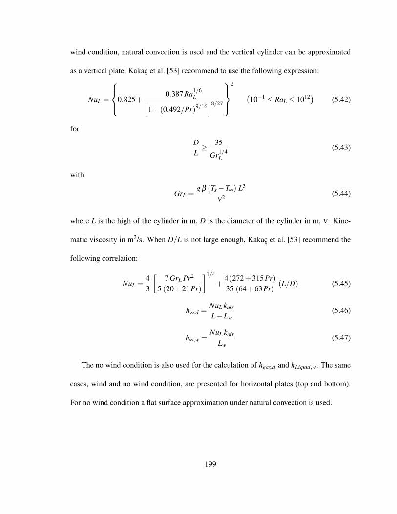
wind condition, natural convection is used and the vertical cylinder can be approximated

as a vertical plate, Kakaç et al. [53] recommend to use the following expression:

NuL =

0.825+0.387 Ra1/6

L[1+(0.492/Pr)9/16

]8/27

2 (

10−1 ≤ RaL ≤ 1012) (5.42)

for

DL≥ 35

Gr1/4L

(5.43)

with

GrL =g β (Ts−T∞) L3

ν2 (5.44)

where L is the high of the cylinder in m, D is the diameter of the cylinder in m, ν : Kine-

matic viscosity in m2/s. When D/L is not large enough, Kakaç et al. [53] recommend the

following correlation:

NuL =43

[7 GrL Pr2

5 (20+21Pr)

]1/4

+4(272+315 Pr)35 (64+63Pr)

(L/D) (5.45)

h∞,d =NuL kair

L−Lw(5.46)

h∞,w =NuL kair

Lw(5.47)

The no wind condition is also used for the calculation of hgas,d and hLiquid,w. The same

cases, wind and no wind condition, are presented for horizontal plates (top and bottom).

For no wind condition a flat surface approximation under natural convection is used.

199

Natural convection , upper surface of hot plate or lower surface of cold plate (h∞,r,

hgas,r) [111]:

NuLD = 0.54 Ra1/4L

(104 ≤ RaL ≤ 107) (5.48)

NuLD = 0.15 Ra1/4L

(107 ≤ RaL ≤ 1011) (5.49)

Natural convection, lower surface of hot plate or upper surface of cold plate (h∞,b,

hLiquid,r) [111]:

NuLD = 0.27 Ra1/4L

(105 ≤ RaL ≤ 1010) (5.50)

with

LD =As

P=

Di,t

4(5.51)

RaLD =g β (Ts−T∞) L3

Dν α

(5.52)

h =NuLD k

LD(5.53)

where As and P are the plate surface area and perimeter, respectively. For wind condition

(h∞,b and h∞,r), the wind enhancement factor ζw is calculated as [150]:

ζw =h∞,w|wind

h∞,w|no,wind(5.54)

and

h∞,b∣∣wind = ζw

(h∞,b

∣∣no wind

)(5.55)

h∞,r|wind = ζw(

h∞,r|no wind

)(5.56)

200

In order to calculate the heat transfer coefficients, it is necessary to obtain the wall

temperatures which require an iterative procedure. The total heat losses are calculated as:

Qtotal,tank = Qtank,losses, f ull Ntank, f ull + Qtank,losses,partial

+Qtank,losses,empty Ntank,empty (5.57)

where Qtank,losses, f ull Ntank, f ull is the total heat losses for the tanks completely filled

(0.75 Vexp,tank), Qtank,losses,partial is the total heat losses for the tank partially filled

(V < 0.75 Vexp,tank), and Qtank,losses,empty Ntank,empty is the total heat losses for the tanks

filled at nominal conditions (0.25Vexp,tank).

5.5 Conclusions

A comprehensive model for the pressure drop and pumping power requirement of a

solar field was performed. The model calculates the diameter and pressure drop in each

header section based on the pipe stress calculation and HTF flow rate distribution.

A heat losses model was also carried out for the piping system and the expansion tank.

The model calculates the thermal losses of the solar field piping for the optimum economic

thickness of the thermal insulation in each header section. For the expansion tank, the

thermal losses are calculated individually for the gas and liquid sections.

201

Chapter 6

Integration of System Components

In the previous chapters the different subsystems of the PTC solar power plant were

designed for nominal and partial conditions. In the final step, the subsystems must be

integrated into the plant and work together. For example, the energy coming from the solar

field runs the power block, the power block is affected by the ambient conditions and at the

same time the return HTF temperature from the power block affects the output from the

solar field. This kind of connection between the subsystems of the solar power plant affect

its performance under steady and transient conditions. Initially a preliminary design under

steady state conditions is performed, in the following steps:

• Calculation of Direct Normal Radiation (DNI).

• Calculation of the DNI cumulative frequency distribution (CFD), at this step a DNI

with 95 % of the cumulative frequency is selected as the reference radiation for the

preliminary design.

• Power block design:

– HTF selection.

– Conditions of operation of the power block (low pressure, high pressure, turbine

efficiency,etc).

202

– Temperature drop and mass flow rate of the HTF.

– Calculation of the parasitic losses in the condenser system.

• Selection of the solar collector.

• Solar collector performance under reference conditions: mass flow rate at nominal

conditions and the heat gained.

• Selection of solar field layout and determination of the number of loops.

• Calculation of the maximum pressure drop through the solar field.

• Calculation of pumping power requirement and heat losses.

• Calculation of the expansion tank volume and heat losses.

• Hourly simulation.

• Calculation of the optimum size by LCOE and solar energy utilization .

Figure 6.1 shows a flowchart of the different steps described above.

6.1 Transient Analysis

Although it is commonly assumed that the solar power plant operates under steady

state conditions, this assumptions is not true for most of the operation time. In this case, a

transient analysis is necessary to incorporate the thermal inertia of the system. The transient

energy balance of a Solar Collector Assembly (SCA) is given by [151] (Figure 6.2):

ddt

(mcollector CHT F T ) = mHT F CHT F (Tin−T )+ Qu (6.1)

203

References conditions

IDNI ; Tair;ref ; Vwind

Power BlockDesign

Condenser_Qcond; Pcond

_Wpar;cond

_mHTF

THTF ; oHTF; THTF;i

_mHTF;loopnloops

Solar Collector

Solar Field Layout

¢ PSF

_Wpump:SF_Qpiping;loss

+

_Wpar;total

-

_Wnet;cycle

_Wnet;SF

¢VSF

_Qexp;tank +

_Qtotal;losses

Cond: CondenserExp: ExpansionHTF: Heat Transfer FluidPar: ParasiticSF: Solar field

Figure 6.1 Logic flow for the preliminary design of the PTC solar plants

204

ii¡ 1 i + 1

_mHTF

_Qu;i¡1_Qu;i

_Qu;i+1

SCA SCA SCA

Figure 6.2 Node analysis of the solar collector assembly (SCA)

Integrating the last expression, it is obtained that:∫t1+∆t

t10

dTT −Tin− Qu/mHT F CHT F

=− mHT F

mcollector

∫t1+∆t

t10

dt (6.2)

T (t1 +∆t1) =

(T (t1)−THT F,in−

Qu

mHT F CHT F

)exp

(− mHT F

mcollector∆t)

+THT F,in +Qu

mHT F CHT F(6.3)

Using a nodal notation, the last expression can be rewritten as:

T n+1i =

(T n

i −T ni−1−

Qu,i

mHT F CHT F,i

)exp

(− mHT F

VSCA ρi∆t)

(6.4)

+T ni−1 +

Qu,i

mHT F CHT F,i(6.5)

VSCA =π

4D2

abs Lc

where T n+1i is the temperature at node i in the next time step.

The same transient analysis is employed for the the pipe header, after applying the

energy balance to the system (Figure 6.3) the next ordinary differential equation (ODE) is

found:

ddt

(mT CT T ) = m f CHT F (Tin−T )− Qloss (6.6)

205

_mf ; Tin _mf ; T

T; V

_Qloss = ³ (T ¡ Ta)

Figure 6.3 Thermal capacitance analysis of the pipe header

Qloss = ζ (T −Ta)

Integrating: ∫t1+∆t

t10

dTT −Tp

=−m f CHT F +ζ

mT CT

∫t1+∆t

t10

dt (6.7)

Tp =m f CHT F Tin +ζ Ta

m f CHT F +ζ

T (t1 +∆t1) = Tp +(T (t1)−Tp) exp(−

m f CHT F +ζ

mT CT∆t)

(6.8)

which may be rewritten as:

T n+1 = Tp +(T n−Tp) exp(−

m f CHT F +ζ

mT CT∆t)

(6.9)

The last Equation can be used for the thermal capacitance calculation of the hot header,

cold heater and expansion tank. The term mT CT includes the thermal capacitance of the

HTF, pipe walls and insulation. In this simulation, the thermal capacitance of the pipe

walls and insulation was distributed uniformly over the solar field. The same assumption

was used for the HTF in the hot and cold headers. Figures 6.4 and 6.5 show the distribution

206

......

......

......

Power Block

1

2VC

1

2VC

1

2VH

1

2VH

1

2Vcollector

1

2Vcollector

Ntank Vexp;tank

Figure 6.4 Thermal inertia distribution for I layout

......

......

......

Power Block

1

4VC

1

4VC

1

4VH

1

4VH

1

4Vcollector

Ntank Vexp;tank

1

4Vcollector

1

4VH

1

4VH

1

4VC

1

4VC

1

4Vcollector

1

4Vcollector

Figure 6.5 Thermal inertia distribution for H layout

207

Solar Field

IDNI(t) Tair(t) Vwind(t)

_mHTF;SF

_Qu;SFH

Power Block

THTF;o

_Wnet;cycle

_Wpump:SF

_Qcond

Condenser Unit

Tair(t) RH(t)

Pcond

_Wpar;cond

+-

-

_Wnet;SF

_Qtotal;losses

T nSF

T n+1SF

Yes

NO

t > tmax

t = t + ¢t

END

Figure 6.6 Logic flow used for the dynamic simulation of the PTC solar power plant

208

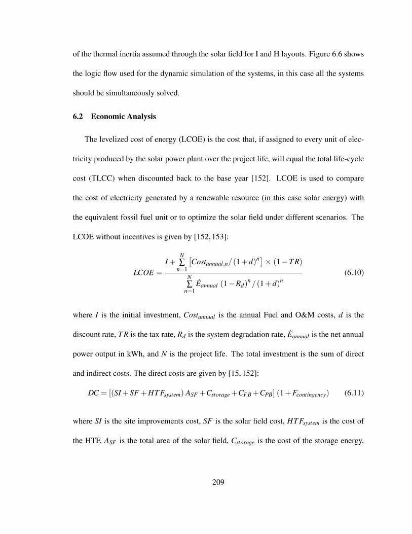
of the thermal inertia assumed through the solar field for I and H layouts. Figure 6.6 shows

the logic flow used for the dynamic simulation of the systems, in this case all the systems

should be simultaneously solved.

6.2 Economic Analysis

The levelized cost of energy (LCOE) is the cost that, if assigned to every unit of elec-

tricity produced by the solar power plant over the project life, will equal the total life-cycle

cost (TLCC) when discounted back to the base year [152]. LCOE is used to compare

the cost of electricity generated by a renewable resource (in this case solar energy) with

the equivalent fossil fuel unit or to optimize the solar field under different scenarios. The

LCOE without incentives is given by [152, 153]:

LCOE =

I +N∑

n=1

[Costannual,n/(1+d)n] × (1−T R)

N∑

n=1Eannual (1−Rd)

n /(1+d)n(6.10)

where I is the initial investment, Costannual is the annual Fuel and O&M costs, d is the

discount rate, T R is the tax rate, Rd is the system degradation rate, Eannual is the net annual

power output in kWh, and N is the project life. The total investment is the sum of direct

and indirect costs. The direct costs are given by [15, 152]:

DC = [(SI +SF +HT Fsystem) ASF +Cstorage +CFB +CPB] (1+Fcontingency) (6.11)

where SI is the site improvements cost, SF is the solar field cost, HT Fsystem is the cost of

the HTF, ASF is the total area of the solar field, Cstorage is the cost of the storage energy,

209

CFB is the cost of fossil back up, CPB is the cost of the power block, and Fcontingency is the

contingency factor. The indirect costs are as follows:

IC = DC (EPC+PLM+ST ) (6.12)

where EPC is the engineer, procure and construct cost, PLM is the project, land and man-

agement cost, and ST is the sale Tax. The annual costs are calculated as:

Costannual = FC+FCC Pnom +VCG Eannual (MWh)+CFuel (6.13)

where FC is the fixed annual Cost, FCC is the fixed cost by capacity, VCG is the variable

cost per generation, and CFuelis the fuel cost. Table 6.1 shows the values assumed for the

economic analysis. The discount rate is used for the calculation of the present value by

taking into account the time value. Two different analyses can be performed by accounting

for the inflation: nominal discount rate (include inflationary effects), and real discount rate

(exclude inflationary effects). Discount rate can be converted from real to nominal and vice

versa by using the following formulas [152]:

dn = (1+dr) (1+ e)−1

dr = [(1+dr)/(1+ e)]−1 (6.14)

where dn is the nominal discount rate, dr is the real discount rate, and e is the inflation rate.

On the other hand, the effective tax rate, or combined state and federal tax rate is calculated

as [152]:

T R = ST R+FT R (1−ST R) (6.15)

where ST R is the state tax rate, and FT R is the federal tax rate.

210

Table 6.1 Costs, taxes and discount rate assumed for the economical analysis. Values takenfrom [15, 140, 152]

Direct Cost Value Units

Site Improvements 25 $/m2

Solar Field 295 $/m2

HTF System 90 $/m2

Storage 80 $/kWht

Fossil Backup 0 $/kW

Power Block (Wet-Cooled) 940 $/kW

Power Block (Dry-Cooled) 1160 $/kW

Contingency 10 % DC

Indirect Cost

Engineer, Procure and Construct 15 %DC

Project, Land and Management 3.5 %DC

Sales Tax 7.75 % DC

O&M Cost

Fixed Annual Cost 0 $/yr

Fixed Cost by Capacity 70 $/kW-yr

Variable Cost per Generation 3 $/MWh

Fuel Cost 0 $/MWh

Taxes, Interest and System Degradation

Real Discount Rate 8 %

Inflation Rate 2.5 %

Federal Tax Rate 35 %

State Tax Rate 8 %

Annual Degradation Rate 0.5 %

Project Life 30 years

211

6.3 Results

The solar power plant was simulated every hour by using the monthly average values.

Table 6.2 shows the parameters used for the hourly simulation. The solar field size was

increased by adding even collector loops to the solar layout, and a parametric analysis was

then carried out to get the optimum size.

Table 6.2 Parameter used for the hourly simulation

Nominal Power Output 50 MWe

Hours of Thermal Storage (TES): 0

Solar Radiation Data: TMY3

Location: Tampa, Daggett

HTF: VP1

Solar Collector: LS-3

Solar Receiver: UVACAnnulus under vacuum, P = 10−4

Torr

Layout: H

ηSF,pump [5]: 60%

mSF,night [141]: 20%

mSF,day,min: 20%

Condenser: Cooling TowerAir Cooled Condenser

The results obtained for the cooling tower used as the cooling system for the power

block are presented in Tables 6.3 and 6.4. As it was expected, there is a minimum LCOE

which corresponds to the optimum solar plant size. For Tampa this number corresponds

to 136 collector loops, while for Daggett the optimum LCOE corresponds to 88 collector

loops. The difference in the optimum number of loops is related to the solar radiation

distribution.

212

Table 6.3 Results obtained for Tampa. Parameters used for the simulation are given in Table 6.2

ASF (m2) nloops Wnet,cycle(kW) Wpar(kW) CFactor( %) LCOER (¢/kWh) LCOEN(¢/kWh) Net Power (GWh)

246343.6 72 49312.8 2344.4 14.3 37.3 45.9 59.0

273715.2 80 49312.8 2532.2 16.3 35.1 43.2 66.8

301086.7 88 49312.8 2678.4 18.2 33.4 41.1 74.7

328458.2 96 49312.8 2863.4 20.3 32.0 39.4 82.6

355829.7 104 49312.8 3020.6 22.1 31.1 38.4 89.7

383201.2 112 49312.8 3202.7 23.8 30.4 37.6 96.4

410572.8 120 49312.8 3367.1 25.5 29.9 37.0 102.8

437944.3 128 49312.8 3555.7 27.1 29.7 36.7 108.8

465315.8 136 49312.8 3760.6 28.5 29.6 36.7 113.8

492687.3 144 49312.8 3899.6 29.6 29.8 36.8 118.2

520058.8 152 49312.8 4112.1 30.8 30.0 37.1 122.3

547430.4 160 49312.8 4294.4 31.8 30.3 37.6 125.7

213

Table 6.4 Results obtained for Daggett. Parameters used for the simulation are given in Table 6.2

ASF (m2) nloops Wnet,cycle(kW) Wpar(kW) CFactor( %) LCOER (¢/kWh) LCOEN(¢/kWh) Net Power (GWh)

191600.6 56 49312.8 2481.3 18.8 24.8 30.3 77.1

218972.2 64 49312.8 2762.6 22.3 22.6 27.7 90.9

246343.7 72 49312.8 3053.1 25.6 21.3 26.1 103.6

273715.2 80 49312.8 3321.5 28.2 20.8 25.6 113.4

301086.7 88 49312.8 3619.3 30.2 20.7 25.5 120.7

328458.2 96 49312.8 3891.9 31.4 21.2 26.1 124.9

355829.8 104 49312.8 4197.1 32.7 21.6 26.7 129.0

383201.3 112 49312.8 4468.3 33.9 22.1 27.2 133.1

410572.8 120 49312.8 4766.8 34.9 22.6 28.0 136.2

437944.3 128 49312.8 5047.6 35.7 23.3 28.9 138.3

465315.8 136 49312.8 5360.0 36.2 24.2 29.9 139.5

214

Freq

uenc

y (%

)

0

2

4

6

8

10

12

DNI (kW/m2)0 0.1 0.2 0.3 0.4 0.5 0.6 0.7 0.8 0.9 1

(a) Tampa

Freq

uenc

y (%

)

0

2

4

6

8

10

12

DNI (kW/m2)0 0.1 0.2 0.3 0.4 0.5 0.6 0.7 0.8 0.9 1

(b) Daggett

Figure 6.7 Frequency distribution of Direct Normal Irradiance (DNI)

As seen in Figure 6.7, the frequency distribution of Direct Normal Irradiance (DNI)

for Tampa shows that its DNI is below 500 W/m2 for almost 27% of the year the while

for Daggett it is only for 15.8 % of the year. This implies that , for Tampa, in order to

increase the annual output from the solar field an appreciable increase in the solar field size

is required to compensate for those months when the solar radiation is low. For the case

of Daggett, higher radiation is obtained during the whole year and therefore the solar field

size is smaller as compared with Tampa. This is evidenced by Figure 6.8, which shows that

for Daggett a more uniform monthly average net power output is obtained as compared to

Tampa.

In order to validate the results obtained from the proposed model, it was compared

with a model developed by NREL, the Solar Advisor Model (SAM) [15]. Figures 6.9

and 6.10 show the results obtained, levelized cost of electricity evaluated at real discount

rate (LCOER), and the annual net power output, for Tampa and Daggett respectively. The

215

(a) Tampa (b) Daggett

Figure 6.8 Monthly average distribution of the net power output calculated at minimumLCOER. Parameters used for the simulation are given in Table 6.2

results show that the proposed model follows the trend given by SAM, but there are some

discrepancies. The assumptions and modeling of the physical phenomena are different

in both of these models, hence it is expected that the results obtained would have some

Proposed ModelSAM

LCO

E R ¢

/kW

h

20

25

30

35

40

Number of Loops70 80 90 100 110 120 130 140 150 160 170

(a) LCOER

Proposed ModelSAM

Net

Pow

er (M

Wh)

50

60

70

80

90

100

110

120

130

Number of Loops70 80 90 100 110 120 130 140 150 160 170

(b) Annual Net Power Output

Figure 6.9 Comparison of the LCOER and annual net power output between the proposedmodel and System Advisor Model (SAM) [15], location: Tampa. Parameters used for thesimulation are given in Table 6.2

216

Proposed ModelSAM

LCO

E R ¢

/kW

h

10

15

20

25

30

Number of Loops50 60 70 80 90 100 110 120 130 140

(a) LCOER

Proposed ModelSAM

Net

Pow

er (M

Wh)

0

20

40

60

80

100

120

140

160

180

Number of Loops50 60 70 80 90 100 110 120 130 140

(b) Annual Net Power Output

Figure 6.10 Comparison of the LCOER and annual net power output between the proposedmodel and System Advisor Model (SAM) [15], location: Daggett. Parameters used for thesimulation are given in Table 6.2

differences. As it was explained in chapter 3, the proposed model is more conservative

than the models developed by NREL, which explains why the net power output obtained

from the model is lower than the results obtained by SAM in both cities. The LCOER

calculated from the proposed model is also lower than the values obtained from SAM due

to the difference in the annual cost which is proportional to the annual net power output.

Another important parameter for the design of the PTC solar power plant is the utiliza-

tion of solar energy which is a measure of how much of the collected solar energy is used

by the power block [12]. The utilization is defined as:

Utilization =(Collected-Dissipated)Solar energy

CollectedSolar energy(6.16)

217

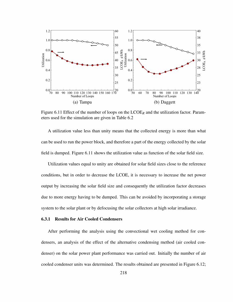
LCO

E R ¢

/kW

h

20

25

30

35

40

45

50

55

60

Util

izat

ion

0.0

0.2

0.4

0.6

0.8

1.0

1.2

Number of Loops70 80 90 100 110 120 130 140 150 160 170

(a) Tampa

LCO

E R ¢

/kW

h

20

23

25

28

30

33

35

38

40

Util

izat

ion

0.0

0.2

0.4

0.6

0.8

1.0

1.2

Number of Loops50 60 70 80 90 100 110 120 130 140

(b) Daggett

Figure 6.11 Effect of the number of loops on the LCOER and the utilization factor. Param-eters used for the simulation are given in Table 6.2

A utilization value less than unity means that the collected energy is more than what

can be used to run the power block, and therefore a part of the energy collected by the solar

field is dumped. Figure 6.11 shows the utilization value as function of the solar field size.

Utilization values equal to unity are obtained for solar field sizes close to the reference

conditions, but in order to decrease the LCOE, it is necessary to increase the net power

output by increasing the solar field size and consequently the utilization factor decreases

due to more energy having to be dumped. This can be avoided by incorporating a storage

system to the solar plant or by defocusing the solar collectors at high solar irradiance.

6.3.1 Results for Air Cooled Condensers

After performing the analysis using the convectional wet cooling method for con-

densers, an analysis of the effect of the alternative condensing method (air cooled con-

denser) on the solar power plant performance was carried out. Initially the number of air

cooled condenser units was determined. The results obtained are presented in Figure 6.12;

218

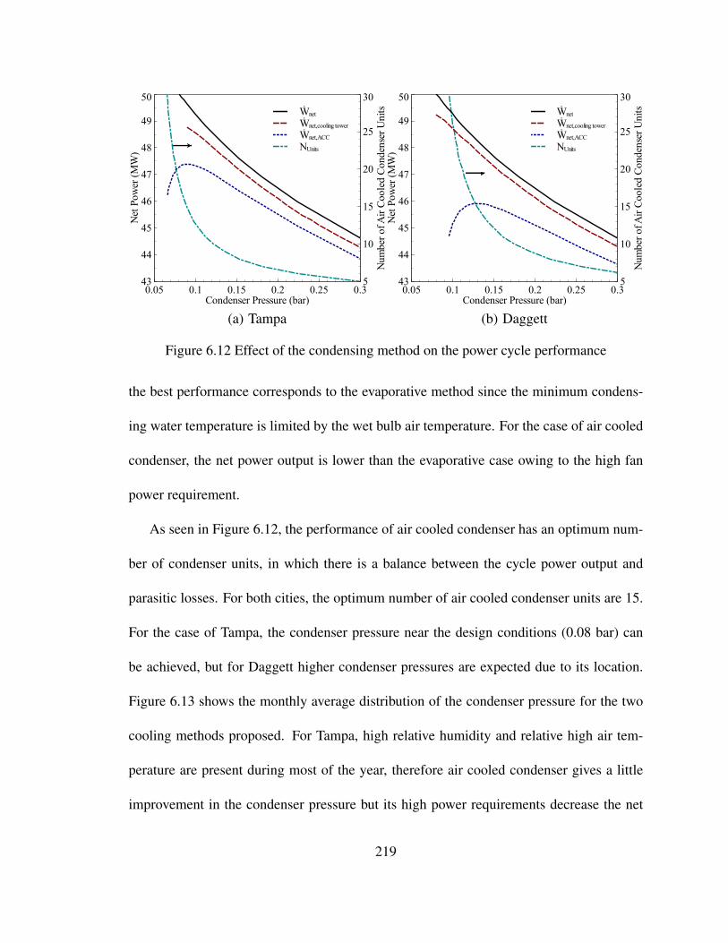
Num

ber o

f Air

Cool

ed C

onde

nser

Uni

ts

5

10

15

20

25

30WnetWnet,cooling towerWnet,ACCNUnits

Net

Pow

er (M

W)

43

44

45

46

47

48

49

50

Condenser Pressure (bar)0.05 0.1 0.15 0.2 0.25 0.3

(a) Tampa

Num

ber o

f Air

Cool

ed C

onde

nser

Uni

ts

5

10

15

20

25

30WnetWnet,cooling towerWnet,ACCNUnits

Net

Pow

er (M

W)

43

44

45

46

47

48

49

50

Condenser Pressure (bar)0.05 0.1 0.15 0.2 0.25 0.3

(b) Daggett

Figure 6.12 Effect of the condensing method on the power cycle performance

the best performance corresponds to the evaporative method since the minimum condens-

ing water temperature is limited by the wet bulb air temperature. For the case of air cooled

condenser, the net power output is lower than the evaporative case owing to the high fan

power requirement.

As seen in Figure 6.12, the performance of air cooled condenser has an optimum num-

ber of condenser units, in which there is a balance between the cycle power output and

parasitic losses. For both cities, the optimum number of air cooled condenser units are 15.

For the case of Tampa, the condenser pressure near the design conditions (0.08 bar) can

be achieved, but for Daggett higher condenser pressures are expected due to its location.

Figure 6.13 shows the monthly average distribution of the condenser pressure for the two

cooling methods proposed. For Tampa, high relative humidity and relative high air tem-

perature are present during most of the year, therefore air cooled condenser gives a little

improvement in the condenser pressure but its high power requirements decrease the net

219

Cooling Tower Air Cooled Condenser(a) Tampa

Cooling Tower Air Cooled Condenser(b) Daggett

Figure 6.13 Monthly average distribution of the condenser pressure. Parameter used for thesimulation are given in Table 6.2

220

power output. The opposite is seen in Daggett, where low relative humidity and conse-

quently low wet bulb temperature are present; for this location evaporative cooling method

provides acceptable condensing pressures to the power block. For Daggett, the air cooled

condensers generate a decrease in the cycle performance due to the higher condensing pres-

sures and higher parasitic losses due to the high air temperatures.

The evaluation of the air cooled condenser was performed for the solar field size corre-

sponding to the minimum LCOE. Table 6.5 shows the results obtained for evaporative and

air cooled condenser.

Table 6.5 Effect of the condenser type on the annual performance of the PTC solar powerplant. Parameters used for the simulation are given in Table 6.2

Wnet,cycle(kW) Wpar(kW) LCOER (¢/kWh) LCOEN(¢/kWh) Net Power (GWh)

Tampa, Cooling Tower

49312.8 3760.6 29.6 36.7 113.8

Tampa, Air Cooled Condenser

49312.8 5088.9 31.9 39.5 110.7

Daggett, Cooling Tower

49312.8 3619.3 20.7 25.5 120.7

Daggett, Air Cooled Condenser

49312.8 5363.3 22.8 28.1 116.2

The monthly performance of the PTC solar plant is shown in Figure 6.14. As it was

mentioned before, the fan power requirements and the high air temperatures decrease the

net power output, the difference is remarkable during summer days.

221

Cooling TowerAir Cooled Condenser

Mon

thly

Net

Pow

er (G

Wh)

0

2

4

6

8

10

12

14

16

1820

Jan Feb Mar Apr May Jun Jul Aug Sep Oct Nov Dec

(a) Tampa

Cooling TowerAir Cooled Condenser

Mon

thly

Net

Pow

er (G

Wh)

0

2

4

6

8

10

12

14

16

1820

Jan Feb Mar Apr May Jun Jul Aug Sep Oct Nov Dec

(b) Daggett

Figure 6.14 Effect of the condenser type on the monthly net power output. Parameter usedfor the simulation are given in Table 6.2

Figure 6.15 shows the annual output obtained for each cooling method; for Tampa the

reduction in the net power output is 2.8% while for Daggett is 3.7%. This reduction in

net power output also affects the LCOE, the increase in the LCOE is 7.7% and 10.1% for

Tampa and Daggett respectively.

Cooling TowerAir Cooled Condenser

Ann

ual N

et P

ower

(GW

h)

90

95

100

105

110

115

120

125

130

Tampa Daggett

Figure 6.15 Annual net power output for cooling tower and air cooled condenser. Parameterused for the simulation are given in Table 6.2

222

Chapter 7

Conclusions and Recommendations

In this dissertation a comprehensive methodology for designing parabolic trough solar

power plants without thermal storage was developed. The methodology is based on the

individual design of different components and subsequent integration of the components

into the whole system.

The validation of the results obtained showed that the proposed methodology is suitable

for any location and that an optimum configuration can be achieved by sensitivity analysis.

In this case, the levelized cost of electricity (LCOE) is a useful parameter for obtaining the

optimum size of the solar field. LCOE is one of the main parameters to analyze, but the

utilization factor is also important to assure that the solar energy collected is almost totally

used by the power block.

On the other hand, the analysis of alternative condensers showed that although air

cooled condensers are an excellent alternative, the parasitic losses (fan power requirements)

and the higher condensing pressures, especially in hot locations, make this technology less

attractive except in certain locations where there is water available.

223

The following recommendations should be considered for further research in this area:

• In order to simulate the power block at different reference conditions, a correction

factor that can be applied to the original power block fitting equation should be de-

termined.

• Alternative and different combinations (bottoming cycles) of power blocks should be

studied for maximizing the net power output.

• The design of the air cooled and evaporative condenser should be improved by using

more comprehensive models.

• A more detailed cost analysis and LCOE calculation should be included. The cost

analysis proposed in the present work is simple and did not include tax incentives

and commercial loans.

• Thermal storage model should be included in future work. The heat transfer model

used for the thermal expansion tank can be extended for the heat losses in the thermal

storage system.

• More realistic control strategies should be implemented in the program to keep the

collector outlet temperature almost constant without dumping energy.

224

List of References

[1] Administration, U. E. I., 2010. International energy outlook. Tech. Rep. DOE/EIA-0484(2010), Office of Integrated Analysis and Forecasting, U.S. Department of Energy,Washington, DC.

[2] Administration, U. E. I., 2010. Annual energy review. Tech. Rep. DOE/EIA-0484(2010), Office of Integrated Analysis and Forecasting, U.S. Department of Energy,Washington, DC.

[3] Goswami, D., and Kreith, F., 2008. Energy conversion. CRC.

[4] Price, H., Lüpfert, E., Kearney, D., Zarza, E., Cohen, G., Gee, R., and Mahoney, R.,2002. “Advances in parabolic trough solar power technology”. Journal of Solar EnergyEngineering, Transactions of the ASME, 124(2), pp. 109–125.

[5] Lippke, F., 1995. Simulation of the part-load behavior of a 30 MWe SEGS plant. Tech.rep., SAND–95-1293, Sandia National Labs., Albuquerque, NM (United States).

[6] Forristall, R., 2003. Heat Transfer Analysis and Modeling of a Parabolic Trough SolarReceiver Implemented in Engineering Equation Solver. National Renewable EnergyLaboratory (NREL), Colorado.

[7] Jones, S., Pitz-Paal, R., Schwarzboezl, P., Hohe, L., Blair, N., and Cable, R., 2001.“TRNSYS Modeling of the SEGS VI Parabolic Trough Solar Electric Generating Sys-tem”. In Proceedings of Solar Forum 2001: Solar Energy: The Power to Choose,Washington, DC, USA, p. 405.

[8] Stuetzle, T. “Automatic control of the 30 MWe SEGS VI parabolic trough plant”.Master’s thesis, University of Wisconsin-Madison, College of Engineering, 2002.

[9] Stuetzle, T., Blair, N., Mitchell, J., and Beckman, W., 2004. “Automatic control of a30 MWe SEGS VI parabolic trough plant”. Solar energy, 76(1-3), pp. 187–193.

225

[10] Quaschning, V., Kistner, R., and Ortmanns, W., 2002. “Influence of direct normalirradiance variation on the optimal parabolic trough field size: A problem solved withtechnical and economical simulations”. Journal of Solar Energy Engineering, 124,pp. 160–164.

[11] Price, H., 2003. A parabolic trough solar power plant simulation model. Tech. Rep.NREL/CP-550-33209, National Renewable Energy Laboratory (NREL), Golden, Col-orado.

[12] Stine, W. B., and Harrigan, R. W., 1985. Solar Energy Fundamentals and Design: WithComputer Applications. Wiley-Interscience, Apr.

[13] Patnode, A. M. “Simulation and performance evaluation of parabolic trough solarpower plants”. Master’s thesis, University of Wisconsin-Madison., College of Engi-neering, 2006.

[14] Blair, N., Mehos, M., and Christensen, C., 2008. Sensitivity of Concentrating SolarPower trough performance, cost, and financing with the Solar Advisor Model. Tech.Rep. NREL/CD-550-42709, NREL.

[15] National Renewable Energy Laboratoty (NREL), Solar Advisor Model CSP ReferenceManual for Version 3.0, 2009.

[16] Montes, M., Abánades, A., Martínez-Val, J., and Valdés, M., 2009. “Solar multipleoptimization for a solar-only thermal power plant, using oil as heat transfer fluid in theparabolic trough collectors”. Solar Energy, 83(12), pp. 2165 – 2176.

[17] Rolim, M. M., Fraidenraich, N., and Tiba, C., 2009. “Analytic modeling of a solarpower plant with parabolic linear collectors”. Solar Energy, 83(1), pp. 126–133.

[18] Mittelman, G., and Epstein, M., 2010. “A novel power block for CSP systems”. SolarEnergy, 84(10), pp. 1761–1771.

[19] Harrigan, R., 1981. Handbook for the conceptual design of parabolic trough solar en-ergy systems process heat applications. Tech. rep., NASA STI/Recon Technical ReportN,.

[20] Gueymard, C., 2004. “The sun’s total and spectral irradiance for solar energy applica-tions and solar radiation models”. Solar energy, 76(4), pp. 423–453.

226

[21] Goswami, D. Y., Kreith, F., Kreider, J. F., and Kreith, F., 2000. Principles of SolarEngineering. second ed., Taylor & Francis, Philadelphia, PA.

[22] Woolf, H. M., 1968. “On the Computation of Solar Evaluation Angles and the Determi-nation of Sunrise and Sunset Times”. National Aeronautics and Space AdministrationReport NASA TM-X-164, USA.

[23] Gueymard, C., 1995. SMARTS2: A Simple Model of the Atmospheric RadiativeTransfer of Sunshine: Algorithms and Performance Assessment. Tech. Rep. FSEC-PF-270-95, Florida Solar Energy Center Cocoa, FL, USA.

[24] Chandler, W., Whitlock, C., and Stackhouse Jr, P. Surface meteorology and solar en-ergy. a renewable energy resource web site (release 6.0).

[25] Gueymard, C., 2000. “Prediction and performance assessment of mean hourly globalradiation”. Solar Energy, 68(3), Mar., pp. 285–303.

[26] Collares-Pereira, M., and Rabl, A., 1979. “The average distribution of solar radiation-correlations between diffuse and hemispherical and between daily and hourly insolationvalues”. Solar Energy, 22(2), pp. 155–164.

[27] Gueymard, C., 1986. “Mean daily averages of beam radiation received by tilted sur-faces as affected by the atmosphere”. Solar Energy, 37(4), pp. 261–267.

[28] Liu, B., and Jordan, R., 1960. “The interrelationship and characteristic distribution ofdirect, diffuse and total solar radiation* 1”. Solar Energy, 4(3), pp. 1–19.

[29] Gueymard, C., 1986. “Monthly averages of the daily effective optical air mass andsolar related angles for horizontal or inclined surfaces”. J. Solar Energy Engng. Trans.ASME, 108, pp. 320–324.

[30] Duffie, J. A., and Beckman, W. A., 1980. Solar Engineering of Thermal Processes.Wiley, New York.

[31] Collares-Pereira, M., and Rabl, A., 1979. “Simple procedure for predicting long termaverage performance of nonconcentrating and of concentrating solar collectors”. SolarEnergy, 23(3), pp. 235–253.

[32] NREL Electric Systems Center. National Solar Radiation Data Base 1991- 2005 Up-date: Typical Meteorological Year 3.

227

[33] Whitaker, J., 2011. The Matplotlib Basemap Toolkit User’s Guide. Matplotlib BasemapToolkit documentation, February.

[34] Lutz, M., 2006. Programming python. O’Reilly Media, Inc.

[35] Edenburn, M. W., 1976. “Performance analysis of a cylindrical parabolic focusingcollector and comparison with experimental results”. Solar Energy, 18(5), pp. 437 –444.

[36] Pope, R., and Schimmel, W., 1973. “An analysis of linear focused collectors for solarpower”. In Eighth Intersociety Energy Conversion Engineering Conference , Philadel-phia, PA, pp. 353–359.

[37] Ratzel, A., Hickox, C., and Gartling, D., 1979. “Techniques for reducing thermalconduction and natural convection heat losses in annular receiver geometries”. J HeatTransfer Trans ASME, 101(1), pp. 108–113.

[38] Clark, J., 1982. “An analysis of the technical and economic performance of a parabolictrough concentrator for solar industrial process heat application”. International Journalof Heat and Mass Transfer, 25(9), pp. 1427–1438.

[39] Dudley, V., Kolb, G., Sloan, M., and Kearney, D., 1994. SEGS LS2 Solar Collector-TestResults. Report of Sandia National Laboratories, SAN94-1884.

[40] Thomas, A., and Thomas, S., 1994. “Design data for the computation of thermal loss inthe receiver of a parabolic trough concentrator”. Energy Conversion and Management,35(7), pp. 555–568.

[41] García-Valladares, O., and Velázquez, N., 2009. “Numerical simulation of parabolictrough solar collector: Improvement using counter flow concentric circular heat ex-changers”. International Journal of Heat and Mass Transfer, 52(3-4), pp. 597–609.

[42] Cheng, Z., He, Y., Xiao, J., Tao, Y., and Xu, R., 2010. “Three-dimensional numericalstudy of heat transfer characteristics in the receiver tube of parabolic trough solar col-lector”. International Communications in Heat and Mass Transfer, 37(7), pp. 782 –787.

[43] He, Y., Xiao, J., Cheng, Z., and Tao, Y., 2011. “A MCRT and FVM coupled simulationmethod for energy conversion process in parabolic trough solar collector”. RenewableEnergy, 36, pp. 976–985.

228

[44] Gong, G., Huang, X., Wang, J., and Hao, M., 2010. “An optimized model and testof the China’s first high temperature parabolic trough solar receiver”. Solar Energy,p. doi: 10.1016/j.solener.2010.08.003.

[45] Cohen, G., and Kearney, D., 1994. “Improved parabolic trough solar electric systemsbased on the SEGS experience”. In Proceedings of the ASES Annual Conference,SOLAR 94, pp. 147–150.

[46] Heidemann, W., Spindler, K., and Hahne, E., 1992. “Steady-state and transient tem-perature field in the absorber tube of a direct steam generating solar collector”. Inter-national Journal of Heat and Mass Transfer, 35(3), pp. 649–657.

[47] Odeh, S., Morrison, G., and Behnia, M., 1996. “Thermal analysis of parabolic troughsolar collectors for electric power generation”. In Proceedings of ANZSES 34th annualconference, Darwin, Australia, pp. 460–467.

[48] Odeh, S., Morrison, G., and Behnia, M., 1998. “Modelling of parabolic trough directsteam generation solar collectors”. Solar energy, 62(6), pp. 395–406.

[49] Kreith, F., and Goswami, D. Y., 2007. Handbook of Energy Efficiency and RenewableEnergy. first ed., CRC.

[50] Özisik, M. N., 1973. Radiative Transfer and Interactions with Conduction and Con-vection. Wiley, New York.

[51] Modest, M., 2003. Radiative Heat Transfer, 2 ed. Academic Press, Feb.

[52] Moran, M. J., and Shapiro, H. N., 2004. Fundamentals of Engineering Thermodynam-ics, 5 ed. Wiley, Apr.

[53] Kakaç, S., Shah, R. K., and Aung, W., 1987. Handbook of Single-Phase ConvectiveHeat Transfer. John Wiley & Sons, New York.

[54] Gnielinski, V., 1976. “New equations for heat and mass transfer in turbulent pipe andchannel flow”. International chemical engineering, 16(2), pp. 359–368.

[55] Rohsenow, W. M., Hartnett, J. P., and Cho, Y. I., 1998. Handbook of Heat Transfer,3 ed. McGraw-Hill Professional, May.

[56] Incropera, F. P., 2006. Fundamentals of Heat and Mass Transfer. sixth ed., Wiley.

229

[57] Kays, W., Crawford, M., and Weigand, B., 2005. Convective heat and mass transfer.McGraw-Hill Science/Engineering/Math.

[58] Schlunder, E. U., 1983. Heat Exchanger Design handbook (HEDH). HemispherePublishing Corporation.

[59] Gnielinski, V., 2009. “Heat Transfer Coefficients for Turbulent Flow in ConcentricAnnular Ducts”. Heat Transfer Engineering, 30(6), pp. 431–436.

[60] Petukhov, B. S., and Roizen, L. I., 1964. “Generalized relationships for heat transfer ina turbulent flow of gas in tubes of annular section”. High Temperature, 2, pp. 65–68.

[61] Jones Jr, O. C., and Leung, J. C. M., 1981. “An improvement in the calculation ofturbulent friction in smooth concentric annuli”. Journal of Fluids Engineering, 103,pp. 615–623.

[62] Shah, R. K., and London, A. L., 1978. Laminar flow forced convection in ducts: asource book for compact heat exchanger analytical data. Academic Press, Inc.

[63] Davis, J. R., 2000. Alloy Digest Sourcebook: Stainless Steels. ASM International,Materials Park, Ohio.

[64] Thomas, J. R., 1979. Heat Conduction in Partial Vacuum. Virginia Polytechnic Instituteand State University. Blacksburg, Virginia: U.S. Department of Energy, EM-78-C-04-5367.

[65] Dushman, S., 1962. Scientific Foundations of Vacuum Technique. second ed., Wiley,New York.

[66] Lide, D. R., 2007. CRC Handbook of Chemistry and Physics, 88th Edition, 88 ed.CRC, Oct.

[67] Kaye, G. W. C., and Laby, T. H., 1995. Tables of Physical and Chemical Constantsand Some Mathematical Functions, 16 sub ed. Longman Sc & Tech, Oct.

[68] Saxena, S. C., and Joshi, R. K., 1989. Thermal Accommodation and Adsorption Coef-ficients of Gases. CINDAS data series on material properties. Hemisphere Pub. Corp,New York.

230

[69] Rader, D., Trott, W., Torczynski, J., Castañeda, J., and Grasser, T., 2005. Measurementsof thermal accomodation coefficients. Tech. Rep. SAND2005-6084, Sandia NationalLaboratories, Albuquerque, New Mexico.

[70] Trigg, G. L., 2002. Digital Encyclopedia of Applied Physics. Wiley, New York.

[71] Harding, G. L., and Window, B., 1981. “Free molecule thermal conduction in concen-tric tubular solar collectors”. Solar Energy Materials, 4, pp. 265–278.

[72] Zohar, Y., 2002. Heat Convection in Micro Ducts, 1 ed. Springer, Oct.

[73] Kuehn, T. H., and Goldstein, R. J., 1976. “Correlating equations for natural convectionheat transfer between horizontal circular cylinders”. Int. J. Heat Mass Transfer, 19,pp. 1127–1134.

[74] Siegel, R., and Howell, J. R., 1971. Thermal Radiation Heat Transfer. McGraw-Hill,New York.

[75] Reid, R. L., and Tennant, J. S., 1973. “Annular ring view factors.”. AIAA Journal,11(10), pp. 1446–1448.

[76] Tso, C. P., and Mahulikar, S. P., 1999. “View factors between finite length rings onan interior cylindrical shell”. Journal of Thermophysics and Heat Transfer, 13(3),pp. 375–379.

[77] Kreith, F., 1962. Radiation heat transfer for spacecraft and solar power plant design.

[78] Kraus, A. D., Aziz, A., and Welty, J., 2001. Extended Surface Heat Transfer, 1 ed.Wiley-Interscience.

[79] Farber, E. A., and Rennat, H. O., 1957. “Variation of Heat Transfer Coefficient withLength”. Industrial and Engineering Chemistry, 49(3), pp. 437–440.

[80] Al-Arabi, M., and Khamis, M., 1982. “Natural convection heat transfer from inclinedcylinders”. International Journal of Heat and Mass Transfer, 25(1), pp. 3–15.

[81] Jaluria, Y., 1980. Natural Convection: Heat and Mass Transfer. No. v. 5 in HMT–thescience & applications of heat and mass transfer. first ed., Pergamon Press, Oxford.

231

[82] Clemes, S. B., Hollands, K. G. T., and Brunger, A. P., 1994. “Natural convection heattransfer from long horizontal isothermal cylinders”. Journal of heat transfer, 116(1),pp. 96–104.

[83] Sparrow, E., Abraham, J., and Tong, J., 2004. “Archival correlations for average heattransfer coefficients for non-circular and circular cylinders and for spheres in cross-flow”. International Journal of Heat and Mass Transfer, 47(24), pp. 5285–5296.

[84] Igarashi, T., 1985. “Heat transfer from a square prism to an air stream”. Internationaljournal of heat and mass transfer, 28(1), pp. 175–181.

[85] Assael, M., Gialou, K., Kakosimos, K., and Metaxa, I., 2004. “Thermal conductivityof reference solid materials”. International Journal of Thermophysics, 25(2), pp. 397–408.

[86] Howell, J. R., 2001. A Catalog of Radiation Heat Transfer Configuration Factors.second ed., Department of Mechanical Engineering, University of Texas at Austin.

[87] Tang, R., Etzion, Y., and Meir, I. A., 2004. “Estimates of clear night sky emissivity inthe negev highlands, israel”. Energy Conversion and Management, 45(11-12), July,pp. 1831–1843.

[88] Berdahl, P., and Fromberg, R., 1982. “The thermal radiance of clear skies”. SolarEnergy, 29(4), pp. 299–314.

[89] Berdahl, P., and Martin, M., 1984. “Emissivity of clear skies”. Solar Energy, 32(5),pp. 663–664.

[90] Berger, X., Buriot, D., and Garnier, F., 1984. “About the equivalent radiative tempera-ture for clear skies”. Solar Energy, 32(6), pp. 725–733.

[91] Price, H., Forristall, R., Wendelin, T., Lewandowski, A., Moss, T., and Gummo, C.,2006. “Field Survey of Parabolic Trough Receiver Thermal Performance”. In Proceed-ings of ASME International Solar Energy Conference 2006,.

[92] Bialobrzeski, R. W. “Optimization of a SEGS solar field for cost effective poweroutput”. Master’s thesis, Department of Mechanical Engineering,Georgia Institute ofTechnology, 2007.

232

[93] Swinbank, W., 1963. “Long-wave radiation from clear skies”. Quarterly Journal of theRoyal Meteorological Society, 89(381), pp. 339–348.

[94] Gaul, H., and Rabl, A., 1980. “Incidence-angle modifier and average optical efficiencyof parabolic trough collectors”. Journal of Solar Energy Engineering, 102, pp. 16–21.

[95] Kalogirou, S., 2004. “Solar thermal collectors and applications”. Progress in energyand combustion science, 30(3), pp. 231–295.

[96] Geyer, M., Lüpfert, E., Osuna, R., Esteban, A., Schiel, W., Schweitzer, A., Zarza,E., Nava, P., Langenkamp, J., and Mandelberg, E., 2002. “EUROTROUGH-ParabolicTrough Collector Developed for Cost Efficient Solar Power Generation”. In Proceed-ings 11th SolarPACES Int. Symp. Conc. Solar Power and Chemical Energy Technolo-gies, September.

[97] Rabl, A., 1985. Active solar collectors and their applications. Oxford University Press,USA.

[98] , 2009. SCHOTT Solar Inc. schott ptr®70 receiver the next generation.

[99] Burkholder, F., and Kutscher, C., 2009. Heat Loss Testing of Schott’s 2008 PTR70Parabolic Trough Receiver. Tech. rep., NREL/TP-550–45633.

[100] Touloukian, Y. S., and DeWitt, D. P., 1972. Thermophysical Properties of Matter-The TPRC Data Series Vol. 8., Thermal Radiative Properties-Nonmetallic Solids.IFI/Plenum, New York.

[101] Özisik, M. N., 1994. Finite difference methods in heat transfer. CRC Press, Inc, BocaRaton, FL.

[102] Jones, E., Oliphant, T., and Peterson, P. SciPy: Open source scientific tools for Python,2001.

[103] Cox, C. H., and Raghuraman, S. C., 1985. “Design considerations for flat-plate-photovoltaic/thermal collectors”. Solar energy, 35(3), pp. 227–241.

[104] Dow, 2001. SYLTHERM 800, Silicone Heat Transfer Fluid. Product Information.

[105] Naeeni, N., and Yaghoubi, M., 2007. “Analysis of wind flow around a parabolic col-lector (1) fluid flow”. Renewable Energy, 32(11), pp. 1898–1916.

233

[106] Naeeni, N., and Yaghoubi, M., 2007. “Analysis of wind flow around a parabolic col-lector (2) heat transfer from receiver tube”. Renewable Energy, 32(8), pp. 1259–1272.

[107] Stodola, A., and Loewenstein, L., 1927. Steam and gas turbines, with a supplement onThe prospects of the thermal prime mover, Vol. 1. Peter Smith, New York.

[108] Kostyuk, A., and Frolov, V., 1988. Steam and gas turbines. Mir Publishers.

[109] Pye, J., 2010. Freesteam 2.0.

[110] Kakaç, S., 1991. Boilers, evaporators, and condensers. Wiley-Interscience.

[111] Cengel, Y. A., 2002. Heat Transfer: A Practical Approach, 2nd ed. McGraw-HillCompanies, Nov.

[112] Wagner, M., 2008. “Simulation and predictive performance modeling of utility-scalecentral receiver system power plants”. Master’s thesis, University of Wisconsin–Madison.

[113] Nag, P., 2002. Power plant engineering. Tata McGraw-Hill.

[114] Drbal, L., Boston, P., and Westra, K., 1996. Power plant engineering. Kluwer Aca-demic Pub.

[115] Habib, M., Said, S., and Al-Zaharna, I., 1999. “Thermodynamic optimization of reheatregenerative thermal-power plants”. Applied Energy, 63(1), pp. 17–34.

[116] Dincer, I., and Al-Muslim, H., 2001. “Thermodynamic analysis of reheat cycle steampower plants”. International Journal of Energy Research, 25(8), pp. 727–739.

[117] Leyzerovich, A., 1997. Large power steam turbines: design and operation, Vol. 1.PennWell Publising Company.

[118] Marcelle, K., Chiang, K., Houpt, P., and Bonissone, P., 2002. “Optimal load cyclingof large steam turbines”. In Fuzzy Systems, 1994. IEEE World Congress on Computa-tional Intelligence., Proceedings of the Third IEEE Conference on, IEEE, pp. 667–672.

[119] Bartlett, R., 1958. Steam turbine performance and economics. McGraw-Hill.

234

[120] Kelly, B., 2006. Nexant Parabolic Trough Solar Power Plant Systems Analysis; Task2: Comparison of Wet and Dry Rankine Cycle Heat Rejection,. Tech. Rep. NREL/SR-550-40163, National Renewable Energy Laboratory (NREL), Golden, CO.

[121] Green, D., and Perry, R., 2007. Perry’s Chemical Engineers’ Handbook, Eighth Edi-tion, 8 ed. McGraw-Hill Professional, Oct.

[122] Fraas, A., 1989. Heat exchanger design. Wiley-Interscience.

[123] Cheremisinoff, N. P., and Cheremisinoff, P. N., 1981. Cooling towers selection, designand practice. Ann Arbor Science, Ann Arbor, MI.

[124] Leeper, S. A., 1981. Wet cooling towers: rule-of-thumb design and simulation. Tech.Rep. EGG-GTH-5775, Idaho National Engineering Laboratory, U.S. Department ofEnergy, July.

[125] Cengel, Y., Boles, M., and He, Y., 2002. Thermodynamics: an engineering approach,Vol. 930. McGraw-Hill New York.

[126] Mohiuddin, A., and Kant, K., 1996. “Knowledge base for the systematic design ofwet cooling towers. Part II: Fill and other design parameters”. International journal ofrefrigeration, 19(1), pp. 52–60.

[127] Mohiuddin, A., and Kant, K., 1996. “Knowledge base for the systematic design of wetcooling towers. Part I: Selection and tower characteristics”. International Journal ofRefrigeration, 19(1), pp. 43–51.

[128] Braun, J., 1988. “Methodologies for the design and control of central cooling plants”.PhD thesis, University of Wisconsin-Madison.

[129] Jaber, H., and Webb, R., 1989. “Design of cooling towers by the effectiveness-NTUmethod”. Journal of Heat Transfer, 111, pp. 837–843.

[130] IMTE AG, Switzerland Power Consulting Engineers, 2004. Dry systems for powerplant cooling. Tech. rep., May.

[131] Mayer, D., Arnold, E., and Allemann, R., 1979. Potential use of dry cooling in sup-port of advanced energy generation systems. Tech. rep., PNL-3149, Battelle PacificNorthwest Labs., Richland, WA (USA).

235

[132] Kröger, D., 2004. Air-cooled heat exchangers and cooling towers: thermal-flow per-formance evaluation and design, Vol. 2. Pennwell Corp.

[133] Serth, R., 2007. Process heat transfer: principles and applications. Academic Press.

[134] Gas Processors Suppliers Association (GPSA), 2004. Engineering Data book, 12th ed.,Vol. I.

[135] Pieve, M., and Salvadori, G., 2011. “Performance of an air-cooled steam condenserfor a waste-to-energy plant over its whole operating range”. Energy Conversion andManagement, 52(4), pp. 1908–1913.

[136] Wilber, K., and Zammit, K., 2005. “Development of procurement guidelines for air-cooled condensers”. In Advanced Cooling Strategies/Technology Conference, Sacra-mento CA, USA, Vol. 11, pp. 8–9.

[137] Kakaç, S., and Liu, H., 2002. Heat exchangers: selection, rating, and thermal design.CRC.

[138] Kröger, D., 2004. Air-cooled heat exchangers and cooling towers: thermal-flow per-formance evaluation and design, Vol. 1. Pennwell Corp.

[139] Kroshko, D. L., 2010. OpenOpt 0.32. http://openopt.org/, December.

[140] Turchi, C., 2010. Parabolic Trough Reference Plant for Cost Modeling with the SolarAdvisor Model (SAM). Tech. rep., National Renewable Energy Laboratory (NREL),Golden, CO.

[141] Kelly, B., and Kearney, D., 2006. Parabolic Trough Solar System Piping Model. Tech.rep., National Renewable Laboaratory, NREL/SR-550-40165, July.

[142] Megyesy, E. F., 2001. Pressure Vessel Handbook 12th ed, 12th ed. Pressure VesselPublishing, Oct.

[143] American Society of Mechanical Engineers (ASME), 2004. ASME B31.1-2004, Amer-ican National Standard, ASME Code for Pressure Piping.

[144] White, F., 2000. Fluid Mechanics. Boca Raton, Fl:CRC Press.

236

[145] Logan, E., 1993. Turbomachinery: Basic theory and applications. CRC.

[146] Bahadori, A., and Vuthaluru, H., 2010. “A simple correlation for estimation of eco-nomic thickness of thermal insulation for process piping and equipment”. AppliedThermal Engineering, 30(2-3), pp. 254–259.

[147] Cao, E., 2010. Heat transfer in process engineering [electronic resource]. McGraw-Hill, New York. Eduardo Cao. : Eduardo Cao.; 50012 Description based on printversion record.; 50411 Includes bibliographical references and index.

[148] Specialty Products & Insulation Co., 2005. Mineral wool pipe insulation, May.

[149] Solutia, 1999. Therminol information bulletin no 4. heat transfer system expansiontank design. Tech. rep., Solutia.

[150] Kumana, J., and Kothari, S., 1982. “Predict Storage-Tank Heat Transfer Precisely.”.Chemical Engineer, 89(6), pp. 127–132.

[151] Wagner, M., Blair, N., and Dobos, A., 2010. Detailed Physical Trough Model forNREL’s Solar Advisor Model: Preprint. Tech. Rep. NREL/CP-5500-49368, NationalRenewable Energy Laboratory (NREL), Golden, CO., October.

[152] Short, W., Packey, D., and Holt, T., 1995. A manual for the economic evaluation ofenergy efficiency and renewable energy technologies. Tech. rep., National RenewableEnergy Lab., Golden, CO (United States).

[153] Campbell, M., Aschenbrenner, P., Blunden, J., Smeloff, E., and Wright, S., 2008. Thedrivers of the levelized cost of electricity for utility-scale photovoltaics. Tech. rep.,SUNPOWER Corporation.

[154] SkyFuel, 2010. Skytrough brochure.

[155] Solutia Inc., 2008. Therminol vp-1, vapor phase/ liquid phase heat transfer fluid 54 ºfto 750 ºf. technical bulletin 7239115c. Tech. rep.

[156] Dow, 2001. Dowtherm Q, Synthetic Organic Heat Transfer Fluid. Product Information.Tech. rep., Dow.

[157] Dow, 2001. Dowtherm RP, Synthetic Organic Heat Transfer Fluid. Product Informa-tion. Tech. rep., Dow.

237

[158] Zavoico, A. B., 2001. Solar Power Tower Design Basis Document. Tech. rep., SandiaNational Laboratories, SAND2001-2100.

[159] Coastal Chemical Co., HITEC® Heat Transfer Salt. Tech. rep., Brenntag Company.

[160] Kirst, W. E., Nagle, W. M., and Castner, J. B., 1940. “A new heat transfer mediumfor high temperatures”. Transactions of the American Institute of Chemical Engineers,36, pp. 371–394.

238

Appendices

239

Appendix A: Thermophysical Properties of Gases

The specific heats, absolute viscosities, and thermal conductivities are only function of

the temperature. To obtain the density of a gas, the perfect gas law may be used [55]:

P = ρ R T (A.1)

Specific heat (kJ/kgK), absolute viscosity (µ Pa · s), and thermal conductivity (W/mK)

are defined by [55]:

Cp =N

∑i=0

Ai T i (A.2)

µ =N

∑i=0

Bi T i (A.3)

k =N

∑i=0

Ci T i (A.4)

where T is in K

240

Appendix A: (Continued)

Physical properties of air [55]:

• Molecular weight (kg/mol): 28.966

• Gas Constant R (kJ/kg K): 0.287040

• Critical Temperature Tc (K): 132.6

• Critical Pressure Pc (Mpa): 3.77

Table A.1 Thermophysical coefficients of air (Equations (A.2)-(A.4)). Adapted from [55](1) 250 ≤ T < 1050 K, (2) 250 ≤ T < 600 K, (3) 600 ≤ T < 1050 K

i Ai(1) Bi

(2) Bi(3) Ci

(1)

0 1.03409 −9.8601 × 10−1 4.8856745 −2.276501 × 10−3

1 −0.2848870 × 10−3 9.080125 × 10−2 5.43232 × 10−2 1.259848 × 10−4

2 0.7816818 × 10−6 −1.17635575 × 10−4 −2.4261775 × 10−5 −1.481523 × 10−7

3 −0.4970786 × 10−9 1.2349703 × 10−7 7.9306 × 10−9 1.735506 × 10−10

4 0.1077024 × 10−12 −5.7971299 × 10−11 −1.10398 × 10−12 −1.066657 × 10−13

5 0 0 0 2.476630 × 10−17

6 0 0 0 0

241

Appendix A: (Continued)

Physical properties of hydrogen [55]:

• Molecular weight (kg/mol): 2.016

• Gas Constant R (kJ/kg K): 4.124289

• Critical Temperature Tc (K): 33.3

• Critical Pressure Pc (Mpa): 1.3

Table A.2 Thermophysical coefficients of hydrogen (Equation (A.2)). Adapted from [55](1) 250 ≤ T < 425 K, (2) 425 ≤ T < 490 K, (3) 490 ≤ T < 1050 K

i Ai(1) Ai

(2) Ai(3)

0 5.00662530 14.4947 14.920082

1 1.01569422 × 10−1 0 −1.996917584 × 10−3

2 −6.02891517 × 10−4 0 2.540615 × 10−6

3 2.73758940 × 10−6 0 −4.7588954 × 10−10

4 −8.47582750 × 10−9 0 0

5 1.43800374 × 10−11 0 0

6 −9.80724030 × 10−15 0 0

242

Appendix A: (Continued)

Table A.3 Thermophysical coefficients of hydrogen (Equations (A.3)-(A.4)). Adapted from[55](1) 250 ≤ T < 500 K, (2) 500 ≤ T < 1050 K

i Bi(1) Bi

(2) Ci(1) Ci

(2)

0 −0.135666 2.72941 2.01 × 10−2 0.108

1 6.84115878 × 10−2 2.3224377 × 10−2 3.23 × 10−4 2.21 × 10−4

2 −3.928747 × 10−4 −7.6287854 × 10−6 2.16 × 10−6 2.26 × 10−7

3 1.8996 × 10−6 2.92585 × 10−9 −6.49 × 10−9 −1.74 × 10−10

4 −5.23104 × 10−9 −5.2889938 × 10−13 5.52 × 10−12 4.65 × 10−14

5 7.4490972 × 10−12 0 0 0

6 −4.250937 × 10−15 0 0 0

243

Appendix A: (Continued)

Physical properties of argon [55]:

• Molecular weight (kg/mol): 39.948

• Gas Constant R (kJ/kg K): 0.208129

• Critical Temperature Tc (K): 150.8

• Critical Pressure Pc (Mpa): 4.87

Table A.4 Thermophysical coefficients of argon (Equations (A.2)-(A.4)). Adapted from[55](1) 200 ≤ T < 1600K, (2) 200 ≤ T < 1000K, (3) 200 ≤ T < 540K, (4) 540 ≤ T < 1000K

i Ai(1) Bi

(2) Bi(3) Ci

(4)

0 0.52034 −5.2839462 × 10−4 1.22573 4.03764

1 0 7.60706705 × 10−5 5.9456964 × 10−2 7.3665688 × 10−2

2 0 −6.4749393 × 10−8 1.897011 × 10−4 −3.3867 × 10−5

3 0 5.41874502 × 10−11 −8.171242 × 10−7 1.127158 × 10−8

4 0 −3.22024235 × 10−14 1.2939183 × 10−9 −1.585569 × 10−12

5 0 1.17962552 × 10−17 −7.5027442 × 10−13 0

6 0 −1.86231745 × 10−21 0 0

244

Appendix A: (Continued)

Physical properties of nitrogen [55]:

• Molecular weight (kg/mol): 28.013

• Gas Constant R (kJ/kg K): 0.296798

• Critical Temperature Tc (K): 126.2

• Critical Pressure Pc (Mpa): 3.4

Table A.5 Thermophysical coefficients of nitrogen (Equations (A.2)-(A.4)). Adapted from[55](1) 280 ≤ T < 590 K, (2) 590 ≤ T < 1080 K, (3) 250 ≤ T < 1050 K

i Ai(1) Ai

(2) Bi(3) Ci

(3)

0 1.08804 1.405507 2.5465 × 10−2 −1.523178 × 10−3

1 −3.55968 × 10−4 −2.189456 × 10−3 7.533653 × 10−2 1.1887996 × 10−4

2 7.290760 × 10−7 4.785289 × 10−6 −6.5156624 × 10−5 −1.209284 × 10−7

3 −2.886155 × 10−10 −4.54016 × 10−9 4.34945 × 10−8 1.1556780 × 10−10

4 0 2.0849125 × 10−12 −1.562245 × 10−11 −6.3653734 × 10−14

5 0 −3.790303 × 10−16 2.24966 × 10−15 1.4716702 × 10−17

6 0 0 0 0

245

Appendix B: Data of Parabolic Trough Collectors

Table B.1 Geometrical and optical data for parabolic trough collectors. Adapted from [4]

Collector w (1) (m) f (2) (m) Le(3) (m) Lc

(4) (m)

LS-1 2.55 0.94 6.3 50.2

LS-2 5.00 1.49 8 49.0

LS-3 5.76 1.71 12 99.0

IST (8) 2.30 0.76 6.1 49.0

EuroTrough 5.76 1.71 12 150.0

SkyTrough (9) 6.00 1.71 13.9 115.0

Collector Mirror area (m2) D (5) (m) C (6) ηo(7) (%)

LS-1 128 0.04 61:1 71

LS-2 235 0.07 71:1 76

LS-3 545 0.07 82:1 80

IST (8) 424 0.04 50:1 78

EuroTrough 817 0.07 82:1 80

SkyTrough (9) 750 0.08 75:1 77

(1) Aperture width(2) Focal length(3) Length per element(4) Length per collector(5) Receiver diameter(6) Geometric concentration(7) Peak optical efficiency(8) Industrial Solar Technology(9) Taken from: [154]

246

Appendix C: Thermophysical Properties of Heat Transfer Fluid (HTF)

Density (kg/m3) is defined by:

ρ =N

∑i=0

ai T i (C.1)

where T is in ºC

Table C.1 Coefficients for use in Equation (C.1)

HTF a0 a1 a2 a3

VP-1 (1) [155] 1083.22 −0.902 7.369 × 10−4 −2.287 × 10−6

D- Q (1) [156] 982.18 −0.776 4.827 × 10−5 0

D- RP (1) [157] 1042.39 −0.668 −1.924 × 10−4 0

Solar Salt (1) [158] 2090.18 −0.640 0 0

Hitec (1) [159, 160] 2081.44 −0.728 0 0

Hitec XL (2) [15] 2240.00 −0.826 0 0

(1) R2 = 0.99(2) R2 is not given

VP-1Dowtherm QDowtherm RPSolar SaltHitecHitec XL

Den

sity

(kg/

m3 )

600

800

1000

1200

1400

1600

1800

2000

2200

Temperature (oC)0 100 200 300 400 500 600

Figure C.1 Density for different HTFs

247

Appendix C: (Continued)

Specific heat at constant pressure (kJ/kgK) is defined by:

Cp =N

∑i=0

bi T i (C.2)

where T is in ºC

Table C.2 Coefficients for use in Equation (C.2)

HTF b0 b1 b2 b3 b4

VP-1 (1) [155] 1.471 3.497 × 10−3 −4.817 × 10−6 8.400 × 10−9 0

D- Q (1) [156] 1.589 3.198 × 10−3 −5.288 × 10−7 0 0

D- RP (1) [157] 1.561 2.975 × 10−3 0 0 0

Solar Salt (1) [158] 1.093 3.755 × 10−3 −1.322 × 10−5 2.112 × 10−8 −1.2 × 10−11

Hitec [159, 160] 1.560 0 0 0 0

Hitec XL (2) [15] 1.536 −2.624 × 10−4 −1.139 × 10−7 0 0

(1) R2 = 0.99(2) R2 is not given

VP-1Dowtherm QDowtherm RPSolar SaltHitecHitec XL

Spec

ific

Hea

t (kJ

/kg

K)

1.4

1.6

1.8

2.0

2.2

2.4

2.6

2.8

Temperature (oC)0 100 200 300 400 500 600

Figure C.2 Specific heat at constant pressure for different HTFs

248

Appendix C: (Continued)

Specific enthalpy (kJ/kg) is defined by:

h =N

∑i=0

ci T i (C.3)

where T is in ºC

Table C.3 Coefficients for use in Equation (C.3)

HTF c0 c1 c2 c3

VP-1 (1) [155] −18.977 1.513 1.2908 × 10−3 1.201 × 10−7

D-Q (1) [156] 53.671 1.589 1.599 × 10−3 −1.762 × 10−7

D-RP (1) [157] −15.759 1.561 1.4875 × 10−3 0

Solar Salt (1) [158] −354.845 1.092 1.877 × 10−3 −4.409 × 10−6

Hitec [159, 160] −232.360 1.560 0 0

Hitec XL (2) [15] 0 1.536 −1.312 × 10−4 −3.796 × 10−8

c4 c5

VP-1 (1) [155] 0 0

D- Q (1) [156] 0 0

D-RP (1) [157] 0 0

Solar Salt (1) [158] 5.282 × 10−9 −2.4 × 10−12

Hitec [159, 160] 0 0

Hitec XL (2) [15] 0 0

(1) R2 = 0.99(2) R2 is not given

249

Appendix C: (Continued)

VP-1Dowtherm QDowtherm RPSolar SaltHitecHitec XL

Enth

alpy

(kJ/k

g)

0

100

200

300

400

500

600

700

800

900

Temperature (oC)0 100 200 300 400 500 600

Figure C.3 Specific enthalpy for different HTFs

250

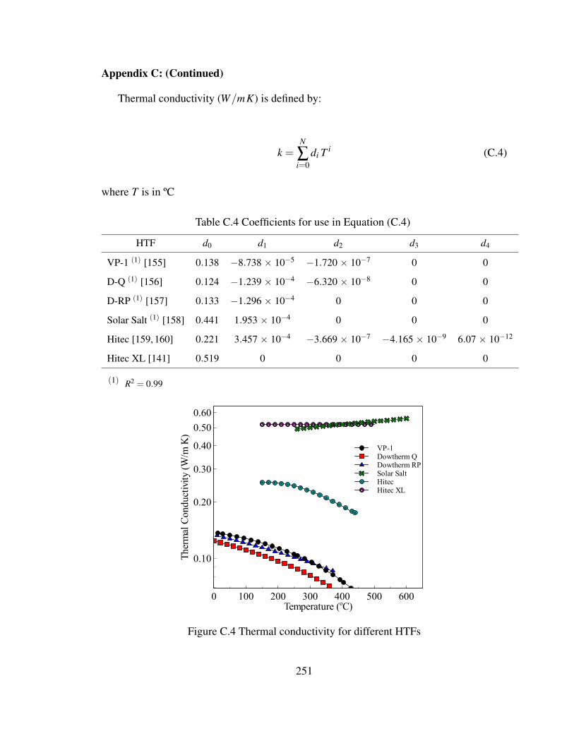
Appendix C: (Continued)

Thermal conductivity (W/mK) is defined by:

k =N

∑i=0

di T i (C.4)

where T is in ºC

Table C.4 Coefficients for use in Equation (C.4)

HTF d0 d1 d2 d3 d4

VP-1 (1) [155] 0.138 −8.738 × 10−5 −1.720 × 10−7 0 0

D-Q (1) [156] 0.124 −1.239 × 10−4 −6.320 × 10−8 0 0

D-RP (1) [157] 0.133 −1.296 × 10−4 0 0 0

Solar Salt (1) [158] 0.441 1.953 × 10−4 0 0 0

Hitec [159, 160] 0.221 3.457 × 10−4 −3.669 × 10−7 −4.165 × 10−9 6.07 × 10−12

Hitec XL [141] 0.519 0 0 0 0

(1) R2 = 0.99

VP-1Dowtherm QDowtherm RPSolar SaltHitecHitec XL

Ther

mal

Con

duct

ivity

(W/m

K)

0.10

0.20

0.30

0.40

0.500.60

Temperature (oC)0 100 200 300 400 500 600

Figure C.4 Thermal conductivity for different HTFs

251

Appendix C: (Continued)

Absolute viscosity (cP) is defined by:

ln µ =N

∑i=0

ei T i (C.5)

For Hitec and Hitec XL the next equation is used:

ln µ =N

∑i=0

ei (ln T )i (C.6)

For solar salt:

µ =N

∑i=0

ei T i (C.7)

where T is in ºC

Table C.5 Coefficients for use in Equations (C.5)-(C.7)

HTF e0 e1 e2 e3 e4

VP-1 (1) [155] 2.008 −2.989 × 10−2 1.207 × 10−4 −2.714 × 10−7 2.370 × 10−10

D-Q (1) [156] 2.125 −3.960 × 10−2 2.090 × 10−4 −5.935 × 10−7 6.460 × 10−10

D-RP (1) [157] 5.147 −7.174 × 10−2 3.981 × 10−4 −1.087 × 10−6 1.108 × 10−9

Solar Salt (1) [158] 22.713 −1.200 × 10−1 2.281 × 10−4 −1.474 × 10−7 0

Hitec (1) [159, 160] 33.324 −9.270 6.364 × 10−1 0 0

Hitec XL (2) [141] 14.132 −3.364 0 0 0

(1) R2 = 0.99(2) R2 is not given

252

Appendix C: (Continued)

VP-1Dowtherm QDowtherm RPSolar SaltHitecHitec XL

Visc

osity

(cP)

0.1

1

10

100

Temperature (oC)0 100 200 300 400 500 600

Figure C.5 Absolute viscosity for different HTFs

253

Appendix C: (Continued)

Vapor pressure (kPa) is defined by:

Pv =N

∑i=0

fi T i (C.8)

where T is in ºC

Table C.6 Coefficients for use in Equation (C.8)

HTF f0 f1 f2 f3 f4

VP-1 (1) [155] 0.789 −1.379 × 10−1 3.783 × 10−3 −3.387 × 10−5 1.056 × 10−7

D-Q (1) [156] 24.738 −7.325 × 10−1 8.525 × 10−3 −4.684 × 10−5 1.080 × 10−7

D-RP (2) [157] −354.560 4.768 −2.155 × 10−2 3.318 × 10−5 0

(1) R2 = 0.99(2) R2 = 1.00

VP-1Dowtherm QDowtherm RP

Vapo

r Pre

ssur

e (M

Pa)

0

0.2

0.4

0.6

0.8

1

1.2

1.4

1.6

Temperature (oC)50 100 150 200 250 300 350 400 450

Figure C.6 Vapor pressure for different HTFs

254

Appendix D: Pipe Geometry

Table D.1 Wall thickness, in mm, for different nominal pipe sizes (Pipe Schedule A-G).Adapted from [141]

Nominal Pipe Schedule

Pipe Size, in A B C D E F G

2.5 2.11 3.05 5.16 7.01 9.53 14.02 . . .

3 2.11 3.05 5.49 7.62 11.13 15.24 . . .

4 2.11 3.05 3.96 4.78 6.02 8.56 11.136 2.77 3.40 4.78 7.11 10.97 14.27 18.268 2.77 3.76 6.35 7.04 8.18 10.31 12.7010 3.40 4.19 4.78 6.35 7.80 9.27 12.7012 3.96 4.57 6.35 8.38 9.53 10.31 12.7014 4.78 6.35 7.92 9.53 11.13 12.70 15.0916 4.78 6.35 7.92 9.53 12.70 14.35 21.4418 4.78 6.35 7.92 9.53 11.13 12.70 14.2720 5.54 6.35 9.53 12.70 15.09 20.62 26.1922 6.35 9.53 12.70 22.23 28.58 34.93 41.2824 6.35 9.53 12.70 14.27 17.48 24.61 30.9626 7.92 9.53 12.70 . . . . . . . . . . . .

28 7.92 9.53 12.70 15.88 . . . . . . . . .

30 7.92 9.53 12.70 15.88 . . . . . . . . .

32 7.92 9.53 12.70 15.88 17.48 . . . . . .

34 7.92 9.53 12.70 15.88 17.48 . . . . . .

36 7.92 9.53 12.70 15.88 19.05 . . . . . .

42 9.53 12.70 15.88 19.05 . . . . . . . . .

48 9.53 12.70 19.05 25.40 . . . . . . . . .

54 9.53 12.70 19.05 25.40 . . . . . . . . .

60 9.53 12.70 19.05 25.40 . . . . . . . . .

66 9.53 12.70 19.05 25.40 . . . . . . . . .

72 9.53 12.70 19.05 25.40 . . . . . . . . .

255

Appendix D: (Continued)

Table D.2 Wall thickness, in mm, for different nominal pipe sizes (Pipe Schedule H-M).Adapted from [141]

Nominal Pipe Schedule

Pipe Size, in H I J K L M

2.5 . . . . . . . . . . . . . . . . . .

3 . . . . . . . . . . . . . . . . . .

4 13.49 17.12 . . . . . . . . . . . .

6 21.95 . . . . . . . . . . . . . . .

8 15.09 18.26 20.62 22.23 23.01 . . .

10 15.09 18.26 21.44 25.40 28.58 . . .

12 14.27 17.48 21.44 25.40 28.58 33.3214 19.05 23.83 27.79 31.75 35.71 . . .

16 26.19 30.96 36.53 40.49 . . . . . .

18 19.05 23.83 29.36 34.93 39.67 45.2420 32.54 38.10 44.45 50.01 . . . . . .

22 47.63 53.98 . . . . . . . . . . . .

24 38.89 46.02 52.37 59.54 . . . . . .

26 . . . . . . . . . . . . . . . . . .

28 . . . . . . . . . . . . . . . . . .

30 . . . . . . . . . . . . . . . . . .

32 . . . . . . . . . . . . . . . . . .

34 . . . . . . . . . . . . . . . . . .

36 . . . . . . . . . . . . . . . . . .

42 . . . . . . . . . . . . . . . . . .

48 . . . . . . . . . . . . . . . . . .

54 . . . . . . . . . . . . . . . . . .

60 . . . . . . . . . . . . . . . . . .

66 . . . . . . . . . . . . . . . . . .

72 . . . . . . . . . . . . . . . . . .

256

Appendix D: (Continued)

Table D.3 Inside diameter, in mm, for different nominal pipe sizes (Pipe Schedule A-G).Adapted from [141]

Nominal Pipe Schedule

Pipe Size, in A B C D E F G

2.5 68.8 66.9 62.7 59.0 54.0 45.0 . . .

3 84.7 82.8 77.9 73.7 66.6 58.4 . . .

4 110.1 108.2 106.4 104.7 102.3 97.2 92.06 162.7 161.5 158.7 154.1 146.3 139.7 131.78 213.5 211.6 206.4 205.0 202.7 198.5 193.7

10 266.2 264.7 263.5 260.4 257.5 254.5 247.712 315.9 314.7 311.2 307.1 304.8 303.2 298.514 346.0 342.9 339.8 336.6 333.3 330.2 325.416 396.8 393.7 390.6 387.4 381.0 377.7 363.518 447.6 444.5 441.4 438.2 434.9 431.8 428.720 496.9 495.3 489.0 482.6 477.8 466.8 455.622 546.1 539.8 533.4 514.4 501.7 489.0 476.324 596.9 590.6 584.2 581.1 574.6 560.4 547.726 644.6 641.4 635.0 . . . . . . . . . . . .

28 695.4 692.2 685.8 679.5 . . . . . . . . .

30 746.2 743.0 736.6 730.3 . . . . . . . . .

32 797.0 793.8 787.4 781.1 777.8 . . . . . .

34 847.8 844.6 838.2 831.9 828.6 . . . . . .

36 898.6 895.4 889.0 882.7 876.3 . . . . . .

42 1047.8 1041.4 1035.1 1028.7 . . . . . . . . .

48 1200.2 1193.8 1181.1 1168.4 . . . . . . . . .

54 1352.6 1346.2 1333.5 1320.8 . . . . . . . . .

60 1505.0 1498.6 1485.9 1473.2 . . . . . . . . .

66 1657.4 1651.0 1638.3 1625.6 . . . . . . . . .

72 1809.8 1803.4 1790.7 1778.0 . . . . . . . . .

257

Appendix D: (Continued)

Table D.4 Inside diameter, in mm, for different nominal pipe sizes (Pipe Schedule H-M).Adapted from [141]

Nominal Pipe Schedule

Pipe Size, in H I J K L M

2.5 . . . . . . . . . . . . . . . . . .

3 . . . . . . . . . . . . . . . . . .

4 87.3 80.1 . . . . . . . . . . . .

6 124.4 . . . . . . . . . . . . . . .

8 188.9 182.5 177.8 174.6 173.1 . . .

10 242.9 236.5 230.2 222.3 215.9 . . .

12 295.3 288.9 281.0 273.1 266.7 257.214 317.5 307.9 300.0 292.1 284.2 . . .

16 354.0 344.5 333.3 325.4 . . . . . .

18 419.1 409.5 398.5 387.4 377.9 366.720 442.9 431.8 419.1 408.0 . . . . . .

22 463.6 450.9 . . . . . . . . . . . .

24 531.8 517.6 504.9 490.5 . . . . . .

26 . . . . . . . . . . . . . . . . . .

28 . . . . . . . . . . . . . . . . . .

30 . . . . . . . . . . . . . . . . . .

32 . . . . . . . . . . . . . . . . . .

34 . . . . . . . . . . . . . . . . . .

36 . . . . . . . . . . . . . . . . . .

42 . . . . . . . . . . . . . . . . . .

48 . . . . . . . . . . . . . . . . . .

54 . . . . . . . . . . . . . . . . . .

60 . . . . . . . . . . . . . . . . . .

66 . . . . . . . . . . . . . . . . . .

72 . . . . . . . . . . . . . . . . . .

258

About the Author

Ricardo Vasquez Padilla was born in Barranquilla, Colombia in March 1978. He pur-

sued his bachelor and master at Universidad del Norte in Mechanical Engineering. After

he got married with his beloved Jennifer, he began doctoral studies at University of South

Florida under the guidance of Dr. Yogi Goswami and Dr. Elias Stefanakos in the Clean

Energy Research Center (CERC). Initially, he worked in the experimental and theoreti-

cal analysis of the Goswami cycle and then on the design of parabolic trough (PTC) solar

power plants. In August 2010 his first son Noah was born. Upon graduation, the author will

return to Universidad del Norte, there he will work as faculty member in the Department

of Mechanical Engineering in the area of renewable energy.

259