analysis of the heterogeneous multiscale method for parabolic ...

MATHEMATICS OF COMPUTATIONVolume 76, Number 257, January 2007, Pages 153–177S 0025-5718(06)01909-0Article electronically published on October 10, 2006

ANALYSIS OF THE HETEROGENEOUS MULTISCALE METHODFOR PARABOLIC HOMOGENIZATION PROBLEMS

PINGBING MING AND PINGWEN ZHANG

Abstract. The heterogeneous multiscale method (HMM) is applied to var-ious parabolic problems with multiscale coefficients. These problems can beeither linear or nonlinear. Optimal estimates are proved for the error betweenthe HMM solution and the homogenized solution.

1. Introduction and main results

1.1. Generality. Consider the following parabolic problem:

(1.1)

⎧⎪⎨⎪⎩∂tu

ε −∇ · (aε∇uε) = f in D × (0, T ) =: Q,

uε = 0 on ∂D × (0, T ),

uε|t=0 = u0.

Here ε is a small parameter that signifies the multiscale nature of the problem. Welet D be a bounded domain in R

d and T a positive real number. A problem of thistype is interesting because of its simplicity and its relevance to several importantpractical problems, such as the flow in porous media and the mechanical propertiesof composite materials. In contrast to the elliptic problems there may be oscillationsin the temporal direction besides the oscillation in the spatial direction.

On the analytic side, the following fact is known about (1.1). In the sense ofparabolic H-convergence (see [25], [8], [12]), introduced with minor modificationby Spagnolo and Colombini under the name of G-convergence or PG-convergence(see [11], [22], [23], [24]), for every f ∈ L2(0, T ; H−1(D)) and u0 ∈ L2(D), thesequence uε the solutions of (1.1) satisfies

uε U weakly in L2(0, T ; H10 (D)),

aε∇uε A∇U weakly in L2(Q; Rd),

Received by the editor June 3, 2003 and, in revised form, December 6, 2005.2000 Mathematics Subject Classification. Primary 65N30, 35K05, 65N15.Key words and phrases. Heterogeneous multiscale method, parabolic homogenization prob-

lems, finite element methods.The first author was partially supported by the National Natural Science Foundation of China

under the grant 10571172 and also supported by the National Basic Research Program under thegrant 2005CB321704.

The second author was partially supported by National Natural Science Foundation of Chinafor Distinguished Young Scholars 10225103 and also supported by the National Basic ResearchProgram under the grant 2005CB321704.

c©2006 American Mathematical SocietyReverts to public domain 28 years from publication

153

154 P.-B. MING AND P.-W. ZHANG

where U is the unique solution of the problem

(1.2)

⎧⎪⎨⎪⎩∂tU −∇ · (A∇U) = f in Q,

U = 0 on ∂D × (0, T ],

U |t=0 = u0.

In general, there are no explicit formulas for the effective matrix A.Classical numerical methods for this problem are designed to resolve the full

details of the fine scale problem (1.1) and without taking into account the specialfeatures of the coefficient matrix aε. In contrast, the modern multiscale methodsare designed specifically for retrieving partial information about uε with sublinearcost [16], i.e., the total cost grows sublinearly with the cost of solving the full finescale problem. To this end, the methods have to take full advantage of the specialfeatures of the problem such as scale separation and self-similarity of the solution.One cannot hope to get an algorithm with sublinear cost for a fully general problem.

The heterogeneous multiscale method introduced in [15] is a general method-ology for designing a sublinear algorithm by exploiting the scale separation andother special features of the problem. HMM consists of two ingredients: an overallmacroscopic scheme for macrovariables on a macrogrid and estimating the miss-ing macroscopic data from the microscopic model. The efficiency of HMM lies inthe ability to extract the missing macroscale data from microscale models withminimum cost, by exploiting scale separation.

For (1.1), the macroscopic solver is chosen to be the standard piecewise linearfinite element method [10] over a macroscopic triangulation TH with mesh size H asthe spatial solver, and the backward Euler scheme as the temporal discretization.Many other conventional discretization methods could be proper candidates as themacroscopic solver. For example, the finite difference method and the discontinuousGalerkin method have been employed as the macroscopic solver in [1] and [9],respectively.

We formulate our method as follows. For 1 ≤ k ≤ n, let tk = k∆t with ∆t = T/n.Let U0

H = QHu0 with QH the L2 projection operator from H10 (D) to XH , where

XH is the macroscopic finite element space. Let UkH ∈ XH be the solution of the

problem

(1.3) (∂UkH , V ) + AH(tk; Uk

H , V ) = (fk, V ) for all V ∈ XH ,

where ∂UkH = (Uk

H − Uk−1H )/∆t and fk = ∆t−1

∫ tk+∆t

tkf(x, s) ds.

It remains to estimate the stiffness matrix, which amounts to evaluating theeffective bilinear form AH(tn; V, W ) for any V, W ∈ XH . We write AH as

AH(tn; V, W ) =∫D

∇W · AH(x, tn)∇V dx =∑

K∈TH

∫K

∇W · AH(x, tn)∇V dx

∑

K∈TH

|K|∇W · AH(xK , tn)∇V,

where xK is the barycenter of K. We approximate AH(xK , tn) by solving theCauchy-Dirichlet problem:

(1.4)

⎧⎪⎨⎪⎩∂tv

ε −∇ ·(aε∇vε

)= 0 in (xK + Iδ) × (tn, tn + τn),

vε = V on ∂Iδ × (tn, tn + τn),

vε|t=tn= V.

HMM FOR PARABOLIC PROBLEM 155

We then let

∇W · AH(xK , tn)∇V 1τn|Iδ|

tn+τn∫tn

∫Iδ

∇wε · aε∇vε dx dt,

where τn denotes the microsimulation time that evolves in nth macrotime step,and Iδ = δY with the unit cell Y : = (−1/2, 1/2)d. For simplicity, we denoteIδ := xK + Iδ, Tn: = (tn, tn + τn), and the cylinder Qn: = Iδ × Tn. We thus rewriteAH as

(1.5) AH(tn; V, W ): =∑

K∈TH

|K||Qn|

∫Qn

∇wε · aε∇vε dx dt.

In (1.4), we use the Dirichlet boundary condition and the Cauchy initial con-dition. One may also use other boundary conditions and initial conditions. Forexample, we may use the Neumann or periodic boundary condition and the peri-odic initial condition. In the case when aε = a(x, x/ε, t) and a(x, y, t) is periodicin y, one can take Iδ to be xK + εY and impose the boundary/initial conditions,as vε − V is periodic on the boundary of the cylinder (xK + εY ) × (tn, tn + ε2).

So far, the algorithm is quite general. The saving compared with solving the fullfine scale problem comes from the fact that we may choose Iδ and τk much smallerthan K and ∆t, respectively. The size of the microcell Iδ and the microsimulationtime τk are mainly determined by the accuracy, the cost, and the microstructureof aε. The main purpose of the error analysis presented below is to help to assessthe performance of the method and give guidance for the designing of the methods,namely, how we choose δ and τk, or types of cell problems.

Since HMM is based on standard macroscale numerical methods and uses themicroscale model only as a supplement, it is possible to analyze its stability andaccuracy properties using the traditional framework of numerical analysis. Thishas already been illustrated in [14, 15, 17] and will be further elaborated in thepresent paper. Roughly speaking, we will show that HMM is stable whenever themacroscopic solver is stable. The overall error between the HMM solution and thehomogenized solution is controlled by the accuracy of the macroscopic solver, andthe consistency error emanates from the estimate of the macroscopic data from themicroscopic model, which will be denoted by e(HMM). Next we estimate e(HMM)for two cases. One is aε = a(x, x/ε, t) with a(x, y, t) periodic in y, and the other isaε = a(x, x/ε, t, t/ε2) with a(x, y, t, s) periodic in y and s.

We will always assume that aε(x, t) is symmetric and uniformly elliptic:

λI ≤ aε ≤ ΛI

for some λ, Λ > 0. We will use |·| to denote the abstract value of a scalar quantityand the volume of a set.

Throughout this paper, the generic constant C is assumed to be independentof the microscale ε, the mesh size H, the time step ∆t, the cell size δ, and themicrosimulation time τkn

k=1. We use the summation convention.

1.2. Main results. Define

(1.6) e(HMM) = max1≤k≤n

ek(HMM)


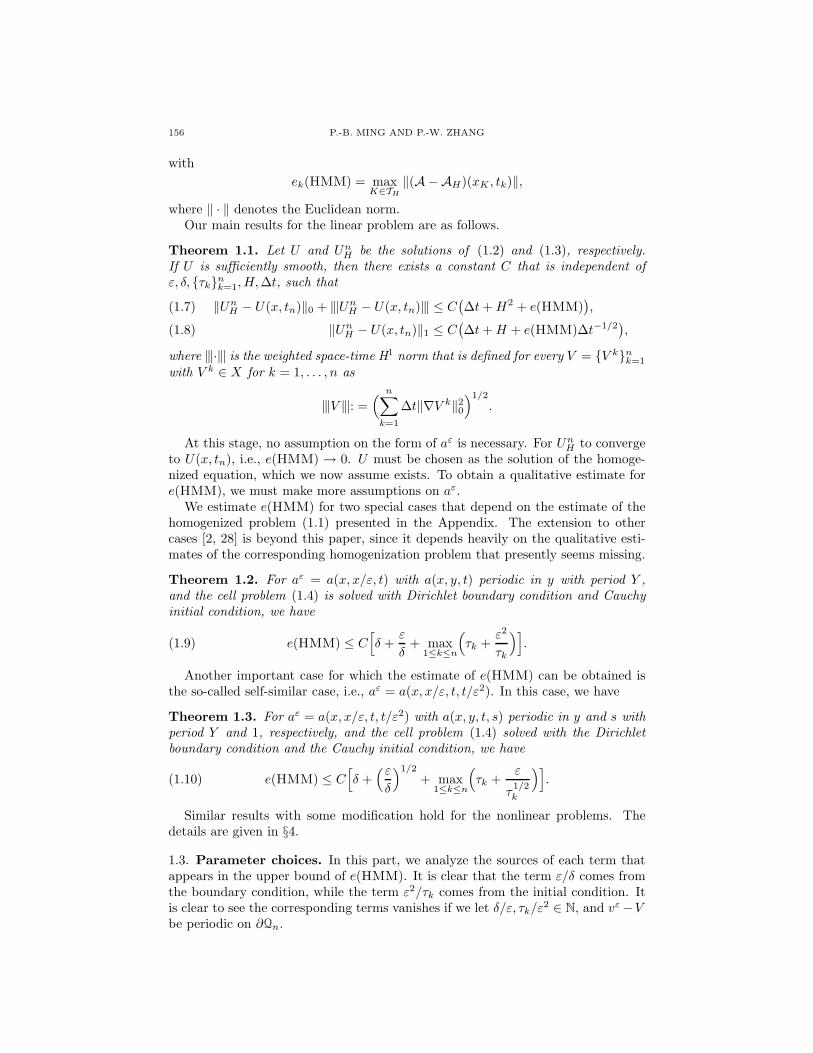
withek(HMM) = max

K∈TH

‖(A−AH)(xK , tk)‖,

where ‖ · ‖ denotes the Euclidean norm.Our main results for the linear problem are as follows.

Theorem 1.1. Let U and UnH be the solutions of (1.2) and (1.3), respectively.

If U is sufficiently smooth, then there exists a constant C that is independent ofε, δ, τkn

k=1, H, ∆t, such that

‖UnH − U(x, tn)‖0 + |||Un

H − U(x, tn)||| ≤ C(∆t + H2 + e(HMM)

),(1.7)

‖UnH − U(x, tn)‖1 ≤ C

(∆t + H + e(HMM)∆t−1/2

),(1.8)

where |||·||| is the weighted space-time H1 norm that is defined for every V = V knk=1

with V k ∈ X for k = 1, . . . , n as

|||V |||: =( n∑

k=1

∆t‖∇V k‖20

)1/2

.

At this stage, no assumption on the form of aε is necessary. For UnH to converge

to U(x, tn), i.e., e(HMM) → 0. U must be chosen as the solution of the homoge-nized equation, which we now assume exists. To obtain a qualitative estimate fore(HMM), we must make more assumptions on aε.

We estimate e(HMM) for two special cases that depend on the estimate of thehomogenized problem (1.1) presented in the Appendix. The extension to othercases [2, 28] is beyond this paper, since it depends heavily on the qualitative esti-mates of the corresponding homogenization problem that presently seems missing.

Theorem 1.2. For aε = a(x, x/ε, t) with a(x, y, t) periodic in y with period Y ,and the cell problem (1.4) is solved with Dirichlet boundary condition and Cauchyinitial condition, we have

(1.9) e(HMM) ≤ C[δ +

ε

δ+ max

1≤k≤n

(τk +

ε2

τk

)].

Another important case for which the estimate of e(HMM) can be obtained isthe so-called self-similar case, i.e., aε = a(x, x/ε, t, t/ε2). In this case, we have

Theorem 1.3. For aε = a(x, x/ε, t, t/ε2) with a(x, y, t, s) periodic in y and s withperiod Y and 1, respectively, and the cell problem (1.4) solved with the Dirichletboundary condition and the Cauchy initial condition, we have

(1.10) e(HMM) ≤ C[δ +

(ε

δ

)1/2

+ max1≤k≤n

(τk +

ε

τ1/2k

)].

Similar results with some modification hold for the nonlinear problems. Thedetails are given in §4.

1.3. Parameter choices. In this part, we analyze the sources of each term thatappears in the upper bound of e(HMM). It is clear that the term ε/δ comes fromthe boundary condition, while the term ε2/τk comes from the initial condition. Itis clear to see the corresponding terms vanishes if we let δ/ε, τk/ε2 ∈ N, and vε −Vbe periodic on ∂Qn.


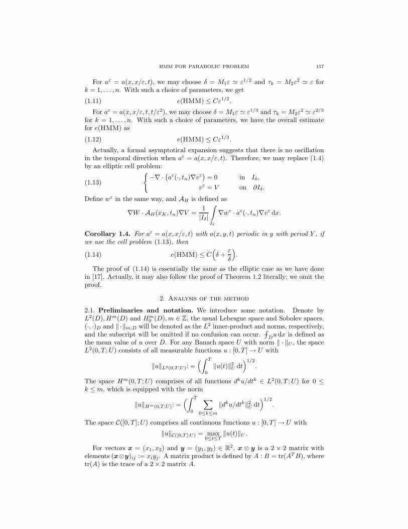
For aε = a(x, x/ε, t), we may choose δ = M1ε ε1/2 and τk = M2ε2 ε for

k = 1, . . . , n. With such a choice of parameters, we get

(1.11) e(HMM) ≤ Cε1/2.

For aε = a(x, x/ε, t, t/ε2), we may choose δ = M1ε ε1/3 and τk = M2ε2 ε2/3

for k = 1, . . . , n. With such a choice of parameters, we have the overall estimatefor e(HMM) as

(1.12) e(HMM) ≤ Cε1/3.

Actually, a formal asymptotical expansion suggests that there is no oscillationin the temporal direction when aε = a(x, x/ε, t). Therefore, we may replace (1.4)by an elliptic cell problem:

(1.13)

−∇ ·

(aε(·, tn)∇vε

)= 0 in Iδ,

vε = V on ∂Iδ.

Define wε in the same way, and AH is defined as

∇W · AH(xK , tn)∇V =1|Iδ|

∫Iδ

∇wε · aε(·, tn)∇vε dx.

Corollary 1.4. For aε = a(x, x/ε, t) with a(x, y, t) periodic in y with period Y , ifwe use the cell problem (1.13), then

(1.14) e(HMM) ≤ C(δ +

ε

δ

).

The proof of (1.14) is essentially the same as the elliptic case as we have donein [17]. Actually, it may also follow the proof of Theorem 1.2 literally; we omit theproof.

2. Analysis of the method

2.1. Preliminaries and notation. We introduce some notation. Denote byL2(D), Hm(D) and Hm

0 (D), m ∈ Z, the usual Lebesgue space and Sobolev spaces.(·, ·)D and ‖ ·‖m,D will be denoted as the L2 inner-product and norms, respectively,and the subscript will be omitted if no confusion can occur.

∫−

Du dx is defined as

the mean value of u over D. For any Banach space U with norm ‖ · ‖U , the spaceL2(0, T ; U) consists of all measurable functions u : [0, T ] → U with

‖u‖L2(0,T ;U): =(∫ T

0

‖u(t)‖2U dt

)1/2

.

The space Hm(0, T ; U) comprises of all functions dku/dtk ∈ L2(0, T ; U) for 0 ≤k ≤ m, which is equipped with the norm

‖u‖Hm(0,T ;U): =(∫ T

0

∑0≤k≤m

‖dku/dtk‖2U dt

)1/2

.

The space C([0, T ]; U) comprises all continuous functions u : [0, T ] → U with

‖u‖C([0,T ];U) = max0≤t≤T

‖u(t)‖U .

For vectors x = (x1, x2) and y = (y1, y2) ∈ R2, x ⊗ y is a 2 × 2 matrix with

elements (x⊗y)ij := xiyj . A matrix product is defined by A : B = tr(AT B), wheretr(A) is the trace of a 2 × 2 matrix A.


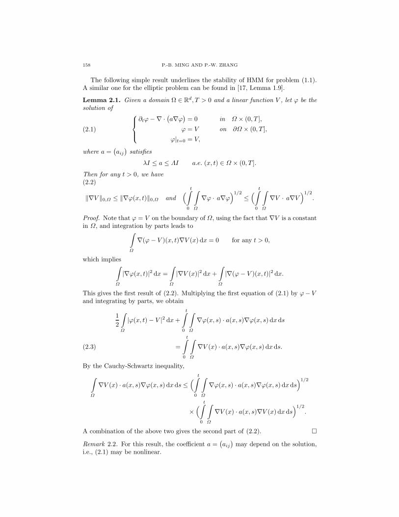
The following simple result underlines the stability of HMM for problem (1.1).A similar one for the elliptic problem can be found in [17, Lemma 1.9].

Lemma 2.1. Given a domain Ω ∈ Rd, T > 0 and a linear function V , let ϕ be the

solution of

(2.1)

⎧⎪⎨⎪⎩∂tϕ −∇ ·

(a∇ϕ

)= 0 in Ω × (0, T ],

ϕ = V on ∂Ω × (0, T ],

ϕ|t=0 = V,

where a =(aij

)satisfies

λI ≤ a ≤ ΛI a.e. (x, t) ∈ Ω × (0, T ].

Then for any t > 0, we have(2.2)

‖∇V ‖0,Ω ≤ ‖∇ϕ(x, t)‖0,Ω and( t∫

0

∫Ω

∇ϕ · a∇ϕ)1/2

≤( t∫

0

∫Ω

∇V · a∇V)1/2

.

Proof. Note that ϕ = V on the boundary of Ω, using the fact that ∇V is a constantin Ω, and integration by parts leads to∫

Ω

∇(ϕ − V )(x, t)∇V (x) dx = 0 for any t > 0,

which implies∫Ω

|∇ϕ(x, t)|2 dx =∫Ω

|∇V (x)|2 dx +∫Ω

|∇(ϕ − V )(x, t)|2 dx.

This gives the first result of (2.2). Multiplying the first equation of (2.1) by ϕ− Vand integrating by parts, we obtain

12

∫Ω

|ϕ(x, t) − V |2 dx +

t∫0

∫Ω

∇ϕ(x, s) · a(x, s)∇ϕ(x, s) dx ds

=

t∫0

∫Ω

∇V (x) · a(x, s)∇ϕ(x, s) dx ds.(2.3)

By the Cauchy-Schwartz inequality,∫Ω

∇V (x) · a(x, s)∇ϕ(x, s) dx ds ≤( t∫

0

∫Ω

∇ϕ(x, s) · a(x, s)∇ϕ(x, s) dx ds)1/2

×( t∫

0

∫Ω

∇V (x) · a(x, s)∇V (x) dx ds)1/2

.

A combination of the above two gives the second part of (2.2).

Remark 2.2. For this result, the coefficient a =(aij

)may depend on the solution,

i.e., (2.1) may be nonlinear.


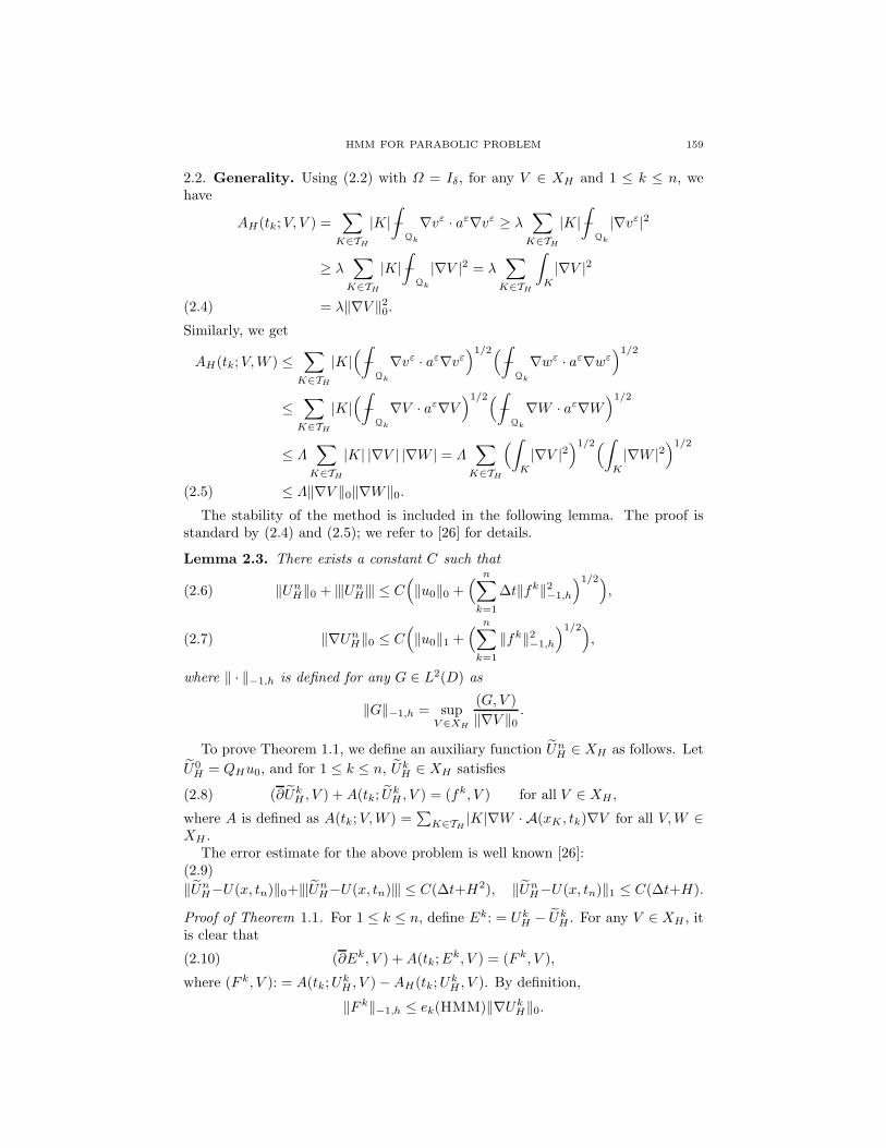
2.2. Generality. Using (2.2) with Ω = Iδ, for any V ∈ XH and 1 ≤ k ≤ n, wehave

AH(tk; V, V ) =∑

K∈TH

|K|∫−

Qk

∇vε · aε∇vε ≥ λ∑

K∈TH

|K|∫−

Qk

|∇vε|2

≥ λ∑

K∈TH

|K|∫−

Qk

|∇V |2 = λ∑

K∈TH

∫K

|∇V |2

= λ‖∇V ‖20.(2.4)

Similarly, we get

AH(tk; V, W ) ≤∑

K∈TH

|K|(∫−

Qk

∇vε · aε∇vε)1/2(∫

−Qk

∇wε · aε∇wε)1/2

≤∑

K∈TH

|K|(∫−

Qk

∇V · aε∇V)1/2(∫

−Qk

∇W · aε∇W)1/2

≤ Λ∑

K∈TH

|K| |∇V | |∇W | = Λ∑

K∈TH

(∫K

|∇V |2)1/2(∫

K

|∇W |2)1/2

≤ Λ‖∇V ‖0‖∇W‖0.(2.5)

The stability of the method is included in the following lemma. The proof isstandard by (2.4) and (2.5); we refer to [26] for details.

Lemma 2.3. There exists a constant C such that

‖UnH‖0 + |||Un

H ||| ≤ C(‖u0‖0 +

( n∑k=1

∆t‖fk‖2−1,h

)1/2),(2.6)

‖∇UnH‖0 ≤ C

(‖u0‖1 +

( n∑k=1

‖fk‖2−1,h

)1/2),(2.7)

where ‖ · ‖−1,h is defined for any G ∈ L2(D) as

‖G‖−1,h = supV ∈XH

(G, V )‖∇V ‖0

.

To prove Theorem 1.1, we define an auxiliary function UnH ∈ XH as follows. Let

U0H = QHu0, and for 1 ≤ k ≤ n, Uk

H ∈ XH satisfies

(2.8) (∂UkH , V ) + A(tk; Uk


where A is defined as A(tk; V, W ) =∑

K∈TH|K|∇W · A(xK , tk)∇V for all V, W ∈

XH .The error estimate for the above problem is well known [26]:

(2.9)‖Un

H−U(x, tn)‖0+|||UnH−U(x, tn)||| ≤ C(∆t+H2), ‖Un

H−U(x, tn)‖1 ≤ C(∆t+H).

Proof of Theorem 1.1. For 1 ≤ k ≤ n, define Ek: = UkH − Uk

H . For any V ∈ XH , itis clear that

(2.10) (∂Ek, V ) + A(tk; Ek, V ) = (F k, V ),

where (F k, V ): = A(tk; UkH , V ) − AH(tk; Uk

H , V ). By definition,

‖F k‖−1,h ≤ ek(HMM)‖∇UkH‖0.


By (2.6) we have, since E0 = 0,

(2.11) ‖En‖0 + |||En||| ≤ Ce(HMM)|||UnH ||| ≤ Ce(HMM).

Combining the above inequality and the first part of (2.9), we obtain (1.7).Repeating the above steps, using (2.7) and (2.6), we obtain

‖∇En‖0 ≤ Ce(HMM)∆t−1/2|||UnH ||| ≤ Ce(HMM)∆t−1/2.

The estimate (1.8) follows from the above estimate and the second part of (2.9).

Remark 2.4. Noting that En ∈ XH for any n, and using (2.11) and the inverseestimate [10], we get

‖En‖1 ≤ (C/H)‖En‖0 ≤ Ce(HMM)/H,

which together with the second part of (2.9) leads to

(2.12) ‖UnH − U(x, tn)‖1 ≤ C(H + ∆t + e(HMM)/H).

3. Estimating e(HMM)

In this section, we estimate e(HMM) for two cases: one is aε = a(x, x/ε, t) andthe other is aε = a(x, x/ε, t, t/ε2). In both cases, the cell problem (1.4) is solvedwith the Dirichlet boundary condition and the Cauchy initial condition. We willuse aε

K,n = a(xK , x/ε, tn) or aεK,n = a(xK , x/ε, tn, t/ε2) and χK,n = χ(xK , x/ε, tn)

or χK,n = χ(xK , x/ε, tn, t/ε2) for simplicity, where χ is the solution of certain cellproblems (cf. (3.4) and (3.15)).

Estimating e(HMM) consists of two steps. First, we estimate ‖A − A‖. Theauxiliary operator A is defined by

(3.1) ∇W · A(xK , tn)∇V =∫−

Qn

∇W ε · aεK,n∇V ε for any W, V ∈ XH ,

whereV ε = V + εχK,n · ∇V and W ε = W + εχK,n · ∇W.

Next we estimate ‖A − AH‖. This is achieved by

∇W · (A − AH)(xK , tn)∇V

=∫−

Qn

[∇W ε · aεK,n∇(V ε − vε) + ∇V ε · aε

K,n∇(W ε − wε)](3.2)

−∫−

Qn

[∇wε · (aε − aεK,n)∇vε + ∇(wε − W ε) · aε

K,n∇(vε − V ε)].

Finally, estimating e(HMM) follows from the triangle inequality.

3.1. Estimating e(HMM) for the case when aε = a(x, x/ε, t). Denote by vε

the solution of (1.4) with aε replaced by aεK,n. By a standard a priori estimate

and (2.2), we have

(3.3) ‖∇(vε − vε)‖L2(Qn) ≤ C(δ + τn)‖∇vε‖L2(Qn) ≤ C(δ + τn)‖∇V ‖L2(Qn).

For j = 1, . . . , d, χ = χjdj=1 is periodic in y with period Y and satisfies

(3.4)∂

∂yi

(aik

∂χj

∂yk

)(x, y, t) = −

( ∂

∂yiaij

)(x, y, t) in Y,

∫Y

χj(x, y, t) dy = 0.


This problem is solvable, and there exists a constant C such that for j = 1, . . . , d,

(3.5) |∇yχj(x, y, t)| ≤ C for all (x, t) ∈ Q and y ∈ Y.

The effective matrix is given by

(3.6) Aij(x, t) =∫−

Y

(aij + aik

∂χj

∂yk

)(x, y, t) dy i, j = 1, . . . , d.

A straightforward calculation gives

(3.7) ∇ ·(aε

K,n∇V ε)

= 0 and ∇ ·(aε

K,n∇W ε)

= 0.

Define θε = vε − V ε, which obviously satisfies

(3.8)

⎧⎪⎨⎪⎩∂tθ

ε −∇ ·(aε

K,n∇θε)

= 0 in Qn,

θε = −εχK,n · ∇V on ∂Iδ × Tn,

θε|t=tn= −εχK,n · ∇V.

Lemma 3.1. Let θε be solution of (3.8). There exists a constant independent ofε, δ, and τn such that

(3.9) ‖∇θε‖L2(Qn) ≤ C( ε

τ1/2n

+(ε

δ

)1/2)‖∇V ‖L2(Qn).

Proof. Multiplying both sides of (3.8)1 by θε1: = θε+(V ε−V )(1−ρε) and integrating

over Iδ, we obtain

(3.10)12

∂

∂t

∫Iδ

|θε1|2 +

∫Iδ

∇θε1 · aε

K,n∇θε1 =

∫Iδ

∇(θε1 − θε) · aε

K,n∇θε1,

where the cut-off function ρε ∈ C∞0 (Iδ), |∇ρε| ≤ C/ε, and

ρε =

1 if dist(x, ∂Iδ) ≥ 2ε,

0 if dist(x, ∂Iδ) ≤ ε.

It is clear to see that

|∫

Iδ

∇(θε1−θε)·aε

K,n∇θε1|≤

(∫Iδ

∇(θε1−θε)·aε

K,n∇(θε1−θε)

)1/2

(∫Iδ

∇θε1·aε

K,n∇θε1

)1/2

.

Substituting the above inequality into (3.10), we obtain∂

∂t

∫Iδ

|θε1|2 +

∫Iδ

∇θε1 · aε

K,n∇θε1 ≤

∫Iδ

∇(θε1 − θε) · aε

K,n∇(θε1 − θε).

Integrating the above inequality over Tn, we get

λ‖∇θε1‖2

L2(Qn) ≤ ‖θε1(x, tn)‖2

L2(Iδ) + Λ‖∇(θε1 − θε)‖2

L2(Qn),

which implies

‖∇θε‖L2(Qn) ≤ λ−1/2‖θε1(x, tn)‖L2(Iδ) +

(1 + (Λ/λ)1/2

)‖∇(θε

1 − θε)‖L2(Qn).

A direct calculation gives

‖∇(θε1 − θε)‖L2(Qn) ≤ C

(ε

δ

)1/2

‖∇V ‖L2(Qn),

‖θε1(x, tn)‖L2(Iδ) = ε‖ρε(V ε − V )‖L2(Iδ) ≤ Cε‖∇V ‖L2(Iδ).

A combination of the above three inequalities leads to (3.9).

Next lemma concerns estimating ‖A − A‖.



(3.11) ‖(A − A)(xK , tn)‖ ≤ Cε

δ.

Proof. Denote by Iκε = κY , where κ is the integer part of δ/ε, i.e., κ = δ/ε,integrating by parts and using (3.7), we get∫

−Iκε

∇(W ε − W ) · aεK,n∇V ε = 0.

Using the expression of V ε and (3.6), we obtain∫−

Iκε

∇W · aεK,n∇V ε = ∇W · A(xK , tn)∇V.

It follows from the above two equations that∫−

Iκε

∇W ε · aεK,n∇V ε = ∇W · A(xK , tn)∇V.

Since V ε, W ε and aεK,n are independent of t, we write A as

∇W · A(xK , tn)∇V =∫−

Iδ

∇W ε · aεK,n∇V ε for any W, V ∈ XH .

It follows from the above equation and (3.5) that

|∇W · (A− A)(xK , tn)∇V |

≤(1 − |Iκε|

|Iδ|

)∫−

Iκε

|∇W · aεK,n∇V ε| + |Iδ|−1

∫Iδ\Iκε

|∇W · aεK,n∇V ε|(3.12)

≤ Cε

δ|∇W | |∇V |,

which in turn implies (3.11).

Proof of (1.9). Using the first part of (3.7) and noting that

[W ερε − wε + W (1 − ρε)](x, t) = 0

for (x, t) ∈ ∂Iδ × Tn, integrating by parts, we have∫−

Qn

∇V ε · aεK,n∇(W ερε − wε + W (1 − ρε)) = 0.

Therefore, we get∫−

Qn

∇V ε · aεK,n∇(W ε − wε) =

∫−

Qn

∇V ε · aεK,n∇[(W ε − W )(1 − ρε)]

=∫−

Iδ

∇V ε · aεK,n∇[(W ε − W )(1 − ρε)].

Symmetrically, using the second part of (3.7), we have

(3.13)∫−

Qn

∇W ε · aεK,n∇(V ε − vε) =

∫−

Iδ

∇W ε · aεK,n∇[(V ε − V )(1 − ρε)].


Using the above two identities, we rewrite (3.2) as

∇W · (A − AH)(xK , tn)∇V

=∫−

Iδ

[∇W ε · aε

K,n∇[(V ε − V )(1 − ρε)]

+ ∇V ε · aεK,n∇[(W ε − W )(1 − ρε)]

]−

∫−

Qn

[∇wε · (aε − aεK,n)∇vε

+ ∇(wε − W ε) · aεK,n∇(vε − V ε)]

= :I1 + I2.

(3.14)

A direct calculation gives|I1| ≤ C

ε

δ|∇W | |∇V |.

It follows from (3.3) and (3.9) that

‖∇(vε − V ε)‖L2(Qn) ≤ ‖∇(vε − vε)‖L2(Qn) + ‖∇θε‖L2(Qn)

≤ C(δ + τn +

(ε

δ

)1/2

+ε

τ1/2n

)‖∇V ‖L2(Qn).

Similarly, we have

‖∇(wε − W ε)‖L2(Qn) ≤ C(δ + τn +

(ε

δ

)1/2

+ε

τ1/2n

)‖∇W‖L2(Qn).

Using the above two inequalities, we obtain

|I2| ≤ Cδ + τn

|Qn|‖∇wε‖L2(Qn)‖∇vε‖L2(Qn)

+Λ

|Qn|‖∇(wε − W ε)‖L2(Qn)‖∇(vε − V ε)‖L2(Qn)

≤ C|Qn|−1(δ + τn +

ε

δ+

ε2

τn

)‖∇W‖L2(Qn)‖∇V ‖L2(Qn)

= C(δ + τn +

ε

δ+

ε2

τn

)|∇W | |∇V |.

Summing up the estimates for I1 and I2, we obtain

‖(A − AH)(xK , tn)‖ ≤ C(δ + τn +

ε

δ+

ε2

τn

),

which together with (3.11) gives (1.9). 3.2. Estimating e(HMM) for the case when aε = a(x, x/ε, t, t/ε2). Next weestimate e(HMM) for the case aε = a(x, x/ε, t, t/ε2) when a(x, y, t, s) is periodic iny and s with period Y and 1, respectively. We assume that (1.4) is solved with theDirichlet boundary condition and the Cauchy initial condition. For j = 1, . . . , d,χ(x, y, t, s) = χjd

j=1 is periodic in y and s with periods Y and 1, respectively,and satisfies(3.15)

∂sχj−∂yi

(aik

∂χj

∂yk

)(x, y, t, s) = (∂yi

aij)(x, y, t, s) and

1∫0

∫Y

χj(x, y, t, s) dy ds=0.


The existence of χj is obvious since1∫

0

∫Y

(∂yiaij)(x, y, t, s) dy ds = 0.

By [20], there exists a constant C such that for j = 1, . . . , d,(3.16)

|χj(x, y, s, t)| + |∇yχj(x, y, s, t)| ≤ C for all (x, t) ∈ Q, y ∈ Y and s ∈ (0, 1).

Denote by vε the solution of (1.4) with aε replaced by aεK,n. Using the standard

a priori estimate and Lemma 2.1, we have

(3.17) ‖∇(vε − vε)‖L2(Qn) ≤ C(δ + τn)‖∇V ‖L2(Qn).

It is easy to verify that

(3.18) ∂tVε −∇ ·

(aε

K,n∇V ε)

= 0 and ∂tWε −∇ ·

(aε

K,n∇W ε)

= 0,

and

(3.19)

⎧⎪⎨⎪⎩∂tθ

ε −∇ ·(aε

K,n∇θε)

= 0 in Qn,

θε = −εχK,n · ∇V on ∂Iδ × Tn,

θε|t=tn= −ε(χK,n · ∇V )|t=tn

.

For the correction θε, we have the following estimate (cf. (3.9)).

Lemma 3.3. There exists a constant C independent of ε, δ, and τn such that

(3.20) ‖∇θε‖L2(Qn) ≤ C((ε

δ

)1/2

+ε

τ1/2n

)‖∇V ‖L2(Qn).

The proof of (3.20) is essentially the same as Lemma 3.1. The difference lies inthe second term in the right-hand side of the equation below.

Proof. Multiplying both sides of (3.19)1 by θε1: = θε + (V ε − V )(1 − ρε) and inte-

grating by parts, we get

(3.21)12

∂

∂t

∫Iδ

|θε1|2+

∫Iδ

∇θε1·aε

K,n∇θε1 =

∫Iδ

∇θε1·aε∇(θε

1−θε)+12

∫Iδ

θε1∂t(θε

1−θε).

It follows from (3.15) that∫Iδ

θε1∂t(θε

1 − θε) = ε−1

∫Iδ

∂sχK,n · ∇V (1 − ρε)θε1

= ε−1

∫Iδ

∇y · (aεK,n(I + ∇yχK,n))∇V (1 − ρε)θε

1

=∫

Iδ

∇ · (aεK,n(I + ∇yχK,n))∇V (1 − ρε)θε

1.

Integrating by parts, we obtain∫Iδ

θε1∂t(θε

1 − θε) = −∫

Iδ

∇(θε1(1 − ρε)∇V ) : aε

K,n(I + ∇yχK,n)

= −∫

Iδ

(1 − ρε)[∇θε1 ⊗∇V ] : aε

K,n(I + ∇yχK,n)

+∫

Iδ

θε1∇ρε · aε

K,n(I + ∇yχK,n)∇V.(3.22)


Using (3.16), we bound the first term in the right-hand side of the above equationas

|∫

Iδ

(1 − ρε)[∇θε1 ⊗∇V ] : aε

K,n(I + ∇yχK,n)|

≤ Λ max(x,t)∈Qn

‖I + ∇yχK,n‖ ‖∇θε1‖L2(Iδ)‖∇V ‖L2(Iδ\I(κ−2)ε))

≤ C(ε

δ

)1/2

‖∇θε1‖L2(Iδ)‖∇V ‖L2(Iδ).

By maximum principle [20], we have

(3.23) max(x,t)∈Qn

|θε(x, t)| ≤ ε max(x,t)∈Qn

|χK,n(x, t)| |∇V |.

We thus get

max(x,t)∈Qn

|θε1(x, t)| ≤ max

(x,t)∈Qn

(|θε(x, t)| + ε|χK,n(x, t)||∇V |

)≤ 2ε max

(x,t)∈Qn

|χK,n(x, t)||∇V |.

Therefore, we bound the second term in the right-hand side of (3.22) as

|∫

Iδ

θε1∇ρε · aε

K,n(I + ∇yχK,n)∇V |

≤ 2Λ max(x,t)∈Qn

‖I + ∇yχK,n(x, t)‖∫

Iδ

|∇V |2|ε∇ρε|

≤ Cε

δ‖∇V ‖2

L2(Iδ).

Substituting the above two estimates into (3.21), we obtain

12

∂

∂t

∫Iδ

|θε1|2 +

∫Iδ

∇θε1 · aε

K,n∇θε1

≤ 12

∫Iδ

∇θε1 · aε

K,n∇θε1 +

∫Iδ

∇(θε − θε1) · aε

K,n∇(θε − θε1)

+ Cε

δ‖∇V ‖2

L2(Iδ).

Therefore, integrating the above inequality over Tn, we obtain

‖∇θε1‖L2(Qn) ≤ C

(‖θε

1(x, tn)‖L2(Iδ) + ‖∇(θε − θε1)‖L2(Qn) +

(ε

δ

)1/2

‖∇V ‖L2(Qn)

),

which in turn implies

‖∇θε‖L2(Qn) ≤ C(‖θε

1(x, tn)‖L2(Iδ)+C‖∇(θε−θε1)‖L2(Qn)+C

(ε

δ

)1/2

‖∇V ‖L2(Qn)

).

A direct calculation gives

‖θε1(x, tn)‖L2(Iδ) ≤ Cε‖∇V ‖L2(Iδ),

‖∇(θε − θε1)‖L2(Qn) ≤ C

(ε

δ

)1/2

‖∇V ‖L2(Qn).

A combination of the above three inequalities leads to (3.20).

Similar to Lemma 3.2, we have



(3.24) ‖(A− A)(xK , tn)‖ ≤ C(ε

δ+

ε2

τn

).

Proof. Let : = τn/ε2 and Qn: = Iκε × (tn, tn + ε2). The key to the proof is thefollowing observation: for any V, W ∈ XH , we have

(3.25) ∇W · A(xK , tn)∇V : =∫−

Qn

∇W ε · aεK,n∇V ε.

Integration by parts and using the first part of (3.18), we obtain∫−

Qn

∇(W ε − W ) · aεK,n∇V ε

= −∫−

Qn

(W ε − W )∇ · (aεK,n∇V ε) = −

∫−

Qn

(W ε − W )∂tVε

= −∫−

Qn

(W ε − W )∂t(V ε − V ).

A direct calculation leads to∫−

Qn

∇W · aεK,n∇V ε = ∇W · A(xK , tn)∇V.

Adding up the above two equations, we obtain

∇W · A(xK , tn)∇V −∫−

Qn

∇W ε · aεK,n∇V ε =

∫−

Qn

(W ε − W )∂t(V ε − V ).

Exchanging W and V and noting that aε and A are symmetric, we get

∇W · A(xK , tn)∇V −∫−

Qn


∫−

Qn

(V ε − V )∂t(W ε − W ).

Adding up the above two equations and using the explicit expressions of V ε andW ε, we get

∇W · A(xK , tn)∇V −∫−

Qn


12

∫−

Qn

∂t[(V ε − V )(W ε − W )] = 0,

which gives (3.25).By (3.25), proceeding as in (3.12) and using (3.16), we get (3.24).

Proof of (1.10). It follows from (3.2), (3.17) and Lemma 3.3 that

|∇W · (A − AH)(xK , tn)∇V | ≤ C(δ + τn +

(ε

δ

)1/2

+ε

τ1/2n

)|∇W | |∇V |

+ Cδ + τn

|Qn|‖∇wε‖L2(Qn)‖∇vε‖L2(Qn)

+Λ

|Qn|‖∇(wε − W ε)‖L2(Qn)‖∇(vε − V ε)‖L2(Qn)

≤ C(δ + τn +

(ε

δ

)1/2

+ε

τ1/2n

)|∇W ||∇V |,

which implies

(3.26) ‖(A − AH)(xK , tn)‖ ≤ C(δ + τn +

(ε

δ

)1/2

+ε

τ1/2n

).


This estimate together with (3.24) leads to (1.10).

Remark 3.5. One may wonder whether the estimate (1.10) can be improved to (1.9).This is actually not the case due to (3.26).

4. Nonlinear problem

We consider the following nonlinear problem

(4.1)

⎧⎪⎨⎪⎩∂tu

ε −∇ ·(aε

(x, t, uε

)∇uε

)= f in Q,

uε = 0 on ∂D × (0, T ),

uε|t=0 = u0.

We assume that aε(x, t, uε) satisfies

λ|ξ|2 ≤ aεij(x, t, z)ξiξj ≤ Λ|ξ|2 for all ξ ∈ R

d and for all (x, t) ∈ Q and z ∈ R

with 0 < λ ≤ Λ. Moreover, we assume that aε(x, t, z) is Lipschitz continuous inz uniformly with respect to x and t. The existence of uε is classic. A similarproblem in the elliptic case has been discussed in [7], and the extension to (4.1)is straightforward. We refer to [19] for more general nonlinear problems. Thehomogenized problem, if it exists, is of the following form:

(4.2)

⎧⎪⎨⎪⎩∂tU −∇ ·

(A

(x, t, U

)∇U

)= f in Q,

U = 0 on ∂D × (0, T ),

U |t=0 = u0.

To formulate HMM, for any V ∈ XH , define vε to be the solution of

(4.3)

⎧⎪⎨⎪⎩∂tv

ε −∇ ·(aε

(x, t, vε

)∇vε

)= 0 in Qn,

vε = V on ∂Iδ × Tn,

vε|t=tn= V.

We can define wε similarly.For any V, W ∈ XH , we define

∇W · AH(xK , tn, V )∇V : =∫−

Qn

∇wε · aε(x, t, vε)∇vε,

and AH(tn; V, W ) =∑

K∈TH|K|∇W · AH(xK , tn, V )∇V .

The HMM solution is given by the following problem.

Problem 4.1. Let U0H = QHu0, for k = 1, . . . , n, and find Uk

H ∈ XH such that

(4.4) (∂UkH , V ) + AH(tk; Uk

H , V ) = (fk, V ) for all V ∈ XH .

Remark 4.2. Though we only consider a special nonlinear problem, the algorithmapplies to a much general nonlinear problem (cf. [19]) that together with realisticapplication will be dealt with in a forthcoming paper.

For any V, W ∈ XH , we define

Ek(V, W ): = ∇W · (AH −A)(xK , tk, V )∇V

and

e(HMM) = maxK∈TH ,V ∈XH ,

1≤k≤n

Ek(V, W )|∇W ||∇V | .


Proceeding along the same line of Lemma 2.1, we get the same estimate for vε.Note that aε in the second part of (2.2) depends on the solution vε. Obviously, forany V ∈ XH , we have

(4.5) AH(tk; V, V ) ≥ λ‖∇V ‖20.

By (4.5), it is easy to derive a stability result that is similar to (2.6) and (2.7).Similar to the second part of (2.2), for any W ∈ XH , we have( t∫

0

∫Ω

∇wε · aε(x, t, wε)∇wε)1/2

≤( t∫

0

∫Ω

∇W · aε(x, t, wε)∇W)1/2

.

Using the above inequality, we get

AH(tk; V, W ) ≤∑

K∈TH

|K|(Λ

λ

)1/2

·(∫−

Qk

∇vε · aε(x, t, vε)∇vε)1/2(∫

−Qk

∇wε · aε(x, t, wε)∇wε)1/2

≤∑

K∈TH

|K|(Λ

λ

)1/2(∫−

Qk

∇V · aε(x, t, vε)∇V)1/2

·(∫−

Qk

∇W · aε(x, t, wε)∇W)1/2

(4.6)

≤ Λ(Λ

λ

)1/2 ∑K∈TH

|K| |∇V | |∇W |

= Λ(Λ

λ

)1/2 ∑K∈TH

(∫K

|∇V |2)1/2(∫

K

|∇W |2)1/2

≤ Λ(Λ/λ)1/2‖∇V ‖0‖∇W‖0.

The existence of the solution easily follows from the standard approach in [13]by (4.5) and (4.6), while the uniqueness is more involved, which together with theerror estimate will be addressed in Theorem 4.3.

The error estimate for Problem 4.1 is essentially the same as the linear case.Define Un

H as: let U0H = QHu0, for k = 1, . . . , n, and Uk

H ∈ XH satisfies

(∂UkH , V ) + A(tk; Uk


whereA(tk; Uk

H , V ) =∑

K∈TH

|K|∇V · A(xK , tk, UkH)∇Uk

H .

For simplicity of notation, we associate A with an operator A as

(A(x, tk, V )∇V,∇W ) = A(tk; V, W ) for all V, W ∈ XH .

By [7, Theorem 3.1], the effective matrix A satisfies

λI ≤ A ≤ (Λ2/λ)I.

Moreover, by [7, Proposition 3.5], A(x, t, z) (so does A) is Lipschitz continuous inz uniformly with respect to all (x, t) ∈ Q, and the Lipschitz constant is denoted byL. By [26],

(4.7) ‖UnH − U(x, tn)‖0 ≤ C(∆t + H2),


and there exists a constant K1: = C∗(∆t1/2 + H + ∆t/H) such that

(4.8) ∆t1/2‖∇UnH‖L∞ ≤ K1,

where C∗ depends on U .

Theorem 4.3. Let U and UnH be solutions of (4.2) and (4.4), respectively. Then,

under the appropriate regularity assumption on U , we have, for small ∆t,

(4.9) ‖UnH − U(x, tn)‖0 ≤ C

(H2 + ∆t + e(HMM)

).

Moreover, for M = K1 +CH−1e(HMM) with C a generic constant independent ofε, δ, H, τn, X, Z, and V , if M satisfies

(4.10) L2M2 < λ,

and there exists a constant η(M) with 0 < η(M) < λ/2 such that

(4.11)∫D

|Ek(X, V ) − Ek(Z, V )| dx ≤ η(M)‖X − Z‖1‖∇V ‖0

for all X, Z ∈ XH ∩ W 1,∞(D) and V ∈ XH satisfying ‖X‖1,∞, ‖Z‖1,∞ ≤ M , thenthe HMM solution is locally unique.

Proof. Define En = UnH − Un

H ; we have for any V ∈ XH ,

(∂Ek, V ) + (A(x, tk, UkH)∇Ek,∇V ) = (A − AH)(tk; Uk

H , V )

+((A(x, tk, Uk

H) − A(x, tk, UkH))∇Uk

H ,∇V).

Taking V = Ek in the above equation and using (4.5), we get1

2∆t

(‖Ek‖2

0 − ‖Ek−1‖20

)+ λ‖∇Ek‖2

0 ≤ e(HMM)‖∇UkH‖0‖∇Ek‖0

+ C‖∇UkH‖L∞‖Ek‖0‖∇Ek‖0.

Using (4.8) and a kickback of ‖∇Ek‖, we get

(4.12)1

2∆t

(‖Ek‖2

0 −‖Ek−1‖20

)+

λ

2‖∇Ek‖2

0 ≤ (e2(HMM)/λ)‖∇UkH‖2

0 +C‖Ek‖20.

There exists a constant M1 such that for ∆t < M1, there holds

‖Ek‖20 ≤ (1 + C∆t)‖Ek−1‖2

0 + C∆t e2(HMM)‖∇UkH‖2

0.

Hence, by recursive application of the above inequality and noting that E0 = 0, weobtain

(4.13) ‖En‖20 ≤ Ce2(HMM)∆t

n∑k=1

(1 + C∆t)n−k‖∇UkH‖2

0 ≤ Ce2(HMM)|||UH |||2.

This together with (4.7) gives (4.9).Let Un

H = X and UnH = Z be solutions of Problem 4.1 with Un−1

H given. Thenby substraction, we get for all V ∈ XH ,

(X − Z, V ) + ∆t AH(tn; X, V ) = ∆t AH(tn; Z, V ),

which can be rewritten as

(X − Z, V ) + ∆t(A(x, tn, X)∇(X − Z),∇V )

= ∆t(AH − A)(tn; Z, V ) − ∆t(AH − A)(tn; X, V )

+ ∆t([A(x, tn, Z) − A(x, tn, X)]∇Z,∇V

).


Taking V = X − Z in the above equation and using (4.11), we get

‖X − Z‖20 + λ∆t‖∇(X − Z)‖2

0 ≤ η(M)∆t‖∇(X − Z)‖20

+ L∆t‖∇Z‖L∞‖X − Z‖0‖∇(X − Z)‖0.

After a kickback of ‖∇(X − Z)‖0, we obtain

‖X − Z‖20 + (λ/2)∆t‖∇(X − Z)‖2

0 ≤ η(M)∆t‖∇(X − Z)‖20

+L2∆t

2λ‖∇Z‖2

L∞‖X − Z‖20.(4.14)

It follows from (4.12) and (4.13) that

∆t‖∇En‖20 ≤ C

(∆t‖En‖2

0 + ‖En−1‖20 + ∆te2(HMM)

)≤ Ce2(HMM).

This, together with (4.8) and the inverse inequality, gives

∆t1/2‖∇Z‖L∞ ≤ K1 + CH−1∆t1/2‖∇En‖0 ≤ K1 + CH−1e(HMM).

Substituting the above inequality into (4.14), we get

‖X − Z‖20 + (λ/2)∆t‖∇(X − Z)‖2

0 ≤ η(M)∆t‖∇(X − Z)‖20 + (L2M2/λ)‖X − Z‖2

0

with M = K1 + CH−1e(HMM). Using (4.10) and (4.11), we get X = Z, i.e. theHMM solution is locally unique.

Remark 4.4. Conditions (4.10) and (4.11) show that the HMM solution may notbe unique if the estimating data procedure is not accurate enough. This is indeedthe case even if the homogenized solution U is unique. We refer to [3] for relateddiscussion on the approximation of the quasilinear elliptic problems.

To simplify the presentation, we will show how to estimate e(HMM) when (4.3)is changed slightly to

(4.15)

⎧⎪⎨⎪⎩∂tv

ε −∇ ·(aε

(x, t, V (xK)

)∇vε

)= 0 in Qn,

vε = V on ∂Iδ × Tn,

vε|t=tn= V,

and AH is changed to

AH(tn; V, W ) =∑

K∈TH

|K|∫−

Qn

∇wε · aε(x, t, V (xK))∇vε.

Estimating e(HMM) with cell problem (4.3) is more involved, and we will addressit in a forthcoming paper.

Theorem 4.5. If we assume that aε(x, t, uε) = a(x, x/ε, t, uε) with a(x, y, t, p)periodic in y with period Y , and the cell problem (4.15) is employed, then

(4.16) e(HMM) ≤ C(δ +

(ε

δ

)1/2

+ max1≤k≤n

(τk +

ε

τ1/2k

)).

If(δ + (ε/δ)1/2 + τn + ε/τ

1/2n

)/∆t1/2,

(δ + (ε/δ)1/2 + τn + ε/τ

1/2n

)/H, and ∆t/H

are sufficiently small, then (4.10) and (4.11) hold.


Proof. By the homogenization result in [4] and proceeding along the same lineas (1.9), we may get (4.16). The only modification lies in the fact that AH is notsymmetric, therefore, the identity (3.13) is invalid, which actually accounts for theaccuracy loss in (4.16).

To verify the validity of (4.10) and (4.11), we proceed in the same fashion of [17,Theorem 5.5]. Define

K1 = δ +(ε

δ

)1/2

+ τn +ε

τ1/2n

.

It follows from (4.16) that

L2M2 ≤ 2L2(K21 + CH−2K2

1) = 2L2C2∗(∆t + H2 + (∆t/H)2) + CL2H−2K2

1).

Therefore, there exists ρ0 > 0 and ρ1 > 0 such that if ∆t, H, ∆t/H < ρ0 andK1/H < ρ1, we get (4.10).

Next, proceeding in the same fashion as [17, Lemma 5.9], we may take η(M) =C(1 + M∆t−1/2)K1. Invoking (4.16) once again, we obtain

η(M) ≤ C(1 + K1∆t−1/2)K1 + CH−1∆t−1/2K21

≤ C(1 + C∗)K1 + C∗(H/∆t1/2 + ∆t1/2/H)K1 + CH−1∆t−1/2K21.

Therefore, there exists a constant ρ2 such that if K1/∆t1/2 < ρ2, we have η(M) <λ/2. Finally, let ρ = min(ρ1, ρ2); if K1/∆t1/2,K1/H < ρ and ∆t, H, ∆t/H < ρ0,then (4.10) and (4.11) hold true.

Remark 4.6. A formal asymptotical expansion suggests that there is no oscillationin the temporal direction, and uε in the coefficient aε(x, x/ε, t, uε) serves as a pa-rameter. Based on these special features of the problem, we may employ othertypes of cell problem and get a better estimate for e(HMM). The details will beaddressed elsewhere.

Appendix A. Error estimates for the locally periodic parabolic

homogenization problems

The homogenization procedure for the parabolic problem is by now well under-stood; see [5, 6, 29] and the references therein. However, there are very few resultsconcerning the error estimate for the difference between uε and the homogenizationsolution U , or the difference between uε and the first-order approximation uε

1 andthe second-order approximation uε

2 (see (A.2) and (A.6) for the definitions). In thisAppendix, we shall prove such error estimates for the locally periodic parabolichomogenization problem [6, 8].

As to the locally periodic parabolic homogenization problem, the homogenizationmatrix A is given by (3.6). We have the following regularity estimate for the solutionof (1.2) (see [18]):

(A.1)‖∇U‖L2(Q) + ‖D2U‖L2(Q) ≤ C(‖f‖L2(Q) + ‖u0‖1),

‖∇∂tU‖L2(Q) ≤ C(‖∂tf‖L2(Q) + ‖u0‖2).

Set

(A.2) uε1: = U + εχ · ∇U.


A direct calculation yields(aij

∂uε1

∂xj

)(x, x/ε, t) =

(Aij

∂U

∂xj

)(x, t) + G(x, x/ε, t)∇U

+ ε(aij

∂χk

∂xj

)(x, x/ε, t)

∂U

∂xk+ ε(aijχ

k)(x, x/ε, t)∂2U

∂xk∂xj,(A.3)

where G = gji d

i,j=1 is defined as

gji (x, y, t): =

(aij + aik

∂χj

∂yk

)(x, y, t) −Aij(x, t).

Obviously, ∫Y

gji (x, y, t) dy = 0 and gj

i (x, y, t) is periodic in y.

Note that ∂yigj

i (x, y, t) = 0 for j = 1, . . . , d; therefore, there exists a skew-symmetricmatrix α(x, y, t) = αk

ij(x, y, t)di,j,k=1 such that

gji (x, y, t) =

∂

∂ykαj

ik(x, y, t),∫Y

αjik(x, y, t) dy = 0.

Thus, we obtain

gji (x, x/ε, t)

∂U

∂xj= ε

∂

∂xk

(αj

ik(x, x/ε, t)∂U

∂xj

)− εαj

ik(x, x/ε, t)∂2U

∂xk∂xj

− ε∂αj

ik

∂xj(x, x/ε, t)

∂U

∂xj.(A.4)

Let the corrector θε be the solution of

(A.5)

⎧⎪⎨⎪⎩∂tθ

ε −∇ ·(a(x, x/ε, t)∇θε

)= 0 in Q,

θε = −εχ · ∇U on ∂D × (0, T ),

θε|t=0 = −εχ|t=0 · ∇u0 in D.

Define

(A.6) uε2: = uε

1 + θε.

We estimate uε − uε2 in the following theorem.

Theorem A.1. Assume that u0 ∈ H2(D) and f ∈ H1(0, T ; L2(D)). Then

sup0<t≤T

‖(uε − uε2)(t)‖0 + ‖∇(uε − uε

2)‖L2(Q)

≤ Cε(‖u0‖2 + ‖f‖L2(Q) + ‖∂tf‖L2(Q)).(A.7)

Proof. For any φ ∈ C(0, T ; L2(D))∩L2(0, T ; H10 (D)) with φ(x, 0) = 0, we write the

weak form of (1.2) and (A.5) as∫D

(φ∂sU + ∇φ · A∇U

)dx =

∫D

fφ dx and∫D

(φ∂sθ

ε + ∇φ · aε∇θε)dx = 0.


Invoking (A.3) and the above equations, we obtain∫D

φ∂s(uε − uε2) dx +

∫D

∇φ · aε∇(uε − uε2) dx

= −ε

∫D

∂s

(χ · ∇U

)φ dx −

∫D

∇φ · G∇U dx − ε

∫D

∇φ · aε∇(χ · ∇U) dx.(A.8)

In view of (A.4) and the fact that α is a skew-symmetric matrix, we get∫D

∇φ · G∇U dx = −ε

∫D

(∇φ · α : D2U + ∇φ · (∇ · α)∇U

)dx.

Substituting the above identity into (A.8), we get∫D

∂s(uε − uε2)φ dx +

∫D

∇φ · aε∇(uε − uε2) dx

= −ε

∫D

∂s(χ · ∇U)φ dx − ε

∫D

∇φ · aε∇(χ · ∇U) dx

+ ε

∫D

(∇φ · α : D2U + ∇φ · (∇ · α)∇U

)dx.(A.9)

Taking φ = uε−uε2 in the above identity since (uε−uε

2) ∈ H10 (D) and (uε−uε

2)|t=0 =0, integrating from 0 to t for any 0 < t ≤ T , we obtain

‖(uε − uε2)(x, t)‖0 +

( t∫0

‖∇(uε − uε2)‖2

0 ds)1/2

≤ Cε( t∫

0

(‖∂sU‖21 + ‖U‖2

2) ds)1/2

.

A combination of the above inequality and the regularity estimate (A.1) gives (A.7).

In what follows, we turn to the estimates for the corrector and the first orderapproximation uε

1. No error estimates for the correctors are available to the best ofthe author’s knowledge.

Theorem A.2. Assume that u0 ∈ H2(D) and f, ∂tf ∈ L2(Q). Then

sup0<t≤T

‖(uε − uε1)(t)‖0+‖∇(uε − uε

1)‖L2(Q)

≤ C√

ε(‖u0‖2 + ‖f‖L2(Q) + ‖∂tf‖L2(Q))(A.10)

and

(A.11) sup0<t≤T

‖(uε − U)(t)‖0 ≤ C√

ε(‖u0‖2 + ‖f‖L2(Q) + ‖∂tf‖L2(Q)).

Proof. Define ψε ∈ C∞0 (D), which equals 1 in D/D2ε and equals 0 in Dε, where

Dε: = x ∈ D | dist(x, ∂D) ≤ ε .

Obviously, |∇ψε| ≤ C/ε.


Define wε: = U + εψεχ · ∇U ; obviously, wε(x, t) ∈ H10 (D) for a.e.t ∈ (0, T ]. A

direct calculation gives

sup0<t≤T

‖(uε1 − wε)(t)‖L2(D) + ‖∇(uε

1 − wε)‖L2(Q)

≤ C√

ε(‖u0‖1 + ‖∇U‖L2(Q) + ‖∇∂tU‖L2(Q) + ‖D2U‖L2(Q)).(A.12)

It remains to bound uε − wε. As that in the proof of (A.7), we have for anyφ ∈ C(0, T ; L2(D)) ∩ L2(0, T ; H1

0 (D)),∫D

∂s(uε − wε)φ dx +∫D

∇φ · aε∇(uε − wε) dx

= −ε

∫D

∂s(χ · ∇U)φψε dx + ε

∫D

∇φ · aε∇(χ · ∇U) dx

− ε

∫D

∇φ · aε(χ · D2U)ψε dx −∫D

rε · ∇φ dx,

where rε is defined by

rε: = ∇U · aε∇yχ(ψε − 1) + ε∇ψε · aε(χ∇U).

The terms except the last one in the right-hand side of of the above expansioncan be easily bounded by Cε(|∂sU |1 + |U |1 + |U |2)‖∇φ‖0.

By virtue of [21, Lemma 2.5], we get

|U |1,D2ε≤ C

√ε(|U |1 + |U |2).

We thus bound rε as

‖rε‖0 ≤ C|U |1,D2ε≤ C

√ε(|U |1 + |U |2).

Therefore, we get∫D

∂s(uε − wε)φ dx +∫D

∇φ · aε∇(uε − wε) dx ≤ C√

ε(|∂sU |1 + |U |1 + |U |2)‖∇φ‖0,

and let φ = uε − wε. Integrating the above inequality from 0 to t, we obtain

‖(uε − wε)(t)‖20 +

t∫0

‖∇(uε − wε)‖20 ≤ ‖(uε − wε)(x, 0)‖2

0

+ Cε

t∫0

(‖∂sU‖20 + ‖∇U‖2

0 + ‖D2U‖20) ds.

Using ‖(uε − wε)(x, 0)‖0 ≤ Cε‖u0‖1, we get

max0<t≤T

‖(uε − wε)(t)‖0 + ‖∇(uε − wε)‖L2(Q)

≤ C√

ε(‖u0‖1 + ‖∇∂tU‖L2(Q) + ‖D2U‖L2(Q)).

This inequality together with (A.12) and the regularity estimate (A.1) give thedesired estimate (A.10). The estimate (A.11) follows from (A.7) and (A.10).

If U is smoother, then we may improve (A.11) from O(√

ε ) to O(ε).


Corollary A.3. If ∇U ∈ L∞(Q), then we have

(A.13) sup0<t≤T

‖(uε −U)(t)‖0 ≤ Cε(‖u0‖2 + ‖f‖L2(Q) + ‖∂tf‖L2(Q) + ‖∇U‖L∞(Q)).

Proof. By maximum principle [20], we have

(A.14) max(x,t)∈Q

|θε(x, t)| ≤ Cε max(x,t)∈Q

|∇U(x, t)|,

which together with (A.7) gives

sup0<t≤T

‖(uε − U)(t)‖0 ≤ sup0<t≤T

‖(uε − uε2)(t)‖0

+ ε sup0<t≤T

‖(χ · ∇U)(t)‖0 + sup0<t≤T

‖θε(·, t)‖0

≤ Cε(‖u0‖2 + ‖f‖L2(Q) + ‖∂tf‖L2(Q))

+ Cε max0<t≤T

‖∇U(·, t)‖0 + Cε‖∇U‖L∞(Q)

≤ Cε(‖u0‖2 + ‖f‖L2(Q) + ‖∂tf‖L2(Q) + ‖∇U‖L∞(Q)).

This gives (A.13). Note that (A.14) also holds true for the case when aε = a(x, x/ε, t, t/ε2). There-

fore, we may proceed as in Lemma 3.3 to obtain the following estimate (A.15) forthe corrector. But we cannot obtain (A.10) since we cannot obtain (A.7) by themethod herein.

Corollary A.4. For aε = a(x, x/ε, t, t/ε2) with a(·, y, ·, s) periodic in y and s,respectively, with periods Y and 1, if ∇U ∈ L∞(Q), then we have

(A.15) ‖∇θε‖L2(Q) ≤ C√

ε(‖u0‖2 + ‖f‖L2(Q) + ‖∂tf‖L2(Q) + ‖∇U‖L∞(Q)).

Remark A.5. In case of the one-dimensional problem, the following error estimatesare stated in [5, p. 43, Theorem 1]:

‖∇(uε − uε2)‖L2(Q) ≤ C(T )ε, ‖∇(uε − uε

1)‖L2(Q) ≤ C(T )ε.

It is not surprising that the error estimate for the first-order approximation is O(ε),since there is no boundary layer for one-dimensional problem.

Acknowledgments

We thank the anonymous referees for the improvements of this paper. In partic-ular Corollaries A.3 and A.4.

References

1. A. Abdulle and W. E, Finite difference heterogeneous multi-scale method for homogenizationproblems, J. Comput. Phys. 191 (2003), 18-39. MR2008485 (2004i:65071)

2. G. Alexopoulos, An application of homogenization theory to harmonic analysis: Harnackinequalities and Reisz transforms on Lie groups of polynomial growth, Canad. J. Math. 44(1992), 691-727. MR1178564 (93j:22006)

3. N. Andre and M. Chipot, Uniqueness and nonuniqueness for the approximation of quasiliearelliptic equations, SIAM J. Numer. Anal. 33 (1996), 1981-1994. MR1411859 (98k:65064)

4. M. Artola and G. Duvaut, Un resultat d’homogeneisation pour une classe de problemesde diffusion non stationnaires, Ann. Fac. Sci. Toulouse. (5) IV (1982), 1-28. MR0673637(84j:35020)

5. N. Bakhvalov and G. Panasenko, Homogenisation: Averaging Processes in Periodic Media,Mathematical Problems in the Mechanics of Materials, Kluwer Academic Publishers, 1989.MR1112788 (92d:73002)

http://www.ams.org/mathscinet-getitem?mr=2008485











6. A. Bensoussan, J. L. Lions and G. C. Papanicolaou, Asymptotic Analysis for Periodic Struc-tures, North-Holland, Amsterdam, 1978. MR0503330 (82h:35001)

7. L. Boccardo and F. Murat, Homogeneisation de problemes quasi-lineaires, Publ. IRMA, Lille.3 (1981), no. 7, 13-51. MR0766874 (86a:35022)

8. S. Brahim-Otsmane, G. A. Francfort and F. Murat, Correctors for the homogenization of thewave and heat equations, J. Math. Pures Appl. 71 (1992), 197-231. MR1172450 (93d:35012)

9. S. Q. Chen, W. E and C-W. Shu, The heterogeneous multiscale method based on the discon-

tinuous Galerkin method for hyperbolic and parabolic problems, Multiscale Model. Simul. 3(2005), 871-894. MR2164241 (2006h:65142)

10. P. G. Ciarlet, The Finite Element Method for the Elliptic Problems, North-Holland, Amster-dam, 1978. MR0520174 (58:25001)

11. F. Colombini and S. Spagnolo, Sur la convergence de solutions d’equations paraboliques, J.Math. Pures Appl. 56 (1977), 263-305. MR0603300 (58:29248)

12. A. Dall’aglio and F. Murat, A corrector result for H-converging parabolic problems withtime-dependent coefficients, Ann. Scuola Norm. Sup. Pisa C1. Sci. XXV (1997), 329-373.MR1655521 (99m:35023)

13. J. Douglas and T. Dupont, Galerkin methods for parabolic equations, SIAM J. Numer. Anal.7 (1970), 575-626. MR0277126 (43:2863)

14. W. E, Analysis of the heterogeneous multiscale method for ordinary differential equations,Commun. Math. Sci. 1 (2003), 423-436. MR2069938 (2005f:65082)

15. W. E and B. Engquist, The heterogeneous multi-scale methods, Commun. Math. Sci. 1 (2003),87-132. MR1979846 (2004b:35019)

16. W. E and B. Engquist, Multiscale modeling and computation, Notices Amer. Math. Soc. 50(2003), 1062-1070. MR2002752 (2004m:65163)

17. W. E, P. B. Ming and P. W. Zhang, Analysis of the heterogeneous multiscale method for elliptichomogenization problems, J. Amer. Math. Soc. 18 (2005), 121-156. MR2114818 (2005k:65246)

18. L. C. Evans, Partial Differential Equations, American Mathmatical Society, Providence,Rhode Island: AMS, 1998. MR1625845 (99e:35001)

19. J. Garcıa-Azorero, C. E. Gutierrez and I. Peral, Homogenization of quasilinear parabolicequations in periodic media, Comm. Partial Differential Equations. 28 (2003), 1887-1910.

MR2015406 (2004i:35028)20. O. A. Ladyzhenskaya, V. A. Solonnikov and N. N. Ural’tseva, Linear and Quasilinear Equa-

tions of Parabolic Type, Translations of Mathematics Monographys, Vol. 25, Providence,Rhode Island: AMS, 1968. MR1195131 (93k:35025)

21. O. A. Oleinik, A. S. Shamaev and G. A. Yosifian, Mathematical Problems in Elasticity andHomogenization, North-Holland, Amsterdam, 1992. MR1195131 (93k:35025)

22. S. Spagnolo, Sul limite delle soluzioni di problemi di Cauchy relativi all’equazione del calore,Ann. Scuola Norm. Sup. Pisa (3) 21 (1967), 657-699. MR0225015 (37:612)

23. S. Spagnolo, Sulla convergenza di soluzioni di equationi paraboliche ed ellittiche, Ann. ScuolaNorm. Sup. Pisa (3) 22 (1968), 571-597. MR0240443 (39:1791)

24. S. Spagnolo, Convergence of parabolic equations, Boll. Un. Mat. Ital. B (5) 14 (1977), 547-568.MR0460889 (57:880)

25. L. Tartar, H-Convergence, Course Peccot, College de France, March 1977. Partially written byF. Murat. Seminaire d’Analyse Fonctionnelle et Numerique de l’Universite d’Alger, 1977–1978.English Translation: F. Murat and L. Tartar: H-Convergence, in Topics in the MathematicalModeling of Composite Materials, A. Cherkaev and R. Kohn, eds., Birkhauser, Boston, 1997,pp. 21-43. MR1493039

26. V. Thomee, Galerkin Finite Element Methods for Parabolic Problems, Springer-Verlag, Berlin,Heidelberg, 1997. MR1479170 (98m:65007)

27. V. V. Zhikov, S. M. Kozlov and O. A. Oleinik, G-convergence of parabolic operators, UspekhiMat. Nauk 36: 1 (1981), 11-58. English Translation: Russ. Math. Surv. 36 (1981), 9-60.MR0608940 (83a:35055)

28. V. V. Zhikov, S. M. Kozlov and O. A. Oleinik, Averaging of parabolic operators, Trudy Mosk.

Mat. O.-va 45 (1982), 182-236. English Translation: Trans. Moscow Math. Soc. 45 (1984),189-241. MR0704631 (85k:35024)

29. V. V. Zhikov, S. M. Kozlov and O. A. Oleinik, Homogenization of Differential Oper-ators and Integral Functionals, Springer-Verlag, Berlin, Heidelberg, 1994. MR1318242(96h:35003a) and 1329546 (96h:35003b)

















































LSEC, Institute of Computational Mathematics and Scientific/Engineering Comput-

ing, AMSS, Chinese Academy of Sciences, No. 55 Zhong-Guan-Cun East Road, Beijing,

100080, People’s Republic of China

E-mail address: [email protected]

LMAM and School of Mathematical Sciences, Peking University, Beijing, 100871,

People’s Republic of China

E-mail address: [email protected]

analysis of the heterogeneous multiscale method for parabolic ...

Documents

Transcript of analysis of the heterogeneous multiscale method for parabolic ...