Inversion of heterogeneous parabolic-type equations using the pilot points method
18
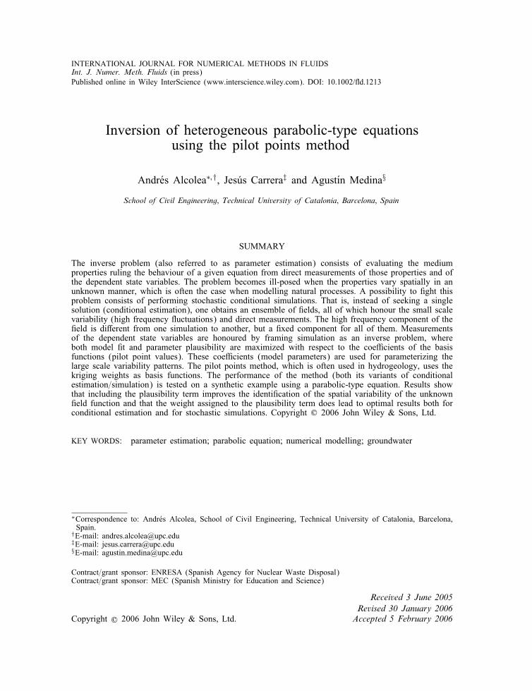
INTERNATIONAL JOURNAL FOR NUMERICAL METHODS IN FLUIDS Int. J. Numer. Meth. Fluids (in press) Published online in Wiley InterScience (www.interscience.wiley.com). DOI: 10.1002/d.1213 Inversion of heterogeneous parabolic-type equations using the pilot points method Andr es Alcolea ∗; † , Jes us Carrera ‡ and Agust n Medina § School of Civil Engineering; Technical University of Catalonia; Barcelona; Spain SUMMARY The inverse problem (also referred to as parameter estimation) consists of evaluating the medium properties ruling the behaviour of a given equation from direct measurements of those properties and of the dependent state variables. The problem becomes ill-posed when the properties vary spatially in an unknown manner, which is often the case when modelling natural processes. A possibility to ght this problem consists of performing stochastic conditional simulations. That is, instead of seeking a single solution (conditional estimation), one obtains an ensemble of elds, all of which honour the small scale variability (high frequency uctuations) and direct measurements. The high frequency component of the eld is dierent from one simulation to another, but a xed component for all of them. Measurements of the dependent state variables are honoured by framing simulation as an inverse problem, where both model t and parameter plausibility are maximized with respect to the coecients of the basis functions (pilot point values). These coecients (model parameters) are used for parameterizing the large scale variability patterns. The pilot points method, which is often used in hydrogeology, uses the kriging weights as basis functions. The performance of the method (both its variants of conditional estimation= simulation) is tested on a synthetic example using a parabolic-type equation. Results show that including the plausibility term improves the identication of the spatial variability of the unknown eld function and that the weight assigned to the plausibility term does lead to optimal results both for conditional estimation and for stochastic simulations. Copyright ? 2006 John Wiley & Sons, Ltd. KEY WORDS: parameter estimation; parabolic equation; numerical modelling; groundwater ∗ Correspondence to: Andr es Alcolea, School of Civil Engineering, Technical University of Catalonia, Barcelona, Spain. † E-mail: [email protected] ‡ E-mail: [email protected] § E-mail: [email protected] Contract=grant sponsor: ENRESA (Spanish Agency for Nuclear Waste Disposal) Contract=grant sponsor: MEC (Spanish Ministry for Education and Science) Received 3 June 2005 Revised 30 January 2006 Copyright ? 2006 John Wiley & Sons, Ltd. Accepted 5 February 2006
Transcript of Inversion of heterogeneous parabolic-type equations using the pilot points method
INTERNATIONAL JOURNAL FOR NUMERICAL METHODS IN FLUIDSInt. J. Numer. Meth. Fluids (in press)Published online in Wiley InterScience (www.interscience.wiley.com). DOI: 10.1002/�d.1213
Inversion of heterogeneous parabolic-type equationsusing the pilot points method
Andr�es Alcolea∗;†, Jes�us Carrera‡ and Agust��n Medina§
School of Civil Engineering; Technical University of Catalonia; Barcelona; Spain
SUMMARY
The inverse problem (also referred to as parameter estimation) consists of evaluating the mediumproperties ruling the behaviour of a given equation from direct measurements of those properties and ofthe dependent state variables. The problem becomes ill-posed when the properties vary spatially in anunknown manner, which is often the case when modelling natural processes. A possibility to �ght thisproblem consists of performing stochastic conditional simulations. That is, instead of seeking a singlesolution (conditional estimation), one obtains an ensemble of �elds, all of which honour the small scalevariability (high frequency �uctuations) and direct measurements. The high frequency component of the�eld is di�erent from one simulation to another, but a �xed component for all of them. Measurementsof the dependent state variables are honoured by framing simulation as an inverse problem, whereboth model �t and parameter plausibility are maximized with respect to the coe�cients of the basisfunctions (pilot point values). These coe�cients (model parameters) are used for parameterizing thelarge scale variability patterns. The pilot points method, which is often used in hydrogeology, uses thekriging weights as basis functions. The performance of the method (both its variants of conditionalestimation=simulation) is tested on a synthetic example using a parabolic-type equation. Results showthat including the plausibility term improves the identi�cation of the spatial variability of the unknown�eld function and that the weight assigned to the plausibility term does lead to optimal results both forconditional estimation and for stochastic simulations. Copyright ? 2006 John Wiley & Sons, Ltd.
KEY WORDS: parameter estimation; parabolic equation; numerical modelling; groundwater
∗Correspondence to: Andr�es Alcolea, School of Civil Engineering, Technical University of Catalonia, Barcelona,Spain.
†E-mail: [email protected]‡E-mail: [email protected]§E-mail: [email protected]
Contract=grant sponsor: ENRESA (Spanish Agency for Nuclear Waste Disposal)Contract=grant sponsor: MEC (Spanish Ministry for Education and Science)
Received 3 June 2005Revised 30 January 2006
Copyright ? 2006 John Wiley & Sons, Ltd. Accepted 5 February 2006
A. ALCOLEA, J. CARRERA AND A. MEDINA
INTRODUCTION
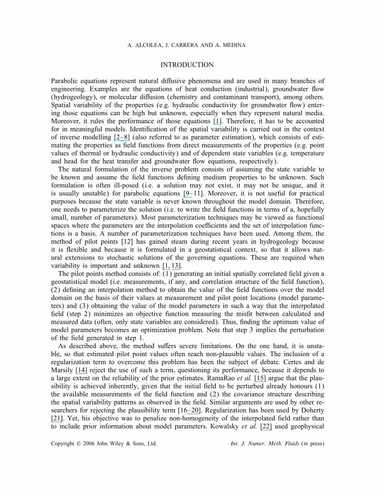
Parabolic equations represent natural di�usive phenomena and are used in many branches ofengineering. Examples are the equations of heat conduction (industrial), groundwater �ow(hydrogeology), or molecular di�usion (chemistry and contaminant transport), among others.Spatial variability of the properties (e.g. hydraulic conductivity for groundwater �ow) enter-ing those equations can be high but unknown, especially when they represent natural media.Moreover, it rules the performance of those equations [1]. Therefore, it has to be accountedfor in meaningful models. Identi�cation of the spatial variability is carried out in the contextof inverse modelling [2–8] (also referred to as parameter estimation), which consists of esti-mating the properties as �eld functions from direct measurements of the properties (e.g. pointvalues of thermal or hydraulic conductivity) and of dependent state variables (e.g. temperatureand head for the heat transfer and groundwater �ow equations, respectively).The natural formulation of the inverse problem consists of assuming the state variable to
be known and assume the �eld functions de�ning medium properties to be unknown. Suchformulation is often ill-posed (i.e. a solution may not exist, it may not be unique, and itis usually unstable) for parabolic equations [9–11]. Moreover, it is not useful for practicalpurposes because the state variable is never known throughout the model domain. Therefore,one needs to parameterize the solution (i.e. to write the �eld functions in terms of a, hopefullysmall, number of parameters). Most parameterization techniques may be viewed as functionalspaces where the parameters are the interpolation coe�cients and the set of interpolation func-tions is a basis. A number of parameterization techniques have been used. Among them, themethod of pilot points [12] has gained steam during recent years in hydrogeology becauseit is �exible and because it is formulated in a geostatistical context, so that it allows nat-ural extensions to stochastic solutions of the governing equations. These are required whenvariability is important and unknown [1, 13].The pilot points method consists of: (1) generating an initial spatially correlated �eld given a
geostatistical model (i.e. measurements, if any, and correlation structure of the �eld function),(2) de�ning an interpolation method to obtain the value of the �eld functions over the modeldomain on the basis of their values at measurement and pilot point locations (model parame-ters) and (3) obtaining the value of the model parameters in such a way that the interpolated�eld (step 2) minimizes an objective function measuring the mis�t between calculated andmeasured data (often, only state variables are considered). Thus, �nding the optimum value ofmodel parameters becomes an optimization problem. Note that step 3 implies the perturbationof the �eld generated in step 1.As described above, the method su�ers severe limitations. On the one hand, it is unsta-
ble, so that estimated pilot point values often reach non-plausible values. The inclusion of aregularization term to overcome this problem has been the subject of debate. Certes and deMarsily [14] reject the use of such a term, questioning its performance, because it depends toa large extent on the reliability of the prior estimates. RamaRao et al. [15] argue that the plau-sibility is achieved inherently, given that the initial �eld to be perturbed already honours (1)the available measurements of the �eld function and (2) the covariance structure describingthe spatial variability patterns as observed in the �eld. Similar arguments are used by other re-searchers for rejecting the plausibility term [16–20]. Regularization has been used by Doherty[21]. Yet, his objective was to penalize non-homogeneity of the interpolated �eld rather thanto include prior information about model parameters. Kowalsky et al. [22] used geophysical
Copyright ? 2006 John Wiley & Sons, Ltd. Int. J. Numer. Meth. Fluids (in press)
HETEROGENEOUS PARABOLIC-TYPE EQUATIONS
measurements (Ground Penetrating Radar) in a maximum a posteriori geostatistical context.Recently, Alcolea et al. [23] proposed adding a plausibility term to the objective function, soas to penalize departures of pilot point values from their prior estimates obtained by kriging.They showed that the use of such a regularization term improves (1) the identi�cation ofspatial variability and (2) the stability of the problem, allowing the use of larger numberof pilot points, thus sharpening the resolution of the spatial variability. However, they alsofound that including the plausibility term may lead to worse results than simply interpolatingfrom measurements (i.e. not inverting at all) if the plausibility term is not properly weighted.Fortunately, the use of a maximum likelihood statistical framework allows the identi�cationof the optimum weight of the plausibility term.A second limitation of the pilot points method is related to the de�nition of the initial spa-
tially correlated �eld: the original method of de Marsily obtained this �eld through conditionalestimation (variants of kriging [24, 25]). This yields a single ‘best’ solution that minimizesthe �eld variance and honours the available measurements of the �eld function. However, theresulting �eld is oversmoothed and does not allow a realistic representation of spatial vari-ability. To overcome this problem, some authors [15–17, 26] included conditional simulationsin the generation of the initial �eld, yielding a set of equally probable realizations of the �eldfunctions conditioned to available measurements. That is, each of these simulations reproducesthe expected variability and honours measurements. Therefore, they can be used to evaluatethe uncertainty of predictions. Unfortunately, these methods do not allow the inclusion of aplausibility term, so that they are essentially unstable.The objective of this paper is to overcome the above limitations. Speci�cally, we seek a
formulation of the inverse problem capable of generating equally probable simulations of the�eld functions (e.g. transmissivity �eld) that are conditioned to measurements of the mediumproperties and the state variables (e.g. heads). To this end, we extend the method of Alcoleaet al. [23] to the case of conditional simulation. That is, we explore the possibility of using aregularization term in the case of seeking stochastic simulations of the properties conditionedupon point measurements of both those properties and dependent state variables.This paper is organized as follows. First, the methodology is outlined. Second, a synthetic
example using the parabolic groundwater �ow equation is presented. The paper ends with adiscussion of the results and some conclusions about the use of the plausibility term in thecontext of the pilot points method.
METHODOLOGY
The proposed method is a modi�cation of the pilot points method. Modi�cations include theuse of a plausibility term and the way the vector of model parameters (value of the �eldfunctions at the pilot point locations) is updated through the optimization process. We assumethat the (geostatistical) characteristics of the �eld functions are known. Here, the geostatisticalmodel is de�ned by an autocorrelation function, but more sophisticated models may be used torepresent complex heterogeneity patterns, geophysical data or known features. The procedurecan be summarized as follows.
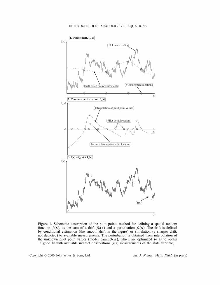
1. Parameterization: A �eld function f is expressed as the superposition of two �elds: aknown drift fD(x; t) and an uncertain residual fp(x), which is a linear combination of the
Copyright ? 2006 John Wiley & Sons, Ltd. Int. J. Numer. Meth. Fluids (in press)
A. ALCOLEA, J. CARRERA AND A. MEDINA
model parameters pj (Figure 1)
f(x; t)=fD(x; t) + fp(x) (1)
1.1. Calculation of fD(x; t): The drift can be obtained through conditional estimation(kriging=cokriging) or conditional simulation, depending on whether the modeller is seekingthe characterization of large scale patterns or small scale variability, respectively. Therefore,it honours hard data (i.e. direct measurements of the �eld function f∗) and possibly soft datag∗ (correlated with f), that can be included as external drifts. In the case of conditional sim-ulation, fD(x; t) reproduces the spatial variability patterns as observed in the �eld (honoursthe correlation structure as well), if the geostatistical model de�ned previously is informativeenough. For the simple case of linear interpolation, it can be expressed as
fD(x; t)=dim Z∑i=1�Zi (x)Z(xi ; t) (2)
where x is the location where fD is calculated, t and xi are the measurement times andlocations, respectively, and �Zj are the (co-) kriging weights for the measurements [25],organized in the vector Z=(f∗; g∗). Our implementation of the methodology allows a largeset of conditional estimation=simulation methods: simple kriging, residual kriging, krigingwith locally varying mean, kriging with external drift, simple cokriging, ordinary cokriging,ordinary cokriging (standardized to the mean value of the primary variable f), among themethods for conditional estimation [24], plus a sequential simulation algorithm for conditionalsimulations [27].1.2. Parameterization of the uncertain residual fp(x): It can be viewed as the perturbation
that the drift requires to honour measurements of dependent state variables. It is expressed asa linear combination of the model parameters (value of the �eld function at the pilot pointlocations)
fp(x)=Np∑j=1�ppj (x)pj (3)
where Np is the number of pilot points used to parameterize fp(x) (this number does not needto be the same for all �eld functions representing properties) and �ppj (x) are the (co-) krigingweights for the model parameters pj, calculated in the same way as �Zi for measurements.In our implementation, the location of the pilot points can be �xed or vary randomly as theoptimization process proceeds.2. Prior estimation: Prior estimates of the pilot point values p∗ and the corresponding
a priori error covariance matrix Vp are obtained by conditional estimation=simulation to mea-surements in vector Z. Note that correlation is included during the estimation process. In fact,pilot point values should be close (i.e. highly correlated) when pilot point locations are close.Therefore Vp is a full matrix.3. Objective function: Using maximum likelihood estimation [28], the optimum set of model
parameters minimize the objective function
F =nstat∑i=1�i(ui − u∗
i )tV−1ui (ui − u∗
i ) +ntypar∑j=1
�j(pj − p∗j )tV−1pj (pj − p∗
j ) (4)
Copyright ? 2006 John Wiley & Sons, Ltd. Int. J. Numer. Meth. Fluids (in press)
HETEROGENEOUS PARABOLIC-TYPE EQUATIONS
x
f(x)1. Define drift, fD(x)
Drift based on measurements
Unknown reality
Measurement locations
x
fp(x)2. Compute perturbation, fp(x)
0
Pilot point locations
Perturbation at pilot point location
Interpolation of pilot point values
x
f(x)3. f(x) = fD(x) + fp(x)
f(x)
Figure 1. Schematic description of the pilot points method for de�ning a spatial randomfunction f(x), as the sum of a drift fD(x) and a perturbation fp(x). The drift is de�nedby conditional estimation (the smooth drift in the �gure) or simulation (a sharper drift;not depicted) to available measurements. The perturbation is obtained from interpolation ofthe unknown pilot point values (model parameters), which are optimized so as to obtaina good �t with available indirect observations (e.g. measurements of the state variable).
Copyright ? 2006 John Wiley & Sons, Ltd. Int. J. Numer. Meth. Fluids (in press)
A. ALCOLEA, J. CARRERA AND A. MEDINA
where ‘nstat’ denotes number of state variables ui with available measurements u∗i (i.e. in
groundwater, i=1 for heads=drawdowns, i=2 for concentrations, etc.); ‘ntypar’ is the numberof types of model parameters being optimized, with prior information p∗
j (i.e. j=1 for pilotpoints linked to transmissivities, j=2 for storativities, etc.). Matrices Vui and Vpj representour best guess of the error covariance matrices of state variables and models parameters,respectively, and �i, �j are weighting scalars correcting errors in the speci�cation of Vui andVpj . In our synthetic example, we solve the groundwater �ow equation using only drawdowndata as state variable for identifying the spatial variability of the transmissivity �eld. Thus,we will term hereinafter Fd the term of state variables and Fp the term of model parameters.Assuming that error covariance matrix of drawdown is correct (�1 = 1), the simpli�ed objectivefunction can be written as
F =Fd + �Fp=(s − s∗)tV−1s (s − s∗) + �(p− p∗)tV−1
p (p− p∗) (5)
While the objective function stated in Equation (4) (or its particularization in (5)) was orig-inally based on favouring the best match of state variables (Fd), while ensuring stabilityand plausibility of the model parameters (Fp), it can also be derived in a statistical frame-work. Gavalas et al. [29] derived it by maximizing the posterior pdf (probability densityfunction) of the model parameters, MAP, while Carrera and Neuman [9] arrived to it bymaximizing the likelihood of the parameters given the data, MLE. Instead, Medina andCarrera [28] prefer working with the expected value of the likelihood function, as it al-lows the most stable estimation of statistical parameters, i.e. �i and �j. Here, we use thesame formulation.4. Minimization: The minimization of Equation (4) is performed by means of Levenberg–
Marquardt’s method. This method belongs to the Gauss–Newton family and it consists oflinearizing the dependence of state variables on model parameters, while imposing that theparameter change �pk at the kth iteration is constrained.This leads to a linear system of equations [30–32]
(Hk + �kI)�pk =−gk (6)
where Hk is an approximation of the Hessian matrix of F (Equation (4)) and gk its gradientat pk (vector of model parameters at iteration k), I is the identity matrix and �k is a positivescalar (the so-called Marquardt’s parameter).When the objective function takes a form similar to Equation (5), second-order derivatives
of the state variable with respect to the parameters are often neglected, and the approximationof the Hessian matrix can be written as
Hk =2JtsV−1s Js + 2�V
−1p (7)
where Js is the jacobian matrix (i.e. derivatives of drawdowns with respect to modelparameters at iteration k). The latter can be calculated by direct derivation of the PDE orby the adjoint state method [33]. The gradient of the objective function can bewritten as
gk =2JtsV−1s (s − s∗) + 2�V−1
p (p− p∗) (8)
Copyright ? 2006 John Wiley & Sons, Ltd. Int. J. Numer. Meth. Fluids (in press)
HETEROGENEOUS PARABOLIC-TYPE EQUATIONS
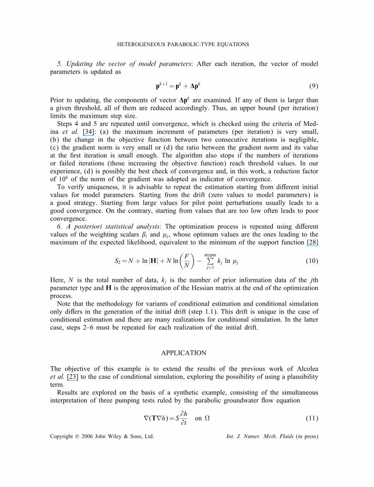
5. Updating the vector of model parameters: After each iteration, the vector of modelparameters is updated as
pk+1 = pk + �pk (9)
Prior to updating, the components of vector �pk are examined. If any of them is larger thana given threshold, all of them are reduced accordingly. Thus, an upper bound (per iteration)limits the maximum step size.Steps 4 and 5 are repeated until convergence, which is checked using the criteria of Med-
ina et al. [34]: (a) the maximum increment of parameters (per iteration) is very small,(b) the change in the objective function between two consecutive iterations is negligible,(c) the gradient norm is very small or (d) the ratio between the gradient norm and its valueat the �rst iteration is small enough. The algorithm also stops if the numbers of iterationsor failed iterations (those increasing the objective function) reach threshold values. In ourexperience, (d) is possibly the best check of convergence and, in this work, a reduction factorof 106 of the norm of the gradient was adopted as indicator of convergence.To verify uniqueness, it is advisable to repeat the estimation starting from di�erent initial
values for model parameters. Starting from the drift (zero values to model parameters) isa good strategy. Starting from large values for pilot point perturbations usually leads to agood convergence. On the contrary, starting from values that are too low often leads to poorconvergence.6. A posteriori statistical analysis: The optimization process is repeated using di�erent
values of the weighting scalars �i and �j, whose optimum values are the ones leading to themaximum of the expected likelihood, equivalent to the minimum of the support function [28]
S2 =N + ln |H|+ N ln(FN
)−
ntypar∑j=1
kj ln �j (10)
Here, N is the total number of data, kj is the number of prior information data of the jthparameter type and H is the approximation of the Hessian matrix at the end of the optimizationprocess.Note that the methodology for variants of conditional estimation and conditional simulation
only di�ers in the generation of the initial drift (step 1.1). This drift is unique in the case ofconditional estimation and there are many realizations for conditional simulation. In the lattercase, steps 2–6 must be repeated for each realization of the initial drift.
APPLICATION
The objective of this example is to extend the results of the previous work of Alcoleaet al. [23] to the case of conditional simulation, exploring the possibility of using a plausibilityterm.Results are explored on the basis of a synthetic example, consisting of the simultaneous
interpretation of three pumping tests ruled by the parabolic groundwater �ow equation
∇(T∇h)= S @h@t
on � (11)
Copyright ? 2006 John Wiley & Sons, Ltd. Int. J. Numer. Meth. Fluids (in press)

A. ALCOLEA, J. CARRERA AND A. MEDINA
where � is the �ow domain, T is the transmissivity tensor, S is storativity and h is head (thestate variable). Initial and boundary conditions can be written as
h(t=0)= h0(x) on �
T∇hn= �(H − h) +Q on �(12)
where � denotes the boundary of the �ow domain, n is a unit vector normal to � andpointing outwards, H and Q are prescribed heads and �ows, respectively, and � is a coe�cientcontrolling the type of boundary condition (�=0 for prescribed �ow, �→ ∞ for prescribedhead and a mixed condition otherwise). When pumping tests are interpreted, it is useful towork with drawdowns (di�erence between head in presence of pumping and head in absenceof pumping), denoted as ‘s’ hereinafter. This leads to homogeneous (zero) initial and boundarydrawdowns, as well as boundary �ow rates. Equation (11) is solved applying the Galerkinmethod in space and forward �nite di�erences in time. Elements are quadrangular bilinear.The �ow domain is a square of 400× 400m2, despite it is enlarged to avoid spurious
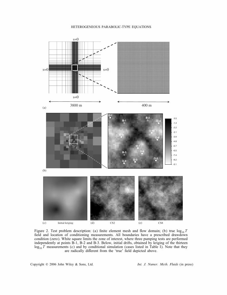
boundary e�ects to a global domain of 3600× 3600m2 (Figure 2(a)). The �nite element gridis more re�ned in the central part (zone of interest, Figure 2). There, the �nite element meshis structured. Outside, the element size increases as the mesh progresses towards the boundarydomain (Figure 2(a)).The ‘true’ log transmissivity �eld (log10 T hereinafter) was generated with the code
TRANSIN [34] by sequential simulation (Figure 2(a)) conditional to a set of measurementsde�ning two channels of high transmissivity. The ‘true’ variogram (�eld variance minusautocorrelation function) is spherical, with a range of 200m and a variance of 2, withoutnugget e�ect. Values of the ‘true’ log10 T �eld range from −9:1 to 0.5, with a mean valueof −4[log10(m2=s)]. In this work, only the heterogeneity of the log10 T �eld was explored.Storativity was assumed to be constant and known over the whole domain, with a valueof 10−4.Thirteen measurements of log10 T were selected from the ‘true’ �eld as conditioning data.
Measurement locations were purposefully selected in such a way that the initial drift ofEquation (2) (calculated by ordinary kriging or by sequential simulation, for the cases ofconditional estimation=simulation, respectively) was radically di�erent from the ‘true’ �eld(Figure 2(b)). Note that, indeed, the high log10 T channels crossing the zone of interest aremissed by the drift. Thus, the performance of the model is heavily dependent on the calibrationof the perturbation �eld fp. This setup was chosen to ensure that the plausibility term, whichbiases the solution towards the drift, would hinder �nding a good solution.Drawdown data comes from three independent pumping tests (but analysed simultaneously)
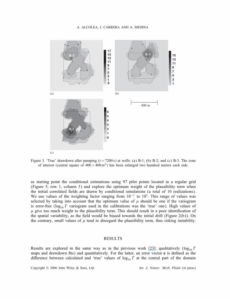
in the most productive wells of the central domain (pumping rates of 10−2 m3=s at wells B1,B2 and B3 in Figure 2). Transient drawdowns were simulated at grid nodes (Figure 3),assuming a zero drawdown as initial condition and prescribed at the boundaries of the globaldomain. Drawdown measurements were calculated at the thirteen points where log10 T mea-surements are available (total of 936 drawdown data). A Gaussian white noise was addedto those measurements, simulating acquisition errors, with a standard deviation of 0.3m forpumping at wells B1 and B2 and 0.15m at well B3 (1% of the maximum drawdown at eachone of the tests).In the previous work of Alcolea et al. [23], the optimum weight of the plausibility term
was found for the case of conditional estimation. For the purpose of this paper, we take
Copyright ? 2006 John Wiley & Sons, Ltd. Int. J. Numer. Meth. Fluids (in press)
HETEROGENEOUS PARABOLIC-TYPE EQUATIONS
B-1
B-2
B-3
O-1
O-2
O-3O-4O-5
O-6
O-7
O-8O-9
O-10
s=0
s=0
s=0 s=0
3800 m 400 m (a)
(b)
(c) Initial kriging CS2 CS8(d) (e)
-9.1
-8.2
-7.4
-6.5
-5.7
-4.8
-3.9
-3.1
-2.2
-1.4
0.5
Figure 2. Test problem description: (a) �nite element mesh and �ow domain; (b) true log10 T�eld and location of conditioning measurements. All boundaries have a prescribed drawdowncondition (zero). White square limits the zone of interest, where three pumping tests are performedindependently at points B-1, B-2 and B-3. Below, initial drifts, obtained by kriging of the thirteenlog10 T measurements (c) and by conditional simulation (cases listed in Table I). Note that they
are radically di�erent from the ‘true’ �eld depicted above.
Copyright ? 2006 John Wiley & Sons, Ltd. Int. J. Numer. Meth. Fluids (in press)
A. ALCOLEA, J. CARRERA AND A. MEDINA
B-1
1357911131517
0
B-2
13579111315
B-3
0123456
(a) (b)
(c)
400 m
Figure 3. ‘True’ drawdown after pumping (t=7200 s) at wells: (a) B-1; (b) B-2; and (c) B-3. The zoneof interest (central square of 400× 400m2) has been enlarged two hundred meters each side.
as starting point the conditional estimations using 97 pilot points located in a regular grid(Figure 5; row 1, column 3) and explore the optimum weight of the plausibility term whenthe initial correlated �elds are drawn by conditional simulations (a total of 10 realizations).We use values of the weighting factor ranging from 10−1 to 102. This range of values wasselected by taking into account that the optimum value of � should be one if the variogramis error-free (log10 T variogram used in the calibrations was the ‘true’ one). High values of� give too much weight to the plausibility term. This should result in a poor identi�cation ofthe spatial variability, as the �eld would be biased towards the initial drift (Figure 2(b)). Onthe contrary, small values of � tend to disregard the plausibility term, thus risking instability.
RESULTS
Results are explored in the same way as in the previous work [23]: qualitatively (log10 Tmaps and drawdown �ts) and quantitatively. For the latter, an error vector e is de�ned as thedi�erence between calculated and ‘true’ values of log10 T at the central part of the domain
Copyright ? 2006 John Wiley & Sons, Ltd. Int. J. Numer. Meth. Fluids (in press)
HETEROGENEOUS PARABOLIC-TYPE EQUATIONS
(1600 blocks of 10× 10m2). We analyse the following statistics:(1) Total objective function and its drawdowns and parameters components (F , Fd and Fp
in Equation (5), respectively). These are not good comparison criteria as they grow(F and Fd) or decrease monotonically (Fp) with �.
(2) Support function of the expected likelihood (Equation (10)), whose minimization shouldlead to the optimum value of �.
(3) Mean error: measures the match between calculated and ‘true’ values of log10 T
elog10 T =11600
1600∑i=1
|ei|= 11600
1600∑i=1
| log10 T calc − log10 T true| (13)
We used this criterion rather than the raw one measuring the estimation bias (identicalbut without absolute value), given that the latter, also evaluated, was close to zero inmost cases, as expected. Therefore, it did not shed new light on this research.
(4) Root mean square error of log10 T : this is the basic raw criterion to evaluate the good-ness of the identi�cation. Theoretically, it should be smaller than the a priori deviation(square root of the variogram sill,
√2 in this case), if conditioning is good
RMSElog10 T =(
11600
ete)1=2
(14)
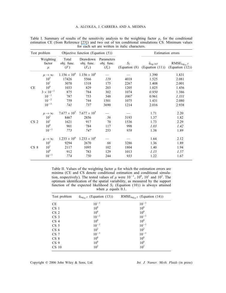
As will be discussed later, mean error and root mean square error are very sensitive to thelocation and extreme values of the zones of high=low transmissivity.Table I displays a comparison between the evolution of the statistics with the weight of
the plausibility term for the conditional estimation and two out of ten conditional simulations.Table II summarizes the quantitative comparisons and contains the value of � for which the es-timation statistics reach their optimum value. For instance, the minimum value of RMSElog10 Tis attained at �=0:1 in simulation 5. Figure 4 displays the quantitative comparison in termsof the support function of the expected likelihood S2 and the estimation errors, elog10 T andRMSElog10 T . Identi�cations of log10 T are presented in Figure 5. Figure 6 displays the bestmatching of drawdown.The �rst observation that becomes apparent from Table I is the strong e�ect of the de-
pendence of the plausibility term, as occurred in the previous work. The relative importancegiven to this term is measured by the value of the weighting factor �. Using small val-ues for this factor (little importance of the plausibility term, disregarding prior estimates inthe optimization process and therefore, prior information) consistently leads to the best �tof drawdowns (minimum value of Fd) and to the worst �t of model parameters (maximumvalue of Fp), as expected. Identi�cations of the spatial variability (Figure 5; last row, column2) using a weighting factor of 10−1 o�er a somewhat ‘lumpy’ appearance, with large jumpsin the calibrated transmissivity over small distances. In fact, when the drift is generated byconditional estimation, Alcolea et al. [23] found the optimum identi�cation when � equals0.1 (the minimum value tested in this example), that yields the worst qualitative identi�cationof the log10 T �eld in this work. In fact, values of � lower than 10−1 were excluded fromthis study due to instability problems.Similarly, large values of the weighting factor also yield poor results. The �nal solution
tends to be close to the initial drift (Figure 5, �rst row), which contains little information
Copyright ? 2006 John Wiley & Sons, Ltd. Int. J. Numer. Meth. Fluids (in press)
A. ALCOLEA, J. CARRERA AND A. MEDINA
Table I. Summary of results of the sensitivity analysis to the weighting factor �, for the conditionalestimation CE (from Reference [23]) and two out of ten conditional simulations CS. Minimum values
for each set are written in italic characters.
Test problem Objective function (Equation (5)) Estimation errors
Weighting Total Drawdown Parametersfactor obj. func. obj. func. obj. func. S2 elog 10T RMSElog10 T� (F) (Fd) (Fp) (Equation (8) (Equation (11)) (Equation (12))
�→ ∞ 1:156× 106 1:156× 106 — — 1.390 1.831102 17426 5566 119 4018 1.525 2.081101 3070 1318 175 2267 1.408 2.001
CE 100 1033 829 203 1205 1.025 1.4563× 10⁻¹ 875 784 302 1074 0.950 1.38610−1 787 753 348 1007 0.961 1.33110−2 759 744 1501 1075 1.431 2.08010−3 741 737 3690 1214 2.016 2.938
�→ ∞ 7:677× 105 7:677× 105 — — 1.71 2.20102 8467 2856 56 3193 1.37 1.82
CS 2 101 1621 917 70 1536 1.73 2.29100 901 784 117 998 1.03 1.4210−1 773 747 253 958 1.38 1.89
�→ ∞ 1:233× 106 1:233× 106 — — 1.64 2.12102 9294 2670 66 3286 1.36 1.89
CS 8 101 2117 1095 102 1804 1.40 1.94100 912 783 129 1013 1.15 1.5710−1 774 750 244 933 1.22 1.67
Table II. Values of the weighting factor � for which the estimation errors areminima (CE and CS denote conditional estimation and conditional simula-tion, respectively). The tested values of � were 10−1, 100, 101 and 102. Theoptimum identi�cation of the spatial variability, as measured by the supportfunction of the expected likelihood S2 (Equation (10)) is always attained
when � equals 0.1.
Test problem elog10 T (Equation (13)) RMSElog10 T (Equation (14))
CE 10−1 10−1
CS 1 100 100
CS 2 100 100
CS 3 10−1 10−1
CS 4 100 100
CS 5 10−1 10−1
CS 6 102 102
CS 7 10−1 10−1
CS 8 100 100
CS 9 100 100
CS 10 102 102
Copyright ? 2006 John Wiley & Sons, Ltd. Int. J. Numer. Meth. Fluids (in press)
HETEROGENEOUS PARABOLIC-TYPE EQUATIONS
0.1 1 10 100µ µ
µ
1000
2000
3000
4000
5000
Sup
port
func
tion
of th
e ex
pect
ed li
kelih
ood
S2
(a) (b)
(c)
0.1 1 10 100
0.5
1
1.5
2
2.5
3
Mea
n er
ror
e
0.1 1 10 100
1
2
3
4
Roo
t mea
n sq
uare
err
or R
MS
E
ECSC1SC2
SC3SC4SC5SC6SC7SC8
SC9SC10
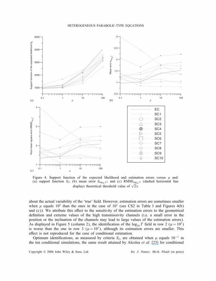
Figure 4. Support function of the expected likelihood and estimation errors versus � and:(a) support function S2; (b) mean error elog10 T ; and (c) RMSElog10 T (dashed horizontal line
displays theoretical threshold value of√2).
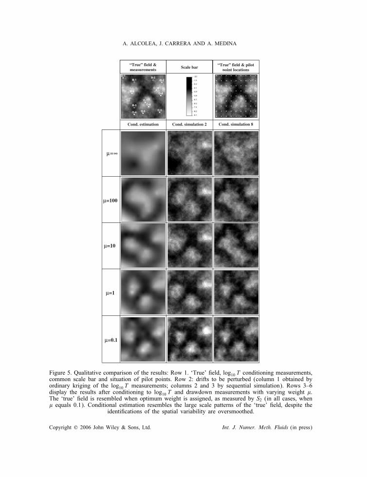
about the actual variability of the ‘true’ �eld. However, estimation errors are sometimes smallerwhen � equals 102 than the ones in the case of 101 (see CS2 in Table I and Figures 4(b)and (c)). We attribute this e�ect to the sensitivity of the estimation errors to the geometricalde�nition and extreme values of the high transmissivity channels (i.e. a small error in theposition or the inclination of the channels may lead to large values of the estimation errors).As displayed in Figure 5 (column 2), the identi�cation of the log10 T �eld in row 2 (�=10
2)is worse than the one in row 3 (�=101), although its estimation errors are smaller. Thise�ect is not reproduced for the case of conditional estimation.Optimum identi�cations, as measured by criteria S2, are obtained when � equals 10−1 in
the ten conditional simulations, the same result attained by Alcolea et al. [23] for conditional
Copyright ? 2006 John Wiley & Sons, Ltd. Int. J. Numer. Meth. Fluids (in press)
A. ALCOLEA, J. CARRERA AND A. MEDINA
µ=µ=∞
µ=10
µ=1
µ=100
µ=0.1
Cond. estimation
“True” field & measurements
Cond. simulation 2 Cond. simulation 8
“True” field & pilot point locations
Scale bar
B-1B-2
B-3
O-1
O-2
O-3O-4O-5
O-6
O-7
O-8O-9
O-10
Figure 5. Qualitative comparison of the results: Row 1. ‘True’ �eld, log10 T conditioning measurements,common scale bar and situation of pilot points. Row 2: drifts to be perturbed (column 1 obtained byordinary kriging of the log10 T measurements; columns 2 and 3 by sequential simulation). Rows 3–6display the results after conditioning to log10 T and drawdown measurements with varying weight �.The ‘true’ �eld is resembled when optimum weight is assigned, as measured by S2 (in all cases, when� equals 0.1). Conditional estimation resembles the large scale patterns of the ‘true’ �eld, despite the
identi�cations of the spatial variability are oversmoothed.
Copyright ? 2006 John Wiley & Sons, Ltd. Int. J. Numer. Meth. Fluids (in press)
HETEROGENEOUS PARABOLIC-TYPE EQUATIONS
B-1B-2
B-3
O-1
O-2
O-3O-4O-5
O-6
O-7
O-8O-9
O-10
0 6000 12000 18000 24000 30000 36000
0.1
1
10Observation point O-10
24000 320001
10
0 6000 12000 18000 24000 30000 36000
0.1
1
10
Measured drawdownConditional EstimationConditional simulation 2Conditional simulation 8
Measured drawdownConditional EstimationConditional simulation 2Conditional simulation 8
Measured drawdownConditional EstimationConditional simulation 2Conditional simulation 8
Measured drawdownConditional EstimationConditional simulation 2Conditional simulation 8
Observation point B-2
0 800 1600
0.1
1
0.1
1
10Observation point O-8
0 800 1600
0.1
1
0 6000 12000 18000 24000 30000 36000
0.1
1
10Observation point O-5
0 800 1600
0.1
1
Time (s)
Dra
wdo
wn
(m)
Time (s)
Time (s) 0 6000 12000 18000 24000 30000 36000
Time (s)
Dra
wdo
wn
(m)
Dra
wdo
wn
(m)
Dra
wdo
wn
(m)
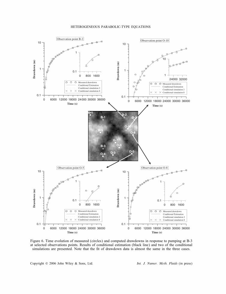
Figure 6. Time evolution of measured (circles) and computed drawdowns in response to pumping at B-3at selected observations points. Results of conditional estimation (black line) and two of the conditionalsimulations are presented. Note that the �t of drawdown data is almost the same in the three cases.
Copyright ? 2006 John Wiley & Sons, Ltd. Int. J. Numer. Meth. Fluids (in press)
A. ALCOLEA, J. CARRERA AND A. MEDINA
estimation. This is important because it suggests that the modeller does not need to identifythe optimum weight for each conditional simulation (usually a large number), but to obtainit just once using the method in its variant of conditional estimation.Another result shared by conditional estimation and simulation is that, if the plausibility term
is not properly weighted, the identi�cation of the spatial variability is worse than the initialdrift, as measured by estimation errors (Table I). However, the use of the methodology in amaximum likelihood framework allows the estimation of the weighting factor �. Therefore,the use of a plausibility term is advisable, independently of how the drift was calculated.Figure 6 displays the best drawdown �t (� equals 0.1) for the conditional simulations at
Table I and the conditional estimation. Calculated drawdowns are very similar in all cases and�t the data. In fact, drawdown objective functions were very similar in all cases (Table I).Despite the best match to drawdown data is obtained when the plausibility term is neglected,the drawdown �ts for the optimum identi�cation of the log10 T �eld (optimum weightingscalar �) were nearly as good as the best ones (� → 0) and the simulation was stable.
CONCLUSIONS
The pilot points method provides a powerful tool for the identi�cation of the �eld functionsruling the behaviour of a PDE. The suggested approach includes a plausibility term in theoptimization process and two ways for calculating the initial drift, by conditional estimationor simulations conditioned to the direct measurements of the �eld function. Conditional esti-mation leads to optimal results (i.e. minimum estimation errors) but fails to reproduce smallscale variability, which may be important when using the model for predictions. Instead,conditional simulation seeks a set of equally likely realizations of the �eld conditioned toall available information. Both variants have been tested on a synthetic example using theparabolic groundwater �ow equation, examining the role of the plausibility term.We have found that, neglecting the plausibility term, which is the standard approach in
the context of pilot points, favours the best match of drawdown data, but often leads to anunstable identi�cation of the model parameters. Large values give too much importance tothe plausibility term, which biases the solution towards the drift. If the geostatistical modelcontains little information of the variability patterns (as in our synthetic example), the solutionyields poor identi�cations of the spatial variability. In fact, a disturbing �nding is that, inmost cases, conditioning the �elds to state variable data worsens the results if the plausibilityterm is not weighted properly. Fortunately, the use of a statistical framework (maximumlikelihood in this case) allows the estimation of the optimum weight of the plausibility term,and therefore, its use is recommended. However, to search this optimum weight for eachconditional simulation can be tedious.A key �nding of this work is that the optimum value of the weighting factor (as measured
by the support function of the expected likelihood) was the same as the one obtained usingconditional estimation. This frees the modeller of the burden of having to seek the optimumweight at each conditional simulation (usually a large number).Good �ts to measured state variable were obtained when neglecting (assigning low weight
to) prior information. Still, �ts nearly as good were obtained with stable simulations whenmoderate weights were assigned to prior information. We stress that the prior informationprovides a valuable data of aquifer heterogeneity, even when it is poorly informative of the
Copyright ? 2006 John Wiley & Sons, Ltd. Int. J. Numer. Meth. Fluids (in press)
HETEROGENEOUS PARABOLIC-TYPE EQUATIONS
actual variability. Thus, the use of a plausibility term including it (usually disregarded in thecontext of pilot points) needs to be considered.
ACKNOWLEDGEMENTS
This work was funded by ENRESA (Spanish Agency for Nuclear Waste Disposal) and MEC (SpanishMinistry for Education and Science).
REFERENCES
1. Freeze RA. A stochastic-conceptual analysis of one-dimensional groundwater �ow in nonuniform homogeneousmedia. Water Resources Research 1975; 11(5):725–741.
2. Carrera J, Alcolea A, Medina A, Hidalgo J, Slooten LJ. Inverse problem in hydrogeology. Hydrogeology Journal2004; 13(1):206–222.
3. Carrera J. State of the art of the inverse problem applied to the �ow and solute transport problems. GroundwaterFlow and Quality Modeling, NATO ASI Series 1987; 549–585.
4. Ouyang T. Analysis of parameter-estimation heat-conduction problems with phase-change using the �nite-elementmethod. International Journal for Numerical Methods in Engineering 1992; 33(10):2015–2037.
5. Schnur DS, Zabaras N. An inverse method for determining elastic-material properties and a material interface.International Journal for Numerical Methods in Engineering 1992; 33(10):2039–2057.
6. de Marsily G, Delhomme JP, Delay F, Buoro A. 40 years of inverse problems in hydrogeology. ComptesRendus de l’Academie des Sciences Series IIA Earth and Planetary Science 1999; 329(2):73–87.
7. McLaughlin D, Townley LLR. A reassessment of the groundwater inverse problem. Water Resources Research1996; 32(5):1131–1161.
8. Yeh WWG. Review of parameter estimation procedures in groundwater hydrology: the inverse problem. WaterResources Research 1986; 22(2):95–108.
9. Carrera J, Neuman SP. Estimation of aquifer parameters under transient and steady-state conditions. 1. Maximumlikelihood method incorporating prior information. Water Resources Research 1986; 22(2):199–210.
10. Carrera J, Neuman SP. Estimation of aquifer parameters under transient and steady-state conditions.2. Uniqueness, stability and solution algorithms. Water Resources Research 1986; 22(2):211–227.
11. Carrera J, Neuman SP. Estimation of aquifer parameters under transient and steady-state conditions,3. Application to synthetic and �eld data. Water Resources Research 1986; 22(2):228–242.
12. de Marsily GH, Lavedan G, Boucher M, Fasanino G. Interpretation of interference tests in a well �eld usinggeostatistical techniques to �t the permeability distribution in a reservoir model. In Geostatistics for NaturalResources Characterization. Part 2, Verly D et al. (eds). D. Reidel Publication Co.: Dordrecht, 1984; 831–849.
13. Narayanan VAB, Zabaras N. Stochastic inverse heat conduction using a spectral approach. International Journalfor Numerical Methods in Engineering 1992; 60(9):1569–1593.
14. Certes C, de Marsily GH. Application of the pilot point method to the identi�cation of aquifer transmissivities.Advances in Water Resources 1991; 14(5):284–300.
15. RamaRao BS, Lavenue M, de Marsily GH, Marietta MG. Pilot point methodology for automated calibration ofan ensemble of conditionally simulated transmissivity �elds. 1. Theory and computational experiments. WaterResources Research 1995; 31(3):475–493.
16. Capilla JE, G�omez-Hern�andez JJ, Sahuquillo A. Stochastic simulation of transmissivity �elds conditional toboth transmissivity and piezometric data. 2. Demonstration on a synthetic aquifer. Journal of Hydrology 1997;203:175–188.
17. G�omez-Hern�andez JJ, Sahuquillo A, Capilla JE. Stochastic simulation of transmissivity �elds conditional to bothtransmissivity and piezometric data. 1. Theory. Journal of Hydrology 1997; 204(1–4):162–174.
18. Lavenue M, RamaRao BS, de Marsily GH, Marietta MG. Pilot point methodology for automated calibration ofan ensemble of conditionally simulated transmissivity �elds. 2. Application. Water Resources Research 1995;31(3):495–516.
19. Lavenue M, de Marsily GH. Three-dimensional interference test interpretation in a fractured aquifer using thepilot-point inverse method. Water Resources Research 2001; 37(11):2659–2675.
20. Wen XH, Deutsch CV, Cullick AS. Construction of geostatistical aquifer models integrating dynamic �ow andtracer data using inverse technique. Journal of Hydrology 2002; 255:151–168.
21. Doherty J. Groundwater model calibration using pilot points and regularization. Ground Water 2003; 41(2):170–177.
22. Kowalsky MB, Finsterle S, Rubin Y. Estimating �ow parameter distributions using ground-penetrating radarand hydrological measurements during transient �ow in the vadose zone. Advances in Water Resources 2004;27:583–599.
Copyright ? 2006 John Wiley & Sons, Ltd. Int. J. Numer. Meth. Fluids (in press)

A. ALCOLEA, J. CARRERA AND A. MEDINA
23. Alcolea A, Carrera J, Medina A. Pilot points method incorporating prior information for solving the groundwater�ow inverse problem. Advances in Water Resources 2006, in press.
24. Gu L. Moving kriging interpolation and element-free Galerkin method. International Journal for NumericalMethods in Engineering 2003; 56(1):1–11.
25. Krige DG. A statistical approach to some mine evaluation and allied problems on the Witwatersrand. Ph.D.Thesis, University of the Witwatersrand, Johannesburg, 1951.
26. Hendricks-Franssen HJ. Inverse stochastic modelling of groundwater �ow and mass transport. Ph.D. Thesis,Technical University of Valencia, Spain, 2001.
27. Liu YH, Journel A. Improving sequential simulation with a structured path guided by information content.Mathematical Geology 2004; 36(8):945–964.
28. Medina A, Carrera J. Geostatistical inversion of coupled problems: dealing with computational burden anddi�erent types of data. Journal of Hydrology 2003; 281:251–264.
29. Gavalas GR, Shaw PC, Sein�eld JH. Reservoir history matching by Bayesian estimation. Society of PetroleumEngineers Journal 1976; 261:337–350.
30. Marquardt DW. An algorithm for least-squares estimation of non-linear parameters. Journal of the Society forIndustrial and Applied Mathematics 1963; 11(2):431–441.
31. Cooley RL. Regression modeling of groundwater �ow. USGS Open Report 1985; 85–180.32. Bereaux Y, Clermont JR. Numerical-simulation of complex �ows of non-newtonian �uids using the stream tube
method and memory integral constitutive-equations. International Journal for Numerical Methods in Fluids1995; 21(5):371–389.
33. Galarza GA, Carrera J, Medina A. Computational techniques for optimization of problems involving non-lineartransient simulations. International Journal for Numerical Methods in Engineering 1999; 45(3):319–334.
34. Medina A, Alcolea A, Carrera J, Castro LF. Modelos de �ujo y transporte en la geosfera: C�odigo Transin IV.In IV Jornadas de Investigaci�on y Desarrollo Tecnol�ogico de Gesti�on de Residuos Radiactivo de ENRESA.Publicaci�on t�ecnica 9=2000, 2000; 195–200.
Copyright ? 2006 John Wiley & Sons, Ltd. Int. J. Numer. Meth. Fluids (in press)