arX

iv:c

ond-

mat

/051

2448

v1 [

cond

-mat

.dis

-nn]

19

Dec

200

5

Bump formations in binary attractor neural network

Kostadin Koroutchev∗

Depto. de Ingenierıa InformaticaUniversidad Autonoma de Madrid,

28049 Madrid, Spain †

Elka KorutchevaDepto. de Fısica Fundamental,

Universidad Nacional de Educacion a Distancia,c/ Senda del Rey 9,28080 Madrid, Spain ‡

This paper investigates the conditions for the formation of local bumps in the activity of binaryattractor neural networks with spatially dependent connectivity. We show that these formationsare observed when asymmetry between the activity during the retrieval and learning is imposed.Analytical approximation for the order parameters is derived. The corresponding phase diagramshows a relatively large and stable region, where this effect is observed, although the critical storageand the information capacities drastically decrease inside that region. We demonstrate that thestability of the network, when starting from the bump formation, is larger than the stability whenstarting even from the whole pattern. Finally, we show a very good agreement between the analyticalresults and the simulations performed for different topologies of the network.

PACS numbers: 87.18.Sn, 64.60.Cn, 07.05.Mh

I. INTRODUCTION

The bump formations in recurrent neural networkshave been recently reported in several investigations con-cerning linear-threshold units [1, 2], binary units [3, 4],Small-World networks of Integrate and Fire neurons [5]and in a variety of spatially distributed neural networksmodels with excitatory and inhibitory couplings betweenthe cells [6, 7].

As has been shown, the localized retrieval is due tothe short-range connectivity of the networks and couldexplain the behavior in structures of biological relevanceas the neocortex, where the probability of connectionsdecreases with the distance [8].

In the case of linear-threshold neural network model,the signal-to-noise analysis has been recently adapted[1, 2] to spatially organized networks and has shown thatthe retrieval states of the connected network have non-uniform activity profiles when the connections are short-range enough, even without any spatial structure of thestored patterns. The increase of the gain or the satura-tion level of neurons enhance the level of localization ofthe retrieval states and do not lead to a drastic decreaseof the storage capacity in these networks even for verylocalized solutions [2].

An interesting investigation of the spontaneous ac-tivity bumps in Small-World networks (SW) [9, 10] ofIntegrate-and Fire neurons [5], has recently shown that

∗Electronic address: k.koroutchev@uam.es†Also at Inst. for Communications and Computer Systems, Bul-

garian Academy of Sciences, 1113, Sofia, Bulgaria‡Also at G.Nadjakov Inst.Solid State Physics, Bulgarian Academy

of Sciences, 1784 Sofia, Bulgaria

the network retrieves when its connectivity is close to therandom and displays localized bumps of activity, when itsconnectivity is close to the ordered. The two regimes aremutually exclusive in the range of the parameter gov-erning the proportion of the long-range connections onthe SW topology of Integrate-and-Fire network, whilethe two behaviors coexist in the case of linear-thresholdand smoothly saturated units. Moreover, it has beenstated that the transition between localization and re-trieval regimes, in the case of SW networks of Integrate-and-Fire neurons, can occur at a degree of randomnessbeyond the SW regime and it is not related, in general,to the SW properties of the network.

The bump formations have been also investigated inspatially distributed neural network models with excita-tory and inhibitory synaptic couplings. Recently it hasbeen shown [6] that a neural network only with excitatorycouplings can exhibit localized activity from an initialtransient synchrony of a localized group of cells, followedby desynchronized activity within the group. This activ-ity may grow or may be reduced when depression witha given size of the frequency of the inputs is introduced.It is also very sensitive to the initial conditions and therange of the parameters of the network.

The result of bump formations have been recently re-ported by us, [3, 4] in the case of binary Hebb model forassociative network. We stated out that these spatiallyasymmetric retrieval states (SAS) can be observed if anasymmetry between the learning and the retrieval statesis imposed. This means that the network is constrainedto have a different activity compared to that induced bythe patterns.

In the present investigation we regard a symmetric anddistance dependent connectivity for all neurons within anattractor neural network (NN) of Hebbian type formed by

2

N binary neurons {Si}, Si ∈ {−1, 1}, i = 1, ..., N , storingp binary patterns ηµ

i , µ ∈ {1...p}. The connectivity be-tween the neurons is symmetric cij = cji ∈ {0, 1}, cii = 0,where cij = 1 means that neurons i and j are connected.

We are interested only on connectivities in whichthe fluctuations between the individual connectivity aresmall, e.g. ∀i

∑

j cij ≈ cN , where c is the mean connec-tivity.

The learned patterns are drawn from the following dis-tribution:

P (ηµi ) =

1 + a

2δ(ηµ

i − 1) +1 − a

2δ(ηµ

i + 1),

where the parameter a is the sparsity of the code [11, 12].We study the Hopfield model [13]:

H =1

N

∑

ij

JijSiSj , (1)

with Hebbian learning rule [14]

Jij =1

c

p∑

µ=1

cij(ηµi − a)(ηµ

j − a). (2)

Further in this article we will work in terms of variablesξµi ≡ ηµ

i − a.In the case of binary network and symmetrically dis-

tributed patterns, the only asymmetry between the re-trieval and the learning states that can be imposed, in-dependent on the position of the neurons, is the totalnumber of the neurons in a given state. Having in mindthat there are only two possible states, this conditionleads to a condition on the mean activity of the network,which is introduced by adding an extra term Ha to theHamiltonian

Ha = NR(∑

i

Si/N − a).

This term favors states with lower total activity∑

i Si

that is equivalent to decrease the number of active neu-rons, creating asymmetry between the learning and theretrieval states.

For R = 0, this model has been intensively studied[11, 12, 15] and shows no evidence of spatial asymmetricstates.

For R > 0, the energy of the system increases withthe number of active neurons (Si = 1) and the term Ha

tends to limit the number of active neurons below aN .In the present work we show explicitly that the con-

straint on the network level of activity is a sufficient con-dition for observation of spatially asymmetric states inbinary Hebb neural network. Similar observations havebeen reported in the case of linear-threshold network [1],where in order to observe bump formations, one has toconstrain the activity of the network. The same is truein the case of smoothly saturating and binary networks[2], when the highest activity level, they can achieve, is

above the maximum activity of the units in the storedpattern.

In the present paper we discuss in details the bi-nary neural network model, giving a complete analyticalderivation of its properties. We explain the minimal con-ditions for the formations of spatially asymmetric statesin a recurrent network with metrically organized connec-tivity.

We compare the results for three different topologies ofthe network and show interesting multi-bump formationsin the case of the SW-like topology. Further extension ofthe analysis to the information, carried by the network,reveals that the retrieved states can be well recoveredby a limited amount of information. We show that thestability of the network’s retrieval, when starting fromthe bump, is larger than the stability, when starting evenfrom the whole pattern. This could be useful in practicalretrieval tasks with minimal information transmitted.

The paper is organized as follows: In section Analyticalanalysis and using replica theory, we present our detailedmean-field analysis in the case of distance-dependent con-nectivities. We derive the equations for the correspond-ing order parameters (OP) for finite and zero tempera-tures. In section Simulations we present the results ofthe simulations, done for the case of different topologiesof the network, and we compare them with the analyticalresults. In section Discussion we focus on the stability ofthe phase diagram of the network and especially on thedependence of the SAS region on the parameters of themodel. We discuss the behavior of the critical storage ca-pacity when bump formations are present, as well as theireffect on the information capacity of the network. Theconclusion, drawn in the last part, shows that only theasymmetry between the learning and the retrieval statesis sufficient to observe spatially asymmetric states.

II. ANALYTICAL ANALYSIS

For the analytical analysis of the SAS states, we con-sider the decomposition of the connectivity matrix cij by

its eigenvectors a(k)i :

cij =∑

k

λka(k)i a

(k)j ,

∑

i

a(k)i a

(l)i = δkl,

where λk are the corresponding (positive) eigenvalues.

For convenience we denote bki ≡ a

(k)i

√λk, having

cij =∑

k

bki bk

j .

We will assume that a(k)i are ordered by their eigenval-

ues in decreasing order, e.g. for k > l ⇒ λk ≤ λl. To get

some intuition of what a(k)j look like, we plot in Fig. 1

the first two eigenvectors.For a wide variety of connectivities, the first three

eigenvectors approximate:

a(0)k =

√

1/N, (3)

3

0 0.2 0.4 0.6 0.8 1x=i/N

−2.00

−1.00

0.00

1.00

2.00

b 0(x)

,b1(

x)

bo

b1

FIG. 1: (Color online) The components of the first and thesecond eigenvectors of the connectivity matrix for N = 6400,c = 320/N , λ1 = 319.8, λ2 = 285.4. The first eigenvector hasconstant components, the second one - sine-like components.

a(1)k =

√

2/N cos(2π|k − k0|/N) (4)

and

a(2)k =

√

2/N sin(2π|k − k0|/N). (5)

Following the classical analysis of Amit et al. [15],we use Bogolyubov’s method of quasi averages [16] to

have into account a finite numbers of overlaps that con-dense macroscopically. To this aim we introduce an ex-ternal field, conjugate to a finite number of patterns{ξν

i }, ν = 1, 2, ..., s, adding to the Hamiltonian the termHh =

∑sν=1 hν

∑

i ξνi Si.

In order to impose some asymmetry in the neu-ral network’s states, we also add the term Ha =NR (

∑

i Si/N − a).

The whole Hamiltonian, we are studying, is:

H =1

cN

∑

ijµ

Siξµi cijξ

µj Sj +

s∑

ν=1

hν∑

i

ξνi Si

+NR(∑

i

Si/N − a). (6)

By using the “replica method” [17], for the averagedfree energy per spin we get:

f = − limn→0

limN→∞

1

βnN(〈〈Zn〉〉 − 1), (7)

where 〈〈...〉〉 stands for the average over the pattern dis-tribution P (ξµ

i ), n is the number of the replicas, whichare later taken to zero and β is the inverse temperature.

The replicated partition function is

〈〈Zn〉〉 =

⟨⟨

TrSρ exp

[

β

2cN

∑

ijµρ

(ξµi Sρ

i )cij(ξµj Sρ

j ) − 1

2cβpn +

β∑

ν

hν∑

i,ρ

ξνi Sρ

i −∑

ρ

βNR(∑

i

Sρi /N − a)

]⟩⟩

. (8)

The decomposition of the sites, by using an expansion of the connectivity matrix cij over its eigenvalues λl, l = 1, ..., Mand its eigenvectors al

i, gives:

〈〈Zn〉〉 = e−βpn/2c

⟨⟨

TrSρ exp

[

β

2cN

∑

µρl

∑

ij

(ξµi Sρ

i bli)(ξ

µj Sρ

j blj) +

β∑

ν

hν∑

iρ

ξνi Sρ

i −∑

ρ

βRN(∑

i

Sρi /N − a)

]⟩⟩

. (9)

Introducing variables mµρl at each replica ρ, each configuration and each eigenvalue, we get:

〈〈Zn〉〉 = e−βpn/2c+βRaN

⟨⟨

TrSρ

∫

∏

µlρ

dmµl√

2πexp βcN

−1

2

∑

µρl

(mµρl)

2 +∑

µρl

mµρl

1

cN

∑

i

ξµi Sρ

i bli

expβcN

−1

2

∑

νρl

(mνρl)

2 +∑

νρl

mνρl

1

cN

∑

i

ξνi Sρ

i bli + hν 1

N

∑

i

(ξνi Sρ

i + RSρi )

⟩⟩

, (10)

where we have split the sums over the first s-patterns and the remaining (infinite) p − s ones.

4

The “condensed” order parameters mνρl have a clear

physical meaning as an overlap between the pattern νand the state of the neuron in the replica ρ of the sys-tem, modulated by the l-th eigenvalue of the connectivitymatrix:

mνρl =

1

cN

∑

i

ξνi Sρ

i bli. (11)

In the present investigation, the main physical hypothesis

is that only a finite number, k, of the order parametersmν

ρ,l, l = 1, ..., k are macroscopically different from zero.As we can see later in this paper the simulations alsoconfirm this hypothesis. This avoids the introduction ofinfinite number of parameters, dependent on the state ofthe system, that would make impossible the analyticalsolution of the problem.

After taking the averages over the pattern, for the firstterm we get:

I = exp β

−1

2

∑

µρl

(mµρl)

2 +β(1 − a2)

2cN

∑

ρσlkiµ

mµρlm

µσkSρ

i Sσi bl

ibki

. (12)

The integration of the last expression over the OP mµρl gives:

∫

∏

µρl

dmµρl√

2πI =

∫

∏

ρσlk

dqlkρσ exp

(

−p

2Tr ln[Alk

ρσ])

∏

ρσlk

δ(qlkρσ − 1

cN

∑

i

Sρi Sσ

i blib

ki ). (13)

The expression within the δ-function can be regarded asa definition of the OP qlk

ρσ .

Now let us suppose that the order parameter qlkρσ

can split as a product of two terms: one, which onlydepends on the replica’s and the eigenvalue’s indexesand another one that introduces the spatial dependenceof the distribution of the eigenvalues and eigenvectors:

qlkρσ ≡ ql

ρσ

∑

i blib

ki /cN = ql

ρσδlk(λl/cN). In this way we

can keep only one index for the OP qlρσ when taking into

account the spatial distribution of the matrix of interac-tions.

Introducing the parameter rlρσ , conjugate to ql

ρσ, forthe last expression we obtain:

∫

∏

µρl

dmµρl√

2πI =

∫

∏

ρσl

dqlρσ

∏

ρσl

drlρσ exp

(

−p

2Tr ln[Al

ρσ ])

exp cN

−1

2αβ2(1 − a2)

∑

ρσl

rlρσql

ρσ +1

2cNαβ2(1 − a2)

∑

iρσl

rlρσSρ

i Sσi bl

ibli

, (14)

where the parameter α ≡ p/N is the storage capacity of the network.

The matrix Alρσ is

Alρσ = δρσ

(

1 − β(1 − a2)µl(1 − ql))

− β(1 − a2)qlµl (15)

and µl = λl/cN .

5

For the replicated partition function 〈〈Zn〉〉, after taking the limit hν → 0, we obtain:

〈〈Zn〉〉 = e−βpn(1−a2)/2c+βRanN

∫

∏

ν

dmνρl

∫

∏

ρσl

dqlkρσdrl

ρσ

exp cN

−β

2

∑

νρl

(mνρl)

2 − 1

2Tr ln[Al

ρσ ] − 1

2αβ2(1 − a2)

∑

ρ6=σ,l

rlρσql

ρσ

⟨⟨

TrSρ exp cN

[

1

2cNαβ2

∑

iρσlk

rlρσSρ

i Sσi bl

ibli +

β∑

νρl

mνρl

1

cN

∑

i

ξνi Sρ

i bli + βR

∑

i

Sρi

]⟩⟩

. (16)

Supposing Replica Symmetry (RS) ansatz, i.e., mνρ = mν for any replica index ρ and ql

ρσ = ql, rlρσ = rl for ρ 6= σ,

for the free energy, Eq.(7) we obtain:

f =α(1 − a2)

2c+ Ra +

α

2βnTr ln[Alk] +

1

2

∑

νl

(mνl )2 − αβ(1 − a2)

2

∑

lk

rlql −

1

nβ

⟨⟨

lnTrSρ exp

[

1

2cNαβ2(1 − a2)

∑

iρσl

rlρσSρ

i Sσi bl

ibli +

β∑

νρl

mνl

1

cN

∑

i

ξνi Sρ

i bli + βR

∑

i

Sρi

]⟩⟩

. (17)

The over-line in the last expression has its clear physicalmeaning as an average over the spatial distribution (.)i =1

cN

∑

i(.).As a next step, let us suppose that the average over a

finite number of patters ξν can be self-averaged [15]. Inour case this is expressed by the following decomposition

Sρi Sσ

i blib

li ≈ SρSσ(bl

i)2, which is reasonable to assume as

a first approximation by taking into account the effect ofthe spatial distribution. This approximation permits tocomplete the analytical analysis.

After taking the trace TrSρ and the limit n → 0, inEq. (17) and using the saddle point method, we end upwith the following expression for the free energy:

f =1

2cα(1 − a2) +

1

2

∑

k

(mk)2 − αβ(1 − a2)

2

∑

k

rkqk +αβ(1 − a2)

2

∑

k

µkrk +

+α

2β

∑

k

[ln(1 − β(1 − a2)µk + β(1 − a2)qk) − (18)

− β(1 − a2)qk(1 − β(1 − a2)µk + β(1 − a2)qk)−1] −

− 1

β

∫

dze−z2/2

√2π

ln 2 coshβ

z

√

α(1 − a2)∑

l

rlblib

li +

∑

l

mlξibli + Rb0

i

.

The equations for the OP rk, mk and qk are respectively:

rk =qk(1 − a2)

(1 − β(1 − a2)(µk − qk))2 , (19)

mk =

∫

dze−z2/2

√2π

ξibki tanhβ

z

√

α(1 − a2)∑

l

rlblib

li +

∑

l

mlξibli + Rb0

i

(20)

6

and

qk =

∫

dze−z2/2

√2π

(bki )2 tanh2 β

z

√

α(1 − a2)∑

l

rlblib

li +

∑

l

mlξibli + Rb0

i

. (21)

The following analysis refers to the case T = 0. Keeping Ck ≡ β(µk − qk) finite and limiting the above system onlyto the first two mk-s, the Eqs. (19-21) read:

m0 =1 − a2

4π

∫ π

−π

g(φ)dφ (22)

m1 =√

2µ11 − a2

4π

∫ π

−π

g(φ) sin φ dφ (23)

C0 =1

2π

∫ π

−π

gc(φ)dφ (24)

C1 =µ1

π

∫ π

−π

gc(φ) sin2 φ dφ (25)

rk =µk(1 − a2)

[1 − (1 − a2)Ck]2. (26)

Here

g(φ) = erf(x1) + erf(x2) (27)

gc(φ) = [(1 + a)e−(x1)2

+ (1 − a)e−(x2)2

]/[√

πy] (28)

x1 = [(1 − a)(m0 + m1

√

2µ1 sin φ) + R]/y (29)

x2 = [(1 + a)(m0 + m1

√

2µ1 sin φ) − R]/y (30)

y =

√

2α(1 − a2)(r0 + 2µ1(r1 − 1 + a2) sin2 φ). (31)

For values of the order parameters m1 = m2 = ... = 0and R = 0, we obtain a result similar to that of Canningand Gardner [18]. The classical result of Amit et al [15]is obtained when µ1 = 0.

The result of the numerical solution of Eqs.(22-26) isshow in Fig.2(c,d), where we have rescaled the order pa-rameters m0 and m1 to belong to the interval [0,1], in-stead of the interval [0, 1 − a], for any sparsity a. Thesharp bound of the phase transition is a result of tak-ing into account just two terms of mk, k = 0, 1 and thelack of finite-size effects in the thermodynamic limit. Thecorresponding behavior of m0 and m1, obtained by simu-lation, is presented in the top panels of Fig. 2(a,b). Thegood correspondence between the numerical result andthe simulations confirm our hypothesis of the finite num-ber of macroscopic OP ml 6= 0. The physical reason forthis suggestion lies on the fact that the bump formationsare compact structures with a large size and thereforethe low-frequency components, e.g those correspondingto large eigenvalues of the matrix of connectivities, areresponsible for the observed behavior.

III. SIMULATIONS

We performed simulations for a network in form of acircular ring, with a distance between the neurons i andj:

|i − j| ≡ min(i − j + N mod N, j − i + N mod N),

using three different topologies, explained in this section.To compare with the results of Ref.[1], we work with

a typical connectivity distance σxN . This Gaussian-likedistribution defines the first topology we are studying.

P (cij = 1) = c

[

1√2πσxN

e−(|i−j|/N)2/2σ2

x + p0

]

, (32)

where p0 is chosen to normalize the expression in thebrackets. When σx is small enough, then spatial asym-metry is expected.

The dynamics of the network at time t + 1 and tem-perature T = 0 for our case is

Si(t + 1) = sign

1

N

∑

j

∑

µ

ξµi ξµ

j cijSj(t) − Th

,

7

0 0.2 0.4 0.6α/c

0

0.1

0.2

0.3

0.4

0.5

m0

,m1

m1

m0

(a)

0 0.2 0.4 0.6 0.8 1x=i/N

−0.1

0

0.1

0.2

0.3

m(i)

(b)

0 0.2 0.4 0.6α/c

0

0.1

0.2

0.3

0.4

0.5

m0

,m1

m0

m1

(c)

0 0.2 0.4 0.6 0.8 1x=i/N

−0.1

0

0.1

0.2

0.3

m(i)

(d)

FIG. 2: (Color online) Simulation (a) and computation of m0, m1 according to Eqs.(22-26) (c). The sparsity of the code isa = 0.8 and R = 0.57. The form of the bump, represented by its local overlap, Eq.(33), according to the simulation (b) andthe theory – (d) bold line. Parameters of the simulation: p/(cN) = 0.1, N = 6400, c = 0.05, σx = 500, m(i) smoothed withlengths 100 and 500; µ1 = 0.95.

where Th is the threshold of the system, which is in gen-eral nonzero, due to the extra energy term Ha.

If the retrieval state, corresponding to the pattern ξ0i

is Si, the mean overlap is m0 =∑

i ξ0i Si/N and the local

overlap at site i is

m(i) ≡ ξ0i Si. (33)

In the case when Si follow a single sine wave, the idealmeasure of spatial asymmetry would be

m1 =1

N

∣

∣

∣

∣

∣

∑

k

ξ0kSke2πik/N

∣

∣

∣

∣

∣

,

which corresponds to the theoretically derived OP m1

from Eqs.(11,20).Simulations with more sharp localized connectivity

P (cij = 1) ∝ 1 − b cosϕ

1 − 2b cosϕ + b2, (34)

with ϕ ≡ 2π|i− j|/N and b being some parameter, showsimilar results. This connectivity defines the second typeof topology we are studying. It has the advantage thatthe eigenvectors of the connectivity matrix are cosinewaves and the eigenvalues are known. The results ofthe simulations for different σ and a are shown in Figs.2-4. These two topologies, Eqs.(32,34), give very similarresults.

If R = 0, no asymmetry can be observed for any σx,up to the level of the network fragmentation (Fig. 3).No difference between asymmetric and symmetric con-nectivity is observable for any connectivity c < 0.05 andany of the topologies tested.

The sparse code increases the SAS effects: Fig.4(b), vs.Fig.2(a), but SAS can not be observed for any sparsitya if the proportion of the firing neurons is kept to beequal to a , i.e. when the retrieval and the memorizedstates have the same level of activity. However, evenwithout sparsity (a = 0) the bump states can be observedFig.4(b).

One could expect that the bump formations actuallywill deteriorate the performance of the neural networks,because the bump is localized in a limited part of thenetwork and this effectively shrinks the active part ofthe network. However, it results not to be so. Namely,if we start the retrieval process from the bump m0 < 1,fixing R in such a way that a bump will be produced, thisretrieval is better than the retrieval achieved, startingfrom totally overlapping pattern m0 = 1.

In the case of one-dimensional network given withGaussian-like distribution of the connectivity on a cir-cular ring, we observe the behavior, given in Fig.5.

In Fig.5 we observe a pronounced stability of the posi-tion of the center and the boundaries of the bump, whenusing the bump initial condition, while in the case of us-ing the whole pattern as an initial condition, this is no

8

0 0.2 0.4α/c

0

0.2

0.4

0.6

0.8

1

m0

,m1

m1

m0

(a)

0 0.2 0.4α/c

0

0.2

0.4

0.6

0.8

1

m0

,m1

m1

m0

(b)

FIG. 3: (Color online) Binary attractor networks with thesame distribution of the pattern and the retrieval activity(R=0). The overlap m and the power of its first Fouriertransform are chosen as a measure of the existence of SAS.The panel (a) is for N = 6400, c = 80/N , σx = 100, a = 0.8,the panel (b) is for N = 6400, c = 160/N , σx = 200, a = 0.8.None of the networks present SAS. The same is true for sparsecode, different dilution and other topologies as for examplethe defined by Eqs.(32,34,35).

longer true. In the last case, one observes a shrinking ofthe region where the SAS state is observed, given by therapid decrease of the order parameter (red dashed line),which occurs for smaller values of the load compared tothe case of initial bump attractor.

This behavior is repeated for three different values ofthe bump initial conditions m0 = 0.15, m0 = 0.2 andm0 = 0.3, given in Figs.5(a,b,c). The corresponding be-haviors when starting from the whole pattern are givenin Figs.5(d,e,f).

Figs. 5 also show that the difference between the twobehaviors is smaller when the size of the initial bump issmaller. For example, when an initial bump conditionis m0 = 0.3, then the region of stability of the solutionsextends up to value of the load α = 0.35, while it de-creases up to α = 0.29 for uniform initial condition. Form0 = 0.15, these values are α = 0.25 and α = 0.2 respec-tively.

The last result clearly points out the role of the bumpformations on the stability during the retrieval.

The comparison of the overlap in the case of initial con-ditions corresponding to bump of size m0 = 0.15, uniformdistribution m0 = 1 and uniform initial condition withm0 = 0.15 is given in Fig.6.

0 0.2 0.4α/c

0

0.2

0.4

0.6

0.8

1

m0

,m1

m1

m0

(a)

0 0.2 0.4α/c

0

0.2

0.4

0.6

0.8

1

m0

,m1

m1

m0

(b)

FIG. 4: (Color online) Spatial asymmetry observed by its firstFourier component power m1 with symmetric code (a = 0).The panel (a) shows the network with N = 6400, c = 0.05,σx = 500 and R = 0. The panel (b) shows the network withN = 6400, c = 0.05, σx = 500 and R = 0.5. SAS is observedonly when R 6= 0.

From Fig.6 it can be observed that the uniform initialcondition with m0 = 0.15 gives the worst result for thesize of the retrieval solution. The overlap shrinks to zerofor load less than α = 0.2, while this value is α = 0.29when starting form the bump. We face again with theconclusion that the bumps are stable formations and en-hance the performance of the network.

This result could serve as a basis of the biological rel-evance of the bump formations for the whole stabilityof the network to learn and to retrieve information effi-ciently.

Finally, we also performed simulations in the case ofthe small-world (SW) topology [9, 10] with re-wiring rateω ∈ [0, 1]:

P (cij = 1) = (1 − ω)θ(c − |i − j|/N) + ωc, (35)

where θ is the theta function. For R = 0, no SAS behav-ior is observed.

However, when R 6= 0, the simulations show more com-plex behavior with the appearance of several bump for-mations, as well as phases with no bumps but significantm1, Fig.7. It seems probable that the multiple bumps aredue to the roughness of the SW eigenvalues distribution[19]. This different behavior of the SW topology deservesfuture attention.

9

0 0.1 0.2 0.3 0.4α

−0.5

0

0.5

1

Bump’s CentermBump’s boundaries

(a)

0 0.1 0.2 0.3 0.4α

−0.5

0

0.5

1

(b)

0 0.1 0.2 0.3 0.4α

−0.5

0

0.5

1

(c)

0 0.1 0.2 0.3 0.4α

−0.5

0

0.5

1

(d)

0 0.1 0.2 0.3 0.4α

−0.5

0

0.5

1

(e)

0 0.1 0.2 0.3 0.4α

−0.5

0

0.5

1

(f )

FIG. 5: (Color online) The dynamics of the bump formations. On the vertical axis the center and the boundaries of of the bump,as well as the asymptotic value of m are given as a function of the load α for three different initial conditions m0 = 0.15, m0 = 1(Fig.a and d), m0 = 0.2, m0 = 1 (Fig.b and e) and finally m0 = 0.3, m0 = 1 (Fig.c and f). More stable behavior is observedwhen starting from the bump (Fig.a,b,c), than starting from uniform initial condition (the pattern itself) (Fig.d,e,f). Theparameters of the simulations are N = 6400, c = 0.05 and σx = 500.

0 0.1 0.2 0.3α0

0.5

1

m

m0=0.15, uniform

0

0.5

1

m

m0=1

0

0.5

1

m

m0=0.15 bump(a)

(b)

(c)

FIG. 6: (Color online) The behavior of the overlap for threevalues of the initial conditions: starting form the bump forma-tion with m0 = 0.15, (Fig.a), from the pattern itself (uniformdistribution m0 = 1), (Fig.b) and from uniform distributionwith m0 = 0.15, (Fig.c). A clear advantage of the first ini-tial condition is observed with respect to the the size of theregion of retrieval. The parameters of the simulations areN = 6400, c = 0.05 and σx = 500.

IV. DISCUSSION

The numerical analysis of Eqs.(22-26) gives a stable re-gion for the solutions corresponding to bump formationsfor different values of the load α, the sparsity a and theretrieval asymmetry parameter R, shown in Fig.8. Ascan be seen, the sparsity of the code a enhances the SASeffect, although it is also observed for a = 0.

0 0.2 0.4 0.6 0.8 1x=i/N

−0.1

0

0.1

0.2

0.3m

(i)

(a)

0 0.2 0.4 0.6 0.8 1x=i/N

−0.1

0

0.1

0.2

0.3

m(i)

(b)

0 0.2 0.4 0.6 0.8 1x=i/N

−0.1

0

0.1

0.2

0.3

m(i)

(c)

FIG. 7: (Color online) Smoothed local activity for small-worldconnectivity. In the panel (a) no bumpiness, but significantfluctuations are present (m1 = 0.1m0). In the panel (b) singlebump is presented. And the last panel (c) shows multiplebump activity. N = 6400, c = 0.05 and a = 0.6(a), a = 0.7(b)and a = 0.8 (c), re-wire rate ω = 0.06, R = 0.5. The sameeffect can be achieved by changing (c, ω).

10

0 0.2 0.4 0.6 0.8 1code sparsity a

0

0.2

0.4

0.6

0.8

R

α=0.001

ZSAS (m1 non zero)

non SASm0 non zerom1 zero

(a)

0 0.2 0.4 0.6 0.8Code sparcity a

0.4

0.5

0.6

0.7

0.8

R

α=0.1α=0.05α=0.001

(b)

FIG. 8: (Color online) Phase diagram R versus a for α = 0.001(α/c = 0.02). The SAS region, with m0 6= 0, m1 6= 0 isrelatively large and decreases by increasing the load (bottom).Note that not all of the values of α are feasible with arbitrarymean connectivity of the network c.

0.3 0.4 0.5 0.6 0.7R

0

0.02

0.04

0.06

0.08

0.1

Crit

ical

cap

acity

αc

Symmetricstate

SAS

FIG. 9: (Color online) The critical storage capacity αc fora = 0.4. A drop of the capacity is observed on the transi-tion between normal retrieval state and state with localizedactivity.

As we expected, the asymmetry factor R between thestored and retrieved patters is very important in order tohave spatial asymmetry. The diagram in Fig.8 shows aclear phase transition with R. For small values of R, theeffect (SAS) is not present. If R > 1, then the only stablestate is the trivial Z state, as all the nonzero solutionsare suppressed. Only for intermediate values of R, thebump solution exists.

00.1

0.20.3

0.40.5

0.60.7

0.5

0.6

0.7

0.62

0.64

0.66

0.68

0.7

0.72

0.74

aR

Bum

pine

ss

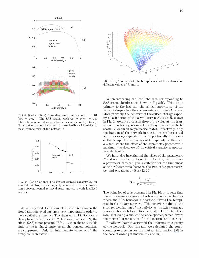
FIG. 10: (Color online) The bumpiness B of the network fordifferent values of R and a.

When increasing the load, the area corresponding toSAS states shrinks as is shown in Fig.8(b). This is dueprimary to the fact that the critical capacity αc of thenetwork drops when the system enters into the SAS state.More precisely, the behavior of the critical storage capac-ity as a function of the asymmetry parameter R, shownin Fig.9, presents a drastic drop of its value at the tran-sition from homogeneous retrieval (symmetric) state tospatially localized (asymmetric state). Effectively, onlythe fraction of the network in the bump can be excitedand the storage capacity drops proportionally to the sizeof the bump. For the values of the sparsity of the codea = 0.4, where the effect of the asymmetry parameter ismaximal, the decrease of the critical capacity is approx-imately twofold.

We have also investigated the effect of the parametersR and a on the bump formation. For this, we introducea parameter that can give a criterion for the bumpinessas the relative ratio between the two order parametersm0 and m1, given by Eqs.(22-26):

B =

√

m12

m02 + m1

2.

The behavior of B is presented in Fig.10. It is seen thatthe simultaneous increase of both R and a inside the areawhere the SAS behavior is observed, favors the bumpi-ness in the binary network. This behavior is due to thestronger localization of the activity as the extra term Ha

favors states with lower total activity. From the otherside, increasing a makes the code sparser, which favorsthe metrical organization of both patterns and neurons.

Finally we have investigated the information capacityof the network. For this aim we calculated the corre-sponding expression for the mutual information [20] inthe case of order parameters m0 and m1:

11

0 0.2 0.4 0.6 0.8Asymmetry retrieval factor R

0

0.05

0.1

0.15

Info

rmta

ion

Cap

acity

I [b

it]

0.00.20.4

0.4 0.5 0.6 0.70

0.005

0.01

Sparsity a(a)

0 0.2 0.4 0.6 0.8Asymmetry Retrieval Factor R

0

0.2

0.4

0.6

0.8

1

m0 �

��,m

1

m0

m1

(b)

FIG. 11: (Color online) (a) The information capacity versusthe asymmetry retrieval factor R for different values of thesparsity a. (b) m0, m1 for a = 0.2. The inside figure in (a)shows the behavior of the information capacity near the pointwhere it sharply decreases to zero.

IM (m0, m1, α) =α(m0 + 1)

2ln(m0 + 1)

+α|m1|

πF

[{

1

2, 1, 1

}

,

{

3

2,3

2

}

,m1

2

(1 + m0)2

]

+α(m0 + 1)

2ln

[

1

2+

1

2

√

1 − m12

(1 + m0)2

]

. (36)

Here F [.] is the hyper geometric function [21]. The firstterm is the normal expression for the mutual informa-tion (the sparsity of the code eliminates the symmetrybetween m and −m). The next two lines of the equationcan be regarded as a correction to the usual expressiondue to OP m1 6= 0.

With the aim of Eqs.(22-26) and the above expres-sion, for the information capacity IM/cN we obtainedthe behavior, presented in Fig.11, which has been alsoreproduced by simulations. This behavior is non trivialand shows a well pronounced maximum for intermediatevalues of the sparsity of the code a. The correspondingbehavior of the order parameters m0 and m1, presentedin Fig.11(b), shows that inside the SAS region, their val-ues are significantly different form zero, but the informa-

tion capacity is very small although non zero. If fromone side, the information capacity IM/cN , measures thenumber of bits, needed to represent the state and if fromthe other side, the overlap parameters (m0, m1) measurethe degree to which one learned state can be recovered,then having small information capacity and large OPm0, m1 means that the original state can be recoveredwell with very small amount of information. This resultcould be useful for effective retrieval of patterns by usingvery small amount of information, especially in combi-nation with the observed improvement of the stability ofthe network, provided that the retrieval starts from thebump.

Similar results have been reported in [2] with respectto the increase of the computational power of the struc-tured network. The last is expressed by the ability ofthe network to retrieve several patterns, each in a dif-ferent location, whose combination could form the globalcombinatorially large pattern.

Apart of the advantage of the localized states in termsof the minimal cost in transferring information, suchstructures could have important biological relevance forthe cortical modules of the mammalian brain, which arecharacterized by geometrical distribution of the synap-tic connections. Recent experiments of the activity ofa macaque temporal cortex [22] have demonstrated thatthe receptive fields of the visual evoked activity patternsare restricted up to three fold, when several patterns arepresent together. The last result seems to be coherentwith the picture of localized activity in a neural networkwith metric organization of the synaptic activities.

V. CONCLUSION

In this paper we have studied the spatially dependentactivity in a binary neural network model when retrievaland learning states have certain degree of asymmetry. Wehave shown that nor asymmetry of the connections, nei-ther sparsity of the code are necessary to achieve bumpsolutions for the activity of the network, but rather dif-ferent symmetry between the retrieval and the learningstates.

The extension of the classical method of Amit et al.[15] in the case of spatially dependent connectivity haspermitted, within some approximations, the derivation ofthe above results analytically. The good correspondencewith simulations, tested for different topologies of thenetwork, is also discussed through the paper.

We have shown that the region of the spatially asym-metric states is relatively large in the parameter space(R, a) and we have measured quantitatively how thebumpiness of the network depends on these two param-eters.

A drop of the critical storage capacity is observed in thetransition form symmetric to SAS states, which is due tothe fact that effectively only the fraction of the network inthe bump can be excited and the storage capacity drops

12

proportionally to the size of the bump.When the recovering of the pattern starts from a state

corresponding to the bump formation, the network be-haves in a better way in terms of stability and capacity,compared to the case of uniform initial conditions. Thishappens even if the overlap with the uniform initial con-ditions is significantly larger. The latter result could ar-gue the biological relevance of the bump formations foreffective retrieval of information.

Finally we have discussed the behavior of the infor-mation capacity versus the asymmetry retrieval factor Rand we have discussed its sharp decrease in the paramet-ric region, where bump formations are present.

Acknowledgments

The authors thank A.Treves and Y.Roudi for stimu-lating discussions at the early stage of work as well asthe Abdus Salam Center for Theoretical Physics for thefinancial support at the beginning of the present inves-tigation. E.K. and K.K. also acknowledge the financialsupport from the Spanish Grants DGI.M.CyT.FIS2005-1729 and TIN 2004–07676-G01-01 respectively.

[1] Y.Roudi and A.Treves, JSTAT, P07010, 1 (2004).[2] Y.Roudi and A,Treves, cond-mat/0505349.[3] K.Koroutchev and E.Korutcheva, Preprint ICTP, Tri-

este, Italy, IC/2004/91, 1 (2004).[4] K.Koroutchev and E.Korutcheva, Central Europ.

J.Phys., 3, 409 (2005).[5] A.Anishchenko, E.Bienenstock and A.Treves,

q-bio.NC/0502003.[6] J.Rubin and A.Bose, Network: Comput.Neural Syst., 15,

133 (2004).[7] N.Brunel, Cereb.Cortex, 13, 1151 (2003).[8] V.Breitenberg and A.Schuz, Anatomy of the Cortex,

(Springer, Berlin,1991).[9] D.J.Watts and S.H.Strogatz, Nature, 393, 440 (1998).

[10] D.J.Watts, Small Worlds: The Dynamics of NetworksBetween Order and Randomness(Princeton Review inComplexity) (Princeton University Press, Princeton, NewJersey, 1999).

[11] M.Tsodyks and M.Feigel’man, Europhys.Lett., 6, 101(1988).

[12] D.Bolle, G.Shim, B.Vinck and V.A.Zagrebnov, Journal

of Stat.Phys., 14, 565 (1994).[13] J.Hopfield, Proc.Natl.Acad.Sci.USA, 79, 2554 (1982).[14] D.Hebb, The Organization of Behavior: A Neurophysio-

logical Theory, (Wiley, New York, 1949).[15] D.Amit, H.Gutfreund and H.Sompolinsky, Ann.Phys.,

173, 30 (1987).[16] N.N.Bogolyubov, Physica(Suppl.), 26, S1 (1960).[17] M.Mezard, G.Parisi and M.-A.Virasoro, Spin-glass the-

ory and beyond, (World Scientific, Singapore, 1987).[18] A.Canning and E.Gardner, Phys.A:Math.Gen., 21, 3275

(1988).[19] I.Farkas et al., Phys. Rev.E 64, 026704 (2001).[20] R.Blahut, Principle and Practice of Information Theory,

(Addison-Wesley, Cambridge MA, 1988).[21] M.Abramowitz and I.A.Stegun, Handbook of Mathemati-

cal Functions With Formulas, Graphs, and MathematicalTables, (National Bureau of Standards, Applied Mathe-matics Series-55, 1972).

[22] E.Rolls, N.Aggelopoulos and F.Zheng, J.Neurosci. 23,339 (2003).