arX

iv:c

ond-

mat

/980

7101

v1 [

cond

-mat

.dis

-nn]

7 J

ul 1

998

Attractor neural networks storing multiple space representations: a model for

hippocampal place fields

F. P. Battaglia and A. TrevesNeuroscience, SISSA, Via Beirut 2-4, 34014 Trieste – Italy

A recurrent neural network model storing multiple spatial maps, or “charts”, is analyzed. Anetwork of this type has been suggested as a model for the origin of place cells in the hippocampusof rodents. The extremely diluted and fully connected limits are studied, and the storage capacityand the information capacity are found. The important parameters determining the performance ofthe network are the sparsity of the spatial representations and the degree of connectivity, as foundalready for the storage of individual memory patterns in the general theory of auto-associativenetworks.

Such results suggest a quantitative parallel between theories of hippocampal function in differentanimal species, such as primates (episodic memory) and rodents (memory for space).

I. INTRODUCTION

Knowledge of space is one of the main objects of com-putation by the brain. It includes the organization ofinformation of many kinds and many origins (memory,the different sensory channels, and so on) into mentalconstructs, i.e. maps, which retain a geometrical natureand correspond to our perception of the outer world.

Every animal species appears to have specialized sys-tems for spatial knowledge in some region of the brain,more or less well developed and capable of performingsophisticated computations. For rodents there is a largeamount of experimental evidence that the hippocampus,a brain region functionally situated at the end of all thesensory streams, is involved in spatial processing. Manyhippocampal cells exhibit place related firing, that is,they fire when the animal is in a given restricted region ofthe environment (the “place field”), so that they containa representation of the position of the animal in space.

The hippocampus, one of the most widely studiedbrain structures, shares the same gross anatomical fea-tures across mammalian species, nevertheless it is knownto have different functional correlates for example in pri-mates and humans (where it is believed to be involvedin episodic memory, roughly, memory of events) and inrodents, in which it is mainly associated to spatial rep-resentation.

One relevant feature of the hippocampus which ismaintained across species is a region, named CA3, char-acterized by massive intrinsic recurrent connections. Itwas appealing for many theorists to model this regionas an auto-associative memory storing information in itsintrinsic synaptic structure, information which can be re-trieved from small cues by means of an attractor dynam-ics, and which is represented in the form of activity con-figurations.

Within the episodic memory framework, each attrac-tor configuration of activity is the internal representationof some memory item. The CA3 auto-associative net-

work can be seen as the heart of the hippocampal system,containing the very complex, inter-modal representationspeculiar to episodic memory. Auto-associative, or attrac-tor neural networks have been extensively studied withthe tools of statistical physics [1]. Efficiency measures,like the number of storable memory items or the qualityof retrieval, can be computed for any appropriately de-fined formal model. An intensive effort was performedto embed in this idealized models more and more ele-ments of biological realism, trying to capture the relevantanatomical and functional features affecting the perfor-mance of the network. It was then found that a theory ofthe hippocampus (or, more precisely, CA3) as an auto-associative network has as its fundamental parametersthe degree of intrinsic connectivity, i.e. the average num-ber of units which send connections to a given unit, andthe sparsity of the representations, roughly the fractionof units which are active in one representation. These pa-rameters have biological correlates that are measurablewith anatomical and neurophysiological techniques.

Spatial processing, as it is performed by the rodenthippocampus, also involves memory of some kind; recentexperimental evidence support the idea that spatially re-lated firing is not driven exclusively by sensory inputs butalso reflects some internal representation of the exploredenvironment. First, place fields are present and stablealso in the dark, and in condition of deprived sensory ex-perience. Second, completely different arrangements ofplace fields are found in different environments or evenin the same environment in different behavioral condi-tions.

These findings have led to hypothesize that CA3 (like,perhaps, other brain regions with dense connectivity)stores “charts”, representations of environments in theform of abstract manifolds, on which each neuron cor-responds to a point, that is the center of its place field.Place fields arise as a result of an attractor dynamics,whose stable states are “activity peaks” centered, in thechart space, at the animal’s position. It is important to

1

note that the localization of each neuron on a chart doesnot appear to be related to its physical location in theneural tissue.

The positions of place fields are encoded by the recur-rent connections, and it is possible to store many differ-ent charts in the same synaptic structure, just as manydifferent patterns are stored in a Hopfield net, for ex-ample, and different activity peaks can be successivelyevoked by appropriate inputs, just as it happens withauto-associative memories.

It is interesting to address the issue of whether anepisodic memory network and the “spatial multi-chart”memory network share the same functional contraints,so that a biological brain module capable of performingone of the tasks is also adequate for the other. Herewe present a statistical mechanics analysis of the multi-chart network, focusing on the parallel with autoassocia-tive memory in the usual (episodic memory) sense. It isfound that the performances of these two networks aregoverned by very similar laws, if the parallel betweenthem is drawn in the appropriate way.

In sec. II the case of a single attractor chart stored isstudied, then in sec. III the case of multiple stored chartsis analyzed and the storage capacity is found, first fora simplified model and then for a more complex modelwhich makes it possible to address the issue of sparsityof representations. In sec. IV the storable information ina multi-chart network is calculated, making more precisethe sense in which such a network is a store of informa-tion, and completing the parallel with auto-associativememories.

II. THE SINGLE MAP NETWORK

As a first step, we consider the case of a single at-tractor map encoded in the synaptic structure, as it wasproposed in [2]. We focus here on the shape and prop-erties of the attractor states, as a useful comparison forthe following treatment of the multiple charts case.

The neurons are modelled as threshold linear units,with firing rate:

Vi = g[hi − θ]+ = g(hi − θ)Θ(hi − θ) (1)

i.e. equal to zero if the content of the square brackets isnegative. h represents the synaptic input current, com-ing from other cells in the same module, θ is a firingthreshold, which may incorporate the effect of a subtrac-tive inhibitory input, common to all the cells, as it willbe illustrated later on. The connectivity within the mod-ule is shaped by the selectivity of the units. If ri is theposition of the center of the place field of the i-th cell,in a manifold M , of size |M |, corresponding to the en-vironment, the connection between cells i and j may be

expressed as

Jij =|M |N

K(|ri − rj |), (2)

where K is a monotone decreasing function of its argu-ment.

The synaptic input to the i-th cell is therefore givenby

hi =∑

j

JijVj =∑

j

|M |N

K(|ri − rj |)Vj . (3)

If the number N of cells is large, and the place fieldscenters (p.f.c.) are homogeneously distributed over theenvironment M (be it one or two-dimensional), we canreplace the sum over the index j with an integration overthe coordinates of the p.f.c:

h(r) =

∫

M

dr′K(|r− r′|)V (r′). (4)

Note that the normalization in eq. 2 is chosen in orderto keep the synaptic input to a given unit fixed when |M |varies and the number of units is kept fixed, that is, thedensity of p.f.c.s N/|M | varies (the |M | factor will thencompensate for the fewer input units within the range ofsubstantial K strength). A fixed-point activity configu-ration must have the form

V (r) = g

[∫

M

dr′K(|r − r′|)V (r)′ − θ

]+

. (5)

We could write eq. 5 as

V (r) =

g(∫

Ω dr′K(|r − r′|)V (r′) − θ) r ∈ Ω0 r 6∈ Ω

(6)

where Ω is a domain for which there exists a solution ofeq. II that is zero on the boundary.

If only solutions for which Ω is a convex domain areconsidered, the fact that V (r) is zero on ∂Ω will ensurethat units with p.f.c. outside Ω are under threshold,therefore their activity is zero and solutions of eq. II areguaranteed to be solutions of eq. 5. The size and theshape of the domain Ω in which activity is different fromzero is determined by eq. II. As a first remark, we noticethat it is independent from the value of the threshold θ.In fact, if Vθ is a solution of (II) with threshold θ, giventhe linearity of eq.II within Ω,

Vθ′ =θ′

θVθ

will be a solution of the same equation with θ′ instead ofθ, with the same null boundary conditions on Ω. Rescal-ing the threshold will then have the effect of rescal-ing the activity configuration by the same coefficient.This means that subtractive inhibition cannot shape, e.g.

2

shrink or enlarge, this stable configuration, and thereforeit is not relevant for a good part of the subsequent anal-ysis. Some form of inhibition is nevertheless necessary toprevent the activity from exploding. Moreover, there arefluctuation modes which cannot be controlled by overallinhibition as they leave the total average activity con-stant. They will be treated in sec. III C. It is found that,at least in the one dimensional case, these modes do notaffect stability in the single chart case.

In absence of an external input, any solution can be atmost marginally stable, because a translation of the solu-tion is again a solution of eq. II. An external, “symmetrybreaking” input, taken as small when compared to thecontribution of recurrent synapses, is therefore implicitin the following analysis.

A. The one-dimensional case

The case of a recurrent network whose attractors re-flect the geometry of a one-dimensional manifold, be-sides being a conceptual first step in approaching the2-dimensional case, is relevant by itself, for example inmodeling other brain systems showing direction selectiv-ity, e.g. in head direction cells [3,4], and also for placefields on one-dimensional environments [5].

In this case eq. II reads:

V (r) = g

(

∫ R

−R

K(|r − r′|)V (r′) − θ

)

V (R) = V (−R) = 0. (7)

For several specific forms of the kernel K it is possibleto solve explicitly eq. 7, yielding interesting conclusions.For example if:

K(|r − r′|) = e−|r−r′|, (8)

(see also [2]) differentiating eq. 7 twice yields:

V ′′(r) = −γ2V (r) + gθ, (9)

where γ =√

2g − 1.Solutions vanishing at −R and R (and not vanishing

in ] − R, R[), have the form:

V (r) = A cos(γr) +gθ

2g − 1, (10)

with

A = − gθ

(2g − 1) cos(γR). (11)

The value of R for which (10) is a solution of eq. 7 isdetermined by the integral equation itself: for example,by evaluating V ′(R) or V ′(−R) from eq. 7 we get:

V ′(−R) = −V ′(R) = gθ. (12)

Substituting (10) and (11) in eq. 12 we have:

tan(γR) = −γ

so that

R =tan−1(−γ) + nπ

γ.

Requiring R to be positive and V (x) to be positive for−R < r < R, leads to choose

R =− tan−1(γ) + π

γ, (13)

note that A > 0.R is then a monotone decreasing function of γ, and

therefore of the gain g.This is also true for other forms of the connection ker-

nel K. As an example, consider the kernel:

K(r − r′) = cos(r − r′) (14)

by a similar treatment it is shown that a solution is ob-tained with

R =1

g. (15)

The kernel

K(r − r′) = Θ(1 − |r − r′|)(1 − |r − r′|) (16)

will result in a peak of activity of semi-width

R =π√2g

. (17)

Equations of the type (5) have more solutions in addi-tion to the ones considered above, representing a singleactivity peak. For example, if we consider an infiniteenvironment, periodic solutions will be present as well,representing a row of activity peaks separated by regionsof zero activity. These solution can be checked to be un-stable if we model inhibition as an homogeneous termacting on all cells in the same way and depending on theaverage activity. Intuitively, if we perturb the solution byinfinitesimally displacing one of the peaks, it will tend tocollapse with the neighbor which has come closer.

3

B. The two-dimensional case

To model the place cells network in the hippocampuswe need to extend this result to a two dimensional envi-ronment. The equation for the neural activity will be:

V (r) = g

[∫

M

dr′K(|r − r′|)V (r′) − θ

]+

. (18)

The generalization to 2-D is straightforward if for thekernel K(|r−r′|) we consider the one with Fourier trans-form is

K(p) =2

1 + p2, (19)

(the two-dimensional analog of the kernel of eq. 8) thatis, a kernel resembling the propagator of a Klein-Gordonfield in Euclidean space. The fact that this kernel is di-vergent for (r − r′) → 0 does not give rise to particularproblems, since, in the continuum limit of eq. 4, the con-tribution to the field h coming from the nearby pointswill stay finite, and in fact two units will be assignedp.f.c’s so close to each other to yield a overwhelminglyhigh connection only with a small probability. Let uslook for a solution with circular symmetry such that ac-tivity V (r) is zero outside the circle of radius R, C(R). Ifwe apply the Laplacian operator on both sides of

V (r) = g

∫

C(R)

dr′K(r − r′)V (r′) − θ (20)

we obtain:

∇2V (r′) = −γ2V (r′) + gθ (21)

(again, γ2 = 2g − 1), which in polar coordinates reads:

V ′′(r) +1

rV ′(r) = −γ2V (r) + gθ. (22)

The solution is

V (r) = AJ0(γr) +gθ

2g − 1. (23)

J0 is the Bessel function of order 0. For the solutionto vanish on the boundary of C(R) one must take:

A =gθ

(2g − 1)J0(γR).

The other condition that determines R may be foundby substituting (23) in eq. 20. Here again, R(g) is amonotone decreasing function.

As in the one-dimensional case, solutions with a non-connected (or even non-convex) support can be seen notto be stable.

III. STORING MORE THAN ONE MAP

Let us imagine now that the p.f.c’s for each cell aredrawn with uniform distribution on the environmentmanifold M , and connections are formed according to(2). Several “space representations” may be created bydrawing again at random the r.p.c. of each cell from thesame distribution. The connection between each pair ofcells will then be the sum of a number of terms of theform (2), one for every “space representation”, or “map”,or “chart”. With p = αN maps, and the r.p.c. of the

i-th cell in the µ-th map indicated by x(µ)i :

Jij =

p∑

µ=1

|M |N

K(|r(µ)i − r

(µ)j |). (24)

The question that immediately arises is: what is thecapacity of this network, that is, how many maps can westore, so that stable activity configurations, correspond-ing to some region in the environment described by onemap, like the ones described by the solutions of eq. II,are present? The problem resembles the classic attractorneural network problem [1], with threshold linear units.A standard treatment has been developed [6] allowingto calculate the capacity of a network of threshold lin-ear units with patterns drawn from a given distributionand stored by means of a hebbian rule. The treatment isvery simplified in the extreme dilution limit [7,8]. In thenext sections it will be shown how this treatment can beextended to the map case, first for one particular formof the kernel K, leading to the solution of the capacityproblem for a fully connected network; in the following,the solution is extended to more general kernels, first inthe diluted limit, then for the fully connected network.

Another related question is: how much information isthe synaptic recurrent structure encoding, and in whichsense is the synaptic structure a store of information?The aim is to develop a full parallel between the multi-chart network and autoassociative networks, and if pos-sible to characterize the parameters constraining the per-formance of this system.

A. The fully connected network: “dot product”

kernel

Let us consider a manifold M with periodic boundaryconditions, that is, a circle in one dimension and a torusin two dimensions. The p.f.c. of a cell ri can then bedescribed by a 2-dimensional unit vector ~ηi for the one-dimensional case and by a pair of unit vectors ~η1,2

i forthe two dimensional case. Suppose now that the contri-bution from the µ-th map to the connection between celli and cell j is given by:

K(|r(µ)i − r

(µ)j |) =

d∑

l=1

(~ηl(µ)i · ~ηl(µ)

j + 1), (25)

4

so that

Jij =1

N

p∑

µ=1

d∑

l=1

(~ηl(µ)i · ~ηl(µ)

j + 1), (26)

where d is the dimensionality.p = αN is the number of stored charts. Eq. 25 de-

scribes an excitatory, very wide spread form for the ker-nel (2) (the contribution to the connectivity is zero onlyif the r.p.c.s of the two cells are at the farthest pointsapart, i.e. at 180). This spread of connectivity wouldlead to configurations of activity that are large in ther.p.c. space, that translated in auto-associative memorylanguage would be very “unsparse”, i.e. very distributedrepresentations. It is therefore plausible that this willseverely limit the capacity of the net. In any case, theform of (25), factorizable in one term depending on ~ηi andone term depending on ~ηj , after incorporating the con-stant part in a function b0(x), makes it possible to per-form the free energy calculation through Gaussian trans-formations as in [6]. A similar model has been studied in[9] with McCulloch-Pitts neurons.

A Hamiltonian useful to describe the thermodynamicsof such a system is

H = −1

2

∑

i,j( 6=i)

JijViVj − NB

(

∑

i

Vi

N

)

−

∑

l

∑

i

∑

µ

sl(µ) · ~ηl(µ)i Vi (27)

where B(x) =∫ x

b(y)dy, and b(x) is a function describ-ing an uniform inhibition term depending on the averageactivity in the net. sl(µ) is a symmetry breaking field,pointing in a direction in the µ−th map space. The meanfield free-energy in the replica symmetric approximationcan be calculated (the partition function is calculated asthe trace over a measure that implements the threshold-linear transfer function, see [6]). The presence of a phasewith spatially specific activity correlated with one mapwill be signaled by solutions of the mean field equationswith a non-zero value for the order parameter

xl(µ) =1

Nd

N∑

i=1

~ηl(µ)i Vi (28)

which plays the role of the overlap in an auto-associativememory. This parameter has the meaning of a popula-tion vector [10], that is, the animal position is indicatedby an average over p.f.c.s of the cells weighted by cellsactivity.

The set of resulting mean field equations can be re-duced to a set of two equations, eqs. A8 and A9, in twovariables, the “non-specific” signal-to-noise ratio, w, andthe “specific”, space related signal-to-noise ratio v. Thedetails of the calculation are reported in Appendix A.

The critical value αc indicating the storage capacityof the network is the maximum value for which eq. A8

still admits solutions corresponding to space related ac-tivity (non-zero v) and may be found numerically. Atthis value αc the system undergoes a first-order phase-transition towards a state in which no space-related ac-tivity is possible. Eq. A9 gives the range of gain valuesfor which there exist solutions at a given α ≤ αc [6].

In this model there is no possibility for modulatingthe spread of connections in the chart-space. As we an-ticipated, the activity configurations that one obtains arevery wide, with a large fraction of units active at the sametime. Cells will have very large place fields, covering alarge part of the environment (of the order of roughlyone half for the one dimensional case, and roughly onequarter for the two-dimensional case). As one would in-fer from the analysis of autoassociative memories storingpatterns, for example binary, these “unsparse” represen-tations of space will lead to a very small capacity of thenet.

For the model defined on the one-dimensional circlethe capacity found is αc ∼ 0.03. At this value the systemundergoes a first order transition. As α increases beyondαc, x jumps discontinuously from a finite value to zero.

The capacity for the diluted analogue of this model(see [8], Appendix A and section III B) is given by theequation

E1(w,v) ≡ [(1 + δ)A2]2 − αA3 = 0. (29)

Remember that in this case p = αcN where c is the con-nectivity fraction parameter, see section III B. In thiscase αc ∼ 0.25. At αc the transition is second order,with the “spatial overlap” x approaching continuouslyzero, verified at least with the precision at which it waspossible to to solve numerically eq. 29. For the 2-D case,storage capacities are αc ∼ 0.0008 for the fully connectednetwork and α ∼ 0.44 for the diluted network.

To get a larger capacity, and to provide a possible com-parison with the experimental data from the hippocam-pus, in which the tuning of place fields is generally nar-row, we must extend our treatment to more general ker-nels, and this will be done in the following two sections.

B. Generic kernel: extremely diluted limit

Consider a network in which every threshold-linearunit, whose activity is denoted by Vj , senses a field:

hi =1

c

∑

j 6=i

CijJijVj , (30)

where Jij is given by eq. 24. From now on the kernel Kis defined as

K(~r − ~r′) = K(~r − ~r′) − K

K =⟨⟨

K(~r − ~r′)⟩⟩

(31)

5

for any ~r, where 〈〈. . . 〉〉 means averaging over ~r. With

this notation, whatever the original kernel K, K is thesubtracted kernel which averages to zero. The manifoldM is taken with periodic boundary condition (that is acircle in one dimension and a torus in the two dimensionalcase).

Cij is a “dilution matrix”

Cij =

1 with prob. c,0 with prob. 1 − c

(32)

and Nc/ logN → 0 as N → ∞. In the thermodynamiclimit N → ∞ the activity of any two neurons Vi and Vj

will be uncorrelated [7]. A number of charts p = αcNis stored. Looking for solutions with one “condensed”map, that is, solutions in which activity is confined tounits having p.f.c. for a given chart in a certain neigh-borhood, it is possible to write the field hi as the sumof two contributions, a “signal”, due to the condensedmap and a “noise” term, ρz – z being a random variablewith Gaussian distribution and variance one – due to allthe other, uncondensed, maps, namely, in the continuumlimit, labeling units with the position ~r1 of their p.f.c. inthe condensed map,

h(~r1) = g

∫

M

d~r1′

K(~r1 − ~r1′

)V (~r1′

) + ρz; (33)

the noise will have a variance

ρ2 = αy|M |2〈〈K2(~r − ~r′)〉〉, (34)

where

y =1

N

N∑

i=1

〈V 2i 〉. (35)

The fixed point equation for the average activity profilex1(~r) is

x1(~r) = g

∫ +

Dz(h(~r) − θ). (36)

where again Dz is the Gaussian measure, and

h(~r) =

∫

d~r′K(~r − ~r′)x1(~r′) + b(x) − ρz (37)

and

x =

∫

d~r

|M | x1(~r) (38)

is the average overall activity. The average squared ac-tivity (entering the noise term) will read:

y = g2

∫

d~r

|M |

∫ +

Dz(h(~r) − θ)2. (39)

The fixed point equations may be solved introducingthe rescaled variables

w =b(x) − θ

ρ(40)

v(~r) =x1(~r)

ρ. (41)

The fixed point equation for v(~r) is

v(~r) = gN(∫

d~r′K(~r − ~r′)v(~r′) + w

)

(42)

where

N (x) = xΦ(x) + σ(x), (43)

(Φ(x) and σ(x) are defined in eq. A16 and eq. A17) isa “smeared threshold linear function”, monotonically in-creasing, with

limx→−∞

N (x) = 0

and

limx→+∞

N (x)/x = 1.

In terms of w and v(~r), y reads:

y = ρ2g2

∫

d~r

|M |M(∫

d~r′K(~r − ~r′)v(~r′) + w

)

(44)

where

M(x) = (1 + x2)Φ(x) + xσ(x). (45)

By substituting eq. 44 in eq. 34, we obtain

1

α= g2|M |〈〈K〉〉

∫

d~rM(∫

d~r′K(~r − ~r′)v(~r′) + w

)

.

(46)

If we can solve eq. 42 and find v(~r) as a function of wand g, a solution is found corresponding to a value of αgiven by eq. 46. To find the critical value of α, we haveto maximize α over w and g.

The mathematical solution of eq. 42 is treated in Ap-pendix B.

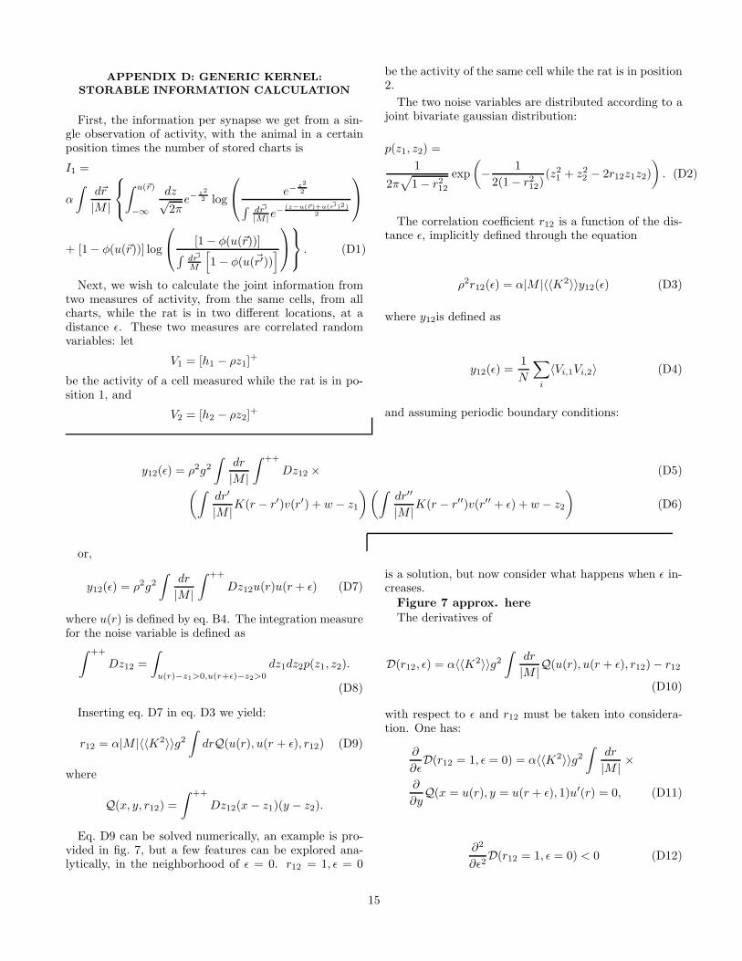
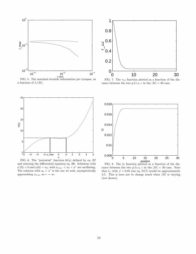
With this model, we can modulate the spread of con-nections by acting on K(~r−~r′) or alternatively, by vary-ing the size of the environment. The results are depictedin fig. 1 for the 1-D circular environment and in fig. 2 forthe 2-D toroidal environment (upper curves). Examplesof the solutions of eq. 42 are displayed in fig. 3 for the1-D environment and in fig. 4 for the 2-D environment.

We note that, as the environment gets larger in com-parison to the spread of connections (therefore, to thesize of the activity peak), the capacity decreases approx-imately as

αc ∼ −1/ log(am) (47)

6

where am is the map sparsity and it is equal to:

am =kd

|M | (48)

where kd is a factor roughly equal to ∼ 4.5 for the 1-Dmodel and ∼ 3.6 for the 2-D model.

That is, the sparser the coding, the less the capacity.This is, at first glance, in contrast with what is knownfrom the theory of auto-associative networks, in whichsparser representations usually lead to larger storage ca-pacities.

For comparison, keeping the formalism of [6], forthreshold-linear networks with hebbian learning rule, en-coding memory patterns rii=1...N with sparsity a de-fined as

ap =〈〈r〉〉2〈〈r2〉〉

(for binary patterns this is equal to the fraction of activeunits), and for small a, the capacity is given by

αp ∼ 1

ap log(1/ap). (49)

The apparent paradox (larger capacity with sparserpatterns, smaller with sparser charts) is solved as onerecognizes that each chart can be seen as a collectionof configurations of activity relative to different points

in space covering, as in a tiling, the whole environment.Each configuration is roughly equivalent to a pattern inthe usual sense. Intuitively, and in sense that will madeclearer below, a chart is equivalent, in terms of “use ofsynaptic resources” to a number proportional to a−1

m ofpatterns of sparsity am.

The proportionality coefficient, or equivalently, the dis-tance at which different configurations are to be consid-ered to establish a correct analogy, will be dealt with inAppendix D.

These considerations and the comparison of eq. 47 andeq. 49 make clear that αc is the exact analogue of thepattern autoassociators’ αp.

Figures 1, 2, 3, 4, approx. here

C. Inhibition independent stability

The dynamical stability of the solutions of eq. 42 is ingeneral determined by the precise functional form chosenfor the inhibition, which we assumed a function of theaverage overall activity in the net. Nevertheless, thereare fluctuations modes which leave the average activityunaltered. Stability against these modes is therefore un-affected by the inhibition and may be checked alreadyfor a general model. Let us consider a “synchronous”dynamics, that is, all the neurons are updated simulta-neously at each time step. The evolution operator for thevariables V (r, t) and ρ(t) is:

V (r, t + 1) = gρ(t)N(∫

M

dr′

|M |K(r − r′)V (r′, t)

ρ(t)+

b(x(t))

ρ(t)

)

(50)

ρ2(t + 1) = g2α|M |ρ2(t)〈〈K2〉〉∫

M

drM(∫

M

dr′

|M |K(r − r′)V (r′, t)

ρ(t)+

b(x(t))

ρ(t)

)

. (51)

This evolution operator has as its fixed points V0(r) = ρ0v0(r) and ρ0 where v0(r) and ρ0 are the solutions of eq. 42,34, and 44, i.e. the stable states of our system.

We can linearize the evolution operator around (V0(r), ρ0) and look for fluctuation modes (eigenvectors) (δV (r), δρ)with

∫

M

dr δV (r) = 0 (52)

We obtain the following equations:

λδV (r) = gΦ(u0(r))

[∫

M

dr′K(r − r′)δV (r′)

]

+ gσ(u0(r))δρ (53)

λδρ =

(

1 − 1

2gα|M |〈〈K2〉〉

∫

M

dru0(r)v0(r)

)

δρ +1

2gα|M |〈〈K2〉〉

∫

M

dru0(r)δV (r), (54)

where

u0(r) = N−1

(

v0(r)

g

)

.

7

Inserting eq. 53 in eq. 52:

δρ = −∫

Mdr′Φ(u0(r))

[∫

MdrK(r − r′)δV (r′)

]

∫

M drσ(u0(r))(55)

Eq. 55 can be inserted again in eq. 53, obtaining aclosed integral equation in δV . Unfortunately, this equa-tion is very difficult to solve, but we can derive a stabilitycondition by making an ansatz on the form of the eigen-function δV (r). More precisely, let us concentrate onthe 1-D case. We look for solutions with even symme-try (we know there must be an eigenfunction with oddsymmetry, and eigenvalue equal to 1, corresponding to acoherent displacement of the activity peak). This kindof solution corresponds to spreading and shrinking of theactivity peak. Let us assume that the even eigenfunctionwith the highest eigenvalue (the most unstable) has onlytwo nodes (an even eigenfunction must have at least twonodes because of eq. 52), at r0 and −r0. Let us takethe sign of the eigenfunction δV (r) such that δV (0) > 0.From eqs. 52 and 55 we see that

δρ < 0.

Now, from eq. 54:

λ =

(

1 − 1

2gα|M |〈〈K2〉〉

∫

M

dru0(r)v0(r)

)

+

1

2gα|M |〈〈K2〉〉

∫

M

dru0(r)δV (r)

δρ, (56)

and we recognize that

∫

M

dru0(r)δV (r)

δρ< 0.

Thus,

λ < 1 − Γ

2(57)

with

Γ = gα|M |〈〈K2〉〉∫

M

dru0(r)v0(r). (58)

Thus, if the ansatz we formulated holds, we have astability condition Γ > 0, which is found to be fulfilledfor all the solutions we found relative to maximal storagecapacity. This implies that the storage capacity resultis not affected by instability of the solutions, providedof course that an appropriate form for inhibition is cho-sen. This stability result is also related to the correlationin the static noise for two solutions centered at differentp.f.c.s, as we will show in App. D.

It can also be shown that by taking the α → 0 limit(i.e. the single chart case), one always has Γ > 0 since itis v0(r) = 0 when u0(r) < 0.

D. The fully connected model

The treatment of the model with the fully connectednetwork and a kernel K for connection weights satisfyingthe condition (31) will use the replica trick to averageover the disorder (the realizations of the ~r’s) and willeventually lead to a non-linear integral equation for theaverage activity profile in the space of the “condensedmap” very similar to eq. 42. Let the Hamiltonian of thesystem be

H = −1

2

∑

i,j( 6=i)

JcijViVj − NB

(

∑

i

Vi

N

)

−

∑

i

∑

µ

sl(µ) · r(µ)i Vi (59)

where now the Jcij are given by (24) with a generic kernel

K(~r − ~r′) = K(~r − ~r′) − K (60)

where, again,

K = 〈〈K(~r − ~r′〉〉.

The free energy calculation is sketched in Appendix C.Again, the stable states of the system are governed bymean field equations. The mean field equation, eq. C16is an integral equation in the functional order parameterv(~r), the average space profile of activity.

If we are able to solve eq.C16 and find vσ(~r) as a func-tion of w and g′, by substituting eq. C17 and eq. C18in eq. C11 we have an equation that gives us the valueof α corresponding to that pair (g′, w). αc is then themaximum of α over the possible values of (g′, w).

To solve eq. C16, it is easy to verify that if v(~r) is asolution of

v(~r) = g′N(∫

M

d~r′K(~r − ~r′)v(~r′) + w

)

(61)

with

w = w − K

∫

M

d~r v(~r)

that is, the same equations as eqs. B2 and B3, then

v(~r) =

∫

M

d~r′[

L(~r − ~r′) − L]

v(~r′)

8

is a solution of eq. C16. v can therefore be interpretedas the average activity profile, apart from a constant.Eq. 61 can be solved with the same procedure used foreq. 42, and the maximum value of α can be found bymaximizing over g′ and w.

The results for 1-D and 2-D environment are depictedin fig. 1 and 4 (lower curves). As we may expect frompattern autoassociator theory, the capacity is much lowerthan for the diluted model, due to an increased interfer-ence between different charts.. As the sparsity a ∼ 1/|M |gets smaller, the capacities of the two models get closer,both being proportional to 1

log(|M|) . Reducing the spar-

sity parameter of space representations has therefore theeffect of minimizing the difference between nets withsparse and full connectivity.

E. Sparser maps

A possible extension of this treatment is inspired fromthe experimental finding that, in general, not all the cellshave place cells in a given environment. Ref. [11] e.g. re-ported that ∼ 28−45% of pyramidal cells of CA1 have aplace field in a certain environment. We would like to seehow this fact could affect the performance of the multi-chart auto-associator. It is then natural to introduce anew sparsity parameter, the chart sparsity ac indicatingthe fraction of cells which participate in a chart. Wewill show that, for the capacity calculation, a−1

c “sparse”charts are equivalent to a single “full” chart, of size a−1

c .We will present the argument for the diluted case, thefully connected case is completely analogous.

Let mµi be equal to 1 if cell i participates in chart µ,

that is with probability ac. Thus, the synaptic couplingJij will read

Jij =

p∑

µ=1

|M |acN

K(x(µ)i − x

(µ)j )mµ

i mµj . (62)

Let us consider a solution with one condensed map:cells participating with p.f.c. in r in that map will havea space related signal-to-noise ratio

v(~r) = gN(∫

d~r′K(~r − ~r′)v(~r′) + w

)

(63)

for all the neurons not participating in the condensedmap we will have

v = N (w). (64)

The noise will have a variance

ρ2 = αacy

( |M |ac

)2

〈〈K2(~r − ~rµ〉〉, (65)

that is ac times the value we would get for the samenumber of “full” charts with size |M |/ac. and now

y = ρ2g2

ac

∫

M

d~r

|M |M(∫

d~r′K(~r − ~r′)v(~r′) + w

)

+

(1 − ac)M(w) . (66)

By comparing eq. 44 and eq. 66, and remembering thatfor ~r far from the activity peak, v(~r) ∼ N (w) we real-ize that this y value is approximately equivalent to the yvalue we would get for “full” charts of size |M |/ac.

Inserting eq. 65 and eq. 66 in eq. 46, one finds, for themaximal capacity:

αc (sparse charts) ∼1

ac log( |M|ac

). (67)

As we anticipated one may interpret this result as fol-lows: the capacity is the same as if we had taken a−1

c

“sparse” charts, including ∼ N cells, and put them sideby side to form one single “full” chart. If we have startedwith αC “sparse” charts we now have have acαC “fullcharts”. From eq. 46 we see that we can store at mostαc (full charts)C full charts and

αc (full charts) ∼1

log( |M|ac

)

and this explains eq. 67. Therefore, this network is as ef-

ficient in terms of spatial information storage as the oneoperating with full charts.

IV. INFORMATION STORAGE

Like a pattern auto-associator, the chart auto-associator is an information storing network. The cog-nitive role of such a module could be to provide a spatialcontext to information of non-spatial nature containedin other modules, which connect with the multi-chartmodule. Each chart represents a different spatial or-ganization, possibly related to a different environmen-tal/behavioral condition. Within each chart, a cell isbound to a particular position in space, thus being themeans for attaching some piece of knowledge to a par-ticular point in space, through inter-module connections.To give a very extreme, unrealistic, but perhaps useful,example, let us assume that each cell encodes a partic-ular discrete item, or the memory of some events hap-pened somewhere in the environment, as in a “grand-mother cell” fashion, encoding “the grandmother sittingin the armchair in the dining room”. The encoding ofthe “grandmother” may be accomplished by some set ofafferents from other modules. The multi-chart associatorcan then attach a spatial location to that memory of the“grandmother”. The spatial location encoded is ideallyrepresented for each cell by its p.f.c.

In this sense, the information encoded in the network,which can be extracted by measures of the activity of the

9

units, is the information about the spatial tuning of theunits, that is their p.f.c.s.

To restate this concept in a formal way, we look for

Is = limS→∞

1

CN

∑

µ

∑

i

I( ~rµi , V µ(k)

i k=1...S) (68)

that is the information per synapse that can be extractedfrom S different observations of activity of the cells withthe animal is in S different positions , and the systemin activity states related to chart µ. This quantity doesnot diverge as S → ∞, since repeated observations ofactivity with the animal in nearby positions do not yieldindependent information, because of correlations betweenactivity configurations, correlations which decrease withthe distance at which the configurations are sampled.

The full calculation of this quantity involves a func-tional integration over the distribution of noise affectingcell activity as the animal is moving, and exploring thewhole environment. In Appendix D we suggest a proce-dure to approximate this quantity based on an “informa-tion correlation length” lI such that samples correspond-ing to animal positions at a distance lI yield approxi-mately independent information.

Is is the amount of spatial information which is storedin the module. It is the exact analogue of the stored in-formation for pattern auto-associators [6]. As for storagecapacity, it is to be found numerically, by maximizationover w and g.

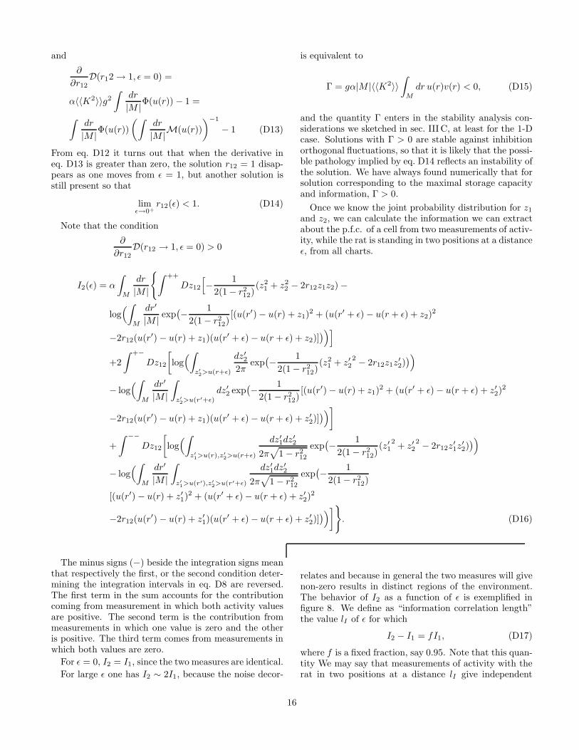
As for the capacity one can find the solution whichmaximizes Is. The resulting Imax is a function of the sizeof the relative spread of connections a = 1/|M |, and itamounts to a fraction of bit per synapse (see fig. 5).

figure 5 approx. here

As with pattern auto-associators, the informationstored increases with sparser representations. The in-crease is more marked for the fully connected network.For very sparse representations the performance of thefully connected model approaches the extreme dilutionlimit.

V. DISCUSSION

We have studied the multi-chart threshold linear as-sociator, as a spatial information encoding and storagemodule. We have given the solution for the dot-productkernel model, then we have introduced a formalism inwhich the generic kernel problem is soluble.

The second treatment has the advantage of providinga form for the average activity peak profile, which can becompared with the experimental data (see for example[9], fig.1).

We have shown that the non-linear integral mean fieldequation (eq. 42) can be solved at least for one class ofconnection kernels K(r − r′).

The storage capacity for both models has been found.We note that the capacity for the dot-product model iscompatible with the wide kernel (non sparse) limit of thegeneric model in one and two dimensions in the fully con-nected and in the diluted condition.

The generic kernel treatment makes it possible to ma-nipulate the most relevant parameter for storage effi-ciency, i.e. the spread of connections. It is shown thatthis parameter plays a very similar role as sparsity forpattern auto-associators. In the multi-chart case, more-over, the effective sparsity of the stable configurations isdetermined also by the value of the gain parameter g,as shown analytically for the noiseless case. Neverthe-less, the capacity of the network depends on the spreadof connection parameter ac = kd/|M | through a relationwhich is the exact analogue of the relation between spar-sity and capacity for the pattern auto-associator, at leastin the very sparse limit.

We have only considered here the capacity problem forone form of the connection kernel, although the treat-ment we propose is applicable, at least, to the other ker-nels considered for the noiseless case. Our hypothesis isthat a similar law for sparsity is to be found as eq. 47, atleast in the high sparsity limit, for more general forms ofthe kernel.

We have then shown that the capacity scales in sucha way that the information stored is not changed whenonly a fraction of the cells participate in each chart. Inthis case the firing of a cell carries information not onlyabout the position of its p.f.c. in the chart environment,but also about which environment the cell has a place-field in. This information adds up, so that 1/ac chartscan be assembled in a single larger chart of size 1/ac

times larger.We have introduced a definition of stored information

for the multi-chart memory network, which measures thenumber of effective different locations which can be dis-criminated by such a net: representations of places at adistance less than lI are confused, because of the finitewidth of the activity peaks, and because of the staticnoise.

lI does not vary much when |M | varies. This is consis-tent with the fact that the storage capacity is well fittedby eq. 47 with kd ∼ 4.5. lI turns out to be ∼ 3.5 forthe 1-D model, with the arbitrary value for f of 0.95. lIis therefore similar to the “radius” of the activity peakwhich should correspond to the “pattern” in the parallelbetween the chart auto-associator and the pattern auto-associator.

It was not possible to carry over the calculation of r12

and I2 in the 2-D model as it turns out to be too compu-tationally demanding. Therefore we are not able to showthe values of the storable information The fact that thestorage capacity follows eq. 47 also in this case is an in-direct hint of a behavior very similar to what is found in1-D.

10

Appendix

APPENDIX A: REPLICA SYMMETRIC

FREE ENERGY FOR THE

“DOT PRODUCT” KERNEL MODEL

The replica symmetry free-energy reads

f = −T

⟨⟨∫

Dz ln Tr(h, h2)

⟩⟩

− 1

2

∑

(σ),l

|x(σ),l|2 − B(x) −∑

(σ),l

(|s(σ),l|x + s(σ),lx(σ),l) −∑

(σ),l

t(σ),lx(σ),l − tx (A1)

−r0y0 + r1y1 +αd

2β

(

ln[1 − T0β(y0 − y1)] −βy1

1 − T0β(y0 − y1)

)

(A2)

very much like eq.19 in [6] and with the same mean-ing for symbols, except that the population vector x(σ),l

plays the role of the overlap xσ, the vector Lagrange mul-tiplier t(σ),l appears instead of its scalar counterpart tσ

and the dimensionality d appears multiplying the lastterm. h and h2 are

h = −t −∑

(σ),l

t(σ),l · ~η(σ),l − z(−2Tr1)1/2 (A3)

h2 = r1 − r0. (A4)

〈〈. . . 〉〉 means averaging over the distribution of p.f.c.’s~η. T is the noise level in the thermodynamic analysis. T0

is defined here as:

⟨⟨

(tl1 · ~η(µ),l)(tl

2 · ~η(µ),l)⟩⟩

=T0

dtl1 · tl

2 (A5)

and it is found to be equal to 1/2 in 1-D and to 1 for the2-D torus.

The saddle point equations can be found from thisequations, and t and t(σ),l can be eliminated, in the same

way as in [6]. Carrying on the calculation the T = 0equations eventually reduce to two equations in the twovariables (in the case of a single “condensed” map):

w =[b(x) − θ]

ρ(A6)

vl =(xl + sl)

ρ. (A7)

Take for simplicity |vl| = v (while the direction is setby vl ∝ sl). The two equations read:

E1(w,v) ≡ (A1 + δA2)2 − αA3 = 0 (A8)

E2(w,v) ≡

(A1 + δA2)

(

1

gT0(1 + δ)+ α − A2

)

− αA2 = 0 (A9)

where δ = |s1|/|x1| is the relative importance of theexternal field and:

A1(w, v) =1

v2T0

⟨⟨

vl · ~ηl

∫ +

Dz(w +∑

l

vl · ~ηl − z)

⟩⟩

−⟨⟨∫ +

Dz

⟩⟩

(A10)

A2(w, v) =1

v2T0

⟨⟨

v(1) · ~η(1)

∫ +

Dz(w +∑

l

vl · ~ηl − z)

⟩⟩

(A11)

A3(w, v) =

⟨⟨

∫ +

Dz(w +∑

l

vl · ~ηl − z)2

⟩⟩

(A12)

Dz is the Gaussian measure (2π)−1/2e−z2/2dz. The + sign on the integral means that integration extremes are chosensuch that (w +

∑

l vl · ~ηl − z) > 0.

When the quenched average on the η’s is performed, A1, A2, A3 reduce to (for the d-dimensional torus Cd):

A1(w, v) =1

(2π)dvT0

∫

dθl(∑

l

cos θl) ×

[(w + v∑

l

cos θl − vT0)Φ(w + v∑

l

cos θl) + (w + v∑

l

cos θl)σ(w + v∑

l

cos θl)] (A13)

11

A2(w, v) =1

(2π)dvT0

∫

dθl(∑

l

cos θl) ×

[(w + v∑

l

cos θl)Φ(w + v∑

l

cos θl) + (w + v∑

l

cos θl)σ(w + v∑

l

cos θl)] (A14)

A3(w, v) =1

(2π)d

∫

dθl ×

[1 + (w + v∑

l

cos θl)2]Φ(w + v∑

l

cos θl) + (w + v∑

l

cos θl)σ(w + v∑

l

cos θl) (A15)

where

Φ(x) =

∫ x

−∞

dz√2π

e−z

2

2 (A16)

σ(x) =e

−x2

2√2π

. (A17)

APPENDIX B: GENERIC KERNEL, EXTREME

DILUTION

Let us consider the one-dimensional case first, and con-sider the kernel

K(~r − ~r′) = K(~r − ~r′) − 2

|M | = e−|~r−~r′| − 2

|M | . (B1)

Eq. 42 can be written

v(~r) = gN(∫

d~r′K(~r − ~r′)v(~r′) + w

)

(B2)

where

w = w − 2

|M |

∫

d~r′v(~r′). (B3)

For the purpose of finding αc, maximizing with respectto w is equivalent to maximizing with respect to w.

To solve eq.42, the transformation

u(~r) = N−1

(

v(~r)

g

)

(B4)

is used, which results in

u(~r) = g

∫

d~r′K(~r − ~r′)N [u(~r)] + w. (B5)

By differentiating twice we get

u′′(~r) = −2gN [u(~r)] + u(~r) − w = − d

duU [u(~r)] (B6)

where

U =

∫ u

du′ (2gN (u′) − u′ + w) . (B7)

The differential equation (B6) is locally equivalent tothe non-linear integral equation (B5) Equation (B6) mustbe solved numerically. As in the single map case, notall the solutions of the differential equation (B6) are so-lution of the integral equation (B5). Solutions of (B6)are solution of (B5), strictly speaking, only in the caseM ≡ R. Nevertheless, we force the equivalence since,also in the case of limited environments, with periodicboundary conditions, possible pathologies are not impor-tant for solutions with activity concentrated far from theboundaries.

In order to classify the solutions of eq. B6 it is usefulto study the “potential function” U . If w is negative andlarge enough in absolute value, U(u) has a maximum anda minimum at the two roots of equation

d

duU(u) = 2gN (u) − u + w = 0, (B8)

or, in terms of v:

v = gN (2v + w), (B9)

corresponding to constant solutions of eq. 42. We lookfor solutions representing a single, symmetric peak of ac-tivity centered in r = 0. We therefore need to solve theCauchy problem given by eq. B6 with the initial condi-tions:

u(0) = u0 (B10)

u′(0) = 0 (B11)

From fig. 6 it is clear that if u0 > u∗ the solution willescape to −∞ for r tending to infinity. This will corre-spond to v tending asymptotically to 0, and this solutioncannot be a solution for the integral equation (42) as theasymptotic value must be a root of (B9).

The solutions of the problem with u0 < u∗ are pe-riodic, corresponding to multiple peaks of activity, andthey are discarded as unstable with the same argumentsholding for the single map case. There is also the con-stant solution

u(r) = umin, (B12)

12

which obviously will not correspond to space related ac-tivity. The solution corresponding to the single activitypeak can only be the one with u0 = u∗. It tends asymp-totically to umax. This solution can be found numericallyand inserted in eq.46 to find the value of α associatedwith the pair (g, w). The solution will only be presentfor values of w for which U(u) has the extremal pointsumax and umin, that is:

w < w∗ (B13)

where w∗ is equal to −2gN (u∗) + u∗ and u∗ is the rootof the equation:

Φ(u) =1

2g(B14)

obtained by derivating twice U , and this shows thateq. B5 cannot have solutions for g < 1/2, as in the singlemap case.

In the two dimensional case, we can consider the kernel

K(~r − ~r′) = K(~r − ~r′) − 2

|M | (B15)

where K is the kernel having Fourier transform:

K(p) =2

1 + p2(B16)

The solution is worked out in the same way with thetransformation (B4) and application of Laplacian. If we

consider solutions with circular symmetry and pass topolar coordinates (r, φ), the equation for r reads:

u′′(r) +1

ru′(r) = −2gN [u(r)] + u(r) − w (B17)

We still have a single peak solution with tends asymptot-ically to umax, but in this case we cannot rely on the Ufunction argument to find the initial condition at r = 0,which has to be found numerically.

Figure 6 approx. here

APPENDIX C: REPLICA FREE ENERGY

CALCULATION FOR THE GENERIC KERNEL

Again we will consider an environment M with peri-odic boundary conditions. We assume that there existsa kernel L such that

∫

d~r′′L(~r − ~r′′)L(~r′′ − ~r′) = |M |K(~r − ~r′). (C1)

Instead of the vector order parameter xµ we used forthe dot-product kernel case (or of the scalar overlap xµ

of [6]) we can use the functional order parameter

xµ(~r) =1

N

∑

i

[L(~r − ~rµi )]Vi (C2)

in terms of which the interaction part of the Hamiltonian(59) reads

1

2

∑

i

∑

j 6=i

JijViVj =

|M |2N

∑

µ

∑

i

∑

j

[

K(~rµi − ~rµ

j ) − K]

ViVj −α|M |

2(K(0) − K)

∑

i

V 2i =

1

2N∑

µ

∫

d~r [xµ(~r)]2 − α|M |

2(K(0) − K)

∑

i

V 2i (C3)

Introducing the “square root” kernel L allows us to perform the standard Gaussian transformation manipulation andto carry out the mean field free energy calculation in the replica symmetry approximation:

f = −T

⟨⟨∫

Dz ln Tr(h, h2)

⟩⟩

− 1

2

∑

σ

∫

M

d~r [xσ(~r)]2 − α|M |

2(K(0) − K)y0 + B(x) −

∑

σ

∫

M

d~r tσ(~r)xσ(~r) − tx − r0y0 + r1y1 +

α

2β

∑

p

(

ln[1 − T0(p)β(y0 − y1)] −βy1

1 − T0(p)β(y0 − y1)

)

(C4)

where now T0(p) is the Fourier transform of the kernel |M |K

T0(p) = |M |∫

M

d~re−ip~rK(~r). (C5)

13

We now have

h = b(x) +∑

σ

∫

M

d~r′xσ(~r′)[

L(~rσ − ~r′) − L]

− z(−2tr1)1/2 (C6)

h2 = −r0 + r1. (C7)

The T = 0 mean field equations are much like in [6] apart from the xσ(~r) equation which reads:

xσ(~r) = g′⟨⟨

[

L(~rσ − ~r′) − L]

∫ +

Dz

∫

M

d~r′[

L(~rσ − ~r′) − L]

xσ(~r′) + b(x) − θ − ρz

⟩⟩

(C8)

where now the + sign on the integral means that the limits of integration over z are chosen such that

∫

d~r′[

L(~rσ − ~r′) − L]

xσ(~r′) + b(x) − θ > 0. (C9)

g′ is a renormalized gain, which takes into account the effect of static noise, defined by:

(g′)−1 = g−1 − α∑

p

T0(p)Ψ

1 − T0(p)Ψ(C10)

where Ψ is given by eq. C18.The noise variance ρ2 is given by

ρ2 = −2Tr1 = α∑

p

[T0(p)]2y0[

1 − T0(p)Ψ]2 (C11)

where

y0 = (g′)2

⟨⟨

∫ +

Dz

∫

M

d~r′[

L(~rσ − ~r′) − L]

xσ(~r′) + b(x) − θ

2⟩⟩

(C12)

and

Ψ = g′⟨⟨∫ +

Dz

⟩⟩

. (C13)

We now pass to the rescaled variables

vσ(~r) =xσ(~r)

ρ(C14)

w =b(x)

ρ(C15)

obtaining

vσ(~r) = g′∫

M

d~rσ[

L(~rσ − ~r) − L]

N(

w +

∫

M

d~r′[

L(~rσ − ~r′) − L]

vσ(~r)

)

(C16)

y0

ρ2= (g′)2

∫

M

d~rσ

|M |M(

w +

∫

M

d~r′[

L(~rσ − ~r′) − L]

vσ(~r)

)

(C17)

Ψ =

∫

M

d~rσ

|M |Φ(

w +

∫

M

d~r′[

L(~rσ − ~r′) − L]

)

vσ(~r). (C18)

14

APPENDIX D: GENERIC KERNEL:

STORABLE INFORMATION CALCULATION

First, the information per synapse we get from a sin-gle observation of activity, with the animal in a certainposition times the number of stored charts is

I1 =

α

∫

d~r

|M |

∫ u(~r)

−∞

dz√2π

e−z2

2 log

e−z2

2

∫

d~r′

|M|e− (z−u(~r)+u(~

r′)2)2

+ [1 − φ(u(~r))] log

[1 − φ(u(~r))]∫

d~r′

M

[

1 − φ(u(~r′))]

. (D1)

Next, we wish to calculate the joint information fromtwo measures of activity, from the same cells, from allcharts, while the rat is in two different locations, at adistance ǫ. These two measures are correlated randomvariables: let

V1 = [h1 − ρz1]+

be the activity of a cell measured while the rat is in po-sition 1, and

V2 = [h2 − ρz2]+

be the activity of the same cell while the rat is in position2.

The two noise variables are distributed according to ajoint bivariate gaussian distribution:

p(z1, z2) =

1

2π√

1 − r212

exp

(

− 1

2(1 − r212)

(z21 + z2

2 − 2r12z1z2)

)

. (D2)

The correlation coefficient r12 is a function of the dis-tance ǫ, implicitly defined through the equation

ρ2r12(ǫ) = α|M |〈〈K2〉〉y12(ǫ) (D3)

where y12is defined as

y12(ǫ) =1

N

∑

i

〈Vi,1Vi,2〉 (D4)

and assuming periodic boundary conditions:

y12(ǫ) = ρ2g2

∫

dr

|M |

∫ ++

Dz12 × (D5)

(∫

dr′

|M |K(r − r′)v(r′) + w − z1

)(∫

dr′′

|M |K(r − r′′)v(r′′ + ǫ) + w − z2

)

(D6)

or,

y12(ǫ) = ρ2g2

∫

dr

|M |

∫ ++

Dz12u(r)u(r + ǫ) (D7)

where u(r) is defined by eq. B4. The integration measurefor the noise variable is defined as∫ ++

Dz12 =

∫

u(r)−z1>0,u(r+ǫ)−z2>0

dz1dz2p(z1, z2).

(D8)

Inserting eq. D7 in eq. D3 we yield:

r12 = α|M |〈〈K2〉〉g2

∫

drQ(u(r), u(r + ǫ), r12) (D9)

where

Q(x, y, r12) =

∫ ++

Dz12(x − z1)(y − z2).

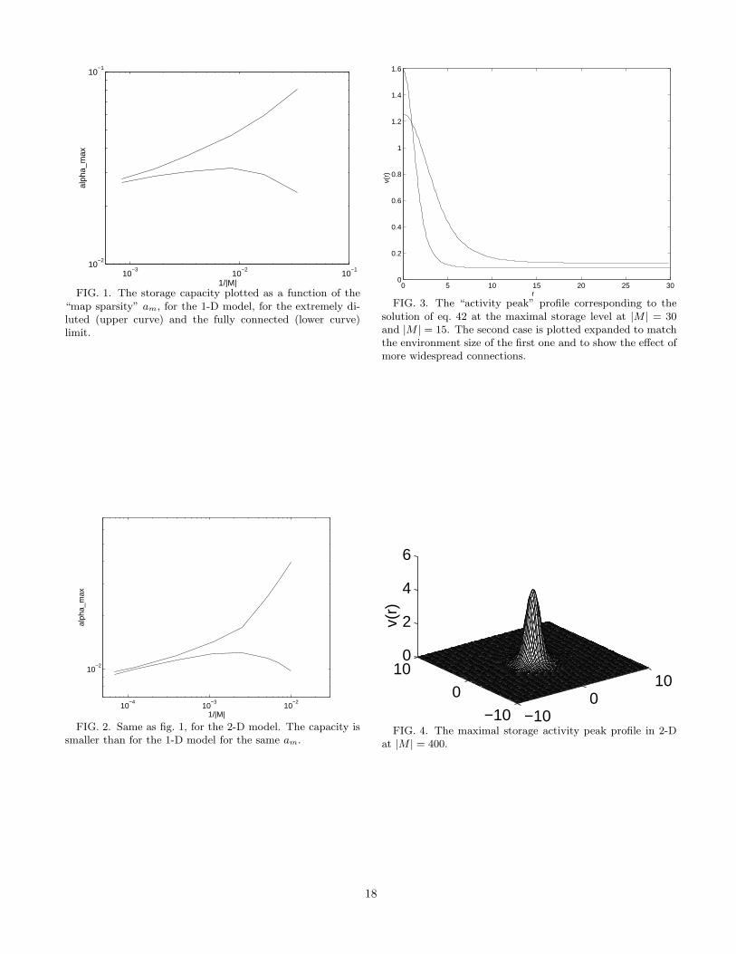
Eq. D9 can be solved numerically, an example is pro-vided in fig. 7, but a few features can be explored ana-lytically, in the neighborhood of ǫ = 0. r12 = 1, ǫ = 0

is a solution, but now consider what happens when ǫ in-creases.

Figure 7 approx. here

The derivatives of

D(r12, ǫ) = α〈〈K2〉〉g2

∫

dr

|M |Q(u(r), u(r + ǫ), r12) − r12

(D10)

with respect to ǫ and r12 must be taken into considera-tion. One has:

∂

∂ǫD(r12 = 1, ǫ = 0) = α〈〈K2〉〉g2

∫

dr

|M | ×

∂

∂yQ(x = u(r), y = u(r + ǫ), 1)u′(r) = 0, (D11)

∂2

∂ǫ2D(r12 = 1, ǫ = 0) < 0 (D12)

15

and

∂

∂r12D(r12 → 1, ǫ = 0) =

α〈〈K2〉〉g2

∫

dr

|M |Φ(u(r)) − 1 =

∫

dr

|M |Φ(u(r))

(∫

dr

|M |M(u(r))

)−1

− 1 (D13)

From eq. D12 it turns out that when the derivative ineq. D13 is greater than zero, the solution r12 = 1 disap-pears as one moves from ǫ = 1, but another solution isstill present so that

limǫ→0+

r12(ǫ) < 1. (D14)

Note that the condition

∂

∂r12D(r12 → 1, ǫ = 0) > 0

is equivalent to

Γ = gα|M |〈〈K2〉〉∫

M

dr u(r)v(r) < 0, (D15)

and the quantity Γ enters in the stability analysis con-siderations we sketched in sec. III C, at least for the 1-Dcase. Solutions with Γ > 0 are stable against inhibitionorthogonal fluctuations, so that it is likely that the possi-ble pathology implied by eq. D14 reflects an instability ofthe solution. We have always found numerically that forsolution corresponding to the maximal storage capacityand information, Γ > 0.

Once we know the joint probability distribution for z1

and z2, we can calculate the information we can extractabout the p.f.c. of a cell from two measurements of activ-ity, while the rat is standing in two positions at a distanceǫ, from all charts.

I2(ǫ) = α

∫

M

dr

|M |

∫ ++

Dz12

[

− 1

2(1 − r212)

(z21 + z2

2 − 2r12z1z2) −

log(

∫

M

dr′

|M | exp(

− 1

2(1 − r212)

[(u(r′) − u(r) + z1)2 + (u(r′ + ǫ) − u(r + ǫ) + z2)

2

−2r12(u(r′) − u(r) + z1)(u(r′ + ǫ) − u(r + ǫ) + z2)])

)]

+2

∫ +−

Dz12

[

log(

∫

z′

2>u(r+ǫ)

dz′22π

exp(

− 1

2(1 − r212)

(z21 + z′2

2 − 2r12z1z′2))

)

− log(

∫

M

dr′

|M |

∫

z′

2>u(r′+ǫ)

dz′2 exp(

− 1

2(1 − r212)

[(u(r′) − u(r) + z1)2 + (u(r′ + ǫ) − u(r + ǫ) + z′2)

2

−2r12(u(r′) − u(r) + z1)(u(r′ + ǫ) − u(r + ǫ) + z′2)])

)

]

+

∫ −−

Dz12

[

log(

∫

z′

1>u(r),z′

2>u(r+ǫ)

dz′1dz′2

2π√

1 − r212

exp(

− 1

2(1 − r212)

(z′12+ z′2

2 − 2r12z′1z

′2))

)

− log(

∫

M

dr′

|M |

∫

z′

1>u(r′),z′

2>u(r′+ǫ)

dz′1dz′2

2π√

1 − r212

exp(

− 1

2(1 − r212)

[(u(r′) − u(r) + z′1)2 + (u(r′ + ǫ) − u(r + ǫ) + z′2)

2

−2r12(u(r′) − u(r) + z′1)(u(r′ + ǫ) − u(r + ǫ) + z′2)])

)

]

. (D16)

The minus signs (−) beside the integration signs meanthat respectively the first, or the second condition deter-mining the integration intervals in eq. D8 are reversed.The first term in the sum accounts for the contributioncoming from measurement in which both activity valuesare positive. The second term is the contribution frommeasurements in which one value is zero and the otheris positive. The third term comes from measurements inwhich both values are zero.

For ǫ = 0, I2 = I1, since the two measures are identical.

For large ǫ one has I2 ∼ 2I1, because the noise decor-

relates and because in general the two measures will givenon-zero results in distinct regions of the environment.The behavior of I2 as a function of ǫ is exemplified infigure 8. We define as “information correlation length”the value lI of ǫ for which

I2 − I1 = fI1, (D17)

where f is a fixed fraction, say 0.95. Note that this quan-tity We may say that measurements of activity with therat in two positions at a distance lI give independent

16

information.

Figure 8 approx. here

This allows us to define as the stored information Is

the quantity

Is = I1|M |ldI

, (D18)

that is, sampling the activity of a cell |M|

ldI

times, with the

animal spanning a lattice with size lI , we may effectivelyadd up the information amounts we get from each singlesample, as if they were independent.

[1] D. Amit, Modeling Brain Function. (Cambridge Univer-sity Press, New York, 1989).

[2] M. Tsodyks and T. Sejnowski, Proceedings of the thirdworkshop on Neural Networks: from Biology to High En-ergy Physics - International Journal of Neural Systems 6

Supp., 81 (1994).[3] R. Muller, J. Ranck, and J. Taube, Current Opinion in

Neurobiology 6, 196 (1996).[4] D. Touretzky and A. Redish, Hippocampus 6, 247 (1996).[5] K. Gothard, W. Skaggs, and B. McNaughton, Journal of

Neuroscience 16, 8027 (1996).[6] A. Treves, Physical Review A 42, 2418 (1990).[7] B. Derrida, E. Gardner, and A. Zippelius, Europhysics

Letters 4, 167 (1987).[8] A. Treves, Journal of Physics A: Math. Gen. 24, 327

(1991).[9] A. Samsonovich and B. McNaughton, Journal of Neuro-

science 17, 5900 (1997).[10] A. Georgopoulos, R. Kettner, and A. Schwartz, Journal

of Neuroscience 8, 2928 (1988).[11] M. Wilson and B. McNaughton, Science 261, 1055

(1993).

17

10−3

10−2

10−1

10−2

10−1

1/|M|

alph

a_m

ax

FIG. 1. The storage capacity plotted as a function of the“map sparsity” am, for the 1-D model, for the extremely di-luted (upper curve) and the fully connected (lower curve)limit.

10−4

10−3

10−2

10−2

1/|M|

alph

a_m

ax

FIG. 2. Same as fig. 1, for the 2-D model. The capacity issmaller than for the 1-D model for the same am.

0 5 10 15 20 25 300

0.2

0.4

0.6

0.8

1

1.2

1.4

1.6

r

v(r)

FIG. 3. The “activity peak” profile corresponding to thesolution of eq. 42 at the maximal storage level at |M | = 30and |M | = 15. The second case is plotted expanded to matchthe environment size of the first one and to show the effect ofmore widespread connections.

−100

10

−10

0

100

2

4

6

v(r)

FIG. 4. The maximal storage activity peak profile in 2-Dat |M | = 400.

18

10−3

10−2

10−1

10−2

10−1

100

1/|M|

I_m

ax

FIG. 5. The maximal storable information per synapse, asa function of 1/|M |.

−5 −4 −3 −2 u_max 0 u* 2 3 4 5 0

5

10

15

20

25

u

U(u

)

FIG. 6. The “potential” function U(u) defined by eq. B7and entering the differential equation eq. B6. Solutions withu′(0) = 0 and u(0) = u0, with umax < u0 < u∗ are oscillating.The solution with u0 = u∗ is the one we seek, asymptoticallyapproaching umax as r → ∞.

0 10 20 300

0.2

0.4

0.6

0.8

1

epsilon

r_12

FIG. 7. The r12 function plotted as a function of the dis-tance between the two p.f.c.s, ǫ in the |M | = 30 case.

0 5 10 15 20 25 300.008

0.01

0.012

0.014

0.016

0.018

epsilon

I2

FIG. 8. The I2 function plotted as a function of the dis-tance between the two p.f.c.s, ǫ in the |M | = 30 case. Notethat lI , with f = 0.95 (see eq. D17) would be approximately3.5. This is seen not to change much when |M | is varying(not shown).

19