Attractor Tempos for Metrical Structures

February 3, 2015 Journal of Mathematics and Music ”Attractor Tempos for Metrical Structures”

To appear in the Journal of Mathematics and Music

Vol. 00, No. 00, Month 20XX, 1–25

Attractor Tempos for Metrical Structures

Mark Gotham, University of Cambridge, UK, [email protected]

(Received 00 Month 20XX; final version received 00 Month 20XX)

Through new mathematical modelling based on experimentally-substantiated principles

of cognitive science, this paper provides robust principles for identifying “attractor tempos”

which optimise the salience of metrical structures. This sheds lights on core musical phenom-

ena such as the inclination towards particular tempos in given metrical contexts, the use of

(non-optimal) tempos as a source of expressive tension in music, and even what it means for

music to be “fast” or “slow” in the first place.

The study begins with necessary preliminaries from music theory and the cognitive sci-

ences. The limitations of standard music-theoretic accounts of metre, such as in Lerdahl

and Jackendoff (1983), are outlined and a quantification of pulse salience is presented. This

quantification is used to nuance the music-theoretic account by bringing it more in line with

what is known about pulse perception: metres continue to be defined additively in terms of

combined levels; however, each of those levels is weighted on the basis of its salience. The

combination of constituent (individual) pulse saliences is taken as a representation of a met-

rical structure’s salience (hereafter “metrical salience”), and the criteria for optimising that

metrical salience value are set out. Attractor tempos can be deduced from the number of

metrical levels represented and their proportional relationship in largely simple, categorical

ways; however, the nature of those categories is intriguingly counter-intuitive.

This paper does not purport to set out a comprehensive model of metrical listening, but

simply to identify the core principles which are necessarily involved in establishing attractor

tempos. The (limited) dependence of those principles on the initial modelling parameters is

discussed. Furthermore, there is no prescription of “correct” tempos in this paper, instead

the attractors represent a set of defaults against which to select tempos for expressive effect.1

Keywords: Music; mathematics; metre; timing; tempo; modelling; pulse salience.

00A65, 97M80

1. Introduction / music theory

The basic hierarchies of common metres are well known to musicians and have been

described in a number of ways by music theorists. Figure 1 reproduces an example from

Lerdahl and Jackendoff (1983), in which metrical structure is represented by a stream of

1Please note that there is also an online supplement to this article, providing a subsidiary data table, and further

mathematical working. I gratefully acknowledge those scholars who read and commented on this earlier drafts of

this work, especially Justin London, Thomas Fiore, and two anonymous reviewers for the Journal of Mathematics

and Music.

1


21

3

v~

0 r~

L,

m ~J

.~

Downloaded by [University of Cambridge] at 04:30 13 September 2013

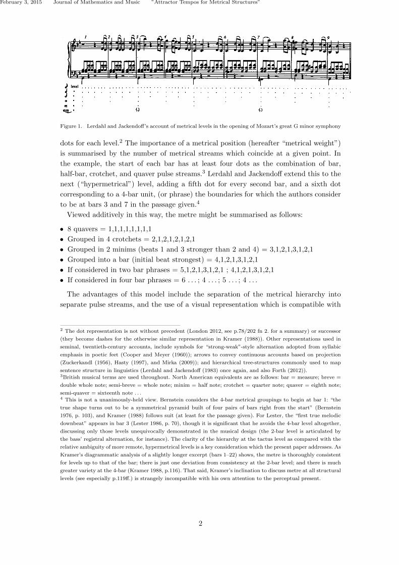
Figure 1. Lerdahl and Jackendoff’s account of metrical levels in the opening of Mozart’s great G minor symphony

dots for each level.2 The importance of a metrical position (hereafter “metrical weight”)

is summarised by the number of metrical streams which coincide at a given point. In

the example, the start of each bar has at least four dots as the combination of bar,

half-bar, crotchet, and quaver pulse streams.3 Lerdahl and Jackendoff extend this to the

next (“hypermetrical”) level, adding a fifth dot for every second bar, and a sixth dot

corresponding to a 4-bar unit, (or phrase) the boundaries for which the authors consider

to be at bars 3 and 7 in the passage given.4

Viewed additively in this way, the metre might be summarised as follows:

• 8 quavers = 1,1,1,1,1,1,1,1

• Grouped in 4 crotchets = 2,1,2,1,2,1,2,1

• Grouped in 2 minims (beats 1 and 3 stronger than 2 and 4) = 3,1,2,1,3,1,2,1

• Grouped into a bar (initial beat strongest) = 4,1,2,1,3,1,2,1

• If considered in two bar phrases = 5,1,2,1,3,1,2,1 ; 4,1,2,1,3,1,2,1

• If considered in four bar phrases = 6 . . . ; 4 . . . ; 5 . . . ; 4 . . .

The advantages of this model include the separation of the metrical hierarchy into

separate pulse streams, and the use of a visual representation which is compatible with

2 The dot representation is not without precedent (London 2012, see p.78/202 fn 2. for a summary) or successor

(they become dashes for the otherwise similar representation in Kramer (1988)). Other representations used in

seminal, twentieth-century accounts, include symbols for “strong-weak”-style alternation adopted from syllabic

emphasis in poetic feet (Cooper and Meyer (1960)); arrows to convey continuous accounts based on projection

(Zuckerkandl (1956), Hasty (1997), and Mirka (2009)); and hierarchical tree-structures commonly used to map

sentence structure in linguistics (Lerdahl and Jackendoff (1983) once again, and also Forth (2012)).3British musical terms are used throughout. North American equivalents are as follows: bar = measure; breve =

double whole note; semi-breve = whole note; minim = half note; crotchet = quarter note; quaver = eighth note;

semi-quaver = sixteenth note . . .4 This is not a unanimously-held view. Bernstein considers the 4-bar metrical groupings to begin at bar 1: “the

true shape turns out to be a symmetrical pyramid built of four pairs of bars right from the start” (Bernstein

1976, p. 103), and Kramer (1988) follows suit (at least for the passage given). For Lester, the “first true melodic

downbeat” appears in bar 3 (Lester 1986, p. 70), though it is significant that he avoids the 4-bar level altogether,

discussing only those levels unequivocally demonstrated in the musical design (the 2-bar level is articulated by

the bass’ registral alternation, for instance). The clarity of the hierarchy at the tactus level as compared with the

relative ambiguity of more remote, hypermetrical levels is a key consideration which the present paper addresses. As

Kramer’s diagrammatic analysis of a slightly longer excerpt (bars 1–22) shows, the metre is thoroughly consistent

for levels up to that of the bar; there is just one deviation from consistency at the 2-bar level; and there is much

greater variety at the 4-bar (Kramer 1988, p.116). That said, Kramer’s inclination to discuss metre at all structural

levels (see especially p.119ff.) is strangely incompatible with his own attention to the perceptual present.

2


Figure 2. Two notational contexts for the “same” material in the third movement of Martinu’s Les Fresques

de Piero della Francesca. Left: the opening of the movement (in 6/8); right: the recapitulation of that opening

material six bars before rehearsal mark 36 (in 3/4 at almost exactly twice the tempo).

pulse projection. The focus on metrical levels also implicitly accounts for some metrical

commonalities which are obfuscated by musical notation. Consider the two moments

from the third movement of Martinu’s Les Fresques de Piero della Francesca which are

reproduced in Figure 2. There is a clear correspondence between the two moments: in

the second version, the note lengths are twice as long, but the tempo is twice as fast and

so the aural, musical result is nearly-identical to the original. Although they may look

different, the two notational contexts are formally equivalent, distinguished only by the

different associations they may invoke with respect to particular styles and epochs.5

But what if one of these contexts used an extra metrical level at the fast-end (such as

demi-semi-quavers in the latter)? We would then have a different starting point for count-

ing dots, and so the equivalent metrical levels would be offset such that non-equivalent

levels are related by the same number of dots. The addition of a metrical level is sure

to have some effect, but not so great as to undermine the clear equivalence between

corresponding levels in this case. Clearly this is a weakness.

The dot-wise system leads to strange correspondences of this kind in even the simplest

examples. For instance, it attributes the same value to the bar-level in 3/4 as to the

half-bar-level value in 4/4 (“3” in the examples given):

• 6 quavers = 1,1,1,1,1,1

• Grouped in 3 beats = 2,1,2,1,2,1

• Grouped into a bar (initial beat strongest) = 3,1,2,1,2,1.

This may allude to a valid way of viewing the relative structural weights – that metres

with more internal levels require more definition than those with fewer – but it is unlikely

that two clearly different metrical streams could be satisfactorily represented by the same

value. This problem can be addressed in another direction by normalising the bar-level

weightings at a certain value instead of the fastest pulse,6 however that approach merely

re-locates the problem rather than solving it.

Ultimately, the integer values are too simplistic to deal with these core aspects of

metre. This is not so much a criticism of Lerdahl and Jackendoff whose object is only to

depict a hierarchy, but it is important to improve that model in line with these critiques

because it is used as the basis for quantitative applications in which those values assume

a significance.7

5Other examples of this particular notational equivalence include the codas to the first and third movements of

Prokofiev’s First Violin Concerto. Again, the “same” music is notated in 6/8 and 3/4, respectively.6This is the approach taken by David Meredith in his 1996 thesis where “the metric strength of any location that

is the initial location of a bar is 1” (Meredith 1996, pp. 214–5).7See, for instance, Chapter 13 of Toussaint (2013). The “Generative Theory of Tonal Music” (in which this model

3


To summarise, Lerdahl and Jackendoff’s model successfully incorporates accounts of

metrical structure and the use of metrical levels. This is enough for it to predict the equiv-

alence of the two Martinu moments. The main shortcoming is that it fails to address the

other obvious commonality: tempo. A related weakness is Lerdahl and Jackendoff’s im-

plicit assumption that the various metrical levels are equally salient and important to the

metrical experience. Even their own Mozart analysis (shown above) hints at the fact that

this is not valid: the highest hypermetrical level is equivocal, while the primary counting

levels are perfectly clear.8 Again a consideration of tempo improves this situation.

This paper address those problems by combining the viable aspects of the music-

theoretic approach with core principles from the cognitive sciences to develop a new

model of metrical weight and salience. This leads to the development of a heuristic for

optimising the salience of any simple metre, and the identification of those optimised

“attractor tempos” along with the metrical categorisation to which those tempos are

linked. Concluding comments include a discussion of the limited extent to which altering

the initial modelling parameters affects the final results: most of the core observations

are relatively unconstrained by those specifics.

2. Individual pulse salience

One reason for the equivocal 4-bar hypermetre in the Mozart example may be that pulse

streams are not equally discriminable across the spectrum. The literature9 suggests that:

• there is a preference for pulses around 100 beats per minute (hereafter “bpm”) which

equates to an interonset interval (IOI) of 0.6 seconds;

• pulses shorter than 0.1 seconds cease to be metrically useful; and

• the upper limit for what can be grouped as a single (metrical) unit is approximately

6 seconds.

These three values give us a truer sense of the relative salience of pulses at different

tempos, and the means to construct a perceptually-minded model of metrical weight.

The exact values for all three of these reference points are contested, especially that

of the upper limit which varies considerably according to the information content: for

our purposes, the musical context. This upper limit is closely related to the important

categorical boundary of the “psychological present” – a time-span during which informa-

tion is in current, active use rather than stored (and thus past)10 – and as John Michon

appears) is a high-profile, oft-cited work and this is obviously not the first refinement of the model to be proposed.

For another refinement to a too-simplistic (“strongly reduced”) aspect of the metrical part, see London’s “weak

reduction hypothesis” (London 1997).8This debate is taken up in other scholars’ analyses of this passage as discussed.9See London 2012, p.27ff. for a summary of the literature in support of these values.10James (1890) is frequently cited as the earliest exposition, though his first reference to the “specious present”

is to cite a section from Clay 1882, as the originator of the term and concept (p. 609). James proceeds to cite

empirical experimental data conducted by Wundt, Dietze, Estel, and Mehner concerning relevant temporal values

before proceeding to a more speculative, original examination of the idea. Clay defines the “specious present” as

distinct from the fleeting, ungraspable “real present” as well as from the “obvious past”(Clay 1882, pp. 167–9).

Subsequent landmarks include Michon (1978)’s review of the existing psychological literature at that time; Clarke

4


has it, “Because the present is so highly adaptive, no fixed parameter values can be ex-

pected to describe it adequately” (Michon 1978, p. 89). However, although we may lack

a definitive set of values to work with, we nevertheless have a sufficiently clear picture of

the phenomenon to create a model which demonstrates its heuristic value by illuminat-

ing important, generalisable information about maximising cumulative pulse salience in

metrical structures.11

In developing a suitable model of pulse interonset interval x against salience S, we

require a smoothly continuous curve to account for all x-values; the x-value at which the

curve peaks (indicating maximal salience) to be at 0.6 seconds; and the salience to be

negligible in the range x < 0.1 and x > 6.0. We may achieve this using the Gaussian

function12 given by equation (1), and illustrated in Figure 3.

S = exp

(−(log(x )− log(µ)

)22σ2

). (1)

0.1 0.2 0.5 1.0 2.0 5.00.0

0.2

0.4

0.6

0.8

1.0

Pulse IOI in Seconds x

Puls

eSal

ienc

eS

Figure 3. A quantitative model for pulse salience based on experimentally-derived values discussed in the text.

A logarithmic x-scale is used here to give a symmetrical decay from the peak at x = 0.6

to negligibly low values for 0.06 (below 0.1) and 6.0 seconds. The y-axis range is set from

0 – 1 arbitrarily, according to mathematical convention,13 and the width is given by σ =

0.3 to result in the y-values becoming negligibly low at the desired position. The value

of σ is an important issue which is discussed further in section 5.3. So, for µ = 0.6 and

σ = 0.3,

S = exp

(−(log(x/0.6)

)20.18

)(2)

(1987)’s ground work for an analytical application; and the use of the “present” in prominent theories of metre

such as Hasty (1997).11Further discussions in this paper includes the nature of existing data and models for pulse salience in the

context of the approach taken here (section 3), the generalisability of the principles which the present paper

deduces (section 6.1), and some prospects for further empirical study (section 6.2).12Despite the suggestive names “µ” and “σ,” this is not primarily intended as a probabilistic model.13The Gaussian constant is 1 and therefore omitted.

5


3. On the choice of distribution, the cognitive-scientific background, and

the aims of the present heuristic

These equations do not constitute the first or only mathematical model of pulse percep-

tion, they merely outline the approach taken in this paper as part of developing a new

heuristic for understanding the factors involved in optimising metrical salience. Although

developed independently, the logarithmic-Gaussian model of pulse salience used in this

paper is also used by Parncutt (1994) to describe a “kind of band-pass filter, admitting

only pulse sensations that lie within a given range of periods” (p. 438). Alternative ac-

counts include van Noorden and Moelants (1999)’s “effective resonance curve”, shown in

Figure 4 adapting to a range of data sets of potential relevance to the notion of pulse

salience (including Parncutt’s).14 Significant here is the relative agreement among the

various data sets and models.

Figure 4. Taken from van Noorden and Moelants (1999), this figure provides a graphic insight into competing

claims on pulse salience. Two sets of the authors’ newly-collected data which are thought to be good indications

of a tempo preference dominate the fast end of the spectrum (jagged lines). These are compared with versions

of van Noorden and Moelants’ model tailored to fit that data (“grey solid line”), as well as the data of Parncutt

(1994) (the “dashed line”), Handel and Oshinsky (1981) (the “thick black solid line”), and Vos (1973) (dotted line

which is the outlier for reasons of experimental design).

Van Noorden and Moelants’ alternative model appears to be based on the “Cauchy”

(“Lorentz”) distribution (though nowhere is that quite stated).15 This distribution has

assumed an importance in physics as the solution to the motion of a “driven damped

harmonic oscillator” and van Noorden and Moelants hypothesise that the physiological

basis of tempo perception works in an analogous way. That is not to say that there is

necessarily any physical oscillator literally involved, but rather that the physics for this

principle provides a useful model for the extent of the collective firing of neurons.

14A version of this figure showing only van Noorden and Moelants’ data and model can be found in Leman

2003(Leman 2003, sec.3.4.3).15The “resonance period” and “damping constant” variables conceptually correspond to some extent with the µ-

and σ-values used as part of the Gaussian distribution here and in Parncutt (1994). Incidentally, the normal and

Cauchy distributions are related in that the latter is given by the x/y ratio of the former.

6


While we must be cautious about asserting connections between the separate discover-

ies of physiological and behavioural studies, the recent literature continues to strengthen

the case for the eminently intuitive parallels among aspects relevant to the study of pulse

preference.16 In the broadest terms, it is currently thought that oscillations in neural fir-

ing adapt in order to regularly preempt anticipated moments of interest.17 This leads to

a distribution of neural resources that favours moments which are expected to contain

important information. That distribution equates to a relative amplification of the signal

which facilitates the processing of information received at that time.

However, while there are promising developments in understanding the neural corre-

lates to pulse salience, and no shortage of excellent studies on its behavioural manifesta-

tions, it is not likely that so general a principle can ever be comprehensively modelled in

the abstract, independent of context.18 How would a truly context-independent model

of pulse salience be constructed? What data should be used? Should it be taken from

physiological studies of ensemble neural firing, from behavioural studies, or from some

combination of both? Among these, what kinds of experiments are the most generalis-

able? In order to ensure ecological validity for musical listening, should we limit ourselves

to those few studies which make use of real musical examples?19 If so, then a first prob-

lem is that real music involves many metrical levels, mostly in fully-binary configurations

such as 4/4. This makes them an interesting point of comparison for the final results of

this model (models of “metrical salience”, particularly of simple binary metres),20 but

inappropriate as a starting model of individual pulse preference. Secondly, musical genre

has been shown to have an effect,21 so a representative balance of musical repertories

would be needed.22

One inevitably runs into large methodological questions of this kind, and (equally

inevitably) falls short of a truly generalisable representation. However, as this paper will

show, only a very approximate handle on “pulse salience” is needed to make significant

observations about the principles behind the emergence of certain (“attractor”) tempos

which appear to optimise salience for whole categories of metres. Accordingly, this paper

does not attempt to address those larger issues. It remains agnostic about what “pulse

salience” exactly is, about the distribution which best accounts for it, and about the

nature of the brain’s (and indeed the body’s) involvement.23 Rather, this paper seeks

merely to make musical use of what is – however approximately – known.

In keeping with the appropriate level of accuracy for modelling this phenomenon, and

16For summaries of relevant, recent literature, see London (2012) Chapter 3, Repp and Su (2013) especially

Sections 1.5 and 4, and Calderone et al. (2014). Calderone et al. include an extremely useful, up-to-date overview

of relevant, recent work including a tabular summary of both the behavioural and neurological effects that have

been observed in connection with oscillatory entrainment.17For instance, Cravo et al. (2013) demonstrate the entrainment of alpha band oscillations in the visual cortex in

response to a visual stimulus.18Volk (2008) (discussed below) represents a recent computational line of inquiry that is most promising for

defining the phase and period of metrical levels of that musical context.19These include van Noorden and Moelants (1999), Toiviainen and Snyder (2003), and McKinney and Moelants

(2006). See London 2012, p.27ff. for a discussion of ecological validity in this context.20The data would have to be separated or re-collected according to metrical structure and level usage.21As demonstrated in van Noorden and Moelants (1999), and McKinney and Moelants (2006).22See London (2013) for a discussion of what that might look like in practice.23See, for instance, Trainor et al. (2009).

7


the theoretical-speculative approach accordingly taken here, the mathematical model

used to represent pulse salience in this paper is the simplest, most parsimonious available

(the logarithmic Gaussian in equation (1)). This allows for results to be expressed clearly,

in basic categorical terms (particularly in relation to the µ-value); in the context of this

heuristic, categories are more useful than a large collection of apparently disassociated

numbers. Section 6.1 sets out how changes to the initial model affect the numerical results

generated, but (importantly) that the core principles advanced here remain intact.

In short, the hypothesis that humans prefer pulses in a certain range has been tested.

The outcomes of those tests include various results which do not perfectly align with one

another but which collectively point to a general agreement about the kind of shape that

should be used for a model of pulse salience in the abstract. This paper makes use of

such a model to develop a new model of metrical salience which has explanatory value

in terms of tempo choice. In turn, the new model also represents a testable hypothesis

for the cognitive sciences (discussed in section 6.2).

4. Combined periodicities (metre)

The model of individual pulse salience in Figure 3 outlines a central peak, but musical

intuition and theoretical accounts of the metrical hierarchy tell us that metrical positions

corresponding to longer durations have greater metrical weight. These principles are

perfectly compatible as long as metre is modelled as the sum of several periodicities: a

modelling assumption which this paper shares with scholars like Lerdahl and Jackendoff

and Parncutt alike.24 Modelling metre in this way necessarily preserves the positive

correlation between duration and metrical weight while also leaving room to include a

weighting of the constituent pulses’ importance. Here, the salience S of each pulse x is

modelled by equation (1), and the weight of a metrical position is given by the sum of

the saliences for the pulses which coincide there (as defined by the metrical hierarchy).

For instance, in a metrical structure consisting exclusively of groupings by 2 (a “binary

metre”), the available pulse rates consist of all binary multiples and divisions of the

tactus with an x-value between 0.1 and 6 seconds (the “metrical window” in London’s

terminology).25 Where the crotchet pulse IOI = 0.6 seconds (100bpm), this includes:

• 0.15 seconds (the semi-quaver),

• 0.3 seconds (the quaver),

• 0.6 seconds (the crotchet),

• 1.2 seconds (the minim),

• 2.4 seconds (the semi-breve: the length of the bar if in 4/4),

• and 4.8 seconds (the breve: a 2-bar unit in 4/4).

Assuming that all of these available levels are used, the metrical weight of any position

24“The salience of a perceived meter may be estimated by summing the saliences of the consonant pulse sensations

of which it is composed” (Parncutt 1994, p.455).25London uses the terms “temporal envelope” as well as “metrical window” for this range (London 2012, p.27ff.),

while Parncutt speaks of an “existence region” (Parncutt 1994, p. 436). “Metrical window” is the term used in

this paper.

8


is given by the sum of S-values for all pulses coinciding there. For the weight associated

with the crotchet-level in this example, we sum the S-values corresponding to x = 0.6

(the crotchet level itself) as well as x = 0.3 and 0.15 (the faster levels); for the weight

associated with the 4/4 bar-level, we add to that sum S(1.2) and S(2.4). This may

continue to any further “hyper-metrical” levels within the acceptable range (only one in

this case). The values for this example are summarised in Table 1 (and also compared

with three other important examples in the Online Supplement to this paper).

Pulse Stream (IOI in seconds) 0.15 0.3 0.6 1.2 2.4 4.8

Individual pulse salience 0.133 0.604 1 0.604 0.133 0.011

Cumulative (metrical) salience 0.133 0.738 1.738 2.342 2.476 2.487Table 1. Quantified pulse salience and metrical weight for the levels of an example binary metre. Individual pulse

salience is given by equation (2), and metrical weightings are given by the sum of the longest pulse involved and

all faster pulse constituents. This is given by equations (3) for full-represented binary metres and (4) for any other

circumstance. In this example, note the symmetry of S values about S(0.6), the central peak of the (individual)

pulse salience curve used.

Equation (3) generalises this principle for any position in a binary metre. For any

metrical position, let x now stand for the duration it represents (the time that elapses

before the next position of equal or higher metrical value). A binary metre’s metrical

weight B is given by the sum of the saliences S of the constituent metrical levels: pulse

IOIs of x/2n for natural numbers n. Because intervals outside the 0.1–6 second range

have negligible salience, we can restrict the range of the sum to values of n satisfying

0.1 < x/2n < 6 for n ≥ 0. It can be shown that the maximum value of n satisfying this

restriction is given by N = b(log x− log 0.1)/log 2c. B may therefore be expressed as:

B =

N∑n=0

exp

(−(log(x/2n)− log(0.6)

)20.18

), 0.1 < x < 6. (3)

So this system adds a value for each metrical level (just as with Lerdahl and Jack-

endoff’s dots), but weights the relative importance of each constituent level according

to its salience. The importance of the respective levels can be seen in the left-hand ex-

ample of Figure 5 which sets out the metrical hierarchy corresponding to the example

in Table 1. Strong-weak alterations can be easily observed for some levels, while for

the others they are barely noticeable. For instance, the strong-weak distinction between

x = 0 and x = 4.8 on the one hand (S(0) = S(4.8) = 2.487), and x = 2.4 on the other

(S(2.4) = 2.476), can hardly be seen on Figure 5.

Once again, observations of this kind shed light on analytical matters such as the hy-

permetrical ambiguity in the Mozart example above. While strong and weak alternations

are easily discerned at the most salient tactus level, it is often much harder to deduce

relative metrical weight at higher levels. It may be that the Classical practice of varying

phrase lengths while keeping the tactus levels constant is reliant on that fact.26

26In the Mozart example, quaver, crotchet, minim, and semi-breve hierarchies are all evident from the notation

and the musical cues. The breve (2-bar) level is absent from the notation and is almost consistently used; while

the 4-bar level is considerably more varied still. Refer again to Kramer’s diagram for a diagrammatic analysis of

9


1 2 3 4Time

0.5

1.0

1.5

2.0

2.5

Weight

level for 4/4).3 Note that the exclusion of the least com-mon temporal positions represents a more conservativeanalysis – the uniformly rare use of the positions of lowermetric stability might otherwise artificially inflate corre-lations between the tonal and metric hierarchies.Table 5 shows the results of correlating the resulting

12 (pitch class) by 16 (metric stability) tonal-metricmatrices across composer, separately for each time

signature and modality. Values are the average corre-lation coefficients of each composer with all othercomposers. All Table 5 values below .70 are the resultof cells with the minimum possible small sample size(N pieces ! 2).The strikingly high inter-composer tonal-metric cor-

relations of Table 5 motivated including additionalcomposers, including some from more modern compo-sitional periods; we chose Schubert, Brahms, Liszt, andScriabin (see Appendix B for the list of included piecesof these composers). These data are not included in theearlier analyses because our corpus had too few pieces ofthese composers for valid inter-composer comparisons.

FIGURE 2. Metric hierarchy values: frequency of occurrence and Palmer-Krumhansl (1990) goodness of fit ratings, all standardized to maximum of 1.(a) 2/4 time signature, (b) 3/4 time signature, (c) 4/4 time signature, (d) 6/8 time signature.

3We used the 16 most common temporal positions from all timesignatures even if it did not correspond to the sixteenth note level (e.g.,3/4) because we were sorting by stability as indexed by frequency ofoccurrence rather than beat strength.

Tonal-Metric Hierarchy 259

Figure 5. Left: a stem chart for metrical weight, taking the example of two bars of 4/4 metre at crotchet = 100

bpm (IOI = 0.6 seconds) as set out in Table 1. Right: Prince and Schmuckler (2014)’s quantification of metrical

position usage in a large sample of music in 4/4 (within metre only – giving fewer levels). This is included to

demonstrate the similar distribution patterns between the present, theoretical model based on pulse salience, and

the objective evidence of note usage. “PK1990” refers to Palmer and Krumhansl (1990)’s landmark study of the

metrical hierarchy, which includes a small corpus study of its own.

Encouragingly, the new theoretical stem chart describes similar hierarchical patterns

not only to traditional accounts of metre in a general sense, but also to corpus studies

of metrical position usage. For comparison, Figure 5 also includes such an example from

Prince and Schmuckler (2014), specifically for position usage in 4/4 contexts over a large

sample of works.27 Note the relatively large difference between the quaver and crotchet

levels (compare positions 3,7,11,15 with 5,13), but the much lesser difference between

those of the minim and semi-breve (positions 9 and 1).28

5. Optimising metrical salience; identifying attractor tempos

We now turn to the primary goal of optimising “metrical salience” for all simple metres

represented by any number of (consecutive) metrical levels, and thus identifying the

“attractor tempos” for those metres (the x-value at which the metrical salience of that

metre is optimised). Metrical salience is operationally defined here by the combined

saliences of all the pulse streams present in the metrical structure (the highest single

metrical weight value). If we represent the fastest pulse as x, and all higher levels by the

relevant multipliers (px, qx, rx . . . ), then the highest metrical weight value which can be

obtained is given by

M =∑

n=1, p, q, r, ...

exp

(−(log(nx/µ)

)22σ2

). (4)

bars 1–22 (Kramer 1988, p.116).27Position usage provides another possible basis for quantifying metrical weight. See also Volk (2008) for a context-

specific “quantification of the note’s [metrical position’s] metric importance [usage]” (p.99) that is un-constrained

by the notated metre, extending to hypermetrical levels, and dissonant configuration, for instance.28It would be particularly interesting to test the effect of tempo on position usage.

10


The function B(x) for binary metres is one case of M(x). Optima are represented by

local maxima of this sum which are located at zeros of the first derivative.29

As Parncutt (1994) briefly observes, this cumulative salience of a high metrical level

(his “aggregate salience”) is not necessarily maximised by the tempo which optimises the

salience of the individual pulse (p. 438). Parncutt suggests this as a reason why subjects

in tapping studies are drawn to other tempos when tapping in specified groupings: to

faster tempos for larger groupings.30 This appears to indicate a desire to balance the

various pulse levels involved, maximising the combination rather than any individual

pulse.

This section sets out a model for optimising metrical salience in the context of any

simple metrical structure based on binary and ternary grouping at each consecutive,

structural level. While it is possible to sustain up to six metrical levels within the metrical

window, fewer are present in the majority of musical contexts (and certainly the tapping

tasks that dominate the literature). This study therefore accounts for the number of

levels represented as well as the proportional structure; level usage does indeed turn out

to be an important factor.

5.1. An exhaustive list of metrical structures

Table 2 provides a comprehensive list of every possible metrical structure based on con-

secutive levels of 2- and 3-grouping which fall within the metrical window defined. The

metrical window constraint dictates that the single-unit level can be combined with fur-

ther levels up to a limit of 60-units.31 Therefore, this table includes metres with 54-unit

levels, but not those with 64 (the two values of 2m ∗ 3n which are closest to 60). Metres

are defined by their proportional structure and level usage (not by time signatures). For

instance, “binary metres” with grouping by 2 at each level comprise the whole first block;

any binary time signature (“2/4,” “4/4,” . . . ) could refer to any one of these structures.

The first column lists examples of time signatures which express each of the metrical

levels involved, (along with the corresponding notational values in brackets). Some of

those signatures representing many metrical levels are rare, but this does not necessarily

mean that the metrical structure itself is also rare. For instance, “48/16” could be notated

as a simple binary metre with triplets at the fastest level. However, it is worth noting

that as the number of 3-levels increases the metrical structures do indeed become rarer.

There is not even a standard symbol for a 9-unit value. We would have to invent a

dotted(dotted(unit)) as distinct from a double-dotted one (7 units). Question marks in

29The necessary mathematics are supplied in the Online Supplement.30See Fraisse (1956, 1982) and Vos (1973). Fraisse tested the spontaneous tempo for tapping in metrical groups.

His results indicate a preference for faster rates when tapping in 3s (IOI = 0.42seconds), and faster still when in

4s (0.37seconds) (Fraisse 1956, p. 15). This matches Vos (1973), a test of subjective grouping at different tempos

in which participants were given pulses with IOIs of 0.15, 0.2, 0.3, 0.4, and 0.8 seconds and a choice of grouping

in 2, 3, 4, 5, 6, 7, or 8. Grouping by 2 was most attractive for IOIs of 0.8 seconds, by 3 at 0.4seconds, and by 4

at 0.3 seconds. That said, binary groupings (2, 4, 8) far outperformed any contender, accounting for 63/75 of the

whole study. Both results indicate a correlation between the size of metrical grouping and the tempo preferred:

the larger the group, the faster the tempo.31The lower limit, 0.1 seconds, multiplied by 60 units equals 6 seconds (the upper limit).

11


the table indicate this situation.

The second and third columns set out respectively the pulse length for each level

(in units) and the proportional multipliers between consecutive levels (invariably 2 or

3). These columns also introduce notation used in the remainder of the article: sets of

numbers in angle brackets denote the pulse length for each level (in ascending order

starting with 1), and the proportional schemes between those consecutive levels are

given in square brackets. For instance, [3,2,2] corresponds to the proportional scheme

in 〈1, 3, 6, 12〉. If “1” refers to the quaver level, then “3” refers to that of the dotted

crotchet, and so on.

The following, “x-max” column deals with the 0.1 < nx < 6.0 seconds constraint. The

lower limit for x is always set by 0.1, but the maximum depends on the metrical structure:

the slowest pulse level must be no slower than 6 seconds. The x-max is therefore given by

6 seconds divided by the number of units in the slowest pulse level. The x-max column

thus gives a sense of how constrained each metre is by the values. Clearly, the longer

the longest pulse level, the narrower the x-range. For instance, metres with a 54x pulse

level can only fit all of those levels within the metrical window if 0.1 < x < 0.1. These

constraints illustrate one of the difficulties associated with sustaining all the levels of

such a metre.

The “Attractor” column lists the attractor tempos in the form of the x-values which

optimise M(x) for each metre; and the final column provides some related information

about that optimal value. This includes information about the categorisation of metres

into groups which may be optimised by the same x-value (a “categorical attractor”).

This is the main result of the present article and the subject of the discussion which

follows. A brief taxonomy of metrical types will facilitate that discussion.

• “Binary metres” consist exclusively of 2-unit groupings between consecutive levels;

• “ternary metres” include at least one level of 3-unit grouping (all non-binary metres);

• it will be useful to distinguish between metres employing an odd number of metrical

levels (“odd metres”) and those with an even number (“even”); and finally

• “symmetrical” structures have a symmetrical pattern of ratios between consecutive

levels, for instance [3,2,3]. All symmetrical metres are identified on Table 2.

5.2. Odd and Even symmetrical metres

We begin with first principles and the simplest possible metres. The model of individual

pulse salience in Figure 3 represents the optimising curve for a trivial metre of only one

pulse level. Clearly, the optimal x-value for this “metre” is µ, the same as for the pulse.

If we add a second metrical level to this pulse, then the optimum changes. Figure

6 shows the interaction of x and 2x pulse streams: a binary metre represented by two

metrical levels. The image on the left shows the individual pulses x and 2x as two versions

of Figure 3, as well as their combined curve. This combined M(x) curve shows how the

combination is optimised by a compromise between the two individual pulses such that

x = µ/√

2 = 0.424 seconds: a value which positions the two metrical levels at equal

distance from the µ (0.6 seconds) as shown by the right-hand image of Figure 6. The

12


Example Pulse lengths Proportions x-max Attractor (x) Additional information

1/4 (c only) 〈1〉 (n/a) 6 0.6 Symmetrical: x = µ

2/4 (c, m) 〈1, 2〉 [2] 3 0.424 Symmetrical: x = µ/√

2

2/4 (q, c, m) 〈1, 2, 4〉 [2,2] 1.5 0.3 Symmetrical: 2x = µ

2/4 (sq, q, c, m) 〈1, 2, 4, 8〉 [2,2,2] 0.75 0.212 Symmetrical: 2x = µ/√

2

4/4 (sq, q, c, m, sb) 〈1, 2, 4, 8, 16〉 [2,2,2,2] 0.375 0.15 Symmetrical: 4x = µ

4/2 (sq, q, c, m, sb, b) 〈1, 2, 4, 8, 16, 32〉 [2,2,2,2,2] 0.1875 0.106 Symmetrical: 4x = µ/√

2

3/4 (c, dm) 〈1, 3〉 [3] 2 0.346 Symmetrical: x = µ/√

3

3/8 (sq, q, dc) 〈1, 2, 6〉 [2,3] 1 0.352

6/8 (q, dc, dm) 〈1, 3, 6〉 [3,2] 1 0.170

3/4 (sq, q, c, dm) 〈1, 2, 4, 12〉 [2,2,3] 0.5 0.277

6/8 (sq, q, dc, dm) 〈1, 2, 6, 12〉 [2,3,2] 0.5 0.332; (0.0904) Symmetrical about 2x = µ/√

3

12/16 (sq, dq, dc, dm) 〈1, 3, 6, 12〉 [3,2,2] 0.5 0.108

3/2 (sq, q, c, m, dsb) 〈1, 2, 4, 8, 24〉 [2,2,2,3] 0.25 0.204

6/4 (sq, q, c, dm, dsb) 〈1, 2, 4, 12, 24〉 [2,2,3,2] 0.25 (0.274) Secondary peak (0.454) also off

12/8 (sq, q, dc, dm, dsb) 〈1, 2, 6, 12, 24〉 [2,3,2,2] 0.25 (0.0546) Secondary peak (0.331) also off

24/16 (sq, dq, dc, dm, dsb) 〈1, 3, 6, 12, 24〉 [3,2,2,2] 0.25 (0.0737) As fast as possible

3/1 (sq, q, c, m, sb, db) 〈1, 2, 4, 8, 16, 48〉 [2,2,2,2,3] 0.125 (0.147) (48x = 7.03)

6/2 (sq, q, c, m, dsb, db) 〈1, 2, 4, 8, 24, 48〉 [2,2,2,3,2] 0.125 (0.203) Secondary peak (0.0227) also off

12/4 (sq, q, c, dm, dsb, db) 〈1, 2, 4, 12, 24, 48〉 [2,2,3,2,2] 0.125 (0.275; 0.0273) Symmetrical about 4x = µ/√

3

24/8 (sq, q, dc, dm, dsb, db) 〈1, 2, 6, 12, 24, 48〉 [2,3,2,2,2] 0.125 (0.0369) Secondary peak (0.331) also off

48/16 (sq, dq, dc, dm, dsb, db) 〈1, 3, 6, 12, 24, 48〉 [3,2,2,2,2] 0.125 (0.0512) As fast as possible

9/16 (sq, dq, ?) 〈1, 3, 9〉 [3,3] 0.6 0.2 Symmetrical: 3x = µ

9/8 (sq, q, dc, ?) 〈1, 2, 6, 18〉 [2,3,3] 0.3 (0.349) (18x = 6.28)

18/16 (sq, dq, dq, ?) 〈1, 3, 6, 18〉 [3,2,3] 0.3 0.141 Symmetrical: 3x = µ/√

2

18/16 (sq, dq, ?, ?) 〈1, 3, 9, 18〉 [3,3,2] 0.3 (0.0573) As fast as possible

9/4 (sq, q, c, dm, ?) 〈1, 2, 4, 12, 36〉 [2,2,3,3] 0.16 (0.277) As fast as possible

18/8 (sq, q, dc, dm, ?) 〈1, 2, 6, 12, 36〉 [2,3,2,3] 0.16 (0.0733) Secondary peak (0.332) also off

18/8 (sq, q, dc, ?, ?) 〈1, 2, 6, 18, 36〉 [2,3,3,2] 0.16 (0.349; 0.0287) Symmetrical about 6x = µ

36/16 (sq, dq, dq, dc, dm, ?) 〈1, 3, 6, 12, 36〉 [3,2,2,3] 0.16 0.1 Symmetrical: 6x = µ

36/16 (sq, dq, dq, ?, ?) 〈1, 3, 6, 18, 36〉 [3,2,3,2] 0.16 0.136 Secondary peak off lower limit

36/16 (sq, dq, ?, ?, ?) 〈1, 3, 9, 18, 36〉 [3,3,2,2] 0.16 (0.0362) As fast as possible

27/16 (sq, dq, ?, ?) 〈1, 3, 9, 27〉 [3,3,3] 0.2 0.149; (0.0895) Symmetrical about 3x = µ/√

3

27/8 (sq, q, dc, ?, ?) 〈1, 2, 6, 18, 54〉 [2,3,3,3] 0.1 (0.349) As slow as possible

54/16 (sq, dq, dc, ?, ?) 〈1, 3, 6, 18, 54〉 [3,2,3,3] 0.1 (0.141) As slow as possible

54/16 (sq, dq, ?, ?, ?) 〈1, 3, 9, 18, 54〉 [3,3,2,3] 0.1 (0.0474) As fast as possible

54/16 (sq, dq, ?, ?, ?) 〈1, 3, 9, 27, 54〉 [3,3,3,2] 0.1 (0.0191) Secondary plateau (c. 0.2) also off

Table 2. All possible metrical structures based on grouping in 2s and 3s with details concerning the optimal

x-value. Parentheses enclose solutions which fall outside the acceptable range. In the example column, the abbre-

viations used are: “s” for “semi-”, “d” for “dotted-”, “q” for “quaver”, “c” for “crotchet”, “m” for “minim”, and

“b” for “breve”. The x-values are expressed in terms of the µ where possible, and given to 3 significant figures

(3s.f.) elsewhere. Rounding to 3 significant figures applies throughout this article.

mathematics is explained in footnote 32. That equidistance generates an equal salience

for S(x) and S(2x) which results in a higher combined M(x) value than would have been

achieved by optimising either pulse individually at the expense of the other.

If we add a third binary level to give the metrical structure 〈1, 2, 4〉, then we return to a

situation where the optimal M(x) value is given by optimising an individual pulse value

at the µ. Specifically, 〈1, 2, 4〉 is maximised by centring the metrical structure such that

the middle 2x level is individually optimised at the µ (x = µ/2) as shown in Figure 7.

The correspondence between 〈1〉 and 〈1, 2, 4〉 as distinct from 〈1, 2〉 represents the

second main categorical distinction invoked above, between “odd” and “even” sym-

metrical metres. Odd and even metres are all centred and balanced in this way: odd

32 Because we are dealing with a logarithmic scale, the distance between two x-values (x1 and x2) is measured

by log(x1/x2). If x1 and x2 are consecutive metrical levels on either side of the µ, then x2/µ = µ/x1. It is also

the case here that x2 = 2x1 and so 2x1/µ = µ/x1, so x21 = µ2/2, and x1 = µ/√

2. For a µ value of 0.6, this gives

x = 0.424 seconds.

13


M HxL=SHxL+SH2xLSHxLSH2xL

0.1 0.2 0.5 1.0 2.0 5.00.0

0.5

1.0

1.5

Pulse I.O.I.

Salie

nce

0.1 0.2 0.5 1.0 2.0 5.00.0

0.2

0.4

0.6

0.8

1.0

Pulse IOI

Salie

nce

Figure 6. Left: the interaction of two pulse streams in a ratio of 1:2 with a peak at x = µ/√

2 = 0.424 seconds (3

s.f.). Right: this x-value along with the corresponding 2x on the curve for individual pulse salience, demonstrating

their equal distance from the mean.

SHxL+SH2xL+SH4xL

0.1 0.2 0.5 1.0 2.0 5.00.0

0.5

1.0

1.5

2.0

Pulse IOI

Salie

nce

0.1 0.2 0.5 1.0 2.0 5.00.0

0.2

0.4

0.6

0.8

1.0

Pulse IOI

Salie

nce

Figure 7. Left: the interaction of three pulse streams in a ratio of 1:2:4 with a peak at x = µ/2 = 0.3. Right: this

x-value along with the corresponding values for 2x and 4x on the curve for individual pulse salience, demonstrating

their symmetrical centring on the mean.

metres by positioning the central level at the peak; even metres by positioning the cen-

tral two levels equidistant from the peak on either side. For many symmetrical metres,

these centred forms optimise the metrical salience; however, this is conditional on the

σ-value: an important parameter to which we now turn.

5.3. The sigma value

The measurement of distance from µ can be generalised for two metrical levels in any

n-relation: x and nx are equidistant from µ when x = µ/√n. However, that value cannot

be generalised as an optimal solution because the shape of the combined curve is heavily

dependent on the σ-value: for larger values of n, and smaller values of σ, the model

outputs a pair of optima nearer to the optima of the individual curves (x = µ and

nx = µ respectively).

In Figure 8, the x and 2x combination of Figure 6 is reproduced (left) along with an

alternative form using a smaller σ-value (right) for comparison. As the σ-value is smaller,

the individual S(x) curves are narrower, sufficiently so in this case that their combined

M(x) curve separates into two distinct peaks, giving two equal maxima. For reference,

the line at x = 0.424 is reproduced: this is the optimal x-value in the left-hand (large

σ) condition of Figure 8, but is a local minimum in the right-hand (small σ) case. As

the σ-value is increased, the two separate peaks converge, leading to the single, central

14


maximum as in the left-hand case (and Figure 6).

M HxL=SHxL+SH2xLSHxLSH2xL

0.1 0.2 0.5 1.0 2.0 5.00.0

0.5

1.0

1.5

Pulse I.O.I.

Salie

nce

SHxL+SH2xLSHxLSH2xL

0.1 0.2 0.5 1.0 2.0 5.00.0

0.2

0.4

0.6

0.8

1.0

Pulse IOI

Salie

nce

Figure 8. Left: S(x), S(2x), and S(x)+S(2x) (the left part of Figure 6 reproduced); right: the same with narrower

individual curves, leading the optimisation curve to split into two separate peaks. Note the lower salience values

(y-scale).

At σ = 0.3, the combination of x and 3x is optimised by x = µ/√

3, but the combination

of x and 4x is not optimised by x = µ/√

4. The σ-value has been set at 0.3 partly because

this is a thoroughly appropriate benchmark for that categorical shift. At Parncutt’s σ-

value of “typically about 0.2” (Parncutt 1994, p.438), the combination of x and 3x already

separates into distinct regions, yielding the choice of high and low optima (0.152 and 0.590

respectively). That the categorical shift should occur here is inconsistent with intuition

and both Fraisse and Vos’ results (discussed above). However, that the categorical shift

should occur before the combination of x and 4x is positively an asset as it gives meaning

to the commonly invoked formal requirement that such a combination ought to include

an intervening 2x level. Were the σ-value large enough to maximise x and 4x at x =

µ/√

4 = µ/2 then it would make no difference whether the 2x level is included or not

(〈1, 2, 4〉 is an odd, symmetrical binary metre also optimised by x = µ/2). As x = µ/2 is

not the optimum for this σ-value, the 2x level is essential to the metrical structure.

Cases which lack a single optimum represent the prioritisation of one pulse over an-

other. The effect is magnified when metrical levels are added as whole sets of pulses

may group in “sub-metres” that are easier to handle than the whole. Frequently, the

“optimal” solutions to these metres suggest an x-value for which peripheral pulse levels

fall outside the metrical window. Once again, this models the difficulty of sustaining all

the levels of a large metre and the concomitant tendency to concentrate on optimising

a subset at the expense of the peripheral levels. Often, these subsets stand to generate

a much higher total M(x) value than any legitimate solution to the larger metres could.

While the σ-value has to be extremely low to affect the outcomes for any binary metres,

ternary metres are more susceptible, as the greater ratio makes the peripheral levels con-

comitantly remote. We therefore turn specifically to consider ternary metres and larger

combinations.

5.4. Ternary metres

For the present σ-value, all binary metres are optimised by the categorical x-values of

nx = µ for odds, and nx = µ/√

2 for evens where nx refers to the metrical level at or

15


immediately below the µ. Symmetrical ternary metres may be optimised in the same

categorical ways, but they are more susceptible to splitting into separate peaks.

For symmetrical odd ternary metres, the σ-value used here is such that nx = µ

maximises 〈1, 3, 6, 12, 36〉 [3,2,2,3], and 〈1, 3, 9〉 [3,3], but not 〈1, 2, 6, 18, 36〉 [2,3,3,2]. The

metre [2,3,3,2] splits into separate peaks not so much because of the number of levels

(the same as for [3,2,2,3]), but more due to the preponderance of 3-grouping in the centre

which thus separates two 〈1, 2〉 metres. This is an important consideration which applies

to many ternary metres, symmetric or otherwise.

Like even binary meters, symmetrical even ternary metres may be optimised

by x-values such that their central levels are equidistant from the µ. Here, we must

distinguish between metres with a binary grouping at their centre, and those with a

ternary grouping. The central levels are equidistant from µ when the faster pulse stream

nx equals µ/√

2 for binary groupings (as discussed) and µ/√

3 for ternary.33 Figures 6 and

9 represent the centre of these two metrical structures to which any symmetrical patterns

of levels may be added. Figure 6 sets out the binary relationship (nx and 2nx equidistant

from the µ), while Figure 9 sets out the ternary equivalent for the combination of nx

and 3nx including the optimum at nx = µ/√

3 = 0.346 seconds. For the present σ-value,

the metres 〈1, 3〉 [3] and 〈1, 3, 6, 18〉 [3,2,3] are optimised by the symmetrical centring,34

while 〈1, 2, 6, 12〉 [2,3,2], 〈1, 2, 4, 12, 24, 48〉 [2,2,3,2,2], and 〈1, 3, 9, 27〉 [3,3,3] are not. Once

again, it is partly the use of many metrical levels, but especially the preponderance of

3-groupings in the centre that causes this.

SHxL+SH3xLSHxLSH3xL

0.1 0.2 0.5 1.0 2.0 5.00.0

0.2

0.4

0.6

0.8

1.0

1.2

1.4

Pulse I.O.I.

Salie

nce

0.1 0.2 0.5 1.0 2.0 5.00.0

0.2

0.4

0.6

0.8

1.0

Pulse IOI

Salie

nce

Figure 9. Left: the interaction of two pulse streams in a ratio of 1:3 with a peak at x = µ/√

3 = 0.346 sec-

onds. Right: this x-value along with the corresponding value for 3x on the curve for individual pulse salience,

demonstrating their equal distance from the mean.

Table 2 includes all relevant values for these split symmetrical metres: the two paired

peak values are given in the “Attractor” column, and the symmetrical centre of these

peaks (the categorical attractor) is discussed in “Additional information”. For instance,

〈1, 2, 6, 12〉, is symmetrical and splits due to the ternary centre. Here, the optimal column

shows these two solutions (0.332 and 0.0904), while the “additional information” is that

they are equidistant from a categorical attractor at 2x = µ/√

3.

It is useful to keep sight of the categorical attractors because for a larger σ-value the

categorical attractor would be the optimum: the Mmax for split symmetrical metres is

33nx continues to refer to the metrical level at or immediately below the µ.34The metre [3,2,3] is the only even ternary metre with a binary centre that can exist within the metrical window.

16


conditional on the σ-value, while the categorical attractors are not. It is also important

not to rely unduly on the output optima because for large metres, the optimal tempo

which the equation outputs is frequently such that the peripheral metrical levels would

fall outside the metrical window. On table 2, parentheses enclose solutions which fall

outside the acceptable range. For instance, the metrical structure 〈1, 2, 4, 12, 24, 48〉 out-

puts two solutions equidistant from 4x = µ/√

3. The ternary separation of 〈1, 2, 4〉 from

〈12, 24, 48〉 means that the “optimum” is achieved by positioning one such binary trio

much nearer the peak positions (with the central value of those three near the mean),

leaving the other trio at unacceptably slow or fast rates.35 Clearly an “optimum” output

of that kind is not a solution to the problem of optimising saliences for the full metrical

structure. Rather, it highlights the difficulty of such metres, and the tendency for them

to decompose to other, simpler metres with fewer levels. Sub-optimal solutions can be

reached by tempos as close to the optimum as is allowable. Some of these are indicated

on Table 2 by phrases such as “as fast as possible.”

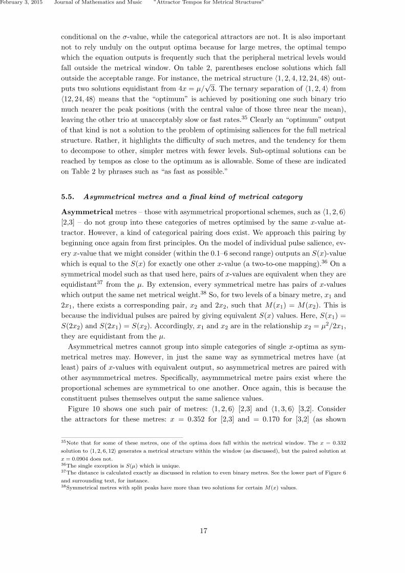
5.5. Asymmetrical metres and a final kind of metrical category

Asymmetrical metres – those with asymmetrical proportional schemes, such as 〈1, 2, 6〉[2,3] – do not group into these categories of metres optimised by the same x-value at-

tractor. However, a kind of categorical pairing does exist. We approach this pairing by

beginning once again from first principles. On the model of individual pulse salience, ev-

ery x-value that we might consider (within the 0.1–6 second range) outputs an S(x)-value

which is equal to the S(x) for exactly one other x-value (a two-to-one mapping).36 On a

symmetrical model such as that used here, pairs of x-values are equivalent when they are

equidistant37 from the µ. By extension, every symmetrical metre has pairs of x-values

which output the same net metrical weight.38 So, for two levels of a binary metre, x1 and

2x1, there exists a corresponding pair, x2 and 2x2, such that M(x1) = M(x2). This is

because the individual pulses are paired by giving equivalent S(x) values. Here, S(x1) =

S(2x2) and S(2x1) = S(x2). Accordingly, x1 and x2 are in the relationship x2 = µ2/2x1,

they are equidistant from the µ.

Asymmetrical metres cannot group into simple categories of single x-optima as sym-

metrical metres may. However, in just the same way as symmetrical metres have (at

least) pairs of x-values with equivalent output, so asymmetrical metres are paired with

other asymmmetrical metres. Specifically, asymmmetrical metre pairs exist where the

proportional schemes are symmetrical to one another. Once again, this is because the

constituent pulses themselves output the same salience values.

Figure 10 shows one such pair of metres: 〈1, 2, 6〉 [2,3] and 〈1, 3, 6〉 [3,2]. Consider

the attractors for these metres: x = 0.352 for [2,3] and = 0.170 for [3,2] (as shown

35Note that for some of these metres, one of the optima does fall within the metrical window. The x = 0.332

solution to 〈1, 2, 6, 12〉 generates a metrical structure within the window (as discussed), but the paired solution at

x = 0.0904 does not.36The single exception is S(µ) which is unique.37The distance is calculated exactly as discussed in relation to even binary metres. See the lower part of Figure 6

and surrounding text, for instance.38Symmetrical metres with split peaks have more than two solutions for certain M(x) values.

17


on the two graphs). The S-value equivalences here are: S(1 ∗ 0.352) = S(6 ∗ 0.170);

S(2 ∗ 0.352) = S(3 ∗ 0.170); and S(6 ∗ 0.352) = S(1 ∗ 0.170). The same equivalence holds

for any pair of x-values which are equidistant from their symmetrical centre39 at 0.245.

SHxL+SH2xL+SH6xL

0.1 0.2 0.5 1.0 2.0 5.00.0

0.5

1.0

1.5

Pulse IOI

Salie

nce

SHxL+SH3xL+SH6xL

0.1 0.2 0.5 1.0 2.0 5.00.0

0.5

1.0

1.5

Pulse IOI

Salie

nce

Figure 10. The interaction of three pulse streams in a ratio of 1:2:6 (left) and 1:3:6 (right) along with their optima

at x = 0.352 and 0.170 respectively which are equidistant from the line about which these curves are symmetrical

to one another, x = 0.245.

6. Generalisability and improvements

6.1. The initial modelling parameters’ effect on the final results

It has been stressed that the shape of the pulse salience curve used here is not intended to

be definitive, but only as a tool for the heuristic being developed. The initial modelling

data provides only approximate boundaries and a sense of the shape. The attractor

tempos are, of course, affected by changes to the core model of pulse salience and so it is

necessary to understand the nature of these prospective changes. Principal among these

are changes to the width σ or centre µ of the current distribution, use of an alternative

(asymmetrical) distribution, and the pursuit of a different definition of metrical salience.

The effect of the σ-value has been discussed amply in section 5.3 above and needs

no further comment here. Clearly, were the µ to be positioned at a faster or slower

position, the optima it generates for metres would all follow in the same direction by

logarithmic increments.40 One motivation for relocating the µ would be if the studies

that have given rise to the idea of 0.6 are considered to be flawed as representatives of

truly single-pulse metrical acts, and in fact indicative of a preferred solution to the 〈1, 2〉metre, for instance. Given the human tendency towards subjective rhythmisation, and

the dominance of binary metres, this is not a trivial matter to unpick.

While some alternative distribution models for salience have also been discussed, their

effect on the outcome merits further comment in terms of the model’s generalisability.

Within reasonable bounds, the principal observations of this model apply to all related

“bell-curve”-esque models. The nature of many pairings and equivalences will still hold,

though the exact symmetrical values will clearly not. Any change to the distribution

39The centre is equidistant from x = 0.352 and 0.170, at√

0.352 ∗ 0.170 = 0.245.40For instance, increasing the µ from 0.6 to 0.7 would increase the µ/

√2 value from 0.424 to 0.495.

18


would have two main effects. Firstly, asymmetry would mean all optimal tempos move in

the direction of the skew. For instance, an increased positive skewness – that is, a positive

skew even on a logarithmic scale – would shift all optima to faster pulses (shorter IOIs).41

Secondly, any change to the shape of the distribution would have a similar effect to the

width in that it would adjust the point at which metres decompose from single into

separate peaks that may not best serve the metre as a whole. An asymmetric model

would cause an asymmetric decomposition – affecting some metres more than others.

Nevertheless, the principal categorical observations hold true including the fact of this

decomposition and the variables which affect it: particularly the use of many metrical

levels, and the preponderance of 3-groupings in the centre. The model thus remains

widely applicable to more complex forms of the pulse salience model and provides a

simple, useful handle on the principles of metrical salience.

Finally, we turn to the notion of “metrical salience” itself, here defined by the combined

saliences of all the pulse streams present in the given structure: a value which also

represents the metrical weight for the highest level present. This is taken to be a value

worth optimising, though it is not the only conceivable measure of metrical salience. We

could perhaps take the combined weights for all metrical positions, but this value would

disproportionately favour optimising the lowest levels (which occur the most frequently).

More plausibly, some manner of weighting could be given to the metrical levels in play

according to the strength of their usage in the musical context. Computational models

such as Volk (2008) are extremely promising as models of metrical level usage in real

musical contexts (or at least digitised score representations thereof),42 though they tend

only to account for a restricted set of musical parameters (excluding changes of harmony

and orchestration, for instance). They also tend to remain agnostic on perceptual matters,

thus neglecting to address the issues explored here. Therefore, a combination of context-

specific level weighting with the present model of metrical salience is a very promising

prospect (if used with analytical common sense). The fact that the model advanced here

is already in broad agreement with the average frequency of metrical position usage (as

shown in Figure 5 above) is most encouraging.

6.2. Refinement of the model by cognitive and corpus testing

The previous section (6.1) discussed the fact that many of the core observations of this

model are relatively independent of the exact modelling values used. This justifies and

gives strength to the heuristic observations made. Nevertheless, it is clearly desirable to

test this model in order to hone its accuracy as far as realistically possible.

The model invites many kinds of empirical testing, particularly of the principal hy-

pothesis that each metrical context may be made relatively easy or difficult to engage

by the choice of tempo. Most simply, subjects may be presented with stimuli in different

metrical configurations, and invited either to assess whether they consider the example

to be “fast” or “slow”, or to independently select a preferred tempo for the extract in-

41This would be one effect of using the model from van Noorden and Moelants (1999), for instance.42See also the ‘pulse clarity measure’ in Lartillot, Toiviainen, and Eerola (2008)’s ‘MIR toolbox’.

19


dependently. According to the hypothesis, preference ratings would reflect the shapes of

the metrical salience curves for the metrical structure in question. Alternatively, sub-

jects could be required to synchronise with given tempo-metrical contexts, or to observe

timing perturbations contained therein; one would expect the performance to be best at

tempos nearest the attractors.

It would also be desirable to assess the hypotheses in relation to real musical practice

in addition to musically-impoverished experimental stimuli of questionable ecological

validity. Corpora of works and performances are an attractive source of evidence, though

that approach also comes with a number of methodological warnings. Firstly, as has been

emphasised throughout, the “attractor” tempos are designed only to model a default,

easiest practice, and certainly not the “correct” tempos for musical expression (which

is often reliant on a deliberate distancing from easy, normative practice). In short, non-

optimal “fast” and “slow” tempos are at least as common as “moderate” ones that align

with their attractor. Even a very large sample may provide more evidence of congregation

at the extremes than of the default, easiest practice modelled here. Secondly, the model

advanced in this paper places great store on the metrical structure and level usage as

determinants of tempo choice. Clearly then, any corpus used to assess this model would

need to include that information. This rules out studies like van Noorden and Moelants

(1999) which include only tempo data.43 Instead, this necessitates the use of advanced

music information retrieval techniques, such as in Volk (2008), discussed above.

7. Summary and exemplary musical applications

7.1. Summary

This paper began by setting out a quantification of pulse salience (section 2) to weight the

significance of each metrical level according to its salience. That model was then used to

develop a further model for metrical salience (section 4) which enabled the deduction of

general principles for optimising net pulse salience in simple metres (section 5) and thus

identifying “attractor” tempos to which those metres may be drawn. Metrical salience

values depend on the tempo, the metrical structure, and the number of levels represented.

All distinct metres have distinct metrical salience curves; however, there are three main

categories of structurally similar metres which may be optimised by the same attractor

tempo. Figure 11 summarises the family structure of these categories.

This structure is intriguingly divergent from traditional accounts of metrical categories.

Here, the primary criterion for metrical identity is not the customary distinction between

binary and ternary metres (2/4 versus 3/4, for instance), nor even the number of metri-

cal levels represented, but rather the presence or absence of a symmetrical proportional

scheme among the levels. All three categorical attractors for maximising metrical salience

exist within the class of symmetrical metres. Asymmetric metres do not group in metrical

categories of that kind, though equivalent pairs of asymmetric metres are related by the

43Though those results may illuminate aspects of the binary metrical circumstances which dominate most of the

genres studied there.

20


.

''ww

Symmetrical

ww &&

Asymmetrical

Odd

��

Even

xx &&nx = µ [2]

��

[3]

��

nx = µ/√

2 nx = µ/√

3

Figure 11. A flowchart for metrical categories relevant to optimising. The level at or immediately below µ which

optimises the metrical salience for metres in a category is given by nx; the multiplier n depends on the number of

levels in use. The grouping of the central level of symmetrical even metres is given by “[2]” and “[3]” at the lowest

level of the chart.

shape of their metrical salience curves. The categorical attractors for the symmetrical

metres are given at the bottom of Figure 11, and are shown in Figures 7, 6, and 9 respec-

tively. The width of the original pulse salience curve dictates the limit of applicability

for these categorical attractors (see section 5.3). Metres with a large number of metrical

levels, and especially those with ternary groupings in the centre are harder to sustain,

and more liable to “optimise” at values which prioritise some sub-structure rather than

the whole.

7.2. Musical illustrations: short, fundamental examples

The model is ultimately useful in so far as it is able to elucidate fundamental musical

considerations. By way of conclusion, this section provides some brief illustrations of how

the model appears to do so, and suggests avenues for future application.

At the heart of the model is the notion that adding a faster metrical level (further

level of subdivision) generates a slower optimal tempo to accommodate (and vice versa –

adding slow hypermetrical levels leads to a faster optimum). Figure 12 provides a simple

illustration of this principle which is also suggestive of a possible stylistic application. In

version a), the fastest pulse level involved is the crotchet. If this is changed to a dotted

rhythm as in version b), the quaver level becomes involved, giving a metrical structure

with a slower attractor tempo (assuming equal importance of the levels). In version

(c) the rhythm is double-dotted, invoking the semi-quaver level, leading to a new, even

slower optimal. This may contribute to an understanding of why (double-)dotted rhythms

have come to be associated with grand (slow) styles such as the “French overture”. For

instance, this example is taken from the opening of Mozart’s Cosı Fan Tutte in which

version (c) is the form used, (and in which that semi-quaver level is also used melodically,

21


not just in these opening tutti chords).

Figure 12. Three version of the same example, with additional metrical levels leading to slower attractor tempos.

This connects directly with some of the bases for tempo choice expressed by practising

musicians since at least Quantz and Kirnberger in the Eighteenth-Century.44 Throughout

Quantz’ account of tempo (paragraphs 55ff.), the suggested tempos are related to both

the metrical structure, and the fastest pulse-level used.45 Kirnberger similarly asserts

that the tempo for each dance is ‘determined by the metre and the note values that

are employed in it’, also focussing on the faster stream (p.375 [105]ff.). These are direct

precursors to the present, technical model of attractor tempos, (which also considers the

highest metrical level used as part of its formalisation).

The attractors enable even a principled definition of what it means for music to be

“fast” or “slow”. For instance, what do we mean when we describe Barber’s Adagio

for Strings as a “slow” piece? Well, the time signature is 4/2, implying a minim pulse

and the metrical levels used include at least the crotchet (the shortest note-value used),

minim, semi-breve, and breve. This combination is maximised by the µ/√

2 value, giving

a minim value of 0.424 seconds, (141 bpm). Yet, the tempo designation is molto adagio,

presumably referring to that minim pulse. The fastest metronome mark that could still

be considered adagio is about 75 bpm which equates to a 0.8 seconds IOI. This (fastest

plausible) tempo is shown in Figure 13 in which it falls to the right side of centre.

0.1 0.2 0.5 1.0 2.0 5.00.0

0.2

0.4

0.6

0.8

1.0

Pulse IOI

Salie

nce

Figure 13. A visual representation of what it means to be slow: the fastest plausible tempo for Barber’s Adagio).

Clearly even this is much slower than the (symmetrically centred) optimum. The use

of longer bars in the piece (5/2, 6/2), the possible addition of hypermetrical levels,

44Quantz and Kirnberger’s major treatises date from 1752 (‘Versuch einer Anweisung die Flote traversiere zu

spielen’) and 1776–9 (‘Die Kunst des reinen Satzes in der Musik’) respectively. See Quantz ((trans. / ed. E. R.

Reilly 1966) and Kirnberger ((trans. / ed. D. Beach and J. Thyme 1982) for the modern, translated editions with

commentary that are referenced here.45For instance, ‘each of the types of metre cited can be put into its proper tempo’; to do so ‘it is most important

to consider both the word indicating the tempo at the beginning of the piece and the fastest notes used in the

passage-work’ (paragraph 51ff., my emphasis).

22


and acknowledgement of “molto” adagio (as distinct from merely adagio) all further

this separation.46 The piece is necessarily slow for any realistic tempo within the range

prescribed; Barber’s notation instructs the performer to use a slow tempo, far from the

attractor. In short, “slowness” has a lot to do with absolute tempo, of course, but just

as much to do with the metrical structure: the Barber is slow exactly because it relies on

metrical levels above the minim tactus. The attractor tempos provide useful benchmarks

for assessing this.

This is one kind of insight concerning expressive deviation from a default (easiest)

range that the present model makes possible, (and note once again that we only need a

very approximate understanding of the best distribution for the shape of pulse salience

to make the observation). The example also emphasises for the last and final time the

difference between the “attractor” tempos set out here (representing a kind of default,

easiest practice) and the “correct” tempo for musical expression in a given context: clearly

this music derives much of its expressive beauty from its slowness.

Even if one were deliberately to seek out these attractor tempos wherever possible as

if they were correct, the vast majority of music changes metrical level usage – and often

also the metrical structure itself – within sections governed by the same tempo. Pulse

levels come and go and local changes such as hemiolas are used; each new structure

brings its own attractor tempo which aligns to greater or lesser extent with whatever

tempo is actually used in performance. This guarantees a play of tension-relaxation as

one moves between relatively optimised and non-optimised tempo-metrical alignments –

an expressive device which can now be articulated and assessed by means of the attractor

tempo model advanced here.47

References

Bernstein, Leonard. 1976. The Unanswered Question: Six Talks at Harvard. Cambridge, MA: Harvard

University Press.

Calderone, Daniel J., Peter Lakatos, Pamela D. Butler, and F. Xavier Castellanos. 2014. “Entrainment

of Neural Oscillations as a Modifiable Substrate of Attention.” Trends in Cognitive Sciences http:

//www.cell.com/trends/cognitive-sciences/abstract/S1364-6613(14)00048-5.

Clarke, Eric F. 1987. “Levels of Structure in the Organization of Musical Time.” Contemporary Music

Review 2 (1): 211–238. http://www.tandfonline.com/doi/abs/10.1080/07494468708567059.

Clay, Edmund R. 1882. The Alternative: A Study in Psychology. London: MacMillan and Co.

Cooper, Grosvenor, and Leonard Meyer. 1960. The Rhythmic Structure of Music. Chicago: University of

Chicago.

Cravo, Andre M., Gustavo Rohenkohl, Valentin Wyart, and Anna C. Nobre. 2013. “Temporal Expectation

Enhances Contrast Sensitivity by Phase Entrainment of Low-Frequency Oscillations in Visual Cortex.”

The Journal of Neuroscience 33 (9): 4002–4010.

Forth, James. 2012. “Cognitively-Motivated Geometric Methods of Pattern Discovery and Models of

Similarity in Music.” Ph.D. thesis. University of London.

Fraisse, Paul. 1956. Les Structures rythmiques. Louvain: Publications Universitaires de Louvain.

46Compare this with Kirberger’s characterisation of tempo adjectives as a means to “add or take away from the

fast or slow motion of the natural tempo” (p.377[107]) – the “attractor tempo” in this article’s terminology.47This idea is thoroughly developed in an analytical follow-up to the present article – Gotham (2014. Preprint) –

a tempo metrical analysis of the third movement of Brahms’ Second Symphony (forthcoming).

23

http://www.cell.com/trends/cognitive-sciences/abstract/S1364-6613(14)00048-5

http://www.cell.com/trends/cognitive-sciences/abstract/S1364-6613(14)00048-5

http://www.tandfonline.com/doi/abs/10.1080/07494468708567059


Fraisse, Paul. 1982. “Rhythm and Tempo.” In The Psychology of music, edited by Diana Deutsch. 149–

180. New York: Academic Press.

Gotham, Mark. 2014. Preprint. “‘Attractor Tempi’ in Brahms 2/III.” .

Handel, Stephen, and James Oshinsky. 1981. “The Meter of Syncopated Auditory Polyrhythms.” Per-

ception and Psychophysics 30 (1): 1–9. http://dx.doi.org/10.3758/BF03206130.

Hasty, Christopher. 1997. Meter as Rhythm. New York ; Oxford: Oxford University Press.

James, William. 1890. The Principles of Psychology. Vol. 2. London: MacMillan.

Kirnberger, Johann Philipp. (trans. / ed. D. Beach and J. Thyme 1982). Art of strict musical composition.

Music theory translation series; 4. New Haven: Yale University Press.

Kramer, Jonathan D. 1988. The Time of music: new meanings, new temporalities, new listening strategies.

New York ; London: Schirmer.

Lartillot, Olivier, Petri Toiviainen, and Tuomas Eerola. 2008. “A Matlab Toolbox for Music Information

Retrieval.” In Data Analysis, Machine Learning and Applications, edited by C. Preisach, H. Burkhardt,

L. Schmidt-Thieme, and R. Decker. Studies in Classification, Data Analysis, and Knowledge Organi-

zation. Springer-Verlag.

Leman, Marc. 2003. “Foundations of Musicology as Content Processing Science.” JMM: The Journal of

Music and Meaning 1.

Lerdahl, Fred, and Ray Jackendoff. 1983. A Generative Theory of Tonal Music. Cambridge, MA: The

MIT Press.

Lester, Joel. 1986. Rhythms of tonal music. Carbondale: Southern Illinois University Press.

London, Justin. 1997. “Lerdahl and Jackendoff’s ‘Strong Reduction Hypothesis’ and the Limits of Ana-

lytical Description.” In Theory Only 13 (1): 3–29.

London, Justin. 2012. Hearing in time: psychological aspects of musical meter. 2nd ed. Oxford: Oxford

University Press.

London, Justin. 2013. “Building a Representative Corpus of Classical Music.” Music Perception: An

Interdisciplinary Journal 31 (1): pp. 68–90. http://www.jstor.org/stable/10.1525/mp.2013.31.

1.68.

McKinney, Martin F., and Dirk Moelants. 2006. “Ambiguity in Tempo Perception: What Draws Listeners

to Different Metrical Levels?.” Music Perception: An Interdisciplinary Journal 24 (2): 155–166. http:

//www.jstor.org/stable/10.1525/mp.2006.24.2.155.

Meredith, David. 1996. “The Logical Structure of an Algorithmic Theory of Tonal Music.” Ph.D. thesis.

University of Oxford.

Michon, John A. 1978. “The Making of the Present: a Tutorial Review.” In Attention and Performance,

Vol. VII edited by J. Requin. Hillsale, New Jersey: Erlbaum.

Mirka, Danuta. 2009. Metric manipulations in Haydn and Mozart: chamber music for strings, 1787-1791.

Oxford: Oxford University Press.

Palmer, Caroline, and Carol Krumhansl. 1990. “Mental Representations for Musical Meter.” Journal of

Experimental Psychology: Human Perception and Performance 16 (4): 728–741.

Parncutt, Richard. 1994. “A Perceptual Model of Pulse Salience and Metrical Accent in Musical

Rhythms.” Music Perception: An Interdisciplinary Journal 11 (4): 409–464. http://www.jstor.org/

stable/40285633.

Prince, Jon B., and Mark A. Schmuckler. 2014. “The Tonal-Metric Hierarchy: A Corpus Analysis.” Music

Perception: An Interdisciplinary Journal 31 (3): pp. 254–270. http://www.jstor.org/stable/10.

1525/mp.2014.31.3.254.

Quantz, Johann Joachim. (trans. / ed. E. R. Reilly 1966). On playing the flute. London: Faber.

Repp, Bruno, and Yi-Huang Su. 2013. “Sensorimotor Synchronization: A Review of Recent Research

(2006 - 2012).” Psychonomic Bulletin and Review 20 (3): 403–452. http://dx.doi.org/10.3758/

s13423-012-0371-2.

Toiviainen, Petri, and Joel Snyder. 2003. “Tapping to Bach: Resonance-Based Modeling of Pulse.” Music

Perception 21 (1): 43–80.

Toussaint, Godfried. 2013. The Geometry of Musical Rhythm. CRC Press.

Trainor, Laurel J., Xiaoqing Gaoa, Jing jiang Leia, Karen Lehtovaaraa, and Laurence R. Harris. 2009.

24

http://dx.doi.org/10.3758/BF03206130

http://www.jstor.org/stable/10.1525/mp.2013.31.1.68




http://www.jstor.org/stable/40285633

http://www.jstor.org/stable/40285633



http://dx.doi.org/10.3758/s13423-012-0371-2

http://dx.doi.org/10.3758/s13423-012-0371-2


“The Primal Role of the Vestibular System in Determining Musical Rhythm.” Cortex 45 (1): 35–43.

van Noorden, Leon, and Dirk Moelants. 1999. “Resonance in the Perception of Musical Pulse.” Journal

of New Music Research 28 (1): 43–66.

Volk, Anja. 2008. “Persistence and Change: Local and Global Components of Metre Induction using

Inner Metric Analysis.” Journal of Mathematics and Music 2 (2): 99–115. http://www.tandfonline.

com/doi/abs/10.1080/17459730802312399.

Vos, P. 1973. Waarneming van metrische toonreeksen. Nijmegen: Stichting Studentenpers.

Zuckerkandl, Victor. 1956. Sound and symbol: music and the external world. London: Routledge.

25



Attractor Tempos for Metrical Structures

Documents

Transcript of Attractor Tempos for Metrical Structures