Conditions for the emergence of spatially asymmetric retrieval states in an attractor neural network
11
CEJP 3(3) 2005 409–419 Conditions for the emergence of spatially asymmetric retrieval states in an attractor neural network Kostadin Koroutchev 1, 2∗ , Elka Korutcheva 3, 4 1 Departamento de Ingenier´ ıa Inform´ atica, Universidad Aut´ onoma de Madrid, 28049 Madrid, Spain 2 Institute for Computer Systems, Bulgarian Academy of Sciences, 1113, Sofia, Bulgaria 3 Departamento de F´ ısica Fundamental, Universidad Nacional de Educaci´ on a Distancia, c/Senda del Rey, No 9, 28080 Madrid, Spain 4 G. Nadjakov Institute of Solid State Physics, Bulgarian Academy of Sciences, 1784, Sofia, Bulgaria Received 15 January 2005; accepted 29 April 2005 Abstract: In this paper we show that during the retrieval process in a binary symmetric Hebb neural network, spatially localized states can be observed when the connectivity of the network is distance-dependent and a constraint on the activity of the network is imposed, which forces different levels of activity in the retrieval and learning states. This asymmetry in the activity during retrieval and learning is found to be a sufficient condition to observe spatially localized retrieval states. The result is confirmed analytically and by simulation. c Central European Science Journals. All rights reserved. Keywords: Neural networks, spatial localized states, replica formalism PACS (2000): 64.60.Cn, 84.35.+i, 89.75.-k, 89.75.Fb 1 Introduction In a recent publication [1] it was shown that using linear-threshold model neurons, the Hebb learning rule, sparse coding and distance-dependent asymmetric connectivity, spa- * E-mail: [email protected] - 10.2478/BF02475647 Downloaded from PubFactory at 08/01/2016 08:20:28AM via free access
Transcript of Conditions for the emergence of spatially asymmetric retrieval states in an attractor neural network
CEJP 3(3) 2005 409–419
Conditions for the emergence of spatially asymmetric
retrieval states in an attractor neural network
Kostadin Koroutchev1,2∗, Elka Korutcheva3,4
1 Departamento de Ingenierıa Informatica,Universidad Autonoma de Madrid,28049 Madrid, Spain2 Institute for Computer Systems,Bulgarian Academy of Sciences,1113, Sofia, Bulgaria3 Departamento de Fısica Fundamental,Universidad Nacional de Educacion a Distancia,c/Senda del Rey, No 9, 28080 Madrid, Spain4 G. Nadjakov Institute of Solid State Physics,Bulgarian Academy of Sciences,1784, Sofia, Bulgaria
Received 15 January 2005; accepted 29 April 2005
Abstract: In this paper we show that during the retrieval process in a binary symmetric
Hebb neural network, spatially localized states can be observed when the connectivity
of the network is distance-dependent and a constraint on the activity of the network is
imposed, which forces different levels of activity in the retrieval and learning states. This
asymmetry in the activity during retrieval and learning is found to be a sufficient condition
to observe spatially localized retrieval states. The result is confirmed analytically and by
simulation.c© Central European Science Journals. All rights reserved.
Keywords: Neural networks, spatial localized states, replica formalism
PACS (2000): 64.60.Cn, 84.35.+i, 89.75.-k, 89.75.Fb
1 Introduction
In a recent publication [1] it was shown that using linear-threshold model neurons, the
Hebb learning rule, sparse coding and distance-dependent asymmetric connectivity, spa-
∗ E-mail: [email protected]
- 10.2478/BF02475647Downloaded from PubFactory at 08/01/2016 08:20:28AM
via free access
410 K. Koroutchev, E. Korutcheva / Central European Journal of Physics 3(3) 2005 409–419
tially asymmetric retrieval states (SAS) can be observed. This asymmetric states are
characterized by a spatial localization of the activity of the neurons, described by the
formation of local bumps.
Similar results have been reported in the case of a Hebb binary model for associative
neural network [2]. The observation is intriguing, because all components of the network
are intrinsically symmetric with respect to the positions of the neurons and the retrieved
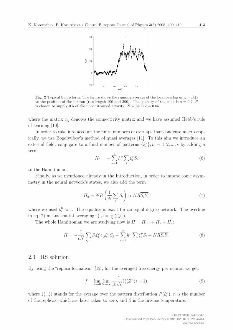
state is clearly asymmetric. An illustration of SAS in a binary network is presented in
Fig.2.
In parallel to the present investigation, extensive computer simulations have been
performed in the case of integrate and fire neurons [3], where the formation of bumps was
also reported. These results are in agreement with our previous results [2] that networks
of binary neurons do not show bumpy retrieval solutions when the stored and retrieved
patterns have the same mean activity.
The biological reason for this phenomenon is based on the transient synchrony that
leads to recruitment of cells into local bumps, followed by desynchronized activity within
the group [4],[5].
When the network is sufficiently diluted, say less then 5%, then the differences between
asymmetric and symmetric connectivity are minimal [6]. For this reason we expect that
the impact of the asymmetric connectivity will be minimal and the asymmetry need not
be considered as a necessary condition for the existence of SAS, as is confirmed in the
present work.
There are several factors that possibly contribute to the SAS in model network.
In order to introduce the spatial effects in neural networks (NN), one essentially needs
measures of distance and topology between the neurons, and to impose a distribution of
the connections that is dependent on the topology and distances. The major factor to by
which spatially asymmetric activity can be observed is of course the spatially dependent
connectivity of the network. Actually this is an essential condition, because given a
network with SAS, by applying random permutation to the enumeration of the neurons
one will obviously achieve states without SAS. Therefore, the topology of the connections
must depend on the distance between the neurons.
Due to these arguments, a symmetric and distance-dependent connectivity for all
neurons is chosen in this study.
We consider an attractor NN model of Hebbian type formed by N binary neurons
{Si}, Si ∈ {−1, 1}, i = 1, ..., N , storing p binary patterns ξµi , µ ∈ {1...p}, and we assume a
symmetric connectivity between the neurons cij = cji ∈ {0, 1}, cii = 0. cij = 1 means that
neurons i and j are connected. We regard only connectivities in which the fluctuations
between the individual connectivity are small, e.g. ∀i∑
j cij ≈ cN , where c is the mean
connectivity.
The learned patterns are drawn from the following distribution:
P (ξµi ) =
1 + a
2δ(ξµ
i − 1 + a) +1 − a
2δ(ξµ
i + 1 + a),
where the parameter a is the sparsity of the code. Note that the notation is a little bit
- 10.2478/BF02475647Downloaded from PubFactory at 08/01/2016 08:20:28AM
via free access
K. Koroutchev, E. Korutcheva / Central European Journal of Physics 3(3) 2005 409–419 411
different from the usual one. By changing the variables η → ξ + a and substituting in
the above equation, one obtains the usual form for the pattern distribution in the case of
sparse code [7].
Later in this article we show that when symmetry between the retrieval and the learn-
ing states is imposed, i.e. equal probability distributions of the patterns and the network
activities, no SAS exists. Spatial asymmetry can be observed only when asymmetry
between the learning and the retrieval states is imposed.
Actually,when using a binary network and symmetrically distributed patterns, the
only asymmetry between the retrieval and the learning states that can be imposed, in-
dependent of the position of the neurons, is the total number of the neurons in a given
state. Keeping in mind that there are only two possible states, this condition leads to a
condition on the mean activity of the network.
To impose a condition on the mean activity, we add an extra term Ha to the Hamil-
tonian
Ha = NR∑
i
Si/N.
This term actually favors states with a lower total activity∑
i Si that is equivalent to
decreasing the number of active neurons, creating asymmetry between the learning and
the retrieval states. If the value of the parameter R = 0, the corresponding model has
been intensively studied since the classical results of Amit et al. [8] for symmetrical code
and Tsodyks, Feigel’man [7] for sparse code. These results show that the sparsities of the
learned patterns and the retrieval states are the same and equal to aN . In the case R 6= 0,
the energy of the system increases with the number of active neurons (Si = 1) and the
term Ha tends to limit the number of active neurons below aN . Roughly speaking, the
parameter R can be interpreted as some kind of chemical potential for the system to force
a neuron into a state S = 1. Here we would like to mention that Roudi and Treves [1]
have also stated that the activity of the linear-threshold network that they study has to
be constrained in order to have spatially asymmetric states. However, no explicit analysis
was presented in order to explain the phenomenon and the condition is not shown to be
a sufficient one, probably because the use of more complicated linear threshold neurons
diminishes the importance of this condition. Here we point out the importance of the
constraint on the level of activity of the network and show that it is a sufficient condition
for observation of spatially asymmetric states in a binary Hebb neural network.
The goal of this article is to find minimal necessary conditions where SAS can be
observed. We start with general sparse code and sparse distance-dependent connectivity
and using a replica symmetry paradigm we find the equations for the order parameters.
Then we study the solutions of these equations using some approximations and com-
pare the analytical results with simulations.
The conclusion, drawn in the last part, shows that only the asymmetry between the
learning and the retrieval states is sufficient to observe SAS.
- 10.2478/BF02475647Downloaded from PubFactory at 08/01/2016 08:20:28AM
via free access
412 K. Koroutchev, E. Korutcheva / Central European Journal of Physics 3(3) 2005 409–419
0 0.2 0.4 0.6 0.8 1x=i/N
−2.00
−1.00
0.00
1.00
2.00
b_
0(x
),b
_1
(x)
bo
b1
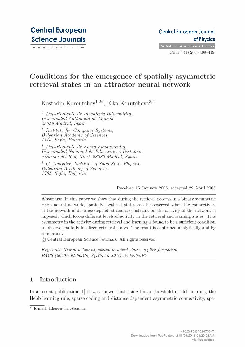
Fig. 1 The components of the first eigenvectors of the connectivity matrix, normalized by thesquare root of their corresponding eigenvalue, in order to eliminate the effect of the size of thenetwork. The first eigenvector has a constant component, the second a sine-like component.N = 6400, c = 320/N, λ0 = 319.8, λ1 = 285.4.
2 Analytical analysis
2.1 Connectivity matrix
For the analytical analysis of the SAS states, we consider the decomposition of the con-
nectivity matrix cij by its eigenvectors a(k)i :
cij =∑
k
λka(k)i a
(k)j ,
∑
i
a(k)i a
(l)i = δkl, (1)
where λk are the corresponding (positive) eigenvalues. The eigenvectors a(k)i are ordered
by their corresponding eigenvalues in decreasing order, e.g.
∀a(k)j , a
(l)j , k > l ⇒ λk ≤ λl. (2)
For convenience we introduce also the parameters bki :
bki ≡ a
(k)i
√
λk/c. (3)
To get some intuition of what the a(k)j look like, we plot in Fig. 1 the first two eigenvectors
a0 and a1.
For a wide variety of connectivities, the first three eigenvectors are approximately the
following:
a(0)k =
√
1/N, a(1)k =
√
2/N cos(2πk/N), a(2)k =
√
2/N sin(2πk/N). (4)
Further, the eigenvalue λ0 is approximately the mean connectivity of the network per
node, that is the mean number of connections per neuron λ0 = cN .
2.2 Hamiltonian
Following the classical analysis of Amit et al. [8], we study the binary Hopfield model [9]
Hint = − 1
cN
∑
ijµ
Siξµi cijξ
µj Sj, (5)
- 10.2478/BF02475647Downloaded from PubFactory at 08/01/2016 08:20:28AM
via free access
K. Koroutchev, E. Korutcheva / Central European Journal of Physics 3(3) 2005 409–419 413
0 0.2 0.4 0.6 0.8 1x=i/N
−0.1
0
0.1
0.2
0.3
m_
(i)
Fig. 2 Typical bump form. The figure shows the running average of the local overlap m(i) = Siξi
vs the position of the neuron (run length 100 and 300). The sparsity of the code is a = 0.2, Ris chosen to supply 0.5 of the unconstrained activity. N = 6400, c = 0.05.
where the matrix cij denotes the connectivity matrix and we have assumed Hebb’s rule
of learning [10].
In order to take into account the finite numbers of overlaps that condense macroscop-
ically, we use Bogolyubov’s method of quasi averages [11]. To this aim we introduce an
external field, conjugate to a final number of patterns {ξνi }, ν = 1, 2, ..., s by adding a
term
Hh = −s∑
ν=1
hν∑
i
ξνi Si (6)
to the Hamiltonian.
Finally, as we mentioned already in the Introduction, in order to impose some asym-
metry in the neural network’s states, we also add the term
Ha = NR
(
1
N
∑
i
Si
)
≈ NRSib0i , (7)
where we used b0i ≈ 1. The equality is exact for an equal degree network. The overline
in eq.(7) means spatial averaging: (.i) = 1N
∑
i(.).
The whole Hamiltonian we are studying now is H = Hint + Hh + Ha:
H = − 1
cN
∑
ijµ
Siξµi cijξ
µj Sj −
s∑
ν=1
hν∑
i
ξνi Si + NRSib
0i . (8)
2.3 RS solution
By using the “replica formalism” [12], for the averaged free energy per neuron we get:
f = limn→0
limN→∞
−1
βnN(〈〈Zn〉〉 − 1), (9)
where 〈〈...〉〉 stands for the average over the pattern distribution P (ξµi ), n is the number
of the replicas, which are later taken to zero, and β is the inverse temperature.
- 10.2478/BF02475647Downloaded from PubFactory at 08/01/2016 08:20:28AM
via free access
414 K. Koroutchev, E. Korutcheva / Central European Journal of Physics 3(3) 2005 409–419
Following [8, 13], the replicated partition function is represented by decoupling the
sites using an expansion of the connectivity matrix cij over its eigenvalues λl, l = 1, ..., M
and eigenvectors ali (eq.1):
〈〈Zn〉〉 = e−βαNn/2c⟨⟨
TrSρ exp[
β
2N
∑
µρl
∑
ij
(ξµi Sρ
i bli)(ξ
µj Sρ
j blj) +
β∑
ν
hν∑
iρ
ξνi Sρ
i − βRN∑
iρ
b0i S
ρi /N
]⟩⟩
, (10)
with α = p/N being the storage capacity.
Following the classical approach of Amit et al.[8] we introduce variables mµρk for each
replica ρ and each eigenvalue and split the sums over the first s “condensed”patterns,
labeled by the letter ν and the remaining (infinite) p − s, over which an average and a
later expansion over their corresponding parameters was done.¶ We have supposed that
only a finite number of mνk are of order one and those are related to the largest eigenvalues
λk.
As a next step, we introduce the order parameters (OP)
qρ,σk = (bk
i )2Sρ
i Sσi ,
where ρ, σ = 1, ..., n label the replica indices. Note the role of the connectivity matrix in
the OP qρ,σk by the introduction of the parameters bk
i .
The introduction of the OP rρ,σk , conjugate to qρ,σ
k , and the use of the replica symmetry
ansatz [12] mνρk = mν
k, qρ,σk = qk for ρ 6= σ and rρ,σ
k = rk for ρ 6= σ, followed by a suitable
linearization of the quadratic in S-terms and the application of the saddle-point method
[8], give the following final form for the free energy per neuron:
f =1
2cα(1 − a2) +
1
2
∑
k
(mk)2 − αβ(1 − a2)
2
∑
k
rkqk +αβ(1 − a2)
2
∑
k
µkrk +
+α
2β
∑
k
[ln(1 − β(1 − a2)µk + β(1 − a2)qk) − (11)
−β(1 − a2)qk(1 − β(1 − a2)µk + β(1 − a2)qk)−1] −
− 1
β
∫
dze−z2
2√2π
ln 2 coshβ
z√
α(1 − a2)∑
l
rlblib
li +
∑
l
mlξibli + Rb0
i
.
In the last expression we have introduced the variables µk = λk/cN and we have used
the fact that the average over a finite number of patterns ξν can be self-averaged [8]. In
our case however the self-averaging is more complicated in order to preserve the spatial
dependence of the retrieved pattern. The detailed analysis will be given in a forthcoming
publication [14].
¶ Without loss of generality we can limit ourself to the case of only one pattern with macroscopic overlap
(ν = 1). The generalization to ν > 1 is straightforward.
- 10.2478/BF02475647Downloaded from PubFactory at 08/01/2016 08:20:28AM
via free access
K. Koroutchev, E. Korutcheva / Central European Journal of Physics 3(3) 2005 409–419 415
The equations for the OP rk, mk and qk are respectively:
rk =qk(1 − a2)
(1 − β(1 − a2)(µk − qk))2 , (12)
mk =∫ dze−
z2
2√2π
ξibki tanh β
z√
α(1 − a2)∑
l
rlblib
li +
∑
l
mlξibli + Rb0
i
(13)
and
qk =∫
dze−z2
2√2π
(bki )
2 tanh2 β
z√
α(1 − a2)∑
l
rlblib
li +
∑
l
mlξibli + Rb0
i
. (14)
At T = 0, keeping Ck ≡ β(µk − qk) finite and limiting the above system only to the
first two coefficients, the above equations read:
m0 =1 − a2
4π
∫ π
−πg(φ)dφ (15)
m1 =√
2µ11 − a2
4π
∫ π
−πg(φ) sinφ dφ (16)
C0 =1
2π
∫ π
−πgc(φ)dφ (17)
C1 =µ1
π
∫ π
−πgc(φ) sin2 φ dφ (18)
rk =µk(1 − a2)
[1 − (1 − a2)Ck]2, (19)
where
g(φ) = erf(x1) + erf(x2) (20)
gc(φ) = [(1 + a)e−(x1)2 + (1 − a)e−(x2)2 ]/[√
πy] (21)
x1 = [(1 − a)(m0 + m1
√
2µ1 sin φ) + R]/y (22)
x2 = [(1 + a)(m0 + m1
√
2µ1 sin φ) − R]/y (23)
y =√
2α(1 − a2)(r0 + 2µ1r1 sin2 φ). (24)
When we assume m1 = m2 = ... = 0, R = 0, we obtain the result of Gardner [13].
When additionally µ1 = 0 we obtain the result of Amit et al. [8]. Of course, in this
approximation no conclusion about the size of the bump can be drawn, because the
characteristic size of the bump is fixed to be the characteristic size of a sine wave, that is
always one half of the size of the network.
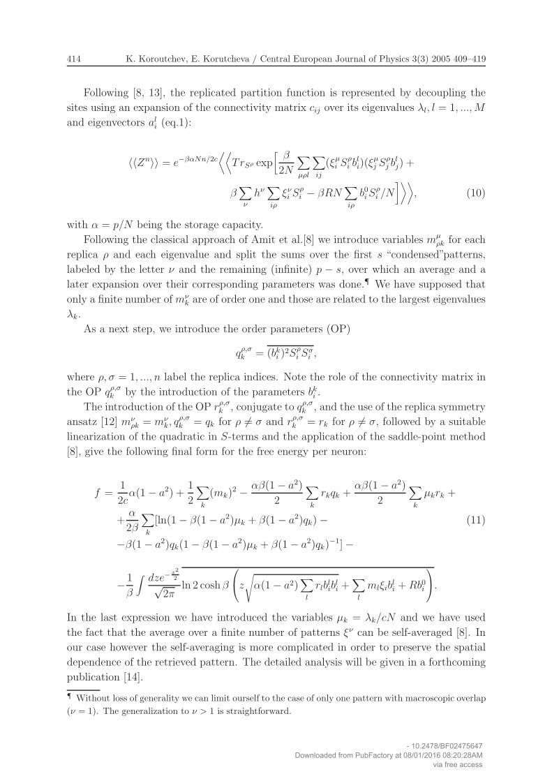
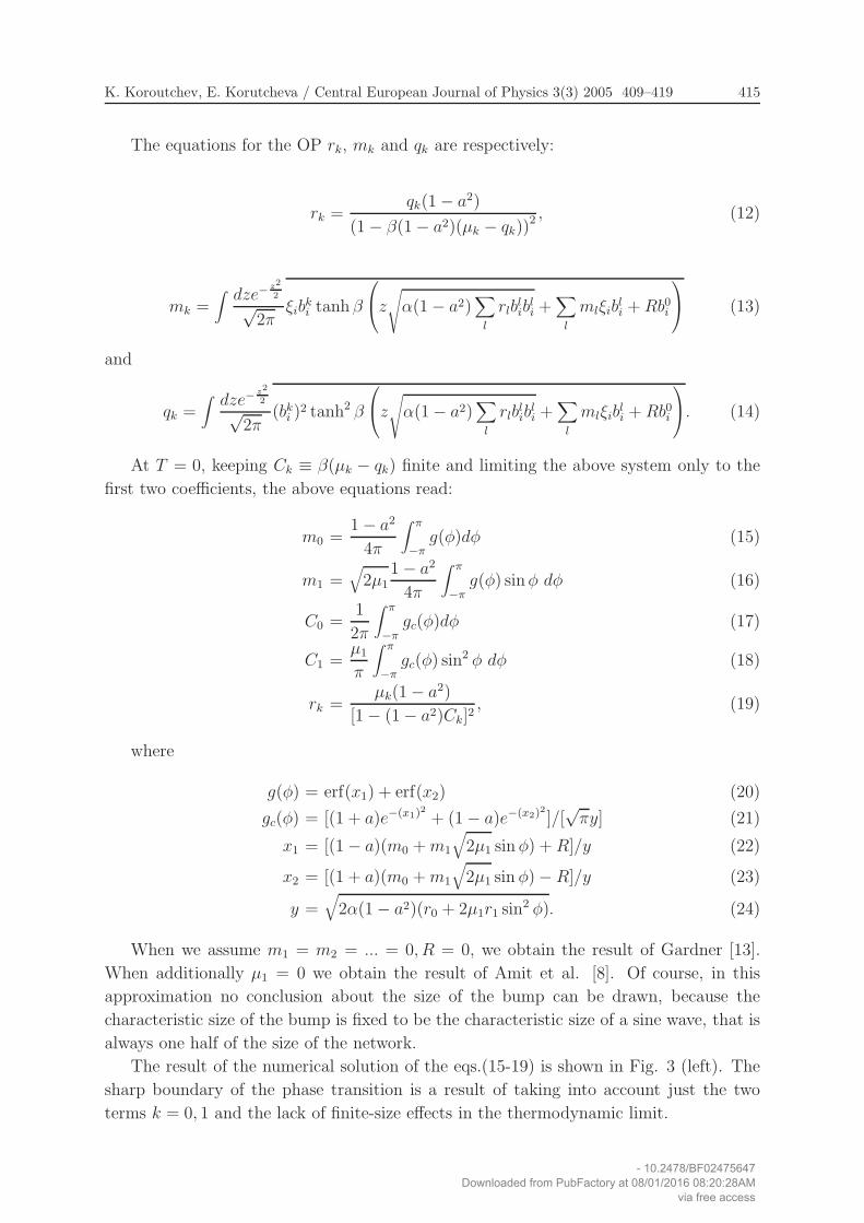
The result of the numerical solution of the eqs.(15-19) is shown in Fig. 3 (left). The
sharp boundary of the phase transition is a result of taking into account just the two
terms k = 0, 1 and the lack of finite-size effects in the thermodynamic limit.
- 10.2478/BF02475647Downloaded from PubFactory at 08/01/2016 08:20:28AM
via free access
416 K. Koroutchev, E. Korutcheva / Central European Journal of Physics 3(3) 2005 409–419
0 0.2 0.4 0.6alpha/c
0
0.1
0.2
0.3
0.4
0.5m
_0,m
_1
m_0m_1
0 0.2 0.4 0.6alpha/c
0
0.1
0.2
0.3
0.4
0.5
m,m
_1
m_1m
Fig. 3 Left – Computation of m0, m1 according to the eqs.(15-19). The sparsity of the code isa = 0.2 and R = 0.57. The sharp boundary is due to the limitation of the equations only tothe first two terms of the OP m, r, C, as well as the lack of finite scale effects. The result of thesimulations is represented on the right side.
3 Simulations
In order to compare the results, we also performed computer simulations. To this aim we
chose the network’s topology to be a circular ring, with a distance measure
|i − j| ≡ min(i − j + N mod N, j − i + N mod N)
and used the same connectivity as in Ref.[1] with a typical connectivity distance σxN :
P (cij = 1) = c
[
1√2πσxN
e−(|i−j|/N)2/2σ2x + p0
]
.
Here the parameter p0 is chosen to normalize the expression in the brackets. When σx is
small enough, then spatial asymmetry is expected.
In order to measure the overlap between the states of the patterns and the neurons
and the effect of the single-bump spatial activity during the simulation, we used the ratio
m1/m0, where
m0 =1
N
∑
k
ξ0kSk
and
m1 =1
N|∑
k
ξ0kSke
2πik/N |.
Because the sine waves appear first, m1/m0 results in a sensitive asymmetric measure
as well, at least compared to the visual inspection of the running averages of the local
overlap m(i) ≡ ξiSi. An example of the local overlap form is given in Fig.2.
Let us note that m1 can be regarded as the power of the first Fourier component and
m0 can be regarded as a zeroth Fourier component, that is the power of the direct-current
component.
The corresponding behavior of the order parameters m0, m1 in the zero-temperature
case, obtained by the simulations, is represented in Fig. 3 (right). Note the good cor-
respondence between the numerical solution of the analytical results and the results ob-
tained by simulation.
- 10.2478/BF02475647Downloaded from PubFactory at 08/01/2016 08:20:28AM
via free access
K. Koroutchev, E. Korutcheva / Central European Journal of Physics 3(3) 2005 409–419 417
0 0.2 0.4 0.6 0.8 1code sparsity a
0
0.2
0.4
0.6
0.8
R
ZSAS
non SASm_0 non zerom_1 zero
0 0.2 0.4 0.6 0.8Code sparsity a
0.4
0.5
0.6
0.7
0.8
R
α=0.1α=0.05α=0.001
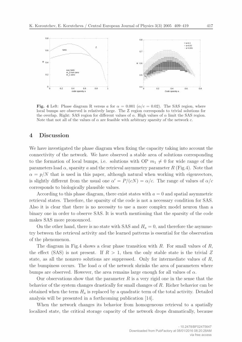
Fig. 4 Left: Phase diagram R versus a for α = 0.001 (α/c = 0.02). The SAS region, wherelocal bumps are observed is relatively large. The Z region corresponds to trivial solutions forthe overlap. Right: SAS region for different values of α. High values of α limit the SAS region.Note that not all of the values of α are feasible with arbitrary sparsity of the network c.
4 Discussion
We have investigated the phase diagram when fixing the capacity taking into account the
connectivity of the network. We have observed a stable area of solutions corresponding
to the formation of local bumps, i.e. solutions with OP m1 6= 0 for wide range of the
parameters load α, sparsity a and the retrieval asymmetry parameter R (Fig.4). Note that
α = p/N that is used in this paper, although natural when working with eigenvectors,
is slightly different from the usual one α′ = P/(cN) = α/c. The range of values of α/c
corresponds to biologically plausible values.
According to this phase diagram, there exist states with a = 0 and spatial asymmetric
retrieval states. Therefore, the sparsity of the code is not a necessary condition for SAS.
Also it is clear that there is no necessity to use a more complex model neuron than a
binary one in order to observe SAS. It is worth mentioning that the sparsity of the code
makes SAS more pronounced.
On the other hand, there is no state with SAS and Ha = 0, and therefore the asymme-
try between the retrieval activity and the learned patterns is essential for the observation
of the phenomenon.
The diagram in Fig.4 shows a clear phase transition with R. For small values of R,
the effect (SAS) is not present. If R > 1, then the only stable state is the trivial Z
state, as all the nonzero solutions are suppressed. Only for intermediate values of R,
the bumpiness occurs. The load α of the network shrinks the area of parameters where
bumps are observed. However, the area remains large enough for all values of α.
Our observations show that the parameter R is a very rigid one in the sense that the
behavior of the system changes drastically for small changes of R. Richer behavior can be
obtained when the term Ha is replaced by a quadratic term of the total activity. Detailed
analysis will be presented in a forthcoming publication [14].
When the network changes its behavior from homogeneous retrieval to a spatially
localized state, the critical storage capacity of the network drops dramatically, because
- 10.2478/BF02475647Downloaded from PubFactory at 08/01/2016 08:20:28AM
via free access
418 K. Koroutchev, E. Korutcheva / Central European Journal of Physics 3(3) 2005 409–419
0.3 0.4 0.5 0.6 0.7R
0
0.02
0.04
0.06
0.08
0.1
Critic
al c
ap
aci
ty α
c
Symmetric
state
SAS
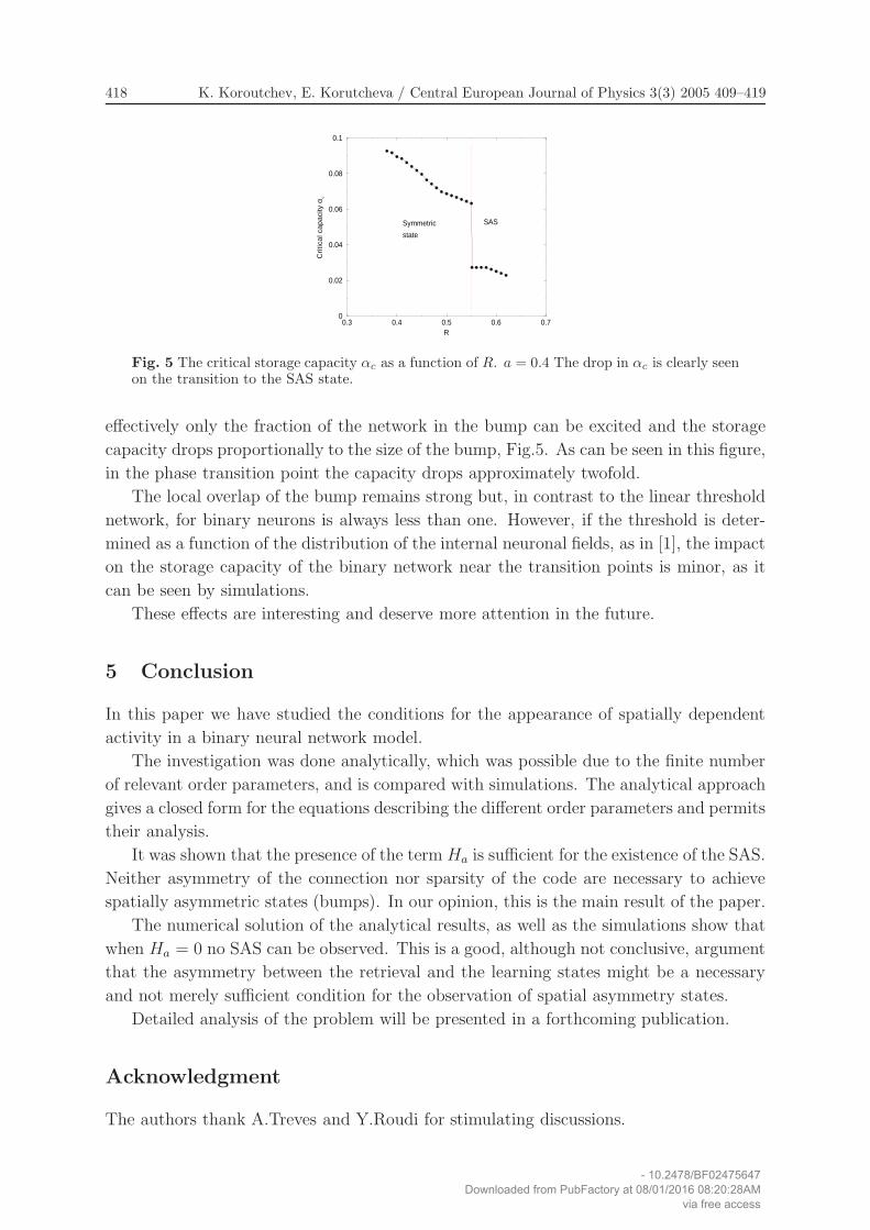
Fig. 5 The critical storage capacity αc as a function of R. a = 0.4 The drop in αc is clearly seenon the transition to the SAS state.
effectively only the fraction of the network in the bump can be excited and the storage
capacity drops proportionally to the size of the bump, Fig.5. As can be seen in this figure,
in the phase transition point the capacity drops approximately twofold.
The local overlap of the bump remains strong but, in contrast to the linear threshold
network, for binary neurons is always less than one. However, if the threshold is deter-
mined as a function of the distribution of the internal neuronal fields, as in [1], the impact
on the storage capacity of the binary network near the transition points is minor, as it
can be seen by simulations.
These effects are interesting and deserve more attention in the future.
5 Conclusion
In this paper we have studied the conditions for the appearance of spatially dependent
activity in a binary neural network model.
The investigation was done analytically, which was possible due to the finite number
of relevant order parameters, and is compared with simulations. The analytical approach
gives a closed form for the equations describing the different order parameters and permits
their analysis.
It was shown that the presence of the term Ha is sufficient for the existence of the SAS.
Neither asymmetry of the connection nor sparsity of the code are necessary to achieve
spatially asymmetric states (bumps). In our opinion, this is the main result of the paper.
The numerical solution of the analytical results, as well as the simulations show that
when Ha = 0 no SAS can be observed. This is a good, although not conclusive, argument
that the asymmetry between the retrieval and the learning states might be a necessary
and not merely sufficient condition for the observation of spatial asymmetry states.
Detailed analysis of the problem will be presented in a forthcoming publication.
Acknowledgment
The authors thank A.Treves and Y.Roudi for stimulating discussions.
- 10.2478/BF02475647Downloaded from PubFactory at 08/01/2016 08:20:28AM
via free access
K. Koroutchev, E. Korutcheva / Central European Journal of Physics 3(3) 2005 409–419 419
This work is financially supported by the Abdus Salam Center for Theoretical Physics,
Trieste, Italy and by Spanish Grants CICyT, TIC 01-572, TIN 2004-07676,
DGI.M.CyT.BFM2001-291-C02-01 and the program ”Promocion de la Investigacion
UNED’02”.
References
[1] Y. Roudi and A. Treves: “An associate network with spatially organized connectivity”,JSTAT, Vol. 1, (2004), P07010.
[2] K. Koroutchev and E. Korutcheva: Spatial asymmetric retrieval states in symmetricHebb network with uniform connectivity, Preprint ICTP, Trieste, Italy, IC/2004/91,(2004), pp. 1–12.
[3] A. Anishchenko, E. Bienenstock and A. Treves: Autoassociative Memory Retrievaland Spontaneous Activity Bumps in Small-World Networks of Integrate-and-FireNeurons, Los Alamos, 2005, http://xxx.lanl.gov/abs/q-bio.NC/0502003.
[4] J. Rubin and A. Bose: “Localized activity in excitatory neuronal networks”, Network:Comput. Neural Syst., Vol. 15, (2004), pp. 133–158.
[5] N. Brunel: “Dynamics and plasticity of stimulus-selective persistent activity incortical network models”, Cereb. Cortex, Vol. 13, (2003), pp. 1151–1161.
[6] J. Hertz, A. Krogh and R.G. Palmer: Introduction to the theory of neuralcomputation, Perseus Publishing Group, Santa Fe, 1991.
[7] M. Tsodyks and M. Feigel’man: “Enhanced storage capacity in neural networks withlow activity level”, Europhys. Lett., Vol. 6, (1988), pp. 101–105.
[8] D. Amit, H. Gutfreund and H. Sompolinsky: “Statistical mechanics of neuralnetworks near saturation”, Ann. Phys., Vol. 173, (1987), pp. 30–67.
[9] J. Hopfield: “Neural networks and physical systems with emergent collectivecomputational abilities”, Proc. Natl. Acad. Sci. USA, Vol. 79, (1982), pp. 2554–2558.
[10] D. Hebb: The Organization of Behavior: A Neurophysiological Theory, Wiley, NewYork, 1949.
[11] N.N. Bogolyubov: Physica(Suppl.), Vol. 26, (1960), pp. 1.
[12] M. Mezard, G. Parisi and M.-A. Virasoro: Spin-glass theory and beyond, WorldScientific, Singapore, 1987.
[13] A. Canning and E. Gardner: “Partially connected models of neural networks”, J.Phys. A: Math. Gen., Vol. 21, (1988), pp. 3275–3284.
[14] K. Koroutchev and E. Korutcheva: in preparation.
- 10.2478/BF02475647Downloaded from PubFactory at 08/01/2016 08:20:28AM
via free access