arX

iv:c

ond-

mat

/050

3626

v2 [

cond

-mat

.sta

t-m

ech]

29

Jun

2005

Conditions for the emergence of spatial

asymmetric retrieval states in attractor neural

network

Kostadin Koroutchev ∗(1) and Elka Korutcheva †(2)

December 9, 2013

(1) Depto. de Ingenierıa InformaticaUniversidad Autonoma de Madrid, 28049 Madrid, Spain

(2) Depto. de Fısica Fundamental,Universidad Nacional de Educacion a Distancia,

c/Senda del Rey, No 9, 28080 Madrid, Spain

Abstract

In this paper we show that during the retrieval process in a bi-nary symmetric Hebb neural network, spatial localized states can beobserved when the connectivity of the network is distance-dependentand constraint on the activity of the network is imposed, which forcesdifferent level of activity in the retrieval and learning states. Thisasymmetry in the activity during the retrieval and learning is foundto be sufficient condition in order to observe spatial localized retrievalstates. The result is confirmed analytically and by simulation. Key-

words: neural networks, spatial localized states, replica formalismPACS: 64.60.Cn, 84.35.+i, 89.75.-k, 89.75.Fb

∗Corresponding author; k.koroutchev@uam.es; Inst. for Computer Systems, BulgarianAcademy of Sciences, 1113, Sofia, Bulgaria

†G.Nadjakov Institute of Solid State Physics, Bulgarian Academy of Sciences, 1784,Sofia, Bulgaria

1

1 Introduction

In a recent publication [1] it was shown that using linear-thresholdmodel neurons, Hebb learning rule, sparse coding and distance-dependentasymmetric connectivity, spatial asymmetric retrieval states (SAS)can be observed. This asymmetric states are characterized by a spatiallocalization of the activity of the neurons, described by the formationof local bumps.

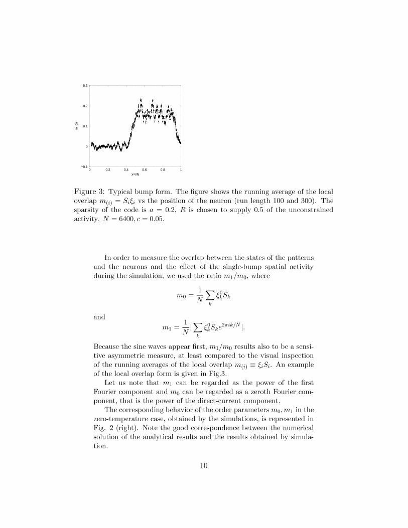
Similar results have been reported in the case of Hebb binary modelfor associative neural network [2]. The observation is intriguing, be-cause all components of the network are intrinsically symmetric withrespect to the positions of the neurons and the retrieved state is clearlyasymmetric. An illustration of SAS in binary network is presented inFig.3.

In parallel to the present investigation, extensive computer simu-lations have been performed in the case of integrate and fire neurons[3], where bump formations were also reported. These results arein agreement with our previous results [2] that networks of binaryneurons do not show bumpy retrieval solutions when the stored andretrieved patterns have the same mean activity.

The biological reason for this phenomenon is based on the transientsynchrony that leads to recruitment of cells into local bumps, followedby desynchronized activity within the group [4],[5].

When the network is sufficiently diluted, say less then 5%, thenthe differences between asymmetric and symmetric connectivity areminimal [6]. For this reason we expect that the impact of the asym-metrical connectivity will be minimal and the asymmetry could notbe considered as necessary condition for the existence of SAS, as it isconfirmed in the present work.

There are several factors that possibly contribute to the SAS inmodel network.

In order to introduce the spatial effects in neural networks(NN),one essentially needs distance measures and topology between theneurons, imposing some distribution on the connections, dependenton that topology and distances. The major factor to observe spatialasymmetric activity is of course the spatially dependent connectiv-ity of the network. Actually this is an essential condition, becausegiven a network with SAS, by applying random permutation to theenumeration of the neurons, one will obviously achieve states withoutSAS. Therefore, the topology of the connections must depend on the

2

distance between the neurons.Due to these arguments, a symmetric and distance-dependent con-

nectivity for all neurons is chosen in this study.We consider an attractor NN model of Hebbian type formed by

N binary neurons {Si}, Si ∈ {−1, 1}, i = 1, ..., N , storing p binarypatterns ξµ

i , µ ∈ {1...p}, and we assume a symmetric connectivitybetween the neurons cij = cji ∈ {0, 1}, cii = 0. cij = 1 means thatneurons i and j are connected. We regard only connectivities in whichthe fluctuations between the individual connectivity are small, e.g.∀i∑

j cij ≈ cN , where c is the mean connectivity.The learned patterns are drawn from the following distribution:

P (ξµi ) =

1 + a

2δ(ξµ

i − 1 + a) +1 − a

2δ(ξµ

i + 1 + a),

where the parameter a is the sparsity of the code. Note that thenotation is a little bit different from the usual one. By changing thevariables η → ξ+a and substituting in the above equation, one obtainsthe usual form for the pattern distribution in the case of sparse code[7].

Further in this article we show that imposing symmetry betweenthe retrieval and the learning states, i.e. equal probability distribu-tions of the patterns and the network activities, no SAS exists. Spatialasymmetry can be observed only when asymmetry between the learn-ing and the retrieval states is imposed.

Actually, by using binary network and symmetrically distributedpatterns, the only asymmetry between the retrieval and the learningstates that can be imposed, independent on the position of the neu-rons, is the total number of the neurons in a given state. Having inmind that there are only two possible states, this condition leads to acondition on the mean activity of the network.

To impose a condition on the mean activity, we add an extra termHa to the Hamiltonian

Ha = NR∑

i

Si/N.

This term actually favors states with lower total activity∑

i Si that isequivalent to decrease the number of active neurons, creating asym-metry between the learning and the retrieval states. If the value ofthe parameter R = 0, the corresponding model has been intensivelystudied since the classical results of Amit et al. [8] for symmetrical

3

code and Tsodyks, Feigel’man [7] for sparse code. These results showthat the sparsities of the learned patterns and the retrieval states arethe same and equal to aN . In the case R 6= 0, the energy of the systemincreases with the number of active neurons (Si = 1) and the termHa tends to limit the number of active neurons below aN . Roughlyspeaking, the parameter R can be interpreted as some kind of chemi-cal potential for the system to force a neuron in a state S = 1. Herewe would like to mention that Roudi and Treves [1] have also statedthat the activity of the linear-threshold network, they study, has tobe constrained in order to have spatially asymmetric states. However,no explicit analysis was presented in order to explain the phenomenonand the condition is not shown to be sufficient one, probably becausethe use of more complicated linear threshold neurons diminishes theimportance of this condition. Here we point out the importance of theconstraint on the network level of activity and show that it is a suffi-cient condition for observation of spatial asymmetric states in binaryHebb neural network.

The goal of this article is to find minimal necessary conditionswhere SAS can be observed. We start with general sparse code andsparse distance-dependent connectivity and using replica symmetryparadigm we find the equations for the order parameters.

Then we study the solutions of these equations using some approx-imations and compare the analytical results with simulation.

The conclusion, drawn in the last part, shows that only the asym-metry between the learning and the retrieval states is sufficient toobserve SAS.

2 Analytical analysis

2.1 Connectivity matrix

For the analytical analysis of the SAS states, we consider the decom-

position of the connectivity matrix cij by its eigenvectors a(k)i :

cij =∑

k

λka(k)i a

(k)j ,

∑

i

a(k)i a

(l)i = δkl, (1)

where λk are the corresponding (positive) eigenvalues. The eigenvec-

tors a(k)i are ordered by its corresponding eigenvalues in decreasing

order, e.g.

∀a(k)j , a

(l)j , k > l ⇒ λk ≤ λl. (2)

4

0 0.2 0.4 0.6 0.8 1x=i/N

−2.00

−1.00

0.00

1.00

2.00

b_

0(x

),b

_1

(x)

bo

b1

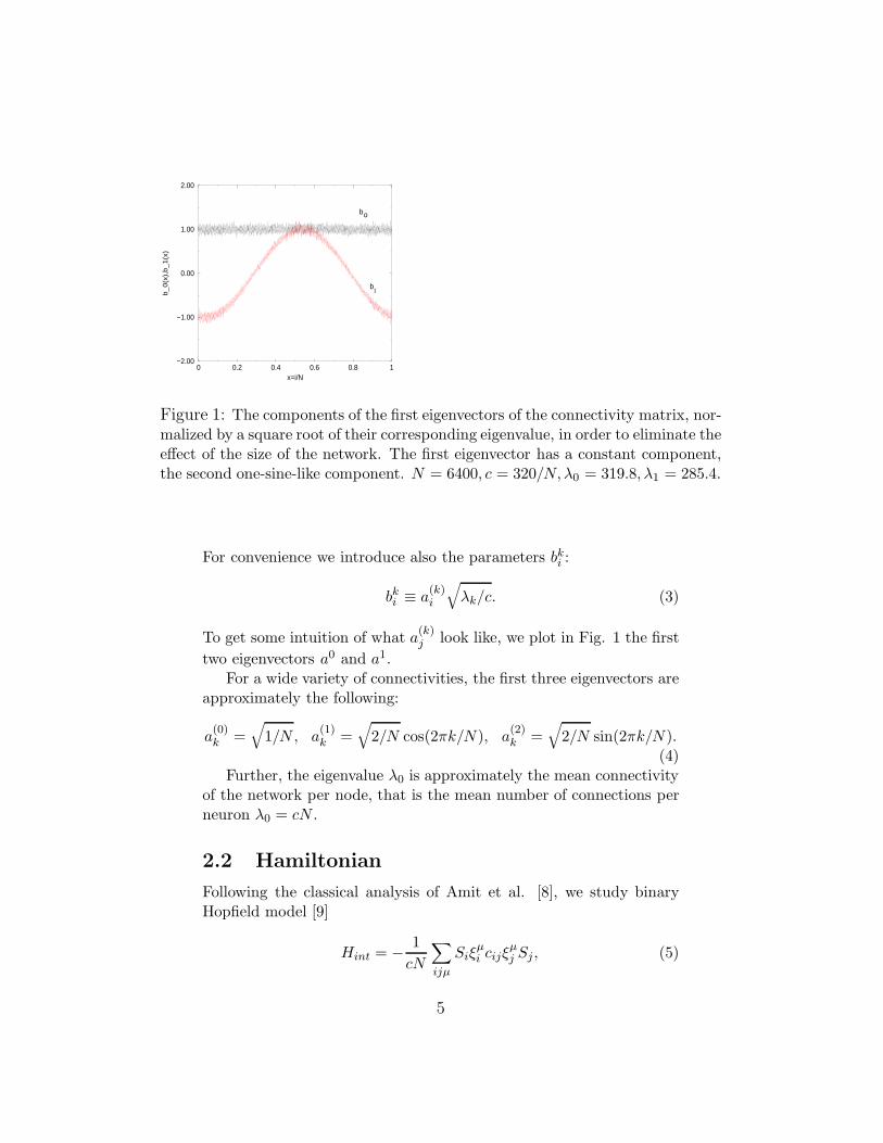
Figure 1: The components of the first eigenvectors of the connectivity matrix, nor-malized by a square root of their corresponding eigenvalue, in order to eliminate theeffect of the size of the network. The first eigenvector has a constant component,the second one-sine-like component. N = 6400, c = 320/N, λ0 = 319.8, λ1 = 285.4.

For convenience we introduce also the parameters bki :

bki ≡ a

(k)i

√

λk/c. (3)

To get some intuition of what a(k)j look like, we plot in Fig. 1 the first

two eigenvectors a0 and a1.For a wide variety of connectivities, the first three eigenvectors are

approximately the following:

a(0)k =

√

1/N, a(1)k =

√

2/N cos(2πk/N), a(2)k =

√

2/N sin(2πk/N).(4)

Further, the eigenvalue λ0 is approximately the mean connectivityof the network per node, that is the mean number of connections perneuron λ0 = cN .

2.2 Hamiltonian

Following the classical analysis of Amit et al. [8], we study binaryHopfield model [9]

Hint = − 1

cN

∑

ijµ

Siξµi cijξ

µj Sj, (5)

5

where the matrix cij denotes the matrix of connectivity and we haveassumed Hebb’s rule of learning [10].

In order to take into account the finite numbers of overlaps thatcondense macroscopically, we use Bogolyubov’s method of quasi aver-ages [11]. To this aim we introduce an external field, conjugate to afinal number of patterns {ξν

i }, ν = 1, 2, ..., s by adding a term

Hh = −s∑

ν=1

hν∑

i

ξνi Si (6)

to the Hamiltonian.Finally, as we already mentioned in the Introduction, in order to

impose some asymmetry in the neural network’s states, we also addthe term

Ha = NR

(

1

N

∑

i

Si

)

≈ NRSib0i , (7)

where we used b0i ≈ 1. The equality is exact for equal degree network.

The over line in eq.(7) means spatial averaging: (.i) = 1N

∑

i(.).The whole Hamiltonian we are studying now is H = Hint+Hh+Ha:

H = − 1

cN

∑

ijµ

Siξµi cijξ

µj Sj −

s∑

ν=1

hν∑

i

ξνi Si + NRSib0

i . (8)

2.3 RS solution

By using the “replica formalism” [12], for the averaged free energy perneuron we get:

f = limn→0

limN→∞

−1

βnN(〈〈Zn〉〉 − 1), (9)

where 〈〈...〉〉 stands for the average over the pattern distribution P (ξµi ),

n is the number of the replicas, which are later taken to zero and β isthe inverse temperature.

Following [8], [13], the replicated partition function is representedby decoupling the sites using an expansion of the connectivity matrixcij over its eigenvalues λl, l = 1, ...,M and eigenvectors al

i (eq.1):

〈〈Zn〉〉 = e−βαNn/2c⟨⟨

TrSρ exp

[

β

2N

∑

µρl

∑

ij

(ξµi Sρ

i bli)(ξ

µj Sρ

j blj) +

β∑

ν

hν∑

iρ

ξνi Sρ

i − βRN∑

iρ

b0i S

ρi /N

]⟩⟩

, (10)

6

with α = p/N being the storage capacity.Following the classical approach of Amit et al.[8] we introduce

variables mµρk for each replica ρ and each eigenvalue and split the

sums over the first s “condensed”patterns, labeled by the letter νand the remaining (infinite) p − s, over which an average and a laterexpansion over their corresponding parameters was done.1 We havesupposed that only a finite number of mν

k are of order one and thoseare related to the largest eigenvalues λk.

As a next step, we introduce the order parameters (OP)

qρ,σk = (bk

i )2Sρ

i Sσi ,

where ρ, σ = 1, ..., n label the replica indexes. Note the role of the con-nectivity matrix on the OP qρ,σ

k by the introduction of the parametersbki .

The introduction of the OP rρ,σk , conjugate to qρ,σ

k , and the useof the replica symmetry ansatz [12] mν

ρk = mνk, q

ρ,σk = qk for ρ 6= σ

and rρ,σk = rk for ρ 6= σ, followed by a suitable linearization of the

quadratic in S-terms and the application of the saddle-point method[8], give the following final form for the free energy per neuron:

f =1

2cα(1 − a2) +

1

2

∑

k

(mk)2 − αβ(1 − a2)

2

∑

k

rkqk +αβ(1 − a2)

2

∑

k

µkrk +

+α

2β

∑

k

[ln(1 − β(1 − a2)µk + β(1 − a2)qk) − (11)

− β(1 − a2)qk(1 − β(1 − a2)µk + β(1 − a2)qk)−1] −

− 1

β

∫

dze−z2

2√2π

ln 2 cosh β

z

√

α(1 − a2)∑

l

rlblib

li +

∑

l

mlξibli + Rb0

i

.

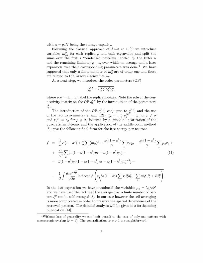
In the last expression we have introduced the variables µk = λk/cNand we have used the fact that the average over a finite number of pat-ters ξν can be self-averaged [8]. In our case however the self-averagingis more complicated in order to preserve the spatial dependence of theretrieved pattern. The detailed analysis will be given in a forthcomingpublication [14].

1Without loss of generality we can limit ourself to the case of only one pattern withmacroscopic overlap (ν = 1). The generalization to ν > 1 is straightforward.

7

The equations for the OP rk, mk and qk are respectively:

rk =qk(1 − a2)

(1 − β(1 − a2)(µk − qk))2 , (12)

mk =

∫

dze−z2

2√2π

ξibki tanh β

z

√

α(1 − a2)∑

l

rlblib

li +

∑

l

mlξibli + Rb0

i

(13)

and

qk =

∫

dze−z2

2√2π

(bki )

2 tanh2 β

z

√

α(1 − a2)∑

l

rlblib

li +

∑

l

mlξibli + Rb0

i

.(14)

At T = 0, keeping Ck ≡ β(µk − qk) finite and limiting the abovesystem only to the first two coefficients, the above equations read:

m0 =1 − a2

4π

∫ π

−πg(φ)dφ (15)

m1 =√

2µ11 − a2

4π

∫ π

−πg(φ) sin φ dφ (16)

C0 =1

2π

∫ π

−πgc(φ)dφ (17)

C1 =µ1

π

∫ π

−πgc(φ) sin2 φ dφ (18)

rk =µk(1 − a2)

[1 − (1 − a2)Ck]2, (19)

where

g(φ) = erf(x1) + erf(x2) (20)

gc(φ) = [(1 + a)e−(x1)2 + (1 − a)e−(x2)2 ]/[√

πy] (21)

x1 = [(1 − a)(m0 + m1

√

2µ1 sin φ) + R]/y (22)

x2 = [(1 + a)(m0 + m1

√

2µ1 sin φ) − R]/y (23)

y =√

2α(1 − a2)(r0 + 2µ1r1 sin2 φ). (24)

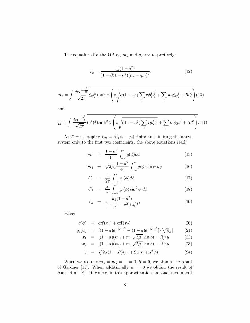
When we assume m1 = m2 = ... = 0, R = 0, we obtain the resultof Gardner [13]. When additionally µ1 = 0 we obtain the result ofAmit et al. [8]. Of course, in this approximation no conclusion about

8

0 0.2 0.4 0.6alpha/c

0

0.1

0.2

0.3

0.4

0.5

m_0

,m_1

m_0m_1

0 0.2 0.4 0.6alpha/c

0

0.1

0.2

0.3

0.4

0.5

m,m

_1

m_1m

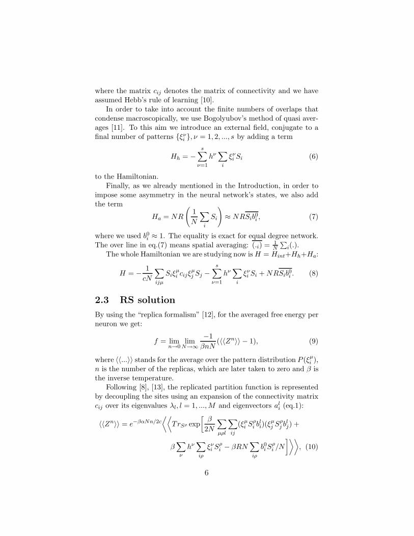
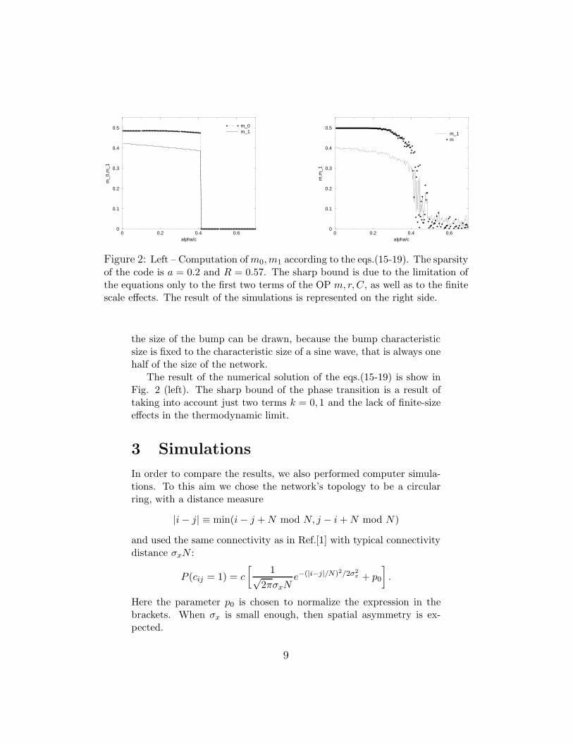
Figure 2: Left – Computation of m0,m1 according to the eqs.(15-19). The sparsityof the code is a = 0.2 and R = 0.57. The sharp bound is due to the limitation ofthe equations only to the first two terms of the OP m, r,C, as well as to the finitescale effects. The result of the simulations is represented on the right side.

the size of the bump can be drawn, because the bump characteristicsize is fixed to the characteristic size of a sine wave, that is always onehalf of the size of the network.

The result of the numerical solution of the eqs.(15-19) is show inFig. 2 (left). The sharp bound of the phase transition is a result oftaking into account just two terms k = 0, 1 and the lack of finite-sizeeffects in the thermodynamic limit.

3 Simulations

In order to compare the results, we also performed computer simula-tions. To this aim we chose the network’s topology to be a circularring, with a distance measure

|i − j| ≡ min(i − j + N mod N, j − i + N mod N)

and used the same connectivity as in Ref.[1] with typical connectivitydistance σxN :

P (cij = 1) = c

[

1√2πσxN

e−(|i−j|/N)2/2σ2x + p0

]

.

Here the parameter p0 is chosen to normalize the expression in thebrackets. When σx is small enough, then spatial asymmetry is ex-pected.

9

0 0.2 0.4 0.6 0.8 1x=i/N

−0.1

0

0.1

0.2

0.3

m_

(i)

Figure 3: Typical bump form. The figure shows the running average of the localoverlap m(i) = Siξi vs the position of the neuron (run length 100 and 300). Thesparsity of the code is a = 0.2, R is chosen to supply 0.5 of the unconstrainedactivity. N = 6400, c = 0.05.

In order to measure the overlap between the states of the patternsand the neurons and the effect of the single-bump spatial activityduring the simulation, we used the ratio m1/m0, where

m0 =1

N

∑

k

ξ0kSk

and

m1 =1

N|∑

k

ξ0kSke

2πik/N |.

Because the sine waves appear first, m1/m0 results also to be a sensi-tive asymmetric measure, at least compared to the visual inspectionof the running averages of the local overlap m(i) ≡ ξiSi. An exampleof the local overlap form is given in Fig.3.

Let us note that m1 can be regarded as the power of the firstFourier component and m0 can be regarded as a zeroth Fourier com-ponent, that is the power of the direct-current component.

The corresponding behavior of the order parameters m0,m1 in thezero-temperature case, obtained by the simulations, is represented inFig. 2 (right). Note the good correspondence between the numericalsolution of the analytical results and the results obtained by simula-tion.

10

0 0.2 0.4 0.6 0.8 1code sparsity a

0

0.2

0.4

0.6

0.8

R

ZSAS

non SASm_0 non zerom_1 zero

0 0.2 0.4 0.6 0.8Code sparsity a

0.4

0.5

0.6

0.7

0.8

R

α=0.1α=0.05α=0.001

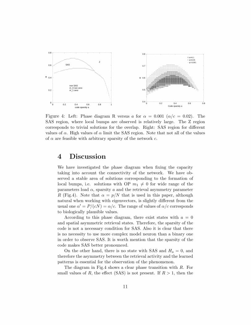
Figure 4: Left: Phase diagram R versus a for α = 0.001 (α/c = 0.02). TheSAS region, where local bumps are observed is relatively large. The Z regioncorresponds to trivial solutions for the overlap. Right: SAS region for differentvalues of α. High values of α limit the SAS region. Note that not all of the valuesof α are feasible with arbitrary sparsity of the network c.

4 Discussion

We have investigated the phase diagram when fixing the capacitytaking into account the connectivity of the network. We have ob-served a stable area of solutions corresponding to the formation oflocal bumps, i.e. solutions with OP m1 6= 0 for wide range of theparameters load α, sparsity a and the retrieval asymmetry parameterR (Fig.4). Note that α = p/N that is used in this paper, althoughnatural when working with eigenvectors, is slightly different from theusual one α′ = P/(cN) = α/c. The range of values of α/c correspondsto biologically plausible values.

According to this phase diagram, there exist states with a = 0and spatial asymmetric retrieval states. Therefore, the sparsity of thecode is not a necessary condition for SAS. Also it is clear that thereis no necessity to use more complex model neuron than a binary onein order to observe SAS. It is worth mention that the sparsity of thecode makes SAS better pronounced.

On the other hand, there is no state with SAS and Ha = 0, andtherefore the asymmetry between the retrieval activity and the learnedpatterns is essential for the observation of the phenomenon.

The diagram in Fig.4 shows a clear phase transition with R. Forsmall values of R, the effect (SAS) is not present. If R > 1, then the

11

0.3 0.4 0.5 0.6 0.7R

0

0.02

0.04

0.06

0.08

0.1

Critic

al c

ap

aci

ty α

c

Symmetric

state

SAS

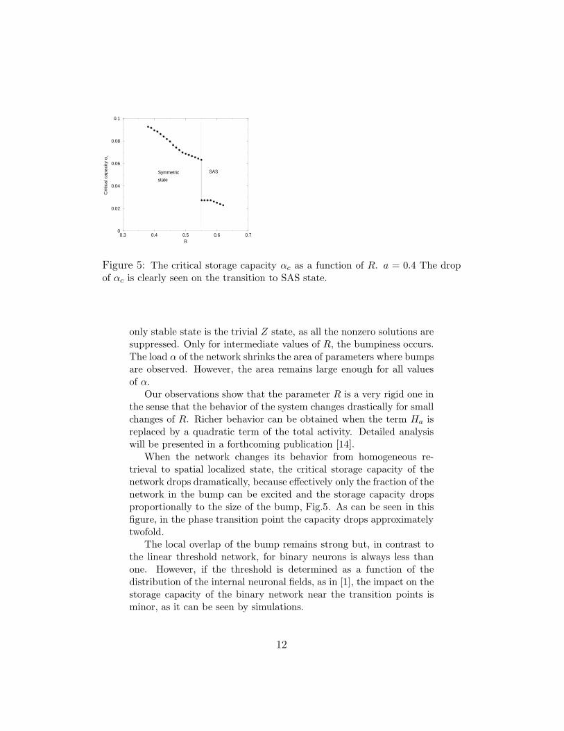
Figure 5: The critical storage capacity αc as a function of R. a = 0.4 The dropof αc is clearly seen on the transition to SAS state.

only stable state is the trivial Z state, as all the nonzero solutions aresuppressed. Only for intermediate values of R, the bumpiness occurs.The load α of the network shrinks the area of parameters where bumpsare observed. However, the area remains large enough for all valuesof α.

Our observations show that the parameter R is a very rigid one inthe sense that the behavior of the system changes drastically for smallchanges of R. Richer behavior can be obtained when the term Ha isreplaced by a quadratic term of the total activity. Detailed analysiswill be presented in a forthcoming publication [14].

When the network changes its behavior from homogeneous re-trieval to spatial localized state, the critical storage capacity of thenetwork drops dramatically, because effectively only the fraction of thenetwork in the bump can be excited and the storage capacity dropsproportionally to the size of the bump, Fig.5. As can be seen in thisfigure, in the phase transition point the capacity drops approximatelytwofold.

The local overlap of the bump remains strong but, in contrast tothe linear threshold network, for binary neurons is always less thanone. However, if the threshold is determined as a function of thedistribution of the internal neuronal fields, as in [1], the impact on thestorage capacity of the binary network near the transition points isminor, as it can be seen by simulations.

12

These effects are interesting and deserves more attention in thefuture.

5 Conclusion

In this paper we have studied the conditions for the appearance ofspatial dependent activity in a binary neural network model.

The analysis was done analytically, which was possible due to thefinite number of relevant order parameters, and is compared with sim-ulations. The analytical approach gives a closed form for the equationsdescribing the different order parameters and permits their analysis.

It was shown that the presence of the term Ha is sufficient forthe existence of the SAS. Nor asymmetry of the connection, neithersparsity of the code are necessary to achieve spatial asymmetric states(bumps). In our opinion, this is the main result of the paper.

The numerical solution of the analytical results, as well as thesimulations show that when Ha = 0 no SAS can be observed. This is agood, although not conclusive argument, that the asymmetry betweenthe retrieval and the learning states might be a necessary and not onlysufficient condition for the observation of spatial asymmetry states.

Detailed analysis of the problem will be presented in a forthcomingpublication.

Acknowledgments

The authors thank A.Treves and Y.Roudi for stimulating discussions.This work is financial supported by the Abdus Salam Center for

Theoretical Physics, Trieste, Italy and by Spanish Grants CICyT, TIC01-572, DGI.M.CyT.BFM2001-291-C02-01 and the program “Promocionde la Investigacion UNED’02”.

References

[1] Y.Roudi and A.Treves, “An associate network with spatially or-ganized connectivity” , JSTAT (2004) P07010, pp. 1-25.

13

[2] K.Koroutchev and E.Korutcheva, “Spatial asymmetric retrievalstates in symmetric Hebb network with uniform connectivity”,Preprint ICTP, Trieste, Italy, IC/2004/91, (2004), pp. 1-12.

[3] A.Anishchenko, E.Bienenstock and A.Treves, AutoassociativeMemory Retrieval and Spontaneous Activity Bumps in Small-World Networks of Integrate-and-Fire Neurons, Los Alamos,2005, http://xxx.lanl.gov/abs/q-bio.NC/0502003.

[4] J.Rubin and A.Bose, “Localized activity in excitatory neuronalnetworks”, Network: Comput.Neural Syst., vol.15,(2004), pp.133-158.

[5] N.Brunel, “Dynamics and plasticity of stimulus-selective per-sistent activity in cortical network models”, Cereb.Cortex,vol.13,(2003),pp.1151-1161.

[6] J. Hertz, A. Krogh and R. G. Palmer, Introduction to the theoryof neural computation, Perseus Publishing Group, Santa Fe, 1991.

[7] M.Tsodyks and M.Feigel’man, “Enhanced storage capacityin neural networks with low activity level”, Europhys.Lett.,vol.6,(1988), pp. 101-105.

[8] D.Amit, H.Gutfreund and H.Sompolinsky, “Statistical me-chanics of neural networks near saturation”,Ann.Phys.,vol.173,(1987),pp.30-67.

[9] J.Hopfield, “Neural networks and physical systems with emer-gent collective computational abilities”, Proc.Natl.Acad.Sci.USA,vol.79,(1982), pp. 2554-2558.

[10] D.Hebb, The Organization of Behavior: A NeurophysiologicalTheory, Wiley, New York, 1949.

[11] N.N.Bogolyubov, Physica(Suppl.), vol.26,(1960), S1.

[12] M.Mezard, G.Parisi and M.-A.Virasoro, Spin-glass theory and be-yond, World Scientific, Singapore, 1987.

[13] A.Canning and E.Gardner, “Partially connected models of neuralnetworks”, J.Phys.A:Math.Gen., vol.21,(1988),pp.3275-3284.

[14] K.Koroutchev and E.Korutcheva, in preparation.

14