The Consumption-Wealth Ratio Under

Asymmetric Adjustment∗

Vasco J. Gabriel†

Department of Economics, University of Surrey, UK and NIPE-UM

Fernando Alexandre

Department of Economics and NIPE, University of Minho, Portugal

Pedro Bacao

GEMF and Faculty of Economics of the University of Coimbra, Portugal

23rd April 2007

Abstract

This paper argues that nonlinear adjustment may provide a better explanation

of fluctuations in the consumption-wealth ratio. The nonlinearity is captured by

a Markov-switching vector error-correction model that allows the dynamics of the

relationship to differ across regimes. Estimation of the system suggests that these

states are related to the behaviour of financial markets. In fact, estimation of the

system suggests that short-term deviations in the consumption-wealth ratio will forecast

either asset returns or consumption growth: the first when changes in wealth are

transitory; the second when changes in wealth are permanent. Our approach uncovers

a richer and more complex dynamics in the consumption-wealth ratio than previous

results in the literature, whilst being in accordance with theoretical predictions of

standard models of consumption under uncertainty.JEL Classification: C32; C5; E21; E44; G10

Keywords: Consumption; Financial markets; Uncertainty; Forecast; Markov switching

∗The authors acknowledge financial support provided by the Portuguese Foundation for Science and

Technology under research grant POCI/EGE/56054/2004 (partially funded by FEDER). We are grateful

to Maximo Camacho for help with his GAUSS procedure. We are also grateful for the comments received

from participants at University of Surrey and University of Minho seminars, and at the International

Atlantic Economic Society 2005 conference, held in New York.†Corresponding author. Address: Department of Economics, University of Surrey, Guildford, Surrey,

GU2 7XH, UK. Email: v.gabriel@surrey.ac.uk. Tel: + 44 1483 682769. Fax: + 44 1483 689548.

1

1 Introduction

There has been a renewed interest in the literature concerning the linkages between asset

wealth and consumption. Indeed, the preceding decade has witnessed remarkable changes

in households’ wealth, particularly due to stock market valuations, which may have had

implications for the pattern of consumer spending. On the other hand, movements

in aggregate macroeconomic relationships, such as the consumption-wealth ratio, may

provide some guidance on the future performance of asset markets. (Lettau and Ludvigson

2001) and (Lettau and Ludvigson 2004) (L&L henceforth), as well as (Ludvigson and

Steindel 1999) and (Poterba 2000), for example, provide recent accounts of the subject.

L&L start from a fairly standard model of consumer behaviour involving consumption,

asset wealth and labour income, which implies that fluctuations in the consumption

wealth-ratio forecast changes in one of these variables. In order to disentangle this

question, these authors estimate a vector error-correction model (VECM) and conclude

that adjustment from shocks distorting the long-run equilibrium takes place mainly through

asset returns. This, in turn, means that deviations from the common trend embody agents’

expectations of future returns on the market portfolio and, therefore, are a useful predictor

of stock and excess returns.

However, given the nature of the variables, it is likely that these adjustments occur in

different ways, depending on the state of economy and, in particular, on the phase of the

stock market. Indeed, asset wealth displays a more volatile behaviour than consumption

or labour income, a feature that is clearly linked with the state of asset markets. Several

papers document the existence of different regimes in financial markets; see (Cecchetti,

Lam, and Mark 1990), (Bonomo and Garcia 1994) and (Driffill and Sola 1998), for example.

Therefore, in this paper, we argue that regime switching may provide a better explanation

for fluctuations in the consumption-wealth ratio. We explicitly allow for different states, by

postulating that the dynamics of the equilibrium errors follow a Markov-switching process.

This, in turn, leads to a Markov-switching VECM (MS-VECM) representation of the

trivariate relationship, which we use to investigate the possibility of nonlinear adjustment

in the consumption-wealth ratio.

Estimation of this MS-VECM suggests that the mechanism through which deviations

2

from the long-run relationship are eliminated depends on the state of the economy. Thus,

we find a regime whereby wealth does most of the error-correction in the system, coinciding

with periods of “bullish” markets. However, we also identify a more “tranquil” state,

where it is consumption growth that drives the system back to long-run equilibrium.

Therefore, and unlike L&L, our findings suggest that short-term deviations in the trivariate

relationship (consumption, labour income and non-human wealth) will forecast either asset

returns or consumption growth, depending on the state of the economy.

These results seem to provide a more accurate description of the dynamics of the

consumption-wealth ratio than the standard, linear specification, while being consistent

with the theoretical framework employed by L&L. Our results also help to explain why

other researchers — (Davis and Palumbo 2001), or (Mehra 2001), among others — found

consumption to adjust sluggishly to shocks in income and wealth. In fact, single-equation

error-correction models with consumption growth as the dependent variable will partly

detect the adjustments in consumption that occur in the regime where markets are less

volatile, although the main driving force of the system is the behaviour of asset wealth.

A Markov-switching type of asymmetric adjustment in cointegrated systems has been

suggested by (Psaradakis, Sola, and Spagnolo 2004) and (Camacho 2005). These papers

form the basis of the methodology employed in this study. (Paap and van Dijk 2003)

employ a similar method, using a Bayesian approach to estimate possible Markov trends

in the consumption-income relationship. However, they do not include asset wealth in their

model and therefore they do not capture the dynamic features present in the cointegrated

system studied by L&L.

Our paper is organised as follows. The next section briefly reviews the model employed

by L&L, reassesses their results and argues that the characteristics of the data calls for

the estimation of a nonlinear specification. Section 3 presents a possible account of the

switching nature of consumption-wealth adjustment. In section 4 we discuss econometric

tests for nonlinear adjustment and apply them to the L&L data. System estimation is

carried out in section 5. Section 6 summarises and concludes.

3

2 Background discussion

In this section, we briefly review the model employed by L&L and point out why their

results (and economic theory) suggest that a nonlinear framework may offer a better

characterisation of the evolution of consumption and the components of wealth. We begin

by considering a standard household budget constraint. Define Wt as the beginning of

period aggregate wealth in period t, with a asset wealth component, At, and a human

capital component, Ht. By letting Ct denote aggregate consumption in period t and Rw,t+1

denote the net return on Wt, a simple wealth accumulation equation is given by

Wt+1 = (1 + Rw,t+1)(Wt − Ct). (1)

Based on this equation, (Campbell and Mankiw 1989) derive an expression for the

consumption-wealth ratio in logs. They take a first-order Taylor expansion of the equation,

solve the difference equation forward and take expectations, resulting in

ct − wt = Et

∞∑

i=1

ρiw(rw,t+i −∆ct+i), (2)

where r = log(1 + R), ρw = (W − C)/W is the steady-state ratio of new investment to

total wealth, and lower case letters denote variables in logs.

Despite the fact that Ht is not observable, L&L show that an empirically valid approximation

may be obtained by using labour income, Yt, as a proxy for human capital, Ht, resulting

in the following log consumption-wealth ratio

ct − αaat − αyyt ≈ Et

∞∑

i=1

ρiw((1− v)rat+i −∆ct+i + v∆yt+1+i), (3)

where (1− v) and v represent the steady-state shares of the wealth components at and yt,

respectively, and rat+i denotes the net returns on asset wealth. The L&L papers provide

a detailed discussion of the assumptions employed in the approximation. L&L then show

that ct, at and yt share a common trend, with cointegration vector (1,−αa,−αy) and

cointegration residual ct − αaat − αyyt (cayt in brief). Importantly for our argument,

equation (3) implies that fluctuations in the consumption-wealth ratio will reflect future

changes in asset wealth, consumption or labour income.

L&L proceed with their analysis by testing for the number of cointegration vectors,

which they conclude to be only one. The cointegrating vector is estimated by the Dynamic

4

OLS method of (Stock and Watson 1993) as (1,−0.3,−0.6), but the results appear to be

robust with respect to the estimation method; therefore, our analysis will also employ

this estimate. Secondly, L&L estimate a vector error-correction model (VECM) of the

trivariate system, with the estimated cointegration vector imposed as the long-run attractor.

The authors conclude that when a shock occurs, it is asset wealth that does most of the

subsequent adjustment in order to restore the common trend.

However, a closer look at the results of L&L seems to suggest that the dynamic

structure of the system may be further explored. 1 Take, for instance, the estimated

equilibrium error cayt = ct − 0.3at − 0.6yt depicted in Figure 1. It suggests that the

adjustment dynamics follows the cyclical patterns of asset markets, as recognised by

(Lettau and Ludvigson 2004, p. 291). This is natural, given the presence of at in the

long-run relationship. The “bull markets” of the late 1960s and late 1990s, for example,

are clearly identified as periods where wealth seems to be above its equilibrium path.

Notice also that these cycles are irregular, thus implying that equilibrium is most likely

being restored in an asymmetric fashion.

On the other hand, a more detailed inspection of the results of the linear VECM reveals

some potential specification problems. Table 1 reports results of maximum likelihood

estimation of a first-order VECM, as well as of standard single and multi-equation specification

tests. The order of the VECM was chosen to be 1 by all tests and information criteria

employed. In addition, we report heteroskedastic and autocorrelation consistent (HAC)

asymptotic standard errors, computed with the plug-in procedure and the Quadratic

Spectral kernel, as suggested by (Andrews and Monahan 1992). This table is comparable

to Table 1 in (Lettau and Ludvigson 2004). Analysing the results of the specification tests,

it is clear that the estimated model appears to suffer from problems on all counts. Looking

at individual equations, the LM test for autocorrelation up to 5 lags points to problems

in the consumption equation, while heteroskedasticity (as revealed by a White test) and1In what follows, we resort to an updated version of the dataset used in (Lettau and Ludvigson 2004).

A detailed description of the data can be found in their Appendix A. The data itself is available from

Ludvigsons’s webpage (http://www.econ.nyu.edu/user/ludvigsons/). The results do not change if the

actual data in (Lettau and Ludvigson 2004) is used instead. The dataset comprises quarterly data on

aggregate consumption, asset wealth and labour income, spanning from the fourth quarter of 1951 to the

third quarter of 2003.

5

ARCH (LM statistic) mainly affects the wealth equation. Moreover, a Jarque-Bera test for

normality indicates that the assumption of normal errors is violated. If the whole system

is considered, the conclusions appear to be the same. Therefore, the use of HAC standard

errors seems justified. Notice that, although the conclusions of L&L are not altered, the

t-ratio (2.228) of the adjustment coefficient associated with wealth growth is significantly

lower.

A possible explanation for these results lies in the stochastic properties of the variables

in the system. Take, for example, consumption and wealth. It is clear from Figure 2, which

represents the levels and growth rates of these variables, that a linear specification is hardly

compatible with the exhibited dynamics. In particular, asset wealth displays not only a

much more volatile path than consumption, but also the volatility seems to be changing

over time. This fact is acknowledged by (Lettau and Ludvigson 2004, p. 277), but it is

not explicitly accounted for. Indeed, a simple mean-variance switching representation for

the first difference of log asset wealth illustrates this point. Figure 3 plots the estimated

variance against asset wealth growth, revealing the time-varying nature of asset wealth

growth volatility. We discuss possible ways to account for this feature in the next section.

3 Regime switching and consumption

The short-run variance of asset wealth is essentially driven by asset-price volatility. Financial

markets are known to experience “changes of mood” , i.e., regime switching, probably

derived from regime switching in dividends — see, e.g., (Driffill and Sola 1998). This fact

has implications for consumption behaviour. For example, (Guidolin and Timmermann

2005) argue that the optimal consumption behaviour of an investor depends on the

nature of the regime switches of asset returns. This implication is easily derived from

simple, standard models of consumption behaviour under uncertainty, such as the example

presented next.

Assume that a consumer lives for two periods. In the first period there is a shock (ε1)

to the consumer’s wealth as a result of an increase in asset prices. However, the consumer

is unsure whether the shock is permanent or temporary, i.e., whether there will be an

offsetting shock in the second period (ε2). The problem of the consumer is to maximise

6

expected life-time utility as of the first period:

maxE1 [u (C1) + u (C2)] , (4)

subject to the budget constraints:

C1 + A1 = L1 + A0 + ε1 (5)

and

C2,s = L2 + A1 + ε2,s, s = 1, 2, (6)

where C1 is consumption in the first period, C2,s is consumption in the second period

when the second-period shock takes the value ε2,s, Ai is asset wealth at the end of period i

(excluding the shock) and Li is labour income in period i. The model incorporates several

simplifications to allow the results to come through as clearly as possible; for instance, there

is no time discounting and inflation is zero (all variables are in real terms). The consumer

has to choose consumption and asset holdings in the first period, and consumption in the

second period contingent on the second-period shock. The life-time budget constraint is:

C1 + C2,s = A0 + L1 + L2 + ε1 + ε2,s, s = 1, 2. (7)

If the shock were temporary, call it state 1, then ε2 = ε2,1 = −ε1 and therefore lifetime

wealth would be what it would have been in the absence of any shock: A0 + L1 + L2.

If the shock to wealth were permanent, call it state 2, then ε2 = ε2,2 = 0. Given the

second-period values, equation (6) implies C2,2 = C2,1 + ε1.

Letting ui denote the marginal utility of consumption in period i (as usual, assumed to

be a decreasing function), the first-order conditions of the maximisation problem imply:

u1 = E1 (u2) (8)

Let P be the probability that the consumer assigns to the occurrence of state 2 and

let u2,i denote the marginal utility of consumption in the second period in state i. The

previous equation can be written as:

u1 = (1− P ) u2,1 + Pu2,2 (9)

If the consumer correctly believes that the shock is permanent (ε2 = 0, P = 1), then

equation (9) becomes u1 = u2,2 and therefore C1 = C2,2, i.e., consumption in the first

7

period will adjust fully to the new “long-run” value. In case the shock is wrongly believed

to be permanent (ε2 = −ε1, P = 1), the consumer will first increase consumption and

later, after the mistake is known, will decrease it. If the shock were correctly believed to

be temporary (ε2 = −ε1, P = 0), then the consumer would not react to it. Instead, asset

wealth would temporarily increase in the first period and then return to normal in the

second period, i.e., wealth would be doing all of the adjustment. In the case where the

consumer wrongly believes the shock to be temporary (ε2 = 0, P = 0), the consumer will

let wealth adjust in the first period. In the second period, after realising the true nature

of the shock, the consumer will adjust consumption.

The message of this simple model is that the adjustment of consumption and wealth to

shocks, and their relation with the consumption-wealth ratio, will depend on the nature of

those shocks and on how they are perceived by the consumer. For instance, if an increase in

wealth is temporary, and seen as such, the consumption-wealth ratio will initially decrease

as a result of that increase in wealth. In this case, this change in the consumption-wealth

ratio will signal a future decline in wealth, which will restore the long-run equilibrium,

after the temporary nature of the shock reveals itself. On the contrary, if the shock

is permanent, but viewed as temporary, then the consumption-wealth ratio will initially

decrease (as a result of the increase in wealth), but subsequently it is consumption that will

increase, i.e., in this case the movement in the consumption-wealth ratio would forecast

the change in consumption.

If the nature of the shocks varies over time (probably accompanying changes in the

state of financial markets), then the implications of the foregoing analysis are clear: the

adjustment of consumption and wealth to shocks should be modelled with a nonlinear

specification to accommodate changes in the dynamics, such as the ones described above.

In the next section, we consider a formal approach to testing for nonlinear adjustment.

We also introduce a multivariate Markov-switching representation of the trivariate relationship

studied by L&L. This representation will be estimated and tested in section 5.

8

4 Testing for asymmetric adjustment

Following the discussion above, in this section we investigate the possibility of asymmetric

adjustment in the consumption-wealth linkage. There is a difficulty in casting the testing

problem in the usual framework (null of no cointegration vs. null of nonlinear cointegration),

as some parameters will not be identified under the null. We follow the multi-step approach

suggested in (Psaradakis, Sola, and Spagnolo 2004) to detect nonlinear error-correction.

As a first step, conventional procedures to establish the “global” properties of the series

(such as unit root and cointegration tests) remain valid, as long as regularity conditions are

obeyed (even though the deviations from the long-run equilibrium (zt) may be nonlinear).

Once cointegration between the variables is discovered, a second step follows, focusing

on the potential nonlinear “local” characteristics of the system, by looking at either the

equilibrium error (in our case cayt = ct − 0.3at − 0.6yt), or the associated error-correction

model for signs of nonlinear adjustment. This task may be carried out by using a range

of tests that include parameter instability tests (for example, those of (Hansen 1992b)

or (Andrews and Ploberger 1994)), general tests for neglected nonlinearity (e.g., RESET,

White, Neural Networks) or nonlinearity tests designed to test linear adjustment against

nonlinear error-correction alternatives, such as Markov switching ((Hansen 1992a)) and

threshold adjustment ((Hansen 1997) and (Hansen 1999)). Moreover, and as suggested by

(Psaradakis, Sola, and Spagnolo 2004), we may also resort to conventional model selection

criteria such as the AIC (or BIC and Hannan-Quinn criteria), which was found to perform

well in these circumstances.

If the analysis of the “local” features of the data points to nonlinearity, then a third

step ensues, in which one should fit a MS model, either to zt or to the error-correction

representation. However, in the case considered here, the results in L&L indicate that

wealth does most of the adjustment towards equilibrium, meaning that a single-equation

ECM with consumption as the dependent variable would be misspecified. Thus, one needs

to analyse the whole system, which implies that a Markov-switching vector error-correction

model should be employed instead.

(Camacho 2005) shows that if the equilibrium errors of a cointegrated system for the

9

m×m vector xt follow a MS-(V)AR,

zt = cst + Ast(L)zt−1 + θstεt (10)

then there is a corresponding MS-VECM representation

∆xt = µst+ Γstzt−1 + Πst(L)∆xt−1 + σstut (11)

where Πi’s are m×m coefficient matrices and Γst is a regime-dependent long-run impact

matrix. Indeed, the nonlinear dynamics of the equilibrium errors zt may lead to a switching

adjustment matrix Γ and to short-run dynamics of the endogenous variables (given by Π)

that vary across regimes. Several possibilities may arise, including one where cointegration

switches on and off, for example. The system may be estimated by a multi-equation version

of the Hamilton filter and estimates of the (possibly different) adjustment coefficients

obtained.

The second panel of Table 1 revisits the results in (Lettau and Ludvigson 2004)

regarding the long-run properties of the system, confirming that there is indeed cointegration

among consumption, labour income and asset wealth, judging by the results of Johansen

cointegration tests. Next, we focus on the local properties of the system. Using the

estimated equilibrium error zt−1, we fit an over-parameterised linear AR(p) for zt−1

(initially with 4 lags, then tested down to 1), which was found to be an AR(1) with

autoregressive coefficient φ = 0.851. Then, we test for neglected instability and nonlinearity

in this specification. The statistics include the Lc test of (Hansen 1992b) against martingale

parameter variation, (Andrews and Ploberger 1994) sequential tests, the White test and

the RESET test. Furthermore, (Carrasco 2002) shows that tests for threshold effects will

also detect MS behaviour, so we employ (Hansen 1997) threshold tests. As recommended

by (Hansen 1999), we use bootstrapped p-values.

Results are presented in Table 2. Some procedures fail to reveal mis-specifications,

namely the RESET test, the Lc test for joint stability and the avg F test. However, all

other tests reject their respective nulls at the 5% or 10% significance levels, so, overall,

the evidence for nonlinear behaviour is sufficiently compelling.

Due to computational difficulties, we do not use the (Hansen 1992a) test. Nevertheless,

the standard likelihood ratio (LR) of linear specification against the estimated MS-AR(1)

10

model favours the latter (although the usual asymptotic distribution for the LR statistic

is not strictly valid). Thus, we compute the upper bound on the significance level of the

test using the approach in (Davies 1987), which confirms the initial result. Alternatively,

using (Garcia 1998) critical values (Table 3, for the case φ = 0.8) as an approximation

for the distribution LR test, the same conclusion emerges. The bottom panel of Table

2 reports results on the estimation of a MS-AR(1) with changes in mean and variance

for zt−1 , while Figure 4 depicts the corresponding regime probabilities against zt−1. It

is apparent that the MS model is picking up distinguished periods of large and volatile

deviations from equilibrium. Thus, and following (Camacho 2005), one should investigate

the error-correction representation of the system, which is likely to offer a more complete

description of the dynamics of the relationship.

5 A MS-VECM for the Consumption-Wealth Ratio

In order to estimate a Markov-switching vector error-correction model for the consumption-wealth

ratio, one must consider carefully the dimension of the model. Indeed, even in a simple

trivariate system, if all parameters are allowed to switch, identification problems may

occur and estimation will be intractable. Hence, we opt to restrict matrix Π in (11) to

be constant across regimes. Additionally, we follow L&L in estimating a first-order VAR

system. More importantly, we specify Γst in (11) as a regime-dependent long-run impact

matrix defined as

Γst = αstβ

with cointegration vector β and adjustment matrix αst . Note that we assume an invariant

long-run relationship, following the evidence in the previous section, while allowing the

adjustment towards equilibrium to be state-dependent. This implies that shocks to any

of the three variables can have different effects across regimes through αst . For example,

shocks to asset wealth can have different effects on consumption depending on whether

markets are in a boom or in a recession, or, alternatively, whether these shocks are

permanent or temporary. In addition, the coefficients in αst can also capture the speed at

which agents learn the nature of the shocks.

Thus, we initially allow µ and Γ in (11) to be state-dependent (as well as the variance

11

of the error term), and then exploit potential parameter restrictions in order to achieve a

more parsimonious MS-VECM specification. The model to be estimated is therefore

∆xt = µst+ γst

zt−1 + π(L)∆xt−1 + σstut, (12)

where xt = {ct, at, yt}, with 35 parameters. Estimation is carried out in GAUSS, using the

multi-equation version of the Hamilton filter, as explained in (Camacho 2005).

Table 3 displays results of the estimation of (12), using heteroskedasticity-robust

standard errors based on the Outer-Product-Gradient matrix. We begin by noting that the

model is able to identify two regimes, whereby the mechanism through which deviations

from the long-run relationship are eliminated depends on the state of the economy. One

state corresponds to high asset wealth growth (0.9% per quarter) and higher volatility,

where asset growth does the adjustment, albeit at a faster rate that in the linear model

(0.458 against 0.33). However, a second regime of “calm” periods and lower asset wealth

growth is instead associated with adjustments in consumption (negative coefficient of

−0.136), since now it is the adjustment coefficient on consumption growth that is significant.

This, of course, contrasts with the results for the linear model, which does not allow for

switching adjustment. On the other hand, note that the estimated Π matrix presents

values similar to those found for the linear model, which suggests that the restrictions

imposed may be valid.

As in the previous section, it is not straightforward to test the appropriateness of the

MS–VECM over the linear model. A likelihood ratio test of a linear vs Markov specification

is clearly favourable to the MS model, producing 77.224 with an upper-bound p-value of

0.000. This test is not usually valid, since the regularity conditions that justify the usual

χ2 approximation do not hold. However, the very large value of the statistic seems to

offer support to the MS model. In addition, all of the model selection criteria favour the

MS-VECM specification. Although the transition probabilities (p11 = 0.927, p22 = 0.952)

are estimated imprecisely (standard errors of 0.631 and 0.60), a multi-equation version

of a Hamilton-White test of Markov specification (see (Hamilton 1996)) with a p-value

of 0.70 reveals that the Markov assumption should not be rejected. Nevertheless, there

seems to be scope for simplification through the imposition of restrictions on redundant

parameters.

12

Thus, we employ a sequence of LR tests on model (12), arriving at a more parsimonious

specification without redundant adjustment coefficients and with constant intercepts (28

parameters in total), with a LR test supporting these restrictions (p-value of 0.16). Estimates

for this model are presented in Table 4. Notice that both the regime probabilities and the

adjustment coefficients are now estimated more precisely. The short-run matrix displays

practically the same values, as well as the consumption adjustment coefficient, while the

wealth adjustment parameter is now closer to the value in the linear model. Again,

the Hamilton-White Markov specification test produces a p-value of 0.68, confirming the

superiority relatively to the linear model. All model selection criteria continue to favour

the restricted model. Furthermore, the smoothed probabilities2 depicted in Figure 5 pick

up very well the phases that one usually associates with “bullish” and “bearish” markets.

Indeed, the associated regimes are comparable to those of the univariate MS model for

returns, implicit in Figure 3. This fact appears to indicate that the regime switching in

the system is being driven by asset wealth (and, therefore, by financial markets).

Overall, it seems that the MS-VECM captures the main dynamic features in the

trivariate system, and does that better than a linear VECM. Our findings also suggest that

short-term deviations in the relationship will forecast either asset returns or consumption

growth, depending on the state of the economy. These results differ from the conclusions

of L&L, but note that the theoretical relationship in (3) does not preclude our findings.

Indeed, fluctuations in cay may be related to future values of either rt, ∆ct or ∆yt.

We believe our results allow us to make an empirical point: if we allow for nonlinear

adjustment, the data reveals two possible channels to restore equilibrium, that will be

“switched on/off” according to the phase of the business cycle.

A possible interpretation of regime 1 is that in this state consumers are able to recognise

periods of transitory growth in wealth and, in accordance with the theoretical models

discussed in sections 2 and 3, consumers let wealth vary until it eventually returns to

its equilibrium path and the long-run equilibrium is restored. In state 2, consumption

does adjust: variations in wealth are recognised as permanent and therefore, as the theory

predicts, agents adjust their consumption paths accordingly. Thus, the results derived from

the MS-VECM seem to be interpretable in the light of standard models of consumption,2These are very similar those obtained with the unrestricted MS-VECM, not reported here.

13

such as the one in section 2, which predict varying adjustment dynamics.

6 Concluding remarks

The behaviour of consumption is one of the most studied issues in economics. It is a

matter of importance to policy-making, especially in an era in which a consensus appears

to have emerged concerning the desirability of keeping inflation low. The extraordinary

movement in asset prices in the late 1990s raised the problem of knowing whether it

heralded a new period of high inflation, due to demand pressures fuelled by the “wealth

effect” of asset prices on consumption. In face of this, the traditional linear model of

consumption and wealth, as the one discussed at length by Lettau and Ludvigson, reveals

an intriguing picture: a picture in which consumption appears not to adjust to deviations

of the consumption-wealth ratio from its long-run trend; instead, wealth does all the

adjustment.

Theoretical models of consumption suggest that consumption should react to movements

in wealth. We have shown that the reaction depends on whether the shocks are viewed

as more likely temporary or more likely permanent, which in turn should depend on the

state of financial markets. Based on this insight, we estimated a Markov-switching vector

error-correction model of consumption, labour income and asset wealth.

Our theoretical and empirical models deliver results consistent with those of the

reference papers, such as (Lettau and Ludvigson 2001) and (Lettau and Ludvigson 2004),

provided one takes into account the fact that the financial markets seem to go through

different regimes. L&L conclude that most of the variation in wealth is transitory and

unrelated to variations in consumption. The theoretical model discussed in this paper leads

to the same conclusion: when the shock to wealth is transitory, the consumption-wealth

ratio should forecast the subsequent change in wealth. However, when the change in

wealth is permanent, the theoretical model predicts that consumption could be forecast by

the consumption-wealth ratio. Our empirical model allows for these different adjustment

dynamics and therefore nests that of L&L. Unsurprisingly, our model provides a better

description of the data than the traditional linear model. Namely, as mentioned above, it

helps to explain recent controversial results, concerning the adjustment of the variables to

14

deviations from the long-run equilibrium and the forecasting ability of the system.

References

Andrews, D. W. K. and J. C. Monahan (1992). An improved heteroskedasticity

and autocorrelation consistent covariance matrix estimator. Econometrica 60 (4),

953–966.

Andrews, D. W. K. and W. Ploberger (1994). Optimal tests when a nuisance

parameter is present only under the alternative. Econometrica 62 (6), 1383–1414.

Bonomo, M. and R. Garcia (1994). Can a well-fitted equilibrium asset-pricing model

produce mean reversion? Journal of Applied Econometrics 9 (4), 19–29.

Camacho, M. (2005). Markov-switching stochastic trends and economic fluctuations.

Journal of Economic Dynamics and Control 29 (1-2), 135–158.

Campbell, J. Y. and N. G. Mankiw (1989). Consumption, income and interest rates:

Reinterpreting the time series evidence. In O. J. Blanchard and S. Fischer (Eds.),

NBER Macroeconomics Annual 1989, pp. 185–216. Cambridge, MA: The MIT

Press.

Carrasco, M. (2002). Misspecified structural change, threshold, and Markov-switching

models. Journal of Econometrics 109 (2), 239–273.

Cecchetti, S. G., P.-S. Lam, and N. C. Mark (1990, June). Mean reversion in

equilibrium asset prices. American Economic Review 80 (3), 398–418.

Davies, R. (1987). Hypothesis testing when a nuisance parameter is present only

under the alternative. Biometrika 74 (1), 33–43.

Davis, M. A. and M. G. Palumbo (2001). A primer on the economics and time series

econometrics of wealth effects. Finance and Economics Discussion Series, 2001-09,

Board of Governors of the Federal Reserve System.

Driffill, J. and M. Sola (1998). Intrinsic bubbles and regime-switching. Journal of

Monetary Economics 42 (2), 357–373.

Garcia, R. (1998). Asymptotic null distribution of the likelihood ratio test in Markov

switching models. International Economic Review 39 (3), 763–788.

15

Guidolin, M. and A. Timmermann (2005). Strategic asset allocation and consumption

decisions under multivariate regime switching. F.R.B.St.Louis Working Paper

2005-002B.

Hamilton, J. D. (1996). Specification testing in markov-switching time-series models.

Journal of Econometrics 70 (1), 127–157.

Hansen, B. E. (1992a). The likelihood ratio test under nonstandard conditions:

Testing the markov switching model of gnp. Journal of Applied Econometrics 7 (S),

S61–S82.

Hansen, B. E. (1992b). Testing for parameter instability in linear models. Journal of

Policy Modeling 14 (4), 517–533.

Hansen, B. E. (1997). Inference in TAR models. Studies in Nonlinear Dynamics and

Econometrics 2 (1), 1–14.

Hansen, B. E. (1999). Testing for linearity. Journal of Economic Surveys 13 (5),

551–576.

Lettau, M. and S. Ludvigson (2001). Consumption, aggregate wealth, and expected

stock returns. Journal of Finance 56 (3), 815–849.

Lettau, M. and S. Ludvigson (2004). Understanding trend and cycle in asset

values: Reevaluating the wealth effect on consumption. American Economic

Review 94 (1), 276–299.

Ludvigson, S. and C. Steindel (1999). How important is the stock market effect on

consumption? Federal Reserve Bank of New York Economic Policy Review 5 (2),

29–51.

Mehra, Y. P. (2001). The wealth effect in empirical life-cycle aggregate consumption

equations. Federal Reserve Bank of Richmond Economic Quarterly 87 (2), 45–68.

Paap, R. and H. K. van Dijk (2003). Bayes estimates of Markov trends in possibly

cointegrated series: An application to U.S. consumption and income. Journal of

Business and Economic Statistics 21 (4), 547–563.

Poterba, J. M. (2000). Stock market wealth and consumption. Journal of Economic

Perspectives 14 (2), 99–118.

16

Psaradakis, Z., M. Sola, and F. Spagnolo (2004). On markov error-correction

models, with and application to stock prices and dividends. Journal of Applied

Econometrics 19 (1), 69–88.

Stock, J. H. and M. W. Watson (1993). A simple estimator of cointegrating vectors

in higher order integrated systems. Econometrica 61 (4), 783–820.

17

Table 1: Linear VECM

Equation ∆ct ∆at ∆yt

zt−1 −0.0211(−0.955)

0.3337(2.228)

0.0117(0.326)

∆ct−1 0.1996(2.953)

0.0458(0.141)

0.4957(3.82)

∆at−1 0.0456(3.219)

0.0924(1.085)

0.0918(2.44)

∆yt−1 0.0763(1.726)

−0.0656(−0.369)

−0.1222(−0.97)

(t-ratios based on HAC standard errors)

Tests [p-values]

AR 1-5 3.039[0.012]

0.718[0.611]

0.923[0.467]

Normality 5.822[0.054]

25.532[0.000]

48.653[0.000]

ARCH 0.323[0.863]

6.352[0.000]

1.725[0.146]

Heteroskedasticity 0.948[0.478]

5.439[0.000]

1.531[0.149]

Vector AR Vector Norm. Vector Het. Vector Het.

1.374[0.058]

70.828[0.000]

1.744[0.002]

1.653[0.000]

Log likelihood AIC BIC HQ

−2630.909 −5219.819 −5149.934 −5191.555

Johansen cointegration tests [p-values]

H0 : r = Trace Max

0 52.861[0.000]

35.526[0.478]

1 17.335[0.121]

13.726[0.106]

2 3.609[0.473]

3.609[0.473]

18

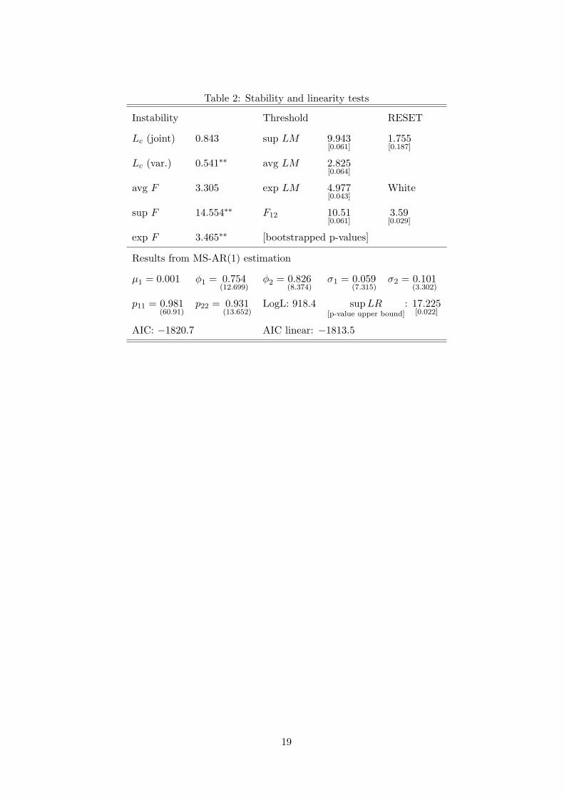
Table 2: Stability and linearity tests

Instability Threshold RESET

Lc (joint) 0.843 sup LM 9.943[0.061]

1.755[0.187]

Lc (var.) 0.541∗∗ avg LM 2.825[0.064]

avg F 3.305 exp LM 4.977[0.043]

White

sup F 14.554∗∗ F12 10.51[0.061]

3.59[0.029]

exp F 3.465∗∗ [bootstrapped p-values]

Results from MS-AR(1) estimation

µ1 = 0.001 φ1 = 0.754(12.699)

φ2 = 0.826(8.374)

σ1 = 0.059(7.315)

σ2 = 0.101(3.302)

p11 = 0.981(60.91)

p22 = 0.931(13.652)

LogL: 918.4 supLR[p-value upper bound]

: 17.225[0.022]

AIC: −1820.7 AIC linear: −1813.5

19

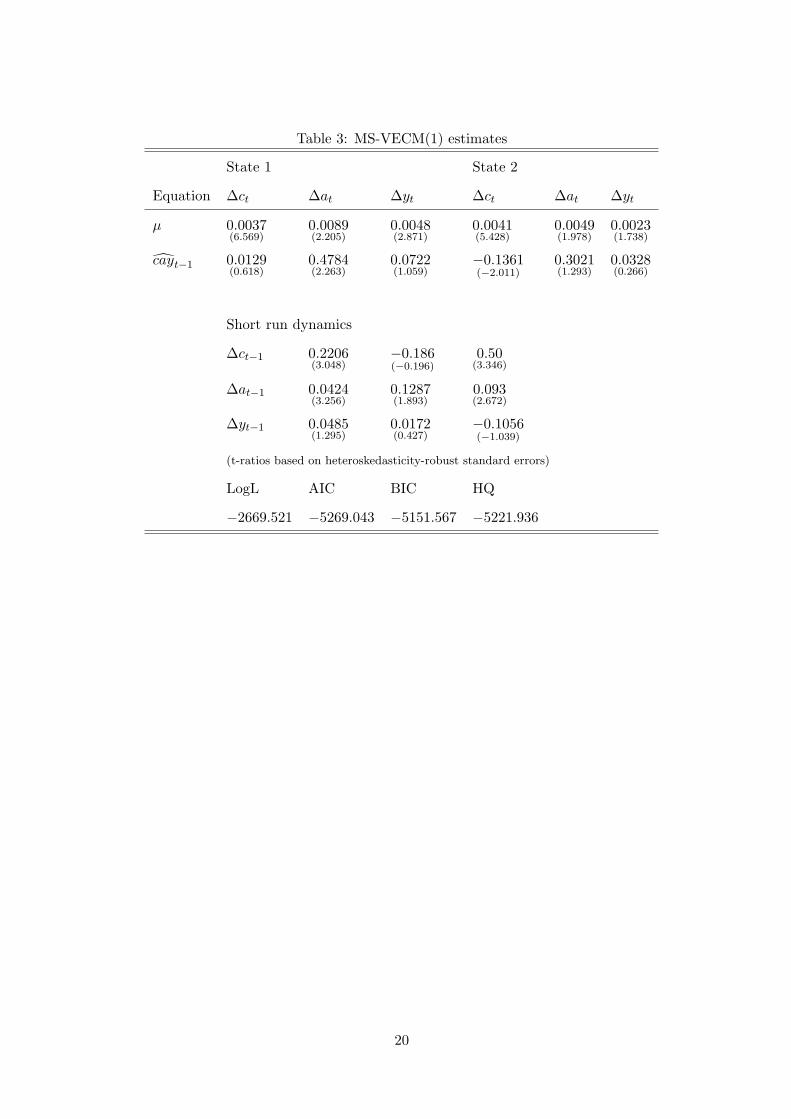
Table 3: MS-VECM(1) estimates

State 1 State 2

Equation ∆ct ∆at ∆yt ∆ct ∆at ∆yt

µ 0.0037(6.569)

0.0089(2.205)

0.0048(2.871)

0.0041(5.428)

0.0049(1.978)

0.0023(1.738)

cayt−1 0.0129(0.618)

0.4784(2.263)

0.0722(1.059)

−0.1361(−2.011)

0.3021(1.293)

0.0328(0.266)

Short run dynamics

∆ct−1 0.2206(3.048)

−0.186(−0.196)

0.50(3.346)

∆at−1 0.0424(3.256)

0.1287(1.893)

0.093(2.672)

∆yt−1 0.0485(1.295)

0.0172(0.427)

−0.1056(−1.039)

(t-ratios based on heteroskedasticity-robust standard errors)

LogL AIC BIC HQ

−2669.521 −5269.043 −5151.567 −5221.936

20

Table 4: Restricted MS-VECM(1) estimates

State 1 State 2

Equation ∆ct ∆at ∆yt ∆ct ∆at ∆yt

cayt−1 − 0.3662(2.166)

− −0.1328(−3.523)

− −

Intercepts and short run dynamics

µ 0.0038(8.43)

0.0071(5.667)

0.003(3.467)

∆ct−1 0.2137(3.007)

−0.100(−0.238)

0.506(3.439)

∆at−1 0.041(3.100)

0.0981(1.572)

0.0823(2.577)

∆yt−1 0.0459(1.115)

0.0172(0.425)

−0.108(−1.032)

p11 = 0.9174(2.415)

p22 = 0.9475(1.99)

(t-ratios based on heteroskedasticity-robust standard errors)

LogL AIC BIC HQ

−2664.319 −5272.637 −5179.457 −5223.952

21

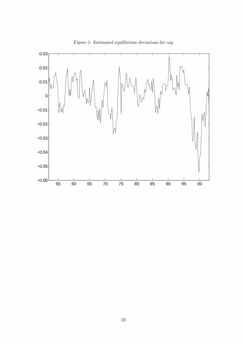
Figure 1: Estimated equilibrium deviations for cay

55 60 65 70 75 80 85 90 95 00−0.06

−0.05

−0.04

−0.03

−0.02

−0.01

0

0.01

0.02

0.03

22

Figure 2: Consumption and asset wealth

10.4

10.6

10.8

11.0

11.2

11.4

11.6

11.8

12.0

Asset wealth

55 60 65 70 75 80 85 90 95 008.8

9.0

9.2

9.4

9.6

9.8

10.0

Consumption

55 60 65 70 75 80 85 90 95 00−0.06

−0.04

−0.02

0

0.02

0.04

0.06

0.08

asset wealth

consumption

23

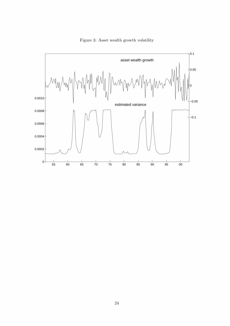
Figure 3: Asset wealth growth volatility

−0.1

−0.05

0

0.05

0.1

asset wealth growth

55 60 65 70 75 80 85 90 95 000

0.0002

0.0004

0.0006

0.0008

0.0010

estimated variance

24

Figure 4: Smoothed probabilities and zt−1

−0.06

−0.04

−0.02

0

0.02

0.04

55 60 65 70 75 80 85 90 95 000

0.2

0.4

0.6

0.8

1

25

Figure 5: MS-VECM smoothed probabilities and zt−1

−0.06

−0.04

−0.02

0

0.02

0.04

55 60 65 70 75 80 85 90 95 000

0.2

0.4

0.6

0.8

1

26