Spatially explicit models of divergence and genome hitchhiking

Spatially explicit models of divergence and genome hitchhiking

S. M. FLAXMAN*, J . L . FEDER† & P. NOSIL*1

*Department of Ecology and Evolutionary Biology, University of Colorado, Boulder, CO, USA

†Department of Biological Sciences, University of Notre Dame, Notre Dame, IN, USA

Keywords:

barriers to gene flow;

coarse-grained;

ecological speciation;

environmental cline;

fine-grained;

gradient;

mosaic habitats.

Abstract

Strong barriers to genetic exchange can exist at divergently selected loci,

whereas alleles at neutral loci flow more readily between populations, thus

impeding divergence and speciation in the face of gene flow. However,

‘divergence hitchhiking’ theory posits that divergent selection can generate

large regions of differentiation around selected loci. ‘Genome hitchhiking’

theory suggests that selection can also cause reductions in average genome-

wide rates of gene flow, resulting in widespread genomic divergence (rather

than divergence only around specific selected loci). Spatial heterogeneity is

ubiquitous in nature, yet previous models of genetic barriers to gene flow

have explored limited combinations of spatial and selective scenarios. Using

simulations of secondary contact of populations, we explore barriers to gene

flow in various selective and spatial contexts in continuous, two-dimen-

sional, spatially explicit environments. In general, the effects of hitchhiking

are strongest in environments with regular spatial patterning of starkly

divergent habitat types. When divergent selection is very strong, the absence

of intermediate habitat types increases the effects of hitchhiking. However,

when selection is moderate or weak, regular (vs. random) spatial arrange-

ment of habitat types becomes more important than the presence of

intermediate habitats per se. We also document counterintuitive processes

arising from the stochastic interplay between selection, gene flow and drift.

Our results indicate that generalization of results from two-deme models

requires caution and increase understanding of the genomic and geographic

basis of population divergence.

Introduction

Genetic differentiation during population divergence and

speciation is often heterogeneous across the genome,

where divergent selection drives or maintains differences

in some regions, whereas the homogenizing effects of

gene flow or insufficient time for random differentiation

by genetic drift preclude divergence in other regions

(Via, 2001; Wu, 2001; Nosil et al., 2009; Nosil & Feder,

2012). These ideas have a long history in studies of

hybrid zones and sympatric speciation (Barton, 1979,

1995, 2001; Barton & Hewitt, 1985; Via, 2001).

However, it is only with recent technical and analytical

advances that allow genetic divergence at many loci to

be screened in most any organism that numerous studies

attesting to the porous nature of the genome have

emerged (e.g. for reviews, see Nielsen, 2005; Nosil et al.,

2009; Strasburg et al., 2012). For example, the last

decade has seen the emergence of many population

genomic studies reporting ‘outlier loci’ whose genetic

divergence exceeds that observed for the rest of the gen-

ome, putatively because such loci are affected (either

directly or indirectly via linkage) by divergent selection

(Beaumont, 2005; Foll & Gaggiotti, 2008; Gompert &

Buerkle, 2011).

These observations have motivated investigations of

intragenomic heterogeneity (with respect to differenti-

ation of loci) during speciation with gene flow. A

recent verbal theory of ‘divergence hitchhiking’

Correspondence: Samuel Flaxman, Department of Ecology and

Evolutionary Biology, University of Colorado, Campus Box 334,

Boulder, CO 80309, USA. Tel.: +1 303 492 7184;

fax: +1 303 492 8699; e-mail: [email protected] address: Department of Animal and Plant Sciences, University

of Sheffield, Sheffield S10 2TN UK

ª 2 01 2 THE AUTHORS . J . E VOL . B I OL . 2 5 ( 2 0 1 2 ) 2 6 33 – 2 6 50

2633JOURNAL OF EVOLUT IONARY B IO LOGY ª 20 1 2 EUROPEAN SOC I E TY FOR EVOLUT IONARY B IO LOGY

doi: 10.1111/jeb.12013

(henceforth ‘DH’) ties the above ideas together to gen-

erate a mechanism by which speciation in the face of

gene flow may be easier than previously thought (Via

& West, 2008; Via, 2009, 2012). The premise is that

divergent selection reduces interbreeding between pop-

ulations in different habitats, for example, by causing

ecologically based selection against immigrants and

hybrids. This reduces interpopulation recombination,

and even if recombination occurs, selection can con-

tinue to reduce the frequency of immigrant alleles by

selecting against advanced-generation hybrids. This

reduction in effective gene flow might allow large

regions of genetic differentiation to build up in the

genome around the few loci subject to strong diver-

gent selection at the initiation of speciation (Gavrilets,

2004).

This idea rests on the assumption that divergent

selection on a site will create a relatively large – with

respect to recombination distance – window of reduced

gene flow around it, enhancing the potential to accu-

mulate differentiation at linked sites. For example, in

host races of pea aphids and in ecotypes of whitefish,

regions of differentiation away from known QTL are as

large as 20 cM (Rogers & Bernatchez, 2007; Via &

West, 2008; Renaut et al., 2012; Via, 2012). In many

other instances, regions of divergence appear much

smaller (Turner et al., 2005, 2010; Machado et al., 2007;

Noor et al., 2007; Turner & Hahn, 2007; Makinen et al.,

2008; Storz & Kelly, 2008; Wood et al., 2008; Baxter

et al., 2010; Counterman et al., 2010; Scascitelli et al.,

2010; Strasburg et al., 2012), for example sometimes

spanning just a few hundred kilobases or < 1 cM

(Nadeau et al., 2012).

As a nonmutually exclusive alternative to DH in a

few genomic regions, speciation may be promoted by

‘multifarious’ selection acting on numerous loci distrib-

uted across the genome (which, for example, affect

many different phenotypic traits: Rice & Hostert, 1993;

Lawniczak et al., 2010; Michel et al., 2010). Indeed, the

direct involvement of many (i.e. tens to hundreds of)

loci in establishing barriers during speciation with gene

flow is expected from empirical as well as theoretical

considerations (Barton, 1983; Barton & Bengtsson,

1986). Reductions in average genome-wide gene flow

due to such multifarious selection could facilitate fur-

ther genetic differentiation, even for loci unlinked to

those under selection, via a process recently termed

‘genome hitchhiking’ (Feder et al., 2012; henceforth

‘GH’). DH and GH are both concerned with effects of

divergent selection. The difference is that whereas DH

focuses on ‘islands’ of differentiation formed around

divergently selected loci due to tight physical linkage,

GH focuses on more genomically widespread conse-

quences arising from reductions in effective migration

rates. These two theories – DH and GH – are compli-

mentary; for example, fortuitous physical linkage of

many loci under multifarious selection could enhance

barriers to gene flow (Barton, 1983; Barton & Bengts-

son, 1986).

We note that the use of the term ‘hitchhiking’ (as part

of both DH and GH) in the work performed here differs

from its classical usage in describing the effects of selec-

tive sweeps within populations (Maynard Smith & Hai-

gh, 1974; Barton, 2000; Charlesworth et al., 2003). Here,

we follow Barton (2000: p. 1553) in using the term to

encompass ‘…indirect effects of selection at one or more

loci on the rest of the genome.’ In this broader sense,

hitchhiking effects may arise not only from selective

sweeps, but also from balanced polymorphisms, local

selection, background selection or selection against

hybrids in a genetic cline (Kaplan et al., 1991; Nordborg

et al., 1996a,b; Charlesworth et al., 1997, 2003; Barton,

2000, 2008).

Despite decades of useful work on hitchhiking and

genetic barriers, additional theory on genomic patterns

of divergence is needed for at least two reasons. First,

debates have arisen about the size and number of geno-

mic ‘islands’ we expect to see during speciation with

gene flow (Via & West, 2008; Feder & Nosil, 2010;

Feder et al., 2012; Via, 2012). Second, much previous

theory in this area has, by necessity, made limiting

assumptions in order to arrive at general (analytic)

expressions describing the dynamics of allele preserva-

tion/loss and evolutionary equilibria. For example,

many spatial models have made one or more of the

following assumptions: (i) there are only two discrete

demes, (ii) there is no intrinsic spatial environmental

variation in fitness, (iii) selection is weak, (iv) allele

frequencies at loci under selection do not fluctuate, (v)

a separation of spatial or temporal scales is possible for

different biological processes, (vi) the environment, if

spatially continuous, is one-dimensional, and/or (vii)

populations are infinite (see Barton, 2000; Charles-

worth et al., 2003 for reviews). Our simulations make

none of these common assumptions.

Recently, Feder & Nosil (2010) used a combination of

analytical and simulation approaches to expand the

single-locus models of Charlesworth et al. (1997) to any

number of loci under selection and to a wider range of

parameter values. Their models considered two demes

subject to divergent selection and exchanging migrants

at a gross rate m. The main finding of Feder & Nosil

(2010) was that DH around a single locus can generate

large regions of neutral differentiation of up to 10 cM

but only under somewhat limited conditions: strong

selection, low effective population size (Ne � 103) and

low migration rates (m � 10�3). Even modest increases

in Ne or m greatly diminished neutral differentiation

around a selected gene. When multiple selected loci are

considered, regions of differentiation were larger. How-

ever, with many loci under selection, effective migra-

tion rates become low enough that genome-wide

divergence of neutral sites occurs via GH and isolated

regions of divergence are erased. What is therefore

ª 20 1 2 THE AUTHORS . J . E VOL . B I OL . 2 5 ( 2 0 12 ) 2 63 3 – 2 65 0

JOURNAL OF EVOLUT IONARY B IOLOGY ª 2012 EUROPEAN SOC I E TY FOR EVOLUT IONARY B IO LOGY

2634 S. M. FLAXMAN ET AL.

https://www.researchgate.net/publication/12200803_Genetic_Hitchhiking?el=1_x_8&enrichId=rgreq-04e2ed40-d678-4758-a4e8-0b36408c3259&enrichSource=Y292ZXJQYWdlOzIzMjc0MDU2MztBUzoxMDE0NTI2NDcyMzk2ODRAMTQwMTE5OTYwNDQzOA==

https://www.researchgate.net/publication/13781904_Charlesworth_B_Nordborg_M_Charlesworth_D_The_effects_of_local_selection_balanced_polymorphism_and_background_selection_on_equilibrium_patterns_of_genetic_diversity_in_subdivided_populations_Genet_Res_?el=1_x_8&enrichId=rgreq-04e2ed40-d678-4758-a4e8-0b36408c3259&enrichSource=Y292ZXJQYWdlOzIzMjc0MDU2MztBUzoxMDE0NTI2NDcyMzk2ODRAMTQwMTE5OTYwNDQzOA==

https://www.researchgate.net/publication/51925460_Via_S_Divergence_hitchhiking_and_the_spread_of_genomic_isolation_during_ecological_speciation_with_gene_flow_Philos_Trans_R_Soc_Lond_B_Biol_Sci_367_451-460?el=1_x_8&enrichId=rgreq-04e2ed40-d678-4758-a4e8-0b36408c3259&enrichSource=Y292ZXJQYWdlOzIzMjc0MDU2MztBUzoxMDE0NTI2NDcyMzk2ODRAMTQwMTE5OTYwNDQzOA==

https://www.researchgate.net/publication/51925450_Genomic_islands_of_divergence_in_hybridizing_Heliconius_butterflies_identified_by_large-scale_targeted_sequencing?el=1_x_8&enrichId=rgreq-04e2ed40-d678-4758-a4e8-0b36408c3259&enrichSource=Y292ZXJQYWdlOzIzMjc0MDU2MztBUzoxMDE0NTI2NDcyMzk2ODRAMTQwMTE5OTYwNDQzOA==

https://www.researchgate.net/publication/51925461_Establishment_of_new_mutations_under_divergence_and_genome_hitchhiking?el=1_x_8&enrichId=rgreq-04e2ed40-d678-4758-a4e8-0b36408c3259&enrichSource=Y292ZXJQYWdlOzIzMjc0MDU2MztBUzoxMDE0NTI2NDcyMzk2ODRAMTQwMTE5OTYwNDQzOA==

https://www.researchgate.net/publication/51385928_The_Genetic_Architecture_of_Ecological_Speciation_and_the_Association_with_Signatures_of_Selection_in_Natural_Lake_Whitefish_Coregonus_sp_Salmonidae_Species_Pairs?el=1_x_8&enrichId=rgreq-04e2ed40-d678-4758-a4e8-0b36408c3259&enrichSource=Y292ZXJQYWdlOzIzMjc0MDU2MztBUzoxMDE0NTI2NDcyMzk2ODRAMTQwMTE5OTYwNDQzOA==

required for DH to be important is that effective gene

flow is significantly reduced locally in the genome

without being substantially reduced globally. As an

extension of this initial work, Feder et al. (2012) con-

sidered the potential for further differentiation to accu-

mulate and reproductive isolation to increase after

equilibrium was achieved via the establishment of new

ecologically beneficial mutations causing habitat-associ-

ated fitness trade-offs. They found that the strongest

predictor of mutation establishment was the strength of

selection acting on the new mutation (relative to the

migration rate), but with both DH and GH having more

minor secondary effects under some conditions. None-

theless, when a few strongly selected loci establish, GH

can have important consequences for facilitating muta-

tion establishment, whereas the effects of DH again

appeared to be limited to new mutations occurring in

close proximity (e.g. within 1 cM) of an already

strongly selected gene.

Motivated by the fact that spatial heterogeneity is

ubiquitous in nature, we here expand past work on DH

and GH to a much wider range of spatial and selective

scenarios using individual-based, spatially explicit

models. Specifically, our simulations consider the main-

tenance of neutral variation in scenarios that mimic the

set-up of previous models of genetic clines and intro-

gression during secondary contact (e.g. Barton, 1983).

The work thus addresses not only issues concerning

genomic divergence, but also classical and ongoing

debates concerning how the spatial arrangement of

populations affects population differentiation (Mayr,

1963; Felsenstein, 1981; Via, 2001; Berlocher & Feder,

2002; Bolnick & Fitzpatrick, 2007; Fitzpatrick et al.,

2008; Mallet et al., 2009). For example, a major consid-

eration for the geography of speciation is whether

environmental features change abruptly in space (e.g.

discrete patches of different host plant species) or con-

tinuously along gradients, resulting in geographic clines

(Endler, 1977).

To be sure, there are a number of previous investiga-

tions that directly compared the results from multiple

different spatial scenarios (Barton, 1983, 2008; Barton

& Bengtsson, 1986; Charlesworth et al., 2003). Our

work extends that past work by considering a combina-

tion of realistic, biologically important features: distinct

and variable individuals, drift arising naturally as a

consequence of stochasticity in both migration and

reproduction, selective pressures that vary in space and

meiosis with stochastic recombination events. Although

past models have considered some of these factors in

concert, to our knowledge, no previous model of

genetic barriers and secondary contact has included all

of them simultaneously. Among these factors, we focus

a great deal on the role of spatial environmental

variation because very few previous works have

included true, continuous, bounded two-dimensional

environments (Charlesworth et al., 2003; Doebeli &

Dieckmann, 2003; Wilkins, 2004; Barton, 2008), yet

such environments typify a great deal of the terrestrial

species on this planet. Considering two-dimensional

space is not merely biologically relevant; conclusions

derived from two-dimensional models can often differ

from their one-dimensional analogues (Doebeli &

Dieckmann, 2003; Wilkins, 2004; Barton, 2008).

Our results about the influences of recombination

rates and the overall strength of selection on genetic

barriers, DH and GH are consistent with the extensive

past work cited above. However, we also found

pronounced, nonintuitive effects of the other factors

examined. Additionally, our results have implications

for empirical studies of the gene regions involved in

adaptation and speciation (Nielsen, 2005; Noor & Feder,

2006; Stinchcombe & Hoekstra, 2008). For example,

our results strongly suggest that neutral ‘outlier’ loci

reflect the presence of (unidentified) genes under selec-

tion that are very closely linked to the outlier (or the

outliers are false positives), rather than long-distance

effects of DH.

Materials and methods

Our results were generated from a stochastic, individ-

ual-based computer simulation model. The model was

written in the C programming language, using the

Mersenne Twister (DSFMT version 2.1: Saito & Matsum-

oto, 2006) to generate random numbers in the simula-

tions. Source code for simulations is archived at http://

sourceforge.net/projects/spatialhitchhik/files/. Spread

sheets of parameter combinations used, raw data and

metadata are archived on Dryad (doi:10.5061/

dryad.8sc8b).

Although general, analytic results are desirable, use-

ful analytic results are not always attainable in models

with the multiple facets of biological realism we incor-

porated (Charlesworth et al., 1997, 2003; Doebeli &

Dieckmann, 2003). For example, diffusion approxima-

tions may break down when selection is strong or

when there are small, varying numbers of individuals

(by chance) within a deme (Barton & Bengtsson,

1986). Indeed, due to the combination of genetic and

spatial structure in our model, simplifying to the extent

necessary to derive useful analytic results would result

in a fundamentally different model that left out one or

more of the factors we wish to consider. However, the

parameter space of our model is not so large as to pre-

vent rigorous examination of all of these factors

through simulations. Additionally, by running simula-

tions without any selection (explained below), we were

able to numerically infer null statistics as points of

reference for measuring the importance of DH and GH.

The model considers a population of constant size

consisting of N diploid, hermaphroditic, obligately out-

crossing individuals that migrate and reproduce in a

continuous, spatially explicit and variable environment.


JOURNAL OF EVOLUT IONARY B IO LOGY ª 20 1 2 EUROPEAN SOC I E TY FOR EVOLUT IONARY B IO LOGY

Spatial models of hitchhiking 2635

https://www.researchgate.net/publication/22732027_Geographic_Variation_Speciation_and_Clines_MPB-10?el=1_x_8&enrichId=rgreq-04e2ed40-d678-4758-a4e8-0b36408c3259&enrichSource=Y292ZXJQYWdlOzIzMjc0MDU2MztBUzoxMDE0NTI2NDcyMzk2ODRAMTQwMTE5OTYwNDQzOA==

https://www.researchgate.net/publication/51925461_Establishment_of_new_mutations_under_divergence_and_genome_hitchhiking?el=1_x_8&enrichId=rgreq-04e2ed40-d678-4758-a4e8-0b36408c3259&enrichSource=Y292ZXJQYWdlOzIzMjc0MDU2MztBUzoxMDE0NTI2NDcyMzk2ODRAMTQwMTE5OTYwNDQzOA==

An individual in the model was defined by its genotype

of Λ diploid loci, where Λ = 13, 14 or 22 for the results

presented here (Table 1). Two distinct alleles segregated

at each locus, represented by ‘0’ and ‘1’. Loci were

arrayed along linear chromosomes, and an individual’s

first locus (denoted L0) was always under selection. The

next 11 loci, denoted L1, L2, …, L11, were linked to L0at recombination distances [r1, r2, …, r11] = [0.00001,

0.00002, 0.00005, 0.0001, 0.0002, 0.0005, 0.001, 0.005,

0.01, 0.05, 0.5]. We considered an additional locus, L12,

unlinked to any of the other loci (on a different chro-

mosome; either allele inherited with probability 0.5).

Recombination distance, rj, was defined as the probabil-

ity that a crossover event would occur during a round

of meiosis anywhere between locus L0 and Lj (from 0

to j crossovers could occur). For all the results shown

below, the loci L1, L2, …, L12 were neutral. When

selected loci in addition to L0 were included in the

simulations, they were unlinked to each other and to

all other loci. In summary, our simulations considered

the fates of alleles at 12 neutral loci, when l = 1, 2 or

10 additional loci were under selection.

The environment was defined in terms of a two-

dimensional unit square, with the ith individual’s loca-

tion represented by its Euclidean coordinates (xi, yi) in

the square (i.e. xi, yi ∊ [0, 1]), the boundaries of which

were treated as fixed, impermeable barriers. The model

utilizes discrete time, with each time step representing

a generation. A generation consisted of migration by all

individuals followed by reproduction, with selection,

recombination and drift modelled as part of the repro-

ductive process. Generations were nonoverlapping, and

thus at the end of one generation, the N individuals

were replaced by N offspring (details below). Offspring

were born into the same patch as their parents at ran-

dom locations (with respect to their parents’ locations).

Each run of the model lasted 106 generations or until

fixation of one allele had occurred at all neutral loci

(L1, …, L12), whichever came first.

Migration in the model was cost-free and random in

direction and distance travelled (normally distributed

with mean 0 and standard deviation r). Movements

were truncated (when necessary) to keep individuals

within the borders of the unit square. With the param-

eters used below, the average gross migration rate

(probability of patch switching per individual per gener-

ation) that emerged from the model ranged from ~0.02to ~0.15 (see Fig. S1, Supporting Information), depend-

ing upon the granularity of the environment. In con-

junction with the range of selection strengths we used

(given below), we had cases in which gross migration

rates were less than, equal to or greater than the

strength of selection.

Recombination, selection and drift were modelled to

occur during reproduction, as follows. An individual’s

fitness depended upon its genotype, its location and the

fitness scheme. For the purposes of representing spatial

variation in the environment, the overall environment

was considered to be composed of an n 9 n set of

square patches (demes), all of equal size (Fig. 1). We

show the results below for n = 3 and 9, that is, nine

and 81 patches. Hence, a scenario with nine large

patches (each with area �11% of the unit square)

represents a ‘coarse-grained’ environment, whereas a

scenario with 81 smaller patches (each with area

�1.2% of the unit square) represents a more ‘fine-

grained’ environment.

We considered three different types of spatial varia-

tion in fitness: (i) a regular ‘gradient’ of fitness across

patches (Fig. 1a,d), (ii) a ‘grey-scale mosaic’ having the

same numbers and types of patches as the ‘gradient,’

but with their locations randomized (Fig. 1b,e), and

(iii) an ‘extreme mosaic’ of two very different patch

types (Fig. 1c,f). Comparing the results from a gradient

with those from a grey-scale mosaic allowed us to

determine the influence of the spatial arrangement of

patches. Comparing the results from the grey-scale

mosaic with the extreme mosaic gave insights into the

Table 1 Variables and parameter values used in simulations.

Variable/parameter Meaning Value(s) or range used*

N Total number of individuals in environment 1000, 5000, 10000

Λ Total number of loci in a genome 13, 14, 17, 22

l Number of loci under selection 1, 2, 5, 10

Lj Locus j j = 0, 1, …, Λ�1

rj Probability of recombination between L0 and Lj 11 different values (see text)

D Dimensionality of habitat 1 (unit line) or 2 (unit square)

nD Number of patches in habitat 2, 3, 4, 9, 11, 25, 49, 81, 121

Smax Maximum value of selection coefficient 0.01, 0.1, 0.5

r Standard deviation of migration movement distances (normalized to unit line) 0.01, 0.02, 0.05

d Threshold for identifying when Lj (j > 0) was decoupled from locus L0 0.001, 0.1

q Threshold for identifying when Lj (j > 0), previously decoupled, had been ‘rescued’ 10�5, 10�9

*Values shown in this column are those we explored in parameter studies and sensitivity analyses. Values shown in boldface are repre-

sented in results shown here.




importance of the presence or absence of intermediate

habitats.

The individuals within the boundaries of a single

patch constituted the mating pool for that patch, from

which gametes were drawn stochastically. The probabil-

ity that an individual was selected to contribute a gam-

ete to an offspring was proportional to the individual’s

fitness relative to the fitness of all other individuals in

the same patch. For scenarios with just a single locus

(L0) under selection, the maximum fitness a genotype

could have was 1.0 + Smax, where Smax = 0.01, 0.1 or

0.5, and the minimum fitness it could have was 1.0. In

‘extreme mosaic’ spatial scenarios, the fitness of an

individual homozygous at L0 was thus either 1.0 or

1.0 + Smax, depending upon the patch type (Fig. 1c,f),

and the fitness of individuals that were heterozygous at

L0 was 1.0 + 0.5Smax (i.e. intermediate) in all patches.

In ‘gradient’ spatial scenarios with a single locus

under selection, an individual homozygous for the ‘0’

allele at L0 had maximum fitness (1.0 + Smax) in the

upper row of patches (Fig. 1a,d). To create the ‘gradi-

ent’, moving one row ‘down’, the fitness of this (0,0)

homozygote is decreased by Smax/(n�1), such that it

would have minimum fitness (1.0) in the bottom row

of patches of the habitat and intermediate fitness (1.0 +0.5Smax) in the middle row of patches (Fig. 1a,d). The

fitness of an individual homozygous for the ‘1’ allele at

L0 was the reverse of that just described. Finally, in the

‘gradient’ scenarios with a single locus under selection,

individuals that were heterozygous at L0 were assumed

to have maximum fitness (1.0 + Smax) in the middle

row of patches, that is, in the intermediate environ-

ment where the two homozygotes had the same fitness.

As we move away from that row (up or down), the fit-

ness of a heterozygote decreases by Smax/(n�1), such

that heterozygotes have intermediate fitness

(1.0 + 0.5Smax) in the top and bottom rows (i.e. where

homozygotes were most strongly favoured). We note

that these assumptions created overdominance in inter-

mediate patch types in the gradient scenarios. We ran

other simulations of gradients in which heterozygote

fitness was constant across all patches (as it was in

the extreme mosaic scenario). The results from the

latter did not change our conclusions about mosaic

(a) (b) (c)

(d) (e) (f)

Fig. 1 Spatial fitness schemes in the three types of environments in the model. In all panels, shading represents the fitness contribution of

a locus that is under selection and is homozygous for the ‘1’ allele. Black represents the maximum possible contribution to fitness

(1.0 + Smax for single locus and multiplicative fitness;ffiffiffiffiffiffiffiffiffiffiffiffiffiffiffiffiffiffiffiffiffiffi

1:0þ Smaxlp

for ‘root’ fitness; see Materials and Methods), and white represents the

minimum possible contribution (1.0) to fitness. Fitness contributions are exactly the reverse for selected loci homozygous for the ‘0’ allele.

(a–c) show ‘coarse-grained’ habitats; (d–f) depict ‘fine-grained’ variation. (a) and (d) depict gradients of fitness from the top to the bottom

of the habitat; (b) and (e) depict a random mosaic with the same numbers and types of patches as the gradient; (c) and (f) depict random

mosaics composed of two extreme patch types.




vs. gradient environments (see Fig. S4, Supporting

Information).

We also investigated how increasing the numbers of

unlinked loci under selection influenced the potential

for hitchhiking to maintain neutral variation. For mul-

tiple loci, we considered all selected loci to contribute

equally to fitness, with the fitness of a genotype calcu-

lated as the product of fitness contributions across all

loci under selection. We performed the calculation of

this product in two different ways. (i) In our ‘root’ fit-

ness scheme, the maximum possible fitness contribu-

tion that a selected locus could make wasffiffiffiffiffiffiffiffiffiffiffiffiffiffiffiffiffiffiffiffiffiffi

1:0þ Smaxlp

,

where l was the number of loci under selection. Thus,

in this ‘root’ fitness scheme, as l was increased, a given

overall level of selection (specified by a given value of

Smax) was constant but was spread out over increasing

numbers of unlinked loci on different chromosomes

across the genome. (ii) In our ‘multiplicative’ fitness

scheme, the maximum possible fitness contribution

from each selected locus was 1.0 + Smax. Thus, under

the multiplicative scheme, the addition of each new

locus increased the total strength of selection possible

by a factor of 1.0 + Smax (i.e. maximum potential

strength of selection = 1:0þ Smaxð Þl). In both the ‘root’

and ‘multiplicative’ fitness schemes, the calculation of

the contribution of each locus to fitness for mosaic vs.

gradient environments was accomplished as described

above for the single-locus case (see also Fig. 1). We

note that the multiplicative scheme with l = 10 and

Smax = 0.5 leads to selection strengths that are unrealis-

tically large; our purpose in presenting them is solely to

demonstrate just how strong selection would have to

be in order to see long-distance effects of hitchhiking

on neutral loci.

The model was initialized with (1) N/2 = 2500 indi-

viduals homozygous at every locus for ‘0’ alleles, all

starting at the ‘top’ of the unit square environment,

and (2) N/2 = 2500 additional individuals homozygous

at every locus for ‘1’ alleles, all starting at the ‘bottom’

of the environment. These initial conditions simulated

an evolutionary scenario akin to that used in many

previous theoretical studies: allopatric populations with

fixed differences at a number of loci (neutral and

selected) followed by secondary contact. Thus, our

model focuses on the maintenance of neutral differenti-

ation, and future work will explore the origin of differ-

entiation from new mutations.

Examining the efficacy of DH and GH: the loss ofneutral alleles

For the 12 neutral loci L1, L2, …, L12, we examined the

preservation of genetic variation in the face of gene flow

and recombination. Specifically, we tracked how many

generations it took for either the ‘0’ or ‘1’ allele to be lost

at each neutral locus, which we henceforth refer to as

‘fixation times’. This is somewhat similar to studying a

coalescent process in a subdivided population with link-

age, recombination, selection and drift (e.g. Kaplan et al.,

1991). We recorded fixation times for 1000 independent

initializations for each parameter combination and

explored if and how these fixation times varied under

different parameter combinations. If fixation did not

occur at a locus by the end of a simulation run, then it

was noted as such. Fixation times for neutral loci in the

absence of any selection (Smax = 0) reflect the ‘null’

expectations for the maintenance of prestanding genetic

variation and differentiation following secondary contact

and gene flow. These null expectations appear below as

dashed horizontal lines in Figs 2–5. Increases in fixation

times above these baseline values reflect the potential

for hitchhiking to preserve neutral differentiation. Spe-

cifically, increases for only those neutral loci that are

linked to a selected locus indicate the potential for DH to

maintain prestanding neutral divergence following

secondary contact. Increases in fixation times because of

selection on an unlinked locus reflect the potential for

GH. Because we simulated many independent replicates

of the same scenario, we were also able to evaluate the

extent that different loci might evolve independently by

examining the correlations among loci in their fixation

times.

The dynamics of divergence and loss at differentloci

We also calculated FST values among patches for each

locus using the standard formula FST ¼ HT�HS

HT, where HT

was the total observed heterozygosity at a given locus

at a given time step and HS was the expected heterozy-

gosity based upon each patch’s observed heterozygosity

(Hartl & Clark, 2007). FST,t,j denoted the FST value for a

given locus number j at time t. When an allele at

neutral locus Lj was perfectly linked to an allele at the

selected locus L0, their FST values were identical (FST,t,j= FST,t,0). However, as these alleles became decoupled

from one another due to gene flow and recombination,

their FST values diverged. In particular, over time FST,t,0is expected to reach a quasi-steady-state (as shown

below) representing migration–selection balance. How-

ever, once decoupled from the selected locus, FSTvalues for neutral loci should be less than those for the

selected locus and eventually decay to zero as one allele

goes to fixation (by chance). Hence, we recorded time

series of FST values for each locus.

These time series revealed some surprising dynamics

of allele preservation and loss. In particular, the

combined forces of recombination, selection and drift

interacted to produce many cases in which the neutral

locus became partially decoupled from the selected

locus (i.e. 0 < FST,t,j < FST,t,0), sometimes to a great

extent (i.e. 0 < FST,t,j << FST,t,0). However, rather than

FST,t,j continuing steadily to zero from this point, the

neutral locus could also become recoupled in linkage




disequilibrium to an allele at the selected locus, with

FST,t,j rising again to higher levels. At the start of a run,

every ‘1’ allele at locus Lj (1 � j � 11) was found on

a chromosome with a ‘1’ allele at L0, but after sufficient

rounds of recombination and reproduction, some frac-

tion x of the ‘1’ alleles at Lj would be on chromosomes

with a ‘0’ allele at L0, generally reducing FST,t,j. If effec-

tive recombination rates were low enough, however, x

could decline from this point to zero (due to drift),

resulting in a steady rise of a ‘1’ allele at Lj being

associated with a ‘1’ allele at L0 and FST,t,j rising. We

refer to cases of the latter as ‘rescues’ of the alleles at

the neutral locus, because the differentiation at the

neutral locus that was present at the beginning of the

run is restored. Like fixation time, the frequency of

rescues also reflects the potential for hitchhiking to

maintain population differentiation, and thus, we

explored the parameters affecting rescues. The reason

that ‘rescues’ reflect such potential is that they reflect

effective recombination rates, in the following ways:

(i) when effective recombination is close to zero, there

is nothing to be rescued; (ii) when effective recombi-

nation rates are low, rescues should be possible

and observed; finally, (iii) when effective recombina-

tion rates are larger than the rate of neutral allele

frequency change due to drift, rescues will be rare

or impossible, because recombination will break

associations between alleles faster than they can be

rescued.

In order to identify rescues, we needed to establish

objective criteria for identifying both (i) a ‘decoupling

threshold’ when a neutral locus could be classified as

having become decoupled from L0, and (ii) a ‘rescue

threshold’ when a locus, having previously become

decoupled, subsequently was rescued. In order to be

conservative in the identification of rescues, we report

the results for a decoupling threshold, d, of FST,t,0�FST,t,j� d = 0.1, and a rescue threshold, q, of FST,t,0�FST,t,j� q = 10�9. To identify a rescue event, we additionally

required that FST,t,0�FST,t,j � q for two consecutive

generations. Rescue events could only follow a decou-

pling, with only one rescue event associated with each

decoupling event. Likewise, only a single decoupling

event was considered possible after each rescue. We

document below that rescues under these criteria were

relatively common, but if less conservative criteria were

(a) (b) (c)

(d) (e) (f)

Fig. 2 Median fixation times (logarithmic scale) for 12 neutral loci when a single locus (L0) is under three different levels of selection

(Smax) for gradient (a, d), grey-scale mosaic (b, e) and extreme mosaic (c, f) spatial patterns of environmental variation. Recombination

rates (rj) of the 12 neutral loci to L0 are given on the x-axis on a logarithmic scale (i.e. �5 = recombination rate of 10�5). Results for L12,

the unlinked neutral locus on a separate chromosome, are labelled ‘unl.’ Upper panels (a–c) present results with nine patches, whereas

lower panels (d–f) present results for 81 patches. The ‘null expectation’ when there is no selection on L0 is denoted by the dashed line

(obtained numerically by setting Smax = 0 with all other parameters the same as for the other lines in a panel). Each point is the median of

results of 1000 independent simulation replicates.




used to diagnose rescues, rescues would be even more

common (results not shown).

Results

As expected from previous theory, recombination dis-

tance (rj) and the strength of selection (Smax) had strong

effects on fixation times. Stronger selection (higher val-

ues of Smax) led to longer fixation times, and as recombi-

nation distance increased from very low (r1 = 10�5) to

high levels (r11 = 0.5), the median time to fixation

decreased by one to two orders of magnitude (Figs 2–4).However, in nearly all parameter combinations, this

decreasing trend was almost entirely due to the fixation

times of the six loci most tightly linked to the selected

locus L0 with rj � 0.0005. Under most circumstances,

rj � 0.001 (�3 on the log scale) resulted in median

fixation times that were not substantially longer than

(a) (b) (c)

(d) (e) (f)

(g) (h) (i)

(j) (k) (l)

Fig. 3 Median fixation times when either (a–f) two or (g–l) 10 loci are under selection and the strength of selection is given by the ‘root’

fitness calculation (see Materials and Methods). Numbers of patches, spatial scenario and fitness scheme are given above each panel. Other

details are as in Fig. 2.




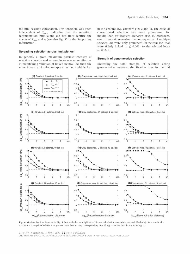
the null baseline expectation. This threshold was often

independent of Smax, indicating that the selection/

recombination ratio alone did not fully capture the

effects of Smax and rj (see also Fig. S5 in the Supporting

Information).

Spreading selection across multiple loci

In general, a given maximum possible intensity of

selection concentrated on one locus was more effective

at maintaining variation at linked neutral loci than the

same intensity of selection spread across multiple loci

in the genome (i.e. compare Figs 2 and 3). The effect of

concentrated selection was more pronounced for

mosaic than for gradient scenarios (Fig. 3). Moreover,

even in mosaic scenarios, the consequences of multiple

selected loci were only prominent for neutral loci that

were tightly linked (rj � 0.001) to the selected locus

L0 (Fig. 3).

Strength of genome-wide selection

Increasing the total strength of selection acting

genome-wide increased the fixation time for neutral

(a) (b) (c)

(d) (e) (f)

(g) (h) (i)

(j) (k) (l)

Fig. 4 Median fixation times as in Fig. 3, but with the ‘multiplicative’ fitness calculation (see Materials and Methods). As a result, the

maximum strength of selection is greater here than in any corresponding line of Fig. 3. Other details are as in Fig. 3.




loci linked to L0 (Fig. 4). In cases of the strongest

genome-wide selection simulated with 10 loci having

Smax = 0.5 (Fig. 4g–l), fixation times were elevated for

all neutral loci in the extreme mosaic, including those

unlinked to L0 (although we note that the latter case

involves extremely strong selection that is unlikely to be

observed in natural systems). Indeed, fixation did not

occur within 106 generations in a majority of cases for

most linked neutral loci (see points at 106 for Smax = 0.5

in Fig. 4i,l). The effect of strong genome-wide selection

was also more pronounced for the extreme mosaic than

either of the other spatial scenarios.

Spatial factors: coarse- vs. fine-grainedenvironments

In nearly all cases, the graininess of the environment

had a consistent effect on median fixation time: within

a given parameter set, coarse-grained environments

(fewer, larger patches) had fixation times that were

longer than or equal to those for fine-grained environ-

ments (a greater number of smaller-sized patches;

Figs 2–4). There were a few exceptions to this pattern

at the weakest level of selection (e.g. compare triangles

in Fig 2c,f).

Spatial factors: spatial arrangement of patches andthe presence of intermediate patch types

The effects of spatial arrangement and patch types

depended upon both the strength of selection and

the graininess of the environment. With moderate to

strong selection, the grey-scale mosaic consistently

produced the shortest fixation times across all scenar-

ios. The extreme mosaic produced the longest fixation

times in coarse environments with the strongest lev-

els of selection (e.g. compare squares in Fig. 2a–c;Fig. 3a–c; Fig. 4a–c). However, when selection was

weak and/or the environment was fine-grained,

gradient environments produced the longest fixation

times.

Variance in fixation times

Variances in median fixation time were not large

for loosely linked neutral loci and were similar to

the baseline null level for an unlinked neutral

locus (L12) on a separate chromosome. Moreover,

variance decreased with increasing recombination

distance of the neutral loci from the selected locus L0(Fig. 5).

(a) (b) (c)

(d) (e) (f)

Fig. 5 Variances in observed fixation times for cases with a single locus under selection. Sample sizes, simulation runs used, parameters

and arrangement of panels are all as in Fig. 2. Note that patterns in variance qualitatively mirror the patterns in fixation times (compare

lines here with corresponding panels in Fig. 2). The same was true for variances observed in cases with multiple loci under selection

(results not shown). Variance estimates will be artificially low for parameter combinations and loci that had many runs reaching 106

generations (e.g. panel c) before fixation occurred at a locus because the distribution of fixation times was truncated in such cases

(see Materials and Methods).




Correlations among fixation times

Analysis of correlations among fixation times for neu-

tral loci implied that, in general, there was much

opportunity for even tightly linked neutral loci to

evolve independently of one another. Figure 6 shows

the extent to which neutral alleles at L1 tended to share

the same evolutionary trajectory as alleles at other neu-

tral loci (L2, …, L12), as demonstrated by correlations in

the fixation times between pairs of loci. Correlations for

other focal loci besides L1 showed qualitatively similar

patterns (results not shown). Loci that were very close

together indeed often showed significant correlations

among fixation times, suggesting that very tightly

linked neutral loci could sometimes behave somewhat

as a single ‘gene’. However, correlations were generally

insignificant for any pairwise comparison of fixation

times involving loci L8 through L11 (with rj � 0.005)

compared with any other locus. Thus, even for loci sep-

arated by a recombination frequency as little as 0.5 cM,

evolutionary fates were usually not strongly linked.

FST time series and ‘rescues’

Rescue events (see Materials and Methods) were com-

monly observed in the simulations; an example of mul-

tiple rescues occurring within one run is shown in

Fig. 7 (see Fig. S3 in the Supporting Information for

additional examples). The frequency of rescues varied

with the strength of selection, spatial scenario and

recombination distance. In general, rescues were extre-

mely rare or nonexistent with weak selection

(Smax = 0.01; Fig. 8d–f,j–l). This was due to a relatively

high effective recombination rate in such cases and due

to the fact that the selected alleles themselves could be

lost by being overwhelmed by migration. In contrast,

when selection was strong (Smax = 0.5; Fig. 8a–c,g–i),even relatively large decoupling events could be res-

cued. The frequency of rescues was also greatly affected

by recombination distance. In general, rescues were

much more common for tightly than for loosely linked

loci (but see Fig. 8i, discussed below). Indeed, in the

majority of cases, rescues were very rare for rj > 0.005.

For parameter values in which rescues were common

for at least some loci (i.e. Smax = 0.5), we also exam-

ined the probability of rescue following a decoupling

(Fig. 9). As expected, for a given decoupling criterion,

rescues were more likely for loci that were more tightly

linked to the selected locus. These results were consis-

tent with the findings for fixation time in implying that

the conditions for DH to help maintain, accumulate

and resurrect (rescue) neutral differentiation may be

generally limited to tight linkage and strong, localized

selection acting on the genome.

Discussion

Our work is distinguished from previous theory by con-

sidering the combination of (i) a wide array of spatial

scenarios of intrinsic environmental variation in fitness

(ii) in explicit two-dimensional, bounded space where

(iii) both selection and a number of realistic sources of

stochasticity determine evolutionary trajectories of (iv)

various numbers of selected and neutral alleles. While

including all of these features in our model made ana-

lytic treatment intractable, we were able to investigate

a wide range of biologically relevant scenarios by

simulation. This allowed us to expand past two-deme

models (Feder & Nosil, 2010; Feder et al., 2012) of

hitchhiking to a wider range of geographic scenarios.

In order to quantify the efficacy of hitchhiking,

we considered a starting point that was maximally

Fig. 6 Correlation coefficients among fixation times between L1and all other neutral loci. There are 125 correlation coefficients

per box-and-whisker plot, where each correlation coefficient was

calculated from approximately 200 independent simulation runs.

Boxes show the median (centre line) and interquartile range (IQR;

box). Whiskers span points up to 1.5 IQR beyond the IQR, and ‘+’symbols show data points beyond the latter range.

0 2 4 6

x 104

0

0.25

0.5

0.75

1

Time step (generation)

FS

T

L0

L3

Fig. 7 An example of FST time series for the selected locus (L0)

and a neutral locus (L3) during one run of the model. Downward-

pointing triangles indicate times when decoupling occurred;

upward-pointing triangles indicate the occurrence of a ‘rescue’

event following decoupling (see Materials and Methods). In the

example shown here, L3 is decoupled five times from L0, each of

which is eventually followed by a rescue. However, after the 6th

decoupling, fixation occurs at L3 (line for L3 goes to zero after

63 926 generations).




favourable to the maintenance of neutral differentia-

tion; namely, each neutral allele was perfectly associ-

ated with a selected allele(s), initial populations were

strictly homozygous at all loci considered, and all

individuals began in spatial locations that were favour-

able for their respective genotypes. We then measured

the efficacy of hitchhiking in terms of how many

generations were required for differentiation at each

neutral locus to decline and be lost. This set-up specifi-

cally explored the effectiveness of forces that may pro-

mote DH and/or GH in preventing the loss of neutral

divergence. Furthermore, it also enabled us to build

upon the rich literature of previous theory on barriers

to gene flow during secondary contact.

The roles of the strength of selection and recombina-

tion rates have been extensively explored, and our

results on these factors mirror those of previous work.

Briefly, strong selection and low recombination rates

were required for any noticeable increase in the main-

tenance of neutral variation (relative to the null case of

the absence of selective barriers). These results are

consistent with past models demonstrating the efficacy

of recombination in breaking up linkage disequilibrium

(Felsenstein, 1981; Bolnick & Fitzpatrick, 2007). Quan-

titatively, linkage had to be extremely tight for a barrier

to be effective. Our results agree with previous studies

of hitchhiking in panmictic populations, which showed

that hitchhiking effects are essentially absent for loci

(a) (b) (c)

(d)

(g)

(j) (k) (l)

(h) (i)

(e) (f)

Fig. 8 Observed numbers of rescue events at each neutral locus as a function of model parameters. Decoupling and rescue thresholds

were, respectively, d = 0.1 and q = 10�9 (see Materials and Methods), and in all panels, there were nine patches (coarse environment).

(a–f): a single locus (L0) is under selection. (g–l): 10 loci under selection with the ‘multiplicative’ fitness calculation method. Each boxplot

shows the results from 1000 independent simulation runs (see Fig. 6 for explanation of box-and-whisker plots). Note that the y-axis is

logarithmic.




having rj > 0.1 Smax (Maynard Smith & Haigh, 1974;

see also Fig. S5). However, our results on the roles of rjand Smax were not explained just by the rj/Smax ratio.

We varied Smax over 1.5 orders of magnitude, and we

varied the total strength of selection over more than

two orders of magnitude. Yet, in nearly all scenarios,

any locus that was 0.1 cM or farther from a selected

locus (i.e. rj � 10�3) showed no increase in fixation

time relative to the null case. In Fig. S5, we re-plotted

data from the single-locus case (Fig. 2), as a function of

the rj/Smax ratio; the lack of overlap of lines for differ-

ent Smax values indicates that the rj/Smax ratio does not

explain all the effects of rj and Smax.

The only pronounced cases of hitchhiking effects

beyond 0.1 cM were for the most extreme strengths of

genome-wide selection (Fig. 4g–l). However, the latter

involve selection strengths that are unheard of in

empirical studies; we present these results not because

they are expected to be common, but rather to show

just how strong selection would have to be in order to

maintain islands of neutral differentiation that are

larger than even just 0.1 cM in size. These findings

reinforce the conclusions of recent work on hitchhiking

that showed that the conditions for the establishment of

sizeable genomic islands via DH were relatively limited

(Feder & Nosil, 2010; Feder et al., 2012); here, we show

that conditions for the maintenance of such islands, at

least for neutral divergence, are similarly limited and

are so across a range of spatial scenarios.

Although expected values of barrier strengths, coales-

cence times and fixation times have been examined in

a number of previous studies incorporating selection

and recombination, aspects of the variance in these

processes have received less detailed attention (though

see Petry, 1983; Hey, 1991; for examples). Here, we

examined how variance in fixation times changed with

values of Smax and rj. Figure 5 shows that the variance

was affected by these variables in the same manner as

fixation times. This suggests that neutral loci that are

not tightly linked to selected loci are unlikely to exhibit

high FST via stochastic effects of divergence, because

these stochastic effects diminished with rj: variance in

fixation times declined by several orders of magnitude

as recombination distance was increased from 10�5 to

10�3 (Fig. 5). Based upon this, we suggest that DH is

unlikely to explain empirical observations of ‘stand-

alone’ neutral outliers that are only loosely linked to

target loci under divergent selection. Instead, our mod-

els predict that such instances most likely reflect the

operation of one or more of the following: (i) the pres-

ence of an additional, undetected selected locus that is

tightly linked to the outlier, (ii) a lack of suitable mar-

ker coverage in the region of interest to detect many

other neutral loci in addition to the detected outlier

(a)

(d) (e) (f)

(b) (c)

Fig. 9 The proportion of decoupling events that are followed by a rescue event, shown for the subset of runs of Fig. 8 for which there

were commonly rescues at one or more loci (Fig. 8a–c,g–i). See Fig. 6 for explanation of box-and-whisker plots.




displaying differentiation, (iii) the existence of numer-

ous other genes under selection spread throughout the

genome fostering GH, or (iv) on some occasions a false

positive (i.e. the locus is not actually affected indirectly

by selection).

The effects of multiple loci

Barton (1983) articulated a number of arguments for

the importance of multiple loci in the maintenance of

population differentiation. We considered the effects

of multiple loci in two ways: the same overall strength

of selection spread across increasing numbers of loci

(Fig. 3), and increasing the overall strength of selection

with the number of loci (Fig. 4). Whereas the effects of

the latter (discussed above) were expected, the results

of the former were less intuitive. For example, Barton

(1983) showed that spreading the same overall strength

of selection over more and more loci increased the

effective strength of a barrier to gene flow; we found

just the opposite. This is seen by comparing equivalent

panels as the number of selected loci is increased from

one (Fig. 2) to two (Fig. 3a–f) to 10 (Fig. 3g–l). The

reason for the discrepancy of our predictions with pre-

vious works (Barton, 1983; Barton & Bengtsson, 1986)

is due to differences in genome structure: rather than

add selected loci to a map of constant size (as done in

some previous works), we added selected loci that were

unlinked to any of the neutral loci we were tracking.

In other words, spreading the same strength of selec-

tion over more and more unlinked loci increased the

effective recombination rate. This underscores the

importance of understanding not just the overall

strength of selection, but also where selected genes are

within the genome in order to predict the strength of

barriers to gene flow.

Effects of environmental granularity

The general conclusion from our analysis of spatial sce-

narios was that finer environmental heterogeneity

generally reduces the effects of hitchhiking. Holding

other parameters constant, in a majority of cases envi-

ronments with fewer (larger) patches were usually as

effective or more effective than environments with

more (smaller) patches for retaining neutral differentia-

tion following secondary contact and gene flow. The

reason is intuitive: as the environment becomes more

fine-grained, a given average migration distance

becomes more likely to cause an individual to switch to

a different patch of habitat.

Mosaic vs. gradient environments

For a given set of parameters, grey-scale mosaics gener-

ally showed the weakest effects of hitchhiking, and over-

all, neutral differentiation was maintained the longest

with very strong selection in coarse-grained extreme

mosaics. However, in fine-grained environments and/or

with weak or moderate selection, gradients could pro-

duce longer fixation times than extreme mosaics.

Although these results may appear somewhat nuanced,

they are easily understood by considering two main

aspects of how spatial variation impacts the maintenance

of differentiation. First, the existence of regular spatial

structure should facilitate the formation of clines because

regular structure can decrease the migration rate

between different habitat types. For example, in our gra-

dient environments (Fig. 1a,d), movements to the left or

right keep individuals in the same patch type, and

changes in granularity do little to alter that. However, in

either of the random mosaics (Fig. 1b,c,e,f), movement

in any direction can take an individual to a new patch

type, and changing patches is more likely as the environ-

ment becomes more fine-grained. Second, the absence

of intermediate patch types can decrease the effective

recombination rate if there is selection against hetero-

zygotes. The grey-scale mosaic had both random struc-

ture and intermediate patch types and thus tended to

produce the shortest fixation times. The gradients and

extreme mosaics each had only one of these features –regular structure or the absence of intermediates, respec-

tively – and varying granularity and Smax allowed us to

see cases where one or the other became more impor-

tant. Finally, a classic two-deme model would have regu-

lar structure yet lack intermediate patch types, and thus

would be predicted to be the most favourable for the

maintenance of neutral variation, which is what our

supplemental results showed (Fig. S2 compared to Fig.

2). The effects of hitchhiking are therefore expected to

go from strongest to weakest in the following order:

coarse-grained environments with strong divergent

selection, regular structure and lacking intermediate

patch types (Fig. S2) > coarse-grained extreme mosaics

with strong divergent selection (Fig. 1c) > regular gradi-

ents (Fig. 1a,d) > fine-grained extreme mosaics (Fig. 1f)

> fine-grained mosaics with intermediate patch types

(Fig. 1e). The standard two-deme model of divergent

ecological selection commonly used for analysing specia-

tion with gene flow thus represents the most favourable

spatial scenario for hitchhiking to contribute to popula-

tion divergence. A number of previous works have

directly compared the introgression of neutral alleles in

varied spatial contexts (e.g. Barton, 1983, 2008; Barton

& Bengtsson, 1986; Charlesworth et al., 2003), as well as

gene flow during hybridization in mosaic vs. gradient

habitats (Cain et al., 1999). However, large differences in

introgression rates between different types of environ-

ments have not previously been highlighted.

At face value, our results could be interpreted as a

sobering message for the potential for divergent selection

to foster speciation in the face of gene flow. Scenarios

with coarse spatial variation among starkly different

patches (e.g. a two-deme model with extreme patch




types) provide the greatest opportunity for hitchhiking

compared to other spatial scenarios, but environments

may not always be distributed as such in nature. Thus,

sympatric and parapatric speciation may be more diffi-

cult than predicted by models that consider only two de-

mes or only a single effective barrier in continuous space

(i.e. the continuous space analogue of a discrete two-

deme model). The key consideration here, of course, is

the relationship between selection, the spatial scales of

environmental variation and demes, and migration dis-

tances (Slatkin, 1973; Nagylaki, 1975, 1976; Doebeli &

Dieckmann, 2003; Barton, 2008). When the range of

migration is greater than the spatial dimensions of habi-

tats (patches), gene flow can be substantial and popula-

tion differentiation difficult (Petry, 1983; Doebeli &

Dieckmann, 2003). In contrast, for organisms with dis-

persal distances that are small relative to environmental

granularity, migration from natal habitats, even when

they abut and are interspersed with alternative environ-

ments, can be relatively rare. In these circumstances,

predictions from two-deme models become more biolog-

ically realistic, with divergence more likely. Indeed,

when dispersal becomes more and more limited such

that organisms essentially do not leave their home envi-

ronments, n-patch models become equivalent to allopat-

ric speciation.

An interpretation of our results on environmental

coarseness is that increasing subdivision of the popula-

tion increased the migration rate (for constant r; see

Fig. S1), and thus increased the effective recombination

rate, thereby reducing the effects of DH and GH. This is

in direct apparent contrast to previous results (Kaplan

et al., 1991) predicting that population subdivision

should reduce the effective recombination rate. The rea-

son for the difference between those results and our

own is that increasing subdivision in our model

resulted in smaller patches (a finer spatial scale of vari-

ation). Even so, an increase in effective recombination

rate was not necessarily expected, because smaller

patches had fewer individuals per deme – an effect

which on its own increases the efficacy of DH and GH

(Feder & Nosil, 2010; Feder et al., 2012) – and also

because the effects of spatial subdivision are highly

dependent upon population sizes and stability

(reviewed by Barton, 1998). Bierne (2010) and Kim &

Maruki (2011) also found that increasing population

subdivision could reduce the efficacy of hitchhiking,

but for a very different reason: in those models, the

environment was homogeneous, and increasing subdi-

vision reduced the speed and scope of selective sweeps

(which we did not examine).

The stochastic dynamics of selection,recombination and drift

Our conclusions above were additionally corroborated

by our results on a phenomenon that has previously

received very little attention: the decay and subsequent

‘rescue’ of differentiation at neutral loci (Figs 7–9, S3).In general, we observed the greatest number of rescues

in the conditions that had the strongest barriers and

were the most conducive to hitchhiking. Figure 8i may

at first glance appear to contradict this, because it

shows a greater number of rescues for loci that were

farther removed or completely unlinked from the

selected locus. However, within these same data, the

probability of a rescue event following a decoupling was

still higher for more tightly linked loci (Fig. 9f).

Future extensions

Our models considered migration to be random and

independent of genotype. However, organisms are often

expected to evolve and display strong behavioural habi-

tat choice and preference (Bolnick et al., 2009; Flaxman

& Lou, 2009; Flaxman et al., 2011), which can be of

great importance in determining gene flow (Vuilleu-

mier et al., 2010). In these instances, interhabitat

migration can be greatly reduced, even for taxa that

disperse widely, especially when they reproduce in

their preferred habitats. Our results therefore under-

score the significance of habitat choice for ecological

speciation with gene flow (Vuilleumier et al., 2010).

Future work should explore more fully whether and

how the evolution of habitat choice may depend on

hitchhiking with performance loci. Qualitatively, theory

exists for two-allele choice models indicating that tight

linkage of preference and performance loci facilitates

speciation with gene flow (Johnson et al., 1996; Fry,

2003). Also, habitat-specific mating in and of itself gen-

erates a degree of disequilibrium between choice and

performance genes (Nosil et al., 2006). However, we

lack quantitative analyses assessing the extent to which

DH and GH increase the probability that new habitat

choice mutations will establish and enhance the reten-

tion and accumulation of neutral differentiation in the

genome. Such work could also be extended beyond just

habitat choice to ‘magic traits’ more generally; that is,

traits subject to divergent selection that also generate

nonrandom mating (Gavrilets, 2003, 2004; Servedio

et al., 2011).

In our simulations, we considered divergent selection

to act in a multiplicative manner and to generate fit-

ness trade-offs between alternative habitats. These are

assumptions about selection that may often hold in nat-

ure. However, we did not here consider the possibility

of strictly additive fitness across loci, variation in the

strength of selection acting on different loci or epistatic

fitness interactions. Implications from previous work

(Barton & Bengtsson, 1986; Feder & Nosil, 2010) sug-

gest that epistasis may change some of the quantitative

predictions from the current simulations, but not the

major qualitative conclusions. For example, intuitively,

we expect that epistatic interactions among loci should




reduce the effective recombination rate and thereby

strengthen the potential for hitchhiking. Moreover, if a

similar suite of environmental challenges is repeatedly

experienced by a population through time, then it may

be that co-adapted complexes of linked genes exist as

standing variation, further enhancing the potential for

DH. All of these aspects of selection require further the-

oretical inquiry to better quantify their effects, although

we suspect that our qualitative conclusions are likely to

hold.

More generally, several important questions remain

to be resolved concerning the roles that genome struc-

ture and hitchhiking play in facilitating speciation with

gene flow. Here, we concentrated on the maintenance

of neutral variation as a metric for assessing the poten-

tial for DH and GH to contribute to the genetic differen-

tiation of populations. Future work should consider the

establishment of new mutations in a ‘forward approach’

in a sympatric setting to complement our current ‘back-

ward’ approach assessing the decay of differentiation

following secondary contact. This would involve

extending the two-deme analysis of Feder et al. (2012)

to more complex spatial scenarios. In addition, simula-

tions of how genome-wide patterns of differentiation

change during the speciation process would be highly

informative. There is still much to discern about the

contributions of different population genetic processes

for generating observed empirical patterns of genomic

differentiation.

Finally, our results provide predictions about whether

DH and GH are likely to be important in a given empir-

ical system; namely, if one can measure the strength of

divergent selection acting in different habitats, our

model provides a number of robust predictions about

the sizes and persistence of genomic ‘islands’ of diver-

gence that ought to be observed in the genome. As

emerging technologies (e.g. high-throughput sequenc-

ing) provide ever-more extensive data sets on large

numbers of individuals from natural populations, it will

become increasingly feasible to empirically test (at least

qualitatively) predictions from our model and others.

Our model, and future extensions of it, should help to

provide a theoretical basis for the empirical study of

genomic divergence.

Acknowledgments

We thank R. G. Harrison and two anonymous

reviewers for helpful comments on earlier versions of

the model. We thank Research Computing at the Uni-

versity of Colorado for support and for the use of com-

puter resources. This work utilized the Janus

supercomputer, which is supported by the National Sci-

ence Foundation (award number CNS-0821794) and

the University of Colorado Boulder. The Janus super-

computer is a joint effort of the University of Colorado

Boulder, the University of Colorado Denver and the

National Center for Atmospheric Research. The work

was also supported, in part, by grants to JLF from NSF

and the USDA and an ERC grant to PN. The authors

declare that they have no conflicts of interest.

References

Barton, N.H. 1979. Dynamics of hybrid zones. Heredity 43:

341–359.Barton, N.H. 1983. Multilocus clines. Evolution 37: 454–471.Barton, N.H. 1995. Linkage and the limits to natural selection.

Genetics 140: 821–841.Barton, N.H. 1998. The effect of hitch-hiking on neutral gene-

alogies. Genet. Res. 72: 123–133.Barton, N.H. 2000. Genetic hitchhiking. Philos. Trans. R. Soc.

Lond. B Biol. Sci. 355: 1553–1562.Barton, N.H. 2001. The role of hybridization in evolution. Mol.

Ecol. 10: 551–568.Barton, N.H. 2008. The effect of a barrier to gene flow on

patterns of geographic variation. Genet Res 90: 139–149.Barton, N.H. & Bengtsson, B.O. 1986. The barrier to genetic

exchange between hybridizing populations. Heredity 57:

357–376.Barton, N.H. & Hewitt, G.M. 1985. Analysis of hybrid zones.

Annu. Rev. Ecol. Syst. 16: 113–148.Baxter, S.W., Nadeau, N., Maroja, L., Wilkinson, P.,

Counterman, B.A., Dawson, A. et al. 2010. Genomic hot-

spots for adaptation: the population genetics of Mullerian

mimicry in the Heliconius melpomene clade. PLoS Genet. 6:

e1000794.

Beaumont, M.A. 2005. Adaptation and speciation: what can

Fst tell us? Trends Ecol. Evol. 20: 435–440.Berlocher, S.H. & Feder, J.L. 2002. Sympatric speciation in

phytophagous insects: moving beyond controversy? Annu.

Rev. Entomol. 47: 773–815.Bierne, N. 2010. The distinctive footprints of local hitchhiking

in a varied environment and global hitchhiking in a

subdivided population. Evolution 64: 3254–3272.Bolnick, D.I. & Fitzpatrick, B.M. 2007. Sympatric speciation:

models and empirical evidence. Annu. Rev. Ecol. Evol. Syst.

38: 459–487.Bolnick, D.I., Snowberg, L.K., Patenia, C., Stutz, W.E., Ingram,

T. & Lau, O.L. 2009. Phenotypic-dependent native habitat

preference facilitates divergence between parapatric lake and

stream stickleback. Evolution 63: 2004–2016.Cain, M.L., Andreasen, V. & Howard, D.J. 1999. Reinforcing

selection is effective under a relatively broad set of

conditions in a mosaic hybrid zone. Evolution 53: 1343–1353.Charlesworth, B., Nordborg, M. & Charlesworth, D. 1997. The

effects of local selection, balanced polymorphism and back-

ground selection on equilibrium patterns of genetic diversity

in subdivided populations. Genet. Res. 70: 155–174.Charlesworth, B., Charlesworth, D. & Barton, N.H. 2003. The

effects of genetic and geographic structure on neutral

variation. Annu. Rev. Ecol. Evol. Syst. 34: 99–125.Counterman, B.A., Araujo-Perez, F., Hines, H.M., Baxter, S.

W., Morrison, C.M., Lindstrom, D.P. et al. 2010. Genomic

hotspots for adaptation: the population genetics of Mullerian

mimicry in Heliconius erato. PLoS Genet. 6: e1000796.

Doebeli, M. & Dieckmann, U. 2003. Speciation along environ-

mental gradients. Nature 421: 259–264.




Endler, J.A. 1977. Geographic Variation, Speciation, and Clines.

Princeton University Press, Princeton, NJ.

Feder, J.L. & Nosil, P. 2010. The efficacy of divergence

hitchhiking in generating genomic islands during ecological

speciation. Evolution 64: 1729–1747.Feder, J.L., Geiji, R., Yeaman, S. & Nosil, P. 2012. Establishment

of new mutations under divergence and genome hitchhiking.

Philos. Trans. R. Soc. Lond. B Biol. Sci. 367: 461–474.Felsenstein, J. 1981. Skepticism towards Santa Rosalia, or why

are there so few kinds of animals? Evolution 35: 124–138.Fitzpatrick, B.M., Fordyce, J.A. & Gavrilets, S. 2008. What, if

anything, is sympatric speciation? J. Evol. Biol. 21:

1452–1459.Flaxman, S.M. & Lou, Y. 2009. Tracking prey or tracking the

prey’s resource? Mechanisms of movement and optimal hab-

itat selection by predators. J. Theor. Biol. 256: 187–200.Flaxman, S.M., Lou, Y.A. & Meyer, F.G. 2011. Evolutionary

ecology of movement by predators and prey. Theor. Ecol. 4:

255–267.Foll, M. & Gaggiotti, O. 2008. A genome-scan method to identify

selected loci appropriate for both dominant and codominant

Markers: a Bayesian perspective. Genetics 180: 977–993.Fry, J.D. 2003. Multilocus models of sympatric speciation:

Bush versus Rice versus Felsenstein. Evolution 57:

1735–1746.Gavrilets, S. 2003. Perspective: models of speciation: what

have we learned in 40 years? Evolution 57: 2197–2215.Gavrilets, S. 2004. Fitness Landscapes and the Origin of Species.

Princeton University Press, Princeton, NJ.

Gompert, Z. & Buerkle, C.A. 2011. A hierarchical Bayesian

model for next-generation population genomics. Genetics

187: 903–917.Hartl, D.L. & Clark, A.G. 2007. Principles of Population Genetics,

Fourth Edition. Sinauer, Sunderland, MA.

Hey, J. 1991. A multidimensional coalescent process applied to

multi-allelic selection models and migration models. Theor.

Popul. Biol. 39: 30–48.Johnson, P.A., Hoppensteadt, F.C., Smith, J.J. & Bush, G.L.

1996. Conditions for sympatric speciation: a diploid model

incorporating habitat fidelity and non-habitat assortative

mating. Evol. Ecol. 10: 187–205.Kaplan, N., Hudson, R.R. & Iizuka, M. 1991. The coalescent

process in models with selection, recombination and geo-

graphic subdivision. Genet. Res. 57: 83–91.Kim, Y. & Maruki, T. 2011. Hitchhiking effect of a beneficial

mutation spreading in a subdivided population. Genetics 189:

213–226.Lawniczak, M.K.N., Emrich, S.J., Holloway, A.K., Regier, A.P.,

Olson, M., White, B. et al. 2010. Widespread divergence

between incipient Anopheles gambiae species revealed by

whole genome sequences. Science 330: 512–514.Machado, C.A., Haselkorn, T.S. & Noor, M.A.F. 2007. Evalua-

tion of the genomic extent of effects of fixed inversion dif-

ferences on intraspecific variation and interspecific gene

flow in Drosophila pseudoobscura and D. persimilis. Genetics

175: 1289–1306.Makinen, H.S., Shikano, T., Cano, J.M. & Merila, J. 2008.

Hitchhiking mapping reveals a candidate genomic region for

natural selection in three-spined stickleback chromosome

VIII. Genetics 178: 453–465.Mallet, J., Meyer, A., Nosil, P. & Feder, J.L. 2009. Space,

sympatry and speciation. J. Evol. Biol. 22: 2332–2341.

Maynard Smith, J. & Haigh, J. 1974. Hitch-hiking effect of a

favorable gene. Genet. Res. 23: 23–35.Mayr, E. 1963. Animal Species and Evolution. Harvard University

Press, Harvard, MA.

Michel, A.P., Sim, S., Powell, T.H.Q., Taylor, M.S., Nosil, P. &

Feder, J.L. 2010. Widespread genomic divergence during

sympatric speciation. Proc. Nat. Acad. Sci. 107: 9724–9729.Nadeau, N.J., Whibley, A., Jones, R.T., Davey, J.W., Dasmaha-

patra, K.K., Baxter, S.W. et al. 2012. Genomic islands of

divergence in hybridizing Heliconius butterflies identified by

large-scale targeted sequencing. Philos. Trans. R. Soc. Lond. B

Biol. Sci. 367: 343–353.Nagylaki, T. 1975. Conditions for the existence of clines. Genet-

ics 80: 595–615.Nagylaki, T. 1976. Clines with variable migration. Genetics 83:

867–886.Nielsen, R. 2005. Molecular signatures of natural selection.

Annu. Rev. Genet. 39: 197–218.Noor, M.A.F. & Feder, J.L. 2006. Speciation genetics: evolving

approaches. Nat. Rev. Genet. 7: 851–861.Noor, M.A.F., Garfield, D.A., Schaeffer, S.W. & Machado, C.A.

2007. Divergence between the Drosophila pseudoobscura and

D-persimilis genome sequences in relation to chromosomal

inversions. Genetics 177: 1417–1428.Nordborg, M., Charlesworth, B. & Charlesworth, D. 1996a.

The effect of recombination on background selection. Genet.

Res. 67: 159–174.Nordborg, M., Charlesworth, B. & Charlesworth, D. 1996b.

Increased levels of polymorphism surrounding selectively

maintained sites in highly selfing species. Proc. R. Soc. Lond. B

Biol. Sci. 263: 1033–1039.Nosil, P. & Feder, J.L. 2012. Genomic divergence during speci-

ation: causes and consequences. Philos. Trans. R. Soc. Lond. B

Biol. Sci. 367: 332–342.Nosil, P., Crespi, B.J., Sandoval, C.P. & Kirkpatrick, M. 2006.

Migration and the genetic covariance between habitat

preference and performance. Am. Nat. 167: E66–E78.Nosil, P., Funk, D.J. & Ortız-Barrientos, D. 2009. Divergent

selection and heterogeneous genomic divergence. Mol. Ecol.

18: 375–402.Petry, D. 1983. The effect on neutral gene flow of selection at

a linked locus. Theor. Popul. Biol. 23: 300–313.Renaut, S., Maillet, N., Normandeau, E., Sauvage, C., Derome,

N., Rogers, S.M. et al. 2012. Genome-wide patterns of diver-

gence during speciation: the lake whitefish case study. Philos.

Trans. R. Soc. Lond. B Biol. Sci. 367: 354–363.Rice, W.R. & Hostert, E.E. 1993. Laboratory experiments on

speciation – what have we learned in 40 years? Evolution 47:

1637–1653.Rogers, S.M. & Bernatchez, L. 2007. The genetic architecture

of ecological speciation and the association with signatures

of selection in natural lake whitefish (Coregonas sp Salmoni-

dae) species pairs. Mol. Biol. Evol. 24: 1423–1438.Saito, M. & Matsumoto, M. 2006. SIMD-oriented Fast

Mersenne Twister: a 128-bit pseudorandom number genera-

tor. In: Monte Carlo and Quasi-Monte Carlo Methods (A. Keller,

S. Heinrich & H. Niederreiter, eds), pp. 607–622. Springer

Berlin Heidelberg, Berlin.

Scascitelli, M., Whitney, K.D., Randell, R.A., King, M.,

Buerkle, C.A. & Rieseberg, L.H. 2010. Genome scan of

hybridizing sunflowers from Texas (Helianthus annuus and

H. debilis) reveals asymmetric patterns of introgression and




small islands of genomic differentiation. Mol. Ecol. 19:

521–541.Servedio, M.R., Doorn, G.S.V., Kopp, M., Frame, A.M. & Nosil,

P. 2011. Magic traits in speciation: magic but not rare?

Trends Ecol. Evol. 26: 389–397.Slatkin, M. 1973. Gene flow and selection in a cline. Genetics

75: 733–756.Stinchcombe, J.R. & Hoekstra, H.E. 2008. Combining population

genomics and quantitative genetics: finding the genes under-

lying ecologically important traits. Heredity 100: 158–170.Storz, J.F. & Kelly, J.K. 2008. Effects of spatially varying selec-

tion on nucleotide diversity and linkage disequilibrium:

insights from deer mouse globin genes. Genetics 180:

367–379.Strasburg, J.L., Sherman, N.A., Wright, K.M., Moyle, L.C.,

Willis, J.H. & Rieseberg, L.H. 2012. What can patterns of dif-

ferentiation across plant genomes tell us about adaptation

and speciation? Philos. Trans. R. Soc. Lond. B Biol. Sci. 367:

364–373.Turner, T.L. & Hahn, M.W. 2007. Locus- and population-spe-

cific selection and differentiation between incipient species

of Anopheles gambiae. Mol. Biol. Evol. 24: 2132–2138.Turner, T.L., Hahn, M.W. & Nuzhdin, S.V. 2005. Genomic

islands of speciation in Anopheles gambiae. PLoS Biol. 3:

1572–1578.Turner, T.L., Bourne, E.C., Von Wettberg, E.J., Hu, T.T. &

Nuzhdin, S.V. 2010. Population resequencing reveals local

adaptation of Arabidopsis lyrata to serpentine soils. Nat. Genet.

42: 260–263.Via, S. 2001. Sympatric speciation in animals: the ugly duck-

ling grows up. Trends Ecol. Evol. 16: 381–390.Via, S. 2009. Natural selection in action during speciation. Proc.

Natl Acad. Sci. USA 106: 9939–9946.Via, S. 2012. Divergence hitchhiking and the spread of genomic

isolation during ecological speciation-with-

gene-flow. Philos. Trans. R. Soc. Lond. B Biol. Sci. 367: 451–460.Via, S. & West, J. 2008. The genetic mosaic suggests a new

role for hitchhiking in ecological speciation. Mol. Ecol. 17:

4334–4345.

Vuilleumier, S., Goudet, J. & Perrin, N. 2010. Evolution in het-

erogeneous populations: from migration models to fixation

probabilities. Theor. Popul. Biol. 78: 250–258.Wilkins, J.F. 2004. A separation-of-timescales approach to the

coalescent in a continuous population. Genetics 168: 2227–2244.

Wood, H.M., Grahame, J.W., Humphray, S., Rogers, J. & Butlin,

R.K. 2008. Sequence differentiation in regions identified by a

genome scan for local adaptation.Mol. Ecol. 17: 3123–3135.Wu, C. 2001. The genic view of the process of speciation.

J. Evol. Biol. 14: 851–865.

Supporting information

Additional Supporting Information may be found in the

online version of this article:

Figure S1 Gross migration rates in the model as a

function of the number of patches.

Figure S2 Median fixation times (logarithmic scale) for

12 neutral loci when a single locus (L0) is under three

different levels of selection (Smax) for a 1-dimensional

environment (the unit line) with only 2 patches of hab-

itat (a 2-deme scenario).

Figure S3 Example time series of FST values of the

locus (L0) under selection and two neutral loci.

Figure S4 Fixation times when the assumption of over-

dominance is removed.

Figure S5 Data from Fig. 2 in the main text re-plotted

so that the x-axis is the ratio rj/Smax.

Data deposited at Dryad: doi:10.5061/dryad.8sc8b

Received 11 June 2012; revised 24 August 2012; accepted 9 September

2012




Spatially explicit models of divergence and genome hitchhiking

Documents

Transcript of Spatially explicit models of divergence and genome hitchhiking