
Periodic response to periodic forcing of the Droop equations for phytoplankton growth
17
J. Math. Biol. (1994) 32:743-759 Journal of Mahematlcal Oiolo2y © SpringerrVerlag 1994 Periodic response to periodic forcing of the Droop equations for phytoplankton growth Mercedes Pascual Woods Hole Oceanographic Institution, BiologyDepartment, Woods Hole, MA 02543, USA (Fax: 508-457-2169, Tel: 508-457-2000/X2390) Received 6 June 1991; received in revisedform 21 September 1993 Abstract. The dynamics of a phytoplankton population growing in a chemostat under a periodic supply of nutrients is investigated with the model proposed by Droop. This model differs from the well-known Monod equations by incorporat- ing nutrient storage by the cells. In spite of its nonlinearity and the time delays introduced by an internal nutrient pool, the model predicts a simple response to a periodic nutrient supply. The population is shown to oscillate with the same frequency as the forcing. To prove the existence of a periodic solution local and global bifurcation results are used. This work establishes a basis on which to evaluate experimental data against the model as a representation of the nutri- ent-phytoplankton interaction when nutrients fluctuate. Key words: Phytoplankton - Population dynamics - Nutrient variability - Global bifurcation result - Periodic solution Introduction In the ocean, the microscopic algae or phytoplankton are faced with a highly variable supply of their essential nutrients (Harris 1980, Kilham and Hecky 1988).The method of continuous culture, known as the chemostat (Tempest 1970), provides an experimental system to investigate the consequences of this variability for population dynamics. Phytoplankton ecologists view the chemostat as the most simple, yet controllable, idealization of an acquatic system with both an inflow and an outflow of nutrients. Equations modelling phytoplankton population dynamics in a ehemostat originally related the growth rate of the cells to the nutrient concentration in the medium, as described by Monod (1942) for microorganisms. Later, Droop (1968, 1973) modified this relation by proposing that nutrient uptake was a function of the ambient nutrient concentration, but growth rate varied with the internal nutrient level of the cells. Most studies of these models have focused on either steady-state growth under a constant nutrient flux or on the transient response to a single perturbation
-
Upload
independent -
Category
Documents
-
view
1 -
download
0
Transcript of Periodic response to periodic forcing of the Droop equations for phytoplankton growth
J. Math. Biol. (1994) 32:743-759 Journal of
Mahematlcal Oiolo2y
© SpringerrVerlag 1994
Periodic response to periodic forcing of the Droop equations for phytoplankton growth Mercedes Pascual Woods Hole Oceanographic Institution, Biology Department, Woods Hole, MA 02543, USA (Fax: 508-457-2169, Tel: 508-457-2000/X2390)
Received 6 June 1991; received in revised form 21 September 1993
Abstract. The dynamics of a phytoplankton population growing in a chemostat under a periodic supply of nutrients is investigated with the model proposed by Droop. This model differs from the well-known Monod equations by incorporat- ing nutrient storage by the cells. In spite of its nonlinearity and the time delays introduced by an internal nutrient pool, the model predicts a simple response to a periodic nutrient supply. The population is shown to oscillate with the same frequency as the forcing. To prove the existence of a periodic solution local and global bifurcation results are used. This work establishes a basis on which to evaluate experimental data against the model as a representation of the nutri- ent-phytoplankton interaction when nutrients fluctuate.
Key words: Phytoplankton - Population dynamics - Nutrient variability - Global bifurcation result - Periodic solution
Introduction
In the ocean, the microscopic algae or phytoplankton are faced with a highly variable supply of their essential nutrients (Harris 1980, Kilham and Hecky 1988).The method of continuous culture, known as the chemostat (Tempest 1970), provides an experimental system to investigate the consequences of this variability for population dynamics. Phytoplankton ecologists view the chemostat as the most simple, yet controllable, idealization of an acquatic system with both an inflow and an outflow of nutrients.
Equations modelling phytoplankton population dynamics in a ehemostat originally related the growth rate of the cells to the nutrient concentration in the medium, as described by Monod (1942) for microorganisms. Later, Droop (1968, 1973) modified this relation by proposing that nutrient uptake was a function of the ambient nutrient concentration, but growth rate varied with the internal nutrient level of the cells.
Most studies of these models have focused on either steady-state growth under a constant nutrient flux or on the transient response to a single perturbation

744 M. Pascual
(Burmaster 1978). Turpin et al. 1981 studied the effect of nutrient fluctuations on phytoplankton growth, but simplified the model with steady-state assumptions. In this work, I focus on periodic nutrient fluctuations and investigate their conse- quences for population dynamics with the full nonlinear model proposed by Droop. In the model, nutrient storage by the cells introduces time delays between the environmental nutrient pool and population growth. These time delays have the potential to interact with the periodic supply of nutrients to generate a complex population response. I show that this is not the case: the population oscillates on the same frequency as the nutrient forcing. The existence of this oscillatory solutions is proven by closely following the approach of Cushing (1977), Butler and Freedman (1981), and Bardi (1981), to models of predator-prey interactions in periodic environments. A positive periodic solution is shown to bifurcate from a trivial solution that loses stability. These two cycles are shown to exchange local stability at the bifurcation point. Numerical results indicate that the positive cycle attracts all positive trajectories.
This work establishes a basis for future comparison of the model to experi- mental data. Some related but unsolved theoretical questions are briefly discussed.
The model
In a chemostat, nutrients at an input concentration Si, are supplied by a through flow at rate F into a chamber of volume V. The effluent contains both medium and phytoplankton cells, and the residence time of the cells inthe chamber is given by the reciprocal of the dilution rate D = F/V. The chamber is assumed to be well-mixed although in practice organism grown on the chamber walls may violate this assumption.
Three state variables describe the dynamics within the chemostat chamber: the phytoplankton biomass concentration X (biomass per unit volume), the concentra- tion of limiting nutrient S (mass per unit volume), and the concentration of limiting nutrient in the internal pool Q (also known as the cell quota, in mass per unit biomass). In these definitions, biomass can be replaced by cell density only if the average mass of a cell remains fairly constant in time (Droop 1979). Phytoplankton growth rate, proceeds at rate #, while nutrient uptake proceeds at rate p. The phytoplankton death rate is assumed negligible in comparison to the washout rate. The following equations (Droop 1968, 1973), model phytoplankton growth in a chemostat
dX de #X DX
dS d~ D(Si S) pX
dQ dv P #Q
with
and

Phytoplankton response to nutrient fluctuations 745
where #,, denotes the maximum uptake rate, Kq the minimum cell quota, Pm the maximum nutrient uptake rate, and Kp the half saturation constant.
With the dimensionless variables
S x = X Kq, q =--Q , s = , and t = # , . z
Kp Kq Koo
the model becomes
2 = x ( 1 - ~ ) - u x
. (s) 0 = ~ - q + l
(1)
where dot denotes the time derivative with respect to t. Instead of six parameters, the dimensionless equations contain the three parameters
D Si p,, u = --,#m Si = Koo and U - Kq#m .
Both the dimensionless dilution rate u and the dimensionless nutrient inflow s~ are under experimental control. By contrast, U characterizes a phytoplankton species with respect to a particular nutrient by comparing the temporal scales of popula- tion growth and nutrient uptake. Experimental work with various phytoplankton species shows this parameter to cover a broad range of values (U ~ 1 -200 ) (DiToro 1980).
The phase space of biological relevance (in which (1) describe the chemostat system) is given by (x > 0, s > 0, q > 1). It is positively invariant: Consider an initial condition in this phase space. From the first equation of (1), x = x(0)exp(So (1 - u - i/q)), and therefore, x remains positive for all time. Then, from (1), s also remains positive and q remains larger than one.
Analysis of the model
1 A constant nutrient supply
To motivate the analysis for periodic si, the behavior of system (1) for constant si is briefly described in the region of parameter space where u, si and U are positive, and where the maximum growth rate exceeds the dilution rate, that is, u < 1. Outside this region the population cannot persist in the chemostat chamber.
In this case, two equilibrium solutions exist:
,1=io,i1+. P2 = U , ~, ~3 = [(1 - u ) ( s , - ~) , u 1 l U - u ( U + l ) ' l - u "
746 M. Pascual
Consider u as a bifurcation parameter and let uc = (sy)/(1 + s~(U + 1)). When u < uc, the trivial solution Px is unstable and Pz, locally stable and positive. At the critical value u = u~, P1 and P2 coincide and exchange stability. For u > u~, growth and nutrient uptake proceed too slowly to balance cell losses, the trivial equilib- rium P1 becomes locally stable and P2, now negative, loses stability. (For a proof of this result see the Appendix or Lange and Oyarzun (1992). Because Lange and Oyarzun (1992) consider a different non-dimensional form of the equations, I have presented a local stability proof in the Appendix).
Imagine for a moment that the existence of a positive equilibrium P2 were unknown. It could be inferred from the bifurcation of the trivial equilibrium Px as u passes through uc. In the following section, a similar idea underlies the proof that a nontrivial solution of the same frequency as the forcing does exist for periodic s~. The solution is shown to bifurcate from a trivial cycle that loses stability.
2 A periodic nutrient supply
As before, I consider the region of parameter space given by U and s~ positive, and u between zero and one. The forcing function s~(t) belongs to the space B, defined as the Banach space of T-periodic continuous functions under the norm [ Y Io = supo _< ~ _< r I Y (t)[ where r is an arbitrary, but fixed period. The notation B 3 is used for the product space B x B x B under the norm I X, Y, Z]o = [X]o + ]Y]o + ]Z]o. Also, for Y in B, the average of Y is defined as ( y ) = (1/T)S r y (t)dt.
2.1 The trivial solution. Theorems 1 and 2 state some needed results on the trivial solution of (1), the solution with no cells in the system.
Theorem 1. When x = 0, system (1) admits a T-periodic solution. This solution, denoted by (0, s*, q*), satisfies s*(t) > 0 and q*(t) > 1 for all t > O.
Proof When x = O, system (1) becomes
= u ( s , ( t ) - s )
S q = - q + l + U - -
s + l
Then, the existence of the periodic solutions s* and q* follows from well-known results on nonautonomous ordinary differential equations. Also,
s,(t)=(. 1 e-uT "~ + f l ue-"('-~)S~(~)d~ 2-~- .rJ fro ue-""-¢)si(~)d~
and
q*(t) = 1 Z e - r e-~t-e) d~ + 1 + e_tt_e) Us*(~) d~ s*(~) + 1 s*(~) + 1
Thus, s*(t) > 0 and q*(t) > 1 for all t. This completes the proof. []
Next, the trivial solution is shown to lose stability at a critical value of the parameter u.
Phytoplankton response to nutrient fluctuations 747
Theorem 2. The trivial solution (0, s*, q*) is locally asymptotically stable if and only if
/ 1/ 1 - u ~ < 0
Proof Consider the new set of variables xl = x, x2 = s - s* and x3 = q - q*, corresponding to deviations from the trivial cycle. System (1) becomes
( 1) 2 1 = x l l - u x 3 + q *
s* + x2 3~2 = -- UX2 -- UX1 S* -1- X 2 "Aft 1
23 = -- x3 + U ( X2 + S*
x 2 + s* + 1
System (2) can be written
21 = x t 1 - - u + f l ( x l , x 3 )
s*) 1 + s *
(2)
U s * 3~2 = -- UX2 X 1 + f 2 ( x 1 , X2) (3)
s * + l
U X3 = -- X3 + (S* + 1) 2 X2 + f a ( x 2 )
where the functions
f l ( x l , x3) = xl xl q* x3 + q*
U X l S * S* ~ X 2 fz(xx, x2) - s* + 1 UxI s* + x2 + 1 (4)
f a ( x z ) = ( s , + l ) ~ + U x 2 - ~ s * + l s * + l
contain higher order terms arbitrarily close to the trivial solution (0, 0, 0). This is shown by the following series expansions, valid when Ixa(t)l < s*(t)+ 1 and IXa(t)l < q*(t) for all t ,
x l x"3 f l ( X l , X3) = ( - - 1)n+l(q,)n+ 1
n=l
f2(X1, X2) : - -U ~ ( - - l ) "+1 x1x'~ '~, .=1 (s* + 1)" U ( - 1)" xlx"2s* .=1 (s* + 1) "+1
f3(xz) = U ~ ( - - 1) "+l X~
.=2 (s* + 1) "+l
748 M. Pascual
Thus, if the linear system
= xl (1 - u - --
/
21 \
Us* ~2 = - ux2 - - x l (5)
s * + l
U 23 = - x3 + - - (s* + 1) 2 x2
is (locally) uniformly asymptotically stable, the same is true of (0, 0, 0) for the nonlinear system (3) (Halanay 1966).
Let g(O = 1 - u - 1/q*(t) and write g(t) = ( g ) + Ag. Then, d ' . xt(t) ~ Xl(0)e ~°o(0 ff = xt(O)e(g)teI°~gd¢
But e [~°z°d¢] belongs to B, and therefore, when ( g ) is negative, xl tends exponen- tially to zero as t becomes arbitrarily large. Then, by the second and third equations in (5), the same is true for x2 and xa, and hence (5) is (uniformly) asymptotically stable. Conversely, if ( g ) > 0, then (5) has solutions starting arbit- rarily close to (0, 0, 0) for which xl (t) ~ 0 and hence (0, 0, 0) is unstable for (5) when ( g ) = 0. []
2.2 Bifurcat ion o f the trivial solution. Now consider what happens when ( g ) > 0 and the trivial solution loses stability. The following theorem states the main result on the existence and local stability of a positive cycle of exactly the same frequency as the nutrient forcing. (Here, positive refers to the state variables remaining positive for all time).
Theorem 3. W hen ( 1 - u - l / q * ) > 0 there ex i s t s a posi t ive T-periodic solut ion o f s y s t em (1). This solut ion is locally asympto t ica l l y s table f o r values o f u arbi trari ly close to uc sat is fy ing (1 - uc - 1/q* ) = O.
Notice that the condition ( g ) > 0 could be stated as a condition on u if the values u~ satisfying ( g ) = 0, were known. Denote the smallest such u in (0, 1) by ucm. The following facts about (1 -- 1 / q * ) establish that ( g ) > 0 when u belongs to (0, uc,,). First, (1 - 1 / q * ) is a continuous function of u in (0, 1). Second,
lim ( 1 - - ~ , ) = U ( s i ) u--,o U ( s i ) + ( s i ) + 1
and therefore
0 < l i m ( 1 - 1 ) u~o ~-~ < 1 .
Thus, (1 - l /q*) > u (or equivalently ( g ) > 0) for u in (0, U~m). Figure 1 illus- trates this point for a sinusoidal forcing function. The curve y(u) = (1 - I /q*) intersects the diagonal y(u) = u at u = u~, and for u < u,, (1 - l /q*) > u. Figure 1 also illustrates that this curve crosses the diagonal at a single point. Equivalently the root of ( g ) = 0 is unique (i.e. uc = U,r, is unique). This result, obtained numerically in an extensive exploration of parameter space, supports the conjec- ture that ( g ) > 0 for u < uc and ( g ) < 0 for u > u~. Equivalently, when u is reduced below the critical value Uc the trivial solution loses stability.

Phytoplankton response to nutrient fluctuations 749
A
£
0.9 I::::::::::::::::::::::::::::::::::::::::::::::::::::::::::::::::::::::::::~ ...........................
08 ::!!::::! :::::::::::::::: ::::::::::::::::::::: ...... :
o.71 ....... : : : : : ::::: ::::::: !::::::::::
0,~ ............. ' .................................................................
0.4 ....... ' .....................................................
0,0"30'i ........................... • ... . . . . . . . . . . . . . . . . . . . . . . . . . . . . . . . . . . . . . . . . . . . . . . . . . . . . . . . . . . . . .
0 0.1 0.2 0.3 0.4 0.5 0.6 0.7 0.8 0.9
Fig. 1. The curves y(u) = ( l - l / q* ) (" " ) are shown here for different values of the parameter U (from top to bottom: U = 2 0 0 , 50, 40, 30, 20, 10, 9, 8, 7, 6, 5, 4, 3, 2, 1) and for st = 1 + 0.9 sin(0.2t). Each curve intersects the diagonal y(u) = u at a unique point
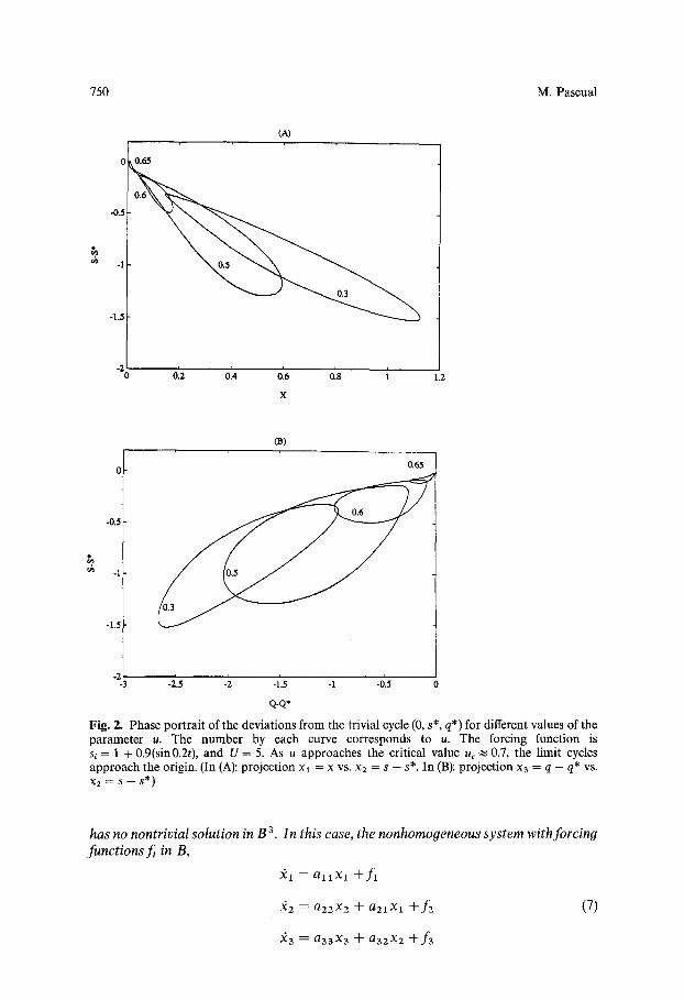
Theorems 2 and 3 show an exchange of local stability at u = uc similar to the one described for a constant nutrient forcing. Theorem 3 states the local stability of the positive periodic solution, both dynamically local in the sense of linearized stability and local near uc. It does not address the global stability of the solution. However, extensive simulation of (1) indicates that when u < u~, all positive trajectories converge to this cycle and, when u > u~, trajectories converge to the origin. Figure 2 shows some numerical results for a sinusoidal nutrient forcing. In this case, the simulations also confirm the critical value u¢, estimated here as falling between 0.65 and 0.7.
To prove Theorem 3, the following three lemmas are needed. The first one, due to Cushing (1977) and extended here to include one more variable, concerns the existence of periodic solutions for a particular 3-dimensional system with periodic coefficients. This lemma is used to write system (1) as an operator equation to which results from bifurcation theory apply. Lemma 2, a local bifurcation result due to Krasnosel'skii (1964), is then used to show that arbitrarily close to a trivial cycle, a periodic solution exists. Finally, this local result, valid for the bifurcation parameter arbitrarily close to a critical value, is extended to a larger region of parameter space by applying a global bifurcation result due to Rabinowitz (1971) and stated in Lemma 3.
A few lemmas:
Lemma 1 (Cushing 1977). Let aij ~ B, i, j = 1, 2, 3.
• (A) If(aii ) + O for i = 1, 2, 3, then the linear homogeneous system
Yl : allY1
Y2 = a 2 2 Y 2 + a21Yl (6)
3)3 = a33Y3 q- a 3 2 Y z
750 M. Pascual
(A)
0 ~ . . . .
i
-~ o'.2 oi~ A 0'.8 i X
1.2
0
-0.5
-1.5
fa)
0.65
i i
% -2.5 -2 -1.5 .'l -d.5 0 Q-Q*
Fig. 2. Phase por t ra i t of the devia t ions f rom the trivial cycle (0, s*, q*) for different values of the pa ramete r u. The n u m b e r by each curve cor responds to u. The forcing funct ion is si = 1 + 0.9(sin0.2t), and U = 5. As u approaches the critical value uc ~ 0.7, the l imit cycles a p p r o a c h the origin. (In (A): project ion x l = x vs. x2 = s - s*. In (B): project ion x3 = q - q* vs. X 2 ~ S -- S*)
has no nontrivial solution in B 3. In this case, the nonhomogeneous system with forcing functions fi in B,
Xi = aiixl nufi
2(2 = a22x2 -[- a21x1 + f 2 (7)
X3 = a33x3 "{- a32x2 + f 3

Phytoplankton response to nutrient fluctuations 751
has a unique solution (xi, x2, X3) in B 3. I f L denotes the operator from B 3 to itself, assigning to each set of forcing functions (f l , f2, f3) a solution (xl, xz, x3) of (7), then, L is linear and compact. Furthermore, if Li denotes the operator, from B to B, mapping the forcing function f to the solution of Yci = auxi + f then the operator L may be decomposed as
L (A, f2, fa) = (xl, x2, x3)
= ( L 1 A , L 2 ( a 2 1 L 1 A +f2), L3(a32L2(a21L~f1 +f2) +f3)) •
• (B) I f ( a l l ) = 0 and (a22) + 0 + (aaa 5, then (6) has exactly one independent solution in B 3.
In the next two lemmas G(2, x) denotes a one-parameter family of continuous compact operators from E = R x X to X, where X is a real Banach space. Furthermore, G = 2L(x) + H(2, x) with L linear and compact and H, o( II x Id) for x near 0 uniformly on bounded 2 intervals.
Lemma 2 (Krasnoset'skii 1964, Rabinowitz 1971). I f 2c is a characteristic value of L of odd multiplicity, then (2c, 0) is a bifurcation point of the equation G(2, x) = x with respect to the curve of trivial solutions.
Let f2 be an open set in E containing (2c, 0), and C be the set of nontrivial solutions of G(2, x) = x in E. The following lemma states a global bifurcation result for the case of non-globally defined operators H.
Lemma 3 (Rabinowitz 1971, Bardi 1984). Assume that 2c has multiplicity 1, and that H is defined on f2, H is independent of 2, and H is continuously (Frbchet) differentiable in a neighborhood of(2c, 0). Then, C contains two connected branches of solutions, meeting at (2o 0), and each satisfying one of the following alternatives. Each branch:
(i) is unbounded in E, or (ii) meets Of 2, the boundary of [2, or
(iii) meets (2, O) where 2 is a characteristic value of L, (2 + 2~).
Proof of Theorem 3. In the following proof of Theorem 3, a new real parameter 2 is introduced in (1) and chosen as a bifurcation parameter. A more natural choice would appear to be u. However, when (1) is written as an operator equation, its linear part L depends on u but not on 2, (see below). Thus, the application of the above lemmas is simplified by introducing 2 and considering the following system
S = u ( s i ( t ) - s ) - U x - - (8)
l + s
S 4 = - q + l + U
l + s
Note that (8) and (1) coincide for 2 = u. To prove Theorem 3, I will show that for 2 smaller than a critical value, including the desired case 2 = u when ( 1 - ~. - u) > 0, system (8) and therefore (1), has a nontrivial T-periodic solution.
752 M. Pascual
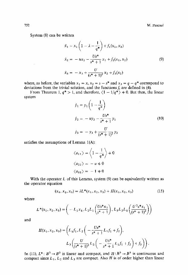
System (8) can be written
Us* X2 = -- ~/X2 - - X1 +f2 (x1 , X2)
s * + l (9)
U :~3 = - x 3 + ( s* + 1) ~ xz +f3(x~)
where, as before, the variables xl -- x, x2 = s - s* and x3 = q - q* correspond to deviations from the trivial solution, and the functions j~ are defined in (4).
From Theorem 1, q* > 1, and therefore, (1 - l / q * ) ~e 0. But then, the linear system
Us* Y2 = -- Hy2 S* + 1 Yl (10)
U ))3 = - Y3 + (s* + 1) ~ Y2
satisfies the assumptions of Lemma 1 (A):
(a11) = (1 - ~ , ) ~ 0
( a22 ) = - - u = # O
( a 3 3 ) = - 1 4 = 0
With the operator L of this Lemma, system (9) can be equivalently written as the operator equation
(xl, x2, x3) = 2L*(xl , x2, x3) + H(xl, xz, x3) (11)
where
and
L*(xl,xz, x3) = - -Llx l ,L2LI \s , + I j 'L3L2LI \ ~ i + ~ J ]
( ) H ( X l ' X 2 ' X 3 ) = L l f l ' L 2 s* +-----1Llfl + fz ,
L 3 ( i s , U Us* + f 2 ) + f 3 ) ) + ~ L 2 ( s, + l L l f l
In (11), L*: B 3 --*B 3 is linear and compact, and H:B 3 ---~B 3 is continuous and compact since L 1, L 2 and L 3 are compact. Also H is of order higher than linear

Phytoplankton response to nutrient fluctuations 753
near (0, 0, 0). Thus, Lemma 2 applies to (11), and bifurcation occurs at the non- trivial solutions of the linear equation (Yl, Y2, Y3)= 2L* (Yl, Y2, Y3), or equiv- alently, given the definition of L*, at the nontrivial solutions of
Us* ~ = - uy2 s* + 1 Yl (12)
U 3~3 = - Y3 + (s* + 1) ~ Y2 •
From Lemma I(A, B), (12) has a nontrivial solution in B 3 if and only if
13,
Since 2c can be shown to have multiplicity 1, (see Butler and Freedman 1981), bifurcation does in fact occur at this characteristic value. Then, (11) admits a continuum of nontrivial solutions in R × B 3, forming two branches that meet at (L, O, O, 0).
Near the bifurcation point, the set of nontrivial solutions is investigated with the following Lyapunov-Schmidt small parameter expansions,
2 = 2c + 21g + 22(g)g (14) X i ~- X i l e ~- Xi2 e2 ~- Xi3(t , e)e 2 (i = 1, 2, 3)
where e is a small parameter and ] 22(e)[ = 0([ el), I xi3(t, g)[o = O(I el)" Substituting these series in (9) (with the functions f~ written in expanded form) and equating coefficients of e and e 2, one obtains
Us* 221 = - - UX21 S* + 1 X l l (16)
U 231 = - - X31 ~- (S* 1 " ~ - ~ - ) X21 (17)
and
( q , ) 2 ) • (18)
Given an initial condition x 11 (0) > 0 , ( 1 5 ) implies that x 11 (t) = Xl 1 (0) e ~ o (1 - 2c - 1/q*)d~ is positive for all positive t. Then, from (16) and (17), both x21 and x31 are negative. Also, 21 must be negative, since x12 in (18) belongs to B if and only if 21 = (x31 / (q*) 2) (Halanay 1966 p. 226, or Lemma 2 in Cushing 1977). This lemma states that for a in B and (a ) = 0, the equation 2 = ax + f f e B , has a solution x ~ B if and only if ( f ( t ) e -S°a(s)as) = 0). It follows that arbitrarily close to the
754 M. Pascual
bifurcation point, the two branches of nontrivial solutions, denoted respectively by C~ + and C ( , satisfy
C + = {(2, x l , xz, x 3 ) ~ R x B 3 : 2 c - bo < 2 < 2c forsomebo ,x l > O, x2 < 0, x3 < 0 }
Ca- = {(2, x l , x 2 , x 3 ) s R x B 3 : 2 ~ < 2 < 2c + boforsomebo, x l < 0, x2 > 0, x3 > 0}
Let C2 + correspond to C ( when this set is defined with the variables x, s, q instead of x~, xz , x3. That is,
C2 + = {(2, x,s, q ) ~ R x B 3 : 2 ~ - bo < 2 < 2, for some bo, x > O, s < s*, q < q * } .
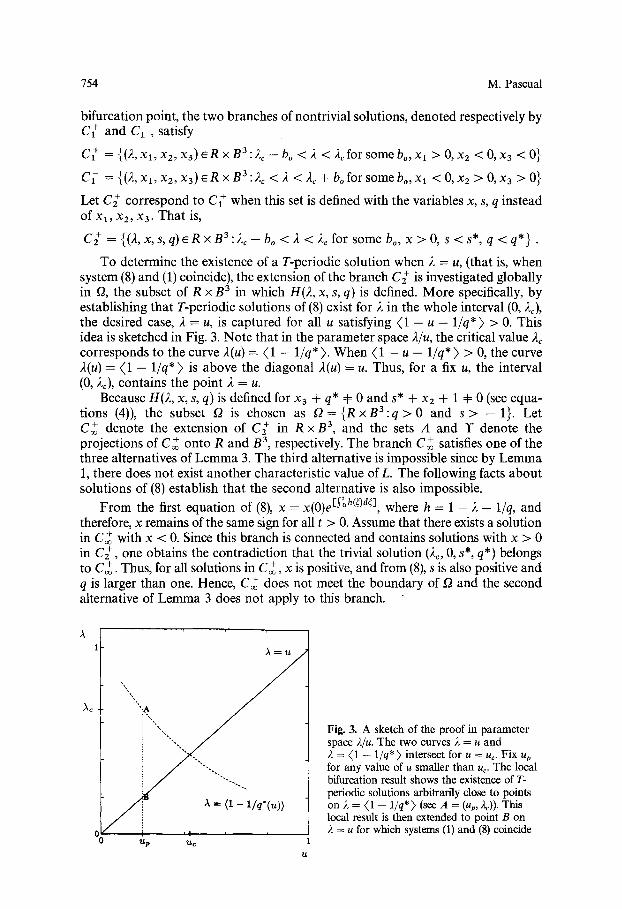
To determine the existence of a T-periodic solution when 2 = u, (that is, when system (8) and (1) coincide), the extension of the branch C ; is investigated globally in f2, the subset of R x B 3 in which H(2, x, s, q) is defined. More specifically, by establishing that T-periodic solutions of (8) exist for 2 in the whole interval (0, 2c), the desired case, 2 = u, is captured for all u satisfying (1 - u - l / q * ) > 0. This idea is sketched in Fig. 3. No te that in the parameter space 2/u, the critical value 2~ corresponds to the curve 2(u) = (1 - 1/q*) . When (1 - u - l / q * ) > 0, the curve 2(u) = (1 - l / q * ) is above the diagonal 2(u) = u. Thus, for a fix u, the interval (0, 2~), contains the point 2 = u.
Because H(2, x, s, q) is defined for x3 + q* 4= 0 and s* + xz + 1 4= 0 (see equa- tions (4)), the subset f2 is chosen as f2 = {R x B 3 : q > 0 and s > - 1 } . Let C + denote the extension of C~- in R >< B 3, and the sets A and Y denote the projections of C + onto R and B 3, respectively. The branch C + satisfies one of the three alternatives of L e m m a 3. The third alternative is impossible since by Lemma 1, there does no t exist another characteristic value of L. The following facts about solutions of (8) establish that the second alternative is also impossible.
~l(~'~[~h(Qd~] where h 1 2 - 1/q, and F r o m the first equation of (8), x = ~t,,1~ , = - therefore, x remains of the same sign for all t > 0. Assume that there exists a solution in C + with x < 0. Since this branch is connected and contains solutions with x > 0 in C2 + , one obtains the contradiction that the trivial solution (2c, 0, s*, q*) belongs to C + . Thus, for all solutions in C + , x is positive, and from (8), s is also positive and q is larger than one. Hence, C + does not meet the boundary of ~ and the second alternative of Lemma 3 does not apply to this branch.
1 t ", A = U
>,c
/ , ,, ~p Ue
Fig. 3. A sketch of the proof in parameter space 2/u. The two curves 2 = u and 2 = (1 - 1/q*) intersect for u = uc. Fix up for any value of u smaller than uc. The local bifurcation result shows the existence of T- periodic solutions arbitrarily close to points on 2 = (1 -- l/q*) (see A = (up, 2c)). This local result is then extended to point B on • ~ = u for which systems (1) and (8) coincide
Phytoplankton response to nutrient fluctuations 755
Finally, the first alternative of Lemma 3 must hold and either A or Y are unbounded (i.e. C + contains solutions with Ix ]o or [2] arbitrarily large). It is shown next that A is unbounded below and therefore contains the whole interval (0, 2c).
The set A is bounded above by 2~, (assuming otherwise implies that there exists solutions in C + with x < 0). Assume that A is bounded below. From (8), if h is Written as (h ) + Ah, then x( t ) = x(O)e<h)te ~°Ahd~. Since, e [S°Ahd~] belongs to B, then x belongs to B if and only if (h) = 0. In addition, since q > 1, there exists a constant M such that [hlo < M, for all solutions in C + . Thus, there exists constants N and P such that So Ahd~ < N and therefore ]XJo < P for all solutions in C + . But then, T is bounded, which contradicts Lemma 3. It follows that A must be unbounded below and therefore contains the whole interval (0, 2c). In particular, there exists a solution in C + for 2 = u. Thus, system (8), (or equivalently, system (1)), has a periodic solution in B 3. This completes the proof of the existence of a positive periodic solution.
To prove the local stability of this solution near u~ the proof of Theorem 8 in Cushing (1982) is closely followed. Local stability is demonstrated for 2 arbitrarily close to 2~. By applying this result to values of 2~ arbitrarily close to u~ (see Fig. 3), one obtains the desired local stability for u near uc.
Let N ( p ) denote and open ball in R x B 3 of radius p > 0 and center (2~, 0, 0, 0), and let C + denote the extension of C ( in R x B 3. The following arguments show that the solution (xl, x2, x3) of system (9) is locally asymptotically stable for (2, xl , x2, x3) E C + n N ( p ) - (2~, 0, 0, 0).
To determine the stability properties of the branch solution C + arbitrarily close to (2~, 0, 0, 0), system (9) is linearized at C +. This linearization yields,
x 3 + q * Yl + ( x 3 + q , ) 2 Y 3
X 1 S* -]- X 2 .92 = - - Uy2 - - U (S* -+" X 2 -+" 1) 2 22 - - U s * -[- x 2 + 1 Yl (19)
U ))3 = - - Y3 q- (S* q- X 2 -~- 1) 2 22
The local stability of the branch solution C + arbitrarily close to (2c, 0, 0, 0) is determined by the Floquet exponents of system (19). When the solution (2, Xl, x2, x3) is written with the small parameter expansions in (14), these Floquet exponents are also functions of the parameter e. Notice that for e = 0, system (19) becomes (12) (with 2 = 2c). Since (12) is a block triangular system, two of its Floquet exponents are those of the reduced system
.92 = - uy2 (20) U
/93= - - Y 3 + ( s . + I ) ~ y z
(Cushing 1982). Since (20) is locally asymptotically stable at (0, 0), these two Floquet exponents must have negative real parts. Thus, for e sufficiently small, two Floquet exponents of (19) must also have negative real parts. The remaining exponent of(12) is ((1 - 2c - ~.)) = 0. Thus, one needs to determine the location in the complex plane of the remaining exponent of (19) when e is small.

756 M. Pascual
But e is a Floquet exponent of (19) if and only if the system
~ = ( 1 - 2 1 ) X1 x 3 + q * e z l + ( x 3 + q , ) i z 3
X 1 S* ~- X 2 :~2= - - u z z - e z 2 - - U (s, + x2 + l) 2 z 2 - U s * + x 2 + l . z l (21)
U z 3 = - - z 3 - - e z 3 -l- (s* + x2 + 1) 2 Z2
has a nontrivial T-periodic solution for zi e B, (i = 1, 2, 3) (Cushing 1982). The sign of the real part of e is obtained by expanding e = ele + ez(e)~ and zi=zil(t)+z~z(t)e+zi3(t,e)~ where e is a small parameter and where [ex(~)l = O(l~l) and [zi3(t, e)[o = O(1~1). Substituting these series in (21) and equat- ing coefficients for the lowest order terms, one obtains equations for z~(t) equiva- lent to (15), (16) and (17) for xi~(t), (i = 1, 2, 3). Thus, Z~l(t) is positive for all t and both z2 l(t) and z31(t) are negative for all t. Equating coefficients for the first order
terms yields
z12 = (1 -- 2c -- ~ , ) z12 + ( -- 21 q
Then, zlz(t) belongs to B if and only if
( X 3__._.~ 1 __ -- 21 + (q , )2 el
X31 ) Xll (q*)2 el Zll -~ ( - ' - ~ Z31 •
Z31Xll ~ = 0 z l , (q , )2 /
(Lemma 2 in Cushing 1977), or equivalently,
/ Z31X11 ~ el = \ z l l ( q , ) 2 /
where the value of 21 has been used. Thus, el < 0 and e(e) < 0 for solutions in C+nN(p). It follows that solutions in C + n N ( p ) - (2c, 0,0, 0) are locally (uni- formly asymptotically) stable. For 2c arbitrarily close to u~, C + c~N(p) contains solutions of system (2) with ((1 - u - ~,)) > 0 (see Fig. 3). This completes the proof on the local stability of the T-periodic solution of system (1). []
Discussion
In spite of its nonlinearity, model (1) predicts a simple response of a phytoplankton population to the periodic supply of nutrients: an oscillation of exactly the same frequency as the forcings. The above results prove the existence and local, but not global, stability of this periodic solution. However, extensive simulation of the model indicates that positive trajectories converge to this cycle in the same region of parameter space where the trivial solution is known to be unstable. Also, the population response appears to mimic the temporal pattern of the nutrient inflow (Fig. 4).
This simple response of the model to a periodic nutrient supply may relate to its also simple behavior under constant forcing. In fact, the Droop equations under a constant supply of the resource present no oscillations in their approach to

Phytoplankton response to nutrient fluctuations 757
(A)
2
1.5
1
0.5
0 20
Si
TIME
1.2 03)
I
0.8
0.6
Si/l~
04 [ X 1////," ""'~"".. ,//"""
0.2 ,//"", ,, /'',,
% 50 60 70 8'0 90 100 110 120 130 140 TIME
Fig. 4. Numerical solutions for two different forcing functions. Curves for the nutrient inflow sl and the phytoplankton biomass x are shown. (si corresponds in (A) to the sine function
functxon ~k=l 1/(lO(t - 24k) 2 + 0.01)) 1 + 0.95 sin(0.4t), and in (B), to the pulse . k~5
equilibrium (Lange and Oyarzun 1992). Thus, the system lacks any internal frequency capable of interacting with external fluctuations to generate complex dynamics.
These results provide a basis to evaluate the model against experimental data in studies of phytoplankton population dynamics and nutrient variability. I am aware of a single such study by Olson and Chisholm (1983). Their data for H y m e n o m o n a s
c a r t e r a e grown under daily pulses of ammonium, reveals the expected presence of a 24 hour periodicity. However, a simple cycle with the same temporal pattern as the forcing may not be the whole story. After filtering and averaging the data,
7 5 8 M . P a s c u a l
Olson and Chisholm (1983) observe more than one single peak within 24 hours. More experiments are needed to provide longer data sets and cover a larger range of forcing frequencies.
Finally, two open questions related to this work are briefly mentioned. The first one concerns extending the results to general functions of uptake and growth. This generalization would include extensions of the Droop model that consider nutrient uptake a function of both the ambient and cellular nutrient levels (Rhee 1973). The second one regards a different approach to phytoplankton dynamics that views the population as distributed along the cell cycle. Since nutrient levels are known to affect progression of a phytoplankton cell through its cycle (Vaulot et al. 1987), this distribution may play an important role in the population response to nutrient fluctuations. This approach would consider the dynamics of both population biomass and cell numbers in fluctuating environments.
Models of the interplay between environmental variability and phytoplankton dynamics in continuous culture benefit from their powerful experimental setting. Their significance extends, however, to the broader context of oceanographic models that incorporate the nutrient-phytoplankton interaction. It is therefore essential that chemostat models capture the transfer of variability from the envi- ronment to the population.
Appendix
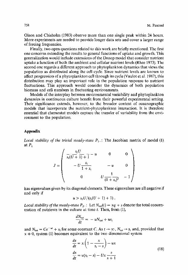
Local stability o f the trivial steady-state P1. : The Jacobian matrix of model (1) at P1
i siU si(U + 1) + I u 0 0 \
s i - - - - u 0 J= -UI+ &
1 0 U(1 s [ -~2+ ) 1
has eigenvalues given by its diagonal elements. These eigenvalues are all negative if and only if
u > s iU/(s i (U + 1) + 1).
Local stability o f the steady-state P2. : Let Ntot(t) = xq + s denote the total concen- tration of nutrients in the culture at time t. Then, from (1),
dNo, - - = - - u N t o t + usi
dt
and Ntot = Ce-ut + s~ for some constant C. As t ~ ~ , Ntot ~ sl and, provided that x =4 = 0, system (1) becomes equivalent to the two dimensional system
dt x 1 ux S i - -
(18) ds s d---[ = u(si - s) - Ux --s+l
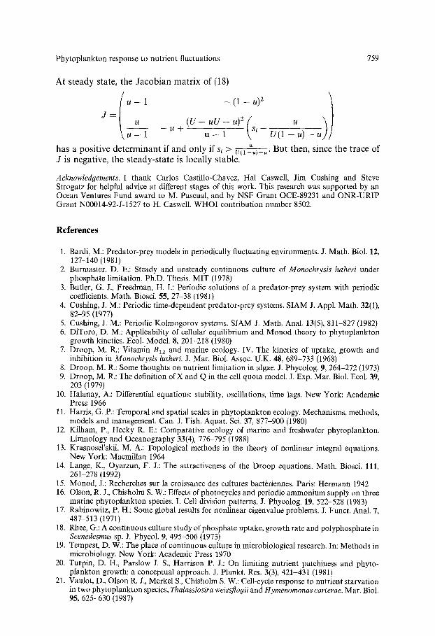
Phytoplankton response to nutrient fluctuations 759
At s teady state, the J acob ian mat r ix of (18)
u ( U - u g - u) 2 [ u
u -- 1 u + u - T T sl U(1 -S-u) -- u
has a posi t ive de t e rminan t if and only if si > v(1 ~u)-u. But then, since the t race of J is negative, the s teady-s ta te is local ly stable.
Acknowledgements. 1 thank Carlos Castillo-Chavez, Hal Caswell, Jim Cushing and Steve Strogatz for helpful advice at different stages of this work. This research was supported by an Ocean Ventures Fund award to M. Pascual, and by NSF Grant OCE-89231 and ONR-URIP Grant N00014-92-J-1527 to H. Caswell. WHOI contribution number 8502.
References
1. Bardi, M.: Predator-prey models in periodically fluctuating environments. J. Math. Biol. 12, 127-140 (1981)
2. Burmaster, D. E.: Steady and unsteady continuous culture of Monochrysis lutheri under phosphate limitation. Ph.D. Thesis. MIT (1978)
3. Butler, G. J., Freedman, H. I.: Periodic solutions of a predator-prey system with periodic coefficients. Math. Biosci. 55, 27-38 (1981)
4. Cushing, J. M.: Periodic time-dependent predator-prey systems. SIAM J. Appl. Math. 32(1), 82-95 (1977)
5. Cushing, J. M.: Periodic Kolmogorov systems. SIAM J. Math. Anal. 13(5), 811-827 (1982) 6. DiToro, D. M.: Applicability of cellular equilibrium and Monod theory to phytoplankton
growth kinetics. Ecol. Model. 8, 201-218 (1980) 7. Droop, M. R.: Vitamin Btz and marine ecology. IV. The kinetics of uptake, growth and
inhibition in Monochrysis lutheri. J. Mar. Biol. Assoc. U.K. 48, 689-733 (1968) 8. Droop, M. R.: Some thoughts on nutrient limitation in algae. J. Phycolog. 9, 264-272 (1973) 9. Droop, M. R.: The definition of X and Q in the cell quota model. J. Exp. Mar. Biol. Ecol. 39,
203 (1979) 10. Halanay, A.: Differential equations: stability, oscillations, time lags. New York: Academic
Press 1966 11. Harris, G. P.: Temporal and spatial scales in phytoplankton ecology. Mechanisms, methods,
models and management. Can. J. Fish. Aquat. Sci. 37, 877-900 (1980) 12. Kilham, P., Hecky R. E.: Comparative ecology of marine and freshwater phytoplankton.
Limnology and Oceanography 33(4), 776-795 (1988) 13. Krasnosel'skii, M. A.: Topological methods in the theory of nonlinear integral equations.
New York: Macmillan 1964 14. Lange, K., Oyarzun, F. J.: The attractiveness of the Droop equations. Math. Biosci. 111,
261-278 (1992) 15. Monod, J.: Recherches sur la croissance des cultures bact6riennes. Paris: Hermann 1942 16. Olson, R. J., Chisholm S. W.: Effects of photocycles and periodic ammonium supply on three
marine phytoplankton species. I. Cell division patterns. J. Phycolog. 19, 522-528 (1983) 17. Rabinowitz, P. H.: Some global results for nonlinear eigenvalue problems. J. Funct. Anal. 7,
487-513 (1971) 18. Rhee, G.: A continuous culture study of phosphate uptake, growth rate and polyphosphate in
Scenedesmus sp. J. Phycol. 9, 495-506 (1973) 19. Tempest, D. W.: The place of continuous culture in microbiological research. In: Methods in
microbiology. New York: Academic Press 1970 20. Turpin, D. H., Parslow J. S., Harrison P. J.: On limiting nutrient patchiness and phyto-
plankton growth: a conceptual approach. J. Plankt. Res. 3(3), 421-431 (1981) 21. Vaulot, D., Olson R. J., Merkel S., Chisholm S. W.: Cell-cycle response to nutrient starvation
in two phytoplankton species, Thalassiosira weissflogii and Hymenomonas carterae. Mar. Biol, 95, 625-630 (1987)