Well-posedness results for triply nonlinear degenerate parabolic equations
27
WELL-POSEDNESS RESULTS FOR TRIPLY NONLINEAR DEGENERATE PARABOLIC EQUATIONS B. ANDREIANOV, M. BENDAHMANE, K. H. KARLSEN, AND S. OUARO Abstract. We study the well-posedness of triply nonlinear degenerate elliptic- parabolic-hyperbolic problem b(u)t - div ˜ a(u, ∇φ(u)) + ψ(u)= f, u| t=0 = u 0 in a bounded domain with homogeneous Dirichlet boundary conditions. The nonlinearities b, φ and ψ are supposed to be continuous non-decreasing, and the nonlinearity ˜ a falls within the Leray-Lions framework. Some restrictions are imposed on the dependence of ˜ a(u, ∇φ(u)) on u and also on the set where φ de- generates. A model case is ˜ a(u, ∇φ(u)) = ˜ f(b(u),ψ(u),φ(u))+k(u)a 0 ( ∇φ(u)), with φ which is strictly increasing except on a locally finite number of seg- ments, and a 0 which is of the Leray-Lions kind. We are interested in existence, uniqueness and stability of entropy solutions. If b = Id, we obtain a general continuous dependence result on data u 0 ,f and nonlinearities b, ψ, φ, ˜ a. Simi- lar result is shown for the degenerate elliptic problem which corresponds to the case of b ≡ 0 and general non-decreasing surjective ψ. Existence, uniqueness and continuous dependence on data u 0 ,f are shown when [b + ψ](R)= R and φ ◦ [b + ψ] -1 is continuous. Date : October 13, 2008. 2000 Mathematics Subject Classification. Primary 35K65; Secondary 35A05. Key words and phrases. Degenerate hyperbolic-parabolic equation, conservation law, Leray- Lions type operator, non-Lipschitz flux, entropy solution, existence, uniqueness, stability. The work of K. H. Karlsen was supported by the Research Council of Norway through an Outstanding Young Investigators Award. The work of S. Ouaro was supported by the fundings from SARIMA, and then from the AUF. A part of this work was done while B. Andreianov and S. Ouaro enjoyed the hospitality of the Centre of Mathematics for Applications (CMA) at the University of Oslo, Norway. This article was written as part of the international research program on Nonlinear Partial Differential Equations at the Centre for Advanced Study at the Norwegian Academy of Science and Letters in Oslo during the academic year 2008–09. 1
Transcript of Well-posedness results for triply nonlinear degenerate parabolic equations
WELL-POSEDNESS RESULTS FOR TRIPLY NONLINEARDEGENERATE PARABOLIC EQUATIONS
B. ANDREIANOV, M. BENDAHMANE, K. H. KARLSEN, AND S. OUARO
Abstract. We study the well-posedness of triply nonlinear degenerate elliptic-
parabolic-hyperbolic problem
b(u)t − div a(u, ∇φ(u)) + ψ(u) = f, u|t=0 = u0
in a bounded domain with homogeneous Dirichlet boundary conditions. Thenonlinearities b, φ and ψ are supposed to be continuous non-decreasing, and the
nonlinearity a falls within the Leray-Lions framework. Some restrictions are
imposed on the dependence of a(u, ∇φ(u)) on u and also on the set where φ de-
generates. A model case is a(u, ∇φ(u)) = f(b(u), ψ(u), φ(u))+k(u)a0(∇φ(u)),
with φ which is strictly increasing except on a locally finite number of seg-ments, and a0 which is of the Leray-Lions kind. We are interested in existence,
uniqueness and stability of entropy solutions. If b = Id, we obtain a general
continuous dependence result on data u0, f and nonlinearities b, ψ, φ, a. Simi-lar result is shown for the degenerate elliptic problem which corresponds to the
case of b ≡ 0 and general non-decreasing surjective ψ. Existence, uniqueness
and continuous dependence on data u0, f are shown when [b+ψ](R) = R andφ [b+ ψ]−1 is continuous.
Date: October 13, 2008.
2000 Mathematics Subject Classification. Primary 35K65; Secondary 35A05.Key words and phrases. Degenerate hyperbolic-parabolic equation, conservation law, Leray-
Lions type operator, non-Lipschitz flux, entropy solution, existence, uniqueness, stability.The work of K. H. Karlsen was supported by the Research Council of Norway through an
Outstanding Young Investigators Award. The work of S. Ouaro was supported by the fundingsfrom SARIMA, and then from the AUF. A part of this work was done while B. Andreianov andS. Ouaro enjoyed the hospitality of the Centre of Mathematics for Applications (CMA) at the
University of Oslo, Norway. This article was written as part of the international research programon Nonlinear Partial Differential Equations at the Centre for Advanced Study at the NorwegianAcademy of Science and Letters in Oslo during the academic year 2008–09.
1
2 B. ANDREIANOV, M. BENDAHMANE, K. H. KARLSEN, AND S. OUARO
Contents
1. Introduction 21.1. Problem and assumptions 21.2. The notion of solution and known results 51.3. Main techniques and the outline of the paper 62. Entropy solutions and well-posedness results 72.1. Entropies and related notation 72.2. Entropy and entropy process solutions 72.3. Well-posedness of problem (P ) in the framework of entropy solutions. 93. Notation and preliminary lemmas 114. Proof of L1 contraction and comparison principles 145. A priori estimates 156. Proof of the general continuous dependence property 187. Proof of Theorem 2.3 238. Well-posedness for the doubly nonlinear elliptic problem 24References 26
1. Introduction
1.1. Problem and assumptions. In this paper we consider problems under thegeneral form
(P )
∂tb(u) + div f(b(u), ψ(u), φ(u))− div a(u, ∇φ(u)) + ψ(u) = f,
in QT = (0, T )× Ω,u|t=0 = u0 in Ω, u = 0 on (0, T )× ∂Ω,
where u : (t, x) ∈ QT −→ R is the unknown function, T > 0 is a fixed time,Ω ⊂ RN is a bounded domain with Lipschitz boundary ∂Ω.
We assume
(H1)∣∣∣∣ the functions b, ψ, φ : R 7→ R are continuous nondecreasing,
normalized by the value zero at the point zero.
We require the following technical assumption on φ:
(H2)∣∣∣ there exists a closed set E ⊂ R such that φ is strictly increasing on R \ E,
and the Lebesgue measure measφ(E) is zero;
and, moreover,
(H3) lim infε↓0 meas (Gε)/ε < +∞, where Gε := z ∈ R |dist (z, φ(E)) < ε.
Notice that since φ(·) is continuous and strictly monotone on R \ E, the set G :=φ(E) is also closed.
Remark 1.1. (i) Hypotheses (H2),(H3) are trivially satisfied if φ is a strictly in-creasing function. In case φ has a finite number of segments on which it keepsconstant values, E is just the union of all these “flatness segments”, and (H2),(H3)are satisfied.(ii) Property (H2) is still true if φ is locally absolutely continuous. In general,
WELL-POSEDNESS FOR DEGENERATE PARABOLIC EQUATIONS 3
the set of discontinuity points of φ−1 is not closed, and its closure can be large(this is the case, e.g., if φ is the “Cantor stairs function”). Thus (H2) is a re-striction, although it is fulfilled in most of the practical cases. Property (H3) is afurther restriction. Indeed, consider the following example. It is easy to constructa Lipschitz continuous non-decreasing function φ such that G = φ(E) is equal to0 ∪ 1/
√i | i ∈ N. A straightforward calculation shows that for ε = 1/n, Gε
contains the whole interval [0, 1/(2n2/3)]; in this case meas (Gε)/ε is of order ε−1/3
and gets unbounded as ε→ 0.
The initial function u0 : Ω → R and the source f : Q→ R are assumed to fulfill
(H4)
∣∣∣∣∣∣u0 ∈ L∞(Ω); f is measurable such that
f(t, ·) ∈ L∞(Ω) for a.e. t ∈ (0, T ) and∫ T
0
‖f(t, ·)‖L∞(Ω) dt < +∞.1
Furthermore, the following condition (automatically satisfied in the case b(R) = R)is needed :
(H5)
∣∣∣∣∣∣∣in the case b(+∞) 6= +∞ (resp., b(−∞) 6= −∞) one has
ψ(+∞) = +∞ and f+ ∈ L∞(QT )(resp., ψ(−∞) = −∞ and f− ∈ L∞(QT )
).
Assumptions (H4),(H5) are imposed to limit our study to bounded solutions of (P ).Note that in view of (H1) and (H5), we are assuming at least that (b+ψ)(R) = R.
An important part of the paper in devoted to the case b(R) = R. If, in addition,b is bijective, then performing a change of the unknown one puts the problem intothe doubly nonlinear framework with b = Id.
Our continuous dependence result for problem (P ) (in which we perturb boththe data and the nonlinearities) concerns the case where the structure condition
(Hstr) b(r) = b(s) ⇒ φ(r) = φ(s)
is satisfied. This result implies the existence of solutions for (P ), by reductionto non-degenerate problems. Assumption (Hstr) is trivially satisfied in the caseb = Id. If (Hstr) fails, the convergence of approximate solutions to (P ) is knownonly for a particular monotone approximation method developped by Ammar andWittbold [4]. This approach leads to an existence result which bypasses (Hstr);but interesting issues (such as proving convergence of numerical methods for (P )without requiring the structure condition (Hstr)) remain open. See Benilan andWittbold [14] for a thoroughful discussion of the role of the structure condition fora simple model one-dimensional case ∂tb(u) + (f(u))x = uxx.
Furthermore,
(H6) the function f : R×R×R → RN is assumed merely continuous.
Notice that under the structure condition (Hstr), the dependency of f on φ(u) cande dropped. Whenever it is convenient (and in particular, in the case where b isbijective), we use the notation f(·) := f(b(·), ψ(·), φ(·)).
The function a : R×RN → RN is assumed to satisfy the following conditions :
(H7) a is continuous2 on R×RN , and a(r, 0) ≡ 0;
1In the sequel, we will abusively denote the latter quantity by ‖f‖L1(0,T ;L∞(Ω)).
4 B. ANDREIANOV, M. BENDAHMANE, K. H. KARLSEN, AND S. OUARO
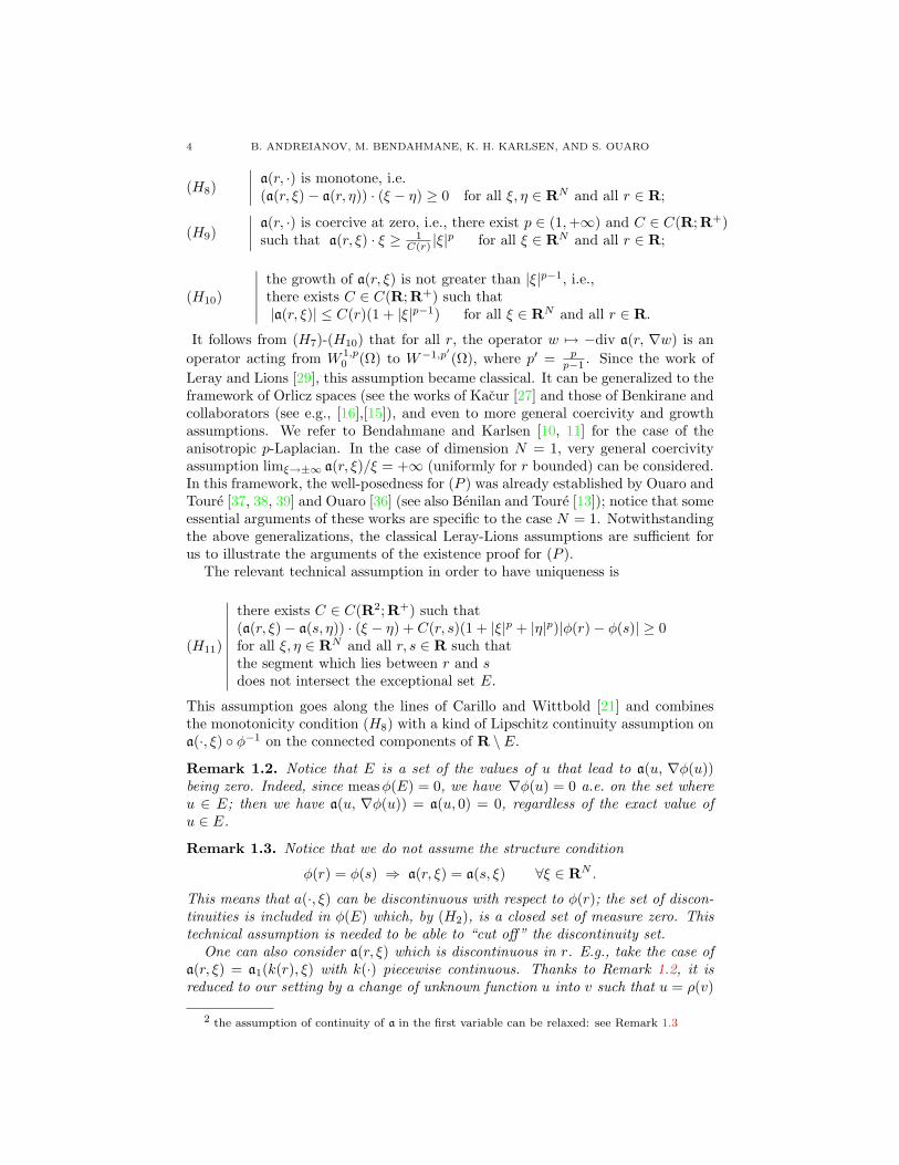
(H8)∣∣∣∣ a(r, ·) is monotone, i.e.
(a(r, ξ)− a(r, η)) · (ξ − η) ≥ 0 for all ξ, η ∈ RN and all r ∈ R;
(H9)∣∣∣∣ a(r, ·) is coercive at zero, i.e., there exist p ∈ (1,+∞) and C ∈ C(R;R+)
such that a(r, ξ) · ξ ≥ 1C(r) |ξ|
p for all ξ ∈ RN and all r ∈ R;
(H10)
∣∣∣∣∣∣the growth of a(r, ξ) is not greater than |ξ|p−1, i.e.,there exists C ∈ C(R;R+) such that|a(r, ξ)| ≤ C(r)(1 + |ξ|p−1) for all ξ ∈ RN and all r ∈ R.
It follows from (H7)-(H10) that for all r, the operator w 7→ −div a(r, ∇w) is anoperator acting from W 1,p
0 (Ω) to W−1,p′(Ω), where p′ = pp−1 . Since the work of
Leray and Lions [29], this assumption became classical. It can be generalized to theframework of Orlicz spaces (see the works of Kacur [27] and those of Benkirane andcollaborators (see e.g., [16],[15]), and even to more general coercivity and growthassumptions. We refer to Bendahmane and Karlsen [10, 11] for the case of theanisotropic p-Laplacian. In the case of dimension N = 1, very general coercivityassumption limξ→±∞ a(r, ξ)/ξ = +∞ (uniformly for r bounded) can be considered.In this framework, the well-posedness for (P ) was already established by Ouaro andToure [37, 38, 39] and Ouaro [36] (see also Benilan and Toure [13]); notice that someessential arguments of these works are specific to the case N = 1. Notwithstandingthe above generalizations, the classical Leray-Lions assumptions are sufficient forus to illustrate the arguments of the existence proof for (P ).
The relevant technical assumption in order to have uniqueness is
(H11)
∣∣∣∣∣∣∣∣∣∣there exists C ∈ C(R2;R+) such that(a(r, ξ)− a(s, η)) · (ξ − η) + C(r, s)(1 + |ξ|p + |η|p)|φ(r)− φ(s)| ≥ 0for all ξ, η ∈ RN and all r, s ∈ R such thatthe segment which lies between r and sdoes not intersect the exceptional set E.
This assumption goes along the lines of Carillo and Wittbold [21] and combinesthe monotonicity condition (H8) with a kind of Lipschitz continuity assumption ona(·, ξ) φ−1 on the connected components of R \ E.
Remark 1.2. Notice that E is a set of the values of u that lead to a(u, ∇φ(u))being zero. Indeed, since measφ(E) = 0, we have ∇φ(u) = 0 a.e. on the set whereu ∈ E; then we have a(u, ∇φ(u)) = a(u, 0) = 0, regardless of the exact value ofu ∈ E.
Remark 1.3. Notice that we do not assume the structure condition
φ(r) = φ(s) ⇒ a(r, ξ) = a(s, ξ) ∀ξ ∈ RN .
This means that a(·, ξ) can be discontinuous with respect to φ(r); the set of discon-tinuities is included in φ(E) which, by (H2), is a closed set of measure zero. Thistechnical assumption is needed to be able to “cut off” the discontinuity set.
One can also consider a(r, ξ) which is discontinuous in r. E.g., take the case ofa(r, ξ) = a1(k(r), ξ) with k(·) piecewise continuous. Thanks to Remark 1.2, it isreduced to our setting by a change of unknown function u into v such that u = ρ(v)
2 the assumption of continuity of a in the first variable can be relaxed: see Remark 1.3
WELL-POSEDNESS FOR DEGENERATE PARABOLIC EQUATIONS 5
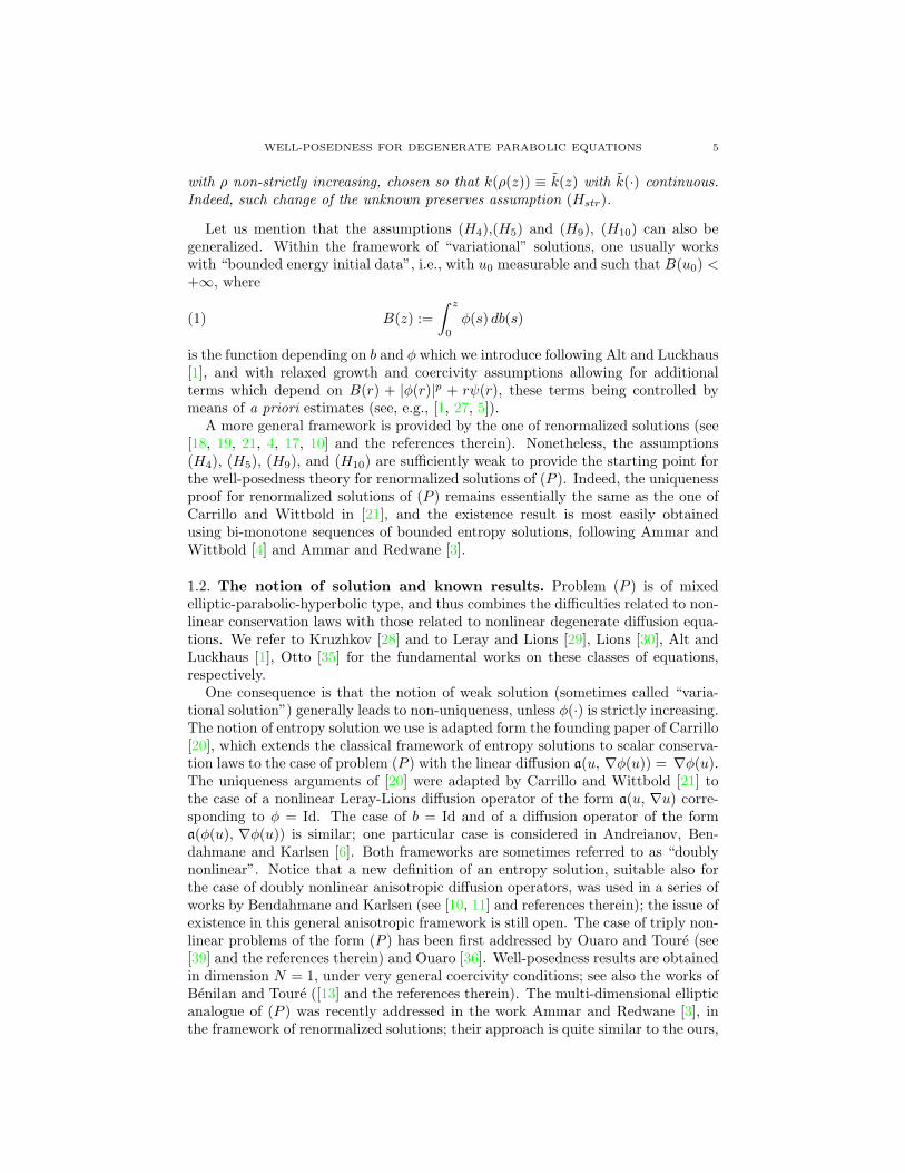
with ρ non-strictly increasing, chosen so that k(ρ(z)) ≡ k(z) with k(·) continuous.Indeed, such change of the unknown preserves assumption (Hstr).
Let us mention that the assumptions (H4),(H5) and (H9), (H10) can also begeneralized. Within the framework of “variational” solutions, one usually workswith “bounded energy initial data”, i.e., with u0 measurable and such that B(u0) <+∞, where
(1) B(z) :=∫ z
0
φ(s) db(s)
is the function depending on b and φ which we introduce following Alt and Luckhaus[1], and with relaxed growth and coercivity assumptions allowing for additionalterms which depend on B(r) + |φ(r)|p + rψ(r), these terms being controlled bymeans of a priori estimates (see, e.g., [1, 27, 5]).
A more general framework is provided by the one of renormalized solutions (see[18, 19, 21, 4, 17, 10] and the references therein). Nonetheless, the assumptions(H4), (H5), (H9), and (H10) are sufficiently weak to provide the starting point forthe well-posedness theory for renormalized solutions of (P ). Indeed, the uniquenessproof for renormalized solutions of (P ) remains essentially the same as the one ofCarrillo and Wittbold in [21], and the existence result is most easily obtainedusing bi-monotone sequences of bounded entropy solutions, following Ammar andWittbold [4] and Ammar and Redwane [3].
1.2. The notion of solution and known results. Problem (P ) is of mixedelliptic-parabolic-hyperbolic type, and thus combines the difficulties related to non-linear conservation laws with those related to nonlinear degenerate diffusion equa-tions. We refer to Kruzhkov [28] and to Leray and Lions [29], Lions [30], Alt andLuckhaus [1], Otto [35] for the fundamental works on these classes of equations,respectively.
One consequence is that the notion of weak solution (sometimes called “varia-tional solution”) generally leads to non-uniqueness, unless φ(·) is strictly increasing.The notion of entropy solution we use is adapted form the founding paper of Carrillo[20], which extends the classical framework of entropy solutions to scalar conserva-tion laws to the case of problem (P ) with the linear diffusion a(u, ∇φ(u)) = ∇φ(u).The uniqueness arguments of [20] were adapted by Carrillo and Wittbold [21] tothe case of a nonlinear Leray-Lions diffusion operator of the form a(u, ∇u) corre-sponding to φ = Id. The case of b = Id and of a diffusion operator of the forma(φ(u), ∇φ(u)) is similar; one particular case is considered in Andreianov, Ben-dahmane and Karlsen [6]. Both frameworks are sometimes referred to as “doublynonlinear”. Notice that a new definition of an entropy solution, suitable also forthe case of doubly nonlinear anisotropic diffusion operators, was used in a series ofworks by Bendahmane and Karlsen (see [10, 11] and references therein); the issue ofexistence in this general anisotropic framework is still open. The case of triply non-linear problems of the form (P ) has been first addressed by Ouaro and Toure (see[39] and the references therein) and Ouaro [36]. Well-posedness results are obtainedin dimension N = 1, under very general coercivity conditions; see also the works ofBenilan and Toure ([13] and the references therein). The multi-dimensional ellipticanalogue of (P ) was recently addressed in the work Ammar and Redwane [3], inthe framework of renormalized solutions; their approach is quite similar to the ours,

6 B. ANDREIANOV, M. BENDAHMANE, K. H. KARLSEN, AND S. OUARO
but the proofs of [3] require a special structure of the nonlinearity φ. We bypassthe difficulties of [3] using two observations in Section 3 (see Lemmas 3.2,3.3).
In most of the works cited hereabove, the homogeneous Dirichlet boundary con-ditions were chosen. One should bear in mind that, unless φ is strictly increasing,the boundary condition is also understood in an entropy sense (see e.g. Bardos,LeRoux and Nedelec [9], Otto [34], Carrillo [20]). Focusing on the homogeneousboundary condition is a simplification which seems to be not merely technical. Apartial extension of the Carrillo’s techniques to inhomogeneous boundary data canbe found in Ammar, Carrillo and Wittbold [2]. Different techniques for the inho-mogeneous problem, based on the weak trace framework introduced by Otto [34]and developed by Chen and Frid [22], were used by Mascia, Porretta and Terracina[32] and Michel and Vovelle [33]. A related, though somewhat more straightforwardapproach was attempted by Andreianov and Igbida [7]. Notice that in all cases, atechnique of “going up to the boundary” is preceded by obtaining the fundamentalweak formulations and entropy inequalities “inside the domain”. In the presentpaper, we also make the simplest choice of the homogeneous Dirichlet data, andfocus on deriving the entropy inequalities.
1.3. Main techniques and the outline of the paper. Our main concern isthe existence for (P ) (and more generally, the continuous dependence result withrespect to perturbations of the data and the nonlinearities) in the case b = Id(or, more generally, under the structure condition (Hstr)). We extend the ar-guments of Andreianov, Bendahmane and Karlsen [6] developed for the case ofa(u, ∇φ(u)) ≡ a(∇φ(u)); the main difficulty stems from the fact that we do notassume the structure condition of Remark 1.3, so that a(φ−1(·), ξ) can be discon-tinuous.
In order to use the weak convergence while passing to the limit in the nonlineardiffusion term in (P ), we use a version of the classical Minty-Browder monotonicityargument. We use cut-off functions to focalize on the intervals of the strict mono-tonicity of φ. We then show that the complementary of this set can be neglected,thanks to a particular a priori estimate with the cut-off function which localizes ona neigbourhood of the “exceptional set” E of the values of u introduced in (H2)(see Remark 1.2 and Lemma 3.2).
In order to deal with the convection term in (P ), we use the technique of non-linear weak-∗ convergence to a measure-valued solution (as considered by Tartar,DiPerna, Szepessy, Panov), or more exactly, to an entropy process solution as de-veloped by Gallouet and collaborators (see [25, 23, 24] and references therein).Considering entropy process solutions is a purely technical issue, since the unique-ness proof also contains their identification to entropy solutions.
The chain rule arguments of Lemmas 3.3,3.4 permit to separate the two afore-mentioned weak convergence arguments, the one for the diffusion term and the onefor the convection term.
The uniqueness of an entropy solution is shown under the assumption (H11), withthe help of (H3) and the estimate of Lemma 3.2; we follow Carrillo [20], Carrilloand Wittbold [21], Eymard, Gallouet, Herbin and Michel [24] and Andreianov,Bendahmane and Karlsen [6].
WELL-POSEDNESS FOR DEGENERATE PARABOLIC EQUATIONS 7
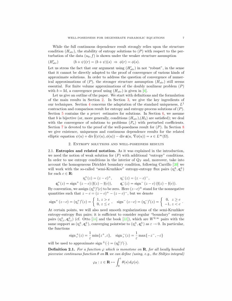
While the full continuous dependence result strongly relies upon the structurecondition (Hstr), the stability of entropy solutions to (P ) with respect to the per-turbation of the data (u0, f) is shown under the weaker structure assumption
(H ′str) (b+ ψ)(r) = (b+ ψ)(s) ⇒ φ(r) = φ(s).
Let us stress the fact that our argument using (H ′str) in not “robust”, in the sense
that it cannot be directly adapted to the proof of convergence of various kinds ofapproximate solutions. In order to address the question of convergence of numer-ical approximations of (P ), the stronger structure assumption (Hstr) still seemsessential. For finite volume approximations of the doubly nonlinear problem (P )with b = Id, a convergence proof using (Hstr) is given in [6].
Let us give an outline of the paper. We start with definitions and the formulationof the main results in Section 2. In Section 3, we give the key ingredients ofour techniques. Section 4 concerns the adaptation of the standard uniqueness, L1
contraction and comparison result for entropy and entropy-process solutions of (P ).Section 5 contains the a priori estimates for solutions. In Section 6, we assumethat b is bijective (or, more generally, conditions (Hstr),(H5) are satisfied); we dealwith the convergence of solutions to problems (Pn) with perturbed coefficients.Section 7 is devoted to the proof of the well-posedness result for (P ). In Section 8we give existence, uniqueness and continuous dependence results for the relatedelliptic equation ψ(u) + div f(ψ(u), φ(u))− div a(u, ∇φ(u)) = s ∈ L∞(Ω).
2. Entropy solutions and well-posedness results
2.1. Entropies and related notation. As it was explained in the introduction,we need the notion of weak solution for (P ) with additional “entropy” conditions.In order to use entropy conditions in the interior of QT and, moreover, take intoaccount the homogeneous Dirichlet boundary condition, following Carrillo [20] wewill work with the so-called “semi-Kruzhkov” entropy-entropy flux pairs (η±c , q
±c )
for each c ∈ R:η+
c (z) = (z − c)+, η−c (z) = (z − c)−,q+
c (z) = sign+ (z − c) (f(z)− f(c)), q−c (z) = sign− (z − c) (f(z)− f(c)).By convention, we assign (η±c )′(c) to be zero. Here (z−c)± stand for the nonnegativequantities such that z − c = (z − c)+ − (z − c)−, but we denote
sign+ (z−c) = (η+c )′(z) =
1, z > c0, z ≤ c
, sign− (z−c) = (η−c )′(z) =
0, z ≥ c−1, z < c
.
At certain points, we will also need smooth regularizations of the semi-Kruzhkoventropy-entropy flux pairs; it is sufficient to consider regular “boundary” entropypairs (η±c,ε, q
±c,ε) (cf. Otto [34] and the book [31]), which are W 2,∞ pairs with the
same support as (η±c , q±c ), converging pointwise to (η±c , q
±c ) as ε→ 0. In particular,
the functions
sign +ε (z) =
1ε
minz+, ε, sign−ε (z) =1ε
max−z−,−ε
will be used to approximate sign±(·) = (η±0 )′(·).Definition 2.1. For a function ϕ which is monotone on R, for all locally boundedpiecewise continuous function θ on R we can define (using, e.g., the Stiltjes integral)
ϕθ : z ∈ R 7→∫ z
0
θ(s) dϕ(s).

8 B. ANDREIANOV, M. BENDAHMANE, K. H. KARLSEN, AND S. OUARO
Moreover (see Lemma 3.1 below), there exists a continuous function ϕθ such thatϕθ(u) = ϕθ(ϕ(u)).
In the sequel, we denote by b±c (·) the function z 7→∫ z
0
(η±c )′(s) db(s).
2.2. Entropy and entropy process solutions. For the sake of simplicity, we willin this paper work with bounded entropy solutions, i.e., we require that u ∈ L∞(QT )and put corresponding hypotheses on the data u0, f and functions b, ψ. Note thatthe boundedness assumption can be bypassed in the framework of renormalizedsolutions (see in particular Ammar and Redwane [3]); or in the framework of varia-tional solutions in the spirit of Alt and Luckhaus [1] (in this case, one has to replacethe functions C(·) in assumptions (H9), (H10), (H11) with a constant C; furtherchanges are indicated in Remark 6.1).
Definition 2.2 (entropy solution). An entropy solution of (P ) is a measurablefunction u : QT → R satisfying the following conditions:(D.1) (regularity) u ∈ L∞(QT ) and w = φ(u) ∈ Lp(0, T ;W 1,p
0 (Ω)).
(D.2) For all ξ ∈ D([0, T )× Ω),∫ ∫QT
(b(u)∂tξ + f(u) · ∇ξ − a(u,∇w) · ∇ξ − ψ(u)ξ
)dx dt
+∫
Ω
b(u0)ξ(0, ·) dx+∫ ∫
QT
fξ dxdt = 0.(2)
(D.3) For all (c, ξ) ∈ R± × D([0, T ) × Ω), ξ ≥ 0, and also for all (c, ξ) ∈ R ×D([0, T )× Ω), ξ ≥ 0,∫ ∫
QT
(b±c (u)∂tξ + q±c (u) · ∇ξ − (η±c )′(u)a(u,∇w) · ∇ξ − (η±c )′(u)ψ(u)ξ
)dx dt
+∫
Ω
b±c (u0)ξ(0, ·) dx+∫ ∫
QT
(η±c )′(u) fξ dxdt ≥ 0.
Remark 2.1. If in the above definition, u satisfies (D.1), if (2) is replaced bythe inequality “≥” (resp., with the inequality “≤”), and if (D.3) holds with theentropies η+
c for c ∈ R+ (resp., with the entropies η−c for c ∈ R−), then u is calledentropy subsolution (resp., entropy supersolution) of (P ).
Remark 2.2. Following Alt and Luckhaus [1], we can rewrite the weak formulation(2) of (P ) as follows:- b(u)|t=0 = b(u0) and the distributional derivative ∂tb(u) satisfies
∂tb(u) ∈ Lp′(0, T ;W−1,p′(Ω)) + L1(QT )
in the sense ∫ T
0
〈∂tb(u) , ζ〉 = −∫ ∫
QT
b(u) ∂tζ −∫
Ω
b(u0)ζ(0, ·)
for all ζ ∈ Lp(0, T,W 1,p0 (Ω)) ∩ L∞(QT ) such that ∂tζ ∈ L∞(QT ) and ζ(T, ·) = 0;
- equation (P ) is satisfied in Lp′(0, T ;W−1,p′(Ω)) + L1(QT ).
We denote by 〈 · , · 〉 the duality pairing between Lp′(0, T ;W−1,p′(Ω))+L1(QT ) andLp(0, T,W 1,p
0 (Ω)) ∩ L∞(QT ).

WELL-POSEDNESS FOR DEGENERATE PARABOLIC EQUATIONS 9
For technical reasons, it is convenient to introduce the notion of entropy pro-cess solution adapted from Eymard, Gallouet and Herbin [23], Gallouet and Hu-bert [25] and Eymard, Gallouet, Herbin and Michel [24]. This definition is basedupon the so-called “nonlinear weak-? convergence” property (see e.g., Ball [8] andHungerbuhler [26]):
(3)
∣∣∣∣∣∣∣∣∣∣each sequence (un)n of measurable functionsadmits a subsequence such that for all F ∈ C(R,R),
F (un(·)) →∫ 1
0
F (µ(·, α)) dα weakly in L1(QT )
whenever the set (F (un))n is weakly relatively compact in L1(QT ),
where the function µ ∈ L∞(QT × (0, 1)) is referred to as the “process function”.Notice that in the above statement, one also concludes that F (µ(·, α)) independentof α whenever F (un) converges to F (u) in measure (see Hungerbuhler [26]).
Definition 2.3 (entropy process solution). An entropy process solution of (P ) isa couple (µ,w) of measurable functions µ : QT × (0, 1) → R and w : QT → Rsatisfying the following conditions:
(D’.1) (regularity and consistency) µ ∈ L∞(QT × (0, 1)), w ∈ Lp(0, T ;W 1,p0 (Ω)),
and φ(µ(t, x, α)) ≡ w(t, x) for a.e. (t, x, α) ∈ QT × (0, 1).
(D’.2) For all ξ ∈ D([0, T )× Ω),∫ 1
0
∫ ∫QT
(b(µ)∂tξ + f(µ) · ∇ξ − a(µ, ∇w) · ∇ξ − ψ(µ)ξ
)dx dtdα
+∫
Ω
u0ξ(0, ·) dx+∫ ∫
QT
fξ dxdt = 0.
(D’.3) For all (c, ξ) ∈ R± × D([0, T ) × Ω), ξ ≥ 0, and also for all (c, ξ) ∈ R ×D([0, T )× Ω), ξ ≥ 0,∫ 1
0
∫ ∫QT
(b±c (µ)∂tξ + q±c (µ) · ∇ξ − (η±c )′(µ)a(µ,∇w) · ∇ξ − (η±c )′(µ)ψ(µ)
)dx dtdα
+∫
Ω
b±c (u0)ξ(0, ·) dx+∫ 1
0
∫ ∫QT
(η±c )′(µ) fξ dxdtdα ≥ 0.
Remark 2.3. In (D’.3), setting u :=∫ 1
0
µ(α) dα one can rewrite the third term
under the form∫ 1
0
∫ ∫QT
(η±c )′(µ)a(µ,∇w) =∫ ∫
QT
(η±c )′(u)a(u, ∇w).
Indeed, we have w ≡ φ(µ), and φ is invertible on R \ E, so that µ(t, x, α) ≡φ−1(w(t, x)) = u(t, x) whenever w(t, x) ∈ R \ φ(E); furthermore, ∇w = 0 a.e. on[w ∈ φ(E) ∪ φ(c) ], and the exact value of (η±c )′(µ) on [w ∈ φ(E) ∪ φ(c) ] doesnot matter because a(r, 0) ≡ 0. For the same reasons, a(µ,∇w) can be replaced bya(u,∇w) in (D’.2).

10 B. ANDREIANOV, M. BENDAHMANE, K. H. KARLSEN, AND S. OUARO
Remark 2.4. If u is an entropy solution of (P ), then the couple (µ,w) defineda.e. on QT × (0, 1) (resp., on QT ) by µ(t, x, α) = u(t, x) (resp., by w(t, x) =φ(u(t, x))), is an entropy process solution of (P ). In turn, if (µ,w) is an entropyprocess solution of (P ) such that µ(t, x, α) = u(t, x) a.e. on QT × (0, 1) for someu : QT −→ R, then the function u is an entropy solution of (P ).
2.3. Well-posedness of problem (P ) in the framework of entropy solutions.First note the uniqueness result, which requires no range condition nor structurecondition on the nonlinearities b and φ.
Theorem 2.1. Assume that (H1)-(H5) and (H6)-(H11) hold.(i) Assume that (µ,w) is an entropy process solution of (P ). Then
u(t, x) =∫ 1
0
µ(t, x, α) dα
is an entropy solution of (P ). Moreover, we have b(µ)(t, x, α) ≡ b(u)(t, x) andψ(µ)(t, x, α) ≡ ψ(u)(t, x) a.e. on QT × (0, 1). If (b + φ + ψ) is strictly increasing,then µ(t, x, α) = u(t, x) a.e. on QT × (0, 1).(ii) Assume that u and u are two entropy solutions of (P ) corresponding to the datau0, f and u0, f , respectively. Then for a.e. t ∈ (0, T ),∫
Ω
(b(u)− b(u))+(t) +∫ t
0
∫Ω
(ψ(u)− ψ(u))+
≤∫
Ω
(b(u0)− b(u0))+ +∫ t
0
∫Ω
sign +(u− u)(f − f).
(iii) In particular, if u, u are two entropy solutions of (P ), then b(u) ≡ b(u) andψ(u) ≡ ψ(u).
Remark 2.5. In Theorem 2.1(ii), on can replace u, resp. u, with an entropysubsolution, resp. with an entropy super-solution. The same proof applies.
The following continuous dependence property is the central result of this paper.
Theorem 2.2. Let (bn, ψn, φn, an, fn;un0 , fn), n ∈ N, be a sequence converging to
(b, ψ, φ, a, f;u0, f) in the following sense:
(4)· bn, ψn, φn converge pointwise to b, ψ, φ respectively;· fn, an converge to f, a, respectively, uniformly on compacts;· bn(un
0 ) → b(u0) in L1(Ω), and fn → f in L1(QT ).
Assume that (b, ψ, φ, a, f;u0, f) and (bn, ψn, φn, an, fn;un0 , fn) (for each n) satisfy the
hypotheses (H1), (H4), (H5), and (H6)-(H11), and, moreover, that the functionsC(·) in (H9), (H10), and (H11) as well as the L∞(Ω) and L1(0, T, L∞(Ω)) boundsin (H4) are independent of n. We denote by (Pn) the analogue of problem (P )corresponding to the data and coefficients (bn, ψn, φn, an, fn;un
0 , fn).Assume that either b(R) = R, or the L∞(QT ) bounds on f±n in (H5) are inde-
pendent of n. Assume that the structure condition (Hstr) holds, and φ satisfies thetechnical hypotheses (H2),(H3).
Let un be an entropy solution of problem (Pn). Then the functions un convergeto an entropy solution u of (P ) in L∞(QT ) weakly-*, up to a subsequence. Further-more, the functions φn(un) converge to φ(u) in L1(QT ) up to a subsequence, andthe whole sequences bn(un), ψn(un) converge in L1(QT ) to b(u), ψ(u), respectively.
WELL-POSEDNESS FOR DEGENERATE PARABOLIC EQUATIONS 11
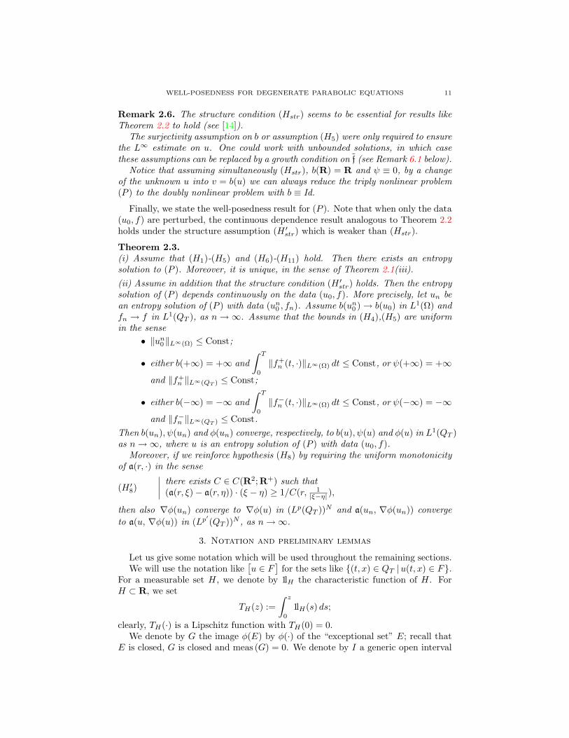
Remark 2.6. The structure condition (Hstr) seems to be essential for results likeTheorem 2.2 to hold (see [14]).
The surjectivity assumption on b or assumption (H5) were only required to ensurethe L∞ estimate on u. One could work with unbounded solutions, in which casethese assumptions can be replaced by a growth condition on f (see Remark 6.1 below).
Notice that assuming simultaneously (Hstr), b(R) = R and ψ ≡ 0, by a changeof the unknown u into v = b(u) we can always reduce the triply nonlinear problem(P ) to the doubly nonlinear problem with b ≡ Id.
Finally, we state the well-posedness result for (P ). Note that when only the data(u0, f) are perturbed, the continuous dependence result analogous to Theorem 2.2holds under the structure assumption (H ′
str) which is weaker than (Hstr).
Theorem 2.3.(i) Assume that (H1)-(H5) and (H6)-(H11) hold. Then there exists an entropysolution to (P ). Moreover, it is unique, in the sense of Theorem 2.1(iii).(ii) Assume in addition that the structure condition (H ′
str) holds. Then the entropysolution of (P ) depends continuously on the data (u0, f). More precisely, let un bean entropy solution of (P ) with data (un
0 , fn). Assume b(un0 ) → b(u0) in L1(Ω) and
fn → f in L1(QT ), as n→∞. Assume that the bounds in (H4),(H5) are uniformin the sense
• ‖un0‖L∞(Ω) ≤ Const;
• either b(+∞) = +∞ and∫ T
0
‖f+n (t, ·)‖L∞(Ω) dt ≤ Const, or ψ(+∞) = +∞
and ‖f+n ‖L∞(QT ) ≤ Const;
• either b(−∞) = −∞ and∫ T
0
‖f−n (t, ·)‖L∞(Ω) dt ≤ Const, or ψ(−∞) = −∞
and ‖f−n ‖L∞(QT ) ≤ Const.Then b(un), ψ(un) and φ(un) converge, respectively, to b(u), ψ(u) and φ(u) in L1(QT )as n→∞, where u is an entropy solution of (P ) with data (u0, f).
Moreover, if we reinforce hypothesis (H8) by requiring the uniform monotonicityof a(r, ·) in the sense
(H ′8)
∣∣∣∣ there exists C ∈ C(R2;R+) such that(a(r, ξ)− a(r, η)) · (ξ − η) ≥ 1/C(r, 1
|ξ−η| ),
then also ∇φ(un) converge to ∇φ(u) in (Lp(QT ))N and a(un, ∇φ(un)) convergeto a(u, ∇φ(u)) in (Lp′(QT ))N , as n→∞.
3. Notation and preliminary lemmas
Let us give some notation which will be used throughout the remaining sections.We will use the notation like
[u ∈ F
]for the sets like (t, x) ∈ QT |u(t, x) ∈ F.
For a measurable set H, we denote by 1lH the characteristic function of H. ForH ⊂ R, we set
TH(z) :=∫ z
0
1lH(s) ds;
clearly, TH(·) is a Lipschitz function with TH(0) = 0.We denote by G the image φ(E) by φ(·) of the “exceptional set” E; recall that
E is closed, G is closed and meas (G) = 0. We denote by I a generic open interval
12 B. ANDREIANOV, M. BENDAHMANE, K. H. KARLSEN, AND S. OUARO
in R \E, and by J it image φ(I) which is a generic open interval in R \G. For allε > 0, we choose an open set Gε ⊃ G such that meas (Gε) < Const× ε. We denoteby Eε the open set φ−1(Gε) which contains E. When (H3) holds, we can simplytake Gε = Gε := z ∈ R |dist (z,G) < ε.
Now let us prove the representation property used in Definition 2.1.
Lemma 3.1. Let ϕθ(·) be the function defined by
ϕθ : z ∈ R 7→∫ z
0
θ(s) dϕ(s),
for a continuous non-decreasing function ϕ : R → R and a bounded piecewisecontinuous function θ : R → Rn. Then there exists a Lipschitz continuous functionϕθ : ϕ(R) → Rn such that for all z ∈ R,
ϕθ(z) = ϕθ(ϕ(z)).
Proof. If ϕ(z) = ϕ(z), then the measure dϕ(s) vanishes between z and z; thus
ϕθ(z) − ϕθ(z) =∫ z
z
θ(s) dϕ(s) is zero. Therefore ϕθ is well defined. For all r, r ∈
ϕ(R), ϕθ(r) − ϕθ(r) = ϕθ(z) − ϕθ(z) =∫ z
z
θ(s) dϕ(s), where z ∈ ϕ−1(r), z ∈
ϕ−1(r). Thus
|ϕθ(r)− ϕθ(r)| ≤ ‖θ‖L∞ |ϕ(z)− ϕ(z)| = ‖θ‖L∞ |r − r|.
Now, let us give a localized estimate of the gradient of w = φ(u).
Lemma 3.2. Let u be a bounded weak solution of (P ). Then there exists a constantC depending on C(·) in (H9), on ‖u‖L∞(QT ) and on ‖b(u0)‖L1(Ω), ‖f‖L1(Q) suchthat for all Borel measurable set F ⊂ R,
IF (u) :=∫ ∫[
u∈F] |∇φ(u)|p =
∫ ∫[w∈φ(F )
] |∇w|p≤ C VarFφ(·) = Cmeas (φ(F )).
(5)
Proof. Without loss of restriction, one can assume that F is bounded; indeed,otherwise we can replace F with FM := F ∩ [−M,M ] and then pass to the limitas M → +∞ in inequality (5) written for FM .
Set H = φ(F ), and note that TH(w) = TH(φ(u)) ∈ Lp(0, T ;W 1,p0 (Ω)) can be
approximated by admissible test functions in (2) of Definition 2.2; one has
∇TH(w) = ∇w1lH(w) = ∇φ(u)1lF (u),
and
(6) ‖TH(·)‖∞ ≤∫
F
dφ(s) = VarFφ(·) = meas (H).
Using this test function, with Remark 2.2 and the standard chain rule argumentknown as the Mignot-Bamberger and Alt-Luckhaus formula (see, e.g., Alt andLuckhaus [1], Otto [35], Carrillo and Wittbold [21]) we get
(7)
∫Ω
BF (u)(T, ·) +∫ ∫
QT
ψ(u)TH(φ(u)) +∫ ∫
QT
a(u, ∇w) · ∇TH(w)
=∫
Ω
BF (u0) +∫ ∫
QT
fTH(w)−∫ ∫
QT
f(u) · ∇TH(φ(u)),
WELL-POSEDNESS FOR DEGENERATE PARABOLIC EQUATIONS 13
where BF (z) =∫ z
0
TH(φ(s)) db(s). The last term is zero thanks to the boundary
condition w|Σ = 0. Indeed, because F is assumed bounded, f(·) is bounded onthe support of T ′H(φ(·)); thus by Lemma 3.1 there exists a Lipschitz continuousvector-valued function g(·) such that∫ z
0
f(s) dTH(φ(s)) = g(φ(z)).
Hence g w ∈ Lp(0, T ;W 1,p0 (Ω;RN )), so that one can apply the Green-Gauss
formula to get ∫ ∫Q
div(∫ w
0
f(s) dTH(φ(s)))
=∫ T
0
∫∂Ω
g(w) · ν = 0,
where ν is the exterior unit normal vector to ∂Ω. By definition of TH(·) and becauseφ(·) is non-decreasing, dropping positive terms in the left-hand side of (7), by (H9)we infer
1C(‖u‖L∞(QT ))
∫ ∫[u∈F ]
∣∣∇φ(u)∣∣p ≤ ∫ ∫
[w∈φ(F )]
a(u, ∇w) · ∇w
≤(‖b(u0)‖L1(Ω) + ‖f‖L1(Q)
)‖TH(·)‖∞.
Hence the claim follows by (6).
In the above proof, we have used two chain rule lemmas. Now we notice thatboth apply for u(·) replaced with a “process function” µ(·, α), as in (D’.1), providedthat for a.e. α ∈ (0, 1) one can substitute
u(t, x) :=∫ 1
0
µ(t, x, α) dα
by µ(t, x, α) in the expression of the test function.
Lemma 3.3. Let (µ,w) satisfy (D’.1), and S : R → R be a Lipschitz continuousfunction such that S(0) = 0. Let ζ ∈ L∞(0, T ). Then∫ ∫
QT
∫ 1
0
f(µ(t, x, α))) · ∇S(w(t, x)) ζ(t) dtdxdα = 0.
Proof. By Lemma 3.1, there exists a Lipschitz vector-valued function g such that∫ z
0
f(s) dS(φ(s)) = g(φ(z)) for |z| ≤ ‖µ‖L∞(QT×(0,1)). We have∫ ∫QT
∫ 1
0
f(µ(α)) dα · ∇S(φ(u)) ζ
=∫ ∫
QT
∫ 1
0
f(µ(α)) · ∇S(φ(µ(α))) dα ζ
=∫ ∫
QT
∫ 1
0
div(∫ µ(α)
0
f(s) dS(φ(s)))dα ζ
=∫ T
0
∫Ω
div g(w) ζ =∫ T
0
∫∂Ω
g(w) · ν ζ = 0
because for a.e. α ∈ (0, 1), φ(µ(α)) ≡ φ(u) = w ∈ Lp(0, T ;W 1,p0 (Ω)).
14 B. ANDREIANOV, M. BENDAHMANE, K. H. KARLSEN, AND S. OUARO
Lemma 3.4. Let Ω be a bounded domain of Rn, T > 0, QT := (0, T ) × Ω, and1 < p < +∞. Let g ∈ C(R;R). Let b ∈ C(R;R) be non-decreasing. Set
Bg(z) :=∫ z
0
g(s) db(s).
Let µ ∈ L∞(QT × (0, 1)); set u =∫ 1
0
µ(α) dα. Assume that
g(u) ∈ Lp(0, T ;W 1,p0 (Ω)) ∩ L∞(QT )
and, moreover,g(µ(α)) ≡ g(u).
Assume that
∂t
(∫ 1
0
b(µ(α)) dα)∈ Lp′(0, T ;W−1,p′(Ω)) + L1(QT )
and ∫ 1
0
b(µ(α)) dα|t=0 = b(u0)
in the following sense:
∀ξ ∈ Lp(0, T ;W 1,p0 (Ω)) such that ∂tξ ∈ L∞(QT ) and ξ(T, ·) = 0,∫ T
0
〈∂t
(∫ 1
0
b(µ(α)) dα), ξ〉 = −
∫ ∫QT
∫ 1
0
b(µ(α)) dα ∂tξ −∫
Ω
b(u0)ξ(0, ·).
Then for all ζ ∈ D([0, T )),∫ T
0
〈∂t
(∫ 1
0
b(µ(α)) dα), g(u)ζ〉 = −
∫ ∫QT
∫ 1
0
Bg(µ(α)) dα ζt −∫
Ω
Bg(u0)ζ(0).
Proof (sketched). Note that the claim of Lemma 3.4 cannot be deduced directlyfrom the usual Mignot-Bamberger and Alt-Luckhaus chain rule lemma; the reasonis that we cannot expect ∂tb(µ(α)) to belong to Lp′(0, T ;W−1,p′(Ω)) +L1(QT ) fora.e. α. But it suffices to reproduce the proof (see, e.g., [21]) which is by discretiza-tion of ∂t
(∫ 1
0b(µ(α)) dα
). Indeed, we have for a.e. t, t− h ∈ (0, T ),
1h
(∫ 1
0
b(µ(t, α)) dα−∫ 1
0
b(µ(t−h, α)) dα)g(u(t))
=∫ 1
0
1h
(b(µ(t, α))− b(µ(t−h, α))
)g(µ(t, α)) dα,
and now we can reason separately for each α. Thus the arguments of [21] apply.
4. Proof of L1 contraction and comparison principles
Now we turn to the proof of Theorem 2.1 and Remark 2.1. Most of the state-ments are standard. We only notice that while proving Theorem 2.1(i), one obtainsthat b(µ) and ψ(µ) are independent of α; since φ(µ) = w is independent of α by def-inition, one concludes that f(µ) ≡ f(b(µ), ψ(µ), φ(µ)) is also independent of α, thusthe entropy process solution µ gives rise to the entropy solution u =
∫ 1
0µ(α) dα.
This is the only point where the special structure of the dependency of f on u isused.
WELL-POSEDNESS FOR DEGENERATE PARABOLIC EQUATIONS 15
The proof of Theorem 2.1 is essentially the same as in Carrillo and Wittbold[21]; it is based on the techniques of Carrillo [20] and on hypothesis (H11) (noticethat in the case φ = Id, one has E = Ø; therefore (H11) reduces to the Carrillo-Wittbold hypothesis in this case). For Theorem 2.1(i), we also need the adaptationof the Carrillo arguments to the framework of entropy process solutions. This hasbeen done by Eymard, Gallouet, Herbin and Michel [24], Michel and Vovelle [33]and Andreianov, Bendahmane and Karlsen [6]. Therefore we only point out whyhypothesis (H11) is sufficient for the uniqueness of an entropy solution in the caseof problem (P ) with φ that can be not strictly increasing.
The role of hypothesis (H11) is to ensure that
(8) lim supε→0
∫ ∫QT
∫ ∫QT
1ε
(a(u, ∇w)− a(u, ∇w)
)·(∇w − ∇w
)1l[0<w−w<ε] ≥ 0,
where
u =∫ 1
0
µ(α) dα, w = φ(u), u =∫ 1
0
µ(α) dα, w = φ(u),
and (µ(t, x, α), w(t, x)) and (µ(s, y, α), w(t, x)) are two entropy process solutions of(P ). Here, following Kruzhkov [28], we have taken two independent sets of thevariables (t, x) and (s, y).
We split the integration domain QT ×QT into several pieces.First, notice that a.e. on [w ∈ G] × QT , we have ∇w = 0; thus the integrand
in (8) is reduced to a(u, ∇w)∇w 1l[0<w−w<ε], which is non-negative. The sameargument applies on QT × [w ∈ G].
Thus it remains to investigate the integrand in (8) on the set [w /∈ G]× [w /∈ G].Let us introduce Gε := z ∈ R |dist (z,G) < ε. For a.e. (t, x, s, y) ∈ [w /∈ G]×[w /∈G] we have :(a) either w(t, x) and w(s, y) belong to the same connected component of R \G;(b) or (a) fails, but w(t, x) ∈ Gε \G and w(s, y) ∈ Gε \G;(c) or both (a) and (b) fail, but then |w(t, x)− w(s, y)| ≥ 2ε.We then split [w /∈ G]× [w /∈ G] into disjoint union of sets Sa ∪ Sb ∪ Sc, accordingto which of the above cases (a),(b),(c) takes place at (t, x, s, y) ∈ [w /∈ G]× [w /∈ G].On Sa, we use assumption (H11) and infer that the integrand in (8) is minoratedby
−maxC(r, s)∣∣ |r|, |s| ≤ ‖u‖∞ (1 + |∇w|p + |∇w|p) 1l[0<w−w<ε].
Because the 2(N+1)-dimensional Lebesgue measure of the set [0 < w − w < ε]goes to zero as ε → 0, the limit of the corresponding part of the integral in (8) isminorated by zero.
On Sb, we bound the integrand in (8) from below by −pε (|∇w|p + |∇w|p). Using
Lemma 3.2 we have e.g.
1ε
∫ ∫[w∈Gε\G]
∫ ∫[w∈Gε\G]
|∇w|p ≤ Cmeas (Gε)
ε
∫ ∫1l[w∈Gε\G].
By the continuity of the Lebesgue measure and because ∪ε>0Gε \ G = Ø, the
measure of the set [w ∈ Gε\G] tends to zero as ε→ 0. Therefore, using assumption(H3), we deduce that the corresponding part of the limit in (8) is non-negative.
Finally, on Sc the integrand in (8) is zero.This ends the proof of (8).

16 B. ANDREIANOV, M. BENDAHMANE, K. H. KARLSEN, AND S. OUARO
5. A priori estimates
The following estimates are rather standard.
Lemma 5.1. Let (bn, ψn, φn, an, fn;un0 , fn), n ∈ N be a sequence of data satisfying
the assumptions of Theorem 2.2. Assume that the limiting data (b, ψ, φ, a, f;u0, f)are such that (H5) and (Hstr) hold.
Let un be an entropy solution of problem (Pn). Then there exists a constant Mand a modulus of continuity ω : R+ → R+, such that for all n ∈ N,
(i) ‖un‖L∞(QT ) ≤M ;
(ii) the following quantities are all upper bounded by M :
‖φn(un)‖Lp(0,T ;W 1,p0 (Ω)), ‖φn(un)‖Lp(QT ), ‖an(un, ∇φn(un))‖Lp′ (QT ),
‖ψn(un)φn(un)‖L1(QT ), ‖Bn(un)‖L∞(0,T ;L1(Ω))
where Bn is defined in (1) with b, φ replaced by bn, φn;
(iii) for all ∆ > 0,∫ ∫
QT−∆
|φn(un(t+∆, x))−φn(un(t, x))| ≤ ω(∆).
Proof. (i) First assume b(R) = R. Consider the function
M(t) := supn∈N
(‖bn(un
0 )‖L∞(Ω) +∫ t
0
‖fn(τ, ·)‖L∞(Ω) dτ)< +∞.
Then for any measurable choice of u(t, x) ∈ b−1n (M(t)), u is an entropy supersolution
of (Pn). Similarly, u(t, x) ∈ b−1n (−M(t)) is an entropy subsolution of (Pn). The
comparison principle of Remark 2.5 ensures that a.e. on Q,
−M(T ) ≤ −M(t) ≤ bn(un)(t, x) ≤M(t) ≤M(T ).
Now the assumption b(R) = R and the pointwise convergence of bn to b ensure theuniform L∞(QT ) bound on un.
If b(+∞) < +∞, then (H5) ensures that any constant u ∈ ψ−1n (‖f+‖L∞(QT ))
is an entropy subsolution of (Pn). As hereabove, the comparison principle and thepointwise convergence of ψn to ψ satisfying ψ(+∞) = +∞ yield a uniform majo-ration of un. The case b(−∞) > −∞ is analogous.
(ii) We use the test function φn(un) in the weak formulation of (Pn). The dualityproduct between
φn(un) ∈ Lp(0, T ;W 1,p0 (Ω)) ∩ L∞(QT )
and
∂tbn(un) ∈ Lp′(0, T ;W−1,p′(Ω)) + L1(QT )
is treated via the standard chain rule argument ([1, 35, 21]). Using in addition thechain rule of Lemma 3.3, the L∞ bound on un shown in (i), the uniform coercivityassumption (H9), and the obvious inequality Bn(z) ≤ bn(z)φn(z), we obtain the
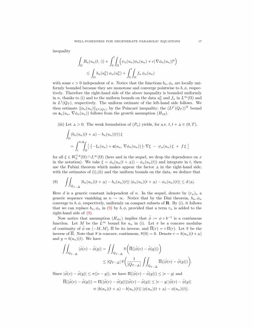
WELL-POSEDNESS FOR DEGENERATE PARABOLIC EQUATIONS 17
inequality ∫Ω
Bn(un(t, ·)) +∫ t
0
∫Ω
(ψn(un)φn(un) + c|∇φn(un)|p
)≤
∫Ω
bn(un0 )φn(un
0 ) +∫ t
0
∫Ω
fn φn(un)
with some c > 0 independent of n. Notice that the functions bn, φn are locally uni-formly bounded because they are monotone and converge pointwise to b, φ, respec-tively. Therefore the right-hand side of the above inequality is bounded uniformlyin n, thanks to (i) and to the uniform bounds on the data un
0 and fn in L∞(Ω) andin L1(QT ), respectively. The uniform estimate of the left-hand side follows. Wethen estimate ‖φn(un)‖Lp(QT ) by the Poincare inequality; the (Lp′(QT ))N boundon an(un, ∇φn(un)) follows from the growth assumption (H10).
(iii) Let ∆ > 0. The weak formulation of (Pn) yields, for a.e. t, t+ ∆ ∈ (0, T ),∫Ω
(bn(un)(t+ ∆)− bn(un)(t)) ξ
=∫ t+∆
t
∫Ω
[ (−fn(un) + a(un, ∇φn(un))
)·∇ξ − ψn(un) ξ + f ξ
]for all ξ ∈W 1,p
0 (Ω)∩L∞(Ω) (here and in the sequel, we drop the dependence on xin the notation). We take ξ = φn(un(t + ∆)) − φn(un(t)) and integrate in t, thenuse the Fubini theorem which makes appear the factor ∆ in the right-hand side;with the estimates of (i),(ii) and the uniform bounds on the data, we deduce that
(9)∫ ∫
QT−∆
|bn(un)(t+ ∆)− bn(un)(t)| |φn(un)(t+ ∆)− φn(un)(t)| ≤ d |∆|.
Here d is a generic constant independent of n. In the sequel, denote by (rn)n ageneric sequence vanishing as n → ∞. Notice that by the Dini theorem, bn, φn
converge to b, φ, respectively, uniformly on compact subsets of R. By (i), it followsthat we can replace bn, φn in (9) by b, φ, provided that a term rn is added to theright-hand side of (9).
Now notice that assumption (Hstr) implies that φ := φ b−1 is a continuousfunction. Let M be the L∞ bound for un in (i). Let π be a concave modulusof continuity of φ on [−M,M ], Π be its inverse, and Π(r) = rΠ(r). Let π be theinverse of Π. Note that π is concave, continuous, π(0) = 0. Denote v = b(un)(t+∆)and y = b(un)(t). We have∫ ∫
QT−∆
|φ(v)− φ(y)| =∫ ∫
QT−∆
π
(Π(|φ(v)− φ(y)|)
)≤ |QT−∆|π
(1
|QT−∆|
∫ ∫QT−∆
Π(|φ(v)− φ(y)|)).
Since |φ(v)− φ(y)| ≤ π(|v − y|), we have Π(|φ(v)− φ(y)|) ≤ |v − y| and
Π(|φ(v)− φ(y)|) = Π(|φ(v)− φ(y)|)|φ(v)− φ(y)| ≤ |v − y| |φ(v)− φ(y)|≡ |b(un)(t+ ∆)− b(un)(t)| |φ(un)(t+ ∆)− φ(un)(t)|.

18 B. ANDREIANOV, M. BENDAHMANE, K. H. KARLSEN, AND S. OUARO
Therefore the estimate (9) (with bn, φn and d∆ replaced by b, φ and d∆ + rn,respectively) implies∫ ∫
QT−∆
|φ(un)(t+∆)−φ(un)(t)|
≤ |QT−∆|π(
1|QT−∆|
∫ ∫QT−∆
|un(t+∆)− un(t)| |φ(un)(t+∆)− φ(un)(t)|)
= |QT−∆|π(
1|QT−∆|
∆
)≤ d π( d∆ + rn ),
and finally, replacing φ with φn we get
(10)∫ ∫
QT−∆
|φn(un(t+∆, x))−φn(un(t, x))| ≤ d π( d∆ + rn ) + rn.
Now using the fact that rn → 0 as n → ∞ and the fact that for all fixed n ∈ N,the left-hand side of (10) tends to zero as ∆ → 0, we deduce the claim of (iii).
6. Proof of the general continuous dependence property
In this section, we prove Theorem 2.2. First notice that the uniform estimatesof Lemma 5.1 and Lemma 3.2 apply. It follows that there exists a (not relabelled)subsequence (un)n such that• wn := φn(un) converges strongly in L1(QT ) and a.e. on QT to some function w;• wn converges weakly in Lp(0, T ;W 1,p
0 (Ω));• χn := a(un, ∇wn) converges weakly in Lp′(QT ) to some limit χ;• un converges to µ : QT × (0, 1) −→ R in the sense of the nonlinear weak-?convergence (3).
Denote u(·) =∫ 1
0µ(·, α) dα. Thanks to the uniform L∞ bound on un and to
the uniform convergence of φn to φ on compact subsets of R, we can identify thelimit of wn(·) with
∫ 1
0φ(µ(α, ·)) dα; moreover, φ(µ(α, ·)) is independent of α ∈ (0, 1),
because the convergence of φ(un) to w is actually strong. Thus w, φ(u) and φ(µ(α))coincide. We also identify the limit of ∇wn with ∇w, because the two functionscoincide as elements of D′.
The following lemma permits to deduce strong convergence of un to u on the set[u /∈ E] (recall that E is assumed to be closed).
Lemma 6.1. Let φn(·) be a sequence of continuous non-decreasing functions con-verging pointwise to a continuous function φ(·). Assume φ(·) is strictly increasingon R\E. Let I be an open interval contained in R\E, and φn(un) → φ(u) a.e. onQ. Then un → u a.e. on [u ∈ I].
Proof. Let I = (a, b) and choose I ′ = (a′, b′) with a < a′ < b′ < b. Introduce δ > 0by
δ := minφ(a′)− φ(a), φ(b)− φ(b′).Notice that by the Dini theorem, the convergence of φn(·) to φ(·) is uniform
on all compact subset of R. Thus for all ε > 0, there exists N ∈ N such that‖φn − φ‖C([a,b]) < ε/2. With ε = δ, it follows that for all n sufficiently large,φn(b) − φ(b′) = φn(b) − φ(b) + φ(b) − φ(b′) > −δ/2 + δ = δ/2, and similarly,φ(a′)− φn(a) > δ/2. By the monotonicity of φn(·), φ(·),
maxu∈I′, z /∈I
|φn(z)− φ(u)| = maxφn(b)− φ(b′), φ(a′)− φn(a) > δ/2.

WELL-POSEDNESS FOR DEGENERATE PARABOLIC EQUATIONS 19
Hence if u(t, x) ∈ I ′ and if |φn(un(t, x)) − φ(u(t, x))| < δ/2, we have un(t, x) ∈ I.Since for all ε > 0 there exists N ∈ N such that |φn(un(t, x)) − φ(u(t, x))| ≤ ε/2,we have in particular that for a.e. (t, x) ∈ [u ∈ I ′], one has un ∈ I for all n largeenough.
Thus for all ε < δ, for a.e. point of [u ∈ I ′] there exists N ∈ N such that at thispoint one has
|φ(un)− φ(u)| ≤ |φ(un)− φn(un)|+ |φn(un)− φ(u)|≤ ‖φn − φ‖C([a,b]) + ε/2 ≤ ε.
Therefore φ(un) converges to φ(u) a.e. on [u ∈ I ′]. Since φ(·) is continuouslyinvertible on I, one also has un → u a.e. on [u ∈ I ′]. Since I is open and I ′ b I isarbitrary, the claim of the lemma follows.
Now we start to identify χ with a(u, ∇w). First, according to Remark 1.2,a(u, ∇w) = 0 a.e. on the set [u ∈ E] = [w ∈ G]. Using Lemma 3.2, we now deducethat also χ = 0 on this set.
Lemma 6.2. Let χ be the weak Lp′(QT ) limit of the sequence
χn = an(un, ∇φn(un)),
and let wn = φn(un) converge to w = φ(u) a.e.. Then χ = 0 a.e. on [u ∈ E].Moreover, χn converges strongly to zero in L1([u ∈ E]).
Proof. Since 1l[u∈E] ∈ L∞(QT ) ⊂ Lp(QT ), by the definition of the weak conver-gence, the function χ1l[u∈E] ≡ χ1l[w∈G] is the weak (Lp′(QT ))N limit of χn1l[w∈G].For all ε > 0, choose an open set Gε ⊃ G of measure less than ε. Because wn → wa.e. and Gε is an open neighbourhood of G, we have
[u ∈ E] = [w ∈ G] = R ∪(∪N∈N[w ∈ G, wn ∈ Gε ∀n ≥ N ]
),
where meas (R) = 0. Since([w ∈ G, wn ∈ Gε ∀n ≥ N ]
)N∈N
is an increasing collection of sets, the corresponding sequence of measures convergesto meas ([w ∈ G]) as N →∞, by the continuity of the Lebesgue measure. Because
meas ([w ∈ G]) ≥ meas ([w ∈ G, wN ∈ Gε]) ≥ meas ([w ∈ G, wn ∈ Gε ∀n ≥ N ]),
we conclude that meas ([w ∈ G, wn /∈ Gε]) tends to zero as n → ∞. Now by theHolder inequality,
‖χn1l[w∈G]‖L1(Q) =∫ ∫
[w∈G]
|an(un, ∇wn)|
≤∫ ∫
[wn∈Gε]
|an(un, ∇wn)|
+(∫ ∫
QT
|an(un, ∇wn)|p′) 1
p′
×(
meas ([w ∈ G, wn /∈ Gε])) 1
p
.
For all fixed ε > 0, the last term tends to zero as n→∞, thanks to the boundednessof the sequence an(un, ∇wn) in Lp′(QT ). The first term in the right-hand side
20 B. ANDREIANOV, M. BENDAHMANE, K. H. KARLSEN, AND S. OUARO
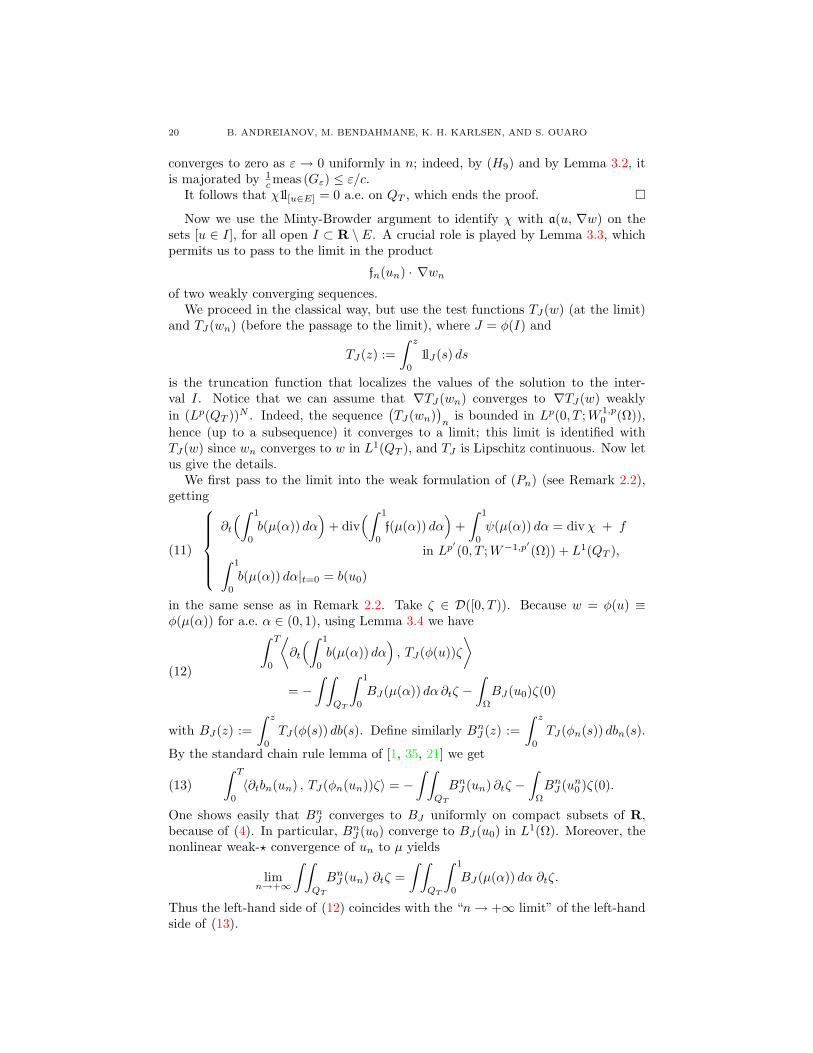
converges to zero as ε → 0 uniformly in n; indeed, by (H9) and by Lemma 3.2, itis majorated by 1
cmeas (Gε) ≤ ε/c.It follows that χ1l[u∈E] = 0 a.e. on QT , which ends the proof.
Now we use the Minty-Browder argument to identify χ with a(u, ∇w) on thesets [u ∈ I], for all open I ⊂ R \ E. A crucial role is played by Lemma 3.3, whichpermits us to pass to the limit in the product
fn(un) · ∇wn
of two weakly converging sequences.We proceed in the classical way, but use the test functions TJ(w) (at the limit)
and TJ(wn) (before the passage to the limit), where J = φ(I) and
TJ(z) :=∫ z
0
1lJ(s) ds
is the truncation function that localizes the values of the solution to the inter-val I. Notice that we can assume that ∇TJ(wn) converges to ∇TJ(w) weaklyin (Lp(QT ))N . Indeed, the sequence
(TJ(wn)
)n
is bounded in Lp(0, T ;W 1,p0 (Ω)),
hence (up to a subsequence) it converges to a limit; this limit is identified withTJ(w) since wn converges to w in L1(QT ), and TJ is Lipschitz continuous. Now letus give the details.
We first pass to the limit into the weak formulation of (Pn) (see Remark 2.2),getting
(11)
∂t
(∫ 1
0
b(µ(α)) dα)
+ div(∫ 1
0
f(µ(α)) dα)
+∫ 1
0
ψ(µ(α)) dα = divχ + f
in Lp′(0, T ;W−1,p′(Ω)) + L1(QT ),∫ 1
0
b(µ(α)) dα|t=0 = b(u0)
in the same sense as in Remark 2.2. Take ζ ∈ D([0, T )). Because w = φ(u) ≡φ(µ(α)) for a.e. α ∈ (0, 1), using Lemma 3.4 we have∫ T
0
⟨∂t
(∫ 1
0
b(µ(α)) dα), TJ(φ(u))ζ
⟩= −
∫ ∫QT
∫ 1
0
BJ(µ(α)) dα ∂tζ −∫
Ω
BJ(u0)ζ(0)(12)
with BJ(z) :=∫ z
0
TJ(φ(s)) db(s). Define similarly BnJ (z) :=
∫ z
0
TJ(φn(s)) dbn(s).
By the standard chain rule lemma of [1, 35, 21] we get
(13)∫ T
0
〈∂tbn(un) , TJ(φn(un))ζ〉 = −∫ ∫
QT
BnJ (un) ∂tζ −
∫Ω
BnJ (un
0 )ζ(0).
One shows easily that BnJ converges to BJ uniformly on compact subsets of R,
because of (4). In particular, BnJ (u0) converge to BJ(u0) in L1(Ω). Moreover, the
nonlinear weak-? convergence of un to µ yields
limn→+∞
∫ ∫QT
BnJ (un) ∂tζ =
∫ ∫QT
∫ 1
0
BJ(µ(α)) dα ∂tζ.
Thus the left-hand side of (12) coincides with the “n→ +∞ limit” of the left-handside of (13).
WELL-POSEDNESS FOR DEGENERATE PARABOLIC EQUATIONS 21
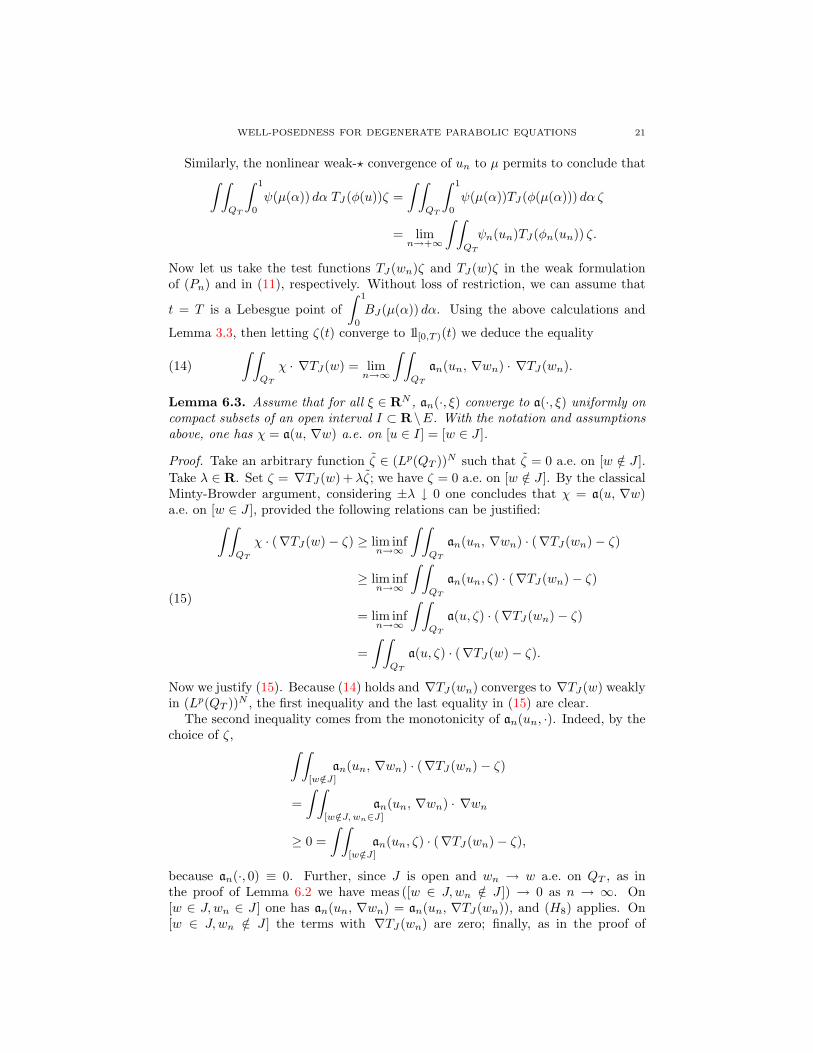
Similarly, the nonlinear weak-? convergence of un to µ permits to conclude that∫ ∫QT
∫ 1
0
ψ(µ(α)) dα TJ(φ(u))ζ =∫ ∫
QT
∫ 1
0
ψ(µ(α))TJ(φ(µ(α))) dα ζ
= limn→+∞
∫ ∫QT
ψn(un)TJ(φn(un)) ζ.
Now let us take the test functions TJ(wn)ζ and TJ(w)ζ in the weak formulationof (Pn) and in (11), respectively. Without loss of restriction, we can assume that
t = T is a Lebesgue point of∫ 1
0
BJ(µ(α)) dα. Using the above calculations and
Lemma 3.3, then letting ζ(t) converge to 1l[0,T )(t) we deduce the equality
(14)∫ ∫
QT
χ · ∇TJ(w) = limn→∞
∫ ∫QT
an(un, ∇wn) · ∇TJ(wn).
Lemma 6.3. Assume that for all ξ ∈ RN , an(·, ξ) converge to a(·, ξ) uniformly oncompact subsets of an open interval I ⊂ R \E. With the notation and assumptionsabove, one has χ = a(u, ∇w) a.e. on [u ∈ I] = [w ∈ J ].
Proof. Take an arbitrary function ζ ∈ (Lp(QT ))N such that ζ = 0 a.e. on [w /∈ J ].Take λ ∈ R. Set ζ = ∇TJ(w) +λζ; we have ζ = 0 a.e. on [w /∈ J ]. By the classicalMinty-Browder argument, considering ±λ ↓ 0 one concludes that χ = a(u, ∇w)a.e. on [w ∈ J ], provided the following relations can be justified:∫ ∫
QT
χ · (∇TJ(w)− ζ) ≥ lim infn→∞
∫ ∫QT
an(un, ∇wn) · (∇TJ(wn)− ζ)
≥ lim infn→∞
∫ ∫QT
an(un, ζ) · (∇TJ(wn)− ζ)
= lim infn→∞
∫ ∫QT
a(u, ζ) · (∇TJ(wn)− ζ)
=∫ ∫
QT
a(u, ζ) · (∇TJ(w)− ζ).
(15)
Now we justify (15). Because (14) holds and ∇TJ(wn) converges to ∇TJ(w) weaklyin (Lp(QT ))N , the first inequality and the last equality in (15) are clear.
The second inequality comes from the monotonicity of an(un, ·). Indeed, by thechoice of ζ, ∫ ∫
[w/∈J]
an(un, ∇wn) · (∇TJ(wn)− ζ)
=∫ ∫
[w/∈J, wn∈J]
an(un, ∇wn) · ∇wn
≥ 0 =∫ ∫
[w/∈J]
an(un, ζ) · (∇TJ(wn)− ζ),
because an(·, 0) ≡ 0. Further, since J is open and wn → w a.e. on QT , as inthe proof of Lemma 6.2 we have meas ([w ∈ J,wn /∈ J ]) → 0 as n → ∞. On[w ∈ J,wn ∈ J ] one has an(un, ∇wn) = an(un, ∇TJ(wn)), and (H8) applies. On[w ∈ J,wn /∈ J ] the terms with ∇TJ(wn) are zero; finally, as in the proof of
22 B. ANDREIANOV, M. BENDAHMANE, K. H. KARLSEN, AND S. OUARO
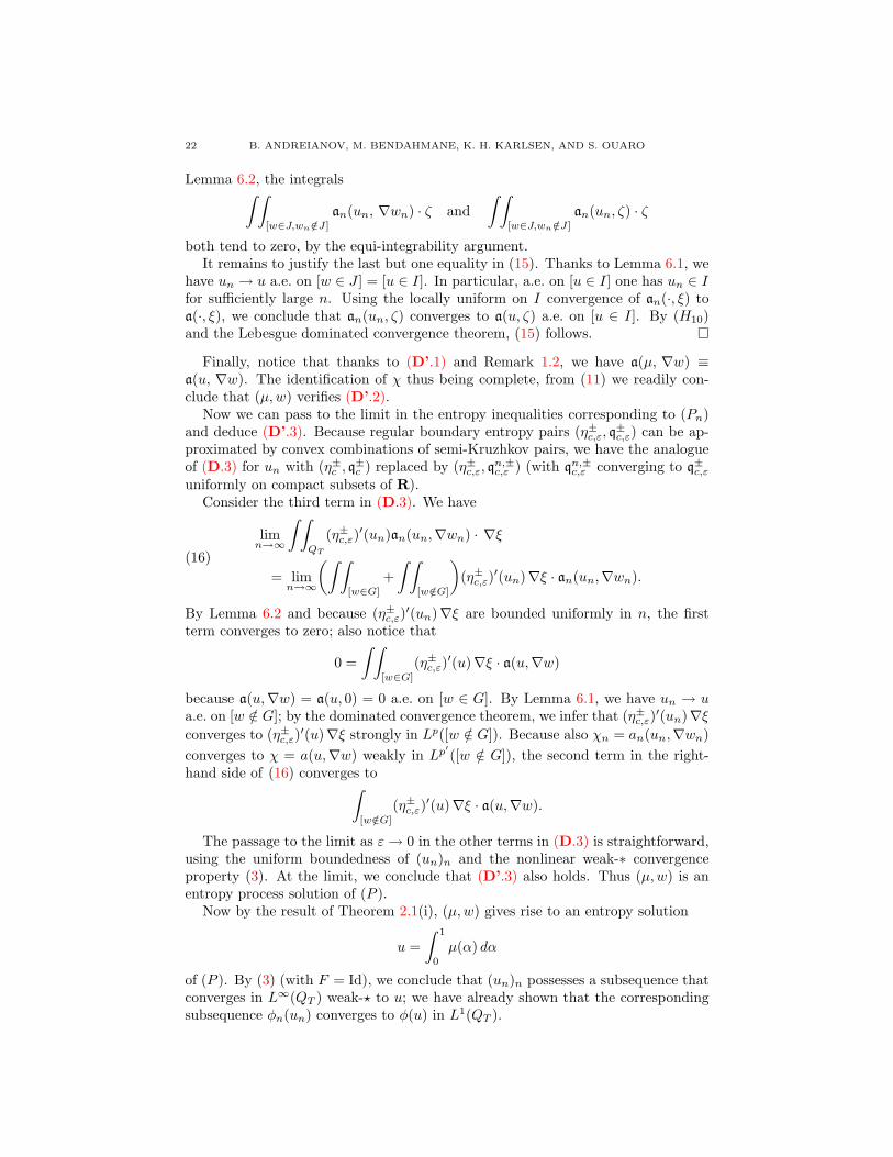
Lemma 6.2, the integrals∫ ∫[w∈J,wn /∈J]
an(un, ∇wn) · ζ and∫ ∫
[w∈J,wn /∈J]
an(un, ζ) · ζ
both tend to zero, by the equi-integrability argument.It remains to justify the last but one equality in (15). Thanks to Lemma 6.1, we
have un → u a.e. on [w ∈ J ] = [u ∈ I]. In particular, a.e. on [u ∈ I] one has un ∈ Ifor sufficiently large n. Using the locally uniform on I convergence of an(·, ξ) toa(·, ξ), we conclude that an(un, ζ) converges to a(u, ζ) a.e. on [u ∈ I]. By (H10)and the Lebesgue dominated convergence theorem, (15) follows.
Finally, notice that thanks to (D’.1) and Remark 1.2, we have a(µ, ∇w) ≡a(u, ∇w). The identification of χ thus being complete, from (11) we readily con-clude that (µ,w) verifies (D’.2).
Now we can pass to the limit in the entropy inequalities corresponding to (Pn)and deduce (D’.3). Because regular boundary entropy pairs (η±c,ε, q
±c,ε) can be ap-
proximated by convex combinations of semi-Kruzhkov pairs, we have the analogueof (D.3) for un with (η±c , q
±c ) replaced by (η±c,ε, q
n,±c,ε ) (with qn,±
c,ε converging to q±c,ε
uniformly on compact subsets of R).Consider the third term in (D.3). We have
limn→∞
∫ ∫QT
(η±c,ε)′(un)an(un,∇wn) · ∇ξ
= limn→∞
(∫ ∫[w∈G]
+∫ ∫
[w/∈G]
)(η±c,ε)
′(un)∇ξ · an(un,∇wn).(16)
By Lemma 6.2 and because (η±c,ε)′(un)∇ξ are bounded uniformly in n, the first
term converges to zero; also notice that
0 =∫ ∫
[w∈G]
(η±c,ε)′(u)∇ξ · a(u,∇w)
because a(u,∇w) = a(u, 0) = 0 a.e. on [w ∈ G]. By Lemma 6.1, we have un → ua.e. on [w /∈ G]; by the dominated convergence theorem, we infer that (η±c,ε)
′(un)∇ξconverges to (η±c,ε)
′(u)∇ξ strongly in Lp([w /∈ G]). Because also χn = an(un,∇wn)converges to χ = a(u,∇w) weakly in Lp′([w /∈ G]), the second term in the right-hand side of (16) converges to∫
[w/∈G]
(η±c,ε)′(u)∇ξ · a(u,∇w).
The passage to the limit as ε→ 0 in the other terms in (D.3) is straightforward,using the uniform boundedness of (un)n and the nonlinear weak-∗ convergenceproperty (3). At the limit, we conclude that (D’.3) also holds. Thus (µ,w) is anentropy process solution of (P ).
Now by the result of Theorem 2.1(i), (µ,w) gives rise to an entropy solution
u =∫ 1
0
µ(α) dα
of (P ). By (3) (with F = Id), we conclude that (un)n possesses a subsequence thatconverges in L∞(QT ) weak-? to u; we have already shown that the correspondingsubsequence φn(un) converges to φ(u) in L1(QT ).
WELL-POSEDNESS FOR DEGENERATE PARABOLIC EQUATIONS 23
Moreover, b(µ(α)) and ψ(µ(α)) are in fact independent of α. By Theorem 2.1(iii),we also have the uniqueness of b(u) and ψ(u) such that u is an entropy solutionof (P ). By the well-known result of the nonlinear weak-? convergence (see e.g.,Hungerbuhler [26]), it follows that the whole sequences (bn(un))n and (ψn(un))n
converge to b(u) and ψ(u), respectively, in measure on QT and in L1(QT ).This ends the proof of Theorem 2.2.
Remark 6.1. In the case assumption (H5) is dropped, in order to deduce that u isan entropy process solution, along with the assumption (Hstr) one needs a growthrestriction on f of the following kind: there exists a function M ∈ C(R+;R+) anda function L with lim
z→+∞L(z)/z = 0 such that
|f(b(r), φ(r), ψ(r))| ≤M(|b(r)|) L(|φ(r)|p+
∫ r
0
φ(s) db(s) + ψ(r)φ(r))
for all r ∈ R, and the same assumption with |f(b(r), φ(r), ψ(r))| replaced with |b(r)|and with |ψ(r)|. Indeed, these inequalities make it possible to use the nonlinearweak-? convergence framework of Ball [8] and Hungerbuhler [26] without the uniformL∞ bound on (un)n.
7. Proof of Theorem 2.3
In this section, we prove Theorem 2.3. The uniqueness claim was shown inTheorem 2.1; also notice that the continuous dependence result under the structureassumption (Hstr) was shown in Theorem 2.2. Let us first prove the existence claim.
(i) First, consider the case where assumption (Hstr) is fulfilled. Consider anapproximation of (P ) by regular problems (Pn) with data (bn, ψ, φn, a, f;u0, f) suchthat the assumptions of Theorem 2.2 are fulfilled, and bn, [bn]−1, fn, φn, [φn]−1 areLipschitz continuous on R. Using classical methods (cf. Alt and Luckhaus [1],Lions [30]), one shows that there exists a weak solution un ∈ Lp(0, T ;W 1,p
0 (Ω)) tothe problem (Pn) in the sense
∂tbn(un) + div fn(un) + ψ(un) = div a(un, ∇φn(un)) + f
in Lp′(0, T ;W−1,p′(Ω)) + L1(QT ), with initial data
bn(un)|t=0 = bn(u0).
In addition, un verifies the entropy formulation (D.3), obtained along the lines ofCarrillo [20]. By Theorem 2.2, we conclude that there exists an entropy solution of(P ).
To prove existence without the structure condition (Hstr), we use the particularmulti-step approximation approach of Ammar and Wittbold [4] (see also Ammarand Redwane [3]). We replace b by bk := b+ 1
k Id and ψ, by ψm,n := ψ+ 1n Id++ 1
m Id−.The result of (i) for the corresponding problem (P k
m,n) is already proved.There exists a function uk
m,n, constructed by means of the nonlinear semigrouptheory (see e.g., [12]), such that bk(uk
m,n) is the unique integral solution to theabstract evolution problem associated with (P k
m,n) (here and below, we refer toAmmar and Wittbold [4], Ammar and Redwane [3] for details). One then showsthat uk
m,n coincides with the unique entropy solution of (P km,n), the existence of this
entropy solution being already shown. Further, the whole set (ukm,n)k,m,n verifies
the uniform a priori estimates of Lemmas 5.1, 3.2.

24 B. ANDREIANOV, M. BENDAHMANE, K. H. KARLSEN, AND S. OUARO
We then pass to the limit in ukm,n in the following order: first k → +∞, then
n→ +∞, m→ +∞.While letting k → +∞, we use the fact that ψ−1
m,n is Lipschitz continuous. Thefundamental estimates for the semigroup solutions permit to show that ψm,n(um,n)are uniformly continuous on (0, T ) with values in L1(Ω); thus we get the strongprecompactness of (uk
m,n)k in L1(QT ). Thus, up to a subsequence, ukm,n converge
to um,n which is an entropy solution of problem (Pm,n) corresponding to the data(b, ψm,n, φ, a, f;u0, f).
Finally, we use the inequalities um+1,n ≤ um,n ≤ um,n+1 which follow readilyform the comparison principle of Theorem 2.1(ii). The monotonicity argumentyields the strong convergence of um,n. Now the whole scheme of the proof ofTheorem 2.2 applies with considerable simplifications, because no nonlinear weak-?convergence arguments are not needed. Passing to the limit in um,n, we concludethat the limit u is an entropy solution of the original problem (P ). This ends theexistence proof.
(ii) Existence for the limit data (u0, f) is now shown and we can apply Theo-rem 2.1(ii). Then we deduce the L1(QT ) convergence of b(un), ψ(un) to b(u), ψ(u),respectively. The convergence of φ(un) to φ(u) in L1(QT ) follows, by hypothesis(H ′
str) and because our assumptions imply the uniform L∞(QT ) bound on un.The remaining claim of the strong (Lp(QT ))N convergence of ∇φ(un) is a rather
standard part of the Minty-Browder trick. The argument is based upon the proofof Theorem 2.2. Because we already have the strong compactness of (φ(un))n, wecan bypass the hypothesis (Hstr) and deduce that the L∞ weak-? limit u of un isan entropy solution of (P ) with the data (u0, f). In particular, the (Lp′(QT ))N
weak limit χ of a(un, ∇φ(un)) is equal to a(u, ∇φ(u)). Now notice that by The-orem 2.1(iii), under the structure condition (H ′
str) we also have the uniqueness ofφ(u) such that u is an entropy solution of (P ); moreover, by Remark 1.2, we alsohave the uniqueness of a(u, ∇φ(u)) such that u is an entropy solution of (P ). Thusχ coincides with a(u, ∇φ(u)), so that (14) now reads as
(17)∫ ∫
QT
a(u,∇φ(u)) · ∇φ(u) = limn→∞
∫ ∫QT
an(un,∇wn) · ∇φ(un).
It follows by the weak convergences of ∇φ(un) and of a(un, ∇φ(un)) that
(18) limn→∞
∫ ∫QT
(a(u,∇φ(u))− a(un,∇φ(un))
)·(∇φ(u)− ∇φ(un)
)= 0.
Notice that a.e. on the set [u ∈ E], ∇φ(un) converges to 0 = ∇φ(u), by Lemma 6.2and by the coercivity assumption (H9). On the set [u /∈ E], we can use Lemma 6.1to replace a(u,∇φ(u)) with a(un,∇φ(u)) in the above formula (18). Using theuniform monotonicity assumption (H ′
8), we can now conclude that the convergenceof ∇φ(un) to ∇φ(u) holds a.e. on QT .
Separating again the sets [u ∈ E] and [u /∈ E], we deduce that the sequenceof nonnegative functions a(un,∇φ(un)) · ∇φ(un) converges to a(u,∇φ(u)) · ∇φ(u)a.e. on QT . Together with (17), this implies that a(un,∇φ(un)) · ∇φ(un) also con-verge to a(u,∇φ(u)) · ∇φ(u) in L1(QT ); in particular, they are equi-integrable onQT . The coercivity assumption (H9) now implies the equi-integrability on QT ofthe functions |∇φ(un)|p. Combining this argument with the a.e. convergence of∇φ(un), we deduce our claim from the Vitali theorem. The (Lp′(QT ))N conver-gence of a(un, ∇φ(un)) to a(u, ∇φ(u)) follows in the same way.
WELL-POSEDNESS FOR DEGENERATE PARABOLIC EQUATIONS 25
8. Well-posedness for the doubly nonlinear elliptic problem
We first notice that the well-posedness result for the degenerate elliptic problem
(S)ψ(u) + div f(ψ(u), φ(u))− div a(u, ∇φ(u)) = s in Ω,u = 0 on ∂Ω
(H ′5) s ∈ L∞(Ω) and ψ(R) = R
follows from Theorem 2.3, upon setting b ≡ 0, f(t, ·) ≡ s(·) and arbitrarily prescrib-ing u0. The definition of an entropy solution of (S) can also be formally obtainedfrom Definition 2.2.
Let us notice that the analogue of the general continuous dependence propertyof Theorem 2.2 holds without any additional structure condition:
Theorem 8.1. Let (ψn, φn, an, fn; s), n ∈ N, be a sequence converging to (ψ, φ, a, f; s)in the following sense:
· ψn, φn converge pointwise to ψ, φ respectively;· fn, an converge to f, a, respectively, uniformly on compacts;· sn converges to s in L1(Ω).
Assume that (ψ, φ, a, f; s) and (ψn, φn, an, fn; sn) (for each n) satisfy the hypotheses(H1), (H6)-(H11), and (H ′
5), and, moreover, that the functions C in (H9), (H10),and (H11) as well as the L∞(Ω) bound in (H ′
5) are independent of n. We denoteby (Sn) the analogue of problem (S) corresponding to the data and coefficients(ψn, φn, an, fn; sn).
Assume that φ satisfies the technical hypotheses (H2),(H3).Let un be an entropy solution of problem (Sn). Then the functions un converge to
an entropy solution u of (S) in L∞(Ω) weakly-*, up to a subsequence. Furthermore,the functions φn(un) converge to φ(u) in Lp(Ω) up to a subsequence, and the wholesequence ψn(un) converges to ψ(u) in L1(Ω).
The proof of Theorem 8.1 is contained in the one of Theorem 2.2, because the Lp(Ω)bound on ∇wn is sufficient for the strong precompactness of wn.
26 B. ANDREIANOV, M. BENDAHMANE, K. H. KARLSEN, AND S. OUARO
References
[1] H. W. Alt and S. Luckhaus. Quasilinear elliptic-parabolic differential equations. Math. Z.,183(3):311–341, 1983.
[2] K. Ammar, P. Wittbold and J. Carrillo. Scalar conservation laws with general boundary
condition and continuous flux function. J. Diff. Eq.. 228(1):111–139, 2006.[3] K. Ammar and H.Redwane. Degenerate stationary problems with homogeneous boundary
conditions. Electronic J. Diff. Eq. 2008(30):1–18, 2008.
[4] K. Ammar and P. Wittbold. Existence of renormalized solutions of degenerate elliptic-parabolic problems. Proc. Roy. Soc. Edinburgh Sect. A 133(3):477–496, 2003.
[5] B. Andreianov. Some problems of the theory of nonlinear degenerate parabolic systems andconservation laws. Ph.D. thesis, Univ. de Franche-Comte, 2000.
[6] B. Andreianov, M. Bendahmane and K. H. Karlsen. Finite volume schemes for doubly non-
linear degenerate parabolic equations, in preparation[7] B. Andreianov and N. Igbida. Uniqueness for inhomogeneous Dirichlet problem for elliptic-
parabolic equations. Proc. Royal Soc. Edinburgh A, 137(6):1119–1133, 2007.[8] J.M. Ball. A version of the fundamental theorem for Young measures. in PDEs and Continuum
Models of Phase Transitions (Nice, 1988), Lecture Notes in Phys. 344, Springer, Berlin, 1989,
207215.[9] C. Bardos, A. Y. LeRoux and J.-C. Nedelec. First order quasilinear equations with boundary
conditions. Comm. Partial Differential Equations, 4(9):1017–1034, 1979.
[10] M. Bendahmane and K. H. Karlsen. Renormalized entropy solutions for quasilinearanisotropic degenerate parabolic equations. SIAM J. Math. Anal., 36(2):405–422, 2004.
[11] M. Bendahmane and K. H. Karlsen. Uniqueness of entropy solutions for doubly nonlinear
anisotropic degenerate parabolic equations. Contemporary Mathematics, 371, Amer. Math.Soc., pp.1–27, 2005.
[12] Ph. Benilan, M.G. Crandall and A. Pazy. Nonlinear evolution equations in banach spaces.
preprint book.[13] P. Benilan and H. Toure. Sur l’equation generale ut = a(·, u, φ(·, u)x)x + v dans L1. II. Le
probleme d’evolution. Ann. Inst. H. Poincare Anal. Non Lineaire, 12(6):727–761, 1995.
[14] P. Benilan and P. Wittbold. On mild and weak solutions of elliptic-parabolic problems. Adv.Differential Equations, 1(6):1053–1073, 1996.
[15] A. Benkirane and J. Bennouna. Existence of solutions for nonlinear elliptic degenerate equa-
tions. Nonlinear Anal., 54(1):9–37, 2003.[16] A. Benkirane and A. Elmahi. An existence theorem for a strongly nonlinear elliptic problem
in Orlicz spaces. Nonlinear Anal. TMA, 36(1):11-24, 1999.[17] D. Blanchard and A. Porretta. Stefan problems with nonlinear diffusion and convection. J.
Diff. Eq., 210(2):383–428, 2005.[18] D. Blanchard and H. Redwane. Solutions renormalisees d’equations paraboliques a deux non
linearites. C. R. Acad. Sci. Paris Ser. I Math. 319(8):831–835, 1994.[19] D. Blanchard and H. Redwane. Renormalized solutions for a class of nonlinear evolution
problems. J. Math. Pures Appl. 77(2):117–151, 1998.[20] J. Carrillo. Entropy solutions for nonlinear degenerate problems. Arch. Rational Mech. Anal.,
147(4):269–361, 1999.
[21] J. Carrillo and P. Wittbold. Uniqueness of renormalized solutions of degenerate elliptic-parabolic problems. J. Differential Equations, 156(1):93–121, 1999.
[22] G.Q Chen and H. Frid. Divergence-measure fields and hyperbolic conservation laws. Arch.Rational Mech. Anal., 147(1999), pp. 89-118.
[23] R. Eymard, T. Gallouet and R. Herbin. Finite Volume Methods. Handbook of Numerical
Analysis, Vol. VII, P. Ciarlet, J.-L. Lions, eds., North-Holland, 2000.[24] R. Eymard, T. Gallouet, R. Herbin and A. Michel. Convergence of a finite volume scheme
for nonlinear degenerate parabolic equations. Numer. Math., 92(1):41–82, 2002.
[25] T. Gallouet and F. Hubert. On the convergence of the parabolic approximation of a conser-vation law in several space dimensions. no. 1, 141. Chinese Ann. Math. Ser. B, 20(1):7-10,
1999.
[26] N. Hungerbuhler. A refinement of Balls theorem on Young measures. New York J. Math.3:4853, 1997.
WELL-POSEDNESS FOR DEGENERATE PARABOLIC EQUATIONS 27
[27] J. Kacur. On a solution of degenerate elliptic-parabolic problems in Orlicz-Sobolev
spaces.I,II., Mat.Z. 203:153-171 and 569-579, 1990.[28] S. N. Kruzkov. First order quasi-linear equations in several independent variables. Math.
USSR Sbornik, 10(2):217–243, 1970.
[29] J. Leray and J.-L. Lions. Quelques resultats de Visik sur les problemes elliptiques non lineaires
par les methodes de Minty-Browder. Bull.Soc.Math. de France, 93:97-107, 1965.[30] J.-L. Lions. Quelques methodes de resolution des problemes aux limites non lineaires. Dunod,
1969.[31] J. Malek, J. Necas, M. Rokyta and M. Ruzicka. Weak and measure-valued solutions to evo-
lutionary PDEs. Chapman & Hall, London, 1996.
[32] C. Mascia, A. Porretta and A. Terracina. Nonhomogeneous dirichlet problems for degenerate
parabolic-hyperbolic equations. Arch. Ration. Mech. Anal., 163(2):87–124, 2002.[33] A. Michel and J. Vovelle. Entropy formulation for parabolic degenerate equations with general
Dirichlet boundary conditions and application to the convergence of FV methods. SIAM J.Numer. Anal. 41(6):2262–2293, 2003.
[34] F. Otto. Initial-boundary value problem for a scalar conservation law. C. R. Acad. Sci. Paris
Ser. I Math., 322(8):729–734, 1996.[35] F. Otto. L1-contraction and uniqueness for quasilinear elliptic-parabolic equations. J. Differ-
ential Equations, 131(1):20–38, 1996.[36] S. Ouaro. Entropy solutions of nonlinear elliptic-parabolic-hyperbolic degenerate problems in
one dimension. Int. J. Evol. Equ. 3(1):1–18, 2007.[37] S. Ouaro and H. Toure. Sur un probleme de type elliptique parabolique non lineaire. C. R.
Math. Acad. Sci. Paris 334(1):27–30, 2002.[38] S. Ouaro and H. Toure. On some nonlinear elliptic-parabolic equations of second order. Int.
J. Pure Appl. Math. 25(2)2:255–265, 2005.[39] S. Ouaro and H. Toure. Uniqueness of entropy solutions to nonlinear elliptic-parabolic prob-
lems. Electron. J. Diff. Eq., (82):1-15, 2007.
(Boris Andreianov)
Laboratoire de MathematiquesUniversite de Franche-Comte
16 route de Gray
25 030 Besanc, on Cedex, FranceE-mail address: [email protected]
(Mostafa Bendahmane)LAMFA, UMR-CNRS 6140
Universite de Picardie Jules Verne,
33 rue Saint Leu, 80038 Amiens, FranceE-mail address: mostafa [email protected]
(Kenneth H. Karlsen)Centre of Mathematics for Applications
University of Oslo
P.O. Box 1053, BlindernN–0316 Oslo, Norway
E-mail address: [email protected]
URL: http://folk.uio.no/kennethk
(Stanislas Ouaro)
Laboratoire d’Analyse Mathematique des Equations LAME
UFR Sciences Exactes et Appliquees, University of Ouagadougou
03 BP 7021 Ouaga 03Ouagadougou, Burkina-Faso
E-mail address: [email protected]