Observation Driven Models for Poisson Counts

Richard A. Davis, William T.M. Dunsmuir and Sarah B. Streett

December 24, 2001

AbstractThis paper is concerned with a general class of observation driven models for time

series of counts whose conditional distributions given past observations and explanatoryvariables follow a Poisson distribution. These models provide a flexible frameworkfor modeling a wide range of dependence structures. Conditions for stationarity andergodicity of these processes are established from which the large sample propertiesof the maximum likelihood estimators can be derived. Simulations are provided togive additional insight into the finite sample behavior of the estimates. Finally anapplication to a regression model for daily counts of accident and emergency roompresentations for asthma at several Sydney hospitals is described.

1 Introduction

In recent years there has been considerable development of models for non-Gaussian timeseries. In particular the special case of Poisson observations is of interest in a variety ofapplications including the modeling of the effects of environmental pollution on human healthand the impact of policy controls on road deaths. Davis et al. (1999) provides a review ofmodels for Poisson time series. There, the classification due to Cox (1981) of models intoobservation and parameter driven processes is described. In particular a new class of models,which we will refer to as generalized linear autoregressive moving average (GLARMA) modelsis introduced and its properties developed in part. The purpose of this paper is to developthese models more comprehensively.

In general terms, parameter driven models require considerable computational effort inorder to obtain parameter estimates - see Durbin and Koopman (2000) and Jung and Liesen-feld (2001) for recent contributions to this topic. In addition, because they are built on alatent process, forecasting also requires considerable computational effort. Parameter drivenmodels are, however, straightforward in their interpretation of the effects of covariates onthe observed count process, an appealing point.

Observation driven models are sometimes referred to as transition models in the longi-tudinal data analysis literature (e.g., see Diggle, Liang and Zeger, 1994). Zeger and Qaqish(1988) review various observation driven models for count time series. In particular they im-ply various desirable properties that such models should possess. First, the marginal meanof Yt should be approximated as

E(Yt) = E(µt) ≈ exp(xTt β)

1

so that the regression coefficients can be interpreted as the proportional change in themarginal expectation of Yt on the logarithm scale given a unit change in the regressorvariables. This seems useful from the point of view of interpretation. Additionally, forstationary processes, both positive and negative serial dependence should be possible. Someof the models that are discussed in Zeger and Qaqish (1988) do not satisfy this last propertyand will admit stationary solutions only for negative serial dependence, a case that is lesscommon in many applications than that of positive dependence.

To develop the class of models that are considered here, let

Ht = (Y(t−1),x(t))

be the past of the observed count process and the past and present of the regressor variables.Assume that the conditional distribution of Yt|Ht is Poisson with mean µt. A simple andappealing way to build serial dependence in the model is to require the log-mean process todepend linearly on previous observations. That is,

log(µt) = xTt β +

p∑i=1

γiYt−i. (1)

Note that the Yt−i enter without any form of mean correction or centering. Model (1) isapplied to data in Fahrmier and Tutz (1994). Zeger and Qaqish (1988) point out that (1)cannot be stationary unless, at least in the case p = 1 , γ1 ≤ 0 thereby excluding thepossibility of positive dependence. This point is also acknowledged by Fahrmier and Tutz.It might be thought that the difficulties with model (1) could be overcome by subtractingthe ‘fixed effects’ component of the mean from the Yt to arrive at

µt = exp(xTt β +

p∑i=1

γi(Yt−i − exp(xTt β)), (2)

but in fact this will not lead to a stationary process as can be seen by using a similar argumentto that given by Zeger and Qaqish (1988). In an unpublished report Shephard (1995) extends(2) by using the standardized deviations (Yt−i − exp(xTt β))/ exp(xTt β) and by including lagstructure that corresponds to rational functions similar to those for autoregressive movingaverage linear models. In a later unpublished paper Rydberg and Shephard (1998) considermodels with exponential family distributions conditional on Ht which are analogous but forwhich the standardization uses conditional standard deviations rather than variances. Daviset al. (1999) consider a general class of models that allows for normalization to occur withvarious powers of the conditional variance including those considered by Shephard (1995)and Rydberg and Shephard (1998). In line with terminology introduced by Shephard (1995)we will refer to this general class of models as GLARMA models.

Observation driven models are generally very easy to fit using conditional maximumlikelihood. Here conditioning refers to conditioning on some initial values and not on randomeffects. Also forecasting of future observations is straightforward. However, because of theway in which past observations feed into the mean term, the interpretation of the effect ofcovariates can be confused to varying extents depending on the form of the model.

2

In many practical problems, the primary objective is to develop models that relate co-variates, such as environmental or policy intervention variables, to the observed time seriesof counts, such as the daily number of asthma cases at a hospital. Often there are numerouscovariates that may need to be considered for inclusion in the model. In some instances,many comparable time series of counts need to be modeled as part of a larger study. Forexample, in studying the impact of alcohol or traffic regulation policy interventions on roaddeaths or youth suicides, all regions or states in a country may need to be considered sepa-rately since the timing and nature of these variables may have regional variations. In thesesettings there is a distinct advantage to have methods available that are easy to implementand rapid to compute for investigating the impact of covariates on time series of counts whichproperly control for serial dependence. At the present time, and for realistically long andnumerous time series arising in the areas we have described, the computationally intensivemethods required for fitting parameter driven models are not yet routinely available. Thispaper develops a class of observation driven models that are straightforward to implementand are rapid to fit. In addition, these models adjust for serial dependence in the inferencefor fixed effects and allow reasonable interpretations of the effects of these covariates on theresponse variable.

Our observation driven model is introduced in Section 2, where general properties aboutthe process are also given. In Section 3, we consider maximum likelihood estimates for thesemodels with supporting simulation results. Section 4 contains an application of fitting thesemodels to data consisting of the number of asthma presentations at a hospital in the Sydneymetropolitan area. Technical results related to the the properties of the process and theasymptotic normality of the maximum likelihood estimator are given in Section 5.

2 Observation Driven Models

2.1 The Basic Model

To introduce our model, assume that the observation Yt given the past history Ft−1 =σ(Ys, s ≤ t− 1) is Poisson with mean µt which will be denoted by

Yt|Ft−1 ∼ P (µt).

It is further assumed that the state process log(µt) follows a linear model in the explanatoryvariables with residuals that have a moving average structure. The noise driving the movingaverage will be a martingale difference sequence generated from the data and hence the nameobservation driven model. Formally, the state process is given by

Wt := log(µt) = xTt β +

q∑i=1

θiet−i,

whereet = (Yt − µt)/µλt , λ ≥ 0.

Since the conditional mean E(Yt|Y(t−1)) depends on the whole past, the process Yt isno longer Markov. However, the mean process log(µt) is qth order Markov. Unless xTt β isconstant, log(µt) is not a time-homogeneous process.

3

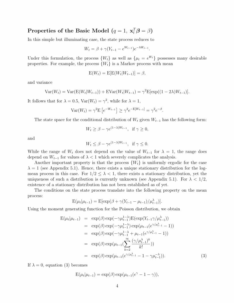
Properties of the Basic Model (q = 1, xTt β = β)

In this simple but illuminating case, the state process reduces to

Wt = β + γ(Yt−1 − eWt−1)e−λWt−1 .

Under this formulation, the process Wt as well as µt = eWt possesses many desirableproperties. For example, the process Wt is a Markov process with mean

E(Wt) = E[E(Wt|Wt−1)] = β,

and variance

Var(Wt) = Var(E(Wt|Wt−1)) + EVar(Wt|Wt−1) = γ2E[exp((1− 2λ)Wt−1)].

It follows that for λ = 0.5, Var(Wt) = γ2, while for λ = 1,

Var(Wt) = γ2E

[e−Wt−1

] ≥ γ2e−E[Wt−1] = γ2e−β.

The state space for the conditional distribution of Wt given Wt−1 has the following form:

Wt ≥ β − γe(1−λ)Wt−1 , if γ ≥ 0,

andWt ≤ β − γe(1−λ)Wt−1 , if γ ≤ 0.

While the range of Wt does not depend on the value of Wt−1 for λ = 1, the range doesdepend on Wt−1 for values of λ < 1 which severely complicates the analysis.

Another important property is that the process Wt is uniformly ergodic for the caseλ = 1 (see Appendix 5.1). Hence, there exists a unique stationary distribution for the log-mean process in this case. For 1/2 ≤ λ < 1, there exists a stationary distribution, yet theuniqueness of such a distribution is currently unknown (see Appendix 5.1). For λ < 1/2,existence of a stationary distribution has not been established as of yet.

The conditions on the state process translate into the following property on the meanprocess:

E(µt|µt−1) = E[exp(β + γ(Yt−1 − µt−1)/µλt−1)].

Using the moment generating function for the Poisson distribution, we obtain

E(µt|µt−1) = exp(β) exp(−γµ1−λt−1 )E(exp(Yt−1γ/µ

λt−1))

= exp(β) exp(−γµ1−λt−1 ) exp(µt−1(e

γ/µλt−1 − 1))

= exp(β) exp(−γµ1−λt−1 + µt−1(e

γ/µλt−1 − 1))

= exp(β) exp(µt−1(∞∑k=2

(γ/µλt−1)k

k!))

= exp(β) exp(µt−1(eγ/µλ

t−1 − 1− γµ−λt−1)). (3)

If λ = 0, equation (3) becomes

E(µt|µt−1) = exp(β) exp(µt−1(eγ − 1− γ)),

4

so that if γ ≥ 0 the conditional means will evolve in an unstable fashion. Thus, whenλ = 0, E(µt|µt−1) will grow without bound whenever µt becomes positive. In contrast, forλ = 1, equation (3) becomes

E(µt|µt−1) = exp(β − γ) exp(µt−1(eγ/µt−1 − 1)),

which is bounded as µt → ∞. For other values, 0 < λ < 1, the stability properties of theprocess are less clear.

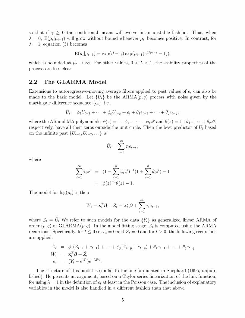
2.2 The GLARMA Model

Extensions to autoregressive-moving average filters applied to past values of et can also bemade to the basic model. Let Ut be the ARMA(p, q) process with noise given by themartingale difference sequence et, i.e.,

Ut = φ1Ut−1 + · · ·+ φpUt−p + et + θ1et−1 + · · ·+ θqet−q ,where the AR and MA polynomials, φ(z) = 1−φ1z−· · ·−φpzp and θ(z) = 1+θ1z+· · ·+θqzq,respectively, have all their zeros outside the unit circle. Then the best predictor of Ut basedon the infinite past Ut−1, Ut−2, . . . is

Ut =∞∑i=1

τiet−i ,

where∞∑i=1

τizj = (1−

p∑i=1

φizi)−1(1 +

q∑i=1

θizi)− 1

= φ(z)−1θ(z)− 1.

The model for log(µt) is then

Wt = xTt β + Zt = x

Tt β +

∞∑i=1

τiet−i ,

where Zt = Ut We refer to such models for the data Yt as generalized linear ARMA oforder (p, q) or GLARMA(p, q). In the model fitting stage, Zt is computed using the ARMArecursions. Specifically, for t ≤ 0 set et = 0 and Zt = 0 and for t > 0, the following recursionsare applied:

Zt = φ1(Zt−1 + et−1) + · · ·+ φp(Zt−p + et−p) + θ1et−1 + · · ·+ θqet−qWt = xTt β + Zt

et = (Yt − eWt)e−λWt .

The structure of this model is similar to the one formulated in Shephard (1995, unpub-lished). He presents an argument, based on a Taylor series linearization of the link function,for using λ = 1 in the definition of et at least in the Poisson case. The inclusion of explanatoryvariables in the model is also handled in a different fashion than that above.

5

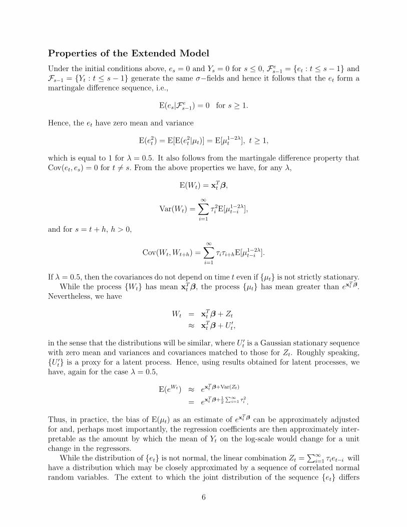
Properties of the Extended Model

Under the initial conditions above, es = 0 and Ys = 0 for s ≤ 0, F es−1 = et : t ≤ s− 1 and

Fs−1 = Yt : t ≤ s − 1 generate the same σ−fields and hence it follows that the et form amartingale difference sequence, i.e.,

E(es|F es−1) = 0 for s ≥ 1.

Hence, the et have zero mean and variance

E(e2t ) = E[E(e2t |µt)] = E[µ1−2λt ], t ≥ 1,

which is equal to 1 for λ = 0.5. It also follows from the martingale difference property thatCov(et, es) = 0 for t = s. From the above properties we have, for any λ,

E(Wt) = xTt β,

Var(Wt) =∞∑i=1

τ 2i E[µ

1−2λt−i ],

and for s = t+ h, h > 0,

Cov(Wt,Wt+h) =∞∑i=1

τiτi+hE[µ1−2λt−i ].

If λ = 0.5, then the covariances do not depend on time t even if µt is not strictly stationary.While the process Wt has mean xTt β, the process µt has mean greater than ex

Tt β.

Nevertheless, we have

Wt = xTt β + Zt

≈ xTt β + U ′t ,

in the sense that the distributions will be similar, where U ′t is a Gaussian stationary sequence

with zero mean and variances and covariances matched to those for Zt. Roughly speaking,U ′

t is a proxy for a latent process. Hence, using results obtained for latent processes, wehave, again for the case λ = 0.5,

E(eWt) ≈ exTt β+Var(Zt)

= exTt β+1

2

∑∞i=1 τ

2i .

Thus, in practice, the bias of E(µt) as an estimate of exTt β can be approximately adjusted

for and, perhaps most importantly, the regression coefficients are then approximately inter-pretable as the amount by which the mean of Yt on the log-scale would change for a unitchange in the regressors.

While the distribution of et is not normal, the linear combination Zt =∑∞

i=1 τiet−i willhave a distribution which may be closely approximated by a sequence of correlated normalrandom variables. The extent to which the joint distribution of the sequence et differs

6

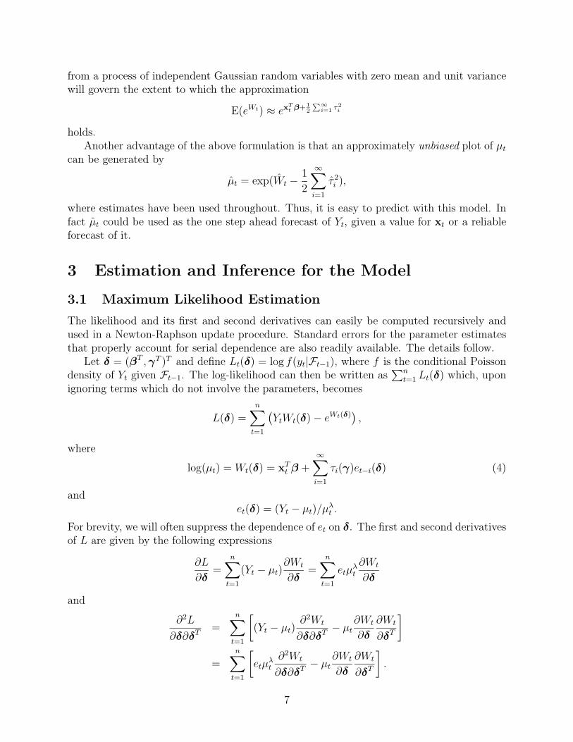
from a process of independent Gaussian random variables with zero mean and unit variancewill govern the extent to which the approximation

E(eWt) ≈ exTt β+1

2

∑∞i=1 τ

2i

holds.Another advantage of the above formulation is that an approximately unbiased plot of µt

can be generated by

µt = exp(Wt − 1

2

∞∑i=1

τ 2i ),

where estimates have been used throughout. Thus, it is easy to predict with this model. Infact µt could be used as the one step ahead forecast of Yt, given a value for xt or a reliableforecast of it.

3 Estimation and Inference for the Model

3.1 Maximum Likelihood Estimation

The likelihood and its first and second derivatives can easily be computed recursively andused in a Newton-Raphson update procedure. Standard errors for the parameter estimatesthat properly account for serial dependence are also readily available. The details follow.

Let δ = (βT ,γT )T and define Lt(δ) = log f(yt|Ft−1), where f is the conditional Poissondensity of Yt given Ft−1. The log-likelihood can then be written as

∑nt=1 Lt(δ) which, upon

ignoring terms which do not involve the parameters, becomes

L(δ) =n∑t=1

(YtWt(δ)− eWt(δ)

),

where

log(µt) = Wt(δ) = xTt β +

∞∑i=1

τi(γ)et−i(δ) (4)

andet(δ) = (Yt − µt)/µλt .

For brevity, we will often suppress the dependence of et on δ. The first and second derivativesof L are given by the following expressions

∂L

∂δ=

n∑t=1

(Yt − µt)∂Wt

∂δ=

n∑t=1

etµλt

∂Wt

∂δ

and

∂2L

∂δ∂δT=

n∑t=1

[(Yt − µt) ∂

2Wt

∂δ∂δT− µt∂Wt

∂δ

∂Wt

∂δT

]

=n∑t=1

[etµ

λt

∂2Wt

∂δ∂δT− µt∂Wt

∂δ

∂Wt

∂δT

].

7

The remaining expressions needed to calculate these derivatives are given in Appendix 5.2.Asymptotic results for these estimates are given in Appendix 5.3 for the basic model withλ = 1, p = 1 and xtβ = β. In this case, the asymptotic distribution of the maximumlikelihood estimates is N(0, V −1), where

V = limn→∞

1

n

n∑t=1

eWt(δ0)WtWTt , (5)

with Wt =∂Wt(δ0)

∂δ.

To initialize the Newton Raphson recursions we have found that using the GLM estimateswithout the autoregressive moving average terms together with zero initial values for et, t ≤0, gives reasonable starting values. Convergence in the majority of cases reported below(in which the first derivatives were less than 10−6) occurred within 10 iterations from thesestarting conditions. The covariance matrix of the estimators is estimated by

Ω = −(∂2L(θ)

∂δ∂δT

)−1

(6)

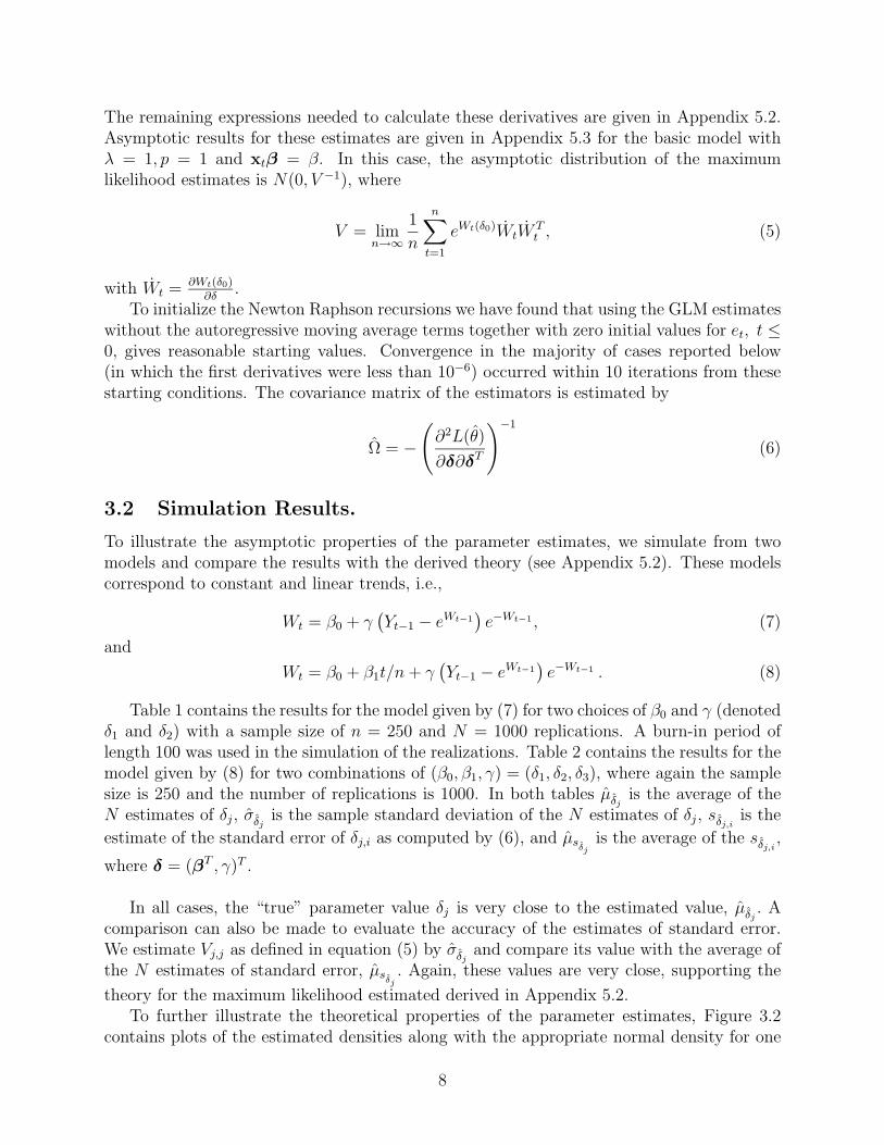
3.2 Simulation Results.

To illustrate the asymptotic properties of the parameter estimates, we simulate from twomodels and compare the results with the derived theory (see Appendix 5.2). These modelscorrespond to constant and linear trends, i.e.,

Wt = β0 + γ(Yt−1 − eWt−1

)e−Wt−1 , (7)

and

Wt = β0 + β1t/n+ γ(Yt−1 − eWt−1

)e−Wt−1 . (8)

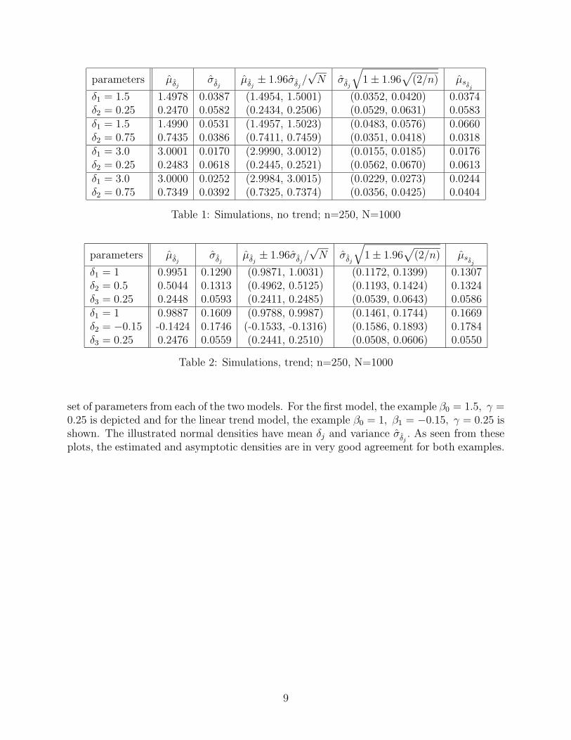
Table 1 contains the results for the model given by (7) for two choices of β0 and γ (denotedδ1 and δ2) with a sample size of n = 250 and N = 1000 replications. A burn-in period oflength 100 was used in the simulation of the realizations. Table 2 contains the results for themodel given by (8) for two combinations of (β0, β1, γ) = (δ1, δ2, δ3), where again the samplesize is 250 and the number of replications is 1000. In both tables µδj is the average of theN estimates of δj, σδj is the sample standard deviation of the N estimates of δj, sδj,i

is the

estimate of the standard error of δj,i as computed by (6), and µsδjis the average of the sδj,i

,

where δ = (βT , γ)T .

In all cases, the “true” parameter value δj is very close to the estimated value, µδj . Acomparison can also be made to evaluate the accuracy of the estimates of standard error.We estimate Vj,j as defined in equation (5) by σδj and compare its value with the average ofthe N estimates of standard error, µsδj

. Again, these values are very close, supporting the

theory for the maximum likelihood estimated derived in Appendix 5.2.To further illustrate the theoretical properties of the parameter estimates, Figure 3.2

contains plots of the estimated densities along with the appropriate normal density for one

8

parameters µδj σδj µδj ± 1.96σδj/√N σδj

√1± 1.96

√(2/n) µsδj

δ1 = 1.5 1.4978 0.0387 (1.4954, 1.5001) (0.0352, 0.0420) 0.0374δ2 = 0.25 0.2470 0.0582 (0.2434, 0.2506) (0.0529, 0.0631) 0.0583δ1 = 1.5 1.4990 0.0531 (1.4957, 1.5023) (0.0483, 0.0576) 0.0660δ2 = 0.75 0.7435 0.0386 (0.7411, 0.7459) (0.0351, 0.0418) 0.0318δ1 = 3.0 3.0001 0.0170 (2.9990, 3.0012) (0.0155, 0.0185) 0.0176δ2 = 0.25 0.2483 0.0618 (0.2445, 0.2521) (0.0562, 0.0670) 0.0613δ1 = 3.0 3.0000 0.0252 (2.9984, 3.0015) (0.0229, 0.0273) 0.0244δ2 = 0.75 0.7349 0.0392 (0.7325, 0.7374) (0.0356, 0.0425) 0.0404

Table 1: Simulations, no trend; n=250, N=1000

parameters µδj σδj µδj ± 1.96σδj/√N σδj

√1± 1.96

√(2/n) µsδj

δ1 = 1 0.9951 0.1290 (0.9871, 1.0031) (0.1172, 0.1399) 0.1307δ2 = 0.5 0.5044 0.1313 (0.4962, 0.5125) (0.1193, 0.1424) 0.1324δ3 = 0.25 0.2448 0.0593 (0.2411, 0.2485) (0.0539, 0.0643) 0.0586δ1 = 1 0.9887 0.1609 (0.9788, 0.9987) (0.1461, 0.1744) 0.1669δ2 = −0.15 -0.1424 0.1746 (-0.1533, -0.1316) (0.1586, 0.1893) 0.1784δ3 = 0.25 0.2476 0.0559 (0.2441, 0.2510) (0.0508, 0.0606) 0.0550

Table 2: Simulations, trend; n=250, N=1000

set of parameters from each of the two models. For the first model, the example β0 = 1.5, γ =0.25 is depicted and for the linear trend model, the example β0 = 1, β1 = −0.15, γ = 0.25 isshown. The illustrated normal densities have mean δj and variance σδj . As seen from theseplots, the estimated and asymptotic densities are in very good agreement for both examples.

9

1.40 1.45 1.50 1.55 1.60

02

46

81

0

0.10 0.15 0.20 0.25 0.30 0.35 0.40

01

23

45

67

Model (7), β0 = 1.5 Model (7), γ = 0.25

0.6 0.8 1.0 1.2 1.4

0.0

0.5

1.0

1.5

2.0

2.5

−0.6 −0.4 −0.2 0.0 0.2 0.4

0.0

0.5

1.0

1.5

2.0

2.5

Model (8), β0 = 1 Model (8), β1 = −0.15

0.10 0.15 0.20 0.25 0.30 0.35 0.40

01

23

45

67

Model (8), γ = 0.25

10

4 Applications.

4.1 Review of Previous Examples.

Davis et al. (1999) analyze the polio data introduced by Zeger (1988) using various GLARMAmodels. A summary of other analyses, including those based on parameter driven models,is also given by Davis et al. (1999). In addition, they analyze the UK sudden infant deathsyndrome series considered by Campbell (1994). Using a GLARMA model and other teststatistics for serial dependence in count time series they conclude that the serial dependenceeffects are not required, so that p = q = 0 in the GLARMA model. This conclusion hasrecently been confirmed by Jung and Liesenfeld (2001) using an approximation to maximumlikelihood estimation in a parameter driven model.

Davis et al. (1999, 2000) also report on a preliminary analysis of a series of daily countsof patients presenting at the accident and emergency department of Campbelltown Hospitallocated in the southwest metropolitan area of Sydney, Australia. Here we extend thatanalysis with a more comprehensive model for the seasonal effects and the pollution series.This results in a reasonably large number of covariates. This is one of several hospitals wheresimilar analyses can be performed and serves as an illustrative example for which we believethat the use of observation driven models is particularly well suited.

The analysis to be presented here modifies and extends the model considered for theCampbelltown asthma series in Davis et al. (1999). This previous model included explana-tory variables for a Sunday effect, a Monday effect, an increasing linear trend in timeand a seasonal pattern. The latter was modeled using Fourier series terms consisting ofcos(2πkt/365) and sin(2πkt/365) for k = 1, 2, 3, 4. To model the remaining serial dependencea GLARMA model with nonzero coefficients at lags 1,3,7 and 10 for the AR component andno moving average component was used. After fitting the model with these terms someslight overdispersion not explained by the lagged AR component of this observation drivenmodel remained. This points to the need for additional covariates or possibly a more flexibleseasonal pattern as well as a more complex serial dependence structure.

4.2 Analysis of Sydney Asthma Time Series.

The GLARMA model fit in Davis et al. (1999) did not address a major practical question forwhich the data was originally collected. Of interest was the role of air pollution levels on thenumber of daily asthma cases. Because meteorological conditions can be expected to playan important role in the pollution process, temperature can have a direct effect on asthmaoccurrences, and, because the growth of fungal spores and dust mite level can be relatedto humidity and temperature, it is reasonable to also consider inclusion of meteorologicalvariables in the model. See Samet et al. (1998) for a discussion of the potential for mete-orological conditions to play a role here. At the time of the analysis in Davis et al (1999),only partial data was available on relevant pollution series. Most importantly a series onparticulate levels had not been compiled. We now describe in detail the terms investigatedin the model and the sources of appropriate data.

11

4.2.1 Pollution measurements.

The New South Wales EPA provided all available pollution measurements for the Sydneymetropolitan region commencing prior to January 1, 1990 (the date at which the asthmadata commenced) and up to 1999. Unfortunately, for the time period of our data the networkcoverage was rather sparse for the southwest region of Sydney. After analyzing all availablerecords for completeness we selected the observations from the Lidcombe observing site forozone and NO2 measurements. Lidcombe is to the northeast of Campbelltown but wasconsidered to be sufficiently close so as to give representative readings for these pollutants.The other hospitals we analyzed were at Liverpool and Lidcome and are located even closer tothe Lidcombe station. Unfortunately, nepholometer readings of particulate concentrationswere not available at Lidcombe during the relevant time period. The two most completerecords were at Rozelle and Kensington both of which are considerably closer to downtownSydney and closer to the coastline. Particulate readings from these two locations wereaveraged to produce a single series. In addition, two types of pollution series were used:daily average and daily maximum readings based on hourly measurements.

4.2.2 Meteorological Data.

Meteorological data was obtained from the Australian Bureau of Meteorology at Liverpooland was considered to be relevant to the three hospitals considered. While there is spatialvariability in meteorological conditions across the Sydney basin the temporal variability (ofmost relevance to this analysis) is substantially larger and so using a single representativelocation for these data is reasonable. We were particularly interested in the effects of moistureon asthma levels. In exploratory analysis rainfall did not appear to play a major role, whereashumidity did with an approximate lag of 14 days. Details of the construction and statisticalsignificance of this variable are provided in Davis et al. (2000).

4.2.3 Seasonal Effects

Figure 1 of Davis et al. (2000) shows evidence of a triple peak seasonal pattern in thetime series of hospital admission counts. In Davis et al. (1999, 2000) the seasonal variationwas modeled using a harmonic regression with several harmonics for the annual frequency.This model may not be appropriate because the intensity of seasonal peaks appears tovary considerably from year to year. In the analysis to follow we propose an alternativerepresentation of the seasonal behavior that allows us to test the constancy from year toyear.

The timing of the peaks appears to line up with the terms in the K-12 school year. Atthat time in Sydney there were four terms per year with the break between terms one andtwo occurring at varying times due to the timing of the Easter vacation. In the revisedseasonal model we assume that there is a broad annual seasonal pattern that is the same inall years and is modeled using annual harmonics cos(2πt/365) and sin(2πt/365). To modelthe peaks, we used a beta function as follows:

p(x) =1

B(a, b)(x)a(1− x)b, x ∈ [0, 1]

12

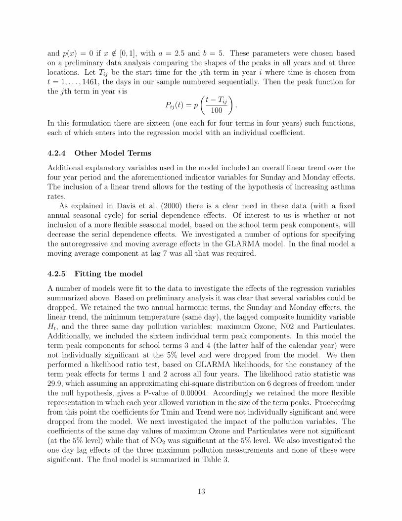
and p(x) = 0 if x /∈ [0, 1], with a = 2.5 and b = 5. These parameters were chosen basedon a preliminary data analysis comparing the shapes of the peaks in all years and at threelocations. Let Tij be the start time for the jth term in year i where time is chosen fromt = 1, . . . , 1461, the days in our sample numbered sequentially. Then the peak function forthe jth term in year i is

Pij(t) = p

(t− Tij100

).

In this formulation there are sixteen (one each for four terms in four years) such functions,each of which enters into the regression model with an individual coefficient.

4.2.4 Other Model Terms

Additional explanatory variables used in the model included an overall linear trend over thefour year period and the aforementioned indicator variables for Sunday and Monday effects.The inclusion of a linear trend allows for the testing of the hypothesis of increasing asthmarates.

As explained in Davis et al. (2000) there is a clear need in these data (with a fixedannual seasonal cycle) for serial dependence effects. Of interest to us is whether or notinclusion of a more flexible seasonal model, based on the school term peak components, willdecrease the serial dependence effects. We investigated a number of options for specifyingthe autoregressive and moving average effects in the GLARMA model. In the final model amoving average component at lag 7 was all that was required.

4.2.5 Fitting the model

A number of models were fit to the data to investigate the effects of the regression variablessummarized above. Based on preliminary analysis it was clear that several variables could bedropped. We retained the two annual harmonic terms, the Sunday and Monday effects, thelinear trend, the minimum temperature (same day), the lagged composite humidity variableHt, and the three same day pollution variables: maximum Ozone, N02 and Particulates.Additionally, we included the sixteen individual term peak components. In this model theterm peak components for school terms 3 and 4 (the latter half of the calendar year) werenot individually significant at the 5% level and were dropped from the model. We thenperformed a likelihood ratio test, based on GLARMA likelihoods, for the constancy of theterm peak effects for terms 1 and 2 across all four years. The likelihood ratio statistic was29.9, which assuming an approximating chi-square distribution on 6 degrees of freedom underthe null hypothesis, gives a P-value of 0.00004. Accordingly we retained the more flexiblerepresentation in which each year allowed variation in the size of the term peaks. Proceeedingfrom this point the coefficients for Tmin and Trend were not individually significant and weredropped from the model. We next investigated the impact of the pollution variables. Thecoefficients of the same day values of maximum Ozone and Particulates were not significant(at the 5% level) while that of NO2 was significant at the 5% level. We also investigated theone day lag effects of the three maximum pollution measurements and none of these weresignificant. The final model is summarized in Table 3.

13

Variable Coefficient S.E. T-ratioIntercept 0.583 0.062 9.46Sunday 0.197 0.056 3.53Monday 0.230 0.055 4.20Annual Cosine -0.214 0.039 -5.54Annual Sine 0.176 0.040 4.35Term 1, 1990 0.200 0.056 3.54Term 2, 1990 0.132 0.057 2.31Term 1, 1991 0.087 0.066 1.32Term 2, 1991 0.172 0.057 2.99Term 1, 1992 0.254 0.055 4.66Term 2, 1992 0.308 0.049 6.31Term 1, 1993 0.439 0.050 8.77Term 2, 1993 0.116 0.061 1.91Humidity Ht/20 0.169 0.055 3.09NO2 max -0.104 0.033 -3.16MA, lag 7 0.042 0.018 2.32

Table 3: Analysis of Sydney Asthma Time Series

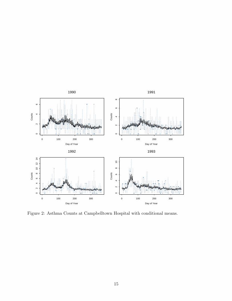
The fitted values from the model are shown in Figure 2 along with the actual counts. In thisfinal model, various test statistics reviewed in Davis et al. (1999, 2000) for the presence of alatent process and the degree of autocorrelation indicated that there was no need to includeadditional autoregressive or moving average terms.

4.2.6 Discussion

The expanded and revised model for the Campbelltown asthma series allows for seasonalpatterns to be aligned with the school term dates and to vary in intensity from year to year.These differences are highly statistically significant. Virally induced asthma occurrencesmight be synchronized in part with the school terms and would not necessarily occur withthe same intensity in the same terms across different years or across terms in the same year.

The use of a more flexible seasonal model leads to a simplification of the lag dependencestructure compared with that in previous analyses. However, moving average dependenceat lag 7 is positive and significant. Inferences about the key pollution and weather variablesare adjusted for this serial dependence in the above analysis.

The same analysis was repeated at two other locations: Liverpool and Lidcome hospitals.Similar results were obtained for these two sites. However, at these places none of thepollution variables were statistically significant.

5 Appendix

This section provides theoretical complements to Sections 2 and 3. In particular, we estab-lish existence of stationary solutions to the GLARMA model and give a derivation for the

14

1990

Day of Year

Cou

nts

0 100 200 300

02

46

1991

Day of Year

Cou

nts

0 100 200 300

02

46

8

1992

Day of Year

Cou

nts

0 100 200 300

02

46

810

1214

1993

Day of Year

Cou

nts

0 100 200 300

02

46

810

Figure 2: Asthma Counts at Campbelltown Hospital with conditional means.

15

asymptotic normality of maximum likelihood estimators in some reduced cases.

5.1 Existence of Stationary Solutions.

In this section, we establish the existence of a stationary solution for the process Wt underthe basic model with 1/2 ≤ λ ≤ 1 and xtβ = β given by,

Wt = β + γ(Yt−1 − eWt−1)e−λWt−1 . (9)

The result is first stated for a general Markov chain and then shown to hold for the processgiven by (9) with 1/2 ≤ λ ≤ 1.

Additionally, for the special case λ = 1, we will prove that the stationary distribution isunique using techniques from Meyn and Tweedie (1993). The remainder of this section isdivided into these two goals.

Existence: 1/2 ≤ λ ≤ 1.We begin by stating the existence results for a general Markov chain.

Proposition 5.1 If Xn is a weak Feller chain and if for any ε > 0 there exists a compactset C ⊂ X such that

P (x, Cc) < ε, for all x ∈ X,then Xn is bounded in probability; thus, there exists at least one stationary distribution forthe chain.

Proof: Assume that for any ε > 0 there exists a compact set C ⊂ X such that P (x, Cc) < εfor all x ∈ X. If P k(x, ·) denotes the k-step transition probability of the chain starting fromstate x then,

P k(x, Cc) =

∫P (y, Cc)P k−1(x, dy)

< ε.

Thus, the chain is bounded in probability. In fact, the tightness of the k-step transitionprobabilities holds uniformly in x. It follows that the chain is bounded in probability on av-erage and hence, by Theorem 12.0.1(i) of Meyn and Tweedie (1993), there exists a stationarydistribution.

Proposition 5.2 Let

Yt ∼ Poisson(eWt),

where

Wt = γ(Yt−1 − eWt−1)e−λWt−1 ,

1/2 ≤ λ ≤ 1. Then the chain is bounded in probability, and therefore, admits an invariantmeasure.

16

Proof: First note that the chain is weak Feller. Define C := [−c, c]. Then,P (x, Cc) = P (Wt ∈ Cc | Wt−1 = x)

= P[γ(Yt−1 − eWt−1

)e−λWt−1 ∈ [−c, c]c ∣∣ Wt−1 = x

],

which, by Markov’s inequality,

≤

(γ/c)2e−2λxVar[Yt | Wt−1 = x

], x ≥ 0

(γ/c)e−λxE[∣∣Yt−1 − ex

∣∣ ∣∣ Wt−1 = x], x < 0

≤

(γ/c)2e(1−2λ)x, x ≥ 02(γ/c)e(1−λ)x, x < 0

≤

(γ/c)2, x ≥ 02(γ/c), x < 0.

Thus, given ε > 0 choose c large such that max(2(γ/c), (γ/c)2

)< ε. The result follows from

Proposition 5.1.

Uniqueness: λ = 1.Under this assumption on λ, we are able to establish uniqueness of the stationary distri-bution. To accomplish this we shall show that the process Wt is aperiodic and satisfiesDoeblin’s condition. It then follows from Theorem 16.2.3 of Meyn and Tweedie (1993) thatWt is uniformly ergodic. We first begin with a statement of Doeblin’s condition:

There exists a probability measure ν with the property that for some m ≥ 1, ε > 0, andδ > 0

ν(B) > ε =⇒ Pm(x,B) ≥ δ, (10)

for every x ∈ X.

Proposition 5.3 The process Wt given in equation (9) satisfies Doeblin’s condition andis strongly aperiodic. Hence, the process is uniformly ergodic.

Proof: In order to establish Doeblin’s Condition, we consider the two cases γ < 0 and γ > 0.Case 1: γ < 0¿From (9) with λ = 1, one can see thatWt = β−γ+γYt−1e

Wt−1 ≤ β−γ. Define the measureν to have unit point mass at β − γ. In order to verify (10), it suffices to only considerBorel sets B with β − γ ∈ B. Then, for all x ≤ β − γ,

P (x,B) = P (Wt ∈ B | Wt−1 = x)

≥ P (Wt = β − γ | Wt−1 = x)

= P (Yt−1 = 0 | Wt−1 = x)

= e−ex

≥ e−eβ−γ

,

which yields (10) with m = 1.Case 2: γ > 0For γ > 0, Wt has a lower bound of β − γ and hence, the state space for Wt is a subset of

17

[β − γ,∞). As in Case 1, we will take the measure ν to have unit mass at β − γ. LetC = [β − γ,max(ε, β + γ)], where ε > 0. Then, for all x ∈ C and Borel sets B containingβ − γ,

P (x,B) = P (Wt ∈ B | Wt−1 = x)

≥ P (Wt = β − γ | Wt−1 = x)

= P (Yt−1 = 0 | Wt−1 = x)

= e−ex

≥ e−emax(ε,β+γ)

:= δ1,

and

P 2(x,B) ≥ P (Wt+1 = β − γ,Wt = β − γ | Wt−1 = x)

≥ δ21.

On the other hand if x /∈ C, then x > max(ε, β + γ) and we have

P (x,C) = P (Wt ∈ C | Wt−1 = x)

≥ P (β − γ ≤ Wt ≤ β + γ | Wt−1 = x)

= P (|Wt − β| ≤ γ | Wt−1 = x)

≥ 1− γ−2V ar (Wt | Wt−1 = x) (by Chebyshev’s Inequality)

= 1− γ−2γ2e−x

≥ 1− e−max(ε,β+γ) := δ2.

Therefore,

P 2(x,B) = P (Wt ∈ B | Wt−2 = x)

≥ P (Wt ∈ B,Wt−1 ∈ C | Wt−2 = x)

=∑y∈C

P (Wt ∈ B,Wt−1 = y | Wt−2 = x)

=∑y∈C

P (Wt ∈ B | Wt−1 = y)P (Wt−1 = y | Wt−2 = x)

≥ δ1P (Wt−1 ∈ C | Wt−2 = x)

≥ δ1δ2.

Thus, Doeblin’s condition is also satisfied for the case γ ∈ (0, 1].For both cases, i.e., 0 < |γ| ≤ 1, the chain Wt is also strongly aperiodic since

P (β − γ, β − γ) = P (Wt = β − γ | Wt−1 = β − γ)= P (Yt−1 = 0 | Wt−1 = β − γ)= e−e

β−γ

> 0.

As remarked earlier, we conclude that Wt must be uniformly ergodic.

18

The result given above for λ = 1 extends to the case

Wt = β +

p∑i=1

γi(Yt−i − eWt−i)e−Wt−i

by considering the p−variate Markov chain (Wt,Wt−1, . . .Wt−p+1).

5.2 Maximum Likelihood Calculations

In this section, we derive the remaining expressions needed for the maximum likelihoodcalculations of Section 3.1. Recall,

∂L

∂δ=

n∑t=1

(Yt − µt)∂Wt

∂δ=

n∑t=1

etµλt

∂Wt

∂δ,

and∂2L

∂δ∂δT=

n∑t=1

[etµ

λt

∂2Wt

∂δ∂δT− µt∂Wt

∂δ

∂Wt

∂δT

].

First we note that∂et∂δ

= −[e(1−λ)Wt + λet]∂Wt

∂δ.

Also∂Wt

∂δ= xTt

∂β

∂δ+∂Zt∂δ,

where

Zt =∞∑i=1

τiet−i

= (φ(B)−1θ(B)− 1)et,

so that

Zt =

p∑i=1

φi(Zt−i + et−i) +q∑i=1

θiet−i.

It follows that

∂Zt∂δ

=

p∑i=1

∂φi∂δ

(Zt−i + et−i) +p∑i=1

φi

(∂Zt−i∂δ

+∂et−i∂δ

)

+

q∑i=1

∂θi∂δet−i +

q∑i=1

θi∂et−i∂δ

.

In particular:

∂Zt∂βa

=

p∑i=1

φi

(∂Zt−i∂βa

+∂et−i∂βa

)+

q∑i=1

θi∂et−i∂βa

,

19

∂Zt∂φa

= Zt−a + et−a +p∑i=1

φi

(∂Zt−i∂φa

+∂et−i∂φa

)+

q∑i=1

θi∂et−i∂φa

and∂Zt∂θa

=

p∑i=1

φi

(∂Zt−i∂θa

+∂et−i∂θa

)+ et−a +

q∑i=1

θi∂et−i∂θa

.

The second derivatives are then

∂2et

∂δ∂δT= −[e(1−λ)Wt + λet]

∂2Wt

∂δ∂δT

−[∂Wt

∂δ(1− λ)e(1−λ)Wt + λ

∂et∂δ

]∂Wt

∂δT

and∂2Wt

∂δ∂δT=∂2βT

∂δ∂δTxt +

∂δ2Zt

∂δ∂δT=∂δ2Zt

∂δ∂δT,

in which

∂2Zt

∂δ∂δT=

p∑i=1

[∂φi∂δ

(∂Zt−i∂δT

+∂et−i∂δT

)+

(∂Zt−i∂δ

+∂et−i∂δ

)∂φi

∂δT

]

+

p∑i=1

φi

(∂2Zt−i∂δ∂δT

+∂2et−i∂δ∂δT

)+

q∑i=1

[∂θi∂δ

∂et−i∂δT

+∂et−i∂δ

∂θi

∂δT

]

+

q∑i=1

θi∂2et−i∂δ∂δT

.

5.3 Asymptotic Distribution of MLE

In this section we establish asymptotic properties of the MLEs given in Section 3.1 for thespecific case of the basic model with λ = 1, p = 1 and xTt β = β. Uniform ergodicity(as established in Proposition 5.3) and stationarity of Wt are the key ingredients of theargument.

First replace Wt(δ) by

W †t (δ) = Wt(δ0) + (δ − δ0)

T Wt,

where Wt =∂Wt(δ0)

∂δand define a linearized form of the likelihood as

L†(δ) =n∑t=1

(YtW

†t (δ)− eW

†t (δ)

).

Unless otherwise indicated, Wt and Wt are evaluated at δ0. Now, re-parameterizing with

20

the transformation u = n1/2(δ − δ0), we have

R†n(u) := L†(δ0)− L†(δ0 + un

−1/2)

= −uTn−1/2

n∑t=1

YtWt +n∑t=1

eWt

(eu

Tn−1/2Wt − 1)

= −uTn−1/2

n∑t=1

(Yt − eWt

)Wt +

n∑t=1

eWt

(eu

Tn−1/2Wt − 1− uTn−1/2Wt

). (11)

Note that R†n(u) is a convex function of u. The first term in (11) can be written as

−uTHn where

Hn := n−1/2

n∑t=1

eteWtWt

and et =(Yt − eWt

)/eWt . Now this is a sum of a triangular array of vector martingale

differencesηnt = n

−1/2etbt,

wherebt = Wte

Wt = Wtµt.

In order to apply a martingale central limit theorem, it suffices to show (see Corollary 3.1 ofHall and Heyde [8]) that

n∑t=1

E(ηntηTnt | Ft−1)

P−→ V (δ0), (12)

where Ft = σ(Ys, s ≤ t), and, for all ε > 0,

n∑t=1

E(ηntη

TntI(|ηnt| > ε) | Ft−1

) P−→ 0. (13)

We then haveHn

d→ N(0, V ),

where

V = limn→∞

1

n

n∑t=1

∂Lt(δ0)

∂δ

∂Lt(δ0)

∂δT= lim

n→∞1

n

n∑t=1

e2t e2WtWtW

Tt .

The second term in (11) is

uT

[(2n)−1

n∑t=1

eWtWtWTt

]u+Op

(n−3/2

n∑t=1

eWt(uT Wt)3

)

in which the second term converges to zero. Hence

R†n(u)

d→ R(u) := −uTN(0, V ) + uTV u/2,

21

where

V = limn→∞

1

n

n∑t=1

eWtWtWTt .

It then follows that u†n =argminR†n(u)

d→ u =argminR(u). From the form of R(u), we seethat u = V −1N(0, V ) ∼ N(0, V −1).

Next, we pass the convergence of R†n(u) onto Rn(u) := L(δ0)−L(un−1/2+δ0). Specifically,

it suffices to show that L(un−1/2 +δ0)−L†(un−1/2 +δ0)P→ 0 uniformly for |u| ≤ K.Writing

δ = un1/2 + δ0, we have

L(δ)− L†(δ)

=n∑t=1

YtWt(δ)−n∑t=1

eWt(δ) −n∑t=1

Yt

(Wt + u

Tn−1/2Wt

)+

n∑t=1

eWt+uTn−1/2Wt

=n∑t=1

Yt

(Wt(δ)−Wt − uTn−1/2Wt

)−

n∑t=1

(eWt(δ) − eWt+uTn−1/2Wt

)

=n∑t=1

(Yt − eWt

) (Wt(δ)−Wt − uTn−1/2Wt

)

−n∑t=1

[eWt(δ) − eWt+uTn−1/2Wt − eWt

(Wt(δ)−Wt − uTn−1/2Wt

)]. (14)

The first term in equation (14) is

An =n∑t=1

(Yt − eWt

) (Wt(δ)−Wt − uTn−1/2Wt

)

= uT (2n)−1

[n∑t=1

(Yt − eWt

)Wt +

n∑t=1

(Yt − eWt

) (Wt(δ

∗)− Wt

)]u.

Since (Yt − eWt)Wt is stationary and E[(Yt − eWt)Wt] = 0, An → 0 uniformly for |u| ≤ K

and for all K < ∞, where ‖δ∗ − δ0‖ ≤ ‖δ − δ0‖ assuming Wt(δ∗) − Wt

P→ 0. The secondterm is

Bn = −n∑t=1

[eWt(δ) − eWt+uTn−1/2Wt − eWt

(Wt(δ)−Wt − uTn−1/2Wt

)],

22

which after expanding eWt(δ), euTn−1/2Wt and Wt(δ) in a Taylor series is

= −n∑t=1

[eWt + uTn−1/2eWtWt + u

T (2n)−1eWt(δ∗1)

(W 2

t (δ∗1) + Wt(δ

∗1)

)u

−eWt

(1 + uTn−1/2Wt + e

c(2n)−1uT W 2t u

)−eWt

(Wt + u

Tn−1/2Wt + uT (2n)−1Wt(δ

∗2)u−Wt − uTn−1/2Wt

)]

= −uT (2n)−1

n∑t=1

(eWt(δ

∗1) − eWt

) (W 2

t (δ∗1) + Wt(δ

∗1)

)

+n∑t=1

eWt

[(W 2

t (δ∗1)− ecW 2

t

)+

(Wt(δ

∗1)− Wt(δ

∗2)

)]u,

where 0 ≤ c ≤ uT

2nWt(δ0) and

∥∥δ∗j − δ0

∥∥ ≤ ‖δ − δ0‖ for j = 1, 2. Assuming each averagein the above expression converges to a finite quantity in probability, we have that Bn → 0

uniformly on compact subsets for u. Therefore, L(δ)−L†(δ) P→ 0 uniformly for |u| ≤ K, forall K <∞ and we obtain the desired result:

Rn(u)d→ R(u) := −uTN(0, V ) + uTV u/2.

We now consider establishing conditions (12) and (13). ¿From (9) we see that

Wt =

[ ∂Wt

∂γ∂Wt

∂β

]=

[Wt,1

Wt,2

]

=

[Yt−1e

−Wt−1 − 1− γYt−1e−Wt−1Wt−1,1

1− γyt−1e−Wt−1Wt−1,2

]

=

[Ut + AtWt−1,1

1 + AtWt−1,2

]=

[Ut +

∑∞i=1At · · ·At−i+1Ut−i

1 +∑∞

i=1At · · ·At−i+1

], (15)

where Ut = Yt−1e−Wt−1 − 1 and At = −γYt−1e

−Wt−1 . Since Wt is a function of Ws, s ≤ t,it also is a strictly stationary ergodic process. Now,

n∑t=1

E(ηntηTnt | Ft−1) =

1

n

n∑t=1

eWtWtWTt ,

which is a function of two stationary ergodic processes, Wt and Wt. By the ergodictheorem we then have

1

n

n∑t=1

eWtWtWTt

a.s.−→ V = E(eW1W1WT1 )

if E|eWt(δ0)WtWTt | < ∞. Conditions under which this holds will now be derived for a

particular choice of parameter values of β and γ. It suffices to show E|eWtW 2t,i| <∞, i = 1, 2.

First we will consider the case i = 1. Using ‖ · ‖2 to denote the L2 norm, we have from (15),

‖eWt/2Wt,1‖2 ≤ ‖eWt/2Ut‖2 +∞∑i=1

‖eWt/2At · · ·At−i+1Ut−i‖2.

23

Using properties of the moment generating function for a Poisson distributed random variableand the fact that the process Wt is bounded below by β − γ, we have

‖eWt/2Ut‖22 = E

[eβ−γeγYt−1e

−Wt−1(Yt−1e

−Wt−1 − 1)2]

= eβ−γE[E

(eγYt−1e

−Wt−1(Y 2

t−1e−2Wt−1 − 2Yt−1e

−Wt−1 + 1) | Wt−1

)]= eβ−γE

[e−Wt−1eγe

−Wt−1ee

Wt−1 (eγe−Wt−1−1) + e2γe

−Wt−1ee

Wt−1 (eγe−Wt−1−1)

−2eγe−Wt−1

eeWt−1 (eγe

−Wt−1−1) + eeWt−1 (eγe

−Wt−1−1)

]

= eβ−γE[ee

Wt−1 (eγe−Wt−1−1)

[1 + eγe

−Wt−1(eγe

−Wt−1+ e−Wt−1 − 2

)]]

≤ eβ−γeeβ−γ(eγe−(β−γ)−1)

[1 + eγe

−(β−γ)(eγe

−(β−γ)

+ e−(β−γ) − 2)]

:= c21,

E[eWtA2

t | Ft−1

]= E

[γ2eβ−γY 2

t−1e−2Wt−1eγYt−1e

−Wt−1 | Wt−1

]= γ2eβ−γ

[e−Wt−1eγe

−Wt−1ee

Wt−1 (eγe−Wt−1−1) + e2γe

−Wt−1ee

Wt−1 (eγe−Wt−1−1)

]

≤ γ2eβ−γeeβ−γ(eγe−(β−γ)−1)eγe

−(β−γ)(eγe

−(β−γ)

+ e−(β−γ)):= b21,

E[A2t | Ft−1

]= E

[γ2Y 2

t−1e−2Wt−1 | Wt−1

]= γ2

(1 + e−Wt−1

)≤ γ2(1 + e−(β−γ))

andE

[U2t | Ft−1

]= E

[Y 2t−1e

−2Wt−1 − 2Yt−1e−Wt−1 + 1 | Wt−1

]= e−Wt−1

≤ e−(β−γ) := b22.

Applying these results, ‖eWt/2At · · ·At−i+1Ut−i‖22 may be calculated recursively:

‖eWt/2At · · ·At−i+1Ut−i‖22 = E

(eWtA2

t · · ·A2t−i+1U

2t−i

)= E

[E

(eWtA2

t · · ·A2t−i+1U

2t−i | Ft−1

)]= E

[A2t−1 · · ·A2

t−i+1U2t−iE

(eWtA2

t | Ft−1

)]≤ b21E

[E

(A2t−1 · · ·A2

t−i+1U2t−i | Ft−2

)]= b21E

[A2t−2 · · ·A2

t−i+1U2t−iE

(A2t−1 | Ft−2

)]≤ b21γ

2(1 + e−(β−γ))E[A2t−2 · · ·A2

t−i+1U2t−i

]...

≤ b21(γ2(1 + e−(β−γ))

)i−1E [E (Ut−i | Ft−i−1)]

≤ b21b22

(γ2(1 + e−(β−γ))

)i−1.

24

Therefore,

‖eWt/2Wt,1‖2 ≤ c1 + c2∞∑i=1

γi−1(1 + eγ−β)(i−1)/2,

where c2 = b1b2.

Likewise,

‖eWt/2Wt,2‖2 ≤ ‖eWt/2‖2 +∞∑i=0

‖eWt/2At · · ·At−i‖2

≤ c3 + c4

∞∑i=1

γi−1(1 + eγ−β)(i−1)/2,

where c3 =[eβ−γee

β−γ(eγe−(β−γ)−1)]1/2

and c4 =[γ2eβ−γee

β−γ(eγe−(β−γ)−1)eγe−(β−γ)

(eγe

−(β−γ)+ e−(β−γ)

)]1/2

.

Therefore, E|eWtWtWTt | will be finite for γ(1 + eγ−β)1/2 < 1.

The convergence required in condition (13) is easily established using condition (12) andthe stationarity of Wt. Now,

n∑t=1

E(ηntη

TntI(|ηnt > ε)||Ft−1

)

=1

n

n∑t=1

E[(Yt−1 − eWt−1)2WtW

Tt I(|(Yt−1 − eWt−1)Wt| > ε

√n)|Ft−1

]

≤ 1

n

n∑t=1

E[(Yt−1 − eWt−1)2WtW

Tt I(|(Yt−1 − eWt−1)Wt| > M)|Ft−1

]n→∞−→ E

[(Y1 − eW1)2W1W

T1 I(|(Y1 − eW1)W1| > M)

]−→ 0 asM → ∞.

Therefore, the asymptotic distribution of the maximum likelihood estimates is N(0, V −1)where

V = limn→∞

1

n

n∑t=1

eWt(δ0)WtWTt .

References

[1] Campbell, M. J. (1994) “Time series regression for counts: an investigation into therelationship between sudden infant death syndrome and environmental temperature”, J.R. Statist. Soc. A, 157, 191-208.

[2] Cox, D.R. (1981). “Statistical Analysis of Time Series: Some Recent Developments.”Scandinavian Journal of Statistics, 8, 93–115.

25

[3] Davis, R.A., Dunsmuir, W.T.M., and Wang, Y. (1999). “Modelling Time Series of CountData.” Asymptotics, Nonparametrics, and Time Series (Subir Ghosh, editor) Marcel-Dekker, New York, 63–114.

[4] Davis, R.A., Dunsmuir, W.T.M., and Wang, Y. (2000). “On Autocorrelation in a PoissonRegression Model” (with W.T.M. Dunsmuir and Y. Wang). Biometrika 87 491–506.

[5] Diggle, P.J., K-Y Liang and S.L. Zeger (1994) Analysis of Longitudinal Data, OxfordUniversity Press, Oxford.

[6] Durbin, J. and Koopman, S.J. (2000) “Time series analysis of non-Gaussian obser-vations based on state space models from both classical and Bayesain perspectives”,J. R. Statist. Soc. B 62, p3–56.

[7] Fahrmeir, L. and Tutz, G. (1994) Multivariate Statistical Modeling Based on GeneralisedLinear Models, Springer-Verlag, New York.

[8] Hall, P. and Heyde, C.C. (1980) “Martingale limit theory and its application”, AcademicPress, New York.

[9] Jung, R.C. and Liesenfeld, R. (2001). “Estimating time series models for count data usingefficient importance sampling.” (To appear in Allgemeines Statistisches Archive, 85.)

[10] Meyn, S.P. and Tweedie, R.L. (1994). “Markov Chains and Stochastic Stability”.Springer-Verlag, New York.

[11] Rydberg, T.H. and Shephard, N. (1999). “BIN models for trade-by-trade data. Mod-elling the number of trades in a fixed interval of time.” (Working paper, Oxford Univer-sity).

[12] Samet, J., Zeger, S., Kelsall, J., Xu, J., and Kalkstein, L. (1988). “Does weather con-found or modify the association of particulate air pollution with mortality? An analysisof the Philadelphia data, 1973-1980.” Environ Res 77;1: 9-19

[13] Shephard, Neil (1995) “Generalized Linear Autoregressions”. (Unpublished paper, Ox-ford University)

[14] Zeger, S. L. (1988) “A regression model for time series of counts”, Biometrika 75, 621-629.

[15] Zeger, S. L. and Qaqish, B. (1988) “Markov regression models for time series: a quasi-likelihood approach”, Biometrics 44, 1019-1031.

26