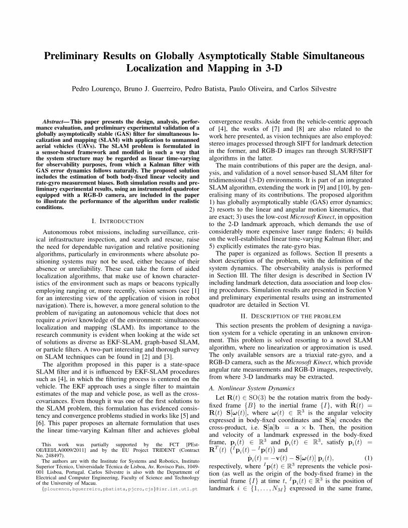
Preliminary Results on Globally Asymptotically Stable SimultaneousLocalization and Mapping in 3-D

Pedro Lourenco, Bruno J. Guerreiro, Pedro Batista, Paulo Oliveira, and Carlos Silvestre

Abstract— This paper presents the design, analysis, perfor-mance evaluation, and preliminary experimental validation of aglobally asymptotically stable (GAS) filter for simultaneous lo-calization and mapping (SLAM) with application to unmannedaerial vehicles (UAVs). The SLAM problem is formulated ina sensor-based framework and modified in such a way thatthe system structure may be regarded as linear time-varyingfor observability purposes, from which a Kalman filter withGAS error dynamics follows naturally. The proposed solutionincludes the estimation of both body-fixed linear velocity andrate-gyro measurement biases. Both simulation results and pre-liminary experimental results, using an instrumented quadrotorequipped with a RGB-D camera, are included in the paperto illustrate the performance of the algorithm under realisticconditions.

I. INTRODUCTION

Autonomous robot missions, including surveillance, crit-ical infrastructure inspection, and search and rescue, raisethe need for dependable navigation and relative positioningalgorithms, particularly in environments where absolute po-sitioning systems may not be used, either because of theirabsence or unreliability. These can take the form of aidedlocalization algorithms, that make use of known character-istics of the environment such as maps or beacons typicallyemploying ranging or, more recently, vision sensors (see [1]for an interesting view of the application of vision in robotnavigation). There is, however, a more general solution to theproblem of navigating an autonomous vehicle that does notrequire a priori knowledge of the environment: simultaneouslocalization and mapping (SLAM). Its importance to theresearch community is evident when looking at the wide setof solutions as diverse as EKF-SLAM, graph-based SLAM,or particle filters. A two-part interesting and thorough surveyon SLAM techniques can be found in [2] and [3].

The algorithm proposed in this paper is a state-spaceSLAM filter and it is influenced by EKF-SLAM proceduressuch as [4], in which the filtering process is centered on thevehicle. The EKF approach uses a single filter to maintainestimates of the map and vehicle pose, as well as the cross-covariances. Even though it was one of the first solutions tothe SLAM problem, this formulation has evidenced consis-tency and convergence problems studied in works like [5] and[6]. This paper proposes an alternate formulation that usesthe linear time-varying Kalman filter and achieves global

This work was partially supported by the FCT [PEst-OE/EEI/LA0009/2011] and by the EU Project TRIDENT (ContractNo. 248497).

The authors are with the Institute for Systems and Robotics, InstitutoSuperior Tecnico, Universidade Tecnica de Lisboa, Av. Rovisco Pais, 1049-001 Lisboa, Portugal. Carlos Silvestre is also with the Department ofElectrical and Computer Engineering, Faculty of Science and Technologyof the University of Macau.{plourenco,bguerreiro,pbatista,pjcro,cjs}@isr.ist.utl.pt

convergence results. Aside from the vehicle-centric approachof [4], the works of [7] and [8] are also related to thework here presented, as vision techniques are also employed:stereo images processed through SIFT for landmark detectionin the former, and RGB-D images ran through SURF/SIFTalgorithms in the latter.

The main contributions of this paper are the design, anal-ysis, and validation of a novel sensor-based SLAM filter fortridimensional (3-D) environments. It is part of an integratedSLAM algorithm, extending the work in [9] and [10], by gen-eralising many of its contributions. The proposed algorithm1) has globally asymptotically stable (GAS) error dynamics;2) resorts to the linear and angular motion kinematics, thatare exact; 3) uses the low-cost Microsoft Kinect, in oppositionto the 2-D landmark approach, which demands the use ofconsiderably more expensive laser range finders; 4) buildson the well-established linear time-varying Kalman filter; and5) explicitly estimates the rate-gyro bias.

The paper is organized as follows. Section II presents ashort description of the problem, with the definition of thesystem dynamics. The observability analysis is performedin Section III. The filter design is described in Section IVincluding landmark detection, data association and loop clos-ing procedures. Simulation results are presented in Section Vand preliminary experimental results using an instrumentedquadrotor are detailed in Section VI.

II. DESCRIPTION OF THE PROBLEM

This section presents the problem of designing a naviga-tion system for a vehicle operating in an unknown environ-ment. This problem is solved resorting to a novel SLAMalgorithm, where no linearization or approximation is used.The only available sensors are a triaxial rate-gyro, and aRGB-D camera, such as the Microsoft Kinect, which provideangular rate measurements and RGB-D images, respectively,from where 3-D landmarks may be extracted.

A. Nonlinear System DynamicsLet R(t) ∈ SO(3) be the rotation matrix from the body-

fixed frame {B} to the inertial frame {I}, with R(t) =R(t) S[ω(t)], where ω(t) ∈ R3 is the angular velocityexpressed in body-fixed coordinates and S[a] encodes thecross-product, i.e. S[a]b = a × b. Then, the positionand velocity of a landmark expressed in the body-fixedframe, pi(t) ∈ R3 and pi(t) ∈ R3, satisfy pi(t) =RT (t)

(Ipi(t)− Ip(t)

)and

pi(t) = −v(t)− S[ω(t)] pi(t), (1)respectively, where Ip(t) ∈ R3 represents the vehicle posi-tion (as well as the origin of the body-fixed frame) in theinertial frame {I} at time t, Ipi(t) ∈ R3 is the position oflandmark i ∈ {1, . . . , NM} expressed in the same frame,

and v(t) ∈ R3 denotes the velocity of the vehicle expressedin the body-fixed frame. Note that landmarks are assumedto be static in the inertial frame. It is important to noticethat ω(t) is available through noisy and biased rate-gyrosmeasurements ωm(t) = ω(t) + bω(t) + nω(t), where thebias bω(t) ∈ R3 is assumed constant and nω(t) ∈ R3

corresponds to the rate-gyro noise, which is assumed to bezero-mean white Gaussian noise with standard deviation σnω

in each component, i.e., nω(t) ∼ N(0, σ2nω

I3). Taking thisinto account, and using the cross product property a× b =−b× a, it is possible to rewrite (1) as

pi(t) = −v(t)− S[pi(t)] bω(t)− S[ωm(t)] pi(t). (2)

The vehicle-related variables, i.e., the linear velocity andthe angular measurement bias will constitute the vehiclestate, xV (t) :=

[vT (t) bTω (t)

]T ∈ RnV , with simpledynamics given by xV (t) = 0, which means that bothare assumed, in a deterministic setting, as constant. In thefiltering framework, the inclusion of state disturbances allowsto consider them as slowly time-varying.

It is now possible to derive the full state dynamics. Forthat purpose consider the position landmark dynamics (2),which may now be expressed as a function of the state vector,yielding

pi(t) = AMVi(pi(t)) xV (t)− S[ωm(t)]pi(t),

where AMVi(pi(t)) = [−I3 −S[pi(t)]] and In is the

identity matrix of dimension n. Finally, the NO observed,also designated as visible, landmarks xO(t) ∈ RnO

and the NU unobserved or non-visible ones xU (t) ∈RnU are concatenated in the landmark-based state vector,xM (t) :=

[xTO(t) xTU (t)

]T ∈ RnM . The two state vec-tors here defined constitute the full state vector xF (t) =[xTV (t) xTM (t)

]T, with the full system dynamics reading{

xF (t) = AF (t,xM (t))xF (t)

y(t) = xO(t), (3)

with

AF (t,xM (t)) =

[0nV

0nV ×nM

AMV (xM (t)) AM (t)

],

where

AMV (xM (t)) =[AT

MV1(p1(t)) · · · AT

MVNM(pNM

(t))]T

,

AM (t) = diag (−S[ωm(t)], · · · ,−S[ωm(t)]), and 0n×m isa n by m matrix filled with zeros and, if m is omitted, thematrix is square. From (3) it follows that the system maybe expressed in a way similar to the usual linear dynamicalsystem form. However, it is obvious to conclude that thesystem above is nonlinear, as the dynamics matrix dependson the landmarks that may be visible or not.

B. Problem Statement

The problem addressed in this paper is the design of aSLAM filter in the space of the sensors, providing a sensor-based map and the velocity of the vehicle. The maps arerepresented by tridimensional position landmarks, which mayalso include up to 3 directions for each position. The poseof the vehicle is deterministic as it simply corresponds to theposition and attitude of the body-fixed frame.

III. OBSERVABILITY ANALYSIS

Observability is of the utmost importance in any filteringproblem, and the work presented in this section aims atanalysing the observability of the dynamical system pre-viously exposed. It is important to notice that, althoughsystem (3) is inherently nonlinear, discarding the non-visiblelandmarks xU (t) makes it possible to regard the resultingsystem as linear time-varying (LTV).

Consider the new state vector x(t) =[xTV (t) xTO(t)

]T,

which does not include the non-visible landmarks, for whichthe resulting system dynamics can be written as{

x(t) = A(t,y(t))x(t)

y(t) = Cx(t), (4)

where A(t,y(t)) =

[0nV

0nV ×nO

AMVO(y(t)) AMO

(t)

]and C =

[0nO×nVInO ]. Note that the matrix A(t,y(t)) depends not

only on time but also on the system output. Nevertheless,the dependency on the system state is now absent andthe system output is known, thus, the system can be seenas a linear time-varying system for observability analysispurposes. According to [11, Lemma 1, Section 3], if theobservability Gramian associated with a system with a dy-namics matrix depending on the system output is invertible,then the system is observable. This result will be usedthroughout this section. Before proceeding with this analysisthe following assumption is needed.

Assumption 1: Any two detected position landmarks areassumed to be different and nonzero, i.e., yi(t),yj(t) 6= 0and yi(t) 6= yj(t) for all t ≥ t0 and i, j ∈ IO, where IOdenotes the set of visible landmarks.It is important to notice that it is physically impossibleto have two collinear visible landmarks at the same time,because of the intrinsic characteristics of the camera: theangle of view of the camera is always smaller than 180◦.

The following theorem states the analysis of the observ-ability of system (4).

Theorem 1: Consider system (4) and let T := [t0, tf ] and{t1, t2, t3} ∈ T . The system is observable on T in the sensethat, given the system output, the initial condition is uniquelydefined, if at least one of these conditions hold:

(i) There are, at least, three visible position landmarks atthe same time t1 that define a plane.

(ii) There exist two visible position landmarks in the inter-val [t1, t2] such that at least one of the landmark sets{p1(t1),p2(t1),p2(t2)} and {p1(t1),p2(t1),p1(t2)}defines a plane.

(iii) There is a visible time-varying position landmarkwhose coordinates, {p1(t1),p1(t2),p1(t3)}, define aplane.Proof: The proof follows by transforming the system

in question by means of a Lyapunov transformation [12,Chapter 1, Section 8], and then proving that the observabilityGramian of the transformed system is non-singular.

Let T(t) be a Lyapunov transformation such thatz(t) = T(t) x(t), (5)

where T(t) = diag (InV,Rm(t), · · · ,Rm(t)) and Rm(t) ∈

SO(3) is a rotation matrix respecting Rm(t) =Rm(t)S[ωm(t)]. A Lyapunov transformation preserves theobservability properties of a system, hence it suffices toprove that the new, transformed system is observable. This

approach has been used successfully in the past, see [11].The computation of the new system dynamics and output issimple, yielding {

z(t) = A(t,y(t))z(t)

y(t) = C(t) z(t),(6)

withA(t,y(t)) =

[0nV 0nV ×nO

AMV (t,y(t)) 0nO

],

andC(t) =

[0nO×nV diag

(RT

m(t), · · · ,RTm(t)

)],

where

AMV (t,y(t)) =[AT

MV 1(t,y1(t)) · · · AT

MV NO(t,yNO

(t))]T

,

andAMV i(t,yi(t)) = [−Rm(t) −Rm(t)S[pi(t)]] .

Before proceeding to compute the observability Gramianassociated with (6), it is necessary to know its transitionmatrix. A simple computation of z(t) as a function of z(t0)by solving z(t) = z(t0) +

∫ tt0A(τ, y(τ))z(τ)dτ yields

φ(t, t0) =

[InV

0nV ×nO

φMV (t, t0) InO

],

whereφMV (t, t0) =−∫ tt0

Rm(σ)dσ −∫ tt0

Rm(σ)S [p1(σ)] dσ...

...−∫ tt0

Rm(σ)dσ −∫ tt0

Rm(σ)S[pNO

(σ)]dσ

.Finally, the observability Gramian is

W(t0, tf ) =

tf∫t0

φT (τ, t0)CT (τ)C(τ)φ(τ, t0)dτ,

and, if W(t0, tf ) is invertible, the system (6) is observable,in the sense that given the system input and output, the initialcondition z(t0) is uniquely defined. The next step is to prove,by contradiction, that this is the case, i.e, by assuming thatW(t0, tf ) is singular. In that case, there exists a unit vectorc =

[cT1 cT2 cT3 · · · cT2+NO

]T ∈ Rnx , such that,

cTW(t0, tf )c = 0. (7)The objective now is to expand the above expression, inorder to prove that there is no unit vector c that satisfiesthe equality. It is possible to see that

cTW(t0, tf )c =

tf∫t0

‖g(τ, t0)‖2 dτ,

where g(τ, t0) and its derivative are given byg(τ, t0) := [φMV (τ, t0) InO ] c,

and

d

dτg(τ, t0) =

−Rm(τ)c1 −Rm(τ)S [p1(τ)] c2...

−Rm(τ)c1 −Rm(τ)S[pNO

(τ)]c2

.In order for (7) to be true, both g(τ, t0) and d

dτ g(τ, t0) mustbe zero for all τ ∈ T , which implies that c2+i = 0 for alli ∈ IO and

I3 S [p1(τ)]...

...I3 S

[pNO

(τ)][c1c2

]= 0, ∀τ ∈ T . (8)

Thus, it remains to show that, under the conditions ofTheorem 1, the only possible solution is c1 = c2 = 0.Consider then the situation where there are three visiblelandmarks pi(t1), i ∈ {1, 2, 3}. In this case (8) can berewritten as[

I3 S [p1(t1)]03 S [p2(t1)− p1(t1)]03 S [p3(t1)− p1(t1)]

] [c1c2

]= 0. (9)

From this, it follows that either c2 = c1 = 0 or all three land-marks form a line, which contradicts the hypothesis of thetheorem. Then, if condition (i) holds, c is not a unit vector.In the case where any of the remaining conditions applies,an equation similar to (9) may be constructed, this time withthe sets {p1(t1),p2(t1),p2(t2)} or {p1(t1),p2(t1),p1(t2)},for condition (ii) and {p1(t1),p1(t2),p1(t3)} for condition(iii). Hence, if at least one of the conditions of Theorem1 holds, then the observability Gramian is invertible on T ,and, using [11, Lemma 1, Section 3], it follows that (6) isobservable. Moreover, as the Lyapunov transformation (5)preserves observability, the system (4) is also observable,thus concluding the proof of the theorem.

Given the sufficient conditions for observability, a KalmanFilter for the nonlinear system (3), with globally asymp-totically stable error dynamics, can be designed followingthe classical approach. The following result addresses theequivalence between the state of the nonlinear system (4),regarded as LTV, and that of the nominal nonlinear system(3), when the non-visible landmarks are not considered.

Theorem 2: Consider that the conditions of Theorem 1hold. Then,

(i) the initial state of the nonlinear system (3), discardingthe non-visible landmarks, is uniquely determined, andis the same of the nonlinear system (4), regarded asLTV;

(ii) a state observer with uniformly globally asymptoticallystable error dynamics for the LTV system is also a stateobserver for the underlying nonlinear system, with uni-formly globally asymptotically stable error dynamics.Proof: The proof of the first part of the theorem is made

by comparison of the derivative of the output of the twosystems in analysis, by computing y(t) = C(t)φ(t, t0)z(t0)and y(t) = CF

∫ tt0

AF (xF (σ), σ)xF (σ)dσ + CFxF (t0),where CF = [C 0nO×nU ]. It is omitted due to lack ofspace.

The first part of the theorem gives insight for the proof ofthe second part. An observer designed for a LTV system withGAS error dynamics has an estimation error convergent tozero, implying that the estimates asymptotically tend to thetrue state. Therefore, if the true state of the nonlinear systemand the state of the LTV system are one and the same, theestimation error of the state observer for the nonlinear systemconverges to zero too.

Given this result, the design of a GAS observer forthe LTV system follows. This step requires that the pair(A(t,y(t)),C) is uniformly completely observable as de-clared in [13]. The following theorem states the conditionsunder which this property is verified.

Theorem 3: Consider system (4). The pair (A(t,y(t)),C)is uniformly completely observable, if there exists a δ > 0such that, for all t ≥ t0, it is possible to choose {t1, t2, t3} ∈Tδ , Tδ = [t, t + δ], such that at least one of the followingconditions hold:

(i) There are at least three visible landmarks p1(t1),p2(t1) and p3(t1) such that they define a plane,

(ii) There exist two visible position landmarks attimes t1 and t2 such that at least one ofthe landmark sets {p1(t1),p2(t1),p2(t2)} or the{p1(t1),p2(t1),p1(t2)} defines a plane,

(iii) There is a visible time-varying position landmarkwhose coordinates, at three different instants of time{t1, t2, t3}, define a plane.Proof: The proof follows similar steps to those of the

proof of Theorem 1, considering uniform bounds for all t ≥t0 and the intervals Tδ := [t, t+δ], and therefore it is omitted.The reader is referred to a similar proof with slightly differentdynamics in [14].

IV. SLAM FILTER DESIGN

This section addresses the design of the sensor-based 3D-SLAM filter. A discrete Kalman filter is designed, consider-ing the sample-based/digital characteristics of both sensorsneeded for this work: an IMU (or more precisely a triad ofrate-gyros) and a RGB-D camera (or other tridimensionalrelative position sensor). Hence, it is important to obtain thediscrete-time version of the dynamic system under analysis.

1) Discrete dynamics: Denoting the synchronized sam-pling period of both sensors as Ts, the discrete time stepscan be expressed as tk = kTs + t0, where k ∈ N0

and t0 is the initial time. Thus, the discretized system ischaracterized by the full state xFk

:= xF (tk), the dynam-ics matrix AFk

:= AF (tk,y(tk),xU (tk)) and the outputmatrix CFk

:= CF (tk). Finally, the Euler discretization ofthe system dynamics (3), including system disturbance andmeasurement noise, yields{

xFk+1= FkxFk

+ ξkyk+1 = Hk+1xFk+1

+ θk+1(10)

where Fk = Inx + TsAFkand Hk+1 := CFk+1

. Thedisturbance vector ξk and the measurement noise vectorθk are both zero-mean discrete white Gaussian noise, with〈ξkξ

Tk 〉 = Ξk and 〈θkθTk 〉 = Θk, where 〈.〉 denotes

the expected value of its arguments. Note that this systemincludes the non-visible landmarks, which are propagated inopen-loop.

2) Prediction Step: The prediction step uses the full sys-tem (10) and the measurements of the rate-gyros, propagatingthe state every time a reading is available. Its equations arestandard, and are therefore omitted.

3) Update Step: This step occurs every time 2-D colourand depth images are available from the Kinect. Then, animplementation of SURF [15] detects features in the 2-Dpicture of the environment that are matched to a pointcloudbuilt with the depth image. This matching returns a set ofobserved tridimensional landmarks in cartesian coordinates.The SLAM filter does not know a priori if a landmarkfrom this set is in the current map or if it is the firsttime it is seen. This is when data association takes place,associating the measured data with the existing landmarks.The algorithm used, the Joint Compatibility Branch and

Bound [16], performs a depth-first search only expandingnodes when the joint associations are jointly compatiblein a probabilistic sense. Both the landmark detection andassociation algorithms may be substituted by others as theyare independent from the filtering technique. The associationalgorithm provides the innovation vector and its covariancematrix, and also redefines the new sets of visible and non-visible landmarks. The update equations are standard.

4) Loop closing: Loop closing enables the recognitionof previously visited places, allowing the reduction of theuncertainty associated with the landmarks. The rather naiveloop closing algorithm used consists of using only a subsetof the state landmarks in the association algorithm, namelythe more recent ones Irec, and separating the full stateinto three subsets, the recent, the old, Iold, and the onesin between, Igap. This allows the duplication of landmarkswhen an area is revisited. Then, periodically, the algorithmtries to associate landmarks in Irec and Iold using an adaptedversion of the association algorithm. If the number of jointlycompatible associations passes a certain predefined threshold,a loop closure takes place and is incorporated in the filter bymeans of a noise free measurement.

V. SIMULATION RESULTS

The simulated environment consists of 70 landmarksspread throughout a 16m×16m×3m map, including a closed2 m wide corridor in outer borders of the map. The trajectoryis simply a loop through the corridors at half-height, with thevehicle starting on the floor.

1) SLAM filter parameters: The SLAM filter param-eters include the usual Kalman filter parameters, aswell as time thresholds for the sets, and tuning knobsfor the loop closure and state maintenance procedures.The output noise covariance is Θk = 10−3I3 andthe state disturbance covariance is given by Ξk =Ts diag

(25I3, 10

−6I3, 10−4I3, . . . , 10

−4I3)10−4. The ini-

tial estimates of velocity and angular bias are set to zero.As to the SLAM-specific parameters, the recent landmarkset is composed by landmarks seen in the last 15 s, and theold by landmarks not seen in more than 100 s. The firstloop closure is tried at 100 s and it is triggered if at least 6landmarks are associated. Finally, any landmark not visiblefor more than 200 s is discarded.

2) Results: The simulation starts with the vehicle stoppedfor 50 seconds, which then takes off and circles through themap for around 350 seconds at an average speed of 0.45m/s. The zero-mean noise added to the angular velocitymeasurements is normal-distributed with a standard deviationof σωm

= 5× 10−4 rad/s at each coordinate, and the noiseincluded in the landmark observations is also zero-meanGaussian white noise with a standard deviation of σy = 10−3

m.Firstly, the Kalman filter performance can be evaluated

through Fig. 1 that depicts the evolution of 5 landmarks,with Fig. 1(b) showing the standard deviation of each sensor-based landmark growing to around 1m, when a loop closureis triggered at t = 190 s and the uncertainty diminishesconsiderably. In Fig. 1(a) the norm of estimation error ofthose 5 landmarks is shown. The velocity estimation errorhas mean under 10−3 m/s with standard deviation below5 × 10−3 m/s, and both the mean and standard deviation

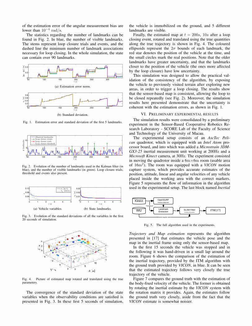
of the estimation error of the angular measurement bias arelower than 10−4 rad/s.

The statistics regarding the number of landmarks can befound in Fig. 2. In blue, the number of visible landmarks.The stems represent loop closure trials and events, and thedashed line the minimum number of landmark associationsnecessary for loop closing. In the whole simulation, the statecan contain over 90 landmarks.

50 100 150 200 250 3000

0.2

0.4

‖pi−pi‖[m

]

t [s]

(a) Estimation error norm.

50 100 150 200 250 3000

0.2

0.4

0.6

0.8

σpi[m

]

t [s]

(b) Standard deviation.

Fig. 1. Estimation error and standard deviation of the first 5 landmarks.

50 100 150 200 250 3000

5

10

#landmarks

t [s]

Observed landmarksLoop closure eventsLoop closure trialsLoop closure threshold

Fig. 2. Evolution of the number of landmarks used in the Kalman filter (inblue), and the number of visible landmarks (in green). Loop closure trials,threshold and events also present.

0 1 2 3 4 5

0.04

0.08

0.12

σ

t [s]

σv [m/s]σbω

[rad/s]

(a) Vehicle variables.

0 1 2 3 4 50

0.01

0.02

0.03

σpi[m

]

t [s]

(b) State landmarks.

Fig. 3. Evolution of the standard deviations of all the variables in the first20 seconds of simulation.

Fig. 4. Picture of estimated map rotated and translated using the trueparameters.

The convergence of the standard deviation of the statevariables when the observability conditions are satisfied ispresented in Fig. 3. In these first 5 seconds of simulation,

the vehicle is immobilized on the ground, and 5 differentlandmarks are visible.

Finally, the estimated map at t = 200s, 10s after a loopclosing event, rotated and translated using the true quantitiesalong the true trajectory is shown in Fig. 4. The colouredellipsoids represent the 2σ bounds of each landmark, thered star denotes the position of the vehicle at the time, andthe small circles mark the real positions. Note that the olderlandmarks have greater uncertainty, and that the landmarkscloser to the position of the vehicle (the ones more affectedby the loop closure) have low uncertainty.

This simulation was designed to allow the practical val-idation of the consistency of the algorithm, by exposingthe vehicle to previously visited terrain after exploring newareas, in order to trigger a loop closing. The results showthat the sensor-based map is consistent, allowing the loop tobe closed repeatedly (see Fig. 2). Moreover, the simulationresults here presented demonstrate that the uncertainty iscoherent with the estimation errors, as shown in Fig. 1.

VI. PRELIMINARY EXPERIMENTAL RESULTS

The simulation results were consolidated by a preliminaryexperiment in the Sensor-Based Cooperative Robotics Re-search Laboratory - SCORE Lab of the Faculty of Scienceand Technology of the University of Macau.

The experimental setup consists of an AscTec Peli-can quadrotor, which is equipped with an Intel Atom pro-cessor board, and into which was added a Microstrain 3DM-GX3-25 inertial measurement unit working at 200Hz and aMicrosoft Kinect camera, at 30Hz. The experiment consistedin moving the quadrotor inside a 6m×6m room (usable areaof 16m2). The room was equipped with a VICON motioncapture system, which provides accurate estimates of theposition, attitude, linear and angular velocities of any vehicleplaced inside the working area with the correct markers.Figure 5 represents the flow of information in the algorithmused in the experimental setup. The last block named Inertial

[17]

Fig. 5. The full algorithm used in the experiments.

Trajectory and Map estimation represents the algorithmpresented in [17] that estimates the vehicle pose and themap in the inertial frame using only the sensor-based map.

In the first 15 seconds the vehicle was stopped and inthe following it was hand-driven in a small lap around theroom. Figure 6 shows the comparison of the estimation ofthe inertial trajectory, provided by the ITM algorithm withthe ground truth provided by VICON, in blue. It can be seenthat the estimated trajectory follows very closely the truetrajectory of the vehicle.

Figure 7 compares the ground truth with the estimation ofthe body-fixed velocity of the vehicle. The former is obtainedby rotating the inertial estimate by the VICON system withthe rotation matrix it provides. Again, the estimates followthe ground truth very closely, aside from the fact that theVICON estimate is somewhat noisier.

0 5 10 15 20 25 30 35

−2

0

2

x[m

]

t [s]

SLAMVICON

0 5 10 15 20 25 30 35

−2

0

2

y[m

]

t [s]

SLAMVICON

0 5 10 15 20 25 30 35

−2

0

2

z[m

]

t [s]

SLAMVICON

Fig. 6. Time evolution of the real and estimated trajectory

0 5 10 15 20 25 30 35

−0.5

0

0.5

u[m

]

t [s]

SLAM95% boundsVICON

0 5 10 15 20 25 30 35

−0.5

0

0.5

v[m

]

t [s]

SLAM95% boundsVICON

0 5 10 15 20 25 30 35

−0.2

0

0.2

w[m

]

t [s]

SLAM95% boundsVICON

Fig. 7. Time evolution of the real and estimated velocity

0 5 10 15 20 25 30 350

20

40

#landmarks

t [s]

Stored landmarksObserved landmarks

Fig. 8. Evolution of the number of landmarks used in the Kalman filter(in blue) and the visible (in green).

Finally, the evolution of the number of landmarks involvedin the algorithm are shown in Fig. 8. In blue, the number oflandmarks in the SLAM filter state are presented. Note theconstant number while the vehicle is stopped. The numberof visible landmarks in each instant is shown in green. Notethat just after the first 30 s the number of observation instantsis small (due to technical problems with the equipment) andthe number of visible landmarks is also very small, whichexplains the degradation in the estimation that occurs aroundthat time.

VII. CONCLUSIONS AND FUTURE WORK

This paper presented the design, analysis, simulation,and preliminary experimental validation of a novel glob-ally asymptotically stable sensor-based SLAM filter. Theframework in which all work is based is intended to filterwithin the space of the sensors, thus avoiding the attituderepresentation in the filter state. The main focus of this workwas the observability analysis, which provided theoreticalresults in observability and, subsequently, on the convergenceof the error dynamics of the proposed nonlinear system.

Furthermore, the performance and consistency of the algo-rithm were validated in simulation showing the convergenceof the uncertainty in every variable except the non-visiblelandmarks, as well as the production of a consistent mapwhich allows the closure of a loop with nearly 50 meters.Preliminary experimental results, with ground truth data,showed also the good performance of the SLAM filter andhinted at the good estimation of the transformation to theinertial frame.

The complete algorithm involves two different mainblocks, the SLAM filter on one side, and an Inertial Tra-jectory and Map Estimation algorithm on the other, usingas inputs the sensor-based estimated map [17]. Future workmay also address the inclusion of landmark directions andthe establishment of necessary conditions in the observabilityanalysis.

REFERENCES

[1] G. N. DeSouza and A. C. Kak, “Vision for Mobile Robot Navigation:A Survey,” IEEE Transactions on Pattern Analysis and MachineIntelligence, vol. 24, no. 2, pp. 237–267, 2002.

[2] H. Durrant-Whyte and T. Bailey, “Simultaneous Localisation andMapping (SLAM): Part I The Essential Algorithms,” IEEE Robotics& Automation Magazine, vol. 13, no. 2, pp. 99–110, 2006.

[3] T. Bailey and H. Durrant-Whyte, “Simultaneous localization andmapping (SLAM): Part II,” IEEE Robotics & Automation Magazine,vol. 13, no. 3, pp. 108–117, 2006.

[4] J. Castellanos, R. Martinez-Cantin, J. Tardos, and J. Neira, “Robocen-tric map joining: Improving the consistency of EKF-SLAM,” Roboticsand Autonomous Systems, vol. 55, no. 1, pp. 21 – 29, 2007.

[5] S. Huang and G. Dissanayake, “Convergence and Consistency Analy-sis for Extended Kalman Filter Based SLAM,” IEEE Transactions onRobotics, vol. 23, no. 5, pp. 1036 –1049, October 2007.

[6] S. Julier and J. Uhlmann, “A counter example to the theory ofsimultaneous localization and map building,” in Proc. of the 2001IEEE Int. Conf. on Robotics and Automation (ICRA), vol. 4, Seul,South Korea, May 2001, pp. 4238–4243.

[7] S. Se, D. Lowe, and J. Little, “Mobile Robot Localization andMapping with Uncertainty using Scale-invariant Visual Landmarks,”The International Journal of Robotics Research, vol. 21, no. 8, pp.735–758, 2002.

[8] F. Endres, J. Hess, N. Engelhard, J. Sturm, D. Cremers, and W. Bur-gard, “An Evaluation of the RGB-D SLAM System,” in Proc. of theIEEE Int. Conf. on Robotics and Automation (ICRA), St. Paul, MA,USA, May 2012.

[9] B. Guerreiro, P. Batista, C. Silvestre, and P. Oliveira, “Sensor-basedSimultaneous Localization and Mapping - Part I: GAS RobocentricFilter,” in Proc. of the 2012 American Control Conference, Montreal,Canada, Jun. 2012, pp. 6352–6357.

[10] ——, “Sensor-based Simultaneous Localization and Mapping - PartII: Online Inertial Map and Trajectory Estimation,” in Proc. of the2012 American Control Conference, Montreal, Canada, Jun. 2012, pp.6334–6339.

[11] P. Batista, C. Silvestre, and P. Oliveira, “Single range aided navigationand source localization: Observability and filter design,” Systems &Control Letters, vol. 60, no. 8, pp. 665 – 673, 2011.

[12] R. Brockett, Finite Dimensional Linear Systems, ser. Series in decisionand control. John Wiley & Sons, 1970.

[13] B. Anderson, “Stability properties of Kalman-Bucy filters,” Journal ofthe Franklin Institute, vol. 291, no. 2, pp. 137 – 144, 1971.

[14] P. Batista, C. Silvestre, and P. Oliveira, “Sensor-based ComplementaryGlobally Asymptotically Stable Filters for Attitude Estimation,” inProc. of the 48th IEEE Conference on Decision and Control, Shanghai,China, 2009, pp. 7563–7568.

[15] H. Bay, A. Ess, T. Tuytelaars, and L. V. Gool, “Speeded-Up RobustFeatures (SURF),” Computer Vision and Image Understanding, vol.110, no. 3, pp. 346 – 359, 2008, Similarity Matching in ComputerVision and Multimedia.

[16] J. Neira and J. Tardos, “Data Association in Stochastic Mapping Usingthe Joint Compatibility Test,” IEEE Transactions on Robotics andAutomation, vol. 17, no. 6, pp. 890 –897, dec 2001.

[17] P. Lourenco, B. J. Guerreiro, P. Batista, P. Oliveira, and C. Silvestre,“3-D Inertial Trajectory and Map Online Estimation: Building on aGAS Sensor-based SLAM filter,” in European Control Conference2013, July 2013, accepted.