arX

iv:g

r-qc

/000

6108

v1 3

0 Ju

n 20

00

Assisted inflation in

Friedmann-Robertson-Walker and Bianchi

spacetimes

Juan M. Aguirregabiria, Alberto Chamorro,

Fısica Teorica, Universidad del Paıs Vasco,

Apdo. 644, 48080 Bilbao, Spain,

Luis P. Chimento and Norberto A. ZuccalaDepartamento de Fısica,

Facultad de Ciencias Exactas y Naturales,

Universidad de Buenos Aires

Ciudad Universitaria, Pabellon I,

1428 Buenos Aires, Argentina.

February 7, 2008

Abstract

We use exact general solutions for the spatially flat FRW and

the anisotropic Bianchi I cosmologies to show that generically un-

coupled scalar fields cooperate to make inflation more probable, while

the presence of several interacting fields hinders the occurrence of the

phenomenon, in accordance with previous results based on particular

power-law solutions. Similar conclusions are reached in the case of

Bianchi VI0 spacetimes, for power-law solutions which are proved to

be attractors.

PACS 04.20.Jb

1

1 Introduction

In many inflationary models the effective potential energy density of a scalarfield is responsible for an epoch of accelerated inflationary expansion [1]. Veryoften one assumes that inflation is driven by a scalar field of the Liouvilleform, i.e., a exponential potential, because this kind of potential arises invarious higher-dimensional supergravity [2] and superstring [3] models [4, 5,6, 7].

Although there are many scalar fields in superstring theories, in the pastit was often assumed that typically only one scalar field was responsible forthe inflation, while those having higher exponents were quickly redshiftedaway. However, it has been found [8] that the so-called assisted inflation

may occur when several scalar fields are present, even if each individual fieldis too steep to drive the inflation, provided that the fields are uncoupled andinteract only through the geometry. On the other hand, if the fields interactdirectly with each other, the opposite effect may happen and the presence ofcross couplings beteween fields may hinder inflation [9, 10, 11].

Assisted inflation has been mainly studied in power-law solutions (a ∝ tp)for the spatially flat Friedmann-Robertson-Walker (FRW) cosmology, whichcan be shown [8] to be the late-time attractor for the evolution of this kind ofmodel. (Recently, Green and Lidsey [12] discussed in the context of assistedinflation the late-time evolution in a general geometry.)

The purpose of this work is to extend previous studies on multi-scalarfield cosmologies in two directions: firstly, we will use general solutions (in-stead of the special power-law ones) to analyze if the presence of severalfields generically helps or impedes inflation, and secondly, going beyond theaforementioned FRW cosmology, we will consider the anisotropic inhomoge-neous generalization given by Bianchi type I models. Thus in section 2.1 wedeal with n interacting scalar fields in a FRW spacetime and use the generalsolution to show that the larger is the number of interacting scalar fields theless likely is inflation. Section 2.2 makes plausible for more general scalarfield potentials the results obtained in section 2.1 for exponential potentials.We do not know the solution for n non-interacting scalar fields in a FRWcosmology in the general case, but we use the discussion of the late-time at-tractor of section 2.3 to restrict the analysis of uncoupled fields in section 2.4to the particular case in which all fields are assumed to be equal, for whichthe general solution can be found. We show that non-interacting fields gener-ically cooperate to assist inflation. The density fluctuations correspondingto the last case are discussed in section 2.5. General solutions of anisotropicBianchi I cosmologies with interacting and uncoupled fields are used in thefirst part of section 3.1 and subsection 3.2, respectively, to check that also in

2

those cases interacting fields make inflation more difficult while uncoupledfields assit it. The stability of power-law solutions is dicussed in 3.3. Fi-nally in section 4 we turn to power-law solutions of the Bianchi VI0 model,reaching again the same conclusions.

2 The n-scalar field problem in a flat FRW

spacetime

In the following we will consider two kinds of problems in flat FRW space-times in which there are n homogeneous scalar fields driven by exponentialpotentials. First of all, we will assume that the scalar fields are interactingthrough a product of exponential potentials. Then we will consider the casein which the scalar fields are uncoupled because the potential is a sum ofpotentials involving a single field.

2.1 The interacting n-scalar field problem in flat FRW

spacetime

The problem of n interacting homogeneous scalar fields, φi, driven by a prod-uct of n exponential potentials Vi = V0ie

−kiφi minimally coupled to gravityin a flat Robertson-Walker spacetime, with metric

ds2 = −dt2 + a2(t)[

dx2 + dy2 + dz2]

, (1)

is formulated by the system of equations

3H2 =1

2φ2 + V, (2)

~φ+ 3H~φ− V ~k = 0, (3)

where H = a/a and the potential

V (~φ) = V0e−~k·~φ, (4)

allows for interactions between the fields. V0 is the constant V01V02 · · ·V0n,and ~k = (k1, k2, ..., kn) is an n -component constant vector with respect to anorthonormal basis in the n -dimensional Euclidean internal space to whichthe vector ~φ = (φ1, φ2, ..., φn), built with the n minimally coupled scalarfields, also belongs. In the remaining of this section k, k2 and φ2 stand

for∣

∣

∣

~k∣

∣

∣, ~k · ~k, and ~φ · ~φ respectively. Potentials of this type are of interest

3

because they may be considered just as an approximation to a more complexpotential. In fact, in higher-dimensional superstring theories, the scalar fieldis like one of the matter fields that contribute to the action and effectivepotential of the theory. Loop expansion [3], or expansion in the number ofinteracting particles [13], of the action leads to a perturbative expression ofthe potential which is a summation of exponential terms [5, 6]. From (2)–(3),and discarding the trivial static metric solution H = 0, 1

2φ2 + V = 0 , we get

H = −1

2φ2. (5)

Using this equation and the system (2)–(3) one finds that the Klein-Gordonequations (3) have the first integrals

~φ = H~k +~c

a3, (6)

where ~c = (c1, c2, ..., cn) is an arbitrary vector integration constant. As (6)involves only geometrical quantities the Einstein-Klein-Gordon equations un-couple and the general parametric solution can be obtained [14], [15], [16].

One can easily verify that in this kind of models the Einstein-Klein-Gordon equations have power-law solutions

a ∝ t2

k2 , (7)

so that they inflate at all times when k2 < 2. We will show below that thegeneral solution has the same kind of behavior when the scale factor a islarge enough.

Inserting (6) in (5) we obtain the following second-order equation for thescale factor a(t)

s+ sms+1

4 cos2 σs2m+1 = 0, (σ 6= π/2), (8)

where

cosσ =~c · ~kck

, (9)

m = −6/k2 < 0, c = |~c|, a and t have been replaced by the new variables sand τ defined by

a = s−m3 , τ = ckt cosσ, (10)

and the dot stands for derivation with respect to τ . Once s(τ) is known one

can compute, in principle, the scale factor a(τ) from (10 ), and the fields ~φ(t)from equations (6).

4

Equation (8) is a particular case of the second order nonlinear ordinarydifferential equation

s+ αf(s)s+ βf(s)∫

f(s) ds+ γf(s) = 0, (11)

where f(s) is some real function and α, β and γ are constant parameters.Depending on the values of k2 our equation (8) corresponds to the next twocases:

1. k2 6= 6 and

f(s) = sm, α = 1, β =m+ 1

4 cos2 σ, γ = 0. (12)

2. k2 = 6 and

f(s) =1

s, α = 1, β = 0, γ =

1

4 cos2 σ. (13)

Inserting the first integrals (6) in the Einstein equation (2 ), we get aquadratic equation in the expansion rate H which has real solutions onlywhen its discriminant is non-negative. This condition leads to

β ≤ 1

4[

1 + 2a6Vc2

] <1

4, (14)

discarding the oscillatory solutions of equation (11), which would be obtainedfor a negative potential or β > 1/4. It follows that, if k2 6= 6, real solutionsexist always for

k2 < k20 =

6

sin2 σ. (15)

This sets a restriction on the integration constants and the exponent of theexponential-potential.

The general solution of (11) can be obtained making the nonlocal trans-formation of variables [17]

z =∫

f(s) ds, η =∫

f(s) dτ. (16)

Under this transformation (8) becomes a linear inhomogeneous ordinary dif-ferential equation with constant coefficients

z′′ + αz′ + βz + γ = 0, (17)

5

which for α > 0 and β > 0 is the equation of a damped harmonic oscillatorin a constant external field. Here the ′ indicates differentiation with respectto η. In our case the nonlocal transformation of variables (16) is

z =sm+1

m+ 1, η =

∫

sm dτ , (18)

for k2 6= 6, and

z = ln s, η =∫ dτ

s, (19)

for k2 = 6.Taking α = 1 in (17) we get

z =

b1eλ+η + b2e

λ−η, for k2 6= 6;

b1 + b2e−η − γη, for k2 = 6;

(20)

where

λ± =−1 ±

√1 − 4β

2, (21)

and b1, b2 are real integration constants.We see from (10) and (18) that

a ∝ z−m

3(m+1) , (22)

so that, while for k2 > 6 the scale factor goes to 0 as z → 0, one has thatfor k2 < 6 the scale factor goes to infinity when z → 0. On account ofequations (20) one may assume that the latter occurs as η → η0, for anappropriate value of η0. Let us now write η = η0 + δη and expand (20)and (22) about z = 0 and η = η0, keeping only terms linear in δη, so thatδz = δη and

a = δz−m

3(m+1) = δη−m

3(m+1) . (23)

Now, we see from (10) and (18) that

δη = a−3δτ ∝ a−3δt. (24)

If we use this in (23), we get successively

a ∝ am

m+1 δt− m

3(m+1) , (25)

anda ∝ δt−

m3 = δt

2k2 . (26)

We see then that if k2 < 2 the solution does inflate at least along some timeinterval. Now, since k2 = k2

1 + k22 + · · ·+ k2

n, one concludes from our analysis

6

of the general solution that the larger is the number of the interacting scalarfields the less likely will be k2 < 2 as well that inflation take place. On theother hand, for 6 < k2 < k2

0, one has 0 < β < 1/4 that implies that bothλ± < 0; thus (18) and ( 20) tell us that the scale factor goes to infinitywhen z → ∞ and η → −∞ (with no loss of generality we are taking bothconstants b1, b2 > 0). By keeping only the dominant terms we have for verylarge negative η that

a ∝ e−mλ

−η

3(m+1) . (27)

This relation and (24), that is generally valid, yield

δa

a∝ a−3δt (28)

whose general solution is a ∝ t1/3. In this case the solution does not in-flate and it approaches to the free scalar field solution. These results arein accordance with those obtained with particular solutions by other au-thors [9, 10, 11].

It would be surprising if for k2 = 6 the scale factor had a behaviordrastically departing from that suggested by the previous analysis whenk2 ∈ (k2

0, 6)⋃

(6, 2). In fact, we see from (10) and (19) that z = 3 log aso that, as a consequence of (20), a goes to infinity as η → −∞. From (20)we see that log z ∼ −η, when η → −∞ and, by using (24),

δa

a log a∝ δz

z∼ −δη ∝ δt

a3, (29)

which can be written asδa

a∼ a−3δt log a. (30)

In the asymptotic regime in which a→ ∞ we have a δa < a2 δa/ log a < a2 δa,so that from (30) we get a2 <∼ t <∼ a

3 and, finally,

t1/3 <∼ a <∼ t1/2, when a→ ∞. (31)

We see that the solution does not inflate.

2.2 More general potentials

The results of the above section show that we can introduce an n -dimensionalEuclidean internal vector space containing the n-component vector ~φ =(φ1, φ2, ..., φn) built with n minimally coupled scalar fields. Let us assumenow that the potential has the general form

V = V (Φ), Φ = ~k · ~φ. (32)

7

In this case the Einstein equation (2) remains unchanged, however the Klein-Gordon equation (3) becomes

~φ+ 3H~φ+ V ′~k = 0. (33)

where the ′ indicates derivatives with respect to the variable Φ. Since (2), (32)and (33) are invariant under rotations of the orthogonal axes in the Euclideanspace above mentioned, we may choose the first axis of this internal spacealong the vector ~k. Then the Klein-Gordon equation splits into one equationfor φ1 = φ

φ+ 3Hφ+ kV ′ = 0, (34)

and n− 1 free field Klein-Gordon equations for φ2 = · · · = φn = ψ

ψ + 3Hψ = 0. (35)

From (35) we obtain the first integral ψ = c0/a3, where c0 is an arbitrary

integration constant. Hence the original n-scalar field problem is equivalentto considering a self-interacting scalar field with stiff matter. In fact, theEinstein equation (2) now reads

3H2 =1

2φ2 + V +

c2ψ2a6

, (36)

where c2ψ is the sum of n− 1 positive defined integration constants.Taking into account that the scalar field φ depends only on t, its energy-

momentum tensor may be written in the perfect fluid form

Tik = (pφ + ρφ)uiuk + pφgik , (37)

where

ρφ =1

2φ2 + V (φ) ,

pφ =1

2φ2 − V (φ). (38)

The fluid interpretation of the scalar field has proven very useful in the studyof the inflationary and Q-matter scenarios [18]. In particular it leads toconsider its equation of state pφ = (γφ − 1) ρφ. On the other hand, the stateequation for fluid representing stiff matter is pf = (γf − 1) ρf with γf = 2.Because of the additivity of the stress-energy tensor it makes sense to consideran effective perfect fluid description with equation of state p = (γ − 1) ρwhere p = pf + pφ, ρ = ρf + ρφ and

γ =γfρf + γφρφρf + ρφ

(39)

8

is the overall (i.e. effective) adiabatic index. For this effective perfect fluidthe dynamical equations are

3a2

a2= ρ (40)

anda

a= −1

6[ρ+ 3p] , (41)

where p and ρ are the density and pressure of the effective perfect fluid.They involve the self-interacting scalar field and the n-1 free scalar fields.Inflationary solutions occur when a > 0; this means that the expansion isdominated by a gravitationally repulsive stress that violates the strong energycondition ρ+3p < 0 or equivalently γ < 2/3 . When we impose this conditionon (39), we obtain that

V (Φ) > φ2 +c2ψa6. (42)

Hence, when there is only one scalar field the solution inflates for V (φ) >φ2. However, the n interacting scalar fields produce a desassisted inflationbecause the solutions inflate only if (42) holds. Using the effective perfectfluid description we can generalize this analysis to an arbitrary potentialV (φ1, φ2, ..., φn). In this case we obtain that V (φ1, φ2, ..., φn) > φ2

1 + φ22 +

..... + φ2n, so that the interacting n scalar fields might make inflation more

unlikely in a FRW spacetime.

2.3 The n-scalar field attractor problem in the FRW

spacetime

Let us now assume that the n homogeneous scalar fields, φi, in the FRWspacetime are driven by a general potential V = V (φi). In that case theEinstein-Klein-Gordon equations are

3H2 =1

2

n∑

i=1

φ2i + V, (43)

φi + 3Hφi + V,φi= 0. (44)

where V,φistand for ∂V/∂φi. From these equations we get

H = −1

2

n∑

i=1

φi2. (45)

9

In order to investigate the stable scalar field configurations, we introducethe quantity

ω =

∑ni=1 φi

2

nφ2α

, (46)

which reduces to ω = 1 for the configuration φ1 = φ2 = · · · = φn. Using(43)–(46) we find the differential equation for ω:

ω = 2nV,φα

φαω − V

nφ2α

. (47)

(In this section no summation convention applies to repeated Greek indexes.)If we further assume that the potential satisfies the condition

V = nV,φαφα, (48)

equation (47) becomes

ω = 2V,φα

φα(ω − 1) (49)

which has a fixed point solution: ω = 1. Furthermore, the general solutionof (49) can be found using (44):

ω = 1 +c

a6φ2α

(50)

where c is an arbitrary integration constant. However, it is useful to expressthe last solution in terms of geometrical quantities with the aid of (45) and(46). The final result is

ω =(

1 +nc

2a6H

)−1

. (51)

Evaluating (51) in the asymptotic regime, it can be easily shown that theparticular solution ω = 1 is an attractor for evolutions that behave asymp-totically as a ∝ tν with ν > 1/3.

This result strongly suggests that the special case in which all scalarfields are equal may be the late-time attractor of more general problems. Infact, this has been proved in [9] for potential (4) with k1 = · · · = kn andV01 = · · · = V0n, which guarantee assumption (48). We did not use this factin the previous section because we were able to use the general solution withno additional assumption on ki, V0i and φi, but it will be useful to simplifysomewhat the problem analyzed in the following section.

10

2.4 The non-interacting n-scalar field problem in the

FRW spacetime

Let us now assume that the n homogeneous scalar fields, φi, in the spacetimegiven by (1) do not interact directly, but are driven by a sum of n exponentialpotentials Vi = V0ie

−kiφi. In that case the Einstein-Klein-Gordon equationsare

3H2 =n∑

i=1

[

1

2φ2i + Vi

]

, (52)

φi + 3Hφi − kiVi = 0. (53)

From now on we will consider a simplified problem in which k1 = k2 =· · · = kn ≡ k and V01 = V02 = · · · = V0n ≡ V0. As discussed in the previoussection, we can expect in this particular case that in the asymptotic evolutionall scalar fields tend to a common limit. That this is actually the case hasbeen proved in [8]. In consequence, in the remaining of this section we willtake φ1 = φ2 = · · · = φn ≡ φ, so that V1 = V2 = · · · = Vn ≡ V = V0e

−kφ andequations (52)–(53) reduce to

3H2 =n

2φ2 + nV, (54)

φ+ 3Hφ− kV = 0. (55)

One can easily get from (54)–(55)

H = −n2φ2 (56)

and the first integral of the Klein-Gordon equation (55)

φ =k

nH +

c

a3, (57)

where c is an arbitrary integration constant.As in the previous section, the Einstein-Klein-Gordon equations have

power-law solutions [8]

a ∝ t2n

k2 , (58)

so that this type of solutions inflates at all times when k2 < 2n. We willnow show that the general solution of the Einstein-Klein-Gordon equations( 54) and (55) has the same kind of behavior when the scale factor a is largeenough.

11

Inserting (57) in (56) we obtain the following second-order equation forthe scale factor a(t)

s + sms+1

4s2m+1 = 0, (59)

where m = −6n/k2 < 0, the dot means derivative with respect to τ and wehave used, instead of a and t, the new variables s and τ defined by

a = s−m3 , τ = ckt. (60)

We have again a particular case of equation (11) with α = 1 and tofind the general exact solution of (59) one has to consider the following twopossibilities:

1. k2 6= 6n and

f(s) = sm, β =m+ 1

4, γ = 0. (61)

2. k2 = 6n and

f(s) =1

s, β = 0, γ =

1

4. (62)

The general solution of (59) can be obtained by performing the nonlocaltransformation of variables given in (18)–(19) with the new value of m, whichreduces (59) to the linear inhomogeneous ordinary differential equation withconstant coefficients (17).

If one now repeats the analysis of the previous section by systematicallytaking σ = 0 and using the new m, the same final results for z and a areobtained: just replace k2 = k2

1 + · · · k2n by k2/n in the quantities involved

in (20) and (22). One readily concludes that, when a → ∞, these modelsinflate if k2 < 2n, so that the fields cooperate to make inflation more likelyin the so-called “assisted inflation”, which was first discussed —but only forpower-law solutions— in [8].

This result could have been anticipated since the present case is includedin the mathematical problem set in section 2.1 by equations (8) and (9) byjust taking cos σ = ±1 (that corresponds to the simplified problem underconsideration) and m = −6n/k2.

2.5 Density fluctuations

The fact that the contributions of the density fluctuations differ significantlyin different inflationary universe models, has motivated a detailed study ofall the alternatives. In this context, it is interesting to derive the spectral

12

indices for the perturbations that would be created during the periods ofinflation described by the solutions given in the last section. It is well knownthat, for multi-scalar field models, the spectrum of the curvature perturbationreads [19],

PS =(

H

2π

)2 ∂N

∂φi

∂N

∂φjδij , (63)

where N is the number of e-foldings of inflationary expansion remaining,and there is a summation over i and j. In the case considered in the previoussection,where all the scalar fields are equal, (63) yields [8]

PS(k) =(

H

2π

)2 1

n

H2

φ2

⌋

aH=k

. (64)

where H and φ have to be evaluated at the time when the wave number ofinterest k leaves the horizon during inflation. Also in this case, the spectralindex nS(k) defined as

nS(k) = 1 +d lnPS

d ln k

is given by [19, 8]

1 − nS = −2H

H2. (65)

The availability of exact solutions allows us to express the relevant quanti-ties as functions of the variable η introduced in equation (16). The scalefactor reads (see (22), which is satisfied for uncoupled scalar fields withm = −6n/k2, as one can easily see)

a(η) = [(m+ 1) z(η)]−m

3 (m+1) (66)

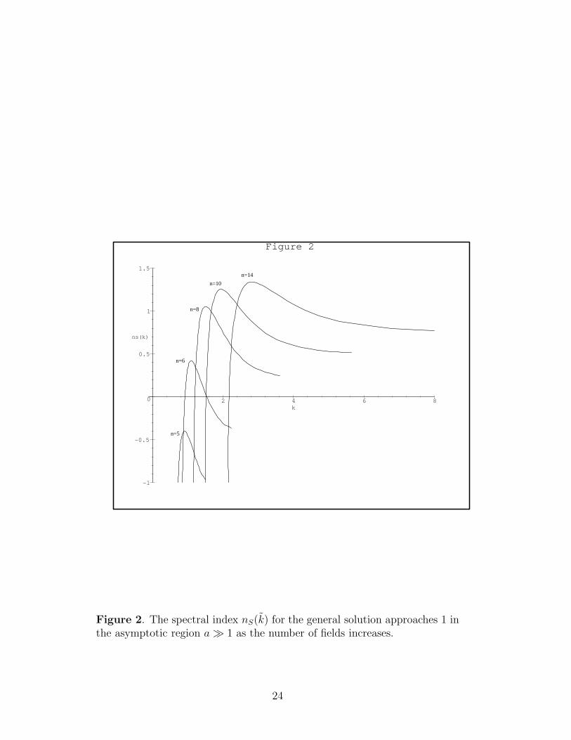
where z(η) is given by (20)–(21). The spectrum PS(k) obtained from (64)is shown in Figure 1, for k = 3, c = −1, b1 = −1, b2 = 0.001 and differentvalues of n. Here, inflation is possible for n ≥ 5, and one can see that thepeak of the spectral distribution moves towards the high frequency region asn increases. The corresponding spectral index nS is shown in Figure 2. From(65) and the general solutions (20), (21) and (66), it can be shown that thevalue of nS → 1 in the asymptotic region a ≫ 1 as the number n of presentfields increases. This feature is exemplified in Figure 2, where we can see howthe larger is the value of n, the closer is the spectrum to the scale invariance[8].

13

3 The n-scalar field problem in Bianchi type

I models

Now we turn to the general Bianchi type I model with n homogeneous scalarfields driven by exponential potentials. As we proceeded in the case of FRWspacetimes, we will first assume that the scalar fields are interacting througha product of exponential potentials, an then we will consider the case in whichthe scalar fields are uncoupled because the potential is a sum of potentialsinvolving a single field.

3.1 The interacting n-scalar field problem in the aniso-

tropic Bianchi type I model

The general Bianchi type I model is the anisotropic generalization of thespatially flat FRW universe expanding differently in the x, y, and z directions.In the usual synchronous form its line element is given by

ds2 = −dT 2 + a21(T ) dx2 + a2

2(T ) dy2 + a23(T ) dz2. (67)

For convenience we use the semiconformal coordinates

dt ≡ dT

a3, ef ≡ a2

3, G ≡ a1a2, ep ≡ a1

a2, (68)

to cast the metric (67) into the form

ds2 = ef(t)(

−dt2 + dz2)

+G(t)(

ep(t) dx2 + e−p(t) dy2)

. (69)

We first consider, as in section 2.1, n scalar fields φi interacting directlythrough the exponential potential (4). The problem of n interacting homo-geneous scalar fields, φi, driven by a product of n exponential potentialsVi = V0ie

−kiφi , minimally coupled to gravity in the Bianchi I spacetime (69),is formulated by the following system of Einstein-Klein-Gordon equations

p =a

G, (70)

ef =G

2V G, (71)

G

G− 1

2

(

G

G

)2

− G

Gf +

1

2p2 = −φ2, (72)

~φ+G

G~φ− ef V ~k = 0, (73)

14

where a is an arbitrary integration constant. It can be easily seen that thevector

~φ =G

G

~k

2+~m

G, (74)

(where ~m is a n-dimensional vector whose components are integration con-stants) is a first integral of the Klein-Gordon equation set (73). Inserting(70) in equation (74) the general solution of the Klein-Gordon equations isfound:

~φ = ~φ0 + p~m

a+~k

2lnG, (75)

where ~φ0 is an arbitrary constant vector. Equations (70 )–(72) along with(75) uncouple and their solutions can be obtained if one is able to solve thefollowing third-order equation for G

GG2 −...

GGG+

(

1

2− k2

4

)

GG2 +

(

m2 +a2

2

)

G = 0. (76)

Once G(t) is known, in principle one can compute p(t) and ~φ(t) from equa-tions (70) and (75), respectively; f(t) is then obtained from (71).

The Einstein-Klein-Gordon equations admit power-law solutions, G = tα,but they happen to be isotropic and, thus, equal to the ones discussed insection 2.1. Thus we will analyze, instead, the general solution of (76).

Equation (76) has the first integral

GG

G+ (K − 1)G+

M2

G= C, (77)

where C is an arbitrary constant and

K ≡ k2

4− 1

2, M2 ≡ m2 +

a2

2. (78)

If instead of t and G we use the new variables z and τ defined, for C 6= 0,in

G = z1/K , t = − τ

C, (79)

then, equation (77) becomes

z′′ + z−1/Kz′ +KM2

C2z1−2/K = 0, (80)

where a prime denotes the derivative with respect to τ . This equation is, oncemore, a particular case of (11) and can be linearized by using the non-localtransformation (16), which in this case is

y ≡∫

z−1/K dz = Kz1−1/K

K − 1, η ≡

∫

z−1/K dτ = −Cap (81)

15

for K 6= 1, and

y ≡∫

z−1 dz = ln z, η ≡∫

z−1 dτ = −Cap, (82)

for K = 1. If we take

β ≡ (K − 1)M2

C2, γ = 0, (83)

for K 6= 1 and

β = 0, γ =M2

C2, (84)

for K = 1, equation (80) reduces to two particular cases of equation (17) forα = 1. The trivial solution of this equation gives the implicit general solutionof (76) which can be written, for arbitrary a, M and non-vanishing C, as

G =[

e−η/2(

C1eλη + C2e

−λη)]

1K−1 (85)

for K 6= 1, and asG = C1e

−γη+C2e−η

(86)

for K = 1. C1 and C2 are integration constants and λ =√

1 − 4β/2.To check whether a model inflates, we will look at the sign of the decel-

eration parameter q = −θ−2(

3θ + θ2)

, where θ = ua;a is the expansion and

θ = θ,aua, ua being the four-velocity of the cosmic fluid. Since in this case

we are dealing with comoving coordinates, ua =(

e−f/2, 0, 0, 0)

, one can seethat, apart from a positive factor, the deceleration is

q ∝ 9KG2 − 3(2km+ C) + (km− C)2 + 9M. (87)

We see from (85) that when K < 1 (i.e., when k2 < 6) G blows upfor some value η = η0 = 1

2λlog (−C2/C1), provided that C1C2 < 0. If we

expand (85) around this value (η = η0 + δη) we get

G ∝ δη1

K−1 , (88)

and from (79) and (81)

dη =dτ

G= −C

Gdt, (89)

so that

G = −CGG′ ∝ 1

K − 1δη−1. (90)

16

In consequence, when G→ ∞ the deceleration parameter (87) is

q ∝ 9KC2

(K − 1)2

1

δη2, (when δη → 0), (91)

and there is inflation if K < 0, i.e., if k2 = k21 +k2

2 +· · ·+k2n < 2. We conclude

that in these anisotropic universes also a greater number of interacting scalarfields makes inflation less likely.

3.2 The non-interacting n-scalar field problem in the

Bianchi type I model

We will now assume that the n homogeneous scalar fields φi in the metric (67)do not interact directly, but are driven by a sum of n exponential potentialsVi = V0ie

−kiφi . To simplify the task of finding exact solutions of the Einstein-Klein-Gordon equations, we will further assume that k1 = k2 = · · · = kn ≡ k,φ1 = φ2 = · · · = φn ≡ φ and V1 = V2 = · · · = Vn ≡ V = V0e

−kφ, so thataforementioned equations can be written as

p =a

G, (92)

ef =G

2nV G, (93)

G

G− 1

2

(

G

G

)2

− G

Gf +

1

2p2 = −nφ2, (94)

φ+G

Gφ− kef V = 0, (95)

where a is an arbitrary integration constant. It is easy to check that

φ =k

2n

G

G+m

G(96)

is a first integral of the Klein-Gordon equation (95), in terms of the newintegration constant m. Inserting (92) in equation ( 96) the general solutionof the Klein-Gordon equations is found:

φ = φ0 + pm

a− k

2nlnG, (97)

where φ0 is an arbitrary constant. The equations (92)–( 94) along with(97) uncouple and their solutions can be obtained if one is able to solve thefollowing third-order equation for G

GG2 −...

GGG+

(

1

2− k2

4n

)

GG2 +

(

m2 +a2

2

)

G = 0. (98)

17

Since this equation is the same as (76) once one replaces k2 = k21 + k2

2 +· · · + k2

n by k2/n, we may repeat the calculations of the previous sectionto reach the opposite conclusion: if several non-interacting scalar fields arepresent, they will cooperate to “assist” the inflation, which will be more likelyand occurs for k2 < 2n.

3.3 Stability of power-law solutions in Bianchi type I

model

For many purposes it is interesting to investigate the stability of the solutionsof (76). In particular, we hope that the solution representing an acceleratedexpansion of the universe, and the solutions that correspond to the assistedinflation, be stable. To this end we introduce the variable

Ω =h

h2, (99)

where h = GG, in equation (76):

Ω +

[

Ω +K − M2

h2G2

]

(Ω + 1)h = 0. (100)

This equation has the fixed point solution Ω = −1. Note that equation (100)has also the fixed point solution Ω = −K if G → ∞ asymptotically. Thecorresponding asymptotic limits of these solutions can be obtained by solving(99) for them. The final result is G ∝ t and G ∝ t1/K respectively. Let usinvestigate the stability of these solutions when G blows up. From (100) it iseasy to see that Ω = −1 is unstable because expanding the solutions aboutit, Ω = −1 + ǫ with ǫ ≪ 1, the sign of ǫ depend on the slope of potentialand the initial conditions. In fact, the corresponding solution G ∝ t does notsatisfies Einstein equations (cf. (93)) and was introduced when multiplying(94) with G2G to obtain (98). On the other hand, the asymptotic solutionΩ = −K is stable because the dynamical equation for the perturbation ǫ

ǫ = −1 −K

Ktǫ (101)

near the attractor indicates that ǫ decreases for K < 1. In particular, theinflationary solutions, that occur for K < 0, are stable.

18

4 The n-scalar field problem in a Bianchi VI0

model

The Bianchi VI0 model can be written as follows:

ds2 = ef(t)(

−dt2 + dz2)

+G(t)(

ez dx2 + e−z dy2)

. (102)

We first consider, as in previous sections, n scalar fields φi interactingthrough the exponential potential (4). The corresponding Einstein-Klein-Gordon equations are

ef =G

2V G, (103)

G

G− 1

2

(

G

G

)2

− G

Gf +

1

2= −φ2, (104)

~φ+G

G~φ− ef V ~k = 0. (105)

As formerly, one can check that the vector

~φ =G

G

~k

2+~m

G, (106)

where ~m is a n-dimensional arbitrary constant vector, is a first integral ofthe Klein-Gordon equation set (105). By using this result and the value off one obtains from (103), we get

GG2 −...

GGG+

(

1

2− k2

4

)

GG2 +1

2GG2 +m2G = 0. (107)

The solutions of this equation are not known. However, investigating thestability of its fixed points, the asymptotic behavior of the general solutioncan be obtained in a simple way. In order to see whether assisted inflationworks in Bianchi type VI0 metrics it is sufficient to analyze the special casem2 = 0. In terms of the variable Ω defined by (99), equation (107) becomes

Ω +[

Ω +K − 1

2h2

]

(Ω + 1)h = 0. (108)

This equation has three fixed points: Ω1 = −1, Ω2 = −K if h → ∞asymptotically, and Ω3 = 0, which correspond to G ∝ t, G ∝ t1/K andG ∝ et/

√2K respectively. Now, we investigate the stability of these solutions

19

when G blows up. Expanding the solution about fixed points, that is, makingΩ = Ω1,2,3 + ǫ with ǫ≪ 1, we get

ǫ =1

2hǫ (109)

for Ω1, which shows it is unstable, as in the case discussed in the previ-ous section. On the other hand, one obtains equation (101) for the linearapproximation around Ω2, and

ǫ = −√

1

2Kǫ (110)

in the case of Ω3. We conclude that the asymptotic solution Ω2 is stable forK < 0, which means k2 < 2 (for this set of potential slopes we have inflation),and Ω3 is stable forK > 0. Note thatG ∝ t1/K is only an asymptotic solutionof (107), with m = 0; however, it acts as an attractor for all solutions thatare close to it.

In this special case in which m2 = 0, one can readily see that the thedeceleration parameter for the solutions G ∝ t1/K is (after recovering theimplicit absolute value around t)

q ∝ K

1 −K|t|−2−1/K , (111)

which is negative for −1/2 ≤ K < 0. Again, the more interacting scalar fieldsthe less likely is inflation, which ensues when k2 = k2

1 + k22 + · · · + k2

n < 2.If one assumes now that the scalar fields do not interact directly and one

sets all the fields equal, as in sections 2.4 and 3.2, it is easily seen that theattracting power-law solutions inflate when k2 < 2n, so that the scalar fieldscooperate to assist inflation.

5 Conclusions

We have studied the effects of the appearance of more than one scalar fieldboth in FRW spacetimes and in anisotropic Bianchi I cosmologies. Insteadof using the important but particular power-law solutions, we have takenadvantage of the general solution to analyze the generic behavior in FRW.In Bianchi I the power-law solutions are isotropic and, thus, very particular,so that the use of the general solution is even more illustrative. In all caseswe have found, in agreement with calculations made by other authors withpower-law solutions in FRW, that the existence of more than one scalar

20

field assists inflation provided that they are uncoupled and interact onlythrough expansion. Also, in this case, the spectrum of density perturbationsbecomes closer to scale invariance as the number of fields increases. If, on thecontrary, the fields interact directly with each other, inflation is less likelyto occur. The same behavior has been obtained in Bianchi VI0 universes,but (not having available the general solution) only for power-law solutions,which have been shown to be attractors when inflation arises. These resultsreinforce our belief that the presence of several uncoupled scalar fields in moregeneral cosmologies fosters inflation, but that, in contradistinction, mutuallyinteracting scalar fields tend to hinder the inflationary process.

Acknowledgments

This work was partially supported by the University of the Basque Countrythrough the Research Project UPV172.310-EB150/98 and the General Re-search Grant UPV172.310-G02/99, as well as by the University of BuenosAires under Project TX93. We thank the anonymous referee for his helpfulcomments.

References

[1] L.F. Abbot and S.Y. Pi, Inflationary Cosmology, World Scientific, Sin-gapore (1986).

[2] A. Salam and E. Sezgin, Phys. Lett. 147B, 47 (1984).

[3] E.S. Fradkin and A.A. Tseytlin, Phys. Lett. 158B, 316 (1985).

[4] B.A. Campell, A. Linde and K.A. Olive, Nucl. Phys. B355, 146 (1991).

[5] M. Ozer and M.O. Taha, Phys. Rev. D45, 997 (1992).

[6] R. Easther, Class. Quantum Grav. 10, 2203 (1993).

[7] R. Easther, K. Maeda and D. Wands, Phys. Rev. D53, 4247 (1996).

[8] A.R. Liddle, A. Mazumdar and F.E. Schunck, Phys. Rev. D 58, 061301(1998).

[9] P. Kanti and K.A. Olive, Phys. Rev. D 60, 043502 (1999).

[10] S.W. Hawking and H.S. Reall, Phys. Rev. D 59, 023502 (1999).

21

[11] E.J. Copeland, A. Mazumdar and N.J. Nunes, astro-ph/9904309.

[12] A.M. Green and J.E. Lidsey, astro-ph/9907223.

[13] D.J. Gross and J.H. Sloan, Nucl. Phys. B291, 41 (1987).

[14] J.M. Aguirregabiria and L.P. Chimento, Class. Quantum Grav. 13, 3197(1996).

[15] L.P. Chimento, A.E. Cossarini N.A. and Zuccala, Class. Quantum Grav.15, 57 (1998).

[16] L.P. Chimento, Class. Quantum Grav. 15, 965 (1998).

[17] L.P. Chimento, J. Math. Phys. 38, 2565 (1997).

[18] L.P. Chimento, A.S. Jakubi and D. Pavon, Phys. Rev. D, 60 103501(1999).

[19] M. Sasaki and E.D. Stewart, Prog. Theor. Phys. 95, 71 (1996).

22

Figures

n=5 n=6 n=8 n=10

PS(k)

n=14

0

5

10

15

20

25

30

1 2 3 4 5 6k

Figure 1

Figure 1. Spectrum of the curvature perturbations for k = 3, c = −1,b1 = −1 and b2 = 0.001. As n increases (inflation is possible when n ≥ 5)the spectral distribution peak is shifted to high frequencies.

23

n=14

ns(k)

n=5

n=6

n=8

n=10

-1

-0.5

0

0.5

1

1.5

2 4 6 8k

Figure 2

Figure 2. The spectral index nS(k) for the general solution approaches 1 inthe asymptotic region a≫ 1 as the number of fields increases.

24