A Boundary Integral—Normal Mode Method
290
Scattering of Elastic Waves in Layered Media: A Boundary Integral—Normal Mode Method by Ronald T. Kessel B.A.Sc., University of Waterloo, 1984 M.Sc., University of Waterloo, 1989 A Dissertation Submitted in Partial Fulfillment of the Requirements for the Degree of Doctor of Philosophy in the Department of Physics We accept this dissertation as conforming to the required standard Dr. Trevor.W. Dawson, Supervisor (Adjunct Professor, Dept, of Physics and Astronomy) Dr. John. Weaver, Supervisor (Dean of Science, Dept, of Physics and Astronomy) Dr. Robert W. Stewart, Departmental Member (Adjunct Professor, Dept, of Physics and Astronomy) Dr. Pauline Van Den Driessche, Outside-Menjfej^fDepartment of Mathematics) Dr. Henrik Schmidt^ External Examiner '(DefjMJf Ocean Engineering, Massachusetts Institute of Technology) © Ronald T. Kessel, 1996 University of Victoria All rights reserved. This dissertation may not be reproduced in whole or in part, by photocopying or other means without the permission of the author.
-
Upload
khangminh22 -
Category
Documents
-
view
0 -
download
0
Transcript of A Boundary Integral—Normal Mode Method
Scattering of Elastic Waves in Layered Media: A Boundary Integral—Normal Mode Method
by
Ronald T. Kessel B .A .Sc., U niversity o f W aterloo, 1984
M .Sc., U niversity o f W aterloo, 1989
A Dissertation Submitted in Partial Fulfillment o f the Requirements for the Degree of
Doctor of Philosophy
in the Departm ent o f Physics
W e accept this dissertation as conform ing to the required standard
D r. Trevor.W . D aw son, Supervisor (A djunct Professor, Dept, o f Physics and A stronom y)
Dr. John. Weaver, Supervisor (Dean of Science, Dept, of Physics and Astronomy)
Dr. Robert W. Stewart, Departmental Member (Adjunct Professor, Dept, of Physics and Astronomy)
Dr. Pauline Van Den Driessche, Outside-Menjfej^fDepartment of Mathematics)
Dr. Henrik Schmidt^ External Examiner '(DefjMJf Ocean Engineering, Massachusetts Institute o f Technology)
© Ronald T. Kessel, 1996 University of V ictoria
All rights reserved. This dissertation may not be reproduced in whole or in part, by photocopying or other means without the permission of the author.
ii
Supervisor: Dr. Trevor W. DawsonAbstract
Elastic waves are used in geoacoustics to identify remote objects and events. Computer
models for such applications are being pressed to handle propagation in three dimensions,
and scattering from penetrable objects of arbitrary shape. One approach approximates earth
and ocean as horizontally stratified media into which the features of interest are embedded.
Here the Boundary Integral Equation (BIE) method for harmonic elastic wave scattering is
applied to layered media with penetrable fluid or solid inclusions. A new indirect method is
used to evaluate singular and poorly convergent BIE coefficients, the num erically
troublesome coefficients being inferred from free-field solutions o f the integral equation in
the absence of scattering. The new model is very flexible. M ultiple inclusions that are
penetrable or impenetrable, passive or actively vibrating, are permitted. Inclusions may have
edges, and may pass through interfaces between layers. A combined equation method is used
to over-determ ine the solution in the event of numerical instability. Com prehensive
numerical tests recommended for all BIE scattering models are described. Central to the
model is a new normal mode model of propagation, now packaged under the name
SAMPLE, an acronym for Seism o-A coustic M ode Program for Layered E nvironm ents.
Designed for the rigorous demands of the BIE method, SAMPLE computes the total elastic
field (displacement vector and stress tensor) for general point forces and force couples (with
and without momen*), using an complete mode series that is valid in both the near field and
far. Modes are found using a stable scattering matrix method together with singular value
decomposition (SVD), in a robust root-finding routine, The search includes all mode types:
P-SV and SH; propagating and evanescent; proper and improper (on any Riemann sheet);
and interface and duct modes. Close mode pairs (double roots) in multiple channels are
easily identified and resolved during the search. Little-known properties of modes that were
discovered when using SAMPLE are also reported.j
Examiners: _ _ _______________________________Dr. Trevor W. Dawson, Supervisor (Adjunct Prof., Dept, o f Physics and Astronomy)
/ ________________Dr. John. Weaver, Supervisor Dr. Robert W. Stewart, Departmental Member(Dean o f Science, Dept, o f Physics and Astronomy) (Adjunct Prof., Dept, o fjd iysicsjp i^ Astronomy)
Dr. Pauline y a n Den Dricsschc, OutsldcTvIcmbcr ^Dr. Henrilc Schnjidtf^xtecffef^xaminer (Department o f Mathematics) (Dept, o f Ocean Engineering,
Massachusetts Institute o f Technology)
C o n t e n t s
iii
L is t o f F ig u re s vii
L is t o f T a b le s X
A c k n o w le d g m e n ts xi
D e d ic a tio n xii
1 I n t r o d u c t io n 11.1 M otivation ............................................................................................ ................... , |
1.1.1 Need for stratified media........................................................1.1.2 Need for solid m e d i a .............................................................1.1.3 Need for three-dimensional m o d e ls ..................................
1.2 Two cardinal difficulties in s c a tte r in g ............................................ ............... 61.3 Background for the BIE m ethod ...................................................
1.3.1 Review of recent d e v e lo p m e n ts ......................................... .............. 71.3.2 BIE m ethod in perspective ................................................1.3.3 A new indirect BIE m e th o d ................................................1.3.4 A flexible combined BIE m e t h o d ...................................... ................................ II
1.1 A complete G reen’s function for layered m e d i a ........................ .............. LI1.4.1 History .....................................................................................1.4.2 A new normal mode program: S A M P L E ........................ ................................ 16
1.5 Model verification .............................................................................. ................................ 181.6 S u m m a r y ................................................................................................ ................................ 11)
2 W av es in e la s tic m e d ia 212.1 Fundam ental eq u a tio n s ........................................................................ .................... 212.2 P lane waves and energy a b s o rp tio n ................................................ ................................ 252.3 Field continuity and boundary c o n d i t io n s ...................................................... ................................ 27
2.3.1 Solid-solid interface ................................................................................................ ................................ 272.3.2 An interface with a f lu id ...................................................................................... ................................ 282.3.3 Im penetrable bo u n d aries ...................................................................................... ................................ 292.3.4 Infinite domains ........................................................................................................... ................................ 30
2.4 Somigliana’s I d e n ti ty ................................ .....................................................................................
2.5 Huygens’ p r in c ip le ............................................................................. .
C O N T E N T S iv
2.6 The boundary integral p e r s p e c t iv e ........................................................................... 382.7 Determining the boundary fields .............................................................................. 39
2.7.1 A combined equation method........................................................................... 41
3 T h e in d ire c t B IE m e th o d 433.1 Numerical approxim ation of the boundary i n t e g r a l ............................................ 433.2 A flexible combined equation m e th o d ........................................................................ 46
3.2.1 Surface-held equations ................................................................. . . . . 473.2.2 Null-field e q u a tio n s ............................................................................................ 473.2.3 Combined equation m e th o d ........................................................................... 483.2.4 Compressing the BIE coefficient m a t r i x ................................................... 503.2.5 A m odular approach to the combined equation m ethod ...................... 513.2.6 Specifying the scattering problem in a flexible w a y ................................ 52
3.3 A consistency test using Huygens’ p r in c ip le .......................................................... 533.4 Troublesome integral coefficients .............................................................................. 543.5 Using Huygens’ principle to evaluate troublesome integral coefficients indi
rectly .................................................................................................................................. 553.5.1 Several troublesom e e le m e n ts ........................................................................ 573.5.2 The particular s o lu t io n s .................................................................................. 583.5.3 The im portance of the residue term .......................................................... 583.5.4 Nonunique indirect co e ff ic ie n ts .................................................................... 59
3.6 Using Huygens’ principle to test the entire BIE m ethod: the free-field test . 603.7 Testing the boundary field: the null-field t e s t ...................................................... 613.8 M easuring error in num erical t e s t s .......................................................................... 613.9 Example: P lane wave scattering by s p h e r e s ......................................................... 62
3.9.1 Plane wave scattering from a rigid sphere in a f lu id ................................ 633.9.2 Fluid sphere in a f l u i d ....................................................................................... 683.9.3 Solid sphere in a s o l i d ....................................................................................... 68
4 T h e fie ld fro m a p o in t so u rc e in la y e re d m e d ia 764.1 T he two-point boundary value problem ............... 77
4.1.1 Transform ation to stress-displacement v e c to rs ........................................ 794.1.2 Transform ation to wave v e c to rs .................................................................... 814.1.3 The solution to the homogeneous eq u a tio n ............................................... 83
4.2 T he scattering m atrix m ethod ................................................................................. 854.2.1 Scattering m atrix for a homogeneous la y e r .................................................. 854.2.2 Scattering m atrix for an interface between l a y e r s .................................... 874 2.3 Scattering m atrix for im penetrable b o u n d a r ie s ....................................... 914.2.4 Scattering m atrix for an infinite half space and the im portance of
Riemann s h e e ts ................................................................................................... 944.2.5 Point Sources .................................................................................................. 95
1.3 Ladder diagram for the global m atrix m ethod .................................................... 984.4 A single source and r e c e iv e r ....................................................................................... 1014.5 Recovery of the to tal elastic f i e l d ............................................................................. 106
C O N T E N T S v
5 M o d es in la y e re d m e d ia 1125.1 The discrete and continuous s p e c t r u m ................................................................... 1135.2 The condition for inodes ........................................................................................... 117
5.2.1 Singular value decomposition ( S V D ) ............................................................. I IS5.2.2 The channel m atrix m e th o d ........................................................................... 119
5.3 T he search for m o d e s ..................................................................................................... 1205.3.1 Restricting tlve search area................................................................................ 1205.3.2 Using SVD to search for m o d e s ..................................................................... 1225.3.3 Weakly coupled channels ............................................................................... 12-15.3.4 Searching for SH m o d e s ................................................................................... 125
5.4 Verifying the m ode s e a r c h ........................................................................................... 1255.4.1 Node c o u n t i n g .................................................................................................... 1275.4.2 Contour I n te g r a t io n ......................................................................................... 1275.4.3 Continuity and boundary c o n d it io n s ........................................................... 1285.4.4 Rayleigh’s P r i n c i p l e ......................................................................................... 128
5.5 Five properties of m o d e s ............................................................................................... 1295.5.1 Rayleigh’s principle ......................................................................................... 1305.5.2 Mode orthogonality ......................................................................................... 1305.5.3 Group v e lo c i ty ............................................................................................... . 1315.5.4 Mode excitation ................................................................................................ 1325.5.5 Mode n o rm a liz a tio n ......................................................................................... 134
5.6 Vertical energy flow in a mode ................................................................................. 1345.7 T he Green’s function for bounded waveguides by modal su m m atio n ............. 137
5.7.1 The m ode series ................................................................................................ 1375.7.2 Series convergence .......................................................................................... 1395.7.3 The G reen’s function s in g u la r i ty .................................................................. 139
5.8 Model verification .......................................................................................................... 1415.8.1 Arctic ocean m o d e l ............................................................................................. 1415.8.2 G utenburg earth m o d e l ................................................................................... 150
6 C a ta lo g u e o f n o rm a l m o d e s 1596.1 Modes as cylindrical waves ......................................................................................... 160
6.1.1 Propagating m o d e s ............................................................................................. 1616.1.2 Evanescent m o d e s ............................................................................................. 1616.1.3 Proper and im proper m o d e s ......................................... 1636.1.4 Vertical energy flux ......................................................................................... 168
6.2 Mode trapping m e c h a n is m s ........................................................................................ 1716.2.1 Modes trapped by constructive reflection ................................................. 1716.2.2 Modes in bounded waveguides ..................................................................... 1786.2.3 Interface m o d e s ............................................................................................ 181
6.3 Identifying channels in the channel m atrix m e t h o d ............................................ 1866.4 Deep bounded waveguides—T h e o ry ........................................................................... 187
6.4.1 R adiation modes close to the E JP branch l i n e s ....................................... 1876.4.2 T he spacing of radiation m o d e s ..................................................................... 1906.4.3 Estim ating the num ber of radiation modes ........................ 191
C O N T E N T S vi
6.4.4 Correspondence with the unbounded w avegu ide...................................... 1926.5 Weakly coupled sound channels—T h eo ry .................................................................. 195
7 B IE m e th o d fo r la y e re d m e d ia 2047.0.1 Constraints due to element s i z e ..................................................................... 2047.0.2 Constraints due to mode p ro l i fe ra t io n ....................................................... 205
7.1 T he particular solutions for layered m e d ia ............................................................. 2067.2 Interfaces and e d g e s ....................................................................................................... 2077.3 D em onstration of the BIE m ethod for layered m e d i a ......................................... 208
7.3.1 Hemispherical cavity in an ice plate .......................................................... 2097.3.2 Rigid sphere half buried in sand ................................................................. 2297.3.3 Circular ice d o m e ................................................................................................ 241
8 C o n c lu s io n s 2558.1 Conclusions regarding layered m e d i a ........................................................................ 256
8.1.1 Schematic ladder d ia g ra m .............................................................................. 2568.1.2 Normal modes and S V D .................................................................................. 2578.1.3 The mode search program S A M P L E .......................................................... 2578.1.4 The properties of m o d e s .................................................................................. 259
8.2 T he indirect BIE m e t h o d ............................................................................................ 2618.2.1 Future re s e a rc h ................................................................................................... 262
8.3 Closing R e m a r k s ............................................................................................................. 263
B ib lio g ra p h y 264

List o f Figures
2.1 The volume and surface of integration in B etti’s reciprocity relation..............2.2 Huygens’ principle for wavefront reconstruction......................................................
3.1 Q uadrilateral boundary element and nodes..............................................................3.2 Boundary elements for the rigid sphere......................................................................3.3 Polar plot of the scattered field due to the rigid sphere........................................3.4 Boundary elements for the fluid and solid spheres..................................................3.5 Polar plot of the scattered field due to the fluid sphere........................................3.6 Polar plot of the scattered field due to the solid sphere........................................3.7 P lo t of the to ta l field surrounding the solid sphere, kr — 2.0..............................3.8 P lo t of the to ta l field inside and outside the solid sphere, kr = 2.0..................
4.1 E JP branch cuts for vertical slowness.........................................................................4.2 Two-port scattering m atrix netw ork...........................................................................4.3 Scattering m atrix network for a homogeneous layer..............................................4.4 Scattering m atrix network for an in te r fa c e .............................................................4.5 Scattering network for an im penetrable plane boundary......................................4.6 Sum m ation operator for a point source......................................................................4.7 T he schematic ladder diagram .......................................................................................4.8 T he global m atrix ..............................................................................................................4.9 Com ponents in the schematic diagram can be combined in different ways. .4.10 Two scattering networks connected together.........................................................4.11 T he waveguide reduced to its simplest form..........................................................4.12 A single source and receiver................................. .........................................................
5.1 T he slowness integral in the Fourier-Bessel transform ...........................................5.2 “L”-sliaped region covering the EJ P branch cu ts...................................................5.3 The search surface w\ resembles a conical hole close to a m ode........................5.4 Searching for a close mode pair.....................................................................................5.5 The search function for modes in the Arctic waveguide........................................5.6 P-SV mode locations for the Arctic waveguide........................................................5.7 Vertical mode functions for P-SV modes in the Arctic w a v e g u id e ..............5.8 Vertical dependence of integrand in contour integral representation of rgg ,5.9 T he normal stress rzz as a function of range in the Arctic waveguide.............5.10 T he vertical displacement uz as a function of range in the, ice . , ,
VII
3236
4565677071737475
848688909298
102103104
105107108
115121123126144145146147148149

L IS T OF FIG URES viii
5.11 Wave speed and density profile for tlie G utenburg earth m odel......................... 1525.12 Search function for modes in the G utenburg earth m o d e l................................. 1535.13 P-SV mode locations for the G utenburg earth m odel............................................ 1545.14 Vertical m ode functions for the G utenburg earth m odel................................ 1555.15 Vertical dependence of integrand in contour integral representation of uz . . 1565.16 The displacement uz as a function of range in the G utenburg earth model. . 1575.17 Dispersion of the Rayle'gh interface wave in the G utenburg earth model. . . 158
6.1 P-SV and SH modes for a free ice p la te ............................................................... 1646.2 Evanescent P-SV modes in the Arctic w areguide............................................. 1656.3 P-SV modes in a 3 in thick floating ice p late at 750 H z.................. 1666.4 Upward energy flow in an infinite basement layer............................................ 1706.5 P-SV mode locations for the two-layer leaky mode environm ent................ 1766.6 Vertical m ode functions for proper S-leaky m odes . 1776.7 Mode locations in the unbounded and deep bounded waveguides............... 1806.8 Proper leaky mode in the unbounded waveguide and its radiation counterpart
in the bounded.............................................................................................................. 1826.9 P-SV modes for the two-layer model of Arvelo et a l........................................ 1856.10 T he reduced schematic ladder diagram for a deep basem ent layer............. 1896.11 Normal stress tzz as a function of range, in the infinitely deep waveguide and
the corresponding deep bounded w a v e g u id e .................................................... 1966.12 T he reduced schematic ladder diagram for a waveguide supporting two weakly
coupled channels at once......................... 1976.13 Resonant modes in the almost sym m etric waveguide...................................... 2016.14 Transfer of sound energy between weakly couped m odes............................... 202
7.1 Boundary elements for the hemispherical cavity................................................ 2117.2 428 sources generating particular solutions outside the hem ispheral cavity. . 2127.3 T he relative strength of modes in the m ode series................................................... 2137.4 Free-field test for the ice cavity with incident P-SV waves................................... 2157.5 Null-field test for the ice cavity...................................................................................... 2177.6 Incident field generated by a vertical point force at the surface of the ice. . 2187.7 Scattered field due to the cavity in the ice with incident P-SV waves 2197.8 Polar plot of the scattered field in a horizontal plane: incident P-SV waves. 2207.9 Displacement field along a line over the cavity: incident P-SV waves 2217.10 Free-field test for the ice cavity with incident SH waves........................................ 2227.11 Incident field generated by a a horizontal tw isting source in the ice................. 2237.12 Scattered field due to the cavity in the ice with incident SH w a v e s ........ 2247.13 Polar plot of the scattered field in a horizontal plane: incident SII waves. . 2257.14 Displacement field along a line over the cavity: incident SH waves............ 2267.15 Total field at the surface of the ice......................................................................... 2277.16 Vertical com ponent of the scattered field uz a t the ice surface . 2287.17 Schematic diagram of half-buried rigid sphere................................................... 2317.18 Boundary elements for the half-buried sphere.................................................... 232
L IS T OF FIG U RES ix
7.19 Point source locations generating the particular solutions for the half-buried sphere.................................................................................................................................... 233
7.20 P-SV modes for the shallow ocean with a sand layer............................................ 23*17.21 SH modes for the sand layer.......................................................................................... 2357.22 Free-held test for the half-buried sphere.................................................................... 2307.23 Scattered field due to the half-buried sphere in the vortical plane.................... 2377.24 Total field in a. horizontal plane a t the top of the sand layer....................... 2387.25 Scattered field in a horizontal plane at the top of the sand layer..................... 2397.26 P lo t of the scattered field a,t the top of the sand layer......................................... 2407.27 Schematic diagram of an ice dome in a 3m ice p late ............................................. 2*1,27.28 Boundary elements for the ice dom e...................................................... 2447.29 SH modes for the Arctic waveguide at 20 Hz........................................................... 2457.30 Interior null-field point locations for the ice dome.................................................. 2*167.31 Sources generating particular solutions for perspective 0 (waveguide) 2477.32 Sources generating particular solutions for perspective 1 (ice dom e)..............2487.33 Free-field test for perspective 0 (waveguide)............................................................. 2497.34 Free-field test for perspective 1 (ice dom e)............................................................... 2507.35 Incident and to ta l field in a horizontal plane at the ice surface....................... 251.7.36 Scattered field and its vertical component u~ in a horizontal plane at the ice
surface................................................................................... 2527.37 Radial uT and azim uthal u,j, components of the scattered field......................... 2537.38 Polar plot of the scattered field a t the ice surface................................................... 254
X
List of Tables
3.1 Setup for scattering from a rigid sphere..................................................................... 643.2 Free-field test summary for rigid sphere boundary.................................................. 663.3 Setup for scattering from a fluid sphere..................................................................... 693.4 Setup for plane wave scattering from a solid sphere............................................... 72
5.1 Arctic profile with floating ice layer. . . 1435.2 T he G utenburg earth m odel.......................................................................................... 151.
6.1 10 m sand layer on a limestone sea floor.................................................................... 1716.2 Two-layer leaky mode environm ent............................................................................. 1786.3 A simple deep bounded waveguide. . . 1796.4 T he two-layer Jeaky mode environm ent of Arvelo et a l.................................... 1846.5 Almost symmetric fluid waveguide.............................................................................. 203
7.1 Setup for scattering from a hemispherical cavity in an ice p la te ................. 2107.2 Setup for scattering from a rigid sphere half buried in a sand layer.................... 2297.3 Setup for scattering ice dome in a floating ice p la te ................................................ 243
Acknowledgments
I thank Dr. Trevor Dawson for exemplary guidance through so many mathematical and computational difficulties. I thank the Canadian Department of National Defence for financial support throughout this work, through the Defence Research Establishment Pacific (DREP) and through the Esquirnalt Defence Research Detachment (EDRD), and I thank the scientists there who helped through many fruitful discussions and administrative support, especially Dr. John Ozard, Dr, Dave T homson, and Dr. Gary Brooke. I thank the members o f my examining committee, Dr. JohnV/eaver, Dr. Pauline van den Driessche, Dr. Robert Stewart, and Dr. Henrik Schmidt for their helpful criticism and encouragement.

xii
I dedicate this publication to my parents, in the year o f their forty-first wedding anniversary.
C h a p t e r 1
Introduction
The ocean is an extremely complicated acoustic medium.
T h at is how Brekovskikli and Lysanov begin their introductory text lor ocean
acoustics [17]. I t is perhaps as m uch a warning to the confident acoustician as to the
beginner, for although the laws of acoustic wave motion can be expressed rather simply,
their application to realistic environm ents takes ou daunting complexity, mainly because the
ocean is highly variable over the distances of interest. The warning is appropriate here as
well, where the goal is to predict the way sound interacts with solid objects in the ocean, such
as features of bottom topography, sub-bottom structure, or a surface ice canopy. Solid media
complicate the analysis because elastic waves in solids m ust be calculated using vector fields
ra ther th an scalar fields, and because the actual properties of the sea bed and ice canopy
im portan t param eters for the analysis—can only be determined with difficulty.1 When
ocean acoustics includes solid m edia this way, it is often called geoacoustics to distinguish
it from the traditional strictly fluid case, while emphasizing its affinity with geophysics.2
When analytically in tractable, the theory of elastic wave motion can nevertheless
'F o r example, see Clay and Medwin [28] who review methods of measuring the properties of the sea bed; Hamilton [54] who reports the elastic properties of many different kinds of sediments; and Brooke and O/.ard [18] who report the elastic properties of sea ice.
2The aflininty with geophysics is widely accepted. Tolstoy and Clay [128, p,20(J] conclude th a t “Ocean acoustics is, in the final analysis, a branch of geophysics.” Jensen e t al, [66, p.adj define a yeoacowitic model as “a model of the real seafloor with emphasis on measured, extrapolated, and predicted values of those material properties im portant for the modelling of sound transm ission.”
C H A P T E R 1. IN T R O D U C T IO N
be applied to realistic geoacoustic environments using com puter models whose com putations
implement the governing equations. The models now in use are the result of continual efforts
to improve realism and com putation speed.3 The two goals are usually incom patible because
greater realism engenders greater model complexity, and therefore greater execution time,
except where matched by m arked improvements in com puter hardw are and software. The
added complication of solid m edia is ju s t one example of this. W hen we speak of realism,
it need hardly be mentioned th a t all models are for the most p a rt abstractions of reality, in
which a myriad unaccountable physical properties are idealized by just a few dom inant ones.
Moreover, it is the judicious simplification of the real world th a t makes a m odel especially
useful and insightful. Thus, the realism of a model can be posed most concisely in reverse,
by citing a m odel’s few abstractions ra ther than its long list of omissions.
T he goal of this thesis, then, is to include three im portan t properties of the ocean:
horizontal stratification, solid features, and wave propagation in three dimensions. Each of
these have been modeled to some degree independently, but only recently have researchers
attem pted to unite all three in a full-wave scattering model. T h a t is my objective here.
By “full-wave,” I m ean th a t the model undertakes to solve the full scattering
problem, posed m athem atically as a boundary value problem, w ithout making theoretically
motivated approxim ations from the outset, such as the high frequency approxim ation of
ray theory [66, chapt. 3], or the horizontal forward propagation of the parabolic equation
method [66, chapt. 6]. In principle, the aim of a full-wave m odel is to solve the boundary
value problem exactly, though in practice, of course, a num erical solution always entails
approxim ation and error to some extent, and at times these m ay be disastrous. Progress
in full-wave scattering models has advanced along two main fronts, using the F inite Differ
ence (FD) and Boundary Integral Equation (BIE) m ethods, whose relative advantages and
disadvantages will be compared below. I have chosen the BIE m ethod because it is favored
for scattering in large domains [88] [27] such as the ocean and earth .
Three-dimensional scattering models of any kind tend to be difficult to use, and
3Many applications of ocean acoustics th a t use com puter models are reviewed by Clay and Medwin [28], including echo ranging, m onitoring biological life, and measurem ent of sea bed properties. More recently, an acoustic method for detecting changes in the average tem perature of the ocean has been developed to address concerns about global warming [93]. Active and passive sonar are of great im portance in undersea warfare [59] [120],
C H A P T E R 1. IN T R O D U C T IO N 3
one always hopes there m ay be a simpler approach based on some efficacious approxima*
B ut a rigorous full-wave model is in many ways a step towards improved approxim ate models
because it perm its freehanded experim entation th a t is rarely, if ever, possible with physical
experiments. It perm its, for example, examination of the wave field everywhere in the
problem to identify where helpful approxim ations might be made, and it permits variation
of the problem itself to identify its most im portan t features. A full-wave model also provides
a benchmark to judge the accuracy of faster but approxim ate “short-cut” methods.
T he scattering of geoacoustic waves is a vast topic and one cannot hope to touch
its many sides in a single project. My trea tm ent of scattering is therefore restricted in three
im portan t ways. F irst, I only consider detei’ministic scattering, in which the shape and
elastic properties of the scattering features are completely specified; in contrast to statistical
scattering, arguably of equal im portance, in which small-scale random roughness is handled
statistically. But ju s t as determ inistic models have served as the basis for a statistical
trea tm ent of im penetrable roughness [37] [102], my own model might serve for penetrable
roughness, though I do not explore the possibility here. Secondly, I only consider harmonic
(constant frequency) wave scattering because the BIE m ethod solves ju st one frequency at
a time, and th a t in itself is a considerable undertaking. In principle, however, the model
could be extended to transient waves using Four'*r synthesis in the frequency domain as
others have done [67][50]. Thirdly, the emphasis will be on shallow oceans, in which the
sound is likely to in teract significantly with the sea bed, a t acoustic frequencies less than I
kHz, for which sea w ater is essentially transparen t,'1 though some geophysical applications
at much lower frequency are also included. Among the problems I a ttem p t here are
• norm al m ode com putations in an Arctic ocean model, and the G utenburg earth model
from geophysics;
• scattering of plane waves from rigid, fluid, and solid spheres for which analytic solu
tions are available;
• scattering (750 Hz) from a hemispherical cavity on the floor of a 3 m ice plate a t 750
Hz;
4Tlie absorption rate of sound below 1 kHz is less than 0.1 <1 ll/ktri [17],
C H A P T E R 1. IN T R O D U C T IO N 4
• scattering (200 Hz) from a 1.193 m rigid sphere half buried in sand in 50 m of water;
• scattering (20 Hz) from an ice dome in a floating ice layer in the Arctic ocean.
Hut the new model is likely to find applications wherever the scattering of waves in layered
media is of in terest, in geophysical prospecting5, nondestructive testing using ultrasonics,
and electromagnetics for example.
Geoacoustic modeling has grown out of three great fields of study: elastic wave
propagation, ocean acoustics, and geophysics. It is impossible to survey its manifold history
here. Chin-Bing et al. [26], for example, catalogue th irty-six research-oriented com puter
models in ocean acoustics alone, and these are classified according to seven main model
types,6 whose underlying theory is given in an excellent com panion publication by Jensen
et al. [66]. Detailed reviews of roughly the same num ber of geophysical models have been
ed 'ted by Doornbos [39], Bolt [14], and Chin et al. [25]. More to our purpose, in this
introductory chapter I will review the m otivation for the m ain features of the model, then
introduce the main difficulties facing every full-wave scattering model, then survey recent
developments concerning the BIE m ethod and layered media, and then outline how the new
model will be verified.
1.1 M otivation
1.1.1 N eed for stratified media
Geoacoustic waves depend on the disturbance th a t causes them and the elastic
param eters of the medium they traverse. In the ocean, the elastic param eters vary contin
uously alm ost everywhere according to the water salinity, tem perature, and pressure [17],
and they may jum p suddenly as at the transition from fluid to solid a t the ocean floor. In
the absence of distinct scattering features, the length scale of the horizontal variation is
‘ Seismic waves have been used by oil geologists in the search for distinct porous s< elementary structures, such as a Pinnacle reef, th a t can signify an oil reservoir [117, sect. 23.6],
flThc seven main model types used by Chin-Bing et al. are the ray, parabolic equation, norm al mode, contour integral, coupled mode, finite element and finite difference models. Oddly enough, the BIG method for scattering was not included. Presum ably this is because BIE models for geoacoustics are fairly recent, and so far only their inventors use them with confidence. Jensen et al. [66] include a discussion of BIE methods for two-dimensional fluid media.
C H A P T E R 1. IN T R O D U C T IO N 5
often much greater th an th a t of the vertical, and greater than the acoustic wavelengths of
interest, so it is usual to trea t the ocean as a horizontally stratified waveguide m ade up of
homogeneous layers; the elastic param eters of each layer approxim ating the vertical varia
tion in stepwise fashion [16] [44] [66] [70] [128]. The vertical reverberation tha t dominates
geoacoustic d a ta can be realistically modeled this way. Features of bottom topography or
surface ice can then be modeled as penetrable elastic inclusions embedded in the layered
waveguide. Of course, not all models assume horizontally invariant media, such as the fi
nite element, finite difference, parabolic equation and geometric ray models, for example.
Nevertheless, a locally stratified model is almost always used in practice, if only because
the horizontal variation of the ocean is rarely known with certainty.
1.1.2 N eed for solid media
Early models in ocean acoustics consisted of strictly fluid layers, with solids in
cluded approxim ately simply as fluids, by om itting shear stresses altogether.7 Increasingly,
however, a tten tion has been given to low frequency propagation and shallow ocean envi
ronm ents, for which the im portance of shear waves in solid m edia to transmission loss in
shallow oceans, reverberation, and scattering is now well established [17] [66] [77] [42]. To
om it them often precludes im portant resonance effects and energy loss mechanisms, and at
times the dom inant p a rt of the physical reality.8
1.1.3 N eed for three-dim ensional m odels
A two-dimensional propagation model assumes a high degree of symmetry in the
wave field so th a t the field in three dimensions is completely determined by its values in
a single vertical plane. In planar symmetry, the media, source, and wave field are all
assumed to be invariant in one horizontal direction; the representative plane being any
plane perpendicular to the direction of invariance. The planar approach is often inadequate
7The review of earlier numerical models for ocean acoustics by DiNapoli and D avenport (1970) [08] deals entirely with fluid media, although they mention th a t a solid bottom could be included by term inating the w ater column below using the equivalent reflection coefficient for solid sediment layers.
8Scholte interface waves on the sea floor, for example, do not occur in strictly fluid media (see Section(6.2.3)).
C H A P T E R 1. IN T R O D U C T IO N 6
because 1) the elementary source is a uniform line source lying parallel to the direction of
invariance, which is not typical of the compact sources encountered in reality; 2) because
spherical spreading for body waves, and cylindrical spreading for trapped waves (normal
modes) cannot occur; and 3) because out-of-plane scattering is precluded by the assumed
symmetry. These lim itations have been overcome to some degree using “tw o-and-a-half”-
dirnensional models, in which the field due to a single point source is constructed using
a Fourier transform of the p lanar field, while the elastic m edia remains invariant in one
direction. Fawcett and Dawson [46] applied the m ethod to a p lanar BIE model of acoustic
wave scattering in fluid waveguides, and Schmidt has since applied it to solid layers [110].
Scattering from com pact three-dim ensional inclusions cannot be trea ted this way.
In axial symmetry, the media, source, and wave field are rotationally symmetric
about a common vertical axis, and the representative plane is a half plane w ith one edge
along the vertical axis. Cylindrical models are sometimes used as “building blocks” to
assemble larger lion-symmetric domains in a piecewise m anner [45] [66, sect. 5.10], bu t the
extension to solid m edia has yet to be made. Here again, an im portan t instance of out-of-
plane sca tte r, mode conversion between vertically (P-SV) and horizontally (SH) polarized
wave motion, is precluded by the assumed symmetry.
In general, the scattering problem does not suit either the p lanar or axial ideal
ization and a full three-dimensional treatm ent is required.
1.2 T w o cardinal difficulties in scattering
A geoacoustic scattering model faces two fundam ental difficulties. T he first is
th a t of extrem e length scales. To represent the interaction of waves with the shape and
sudden contrast of the inclusion, the model m ust replicate the equation of m otion and
boundary conditions in its vicinity oil a scale m uch less than the inclusion’s dimensions
and the geoacoustic wavelength. A t the same time, the model m ust propagate waves over
very large distances, whether to d istan t receivers or from d istan t sources. Handling both
scales a t once is ra ther like m easuring very small and very large distances with the same
m eter stick; the stick may be well-suhcd to measuring one length scale or the other, but
C H A P T E R 1. IN T R O D U C T IO N 7
not to bo th a t once. T he disparity can be very severe in ocean acoustics when the inclusion
lies in unconsolidated sediments where the shear (S) wavelength— the length of the meter
stick—can be very small. I am not aware of any full-wave scattering model (including my
own developed here) th a t purports to include shear- wave scattering in such extrem e cases.
The second fundam ental difficulty is th a t of completeness, for the model must have
access to all nine components of the elastic wave f ie ld - th re e components of displacement,
and six unique components of stress— to m atch boundary conditions on an arbitrary in
terface between solid m edia in three dimensions. Such rigor is uncommon in propagation
modeling. Usually only p art of the field is required, perhaps the normal stress in ocean
acoustics, or the displacement vector in seismology.
1.3 Background for th e BIE m ethod
1.3.1 Review of recent developm ents
Among the recent developments in the BIE method for ocean acoustics a,re con
tributions by Schuster and Smith (1985) [112] whose BIE method for rigid objects in a
two-dimensional fluid m edia includes reverberant interactions between the scattering inclu
sion and the layered m edia approxim ately using a Born series. Seybei't and Casey (1988)
[115] were possibly the first to apply the BIE method to penetrable domains with a view
towards ocean acoustics, although they considered unbounded homogeneous domains rather
than layered. Seybert and Wu (1988) [116] applied the BIE m ethod to a homogeneous fluid
halfspace. Lu (1989) [86] used his hybrid ray-mode m ethod for layered media in a two-
dimensional BIE m ethod for strictly fluid m edia including penetrable scattercrs. Dawson
and Fawcett (1990) [31] considered scattering in two-dimensions by im penetrable deforma
tions in a strictly fluid waveguide, which they later (1990) extended to “two-and-one-half”
dimensions [46] as cited earlier, and which Dawson (1.991) [32] extended to long repeated
boundary deformations using scattering matrices. Dawson (1991) [33] then developed a
three-dimensional BIE m ethod for im penetrable inclusions in a strictly fluid waveguide.
Gerstoft and Schmidt (1991) [50] developed the first two-dimensional BIE method for ar
bitrarily layered elastic m edia following the method of Kawase (1988) [67] in geophysics,
C H A P T E R 1. IN T R O D U C T IO N
who com puted the tim e domain response of a canyon in a homogeneous solid half space in
two dimensions, and Schmidt (1993) [110] later extended their m odel to “two-and-one-half”
dimensions as cited earlier. Xu and Yan (1993) [135] considered two-dimensional scattering
in the elem entary oceanic waveguide using norm al modes,9 which they later used for source
localization in a shallow ocean with a large rigid inclusion (1994) [136]. Wu (1993) [132]
considered three-dimensional scattering in the elementary oceanic waveguide using bo th the
method of images and norm al modes. Eliseevnin and Tuzhilkin (1995) [41] apply Kirch-
hoff’s approxim ation to the BIE m ethod for rectangular vertical screens in the elem entary
oceanic waveguide. I t remains to develop a three-dimensional BIE m ethod for layered media
involving solids.
1.3.2 BIE m ethod in perspective
Perhaps the best-known numerical m ethods for boundary value problems are the
Finite Difference (FD ) and F inite Element (FE) m ethods. In each case the elastic domain
is subdivided into volume elements whose dimensions are small com pared with bo th the
scattering inclusion and the wavelength, and whose corners are nodes a t which the unknown
field variables are to be com puted. The field at each node is related to its neighbors using
a numerical approxim ation to the equation of motion. This gives a sparse banded system
of equations, whose solution yields the field variables a t every node throughout the volume.
The m ethods are very flexible because the scattering body can have any shape and the
elastic param eters can vary almost arbitrarily.
T he main disadvantage of the FD and FE m ethod is th a t a very large num ber of
nodes are needed to span a large domain, especially in three dimensions. In geoacoustics
the domain is reasonably assumed to be infinitely large, b u t the grid of nodes m ust be
term inated somewhere, by a boundary contrived to minimize any effect on the wave prop
agation, thereby m aking a seamless connection to the om itted unbounded domain. Being
imperfect, these false boundaries m ust be kept as far apart as possible, hence the domain
spanned by the grid of nodes m ust be as large as possible. T he FD and F E m ethods have
“The elem entary oceanic waveguide consists of a single homogeneous fluid layer bounded above and below by free ami rigid boundaries, respectively.
C H A P T E R 1. IN T R O D U C T IO N 9
therefore been lim ited to two-dimensional models [40] [66] [47], or to short range (less than
ten wavelengths) three-dim ensional models [20] [19]. In light of the first cardinal difficulty
of scattering, th a t of handling incongruous distances, it would appear tha t the FD .aid FE
m ethods are well-suited for short range propagation in the vicinity of the scattering inclu
sion, h u t they face considerable difficulties in the far field due to com puter lim itations. The
second difficulty, th a t of completeness, m ust be resolved by the finite difference or element
scheme relating each node to its neighbors. Interested readers can consult the references.
T he Boundary Integral Equation (BIE) method is an alternative approach in which
only the boundary of the scattering body need be subdivided into small surface elements,
ra ther th an the entire domain [8]. Associated with each element are nodes, also on the
boundary where the field is to be com puted. The field at each node is related to tha t a t all
the others through a boundary integral representation of the field, giving a full system of
equations whose solution yields the field at all nodes simultaneously. T he field can then bo
com puted a t points off the boundary, once again using its integral representation. As we
will see, the m ethod is a realization of Huygens’ principle for wave reconstruction, in which
the field w ithin a dom ain is represented as the sum of wavelets radiated from secondary
sources on a boundary. The field radiated by each wavelet is the G reen’s function for
a suitably chosen domain in the absence of scattering .10 In an unbounded domain, the
Green’s function propagates a wavelet over large distances in a single evaluation, without
an intervening grid of nodes as in the FD and FE methods. This is why the BIE method can
accom m odate unbounded domains. The two cardinal difficulties of scattering are therefore
relegated to the G reen’s function; for it m ust propagate a wavelet over arbitrary distances
between nearby nodes on the boundary, or from the boundary to d istan t receivers and it
m ust be complete, returning all components of the elastic field for a wavelet.
T he main advantage over the FD and FE methods, then, is a considerable reduc
tion in the num ber of nodes, from a grid spanning a large three-dimensional domain, to a
grid spanning a finite two-dimensional domain of the boundary of the scattering inclusion.
10A G reen’s function is the field due to a fundam ental point source. The fundam ental source in the HIM method for elastic waves is a point force, which makes the G reen’s function a second rank tensor (see Section (2.4)). As we will see, th e field due to a wavelet is the superposition of two fields originating from the same point: one field going as the G reen’s displacement tensor (simple), and the o ther as the third-rank Green’s stress tensor (complex) (see equation (2.62)).
C H A P T E R 1. IN T R O D U C T IO N 10
Unfortunately, this gain is bought at the price of added complexity, for not only does the
method entail the inversion of a full m atrix system, but certain BIE coefficients in th a t
m atrix are difficult to compute due to the singularity of the G reen’s function. To illus
trate , imagine com puting the wavelet superposition a t a p rin t directly on the surface where
those wavelet sources are continuously distributed. Very close to the com putation point
the G reen’s function of the wavelets becomes infinitely large, bu t the boundary integral
over the wavelets, defined in the Cauchy Principal Value (C PV ) sense, remains bounded.
The situation is further complicated in layered m edia because its G reen’s function m ust be
expressed in term s of integral transforms th a t are com putationally intensive; more so when
evaluated close to the source than far away. Indeed, a good portion of this thesis is dedi
cated to com puting the complete Green’s function for layered m edia in both the near and
far field of the source. In the final analysis, then, the BIE m ethod is not a short cut around
the FD and FE m ethods, but it ranks with them as an alternative num erical m ethod th a t is
especially suited to large three-dimensional domains, and this is im portan t for geoacoustics.
To evaluate troublesome singular m atrix coefficients in the BIE m ethod, some
modelers have extracted the singularity from the integral and integrated it analytically,
leaving a regular component to be integrated numerically w ithout difficulty [31] [33] [135],
while others have perfected a direct numerical integration [52] [53], bu t similar m ethods
have yet to be accomplished for three-dimensional elastic waves in layered elastic m edia due
to its formidable G reen’s function. I follow a ra ther different course.
1.3.3 A new indirect BIE m ethod
One of the principal innovations in this thesis is the indirect com putation of trou
blesome BIE coefficients, by inferring their values from a family of known solutions to the
integral equation. T he method is similar to one proposed by Niku and Brebbia [94], in
which particular solutions to the boundary integral equation are used to infer all boundary
integral coefficients, whether numerically troublesome or not. Theirs was a general discus
sion, removed from the details of any given boundary value problem and w ithout numerical
examples, but they anticipated th a t the indirect com putations m ay be numerically unsta
ble. T h a t is what I found when trying to infer all coefficients in early trials with strictly
CHAPTER. 1. IN T R O D U C T IO N II
fluid two-dimensional problems. I therefore modified the m ethod to compute only the trou
blesome coefficients indirectly, while com puting all straightforward coefficients numerically.
This gave good results.11
The indirect BIE m ethod can be applied more generally, to compute any HIE
coefficients th a t are numerically troublesom e, not just those troubled by singularity. This
makes it ideal for layered media, where convergence problems in the G reen’s function can
lead to additional troublesome coefficients.
1.3.4 A flexible com bined BIE m ethod
The BIE m ethod described here is very flexible. It perm its several scattering
objects a t once, their boundaries being disconnected, in contact, or embedded one inside
another. They can be penetrable fluids or solids, or im penetrable with linear boundary
conditions, whether passive and actively vibrating (to model a hydrophone for example).
They can have edges and corners. In layered media, they can pass through J lie interfaces
between layers, and extend above or below its horizontal plane boundaries.
All of this m ay appear excessive, bu t almost all of these features are required for
layered media, even in relatively simple problems. For in layered media, the scattering
object m ay be em bedded partly in solid layers, and partly in fluid, calling for different
boundary conditions in each. And where the object passes through a solid-fluid interface,
the boundary field m ay be discontinuous, calling for treatm ent much as if the boundary had
an edge. If the object constitutes a deformation of an im penetrable plane boundary (a ridge
in a floating ice plate, for example, or a m ountain on otherwise level terrain), then it may
extend outside the layered media, and its boundary may be penetrable in some places, but
im penetrable in others. Actively vibrating boundaries should be included in all BIE models,
if only to implement the comprehensive free-field test described in this thesis. Perhaps the
only extravagant feature, then, is to perm it more than one scattering object a t a time, But
as we will see, provision for several objects is only a minor extension of the provision for a
single object th a t is penetrable.
u Unfortunately, J did not come across Niku and B rebbia’s work until after prelim inary trials Jliowed th a t instability was a problem when inferring all coefficients indirectly, and after I modified the indirect method for troublesome coefficients only.
C H A P T E R 1. IN T R O D U C T IO N 12
A general. BIE mode! is complicated by the fact th a t the integrand of the integral
representation of the field generally involves the boundary values of both the field and its
normal derivatives. Hence, changes to the boundary conditions m ay change the form of the
integral equation being sol ved, which in tu rn may have drastic consequences for numerical
stability. For example, if the normal derivatives of the represented held variable are pre
scribed on the boundary (the Neumann boundary conditions in scalar wave theory), then
the integral representation yields an integral equation of the second kind, which ordinarily
have excellent numerical stability [4].12 B ut if the represented field is itself prescribed on the
boundary (the DirichJct boundary conditions in scalar wave theory), then an equation of the
first kind results, which are notorious for being numerically unstable [4],13 Then again, for
penetrable scattering objects, the integral representation remains as a mixed equation—of
the second kind in the represented field variable, and of the first in its norm al derivatives.
The general properties of the mixed equation have apparently no t been studied, a t least
not in the geoacoustic literature. It is not known, for instance, whether the occasional
non-uniqueness th a t affects equations of the second kind, and the inherent instability of the
first kind, may not both affect the solution of a. mixed equation. All of this means th a t a
general BIE model, though proven successful for one or another problem , m ay nevertheless
become unstable and fail for others, possibly if only the boundary conditions are changed.
Precautions against numerical instability are i Imrcfore an im portan t p a rt of a general BIE
model.
In my own model, the th rea t of numerical instability is countered in the following
way. F irst of all, it has several built-in numerical tests—consistency and comprehensive
tests th a t can verify different stages in the model for every application. These tests can
be applied in any BIE method for scattering problems, bu t they have apparently received
l2Thc integral representation for the elastic displacement field (Somigliana’s identity (2.48)) reduces to an equation of the second kind in displacement when zero-traction boundary conditions are enforced from the outset, in scattering from a hollow t cnch or cavity in the earth , for example. In acoustic (scalar) wave scattering, the Helmholtz integral equation f .r the pressure similarly reduces to an equation of the second kind for im penetrable rigid objects [73] [22],
' '’iSomigliana's identity (2.48) reduces to an equation of the first kind in traction when zero-displacement boundary conditions are enforced, in scattering from an im penetrable rigid body in welded contact with a solid, for example. In acoustic (scalar) models, a different integral representation of the field is ordinarily used for the Neumann and Dirichlet problems, to give an equation the second kind in each [22] [31] .
C H A P T E R 1. IN T R O D U C T IO N 13
little mention in the literature, probably because they are little known.
Secondly, in principle I follow the combined equation method developed by Schonck
[106] for the N eum ann problem for acoustic waves. The combined method exploits the fact
th a t a boundary integral representation of the held also takes different forms according to
the location of the point where the field is represented: whether inside, outside, or on the
boundary of integration. Schenck began with the Helmholtz integral representation for the
acoustic pressure, applied a t points on the boundary (the surface-Jkld equation), giving an
equation of the second kind in the unknown pressure field. Using the theory of integral
equations, he dem onstrated th a t its solution is not unique at isolated critical frequencies,
where ruinous num erical instability occurs. To force a unique solution, ho over-determined
the problem by combining the integral representation at points outside the boundary (the
null-field equation, an equation of the first kind) with the surface-field equation in the
numerical m ethod. The extension now to elastic waves and penetrable objects pushes
the combined m ethod far beyond Schenck’s original analysis: from the Helmholtz integral
equation for acoustic (scalar) fields, to Sornigliana’s identity for elastic (vector) fields; from
a surface-fteld equation strictly of the second kind for the Neumann problem, to one that
is generally mixed for m any different problems: and from one im penetrable object, which
requires ju s t one integral representation for the sole penetrable dornai n , to several penetrable
objects, which calls for a different integral representation in each penetrable domain. It is
impossible to predict the consequences of the. extension. At the very least, we can expect
to solve the equivalent Neumann problem for clastic waves (traction-free boundaries when
Somigliana’s identity is used) with much the same success Schenck had with acoustic waves,
As I show in the examples in this thesis, however, the method works for a much wider iuuge
of problems, as intended from the outset.
T he new m odel’s broader success is due in part to its flexibility, The surface
and null-field equations can be combined in any proportion so'ccted by the user, so that
instabilities, if they occur, m ight be overcome by changing the proportions one way or
another. To this end the user can choose any points on the boundary of the scattering
object to apply the surface-field equation, rather than always using the element nodes as
DIE m ethods ordinarily do. T he num ber of points may actually exceed the num ber of
C H A P T E R 1. IN TR O D U C TIO N 14
nodes on the boundary, over-determining the solution to the surface-field equation to a
limited degree, even before it is combined with the null-field equation. (The freedom to
choose boundary points also makes it possible to avoid nodes on edges of the boundary,
or along the interface between fluid layers intersected by the boundary in layered media,
where the surface-field equation has a more complicated specialized form.) In a sim ilar way,
the user can choose any points in the ex u rio r domain to apply the null-field equation. In
my experience, I have on occasion faced what at first appeared to be disastrous num erical
instability, but I have yet to encounter a problem where it could not be overcome using this
flexible combined equation m ethod.
As with m ost models, the range of problems th a t can be solved is lim ited by the
com puter. As a rule, BIE m ethods are biased towards low and mid-frequency scattering,
in which the dimensions of the object are not large compared to the wavelength. For
as the frequency increases, smaller boundary elements are needed to sample the small-
scale variations in the field, thereby increasing the num ber of boundary elements, as well
as the com putation tim e and memory demands. A t this stage, the indirect coefficient
com putations appear limited by the num ber of troublesome boundary elements encountered
a t once. For not only does the com putational effort increase with the num ber of troublesome
elements, but the indirect com putations become unstable. Ordinarily, however, less than
six troublesome elements would be encountered at a time, which the indirect m ethod now
manages without difficulty.
1.4 A com plete G reen’s function for layered m edia
T he BIE m ethod requires all nine components of the G reen’s function in bo th the
near and far field of a point source. Numerical m ethods for com puting the G reen’s function
in layered media have developed independently, w ithout reference to the BIE m ethod.
1.4.1 History
Thomson (1950) [124] and Haskell (1953) [56] took the first steps tow ards com
puting the Green’s function with their propagator m atrix m ethod for plane waves travelling
C H A P T E R 1. IN T R O D U C T IO N 15
in layered media. Many improvements have been made since: Haskell (1964) [57] and
Harkrider (1964) [55] added source excitation; Gilbert and Backus (1966) [49] formulated
the fundam ental theory behind the propagator m atrix method; Hudson (1969) [60] extended
the m ethod to handle propagation in three dimensions; and K ennett (1979) [69], whose work
features prom inently here, recast the m atrix problem using a numerically stable recursive
scheme. There are m any text-book trea tm ents of the m atrix m ethod and its variations
such as Ewing, Jardetsky and Press (1957) [44], Takeuchi and Saito (1972) [122], Aki and
Richards (1980) [1], Brekliovskikh (1980) [16], and K ennett (1983) [71], and Jensen ct al.
(1994) [66].
Perhaps the most notable development in ocean acoustics has been the global
m atrix m ethod due to Schmidt and Jensen (1985) [107], which is the basis of the SAFARI
model for sound propagation [109]. SAFARI now ranks among the most, widely-used models
in ocean acoustics, bu t its wave propagation module is nevertheless incomplete for a three-
dimensional BJE m ethod, oecause it only computes part of the field (the normal stress, and
vertical and horizontal displacement for P-SV waves excited by axially symmetric sources),
and because it becomes inaccurate within a few wavelengths of a point source (due to
asym ptotic treatm ents of Bessel functions in its Fast Fourier Transform integration scheme).
Dr. Schmidt has recently released an upgraded version of SAFARI called OASES [ I I 1], built
in part on the work of Kim [74], th a t computes all field variables due to explosive point
sources and point forces, with an option to use a full integration scheme th a t is accurate in
the near field. To my knowledge, OASES is the first general purpose model adequate for a
three-dimensional B IE method.
B oth SAFARI and OASES are wavenumber (contour) integration models inasmuch
as the field is represented as the superposition of cylindrical waves whose wavenumbers span
the positive real axis. I follow a ra ther different approach, based ori a normal mode model
of wave propagation, in the hope th a t it will be more com putationally efficient in the three-
dimensional BIE m ethod where the G reen’s function m ust be evaluated several million
times. A norm al m ode m ethod may prove more efficient since it represents the field as
a series of distinct waves, the normal modes, ra ther than as an integral over a continuous
spectrum of waves. T he characteristic vibrations of each mode can be com puted beforehand,
C H A P TE R 1. IN T R O D U C T IO N 16
and saved, to speed up subsequent evaluations. Among the existing m ode models for ocean
acoustics is SNAP by Jensen and Ferla [65], KRAKEN by P o rter [99], and more recently
ORCA by Westwood [131]. Though proven successful for a wide range of ocean propagation
models, none of these is adequate for the BIE m ethod, mainly because they do not com pute
all components of the elastic field, and because they concentrate on only p a rt of the mode
series—the dom inant P-SV modes vibrating in the water column— while om itting short-
range, strongly evanescent modes and SH modes. A more complete norm al m ode model is
therefore required.
1.4.2 A new normal m ode program: SAMPLE
To com pute the G reen’s function by modal sum m ation, I develop a scattering m a
trix treatm ent of layers th a t in effect converts K ennett’s recursive scheme to a global m atrix
method. A t the same time, I introduce a schematic representation of vertical propagation
through layered media,, much like the diagrams an engineer m ight use to analyze a linear
system. This aids the discussion because it helps us visualize how m atrix m ethods for lay
ered m edia work (or fail). There are m any m atrix m ethods for layered media, and they can
all be illustrated using diagrams of this kind.
For simplicity, most normal m ode programs search for a m ode a t a single depth,
usually in the w ater column, with the effect of layers above and below being represented
by an upper and lower reflection m atrix. B ut as we will see, searching a t a single depth is
likely to miss modes whose vibrations do not extend through th a t depth. To ensure th a t
all modes are detected, I test for singularity a t m any depths simultaneously by com puting
the singular values of the global m atrix. T he m ethod has been im plemented in a robust
normal m ode program called SAMPLE— an acronym for Seism o-Acoustic M ode P rogram
for Layered Environm ents. The model is new inasm uch as it:
• undertakes to find all propagating modes, plus a significant portion of the long series
of evanescent modes, needed for near-field propagation;
• com putes all nine components of the three-dimensional elastic field due to a point
source;
C H A P T E R 1. IN T R O D U C T IO N 17
• supports a general class of seismic sources, including general point forces and couples
w ith and w ithout m om ent;14
• uses a mode search m ethod based on singular value decomposition th a t can autom ati
cally identify and resolve uncommonly close mode pairs (double roots) tha t may occur
when the layered m edia supports weakly coupled sound channels.15
SAM PLE has also been a valuable research tool, leading to a comprehensive un
derstanding of m ode behavior, such as
• upw ard energy flow in an infinitely deep basement layer;16
• well-behaved leaky modes on the proper Riemann sheet;17
• a Rayleigh m ode “of the second kind” for a solid layer in welded contact with a rigid
boundary ;18
• the correspondence between a deep bounded waveguide and its unbounded coun terpart.10
As we will see, a complete norm al m ode representation of the G reen’s function is
only possible when the layered m edia is bounded above and below by perfectly reflecting
plane boundaries. Thus it will be assumed, as it often is [17], th a t the ocean-atmosphere
interface is a traction-free plane boundary, and tha t the sea bed is term inated at depth by a
reflecting interface .20 A comprehensive normal mode approach for arbitrarily elastic media
has apparently never been reported, so the technique developed here, and the properties of
modes it has revealed, are of interest in their own right.
In the course of this work it became apparent th a t the mode sum very close to
the source required so m any (evanescent) modes that the preparatory mode com putations
14Section (4.2.5).lsSection(5.3.3) and (6.5).16Section (6.1.4).17Section (6.2.1).I#Section(6,2.3).I9Section(6.4).20The correspondence between an infinitely deep and a corresponding deep bounded waveguide is the
subject of Section (6.4).
C H A P TE R 1. IN T R O D U C T IO N 18
became im practical. T he new BIE m ethod therefore reverts to an indirect coefficient com
putation scheme whenever the practical lim its of the mode sum m ation scheme are exceeded,
in this way filling in where direct num erical integration could not m anage.
1.5 M odel verification
If a m odeler’s greatest obligation is to prove th a t his model works, then his crown
ing achievement is confirmation by experiment. But it is not unusual for a new model to
make predictions in the absence of experim ental data . In fact, the lack of d a ta (or the
resources to collect it) often m otivates modeling in the first place, perhaps as a guide to
setting up new experiments more effectively. In my own project, the collection of d a ta was
simply beyond its objectives and resources, and neither was d a ta fortuitously discovered in
the work of others, for the heroic task of measuring both the sound field and the environ
ment to the level of detail needed to conclusively verify the model is rarely undertaken. So
let us consider w hat alternative verification might be available.
Here we m ust distinguish between two levels of approxim ation m ade in every com
pute]’ model. T he first occurs when the physical is rendered m athem atical: when a m yriad
presumably insignificant details are ignored to make the analysis of a physical phenomenon
possible; and the second occurs when the m athem atical is rendered numerical: when the
equations of motion are approxim ated by the finite com putations of a com puter. Confir
m ation by experim ent is most convincing because it verifies the combined effect of both
levels of approxim ation at once. W ithout such proof, however, we m ust verify each level of
approxim ation separately.
In geoacoustics, the first approxim ation occurs when the scattering problem is for
m ulated as a boundary value problem (B V P) consisting of the equation of wave motion, plus
boundary and continuity conditions. Here it is common practice to neglect the effects due
to the forces of gravity, the e a rth ’s ro tation , the ocean’s currents, the anisotropy of solids,
and so forth, in p art to simplify m atters, and in p art because their s ta tu s cannot be known
with certainty [66] [127] [128] [1] [17] [28]. Verification a t this level of approxim ation follows
from direct m easurem ent of the properties in question, together with dem onstrations th a t
C H A P T E R 1. IN T R O D U C T IO N 19
the om itted properties could not affect m atters significantly under realistic circumstances.
Verification of this kind is beyond the scope of my project.
In the second approxim ation, it is necessary to show tha t the numerical solution
to the posed BVP is accurate, which usually am ounts to showing th a t the model agrees
with a solution com puted by other means. P roof of this kind may at first appear scarce, for
there are presently no analytic solution m ethods for the layered m edia problems posed here.
Fortunately, the BIE m ethod itself provides an unlimited num ber of analy tic tests for each
particular scattering problem, each m ade possible through trivial changes of the boundary
and continuity conditions. In effect, the BIE m ethod is asked to solve a problem for which
it can already provide the solution by straightforward free-field propagation .21 There are,
in addition, consistency tests th a t can verify each stage of the BIE com putations as they
progress and test th e final solution to a given scattering problem .22 Though not now, these
tests have been little used in the lite ra tu re .23
To provide still fu rther verification of the new indirect BIE method, though in
homogeneous domains ra ther than layered, the new model has been applied to the scatter of
plane waves from spheres in homogeneous domains for which analytic solutions by separation
of variables are available.24
1.6 Sum m ary
T he balance of this thesis is divided into three main topics:
1. The scattering o f elastic waves in three dimensions by the indirect BIE method
Chapters 2 and 3: Readers interested primarily in the indirect BIE method will find
C hapters 2 and 3 give a complete description without the complication of layered
domains.
21This is the free-field test described in Section (3.6).22These are the consistency test of Section(3.3), and the null-field test o f Section(3.7).23Schenck [106] originally proposed the free-field test, and Wu [132] used it to test his BIB method for an
elementary oceanic waveguide. T he null-field test has been used by Seyert and Rengarajan [n 't] .24These analytic tests are reported in Section (3.9),
C H A P TE R 1. IN T R O D U C T IO N 20
2. The elastic field due to a point source in layered media— Chapters 4, 5 and 6: Readers
interested prim arily in the norm al mode model for layered m edia (SAM PLE) could
begin directly with C hapter 4, where the scattering m atrix m ethod for layered m edia
is developed. The modal representation and the m ode search using SVD are taken
up in C hapter 5. Readers interested in the general properties of modes, bu t not the
details of the mode search and com putations, could go directly to C hapter 6, which
is a catalogue of the m any different kinds of modes encountered in layered media.
3. The scattering by objects in layered media— Chapter 7: Here the BIE and norm al
mode models are united in to a new model of scattering in layered media.
21
C h a p t e r 2
W aves in elastic m edia
T he scattering of elastic waves m ust be form ulated m athem atically, as a boundary
value problem whose solution we seek. To this end, we require the partial differential
equations of m otion, and the field continuity and boundary conditions th a t apply at the
boundaries of an elastic domain, all of which are reviewed in this chapter. Of particular
interest for ocean acoustics is the uniform treatm ent of waves in both fluid and solid media,
which are so often trea ted separately, or parenthetically, one in favor of the other. As we
will see, the fundam ental difference between fluids and solids in the linear theory lies in
their boundary conditions—a distinction th a t has apparently caused confusion in ocean
acoustics. T he equation of m otion is tlmn recast as an integral representation (Som igliana’s
identity) of the wave displacement field th a t can be interpreted physically using Huygens’
principle and forms the basis of the BIE method.
2.1 Fundam ental equations
An elastic wave is a travelling mechanical disturbance. I t can be described by the
displacement u(x,/) of each point x in the media from its initial rest position at some later
time t .1 W hen the disturbance is small, the local deformation of the m edia can be described
’The fundam ental equations of elastic wave motion reported in this section are derived in many excellent texts. See G raff (1975) [51], Hudson (1980) [61], and Aki and Richards (1980) [I] for example.
C H A P T E R 2. W A V ES IN E L A S T IC M ED IA 22
by the sym m etric strain tensor whose Cartesian components are
£ij = 2 ^ * 1 i u i ’! ) • (2 -1 )
Differentiation w ith respect to the j ’th Cartesian coordinate has been indicated by the
subscript y , and the time and position dependence of the field variables have been om itted
for clarity. The internal restoring forces acting against the deform ation are determ ined by
the sym m etric stress tensor, which, according to Hooke’s law, is a linear transform ation of
the strain
T { j — , (2*2)
where the coefficients cy*/ depend on the properties of the elastic medium. (The Einstein
convention of summing over repeated indices is implied throughout, unless stated otherwise.)
The sym m etry properties, ey = £,■,• and ry = ry , together with strain energy considerations
[1, Sect. 2.2], im ply th a t the num ber of independent coefficients in cy*; reduce from 81 to
21. In isotropic m edia the num ber reduces to ju s t two coefficients, commonly denoted as A
and /r, known as the Lame coefficients for the medium. In this case, Hooke’s law reduces to
ry = XeickSij 4" 2/iey , (2.3)
in which 6{j is the Kronecker delta. In reality, ocean sediments and ice are likely to be
anisotropic due to small-scale structural biases established by prevailing sedim entation or
freezing processes, b u t I will assume, as is often done, th a t the layered m edia representing
the earth and ocean is isotropic [71][127][61][66]. The analysis can be applied to transversely
isotropic m edia (isotropic in all horizontal directions, requiring five independent components
in Cijki) using the m ethod of Takeuchi and Saito [122]. The extension to general anisotropy
is rarely undertaken, both because the orientation and degree of anisotropy is difficult to
determ ine with certainty, and because anisotropy so complicates the analysis th a t it can be
only included in the simplest models [1, Sect. 5.6].
T he wave disturbance causes a small element of the m edia to push or pull upon the
surrounding media, and the force between two adjacent elements depends on the way they
are in contact. If we imagine two small volume elements in contact along a plane surface
C H A P TE R 2. W A V E S IN E L A S T IC M ED IA 23
ds, then the force on element 1 due to element 2 is given by
dfi = n jds, (2.‘!)
where n is norm al to ds, pointing from element 1 to 2. Dividing both sides by ds gives the
traction across the boundarydfi
ti — ^ — Tij Tij. (2.5)
If the m edium in one volume element is an inviscid fluid, then the shear components
of the traction perpendicular to n m ust always be zero, which implies tha t ft. = 0 for an
inviscid fluid .2 The stress tensor for fluids is therefore
■Tij = A EkkSij, (2.6)
and the traction vector is
t i = A£kkrii . (2.7)
The corresponding pressure disturbance is the negative of the normal com ponent of the
stress,
p = - n f t i = - \ e kk = -A ukik. (2.8)
Lighthill has shown [81, Sect. 2.7] th a t the effect of viscosity on compressi'Hial waves is
confined to solid surfaces bounding the fluid, within a boundary layer whose thickness is
directly proportional to \ f p / u >p , where « is the frequency of the wave motion. For waves
at 10 Hz in w ater, the thickness of th a t layer is of the order of 1 mm [81, Fig. 26], which
is insignificant com pared with the geoacoustic length scale of one wavelength, roughly 150
m at 10 Hz. W ater can therefore be treated as an inviscid fluid so far as ocean acoustics is
concerned.
The equation of m otion for elastic waves in both fluids and solids is the linearized
Navier equation [61] [51],
P w »- n j j + p f i , (2.9)
where p ( x ) is the mass density in the absence of wave motion, / , ( x , t ) are the components
of a body force in units of force per unit mass causing the wave motion, and second order
2Using (2.3) and (2.5), set t x n = 0 and le t n point in each of the three C artesian directions. Then /rc.j = 0 for i ^ j[ hence p = 0.
C H A P TE R 2. W AVES IN E L A S T IC M ED IA 24
differentiation with respect to tim e t is indicated by double overhead dots. Combining (2.1),
(2.3), and (2.3) for solid or (2.6) for fluid media, and (2.9) gives
p u i = ( X + p ) U j j j + f i l l i p + p f i for solids,(z.lU)
p «,•= Xuj' i j + p f i = - p ti + p f i for fluids.
Here it has been assumed th a t the displacement field in a fluid is irrotational (V X u = 0),
as it will be if the fluid is initially at rest, 3 and th a t the m edia is locally homogeneous
(A,; = p ti = 0). Inhomogeneous m edia will be modeled as an assembly homogeneous do
mains in Section 2.3. Then 2.10 applies within each domain, and the waves are coupled be
tween adjacent domains through certain continuity and boundary conditions applied along
their common boundaries.
The wave motion achieves a harmonic steady sta te if all of the sources of wave
motion oscillate continuously with the same angular frequency w, and if all transien t dis
turbances created when the sources started oscillating have died away [61]. A common time
dependence e ~ ,wl can then be separated from the spatial dependence of all field variables
and differentiation witli respect to time becomes m ultiplication by —iu. The equation of
motion (2.9) then becomes
where the common time dependence in all term s has been eliminated. Equation (2.10)
th a t is, the vorticity V x d u /d t is constant with time. Add to th is is the assumption th a t all fluids are initially a t rest and undcformed by wave motion, then V x u = 0,
u(x,f) — ► u(x)e-*wl,
ey(x,<) — > (x) e ~ iwt,
Tij (X, t )--------► Tij (x ) e ~ iujt,
t(x ,f) — > t ( x . ) e ~ iwt ,
f (x,<) — * f ( x ) e ~ lwt ,
(2 .12)
- pUl2Ui = TijJ + p f i , (2.13)
3We can assume th a t the velocity field is irrotational in an invicid fluid away from all sources (taking f = 0), for taking the curl of both sides o f the equation of motion
(2 ,11)
C H A P T E R 2. W AV E S IN E L A S T IC M ED IA •25
likewise becomes
-pu>2u{ = (A + //.) uj'ij + fiUijj + p fi for solids,
- p u h i i = AUjjj + p f i = - p ti + p fi for fluids.(2.M)
2.2 P lan e w aves and energy absorption
Let us introduce energy loss into the harmonic wave motion, whether due to vis
cosity, internal friction, or therm al conduction, simply by examining how gradual energy
loss affects plane waves travelling in homogeneous unbounded media. More rigorous trea t
m ents of absorption th a t ultim ately give the same results can be found in the references
For a harmonic plane wave propagating in the .Ti direction in an unbounded ho
mogeneous domain, the displacement field is independent of :i:2 and 3:3
where U = [U\, U2 , Ua) is a complex constant vector. Substituting this into (2.14) we find
[1] [12] [x3].
u(*) = Ueifa‘ ,
(pu2 - k 2 (A + 2/t)) U\ = 0,
(pu2 - k 2p) t/2 = 0,
(pu2 — k 2fi) U[\ = 0.
(2 . 10)
Non-zero U\ exists when
p u 2 - k 2 (A + 2/i) = 0, (2.17)
th a t is, when the wavenumber
k — k a = u j a (2.18)
with
(2 . 10)
and non-zero «02 and '<<03 exist when
p u 2 - k 2p = 0, (2 .20)
th a t is, when
k = kp = u j f i , (2 .21 )
CHAPTER. 2. W AVES IN E L A S T IC M ED IA 26
with
D = y f • (2-22)
Thus a plane wave can be one of two types: either a compressional wave (P) w ith phase
speed a, whose particle displacements are parallel to the direction of propagation; or a
shear wave (S) with phase speed /3, whose particle displacements are perpendicular to the
direction of propagation.
Now consider a plane wave whose am plitude gradually decays as it propagates due
to energy absorption by the medium. A pproxim ate linear treatm ents of weal" absorption
show th a t a plane wave decays in direct proportion to its am plitude
^ = (2-23)
hence
IUi (* i) | = \Ui (*?) | e - < x'~ x°). (2.24)
This exponential decay is equivalent to m aking the wavenumber in (2.15) complex, k =
kr - ihi with k{ > 0:
u (a ) = u 0eikrXi e~k'x%, (2.25)
where ki is the absorption coefficient in nepers per unit length. Since u is assumed real,
complex k requires complex phase speed a or (I
i w u u ( c r - i c { ) .= (“ a)
Hence,
I*. - ~ . . ^ L (O 0 7 \|c |2 c y (2,27)
provided |c,| < c.r and c,- < 0 to keep the absorption ra te k{ small and positive.
Energy absorption can therefore be approxim ately modeled by giving the com
pressional and shear nhase speeds of an elastic medium a small negative im aginary p art
a = a T + m , where a ; « - k aiO$/u,y2>2o J
(i = fir + */?», where /?,• m - k p i f f i / u ,
Tlie absorption ra tes k ai and kpi are generally a function of frequency and m ust be de
termined experimentally. In geoacoustics it is usual to report the absorption ra te in units
C H A P TE R 2. W A V E S IN E L A S T IC M ED IA 27
of dB per wavelength, from which the corresponding imaginary phase speed can be found
using the conversion
where k'ai is in units of dB per wavelength, and in the same way,
2.3 F ield continu ity and boundary conditions
The equation of motion (2.13) is too complicated to solve if we allow arbitrary
variation of the elastic param eters. Instead we can approxim ate the continuously varying
domain using an assembly of homogeneous domains whose elastic param eters approximately
duplicate those of the original domain in a piecewise fashion. Then the equation of motion
for homogeneous m edia can be used within each homogeneous domain, and the field can be
coupled from one dom ain to another by applying field continuity conditions at their common
interface. The stratified ocean will therefore be modeled as a stack of homogeneous fluid or
solid layers, and the scattering object as an inclusion, which may itself be made up of several
different homogeneous domains. The field continuity conditions a t a. penetrable interface,
and the boundary conditions a t an im penetrable, are reviewed below.
2.3.1 Solid-solid interface
A t an interface between two solid media, the displacement u m ust be continuous
across the interface, or the media has ruptured, and the traction t m ust be equal and
opposite across the interface, or N ew ton’s third law of motion lias been violated, Thus,
1 Np = 20 log|o e dB; (2.29)
hence.
(2.30)
u(y+) = u(y-) (2.32)
t(y+) = - t ( y - l ,
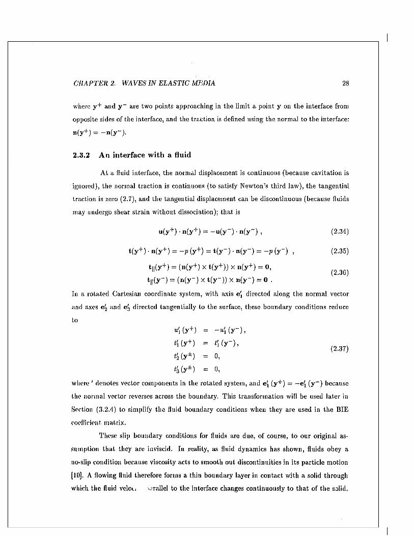
C H A P TE R 2. W AVES IN E L A S T IC M ED IA 28
where y+ and y~ are two points approaching in the lim it a point y on the interface from
opposite sides of the interface, and the traction is defined using the normal to the interface:
n(y+) = -n (y -) .
2.3.2 An interface with a fluid
A t a fluid interface, the normal displacement is continuous (because cavitation is
ignored), the normal traction is continuous (to satisfy Newton’s third law), the tangential
traction is zero (2.7), and the tangential displacement can be discontinuous (because fluids
may undergo shear strain w ithout dissociation); th a t is
u(y+) • n(y+) = —u(y“) • n(y-) , (2.34)
t(y+) • n(y+) = - p (y+) = t(y") • n(y“) = - p (y~) , (2.35)
t||(y+) = (n(y+) X t(y+)) X n(y+) = 0, ^
t||(y~) = (n(y-) X t(y-)) x n(y“) = 0 .
In a rotated Cartesian coordinate system, with axis e) directed along the norm al vector
and axes e '2 and e3 directed tangentially to the surface, these boundary conditions reduce
to
«5(y+) = - « i ( y “),
‘U y + ) = t U y (2.37)<2 (y*) = °»
^(y*) = °.where ' denotes vector components in the rotated system, and e( (y+ ) = - e ) (y ~ ) because
the norm al vector reverses across the boundary. This transform ation will be used la ter in
Section (3.2.4) to simplify the fluid boundary conditions when they are used in the BIE
coefficient matrix.
These slip boundary conditions for fluids are due, of course, to our original as
sumption th a t they are inviscid. In reality, as fluid dynamics has shown, fluids obey a
no-slip condition because viscosity acts to smooth out discontinuities in its particle motion
[10]. A flowing fluid therefore forms a thin boundary layer in contact w ith a solid through
which the fluid veloti wrallel to the interface changes continuously to th a t of the solid,
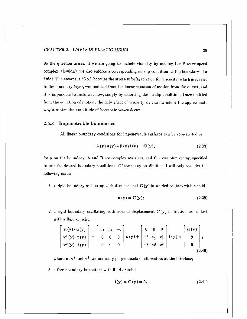
C H A P T E R 2. W A V E S IN E L A S T IC M ED IA 29
So the question arises: if we are going to include viscosity by making the P wave speed
complex, shouldn’t we also enforce a corresponding no-slip condition at the boundary of a,
fluid? T he answer is “No,” because the stress-velocity relation for viscosity, which gives rise
to the boundary layer, was om itted from the linear equation of motion from the outset,, and
it is impossible to restore it now, simply by enforcing the no-slip condition. Once om itted
from the equation of motion, the only effect of viscosity we can include is the approxim ate
way it m akes the am plitude of harmonic waves decay.
2.S.3 Impenetrable boundaries
All linear boundary conditions for im penetrable surfaces can be represented as
A ( y ) u ( y ) + B ( y ) t ( y ) = C ( y ) , (2.38)
for y on the boundary. A and B are complex m atrices, and C a complex vector, specified
to suit the desired boundary conditions. Of the many possibilities, 1 will only consider the
following cases:
1. a rigid boundary oscillating with displacement C (y) in welded contact with a solid
u (y ) = C ( y ) ; (2.39)
2. a rigid boundary oscillating with norm al displacement 6'(y) in frictionless contact
w ith a fluid or solid
n (y) • U (y) Til ra2 «-3 0 0 0 ’ c ( y )
v1 (y) • t (y) = 0 0 0 «(y) + v\ V2 t(y) = 0
, v 2(y) - t (y)_ 0 0 0 _v\ vl v* 0(2.40)
where n, v 1 and v 2 are m utually perpendicular unit vectors a t the interface;
3. a free boundary in contact with fluid or solid
t(y) = C(y) = 0. (2.4 J)
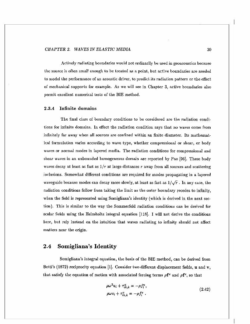
C H A P TE R 2. W AVES IN E L A S T IC M E D IA 30
Actively radiating boundaries would not ordinarily be used in geoacoustics because
tbe source is often small enough to be trea ted as a point, bu t active boundaries are needed
to model the performance of an acoustic driver, to predict its rad iation p a tte rn or the effect
of mechanical supports for example. As we will see in C hapter 3, active boundaries also
perm it excellent numerical tests of the BIE m ethod.
2.3.4 Infinite domains
T he final class of boundary conditions to be considered are the radiation condi
tions for infinite domains. In effect the radiation condition says th a t no waves come from
infinitely far away when all sources are confined within an finite diam eter. Its m athem at
ical form ulation varies according to wave type, whether compressional or shear, or body
waves or norm al modes in layered media. The radiation conditions for compressional and
shear waves in an unbounded homogeneous domain are reported by Pao [96]. These body
waves decay at least as fast as 1/r a t large distances r away from all sources and scattering
inclusions. Somewhat different conditions are required for m odes propagating in a layered
waveguide because modes can decay more slowly, a t least as fast as 1 /y /r . In any case, the
radiation conditions follow from taking the limit as the outer boundary recedes to infinity,
when the field is represented using Somigliana’s identity (which is derived in the next sec
tion). This is similar to the way the Sommerfeld radiation conditions can be derived for
scalar fields using the Helmholtz integral equation [118]. I will not derive the conditions
here, but rely instead on the intuition th a t waves radiating to infinity should no t affect
m atters near the origin.
2.4 Som igliana’s Id en tity
Somigliana’s integral equation, the basis of the BIE m ethod, can be derived from
B etti’s (1872) reciprocity equation [1]. Consider two different displacement fields, u and v ,
tha t satisfy the equation of motion with associated forcing term s p i u and p f v, so th a t
p u 2Ui + T?jf. i. = - p ft1,’ (2.42)
W + Tik,k = ~Pf i ■
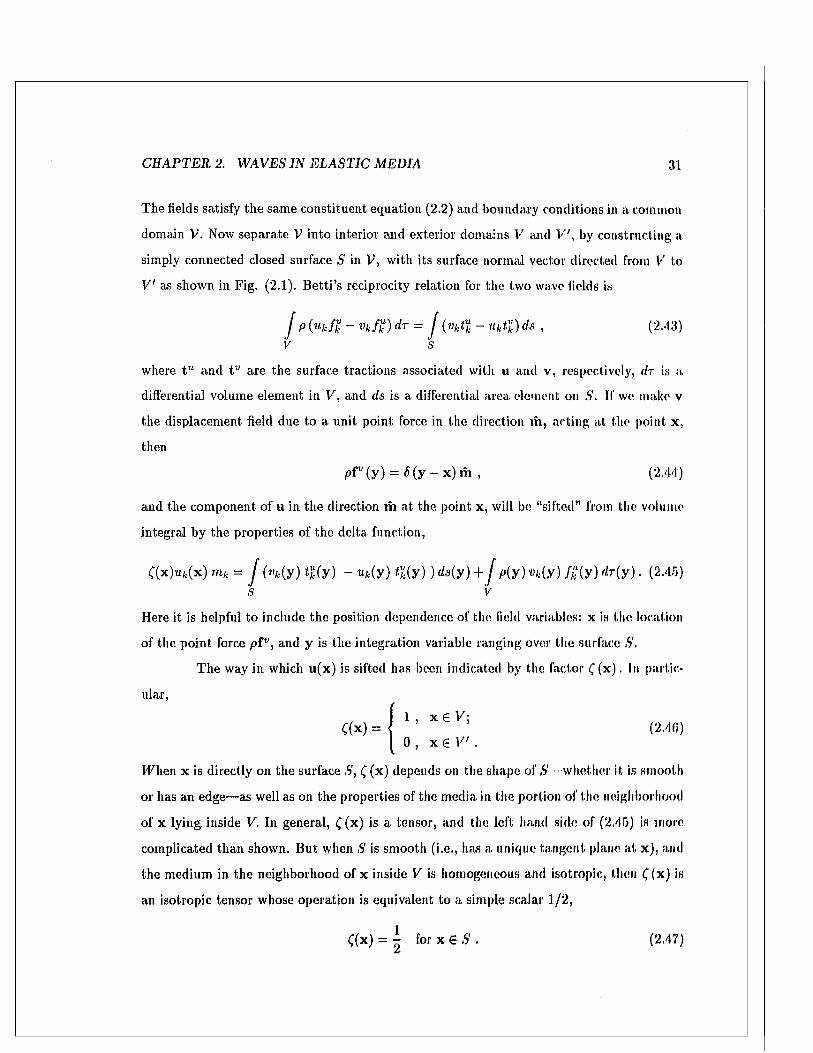
C H A P T E R 2. W A V E S IN E L A S T IC M ED IA 31
The fields satisfy the same constituent equation (2.2) and boundary conditions in a. common
domain V. Now separate V into interior and exterior domains V and W, by constructing a
simply connected closed surface S in V, with its surface normal vector directed from V to
V ' as shown in Fig. (2.1). B e tti’s reciprocity relation for the two wave fields is
J P (Ukfk ~ n f k ) dr = J (vkt l - uktvk) ds , (2.43)V s
where t“ and t v are the surface tractions associated with u and v, respectively, dr is a
differential volume element in V, and ds is a differential area element on S. If we make v
the displacement field due to a unit point force in the direction m, acting at the point x,
then
pfv (y) = 6 (y - x) m , (2.44)
and the com ponent of u in the direction m a t the point x, will be “sifted” from the volume
integral by the properties of the delta function,
C(x)«jfc(x) mk = j (vk(y) t%(y) - uk(y) tvk{y) ) ds(y) + j p(y) vk(y) f%(y) dr(y). (2.45) S V
Here it is helpful to include the position dependence of the field variables: x is the location
of the point force pf v, and y is the integration variable ranging over the surface S.
The way in which u(x) is sifted has been indicated by the factor £ (x) . In partic
ular,
' 1 , x e F ;C(*) = (2.40)
0 , x 6 V ' .
IFhen x is directly on the surface S, C (x ) depends on the shape, of S whether it is smooth
or has an edge—as well as on the properties of the m edia in the portion of the neighborhood
of x lying inside V. In general, ( (x) is a tensor, and the left hand side of (2.45) is more
complicated than shown. B ut when S is smooth (i.e., lias a unique tangent plane at x ), and
the medium in the neighborhood of x inside V is homogeneous and isotropic, then ( (x ) is
an isotropic tensor whose operation is equivalent to a simple scalar 1/ 2,
C(x) = | for x 6 5 . (2.47)
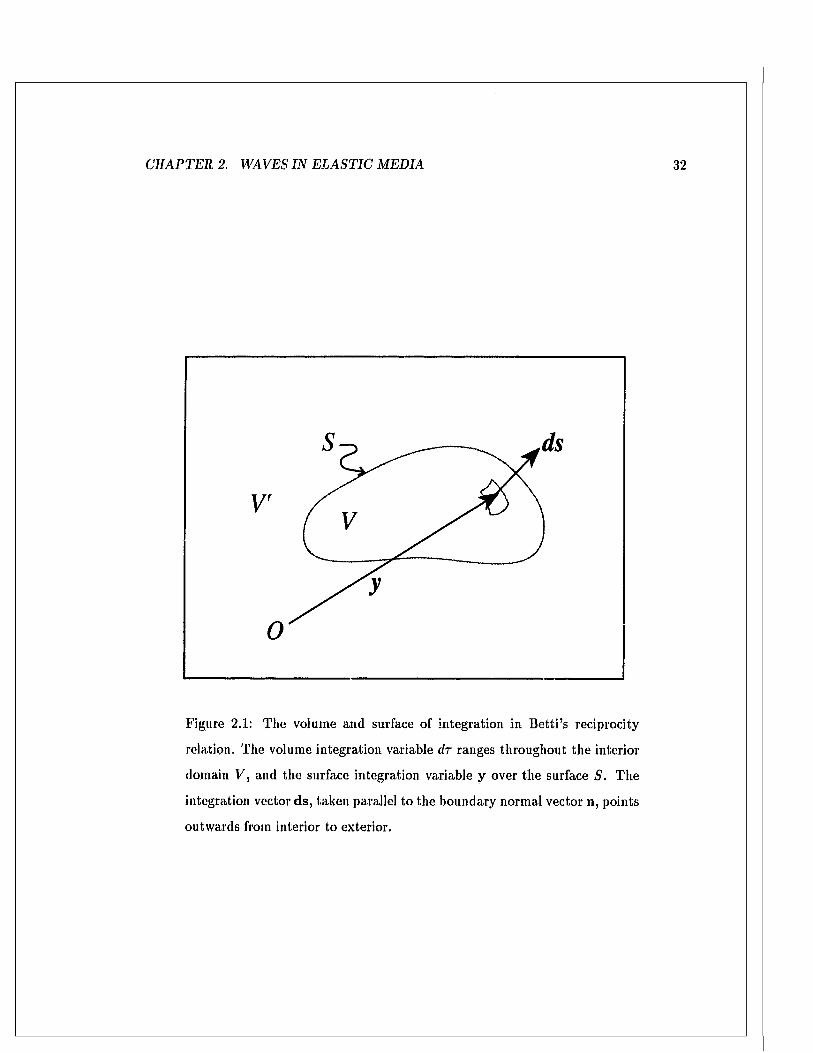
CHAPTER. 2. W AVES IN E L A S T IC M ED IA 32
o
Figure 2.1: The volume and surface of integration in B e tti’s reciprocity
relation. The volume integration variable dr ranges throughout the interior
domain V , and the surface integration variable y over the surface S. The
integration vector d s , taken parallel to the boundary norm al vector n , points
outwards from interior to exterior.
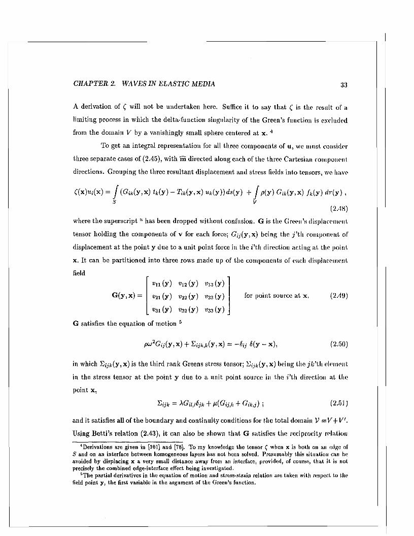
C H A P T E R 2. W A V E S IN E L A S T IC M EDIA 33
A derivation of £ will not be undertaken here. Suffice it to sa,y th a t ( is the result of a
limiting process in which the delta-function singularity of the G reen’s function is excluded
from the domain V by a vanishingly small sphere centered a t x . '•
To get an integral representation for all three components of u , we m ust consider
three separate cases of (2.45), with m directed along each of the three Cartesian component
directions. Grouping the three resultant displacement and stress fields into tensors, we have
where the superscript u has been dropped without confusion. G is the G reen’s displacement
displacement at the point y due to a unit point force in the i ’th direction acting at the point
x. It can be partitioned into three rows m ade up of the components of each displacement
in which E y * (y ,x ) is the third rank Greens stress tensor; E y * (y ,x ) being the j k ’t h element
in the stress tensor a t the point y due to a unit point source in the ii’th direction at the
point x ,
and it satisfies all of the boundary and continuity conditions for the total domain V = V + V',
Using B e tti’s relation (2.43), it can also be shown th a t G satisfies the reciprocity relation
4Derivations are given in [101] and [78], To my knowledge the tensor ( when x is both oil an edge of S and on an interface between homogeneous layers has not been solved, Presumably this situation can be avoided by displacing x a very small distance away from an interface, provided, of course, th a t it is not precisely the combined edge-interface effect being investigated,
6The partia l derivatives in the equation of motion and strcss-strain relation are taken with respect to the field point y , the first variable in the argum ent of the Green’s function,
C(x)«i(x) = J (Gik(y ,x ) tk( y ) - T ik( y , x ) uk( y ) ) d s ( y ) + j />(y ) (?<*(y ,x ) f k { y ) rfr(y) ,s V
(2.48)
tensor holding the components of v for each force; Gij(y ,x ) being the y ’th component of
for point source at x.
G satisfies the equation of m otion 5
p u 2G i j ( y ,x ) + %ijk,k( y , x ) = - S y 6 (y - x ), (2.50)
(2.51)
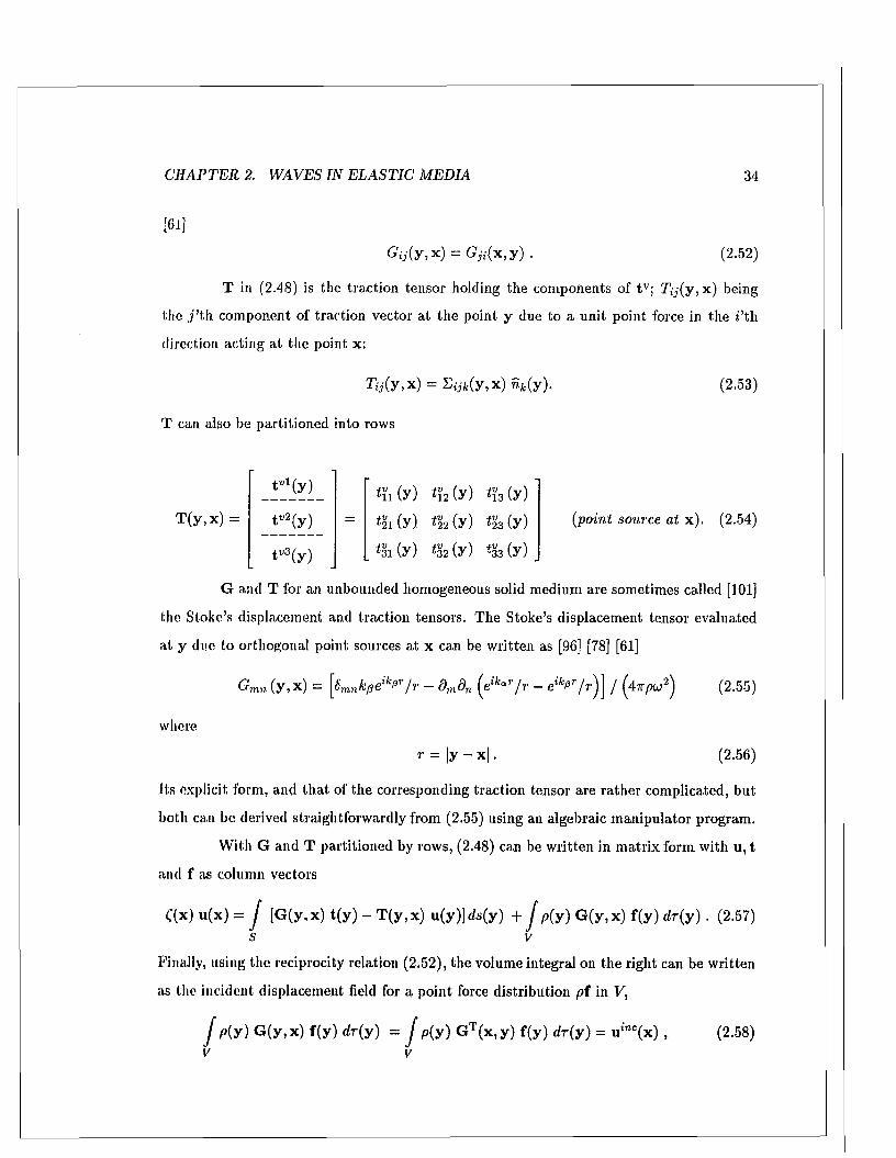
C H A P TE R 2. W AVES IN E L A S T IC M ED IA 34
[61]
Gij(y , x ) = G ji(x , y ) . (2.52)
in (2.48) is the traction tensor holding the components of t v\ T{j(y, x ) being
the j ’th com ponent of traction vector at the point y due to a unit point force in the i ’th
direction acting at the point x:
Tij{y ,x ) = Eijk(y , x) n k(y).
T can also be partitioned into rows
(2.53)
tul(y) i vu (y) t h (y) *13 (y)T (y ,x ) = t"2(y) = *21 (y) *22 (y) *23 (y)
r s (y ) . *31 (y) *32 (y) *33 ( y ) .
(point source at x ). (2.54)
G and T for an unbounded homogeneous solid medium are sometimes called [101]
the Stoke’s displacement and traction tensors. The Stoke’s displacement tensor evaluated
at y due to orthogonal point, sources at x can be w ritten as [96] [78] [61]
Gmn (y,x) = [Smn^i3 GlkPr/ r - dmdn (etkar/ r - e ^ V 7')] / (47rp u 2) (2.55)
w lie re
r = |y - x | . (2.56)
Its explicit form, and th a t of the corresponding traction tensor are ra ther complicated, but
both can be derived straightforw ardly from (2.55) using an algebraic m anipulator program.
W ith G and T partitioned by rows, (2.48) can be w ritten in m atrix form with u, t
and f as column vectors
C(x) u(x) = J [G(y,x) t(y) - T(y,x) u(y)]ds(y) + J p(y) G(y,x) f(y) dr(y) . (2.57)S V
Finally, using the reciprocity relation (2.52), the volume integral on the right can be w ritten
as the incident displacement field for a point force distribution p i in V,
J p(y) G(y,x) f(y) dr(y) = J p(y) GT(x,y) f(y) dr(y) = uinc(x) , (2.58)
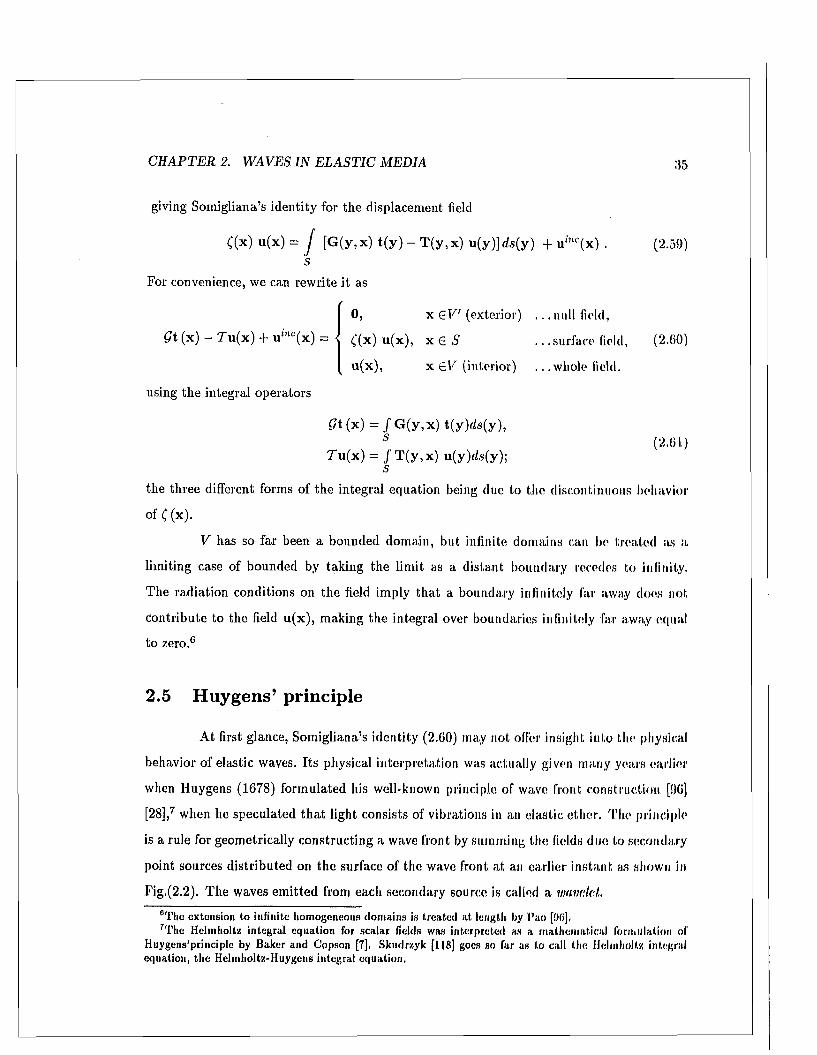
C H A P TE R 2. W A V ES IN E L A S T IC M ED IA 35
giving Somigliana’s identity for tlie displacement field
C(x)u(*) = / (G(y,x) t ( y ) -T (y ,x ) u(y)]ds(y) + uinc(x) . (2.59)s
For convenience, we can rewrite it as
{0 , x e V ' (exterior) . . . null field,
C(x) u (x ) , x € S . . .surface field, (2.60)
u (x ) , x e V (interior) . . . whole field.
using the integral operators
Qt (x ) = / G (y ,x ) t ( y )d s (y ) ,s (2.61)
T u (x ) = / T ( y , x ) u(y)f/s(y);5
the three different forms of the integral equation being due to the discontinuous behavior
of C (x).
V has so far been a bounded domain, but infinite domains can be treated as a
limiting case of bounded by taking the lim it as a distant boundary recedes to infinity.
The radiation conditions on the field imply tha t a boundary infinitely far away does not
contribute to the field u (x ), making the integral over boundaries infinitely far away equal
to zero.6
2.5 H u ygen s’ principle
A t first glance, Somigliana’s identity (2.60) may not offer insight into the physical
behavior of elastic waves. Its physical interpretation was actually given many years earlier
when Huygens (1678) form ulated his well-known principle of wave front construction (96]
[28],7 when he speculated th a t light consists of vibrations in an elastic other. The principle
is a rule for geometrically constructing a wave front by summing the fields due. to secondary
point sources d istributed on the surface of the wave front a t an earlier instan t as shown in
Fig.(2.2). The waves em itted from each secondary source is called a wavelet.
6The extension to infinite homogeneous dom ains is treated a t length by Pao [DO],7The Helmholtz integral equation for scalar fields was interpreted as a m athem atical formulation of
Huygens’principle by Baker and Copson [7], Skudrzyk [118] goes so far as to call the Helmholtz integral equation, the Helmholtz-Huy gens integral equation.
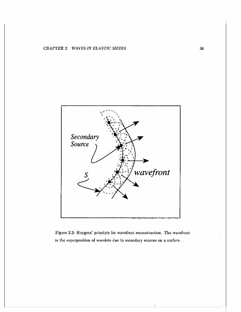
C H A P TE R 2. W AVES IN E L A S T IC M ED IA 36
Secondary Source ^
wavefront
Figure 2.2: Huygens’ principle for wavefront reconstruction. T he wavefront
is the superposition of wavelets due to secondary sources on a surface.
C H A P T E R 2. W AVES IN E L A S T IC M ED IA 37
Huygens’ principle involves two conjectures implicit in (2.60). The first is tha t
the displacement field is the superposition of wavelets originating from a distribution of
secondary sources on a surface, plus any direct waves em itted from actual sources. This be
comes evident when we view the integrands of the operators (2.61) as two different; wavelets,
where the field variables u and t play the role of secondary source strengths on the surface
S, and the boundary integral is their superposition taken in the lim it of a continuous source
distribution:
s im ple wavelet =*> G (y ,x ) t (y ) r/.s(y) ,
complex wavelet =J> - T ( y ,x ) u (y ) ils(y) , (2.62)
direct waves f r o m source => u mc ( x ) .
The surface source distributions are often called potential layers [78]. They are an extension
of the monopole and dipole potential layers of a scalar wave theory [68].
The second conjecture is th a t the behavior of the wavelet propagation is not af
fected by w hat lies in the domain excluded by the boundary 5. This is evident because
the G reen’s te rro rs , G and T , governing the wavelet propagation are determined without
reference to the boundary S. Hence the wavelets always radiate as if into the entire domain
V, regardless of w hat m ay lie in the exterior domain V'.
We can m ake full use of Huygens’ principle when solving scattering problems. Ap
plying the first conjecture, we can subdivide the domain of our scattering problem into any
num ber of subdom ains in which the displacement field can be expressed as the superposition
of wavelets from secondary sources on its boundary. A subdomain can have any size because
the wavelet integral (2.60) is exact. Applying the second, we see tha t a subdomain only
interacts with its neighbors through the wavelet source strengths u and t along a common
boundary, so we can trea t it as a volume element embedded in one scattering problem or
another, b u t whose integral operators in the boundary integral equation remain the same
for all problems. This m odular interchangeability of subdomains is central to the new in
direct BIE m ethod and to numerical tests. I t also implies th a t we have some freedom in
choosing the G reen’s function for the wavelets in a subdomain: it m ust satisfy the equation
of motion and boundary conditions everywhere inside, but it can satisfy any conditions at
points outside the boundaries. In a subdom ain consisting of a homogeneous medium, for
C H A P TE R 2. W AVES IN E L A S T IC M ED IA 38
instance, we can use the G reen’s function for the corresponding unbounded homogeneous
domain because it satisfies the equation of motion everywhere inside the subdom ain .8
In summary, Huygens’ principle, formulated m athem atically using Somigliana’s
identity, allows us to subdivide a complicated domain for which the G reen’s function is
intractable, into simpler domains in each of which the G reen’s function is tractable. W ithin
each subdom ain, the displacement field is represented by the superposition of the wavelet
fields, and adjacent subdomains are coupled together through field continuity conditions
applied at their common boundaries. In terms of Huygens’ principle, the BIE m ethod
proceeds in two steps: 1) to com pute the wavelet source strengths u and t on the boundary
of each subdomain in the scattering problem; and 2) to com pute the displacement field at
any point within a subdom ain by wavelet superposition.
2.6 T he boundary integral perspective
When a dom ain is subdivided, we quickly run into confusion between interior and
exterior, for the interior of one subdom ain lies in the exterior of another. The problem is
compounded by the three possibilities in (2.60) th a t depend on the location of x relative
to the boundary of the subdom ain under consideration. We must, be clear about which
enclosing surface we are integrating over, which G reen’s tensors are to be used in the
integrand, and which side of the boundary is to be interior and which the exterior domain.
1 call this the perspective of the integral equation. Switching the perspective changes the
integral equation completely.
Suppose, for instance, th a t we have a single homogeneous scattering object em
bedded in an oceanic, waveguide, One obvious way—no doubt the best way—of subdividing
the domain is to use the surface of the scattering object itself as the integration boundary
separating the infinitely large layered domain from the finite scattering object. From the
perspective of the host waveguide, then, the interior domain is the infinite region outside
Hie scattering object, whereas, from the perspective of the scattering object, the interior do
main is the homogeneous region within it. And from the perspective of the host waveguide,
"The G reen's functions for an unbounded homogeneous fluid and solid domains can be found in the literature [DC] [78] [61] [91] [101].
C H A P T E R 2. W AV E S IN E L A ST IC M ED IA 39
the simplest G reen’s function is tha t of the undeformed waveguide (the scattering object
being entirely excluded by the integration boundary), whereas, from the perspective of the
embedded inclusion, the simplest Green’s function is tha t of an unbounded homogeneous
medium having the same elastic param eters as the scattering object (the host, waveguide be
ing entirely excluded by the integration boundary). The boundary integral is “told” which
is the interior for each perspective by the direction of the normal vector on the bound
ary. Following the convention used in B etti’s reciprocity theorem, the normal vector always
points outw ards from the interior domain.
2.7 D eterm in ing th e boundary fields
Having subdivided the scattering problem into domains for which we can compute
suitable G reen’s functions, it remains to decide, which of the three integral formulations
in Somigliana’s iden tity— the null-, surface-, or whole-field equation can be used together
with the continuity and boundary conditions to determine the elastic field on the boundaries,
Consider first the null-field equation in (2.60). The unknown field variables, u and
t , only appear within the integrands making it an integral equation of the first kind, which
as a rule are disastrously unstable .9 Nevertheless equations of the first-kind have been used
with some success [123], so let us include it as a possible candidate, for determ ining the
boundary field and use it with caution.
Next consider the surface-field equation in (2.60). The unknown boundary dis
placement u appears both inside and outside the integral, whereas the fraction t only
appears inside the integral. Thus, we might say the. surface-field equation is of the second
kind in u, but of the first kind in t, If' we consider a traction-free boundary, for exam
°Arfken [<1] explains the instability this way: fn an equation of the first kind
<fi{x)= I I \ ( x , y ) f ( y ) <l y = l \ f ( x ) ,
is insensitive to small variations in K and / because integration is a “sm oothing” operator, whereas / is very sensitive to variations in <p. When K and are approximated numerically, the solution
will therefore be sensitive to small numerical errors in y>, which means th a t A '"1 m ust be unstable small numerical errors are magnified and accuracy is lost.
C H A P T E R 2. W AVES IN E L A S T IC M ED IA 40
pic, which is typically used in seismology for scattering from surface topology [67] [92],
then t = 0 from the outset, giving an equation strictly of the second kind in u. B ut at a
rigid-welded boundary, u = 0 from the outset, giving an equation of the first kind in t.
As a rule, equations of the second kind have excellent numerical stability ,10 though
on occasion their solution m ay become nonunique, as shown by the Fredholm theory of
integral equations.11 The problem is well known in scalar wave theory, for it occurs at
isolated critical frequencies in the Neumann and Dirichlet boundary value problems, and a
variety of remedial measures have been developed [29] [106] [22]. In our case, however, the
mixed natu re of the surface-field equation—part first and second kind—raises doubts about
its overall stability. Perhaps bo th the numerical instability which plagues the solution of
equations of the first kind, and the occasional nonuniqueness problem of the equations of
the second kind, may trouble the numerical solution. The question has apparently no t been
raised in the literature, and I am not in a position to resolve it here, but until it is resolved,
we m ust proceed cautiously; careful testing is needed for the solution to any scattering
problem.
Another numerical difficulty with the surface-field equation invariably arises when
com puting the Cauchy Principal Value (CPV ) because the integrand is singular a t the
com putation point x £S due to the singularity in the G reen’s function. This can be a
difficult task, especially for layered waveguides whose G reen’s function cannot be w ritten in
simple closed form and is also slowly convergent in the very near field. I will use an indirect
integration method to avoid both problems a t once.
It should be noted th a t Somigliana’s identity could be converted to an equation of
the second kind in t by first differentiating it to construct an integral representation for the
strain tensor (2.1), then using Hooke’s law (2.2) to get the corresponding stress tensor. The
10!n equations of the second kind
<p[x) = J K ( x , y ) f (y) dy + A/ (x) = K f ( x ) + A/ ( x ) ,
the A /(x ) term generally leads to diagonal dominance, hence stability, in the numerical system of equations th a t determ ine / ( x ) ,
’ 'T h e Fredholm theory for integral equations establishes the existence and uniqueness of the solution to an integral equation of the second kind [12!)]. T he Riesz theory for com pact operators is the extension to integral equations having weakly singular kernels [105][29].
C H A P TE R 2. W A V E S IN E L A S T IC M ED IA 11
equivalent lias been done more simply in scalar wave theory to solve (Dirichlot) problems
with zero-pressure boundary conditions, converting the Helmholtz integral equation from
the second kind in pressure, to the second kind in normal velocity [22]. Where the original
equation is weakly singular [29], however, the modified is hypersingular, which presents
still greater num erical complications for the BIE method, except when used with the zero-
pressure boundary conditions. In the vector theory, the ensuing hypersiugular integrals
would ordinarily be encountered in all problems except scattering from im penetrable rigid
inclusions. It may be possible to avoid troublesome hypersingularities using the indirect
integration m ethod I propose, though I do not explore the possibility here.1’2
Finally, consider the whole fie! 1 equation in (2.60) as a means for deriving the
unknown boundary field. As it stands, the equation cannot be used because it introduces
yet another unki.own function, the displacement field in the interior domain, u (x ) for x e l ' .
The interior displacement field m ust somehow be eliminated first, possibly by relating the
field at x to the field on the boundary in an approxim ate way.13
2 .7 .1 A c o m b in e d e q u a t io n m e t h o d
To overcome occasional nonuniqueness problems in equations of the second kind
in the Neumann problem in acoustics, Schenck [106] used both the surface- and null field
equations together in his combined equation method. In effect, the null-field equation
overdeteimines the num erical solution, forcing a unique best-fit result when the solution Lo
the surface-field equation on its own is nonunique. Going one step further, the combined
method can be viewed as a generalization of BIE methods tha t are so often based exclusively
on cither one equation or the other. One could, for example, a ttem p t a solution based
strictly on either the surface- or null-field equation, or combine them in varying degrees
12I have not come across any references to the modified integral representation for the stress tensor in the literature.
l3While a t the SACLANT C enter in be Spezia Italy, I developed a simple finitc-difference scheme to do ju s t th a t for scalar fields in two-dimensional fluid media, By placing the com pulation point x very close to the boundary, a single finite difference slop could accurately connect the field a t x to the field on the boundary in its im m ediate vicinity; a complete finite-dilference treatm ent of the interior volume was not rccpiired, The modified equation has the stable properties of the surface-field equation with the singularity in the integrand favorably weakened since x is no longer on the boundary. Unfortunately, I have no t been able to extend the method to vector fields.
C H A P TE R 2. W AVES IN E L A S T IC M ED IA 42
to overdetermine, and possibly stabilize, an otherwise unstable solution. The freedom to
experiment with combinations this way would be an advantage, especially as numerical
stability is not assured. In the next chapter I develop a flexible combined m ethod th a t can
use any combination of the surface- and null-field equations.
43
C h a p t e r 3
The indirect BIE m ethod
We have seen how the domain of a scattering problem can be subdivided into sub
domains (volume elem ents), each with its own perspective for the boundary integral equa,-
tion. T he BIE m ethod continues in two steps: 1) by computing the field on the boundaries
of the subdom ains (the Huygens’ wavelet strengths); and 2) by computing the displacement
field at any point off the boundary, again using Somigliana’s identity (the superposition of
wavelets). In this chapter I take up the numerical details. The m ethod is dem onstrated lor
scattering by spheres, for which benchmark analytic solutions can be computed by separa
tion of variables m ethods. Examples involving layered waveguides m ust wait until Chapter
7, after the requisite G reen’s function is developed in C hapters 4, 5 and 6.
3.1 N um erical approxim ation o f th e boundary integral
The num ber of points on the boundary where u and t must be com puted is infinite,
so the first numerical approxim ation is to reduce the continuous domain to a finite number
of points, called nodes, by dividing the boundary into small elements on which the field
can be in terpolated from its values at the nodes. The elements cannot be too large or the
interpolation becomes inaccurate, nor too small or the dem ands upon com puter memory
become excessive.
A boundary element can be m apped to a square in a two-dimensional coordinate
system £ = [£t,£2]T ; _ 1 < £1,2 < +1. When interpolated from its nodes using shape

C H A P TE R 3. TH E IN D IR E C T B IE M ETH O D 44
(3.1)
functions N m (£), the field at a point x (£) on the n ’th boundary element is [8]
« i(x ) = N m (Z)u?m ,
t{ (x ) = N m (£) tfm .
urn = [u vnnu2 mi uz m f and are the displacement and normal traction
at the '/n’th node on the n ’th boundary element, and sum m ation over m is implied. M any
different shape functions for boundary elements can be used. In my own BIE program I use
quadrilateral boundary elements as shown in Fig. (3.1), with triangular elements treated
as degenerate quadrilaterals. Q uadratic shape functions accurate to second order can be
constructed using a nine-node interpolation scheme [132] [79]
N i ( 0 = 26 (6 - 1) K 2 (& - i ) ,
N 2 ( t ) = ( i - t f ) 2 2 - i ) ,
t f 3 ( 0 = (6 . + 1) (6 - i ) ,
n 4 ( 0 = i 6 ( a + i ) (1 -- m
K i t ) = K i ( ^ + i) ^ 2 ( 6 + 1) ,
N e ( 0 = (1 - &) ^ 2 ( 6 + 1) ,
N 7 {t) = ( 6 - 1) 5 6 (6 + i)>
N s ( 0 = (f i - 1) (1 -- 3 ) >
iV9 ( 0 = (1 - ) (1 -- 3 ) •
(3.2)
In general, the numerical approxim ation for the integral operators (2.61) can be
written as
where
QM ( x )
T « i( x )
Gijm (X) tjm i
V j m (x ) Ujm ,
G$m (x ) = f G i j f y ( ( ) , x ] N m (( ) J ( 0 « 2 ,s»
V n (x) = / W 0 . x ] ^ ( e W l < i f 2 .Sn
(3.3)
(3.4)
Here ./ (£) is the Jacobian for the transform ation from £ to the local coordinates of the
element [8], and S n is the surface of the n ’th boundary element. and T$m are bound
ary integral coefficients th a t depend on 1) the G reen’s function for the perspective of the
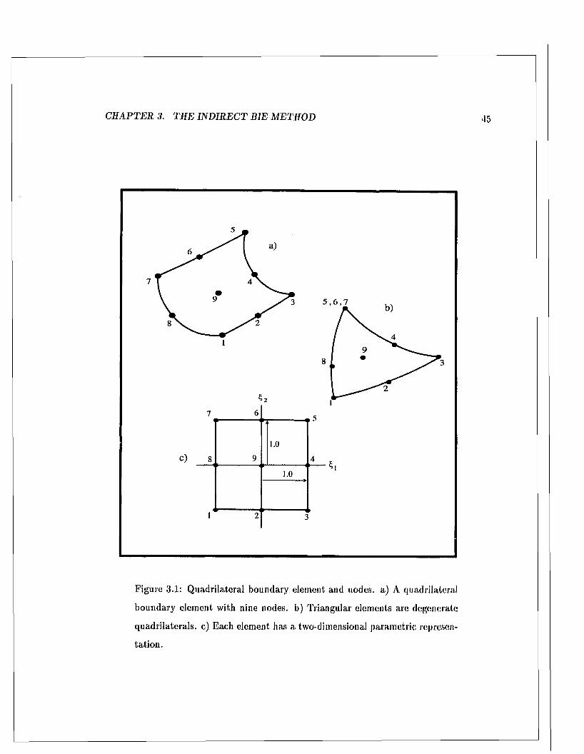
C H A P T E R 3. T H E IN D IR E C T BIE M ETH O D
Figure 3.1: Q uadrilateral boundary element and nodes, a) A quadrilateral
boundary element with nine nodes, b) Triangular elements are degenerate
quadrilaterals, c) Each element has a two-dimensional param etric represen
tation.
C H A P T E R 3. T H E IN D IR E C T B IE M E T H O D 46
equation, 2) the shape of the boundary element, and 3) the com putation point x; but they
do not depend on the boundary or continuity conditions applied to the field. Substituting
the approxim ate operators into (2.60) gives
0 ... null-field,
( (x) N m, (x) uf^i — surface-field, (3.5)
Ui (x) ... whole-field.
Gtjm (x ) ^ m - ^ m ( x ) « ^ + « r ( x )
In the surface-field equation, n' is the boundary element containing x, and the sum m ation
over w! is over the nodes on ju st th a t element.
Nodes often touch several boundary elements because they lie on the perim eter of
an element. The double indices ^ can therefore be replaced by a single index m ranging
over all the nodes by switching to a global num bering scheme for all d istinct nodes
7i ( m )
Gijm (x ) = X) Gtjm (x ) )71=1
(3.6)71(771)
Tijm ( x ) = ^ 7 7 7 1 ( x ) •71=1
n (m ) is the num ber of boundary elements in contact w ith the m ’tli node. Equation (3.5)
therefore becomes
Gijm (x ) f.j'771 % jm (x ) *1)771 + u i (x )
0 ... null-field,
£ (x) !Vm/ (x) Uimi ... surface-field, (3.7)
U{ (x) ... whole-field.
This numerical approxim ation to the whole-field equation is perhaps the way we usually
think of Huygens’ principle: the field u(x) is the superposition of m boundary wavelet
sources d istributed on a boundary plus the incident field u mcdue to sources in the interior
dom ain.
3.2 A flexib le com bined equation m ethod
As mentioned in Section (2.7), the unknown boundary field Ujm and t jm can be
com puted using both the surface-field equation and the null-field equation. Here I describe
C H A P T E R 3. T H E IN D IR E C T B IE M E TH O D 4 7
a flexible num erical m ethod th a t perm its any combination of the two.
3.2.1 Surface-field equations
If x is placed at the m ’th node, then uj (x) = uj (x,„) = u jm , which occurs
on bo th sides of the surface-field equation (3.7). By placing x successively at each of
the nodes, we can in principle construct a full system of equations in terms of u jm and
t jm; one vector equation arising from each node on the boundary; lvence twice as ma;ny
unknowns as equations. More generally, com putation points can be placed anywhere on
the boundary using interpolation as shown on the right side of (3.7). Thus, any num ber of
com putation points can be placed on the boundary giving any num ber of equations, though
additional points beyond the num ber of nodes do not help to determ ine the solution because
the additional equations approxim ate linear combinations of the others. The freedom to
place surface nodes anywhere on the boundary—especially away from the perim eter of the
boundary elem ents—is an advantage because we can avoid com puting a complicated sifting
factor C for nodes on edges. It is also helpful in the new indirect BIE method as we will see.
3.2.2 Null-field equations
Null-field equations have the same form as surface-field equations, except the right-
hand side of (3.7) is identically zero. Here again, we can construct any number of equations
by choosing any num ber of com putation points x in the exterior domain of the perspective.
As m entioned in Section(2.7), the null-field equation is likely to suffer from insta
bility because i t is an equation of the first kind. Instability sets in as the boundary elements
are m ade smaller for improved accuracy. Increasing the node density eventually makes the
m atrix coefficients for a node roughly equal to a scalar multiple of the same coefficients for a
nearby node, which in tu rn makes the columns in the m atrix linearly dependent. A ttem pts
to im prove accuracy m ay therefore make it worse.1 Null-field equations have been used
successfully nonetheless [123]. Notice th a t a greater degree of error due to instability can
*The same problem does not occur in equations of the second kind because its distinctive term the unknown variable appearing outside the integral—is independent of the clem ent size, ensuring diagonal dominance as the elem ent size is reduced since the m agnitude of tin m atrix coefficients Oipn and decrease roughly in proportion to the elem ent area.
C H A P T E R 3. T H E IN D IR E C T B IE M E TH O D 48
be tolerated in scattering than if the boundary field were itself the final objective, for the
boundary field is only an interm ediate step towards the field at points off the boundary,
for which the whole-field equation will tend to sm ooth out irregularities due to instability
provided they are not too large .2 Moreover, there m ay be an optim al boundary element size
th a t is a t once small enough to adequately sample the boundary field by their node spac
ing, and large enough to avoid disastrous instability. A t any ra te , it is clear th a t null-field
equations must be used with caution and careful testing.
3.2.3 Combined equation m ethod
To fully determ ine the boundary field, additional equations m ust come from the
boundary conditions (2.38) and the continuity equations (2.32 to 2.36) applied to the field
at eacli node. Clearly these play an im portant role because they assemble the subdom ains of
the scattering problem together; the continuity conditions connecting domains across their
penetrable boundaries, and boundary conditions prescribing the behavior a t im penetrable
boundaries. Unlike the integral equations, the boundary and continuity equations are sparse
because each pertains to ju s t one or two nodes ra ther th an to m any nodes at once.
A general algorithm to m anage the continuity and boundary conditions is difficult
to write, especially in layered m edia where an inclusion m ay be in contact w ith fluids in
some places and solids in others, or when a scattering problem includes several objects
in contact with the host medium as well as with each other, perhaps with one object
completely embedded within another. Boundary conditions are also needed whenever a
scattering inclusion is in contact with a free surface or rigid bottom , or if it is a source
actively radiating energy. Perhaps the simplest approach is to include each boundary and
continuity equation as additional equations in the overall B IE coefficient m atrix . T he final
m atrix equation th a t determ ines the field on all of the boundaries sim ultaneously might
look something like this when there are ju s t two inclusions, perspectives 1 and 2 embedded
^Equations of the first kind are particularly worrisome when the boundary field is of prim ary interest, in the study of dynamic stress concentrations th a t lead to fractures a t a boundary for example.
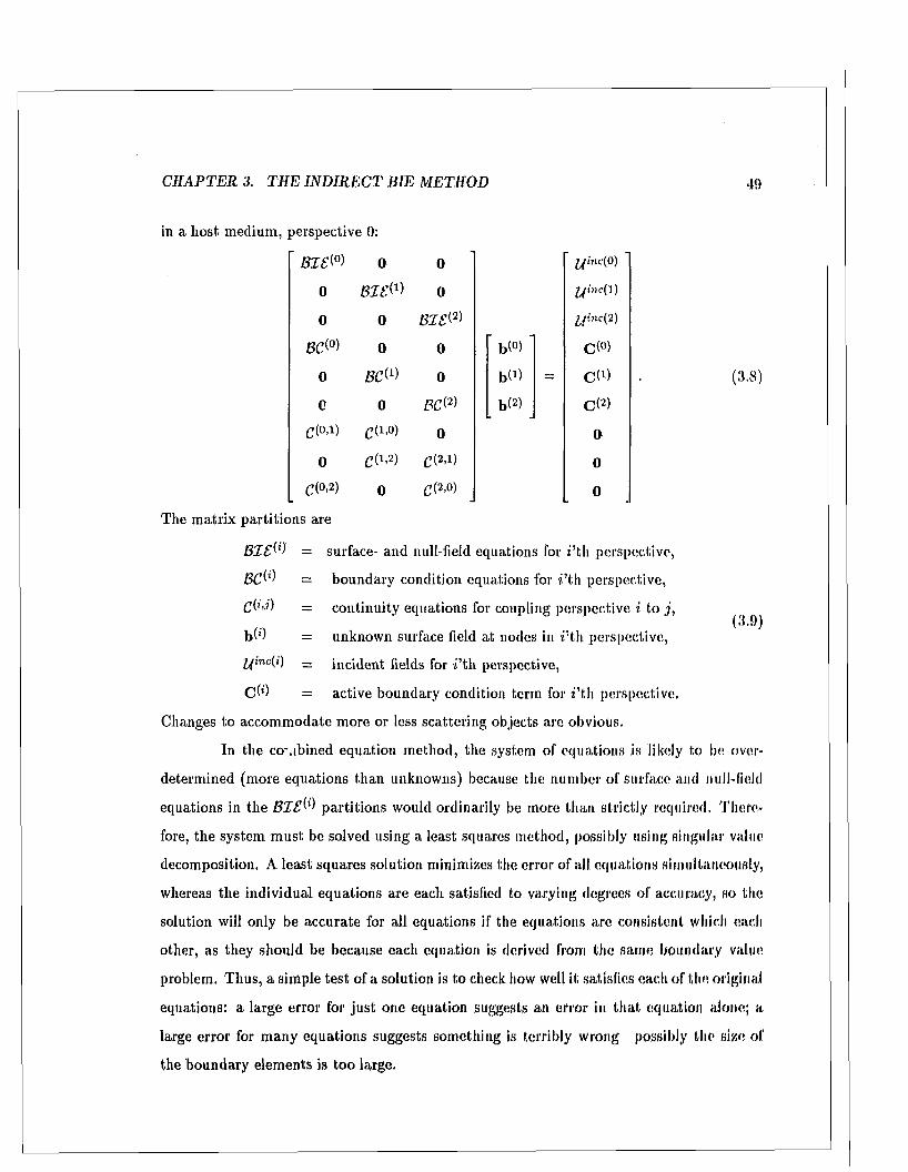
C H A P T E R 3. T H E IN D IR E C T BIE M ETH O D
in a host medium, perspective 0:
49
BISW 0 0 Ifinc(O)
o b x s W o yinc(l)
0 0 B IS& lfinc{ 2)
8C<°) 0 0 ’ b<°)' c(°>0 f id 1) 0 b(l) = CO)C 0 B C W b(2) <d2)
C(°d) d 1-0) o 0
o d 1-2) d 2-1) 0
(7(0,2) 0 d 2'°) 0
(3.8)
BC®
£(*>.))
b «
yinc(i)
c(f)
(3.9)
The m atrix partitions are
B I S W = surface- and null-field equations for i ’th perspective,
= boundary condition equations for i ’th perspective,
= continuity equations for coupling perspective i to
= unknown surface field at nodes in i ’th perspective,
= incident fields for i ’th perspective,
= active boundary condition term for i ’th perspective.
Changes to accom m odate more or less scattering objects are obvious.
In the coMbined equation m ethod, the system of equations is likely to be over
determ ined (more equations than unknowns) because the num ber of surface and null-field
equations in the B I S ^ partitions would ordinarily be more than strictly required. There
fore, the system m ust be solved using a least squares method, possibly using singular value
decomposition. A least squares solution minimizes the error of all equations simultaneously,
whereas the individual equations are each satisfied to varying degrees of accuracy, so the
solution will only be accurate for all equations if the equations are consistent which each
other, as they should be because each equation is derived from the same boundary value
problem. Thus, a simple test of a solution is to check how well it satisfies each of the original
equations: a large error for ju s t one equation suggests an error in th a t equation alone; a
large error for m any equations suggests something is terribly wrong possibly the size of
the boundary elements is too large.
C H A P T E R 3. T H E IN D IR E C T B IE M E TH O D 50
3 .2 .4 C o m p r e s s in g t h e BIE c o e f f ic ie n t m a t r i x
The form of the BIE coefficient m atrix (3.8) is straightforw ard in construction,
even for ra ther complicated problems having fluid and solid media, m ultiple penetrable
inclusions with im penetrable boundaries, and so forth; bu t it is terribly inefficient because
the m atrix is very large (six unknowns, u and t , for every node in every perspective of the
scattering problem), while containing m any sparse partitions (all of the B C ^ and
Before the m atrix equation is solved, the simplest boundary and continuity equations— those
that, merely assign a value to a field variable or couple two variables across a boundary—
should therefore be elim inated using a simple algorithm th a t 1) checks for rows in the
BIE coefficient m atrix with ju st one or two non-zero elements, and then 2) eliminates one
column for each accordingly. The algorithm is simple because it acts w ithout reference to
the particular scattering problem. All of the welded continuity equations between a two
solid m edia can be elim inated this way, reducing the num ber of unknowns by a factor of
two for strictly solid domains in contact. To do the same for fluid media, however, we must
first remove the role of the norm al vector from the boundary and continuity equations for
nodes inside a fluid, by ro tating the boundary displacement and traction vectors to a local
coordinate system having one axis along the boundary normal vector, as m entioned earlier
with regards to equation (2.37). The reduced system of equations can be solved m uch faster
than the unreduced.
A nother reason for compressing the m atrix is to ensure th a t the boundary and
continuity equations are strictly enforced in the solution. Recall th a t the solution of an over
determined system of equations satisfies the system of equations in a least squares sense,
but not every equation considered individually. The boundary and continuity equations will
therefore “drift” when left in the BIE coefficient m atrix: zero traction on a free boundary
will become a. “sm all” traction condition, and welded contact between solids will be slightly
broken for example. The drift will be negligible if the num erical approxim ation of the
boundary value problem is accurate, but noticeable upon careful inspection nonetheless.
BIE programs intended for strictly solid m edia often enforce continuity of displace
ment and traction across a boundary in the way the B I E W partitions are assembled, ra ther
C H A P T E R 3. T H E IN D IR E C T BIE M E T H O D 51
than by including separate continuity equations as in (3.8). From the outset, then, the
displacement field, on the boundary of one. perspective is taken as the displacement field of
another in contact, and the traction field of one taken as the negative traction field of the
other. In effect, the continuity equations in (3.8) are elim inated before constructing the
m atrix, thereby reducing the num ber of unknowns immediately by a factor of two, much
as I propose doing with a m atrix compression algorithm. Hut it is wrong to equate the
displacement on bo th sides of an interface with an inviscid fluid, for th a t enforces no-slip
(welded) continuity a t a fluid boundary, ra ther than the slip condition (See Section (2.3.2)),
which necessarily involves the boundary normal vector.3
3.2.5 A m odular approach to the combined equation m ethod
I follow a m odular approach to the BIE method. One program, computes and
saves the equation coefficients Gijm and %jm for each point x in a list of com putation points
read from a d a ta file. A nother constructs and saves the non-zero partitions of the sparse
boundary condition equations for all the im penetrable elements in a perspective. A third
constructs the to ta l coefficient m atrix by packing the previously saved boundary integral
and boundary condition partitions into the m atrix , while also com puting the incident fields
on the left side of (3.8). It then constructs the coupling equation partitions a t the bottom of
the m atrix, compresses the m atrix, solves for the remaining unknowns using least squares,
decompresses the solution to get the boundary field at every node in every perspective of
the problem, and finally saves the boundary fields. A fourth program computes and saves
the displacement vector at points off the boundaries using the whole-field equation, and a
fifth plots the field in a num ber of ways, using polar plots, grey scale diagrams, and so forth.
The m odular approach has the advantage th a t many com putations do not have to
be repeated every tim e certain aspects of the problem are changed, If the incident field is
changed, by relocating a source for example, only the incident field on the left side of (3,8)
needs to be recomputed. If additional surface- or null-field equations are added later for
3In a scalar theory the boundary normal vector is intrinsic to the field variables, the acoustic pressure and normal velocity, making it correct (and most efficient) to equate and elim inate the unknown field variables between penetrable dom ains in contac t directly In the partitions, as Seybert and Casey [115], andColton and Kress [29] do for example, But in a vector theory, the normal vector m ust be included explicitly to relate otdy the norm al com ponents of the field while leaving the tangential displacement undetermined.
C H A P T E R 3. TH E IN D IR E C T B IE M ETH O D 52
numerical, stability, only the equations for the new com putation points need to be com puted.
Any combination of surface- and null-field equations is possible using the m odular
approach because the com putations are driven by an arbitrary list of com putation points in
edges. Points for null-field equations might be d istributed random ly or on a rectangular
matically picks points in a variety of ways and writes the corresponding com putation point
file.'1 T he user can modify this file or create a new one as desired.
The stress tensor could be computed at points off the boundary, either by approxi
m ating the strain tensor (2.1) from the displacement field using finite differences, then using
Hooke’s law (2.2), or by modifying Somigliana’s identity to an integral representation for
the stress as described in Section (2.7). The hypersingular integral equations resulting in
the later m ethod do not pose particular numerical difficulty when com puting the stress at
points th a t are not close to the integration boundary. C om putation of the stress has not
been implemented in my own program at the time of writing.
3.2.6 Specifying the scattering problem in a flexible way
In my own BIE program , each boundary integral perspective is defined by a bound
ary specification file th a t lists all the boundary element specifications for one object element
by element. Included for each element is
I, its surface element type, whether spherical, cylindrical, plane, etc., plus any defining
geometric, param eters, such as the radius for a spherical or cylindrical element;
4 It is often necessary for the point picking program to check if a point lies inside or outside a closed boundary. This is easy to do since the solid angle U subtended by the boundary viewed from a point can be computed using a boundary integral like the integrals in the BIE method
a d a ta file. The user might specify points for surface field equations th a t coincide with the
boundary nodes, or points th a t are displaced from the perim eter of the elements to avoid
grid in the exterior domain, or they might be om itted altogether. A utility program auto-
x 6 interior; x € boundary 5; x 6 exterior.
In fact, by substitu ting the solid angle kernel for the G reen’s function kernel in the BIE method, we have an excellent first test for the integration algorithm for null- and whole-field equations,
C H A P T E R 3. T H E IN D IR E C T B IE M E TH O D 53
2. the limits of the param etric representation for the element, £1 and & in (3.1), which
fix the perim eter of the element;
3. the sign (± ) of the norm al vector, such th a t it points outwards from the perspective
of the scattering object;
4. the shift and rotation needed to orient the element with respect to a global coordinate
system used for the entire scattering problem.
The elements can be specified in any order. The program scans the elements lor common
nodes and sets up a global node num bering system of all unique nodes for each BlIO perspec
tive. I t also compares the boundary elements 011 different perspectives, looking for identical
matches (aside from the direction of the normal vector, which are reversed) for which cou
pling equations are required. The nature of the coupling is determ ined by checking the
type of m edia on both sides of the element, whether it is solid, fluid or im penetrable. All
unm atched elements are assumed to be im penetrable, and the linear boundary conditions
(2.38) for their nodes, whether rigid or free, passive or actively vibrating, are read from a
d ata file set up under the direction of the user.
3.3 A con sistency te st using H uygens’ principle
Before continuing, it will be helpful to see how Huygens’ principle can be used
to test how well the boundary integral is approximated numerically. Let us embed the
interior domain of a particular BIE perspective, in a domain contrived so th a t the inclusion
does not produce a scattered field. T here is always one such domain: the domain whose
Green’s function is being used for the perspective in the original scattering problem. A
homogeneous solid scattering object, for example, could be embedded into an unbounded
homogeneous dom ain of the same m aterial. The inclusion cannot sca tte r waves because it
does not alter the entire domain in any way; it is simply an arb itrary division of the host
domain into interior and exterior regions.
Now place a point source, for which we know the G reen’s function, anywhere in
this contrived problem, and we can com pute the to tal elastic field (displacem ent vector and
C H A P T E R 3. T H E IN D IR E C T BIE M E TH O D 54
stress tensor) at any point using only the Green’s function because there is no scattered
field. In fact, we can com pute all of the field variables appearing in (3.7), u m = u ( x TO)
ar.d t m = t ( x TO) at the element nodes x m, and u mr (x ) = u (x ) at any point x , and this
is just what we need to test the coefficients in the integral equation (3.7), for we have two
ways of computing the displacement field u (x ) , the results of which should be identical: 1)
using the Green’s function without regard for the boundary of the “false” inclusion, and
2) using the numerical BIE equation (3.7) as if the boundary were a genuine separation
between two domains. Assuming the G reen’s function is correct, any difference between
the two methods m ust be due to inaccuracies or errors in the num erical com putations;
from inadequate sampling of the field by nodes for the interpolation scheme, inaccurate
com putation of Gijm or %jm (especially when x is close to the boundary), or some other
more serious error. In effect, we are checking how consistent the numerical integration
scheme is with Huygens’ principle.
The consistency test can be applied in many different ways since we can choose any
configuration of point sources to generate test fields in the test domain, and any com putation
point for which the integral equation is to be computed. In fact, all of the integral coefficients
needed for many consistency tests are already available in the boundary integral partitions
B IS ® of (3.8); we need only choose the same com putation points for the consistency test
as we used to generate the surface- and null-field integral equations. The coefficients are the
same for the test and the actual scattering problem because the perspective for the integral
equation is identical for both. Each integral equation can therefore be tested for consistency
as they are computed with little additional effort, immediately detecting errors and saving
considerable effort th a t would be wasted by continuing with bad integral coefficients.
3.4 T roublesom e integral coefficients
Gljm and Tfiin in (3.5) can usually be computed w ithout difficulty. I use a simple
two-dimensional Gaussian quadrature scheme [100, sect. 4.5] in the local coordinates [£1, 62]
of each element. B ut each surface-field equation has a t least one set of troublesome coeffi
cients when a simple integration scheme will not work: the coefficients for elements touching
C H A P T E R 3. T H E IN D IR E C T BIE M ETH O D 55
the com putation point x , due to the Green’s function singularity a t x . The integral over
the element containing x is only defined in the. Cauchy Principal Value sense in the limit
tha t x comes in contact with the boundary, or as a small hemispherical deformation of
the surface around the point x becomes vanishingly small. Any integration scheme that
does no t first regularize the singularity cannot compute the limit accurately. The null-field
and whole-field equations m ay also require special atten tion if the point x is close to the
boundary for the same reasons.
A nother problem occurs in layered media. As we will see, at small horizontal ranges
the modal representation of the G reen’s function can suffer from poor convergence to such
a degree tha t it becomes im practical to compute. In a normal mode representation of I lie
Green’s function, this occurs whenever the com putation point x lies directly above or below
the boundary element being integrated; x need not be particularly close to the element.
This poor convergence occurs equally for the null-, surface-, and whole-field equations. In
the next section I present an indirect BIE method for troublesome integral coefficients of
any kind.
3.5 U sing H u ygen s’ principle to evaluate troublesom e in te
gral coefficients indirectly
We have seen how Huygens’ principle can test the numerical integral equation
in a specially contrived problem. If most of the integral coefficients can be evaluated with
certainty, leaving only a few troublesome coefficients unknown, perhaps we could reverse the
tost, using the known frce-field solution to infer what, the unknown troublesome coefficients
should be, Proceeding as in Section (3.3), then, he us again insert the volume element
for a perspective into the domain whose G reen’s function is th a t of the perspective, Once
again there is no scattered field from the boundary, arid we can com pute the field a t any
point, for any num ber of sources, using only their Green’s functions, bet the field at the
m nodes of the n ’th boundary element due to a particular source configuration labelled /
be u ll/ and t 77L/ (a return from the global node numbering scheme in (3,0) to th a t used
earlier in (3.5); and let x be a com putation point for which the integral coefficients for the
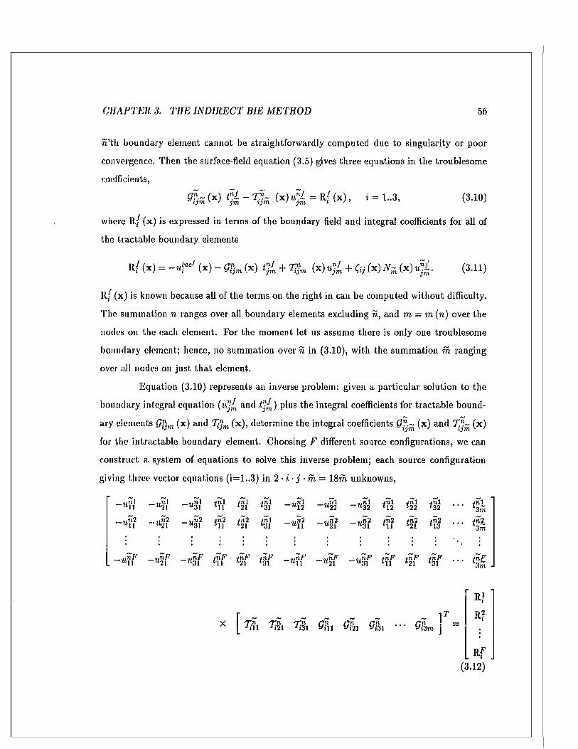
C H A P T E R 3. TH E IN D IR E C T BIE M E TH O D 56
n 'th boundary element cannot be straightforw ardly com puted due to singularity or poor
convergence. Then the surface-field equation (3.5) gives three equations in the troublesome
coefficients,
g f . ~ (x) C .L - (x) u ”l = R;? ( x ) , i = 1..3, (3.10)!jm ' > jm t jm ' ' jm 1 ' ' 1 ’ ' '
where ll/ (x) is expressed in term s of the boundary field and integral coefficients for all of
the tractable boundary elements
l l / (x ) = - u r / ( x ) - ^ m(x) t% + T*m ( x ) < + fo fx )^ V ~ (x)u g . (3.11)
B/(x) is known because all of the term s on the right in can be com puted w ithout difficulty.
The summation n ranges over all boundary elements excluding n, and m — m ( n ) over the
nodes on the each element. For the mom ent let us assume there is only one troublesome
boundary element; hence, no sum m ation over n in (3.10), with the sum m ation m ranging
over all nodes on ju st th a t element.
Equation (3.10) represents an inverse problem: given a particu lar solution to the
boundary integral equation {u '- jn and t",{) plus the integral coefficients for trac tab le bound
ary elements Qf-m (x) and T$m (x), determ ine the integral coefficients t/!l~ (x) and TJ}~ (x)
for tiic intractable boundary element. Choosing F different source configurations, we can
construct a system of equations to solve this inverse problem; each source configuration
giving three vector equations (i=1..3) in 2 • i • j • m = 18m unknowns,
_,„nl'Ml “21 “ «31 n lynl‘21 4TL1‘31 -T $ __ i,,nl “22 fnlz12 4 T l \‘22 JTll‘32 3m
_,,,n2 'Ml ,.n2U21 4n221 ynl31 ~ UU _„n2U21 ~ u3l 4V.2‘21 /n2‘l3 . tn23m
... H / ''Ml - U ~ l F“21 - t i f fmF‘31 - vnFMl _„nF“21 <
4nF‘21 vnF‘31 i n F3m ■
Vh Vil efn <4. Gil ••• G i n
11?
R?
R f (3.12)
C H A P T E R 3. T H E IN D IR E C T B IE M ETH O D 57
A t least 6m different source configurations are required to determ ine the integral
coefficients for one boundary element. My own BIE program , which uses a nine-node
boundary element scheme, needs at least 6m = 6 X 9 = 54 different; source configurations
for each troublesom e boundary element. Notice th a t the free-field m atrix has 6m columns
rather th an 18m, because there are three different vectors for the. right-hand side *=!,..3
giving th ree corresponding solution vectors. The free-field matrix on the left in (3.12) must
only be decomposed once to com pute all three sets of unknown vectors.
3.5.1 Several troublesom e elem ents
W hen several boundary elements are troublesome for the same computation point,
the system of unknowns and equations can be extended to include a set of unknown co
efficients for each of them : simply let the repeated index n imply summation over all
troublesome elements in (3.10), and add a proportional num ber of source configurations to
determ ine all of the in tractab le coefficients simultaneously. It may look as though we could
carry on this way to indirectly com pute all of the integral coefficients for a boundary integral
equation w ithout ever integrating numerically. I tried this using scalar integral equations
for fluid media, bu t found th a t the likelihood of an unstable free-field m atrix increases as
the num ber of troublesom e elements increases, so much so tha t it was irreparably unsta
ble whenever an inversion for all coefficients was attem pted. As mentioned in C hapter I,
Niku and B rebbia [94] proposed a to tal inversion scheme for a generic BIE m ethod, and
they suspected th a t instability would be a problem, much as I found. The indirect method
apparently works best when only a few troublesome boundary elements are encountered.
In elastic wave scattering I find tha t as many as six troublesome elements can be
handled in one equation with confidence, bu t there is no well-defined limit. To minimize
the num ber of troublesom e elements due to singularities, it is best to choose, surface-field
com putation points away from the perim eter of the boundary elements so they are in contact
with ju s t one element. This is why I included the flexibility to locate com putation points
anywhere on the surface in Section (3.2.1), ra ther than always using the element nodes as
routinely done in the BIE method.
C H A P T E R 3. T H E IN D IR E C T BIE M E TH O D 58
3 .5 .2 T h e p a r t i c u l a r s o lu t io n s
Following Niku and B rebbia [94’, let us call the free fields u ”f , t^ / and u f lc/
for / = 1..F the particular solutions. I t is evident th a t m any particu lar solutions will be
required to com pute troublesome integral coefficients—at least six configurations for each
node on each troublesome boundary element. In my own program , each particular solution
is due to a single point source having a different location and excitation. There is no rule for
source placement, but I have achieved best results when the sources are evenly d istributed
in both the interior and exterior domains when possible. There is also no explicit rule
regarding source excitation. For homogeneous perspectives I have had the best results
using a point forces having random orientation and complex excitation. More will be said
about the location and excitation of the particular solutions for layered m edia in C hapter
7.
It is advisable to use more particular solutions than strictly required, fur it is
possible to unknowingly specify particular solutions th a t leave the free-field m atrix il'-
oonditioned. Once again the over determ ined m atrix system can be solved using least-
squares. The troublesome coefficients should always be verified using the consistency test
in Section (3.3), before they are used in the BIE m ethod to identify any problems.
3 .5 .3 T h e i m p o r t a n c e o f t h e r e s id u e t e r m
It may appear th a t the coefficient Qj for the surface field equation, whose operation
has so far been treated as simple scalar m ultiplication5, could also be included as p art of
the unknown integral coefficients in (3.10), by rolling it in w ith the unknown 7??~ ra ther
than with R{ as in (3.11). This would be an advantage when the com putation point x is
located a t an edge or corner of the inclusion boundary where Cij (x ) is not known. But
consistency tests with coefficients computed with Cjj (x) rolled into failed when x lay
in a solid. The reason for failure is not known. I would venture th a t im portan t inform ation
is provided by explicitly setting Qj (x ) = 2 in (3.11), for it informs the inversion m ethod
th a t x lies on the boundary and th a t the boundary is smooth there, whereas rolling it in to
5Scc Section ('2.4).
C H A P T E R 3. TH E IN D IR E C T BIE M ETH O D 59
7;^- reduces (3.10) for x on the boundary to the same form as tha t for x in the interior,IJTTlthereby erasing all distinction between the surface- and null-field equations so far as the
inversion is concerned.
3 .5 .4 N o n u n iq u e i n d i r e c t c o e f f ic ie n ts
Inverse problems are notorious for having nonunique solutions [2*1], so it is no
surprise th a t the free-field m atrix determ ining the troublesome coefficients may be ill con
ditioned. In th a t case, I find a practicable solution can still be com puted using singular
value decomposition, which allows us to suppress the non-unique unstable part of the so
lution (the null-field of the free-held m atrix) by zeroing the smallest singular values in the
decomposition [100].
Nonuniqueness is easily dem onstrated in the case of fluid media,. Recall from (2.8)
tha t the stress in fluid m edia is directly proportional to the pressure times the boundary
norm al vector, = - p ! ^ n j . This makes three consecutive traction columns in the free-
held m atrix linearly dependent for each node immersed in a fluid, which in turn makes
the free-held m atrix singular and the solution vector nonunique. Indeed, the troublesome
coefficients cannot be com puted by m atrix inversion unless all groups of three offending
columns are grouped into one, or unless singular value decomposition (SVI)) is used.
The inferred coefficients are nonunique in another way. Imagine deforming the
shape of a troublesome element slightly by stretching in outwards from the original inclusion
while keeping its perim eter and the rest of the boundary unchanged. (If the element has a
surface-field com putation point on it, then the deformed element must still pass smoothly
through it.) The indirect method takes no account of such a deformation, neither in the
free-field m atrix (3.12) or the tractable integration term (3.11), so the same coefficients
would be inferred despite the deform ation, In a direct integration scheme, however, the
deformation would alter the coefficients for the element since they depend explicitly on its
shape.
The solution may be nonuniquo in other ways, but the question will not be pursued
further here. In practice we need coefficients tha t work in the boundary integral equation,
W hether the m ethod yields the same coefficients as direct integration, when tha t is possible,
C H A P T E R 3. T H E IN D IR E C T B IE M E T H O D 60
is a secondary question.
3.6 U sing H u ygen s’ principle to te st th e en tire BIE m ethod:
th e free-field test
An ingenious comprehensive test of the BIE m ethod was proposed by Schenck for
the Neumann problem for acoustics [106] [73]. We can apply it to elastic scattering as well
in the following way.
In the consistency test of Section (3.3), a subdomain of the original scattering
problem was embedded into a test problem in which it produced no scattered field so the
field a t the boundary nodes for a given source configuration could be com puted using only
the G reen’s function for the sources. R ather than assigning the complete field to each node
on the boundary to test the equation, let us now assign only p art of the boundary field to
each node using the boundary condition equations—either the displacement or traction—
and ask the BIE m ethod to com pute the unassigned part. How well the BIE m ethod
reproduces the unassigned p art of the field shows how well the m ethod can be expected to
perform in a particular application. The to tal coefficient m atrix for the free-field test for
one perspective would be
B I S r yincb
BC ■ C
with m atrix partitions defined as in (3.9), and C holding the assigned free-field variables.
The B I S partition is the same as the one used for th a t perspective in the final scattering
problem, so the test includes the boundary element configuration, frequency and m edia of
the scattering problem at hand. I t also exercises all of the routines needed to numerically
com pute the boundary field. Active boundary conditions are rarely used in geoacoustics,
but it is always advisable to make provisions for them , if only to perform this conclusive
test.
We can also test the next step in the BIE m ethod, by com puting the displacement
a t any point x in the interior domain to verify the accuracy of the whole field equation
(3.7). Usually the results of the second step are more accurate than the first because the
C H A P T E R 3. T H E IN D IR E C T BIE M ETH O D ()1
whole-field equation tends to average over numerical errors in the boundary field.
3.7 T esting th e boundary field: th e null-field test
Once the boundary field for an actual scattering problem has been computed, it
can be tested using the null-field equation, simply by checking th a t the newly computed
boundary field gives the null result a t points x in the exterior domain of the perspective
[114][73]. A boundary field th a t does not satisfy the null-field equation this way must be in
error, possibly because some integral equation coefficients were inaccurately com puted, the
field was inadequately sampled by nodes on the boundaries, or the total coefficient m atrix
suffered from instability. Exact zero is unlikely because numerical com putations are always
subject to some degree of error, so we need a measure against which the integral must
appear negligibly small. One measure could be taken from the incident field, |u m,’ (x ) |,°
provided x was no t close to a null in the incident displacement field. A better measure is
to use the m axim um displacement on the boundary m a x |u m| , which is independent of x.
3.8 M easuring error in num erical tests
W hen verifying the BIE m ethod in a test, whether in the free-field test or a, bench
mark scattering problem solved by different means, it is difficult to measure the error :n the
field using a single quantity. We could measure error in the displacement field relatively as
doing the same for traction, bu t this can make the error look deceptively small when there
are large | u CXa c t | a t ju st relatively few points. Nevertheless, it often works well for low
frequency scattering problems, when the wavelength is larger than the dimensions of the
scattering object, because the m agnitude of the exact field is not likely to vary dram atically
over its boundary. One alternative is to use a weighted average in place of the maximum
norm
erri (x ) = 100% X | Mnuinerical (x ) ~ U<;xact (x )|max |u„Xact |
(3.14)
err2 (x ) = 100% X (3.15)
6 |u | = s ju k u ‘k) where * denotes complex conjugate.
C H A P T E R 3. T H E IN D IR E C T B IE M ETH O D 62
but this can make the error look deceptively large when the field over p art of the boundary is
identically zero due to the boundary conditions. If p art of the boundary to a solid inclusion
is im penetrably rigid, for example, the average of |u exact| over the rigid p art will be zero,
reducing the overall average considerably, amplifying err2. A th ird m ethod is to use the
exact field at the point itself for the norm
err3 (x) = 100% X (x ) ~ ^ ct (x)||u eXact(x)|
but this obviously suffers when the field at x is very small, for it ranks the errors over parts
of the boundary th a t contribute very little to the boundary integral equal (where u is small)
with those tha t contribute significantly.
As I will only be considering low to mid frequency scattering problems, I will
report errors in the boundary field using (3.14), and include the ratio
err2 (x ) / enq (x ) = m ax |u exact| / avg |u cxact| , (3.17)
which converts e r q to enq . For points ofF all boundaries, however, I will use err3 (x ) because
I Ucxiict (x ) | removes the effect of decay with distance.
3.9 Exam ple: P lan e w ave scattering by spheres
To dem onstrate the indirect BIE m ethod, I will apply it to the scattering of plane
waves by rigid, fluid and solid spheres embedded in unbounded homogeneous domains for
which analytic solutions, by separation of variables, are available.7 The following variables
7Thc analytic solutions are of course evaluated numerically, and this is no easy task. T heir numerical representations often cannot be com puted for all ranges, directly on the boundary of the scattering sphere for instance, because terms in their series representation or the series itself becomes in tractable, I was unable to com pute the field on the boundary of the scattering spheres, for example, so the comparisons of the boundary field could not be made.
C H A P T E R 3. T H E IN D IR E C T B IE M ETH O D 63
are used throughout this section:
n
a
&o,Po,Po
a i ,P u P i
€
radius of spherical boundary,
elastic param eters outside sphere,
elastic param eters inside sphere,
P wavenumber outside sphere = 27r//«o,
P wavelength outside sphere = 2ic/kao,
kaQ Cl,close neighborhood of com putation point
within which a boundary element is doe mod troublesome,
boundary unit norm al vector,
Vi,V2, n = three m utually perpendicular unit vectors.
There are at m ost two perspectives for the boundary integral equations: perspective 0 is
the unbounded homogeneous domain outside the scattering sphere, and perspective I the
finite domain inside, when the sphere is penetrable.
3.9.1 Plane wave scattering from a rigid sphere in a fluid
The BIE m ethod will be verified .. »wo ways for an unbounded fluid domain; using
1) the free-field test, and 2) the analytic solution to the scattering of a plane wave by a rigid
sphere immersed in a fluid [91]. T he boundary elements and nodes comprising the sphere are
shown in Fig. (3.2). A to ta l of 366 particular solutions were used to determ ine troublesome
integral coefficients (150 randomly distributed inside, 216 on rectangular grid length On, on
a side, with no source closer than e = 0.2a to the boundary), each being generated by a
point force with a random ly assigned direction. One set of troublesome coefficients arose for
each boundary element in contact with the com putation point generating each surface-field
equation due to singularity. Details of the BIE set up are tabulated in 'fab le (3.1).
Free-field test
Recall th a t the spherical inclusion is not rigid in the free-field st, hi t is filled
with the same medium as the host domain to preclude scattering. Nevertheless, the same
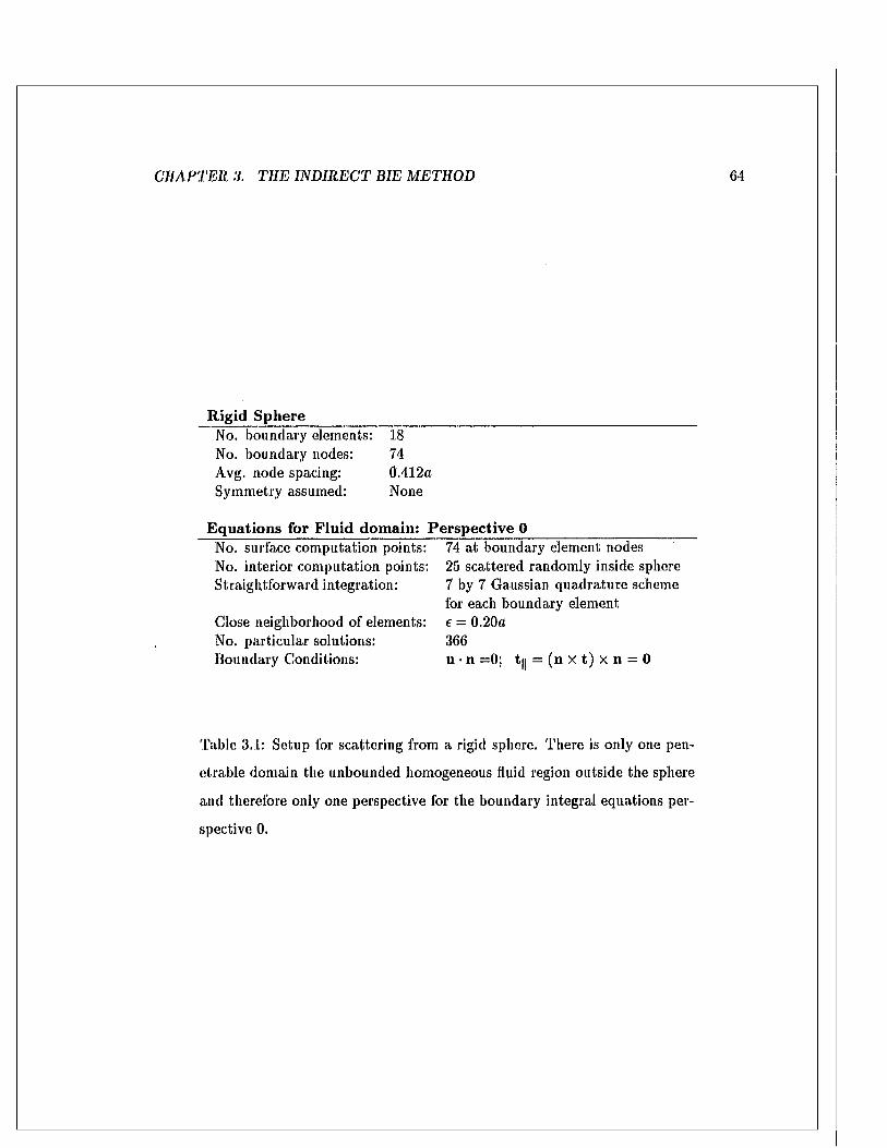
C H A P T E R 3. T H E IN D IR E C T BIE M E TH O D 64
Rigid Sphere_________No. boundary elements: 18No. boundary nodes: 74Avg. node spacing: 0.412aSymmetry assumed: None
Equations for Fluid domain: Perspective 0No. surface com putation points: No. interior com putation points: Straightforw ard integration:
Close neighborhood of elements: No. particu lar solutions: Boundary Conditions:
74 at boundary element nodes 25 scattered random ly inside sphere 7 by 7 Gaussian quadratu re scheme for each boundary element e = 0.20a 366u • n =0; t|| = (n X t) X n = 0
Table 3.1: Setup for scattering from a rigid sphere. There is only one pen
etrable domain the unbounded homogeneous fluid region outside the sphere
and therefore only one perspective for the boundary integral equations per
spective 0.
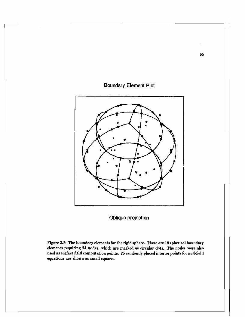
65
Boundary Element Plot
Oblique projection
Figure 3.2: The boundary elements for the rigid sphere. There are 18 spherical boundary elements requiring 74 nodes, which are marked as circular dots. The nodes were also used as surface field computation points. 25 randomly placed interior points for null-field equations are shown as small squares.
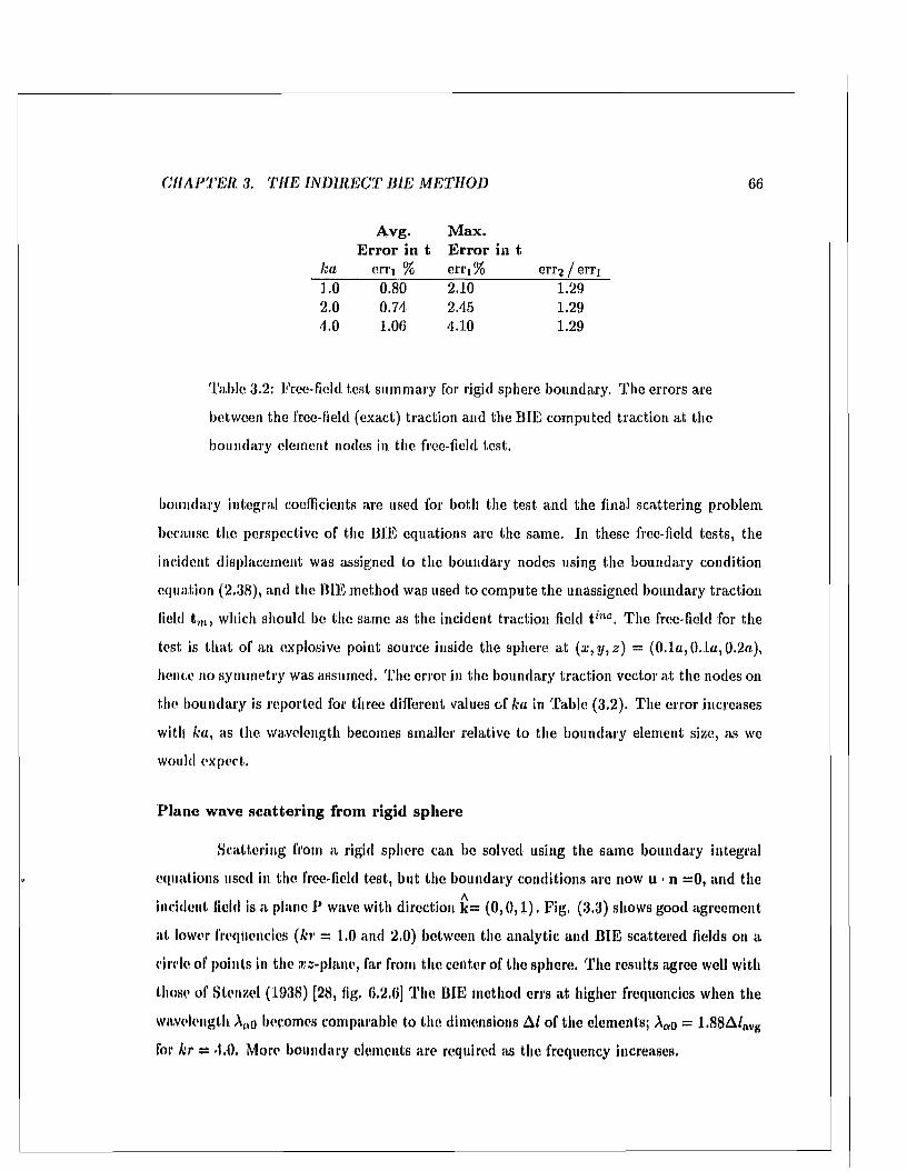
CHAPTER. 3. T H E IN D IR E C T BIE M ETH O D 66
Avg. Max.Error in t Error in t
ka erri % erti%_______ eiT2 / erri1.0 0.80 2.10 1.292.0 0.74 2.45 1.294,0 1.06 4.10 1.29
Table 3.2: 'Free-field test sum m ary for rigid sphere boundary. T he errors are
between the free-field (exact) traction and the BIE com puted traction a t the
boundary element nodes in the free-field test.
boundary integral coefficients are used for both the test and the final scattering problem
because the perspective of the BIE equations are the same. In these free-field tests, the
incident displacement was assigned to the boundary nodes using the boundary condition
equation (2.38), and the BIE m ethod was used to compute the unassigned boundary traction
field tm, which should be the same as the incident traction field t,nc. The free-field for the
test is th a t of an explosive point source inside the sphere a t ( x , y , z ) = (0.1a, 0.1a, 0.2a),
hence no sym m etry was assumed. T he error in the boundary traction vector a t the nodes on
the boundary is reported for three different values of ka in Table (3.2). The error increases
with ka, as the wavelength becomes smaller relative to the boundary element size, as we
would expect.
Plane wave scattering from rigid sphere
Scattering from a rigid sphere can be solved using the same boundary integral
equations used in the. free-field test, but the boundary conditions are now u • n =0, and the
incident field is a plane P wave with direction k= (0 ,0 ,1 ) . Fig. (3.3) shows good agreem ent
a t lower frequencies (hr — 1.0 and 2.0) between the analytic and B IE scattered fields on a
circle o f points in the ais-plane, far from the center of the sphere. T he results agree well with
those of Stenzel (1938) [28, fig. 6.2.6] T he BIE m ethod errs a t higher frequencies when the
wavelength A(,o becomes comparable to the dimensions A / of the elements; Aao = 1.88A/avg
for kr = <1.0. More boundary elements are required as the frequency increases.
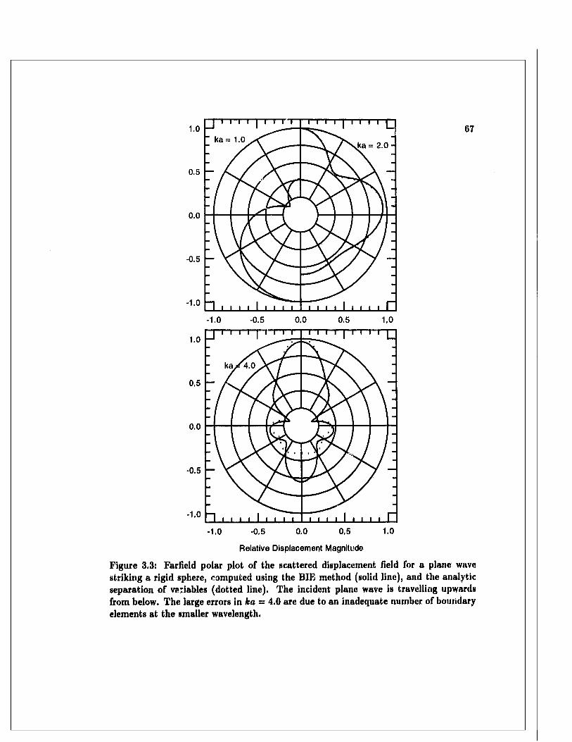
j i i i i | i i n
k a = 1.0
l l l l I I l I I |_
ka = 2 .0 -
67
~ i i i i i i i i i i i i i i i i i i i r ~-1.0 -0.5 0,0 0.5 1,0
"1 ,° l ~ i 1 1 1 1 1 1 1 t ~i I r T 1 1 1 1 1 1 1 r
-1,0 -0.5 0.0 0.5 1.0
Relative Displacement Magnitude
Figure 3.3: Farfield polar plot of the scattered displacement field for a plane wave striking a rigid sphere, computed using the BIE method (solid line), and the analytic separation of variables (dotted line). The incident plane wave is travelling upwards from below. The large errors in ka = 4.0 are due to an inadequate number of boundary elements at the smaller wavelength.
C H A P T E R 3. T H E IN D IR E C T B IE M E TH O D 68
3.9.2 Fluid sphere in a fluid
Here the BIE m ethod is verified for the scattering of a plane waves by a penetrable
fluid sphere immersed in an unbounded homogeneous fluid domain. T he fluid has an unre
alistic phase speed ( a = 6000 m /s) to correspond as much as possible to the solid sphere
considered later. The boundary elements and nodes comprising the sphere are shown in
Fig.(O/l), and the numerical param eters are tabulated in Table (3.3). In this case bilateral
symmetry about the plane y = 0 was used to reduce the num ber of unknowns by roughly
one half, The boundary and continuity conditions are the slip conditions for penetrable
fluid boundaries from Section (2.3.2). Fig. (3.5) shows good agreem ent in the far-held
polar plot of the scattered field using an analytic separation of variables m ethod and the
BIE m ethod.8 A = 2 .I7A /avg and 1.63 A/,lvg for perspectives 0 and 1, respectively, when
hr = '1.0.
3.9.3 Solid sphere in a solid
Here the BIE method is applied to scattering of a plane waves by a penetrable
solid sphere immersed in an unbounded homogeneous solid domain. The boundary elements
and nodes comprising the sphere are the same as in Fig.(3.4); the particulars are tabulated
in 'fable (3.4). Bilateral symmetry about the plane y - 0 was used again to reduce the
number of unknowns. The boundary and continuity conditions are those, for penetrable
solid boundaries in welded contact from Section (2.3.1). Fig. (3.6) shows good agreem ent
in the lar-field polar plot of the scattered field using an analytic separation of variables
method and the BIE method, These results duplicate those of Korneev and Johnson [75].
Fig. (3.7) shows a grey-scale plot of the total field in the exterior domain. The field is dark
in the interior of the sphere because the exterior perspective was used at every point in
plot; points inside the sphere being mill-field points where the boundary integral m ust give
zero. The boundary field therefore passes the null-field test of Section (3.7), To view the
field inside the sphere we m ust reverse the perspective as shown in Fig. (3.8).
"l am indebted to Dr. Trevor Dawson who provided the main subroutines for evaluating the scattered field using a separation of variables method [75] for the penetrable fluid and solid spheres.
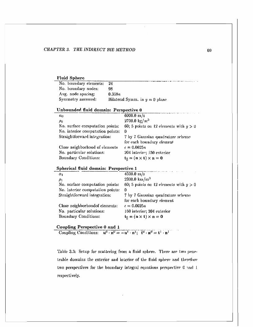
C H A P T E R 3. TH E IN D IR E C T B IE M ETH O D 69
Fluid SphereNo. boundary elements: 24 No. boundary nodes: 98 Avg. node spacing: 0.358aSymmetry assumed: B ilateral Symm. in y — 0 plane
Unbounded fluid domain: Perspective 0a 0 6000,0 m /s po 2700.0 leg/m3No. surface com putation points: 60; 5 points on 1,2 elements with y > 0 No. interior com putation points: 0Straightforw ard integration: 7 by 7 Gaussian quadrature scheme
for each boundary clement Close neighborhood of elements c = 0,0625a No. particular solutions: 204 interim'; 150 exterior Boundary Conditions: t|| = (n x t) X n = 0
Spherical fluid domain: Perspective 1« i 4500.0 m /spi 2300.0 km /m 3No, surface com putation points: 60; 5 points on 1.2 elements with y > 0No. interior com putation points: 0Straightforw ard integration: 7 by 7 Gaussian quadrature scheme
for each boundary element Close neighborhoodof elements: c = 0.0625a No. particular solutions: 150 interior; 204 exterior Boundary Conditions: ty = (n X t) x n = 0
Coupling Perspective 0 and 1Coupling Conditions: u{J ■ n° = - u 1 • n‘; tu - n° = t ' ■ n1
Table 3.3: Setup for scattering from a fluid sphere. There are two pene
trable domains the exterior and interior of the fluid sphere and therefore
two perspectives for the boundary Integral equations perspective 0 arid. 1
respectively.
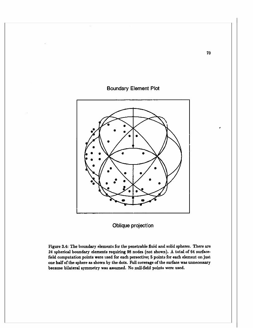
70
Boundary Element Plot
Oblique projection
Figure 3.4: The boundary elements for the penetrable fluid and solid spheres. There are 24 spherical boundary elements requiring 98 nodes (not shown). A total of 64 surface- fleld computation points were used for each persective; 5 points for each element on just one half of the sphere as shown by the dots. Full coverage of the surface was unnecessary because bilateral symmetry was assumed. No null-field points were used.
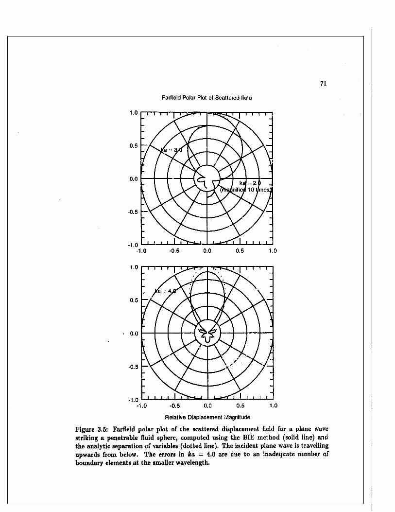
71
FarfieSd Polar Plot of Scattered field
T T I I I I
Relative Displacement Magnitude
Figure 3.5: Farfield polar plot of the scattered displacement field for a plane wave striking a penetrable fluid sphere, computed using the BIB method (solid line) and the analytic separation of variables (dotted line). The incident plane wave is travelling upwards from below. The errors in ka = 4.0 are due to an inadequate number of boundary elements at the smaller wavelength.
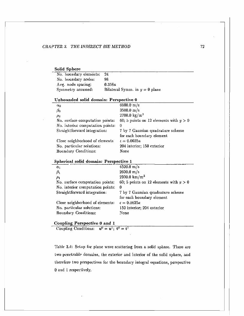
CHAPTER. 3. T H E IN D IR E C T BIE M E TH O D 72
Solid SphereNo. boundary elements: 24No. boundary nodes: 98Avg. node spacing: 0.358aSymmetry assumed: B ilateral Symm. in y = 0 plane
U nbounded solid domain: P erspective 0a 0 6000.0 m /sfto 3500.0 m /sPi) 2700.0 kg/m 3No. surface com putation points: 60; 5 points on 12 elements with y > 0No. interior com putation points: 0Straightforw ard integration: 7 by 7 Gaussian quadrature scheme
for each boundary elementClose neighborhood of elements £ = 0.0625aNo. particu lar solutions: 204 interior; 150 exteriorBoundary Conditions: None
Spherical solid domain: P erspective 14500.0 m /s
Pi 2600.0 m /sPi 2300.0 km /m 3No. surface com putation points: 60; 5 points on 12 elements with y > 0No. interior com putation points: 0Straightforward integration: 7 by 7 Gaussian quadratu re scheme
for each boundary elementClose neighborhood of elements: e = 0.0625aNo. particular solutions: 150 interior; 204 exteriorBoundary Conditions: None
Coupling P erspective 0 and 1Coupling Conditions: u° = u1; t° = t ]
Table 3.4: Setup for plane wave scattering from a solid sphere. There are
two penetrable domains, the exterior and interior of the solid sphere, and
therefore two perspectives for the boundary integral equations, perspective
0 and 1 respectively.
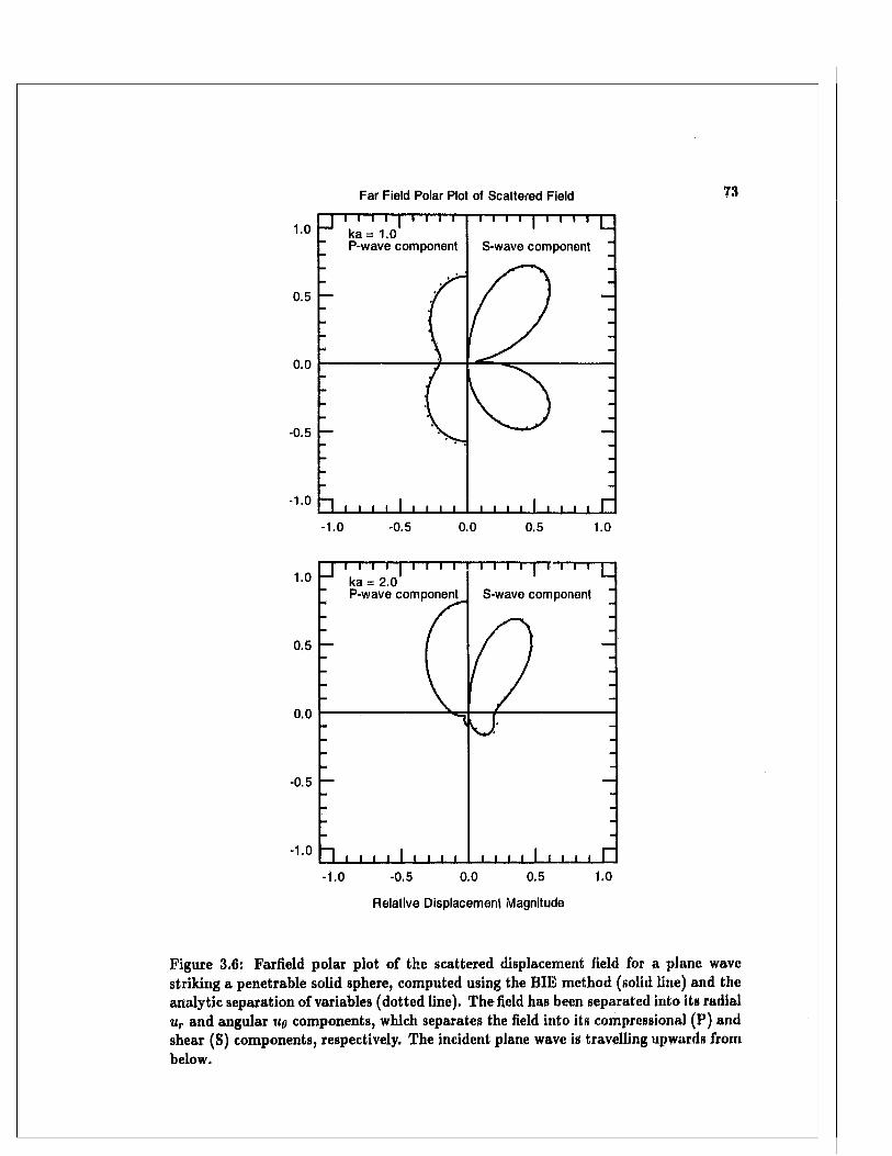
Far Field Polar Plot of Scattered Field
ka = 1.0P-wave component S-wave component
0.5
0.0
-0.5
- 1.0
-1.0 -0.5 0.0 0.5 1.0
ka = 2.0P-wave component S-wave component
0.5
0.0
-0.5
-1.0 -0.5 0.0 0.5 1.0
Relative Displacement Magnitude
Figure 3.6: Farfield polar plot of the scattered displacement field for a plane wave striking a penetrable solid sphere, computed using the BIE method (solid line) and the analytic separation of variables (dotted line). The field has been separated into its radial ur and angular uq components, which separates the field into its compressional (F) and shear (S) components, respectively. The incident plane wave is travelling upwards from below.
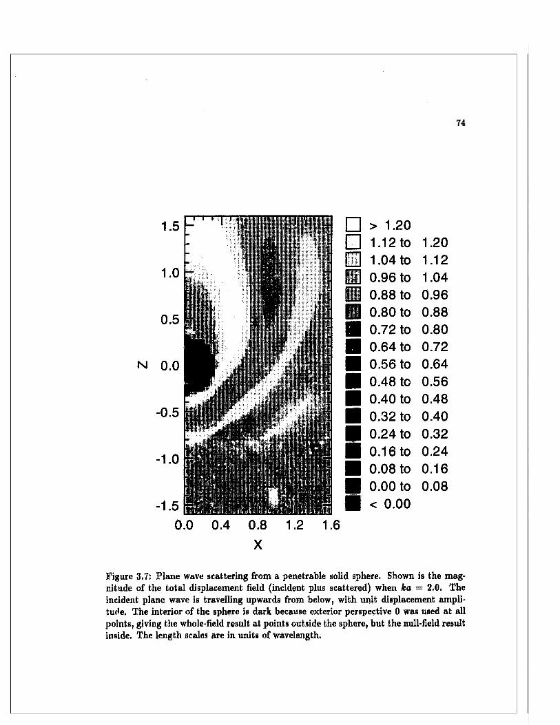
74
N
5* 'i w w nssKmjfSi
-0.5
> 1.20 1.12 to 1.04 to 0.96 to 0.88 to 0.80 to 0.72 to 0.64 to 0.56 to 0.48 to 0.40 to 0.32 to 0.24 to 0.16 to 0.08 to 0.00 to < 0.00
1.201.121.040.960.880.800.720.640.560.480.400.320.240.160.08
0.0 0.4 0.8X
Figure 3.7: Plane wave scattering from a penetrable solid sphere. Shown is the magnitude of the total displacement field (incident plus scattered) when ka = 2.0. The incident plane wave is travelling upwards from below, with unit displacement amplitude, The interior of the sphere is dark because exterior perspective 0 was used at all points, giving the whole-field result at points outside the sphere, but the null-field result inside. The length scales are in units of wavelength.
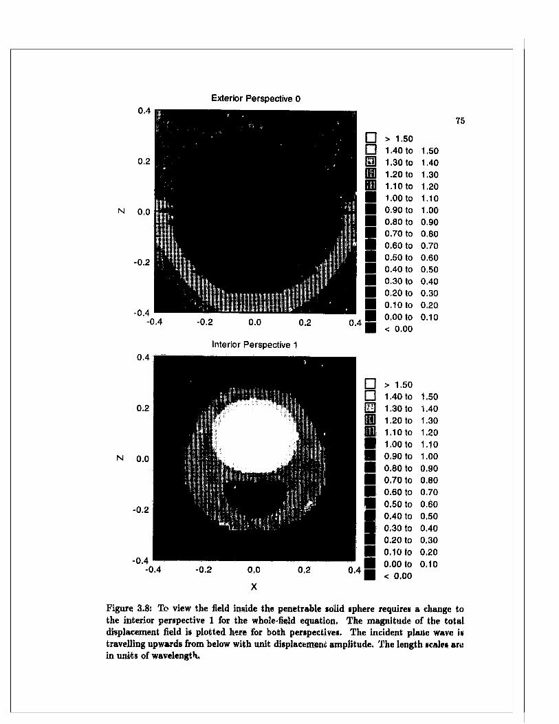
Exterior Perspective 0
N o.O
N 0 .0
- 0.2
-0.4
Interior Perspective 1
□ > 1.50□ 1.40 to 1.50B 1.30 to 1.40n 1.20 to 1.30■ 1.10 to 1.20■ 1.00 to 1.10■ 0.90 to 1.00■ 0.80 to 0.90■ 0.70 to 0.801 0.60 to 0.70■ 0.50 to 0.60■ 0.40 to 0.50■ 0.30 to 0.40■ 0.20 to 0.30■ 0.10 to 0.20■ 0.00 to 0.10■ < 0.00
V
□ > 1.50□ 1.40 to 1.50n 1.30 to 1.40H 1.20 to 1.30■ 1.10 to 1,20■ 1.00 to 1.10■ 0,90 to 1.00■ 0.80 to 0.90■ 0.70 to 0,80■ 0.60 to 0.70■ 0.50 to 0.60
■ 0,40 to 0.50
I 0,30 to 0.40■ 0.20 to 0.30■ 0,10 to 0.20■ 0.00 to 0.10■ < 0,00
75
Figure 3.8: To view the field inside the penetrable solid sphere requires a change to the interior perspective 1 for the whole-held equation. The magnitude of the total displacement field is plotted here for both perspectives. The incident plane wave is travelling upwards from below with unit displacement amplitude. The length scales are in units of wavelength.
76
C h a p t e r 4
The field from a point source in
layered m edia
T he BIE m ethod requires a G reen’s function for each perspective in the scattering
problem. The Green’s function for an unbounded homogeneous medium can be w ritten in
closed form and is easily com puted, whereas the G reen’s function for layered m edia m ust
be w ritten in terms of integral transform s th a t are much more difficult to evaluate. The
numerical methods for layered m edia have improved considerably since Thom son [124] and
Haskell [56] first formulated their propagator m atrix approach, bu t the essentials remain the
same: Fourier-Bessel integral transform s separate the vertical and horizontal dependence of
the field reducing the problem to two independent boundary value problems in the vertical
dimension alone; one for coupled shear and compressional wave m otion (P-SV) and another
for strictly shear (SH), These are solved numerically using m atrix m ethods.
In this chapter I review the m atrix m ethod for layered m edia and make a few
contributions of my own. In particular, using a numerically stable scattering matrix m ethod,
I show how the wave field can be illustrated using a schematic “ladder” diagram like the
diagrams engineers might use to analyze linear systems, which is helpful for illustrating the
operation of m atrix m ethods for layered media. I rely heavily on K ennett’s m onograph on
seismic waves [71] throughout this chapter, following his m ethod and notation as much as
possible, and adding results for fluid layers as required, T he extension from an integral

C H A P T E R 4. T H E FIELD F R O M A PO INT SOURCE IN L A Y E R E D MEDIA 77
transform to a norm al m ode representation of the Green’s function is taken up in the next
chapter. It should be emphasized th a t here we are concerned with computing the G reen’s
function in the absence of scattering objects. We shall re turn to scattering in layered media
using the BIE m ethod in C hapter 7.
4.1 The tw o-point boundary value problem
Using a cylindrical polar coordinate system (»•,«£,z), in which the cr-axis points
vertically downwards, the displacement field, the equation of motion (2. Id), and Hooke’s
law (2 .2) become
u (r, </>, z, t) = u r(r, </;, z, t) e r + u ^ r , </>, z, I) e 4, -f- uz{r, </>, z , /) e 2 , (d . I )
pdUUr = OzTrz + 0 TTrr + r ~ ld + T~l ( rn . + Pfr
p d u H = OzTfa + dr Tr,l> + r~ l d , j , T + 2r~ 1 Tri + p U
pduUz = 0ZTZZ -f- drTrz + r _ lc),/,r,/)2 + r ~ l rrz + Pfz
Trr - (A + 2u) drur -|- A {dzuz + r ~ { (Ofu,j, -j- 'til•)} )
= (A + 2/r) + ur ) + A {0zuz + Or'tl'i0 ,
Tzz = (A -f 2/i) dzu , + A {dru r + r ~ l (0,y«,/, + n ,•)}Trz = p, (dzur + druz ) ,
Tij>z — P (,1‘ -f" dz'tli/,) ,
7~Ttfi ~ f t (Op "f" 7* drfi'llp V »
e r ,e 0 and e- are the unit vectors of the coordinate system, and f = [ / r ,/,/»./*]1 in the
body force. Since the displacement and the traction m ust be continuous across an interface
between layers, wo might expect th a t u , and traction vector acting on a horizontal surface
element
t( r , (p, z, t) = Trz(r, <l>, z . /,) e r + r,/,2(r , <j>, z, I,) e,/, + rzz{i\ </>, z, I) e , , (4 A)
should play an im portan t role, whereas the remaining three elements of stress, r r r ,r,/„/, and
rr4> m ight be elim inated, In fact, it can be shown [.'55] th a t (4.2) and (4,3) reduce to two
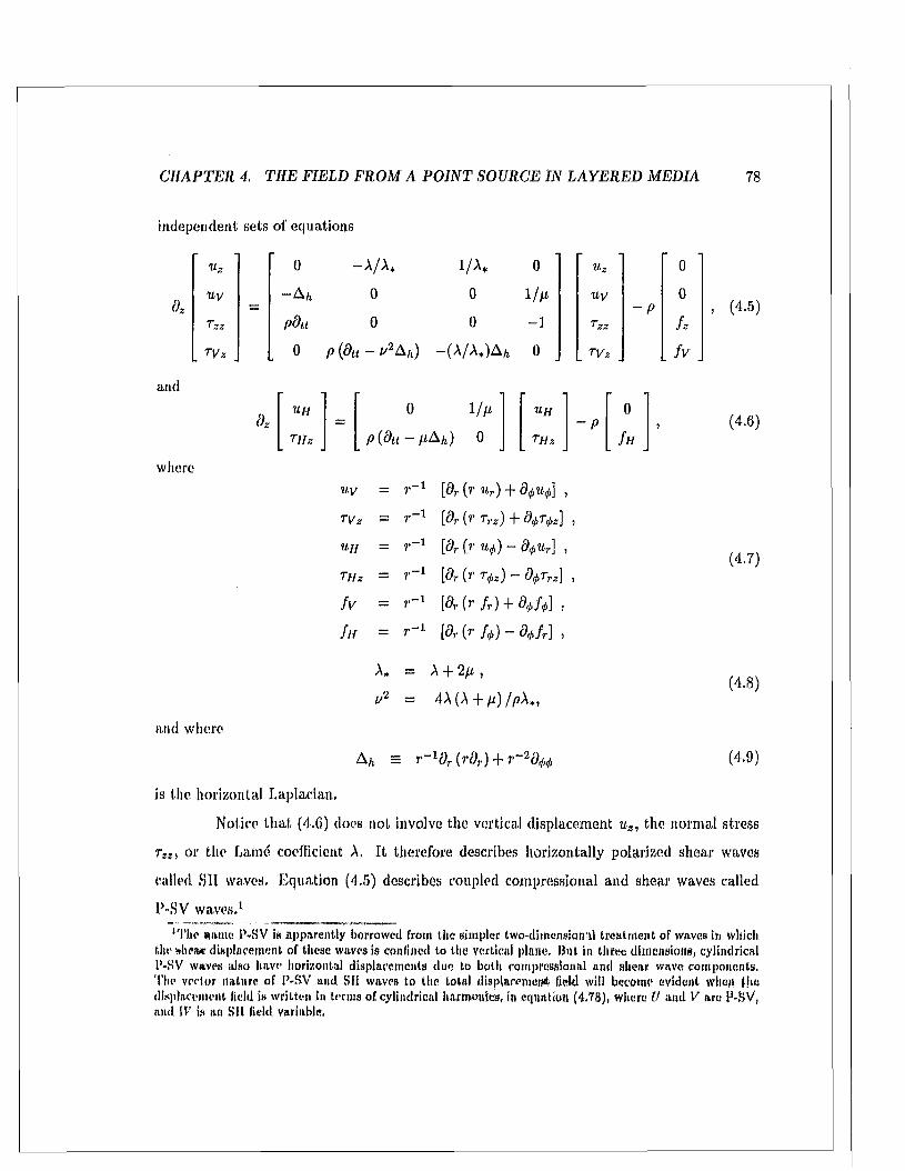
C H A P T E R 4, T H E FIELD F R O M A P O I N T SOUR CE I N L A Y E R E D M E D IA 78
independent sets of equations
Uz
U y
7 zz
. TVz .
and
where
and where
0 - A / A , 1 /A
- A h 0 0
pda 0 0
0 p (dtt - v 2 A h) - ( A /A *
Oz
0 uz 0
1 I n u y 0- P
- 1 7'zz f z
0 . TVz . f v
Ufl _ 0 1 / n UH~ P
0
TJIz 1
I 'hi > o1 THz Sh
uy
rvz
Uf f
Tllz
f v
f ir
A* =
[dr (r Ur ) - f d j Uj , ] ,
[dr ( r Tr z ) + df iTfa]
[dr (»• H ) ~ d'f>Ur\ i
[dr (r rljlz) - d ^T r z] ,
[dr ( r f r ) + d + f a ] ,
[dr ( r U ) - d, j, fr] ,
A + 2 p, ,
4A (A + /i) / p \ * ,
(4-5)
(4.6)
(4.7)
(4.8)
(4,9)A h = r-H)T (rdr ) + r -* d H,
is the horizontal Lap! an an.
Notice th a t (4.6) does not involve the vertical displacement uz , the norm al stress
r 9z) or the Lame coefficient A. I t therefore describes horizontally polarized shear waves
called S ll waves. Equation (4.5) describes coupled compressional and shear waves called
P-SV waves,1
1 The name P-SV is apparently borrowed from the simpler two-dimensional trea tm en t of waves in which the shea* displacem ent of these waves is confined to the vertical plane. B ut in three dimensions, cylindrical P-SV waves also have horizontal displacements due to both compressional and shear wave components. The vector nature of P-SV and SJI waves to the total displacem ent field will become evident when the displacem ent field is w ritten in terms of cylindrical harmonies, in equation (4.78), where V and V are P-SV, and IF is an S ll field variable.
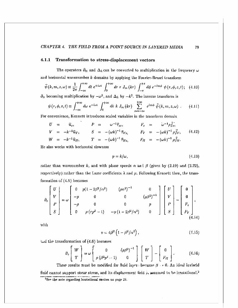
C H A P T E R 4. T H E FIELD F R O M A P O IN T SOURCE IN L A Y E R E D MEDIA 79
4.1.1 Transformation to stress-displacem ent vectors
The operators d t t and A/t can be converted to m ultiplication in the frequency u>
and horizontal wavenumber k domains by applying the Fourier-Bessel transform
- 1 f+°° , • . f+°° r+n ■ ,■$(k ,m , z ,u j )= — dt e+lwt dr r Jm (kr) J d<j> e (1.10)
d tt becoming m ultiplication by - u j 2 , and A/, by - k 2 . The inverse transform is
/ -foo Z+CO ^*°° ^du e~lwl / dk k Jm (At) J ] V>(k , m , z , u ) . (4.11)
•°° Jo m = -o o
For convenience, K ennett introduces scaled variables in the transform domain
u = u z , P = w l Tz z , Fz = w“ V /s i
V = - k ~ xu v , S - - (u k r 1 t v z , II 1 e' "'"'I (4.12)
w = - k r l u H, T = - (or/!)-1 T[[Z, /')/ = - M r v / , , .He also works w ith horizontal slowness
p = k / u ,
rather th an wavenumber k, and with phase speeds a an:l ji (given by (2.19) and (2,22),
respectively) ra ther than the Lame coefficients X and /t, Following K ennett then, the trans-
formation of (4.5) becomes
’ u 0 p (l -2 /4 2/ o 2) (pa2 ) - 1 0
V= UJ
- p o 0 (p/P)
p - p 0 0 P
. s . 0 P ( r p 2 ~ 1) - p (1 - ‘I / P / n 2 ) 0
-IU
V
P
s
0
0
/'»
Fv(‘ .14)
with
v ~ ~ 4 l P ( l ~ f i 2 / a i ) , (1.15)
and tilt* transform ation of (4.0) becomes
’ w] r 0 (PUT1] \ w" [ o 'd~ = o ) - : . (4.1(1)
T [P {ftV - i) 0 J [ T \ F,i JThese results m ust be modified for fluid layer - because /) * f). An ideal invisdd
fluid cannot support shear stress, and its displacement field is assum ed to he irrotatiorm l^
3See the note regarding irro tational rwotkni on page 24-
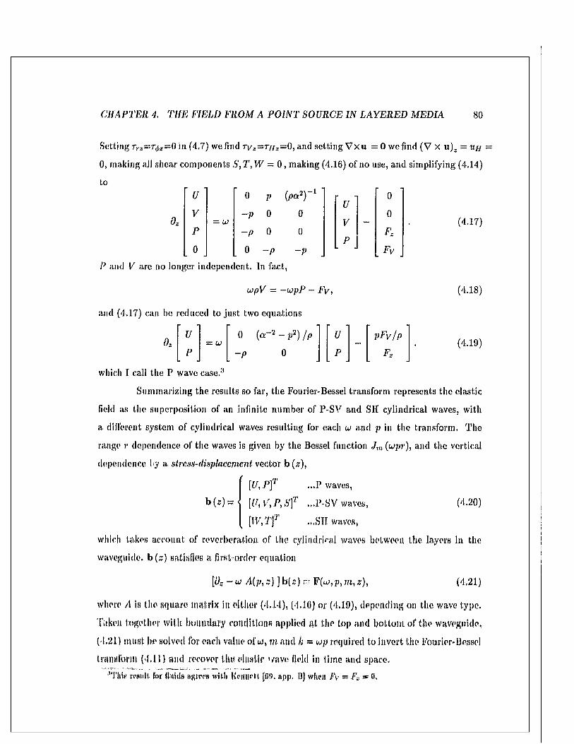
C H A P T E R 4. T H E FIELD F R O M A P O I N T SOUR CE I N L A Y E R E D MED IA 80
Setting Trz=T,i>z=0 in (4.7) we find t v z= tj[z=0, and setting V x u = 0 w efm d (V X u )2 = Ufj
0, making all shear components S, T, W = 0 , making (4.16) of no use, and simplifying (4.14)
to0 p (p a 2) -1
- p 0 0
- p 0 0
0 - p - p
P and V are no longer independent. In fact,
dz
’ u
V
p= u
0
_ 0u
0V
Fzp
L J. Fv .
(4.17)
u)pV = —u p P — F v ,
and (4.17) can be reduced to ju st two equations
U<h u>
ie*11oV pFv /p
- p 0 p Fz
(4,18)
(4.19)
which I call the P wave case.3
Summarizing the results so far, the Fourier-Bessel transform represents the elastic
field as the superposition of an infinite num ber of P-SV and SH cylindrical waves, with
a different system of cylindrical waves resulting for each u and p in the transform . The
range r dependence of the waves is given by the Bessel function Jin (upr), and the vertical
dependence by a strcsa-displaccrnent vector b (z),
b (* ) =
.P waves,
[U, V, P, S]r ...P-SV waves, (4.20)
. l » Y t f ...SH waves,
which takes account of reverberation of the cylindrical waves between the layers in the
waveguide, b (z) satisfies a first-order equation
[i)z - u ) A (p , s ) ]h[z ) c F(u;fj> ,m ,*), (4.21)
where A is the square m atrix in either (4.14), (4.10) or (4.19), depending on the wave type.
Tit ken together with boundary conditions applied a t the top and bottom of the waveguide,
(1.21) m ust b e solved for each value of u j , m and k = u p required to invert the Fourier-Bessel
transform (4.11) and recover the elastic wave field in time and space,
■'This result for fluids agrees with Kennett [00. app. I)) when Fv = F-. * 0.
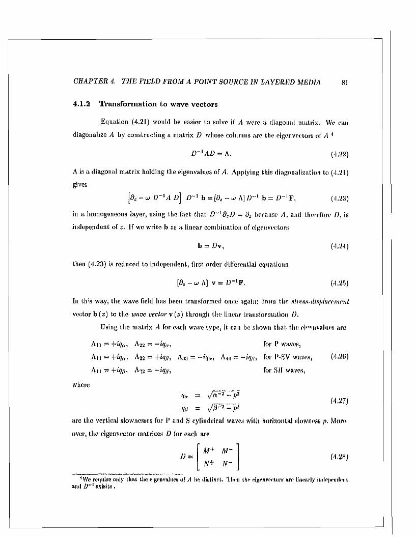
C H A P T E R 4. T H E FIELD F R O M A P O I N T SO URCE IN L A Y E R E D MEDIA 81
4.1.2 Transformation to wave vectors
Equation (4.21) would be easier to solve if A were a diagonal matrix. Wo can
diagonalize A by constructing a m atrix D whose columns are the eigenvectors of A *'
D ~ l A D = A. (.1.22)
A is a diagonal m atrix holding the eigenvalues of A, Applying this diagonalization to (4.21)
gives
[dz - u j D ~ l A D\ D ~ l b = [dz - w A ] D~' b = D ~ lF , (4.2:1)
in a homogeneous layer, using the fact tha t D ~ ldzD = i)z because A, and therefore D, is
independent of 0. If we write b as a linear combination of eigenvectors
b = D v , (4.24)
then (4.23) is reduced to independent, first order differential equations
[0Z - u> A] v = l )~ [F. (4.25)
In th ;s way, the wave field has been transformed once again: from the alrcHH-dispUimnenl
vector b ( z ) to the wave vector v ( z ) through the linear transform ation I).
Using the m atrix A for each wave type, it can be shown th a t the or'envalues are
A n = +i(ia, A22 = for P waves,
A n = +*</«, A22 = A33 = - i q m A,|,| = - i<ifi, for P-SV waves, (4.20)
A n - Ar)2 =• for Sll waves,
where
<h = - p2(4,27)
<H) ~ ~ Pl
arc the vertical slownesses for P and S cylindrical waves with horizontal slowness p. More
over, the eigenvector matrices I) for each are
M+ M w
N + N ~D (4.28)
1 We require only that the eificnvalues of A bn distinct. 'I fu n the eigenvectors arc linearly iwlc|>ciident and /2~l pxi»it» .

C H A P T E R 4. THE FIELD F R O M A P O I N T SO URCE IN L A Y E R E D MEDIA 82
with partitions
M ^ — h i f / a Ca
N *for P waves,
-P <0
M * =± i q a ea pep
pca ± i q p cp
p ( 2 f P p 2 - 1.) t« ± 2 i p / 3 2pqpCp
±2 ip f 32pqtl( a p (2f32p 2 - 1) ep
for P-SV waves (4,29)
M ± = cp/ji
N'h = ±ipftqpcpfor SH waves.
fn. and (p arc norm alization factors 0) applied to the columns of D. Any such norm al
ization can be used (because the columns of D, being eigenvectors of A, can be arbitrarily
scaled), but K ennett’s choice
Co, = (2pqu)~ x! 2 ,' (4.30)
(p = ( 2 w /? r l /2 ,
derived from vertical energy flow considerations,5 lias the advantage th a t D ~ l has the simple
form( N ~ f - ( M ~ f
- ( N + f (M + f
D~l is required later when considering the excitation due to a point source in Section
(4.2,5),
It is convenient to partition b into displacement w and stress t components,
b = [w, t ] 1 , such th a t (4.24) becomes
(4.32)
= i (4.31)
1
st— . 1
i* i
< +i
1 i
+ i
»
.............iI>
*
' Vit Ik i»l energy flow in cylindrical waves is considered la ter in Section (5.0),
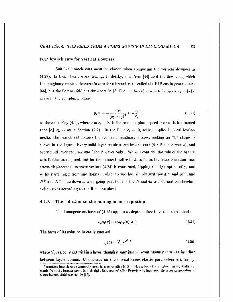
C H A P T E R 4. T H E FIELD F R O M A P O IN T SOURCE IN L A Y E R E D MEDIA S3
EJP branch cuts for vertical slow ness
Suitable branch cuts m ust be chosen when computing the vertical slowness in
(4.27). In their classic work, Ewing, Jarcletsky, and Press [44] used the line : 1 r; which
the im aginary vertical slowness is zero for a branch cut called the E JP cut in geoacoustics
[66], bu t the Soinmerfeld cut elsewhere [24].° The line !m {<■/} = </,■ = 0 follows a hyperbolic
curve in the complex p plane
'■“ ,1as shown in Fig. (4.1), where c = cr + i('i is the complex phase speed a or /I, ft is assumed
that |c/| < cr as in Section (2.2). In the limM —* 0, which applies in ideal lossless
media, the branch cut follows the real and imaginary p axes, making an “b” shape as
shown in the figure. Every solid layer requires two branch cuts (for P and S waves), and
every fluid layer requires one ( for P waves only). We will consider the role of the branch
cuts further as required, but for the m -menI, notice that, so far as the transform ation from
stress-displacernent to wave vectors (4.24) is concerned, flipping the sign option off/,, and
qp by switching p from one lliemann shorn. to another, simply switches A/+ and M" , and
N + and iV“ , The down and up going partitions of the D m atrix transformation therefore
switch roles according to the lliemann sheet.
4.1.3 The solution to the hom ogeneous equation
The homogeneous form of (4.25) applies at depths o ther than the source depth
Os'in(z) - ujXiVi(s) = 0. (4,34)
The form of its solution is easily guessed
V j ( z ) s V j r ^ 1*, (4.35)
where Y j Is a constant within a layer, though it m ay jum p discord!.: ' tom an interface
between layers because D depends on the discontinuous elastic param eters o r , /I and />,
“A nother branch cut commonly used in geoacoustics is the Pekeris branch cu t extending vertically up wards from the branch point in a straight line, named after Pekeris who first used them for propagation in a two-layered fluid waveguide [97].
94
125515
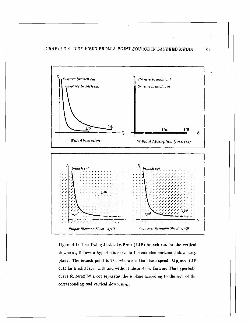
C H A P T E R 4. T H E FIELD F R O M A P O IN T SOURCE IN L A YE R E D MEDIA 84
P -w a ve branch cut
S -w ave branch cu t
1/a
With Absorpt ion
I)P -w ave branch cut
S -w ave branch cut
l/a 1/S^ l>
Without Absorpt ion (lossless)
branch cut
qr<0
Proper Riemann Sheet q >0
branch cut
Improper Riemann Sheet q .<0
Figure 4.1: T he Ewing-Jardet.sky-Press (E JP ) branch cut for the vertical
slowness q follows a hyperbolic curve in the complex horizontal slowness p
plane. T he branch point is 1 /c, where c is the phase speed. U p p e r : EJP
cut/: for a solid layer with and w ithout absorption, L ow er: The hyperbolic
curve followed by a cut separates the p plane according to the sign of the
corresponding real vertical slowness qr-
C H A P T E R 4. T H E FIELD F R O M A P O IN T SOURCE IN L A Y E R E D M ED IA 85
Substituting the eigenvalues (4.26) into (4.35) gives
VS(*) = Vi exp(±« u qa,p z), (4.36)
which is tlie vertical dependence of P and S cylindrical or plane waves in a homogeneous
medium. The vertical tw o-point boundary value problem would be solved if the complex
wave vector am plitudes where known at each interface in the waveguide. To com pute them
numerically we cast the vertical boundary value problem in m atrix form.
o u tpu t vector a t port A R AB rpAB input vector a t port A
o u tpu t vector a.t port B rpBA R BA input vector at port B
(4.38)
4.2 T h e scattering m atrix m ethod
A scattering m atrix is a transform ation from input variables to ou tpu t variables
for a linear network. If the inputs and outputs are accessed through two ports A and B as
shown in Fig. (4.2), the transform ation can be partitioned in this way
(4.37)
whereR A B = reflection m atrix seen at port A,
R B/1 = reflection m atrix seen at port B,
T a b = transm isison m atrix from port B to A,
T b a = transm isison m atrix from port A to B.
The m atrix partitions, represented using triangular symbols, act as m ultiplication operators
(or amplifiers) on the signals.
4.2.1 Scattering m atrix for a hom ogeneous layer
Let us form ulate the scattering m atrix for a homogeneous layer spanning the depth S
~A to zB \ z B > Zj\. T he inputs to the layer are the incoming wave vector elements, v+ (z a )
and v~ (zB ), and the ou tputs are the out going wave vector elements, v~ (z a ) and v+ (zB) ,
as shown in Fig.(4.3). T he scattering m atrix for a homogeneous layer is particularly simple
because transm ission through the homogeneous m edia is the same in both directions, and
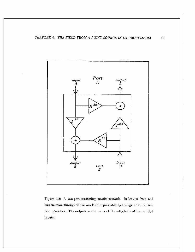
C H A P T E R 4. TH E FIELD F R O M A P O IN T SOURCE IN L A Y E R E D M ED IA 86
Portinput output
AB
ABBA
BA
inputou tpu tP ort
Figure 4.2: A tw o-port scattering m atrix network. Reflection from and
transm ission through the network are represented by triangular m ultiplica
tion operators. The outputs are the sum of the reflected and transm itted
inputs.

C H A P T E R 4. TH E FIELD F R O M A P O IN T SO URCE IN L A Y E R E D M E D IA 87
reflection from within the layer is zero. T he relation between inputs and outpu ts can be
written directly from (4.36) in m atrix form
V “ (z>i).
i-----
--< +
■
0 T l ( z b - * a )
T l I z b - Z a ) 0
where T b is the transm ission m atrix for the layer
eivqa(zB-ZA} 0T l (z b - z a ) = . ,
0 e1 W(ip(zb —*a )
T l ( z b - z a ) = eiwM * B -zA)
V + ( Zj l )
V~ (zB)= S
V + (zA)
V " ( z b )
...for P waves,
...for P-SV waves,
...for SH waves.
(4.39)
(4.40)
V e rtic a l e v a n e sc e n c e
In general the vertical slowness is complex, q — qT + *<?»> giving inhomogeneous
cylindrical wave behavior. The sign of </,- determines the vertical decay (or growth) of the
wave am plitude. W hen it is positive, the wave decays as it propagates, and we say th a t the
wave is vertically evanescent. W hen it is sufficiently large, the wave cannot traverse the
entire layer since ciwqh = e~UJ'l' k —► 0, cu tting off vertical transm ission through a, layer, in
effect separating the waveguide in two independent layer structures so far as th a t system of
cylindrical waves is concerned. Similar decoupling occurs through the accum ulated effect
of many th in consecutive evanescent layers.
4.2.2 Scattering m atrix for an interface between layers
T he coefficient m atrix A in (4.21) does not depend on the derivatives of the elastic
properties p ,a and /?, so the stress-displacem ent vector b for each wave type is continuous
a t an interface between layers on which there is no source (F — 0); th a t is,
b ( z f ) = b (* f ) ,
a t interface z( , where z f = Z[±. c, in the lim it e -» 0+ . This implies
D a v ( z j ) - D b v ( z f ) ,
(4.41)
(4.42)
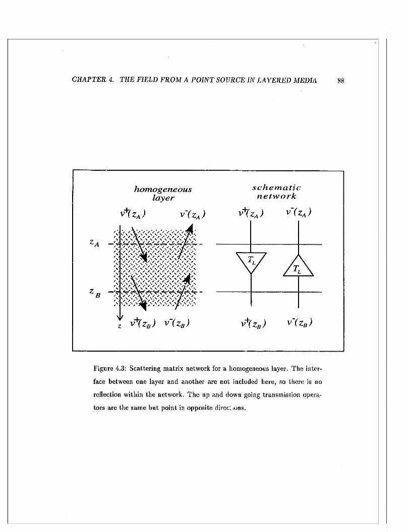
C H A P T E R 4. TH E FIELD F R O M A P O IN T SO URCE IN L A Y E R E D MEDIA 88
h o m o g e n e o u sl a y e r
V+( z A ) v ' ( z A ) v+(
f '* V / *V*x V V ' / V V V *V S S S f c S S \ S S \ N \ \ t - x x x \x x x x x x x x x x / x_ \ \ \ s \ \ S \ S S N \ N \ y \ N7 . ' - x x x Y x x x x x x x x x / x x
s c h e m a t i cn e t w o r k
zA ) v ( Z - J
** ' - x x x A x x x x x x x x / x x\ / S 'S S/ . y v ./ / v . y * s s s J *U y yS \ S \ \ A \1 V t 4 x x x x W x x x x x x - y x x x \ n
' - X X X X A x x x x x x x x x x \ i' - x x x x x x x x x x x x x x x \
x x x x x x x x x x x x x x x \/ < x x \ x x x x x x x x x x x b x' - X X ¥ x x x x x x x x x ^ T x \ \ \ s \ \ \ \ \ \ \ \ \ \ \ A \ f d / / A x x x x x x x x x x / x X \ 1
\n ' - x x x A x x x x / x x x / x x x
' - X X X X \X J x x x x x x Y x x x \ \ \ \ \ # f k N S S % S \ / \ S S S / . * t t y y y / y / J p / / /
Z v+( z D) v ~ ( z B ) v+( z j v’( Zn)
Figure 4.3: Scattering m atrix network for a homogeneous layer. The ‘ ‘ -
face between one layer and another are not included here, so there is no
reflection w ithin the network. T he up and down going transm ission opera
tors are the same but point in opposite direc', ions.
81
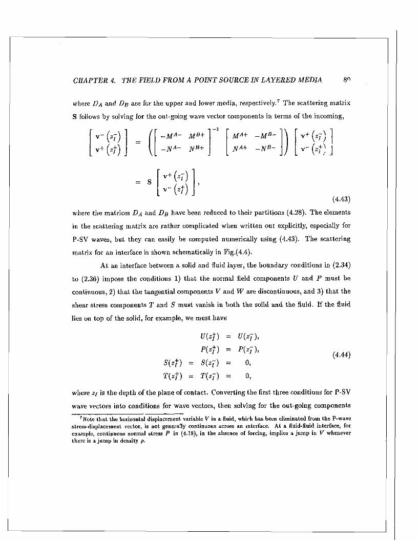
C H A P T E R 4. T H E FIELD F R O M A P O I N T SO U RC E I N L A Y E R E D MED IA 8"
where D a and D b are for the upper and lower media, respectively.7 The scattering m atrix
in the scattering m atrix are ra th e r complicated when w ritten out explicitly, especially for
P-SV waves, but they can easily be computed numerically using (4.43). The scattering
m atrix for an interface is shown schematically in Fig.(4.4).
A t an interface between a solid and fluid layer, the boundary conditions in (2.34)
to (2.36) impose the conditions 1) th a t the norm al field components U and P m ust be
continuous, 2) tha t the tangential components V and W are discontinuous, and 3) th a t the
shear stress components T and S m ust vanish in both the solid and the fluid. If the fluid
lies on top of the solid, for example, we m ust have
where Z[ is the depth of the plane of contact. Converting the first three conditions for P-SV
wave vectors into conditions for wave vectors, then solving for the out-going components
7Note th a t the horizontal displacem ent variable V in a fluid, which has been elim inated from the P-wave stress-displaceincnt vector, is not generally continuous across an interface, A t a fluid-fluid interface, for example, continuous normal stress P in (4.18), in the absence of forcing, implies a jum p in V whenever there is a jum p in density p.
S follows by solving for the out-going wave vector components in term s of the incoming,
(4.43)
where the matrices D a a n d D b have been reduced to their partitions (4.28). The elements
U ( z f ) = U { z j ) ,
P ( z f ) = P ( z j ) ,
S ( z f ) = S ( z j ) = 0,
T ( z f ) = T ( z j ) = 0,
(4.44)
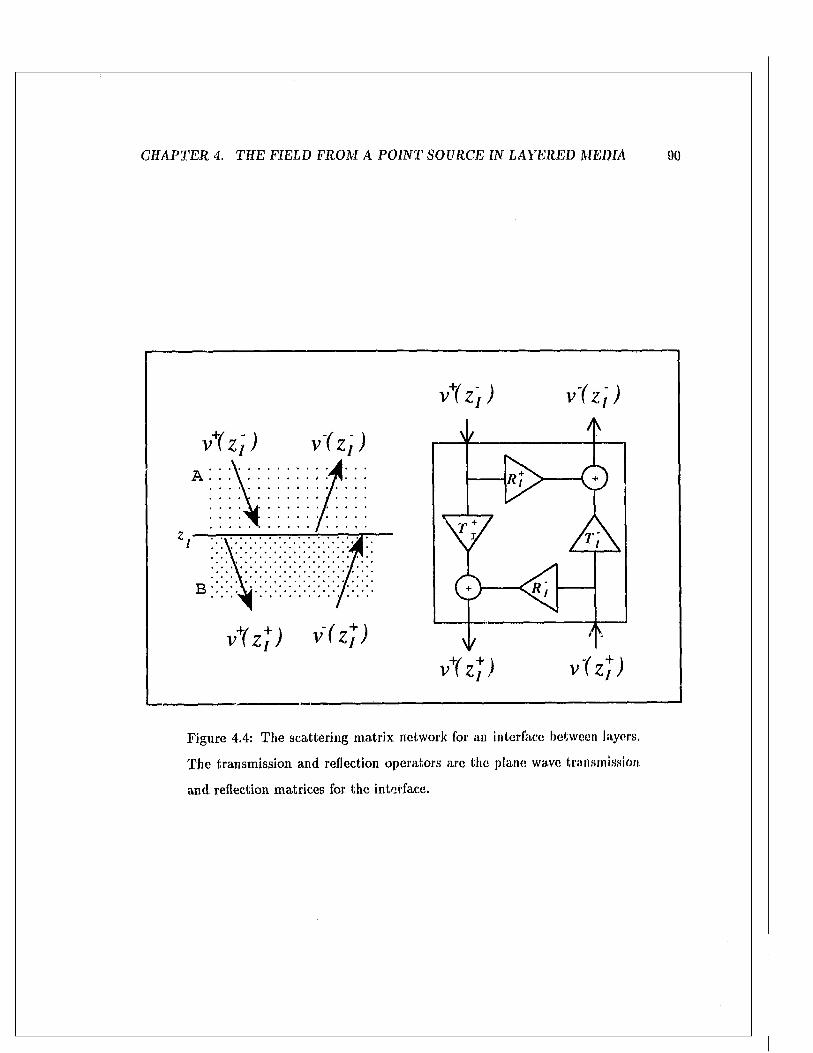
C H A P T E R 4. T H E FIELD F R O M A P O IN T SOURCE IN L A Y E R E D MEDIA 90
vY Z ) ) v ' ( z ] )
Figure 4.4: The scattering m atrix network for an interface between layers.
T he transm ission and reflection operators are the plane wave transmission
and reflection m atrices for the interface.
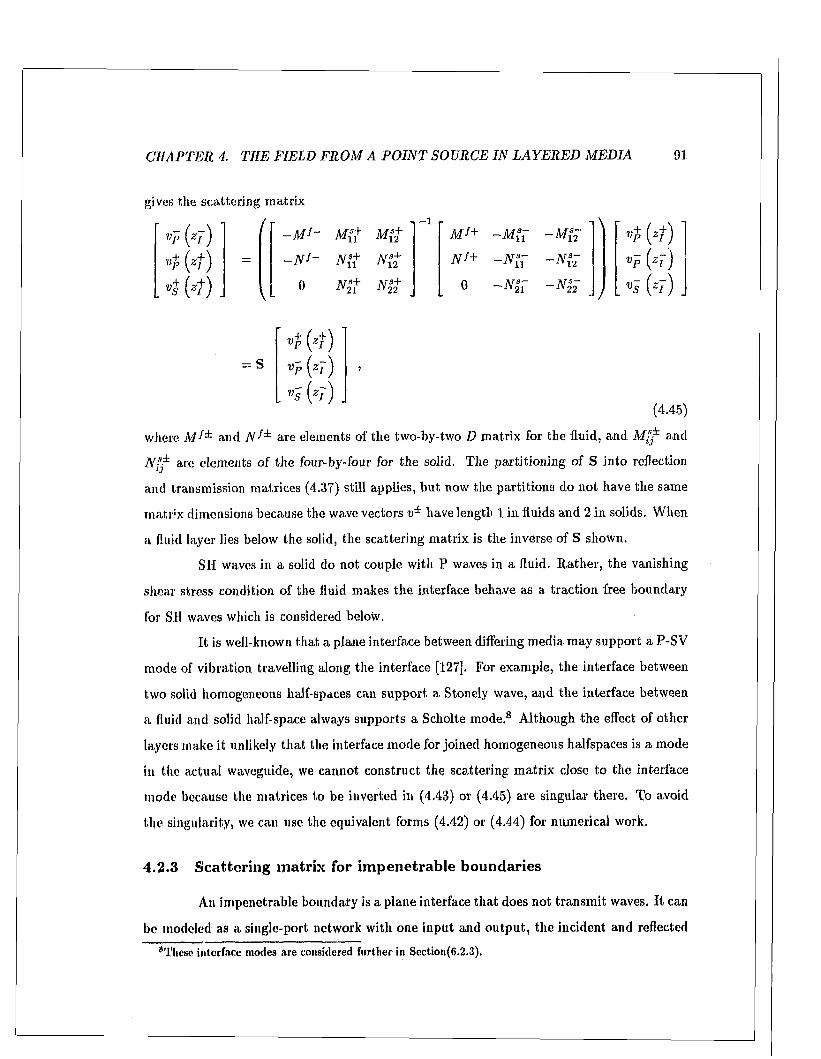
C H A P T E R 4. THE FIELD F R O M A P O IN T SOU RCE IN L A Y E R E D M ED IA 91
gives the scattering m atrix
( * r )/
- M f ~ M4- l
M*+ - m risi
\4 (4 )
4 (4) = arife;l N J + ~ N ( i V p ( z y )
v+ ( * + ) _\
0 Ar| 2+ . 0 ~ n s t ~ N 22 . / _ VS (*7 )
= SVP (4)V p ( z j )
VS (zr ) .(4.45)
where M !± and N ^ are elements of the two-by-two D m atrix for the fluid, and M and
N** are elements of the four-by-four for the solid. The partitioning of S in to reflection
and transm ission m atrices (4.37) still applies, b u t now the partitions do not have the same
m atrix dimensions because the wave vectors v* have length 1 in fluids and 2 in solids. W hen
a fluid layer lies below the solid, the scattering m atrix is the inverse of S shown.
SII waves in a solid do not couple with P waves in a fluid. R ather, the vanishing
shear stress condition of the fluid makes the interface behave as a trac tion free boundary
for SH waves which is considered below.
I t is well-known tha t a plane interface between differing media m ay support a P-SV
m ode of vibration travelling along the interface [127]. For example, the interface between
two solid homogeneous lialf-spaces can support a Stonely wave, and the interface between
a fluid and solid half-space always supports a Scholte mode.8 Although the effect of other
layers make it unlikely th a t the interface m ode for joined homogeneous halfspaces is a mode
in the actual waveguide, we cannot construct the scattering m atrix close to the interface
mode because the m atrices to be inverted in (4.43) or (4.45) are singular there. To avoid
the singularity, we can use the equivalent forms (4.42) or (4.44) for numerical work.
4.2.3 Scattering m atrix for im penetrable boundaries
An im penetrable boundary is a plane interface th a t does not transm it waves. I t can
be modeled as a single-port network with one input and ou tpu t, the incident and reflected
’’These interface modes are considered further in Section(6.2,3).

C H A P T E R 4. T H E FIELD F R O M A P O IN T SOURCE IN L A Y E R E D MEDIA 92
Figure 4.5: T he scattering network for an im penetrable plane boundary is a
reflection operator, which is the plane wave reflection m atrix.
waves, and a single reflection m atrix as shown in Fig.(4.5)
T ra c t io n f re e b o u n d a ry
T he upper interface of an oceanic or seismic waveguide in contact with the a t
mosphere is usually modeled by a traction free boundary where P , S , T — 0 . Setting the
traction portion t = 0 in (4.32) we find
u p p e r b o u n d a ry
»’ (<■)
l o w e r b o u n d a r yV+ 'z)
o = JV+v+(j2) + JV -V (z) (4.46)
where z is the depth of the boundary. T he reflection m atrix for a lower (+ ) and upper (" )
free interface are therefore
R + = - ( j V - ) “ 1 1V+ = ( R - ) " 1 . (4.47)

C H A P T E R 4. T H E FIELD F R O M A P O IN T SOURCE IN L A Y E R E D M ED IA 93
Using the expressions for in (4.29), we can simplify R * = - 1 for P waves in a fluid,
and R ^ = 1 for SH waves in a solid.
I t is well-known th a t a free boundary on a homogeneous solid half space supports
a P-SV interface wave, the Rayleigh mode [127].9 Here again, the effect of o ther layers on
the wave m otion m ake it unlikely th a t the Rayleigh mode of the homogeneous half space is
a mode of v ibration in the waveguide, bu t we cannot covstruct the reflection m atrix (4.47)
close to the Rayleigh m ode because are singular there, and then it is best to use (4.46)
in the numerical com putations.
Rigid-welded boundary
T he waveguide m ay be bounded below by a rigid, displacement free boundary at
depth 2. For a solid layer in welded contact U , V , W = 0. Setting the displacement partition
w = 0 in (4.32) we find
0 = Af+ v + (2) 4- M ~ v ~ ( z ) . (4.48)
T he plane wave reflection m atrices for a lower (+) and upper (“ ) rigid interface are therefore
R+ = - { M ~ ) - 1 M+ ^ (R“)- 1 . (4.49)
Using the expressions for M * in (4.29) we can simplify R ^ = - 1 for SH waves in a solid.
T he rigid boundary on an infinite solid half space supports a P-SV interface mode, a lesser
known leaky (im proper) counterpart of the Rayleigh mode,10 a t which for P-SV waves
are singular.
Rigid-lubricated boundary
A rigid boundary makes frictionless contact with an inviscid fluid layer, and the
vertical (norm al) displacement U = 0, while the horizontal (tangentia l) displacement V for
P waves remains unconstrained. For P waves in fluids we find
R + = ~ ( M - ) " 1M + = ( R - ) -1 = 1. (4.50)
®Thc Rayleigh wave is considered further in Section(6.2.3).10I have not Come across these inodes in the literature. For lack of a b e tte r name, I call this the Rayleigh
mode of the second kind in Section(6.2.3).
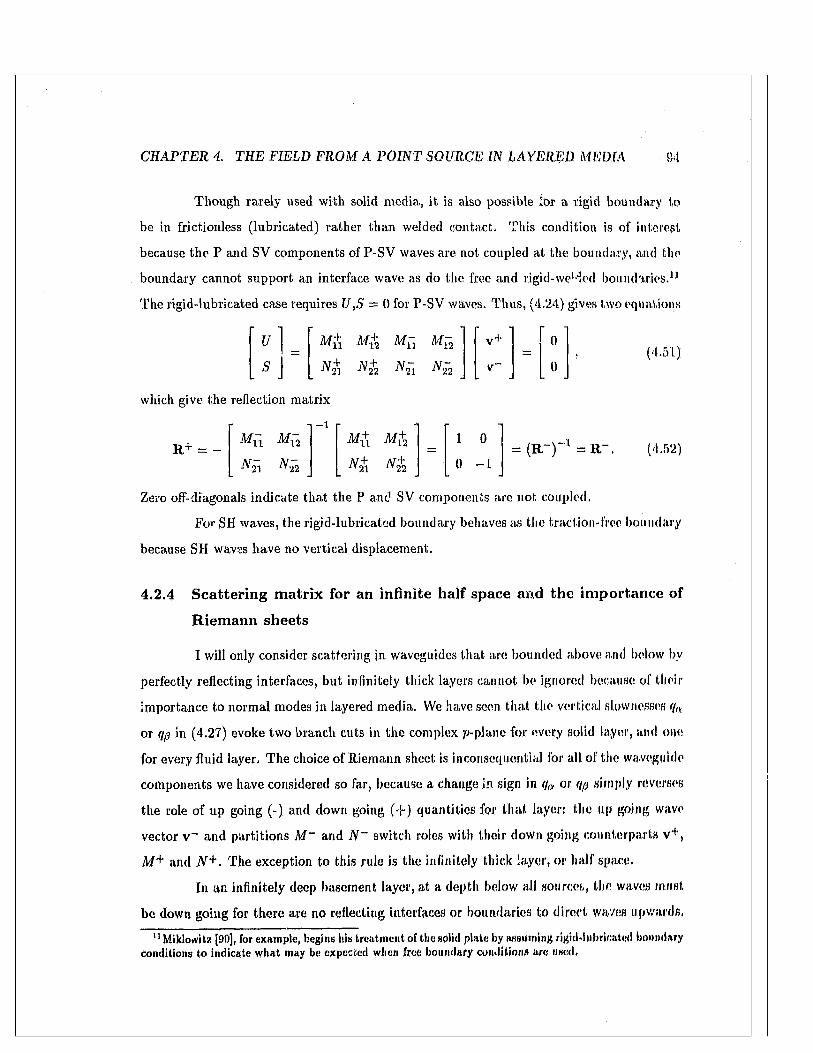
C H A P T E R 4. T H E FIELD F R O M A P O IN T SOURCE IN L A Y E R E D MEDIA 94
Though rarely used w ith solid media, it is also possible lor a rigid boundary to
be in frict.ionless (lubricated) ra ther than welded contact. This condition is of interest
because the P and SV components of P-SV waves are not coupled at the boundary, and the
boundary cannot support an interface wave as do the free and rigid-we’ded boundaries.11
The rigid-lubricated case requires U,S = 0 for P-SV waves. Thus, (4.24) gives two equations
u M u M^z M u M n V + 0
s No j -/V'22 ^21 ^22 V“ 0
which give the reflection m atrix
R+ = -Mii Mn
- l +3i
>o+
t
I 0
1 f*H feTi 1 " S+ 2 0 -1
Zero off-diagonals indicate th a t the P and SV components are not coupled.
For SII waves, the rigid-lubricated boundary behaves as the traction-free boundary
because SH waves have no vertical displacement.
4.2.4 Scattering m atrix for an infinite half space and the im portance of
Riem ann sheets
I will only consider scattering in waveguides tha t are bounded above and Inflow by
perfectly reflecting interfaces, but infinitely thick layers cannot be ignored because of their
im portance to norm al modes in layered media. We have seen th a t the vertical slownesses
or qp in (4.27) evoke two branch cuts in the complex p-plane for every solid layer, and one
for every fluid layer, T he choice of Riem ann sheet is inconsequential for all of the waveguide
com ponents we have considered so far, because a change in sign in qa or qp simply reverses
the role of up going (-) and down going (•[-) quantities for th a t layer: the up going wave
vector v~ and partitions M ~ and N ~ switch roles with their down going counterparts v+,
M + and JV+. The exception to this rule is the infinitely thick layer, or half space.
In an infinitely deep basement layer, a t a depth below all sources, the waves must
be down going for there are no reflecting interfaces or boundaries to direct waves upwards.
"M ikiow itz [90], for example, begins his treatm ent of the solid plate by assuming rigid-lubricated boundary conditions to indicate w hat may be expected when free boundary conditions are used.
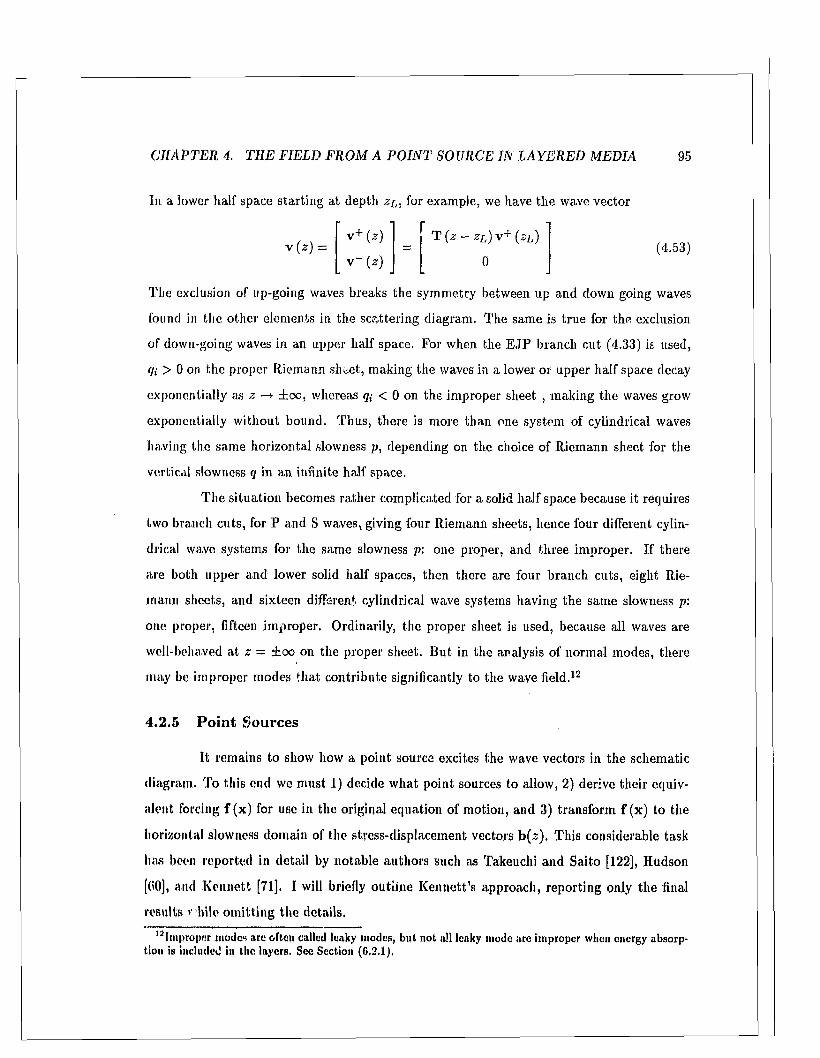
C H A P T E R 4. T H E FIELD F R O M A P O I N T SO URCE IN L A Y E R E D MED IA 95
In a lower half space starting at depth z l , for example, we have the wave vector
1+>t
T ( z - zL) v + (z i )
1V1>
t
-----1
o
I
The exclusion of up-going waves breaks the sym m etry between up and down going waves
found in the other elements in the scattering diagram. The same is true for the exclusion
of down-going waves in an upper half space. For when the E JP branch cut (4.33) is used,
<li > 0 on the proper Riemann sheet, making the waves in a lower or upper half space decay
exponentially as z —»■ ±oo, whereas qi < 0 on the im proper sheet , making the waves grow
exponentially w ithout bound. Thus, there is more than one system of cylindrical waves
having the same horizontal slowness p, depending on the choice of Riemann sheet for the
vertical slowness q in an infinite half space.
T he situation becomes ra ther complicated for a solid half space because it requires
two branch cuts, for P and S waves, giving four Riemann sheets, hence four different cylin
drical wave systems for the same slowness p : one proper, and three im proper. If there
are both upper and lower solid half spaces, then there are four branch cuts, eight Rie
mann sheets, and sixteen different cylindrical wave systems having the same slowness p:
one propei1, fifteen im proper. Ordinarily, the proper sheet is used, because all waves are
well-behaved a t z = ±oo on the proper sheet. B ut in the analysis of norm al modes, there
may be im proper modes th a t contribute significantly to the wave field.12
4.2.5 Point Sources
I t remains to show how a point source excites the wave vectors in the schematic
diagram. To this end we m ust 1) decide w hat point sources to allow, 2) derive their equiv
alent forcing f (x) for use in the original equation of motion, and 3) transform f (x) to the
horizontal slowness domain of the stress-displacement vectors b{z). This considerable task
has been reported in detail by notable authors such as Takeuchi and Saito [122], Hudson
[00], and K ennett [71]. I will briefly outline K ennett’s approach, reporting only the final
results r hile om itting the details.
^Im proper modes ate often called leaky modes, bu t not all leaky mode are im proper when energy absorption is included in the layers. Sec Section (6,2.1).
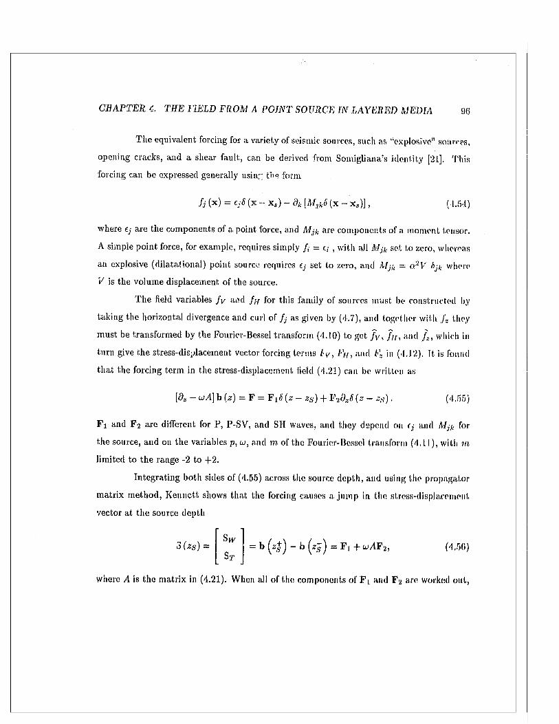
C H A P T E R 4. TH E FIELD F R O M A P O IN T SO URCE IN L A Y E R E D MEDIA 9(5
The equivalent forcing for a variety of seismic sources, such as “explosive” sources,
opening cracks, and a shear fault, can be derived from Somigliana’s .identity [21]. This
forcing can be expressed generally iisiny the form
where ej are the components of a point force, and Mjk are components of a moment tensor.
A simple point force, for example, requires simply /; = e,- , with all Mjk set to zero, whereas
an explosive (dilatalional) point source requires e/ set to zero, and Mjk - « 2P /ijk where
V is the volume displacement of the source.
T he field variables f y and / ; / for this family of sources must, be constructed by
taking the horizontal divergence and curl of f j as given by (4.7), and together with f g they
m ust be transform ed by the Fourier-Bessel transform (4.10) to get f y , / / / , and / , , which in
tu rn give che stress-displacement vector forcing term s b y , /')/, and Fz in (4.12). ft is found
th a t the forcing term in the stress-displacement field (4.21) can be written as
F j and F 2 are different for P, P-SV, and SH waves, and they depend on ( j and Mjk for
the source, and on the variables p, u>, and m of the Fourier-Hesscl transform (4.11), with m
lim ited to the range -2 to +2.
Integrating both sides of (4.55) across the source depth, and using the propagator
m atrix m ethod, K ennctt shows tha t the forcing causes a jum p in the stress-displacement
vector at the source depth
where A is the m atrix in (4.21). When all of the components of F i and Fy are worked out,
f j ( x ) = e;S ( x - x s ) - dk [MjkS (x - x s )] (1.54)
[dz - u A ] b (z) = F = F ;l<5 (z - z s ) + F 2 0 J (z - zs ) . (4,55)
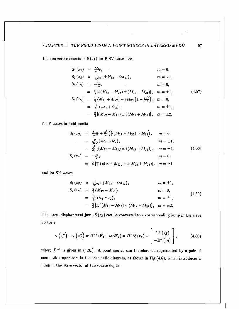
C H A P T E R 4. T H E FIELD F R O M A P O I N T SO URCE I N L A Y E R E D M E D IA 97
the non-zero elements in S (25) for P-SV waves are
s . f e ) = f f , TO = 0,
$2 fa s) = 2 /?* faA /13 - iMiz) j TO = . . I ,
S3 fa,S') = TO — 0,
= 2 [i (Mz 2 - A/23) ± (A/33 - M31)] , 771 = ±1 , (4.57)
s,, (zs) = t ( M n + M 2 2 ) - p M :ia( l - ^ ) , TO = 0,
= 2b (T £i + *e2) , TO = ±1,
= 4 K A/22 - A fn ) ± i (A/12 + A/21) ] , m = ± 2;
for P waves in fluid media
Si fa s) — ( | (A/11 + A/22) — A/33) , TO = 0,
= 2 (^ 1 + ^ 2) , TO = ±1,
= ((A/22 - M u ) ± i (A/12 + A/21)) > t o - - ± 2, (4.58)
S afas) = TO = 0,
— 2 ["F (^1 3 + A/31) + i (A/32 + A/23)] j to = ±1;
and for SH waves
Si fas) = 5^2 ^TA/23 - iA/13) , TO = ±1 ,
S2 fas) = K M 12- M 21) ,
= ^ ( * c i ± e a ) ,
TO = 0,
TO ~ ±1 ,(4.59)
= 2 [±1 (/Vfii - A/22) -t (A/12 + Af2i ) ] , to = ±2.
The stress-displacement jum p S ( zs) can be converted to a corresponding jum p in the wave
vector v
v ( 4 ) - v ( * j ) = D ~ l (F i + " 4 F 2 ) = D - ' S ( zs) =£ + fas)
_ - £ - f a s ) _(4.60)
where D ~ l is given in (4.31). A point source can therefore be represented by a pair of
sum m ation operators in the schematic diagram , as shown in Fig.(4.6), which introduces a
jum p in the wave vector at the source depth.
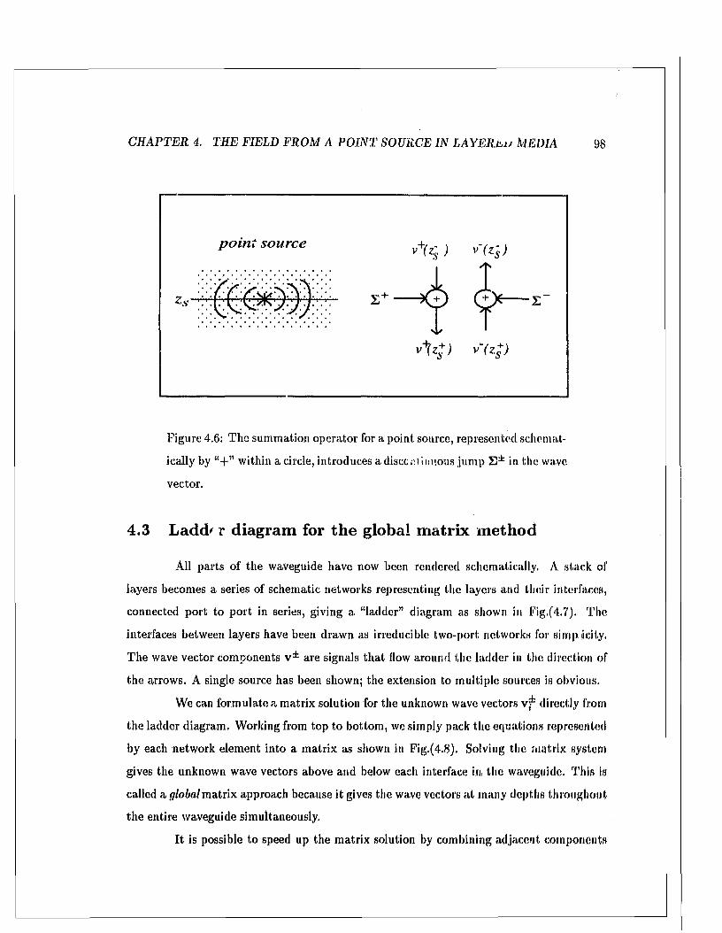
C H A P T E R 4. T H E FIELD F R O M A P O IN T SOURCE IN L A Y E R h u MEDIA 98
p o i n t s o u r c e
Figure 4.6: T he summation operator for a point source, represented schemat
ically by within a circle, introduces a discern muons jum p E * in the wave
vector.
4.3 Ladd' r diagram for th e global m atrix m ethod
All parts of the waveguide have now been rendered schematically. A stack of
layers becomes a series of schematic networks representing the layers and their interlaces,
connected po rt to po rt in series, giving a “ladder” diagram as shown in Fig.(4.7). The
interfaces between layers have been draw n as irreducible two-port networks for simplicity.
The wave vector components v * are signals th a t flow around the ladder in the direction of
the arrows. A single source has been shown; the extension to m ultiple sources is obvious.
We can form ulate a m atrix solution for the unknown wave vectors v f directly from
the ladder diagram . Working from top to bottom , we simply pack the equations represented
by each netw ork element into a m atrix as shown in Fig.(4.8). Solving the m atrix system
gives the unknown wave vectors above and below each interface in, the waveguide. This is
called a global m atrix approach because it gives the wave vectors a t many '
the entire waveguide simultaneously.
I t is possible to speed up the m atrix solution by combining adjacent components
8035641141
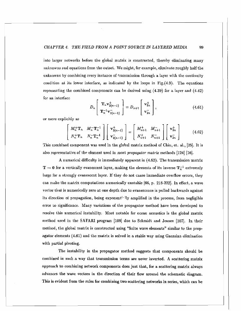
C H A P T E R 4. TH E FIELD F R O M A P O IN T SO U RCE IN L A Y E R E D M ED IA 99
into larger networks before the global m atrix is constructed, thereby elim inating m any
unknowns and equations from the outset. We m ight, for example, elim inate roughly half the
unknowns by combining every instance of transm ission through a layer w ith the continuity
condition a t its lower interface, as indicated by the loops in Fig.(4.9). The equations
representing the combined Components can be derived using (4.39) for a layer and (4.42)
for an interface
D n ■ D n+i V2n
. T n 1V2"(n_ 1) _. V2_" .
(4.61)
or more explicitly as
M + T „ M - T - 1
1< !£.+
3 1
1M~+1
1< 5?
+l
. A + T „ N ~ T ~ l _ . V2(n—1) . . K +i . . V2” .
(4.62)
This combined com ponent was used in the global m atrix m ethod of Chin, et. al., [25]. I t is
also representative of the element used in m ost propagator matrix m ethods [124] [16].
A numerical difficulty is im m ediately apparent in (4.62). The transm ission m atrix
T —» 0 for a vertically evanescent layer, m aking the elements of its inverse T ~ x extremely
large lor a strongly evanescent layer. If they do not cause im m ediate overflow errors, they
can make the m atrix com putations numerically unstable [66, p. 218-222]. In effect, a wave
vector th a t is numerically zero at one depth due to evanescence is pulled backwards against
its direction ol propagation, being exponent5 Hy amplified in the process, from negligible
error to significance. Many variations of the propagator m ethod have been developed to
resolve this numerical instability. Most notable for ocean acoustics is the global m atrix
m ethod used in the SAFARI program [109] due to Schmidt and Jensen [107]. In their
m ethod, the global m atrix is constructed using “finite wave elem ents” similar to the prop
agator elements (4.61) and the m atrix is solved in a stable way using Gaussian elim ination
with partia l pivoting.
T he instability in the propagator m ethod suggests th a t components should be
combined in such a way that transm ission term s are never inverted. A scattering m atrix
approach to combining network com ponents does just th a t, for a scattering m atrix always
advances the wave vectors in the direction of their flow around the schematic diagram .
This is evident from the rules for combining two scattering networks in series, which can be
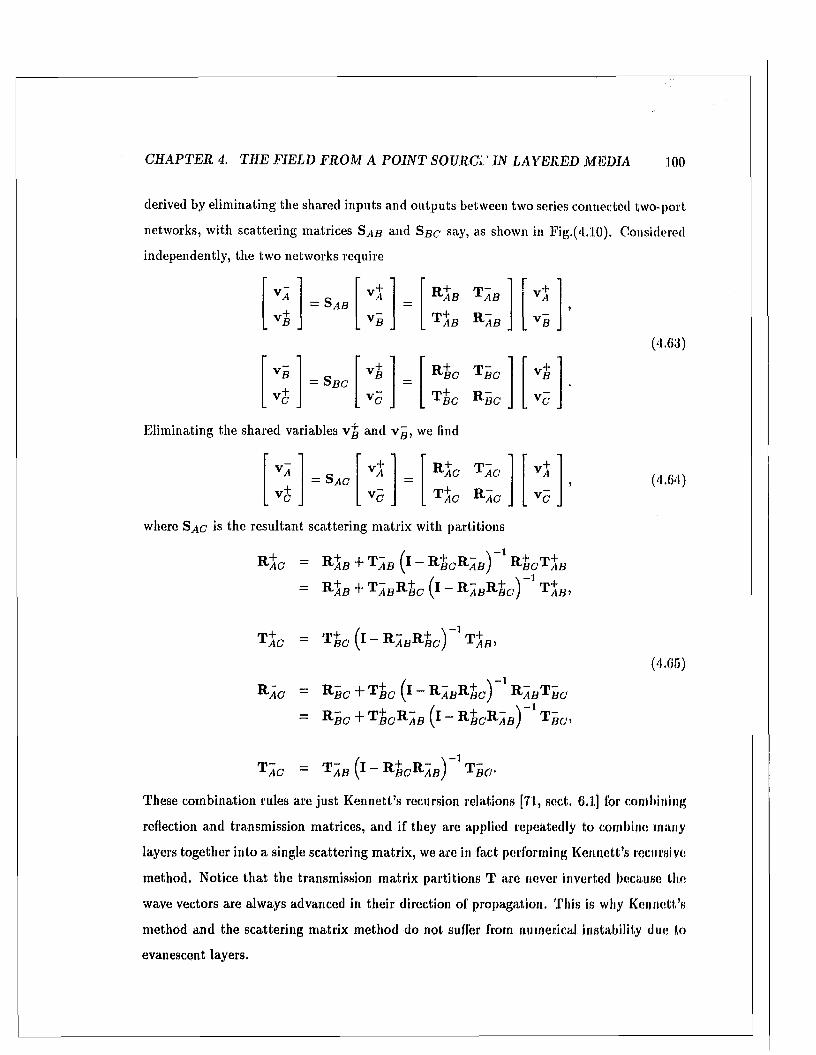
C H A P T E R 4. T H E FIELD F R O M A P O I N T SOURCE I N L A Y E R E D MEDIA 100
derived by elim inating the shared inputs and outputs between two series connected two-port
networks, with scattering matrices S AB and Sb c say, as shown in Fig.(4.10). Considered
independently, the two networks require
V A
. V * .
= S a bv l
. .
= ® 7 lB
T a b
T a b
^■AB
V A
. V «
V B = S BCV B
. V 5 .
=r b c
^ b c
T BC
® -B C _
v fl
. .
Eliminating the shared variables v B and vB , we find
V .4= S a c
1 1
10 >
>i
... i
= ® -a c
. T t o
T a c '
®71C
v j
. v 5 .
where Sac is the resultant scattering m atrix with partitions
® v i c = R A B + T A B ( * ~ R B O R ^ e ) R B C T AAB
~ R AB + T /1BR BC ( l “ R ViBR f lc ) T AB’
R AC - R flC + T BC (* ~ ^ / t f l^ B C ') R ABT BC
= R BC + T BC®VtB (* - R BCR /lf l) T BC>
(4.03)
(4.64)
(4.65)
t a c ~ ^ B ( * ~ ^ B c ^ v i s ) T B<r/-
These com bination rules are ju s t K ennett’s recursion relations [71, sect. 6.1] lor combining
reflection and transm ission m atrices, and if they are applied repeatedly to combine many
layers together into a single scattering m atrix , we are in fact performing K ennett’s recursive
m ethod. Notice th a t the transm ission m atrix partitions T are never inverted because the
wave vectors are always advanced in their direction of propagation. This is why K ennett’s
m ethod and the scattering m atrix m ethod do not suffer from numerical instability due to
evanescent layers.

C H A P T E R 4. T H E FIELD F R O M A P O IN T SO URCE IN L A Y E R E D M ED IA 101
In field com putations we will need to com pute the wave vector a t a depth within
a combined elem er.\ The scattering m atrix for the combined element m ust then be split
into two scattering matrices at the desired depth. Hence, the wave vectors at za and z c in
Fig.(4.10) are now known, and we m ust solve (4.63) for the interm ediate wave vector v b
( l - T AB ( l ~ ^ B ^ - B c ) B ^E C
( i - R b C ’® v 1 b ) ^BC^AB ( * _ ® - B C ® v 1 b ) T bc(4.66)
Here again, term s like T -1 do not occur, so evanescent layers do not cause numerical
instability.
VB II
. V«
4.4 A single source and receiver
Using a scattering m atrix approach, or equivalently, K ennett’s recursive scheme,
the ladder diagram for any waveguide can be reduced to its simplest form consisting of the
source and an upper and lower reflection m atrix as shown in Fig. (4.11). A m atrix equation
for the waveguide can then be w ritten directly from the diagram
(4.67)* R-os
1< + CO
+«
£+
“ R-SX 1 1 ■ 1
PP
■ £ -
The solution is r. - i
£ + + R 0-s £ -
R + ^ + E-(4.68)
v + ( 4 ) = ( i - R o s R s J
v_ (% ) = ( l ~ R -sx^os)
which can be in terpreted physically using “rays” [71] if the left hand side is expanded in
the series
+ •••') fsT + R0<?£"1,(4.69)
v+ ( 4 ) - f 1 + R 0S&SL + (R-OS^Sl) + • • -j [s-r + R 0s S “ ] ,
v - ( ^ ) = ( i + R |bRos+ ( r | xRos) 2 + ---) [r J£S+ + E-] .
The terms in the series give first a direct source contribution, then a pair of reflections, then
reflections of those reflections, and so on. In this way, ( i - R “SR ^ ) 1 and ( i - R j LR “s )
account for the reverberation in the waveguide a t the source depth , and they are often called
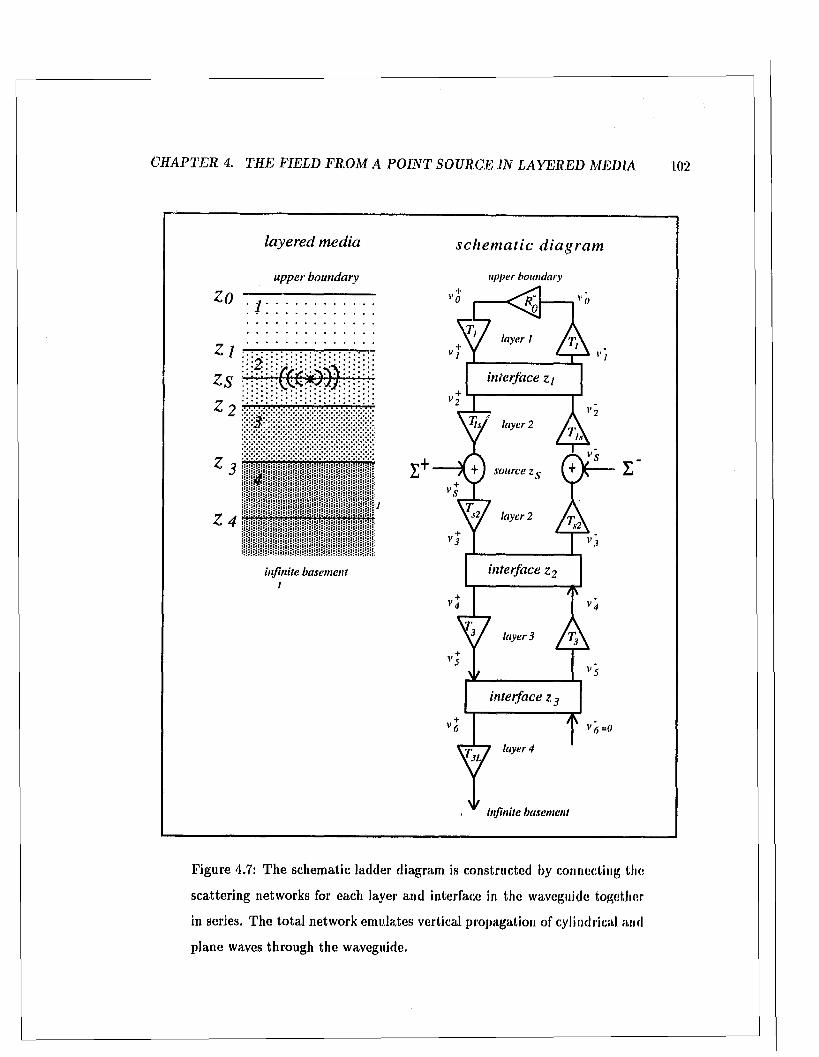
C H A P T E R 4. T H E F IE L D F R O M A P O I N T S O U R C E IN L A Y E R E D M E D IA 102
l a y e r e d m e d i a
upper boundary
infinite basement I
s c h e m a t i c d i a g r a m
upper boundary
layer I
layer 2
+ ) source z
layer 2
layer 3
layer 43L
infinite basement
interface z. /
interface z.2
interface z
Figure 4.7: T he schematic ladder diagram is constructed by connecting the
scattering networks for each layer and interface in the waveguide together
in series. The to ta l network em ulates vertical propagation o" „ " 1 !cal and
plane waves through the waveguide.
5152
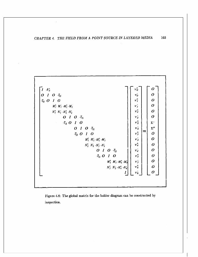
C H A P T E R 4. TH E FIELD F R O M A P O IN T SO U RCE IN L A Y E R E D M E D IA 103
I -*2 V o O
O I O -Tol v~o O
■T0I O I O V+l O
M; M'l -M2 -M~2 V ) O
N ) N ] - N \ -N 2 V~2 O
O I O -TIS V 2 O
-Tls O I O Vs V
O I O -ts2 Vs L+
-tS2 O I 0 Vs O
M\ M2 -M] -M3 v; O
N \ N 2 -N +3 -N } V 4 O
O I O -T23 V 4 O
■t23 O I O V5 O
M*3 M3 -M4 -M4 V} O
N +s N s -N +4 -N 4 Vfi O
I v 'e O
Figure 4.8: T he global m atrix for the ladder diagram can be constructed by
inspection.
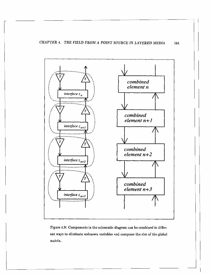
C H A P T E R 4. TH E FIELD F R O M A P O IN T SO U RCE IN L A Y E R E D MEDIA m
A
interface z n
interface z n+l
T \ \
interface z n+2
4 ....... '
v k
interface z n+3
\ /combined element n
\
/
/
\
combined element n+J
\
/
(
\
combined element n+2
\
/
/
\
combined element n+3
/
Figure 4.9: Com ponents in the schematic diagram can be combined in differ-
ent ways to elim inate unknown variables and compress the size of the global
m atrix.
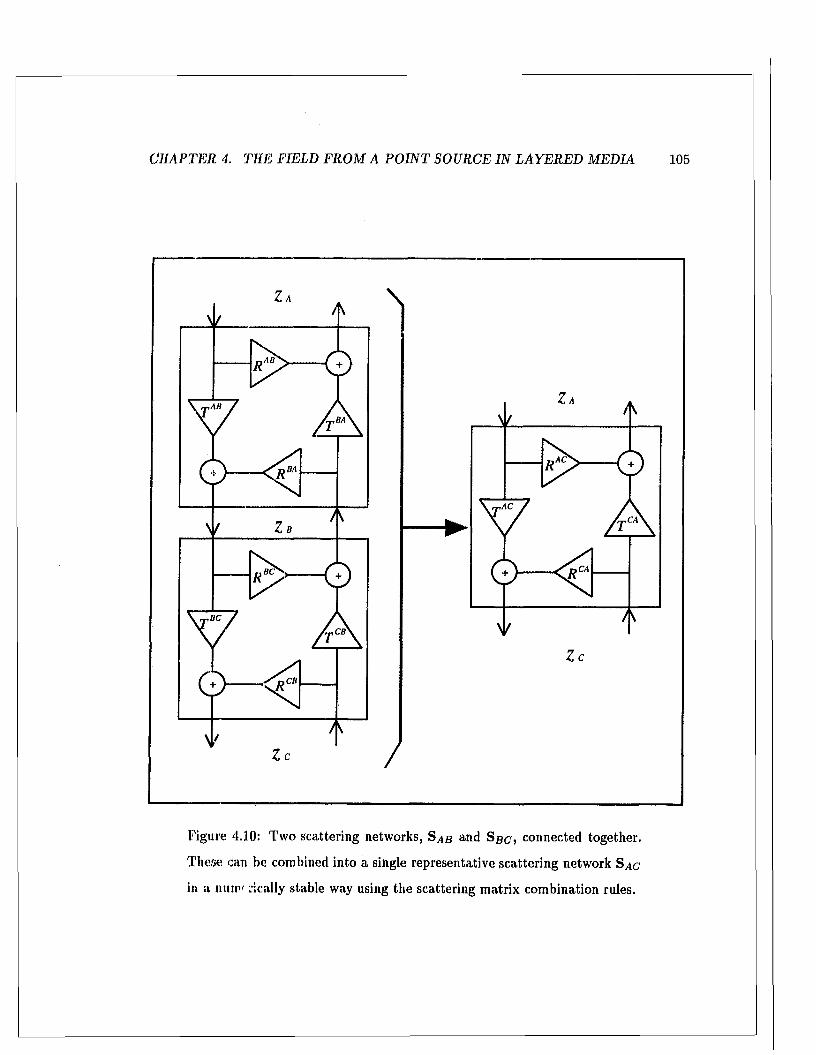
C H A P TE R 4. TH E FIELD F R O M A P O IN T SO URCE IN L A Y E R E D M ED IA 105
,AC
,ACCA
►
CA
,AB
,ABBA
BCCB
Figure 4.10: Tw o scattering networks, and S aa? connected together.
These can be combined into a single representative scattering network S a c
in a nunv I'ically stable way using the scattering m atrix com bination rules.
C H A P T E R 4. T H E FIELD F R O M A P O IN T SO URCE IN L A Y E R E D M ED IA 106
the reverberation operators. Notice th a t reverberation operators also appear in the recursion
relations (4.6o) due to the reverberation between the connected networks.
To derive the wave vector at some receiver depth z r , we m ust split the waveguide
at zR and combine all of the components between z r and z s in to a single scattering m atrix
Sr s - A ll layers above and below both the source and receiver can again be combined into
single reflection m atrices. Fig.(4.12) shows the schematic diagram when z r < z s . By
inspection we can write
v O h) = T fi5v~ [zs ) + R + s.v+ (zR ) .
Solving for v~ ( z r ) and using v + ( z r ) - R q r V ~ ( z r ) gives
(4.70)
v O ft) = <R Oil
(* ~ RAsRor) T rs M
R OR( * - R r s ' R q r ) t / i s ( l - R + R0- ,)" '[R + ^ + + E-
(4.71)
Fig. (4.12) also shows the situation when z r > zs , in which case
v ( z r ) = <
R rl( l “ R - S r R r r ) T 5 R | v + ( ZS )
R rl(4.72)
Here again the expressions can be in terpreted physically using rays.
4.5 R ecovery o f th e to ta l elastic field
We m ust invert the Fourier-Beasel transforms (4.11) to recover the clastic wave
field from the stress displacement vector. This inversion determines the range o< values for
u>, p and rn for which the stress displacement vector b ( z n ) -and hence, the wave vector
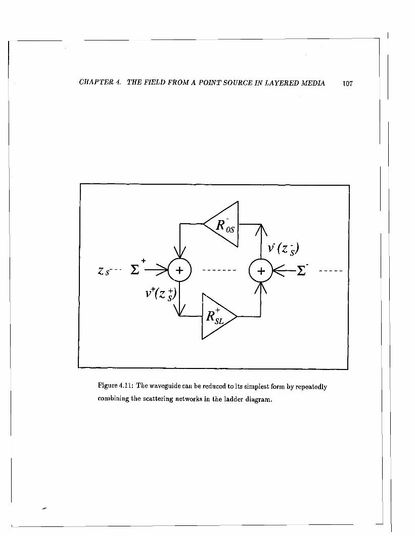
C H A P T E R 4. TH E FIELD F R O M A P O IN T SO U RC E IN L A Y E R E D M ED IA 107
OS
S L
Figure 4.11: T he waveguide can be reduced to its simplest form by repeatedly
combining the scattering networks in the ladder diagram .
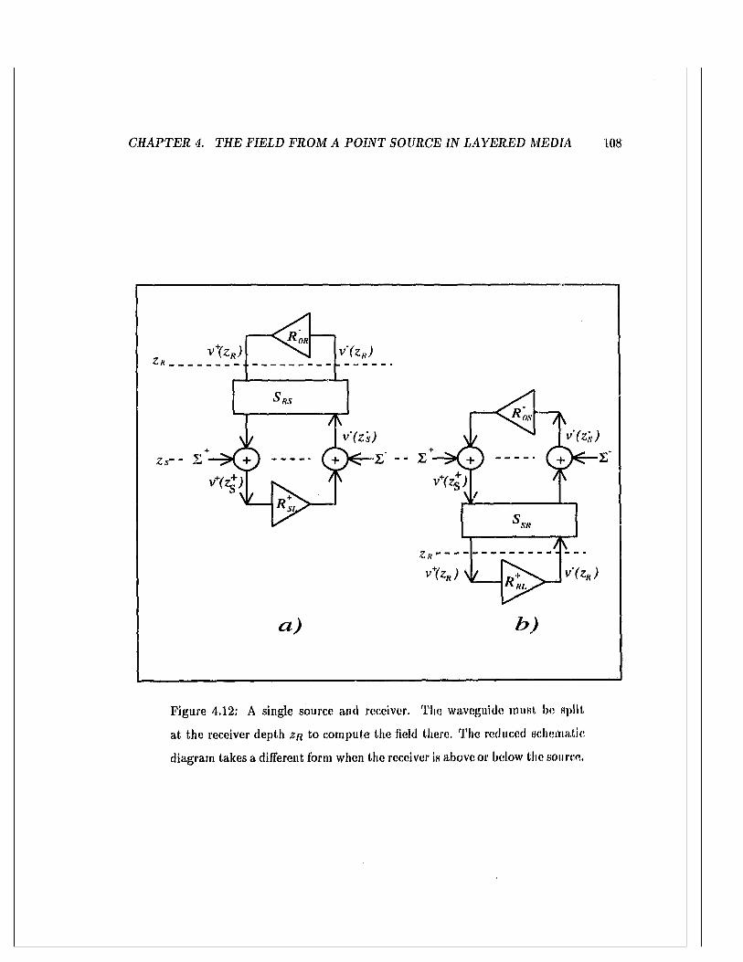
C H A P TE R 4. TH E FIELD F R O M A P O IN T SO URCE IN L A Y E R E D MEDIA 108
OR
Z r
RS
Zs
RL
a) b)
Figure 4.12: A single source and receiver. The waveguide m ust be split
a t the receiver depth zr to com pute the field there. The reduced schematic
diagram takes a different form when the receiver is above or below the source.
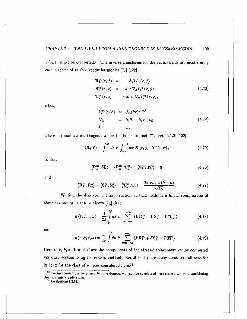
C H A P TE R 4. TH E FIELD F R O M A P O IN T SO U RCE IN L A Y E R E D M ED IA 109
v ( z / i ) mus t be com puted .13 The inverse transforms for the vector fields are most simply
cast in term s of surface vector harmonics [71] [122]
R %(r,4>) = e zY£n (r,<j>),
S f(r,cf>) = k - ' V h Y f i r , ® , (4.73)
= —gz X V hY™ ( r , <f> ) ,
whereY™ (''', <•/>) - Jm(kr)e im,l‘,
V/t = e rdr + (4.74)
k = up
These harmonics are orthogonal under the inner product [71, sect. 2.1.2] [122]
r oo /’■Hr(X , Y ) = / dr r # X (r, t/>) ■ Y * (r, cf>), (4.75)
J 0 J - 7T
io that
( R £ \ s n = = ( S f , T f ) = 0 (4.76)
and
(R fc \R «) = <Sg*,S£) = < T £ ,T £ ) = (4.77)v k ,K
W riting the displacement and traction vertical fields as a linear com bination of
these harmonics, it can be shown [71] th a t
i 7 +cou(r,4>,z,u>) = — I d k k £ ( U R f + V S f + W T f ) (4.78)
q 771 = -O O
andu 7 +0°
t(r,<j),z,u})= — I dk k £ (P R f + S S f + T T f ) . (4.79)q 77l = —0 0
Ifere U , V ,P , S ,W and T are the com ponents of the stress-displacem ent vector com puted
via wave vectors using the m atrix m ethod. Recall th a t these com ponents are all zero for
|m | > 2 for the class of sources considered here .1'1
l3Thc inversion from frequency to time domain will not be considered here since I am onlv considering the harmonic steady sta te .
14See Sectional.2.5).
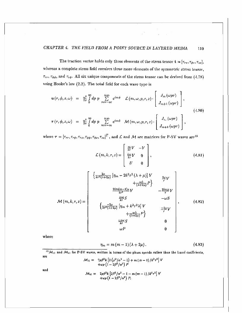
C H A P T E R 4. TH E FIELD F R O M A P O IN T SO U RCE IN L A Y E R E D M EDIA 110
T he traction vector holds only three elements of the stress tensor t = [rrs , r,/,., r se],
whereas a complete stress field requires three more elements of the symmetric stress tensor,
Trr, T<t>$, and r r^. All six unique components of the stress tensor can be derived from (-1.78)
using Hooke’s law (2.2). The to tal field for each wave type is
ihM u and M m for P-SV waves, w ritten in term s of the phase speeds rather than the Lamd coefficients, are
(•1.80)
T(r ,<f>,e,w) = ' ^ f <lP p E M ( m , u ,p , r , z ) •0 m~ °° Jm+1 (upr)
where r = [r,.,., rT$, rrz, t^ , , and C and M are matrices for P-SV waves a re15
kr ’ '
C ( m , k , r , z ) = i s i y 0 ,
U 0
& V - V
(4.81)
{ w u W ) b n ~ 2k 2 r 2 (A + //)] V 111 v
M (m, k, r, z ) = (4.82){ ^ (.\+ W ) b n + k?r2\ \ V -'Li v
r(A+2,1)
0
o
where
Vm = m (to - 1) (A + 2 / t ) . (4.83)
M n = n p ^k [2 (/P/a2 - l) + m (,n - 1) / * V ] V + u p ( l - 2/32/ o 2) P
andM u = IpfPk [2/?7«2 - 1 - m (m - I) /* V ] V
+wp( 1 — 2/3s/»2) P,

C H A P T E R 4. TH E FIELD F R O M A P O IN T SO U RC E IN L A Y E R E D M ED IA
For P waves, C is the same as for P-SV waves with V = -kP/(u>p) (not a t the source
and
r 1 0
for SH .vaves
M (m , k, r, z) — u P
0 0
0 0
1 0
0 0
1 0
£ ( m , k , r , z ) = W
imkrhr
o o
M (m , k , r , z ) =
H Wkr22 i\m i j y
i [k2 + (1 - m)] W - f W
0i win m kr 1
kr2
urn mkr
2ip.mru T
0
W
i l l
depth)
(4.84)
(4.85)
(4.86)
112
C h a p t e r 5
M odes in layered m edia
We have seen th a t the field due to a harmonic point source can be computed
by evaluating the Fourier-Bessel transforms (4.80). Perhaps the most powerful analytic
m ethod for evaluating such integrals is the residue theorem, which reduces the integral to
a sum over the residues of poles in the complex plane, offering an alternative to direct
numerical integration. In this chapter it is shown tha t the poles of the Fourier-Bessel
transform s are the normal modes of the waveguide, and the sum of the residues is th
sum of th e contribution of each norm al m ode to the field. T he m otivation for the switch
is the prospect of greater com putation speed, since the bulk of the mode com putations
can be carried out beforehand and saved for ready access during the BIE method. The
norm al m ode approach is particularly efficient when the receiver is far from a source, when
relatively few (propagating) modes contribute significantly.1 Close to the source, however,
all advantage may be lost because many short range (evanescent) modes are needed.
T he modal representation of the field begins with a search for poles in the corn
plex slowness plane, or, what am ounts to the same thing, a search for the roots of the
denom inator of the Fourier-Bessel integrand. A com puter search for the complex roots of
any complicated function is difficult and uncertain; difficult because we must by analysis
deduce roughly where and how close the roots are likely to be to direct the com puter search
'W hen describing a mode search, it is impossible to avoid distinguishing between modes such as propagating, evanescent and leaky modes, bu t it would detrac t to define them here. All inode names printed ill italics are defined later in C hapter S.
C H A P TE R 5. M O D ES IN L A Y E R E D M ED IA 113
with confidence; and uncertain because we cannot, in general, verify conclusively th a t all of
the roots have been found .2 The problem is worse in the search for modes because different
characteristic equations for roots result in different layers in the waveguide; all modes cannot
be detected a t a single depth. In an exhaustive mode search, we m ust therefore scan m any
different characteristic equations for roots simultaneously. Existing norm al mode programs
simplify m atters by aiming to find ju st the propagating modes whose vibrations dom inate
the total field far from a source, and in ocean acoustics they are often lim ited to modes
whose vibrations extend significantly into the w ater column. This partia l approach is effi
cient and accurate when the source and receiver are positioned accordingly,3 but in the BIE
method, the receiver is the boundary integration variable and the source the com putation
point, and they come very close together—actually touching in the lim it in the surface-field
equation—making short-acting evanescent modes indispensable. The receiver m ay also lie
within the sea floor or an ice plate, where modes confined within those solid m edia dom inate
the field, making it necessary to include modes vibrating outside the w ater column. A new
exhaustive search m ethod was therefore required.
A robust channel matrix m ethod for the m ode search is described here. I t builds
upon the scattering matrix m ethod of the last chapter, and it forms the basis for a new
normal m ode com puter program called SAM PLE— an acronym for Seismo-Acoustic M ode
Program for Layered Environm ents— , w ritten specially for the extrem e dem ands of the
BIE m ethod.
5.1 T h e d iscrete and continuous spectrum
Let us apply the residue theorem to the Fourier-Bessel transform s (4.80) by first
closing the contour of integration, then writing the integral as a sum over the residues of
2 1ii their practical treatm en t of root finding, Press e t al., [100, chapt 9] stress, “I t cannot be overemphasized, however, how crucially success depends on having a good first-guess for the solution, especially for multidim ensional problems, T his crucial beginning usually depends on analysis ra ther than numerics, Carefully crafted initial estim ates reward you no t only with reduced com putational effort, bu t also with increased self-esteem.” T his is especially true in the search for modes.
3A rare exception occurs when a resonant bottom mode is weakly coupled with a mode in the w ater column, for the accum ulated effect of weak coupling over long ranges causes energy to alternate betw een the w ater column sediments as dem onstrated in Section (6.5).
C H A P T E R 5. M OD ES IN L A Y E R E D M ED IA 114
the encircled poles, plus contour integrals around any branch cuts. To this end, it can be
shown th a t pCix and p M n are even functions of p when rn is odd, but odd functions of p
when m is even; and th a t p£ l2 and p M i i are even functions of p when rn is even, but odd
functions of p when m is o dd .'1 This perm its integration along the entire real p axis, for
writing the Bessel functions in term s of Hankel functions of the first kind we find
Jm (wpr) = H $ (upr) + H $ (wpr)] ,
1 1 $ (u>pr) — e'm7rH $ (e™upr)j ,(5.1)
\ H $ (ujpr) — 1 1 $ (eiKojpr) for rn even,
^ IIin '1 (u p r ) + Ilm) (en upr) for rn odd,
which, together with the source jum p term s, has ju st the sym m etry properties to let us
write (4.80) as 5
u(r,<f>,z,u)
T(r,<f>,z,u)a ^
= t J . J p p s .m=—2
£(m,fa>,p, r ,z )
M {m , u , p , r , z )
1 1 $ (upr)
("/»■)(5.2)
(Recall th a t u has three rows and r six, and £ is a 3 X 2 m atrix and M a 6 X 2.) The
Hankel function has a branch point a t the origin, and its branch cut will be taken along
the negative real axis [4]. T he contour integral over the negative axis lies above th a t cut as
shown in Fig. (5.1).
Recall from Section (4.2.4) th a t the vertical slowness for each wave type in each
layer requires a branch cut, b u t the wave vectors are nevertheless continuous across the
branch cuts for layers of finite thickness. The contour of integration for a bounded waveguide
can therefore be closed by a simple semicircular path of infinite radius as shown in the
diagram. For an unbounded waveguide, however, the stress-displacement vector in £ and
M is discontinuous across the branch cuts for the vertical slowness in each infinite half
4It is a simple m atte r to check th is numerically for any particular waveguide, by com puting the term s for trial ± p and all orders of m = — 2 • • • 2. An analytic proof is given in [35].
5The contour integral identity
00 00
j / ( * ) J m ( k r ) d k = I J I (A ) / / ( , ! ) ( A r ) d k
generally holds provided / (k) is an even function of k when m is odd, or / (£) i» an odd function of k when m is even.

C H A P TE R 5. M O D ES IN L A Y E R E D M ED IA 115
P -w a ve branch line S-w ave branch line
H an kel fu n c tio n bran ch line
Figure 5.1: T he slowness integral in the Fourier-Bessel transform can be
extended to the entire real axis. I t lies ju st above the branch cut for the
Hankel function along the negative real axis, and ju st below the positive
real axis to avoid h itting poles (circular dots) due to resonant modes of the
waveguide.
C H A P TE R 5. M O D ES IN L A Y E R E D M ED IA 116
space, and the contour m ust be deformed to exclude the cuts or venture on to im proper
Riemann sheets to keep the integrands continuous. In any case, the infinite semicircular
contour integral vanishes because the Hankel function decays exponentially [2, eq. 9.2.3]
\Him] («pr)| iruipr2
TTLjpr(5.3)
Applying the residue theorem to the closed contour, the original Fourier-Bessel transform
(5.2) can therefore be w ritten as a sum over the residues of encircled poles P j , minus any
branch line integrals
u (r,<j>,z,u)= ^ £ Res - p e im<j> C
_ T{r,</>,z,u) m,p=pj M
/ dp771 branch
lines
peim'l‘
i I
* *
IIm (topr)
/ / i ! i i (upr)
(5-4)
IIn? [upr)
H m+1 (WP»0
T he sum over the residues is called the discrete spectrum because it consists of dis
tinct cylindrical waves of complex slownesses pj— the modes of the waveguide. The residue
term is evaluated in Section (5.5.4) below. The branch line integrals are called the continu
ous spectrum because they represent a continuum of cylindrical waves. Their contributions
exhibit spherical spreading e~wIn‘{p}r / r or faster far from the source,6 so they b t iome in
significant com pared to modes which re ta in the e- “' ImW r / v/r behavior characteristic of
6Detailed asym ptotic treatm ents of the branch line integrals for reflection of spherical waves from a plane interface can be found in [36], [16].
Spherical spreading of the branch line contribution in the bottom can be dem onstrated using the method of stationary phase. T he farfield range dependence of H $ (uipr) together with the vertical dependence of b ( s ) give a combined range and phase dependence for term s within the integrals
e iu ( p r + q z )
when z is in a homogeneous half space, q is real on the E JP branch line and, assuming a lossless medium, p is pure real along the horizontal portion of the branch line. The integral along the real p axis dom inates in the farfield because the part of the integral along the imaginary axis decays exponentially with range. The integration in p can be converted to integration in vertical slowness q since dp — — (q/p) dq with limits of integration q = —oo to oo. S tationary points are points q on the branch line where d (pr + qz) /d q = { - q r /p + z) =s 0, and the method of stationary phase applied when r oo gives a 1 / \ f r dependence to the branch line integral [113], which m ultiplied by the l / y ' r dependence for the Hankel functions gives a total range dependence 1 jr .
Notice th a t the condition for a stationary point is th a t for a direct ray from source to receiver q/p = z / r . O ther stationary points corresponding to m ultiply reflected rays also exist.
C H A P T E R 5. M O D ES IN L A Y E R E D M ED IA 117
cylindrical waves in the far field. The field consists entirely of the discrete spectrum in
bounded waveguides because they require no branch cuts so far as the residue theorem is
concerned.
5.2 T h e condition for m odes
T he poles in the integrand of (5.2) enter C and M through the reverberation op
erators, for £ and M depend on the elements of the stress-displacement vector b (z), which
in turn depend on the wave vector v (z), which in tu rn depend on v (z s ) a t the source depth
according to (4.24), which finally depend on the reverberation operators ( i - R q ^ R ^ )
and ( i - R sx R q s) according to (4.68). From C ram er’s rule for m atrix inversion, the
elements of the reverberation operators depend inversely on the determ inant
A = = 0, (5.5)
which m ust be zero to create a pole. Returning to (4.68), then, we m ust have
( l - R o s ^ s l ) v+ (2s ) = 0 , ^
( i - R £l R os) v - ( z s ) = 0,
a t a mode. In strictly theoretical term s, a mode of vibration in a waveguide is a non-trivial
solution v * (zs ) to (4.68) in the vbsence of sources.
Since the depth zs loses particular status for modes, v * (zs ) actually represents
the m ode’s characteristic vibrations at all depths zs = z, and is called the mode function.
Ju st as a m ode cannot be detected by a receiver placed a t depths where its vibrations are
zero, the characteristic equation cannot detect a mode whose vertical m ode function is zero
a t the dep th where (5.5) in tested for roots. This is because the condition v ± (z s ) = 0
implies th a t the determ ir a n u cannot be zero. Thus, it is necessary to test for a m ode a t a
depth where its m ode function is significantly large. Most m ode search program s for ocean
acoustics test for modes in the w ater column only (see [98][126][80] for exam ple), in which
case modes trapped in sediment layer? m ay go undetected. To perform an exhaustive mode
search, however, we m ust test the characteristic equation a t m any depths a t once—in solid
layers as well as fluid.
C H A P T E R 5. M O D ES IN L A Y E R E D M ED IA 118
Notice th a t it is impossible to detect modes using (5.5) a t depths where either
H-s l or R os are numerically zero, in which case A = 0 reduces to the impossible condition
1 = 0. This happens if zs lies within an infinitely deep basement layer, because the down
going reflection m atrix R i s identically zero for all p; or if zs lies in a strongly evanescent
layer, because vertical decay prevents waves from reaching interfaces where reflection might
occur.
T he unreduced global m atrix G for a waveguide m ust be singular at the roots of
the characteristic equation (5.5) because the reduced waveguide represents the same two-
point boundary value problem. A non-trivial solution v 1*1 (z$) to (5.6) is just part of a larger
null-field vector v of the global m atrix,
G v = 0 . (5.7)
Thus, one way of testing for modes at m any depths simultaneously, is by constructing the
global m atrix G for the waveguide, and searching for those slownesses p where G is singular.
Following a suggestion by Dr. Trevor Dawson, I have used singular value decomposition
(SVD) to test for singularity with excellent results.
•5.2.1 Singular value decom position (SVD)
SVD factors the (square) global m atrix G into two complex orthogonal matrices,
U and V,and a real diagonal m atrix W
G = UVVV*, (5.8)
where * denotes the conjugate transpose [100, sect. 2.9]. The diagonal of W holds the
singular values Wi > 0. The m agnitude of the determ inant of G is equal to the product of
all the singular values since U and V are orthogonal; hence G is singular when one or more
of its singular values u>; are zero. Moreover, assuming th a t the ra’th singular value wn is
zero, and post m ultiplying both sides of (5.8) by V , we find th a t G nkVkn = 0. T hat is to
say, the columns of V whose same num bered singular values equal zero are vectors lying in
the null-space of G. Together they form an orthonorm al basis for the null-space because V
is orthogonal.
C H A P TE R 5. M O D ES IN L A Y E R E D M ED IA 119
Using SVD, we can 1) search for modes a t all depths simultaneously by searching
for zeros in the smallest singular value where the global m atrix is singular; 2) identify and
resolve uncommonly close (double) modes by m onitoring the second smallest singular value;
and 3) ex tract the vertical mode function (aside from a norm alization factor) directly from
the columns of V . The first two tasks are described further below— the m ode search in
Section (5.3.2), and double modes in Section (5.3.3). About the th ird , it should be noted
tha t the vertical m ode function, when extracted from V , gives the wave vector compris
ing the m ode function at isolated depths (the layer interfaces) of the waveguide. From
these, the wave vector v (z ) can be com puted at any depth using the scattering m atrix
method (4.66). T he corresponding stress-displacement vector b (z ) can be com puted from
v (z) using (4.24).7 The norm alization th a t scales the m ode function for use in the m odal
representation of the Green’s function is derived later in Section (5.5).
5.2.2 The channel m atrix m ethod
In Section (4.3) we saw th a t th e global m atrix is a sparse banded m atrix . This
suggests th a t the singular values m ight be com puted more efficiently using a SVD routine
specially designed for banded m atrices. I am not aware of such a routine, and neither did
I write one. A nother way to speed up the decomposition, possibly ju st as effective, is to
reduce the size of the global m atrix before it is decomposed, by grouping m any layers into
a single com ponent in the schematic diagram using the scattering m atrix m ethod of the
previous chapter.
In the process of grouping layers, it is im portan t to ensure th a t the reduced m atrix
remains sensitive to modes trapped a t any depth in the waveguide. This can be done by
splitting the waveguide at a depth where the mode function is expected to be significantly
large, which is the condition for sensitivity noted earlier; then grouping the interposing
layers in to single tw o-port networks in the schematic ladder diagram . I call this the channel
matrix m ethod. A sound channel usually refers to a band of layers bounding a minimum in
7W hen plotting a m ode function as a function of depth , I prefer plotting b because it shows all of the continuity and boundary conditions in an obvious way, whereas v jum ps discontinuously a t every interface w ith a solid layer to satisfy the continuity and boundary conditions on b . T he question of which variables should be plotted also arises when potentials are used rather than wave vectors [44] [1]; potentials are likewise discontinuous a t each solid interface.
C H A P T E R 5. M O D ES IN L A Y E R E D M ED IA 120
the phase speed a in the w ater column, where sound resonates due to repeated reflections
from the bounding high speed layers, as in the deep sound channel in ocean acoustics for
example [17]. But le t us use the term channel more generally for any band of layers in which
the vibrations of a m ode are significantly large. Then every mode in an elastic, waveguide
has a channel associated with it, regardless of the physical mechanism causing .resonance.
Although an oceanic waveguide may have many thin layers approxim ating contin
uous variation in the sound speed profile, it typically has only a few channels at any given
slowness p, and the com puter time spent grouping many layers into ju st a few channels is
considerably less th an the tim e spent decomposing the unreduced global m atrix. The chan
nel m atrix m ethod therefore speeds up the search for modes using SVD, while ensuring that
the search is sensitive to all modes in the waveguide. Before we can identify the channels in
a waveguide, we m ust understand the mechanisms th a t trap modes, and th a t is the subject
of C hapter 6. For the m om ent, let us proceed with the mode search, assuming th a t either
the global or channel m atrix m ethod is in use, together with SVD to test for a inode.
5.3 T h e search for m odes
5.3.1 R estricting the search area
W e can estim ate where modes m ust lie in the complex slowness plane in the fol
lowing way. If the vibrations of a mode span a layer, and the thickness of th a t layer is
greater th an the P and S wave lengths, then its horizontal slowness p must lie close to the
E JP branch cuts for the vertical slowness qa<p for th a t layer, where the imaginary part; of
qa,p is small, otherw ise the vibrations will be vertically evanescent and not traverse the
layer. The modes traversing a very thick layer m ust therefore be very close to its branch
lines. The same reasoning applies to a stack of thin similar layers, for the accumulated
effect of a num ber of thin evanescent layers is much the same as one thick representative
layer spanning the sam e depths. Since all of the E JP branch lines for all of the layers in the
waveguide lie fairly close together—within an “L”-shaped region along the real p axis, and
up along the im aginary p axis, as shown in Fig. (5 .2)- any mode whose vibrations span
a significant depth in the waveguide m ust lie close to tha t “L”-shaped region; and this is
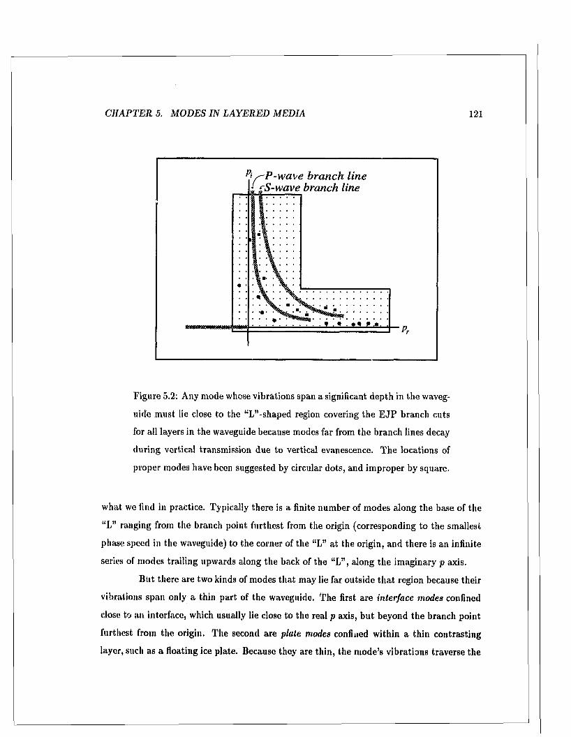
C H A P TE R 5. M O D ES IN L A Y E R E D M ED IA 121
p< s -P -w a v e b ra n ch lin e { fS -w a v e branch line
Figure 5.2: Any mode whose vibrations span a significant depth in the waveg
uide m ust lie close to the “L”-shaped region covering the E JP branch cuts
for all layers in the waveguide because modes far from the branch lines decay
during vertical transmission due to vertical evanescence. T he locations of
proper modes have been suggested by circular dots, and im proper by square.
w hat we find in practice. Typically there is a finite num ber of modes along the base of the
“L” ranging from the branch point furthest from the origin (corresponding to the smallest
phase speed in the waveguide) to the corner of the “L” a t the origin, and there is an infinite
series of modes trailing upwards along the back of the “L” , along the im aginary p axis.
B ut there are two kinds of modes th a t may lie far outside th a t region because their
vibrations span only a thin p art of the waveguide. The first are interface modes confined
close to an interface, which usually lie close to the real p axis, bu t beyond the branch point
furthest from the origin. The second are plate modes confined within a th in contrasting
layer, such as a floating ice plate. Because they are thin, the m ode’s vibrations traverse the
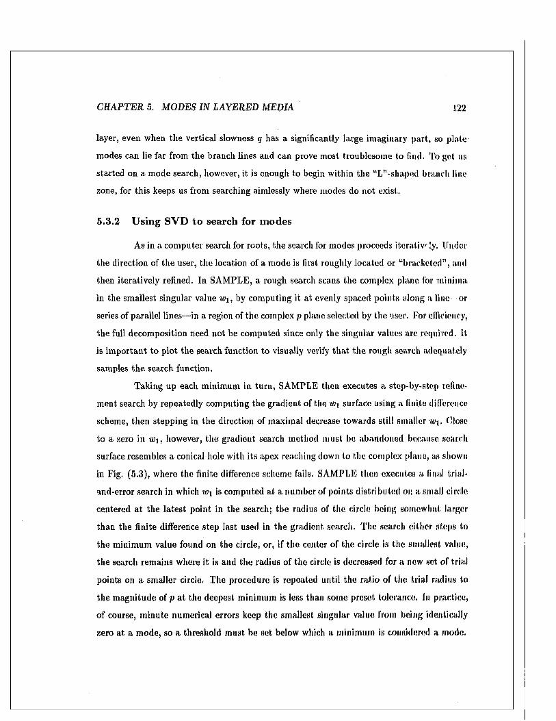
C H A P T E R 5. M O D ES IN L A Y E R E D M ED IA 122
layer, even when the vertical slowness q has a significantly large imaginary part, so plate
modes can lie far from the branch lines and can prove most troublesome to find. To get us
started on a m ode search, however, it is enough to begin within the “L”-shaped branch line
zone, for this keeps us from searching aimlessly where modes do not exist.
5.3.2 U sing SV D to search for m odes
As in a com puter search for roots, the search for modes proceeds iterative !y. Under
the direction of the user, the location of a m ode is first roughly located or “bracketed” , anil
then iteratively refined. In SAM PLE, a rough search scans the complex plane lor minima
in the smallest singular value «q, by computing it at evenly spaced points along a line or
series of parallel lines—in a region of the complex p plane selected by the user. For efficiency,
the full decomposition need not be computed since only the singular values arc required. It
is im portan t to plot the search function to visually verify th a t th e rough search adequately
samples th e search function.
Taking up each minimum in tu rn , SAM PLE then executes a step-by-step refine
m ent search by repeatedly com puting the gradient of the «q surface using a finite difference
scheme, then stepping in the direction of maximal decrease towards still smaller w\. Close
to a zero in «q, however, the gradient search method m ust be abandoned because search
surface resembles a conical hole with its apex reaching down to the complex plane, as shown
in Fig. (5.3), where the finite difference scheme fails. SAM PLE then executes a final trial-
and-error search in which uq is com puted at a number of points d istributed on a small circle
centered a t the la test point in the search; the radius of the circle being somewhat larger
than the finite difference step last used in the gradient search. The search either steps to
the m inimum value found on the circle, or, if the center of the circle is the smallest value,
the search remains where it is and the radius of the circle is decreased for a new set of trial
points on a smaller circle. The procedure is repeated until the ratio of the trial radius to
the m agnitude of p a t the deepest minimum is less than some preset tolerance. In practice,
of course, m inute numerical errors keep the smallest singular value from being identically
zero at a mode, so a threshold m ust be set below which a minimum is considered a mode.
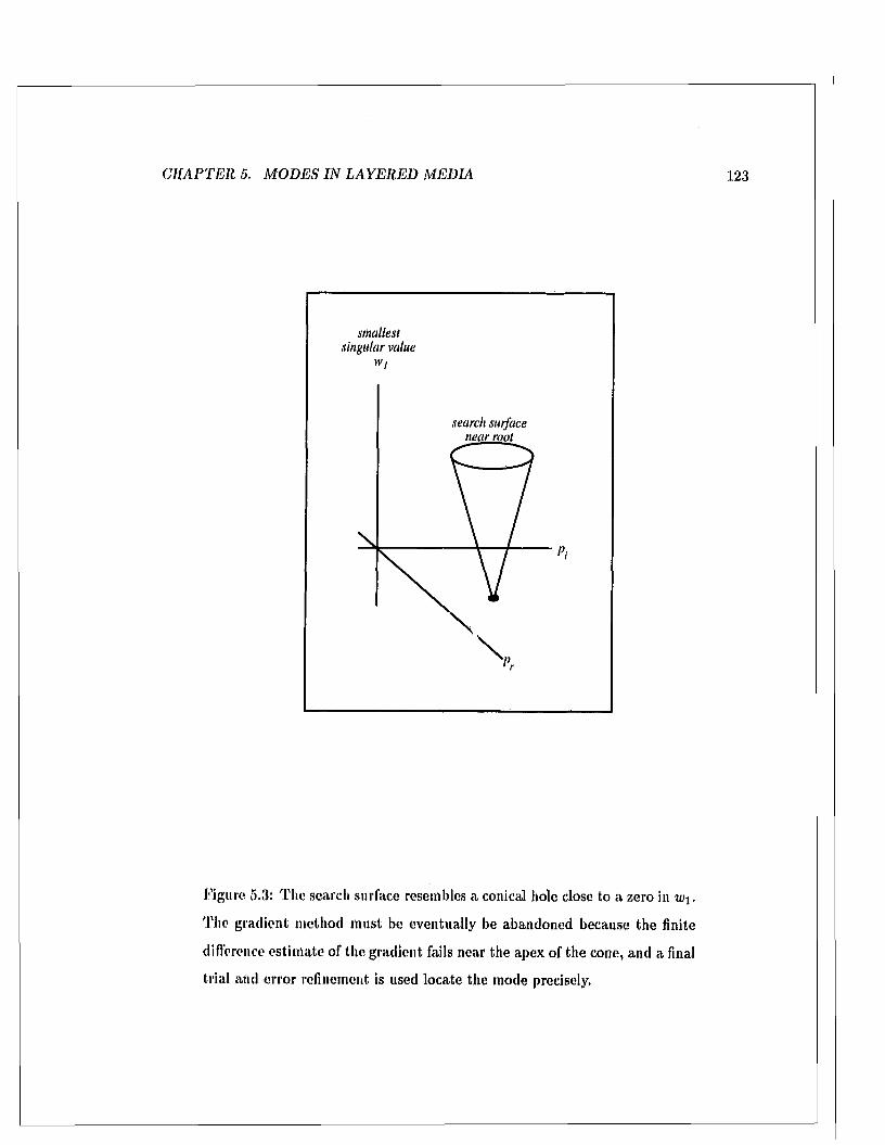
C H A P TER 5. M O D ES IN L A Y E R E D M ED IA 123
smallest singular value
w,
search surface near root
Figure 5.3: The search surface resembles a conical hole close to a zero in W\.
The gradient m ethod m ust be eventually be abandoned because the finite
difference estim ate of the gradient fails near the apex of the cone, and a final
trial and error refinement is used locate the mode precisely.
C H A P T E R 5. M O D ES IN LA YE R E D M ED IA 124
5 .3 .3 W e a k ly c o u p le d c h a n n e ls
One difficulty in the search for roots is the double root or pair of roots uncommonly
close together. These can occur when the waveguide supports two weakly coupled channels
separated by a band of vertically evanescent layers, each having a mode, a t almost the same
slowness p. The theory behind these close mode pairs is the subject of Section (0.5), but for
the mom ent let us consider how to identify and resolve them.
K ennett and Kerry [69] propose splitting the waveguide at a depth between the
weakly coupled channels where their mode functions are numerically zero, The modes in
each channel are then found using two searches, one for each channel separated from tlu*
other, thereby elim inating one mode or the other from each search. Although this channel
separation m ethod works very well as they show, it is difficult to implement in a generally
applicable way, especially for oceanic waveguides where many different channels must be
considered. Moreover, separating the channels disturbs the close mode locations slightly
when their weak coupling is elim inated, and at times it may be their weak interaction tha t
is of particular interest.
W hen using a global or channel m atrix method together with SVI) in the mode
search, we can identify and resolve a double mode or close mode pair using both the smallest
and second smallest singular values, w\ and w^. Two perfectly coincident modes are easily
identified since w\ = wv — 0, in which case the SVD also computes two null-space vectors,
one for each vertical mode function. For a close mode pair, the w\ and w2 surfaces viewed
on a magnified scale look like two inverted cones with their points slightly displaced as
shown in Fig. (5.4). Having refined the location of one mode in the pair using the iterative
method described above, the location of the second can be found by
1. refining the location of a nearby minimum in w? where — wa, point II, starting
from the location of the known mode, point A;
2. c I mating where w\ — 0 by projecting a line through w-i(A) and B to intersect the
complex plane a t point C;
3. refining the second m ode location in w\, s tarting from C with a search resolution
C H A P TE R 5. M O D ES IN L A Y E R E D M ED IA 125
somewhat less than the distance from B to C in the complex plane.
If step I. fails to locate a nearby minimum in w2, there is no close m ode and the procedure is
abandoned. The search program therefore determines when, where, and at what resolution
to search for a nearby mode. An example of a close mode pair is given in Section (6.5).
The question arises whether the m ethod could be used more generally to direct the
search from mode to mode in the complex plane. Unfortunately, the m ethod is unreliable
for widely spaced modes because it relies on linear interpolation. Furtherm ore, the behavior
of w i and w 2 does not generally follow th a t shown in Fig. (5.4) except for close m ode pairs
in weakly coupled channels; there may not always be a m inimum in w 2 between two modes
trapped within the same channel for instance,
5.3.4 Searching for SH m odes
Fluid layers sandwiched between solid layers totally decouple the SH waves prop
agating in the solids. This can be viewe 1 as an extrem e form of layer decoupling peculiar
to SH waves. Using the first and second singular values, each band of consecutive solid
layers can be searched simultaneously for modes, with the fluid layers treated as impene
trable vacuum layers tha t decouple the solid portions of the waveguide while also providing
traction-free boundary conditions for SH waves. In SAM PLE, the user can switch from
P-SV to SH mode com putations using a simple software flag.
5.4 V erifying th e m ode search
At the end of a search we m ust always ask if any significant modes have been
overlooked, or if any found are am iss.8 Several ways to check for missing modes and test
for genuine modes are reviewed below.
"Sometimes a questionable mode inay be found, whose minimum in the search function appears like th a t of a mode, though it does not reach down to the numerical zero of o ther modes. I find these sometimes occur a t slownesses p = 1 /a or 1//? (the branch points) for a layer in the waveguide. W hy they occur is not known. I t is interesting th a t Xie [134] reports similar “false” modes for a floating ice plate found using a different mode search m ethod. B ut they are not always false, p = 1//3 is indeed a m ode for SH waves in a free plate for example.
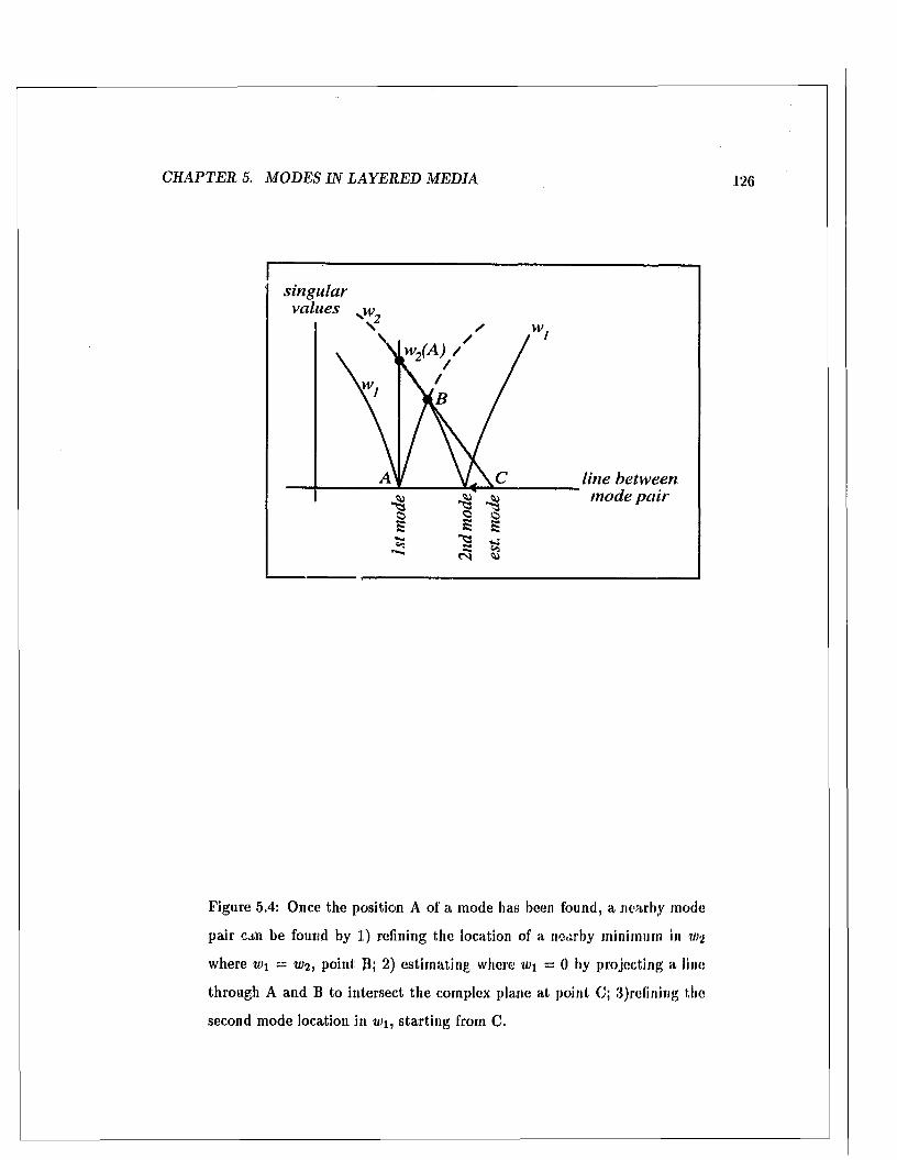
C H A P T E R 5. M O D ES IN L A Y E R E D M ED IA 126
s i n g u l a rv a lu e s
.w
l in e b e t w e e n m o d e p a i r
Figure 5.4: Once the position A of a m ode has been found, a nearby mode
pair can be found by 1) refining the location of a nearby minimum in vi2
where w\ — w2, point B; 2) estim ating where W\ = 0 by projecting a line
through A and B to intersect the complex plane at point C; 3)relining the
second mode location in w\, starting from C.
C H A P TE R 5. M O D ES IN L A Y E R E D M ED IA 127
5.4.1 N ode counting
In the elem entary oceanic waveguide,9 the num ber of nodes (zero crossings) in the
normal stress of each vertical mode function is a way of ordering the modes in a series. A
missing mode can be identified simply by counting the nodes in the m ode functions [66].
Unfortunately, the mode functions for P-SV modes in elastic m edia usually do not follow
this simple ordering scheme because they are made up of a linear com bination of waves
having two vertical slownesses (qa and qp) ra ther than one (qa ). Furtherm ore, the mode
functions—especially for leaky modes—are not real functions of depth as in the elem entary
waveguide, but complex functions produced by inhomogeneous waves, which ruins a direct
relation between the nodes in a mode function and the mode ordering. Nevertheless, node
counting can sometimes be used to detect missing modes in one or another portion of the
mode series. I t works best for propagating duct modes trapped in the w ater column, and
for high order evanescent modes where the regular spacing of modes in the complex plane
tr akes it easy to spot missing modes w ithout node counting.
5.4.2 Contour Integration
The residue theorem shows th a t the contribution of a single m ode to the elastic
field—th a t is, the residue of its pole in the complex plane—m ust be equivalent to a contour
integral encircling ju st th a t mode, and the contribution of m any modes m ust be equivalent
to a contour integral encircling ju st those modes. Thus, it is possible to test p a rt of the
mode series by comparing the resulting field to th a t computed by an encircling contour
integral. The two will be different when a mode is missing or amiss. U nfortunately, a single
test is inconclusive because the contribution of a missing mode m ight be negligibly small for
the source and receiver used to conduct the test, making it impossible to detect its absence.
The test should therefore be repeated using several source and receiver positions.
SAM PLE includes contour integration routines to test modes this way. Space
does not perm it elaboration, except to say th a t an arb itrary contour is specified by the
user using any num ber of straight line segments in the complex plane, and th a t m any
°Sec footnote on page 8.
C H A P T E R 5. M O D ES IN L A Y E R E D M ED IA 128
of the subroutines for contour integration are already available among inode com putation
routines. W hen I added the contour integration routines to SAM PLE, I was not aware of
any other contour integration program th a t computes all components of the elastic field due
to seismic sources in layered elastic media. Dr. Henrik Schmidt has since pointed out to me
tha t Kim [74] wrote such a program in 1989, and th a t it has been included in Dr. Schm idt’s
general purpose seismo-acoustic modeling package called OASES [111]. The main difference
between th e contour integration routines of SAMPLE and those of OASES is tha t SAMPLE
evaluates Hankel integrals of the form (5.2), while OASES evaluates the Bessel integrals of
the form (4.80). T he contour of integration in SAMPLE m ay therefore follow any path in
the complex slowness plane, to verify modes by applying the residue theorem in a flexible,
way, while the contour in OASES (and SAFARI) always runs parallel to the real slowness
axis, to com pute the field due to a point source.
5.4.3 Continuity and boundary conditions
If we are uncertain about a mode, its mode function should be checked to see if it
satisfies all of the boundary and continuity conditions in the waveguide, simply by plotting
the elements of its stress-displacement vector as a function of depth. Only a genuine mode
satisfies all conditions in the waveguide simultaneously.
5.4.4 R ayleigh’s Principle
Takeuchi and Saito [122] recommend verifying a mode using Rayleigh’s Principle,
which states th a t the average kinetic and potential energies are equal for the vertical mode
function. Rayleigh’s Principle is derived in the next section. Using the kinetic and potential
energy term s, u 2 I \ and I? from (5.14) in th a t section, the principle requires th a t w2/-j = /a.
W hen the deviation
c = h i (w2/ i ) - 1 (5.9)
is significantly large it indicates an erroneous mode or mode function. T he test has proven
m ost valuable, and it has been included in SAMPLE.
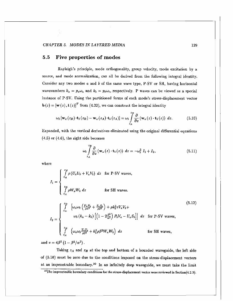
C H A P TE R 5. M O D ES IN L A Y E R E D M ED IA 129
5.5 F ive properties o f m odes
Rayleigh’s principle, mode orthogonality, group velocity, mode excitation by a
source, and mode norm alization, can all be derived from the following integral identity.
Consider any two modes a and b of the same wave type, P-SV or SH, having horizontal
waveriumbers ka = pau a and kb = pt^b, respectively. P waves can be viewed as a special
instance of P-SV. Using the partitioned forms of each m ode’s stress-displacem ent vector
b (z) = [w (z ) , t (z )]r from (4.32), we can construct the integral identity
Zf dUb [wa (zB ) -tb (zB ) - Wa (zA) -tb (zA)] = u b I (wa (z) • t b (z)) dz. (5.10)2.4
Expanded, with the vertical derivatives elim inated using the original differential equations
(4.5) or (4.6), the right side becomes
" d/ Q— (w 0 {z) ■ t 6 («)) dz = - u l I 1 + I 2 ,
where
2/J
1 1 =
f P (UaUb + VaVb) dz for P-SV waves,2/t
2fl
/ pWaWb dz for SH waves.
(5.11)
/2,1h = {
I + + p k 2bWaVb+
u>b (ka - kb) [^1 - 2^ PbVa - Ua5&]] dz for P-SV waves,
7 (“ aU>b + t f p f l 2 W aWb) dzZ A
for SH waves,
(5.12)
and v = 4/?2 (1 - (I2/ a 2) .
Talcing zA and zB a t the top and bottom of a bounded waveguide, the left side
ol (5.10) m ust be zero due to the conditions imposed on the stress-displacem ent vectors
a t an im penetrable boundary .10 In an infinitely deep waveguide, we m ust take the limit
10Tlie im penetrable boundary conditions for the stress-displacem ent vector were reviewed in Section(4.2.3),
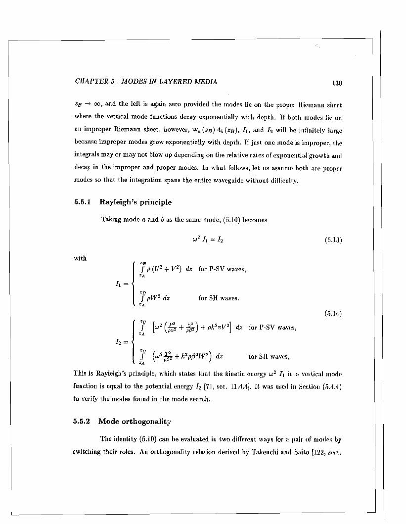
C H A P TE R 5. M O D ES IN L A Y E R E D M ED IA 130
ZB -► oo, and the left is again zero provided the inodes lie on the proper Riemann sheet
where the vertical m ode functions decay exponentially with depth. If both inodes lie on
an im proper R iem ann sheet, however, w, ( zB) -t6 (zB), h , and / 2 will be infinitely large
because im proper modes grow exponentially with depth. If ju st one mode is improper, the
integrals may or m ay not blow up depending on the relative rates of exponential growth and
decay in the im proper and proper modes. In what follows, let us assume both are proper
modes so tha t the integration spans the entire waveguide w ithout difficulty.
5.5.1 R ayleigh’s principle
Taking m ode a and b as the same mode, (5.10) becomes
u 2 h = h (5.13)
with
h =
ZBf p (U2 -f V 2) dz for P-SV waves,
/ pV/ 2 dz for SII waves.
(5.14)
/ [w2 + w ) + p k 2 v V 2} dz for P-SV waves,
h =
/ ( u 2 j ^ + k 2 p/32 W 2) dz for SH waves,Z A
This is Rayleigh’s principle, which states tha t the kinetic energy u 2 /) in a vertical mode
function is equal to the potential energy / 2 [71, sec. 11.4.4]. It was used in Section (5.4.4)
to verify the modes found in the mode search.
5.5.2 M ode orthogonality
The identity (5.10) can be evaluated in two different ways for a pair of modes by
switching their roles. An orthogonality relation derived by Takeuchi and Saito [122, sect.

C H A P T E R 5. M O D ES IN L A YT lE B M ED IA 131
III] follows from the difference of the two,
Z B
(w* - u>1) I x = (kl - k l) f pvVaYb dz for P-SV waves,ZA
( *B ZB+ (ka - kb) U b J tabdz + U a f tbadz
\ Z A ZA
Z B
(u l - w62) h = (kl - k l) f p(32 W aW b dz for SH waves,Z A
where
tab = S bUa - ^1 - 2 ^ j PbVa, (5.16)
and I \ is th a t of (5.12) for the corresponding wave type. This is an orthogonality relation
inasmuch as the right side is zero for any two modes having the same frequency, and the
left is zero for any two modes having the wavenumber.
5.5.3 Group velocity
Group velocity is an im portan t property for the in terpre tation of d a ta from distan t
impulsive sources, for no m atter what shape the initial disturbance has in tim e, it becomes
spread ou t far from the source in a wave train of varying horizontal slowness in which waves
with horizontal wavenumber k = u p move at a velocity roughly equal to the group velocity
ca (k) = du> (k) / d k [113, sect. 9.3]. The group velocity for a mode can be approxim ately
evaluated by changing its frequency slightly while tracking the m ode along its dispersion
curve.11 Proceeding this way, we can again apply (5.10) in two different ways, first with
u a = w, u>b = w + 6 w, k a = k = up , and kb = k -f 6 k, and then with Ub = u , u a = u + Su,
kb - k, and ka = k -f 6 k. Taking the difference between the identities, retaining term s to
first order, gives
0 = - 2 u ( i i 6 u - p l 3 6 k ) , (5.17)
11A dispersion curve is a plot of the horizontal slowness, wavenumber, phase speed, or group velocity of a mode as frequency ui is varied continuously. A mode whose phase speed is independent of u is non-dispersive.
(5.15)
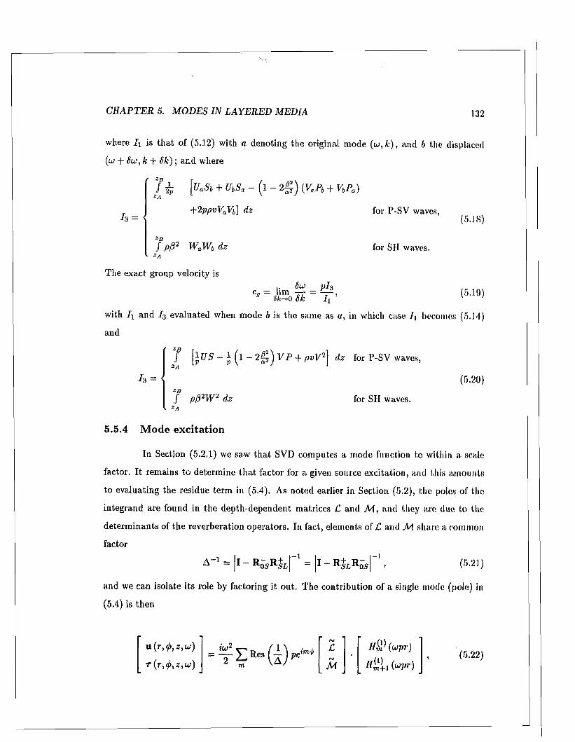
C H A P T E R 5. M O D ES IN L A Y E R E D M ED IA 132
where i i is th a t of (5.12) with a denoting the original mode (w, k ) , and b the displaced
(a; + 6 u , k + 6 k ) ; and where
ZBf
ZA+2ppvVaVb] dz
h =
7 TP [U^ b + UbS a - ( l - 2 g ) (VaPb + VbPa)
ZBf p/32 W aW b dz
The exact group velocity is
for P-SV waves,
for SII waves.
(5.18)
6 u> p f 3 c„ — lim — = — .
Sk->o 6 k L ' (5.19)
with I i and I 3 evaluated when mode b is the same as «, in which case /, becomes (5. 1/ 1)
and
h =
7 [ l U S - l ( l - 2 ^ ) V P + p v V 2\ dz for P-SV waves,Z A
(5.20)ZBJ p/32 W 2 dz
ZA
5.5.4 M ode excitation
for SI1 waves.
In Section (5.2.1) we saw th a t SVD computes a mode function to within a scale
factor. I t remains to determ ine th a t factor for a given source excitation, and this am ounts
to evaluating the residue term in (5.4). As noted earlier in Section (5.2), the poles of the
integrand are found in the depth-dependent m atrices C and M , and they are due to the
determ inants of the reverberation operators. In fact, elements of C and M share a common
factor
I R q s R ^ l - I - R-s/.R-o.v- i
(5.21)
and we can isolate its role by factoring it out. The contribution of a single mode (pole) in
(5.4) is then
t u ‘~ 2
rvC IIv ? ( w p r )fS*
M _ 11 m+ l (W|W) _(5.22)
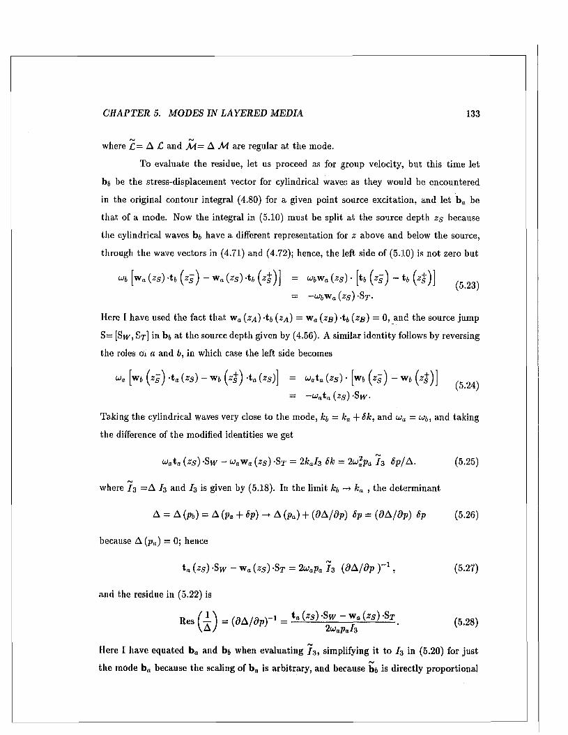
C H A P TE R 5. M O D ES IN L A Y E R E D M ED IA 133
r>j is,4
where C — A C and M = A M are regular at the mode.
To evaluate the residue, let us proceed as for group velocity, bu t this tim e let
b;, be the stress-displacement vector for cylindrical waves as they would be encountered
in the original contour integral (4.80) for a given point source excitation, and let b 0 be
tha t of a mode. Now the integral in (5.10) m ust be split a t the source depth z s because
the cylindrical waves b 4 have a different representation for z above and below the source,
through the wave vectors in (4.71) and (4.72); hence, the left side of (5.10) is not zero but
Wfc [w„ (zS) t b ( Z s ) - w a (zs ) -tfc ( 4 )] = UbWa (zS ) ■ [t6 ( % ) - t 6 (4 )]
= - c j b'wa (zs )-ST.
Here I have used the fact th a t w a (24) -tb (z a ) = w a (zg ) -tb (zg ) = 0, and the source jum p
S= [Sw, S t] in b 4 a t the source depth given by (4.56). A similar identity follows by reversing
the roles oi a and b, in which case the left side becomes
W„ [wfc (4 ) -ta (Zs) ~ W6 ( 4 ) '*0 (*s)] = Wat a (zS ) • [w4 (zg ) - Wfc (4 )] , ,(5.24j
= -w at a (zs) -Svv-
Ta.king the cylindrical waves very close to the mode, kb = ka + Sk, and uia = u b, and taking
the difference of the modified identities we get
Wat a (z s ) -Svv - waw a (zs ) -ST = 2kaI 3 Sk = 2LJ%Pa I 3 t ip /A. (5.25)
ISJwhere /3 = A I 3 and I 3 is given by (5.18). In the lim it kb ka , the determ inant
A = A (pb) = A (pa + Sp) -+ A (pa) + ( d A / d p ) Sp = ( d A / d p ) Sp (5.26)
because A (pa) = 0; hence
ta (zs) -Sw - Wa (zs ) -S t = 2u apa I 3 ( d A / d p )_ 1 , (5.27)
and the residue in (5.22) is
Res ( 1 ) = ( d b / O p ) - ' = (5 28)
Here I have equated ba and b4 when evaluating 73, simplifying it to I3 in (5.20) for just
the mode b„ because the scaling of bn is arbitrary , and because b4 is directly proportional
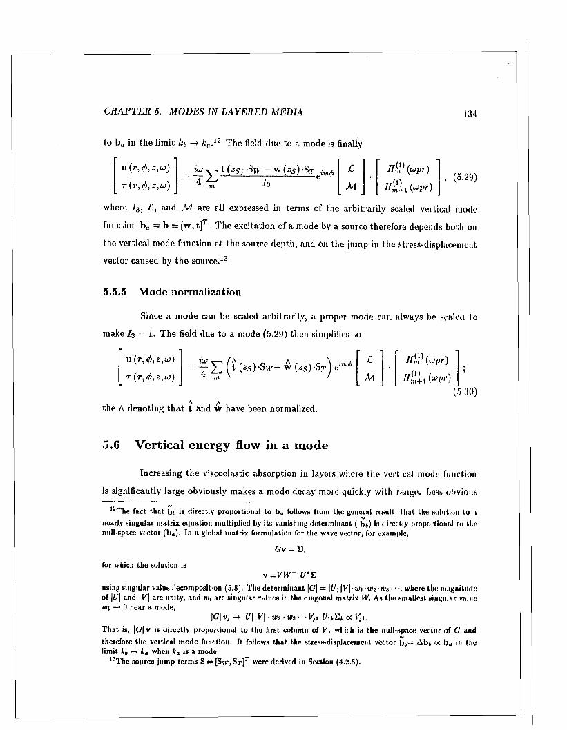
C H A P T E R 5. M O D ES IN L A Y E R E D M ED IA 134
to b 0 in the lim it kb —> fca.12 The field due to a mode is finally
U (r,<f>,z,u) _ i u t (zs , -SMr - w (zs) -S t j mih jC 1 1 $ (uipr)
T(r,<f>,z,u) 4 ^ I3m J M H m l i ( w r ) _, (5.29)
M J ILnU ^> >r) _
where / 3, £ , and Af are all expressed in term s of the arbitrarily scaled vertical mode
function b a = b = [w ,t]T . T he excitation of a mode by a. source therefore depends both on
the vertical mode function a t the source depth, and on the jum p in the stress-displacement
vector caused by th e source.13
5 .5 .5 M o d e n o r m a l i z a t i o n
Since a m ode can be scaled arbitrarily, a proper mode can always be scaled to
make / 3 = 1. The field due to a mode (5.29) then simplifies to
u (r,^>,z,u)
r(r,<j>,z,u)= T X) (* (zs) •Sh'- w (25) -St )
C
M
11$ (wpr)
IrvX\(5.30)
the A denoting th a t t and w have been normalized.
5.6 V ertical energy flow in a m ode
Increasing the viscoelastic absorption in layers where the vertical mode function
is significantly large obviously makes a mode decay more quickly with range. Less obvious
12The fact th a t b s is directly proportional to b„ follows from the general result, th a t the solution to a1 • . • . I’v
nearly singular m atrix equation m ultiplied by its vanishing determ inant ( bi,) is directly proportional to the null-space vector (b a). In a global m atrix formulation for the wave vector, for example,
G v = E ,
for which the solution isv z z V W - ' U ’ E
using singular value Jecom posit.on (5.8). The determ inant \G\ = \U\ |Vj-u/i • 1112 • 1113 • < •, where the m agnitude of \U\ and |Vj are unity, and ui; are singular "allies in the diagonal m atrix W, As the sm allest singular value v>\ -* 0 near a mode,
|G| v, -> \U\\V\ ■ w 2 . w3 • • • Vj, UikZk oc VJt .
T h a t is, |C7| v is directly proportional to the first column of V, which is the null-space vector of (J and
therefore th e vertical m ode function. I t follows th a t the stress-displacem ent vector b s = Abi, oc b« in the lim it kb —* k a when ka is a mode,
13The source jum p term s S = [Siv, St ]7" were derived in Section (4,2.5).
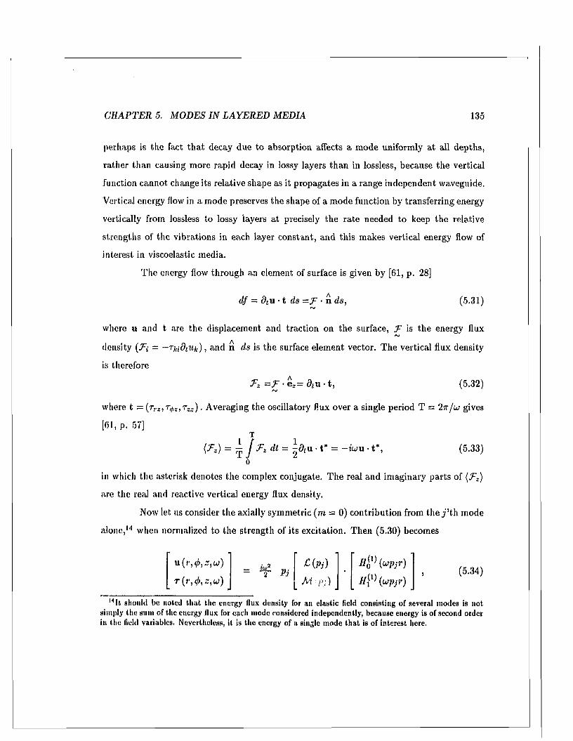
C H A P T E R 5. M O D ES IN L A Y E R E D M ED IA 135
perhaps is the fact th a t decay due to absorption affects a m ode uniformly a t all depths,
rather than causing more rapid decay in lossy layers than in lossless, because the vertical
function cannot change its relative shape as it propagates in a range independent waveguide.
Vertical energy flow in a m ode preserves the shape of a m ode function by transferring energy
vertically from lossless to lossy layers a t precisely the ra te needed to keep the relative
strengths of the vibrations in each layer constant, and this makes vertical energy flow of
interest in viscoelastic media.
The energy flow through an element of surface is given by [61, p. 28]
df = dtu • t ds —T • n ds, (5.31)
where u and t are the displacement and traction on the surface, T is the energy flux/Ni
density {!Fi — - TkidiUk) , and n ds is the surface element vector. The vertical flux density
is therefore
Fz = T • e z= dtu • t , (5.32)
where t = ( r r z , t$z , tz z ) . Averaging the oscillatory flux over a single period T = 2 tt/ uj gives
[61, p. 57]
(Fz) = ^ J Fz (It - i dtu • t* = - tu rn • t*, (5.33)
in which the asterisk denotes the complex conjugate. The real and im aginary parts of (jFz)
are the real and reactive vertical energy flux density.
Now let us consider the axially symmetric (m = 0) contribution from the j ’th mode
alone,1,1 when normalized to the strength of its excitation. Then (5.30) becomes
(5.34)u (r,</>, 2 , w) iufi £ (P j ) H ^ i u p j r )
r ( r ,<l> , z ,u>)= - f - Pj
M ; / 1;) _ n [ 1 ] ^ P j r ) _H U should be noted th a t the energy llux density for an elastic field consisting of several inodes is not
simply the sum of the energy flux for each mode considered independently, because energy is of second order in the field variables. Nevertheless, it is the energy of a single mode th a t is of interest here.
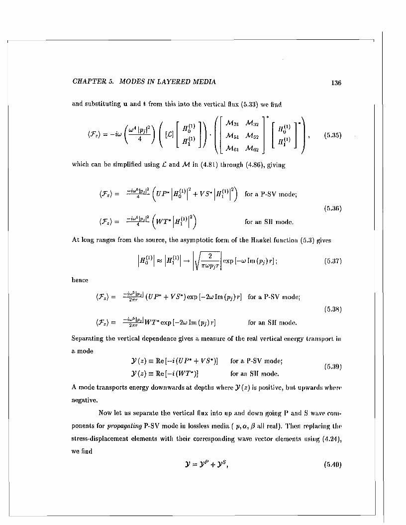
C H A P T E R 5. M O D E S I N L A Y E R E D MEDIA 136
and substitu ting u and t, from this into the vertical flux (5.33) we find
(F. ) = - iu ; ( [C]
Ad31 Ada2
A fs i A f 52
Ad 61 Ad 62
/ / ( ' ) n o
//{»(5.35)
which can be simplified using C and Ad in (4.8") " ough (4.86), giving
( F g ) = ( u p *\h W\ + VS* for a P-SV mode;
( K ) =p i (
(5.36)
W T * H P for an SH mode.
A t long ranges from the source, the asym ptotic form of the Hankel function (5.3) gives
| 4 ° | « |//i(1) irujpjrexp [-u> Im {pj) r}; (5.37)
hence
<^> =5 jp, |
2 -kt (UP* -f- ViS'^exp [-2 w lm (p j)r] for a P-SV mode;
(5.38)
(A-) = exp [ - 2w Im (pj) r] for an SH mode.
(5.39)
Separating the vertical dependence gives a measure of the real vertical energy transport in
a modey (z) = Re [ - i (UP* + V S *)] for a P-SV mode;
y (z) = Re H (WT*)] for an SH mode.
A mode transports energy downwards at depths where y(z) is positive, but upwards when*
negative.
Now let us separate the vertical flux into up and down going P and S wave com
ponents for propagating P-SV mode in lossless media ( p ,a , [i all real). Then replacing the
stress-displacement elements with their corresponding wave vector elements using (4.24),
we find
y = yp + ys, m o )
^
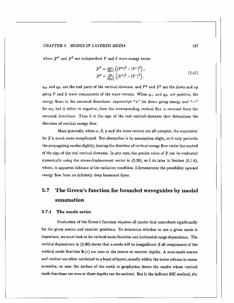
C H A P TER 5. M O D ES IN L A Y E R E D M ED IA 137
where y p and y s are independent P and S wave energy terms
= * i ( i ^ i 2 - if - l 2) • .....^ * (|s+la - l* '|a) •
(jar and qpT are the real parts of the vertical slowness, and P ± and S± are the down and up
going P and S wave components of the wave vectors. W hen qnr and qpr are positive, the
energy flows in the assum ed directions: superscript for down going energy and “— ”
for up; but if either is negative, then the corresponding vertical flux is reversed from the
assumed directions. Thus it is the sign of the real vertical slowness th a t determines the
direction of vertical energy flow.
More generally, when a , /?, p and the wave vectors are all complex, the expression
for y is much more complicated. B u t absorption is by assum ption slight, so it only perturbs
the propagating modes slightly, leaving the direction of vertical energy flow under the control
of the sign of the real vertical slowness. In any case, the precise value of y can be evaluated
numerically using the stress-displacement vector in (5.39), as I do la te r in Section (6.1.4),
where, in apparent defiance of the radiation condition, I dem onstrate the possibility upward
energy flow from an infinitely deep basement layer.
5.7 T h e G reen ’s function for bounded w aveguides by m odal
sum m ation
5.7.1 The m ode series
Evaluation of the Green’s function requires all modes th a t contribute significantly
for the given source and receiver positions. To determ ine whether or not a given mode is
im portant, we m ust look at its vertical mode function and horizontal range dependence. The
vertical dependence in (5.30) shows th a t a m ode will be insignificant if all com ponents of the
vertical mode function b ( s ) are zero a t the source or receiver depths. A m an-m ade source
and receiver are often restricted to a band of layers, usually within the w ater column in ocean
acoustics, or near the surface of the earth in geophysics; hence the modes whose vertical
inode functions are zero a t those depths can be om itted. B ut in the indirect B IE m ethod, the
C H A P T E R 5. M O D ES IN L A Y E R E D M ED IA 138
source and receiver locations vary freely, including nodes on the boundary of tlie inclusion,
the location of sources generating the particular solutions, and the com putation points for
the whole-, surface-, and null-held equations; so more modes are generally required. The
range dependence of a mode shows th a t a mode will be insignificant if the Hankel function
becomes very small. W ith physical sources, we m ust specify a lower limit on the distance
between the source and receiver 7 'm i n because a real source is not point-like in its near-field.
In the B IE m ethod, we also m ust specify a minimum range for the ideal point source
for numerical reasons. The Hankel functions in each mode are singular at r = 0, which
makes the terms in the mode series very large term s, and the sum becomes lost, in extreme
cancellation.
T he lower bound r mj„ fixes an upper bound in the complex slowness plane above
which modes cannot contribute significantly. As p in a mode series moves upwards term
by term in the complex slowness plane, the argum ent of the liankel function eventually
satisfies u p , r > 1, and the exponential asym ptotic form of the liankel function (5.3) can
be used, which decays exponentially with further increases in the. im aginary slowness p, ,
Hence, we can safely assume th a t the significant modes lie below the value of p, at which
the exponential envelope of the Hankel functions reaches some small value o,
e > |e*u'pr| = \ e - ^ ' T\ with 0 < c < 1, (5.-12)
which implies, , — In«r ^ - I n c ,r
P i ( r ) < ------< _ _ _ . (5/13u r w r m j„
This fixes an upper bound on the “L”-shaped region of Fig. (5.2) lor any range. When
vmin for a particular application is large, as it is for long range propagation modeling, all
of the im portan t modes m ust lie close to the real p axis. B ut when r,,,;,, is small, the mode
series, and therefore the mode search, m ust venture far from the real p axis, In the indirect
BIE m ethod, 7‘min should be slightly smaller than the radius of the close neighborhood
of a com putation point, within which a boundary element is autom atically designated as
troublesome, to ensure th a t all of the significant modes are available.
C H A P T E R 5. M O D ES IN L A Y E R E D M ED IA 139
5.7.2 Series convergence
The sum of a long series of complicated terms can be com puted more quickly if
the term s are first ordered from largest to smallest, for then we can tes t convergence as
the sum m ation progresses, p< jsibly by checking if the la test terms edded are negligibly
small compared with the latest partial sum, to halt the series w ithout adding all of its
insignificant terms. A good way of ordering modes is to sort them from smallest to largest
im aginary slowness because, in a long series of evanescent modes, the m agnitude of the
terms eventually follows the exponential decay of the asym ptotic Hankel function, making
it likely th a t successive terms will on the whole be steadily decreasing. I t is best to decide
when a mode series has converged by testing only the exponential decay envelope of the
Hankel function using (5.43), ra ther than testing the relative size of the latest term in the
series, There are two reasons for this. When computing the entire G reen’s displacement
and stress tensors due to a point source, there are a to tal of 27 unique field variables
(three displacement and six stress for each of three Cartesian axes) th a t m ust be tested
to assure convergence, making the convergence test itself a weighty burden, against which
(5.42) appears trivial. More im portantly, the vertical dependence of inodes can m ake the
contributions of a few sequential modes negligibly small, thereby fooling the convergence
test to stop the series prematurely. False convergence tests can be reduced by requiring th a t
a num ber of successive convergence tests have passed successfully, but the scheme would
not be foolproof.
5.7.3 The G reen’s function singularity
For the G reen’s function to satisfy the equation of m otion (2.50), it m ust have a
waveguide, this singularity arises from the infinite mode series, in p art because of the
singularity in the Hankel function range dependence of each series
singularity in order th a t its spatial gradient produces a 5-function behavior. In a bounded
Hni //q 1* (upr) = j Jim In (a>pr) = -o o ;(5.44)
m > 0
C H A P T E R 5. M O D ES IN L A Y E R E D M ED IA 140
(the H singularity contributing a delta-function behavior <5 (r) /?•), and in part because
of lack of convergence in the infinite series of evanescent modes trailing upwards along the
im aginary p axis (contributing 6 (z - zs )). The infinite series of modes work to cancel out
the Hankel function singularities of all modes along the vertical line through the source,
v.iiile also shaping the delta-function singularity at the source depth. At very short ranges,
then, the mode series for a point source becomes one of infinitely large terms whose mutual
cancellation lose the finite sum in numerical error. The problem occurs a t small horizontal
ranges, regardless of the vertical separation of source and receiver, because the term s in
the m ode series are infinitely large. This is why we must place a lower bound r„,in on the
range between source and receiver in (5.43), and why we encounter convergence problems
in the B IE m ethod for layered m edia whenever the com putation point lies directly above
or below the scattering inclusion.
Convergence problems of one sort or another always seem to plague near-field
Green’s function evaluations for layered m edia no m atter what m ethod is used. In un
bounded waveguides, the branch line integrals face similar convergence problems because
their integrands behave roughly like the evanescent mode series. Alternatively, the contour
integrals (4.80) along the positive real p axis could be evaluated directly, with the range
dependence in the integrands kept in terms of Bessel functions Jin (uipr) , which are well-
behaved as r —> 0. No doubt avoiding the Hankel function singularities this way helps
in the near field, bu t convergence problems still occur close to the source point due to
oscillatory integrands, much as Gerstofi, and Schmidt [50] report in their two-dimensional
BIE m ethod .15 It m ay be advantageous to switch from a modal to such a contour integral
representation, depending on the proxim ity to the source and receiver, as Lu and Kelson
do in their hybrid ray-m ode model [84] [85]. I do not explore the possibility here, but rely
instead on the indirect BIE method to avoid the very near field altogether.
15To accelerate convergence of the slowly decaying oscillatory integrand for points the near field, (Jcr- stoft and Schm idt force the integrands to zero artificially by multiplying them by a gradual monotonieally decreasing function of k = up.
C H A P TE R 5. M O D ES IN L A Y E R E D M ED IA 141
5.8 M odel verification
1 have charted a ra ther long course to develop the channel m atrix m ethod for
normal modes to com pute the field due to a point source in layered media. To dem onstrate
that it is practicable, I will compare the SAM PLE program based upon it with the well-
known and well-established SAFARI program (version 4.0) [109]. An exhaustive verification
this way is not possible because SAFARI only supports axially sym m etric sources (uniform
explosive and vertical point source), only computes t z z , u r , u z ] and is not accurate at
small ranges r < \ a . SAM PLE is equipped with Fast Fourier Transform (F F T ) contour
integration routines like those of SAFARI, but they are based upon the channel m atrix
m ethod ra ther than the global m atrix m ethod of SAFARI. These will also be reported .10
5.8.1 Arctic ocean m odel
A shallow Arctic ocean sound speed profile is given in Table (5.1). The waveguide
has a 3 m ice layer a t the surface, a 200 m w ater column typical of the A rctic ocean [66] [130],
two 2 m sediment layers at the sea floor, and 2000 m deep rock basement layer bounded
below by an im penetrable rigid boundary. The field due a 20 Hz dilatational point source
at a depth of 10 m and a, vertical point source at the ice surface will be computed.
Let us begin with the search for modes closest to the real horizontal slowness axis.
Fig. (5.5) shows the smallest and second smallest singular values, w\ and W2 , along the
axis, wi is the search function whose m inim a suggest the presence of modes close to the
axis. M ode locations were refined from these, and from other m inim a detected in the same
way in searches along the P and S wave branch lines for the deep basement layer.17 Fig.
(5.6) shows the modes in the complex slowness plane on a scale so expanded th a t the lowest
order plate mode (m ode 1) has been forced off the diagram. Fig. (5.7) shows the vertical
mode functions for the first 5 modes ordered by descending pr . There are o ther modes,
such as evanescent modes needed in the very near field, and modes trapped in the two
,sMore extensive testing of all components in the elastic field could be done using the OASES m od e l[lll] , which is much more com plete than SAFARI (see page 15). I did not use OASES here because it is a very recent program, and I was unaware of its capabilities until very late in my project,
17Thc reason for searching along the branch lines for the basem ent layer in a bounded waveguide is th a t radiation tnodcn are found nearby; see Section (6.4).
C H A P T E R 5. M O D ES IN L A Y E R E D M ED IA 142
sediment layers, th a t have not been included in the search because they will not contribute
significantly in these tests.
Now let us consider the SAM PLE and SAFARI contour integration models. When
using a contour integration routine, it is recommend to plot the integrand for the desired
field variable to ensure adequate sampling. Fig. (5.8) shows the magnitude of the vertical
dependence in the integrand for tzz com puted by SAFARI (dotted) and SAM PLE (dashed)
at a depth of 10 m for the d ilatational point source a t depth 10 m. In both cases the contour
was displaced slightly below the positive re d slowness axis to avoid crossing directly over
the poles due to modes. As it is, the sharp peaks indicate where the contour passes over
the shoulder of a nearby pole due to a mode. The models differ by a constant scaling factor
because SAFARI normalizes the field to its strength at one m eter from the source, whereas
SAMPLE uses the absolute strengths given to the source. The factor has been removed
by normalizing each curve to its m axim um value. Close agreement between the two curves
makes them indistinguishable. Imposed upon Fig. (5.8) are the relative contributions of
the dom inant modes at a d istan t receiver. There is one mode at the horizontal slowness of
every sharp peak in the contour due to the connection between modes and peaks. Perfect
agreement between the peak heights and mode strengths should not be expected because
m ultiplication by Hankel-function range dependence and integration over slowness transform
the contour peaks in to mode contributions. Fig. (5.9) shows the normal stress field plotted
as a function of horizontal distance from the source. The three results are indistinguishable
in the figure.
Fig. (5.10) shows the vertical displacement due to a vertical point force acting at
the surface of the ice com puted by all three models.
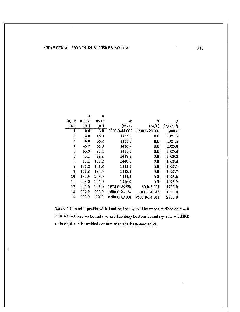
C H A P T E R 5. M O D ES IN L A Y E R E D M ED IA 143
z ziyer upper lower a (3 Pno. (m) (m) (m /s) (m /s) (k g /m 3)
1 0.0 3.0 3300.0-33.00i 1730.0-20.00i 900.02 3.0 16.0 1436.3 0.0 1024.53 16.0 38.2 1436.3 0.0 1024.54 38.2 55.9 1436.7 0.0 1025.05 55.9 75.1 1438.3 0.0 1025.66 75.1 92.1 1439.9 0.0 1026.37 92.1 135.2 1440.6 0.0 1026.68 135.2 161.8 1441.5 0.0 1027.19 161.8 180.5 1443.2 0.0 1027.7
10 180.5 203.0 1444.3 0.0 1028.011 203.0 205.0 1446.0 0.0 1028.212 205.0 207.0 1575.0-28.86i 80.0-2.20i 1700.013 207.0 209.0 1650.0-24.18i 110.0 - 5.04i 1900.014 209.0 2209 5250.0-19.00i 2500.0-18.00i 2700.0
Table 5.1: Arctic profile with floating ice layer. The upper surface a t z = 0
m is a traction-free boundary, and the deep bottom boundary a t z = 2209.0
in is rigid and in welded contact with the basement solid.
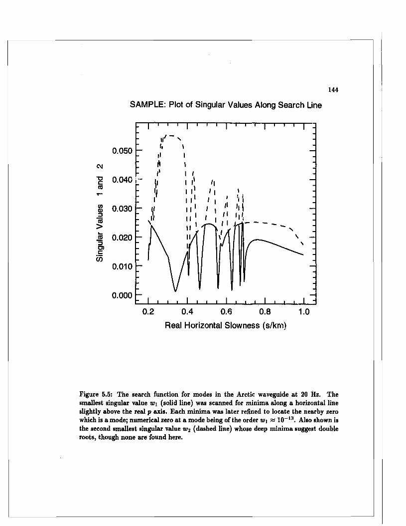
144
SAMPLE: Plot of Singular Values Along Search Line
./ —
0.050
■o 0.040 <0
% 0.0303(0>
0.020
0.010
0 .0 0 0
0.40.2 0.6 0.8 1.0Real Horizontal Slowness (s/km)
Figure 5.5: The search function for modes in the Arctic waveguide at 20 Hz. The smallest singular value Wi (solid line) was scanned for minima along a horizontal line slightly above the real p axis. Each minima was later refined to locate the nearby zero which is a mode; numerical zero at a mode being of the order W j « 10“ i:*. Also shown is the second smallest singular value W2 (dashed line) whose deep minima suggest double roots, though none are found here.
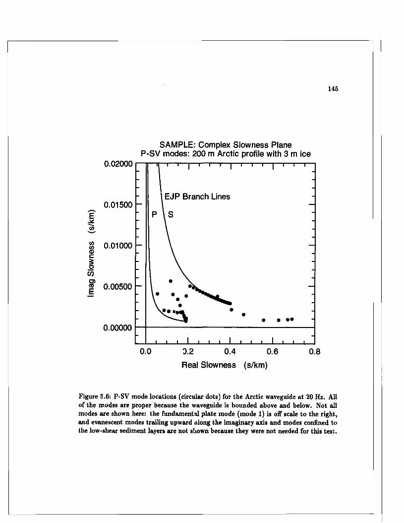
145
SAMPLE: Complex Slowness PlaneP-SV modes: 200 m Arctic profile with 3 m ice
0.02000-
— rr i".. t | i i i | i i i— f— i— i— r
: l EJP Branch Lines0.01500 — 1 —
I f- P \ s- \- \
V> 0.01000 — \ _I(DC“ - \Up5 -o
CO m \
f 0.00500 —• \
—c -
_
V •-• • • •
0.00000-
■ i i 1 i i i 1 i i i 1 i i i0.0 0.2 0.4 0.6 0.8
Real Slowness (s/km)
Figure 5.6: P-SV mode locations (circular dots) for the Arctic waveguide at 20 Hz. Allof the modes are proper because the waveguide is bounded above and below. Not allmodes are shown here: the fundamental plate mode (mode 1) is off scale to the right,and evanescent modes trailing upward along the imaginary axis and modes confined tothe low-shear sediment layers are not shown because they were not needed for this test.
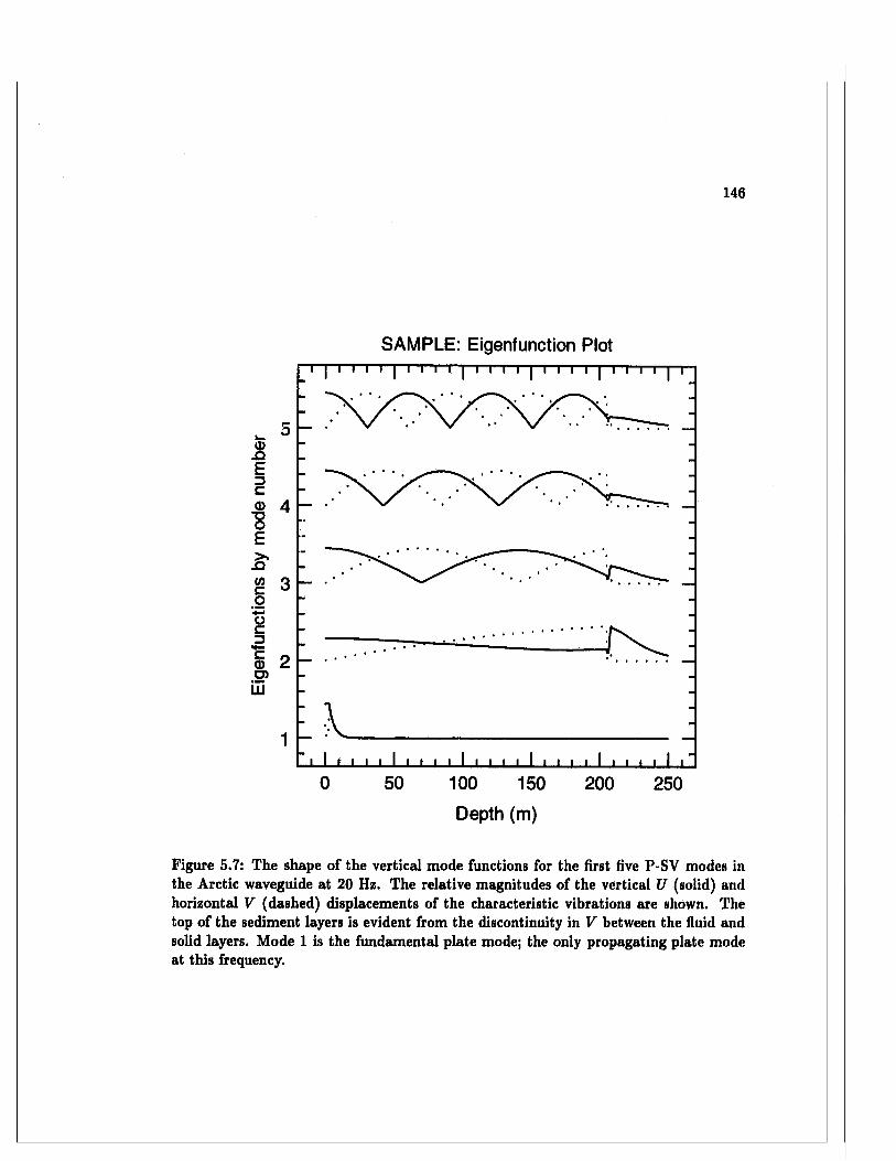
146
SAMPLE: Eigenfunction Plot
<i>X)EDCd>SE£(0co'■*-*ocDcd)o>iH
5
4
3
2
1
0 50 100 150 200 250Depth (m)
Figure 5.7: The shape of the vertical mode functions for the first five P-SV modes in the Arctic waveguide at 20 Hz. The relative magnitudes of the vertical U (solid) and horizontal V (dashed) displacements of the characteristic vibrations are shown. The top of the sediment layers is evident from the discontinuity in V between the fluid and solid layers. Mode 1 is the fundamental plate mode; the only propagating plate mode at this frequency.
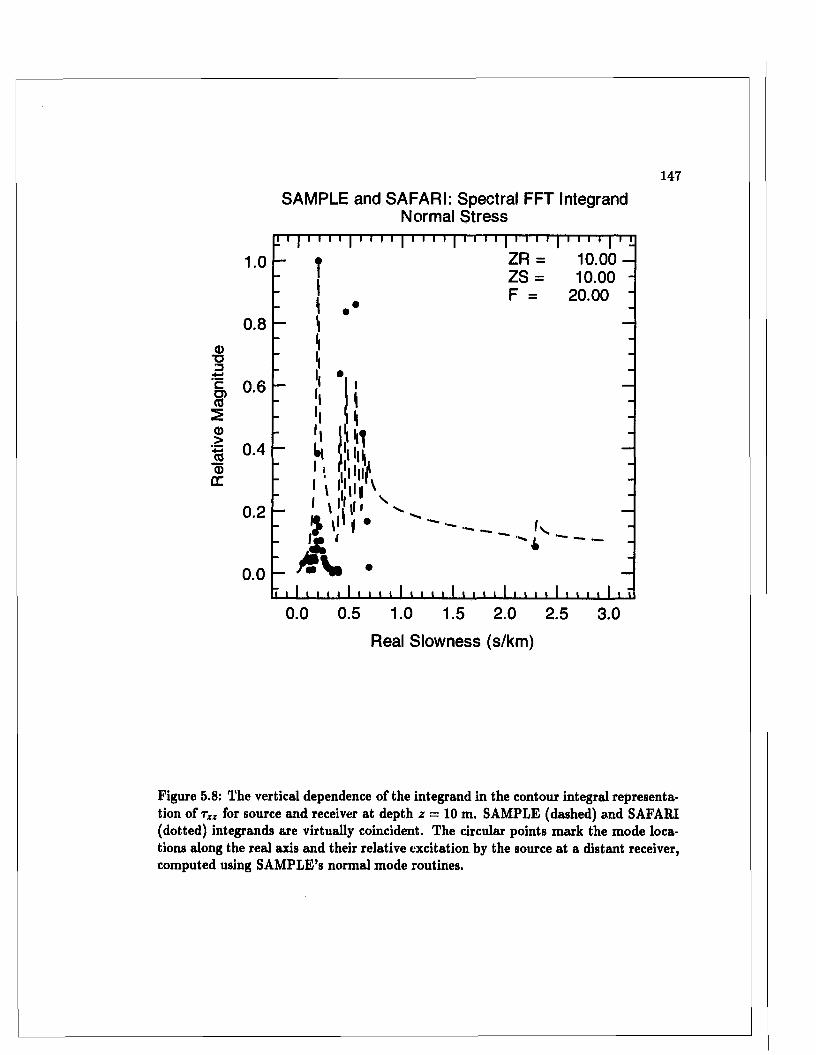
147
SAMPLE and SAFARI: Spectral FFT Integrand Normal Stress
ZR = 10.00 -Z S = 10.00 -F = 20.00 "
0.8
c 0.6o> ^co2(D
I 0 .4Q)DC
0.2
0.0
0.0 0.5 1.0 1.5 2.0 2.5 3.0
Real Slowness (s/km)
Figure 5.8: The vertical dependence of the integrand in the contour integral representation of tZ2 for source and receiver at depth z = 10 m. SAMPLE (dashed) and SAFARI (dotted) integrands are virtually coincident. The circular points mark the mode locations along the real axis and their relative excitation by the source at a distant receiver, computed using SAMPLE’S normal mode routines.
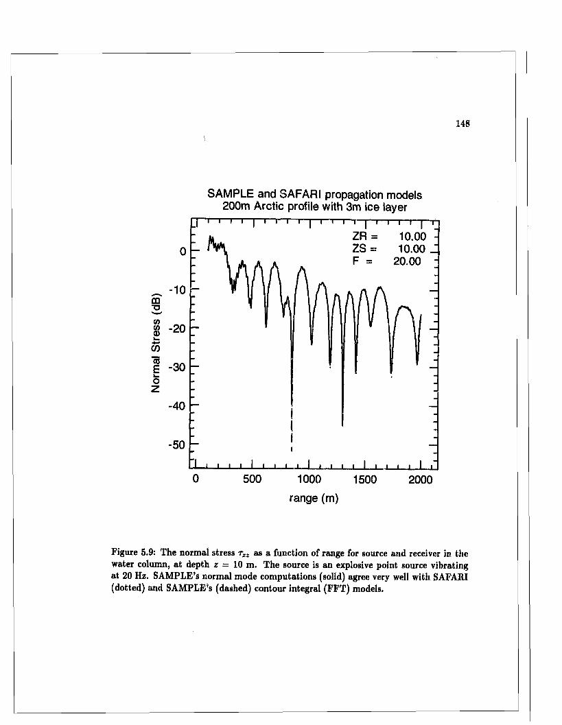
SAMPLE and SAFARI propagation models 200m Arctic profile with 3m ice layer
ZR = 10.00ZS = 10.00F = 20.00
-10CQ■O
CO
E -30oZ
-40
-50
0 500 1000 1500 2000
range (m)
Figure 5.9: The normal stress rzz as a function of range for source and receiver in the water column, at depth z = 10 m. The source is an explosive point source vibrating at 20 Hz. SAMPLE’S normal mode computations (solid) agree very well with SAFARI (dotted) and SAMPLE’S (dashed) contour integral (FFT) models.
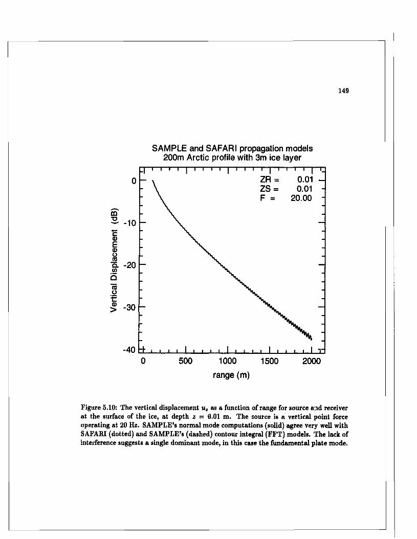
149
SAMPLE and SAFARI propagation models 200m Arctic profile with 3m ice layer
ZR = 0.01ZS = 0.01F = 20.00
CD
s -10c®E<33O(0o. -20Cfl
Q«ok.
-400 500 1000 1500 2000
range (m)
Figure 5.10: The vertical displacement uz as a function of range for source and receiver at the surface of the ice, at depth z — 0.01 m. The source is a vertical point force operating at 20 Hz. SAMPLE’S normal mode computations (solid) agree very well with SAFARI (dotted) and SAMPLE’S (dashed) contour integral (FFT) models. The lack of interference suggests a single dominant mode, in this case the fundamental plate mode.
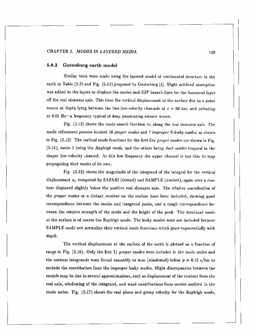
C H A P T E R 5. M OD ES IN L A Y E R E D M ED IA 150
5.8.2 Gutenburg earth m odel
Similar tests were made using the layered model of continental structure in the
earth in Table (5.2) and Fig. (5.11) proposed by G utenburg [1]. Slight artificial absorption
was added to the layers to displace the modes and E JP branch lines for the basement layer
off the real slowness axis. This time the vertical displacement at the surface due to a point
source a t depth lying between the two low-velocity channels at 2 = 50 km, and pulsating
at 0.05 Hz—a frequency typical of deep penetrating seismic waves.
Fig. (5.12) shows the mode search function W\ along the real slowness axis. The
mode refinement process located 16 proper modes and 7 improper S-leaky modes, as shown
in Fig. (5.13) T he vertical mode functions for the first five proper modes are shown in Fig.
(5.14); mode 1 being the Rayleigh mode, and the others being duet modes trapped in the
deeper low-velocity channel. At this low frequency the upper channel is too thin to trap
propagating duct modes of its own.
Fig. (5.15) shows the m agnitude of the integrand of the integral for the vertical
displacement uz com puted by SAFARI (dotted) and SAMPLE (dashed), again over a con
tour displaced slightly below the positive real slowness axis. T he relative contribution of
the proper modes a t a d istant receiver on the surface have been included, showing good
correspondence between the modes and integrand peaks, and a rough correspondence be
tween the relative strength of the mode and the height of the peak. The dom inant mode
at the surface is of course the Rayleigh mode. The leaky modes were not included because
SAM PLE could not normalize their vertical mode functions which grow exponentially with
depth.
T he vertical displacement a t the surface of the. earth is plotted as a function of
range in Fig. (5.16). Only the first 11 proper modes were included in the mode series and
the contour integrands were forced sm oothly to zero (windowed) below p = 0.15 s/km to
exclude the contribution from the im proper leaky modes, Slight discrepancies between the
models m ay be due to several approxim ations, such as 'acem ent of the contour from the
real axis, windowing of the integrand, and weak contributions from modes om itted ill the
mode series. Fig. (5.17) shows the real phase and group velocity for the Rayleigh mode,
32
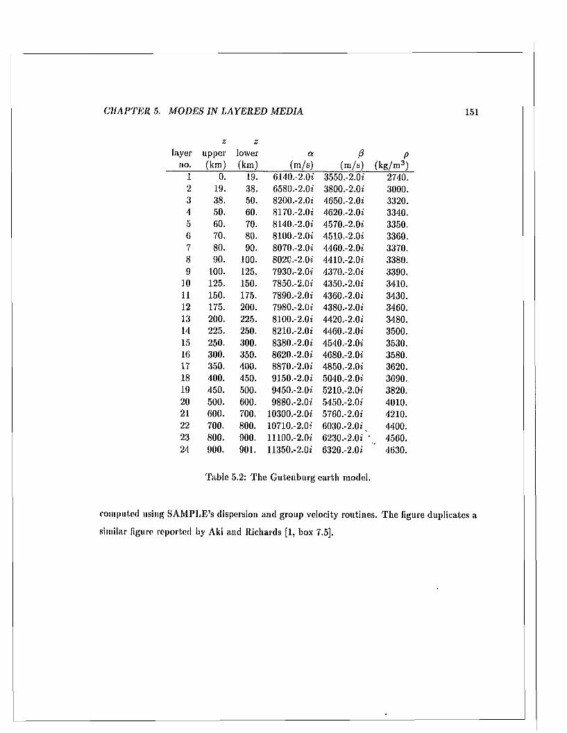
C H A P TE R 5. M O D ES IN L A Y E R E D M ED IA 151
z 2tyer upper lower a P Pno. (km) (km) (m /s) (m /s) (k g /m 3)
1 0. 19. 6140.-2.0i 3550.-2.0i 2740.2 19. 38. 6580.-2.0i 3800.-2.0i 3000.3 38. 50. 8200.-2.0i 4650.-2.0i 3320.4 50. 60. 8170.-2.0i 4620.-2.0i 3340.5 60. 70. 8140.-2.0i 4570.-2.0i 3350.6 70. 80. 8100.-2.0i 4510.-2.0i 3360.7 80. 90. 8070.-2.0i 4460.-2.0i 3370.8 90. 100. 802C.-2.0i 4410.-2.0i 3380.9 100. 125. 7930,-2.0i 4370.-2.0i 3390.
10 125. 150. 7850.-2.0i 4350.-2.0i 3410.11 150. 175. 7890.-2.0i 4360.-2.0i 3430.12 175. 200. 7980.-2.0i 4380.-2.0i 3460.13 200. 225. 8100.-2.0i 4420.-2.0i 3480.14 225. 250. 8210.-2.0i 4460.-2.0i 3500.15 250. 300. 8380.-2.0i 4540.-2.0i 3530.16 300. 350. 8620.-2.0i 4680.-2.0i 3580.17 350. 400. 8870.-2.0i 4850.-2.0i 3620.18 400. 450. 9150.-2.0i 5040.-2.0i 3690.19 450. 500. 9450.-2.0i 5210.-2.0i 3820.20 500. 600. 9880.-2.0i 5450.-2.0i 4010.21 600. 700. 10300.-2.0i 5760.-2.0i 4210.22 700. 800, 10710.-2.Oi 6030.-2.0i, 4400.23 800. 900. 11100.-2.0i 6230.-2.0i ’ 4560.24 900. 901. 11350.-2.Oi 6320.-2.0i 4630.
Table 5.2: The G utenburg earth model.
computed using SA M PLE’S dispersion and group velocity routines. T he figure duplicates a
similar figure reported by Aid and Richards [1, box 7.5].

152
SAMPLE: Layer Profile Gutenburg Earth Model
200
£ 400
Q.
600
800
4000 6000 8000 10000 12000
P- and S-wave Speed (m/s) Density (kg/m**3)
Figure 5.11: Wave speed and density profile in the Gutenburg earth model: P-wave speed is the solid line, S-wave speed the dashed, and density the dotted.
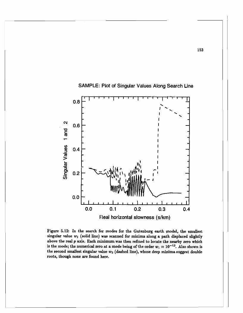
153
SAMPLE: Plot of Singular Values Along Search Line
CM
"Oc<a
coCD
CO>k -_co3O)cCO
0.8
0.6
0.4
0.2
0.0
0.0 0.1 0.2 0.3 0.4Heal horizontal slowness (s/km)
Figure 5.12: In the search for modes for the Gutenburg earth model, the smallest singular value wy (solid line) was scanned for minima along a path displaced slightly above the real p axis. Each minimum was then refined to locate the nearby zero which is the mode; the numerical zero at a mode being of the order w\ « 10-t3 . Also shown is the second smallest singular value W2 (dashed line), whose deep minima suggest double roots, though none are found here.

154
SAMPLE: Complex Slowness Plane
0.03000
0.02500
^ 0.02000 (/>
w w Q) cICO5? 0.01000E
0.01500
0.00500
0 .0 0 0 0 00.050 0.100 0.150 0.200 0.250 0.300
Real Slowness (s/km)
Figure 5.13: P-SV mode locations for the Gutenburg earth model at 0.05 Hz. Proper modes are indicated by circular dots, and improper by square. The solid lines are the P and S branch lines. Proper modes to the left of the S-wave branch point (pr = 0.1582 s/km) are well behaved S-leaky modes.
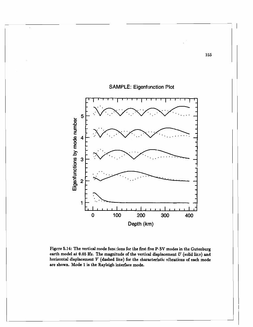
155
SAMPLE: Eigenfunction Plot
a>£ 2
E3Ca>SE£w co*5o c3C05o>
LU
5
4
3
2
1
0 100 200 300 400Depth (km)
Figure 5.14: The vertical mode functions for the first five P-SV modes in the Gutenburg earth model at 0.05 Hz. The magnitude of the vertical displacement U (solid line) and horizontal displacement V (dashed line) for the characteristic vibrations of each mode are shown. Mode 1 is the Rayleigh interface mode.
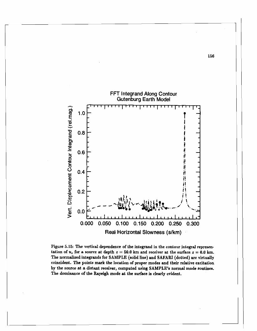
156
FFT Integrand Along Contour Gutenburg Earth Model
d>(0E<D
T3C(0
0.8O)<Dc
0.63O+*coO*- 0.4§ECDP ^ « w 0.2 o.wsi o.o >
0.000 0.050 0.100 0.150 0.200 0.250 0.300Real Horizontal Slowness (s/km)
Figure 5.15: The vertical dependence of the integrand in the contour integral representation of uz for a source at depth z = 50.0 km and receiver at the surface z = 0.0 km. The normalized integrands for SAMPLE (solid line) and SAFAHI (dotted) are virtually coincident. The points mark the location of proper modes and their relative excitation by the source at a distant receiver, computed using SAMPLE’S normal mode routines. The dominance of the Rayeigh mode at the surface is clearly evident.
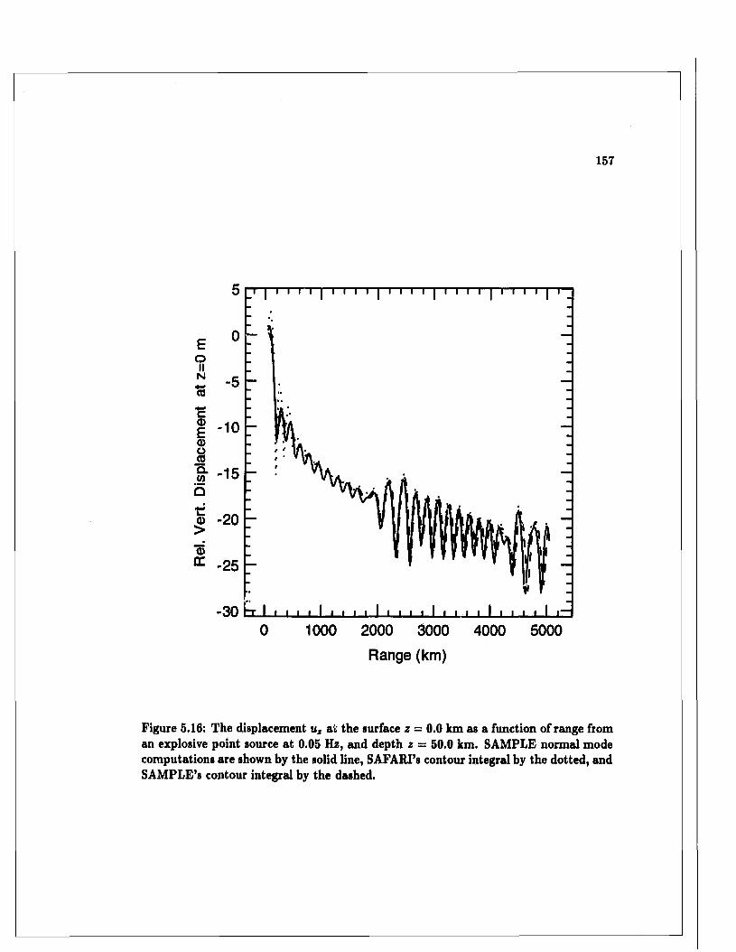
EoiiN«54-rf
I -10a>
jo
& * 15Q
©* -25
-300 1000 2000 3000 4000 5000
Range (km)
Figure 5.16: The displacement uz at the surface z = 0.0 km as a function of range from an explosive point source at 0.05 Hz, and depth z ~ 50.0 km. SAMPLE normal mode computations are shown by the solid line, SAFABl’s contour integral by the dotted, and SAMPLE’S contour integral by the dashed.
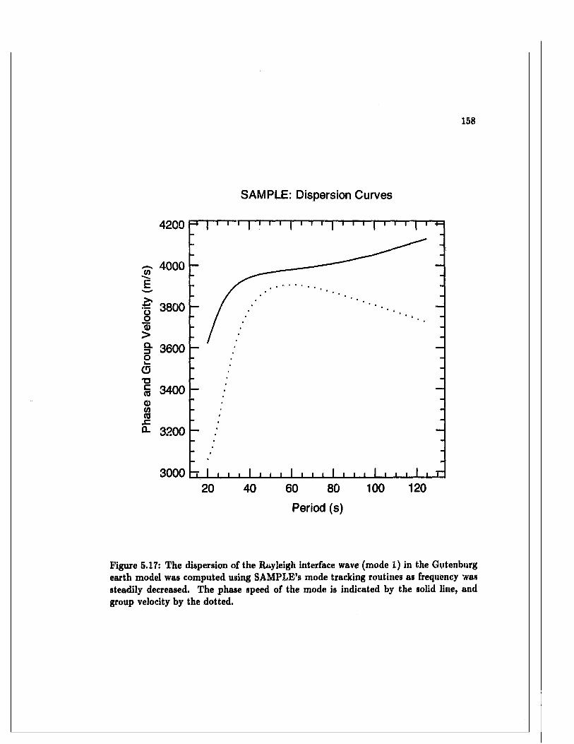
158
4200
SAMPLE: Dispersion Curves
-4" | r i i | 7 i i | ' i i i | i r.i j ' i 7 i r"4—
~ 4000
E, r
• | 3800
15>§■ 36000 >_CD
1 3400 ®
3200
! |3000 “T 1 I I i 1 l i i 1 i i i 1 i i i 1 I I I 1 I T
20 40 60 80 100 120
Period (s)
Figure 5.17: The dispersion of the Rayleigh interface wave (mode 1) in the Gutenburg earth model was computed using SAMPLE’S mode tracking routines as frequency was steadily decreased. The phase speed of the mode is indicated by the solid line, and group velocity by the dotted.
159
C h a p t e r 6
Catalogue o f normal m odes
If our goal is to understand the physics of wave propagation using modes, or if we
hope to exploit the advantages of modes in numerical models, the analysis m ust be brought
to a practical level where, by inspection, we are able to quickly estim ate 1) w hat modes are
likely to exist, 2) which of those will be im portant for a given application, and 3) where
the modes are likely to be in the complex slowness plane. To be conversant this way, we
m ust (list nam e and classify modes according to their im portan t properties, relating them
to the properties of the waveguide using general rules of thum b. I have tried to condense
this vast topic into a single chapter, to give an indication of the wide variety of modes tha t
can exist in layered media, to predict where they are to be found in the complex plane, and
to present properties about modes th a t I have not found in the literature . The examples I
include have been chosen to dem onstrate lesser-known properties of norm al modes.
Textbook treatm ents of modes in oceanic waveguides usually develop their subject
starting with the elem entary oceanic waveguide consisting of a single homogeneous fluid
layer, and build up to the two layer (Pekeris) model, thereby dem onstrating m any aspects
of normal modes in their simplest context. The approach provides an excellent introduction,
but the jum p to many layered waveguides having solid m edia with absorption is a big one,
requiring a more general approach th a t treats modes simply as reverberant cylindrical waves,
and th a t is how I proceed here.
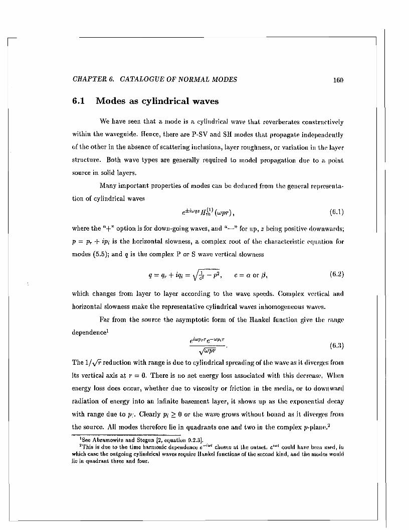
C H A P TE R 6. C A TA LO G U E OF N O R M A L M OD ES 160
6.1 M odes as cylindrical w aves
We have seen th a t a mode is a cylindrical wave th a t reverberates constructively
within the waveguide. Hence, there are P-SV and SH modes th a t propagate independently
of the o ther in the absence of scattering inclusions, layer roughness, or va.ria.tion in the layer
structure. Both wave types are generally required to model propagation due to a point
source in solid layers.
Many im portan t properties of modes can be deduced from the general representa
tion of cylindrical waves
e±iwqzn £ ) ( u p r ) > (6.1)
where the “+ ” option is for down-going waves, and ” for up, 2 being positive downwards;
p = pr + ipi is the horizontal slowness, a complex root of the characteristic equation for
modes (5.5); and q is the complex P or S wave vertical slowness
q = qr + % = - p2, c = a or /J, (6.2)
which changes from layer to layer according to the wave speeds. Complex vertical and
horizontal slowness make the representative cylindrical waves inhomogeneous waves.
Far from the source the asym ptotic form of the Hankel function give the. range
dependence1picuprT e -u ip ir
The 1 /y / r reduction with range is due to cylindrical spreading of the wave as it diverges from
its vertical axis a t r = 0. There is no net energy loss associated with this decrease, When
energy loss does occur, whether due to viscosity or friction in the media, or to downward
radiation of energy into an infinite basement layer, it shows up as the exponential decay
with range due to p\. Clearly />; > 0 or the wave grows without bound as it diverges from
the source. All modes therefore lie in quadrants one and two in the complex p-plane.2
'See Abrainowitz and Stegun [2, equation 9.2,3],2This is due to the tim e harm onic dependence c~ 'wt chosen a t the outset, c,uH could have been used, in
which case the outgoing cylindrical waves require Hankel functions of the second kind, and the modes would lie in quadran t three and four,
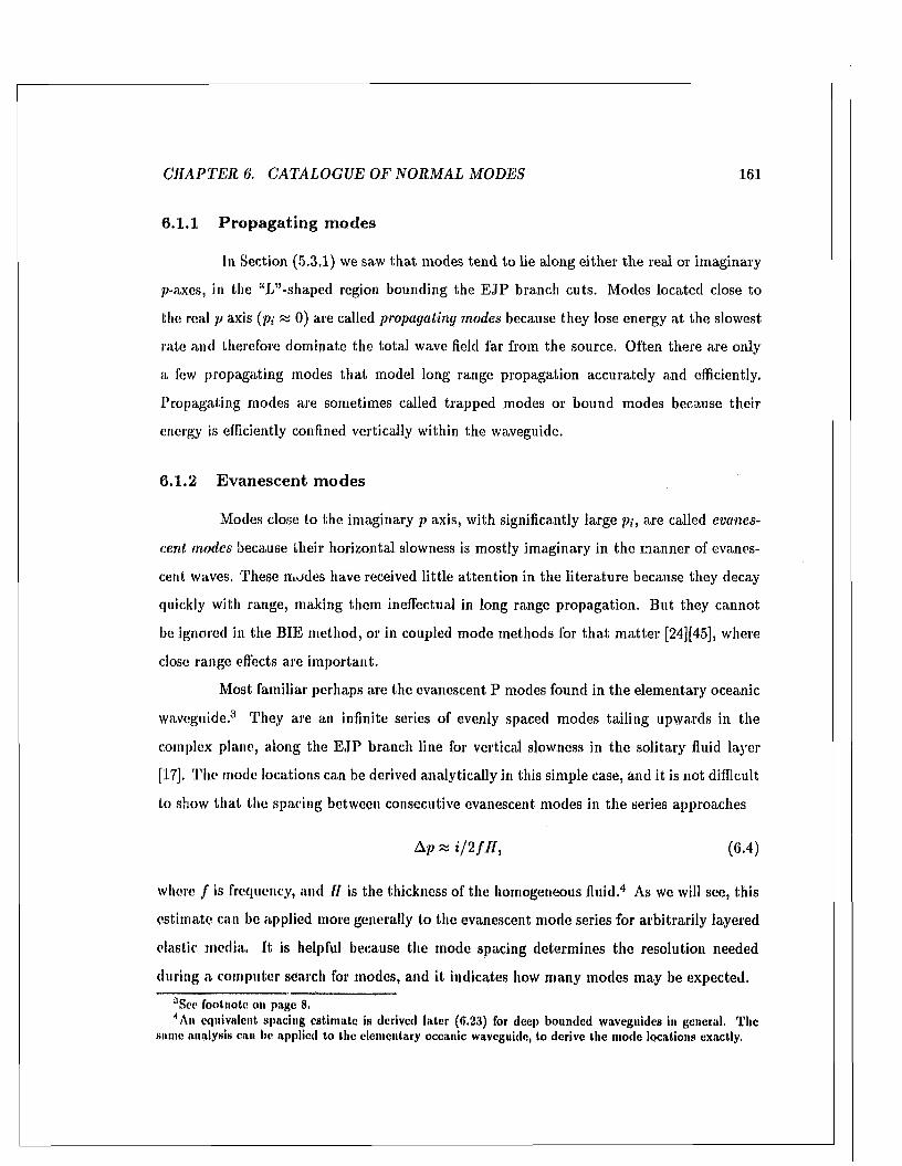
C H A P T E R 6. C ATA LO G U E OF N O R M A L MO D ES 161
6.1.1 Propagating m odes
In Section (5.3.1) we saw th a t modes tend to lie along either the real or im aginary
p-axes, in the “L”-shaped region bounding the E JP branch cuts. Modes located close to
the real p axis {pi fa 0) are called propagating modes because they lose energy at the slowest
rate and therefore dom inate the to tal wave field far from the source. Often there are only
a few propagating modes th a t model long range propagation accurately and efficiently.
Propagating modes are sometimes called trapped modes or bound modes because their
energy is efficiently confined vertically within the waveguide.
6.1.2 Evanescent modes
Modes close to the im aginary p axis, with significantly large pi, are called evanes
cent modes because their horizontal slowness is mostly im aginary in the m anner of evanes
cent waves. These modes have received little atten tion in the lite ra tu re because they decay
quickly with range, making them ineffectual in long range propagation. But they cannot
be ignored in the B IE m ethod, or in coupled mode m ethods for th a t m atte r [24][45], where
close range effects are im portant.
Most familiar perhaps are the evanescent P modes found in the elementary oceanic
waveguide.3 They are an infinite series of evenly spaced modes tailing upwards in the
complex plane, along the E JP branch line for vertical slowness in the solitary fluid layer
[17]. T he inode locations can be derived analytically in this simple case, and it is not difficult
to show th a t the spacing between consecutive evanescent modes in the series approaches
Ap « i / 2 fH , (6.4)
whore / is frequency, and I f is the thickness of the homogeneous fluid .'1 As we will see, this
estim ate can be applied more generally to the evanescent mode series for arbitrarily layered
elastic media. I t is helpful because the mode spacing determ ines the resolution needed
during a com puter search for modes, and it indicates how m any modes m ay be expected.
aSee footnote on page 8,4An equivalent spacing estim ate is derived later (6.23) for deep bounded waveguides in general. The
same analysis can be applied to the elementary oceanic waveguide, to derive the mode locations exactly,

C H A P T E R 6. C A TA LO G U E OF NORMAL MODES 162
Less familiar perliaps, are the evanescent P-SV modes found in a homogeneous
solid p late with free boundaries. These modes occur in two infinite series on both sides of
the im aginary slowness axis [90] [6] [51] as shown in Fig. (6.1) for a 3 m ice plate. In a
lossless homogeneous plate, these evanescent modes occur in symmetric pairs each mode in
the first quadrant having a sym m etric counterpart in the second quadrant ,but absorption
or additional layers disturbs this symmetry. A t greater frequencies the evanescent P-SV
modes lie closer to the im aginary axis. The m ode locations cannot be derived analytically
in this case, b u t the spacing estim ate (6.4) for evanescent modes still applies. In the 3 m
ice plate at 750 Hz or example, A p « i j (2 X 750 X 3) = 0.222? s/km , which compares well
with the actual spacing in the two sym m etric inode series in Fig. (6.1). Evanescent; plate
modes occur very often in geoacoustics, for it would appear th a t all plate-like structures
bands of undivided solid layers spanning a finite thickness, but not touching a solid half
space— behave like plates to some degree.
To illustrate , Fig.(6.2) shows p art of the evanescent mode series for the Arctic
profile of Table (5.1) considered earlier. The higher order evanescent inodes (larger p;)
separate into three distinct series: 1) water-borne modes along the imaginary axis, 2) closely
spaced bottom -borne modes on both sides of the imaginary axis th a t appear to swirl around
the axis, and 3) widely spaced ice-borne modes on both sides of the imaginary axis, only
two of which are shown in the figure. This thick bottom layer and the thin ice layer plain
structures giving rise to evanescent m odes on both sides of the imaginary axis, T he swirling
pattern of the bottom -borne m ode locations is due to interactions between the bottom and
water column. T he swirls get larger and less pronounced as jn increases, eventually settling
into two unswerving lines on both sides of the imaginary axis. The depths at which the
modes are active—w hether in the w ater (200 in thick), bottom (2000 m), or ice (3m) were
determ ined by plotting the vertical m ode functions, and confirmed using the estim ated
mode spacing (6.4) for evanescent modes a t 20 Ifz:
A p ~ i j (2 x 20 x 200) = 0.125? s/km lor the w ater column,
A p « i j (2 x 20 X 2000) = 0.0125? s/km for the deep bottom plate, (6.5)
A p « i j (2 x 20 x 3) = 8.333? s/krn for the thin ice plate,
These agree with vertical spacings found for the three evanescent mode series in Fig.(0.2),
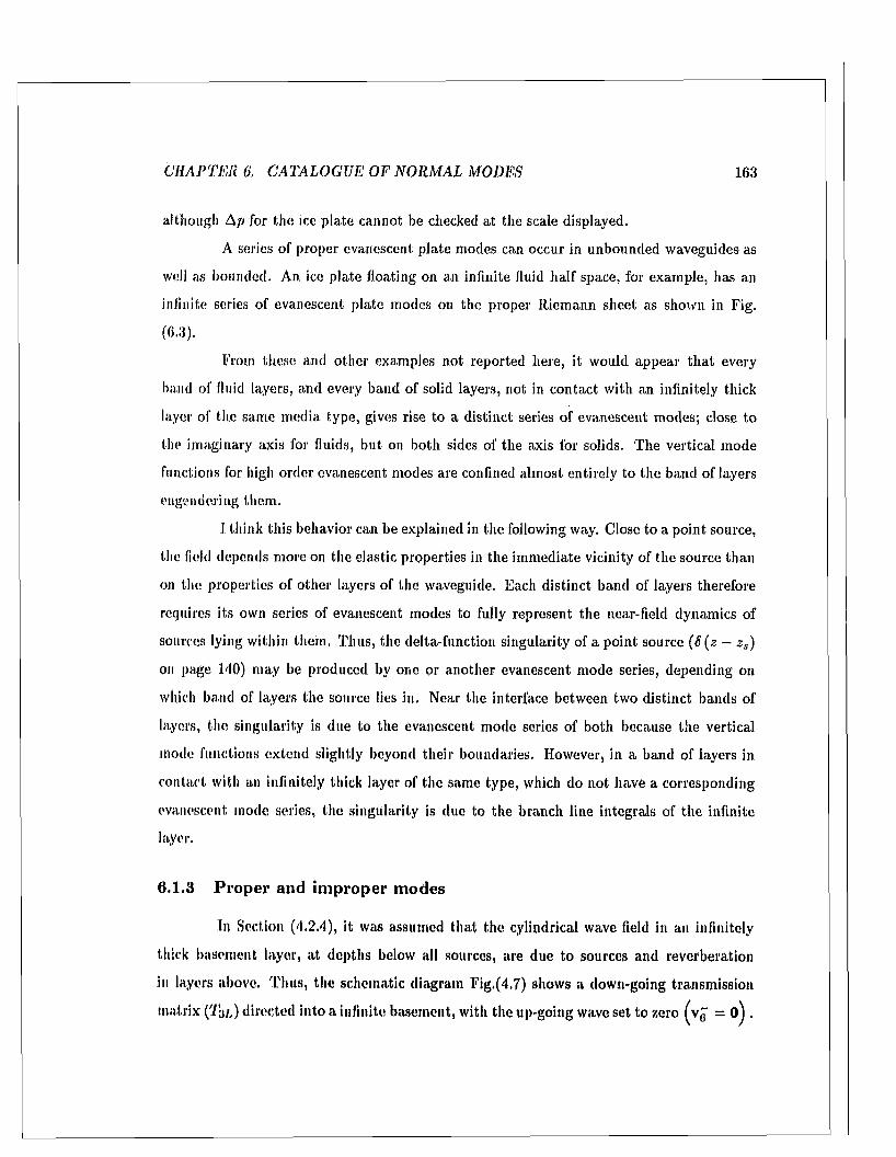
C H A P TE R 6. C A TA LO G U E OF N O R M A L MODES 163
although Ap for the ice p late cannot be checked at the scale displayed.
A series of proper evanescent p late modes can occur in unbounded waveguides as
well as bounded. An ice p late floating on an infinite fluid half space, for example, has an
infinite series of evanescent plate modes on the proper Riem ann sheet as shown in Fig.
(6.3).
From these and other examples not reported here, it would appear th a t every
band of fluid layers, and every band of solid layers, not in contact with an infinitely thick
layer of the same m edia type, gives rise to a distinct series of evanescent modes; close to
the im aginary axis for fluids, but on both sides of the axis for solids. The vertical mode
functions for high order evanescent modes are confined almost entirely to the band of layers
engendering them.
I think this behavior can be explained in the following way. Close to a point source,
the field depends m ore on the elastic properties in the im m ediate vicinity of the source than
on the properties of other layers of the waveguide. Each distinct band of layers therefore
requires its own series of evanescent modes to fully represent the near-field dynamics of
sources lying within them. Thus, the delta-function singularity of a point source (S (z - za)
on page 140) may be produced by one or another evanescent mode series, depending on
which band of layers the source lies in. Near the interface between two distinct bands of
layers, the singularity is due to the evanescent mode series of both because the vertical
mode functions extend slightly beyond their boundaries. However, in a band of layers in
contact with an infinitely thick layer of the same type, which do not have a corresponding
evanescent mode series, the singularity is due to the branch line integrals of the infinite
layer.
6.1.3 Proper and improper m odes
In Section (4.2.4), it was assumed th a t the cylindrical wave field in an infinitely
thick basement layer, a t depths below all sources, are due to sources and reverberation
in layers above. T hus, the schematic diagram Fig.(4.7) shows a down-going transm ission
matrix (Taj,) directed into a infinite basement, with the up-going wave set to zero ( v j = 0].

164
Ejx.13
(/>coCDc£o
COO)coE
m —i i—m
Real Slowness (s/km)
CDjQE3zCD
~oo2
s -COco'■5c3
L L(D
■oO
COO‘■ECD>
8
7
6
5
4
3
2
1
0.0 0.5 1.0 1.5 2.0 2.5 3.0Depth (m)
Figure 6.1: Top: The P-SV (circular dots) and SH (square dots) modes for a free ice plate: a = 3300 - 30.0* m /s, /? = 1730 - 20.0i m /s, p = 900 kg/m :\ thickness i f ~ 3.0 m, and / = 750.0 Hz. Bottom: The vertical mode functions for the first 7 P-SV modes marked by crosses above, ordered by decreasing real slowness. Shown are the real (solid line) and imaginary (dotted line) parts of the vertical displacement U for each mode.
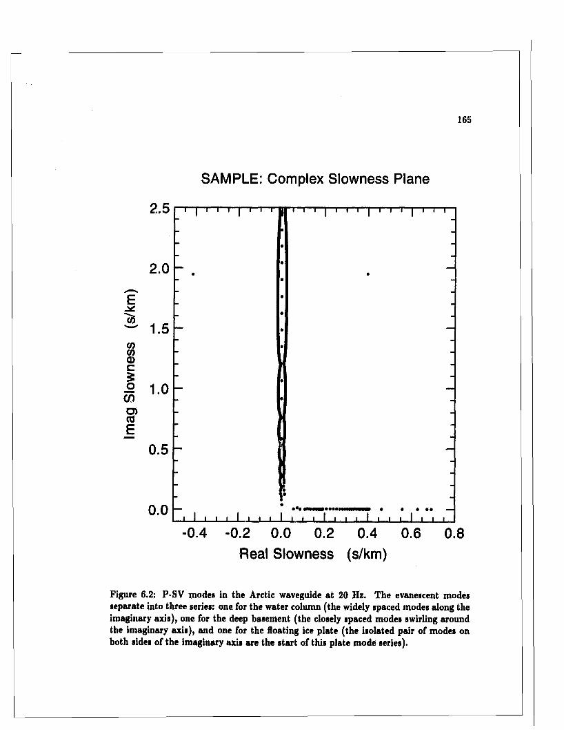
165
SAMPLE: Complex Slowness Plane
2.5
2.0
E05
030)0c5OCO03COE
0.5
0.0 • • •
0.4 -0.2 0.0 0.2 0.4 0.6 0.8Real Slowness (s/km)
Figure 6.2: P-SV modes in the Arctic waveguide at 20 Hz. The evanescent modes separate into three series: one for the water column (the widely spaced modes along the imaginary axis), one for the deep basement (the closely spaced modes swirling around the imaginary axis), and one for the floating ice plate (the isolated pair of modes on both sides of the imaginary axis are the start of this plate mode series).
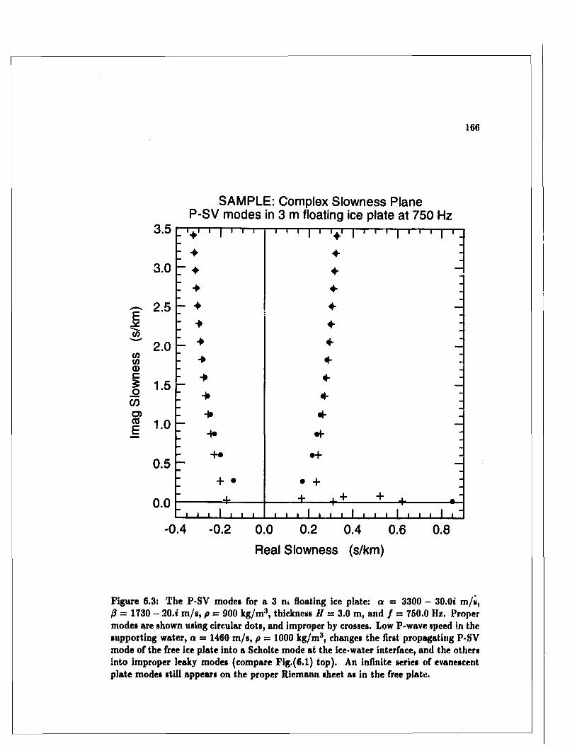
166
E
ww0>c5o
COo>coE
3.5
3.0
2.5
2.0
1.5
SAM PLE: Complex Slowness Plane P -S V modes in 3 m floating ice plate at 750 Hz
0.5
0.0
7T71 1..[" 1 1 1 i i i | i i j |.t r-r—[—r r i | i
♦
--
,— “F- _
4--
4- —
-
H* 4-— —: -»• * :-
+• •+— —- -
: + • • + :+ + _|_ + + _j_ f
I i i i i- i l l 1 i * i 1 j,.l—L 1 1 1 1 1..1.L. I I I I 1-0.4 -0 .2 0 .0 0.2 0.4 0.6 0.8
Real Slowness (s/km)
Figure 6.3: The P-SV modes for s 3 m floating ice plate: a = 3300 ~ 30.01 m /s, /? = 1730 - 20.* m /s, p — 900 kg/m 3, thickness H = 3.0 m, and / t= 750.0 Hz. Proper modes are shown using circular dots, and improper by crosses. Low P-wave speed in the supporting water, a = 1460 m /s, p = 1000 kg/m3, changes the first propagating P-SV mode of the free ice plate into a Scholte mode at the ice-water interface, and the others into improper leaky modes (compare Fig.(6.1) top). An infinite series of evanescent plate modes still appears on the proper Riemann sheet as in the free plate.
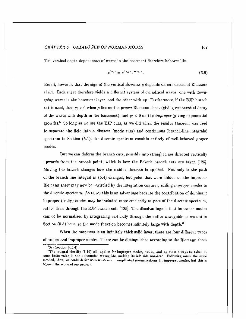
C H A P T E R 6. C A TA LO G U E OF N O R M A L MOD ES 167
The vertical depth dependence of waves in the basement therefore behaves like
e iuqz _ e iwqTz e -w qiZ' (g g )
Recall, however, th a t the sign of the vertical slowness q depends on our choice of Riemann
sheet. Each sheet therefore yields a different system of cylindrical waves: one w ith down-
going waves in the basement layer, and the other with up. Furtherm ore, if the E JP branch
cut is u.Jed, then </; > 0 when p lies on the proper Riemann sheet (giving exponential decay
of the waves with depth in the basem ent), and m < 0 on the improper (giving exponential
grow th).5 So long as we use the E JP cuts, as we did when the residue theorem was used
to separate the field into a discrete (m ode sum) and continuous (branch-line integrals)
spectrum in Section (5.1), the discrete spectrum consists entirely of well-behaved proper
modes.
But we can deform the branch cuts, possibly into straight lines directed vertically
upwards from the branch point, which is how the Pekeris branch cuts are taken [125].
Moving the branch changes how the residue theorem is applied. Not only is the path
of the branch line integral in (5.4) changed, but poles th a t were hidden on the im proper
Riemann sheet may now be ■ncircled by the integration contour, adding improper modes to
the discrete spectrum . A t ti, this is an advantage because the contribution of dom inant
im proper (leaky) modes m ay be included more efficiently as p a rt of the discrete spectrum ,
ra ther than through the E JP branch cuts [125], The disadvantage is th a t im proper modes
cannot Ire normalized by integrating vertically through the entire waveguide as we did in
Section (5.5) because the mode function becomes infinitely large with d ep th .6
W hen the basement is an infinitely thick solid layer, there are four different types
of proper and im proper modes. These can be distinguished according to the Riemann sheet
6Sre Section (4.2,4),"The integral identity 15.10) still applies for im proper modes, but z,\ and zn m ust always be taken at
some finite value in tlie unbounded waveguide, making its left side non-zero. Following much the same method, then, we could derive som ewhat more complicated norm alizations for im proper modes, bu t this is beyond the scope of my project.
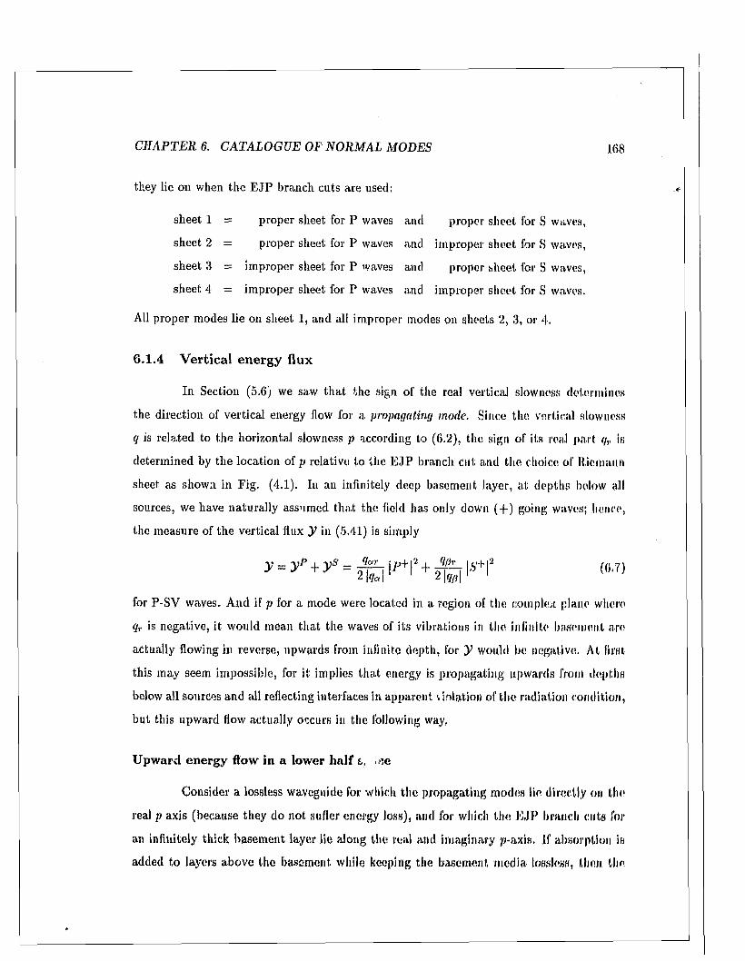
C H A P T E R 6. C A TA LO G U E OF N O R M A L MODES 168
they lie on when the E JP branch cuts are used:
sheet 1 = proper sheet for P waves and proper sheet for S waves,
sheet 2 = proper sheet for P waves and im proper sheet for S waves,
sheet 3 = im proper sheet for P waves and proper sheet for S waves,
sheet 4 = im proper sheet for P waves and im proper sheet for S waves.
All proper modes lie on sheet 1, and all im proper modes on sheets 2, 3, or 4.
6.1.4 Vertical energy flux
In Section (5.6) we saw th a t the sign of the real vertical slowness determines
the direction of vertical energy flow for a propagating mode. Since the vertical slowness
q is related to the horizontal slowness p according to (6.2), the sign of its real part qr is
determ ined by the location of p relative to the E JP branch cut and the choice of Riemann
sheet as shown in Fig. (4.1). In an infinitely deep basement layer, a t depths below all
sources, we have naturally assumed th a t the field has only down (+ ) going waves; hence,
the m easure of the vertical flux y in (5.41) is simply
y y p + y s = |p+12 + JUjl. 15+12 (a 7)y ^ 2 \qa \ ' I 2 \qp\ ' '
for P-SV waves. A nd if p for a mode were located in a region of the complex plane where
qT is negative, it would mean tha t the waves of its vibrations in the infinite basement are
actually flowing in reverse, upwards from infinite depth, for y would be negative. At first
this m ay seem impossible, for it implies th a t energy is propagating upwards from depths
below all sources and all reflecting interfaces in apparent violation of the radiation condition,
but this upward flow actually occurs in the following way.
Upward energy flow in a lower half £,, ce
Consider a lossless waveguide for which the propagating modes lie directly on the
real p axis (because they do not suffer energy loss), and for which the E JP branch cuts for
an infinitely thick basem ent layer lie along the real and imaginary p-axis. If absorption is
added to layers above the basement while keeping the basement m edia lossless, then the
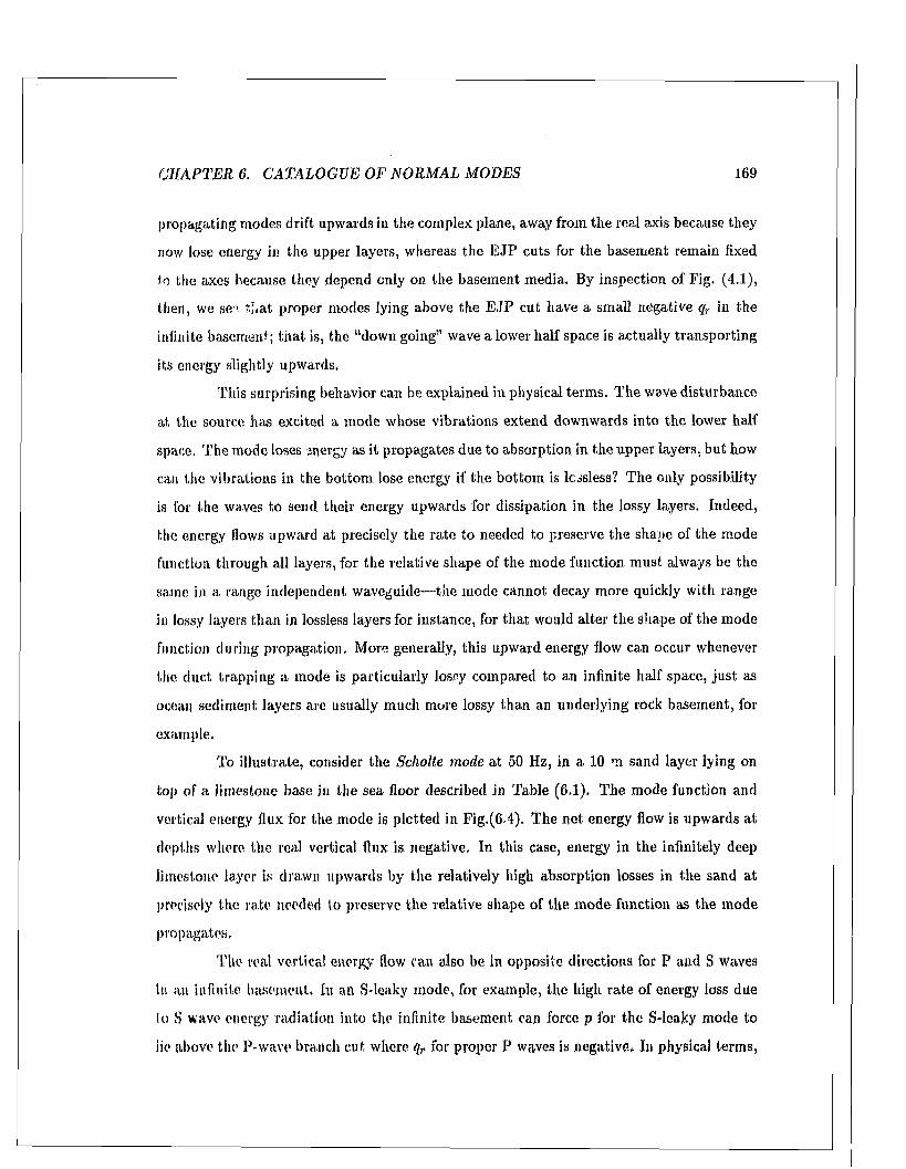
C H A P T E R 6. C ATA LO G U E OF N O R M A L M O D ES 169
propagating modes drift upwards in the complex plane, away from the real axis because they
now lose energy in the upper layers, whereas the E JP cuts for the basement remain fixed
to the axes because they depend only on the basement media. By inspection of Fig. (4.1),
then, we see ?.,\at proper modes lying above the E JP cut have a small negative qr in the
infinite basement; th a t is, the “down going” wave a lower half space is actually transporting
its energy slightly upwards.
This surprising behavior can be explained in physical term s. T he wave disturbance
a t the source has excited a m ode whose vibrations extend downwards into the lower half
space. T he mode loses energy as it propagates due to absorption in the upper layers, but how
can the vibrations in the bottom lose energy if the bottom is lossless? The only possibility
is for the waves to send, their energy upwards for dissipation in the lossy layers. Indeed,
the energy flows upward at precisely the ra te to needed to preserve the shape of the mode
function through all layers, for the relative shape of the m ode function m ust always be the
same in a range independent waveguide—the m ode cannot decay more quickly with range
in lossy layers than in lossless layers for instance, for th a t would alter the shape of the mode
function during propagation. More generally, this upward energy flow can occur whenever
the duct trapping a mode is particularly losry compared to an infinite half space, ju s t as
ocean sediment layers are usually m uch more lossy than an underlying rock basement, for
example.
To illustrate, consider the Scholte mode a t 50 Hz, in a 10 m sand layer lying on
top of a limestone base in the sea floor described in Table (6.1). T he mode function and
vertical energy flux for the m ode is plotted in Fig.(6.4). T he net energy flow is upwards at
depths where the real vertical flux is negative. In this case, energy in the infinitely deep
limestone layer is drawn upwards by the relatively high absorption losses in the sand at
precisely the ra te needed to preserve the relative shape of the m ode function as the mode
propagates,
T he veal vertical energy flow can also be in opposite directions for P and S waves
in an infinite basement. In an S-leaky mode, for example, the high ra te of energy loss due
lo 8 wave energy radiation into the infinite basem ent can force p for the S-leaky mode to
lie above the P-wave branch cut where qT for proper P waves is negative. In physical term s,
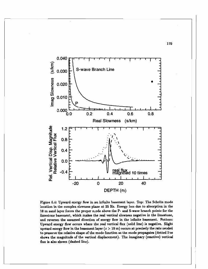
170
0.040
« 0.030v>V)S 0.020
o, 0.010
©T53
0 .0 0 0
1.2
wave Branch
0.2 0.4 0.6Real Slowness (s/km)
Q .~.12 fc Q >
0.4
0.0
© ®>CE -0.4"®DC
(8 © O >
—- | “t— i— 1“ r
: ............ • ■ • ' ' A .
t— t— |— i— i— r— p— i— r —
, ' \ j
L 1
1 1__ J__________ 1___1----magnted 1 0 times ~
i i 1 i i i 1 i «— "
-20 0 20 DEPTH (m)
40
Figure 8.4: Upward energy flow in an infinite basement layer. Top: The Scholte mode location in the complex slowness plane at 25 Hz. Energy Iocs due to absorption in the 10 m sand layer forces the proper mode above the P- and S-wave branch points for the limestone basement, which makes the real vertical slowness negative in the limestone, and reverses the assumed direction of energy flow in the infinite basement. Bottom: Upward energy flow occurs where the real vertical flux (solid line) is negative. Slight upward energy flow in the basement layer (z > 10 m) occurs at precisely the rate needed to preserve the relative shape of the mode function as the mode propagates (dotted line shows the magnitude of the vertical displacement). The imaginary (reactive) vertical flux is also shown (dashed line).
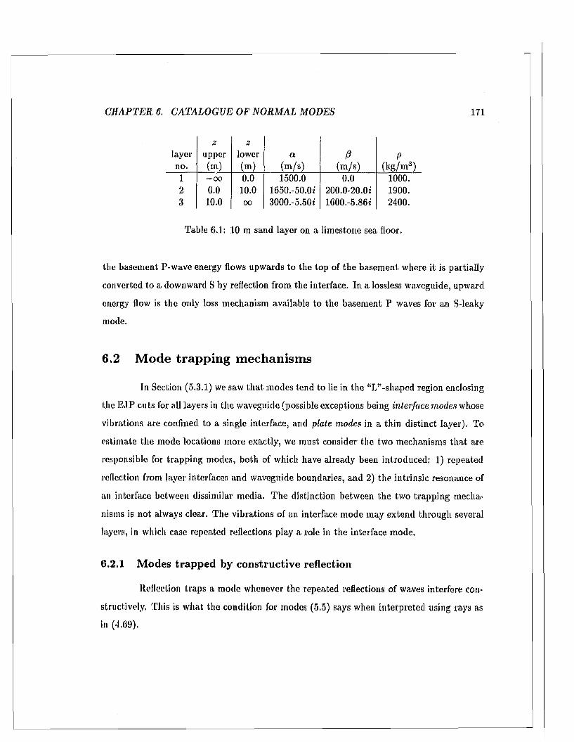
C H A P T E R 6. C A TA LO G U E OF N O R M A L M OD ES 171
z zlayer upper lower a P Pno. (m) (m) (m /s) (m /s) (kg /m 3)1 — 00 0.0 1500.0 0.0 1000.2 0.0 10.0 1650.-50.0i 200.0-20.0i 1900.3 10.0 OO 3000.-5.50i 1600.-5.86i 2400.
Table 6.1: 10 m sand layer on a limestone sea floor.
the basement P-wave energy flows upwards to the top of the basem ent where it is partially
converted to a downward S by reflection from the interface. In a lossless waveguide, upward
energy flow is the only loss mechanism available to the basem ent P waves for an S-leaky
mode.
6.2 M ode trapping m echanism s
In Section (5.3.1) we saw th a t modes tend to lie in the “L”-shaped region enclosing
the E JP cuts for all layers in the waveguide (possible exceptions being interface modes whose
vibrations are confined to a single interface, and plate modes in a th in distinct layer). To
estim ate the mode locations more exactly, we m ust consider the two mechanisms th a t are
responsible for trapping modes, both of which have already been introduced: 1) repeated
reflection from layer interfaces and waveguide boundaries, and 2) the intrinsic resonance of
an interface between dissimilar media. T he distinction between the two trapping mecha
nisms is not always clear. The vibrations of an interface mode m ay extend through several
layers, in which case repeated reflections play a role in the interface mode,
6.2.1 M odes trapped by constructive reflection
Reflection traps a m ode whenever the repeated reflections of waves interfere con
structively, This is w hat the condition for modes (5.5) says when in terpreted using rays as
in (4.69).
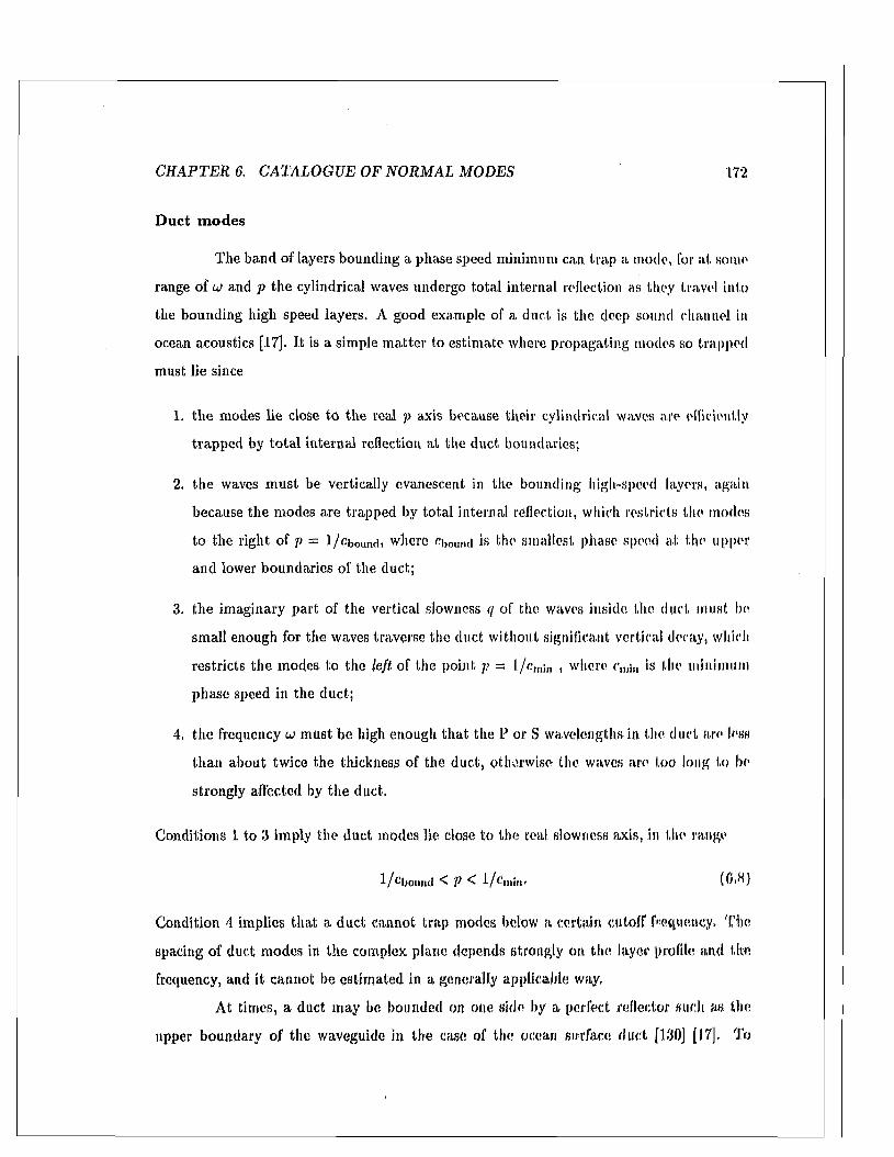
C H A P T E R 6. C A TA LO G U E OF N O R M A L M O D ES 172
D u c t m o d e s
The band of layers bounding a phase speed minimum can trap a mode, lor a t some
range of u) and p the cylindrical waves undergo to tal internal reflection as they travel into
the bounding high speed layers. A good example of a duct is the deep sound channel in
ocean acoustics [17]. It is a simple m atter to estim ate where propagating modes so trapped
must lie since
1. th e modes lie close to the real p axis because their cylindrical waves are efficiently
trapped by to ta l internal reflection a t the duct boundaries;
2. the waves m ust be vertically evanescent in the bounding high-speed layers, again
because the modes are trapped by to tal internal reflection, which restricts the inodes
to the right of p = l/cbound» where Cbound is the smallest phase speed a t the upper
and lower boundaries of the duct;
3. the im aginary p art of the vertical slowness q of the waves inside the duct must be
small enough for the waves traverse the duct without significant vertical decay, which
restricts the modes to the left of the point p = 1 /c m;M , where e,„jt, is the minimum
phase speed in the duct;
4. the frequency u m ust be high enough th a t the P or S wavelengths in the duct are less
than about twice the thickness of the duct, otherwise the waves are too long to be
strongly affected by the duct.
Conditions i to 3 imply the duct modes lie close to the real slowness axis, in tin* range
l / c Uoiind K p K I /c ntin- (0.H)
Condition 4 implies th a t a duct cannot trap modes below a certain cutoff frequency. The
spacing of duct modes in the complex plane depends strongly on the layer profile and the
frequency, and it cannot be estim ated in a generally applicable way.
A t times, a duct m ay be bounded on one side by a perfect reflector such as, the
upper boundary of the waveguide in the case of the ocean surface duct [130] [J7]. To
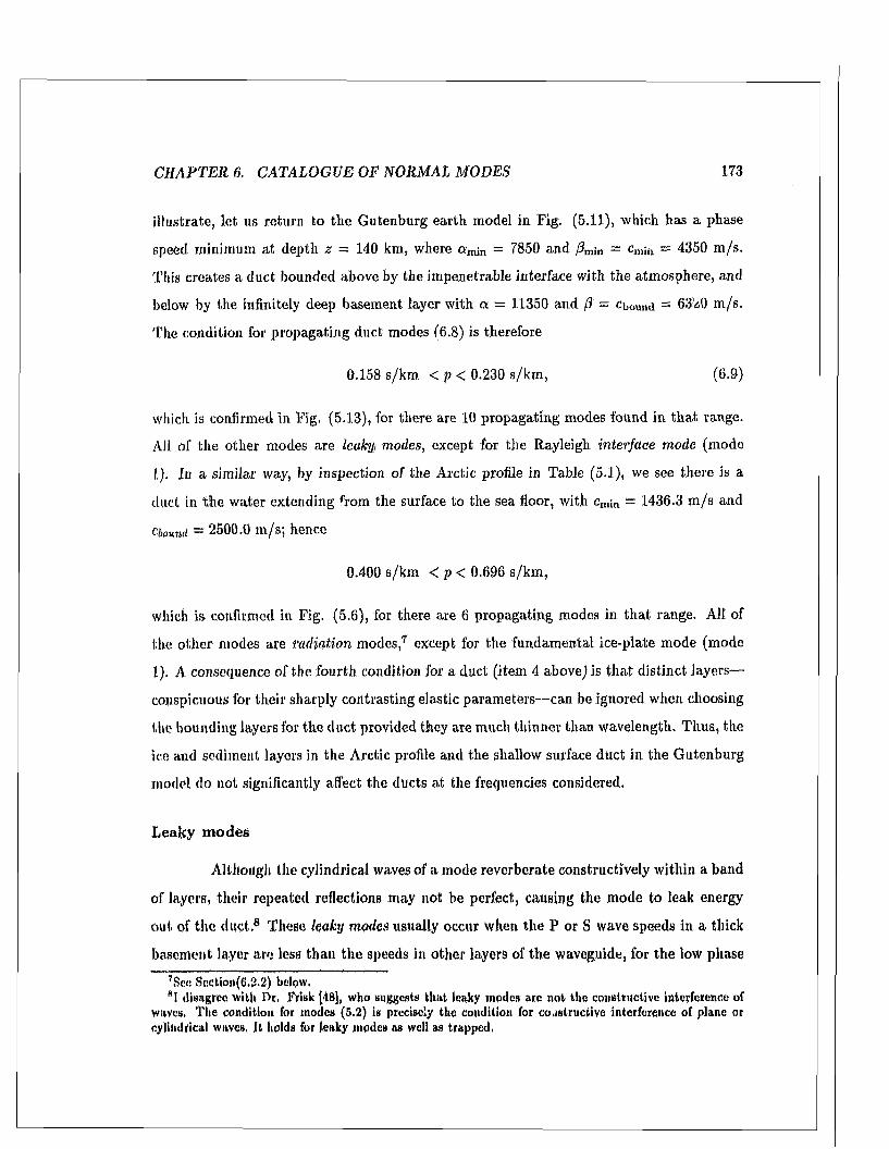
C H A P T E R 6. C A TA LO G U E OF N O R M A L M O D ES 173
illustrate, let us return to the G utenburg earth model in Fig. (5.11), which has a phase
speed minimum at depth z = 140 km, where a m;n = 7850 and /3m jn = cmin = 4350 m /s.
This creates a duct bounded above by the im penetrable interface with the atm osphere, and
below by the infinitely deep basement layer with a — 11350 and (1 = Cbound = 6320 m /s.
The condition for propagating duct modes (6.8) is therefore
0.158 s/km < p < 0.230 s/km , (6.9)
which is confirmed in Fig. (5.13), for there are 10 propagating modes found in th a t range.
All of the o ther modes are leaky) modes, except for the Rayleigh interface mode (mode
1). In a similar way, by inspection of the Arctic profile in Table (5.1), we see there is a
duct in th e water extending from the surface to the sea floor, with c„un = 1436.3 m /s and
rb o u n d = 2500.0 m /s; hence
0.400 s/km < p < 0.696 s/km ,
which is confirmed in Fig. (5.6), for there are 6 propagating modes in th a t range. All of
the o ther modes are radiation m odes,7 except for the fundam ental ice-plate m ode (mode
1). A consequence of the fourth condition for a duct (item 4 above) is th a t distinct layers—
conspicuous for their sharply contrasting elastic param eters—can be ignored when choosing
the bounding layers for the duct provided they are m uch thinner than wavelength. T hus, the
ice and sediment layers in the Arctic profile and the shallow surface duct in the G utenburg
model do not significantly affect the ducts at the frequencies considered.
Leaky modes
Although the cylindrical waves of a mode reverberate constructively within a band
of layers, their repeated reflections may not be perfect, causing the m ode to leak energy
ou t of the du ct.8 These leaky modes usually occur when the P or S wave speeds in a thick
basement layer are less than the speeds in o ther layers of th e waveguide, for th e low phase
7Sce Section(6,2.2) below,®I disagree w ith I>r, Frisk [48], who suggests th a t leaky inodes are n o t the constructive interference of
waves. T he condition for modes (5.2) is precisely the condition for co.istructive interference of plane or cylindrical waves. I t holds for Jeaky modes as well as trapped.
C H A P T E R 6. C A TA LO G U E OF N O R M A L M O D ES 174
speeds prevents to ta l in ternal reflection a t the top interface of th e basement. Leaky inodes
are usually much weaker th an propagating modes far from the source due to their energy
loss, b u t they can dom inate the field far from the source in the absence of propagating
modes [42]. Estim ating where leaky modes should lie is more difficult than trapped modes
because the lower bound in (6.8) does no t apply in the absence of to ta l internal reflection.
They are also relatively far from the real slowness axis due to their high energy loss.
There are three types of leaky modes nam ed according to the leaking wave type:9
if the basem ent layer is solid, there are S-leaky modes, and PS-leaky modes; if the basement
layer is a fluid, there are only P-leaky modes. P-leaky modes do not occur with solid
basements for S waves invariably leak when P waves do since a > /3. In lossless media, all
leaky modes lie on im proper Riemann sheets—S-leaky modes on Riemann sheet 2, PS-leaky
on sheet 4, and P-leaky on sheet 3—causing their mode functions to grow exponentially with
depth. For when the basem ent is lossless, its E JP cuts lie along the real and im aginary axes
of the complex p-plane, and the dual requirem ent tha t the mode lose energy (p; > 0)and
th a t the radiated energy travel downwards in the basement (qr > 0) , imply th a t p lie on
an im proper R iem ann sheet as shown by Fig. 4.'1). Im proper leaky modes only occur
in unbounded waveguides because the im penetrable boundaries of the bounded waveguide
ultim ately trap the energy radiated out of the duct. But in a deep bounded waveguide there
are radiation modes th a t correspond very closely to the leaky modes in the unbounded case
as we m ight expect.10
Proper leaky modes
I t was surprising to find tha t leaky modes can be transferred to the proper Riemann
sheet by absorption in the infinite basem ent layer, Recall th a t energy absorption is added
to a half space by adding a small negative imaginary part to the P and S phase speeds,11
which shifts the E JP branch cuts away from the real p axis. If the absorption is great
enough, i t is possible for the branch cu t to pass over some leaky modes, transferring them
from the im proper sheet to the proper sheet. In effect, the exponential growth due to
°The suggestion to nam e leaky modes this way is due to Zhang [137].J0See Section (6,2.2).(1See Section(2,2).
C H A P T E R 6. C ATA LO G U E OF N O R M A L MOD ES 175
leakage in a lossless half space is overcome by exponential decay due to energy absorption.
The relatively high absorption typical of low-speed shear waves in ocean sediment layers is
often sufficient to place the dom inant S-leaky modes on the proper Riem ann sheet. All of
the S-leaky modes reported by Tindle and (N .R .)Chapm an [126] are proper modes for this
reason ,12 as are the modes reported by Ellis and (M .F.)Chapm an [42]. Though instances
of proper leaky modes can be found in the literature, they have appeared w ithout specific
m ention, presumably because leaky modes are always assum ed to be im proper modes, as
they arc in the lossless waveguide commonly used in introductory treatm ents.
Proper leaky modes are of interest for modeling purposes, for norm al m ode pro
grams designed for proper modes with complex p, which ordinarily cannot handle leaky
modes due to their poorly behaved mode functions, should be able to handle proper leaky
modes w ithout modification. In fact, it m ay be justified to add artificially high absorption
in the basement to make a leaky mode environm ent amenable to a proper mode program .
We have already encountered proper leaky modes in the G utenburg earth model
in Fig. (5.13), where the artificial absorption added to the basem ent layer displaced the
S-wave branch line far enough to pass over some S-leaky modes, transferring them from the
improper Riemann sheet to the proper. For a more realistic example for ocean acoustics,
consider the two layer leaky-mode environment used by Ellis and Chapm an [42], detailed
in Table (6.2). T he mode locations a t 200 IIz are shown in Fig. (6.5). In this case the
realistic S-wave absorption of the chalk sea floor is enough to transfer all of the leaky modes
to a proper Riemann sheet for S-waves (Riemann sheet 1 or 3). The exponential decay with
depth of a proper leaky mode is evident in Fig. (6.6), In the absence of absorption in the
basement they would grow exponentially with depth.
laTi»<llc and C hapm an call the five modes left of the P-wave branch point in their Fig.(2) “trapped inodes” since, lying close to the real axis, the modes suffer little energy loss, B ut the modes are S-Icaky nonetheless, for they are Imperfectly trapped by the low shear wave speed in the bottom half space; 0 = C50 m /s with absorption 0,2 dD/A in the basement, compared with a = 1500 m /s in the w ater column. T he leakage is very weak because the large a : 0 contrast prevents the leaking shear waves in th e bottom from being strongly excited, In the absence of absorption in the bottom , these modes would be im proper inodes because the E JP branch cut for S-wavcs would slip down over these modes, transfering them to the im proper Riemann sheet 2,
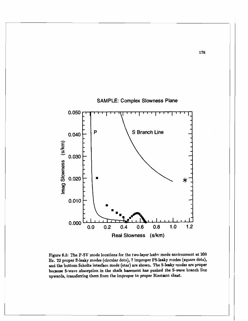
176
SAMPLE: Complex Slowness Plane
0.050 i i rr n r | i r iy~y f i i - p r i -i | i r i ] i i i [~
E
0.040
0.030V)
(Dc
% 0.020 S' E
0.010
0 .0 0 0
S Branch Line
0.0 0.2 0.4 0.6 0.8 1.0 1.2
Real Slowness (s/km)
Figure 6.5: The P-SV mode locations for the two-layer leakv mode environment at 200 Hz. 22 proper S-leaky modes (circular dots), 7 improper PS-leaky mode* (square dots), and the bottom Scholte interface mode (star) are shown. The S-leaky modes are proper because S-wave absorption in the chalk basement has pushed the S-wave branch line upwards, transferring them from the improper to proper Riemann sheet.
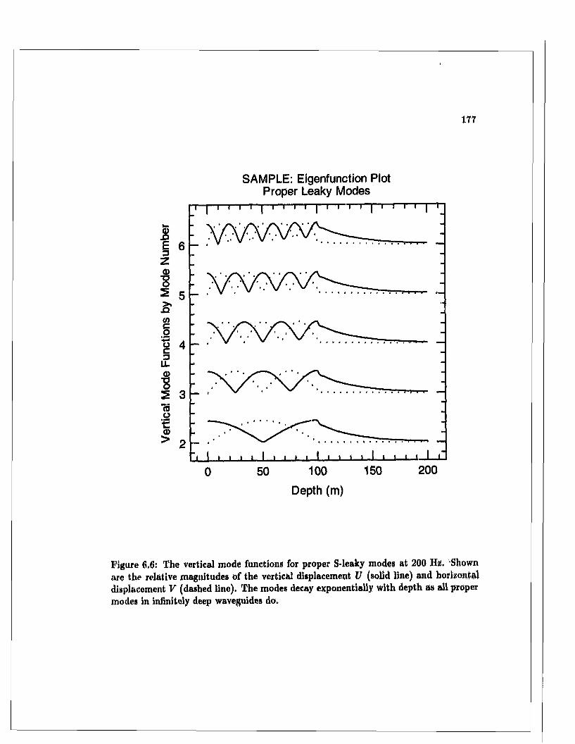
177
SAMPLE: Eigenfunction Plot Proper Leaky Modes
2E3zd)85
jaCOc o
■ ■ §c3
LLd>■8srto
■■£d>>
6
5
4
3
2
150 200100500
Depth (m)
Figure 6.6: The vertical mode functions for proper S-leaky modes at 200 Hz. Shown are the relative magnitudes of the vertical displacement U (solid line) and horizontal displacement V (dashed line). The modes decay exponentially with depth as all proper modes in infinitely deep waveguides do.
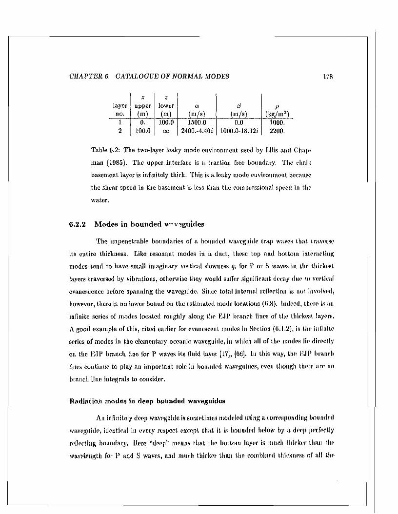
C H A P T E R 6. C A TA LO G U E OF N O R M A L MODES 178
layerz
upper**
lower a 13 f>110. (m) (m) (m /s) (m /s) (kg/m 3)1 0. 100.0 1500.0 0.0 1000. “2 100.0 oo 2400.-4,40/ 1000.0-18.32/ 2200.
Table 6.2: Tlie two-layer leaky mode environment used by I'lllis and Chap
m an (1985). The upper interlace is a traction free boundary. T he chalk
basem ent layer is infinitely thick. This is a leaky mode environm ent because
the shear speed in the basement is less than the cornpressional speed in the
water.
6.2.2 M odes in bounded w *v’guides
The im penetrable boundaries of a bounded waveguide trap waves tha t traverse
its en tire thickness. Like resonant modes in a duct, these top and bottom interacting
modes tend to have small im aginary vertical slowness <n for P or S waves in the thickest
layers traversed by vibrations, otherwise they would suffer significant decay due to vertical
evanescence before spanning the waveguide. Since total internal reflection is not involved,
however, there is no lower bound on the estim ated mode locations (0.8). Indeed, there is an
infinite series of modes located roughly along the E JP branch lines of the thickest layers,
A good example of this, cited earlier for evanescent modes in Section (6.1.2), is the infinite
series of modes in the elem entary oceanic waveguide, in which all of the inodes lie directly
on the E JP branch line for P waves its fluid layer [17], [66], In this way, the EJP branch
lines continue to play an im portan t role in bounded waveguides, even though there are no
branch line integrals to consider.
Radiation modes in deep bounded waveguides
An infinitely deep waveguide is sometimes modeled using a corresponding hounded
waveguide, identical in every respect except that it is bounded below by a deep perfectly
reflecting boundary. Here “deep'1' means that the bottom layer is much thicker than the
wavelength for H and S waves, and much thicker than the combined thickness of all the
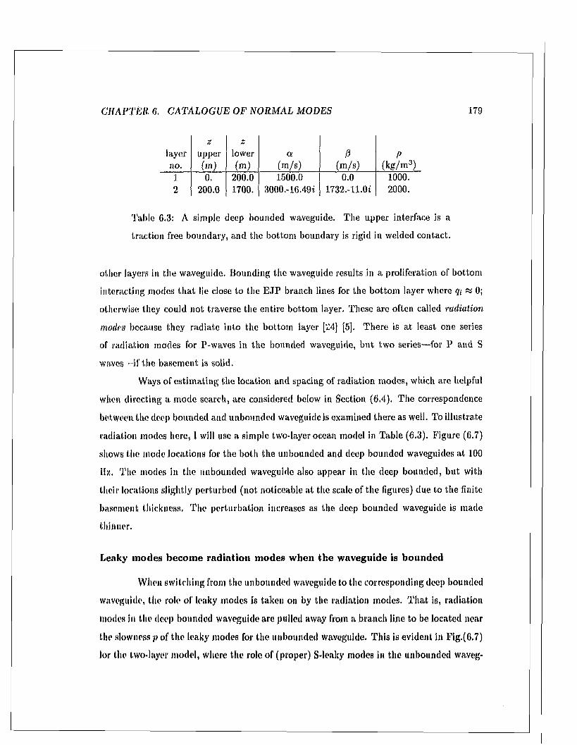
C H A P T E R 6. C A TA LO G U E OF N O R M A L M OD ES 179
z zlayer upper lower a /3 Pno. (m ) (m) (m /s) (m /s) (k g /m 3)
1 0. 200.0 1500.0 0.0 1000.2 200.0 1700. 3000.-16.49i 1732.-ll.0 i 2000.
Table 6.3: A simple deep bounded waveguide. The upper interface is a
traction free boundary, and the bottom boundary is rigid in welded contact.
other layers in the waveguide. Bounding the waveguide results in a proliferation of bottom
interacting modes th a t lie close to the E JP branch lines for the bottom layer where </; « 0;
otherwise they could no t traverse the entire bottom layer. These are often called radiation
modes because they rad ia te into the bottom layer [24] [5]. T here is a t least one series
of radiation modes for P-waves in the bounded waveguide, bu t two series—for P and S
waves if the basem ent is solid.
Ways of estim ating the location and spacing of radiation modes, which are helpful
when directing a mode search, are considered below in Section (6.4). T he correspondence
between the deep bounded and unbounded waveguide is examined there as well. To illustrate
radiation modes here, I will use a simple two-layer ocean model in Table (6,3). Figure (6,7)
shows the mode locations for the both the unbounded and deep bounded waveguides a t 100
I h . The modes in the unbounded waveguide also appear in the deep bounded, but with
their locations slightly perturbed (not noticeable a t the scale of the figures) due to the finite
basement thickness, The perturbation increases as the deep bounded waveguide is made
thinner.
Leaky inodes becom e radiation m odes w hen the w aveguide is bounded
When switching from the unbounded waveguide to the corresponding deep bounded
waveguide, the role of leaky modes is taken on by the radiation modes. That is, radiation
modes in the deep bounded waveguide are pulled away from a branch line to be located near
the slowness p of the leaky modes for the unbounded waveguide. This is evident in Fig.(6.7)
lor the two-layer model, where the role of (proper) S-leaky modes in the unbounded waveg-
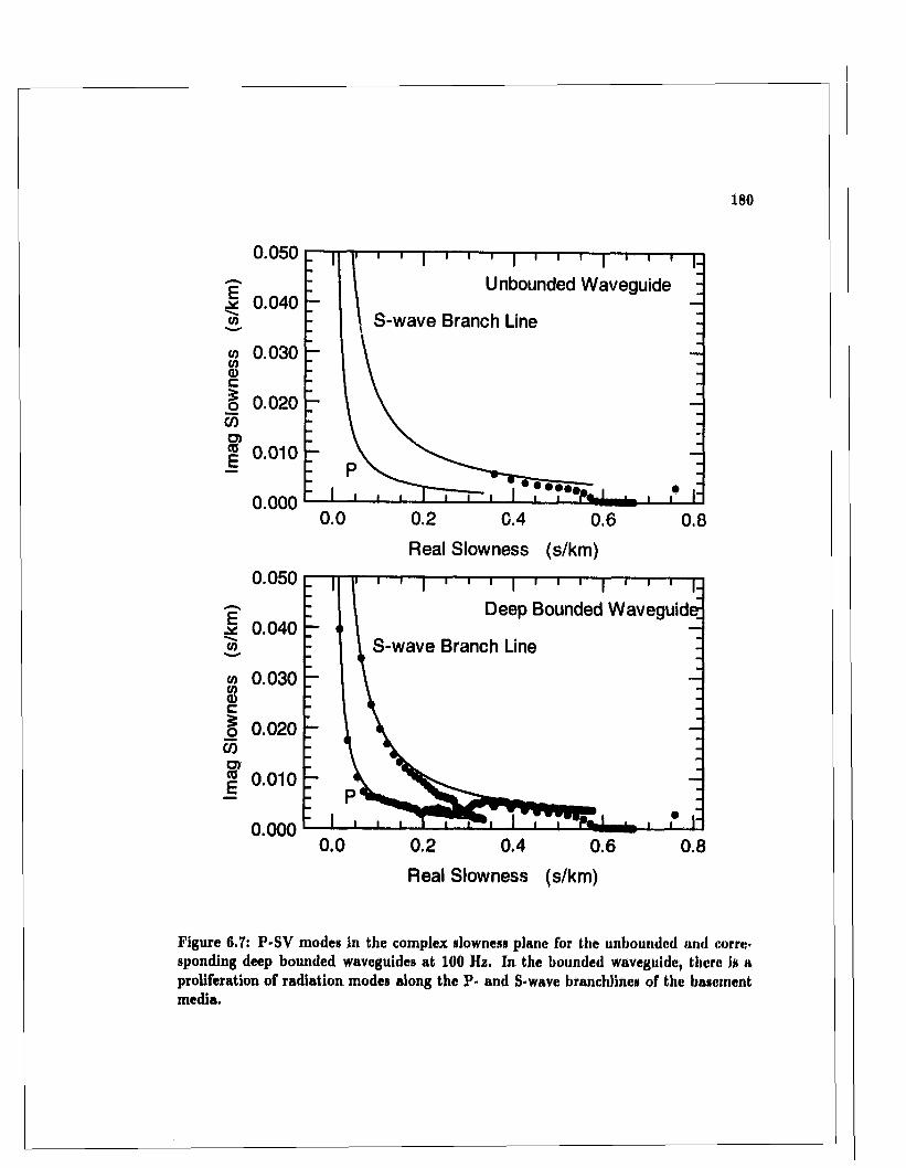
180
EXL—, W
CO(0d>c1CO
S'E
0.050
Unbounded Waveguide0.040
S-wave Branch Line
0.030
0.020
0.010
0 .0 0 00.0 0.2 0.4 0.6 0.8
COCOd)c1C/3
S'E
Real Slowness (s/km)
0.050
Deep Bounded Waveguide;0.040
S-wave Branch Line
0.030
0.020
0.010
0 .0 0 00.0 0.2 0.4 0.6
Real Slowness (s/km)
0.8
Figure 6.7; P-SV modes in the complex slowness plane for the unbounded and corresponding deep bounded waveguides at 100 Hz. In the bounded waveguide, there is a proliferation of radiation modes along the P- and S-wave branchlines of the basement media.
C H A P T E R 6. C A TA LO G U E OF NORMA.L MODES 181
uide is taken on by radiation modes in the deep bounded waveguide. Fig.((i.S) shows th a t
the vertical mode function for one proper leaky mode and its corresponding radiation mode
are virtually identical. A similar correspondence occurs between dom inant improper leaky
modes lying above the S-wave branch line, and radiation modes pulled upwards away from
the line to fill the role of the leaky mode. This correspondence suggests th a t im proper leaky
modes in an unbounded waveguide, whose mode function grow exponentially with depth,
could be replaced by closely m atched radiation modes of the corresponding deep bounded
waveguide, whose m ode function is well behaved with depth.
6 .2 .3 I n t e r f a c e m o d e s
An interface mode is the resonance of an interface due to a discontinuity in the
layered media, ra th e r than the repeated constructive reflection of waves between interfaces.
Like gravity waves a t the surface of w ater, they entail elliptical particle motion in a vertical
plane parallel to the direction of travel[66, sect. 8.4.3] [127], This precludes interface modes
consisting of strictly P waves in fluid m edia since their motion is irrotational, and of SH
waves in solid since their m otion is horizontal, leaving only the possibility of P-SV interface
modes. T he characteristic vibrations of an interface m ode are maximal at the reverberating
interface.
Rayleigh mode
An interface mode due to a traction free boundary on a solid is called a Rayleigh
mode, T he free boundary of a homogeneous solid half space always supports one, and only
one, propagating Rayleigh mode. I t is nondispcrsive, and its horizontal slowness of the
mode typically lies in the range13
1 .0 5 ^ < p < 1.2 i (0.10)
The situation is m ore complicated when the mode interacts with o ther layers in the waveg
uide because the wave is then dispersive. An oceanic waveguide having an infinitely deep
solid bottom , for example, supports a Rayleigh m ode a t very low frequencies (below 1 Hz)
laThe phase speed is typically 0.85 to 0.95 times the minimum phase speed c,n\„ in cither medium [127].
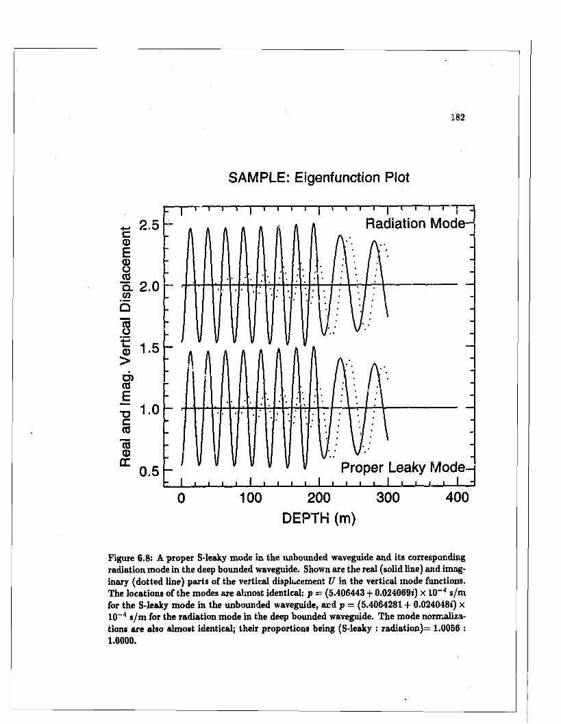
182
SAMPLE: Eigenfunction Plot
Radiation Mode2.oc0ECDO0o. 2 .0 (0b76o
0>d )(0E
• ocCO
750
CC Proper Leaky M ode-
4003002001 0 0
DEPTH (m)
Figure 6.8: A proper S-leaky mode in the unbounded waveguide and its corresponding radiation mode in the deep bounded waveguide. Shown are the real (solid line) and imaginary (dotted line) parts of the vertical displacement U in the vertical mode functions. The locations of the modes are almost identical: p = (5.406443 + 0.024069i) X 10- '1 s/m for the S-leaky mode in the unbounded waveguide, and p = (5.4064281 + 0.024048t) X 10- '1 s/m for the radiation mode in the deep bounded waveguide. The mode normalizations are also almost identical; their proportions being (S-leaky : radiation)= 1.0056 : 1.0000.
C H A P T E R 6. C A TA LO G U E OF N O R M A L M OD ES 183
when th e water column is th in compared with the wavelength, in which case /} in (6.10)
must be taken from deep w ithin the solid bottom . At higher frequencies, however, the
same Rayleigh m ode is likely to become a Scliolte mode (considered below) confined to the
ocean floor. We have already encountered a Rayleigh mode in the G utenburg earth model
in Section (5.8).
Scholte modes
An interface mode due to the discontinuity at a fluid-solid interface is called a
Scholte mode. T he interface between a fluid and solid half space always supports ju st one
propagating Scholte mode. I t is nondispersive, and its horizontal slowness must be
P > - ^ —{-------4 r (6.H )min (Osolid, Psolid, j
or else it radiates (leaks) energy. Thus, each fluid-solid interface in a waveguide supports a
Scholte mode when the wavelength is considerably less than the thickness of the adjacent
layers. A t longer wavelengths, however, the Scholte mode in teracts with o ther parts of the
waveguide, and is likely to become a different mode altogether, possibly a duct or radiation
mode. W e have already encountered a dispersive Scholte mode spanning a lossy sand layer
on the sea floor in Fig.(6.4).
Stonely modes
An interface mode due to the discontinuity at a solid-solid interface is called a
Stonely mode. Unlike Rayleigh and Scholte modes, Stonely modes rarely occur; they only
exist for narrow ranges of elastic param eters a , [3, and p for both m edia [6]. They have not
been found in seismology [127], nor have I encountered one in the course of this research.
Rayleigh mode o f the second kind
An interface mode due to a rigid boundary in welded contact with a solid also
exists, though it is always a leaky mode. This mode appears in gcoacoustics in an indirect
way, when the waveguide is bounded below by a rigid im penetrable reflector. Since the
waveguide is bounded, this leaky interface mode appears as a radiation mode at roughly
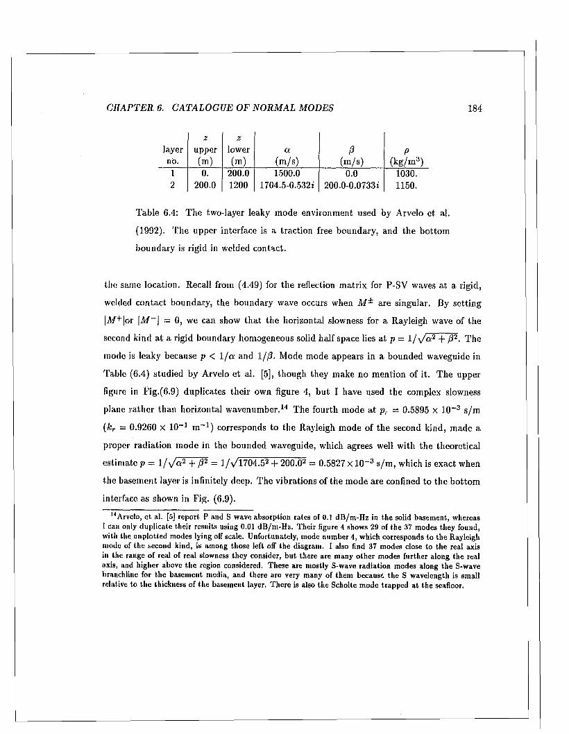
C H A P T E R 6. C A TA LO G U E OF N O R M A L M O D ES 184
z zlayer upper lower a 0 Pno. (m) (m) (m /s) (m /s) (kg /m 3)1 0. 200.0 1500.0 0.0 1030.2 200.0 1200 1704.5-0.532t 200.0-0.0733t 1150.
Table 6.4: T he two-layer leaky m ode environment used by Arvelo et al.
(1992). T he upper interface is a traction free boundary, and the bottom
boundary is rigid in welded contact.
the same location. Recall from (4.49) for the reflection m atrix for P-SV waves at a rigid,
welded contact boundary, the boundary wave occurs when are singular. By setting
|M + |or \ M ~ \ — 0, we can show th a t the horizontal slowness for a Rayleigh wave of the
second kind a t a rigid boundary homogeneous solid half space lies a t p = 1 /y /a t2 + 0 2. The
mode is leaky because p < 1/ a and 1/ /3. Mode mode appears in a bounded waveguide in
Table (6.4) studied by Arvelo et al. [5], though they make no m ention of it. The upper
figure in Fig.(6.9) duplicates their own figure 4, bu t I have used the complex slowness
plane ra th e r than horizontal wavenum ber.14 The fourth m ode a t p, = 0.5895 x 10⁻³ s /m
(kr = 0.9260 X 10⁻¹ m -1 ) corresponds to the Rayleigh mode of the second kind, m ade a
proper radiation m ode in the bounded waveguide, which agrees well with the theoretical
estim ate p = 1 / s / o F + W = 1 / v /1704,52 + 200.02 = 0.5827 X 10~3 s / m, which is exact when
the basement layer is infinitely deep. T he vibrations of the m ode are confined to the bottom
interface as shown in Fig. (6.9).
H Arvelo, e t al. [5] report P and S wave absorption rates of 0.1 dB /m -H z in the solid basem ent, whereasI can only duplicate their results using 0.01 dB /m -H z. Their figure 4 shows 29 of the 37 modes they found, with the unplotted modes lying off scale. Unfortunately, mode num ber 4, which corresponds to th e Rayleigh mode of the second kind, is among those left off the diagram. I also find 37 modes close to the real axis in the range of real of real slowness they consider, bu t there are many o ther modes further along the real axis, and higher above the region considered. These are mostly S-wave radiation modes along the S-wave branchlino for the basem ent media, and there are very many of them because the S wavelength is small relative to th e thickness of the basem ent layer. There is also the Scholte mode trapped a t the seafloor.
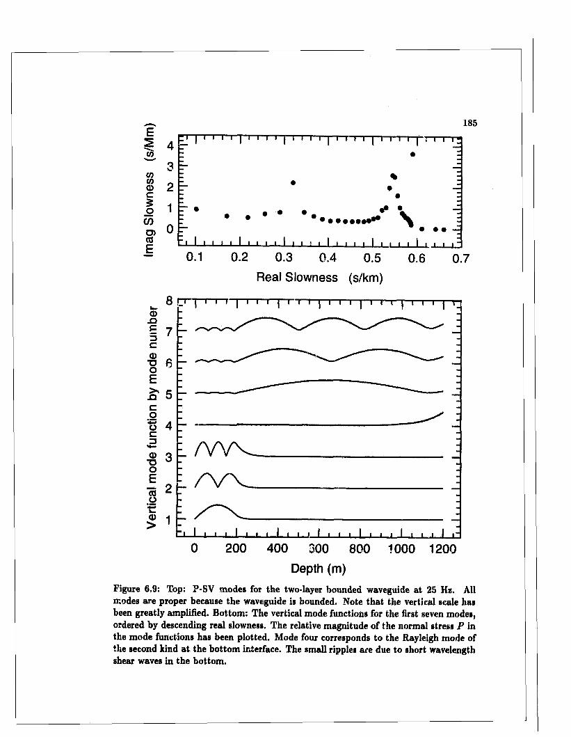
185
(0
WCOCDc$o
0303COE
4
3
21
• • • • • • \• • • •0
0.1 0.2 0.3 0.4 0.5 0.6 0.7
Real Slowness (s/km)
ox>p5ca)T3OE>»
JC3
oc13H—(UT3OECOorCD>
8
7
6
5
4
3
2
1
0 200 400 300 800 1000 1200
Depth (m)
Figure 6.9: Top: P-SV modes for the two-layer bounded waveguide at 25 Hz. All modes are proper because the waveguide is bounded. Note that the vertical scale has been greatly amplified. Bottom: The vertical mode functions for the first seven modes, ordered by descending real slowness. The relative magnitude of the normal stress P in the mode functions has been plotted. Mode four corresponds to the Rayleigh mode of the second kind at the bottom interface. The small ripples are due to short wavelength shear waves in the bottom.
C H A P T E R 6. C A TA LO G U E OF N O R M A L M O D ES 186
6.3 Identifying channels in th e channel m atrix m ethod
T he purpose of the channel m atrix m ethod is to accelerate the m ode search by
compressing the global m atrix before com puting its singular values, by combining com
ponents (layers and interfaces) in the schematic diagram together using the numerically
stable scattering m atrix m ethod. The only difficulty is to ensure th a t the compressed m a
trix remains sensitive to modes trapped at any depth in the waveguide. This requires th a t
the unknown wave vector for the compressed m atrix sample the field a t depths w ithin the
channel of every possible mode, where the vertical mode function for the m ode will be
significantly large. This can be done following two simple rules when combining elements.
Earlier in this chapter we saw th a t the boundary of an efficient duct occurs where
the cylindrical waves undergo to ta l internal reflection, which is where the waves switch
from being vertically propagating inside the duct (mostly real vertical slowness q), to being
vertically evanescent outside (mostly im aginary q). The first rule, then , is to re ta in the
unknown wave vectors a t every interface across which the P- or S-wave vertical slowness
change from being m ostly real in one layer to mostly im aginary in the o ther, for in this
way we ensure tha t the compressed m atrix will be sensitive to modes trapped in any duct,
A second rule is to re ta in the unknown wave vectors a t all interfaces th a t could possibly
support an interface m ode—im penetrable interfaces, and all interfaces between solid and
fluid layers—because th e vibrations of an interface m ode are certain to be significantly large
a t the interface trapping it,
We could, for example, s ta rt a t the top of the waveguide, and work downwards,
combining layers and their interfaces into a single scattering m atrix using the com bina
tion rules (4.65). W henever the complex nature of the vertical slowness in the next layer
changes—from dom inantly real to im aginary a t the boundary of a duct—the com bination
process is stopped and a new element is begun to retain the wave vector at the transm ission
depth as an unknown in the reduced ladder diagram for the waveguide. A new combined
element would also be started whenever the m edia changes from solid to fluid. T he com
bined elements are coupled using the continuity equation (4,42) for the interfaces between
them. To ensure interface modes are detected a t im penetrable boundaries, their boundary
C H A P T E R 6. C A TA LO G U E OF N O R M A L M O D ES 187
conditions for P-SV waves would be enforced using the basic forms: (4.46) for rigid bound
aries, and (4.48) for free, Since the vertical slowness depends on the horizontal slowness p,
the depths between components will change throughout a. mode search.
In this way, the Arctic profile in Table (5.1) is reduced to as few as five different
components—the free boundary, the ice plate, the w ater column, the solid sea floor, and
the deep rigid bottom , depending on the slowness p; ra ther than sixteen components in the
uncompressed waveguide: the free boundary, fourteen layers, and the deep rigid bottom.
The tim e savings due to compression are considerable. In this case, the time taken for a,
search for modes along the real slowness axis is almost exactly ten times longer using the
global m atrix than the channel m atrix m ethod.
6.4 D eep bounded w aveguides— T heory
A n unbounded oceanic waveguide is sometimes modeled by a corresponding bounded
waveguide identical in every respect except th a t it is bounded below by a deep perfectly re
flecting boundary. To approxim ate the unbounded case, the bounded basement layer must
be much thicker th an the wavelength for P and S waves in the basement media, and much
thicker than the combined thickness of all the o ther layers in the waveguide. The modes
characteristic of the deep bounded waveguide and its correspondence with the unbounded
waveguide are examined here.
6.4.1 R adiation m odes close to the EJP branch lines
Fig.(6,10) is a schematic diagram for the deep bounded waveguide when the wave
vectors are sampled a t the top and bottom of the basement layer. The upper reflection
m atrix R - is due to the layer structure above the basement layer (including the top interface
of the basem ent layer), and the lower reflection m atrix R + is due to the im penetrable
bottom . Up and down going wave vectors are transm itted equally through the homogeneous
basement layer by the transm ission m atrix (4.40)
T =g lU /r/u H Q
0(6 . 12)
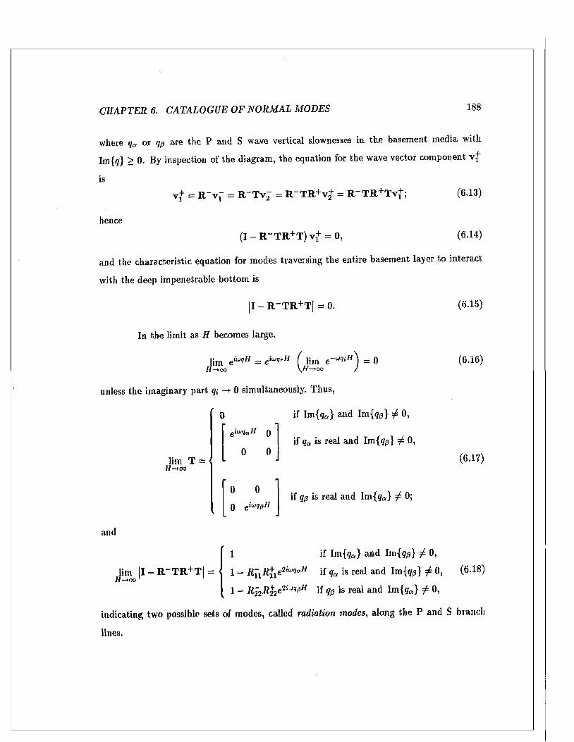
C H A P T E R 6. C ATA LO G U E OF N O R M A L MOD ES 188
where qa or qp are the P and S wave vertical slownesses in the basem ent m edia with
Im{r/} > 0. By inspection of the diagram , the equation for the wave vector com ponent v f
is
hence
v+ = R-v{- = R - T v j = R -T R + V + = R "T R + T v + ; (6.13)
(I - R" TR+ T) v f = 0, (6 • 14)
and the characteristic equation for modes traversing the entire basem ent layer to in teract
with the deep im penetrable bottom is
| I - R “TR+T| = 0. (6.15)
In the lim it as H becomes large.
lim eiwqH = eiu>qrH ( lim e- wqiIA = 0H—*oo \H—+oo /
unless the im aginary p art q, —> 0 simultaneously. Thus,
if Im{g&} and lm {qp} ^ 0,
if qa is real and I m - ^ } 7 0,
H - t 00
0eiuiqaH 0
0 0
0 0
0 eiwqPHif qp is real and Im {qa} 7 0;
and
lim jl-R " T R + T | = //— 1 '
(6.16)
(6.17)
1 if Im{ga } and lm {qp} ^ 0,
1 - R ^ R ^ e 2iuqafi if qa is real and lm {qp] 7 0, (6.18)
1 - R 2 2 R t 2 e2UqpH <l() is real and Im {9a) # °>
indicating two possible sets of modes, called radiation modes, along the P and S branch
lines.
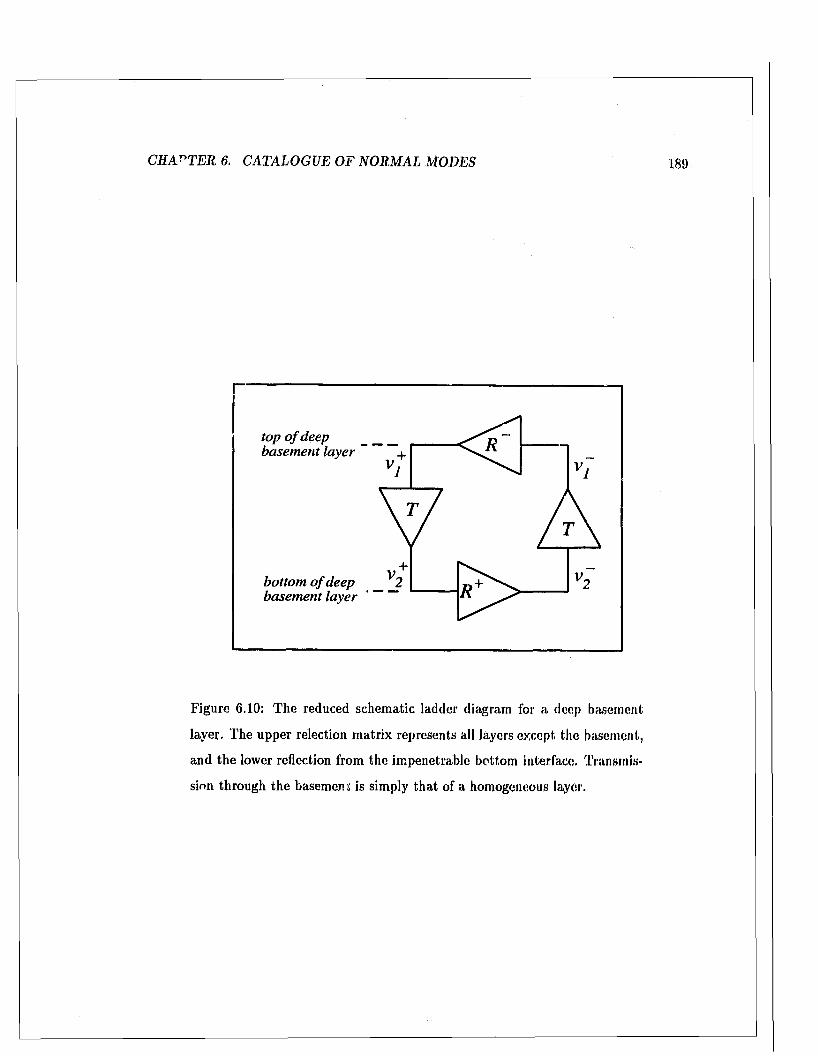
C H A P T E R 6. C A TA LO G U E OF N O R M A L M O D ES 189
top o f deep basem ent layer
bottom o f deep basem ent layer
Figure 6.10: T he reduced schem atic ladder diagram for a deep basement
layer. The upper relection m atrix represents all layers except the basement,
and the lower reflection from the im penetrable bottom interface. Transmis
sion through the basemen s is simply th a t of a homogeneous layer.
C H A P TE R 6. C ATA LO G U E OF N O R M A L M ODES 190
6.4.2 The spacing of radiation m odes
Since H is large, the phase term s change considerably over a small step
Ac/ along a. branch line, whereas the reflection m atrix components Rfj change very little. If
a radiation mode exists a t some value of q, neighboring modes should lie along the branch
line at r/ ± A q where
2u>A qH m 2n. (6.19)
Using A q « (dq/dp ) A p = - (p/q) Ap, the estim ate of the m ode spacing along a branch line
is
<«■»The estim ate improves as 11 is made larger.
Notice th a t the modes can be very close together near the branch point where
q m 0. By analogy with the elem entary oceanic waveguide, let us assume th a t the first
radiation mode on a branch line—the mode closest to the branch point—occurs when a
quarter P or S Wavelength A fits vertically inside the basem ent layer
H * I - 7 h (6-21)
Furtherm ore, assuming th a t p « 1/c near the branch point, the estim ated mode spacing
(6.20) gives
A p K ~ 8 ] h ~2 (6-22)
near the branch point, where c = a or /? according to the branch line. T he search resolution
needed to resolve radiation modes near the branch point m ust be somewhat smaller than
this.
Radiation modes are further ap art away from the branch point. T he largest Ap
occurs near p — 0, a t the knee in the E JP branch line. In fact, the estim ate (6.20) may
break down a t the knee because it assumes A p is small. Following the E JP branch line high
along the positive im aginary axis, however, q = s / l /c * - p2 -> p, and the mode spacing
approaches a constant independent of the elastic media
Ap ~ 2 j H ' ^ '23)
C H A P T E R 6. C ATA LO G U E OF N O R M A L M ODES 191
The radiation modes trail indefinitely along the imaginary axis with roughly this spacing.
This result also applies for high-order evanescent plate modes which m ight be viewed as a
special case of radiation modes trapped in a distinct plate-like structure.
6.4.3 E stim ating the number o f radiation modes
Let us estim ate the num ber of propagating radiation modes dose to the real p axis,
along the horizontal portion of the branch line. For simplicity, neglect the small imaginary
part of the phase speed c (a or /?), then the branch line follows the real slowness axis from
p = 1 /c to 0, where q — 0 and 1/c , respectively. For waves travelling the circuit from top to
bottom to top again in the basem ent layer, the change in vertical phase along this horizontal
part of the branch line (ignoring changes in Rfj in (G.18)), is roughly 2u> A q l f as 2u> II/<•.
Dividing this to tal change of phase into 2 k steps gives an estim ate of the minimum number
of propagating radiation modes for one branch line
N v « ^ = 2f H / c s= 2 // /A ; (6.24)2 k c
A being the wavelength of P or S waves in the bottom , depending on which branch line
is under consideration. Notice there are proportionally fewer propagating modes at low
frequencies than a t high because the m ode spacing is inversely proportional to frequency
( 6 .20).
Applying the estim ate to the two-layer oceanic model considered earlier in C hapter
6, Table(6.3), we have
I I 1500 m,
A« = a / / = 3000./100 = 30.00 m, (0.25)
\ p - f i / f = 1732./100 = 17.32 m;
henceN p as 100 P-wavc radiation modes,
N p as 173 S-wave radiation modes, (6.20)
Total = 275
which compares well w ith the total of 255 radiation modes actually found near the horizontal
branch lines in Fig. (6.7), in the range 0 < pT < 1/1732 = 0.577 s/km , and 0 < p t < 0.02
C H A P T E R 6. C ATA LO G U E OF N O R M A L M O O ES 192
s/km .
Applying the estim ate to a m ore realistic model, the Arctic waveguide considered
earlier in Table (5.1), we have
I I = 2000 m,
= a / f = 5250/20 = 262.5 m , (6.27)
A/j: = / ? / / = 2500/20 = 125.0 m;
henceN p 15 P-wave radiation modes,
N p « 32 S-wave radiation modes, (6.28)
Total = 47
which compares well with the to ta l of 45 radiation modes actually found near the horizontal
branch lines in Fig. (5.6),
I t is im portant to know roughly how m any evanescent radiation modes m ay be
required to com pute the field in the bounded waveguide to a specified relative precision e.
To this end, let us assume, as in the convergence tes t (5.42), th a t the radiation m ode series
has converged when
» — £ $ • <6-29>Dividing by the m agnitude of the asym ptotic spacing (6.23) gives the num ber of evanescent
modes
N e « (6,30)7r r
A t small ranges the num ber of modes m ay be prohibitively large. A t very large ranges, no
evanescent modes m ay be required. Unlike the propagating modes, the num ber of evanescent
radiation inodes N c needed a t close ranges is independent of frequency because both the
maximum im aginary slowness spanned by the significant evanescent modes (6.29), and the
asym ptotic mode spacing, are inversely proportional to frequency.
6 .4 4 Correspondence w ith the unbounded waveguide
Radiation modes of the bounded waveguide presum ably approxim ate the contribu
tion of the branch line integrals of the unbounded, Frisk dem onstrates the correspondence
C H A P T E R 6. C ATA LO G U E OF N O R M A L M OD ES 193
for a two-layer fluid (Pekeris) waveguide [48]. The extension to elastic m edia will not be
attem pted here, except to point out th a t the branch line mode spacing (6.20) vanishes as
H oo, as it m ust if the serie-' e'-o.nes an integral in the limit; and th a t the Held for
each rad iation m ode can be w ritten in term s of down and up going waves in the basement
layer, as it m ust if the series represents the integral along bo th sides of the EJ P branch cut
simultaneously.
For modeling purposes, it is im portant to know when tiie deep bounded waveguide
accurately models the unbounded case. One rule of thum b can be derived by viewing the
branch line m ode series as a numerical approxim ation to the branch line integrals. Obviously
the modes cannot be too far apart or the integrand will not; be adequately sampled along
the branch line. Indeed, there should only be a small change in the complex phase c!i°1>r
between modes
w |Re{Ap}| r < 2it. (6.31)
Assuming a lossless bottom medium, Ap is pure real along the E JP branch line from the
branch po in t to the origin, and using (6.20), (6.31) becomes
577 < « u 2 >
where p' is the slowness of the mode closest to the origin where |Ap| is maximal. This limit
has a physical in terpretation, for equality of both sides in (6.32) is the. condition of the. first
bottom bounce of “rays” having horizontal and vertical slowness, p' and q'. And as the
range from the source increases from zero, it is the bottom reflections of the mode with the
moot vertically directed rays— the mode at the knee of the branch line th a t first ruins the
correspondence between the unbounded and deep bounded waveguides, as we might have
expected.
Unfortunately, p' for the mode a t the knee of the branch line cannot be estim ated
in a general way, and the limit on r can only be estim ated once the mode lots been found.
Nevertheless, it is reasonable to take q' = \ J l / (P‘ - { p ' f « 1/c since p' lies near the origin,
where |A p| is a m axim um , so th a t (6,32) simplifles to
r < 2 tlp'c, (6.33)
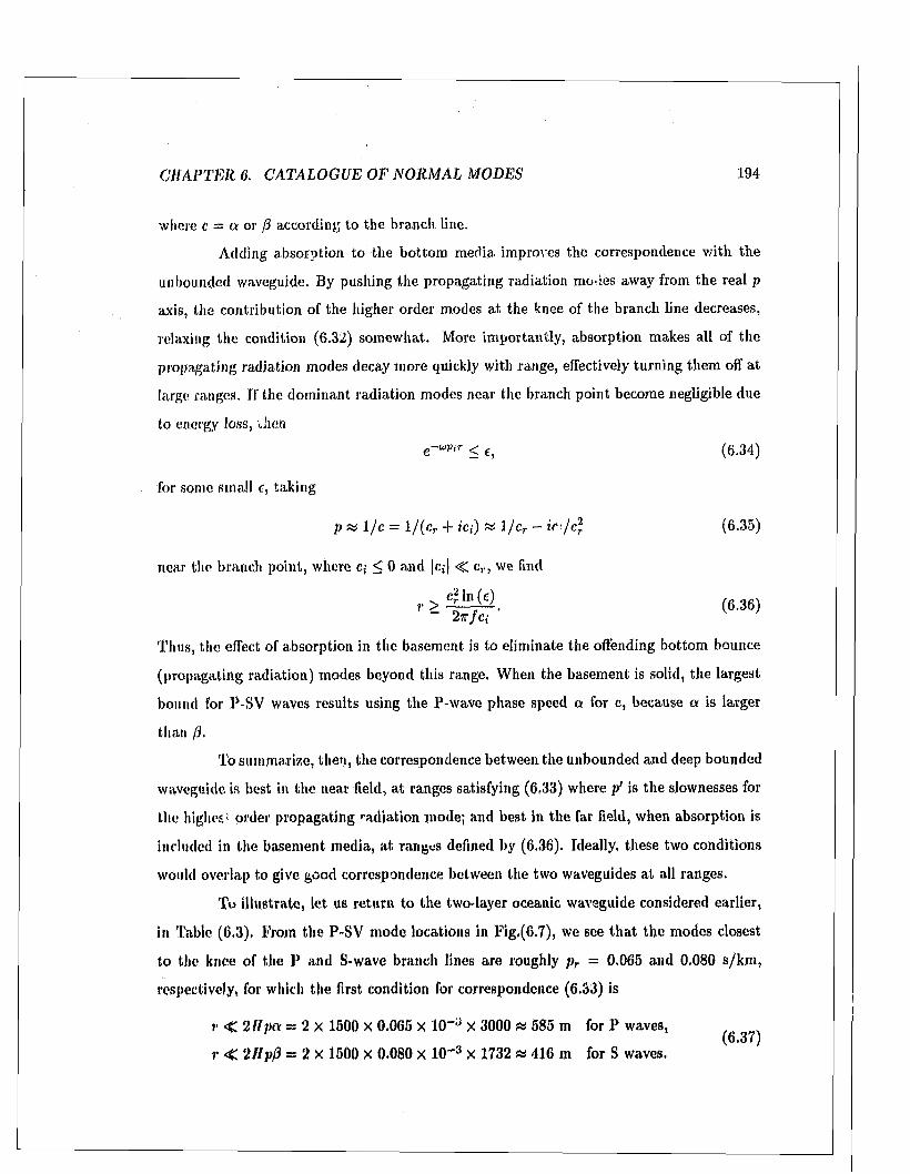
C H A P T E R 6. C ATA LO G U E OF N O R M A L M OD ES 194
where c = a or ft according to the branch line.
Adding absorption to the bottom m edia improves the correspondence w ith the
unbounded waveguide. By pushing the propagating radiation modes away from the real p
axis, the contribution of the higher order modes a t the knee of the branch line decreases,
relaxing the condition (6.32) somewhat. More im portantly, absorption makes all of the
propagating radiation modes decay m ore quickly with range, effectively tu rning them off at
large ranges. If the dom inant radiation modes near the branch point become negligible due
to energy loss, Jicn
e~up,T < c, (6.34)
for some small <r, taking
p m 1/c = l / ( c r + ici) ta \Jcr - (6.35)
near the branch point, where c; < 0 and |c,| < cr , we find
r > (6-36)2tt j C{
Thus, the effect of absorption in the basement is to elim inate the offending bottom bounce
(propagating radiation) modes beyond this range. W hen the basement is solid, the largest
bound for P-SV waves results using the P-wave phase speed a for c, because a is larger
than ft.
To summarize, then, the correspondence between the unbounded and deep bounded
waveguide is best in the neat field, a t ranges satisfying (6,33) where p' is the slownesses for
the h ig h er order propagating radiation mode; and best in the far field, when absorption is
included in the basement media, a t ranges defined by (6.36). Ideally, these two conditions
would overlap to give good correspondence between the two waveguides a t all ranges.
To illustrate, le t us return to the two-layer oceanic waveguide considered earlier,
in Table (6.3), From the P-SV m ode locations in Fig,(6.7), we see th a t the modes closest
to the knee of the P and S-wave branch lines are roughly pr = 0.065 and 0.080 s/km ,
respectively, for which the first condition for correspondence (6.33) is
r < 2 H pa ~ 2 X 1500 X 0.065 X 10";J X 3000 » 585 m for P waves, ^
r < 2Hpfl — 2 X 1500 X 0.080 x 10"3 X 1732 « 416 m for S waves.
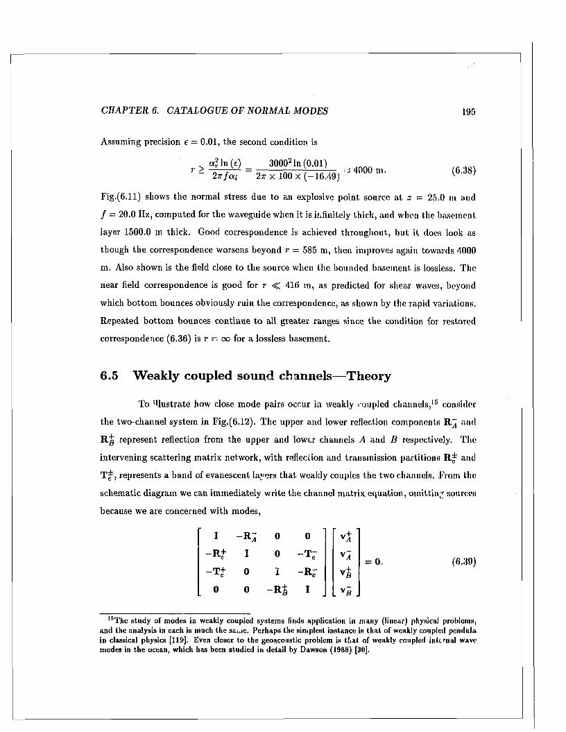
C H A P T E R 6. C ATA LO G U E OF N O R M A L M ODES 195
Assuming precision e — 0.01, the second condition is
- a? In (e) 30002ln (0.01)r > 0 ’ = -z------ t 4000 m,2-Kjai 2x x 100 x (-16 .49) (6.38)
Fig.(6.11) shows the normal stress due to an explosive point source at z — 25.0 m and
/ = 20.0 Hz, com puted for the waveguide when it is infinitely thick, and when the basement
layer 1500.0 m thick. Good correspondence is achieved throughout, but it does look as
though the correspondence worsens beyond r = 585 m, then improves again towards 4000
m. Also shown is the field close to the source when the bounded basement is lossless. The
near field correspondence is good for r -C 416 m, as predicted for shear waves, beyond
which bottom bounces obviously ruin the correspondence, as shown by the rapid variations.
R epeated bottom bounces continue to all greater ranges since the condition for restored
correspondence (6.36) is r - oo for a lossless basement.
6.5 W eakly coupled sound channels— T heory
To ;Uustrate how close mode pairs occur in weakly coupled channels,15 consider
the two-channel system in Fig.(6.12). The upper and lower reflection components R)J and
R g represent reflection from the upper and lower channels A and B respectively. The
intervening scattering m atrix network, with reflection and transmission partitions R * and
T f , represents a band of evanescent layers tha t weakly couples the two channels. From the
schematic diagram we can immediately write the channel m atrix equation, om itting sources
because we are concerned with modes,
I - * A 0
- K t I 0
"T+ 0 I
0 0 -R fl
- T “X C
-R 7
■< M
- !
1 ^
>
VB
. VB .
= 0 . (6.39)
15The study of modes in weakly coupled system s finds application in many (linear) physical problems, and the analysis in each is much the sa.ae. Perhaps the simplest instance is th a t of weakly coupled pendula in classical physics [119]. Even closer to the geoacoustic problem is th a t o f weakly coupled internal wave modes in th e ocean, which has been studied in detail by Dawson (1988) [80].
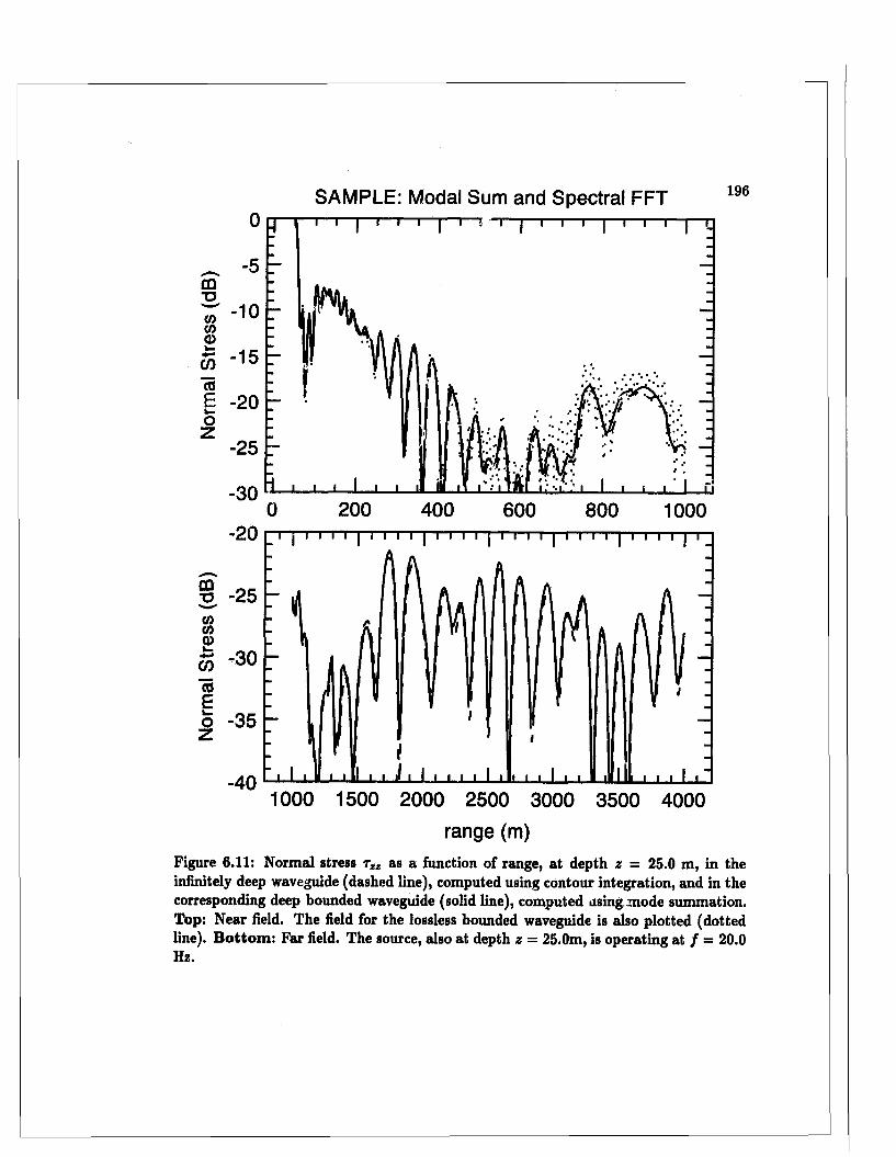
SAMPLE: Modal Sum and Spectral FFT0
5
■o-10
-15
E -20
-25
-300 200 400 600 800 1000
-20
-30
o -35
-401000 1500 2000 2500 3000 3500 4000
range (m)Figure 6.11: Normal stress t xz as a function of range, at depth z = 25.0 m, in the infinitely deep waveguide (dashed line), computed using contour integration, and in the corresponding deep bounded waveguide (solid line), computed using, mode summation. Top: Near field. The field for the lossless bounded waveguide is also plotted (dotted line). B ottom : Far field. The source, also at depth z = 25.0m, is operating at / = 20.0 Hz.
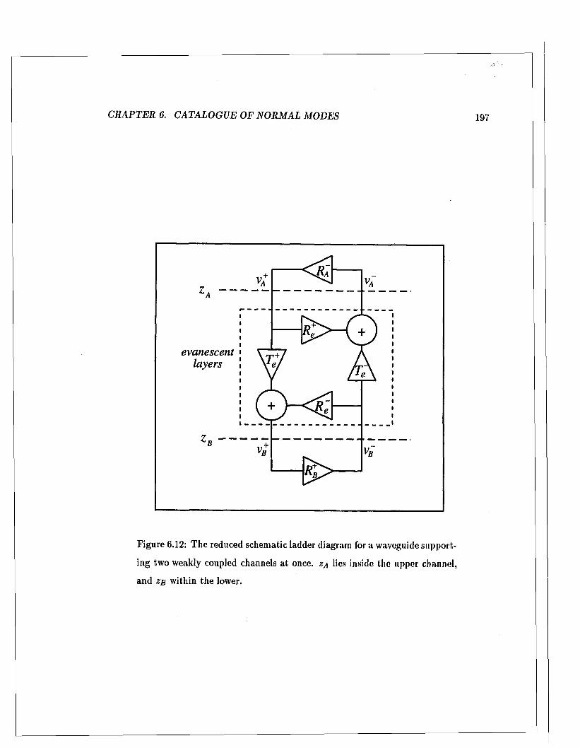
C H A P TE R 6. C ATA LO G U E OF N O R M A L M ODES 197
evanescentlayers
Figure 6.12: T he reduced schematic ladder diagram for a waveguide support
ing two weakly coupled channels a t once, za lies inside the upper channel,
and zb within the lower.
C H A P TER 6. C A TA LO G U E O F N O R M A L M OD ES 198
The decoupling of channels is evident when the transm ission T f goes to zero due
to strong vertical evanescence. A t the sam e time, the determ inant of the m atrix goes to
I - R ^ I - R g -
- R + I - R + I- e = | I - R ^ R + | . | l - R - R + | - 6 , (6.40)
where e = e(uj,p) is a small num ber whose m agnitude is less th an some upper bound given
by
M < C ||T + || ||T e- | , (6.41)
where C is a positive real constant and ||T ^ || denotes a norm of the transm ission m atrices.
In the scalar case for P waves, for example, when za and zb lie in fluid layers, the reflection,
transmission, and identity partitions in (6.39) are all scalars, giving
|e| = |R ^R +| |T + | |T - | (6.42)
In the lim it of to ta l decoupling ||T ^ || —► 0, hence e —> 0, and the condition for a m ode—th a t
(6.40) be zero—becomes
| I - R ^ R + | . | l - R - R + | = e * 0. (6.43)
A t a mode, either
| I - R J R f | « 0 , (m 4 )
|I — R e R g j « 0,
or both determ inants are simultaneously small. These determ inants are the characteristic
equations for m odes in each channel considered separately, so the modes of the weakly
coupled channels are located near the modes of each channel considered independently, as
expected.
Close m ode pairs occur when both conditions (6.14) are satisfied simultaneously.
The slowness p and frequency u> of the modes m ust be a point on the dispersion curves
where the curves for each channel would cross if the channels were totally decoupled. In
the vicinity of such a crossing point pc, the left sides of (6.44) can be approxim ated by a
Taylor series expansion
|I - R ^ R + | = 0 + \ A ( P -P c ) + 0 ((p - pc)2) ,
| l - R “ R £ | = 0 + A b(p — Pc) + O ((p - p c)2) ,(6.45)
C H A P TE R 6. C A TA LO G U E OF N O R M A L M OD ES 199
where A^ and Ab are the first derivatives of the left sides of (6.44) evaluated at pc.w Sub
stituting these into (6.43) and retaining only the first order term s, gives the characteristic
equation for the weakly coupled channels near the crossing point pc
A^Ab (p - pcf = e.
Solving for p, we find a pair of modes for the coupled system
p = pc ± \J cI \ a Xb = Pc ± A p/2 .
(6.46)
(6.47)
The spacing between a mode pair |Ap| = 2 Jv^/A^Ab] can be very small indeed since e —> 0
exponentially due to vertical evanescence. An extensive search at the resolution needed to
distinguish the pair would usually not be feasible, bu t they can be identified and resolved
using the singular values of the channel m atrix during the mode search function as described
in Section (5.3.3).
T he mode functions for a close mode pair are approxim ately anti-sym m etric, just
as the modes for th e classic m ode problem for weakly coupled pendula are anti-sym m etric
[23]
(6,48)
Thus, both modes m ust be alm ost equally excited when the source lies in ju st one channel to
achieve cancellation in the o ther channel. B ut at large distances from the source, the slightly
different horizontal slownesses for a m ode pair causes the m ode functions to interfere (beat)
with each other. Assuming a range phase dependence eiupr characteristic of cylindrical
waves in the far field, for example, the sum of the two equally excited modes can be written
1
>1 ______
i
>■ 1
>■
0o r
0
V B 0 0
. V S . . v i . 11 < CD 1
I— ■
16Here I have assumed th a t \ a and Ab are no t zero, which could only occur if the mode in cither system was itself a double (or higher) mode, meaning th a t there arc actually three or more resonant modes at slowness p—a very unlikely situation in naturally occuring waveguides.
C H A P T E R 6. C ATA LO G U E O F N O R M A L M O D ES 200
as
2v+ ejupcr cog L.:& pr/2
0
0
2 i V g e twpcT s m u > A p r / 2
(6.49)
The interference causes the sound energy of bo th modes together to transfer between the
channels over a cycle distance D = 2w/(u> Re {Ap}) = ( /R e { A p })_1 in range. The sit
uation is analogous to the transfer of pendulum m otion in the coupled pendula problem.
Motion in ju s t one pendulum is in tim e transferred to its resonant partner, originally s ta
tionary, then back again, and so repeatedly transferring the vibration energy between the
two pendula W hat happens in tim e between resonant pendula, happens in range between
resonant channels in the waveguide: waves travelling in one channel are over long distances
transferred to the other, and the back again, w ith cycle distance D.
To illustrate, consider the almost sym m etric fluid waveguide in Table (6.5), con
trived for dem onstration of weakly coupled resonant modes. Fig. (6.13) shows the first and
second singular values in the search for propagating modes along the real axis a t 12 Hz.
Close to a mode pair, the search functions follow the form described earlier in Fig. (5.4),
which is evident for the second pair (modes 3 and 4, spacing Ap = .003475 s/k m ), though
not for the first pair (1 and 2, spacing Ap = .0002484 s/km ) a t the scale of the figure. The
antisym m etric nature of the vertical mode functions is evident in the bo ttom figure. Fig.
(6.14) shows the transfer of sound energy between the two channels with range for modes 3
and 4 alone. The source is an explosive point source (12 Hz) in the upper channel a t z = 50
m.
Resonant sound channels m ay be encountered occasionally when m odeling waves
of one frequency in a range independent waveguide. In practice, the frequency band of an
acoustic signal may span several resonances, and slowly varying layer thicknesses and elastic
properties m ay cause channels to tune in and o u t of resonance as the sound propagates,
making the coupled channels much more likely, possibly resulting in a partia l transfer of
energy between weakly coupled channels, though w ithout ongoing repetition.
eiu/(pc+Ap/2)r
i<
0 _j_ eio>(pm-Ap/2)r 0 _0 0
\---- < to t
i___
. ~ VB .
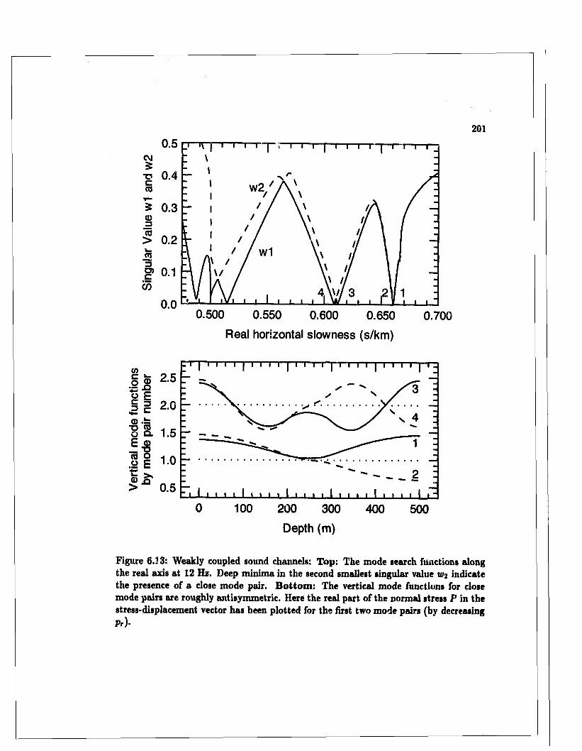
2010.5
CM5
t? 0.4cco
i 0.3 o>
> 0.2
w2
w1L_«3O)c
CO0.1
0.00.500 0.550 0.600 0.650 0.700
Real horizontal slowness (s/km)
V)co 2.5oc3 2.0 d) ~13 2. 1.5
- fS | 1 - 0c > ,
> 0.50 100 200 300 400 500
Depth (m)
Figure 6.13: Weakly coupled sound channels: Top: The mode search functions along the real axis at 12 Hz. Deep minima in the second smallest singular value u>2 indicate the presence of a close mode pair. B ottom : The vertical mode functions for close mode pairs are roughly antisymmetric. Here the real part of the normal stress P in the stress-displacement vector has been plotted for the first two mode pairs (by decreasingP r) .
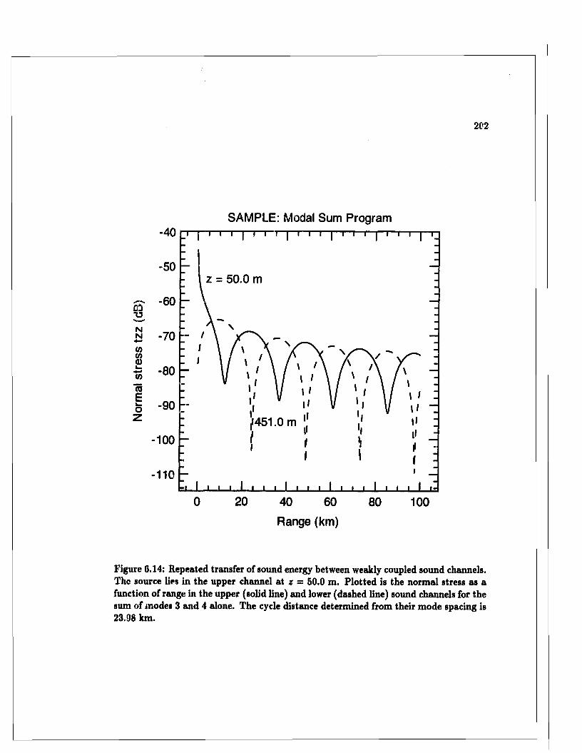
SAMPLE: Modal Sum Program-4 0
-5 0z = 5 0 .0 m
s * -6 0CDTONN4— -7 0OT(/>a)U.
-8 0wcoE
- 9 0v—oz i>4 5 1 .0 m
-100
-110
200 4 0 6 0 8 0 100Range (km)
Figure 6.14: Repeated transfer of sound energy between weakly coupled sound channels. The source lies in the upper channel at z = 50.0 m. Plotted is the normal stress as a function of range in the upper (solid line) and lower (dashed line) sound channels for the sum of modes 3 and 4 alone. The cycle distance determined from their mode spacing is 23.98 km.

C H A P T E R 6. C ATA LO G U E O F NORMAL M ODES 203
z zlayer upper lower a P pno. (m) (m) (m /s) (m /s) (kg /m 3)1 0.0 200.0 1500.0 0.0 1000.2 200.0 300.0 2000.0 0.0 1000.3 300.0 501.0 1500.0 0.0 1000.
Table 6.5: Almost sym m etric fluid waveguide. The top and bottom of the
waveguide are bounded by a rigid plane.
204
C h a p t e r 7
BIE m ethod for layered m edia
I have so far developed a, new indirect B IE m ethod for the scattering of elastic waves
and a norm al mode m ethod for numerically com puting the complete G reen’s function for
layered media. It remains to unite them in a single model of elastic wave scattering. This is
a straightforw ard task from a program m er’s perspective, for we need only make the modal
summation subroutine available to the existing G reen’s function subroutine. The m atter
is much m ore complicated from the user’s perspective, for, as we will see, one p a rt of the
scattering problem cannot be freely specified w ithout regard for another since there are
several com peting param eters th a t m ust be balanced for the model to run successfully. As
in BIE m ethods generally, the kinds of problems th a t can be solved are biased towards low
frequency scattering, for the wavelength cannot be too small compared to the dimensions
of the inclusion or the num ber of elements needed to represent its boundary will exceed a
practical lim it. In layered m edia, when using m ode sum m ation for the G reen’s function,
the low-frequency bias appears in another way, for the wavelength cannot be too small
compared to the thickness of the waveguide or there will be a proliferation of significant
modes beyond a practical lim it. These constraints are reviewed below.
7.0.1 Constraints due to elem ent size
We have seen th a t the size of the boundary elements m ust be small compared
to the wavelengths in their vicinity. Frequency and phase speed therefore constrain the
C H A P T E R 7. B IE M ETH O D FO R L A Y E R E D M ED IA 205
maxim um size of the elements, which in tu rn determines the minimum num ber of elements
needed to cover a given scattering inclusion. On the other hand, lim itations ou the available
com puter memory and execution time place a maximum lim it on the number of boundary
elements, because increasing the num ber of elements increases the num ber of nodes, which
in tu rn increases the num ber of unknowns and equations in the dense partitions of the DIE
coefficient m atrix. Both constraints m ust be satisfied to solve a scattering problem. Similar
constraints apply in almost all numerical scattering models, whether or not BIE m ethod is
used or layered m edia are included.
W hen specifying the element size, both the P and S wavelengths must be consid
ered. Sea floor sediments pose particular difficulty since the S wave speeds in the upper
sediment layers can be very small, perhaps 200 to 300 m /s , whereas the P wave speed may
be somewhat higher than th a t of water, 1500 m /s. This makes the P wavelength roughly
7.5 times larger th an the S. In scattering from a sphere, for example, when hr = 3.0 lor
P waves, it may be 22.5 for S, which is ra ther large for any three-dimensional lull-wave
model to handle. Thus, low speed sediments can only be included in the waveguide if the
scattering inclusion does not pass through them.
Finally, tall vertical sides to the scattering inclusion should be avoided in the
indirect B IE m ethod for layered media, because the integral coefficients lor all elements
above and below a surface com putation point are troublesome due to poor convergence in
the mode series, whereas perhaps only as many as six troublesome elements can be handled
reliably.1 Hence, a vertical side wall cannot be much greater than the smallest wavelength
near the inclusion.
7.0.2 Constraints due to m ode proliferation
We have seen th a t a complete norm al mode treatm ent of the G reen’s function is
only possible for waveguides th a t are bounded top and bottom by an im penetrable , 1
boundaries. Moreover, as the bounded waveguide is made thicker, or frequency is increased,
there is a proliferation of radiation modes th a t must be included in the mode series,2 which
‘The indirect method becomes numerically unstable as the num ber of troublesom e elem ents in an equation increases; see Section (3.5.1).
2See Section (6,2,2).
04
C H A P T E R 7. B IE M ETH O D F O R L A Y E R E D M ED IA 206
can make the mode search tedious, and the m odal sum m ation intolerably slow. T he rules
for estim ating the num ber of propagating and evanescent radiation modes in term s of the
frequency and waveguide thickness are given in Section (6.4). It m ust be rem em bered th a t
there m ay be more than one evanescent mode series, since each plaie-like structu re in the
waveguide is likely to have its own plate modes trailing along both sides of the imaginary
slowness axis. Fortunately, the vertical mode functions of evanescent plate modes are con
fined within the plate-like structure th a t engenders them , so entire series of evanescent plate
modes can be om itted if the scattering inclusion lies outside the plate.
7.1 T h e particular so lu tions for layered m edia
I t is im portan t to note th a t, unlike homogeneous domains, the point sources gen
erating th e particular solutions in layered m edia cannot lie w ithin, or directly above or
below the scattering inclusions, again because of poor convergence in the mode series when
com puting the particular solution (unscattered incident field) a t the boundary. To accom
m odate those source locations, while still using a truncated mode series, we would have
to derive a new delta-function sifting term £ for the incident field te rm ,3 by excluding the
source using a vanishingly small exclusion cylinder, positioned vertically, reaching from the
top to the bottom of the waveguide and piercing through the scattering inclusion. Although
I have had some success along these lines, I have nothing conclusive a t the time of writing.
I t is best to use particular solutions th a t excite both P-SV and SII waves (in solid
layers) in significant proportions, to provide as much inform ation to the indirect solution as
possible. This can be done in layered m edia by exciting b o th a horizontal tw isting source
plus a random ized point force. The horizontal tw isting source is a source of SH waves tha t
can be im agined as horizontal ro tational oscillations of a point in welded contact about its
vertical axis. If. consists of a m om ent tensor in (4.54) having the form
M =
J M n 0
- M u 0 0
0 0 0
(7.1)
aSee Scction(2.4),
C H A P T E R 7. B IE M ETH O D FO R L A Y E R E D M ED IA 207
7.2 Interfaces and edges
W e have seen th a t the displacement tangential to an interface with a fluid can be
discontinuous. W hen the boundary of the scattering inclusion is smooth and passes through
the plane interface adjoining a fluid layer, the component of displacement tangential to both
the plane interface and the inclusion boundary (the horizontal component of displacement
tangential to the boundary) can therefore be discontinuous as well. To perm it a displace
ment discontinuity, we can trea t the line of contact between the interface and boundary
using double nodes along the line [8, sect. 7.2.3]. To place nodes on this line of disconti
nuity, it m ust be a dividing line between boundary elements. And to place double nodes
on the line, the nodes from elements on both sides of the line must be treated as separate
nodes, even if they are coincident. Coupling of the field can be enforced between double
nodes using additional coupling equations in the coefficient m atrix (3.8) th a t relate double
nodes in the same perspective. For instance, assuming th a t the interface between a fluid
and solid layer lies outside the boundary, the continuity equations between double nodes
would equate the traction vector, the vertical displacement, and the horizontal displacement
normal to the boundary, while leaving the horizontal component of the tangential displace
ment discontinuous. If there is an interface both outside and inside the boundary, however,
as there will be in th e free-field test in layered domains, the continuity of the horizontal
displacement norm al to the line of discontinuity should not be enforced.
T he traction vector will be discontinuous across an edge in the boundary, because
the traction depends on the norm al vector, The discont: nuity in traction can also be handled
using double nodes and additional coupling equations. Here again, the coupling conditions
depend on the media, whether fluid or solid, both inside and outside the scattering inclusion.
M atters become ra ther complicated if an edge is coincident with an interface between a fluid
and solid layer.
I will not a ttem p t a general treatm ent of lines of discontinuity here. When in
doubt, it seems the best policy is to enforce no coupling between double nodes and let
the BIE solution resolve discontinuities itself. Instead of using coincident double nodes,
for example, we could stagger the nodes across the line of discontinuity, in which case, no
C H A P T E R 7. B IE M ETH O D F O R L A Y E R E D M ED IA 208
coupling is the only possibility, The worst policy is to force continuity where it should
not be, for, like the error of welded contact with fluids (Section (2.3.2) and (3.2.4)), it
forces the BIE m ethod to solve the wrong—if not a meaningless— boundary value problem.
Examples of edges and extension of the inclusion through a fluid-solid interface are among
the dem onstrations given below.
7.3 D em onstration o f th e BIE m ethod for layered m edia
After a particular scattering problem has been carefully planned, and i t has been
determined th a t the num ber of modes and boundary elements are practicable, the new
model proceeds in this way:
1. the modes m ust be found, and their vertical m ode functions computed;
2. the source locations for the particu lar solutions, and their fields u and t a t the bound
ary element nodes m ust be com puted and saved for quick access;
3. the surface- and null-fleld com putation points m ust be chosen, and the coefficients
for their corresponding integral equations com puted (using the particular solutions to
com pute troublesome coefficients indirectly) and verified using consistency tests and
the free-field test;
4. the integral equations, together with the boundary and continuity conditions, m ust
be solved for u and t a t the boundary nodes, then verified using th e null-fleld test;
5. the displacement u can be com puted a t points off the boundary using the whole-field
equation .'1
I t need hardly be mentioned th a t the new model, like m ost three-dim ensional
models of scattering, requires considerable time and effort to setup and run, especially
in its earliest stages of development. It also requires m any utility programs to specify
the boundary elem ents, autom atically choose points of one kind or another, verify test
'Components of the stress tensor r could also be computed as noted in Section (3.2.5).

C H A P T E R 7. B IE M ETH O D F O R L A Y E R E D M ED IA 209
results, and plot the boundary and elastic field. It is impossible to review all of this in
detail. Instead, my aim is to show th a t the m ethod works in elastic waveguides, and to
indicate th e diverse range of problems it can undertake, such as scattering from penetrable,
im penetrable, and mixed inclusions th a t cross a layer interface.
To dem onstrate th a t a model works is one task, bu t to analyze the corresponding
physics is quite another. At this early stage in the model development, I will not venture,
far into th e analysis of scattering, by hypothesizing general rules governing scattering in
such cases for example, for th a t requires considerably more detail than a dem onstration
requires, plus m any more simulations for verification. W ithout knowing beforehand what
direction such rules about scattering m ay take, I hope the dem onstrations will be complete
enough to allow readers (and myself a t a la ter date) to make prelim inary judgm ents about,
scattering, or to find confirmation of principles derived in o ther ways.
Three dem onstrations will be given, ordered by increasing complexity; they are
scattering by 1) a cavity in an ice plate, 2) a half-buried sphere on the sea floor in a shallow
ocean, and 3) a circular ice dome in a floating ice plate in an Arctic environment.
7.3.1 Hem ispherical cavity in an ice plate
To begin, let us consider scattering from a i m radius hemispherical cavity on
the floor of a 3 m free ice plate. For simplicity, the ice, frequency (750 Hz) and modes
are the sam e as for the free p late considered earlier in Fig. (6.1). Details of the HIE
setup are summarized in Table (7.1). Twenty boundary elements cover the hemisphere as
shown in Fig. (7.1). T he sources generating particular solutions for the indirect coefficient
com putations are positioned as shown in Fig. (7.2), the excitation for each source being
the sum of a randomly oriented point force and horizontal tw isting source (7.1). More than
enough modes have been found as shown in Fig. (7.3), where the relative strength of each
mode has been plo tted , when evaluated a t the edge of the close neighborhood in which
indirect com putations are performed.
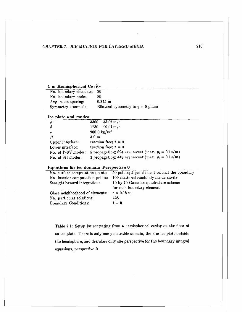
C H A P T E R 7. B IE M ETH O D F O R L A Y E R E D M ED IA 210
1 m Hemispherical CavityNo. boundary elements: 20No. boundary nodes: 89Avg. node spacing: 0.375 mSymmetry assumed: Bilateral sym m etry in y = 0 plane
Ice plate and modesaftoIIUpper interface- Lower interface:No. of P-SV modes: No. of SH modes:
3300 - 33.0« m /s 1730 - 20.0? m /s900.0 kg /m 33.0 mtraction free; t = 0 traction free; t = 05 propagating; 894 evansecent (max. pi = 0.1 s / m ) 3 propagating; 448 evansecent (m ax. pi = 0.1 s / m )
Equations for ice domain: Perspective 0No. surface com putation points: No. interior com putation points: Straightforw ard integration:
Close neighborhood of elements: No. particu lar solutions: Boundary Conditions:
50 points; 5 per element on half the boundary100 scattered random ly inside cavity10 by 10 Gaussian quadrature schemefor each boundary elementc = 0.15 m428t = 0
Table 7.1: Setup for scattering from a hemispherical cavity on the floor of
an ice plate. There is only one penetrable domain, the 3 m Ice p late outside
the hem isphere, and therefore only one perspective for the boundary integral
equations, perspective 0.
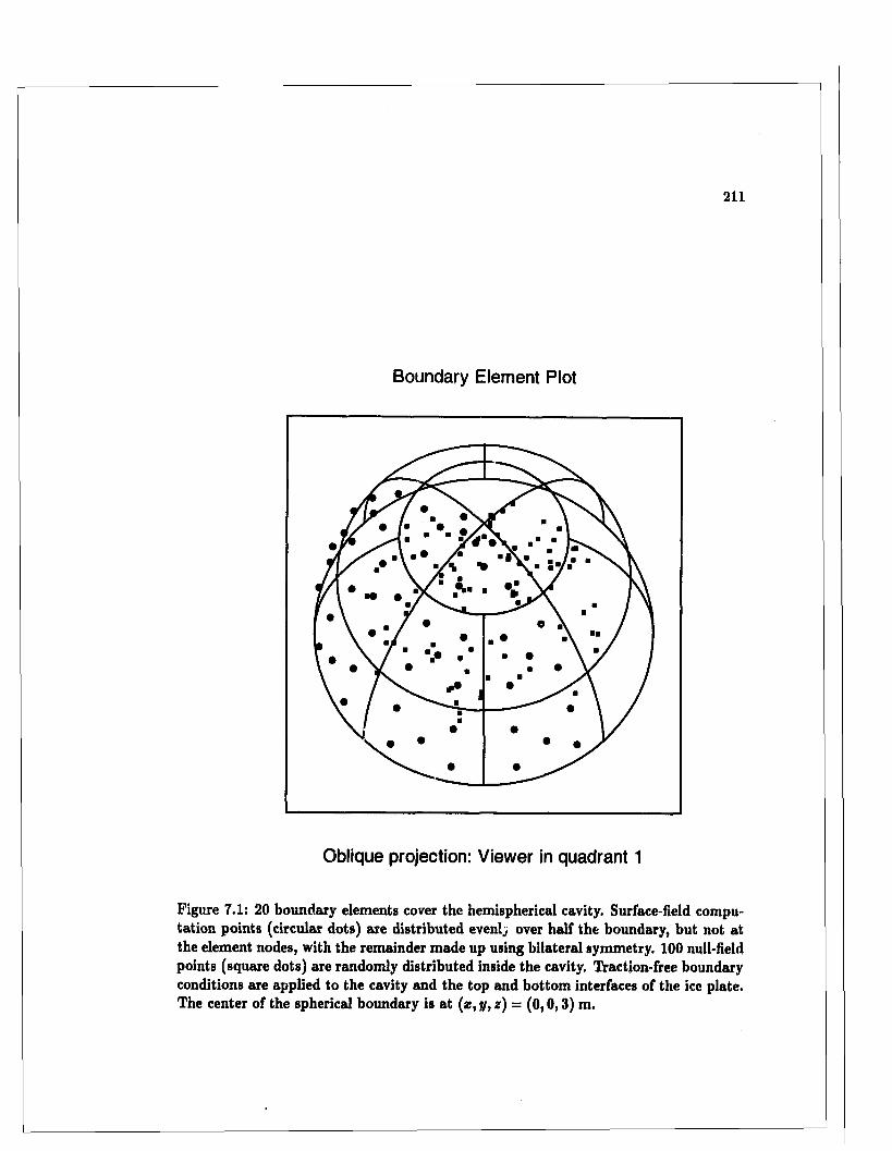
211
Boundary Element Plot
■■
Oblique projection: Viewer in quadrant 1
Figure 7.1: 20 boundary elements cover the hemispherical cavity. Surface-field computation points (circular dots) are distributed evenly over half the boundary, but not at the element nodes, with the remainder made up using bilateral symmetry. 100 null-field points (square dots) are randomly distributed inside the cavity. Traction-free boundary conditions tire applied to the cavity and the top and bottom interfaces of the ice plate. The center of the spherical boundary is at (z, y, z) = (0,0,3) m.
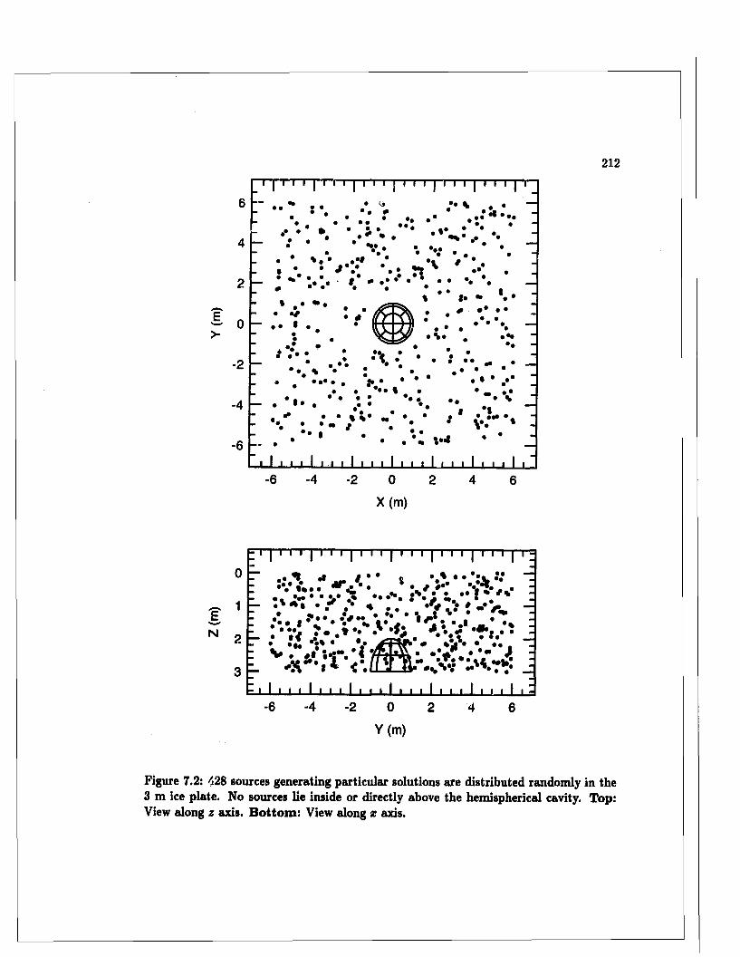
E,>
6
4
2
0
-2
-4
-6
- • „ • • • g i* • •# a
I vi* • - -: . • ...~v •.? • :• \ * * •*. • : Tt •• • -
— _: *, .V ’ ■• • * : • '• • • •
• ••
>• • *•- %
•
* . * • /• • • • I •• , • • • • '• « • • • • • * •
• •
• • % M• - ; . t
• ■ • • • '
»•«*
i I ' i i I ' i • I » i ' I i i ■ I i i i I i i i I-6 -4 -2 0
X (m )6
212
EN
: I | I I I | I I I | I I I |
Figure 7.2: 428 sources generating particular solutions are distributed randomly in the 3 m ice plate. No sources lie inside or directly above the hemispherical cavity. Top: View along z axis. B ottom : View along x axis.
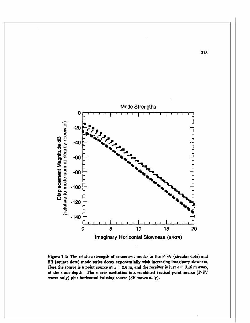
213
0 — i— i— rMode Strengths
t— i— i— i— i— i— i— i— i— i— i— i— i— r
(1)>'55
CD 8■o *-
I *1 = « to
c Ia) to E ®8 32 E«" 2D <D
>i !d)
- 2 0 ' ’ . r -i r •• ■■ \ .7ji— 1 . • J
*-40
-60
-80
■100
■120
■140J I I i 1 i i i I I I I I ... 1 J I 1 I L
0 5 10 15 20Imaginary Horizontal Slowness (s/km)
Figure 7.3: The relative strength of evanescent modes in the P-SV (circular dots) and SH (square dots) mode series decay exponentially with increasing imaginary slowness. Here the source is a point source at z = 2.0 m, and the receiver is just c = 0.15 m away, at the same depth. The source excitation is a combined vertical point source (P-SV waves only) plus horizontal twisting source (SH waves only).
C H A P T E R 7. B IE M ETH O D FO R L A Y E R E D M ED IA 214
In c id e n t P -S V w aves
The free-field test was used to verify the BIE setup and the integral equations
com puted for the scattering problem. Using boundary condition equations, the trac tion at
each node was set to the free-field traction due to a vertical point force—a source of P-SV
waves alone—acting at ( x , y , z ) — (50.0,0.0,0.01) m in the ice plate, and the BIE m ethod
was used to com pute the unassigned displacement. The error in the displacement at the
nodes was found to be 5Avg. erri = 2.61 %,
Max. erri = 9.25 %, (7.2)
err2 / erri = 1-19
Fig. (7.4) shows both the BIE com puted and exact displacement fields on the boundary for
the test. Notice th a t we are solving an equation of the second kind in displacement alone
because the traction at the boundary element nodes is known from the outset, as will be
the case when solving the actual scattering problem .6
Then the scattering boundary conditions t = 0 were restored, and the boundary
field for the cavity was com puted using the BIE m ethod for the same P-SV incident field.
T he result was verified using the null-field test in Fig. (7.5).7 Recall th a t the to ta l field
(incident plus scattered) should ideally drop discontinuously to zero in the exterior domain
(inside the cavity); hence, the scattered field should be the negative of the incident inside
the cavity, and their m agnitudes (plotted in the figure) should be equal there. Note th a t
indirect coefficient com ; tations were used at all in terior points because they lie directly
below the boundary elements.
Once the boundary field is available, the field can be com puted a t any point off
the boundary. Fig. (7.6) shows the incident field in the vertical y — 0 plane through the
axis of the cavity and the source. The scattered field is weak, roughly 18 dB lower th an the
incident field as shown in Fig. (7.7). Fig. (7.8) shows a far-field polar plot of the P-SV (uT
and ur ) and SH {u^) components of the scattered displacement field a t the top and bottom
®The errors e rn and errs are defined in Section (3.8)."The na tu re of the integrat equation, w hether of the first or second kind, was considered in Section (2.7)
and (3.2.2).7Thc null-field test was described in Section (3.7).
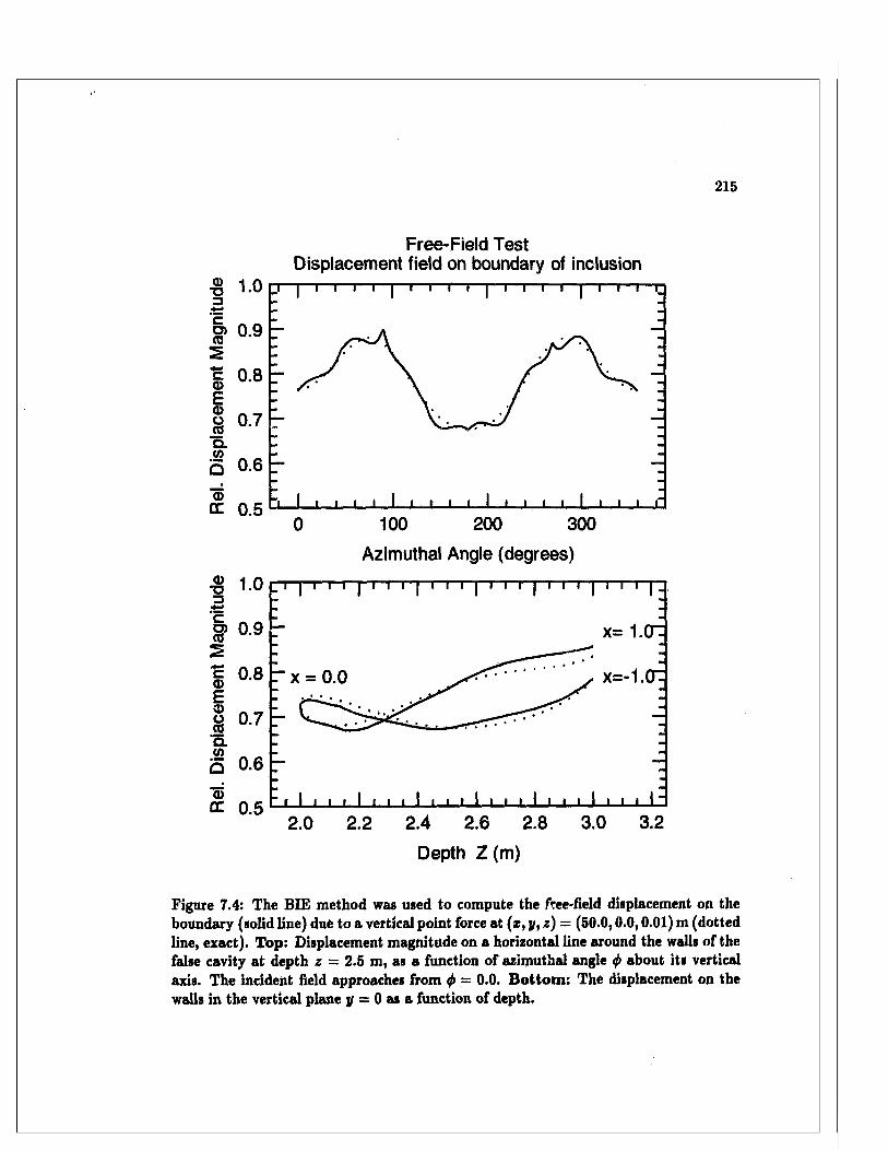
2151.
Dis
plac
emen
t M
agni
tude
o o
o o
-*•
b> ‘■>j
a>
co o
Free-Field Test Displacement field on boundary of inclusion
t y r i—■ —r..y t j— 1 1 —| -i 1 1 r | r—r ~i i_
©EC 0.5 "1 1 1 1 1 1 1 1 1 1 1 1 • 1 1 1 1 1 1 1 f
0 100 200 300
-g 1.0
o) 0.9 co2c 0.8ECDS3 0.7CO
I 0.6
Azimuthal Angle (degrees)
_ 1 | 1 1 r | t r 1 | 1 1 *1 | 1 1 1 | 1 r 1 | r 1 1 | _
r x= l.or
r x=-1 .or:
m 1“
"3)CC 0 . 5
" 1 1 1 1 1 1 1 1 1 1 1 1 1 1 1 1 1 1 1 1 1 1 1 1 1 12.0 2.2 2.4 2.6 2.8 3.0 3.2
Depth Z ( m)
Figure 7.4: The BIE method was used to compute the free-field displacement on the boundary (solid line) due to a vertical point force at (z, y, z) = (50.0,0.0,0.01) m (dotted line, exact). Top: Displacement magnitude on a horizontal line around the walls of the false cavity at depth z = 2.5 m, as a function of azimuthal angle <j> about its vertical axis. The incident field approaches from <j> = 0.0. B ottom : The displacement oil the walls in the vertical plane y = 0 as a function of depth.
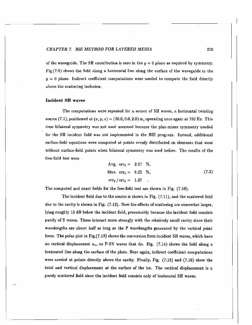
C H A P T E R 7. B IE M E TH O D F O R L A Y E R E D M ED IA 216
of the waveguide. T he SH contribution is zero in the y = 0 plane as required by symmetry.
Fig.(7.9) shows the field along a horizontal line along the surface of the waveguide in the
y = 0 plane. Indirect coefficient com putations were needed to com pute the field directly
above the scattering inclusion.
Incident SH waves
The com putations were repeated for a source of SH waves, a horizontal tw isting
source (7.1), positioned a t (x, y, z) — (50.0,0.0,2.0) m, operating once again a t 750 Hz. This
time bilateral sym m etry was not used assumed because the plus-minus sym m etry needed
for the SH incident field was not implemented in the BIE program . Instead, additional
surface-held equations were com puted at points evenly d istributed on elements th a t went
w ithout surface-held points when bilateral sym m etry was used before. T he results of the
free-held test wereAvg. erri = 2.17 %,
Max. erri = 8.25 %, (7.3)
err2 / erri = 1 . 3 7
The com puted and exact helds for the free-held test are shown in Fig. (7.10).
T he incident held due to the source is shown in Fig. (7.11), and th e scattered held
due to the cavity is shown in Fig. (7.12). Now the effects of scattering are somewhat larger,
lying roughly 13 dB below the incident held, presumably because the incident held consists
purely of S waves. These in teract more strongly with the relatively small cavity since their
wavelengths are abou t half as long as the P wavelengths generated by the vertical point
force. The polar plot in Fig.(7.13) shows the conversion from incident SH waves, which have
no vertical displacement uz , to P-SV waves th a t do. Fig. (7.14) shows the held along a
horizontal line along the surface of the plate. Here again, indirect coefficient com putations
were needed at points directly above the cavity. Finally, Fig. (7.15) and (7.16) show the
total and vertical displacement a t the surface of the ice. The vertical displacement is a
purely scattered held since the incident held consists only of horizontal SH waves.
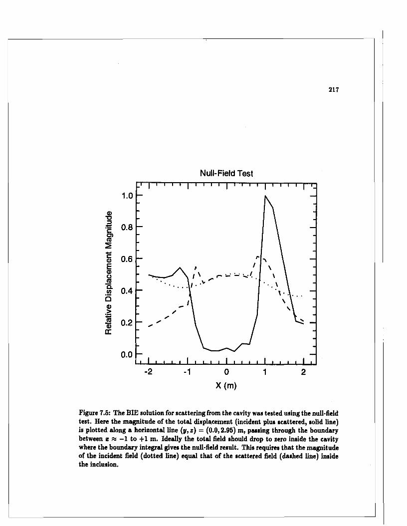
217
Null-Field Test
a>■a
" 0.8S’2
1 0.6 -
E
sw 0.4 -
50)>
0.2 -5a>0C
0.0
2 1 0 1 2X (m)
Figure 7.5: The BIE solution for scattering from the cavity was tested using the null-held test. Here the magnitude of the total displacement (incident plus scattered, solid line) is plotted along a horizontal line (y, z) = (0.0,2.95) m, passing through the boundary between z « —1 to +1 m. Ideally the total field should drop to zero inside the cavity where the boundary integral gives the null-field result. This requires that the magnitude of the incident field (dotted line) equal that of the scattered field (dashed line) inside the inclusion.
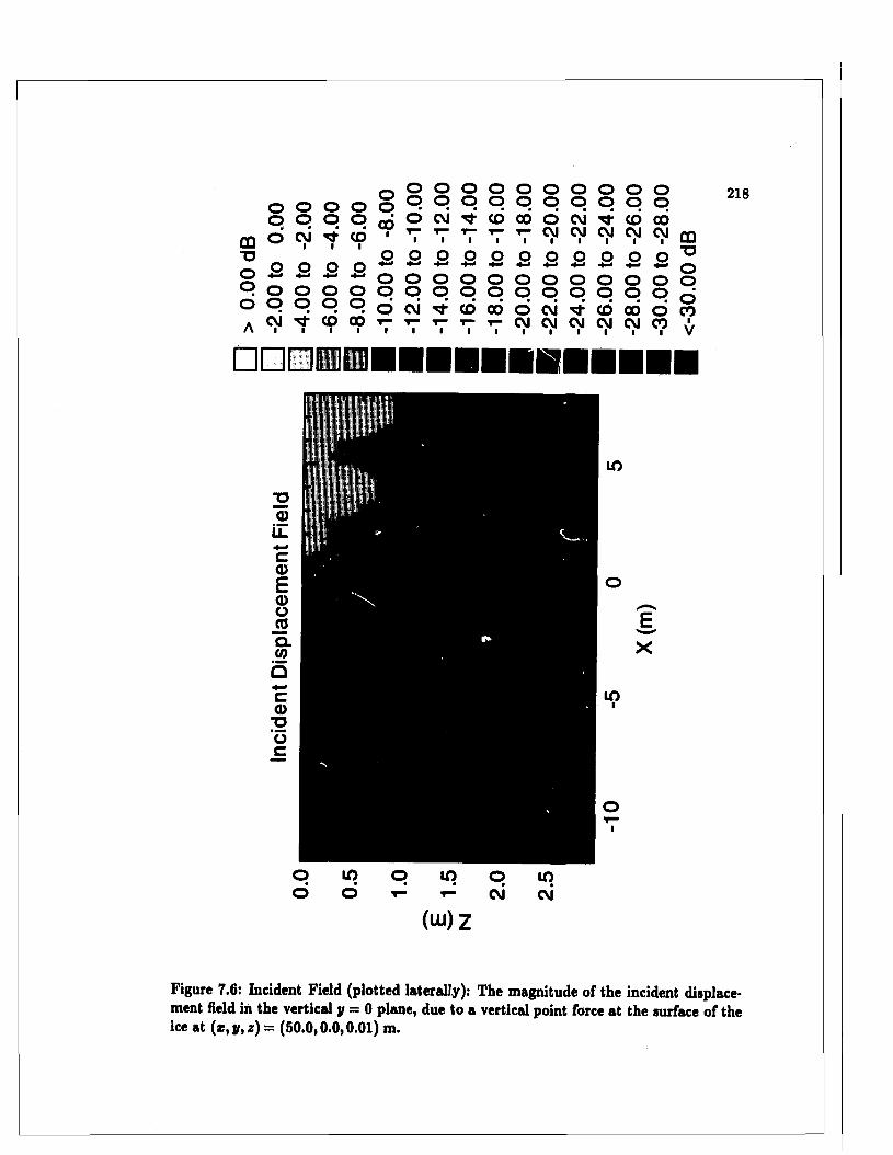
CDT3OOO
OOo
oocvjI
ooc\iI
oo
I
o0 o o 9 P 00<<t CD 'I I op o ■*-*
oo o o 9 9 oC O 0 0 T -
1 I I
o o o o o o o op p p p p p p o © c \ i - ' f r c d c o d c \ i T i :T - T - T - T - l - C V J C V J C V J■ ■ i i i ■ i io o o o o o o o o oO O O O O O O O O Op p p p p p p p p oc v i ^ t c d o d d o i ' ^ - c o o o dY , : T7 , " w w c y i c \ i c \ i w• • i i i i i i i i
o o o oCO 00^ ^ CD o o
0 oo001V
2 1 8
□□□I u m m u u m s m u m u m
in
20)
L i.c0Eoo0Q.0 X
c0
“Ooc
inI
o in o in o m• • • • • i
O O i - t - CM CM
(uj) z
Figure 7.6: Incident Field (plotted laterally): The magnitude of the incident displacement field in the vertical y = 0 plane, due to a vertical point force at the surface of the ice at (*, y, z) = (50.0,0.0,0.01) m.
219O CO O CO
o oo ooCMIA
s o c o N o n s o c o p p c o p p p p o p c v i ^ i r j c d c o d d c N i c oC V I C MC V I C MC V I C MC O C O C O
0 0 0 0 0 0 0 0 0 0 0 0 0 04-4 4-4 4-4 +- 4-» 4-< 4^ 4—> 44 44 4-4 4-4 4-4O S O O N O C O N O C O N O C O Nc o c q p c o p p c o c q p o o p p e q c q r ^ w ^ i n c D c d o i d a i c o ^ c D N c d C M C M C M C M C M C M C M O O O O O O C O C O O O O O
N O O N P O 00 p
CD N CO CO CO CO CO c q
O *o
o oP oo -t t V
□□□I
o in o m o tno o T-’ t-’ cvi cvi
(W)ZFigure 7.7: Scattered Field (plotted laterally): The magnitude of the scattered displacement field in the vertical y = 0 plane. The dark band is the zone in which indirect coefficient computations are required, but were omitted to reduce the computation time. The incident field is that of a vertical point force at the surface of the ice at (ss, y, z) = (50.0,0.0,0.01) m.
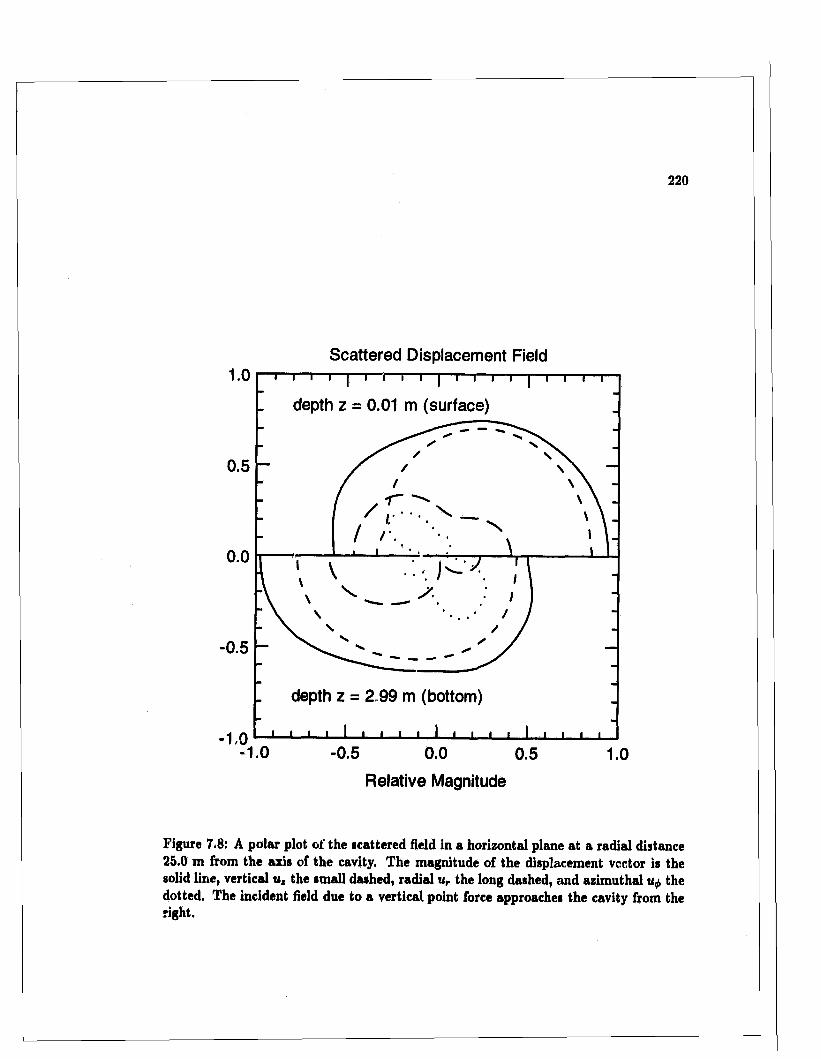
220
Scattered Displacement Field1.0
depth z = 0.01 m (surface)
0.5
0.0
-0.5
depth z = 2.99 m (bottom)
1 . 0 '— - 1.0 -0.5 0.0 0.5 1.0
Relative Magnitude
Figure 7.8: A polar plot of the scattered field in a horizontal plane at a radial distance25.0 m from the axis of the cavity. The magnitude of the displacement vector is the solid line, vertical u* the small dashed, radial ur the long dashed, and azimuthal tty the dotted. The incident field due to a vertical point force approaches the cavity from the right.

221
Scattering from a hemispherical cavity Displacement along the ice surface, z = 0.01 m
<D■o
1 0.8ca
2
1 0.6£<D
joS' 0.4 a<D>
2 0.2 ©DC
0.0
2 01 0-10 0-20X(m)
Figure 7.9: The displacement field along a horizontal line (y, z) ~ (0,0.01) passing over th< cattering cavity. The total field is the solid line, the incident the dotted, and the scattered the dashed. Indirect coefficient computations were used at points directly above the cavity, between as = - 1 to +1.
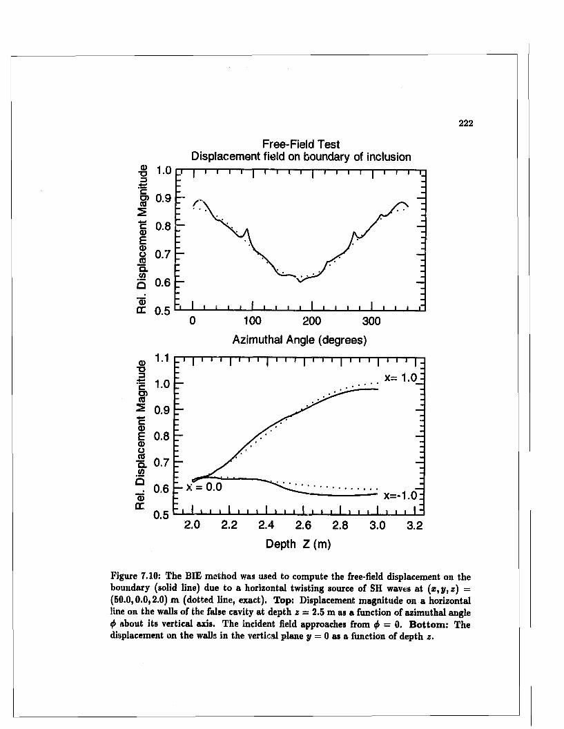
222
Free-Field Test Displacement field on boundary of inclusion
a>TJ=3'c
20.9
c 0.8 (UE
& 0.7coQ.V)5 0.6a>DC 0.5
0 1 0 0 200 300Azimuthal Angle (degrees)
<D~o=J x=
' c5?
2 0.9a>E 0.8<DS ft -7o 0.7 w
E! 0,6a>DC
0.5
0.0
2.0 2.2 2.4 2.6 2.8 3.0 3.2Depth Z (m)
Figure 7.10: The BIE method was used to compute the free-held displacement on the boundary (solid line) due to a horizontal twisting source of SH waves at (x, y, z) = (50.0,0.0,2.0) m (dotted line, exact). Top: Displacement magnitude on a horizontal line on the walls of the false cavity at depth z = 2.5 m as a function of azimuthal angle <f> about its vertical axis. The incident field approaches from <f> = 0. B ottom : The displacement on the walls in the vertical plane y — 0 as a function of depth z.

e § S3S OQ3 gHthA
A
W 3* A ® a D.- ° 2 8* o a g. ■ «■- ° o ' *TJr° e . s '
S « e £II3 *c <=> t v Sf £ 2 § S -® S*p*-CL A e- *i§ I s
o i
cr erA
S g 5-1£. B.3- c ^ o. S' *-• s,*2 ? “ Ao _5 g S I :- IU5 - « §=« s . 5 ®< n A A
N
Incident D isplacem ent Field
X (m)
> 0.00 dB -2.00 to 0.00 -4.00 to -2.00 -6.00 to -4.00 -8.00 to -6.00 -10.00 to -8.00 -12.00 t o -10.00 -14.00 t o -12.00 -16.00 t o -14.00 -18.00 t o -16.00 -20.00 t o -18.00 -22.00 to -20.00 -24.00 to -22.00 -26.00 to 24.00 -28.00 to -26.00 -30.00 to -28.00 <-30.00 dB
tot oCO
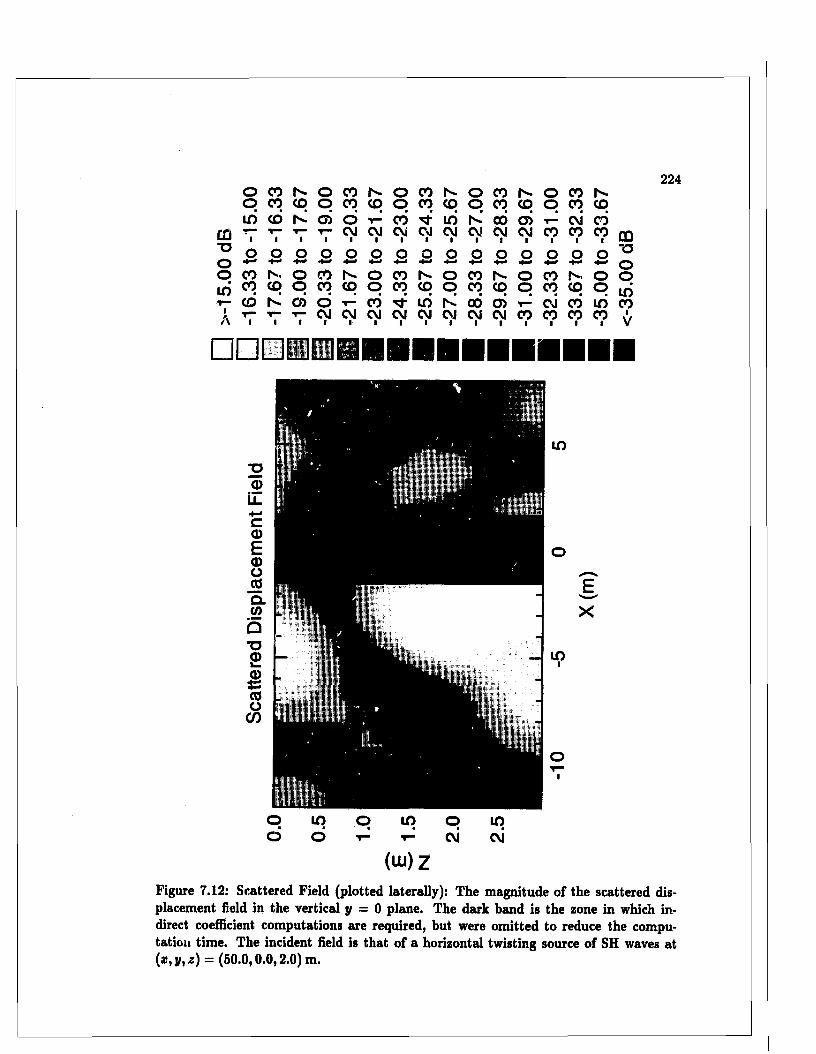
224
CO~oOOLO■Y—IA
oo
COCO
h -CO
oo CO
COIS.p
oo COCO
NCO
oo COCO
h*CO
oo
COCO
Is .CO
in’ I
CO1
fs!
1CD
1oCVII
■V—CVI1
COCVI1 CVI1
inCVI1
N-'CV!1
00CVI1
CDCVI1 CO1
cviCOI
COCO1
o■*—> o o o o o o■4—> o o o o*-* o•*-* o o o
COCO
h»CO
oo COCO
IS.p
oo COCO
r".CO
oo COCO
IS.p oo COCO
f sCO
ooCOT"—
1NT—
1CD
1oCVI1 cvi1
COCVI1 CVI1
inCVI1
|s!CVI1
0 0CVI1
dCVI1 CO1
cviCOI
COCO1
inCO1
~oOOincoV
□ □ □
E.x
(u j ) zFigure 7.12: Scattered Field (plotted laterally): The magnitude of the scattered displacement field in the vertical y = 0 plane. The dark band is the zone in which indirect coefficient computations are required, but were omitted to reduce the computation time. The incident field is that of a horizontal twisting source of SH waves at (x ,y ,z) = (50.0,0.0,2.0) m.
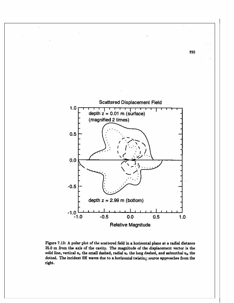
Scattered Displacement Field
depth z = 0.01 m (surface) (magnified 2 times)
0.5
0.0
-0.5
depth z = 2.99 m (bottom)
- 1.0- 1.0 -0.5 0 .0 0.5 1.0
Relative Magnitude
Figure 7.13: A polar plot of the scattered field in a horizontal plane at a radial distance25.0 m from the axis of the cavity. The magnitude of the displacement vector is the solid line, vertical uz the small dashed, radial ur the long dashed, and azimuthal u<* the dotted. The incident SH waves due to a horizontal twisting uource approaches from the right.
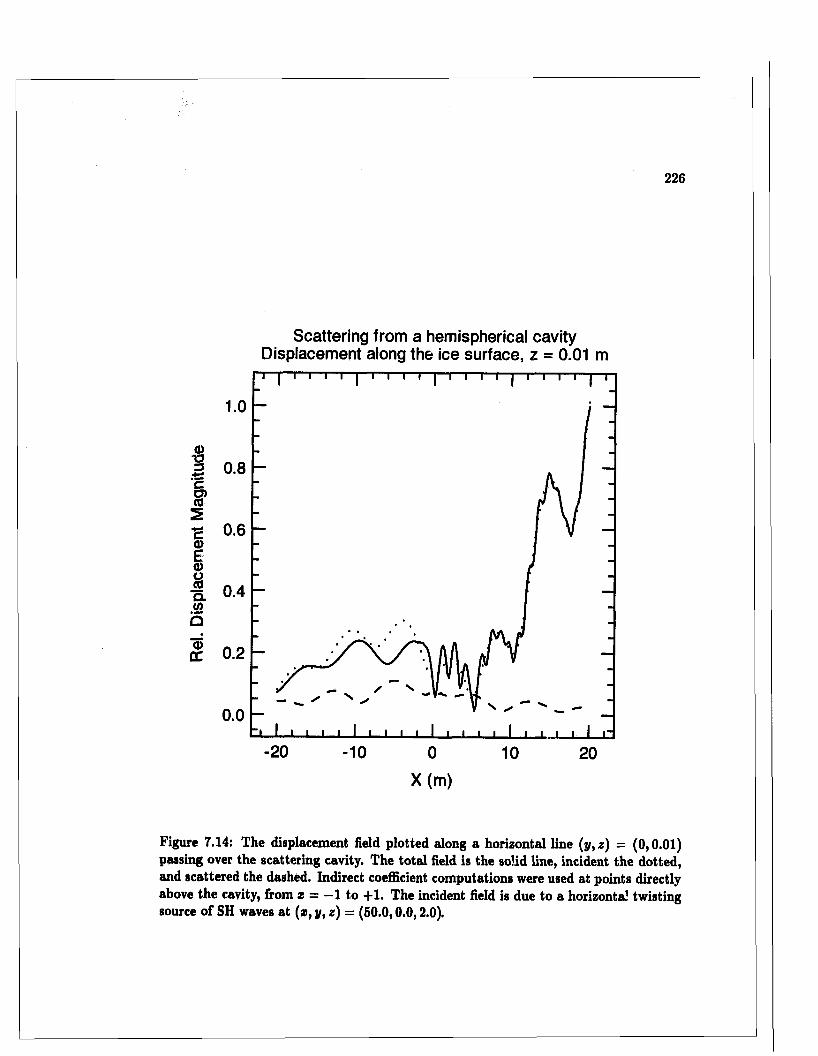
226
Scattering from a hemispherical cavity Displacement along the ice surface, z = 0.01 m
1.0
■ I ■ i ■ i I i i i i | r i i i | r i i i | i
Rel
. D
ispl
acem
ent
Mag
nitu
de
o O
O O
ro
Ip* b>
00
! f \
0.0~i i i i i i i i i i i i i i i i i i i i i i i-
-20 -10 0 10 20
X(m)
Figure 7.14: The displacement field plotted along a horizontal line (y, z) = (0,0.01) passing over the scattering cavity. The total field is the solid line, incident the dotted, and scattered the dashed. Indirect coefficient computations were used at points directly above the cavity, from x = —1 to +1. The incident field is due to a horizontal twisting source of SH waves at (*, y, z) = (50.0,0.0,2.0).
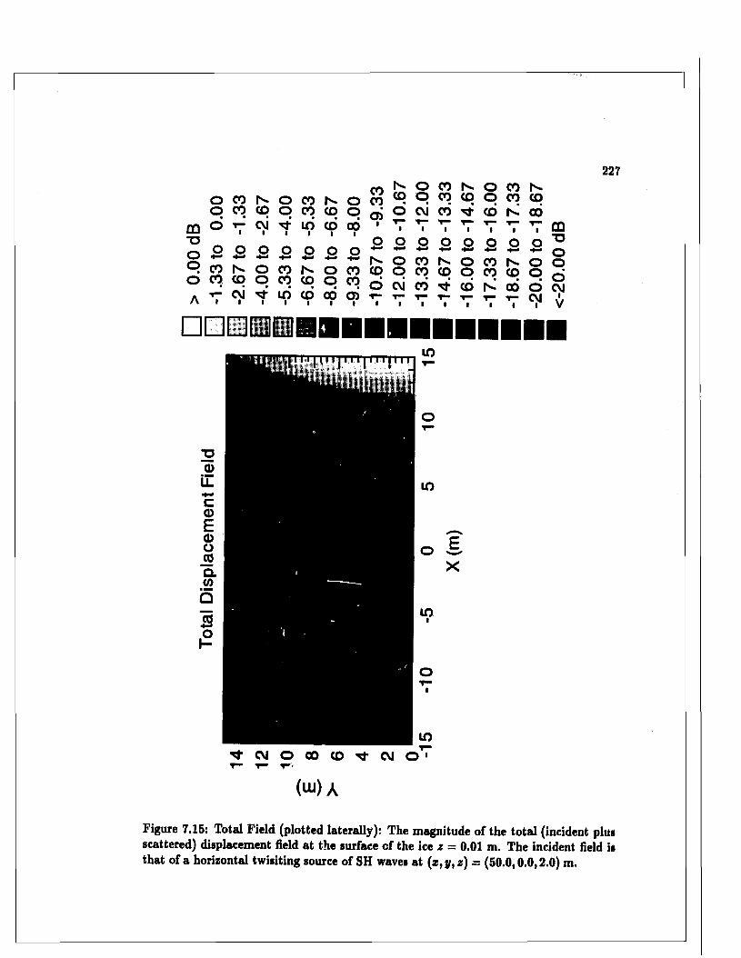
227
OO
00CO
h*CO
oo
COCO
1CO
oo
CD o 1 cvi12
1 to CD COT3O o o
*—• o o o1
sOo
00CO
h-CD
oo
00CO
1CO
oo
CO00
A 1 cvia 1 l61 CO1 001 d1
COCOCT>i
O
h -
o CO 1 o CO f"-CO o CO p o CO COo cvi CO "'d- CD 00T -1 1 1 1 1 1 1 CDo o o o o o o T34 ^ *—■ +-* oo 0 0 h . o 0 0 o oo CO CO o CO CO o ocvi CO - 'f r CD 1 00 o CVI1 T —1 T—1 1—1 1-1 1 CVI1
1V
[ H E H [ H i l l
m 1 1 1 1 jT T i 111111111111 ■'i' | |
E
X
^ C M O C O C O ^ t C V I O
(u i)A
Figure 7.15: Total Field (plotted laterally): The magnitude of the total (incident plus scattered) displacement field at the surface of the ice z = 0.01 m. The incident field is that of a horizontal twisiting source of SH waves at (x , y , z ) = (50.0,0.0,2.0) m.
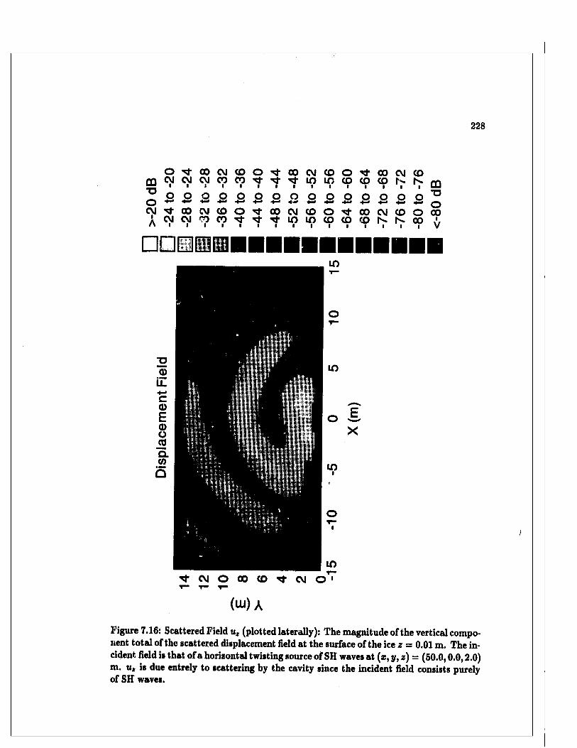
TJOCMIA
O Tf 00 CM CD O
^ 00 CM 0 O ^ CM CM CO CO ^ M-i i i i i i
228
□ □ □
00 CM CO o 00 CM CO1 "M-i in• ini CO1 CO1 CO1 r-■ N.■ CDo O o o o 2 o o o "D
■«-* *—• •*-> o00 CM CO o 00 CM CO o 001 in■ in■ CO1 CO1 CO1 r-1 h-1 001
■V
]D<Di l■*->c<DE<DOCOCLCO
I
in
E
X
ini
inCM O 00 CD Tf CM o V
(Ui) A
Figure 7.16: Scattered Field u4 (plotted laterally): The magnitude of the vertical component total of the scattered displacement field at the surface of the ice z = 0.01 m. The incident field is that of a horizontal twisting source of SH waves at ( x , y , z ) = (50.0,0.0,2.0) m. u, is due entrely to scattering by the cavity since the incident field consists purely of SH waves.
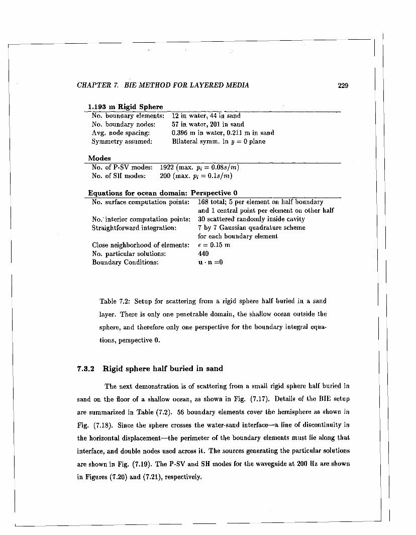
C H A P T E R 7. B IE M E TH O D F O R L A Y E R E D M ED IA
1.193 m Rigid Sphere
229
No. boundary elements: No. boundary nodes: Avg. node spacing: Symmetry assumed:
Modes
12 in w ater, 44 in sand 57 in w ater, 201 in sand 0.396 in in water, 0.211 m in sand Bilateral symm. in y = 0 plane
No. of P-SV modes: No. of SH modes:
1922 (max. pi = 0 .08s/ro) 200 (max. pi = 0.1 s /m )
Equations for ocean domain: Perspective 0No. surface com putation points:
No. interior com putation points: S traightforward integration:
Close neighborhood of elements: No. particular solutions: Boundary Conditions:
168 total; 5 per element on half boundaryand 1 central point per element on other half30 scattered randomly inside cavity7 by 7 Gaussian quadrature schemefor each boundary elemente = 0.15 m440u n =0
Table 7.2: Setup for scattering from a rigid sphere half buried in a sand
layer. There is only one penetrable domain, the shallow ocean outside the
sphere, and therefore only one perspective for the boundary integral equa
tions, perspective 0.
7.3.2 Rigid sphere half buried in sand
T he next dem onstration is of scattering from a small rigid sphere half buried in
sand on th e floor of a shallow ocean, as shown in Fig. (7.17). Details of the BIE setup
are summarized in Table (7.2). 56 boundary elements cover the hemisphere as shown in
Fig. (7.18). Since the sphere crosses th e water-sand interface—a line of discontinuity in
the horizontal displacement— the perim eter of the boundary elements m ust lie along tha t
interface, and double nodes used across it. The sources generating the particular solutions
are shown in Fig. (7.19). The P-SV and SH modes for the waveguide a t 200 Hz are shown
in Figures (7.20) and (7.21), respectively.
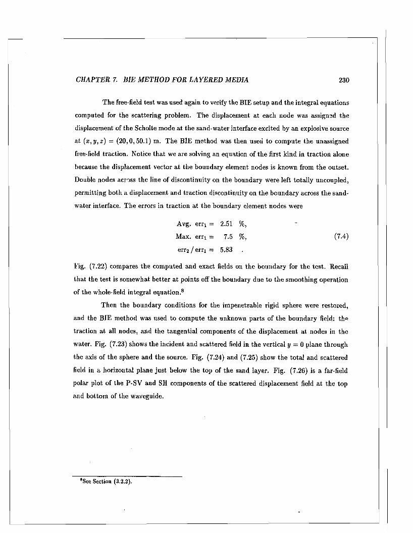
C H A P TE R 7. B IE M ETH O D F O R L A Y E R E D M ED IA 230
The free-field test was used again to verify the BIE setup and the integral equations
computed for the scattering problem . The displacement a t each node was assigned the
displacement of the Scholte m ode at the sand-water interface excited by an explosive source
at (x , y , z ) = (20 ,0 ,50.1) m. T he BIE m ethod was then used to com pute the unassigned
free-field traction. Notice th a t we are solving an equation of th e first kind in traction alone
because the displacement vector a t the boundary element nodes is known from the outset.
Double nodes across the line of discontinuity on the boundary were left totally uncoupled,
perm itting both a displacement and traction discontinuity on the boundary across the sand-
water interface. The errors in traction at the boundary element nodes were
Avg. e rri = 2.51 %,
Max. e rri = 7.5 %, (7.4)
err2 / erri = 5.83
Fig. (7.22) compares the com puted and exact fields on the boundary for the test. Recall
tha t the test is somewhat be tte r a t points off the boundary due to the sm oothing operation
of the wlvole-field integral equation.8
T hen the boundary conditions for the im penetrable rigid sphere were restored,
and the BIE m ethod was used to com pute the unknown parts of the boundary field: the
traction a t all nodes, and the tangential components of the displacement at nodes in the
water. Fig. (7.23) shows the incident and scattered field in the vertical y = 0 plane through
the axis of the sphere and the source. Fig. (7.24) and (7.25) show the to ta l and scattered
field in a horizontal plane ju st below the top of the sand layer. Fig. (7.26) is a far-field
polar plot of the P-SV and SH com ponents of the scattered displacement field a t the top
and bottom of the waveguide.
*See Section (3.2.2).
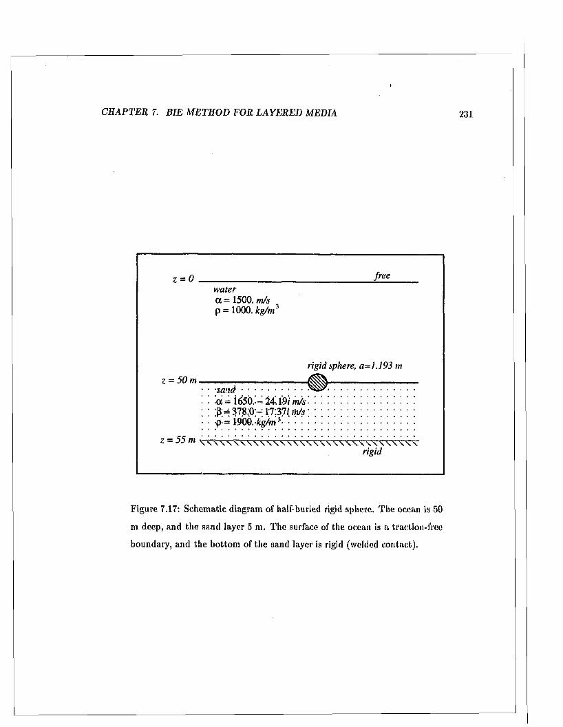
C H A P TE R 7. B IE M E TH O D F O R L A Y E R E D M ED IA 231
freez = 0
watera = 1500. m/s p = 1000. kg/m
rigid sphere, a= I.J93 m
z = 50 msanda = 1650..-> 241-9/ m/s
p.= 1900. kg/m
z = 55 m ^ \ \ \rigid
Figure 7.17: Schem atic diagram of half-buried rigid sphere. T he ocean is 50
m deep, and the sand layer 5 m. The surface of the ocean is a traction-free
boundary, and the bo ttom of the sand layer is rigid (welded contact).
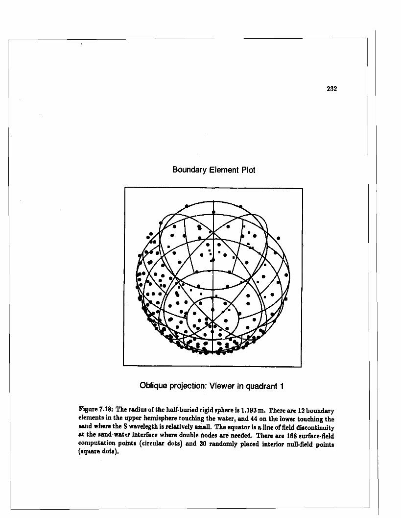
232
Boundary Element Plot
• • •
Oblique projection: Viewer in quadrant 1
Figure 7.18: The radius of the half-buried rigid sphere is 1.193 m. There are 12 boundary elements in the upper hemisphere touching the water, and 44 on the lower touching the sand where the S wavelegth is relatively small. The equator is a line of field discontinuity at the sand-wat er interface where double nodes are needed. There are 168 surface-field computation points (circular dots) and 30 randomly placed interior null-held points (square dots).
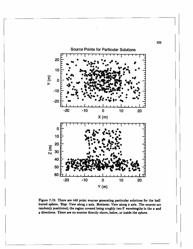
233
Source Points for Particular Solutions
20
1 0
I 0 >-
- 1 0
- 2 0
0
1 0
_ 2 0 E
N 3 0
40
50
60
Figure 7.19: There are 440 point sources generating particular solutions for the half- buried sphere. Top: View along z axis. B ottom : View along x axis. The sources are randomly positioned; the region covered being roughly two P wavelengths in the x and y directions. There are no sources directly above, below, or inside the sphere.
| I i I I | i I I l | I l l l | l l l I | I.
- . . • £ • * * . . * * • *
* ; > ; V .
• * . * v v f * • « • • *■ m • • • V • • Hl—1 i_ . I I J - I A I I _t I I I I I I I I I . I -20 -10 0 10 20
X (m)
HR
H < m
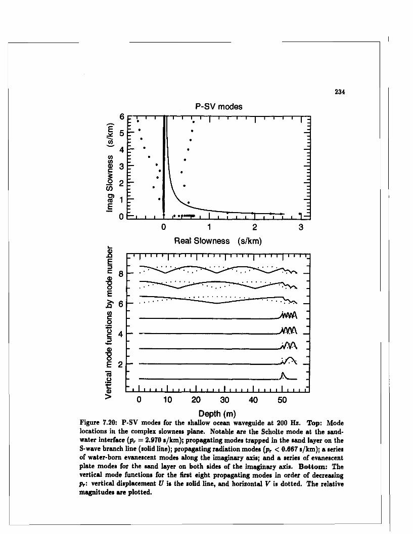
234
P-SV modes6
5
4
3
2
00 1 32
Real Slowness (s/km)
8
£ 6
4
2
o>> 0 1 0 2 0 30
Depth (m)Figure 7.20: P-SV inodes for the shallow ocean waveguide at 200 Hz. Top: Mode locations in the complex slowness plane. Notable are the Scholte mode at the sand- water interface (pr — 2.970 s/km); propagating modes trapped in the sand layer on the S-wave branch line (solid line); propagating radiation modes (pr < 0.667 s/km); a series of water-born evanescent modes along the imaginary axis; and a series of evanescent plate modes for the sand layer on both sides of the imaginary axis. B ottom : The vertical mode functions for the first eight propagating modes in order of decreasing pr: vertical displacement U is the solid line, and horizontal V is dotted. The relative magnitudes are plotted.
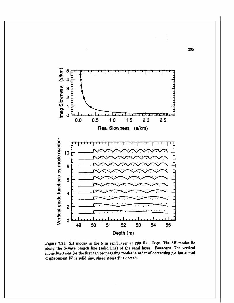
236
S2, 4
Q)j_=ti
2.52 .00 .0 0.5 1 .0 1.5
Real Slowness (s/km)
E r nE ;= 1 0 -0)E :E 8 -
-QViI 6 r
a>EECOota)
>
Depth (m)
Figure 7.21: SH modes in the 5 m sand layer at 200 Hz. Top: The SH modes lie along the S-wave branch line (solid line) of the sand layer. B ottom : The vertical mode functions for the first ten propagating modeB in order of decreasing pri horizontal displacement W is solid line, shear stress T is dotted.

Free-Field Test
■o3♦jCO)CO
2
0.8z = 50.01 m
0 .6co
0.4 z = 50.25
• 0 .2 z = 49.750)tro .o
o 1 0 0 2 0 0 300
Azimuthal Angle (degrees)
CD
p 0.8•*—*ccnco
5 0 .6co
0.4
oS 0.2 GC
0 .00 50 1 0 0 150
Vertical Angle (degrees)
Figure 7.22: Free-Field Test: The BIE method was used to compute the free-field traction (solid line) at the boundary due to an incident Scholte mode (dotted line, exact). Top: Traction magnitude on three horizontal lines around the walls of the false sphere as a function of azimuthal angle (j>. The incident Scholte mode approaches from ? = 0.0. B ottom : Traction in the vertical y = 0 plane as a function vertical angle 0 from the center for the sphere; 6 = 0 points vertically downwards. The sand-water interface is evident from the discontinuity at 90 degrees due to the edge at the ice-water interface, z = 3.0 m.
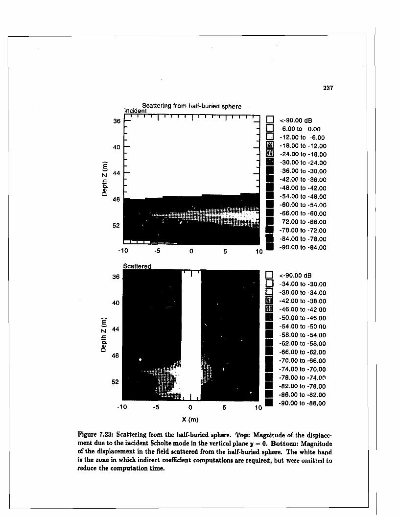
237
36
40
E*N 44ao>a
t . t Scattering from half-buried sphere IncidentT------
48
52
T I I
-10
T“|—r" i T i—i i i T t i " I i
_' &
10
□ <-90.00 dB□ -6.00 to 0.00□ -12.00 to -6.00Eg -18.00 to -12.00B -24.00 to -18.00■ -30.00 to -24.00■ -36,00 to -30.00■ -42.00 to -36.00■ -48.00 to -42.00■ -54.00 to -48.00■ -60.00 to -54.00■ -66.00 to -60.00■ -72.00 to -66.00■ -78.00 to -72.00■ -84.00 to -78.00■ -90.00 to -84.00
Scattered
^ i,:! PH;!1
□ <-90.00 dB□ -34.00 to -30.00El -38.00 to -34.00B -42.00 to -38.00■ -46.00 to -42.00■ -50.00 to -46.00■ -54.00 to -50.00■ -58.00 to -54.00■ -62.00 to -58.00■ -66.00 to -62.00■ -70.00 to -66.00■ -74.00 to -70.00■ -78.00 to -74.00■ -82.00 to -78.00■ -86.00 to -82.00■ -90.00 to -86.00
Figure 7.23: Scattering from the half-buried sphere. Top: Magnitude of the displacement due to the incident Scholte mode in the vertical plane y = 0. B ottom : Magnitude of the displacement in the field scattered from the half-buried sphere. The white band is the zone in which indirect coefficient computations are required, but were omitted to reduce the computation time.
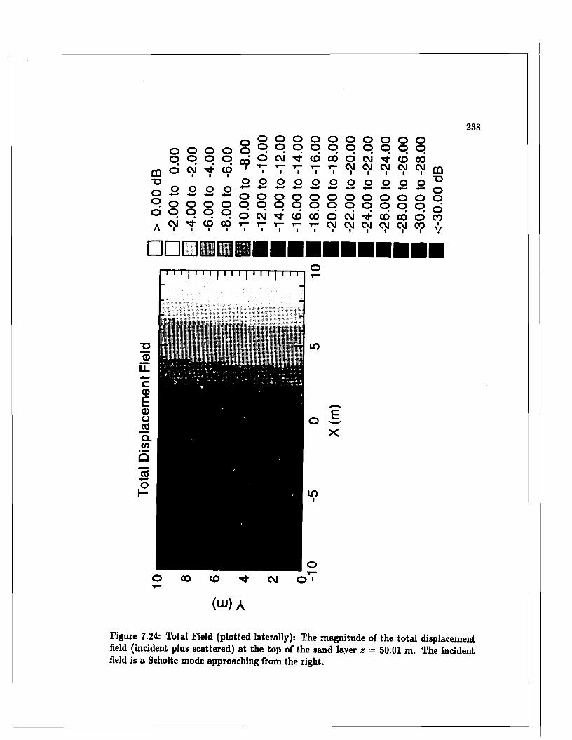
238, - * 0 0 0 0 0 0 0 0 0 0
CD -oOo oA
□
T 'T 'T ] I I I | I I I | I I I | I I I I y l
O 00 CO CVJ O '
(w) A
Figure 7.24: Total Field (plotted laterally): The magnitude of the total displacement field (incident plus scattered) at the top of the sand layer z = 50.01 m. The incident field is a Scholte mode approaching from the right.
OOO
OocviI
oo
■
ooCDI
oGOi
q q q q q o q q q q d a i ^ - c D o o d c M ^ t c o o d
. 2 . 2 0 0 0 0 0 0 0 0 +■* ■*— ■*-* •*—> 4 - ■«-. ■*-* 4S
oocvi■
oo
■
oo
oo
CO 00I I
ooo
oocvi
oo
CVJ CVJ CVI CVI c v i r n I I I I I u j
O O O O O " 0 O
O O O O O . o o o o q
c D G o d c v i ^ c o o o d c ot- t- C V J C V J C V J C V I C V I O O •■ ■ ■ ■ 1 1 1 1 /
oo
o o o o
oo
0 1
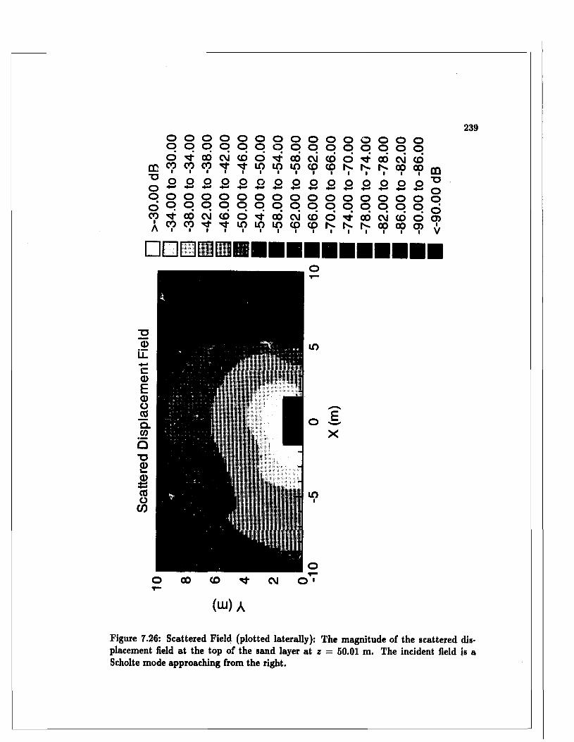
239
■oOOOCOIA
oo
oo
oo
oo
oo
oo
oo
oCOl CO1
GOCO1
cvi■
cd1
oin1 inI
o o+-> o o o+-> o o+->oo
oo
oo
oo
oo
oo
oo
CO0 0CO
cvi cd■st
om in
0 0in
O O Oo o o00 cvi CD L0 CO COI
o o o o o o o o o oIo
o o o o o ocvi cd oCD CO N
oo
oo
oo
oo
oo
o■
Tf-•
00N1
cvi001
cd00l
o•*-* B o o ooo
oo
oo
Oo
oo
'd-N
00h*
cvi00
cd00
oo>
CD■DOOOo>iV
O i
E
X
Figure 7.26: Scattered Field (plotted laterally): The magnitude of the scattered displacement field at the top of the sand layer at z = 50.01 m. The incident field is a Scholte mode approaching from the right.
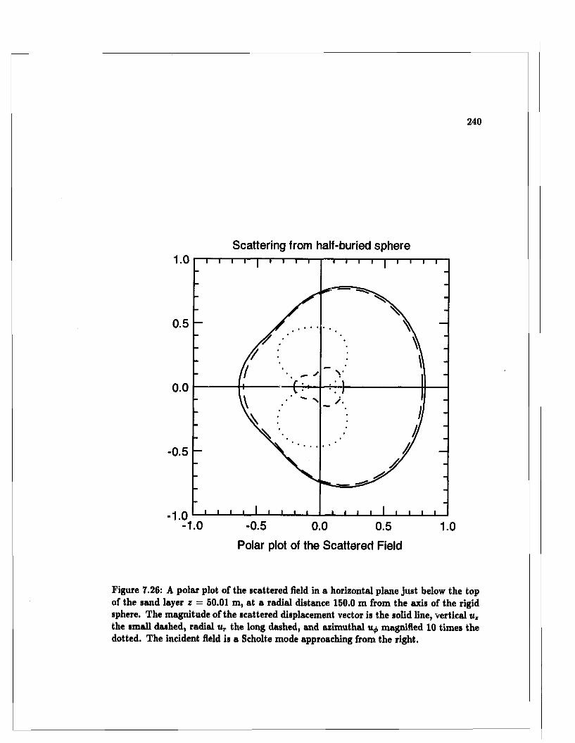
Scattering from half-buried sphere
0.5
0 . 0
-0.5
- 1 .0 -0.5 0 .0 0.5 1.0Polar plot of the Scattered Field
Figure 7.26: A polar plot of the scattered field in a horizontal plane just below the top of the sand layer z — 50.01 m, at a radial distance 150.0 m from the axis of the rigid sphere. The magnitude of the scattered displacement vector is the solid line, vertical uz the small dashed, radial ur the long dashed, and azimuthal magnified 10 times the dotted. The incident field is a Scholte mode approaching from the right.

C H A P T E R 7. B IE M ETH O D FO R L A Y E R E D M ED IA 241
7 .3 .3 C i r c u l a r ic e d o m e
The final dem onstration is of scattering from a circular ice dome in a 3 in ice plate.
A schematic of the model is shown in Fig. (7.27). The ice dome extends 2 m spherically up
out of th e waveguide, and 4 m down below the ice, into the water, as detailed in Fig. (7.28).
The details for the BIE m ethod are summarized in Table (7.3). There are two penetrable
domains, hence, uvvo perspectives for the integral equations: the exterior waveguide (per
spective 0) and the interior of the ice dome (perspective 1). T he two perspectives share 15
boundary elements inside the ice layer and sea wa„er, and the field is coupled across those
elements using continuity conditions applied at the nodes. Perspective 1 needs 9 additional
im penetrable elements to close the upper part of its boundary outside the waveguide, where
traction free t = 0 boundary conditions apply; hence, the interior domain is a m ixture of
both penetrable and im penetrable boundary elements.
T he G reen’s function for perspective 0 is for the Arctic waveguide considered earlier
in Table (5.1). T he G reen’s function for perspective 1 is for an unbounded homogeneous
ice domain. The P-SV modes for the Arctic profile at 20 Hz have been reported earlier:
the propagating in Fig.(5.6) and evanescent in (6.2). The SH modes for the ice plate at 20
Hz are shown in Fig. (7.29). SII modes in the sediments and bottom of the ocean are not
needed because their vibrations do not enter the water. Each perspective has its own set of
null-field points in their respective interior domain, as shown in Fig. (7.30). Each also lias
its own set of particu lar solutions for the indirect B IE m ethod; those of perspective 0 lying
within the waveguide—though not inside or directly below the scattering inclusion*"-, as
shown in Fig. (7.31), and those for perspective 1 distributed uniformly around the inclusion
in every direction, as shown in Fig. (7.32).
T he free-field test was used to test the integral equations and BIE setup for
both perspectives. T he free-field was due to a vertical point force acting at (u:, y, z) =
(200,0,0.01) m for both perspectives. Two tests were made for each perspective. In the
first the free-field boundary displacement was assigned to the nodes using boundary condi
tion equations, and the BIE m ethod was used to com pute the unassigned traction vector
(equation of the first kind); in the second, traction was assigned and displacement was
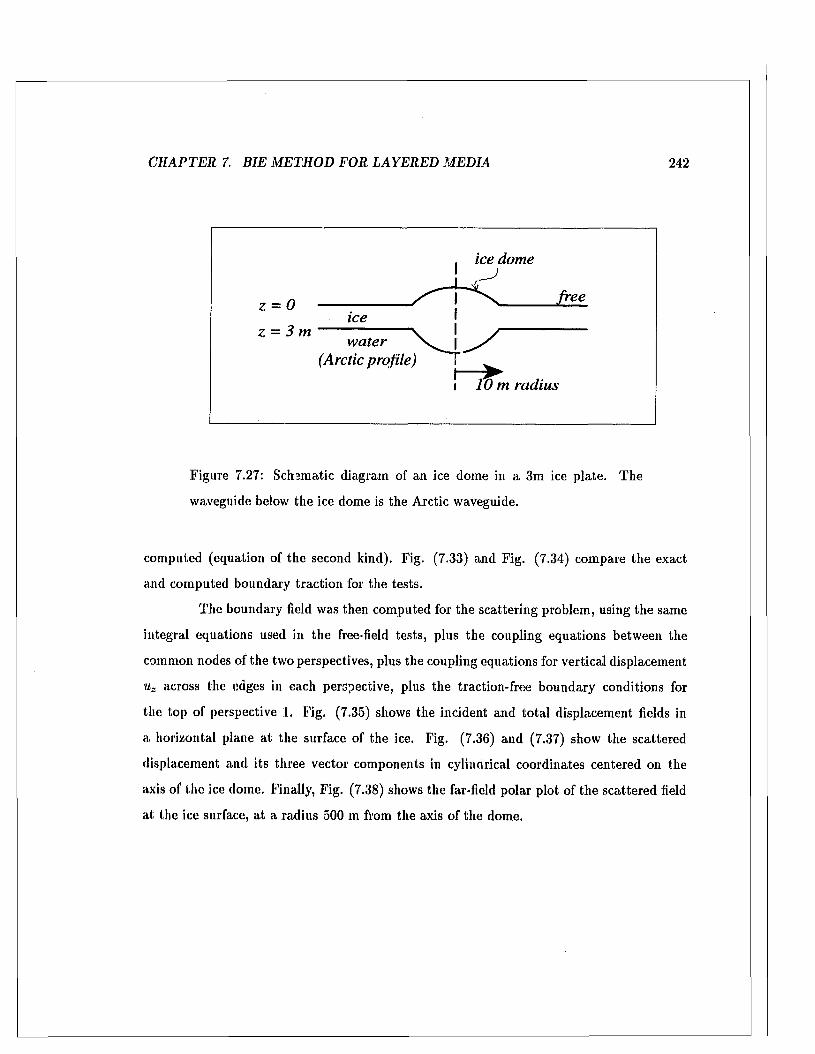
C H A P T E R 7. B IE M ETH O D FO R L A Y E R E D M E D IA 242
ice dome
fre ez = 0
z = 3 mice
w a ter \ I (Arctic profile) T
i 10 m radius
Figure 7.27: Schematic diagram of an ice dome in a 3m ice plate. The
waveguide below the ice dome is the Arctic waveguide.
com puted (equation of the second kind). Fig. (7.33) and Fig. (7.34) compare the exact
and com puted boundary traction for the tests.
The boundary field was then com puted for the scattering problem, using the same
integral equations used in the free-held tests, plus the coupling equations between the
common nodes of the two perspectives, plus the coupling equations for vertical displacement
uz across the edges in each perspective, plus the traction-free boundary conditions for
the top of perspective 1. Fig. (7.35) shows the incident and to ta l displacement helds in
a horizontal plane at the surface of the ice. Fig. (7.36) and (7.37) show the scattered
displacement and its three vector components in cylindrical coordinates centered on the
axis of the ice dome. Finally, Fig. (7.38) shows the far-held polar plot of the scattered held
at the ice surface, a t a radius 500 m from the axis of the dome.
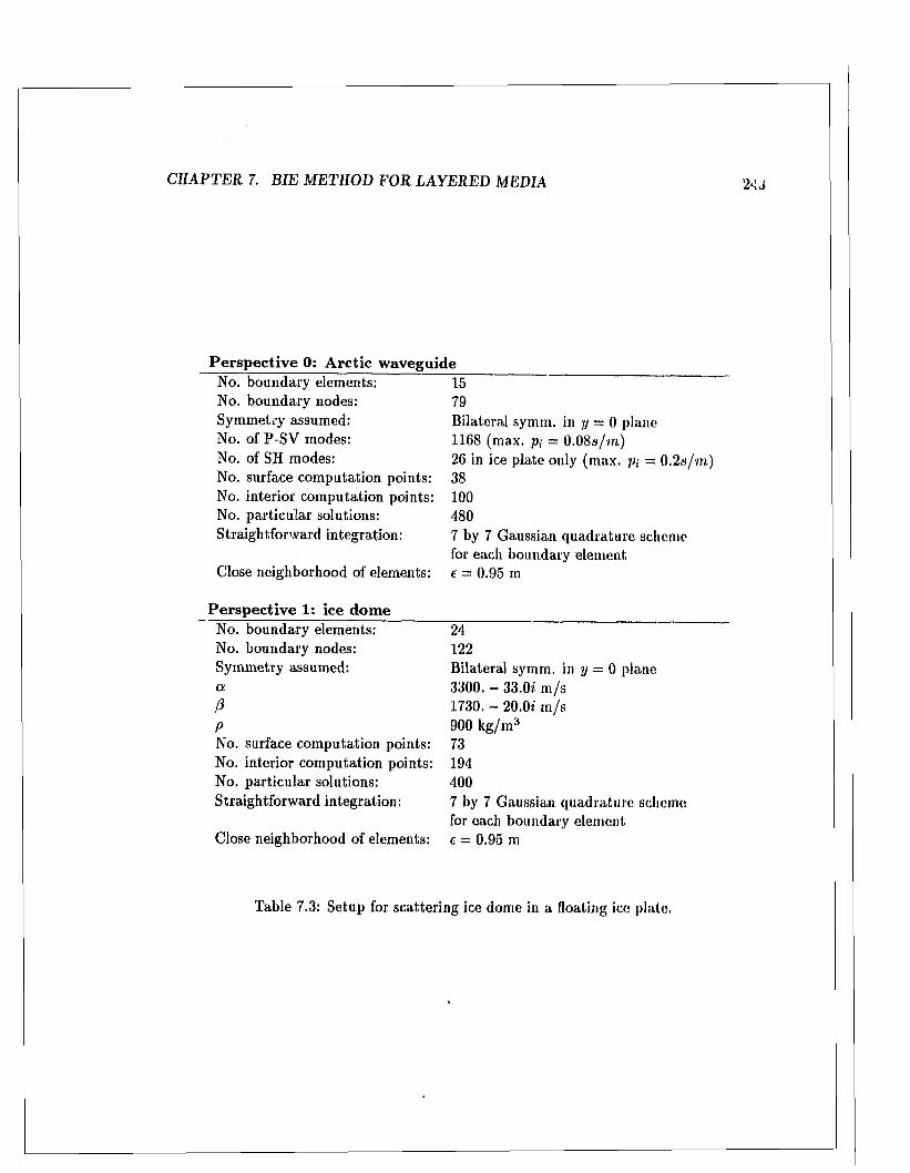
C H A P T E R 7. B IE M ETH O D F O R L A Y E R E D M EDIA
Perspective 0: Arctic waveguideNo. boundary elements:No. boundary nodes:Symmetry assumed:No. of P-SV modes:No. of SH modes:No. surface com putation points: No. interior com putation points: No. particu lar solutions: S traightforw ard integration:
Close neighborhood of elements:
1579Bilateral symm. in y = 0 plane 1168 (max. p; = O.OS-s/yn)26 in ice p late only (max. p,- = 0 .2s /m ) 38 100 4807 by 7 Gaussian quadrature scheme for each boundary element e = 0.95 m
Perspective 1: ice domeNo. boundary elements:No. boundary nodes:Symmetry assumed: aPPNo. surface com putation points: No. interior com putation points: No. particu lar solutions: Straightforw ard integration:
Close neighborhood of elements:
24122Bilateral symm. in y = 0 plane3300. - 33.0* m /s1730. - 20.0* m /s900 k g /m 3731944007 by 7 Gaussian quadrature scheme for each boundary element e = 0.95 m
Table 7.3: Setup for scattering ice dome in a floating ice plate.
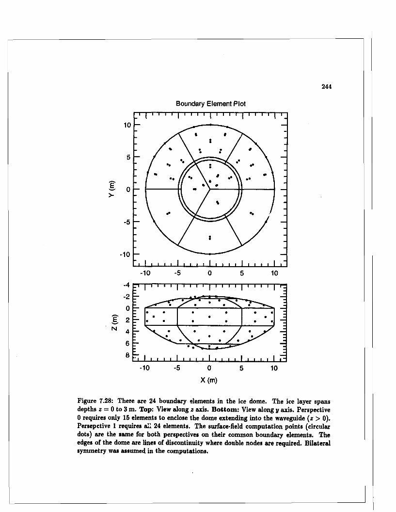
244
Boundary E lem ent P lot
•• ••E>
-10
-10 -5 0 5 10
4
2
0
2
4
6
8
-10 5 0 5 10
X (m)
Figure 7.28: There are 24 boundary elements in the ice dome. The ice layer spans depths z = 0 to 3 m. Top: View along z axis. B ottom : View along y axis. Perspective 0 requires only 15 elements to enclose the dome extending into the waveguide (z > 0). Persepctive 1 requires all 24 elements. The surface-field computation points (circular dots) are the same for both perspectives on their common boundary elements. The edges of the dome are lines of discontinuity where double nodes are required. Bilateral symmetry was assumed in the computations.
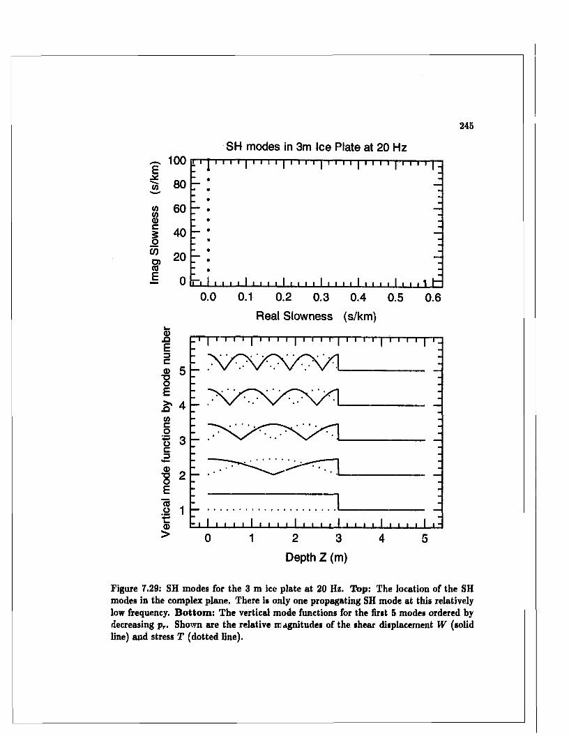
245
SH modes in 3m Ice Plate at 20 Hz100
Exe.1/3
WWCDcI05O)coE
i _ l I I I J _ l L I I I I 1 I I I I I I I I I I I I I I I I I 1 | ~
0.0 0.1 0.2 0.3 0.4 0.5 0.6
Real Slowness (s/km)
5
£ 4
3
2
1
<u> 10 2
Depth Z (m)
Figure 7.29: SH modes for the 3 m ice plate at 20 Hz. Top: The location of the SH modes in the complex plane. There is only one propagating SH mode at this relatively low frequency. B ottom : The vertical mode functions for the first 5 modes ordered by decreasing pr. Shown are the relative magnitudes of the shear displacement W (solid line) and stress T (dotted line).
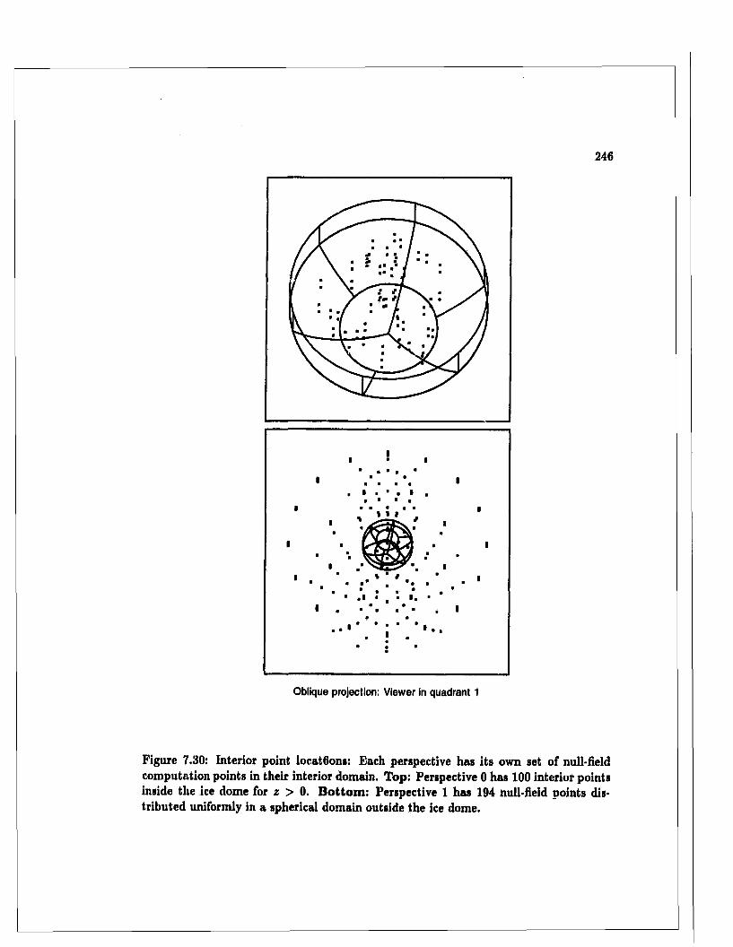
246
i* *i
i ■ t
■ .1 ■ . ■ i. •l . . i
• ■ ■............................a
• • ' , 1 ■ ■■ * m
Oblique projection: Viewer in quadrant 1
Figure 7.30: Interior point locat6ons: Each perspective has its own set of null-field computation points in their interior domain. Top: Perspective 0 has 100 interior points inside the ice dome for z > 0. B ottom : Perspective 1 has 194 null-held points distributed uniformly in a spherical domain outside the ice dome.
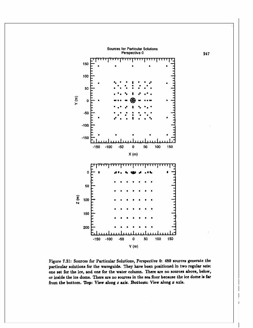
Sources for Particular Solutions Perspective 0 247
150_i p i t i p i r 111 i i 11 i t i t j n i'i | r T i r p “
— • • • • •
100
50
1 0 >
-50
-100
: . • • • • * • • • • . i
; ;
----- • W i t W ^ M • * M 1 —
I • • • • • * % • • • I
; • ;
-150• • • • • -
~i 1 i i i i 1 i i i i 1 i i i i 1 M i i 1 i i i i 1 i i i i i r-150 -100 -50 0 50 100 150
X(m)
j | t t n j 11 i i | n i t | n i r | i n i 1 1 1 1 1 1 1 ;
0 — • •<• • 1, « «i .SS. • —
50 _ —
•§ 100 N— ........................................... —
150
200~i 1 1 1 1 1 1 1 1 1 1 11 1 1 1 1 1 1 i i 1 1 1 1 1 1 1 1 1 i t r-150 -100 -50 0 50 100 150
Y(m)
Figure 7.31: Sources for Particular Solutions, Perspective 0: 480 sources generate the particular solutions for the waveguide. They have been positioned in two regular sets: one set for the ice, and one for the water column. There are no sources above, below, or inside the ice dome. There are no sources in the sea floor because the ice dome is far from the bottom. Top: View along z axis. B ottom : View along x axis.
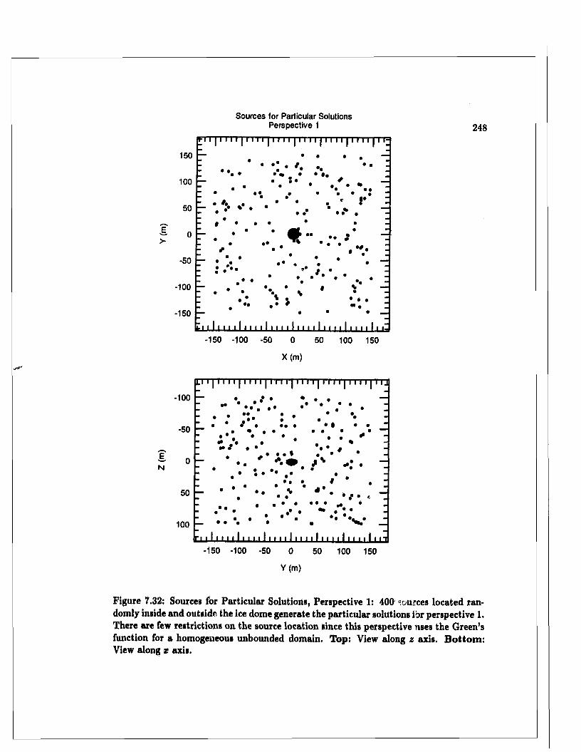
Sources for Particular SolutionsPerspective 1 248
150
• • •• *100
• •• •
• •
E,> • •
• • •#-50
• •
-100
••-150
150 -100 -50 0 50 100 150
X ( m )
-100• •
• •• • •-50
m i0
50
100t i l
-150 -100 -50 0 50 100 150
Y(m)
Figure 7.32: Sources for Particular Solutions, Perspective 1: 400 sources located randomly inside and outside the ice dome generate the particular solutions ibr perspective 1. There are few restrictions on the source location since this perspective uses the Green’s function for a homogeneous unbounded domain. Top: View along z axis. B ottom : View along z axis.
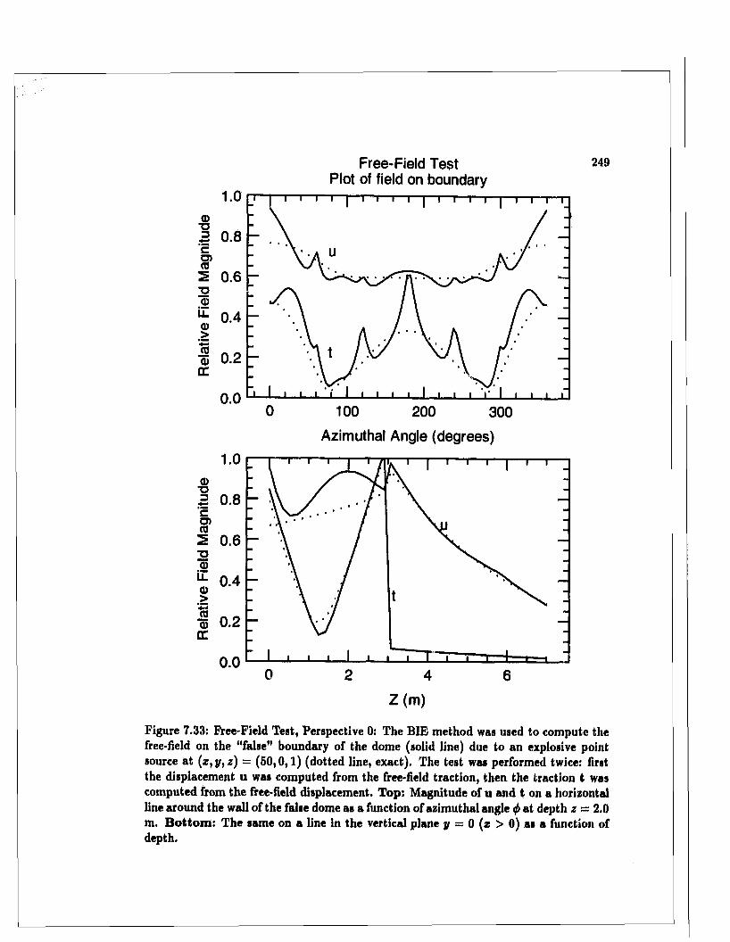
0)T3D
2<1)i i©>J20)tr
Free-Field TestPlot of field on boundary
i — |— i— i— i— i— |— !— i— i— r
249
i — i— i— r
2 0.8 ~
cS'2 0.6 -
0.4 -
■S 0 .2
0 o Lj— 1— 1— 1— 1— i— I 1— 1 1 1 I 1 1 1 ■* I 1 1 10 100 200 300
Azimuthal Angle (degrees)
a)T3 2 0.8 cS'5 0.62a)E 0.4 ©>iS _ _ 0) 0.2 IT
0.0
Z (m )
Figure 7.33: Free-Field Test, Perspective 0: The BIE method was used to compute the free-field on the “false” boundary of the dome (solid line) due to an explosive point source at (x, y, z) = (50,0,1) (dotted line, exact). The test was performed twice: first the displacement u was computed from the free-field traction, then the traction t was computed from the free-field displacement. Top: Magnitude of u and t on a horizontal line around the wall of the false dome as a function of azimuthal angle ^ at depth z = 2.0 m. B ottom : The same on a line in the vertical plane y = 0 (a > 0) as a function of depth.
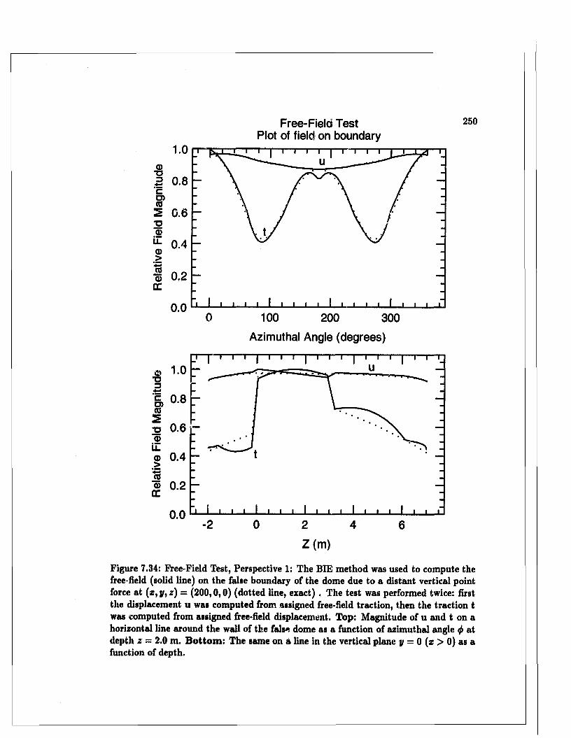
Free-Field TestPlot of field on boundary
1.0
TJ 3 0.8 'cS’2 0.6
0.4
0.2
0.0100 200
Azimuthal Angle (degrees)
300
© ■
<022 0.6g>
Ll© 0.4 >IS©£E
0.2
0.0
Z (m)
Figure 7.34: Eree-Field Test, Perspective 1: The BIE method was used to compute the free-field (solid line) on the false boundary of the dome due to a distant vertical point force at (x , y, z) = (200,0,0) (dotted line, exact) . The test was performed twice: first the displacement u was computed from assigned free-field traction, then the traction t was computed from assigned free-field displacement. Top: Magnitude of u and t on a horizontal line around the wall of the false dome as a function of azimuthal angle <f> at depth z = 2.0 m. B ottom : The same on a line in the vertical plane y = 0 (x > 0) as a function of depth.
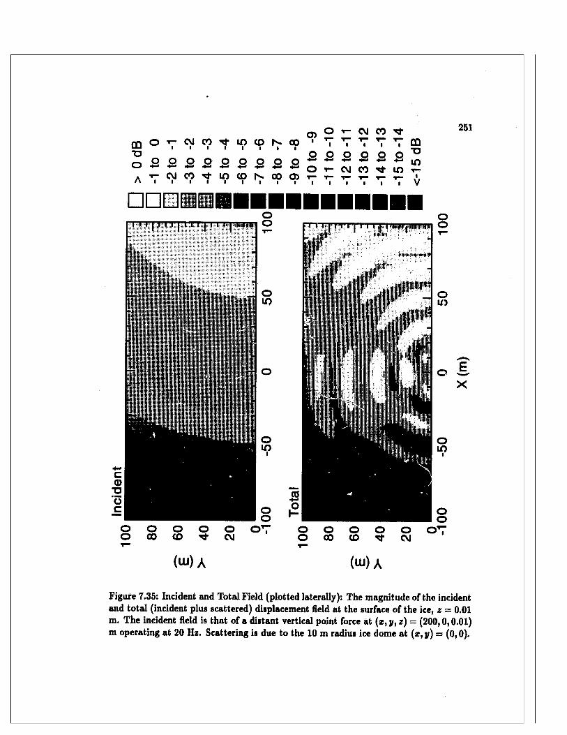
05 O y— CM COC Q O T - c v J c o ^ i n c o r ^ o o ' T V T V V mI I I I I | | | MMT3 O O O O O O ^^ o o o o o o o o o ^ ^ ^ ^ - ^ - ^ i o
A T - C V I C O ^ l O O S C O a i - T - r - r - i - T - 'a i i i i i i i ■ i i i i i | , v
251
TTT
:/ ifll/'-;';-' i" '
J 0
X
( w ) A (w) A
Figure 7.35: Incident and Total Field (plotted laterally): The magnitude of the incident and total (incident plus scattered) displacement field at the surface of the ice, z — 0.01 m. The incident field is that of a distant vertical point force at (z, y, z) = (200,0,0.01) m operating at 20 Hz. Scattering is due to the 10 m radius ice dome at (z, y) = (0,0).
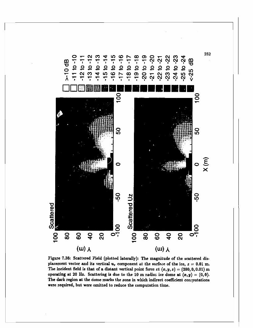
O 1 - CM CO ^ i n CDCD■OoT “IA
Io
I IQ o
IO
Io
T - CVJ CO T f lO CO
oh -
N C O O O i - C V l C O ’t t - t— i — C V J C V J C M C M C V l C QI I I I I I I I -0O O O Q O O O O-I— > - * - ' ■ £ 5
QOcno-<-c\ ioo'^-Lnc\ j1 - T - CM CM CVI CM 0 4 CM i i i ■ i i i i V
252
□□□
(w ) A (ui) AFigure 7.36: Scattered Field (plotted laterally): The magnitude of the scattered displacement vector and its vertical uz component at the surface of the ice, z — 0.01 m. The incident field is that of a distant vertical point force s,t (x, y, z) = (200,0,0.01) m operating at 20 Hz. Scattering is due to the 10 m radius ice dome at (* ,y) = (0,0). The dark region at the dome marks the zone in which indirect coefficient computations were required, but were omitted to reduce the computation time.
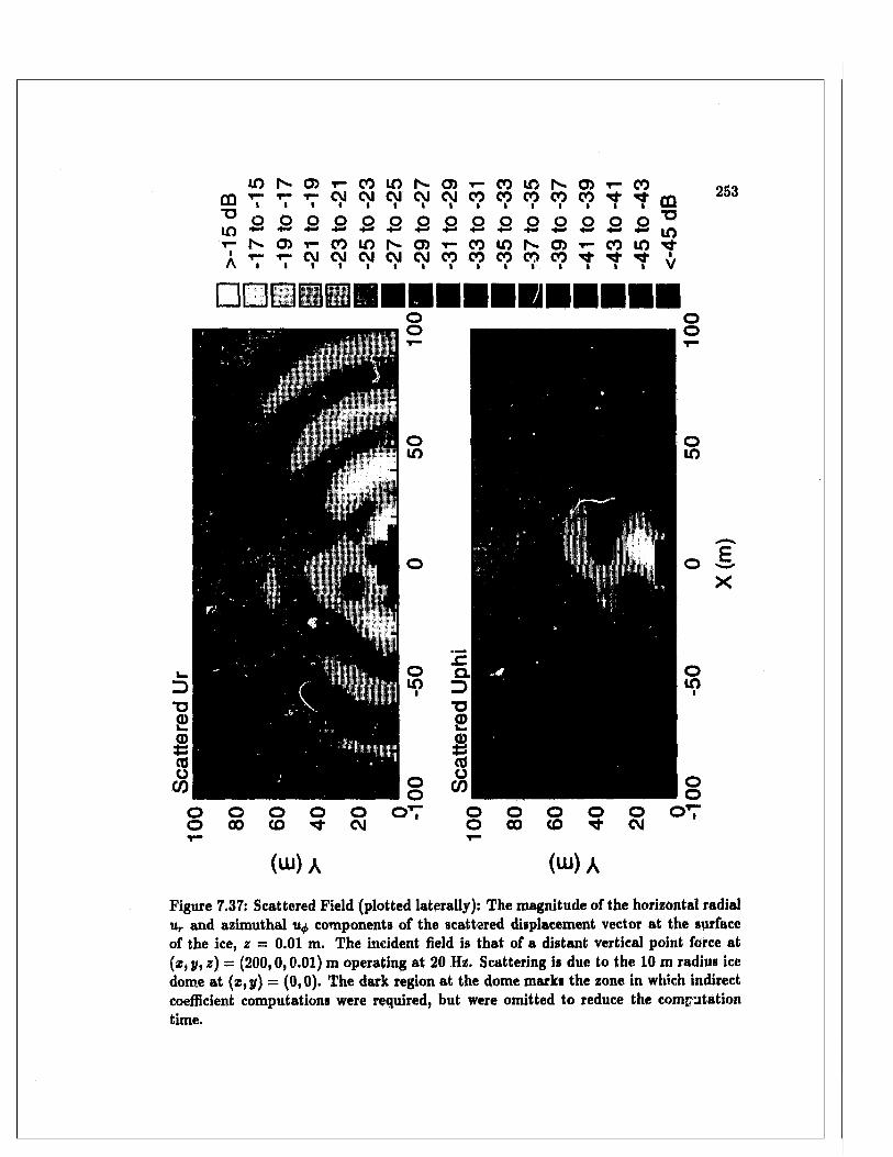
CD"Uin■t—
■
A
i n N O ) T - o o i o N o > T - c o m N ®t- t- t- C M C M C M C M C M C O C O C O C O C O Tf-I
CO
O O Q O O O O O O O O O O O O
N f f i r C O l f l N f f l T - n i O S O )t- ^ C M C M C M C M C M C O C O C O C O C O
■ ■ ■ ■ ■ ■ ■ E lI
co in
CD■oinV
253
k■D£
$COo
CD
■ 111oin
o o o o o O 00 <0 Tf CM
o o
O T
E,X
o o o o O T00 CO Tf CM
(w)A (w)A
Figure 7.37: Scattered Field (plotted laterally): The magnitude of the horizontal radial ur and azimuthal components of the scattered displacement vector at the surface of the ice, z = 0.01 m. The incident field is that of a distant vertical point force at (x, y, z) — (200,0,0.01) m operating at 20 Hz. Scattering is due to the 10 m radius ice dome at (* ,y) = (0,0). The dark region at the dome marks the zone in which indirect coefficient computations were required, but were omitted to reduce the computation time.
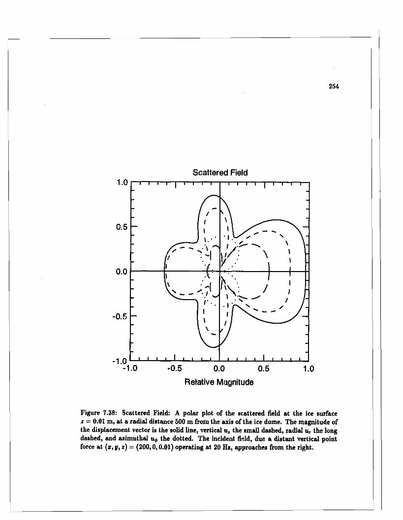
254
Scattered Field
0.5
0.0
-0.5
- 1.0- 1.0 -0.5 0.0 0.5 1.0
Relative Magnitude
Figure 7.38: Scattered Field: A polar plot of the scattered field at the ice surface z - 0.01 m, at a radial distance 500 m from the axis of the ice dome. The magnitude of the displacement vector is the solid line, vertical uz the small dashed, radial ur the long dashed, and azimuthal u<j, the dotted. The incident field, due a distant vertical point force at (z ,y ,z ) = (200,0,0.01) operating at 20 Hz, approaches from the right.
255
C h a p t e r 8
Conclusions
I have followed two paths towards a three-dimensional scattering model for layered
media. The first followed Huygens’ principle, which lead to a physical interpretation of the
BIE m ethod in term s of wavelet superposition, then to an indirect method for computing
troublesome integral coefficients using particular solutions in the absence of scattering, and
finally to several num erical tests for every application of the BIE m ethod the consistency,
free-field and null-field tests. The second followed the schematic diagram for layered media,
which first lead to the scattering m atrix m ethod for cylindrical waves, then to the channel
m atrix and SVD m ethod for carrying out an exhaustive search for norm al modes th a t was
implemented by th e SAM PLE program , which in turn lead to some discoveries regarding
modes. The two paths met in a three-dimensional scattering model for layered media
When faced with a complicated model, we m ust ask whether the same results could
be achieved in a simpler way. I believe there is ju st one minor point in which the present
model m ight have been simplified, and th a t is by limiting the problem to a single scattering
inclusion ra ther th a n generalizing to m ultiple inclusions. As it happened, com puter limi
tations on the num ber of boundary elements discouraged me from attem pting the multiple
body problem here. Beyond this, fu rther simplifications could only be made by sacrificing
one of the three features I set out to include form the beginning; by simplifying as others
have done, using strictly fluid m edia instead of layered elastic media, im penetrable inclu
sions instead of penetrable, or two dimensions instead of three. Each step towards greater
CHAPTER 8. CONCLUSIONS 256
realism engenders greater complexity in the model. There is no escape from this general
rule of modeling.
The main developments made in the course of this work are summarized below.
8.1 C onclusions regarding layered m edia
The elastic field due to a general class of seismic point sources, some of which
are not axially symmetric, was derived here for arb itrarily layered m edia in term s of the
Fourier-Bessel transform . This topic has been covered by others in geophysics, and to a
lesser ex ten t in ocean acoustics, bu t my own contribution has been to
1. bring together fluid and solid m edia in a single comprehensive analysis;
2. press the analysis to completion, to give all nine components of the field— three com
ponents of displacement, and six of stress— as required by the BIE m ethod;
3. develop a schematic ladder diagram for layered media, based upon the numerically
stable scattering m atrix m ethod for two-port networks;
4. develop a robust norm al mode search routine which, under the direction oi the user,
can perform an exhaustive search for modes in the complex plane.
The upshot of these advances are reviewed below.
8.1.1 Schem atic ladder diagram
By treating the waveguide as a linear system whose components and interaction
are easy to visualize and understand, the schematic ladder diagram forms a conceptual
bridge between the physics of cylindrical or plane waves in layered media, and the more
abstract m atrix operations needed to com pute the field due to a point source. Indeed, the
diagram resembles the schematics an engineer m ight use to analyze a linear system , and the
corresponding m atrix can be w ritten directly by inspection. The scattering m atrix m ethod
a t the h ea rt of the diagram is an extension of K ennett’s numerically stable recursive scheme
I W ____________________________'T he schem atic diagram was developed step by step in Chapter 4, beginning in Section (4.2).

CHAPTER 8. CONCLUSIONS 257
8.1.2 Normal m odes and SVD
A mode occurs a t frequencies u and horizontal slownesses p a t which the global
m atrix representing vertical propagation of cylindrical (or plane) waves through the layers is
singular.2 The smallest singular value w\ of the global m atrix was used as the m ode search
function, for the zeros of indicate singularity. To speed up the search for roots, the
dimensions of the global m atrix were compressed to give the channel m atrix, in a way that
ensures th a t the search remains sensitive to modes trapped at any dep th in the waveguide.
The m ain advantages of using uti as the search function are tha t
1. SVD is a robust m atrix operation for nonsingular and singular matrices alike;
2. SVD gives th e (un-normalized) vertical m ode function for a mode;3
3. the second smallest singular value w2 can be used to identify and resolve uncommonly
close mode pairs (double roots) th a t can occur when the waveguide supports two
weakly coupled sound channels.4
Using still other singular values in the search, the method could also be extended to check
for close mode trip lets and so forth , in the rare event th a t the waveguide supports throe or
more modes in as m any sound channels a t virtually the same w and p.
8.1.3 The m ode search program SAM PLE
A channel m atrix and SVD m ethod for the mode search was implemented in a
program called SAM PLE, which undertakes the mode com putations needed for the rigorous
demands of the B IE m ethod. Under the direction of the user, SAM PLE can perform an
exhaustive search for all of the different types of modes th a t occur in layered media: whether
P-SV or SH, propagating or evanescent, trapped or leaky, proper or improper (found on
various Riemann sheets), or duct or interface modes. SAMPLE furtherm ore computes all
nine components of the elastic wave field (ur , u^„ uz , r TT, r r,/„ ttz , r,/,z, rzz) due to a class of
2Section (5.2).3Section (5.2.1),^Section (5.3,3).
CHAPTER 8. CONCLUSIONS 258
seismic point sources comprising general point forces, and couples with and w ithout moment.
The proper mode series is a complete representation of the field in a bounded waveguide. By
including a long series of evanescent modes in a bounded waveguide, SAM PLE can com pute
the field very close to an ideal point source, within a small fraction of a wavelength, and
th a t is essential for the BIE m ethod.
SAM PLE includes m any utilities th a t make it an excellent tool for the analysis
of modes. It plots the location of modes and E JP branch lines in the complex slowness or
wavenumber plane, plots vertical mode functions, computes group velocity, tracks modes
with changing frequency, computes vertical energy flux in a m ode function, and sorts modes
in a num ber of useful ways. It also incorporates three im portan t tests for mode com puta
tions:
1. verification . each mode using Rayleigh’s principle;5
2. verification of part or all of the mode series using contour integration and the residue
theorem ;6
3. and verification of the dom inant modes in the medium to far field the spectral E F T —a
special form of contour integration.7
Further possib ilities for SA M PLE
The following additions to SAM PLE may prove helpful:
1. Airy functions: SAM PLE now supports homogeneous solid and fluid layers. A nother
possibility for fluid layers is to make the square of the phase slowness for P waves vary
linearly with depth in a layer, for which the vertical propagation is governed by Airy
functions [66, sect. 2.5.1]. In this way, the sound speed profile in the w ater column
can be approxim ated using fewer layers for greater program efficiency.
2. Pekeris branch cuts: SAMPLE now uses the E JP branch cuts when com puting ver
tical slowness,8 but the Pekeris cuts (extending vertically from the branch point) are
5See Section (5.4.4).“See Section (5.4.2),7See Section (5.8),"Sec Fig. (4.1).
CHAPTER 8. CONCLUSIONS 259
convenient for leaky mode environm ents, when the search is liable to cross the E.1P
cuts several times [125]. They could be included as an option in SAMPLE.
3. Im proper m ode norm alization: A lthough SAMPLE can find improper modes, it can
not use them in the mode series because the integral identities used to normalize a
m ode function have only been implemented for proper modes. Im proper modes could
be normalized using modified integral identities.9
4. Optim ization: As with most modeling programs in the development stage, SAMPLE
could be optimized using specialized com putation routines. In particular, an SVD
routine for banded matrices m ay speed up the mode search for waveguides having
m any channels.
5. Anisotropy: Following the m ethod of Takeuchi and Saito [122] it is possible to include
anisotropy in the solid layers, where the phase speeds for waves travelling' horizontally
are different from waves travelling vertically.
Items 2 and 3 above are never needed for bounded waveguides because they do
not have im proper modes.
8.1.4 The properties of m odes
SAM PLE m ade it possible to investigate modes in great detail, revealing little-
known properties of modes th a t are of interest in their own right. Those properties are
summarized below.
Upward energy flow from an infinite halfspace
Modes in infinitely deep waveguides sometimes carry energy upwards from depths
below all sources and reflecting interfaces.10 This apparent contradiction to the radiation
condition is actually an energy loss m echanism for the vibrations of waves trapped in the
basement media, when the ra te ol decay of the mode due to energy loss exceeds the P or S
aSee note regarding improper mode normalization on page 167,,0Section (6,1.4).
CHAPTER 8. CONCLUSIONS 260
wave absorption ra te in the bottom. The upward flow is slight, but it m ay be the cause of
alarm to the conscientious modeler.
Proper leaky modes
It is generally assumed tha t leaky modes in unbounded waveguides m ust be im
proper modes whose vertical mode functions grow exponentially with depth. B ut leaky
modes radiating into a lossy infinite half space may also be proper modes, with m ode func
tions th a t decay with dep th .11 This happens when the exponential vertical decay due to
absorption overcomes the exponential growth characteristic of leaky modes in lossless me
dia T he shear wave absorption used to model ocean sediments is often enough to make
S-leaky modes proper.
Proper leaky modes are of interest for modeling purposes, since norm al mode
programs designed for proper modes with complex horizontal slowness should be able to
handle proper leaky modes w ithout modification. A t times it m ay be justified to add
artificially high absorption in the basement to make a leaky mode environm ent amenable
to a proper mode program.
Radiation modes in deep bounded waveguides
A waveguide having a deep bounded basement layer is often used to model the
corresponding unbounded case. Since the basement layer is thick, there is a proliferation of
radiation modes close to the P and S branch lines.12 T he range of good agreem ent between
the two was estim ated in Section (6.4). It was also shown th a t isolated radiation modes
in an unbounded waveguide approxim ate the dom inant leaky modes of the corresponding
unbounded waveguide.
R ayleigh m ode o f the second kind
I t was shown th a t a leaky interface mode can be trapped a t the rigid boundary in
welded contact with a solid layer. This mode can appear as a proper m ode in deep bounded
11 Section (6.2,1),'^Section (6.2,2).

CHAPTER 8. CONCLUSIONS 261
waveguides, when a thick solid basement layer is bounded by a rigid interface.13
8.2 T he indirect BIE m ethod
The indirect BIE m ethod infers numerically troublesome integral coefficients from
many particu lar free-field solutions of the boundary integral equations needed for the in
tended scattering problem .1'1 The m ain advantages of the indirect method are that:
1. it makes the BIE method possible in layered media when the Green’s function is
com puted using mode sum m ation, for there is presently no other way to avoid poor
convergence of the m ode series at the close ranges routinely encountered in the BIE
m ethod;
2. all troublesome integral coefficients are treated in the same way, whether troublesome
due to the singularity in the surface-ficld equation, poor convergence in the Green’s
function, or for any other reason.
In addition, the indirect BIE m ethod includes features th a t could be included in
any BIE m ethod for scattering. Most im portant are the three tests it supports:
1. the free-field test, which is a comprehensive test of all aspects of the HIE method for
each application;15
2. the null-field test, which tests the boundary field computed by the BIE m ethod;10
3. the consistency test, which verifies th a t the integral coefficients for a boundary integral
equation have been accurately computed a t the time of com putation .17
Of secondary im portance is its unprecedented flexibility, for the new m ethod permits
13Section (6,2,3).HT he new indirect BIE method was first described in Chapter 3, then applied to layered media in Chapter
7,ls See Section (5,4,2),10Scction (3,7),17Scction (3,3),
CHAPTER 8. CONCLUSIONS 282
1. any combination of surface-field and null-field equations when determ ining the bound
ary fields;
2. any number .>f surface-field com putation points, placed anywhere on the boundary,
rather than ju st a t the element nodes;
3. multiple penetrable, im penetrable and actively vibrating inclusions;
4. lines of discontinuity in the field; in the displacement field where the inclusion crosses
an interface with a fluid layer, or in the traction at an edge on the boundary,
By experim enting with the num ber of com putation points and their location, it is sometimes
possible to improve the numerical stability of the BIE solution.
The main disadvantage of the m ethod is th a t it is com putationally intensive. Many
particular solutions are needed to infer troublesome coefficients indirectly, and in layered
media, com puting the particular solutions a t the boundary element nodes takes considerable
time, making it best to com pute and save them for ready access. This of course increases
the compu ter disk space used by the model. To judge how slow (or fast) the indirect m ethod
may be relative to other three-dimensional BIE m ethods for layered media, we m ust wait
until alternative models are developed.
8.2.1 Future research
The next step is to use the new model to explore general principles of scattering,
by applying it to particular instances of scattering. To say, for example, when and to what
degree scattering from a series of ice keels is a significant loss mechanism for long range
propagation in the Arctic ocean, or whether Scholte modes could be used to detect objects
buried in the sea floor. T he model could also be used in the development of faster approx
imate trea tm ents of scattering, along the lines of the Kirehhoff or Born approxim ations,
T he model itself could be improved by
1. making provisions for the com putation of the scattered stress field, especially the
normal stress in fluids commonly used in ocean acoustics;18
'"Section (3.2.5).
CHAPTER 8. CONCLUSIONS 263
2. perm itting layered m edia inside a penetrable inclusion as well as outside;
3. testing its use with m ultiple scattering inclusions;
4. conducting a thorough analysis of the continuity conditions for lines of discontinuity
on the boundary: edges and interfaces between layers;
5. and by a theoretical analysis into the stability of integral equations tha t are both of
the first and second kind.19
8.3 C losing Rem arks
I close on a cautionary note for modelers. The BIE method for scattering, whether
or not the indirect method described here is used, supports several excellent tests: the
consistency test, null-field test, and especially the free-iield tests. In numerical modeling
it is rare to have such comprehensive tests available. All three tests for the BIE m ethods
have been reviewed here, though the null-field and free-field tesla have appeared elsewhere
in the literature . I t would appear, however, th a t such tests have rarely been used to verify
results published in the literature, probably because the tests are little known. I find that
worrisome, for my own experience has been th a t it is not enough to prove the BIE method
by successfully solving a problem th a t others have solved another way, Rather, every
application of the BIE m ethod must be tested because changes in the boundary, frequency,
elastic media, and boundary conditions, invite a host of difficulties th a t m ay lie quiescent
in a benchmark test. This is particularly true for scattering in layered media, The tests do
not require much ex tra effort, provided they have been included in the overall plan for the
BIE model from the outset.
' “Section (2.7).
Bibliography
[1] Aki, K., and P.G. Richards, Quantitative seismology, Vol. 1, Freeman, San Fran-
sisco (1980).
[2] Abramowitz, M., and I.A. Stegun, Handbook o f M athematical Functions, Na
tional Bureau of S tandards, Applied M athem atics Series 55, W ashington DC (1965).
[3] Aliabadi, M.H., W.S. Hall, and T.G. Phemister, “Taylor expansions for sin
gular kernels in the boundary element m ethod,” International Journal fo r Numerical
Methods in Engineering, 21, (1983): 2221-2236.
[4] Arfken, G., M at:> matical methods fo r physicists, T hird Ed., Academic Press,
Toronto (1985).
[5] Arvelo, J.I., M. Talmant, and H. Uberall, “A norm al m ode model of under
w ater propagation including shear effects in a layered ocean floor,” Com putational
Acoustics, 3 (1990): 131-150.
[6] Auld, B.A., Acoustic fields and waves in solids, Vol. 1, John Wiley and Sons (1973).
[7] Baker, B.B., and E.T. Copson, A mathematical theory o f H uygens’ principle, 2nd
ed., Oxford a t the Claredon Press (1949).
[8] Banerjee, P.K., and R. Butterfield, Boundary element methods in engineering
science, McGraw-Hill, M aidenhead, Brekshire, England (1981).
BIBLIOGRAPHY 265
[9] Bartberger, C,, '''’Normal mode solutions and computer programs fo r underwater
sound propagation,” P a rt II-Prog. for A rbitrary Velocity Profiles, Naval Air Develop
m ent Center, Report No. NADC-72002-AE (April 4 1973).
[10] Batchelor, G.K., A n introduction to flu id dynamics, Cam bridge University Press
(1967).
[11] Benthien, G.W., and D. Barach, CHIEF user’s manual, Naval Ocean Systems
C enter, San Diego, California, NOSC TD 970 (Feb 1987).
[12] Bhatia, A.B., “Ultrasonic Absorption,” Dover Publications, New York (1985).
[13] Bhatia, A .B., and R .N . Singh, Mechanics o f deformable media, Adam llilger,
B ristol (1986).
[14] Bolt, B.A., Editor, Seismic surface waves, in Methods in computational physics, vol.
11, Academic Press, New York (1972).
[15] Brebbia, C.A., J.J. Rego Silva, and P.W. Partridge, C hapt. 2 Com putational
Form ulation, in Boundary element methods in acoustics, ed. R.D. Ciskowski and (I,A.
B rebbia, co-pubiished by C om putational Mechanics Publications, Southam pton, and
Elsevier Science Publishers L td., New York (1991).
[16] Brekhovskikh, L ., Waves in layered media, 2nd ed., Academic Press, New York
(1980).
[17] Brekhovskikh, L., and Y. Lysanov, Fundamental ocean acoustics, Springer-Verlag,
Berlin (1982).
[18] B ro o k e , G .H ., a n d J .M . O z a rd n-situ measurements of elastic properties of sea
ice,” U nderw ater acoustic d a ta processing, Ed. Y.T. Chan (1989): 113-118.
[19] Burns, D.R., and R.A. Stephen, “Three-dimensional numerical modeling of geoa
coustic scattering from seafloor topography,” Journal o f the Acoustical Society of
America, 88 (1990): 2338-2345.
BIBLIOGRAPHY 266
[20] Burns, D.R., “Acoustic and elastic scattering from seamounts in three dimensions—
a numerical study,” Journal o f the Acoustical Society o f America, 92 (1992): 2784-
2791.
[21] Burridge, R., and L. Knopoff, “Body force equivalents for seismic dislocations,”
Bulletin o f the Seismological Society o f Am erica, 54 (1964): 1875-1888.
[22] Burton, A.J., “T he solution of Helm holtz’ equation in exterior domains using in te
gral equations” , National Physical Laboratory, Report NAC 30 (January 1973).
[23] Byron F.W ., and R.W. Fuller, M athematics o f classical and quantum physics,
Dover Publications, New York (1969).
[24] Chew, W.C., “ Waves and fields in inhomogeneous media,” Van N oslrand Reinhold,
New York (1990).
[25] Chin, R.C., G.W. Hedstrom and L. Thigpen, “M atrix m ethods in synthetic
seismograms,” Geophysical Journal o f the Astronomical Society, 77 (1984): 483-502.
[26] Chin-Bing, S.A. , D. B. King, and J. D. Boyd, “T he effects of ocean environ
mental variability on underw ater acoustic propagation forecasting,” in Oceanography
and acoustics, Ed. A. R. Robinson and D. Lee (1994).
[27] Ciskowski, R.D. and C.A. Brebbia, Editors, Boundary element methods in acous
tics, C om putational Mechanics Publications, Elsevier Applied Science, London (1991).
[28] Clay, C.S., and H. Medwin, Acoustical oceanography: principles and applications,
John Wiley and Sons (1977).
[29] Colton, D., and R. Kress, Integral equation methods in scattering theory, John
Wiley and Sons (1983).
[30] Dawson, T.W., “The D REP internal wave normal m ode model - theoretical back
ground,” Technical M emorandum 88-7, Defence Research Establishm ent Pacific, Es
quim au, C anada (1988).

BIBLIOGRAPHY 267
[31] Dawson, T.W ., and J.A. Fawcett, “A boundary integral equation method for
acoustic scattering in a waveguide with nonplanar surfaces,” Journal o f the Acoustical
Society o f America, 87 (1990): 1110-1124.
[32] Dawson, T.W ., “Scattering m atrix and boundary integral equation methods for
long range propagation in an acoustic waveguide with repeated deform ations,” Journal
o f the Acoustical Society o f America, 90 (1991): 1560-1574.
[33] Dawson, T.W ., “Scattering m atrix and boundary integral equation methods for
acoustic propagation over a slope,” Journal o f the Acoustical Society o f America, 90
(1991): 1575-1581.
[34] Dawson, T.W ., “Acoustic scattering in a three-dimensional oceanic waveguide using
boundary integral equation m ethods,” Journal o f the Acoustical Society o f A merica,
90 (1991): 2609-2622.
[35] Dawson, T.W ., and R.T. Kessel, SAM PLE: A Seismo-Acoustic Mode Program
fo r Layered Environments. Theoretical Background, Defence Research Establish men t
A tlantic (C anada) Technical M emorandum D R E A /T M /95/225 (October 1.995).
[36] DeSanto, J.A., Scalar wave theory, Green’s functions and applications, Springer*
Verlag, Berlin (1992).
[37] Diachok, O.S., “Effects of sea-ice ridges on sound propagation in the Arctic Ocean,”
Journal o f the Acoustical Society o f America, 59 (1976): 1110-1120.
[38] DiNapoli, F.R. and R.L Davenport, “Numerical models of underwater acoustic
propagation,” C hapter 3 in Ocean Acoustics, Topics in C urrent Physics, Volume 8,
E dited by J.A . DeSanto, Springer*Verlag, Berlin (1979),
[39] Doornbos, D.J., ed., Seismological Algorithms: com putational methods and com
pu ter program s, Academic Press, London (1988).
[40] Dougherty, M.E., and R.A. Stephen, “Geoacoustic scattering from sealloo, fea
tures in the ROSE area,” Journal o f the Acoustical Society o f America, 82 (1987):
238-256,
BIBLIOGRAPHY 268
[41] E liseevnin , V .A ., and Y .I. Tuzhilkin, “Diffraction of a sound field a t a plane
rectangular vertical screen in a waveguide,” Acoustical Physics, 41 (1995): 214-218.
[42] E llis, D .D ., and M .F . C hapm an, “A simple shallow water propagation model
including shear wave effects,” Journal o f the Acoustical Society o f America, 78 (1985):
2087-2095.
[43] E tter , P .C ., Underwater acoustic modeling: principles techniques and applications,
Elsevier Science Publishers (1991).
[44] E w ing, W .M ., W .S . Jardetsky and F. Press, Elastic waves in layered media,
McGraw-Hill, New York (1957).
[45] Evans, R .B ., “A coupled m ode solution for propagation in a waveguide w ith step
wise depth variations of a penetrable bottom ,” Journal o f the Acoustical Society o f
Am erica, 74 (1983); 188-195.
[46] Faw cett, J .A ., and T .W . D aw son, “Fourier synthesis of three-dim ensional sca tte r
ing in a two-dimensional oceanic waveguide using boundary integral equation m eth
ods” , Journal of the Acoustical Society o f America, 88 (1990): 1913-1920.
[47] Ficke, J .R ., “Acoustic scattering from elemental Arctic ice features: numerical model
resu lts,” Journal o f the Acoustical Society o f America, 93 (1993): 1784-1796.
[48] Frisk, G .V ., Ocean and seabed acoustics, a theory o f wave propagation, Prentice Hall,
New Jersey (1994).
[49] G ilbert, F ., and G .E . Backus, “Propagator matrices in elastic wave vibration
problems,” Geophysics, Vol. 31 (1966): 326-332.
[50] G erstoft, P ., and H . Schm idt, “A boundary element approach to ocean seisinoa-
coustic facet reverberation,” Journal o f the Acoustical Society o f America, 89 (1991):
1629-1642.
[51] Graff, K .F ., Wave m otion in elastic solids, Dover Publications, New York (1975).
BIBLIOGRAPHY 269
[52] M. Guiggiani and A. Gigante, “A general algorithm for m ultidimensional Cauchy
principal value integrals in the boundary element m ethod,” Transactions of the ASME,
57 (1990): 906-915.
[53] Guiggiani, M., “Com puting principle-value integrals in 3-D BEM for time harmonic
elastodynam ics - a direct approach,” Communications in Applied Numerical Methods,
8 (1992): 141-149.
[54] Hamilton, E . L ., “Geoacoustic modeling of the sea floor” , Journal o f the Acoustical
Society o f Am erica, 68 (1980): 1313-1340.
[55] Harkrider, D.G., “Surface waves in multi-layered elastic media I: Rayleigh and hove
waves from buried sources in a m ultilayered halfspace,” Bulletin o f the Seismological
Society o f Am erica, 51 (1964): 627-679.
[56] Haskell, N .A ., “The dispersion of surface waves on multilayered media,,” Bulletin o f
the Seismological Society o f Am erica, 43 (1953): 17-34.
[57] Haskell, N .A., “Radiation p a tte rn of surface waves from point sources in a m ulti
layered m edium ,” Bulletin o f the Seismological Society o f America, 54 (1964): 377-393.
[58] H e ise , U., “The calculation of Cauchy principal values in the integral equations for
boundary value problems of the plane and three-dimensional theory of elasticity,”
Journal o f Elasticity, 5 (1975): 99-110.
[59] Heppenheimer, T.A., Anti-subm arine warfare: the threat, the strategy, the solu
tion, Pasha Publications Inc., Arlington (1989).
[60] Hudson, J.A ., “A quantitative evaluation of seismic signals as toleseismic distances
- R adiation from point sources,” Geophysical Journal o f the Astronomical Society, IK
(1969): 233-249.
[61] Hudson, J.A ., The excitation and propagation o f elastic waves, Cam bridge Univer
sity Press, C am bridge (1980).
BIBLIOGRAPHY 270
[62] H u y g e n s , C ., Treatise on Lights trans. S P. Thom pson, in G reat Books of the W est
ern World, Volume 34, Encyclopedia B ritannica, Chicago (1952).
[63] Ingenito, F., “Scattering from an object in a stratified m edium ,” Journal o f the
Acoustical Society o f America, 82 (1987): 2051-2059.
[64] Jackson, J.D., Classical Electrodynamics, John Wiley and Sons (1975).
[65] Jensen, F.B., and M.C. Ferla, ‘lSN A P : The S A C L A N T C E N normal mode acoustic
propagation model,” SACLANT ASW Research Center, La Spezia, Italy, January 15
(1979).
[66] Jensen, F.B., W.A. Kuperman, M.B. Porter and H, Schmidt, Computational
ocean acoustics, American Institu te of Physics Press, New York (1994).
[67] Kawase, H., “Time dom ain response of a semi-circular canyon for incident SV, P and
Rayleigh waves calculated by the discrete wavenumber boundary element m ethod,”
Bulletin o f the Seismological Society o f America, 78 (1988): 1415-1437.
[68] K e llo g g , O.D., Foundations o f potential theory, Dover Publications (1953).
[69] Kennett, B.L.N., and N.J. Kerry, “Seismic waves in a stratified halfspace,” Geo
physical Journal o f the Astronom ical Society, 57 (1979): 557-583.
[70] Kennett, B.L.N., “Elastic wave propagation in stratified m edia,” in Advances in
Applied Mechanics, Vol. 21, ed., C.S. Yih, Academic Press, New York (1981).
[71] Kennett, B.L.N., Seism ic wave propagation in stratified media, Cam bridge Univer
sity Press, Cambridge (1983).
[72] Kerry, N.J., “Synthesis of seismic surface waves,” Geophysical Journal o f the A stro
nomical Society, 64 (1981): 425-446,
[73] K e sse l, R.T., “The exterior Helmholtz integral equation and its approxim ate solu
tion for acoustic radiation problems,” M aster’s Thesis, Dept, of Physics, University
of W aterloo, O ntario (1989).

BIBLIOGRAPHY 271
[74] Kim, J.S., Radiation from directional seismic sources in laterally stratified media
ivith application to Arctic ice cracking noise, PhD Thesis, M assachusetts Institu te of
technology (M ay 1989).
[75] Korneev, V.A., and L.R. Johnson, “Scattering of elastic waves by a spherical
inclusion - I ,” Geophysical Journal International, 115 (1993): 230-250.
[76] Kress, R., Linear integral equations, Springer Verlag, New York (1989).
[77] Kuo, J.T., “The influence of the elasticity of the bottom on wave propagation,” (loin*
putational Acoustics: Wave Propagation, D. Lee, ll.L . Strcnberg, and M.H. Schultz
Editors, Elsevier Science Publishers B.V. (1988).
[78] Kupradze, V.D., Potential methods in the theory o f elasticity, trans. 11. Gutl'reund,
ed. I. Meroz, Isreal Program for Scientific Translations, Monsou, Jerusalem (1965).
[79] Lachat, J.C., and J.O. Watson, “Effective numerical treatm ent of boundary inte
gral equations: a formulation for three-dimensional elastostatics,” International Jour
nal fo r Numerical Methods in Engineering, 10 (1976): 991-1005.
[80] Levinson, S.J., E,K. Westwood, R.A. Koch, S.K. Mitchell, and C.V. Shep
pard, “An efficient and robust m ethod for underw ater acoustic normal-mode com pu
tations,” Journal o f the. Acoustical Society o f America, 97 (1995): 1576 1585,
[81] Lighthill, M. J., Waves in fluids, Cambridge University Press, Cambridge (1978)
[82] Lim, R., J.L. Lopes, R.H. Hackman, and D.G. Todoroff, “Scattering by ob
jects buried in underw ater sediments: theory and experim ent,” Journal of the Acous
tical Society o f America, 93 (1993): 1762-1783.
[83] Love, A. E. H,, A treatise on the mathematical theory o f elasticity, 4tii ed,, Dover
Publications, New York (1944).
[84] L u , I .T . , L .B . F e lsen a n d A .H . K a m e l, “Eigonreverberations, eigenmodes and
hybrid combinations: a new approach to propatton in layers multiwave media” , Wave
M otion, 6 (1984): 435-457.
BIBLIOGRAPHY 272
[85] Lu, I.T., and L.B. Felsen, “Ray, mode, and hybrid combinations for source-excited
propagation in a elastic p late ,” Journal o f the Acoustical Society o f America, 78
(1985): 701-704.
[86] Lu, I.T., “Analysis of acoustic wave scattering by scatterers in layered m edia using
the hybrid ray-mode (boundary integral equation) m ethod,” Journal o f the Acoustical
Society o f Am erica, 86 (1989): 1136-1142.
[87] Manolis, G.D., “A com parative study on three boundary element m ethod ap
proaches to problems in elastodynam ics,” International Journal fo r Numerical M eth
ods in Engineering, 19 (1983): 73-91.
[88] Manolis, G.D. and D.E. Beskos, Bounday element methods in elastodynamics,
Unwin Hyman, London, (1988).
[89] Marschall, R.A., “B oundary element solution of a body’s exterior acoustic field near
its internal eigenvalues,” Journal of Com putational Acoustics, 3 (1993): 335-353.
[90] Miklowitz, J., The theory o f elastic waveguides, Paperback Edition, North-Holland,
Am sterdam (1984).
[91] Morse, P.M. and K.U. Ingard, Theoretical acoustics, McGraw-Hill, New York
(1968).
[92] Mossessian, T.K., and Dravinski, M., “Scattering o f elastic waves by three-
dimensional surface topographies,” Wave Motion, 11 (1989): 579-592.
[93] Munk, W .H ., R.C. Spindel, A. Baggeroer, and T.G. Birdsall, “T he H eard
Island feasibility test,” Journal o f the Acoustical Society o f America, 96 (1994): 2330-
2484,
[94] Nikw, S.M., and C.A. Brebbia, “Implicit evaluation of boundary elem ent influence
integrals using particular solutions,” Engineering Analysis with Boundary Elements,
10 (1992); 333-335,
BIBLIOGRAPHY 273
[95] Panza, G.F., F.A. Schwab and L. Knopoff, “Channel and crustal Rayleigh
waves,” Geophysical Journal o f the Astronomical Society, 30 (1972): 273-280.
[96] Pao, Y., and V. Varantharajulu, “Huygen’s principle, radiation conditions, and
integral formulas for the scattering of elastic waves,” Journal o f the Acoustical Society
o f America, 59 (1976): 1361-1371.
[97] Pekeris, C.L., “Theory of propagation of explosive sound in shallow water,” Geo
logical Society o f Am erica M emoirs, 27 (1948).
[98] Porter, M.B., and EX. Reiss, “A numerical method for ocean-acoustic normal
m odes,” Journal o f the Acoustical Society o f America, 76 (1984): 244-251.
[99] Porter, M.B., “The K R A K E N normal mode program ,” N R L /M R /5120-92-6920,
Naval Research Laboratory, W ashington, B.C. (May 22, 1992).
[100] Press, W .H., B.P. Flannery, S.A. Teukolsky and W.T. Vettering, Numerical
recipes, Cam bridge University Press, Cam bridge (1986).
[101] Rizzo, F.J., D.J. Shippy and M. Rezayat, “A boundary integral equation method
for radiation and scattering of elastic waves in three dimensions, In lcrm lional Journal
fo r Numerical Methods in Engineering, 21 (1985): 115-129,
[102] Rubenstein, D., and R. Greene, “Modeling the acoustic scattering by under-ice
ridge keels,” Journal o f the Acoustical Society o f America, 89 (19911: 666-072,
[103] Sanchez-Sesma, F .J . , and M.Camillo, “Diffraction of P, SV and Rayleigh waves
by topographic features: a boundary integral formulation,” Bulletin o f the Scismo-
logical Society o f America, 81 (1991): 2234-2253
[104] Schafbuch, P .J . , F .J . Rizzo, and R.B. Thompson, “Boundary element method
solutions for elastic wave scattering in 31)” , International Journal! for Numerical Meth
ods in Engineering, 36 (1993): 437-455.
[105] Schecter, M., Principles o f functional analysis, S tudent Edition, Acadmic Press,
New York (1971).
BIBLIOGRAPHY 274
[106] Schenck, H.A., “Improved integral formulation for acoustic radiation problem s,”
Journal o f the Acoustical Society o f America, 77 (1968): 41-58.
[107] Schmidt, H., and F.B. Jensen, “A full wave solution for propagation in m ulti
layered viscoelastic m edia with application to Gaussian beam reflection at fluid-solid
interfaces,” Journal o f the Acoustical Society o f America, 77 (1985): 813-825.
[108] Schmidt, H., and J. Glattetre, A fast field model for three-dim ensional wave
propagation in stratified environm ents based on the global m atrix m ethod, Journal
o f the Acoustical Society o f America, 78 (1985): 2105-2114.
[109] Schmidt, H., SA F A R I: Seismo-acoustic fa st field algorithm fo r range independent
environm ents, SR 113, SACLANT ASW Research Center, La Spezia, Italy (1987).
[110] Schmidt, H., “ Numerical modelling of three-dimensional reverberation from bottom
facets” , in Ocean Reverberation, ed., D.D. Ellis, J.R . P reston and H.G. U rban, Klnwer
Academic Publishers, D ordrecht (1993).
[111] Schmidt, H., O A SE S version 1,7, Application and upgrade notes, D ept, of Ocean
Engineering, M assachusetts In stitu te of Technology, Feb. 20 (1996).
[112] Schuster, G.T., and L.C. Smith, “Modelling scatterers em bedded in plane-layered
media by a hybrid Ifaskell-Thomson and boundary integral equation m ethod,” Journal
o f the Acoustical Society o f America, 78 (1985): 1387-1394.
[113] Segel, L.A., M athematics applied to continuum mechanics, Dover Publications, New
York (1987).
[Il l] Seybert, A.F., and T.K. Rengarajan,“Tlie use of CH IEF to obtain unique solu
tions for acoustic radiation using boundary integral equations,” Journal o f the Acous
tical Society o f America, 81 (1987): 1299-1306,
[115] Seybert, A.F,, and D.K. Casey, “An integral equatiun m ethod for coupled
fluid/fluid scattering in three dimensions” , Journal o f the Acoustical Society o f A m er
ica, Hi (1988): 379-384
BIBLIOGRAPHY 275
[116] Seybert, A.F., and T.W. Wu, “Modified Helmholtz integral equation for bodies
sitting on an infinite plane,” Journal o f the Acoustical Society o f America, 85 (1989):
19-23.
[117] Sheriff, R .E . , Geophysical methods, Prentice Hall, New Jersey (1989).
[118] Skudrzyk, E ., “T he foundations of acoustics,” Springer Verlag, New York (1971).
[119] Sommerfeld, A., Mechanics: L ec tw eson theoretical physics, Vol. 1, Academic Press,
New York (1952).
[120] Stefanick, T., Strategic antisubmarine warefare and naval strategy, Lexington Hooks,
D.C. Heath Company, I t" , gton, M assachusetts (1987).
[121] Stickler, D.C., “Normal mode program with both discrete and branch line contri
butions,’ Journal o f the Acoustical Society o f America, 57 (1975): 856-861.
[122] Takeuchi, H., and M.Saito, Seismic, surface waves, in Methods in computational
physics, vol. 11, ed. B.A. Bolt, Academic Press, New York (1972).
[123] Theocaris, P.S., N. Karayanopoulos, and G. Tsamasphyros, “A numerical
method for the solution of static and dynamic, three-dimensional elasticity problems,”
Com puters and Structures, 16 (1983): 777-784.
[124] Thomson, W .T., “Transmission of elastic waves through a stratified solid medium,”
Journal o f Applied Physics, 21 (1950): 89-93.
[125] Tindle, C.T., and Z,Y. Zhang, “Continuous modes and shallow water sound prop
agation” , IE E E Oceans 1993, Engineering in harmony with the ocean, Proceedings,
Volume 1 (1993): 1-81.
[126] T in d le , C .T . , a n d N .H . C h a p m a n , “A phase function for finding normal mode
eigenvalues over a layered elastic bottom ," Journal o f the Acoustical Society o f A m erica, 96 (1994): 1777-1782,
[127] T o ls to y , I . , Wave propagation, McGraw-Hill, New York (1973),
BIBLIOGRAPHY 276
[128] Tolstoy, I., and C.S. Clay, Ocean acoustics: theory and experiment in underwa
ter sound, Acoustical Society of America Publication by the American Institu te of
Physics, New York (1987).
[129] T ric o m i, F .G ., Integral Equations, Dover Publications Inc, New York, 1985.
[130] U ric h , R .J., Sound propagation in the sea, Peninsula Publishing, Los Altos, Califor
nia (1.982).
[131] W estw ood, E .K ., ORCA version 1.0 Users Guide, D raft Copy, Applied Research
Laboratories, University of Austin Texas (Feb 1996).
[132] W u, T .W ., W .L . Li, and A .F .Seybert, “An efficient boundary element algorithm
for multi frequency acoustic analysis” , Journal o f the Acoustical Society o f America,
94 (1993): 447-452.
[133] W u, T .W ., “On com putational aspects of the boundary element method for acoustic
radiation and scattering in a perfect waveguide, ” Journal o f the Acoustical Society
o f America, 96 (1.994): 3733-3743.
[134] X ie, Y ., “An acoustic study of the properties and behaviour of sea ice,” Doctoral
Thesis, Dept, of Oceanography, University of B ritish Columbia, C anada (1991).
[135] X u, Y ., and Y . Yan, “An approxim ate boundary integral m ethod for acoustic
scattering in shallow oceans,” Journal o f Computational Acoustics, 1 (1993): 61-75.
[136] X u, Y ., and Y . Yan, “A boundary integral m ethod for acoustic source localization
in a waveguide with inclusions,” Journal o f Computational Acoustics, 2, (1994): 133-
145.
[137] Zhang, Z .Y ., “A pproxim ations for acoustic reflection from solid sea beds,” Ph.D.
Thesis, University of Aukland (Feb 1993).
VITA
Surname: Kessel Given names: Ronald T.
Place of Birth: Kitchener, Ontario, Canada
Educational Institutions Attended:
University of Victoria:University of Waterloo:University of Waterloo:
Degrees Awarded:
Ph.D. (Physics)M.Sc. (Physics)B.A.Sc. (Engineering)
Honours and Awards:
Dean's Award of Merit (Master's Thesis) 1989
Work Experience:
Consultant: Numerical Decisions Group (NDG), Victoria 1996 Research Assistant: SACLANT Centre, Le Spezia, Italy Fall 1993Optical Design Engineer: Lighting Sciences Canada, 1984-86Engineer in training: Two years engineering work experience 1979-84 through the cooperative degree program at the Univ. of Waterloo
1991 to 1996 1986 to 1989 1979 to 1984
University of Victoria 1996University of Waterloo 1989University of Waterloo 1984

PARTIAL COPYRIGHT LICENSE
I hereby grant the right to lend my dissertation to users of the University of Victoria
Library, and to make single copies only for such users or in response to a request from
the Library of any other university, or similar institution, on its behalf or for one of its
users. I further agree that permission for extensive copying of this dissertation for
scholarly purposes may be granted by me or a member of the University designated by
me. It is understood that copying or publication of this thesis for financial gain shall not be
allowed without my written permission.
Title o f Dissertation:
Scattering of Elastic Waves in Layered Media: A Boundary Integral—Normal Mode Method
Author:Roriald T. Vessel April 19 1996