International Journal of Control, Automation, and Systems (2011) 9(1):1-10 DOI

http://www.springer.com/12555

Dynamic Integral Sliding Mode for MIMO Uncertain Nonlinear Systems

Qudrat Khan, Aamer Iqbal Bhatti, Sohail Iqbal, and Mohammad Iqbal

Abstract: In this paper the authors propose a novel sliding mode control methodology for Multi-Input

and Multi-Output (MIMO) uncertain nonlinear systems. The proposed approach synthesizes dynamic

sliding mode and integral sliding mode control strategies into dynamic integral sliding mode. The new

control laws establish sliding mode without reaching phase with the use of an integral sliding manifold.

Consequently, robustness against uncertainties increases from the very beginning of the process. Fur-

thermore, the control laws considerably alleviate chattering along the switching manifold. In addition,

the performance of the controller boost up in the presence of uncertainties. A comprehensive compara-

tive analysis carried out with dynamic sliding mode control and integral sliding mode control demon-

strates superiority of the newly designed control law. A chatter free regulation control of two uncertain

nonlinear systems with improved performance in the presence of uncertainties ensures the robustness

of the proposed dynamic integral sliding mode controller.

Keywords: Chattering, dynamic sliding modes, integral manifold, MIMO non-linear control,

robustness.

1. INTRODUCTION

The theory of sliding mode control (SMC) plays a

vital role in variable structure system’s (VSS) theory. It

emerged as a technique capable of use in given robust

control systems [1,2]. The basic idea of this technique is

to enforce sliding mode in the system’s state space.

These sliding manifolds are normally constructed as

intersection of hyper surfaces in state space termed as

switching surface. In sliding mode robustness is

guaranteed against certain class of uncertainties, un-

modeled dynamics, parametric uncertainties and external

disturbances [3,4]. However, it experiences chattering

phenomena associated with high frequency vibrations

across the sliding manifold which leads to damage in

actuators and system itself. A brief overview of the

contributions for robustness enhancement, chattering

reduction and performance improvement is given in the

following paragraphs.

Robust stabilization of uncertain systems has been

widely addressed in [5-9]. The robustness of the SMC

based control algorithms is directly related to chattering

phenomena and vice versa. In order to avoid chattering

and its adverse effects, in the last two decades many of

the researchers devoted their efforts to handle the

chattering reduction. The approach of Higher Order

Sliding Mode Control (HOSM) generalizes the basic idea

of SMC. A number of HOSM based controllers are

described in [10-14]. Some realization problems of r-

sliding mode are caused by the complicated structure of

the transient process, which is difficult to monitor with r

> 2 [14,15]. Another problem concern the above

mentioned procedure, when u(l ) is treated as new control.

Due to the intersection of u and its derivatives during the

convergence of (r + l ) sliding mode ,...,s s s= = = =� ��

s(r + l −1) =0, any (r + l ) sliding controller is only effective

in some vicinity of the mode. Global convergence is only

proved for r = l = 1 [13]. The robust stabilization of

uncertain systems attracted many researchers but

performance was addressed by very few. The

performance was addressed by [15-17] which robustly

asymptotically stabilizes the nonlinear systems.

This paper proposes a dynamic integral sliding mode

controller for uncertain MIMO nonlinear systems. The

new controller design incorporates an integral sliding

manifold which results in the elimination of reaching

phase. Consequently, sliding starts from the beginning of

the process and the system becomes robust against

external disturbance and parametric uncertainties with

improved performance and considerable attenuation in

chattering. A convincing comparative analysis carried

out with DSMC and Integral Sliding mode Control

(ISMC) demonstrates superiority of the newly designed

control law. The remaining part of this paper is managed

as follows: In Section 2 the problem is formulated and in

Section 3 the design method of the new control law is

discussed. In Section 4 two illustrative examples are

considered for comparative study of the proposed

controller design with the existing techniques to certify

the domination of the new control design strategy.

© ICROS, KIEE and Springer 2011

__________

Manuscript received November 20, 2009; revised June 30,2010; accepted August 31, 2010. Recommended by EditorialBoard member Guang-Hong Yang under the direction of EditorJae Weon Choi. This research work is conducted at Control andSignal Processing Research (CASPR) Group. Qudrat Khan, Aamer Iqbal Bhatti, and Sohail Iqbal are with theDepartment of Electronic Engineering, Mohammad Ali JinnahUniversity Islamabad, Pakistan (e-mails: {qudratullahqau,aamer987, siayubi}@gmail.com). Mohammad Iqbal with the Department of Computer Engineer-ing, Centre for Advanced Studies in Engineering (CASE), Islama-

bad, Iran (e-mail: aarriqbal@gmail.com).

Qudrat Khan, Aamer Iqbal Bhatti, Sohail Iqbal, and Mohammad Iqbal

2

Section 5 contains the all-encompassing concluding

remarks followed by references.

2. MIMO PROBLEM FORMULATION

Consider a MIMO nonlinear system described by a

state equation:

( , , ) ( , ),

( , ),

x f x u t x t

y g x t

ζ= +

=

�

(1)

where x∈Rn is the measurable state vector, u∈Rm is the

control input, :n m nf R R R R

+× × → is a sufficiently

smooth vector field and ( , )x tζ is some norm bounded

uncertainty. The function g: Rn× R+→ Rp is a smooth

vector function which represents the output vector. For

simplicity, it is assumed:

Assumption 1: The system (1) is square (i.e., p = m).

The system (1) in locally equivalent differential Input-

Output (I-O) form can be expressed in compact from as

( ) ( ) *ˆ ˆ ˆ ˆ( , ) ( ) ( , ), 1,..., ,i in

i i i i iy y u y u y t i p

βϕ γ ζ= + + = (2)

where i

β for 1,2,...,i p= are non negative integers

which indicate the derivative of the control input.

where 1 2

ˆ ˆ ˆ ˆ( , ,..., )p

y y y y= and ( 1)

ˆ ( , ,..., )in

i i i iy y y y

−

= �

1 2ˆ ˆ ˆ ˆ( , ,..., ),

pu u u u=

( 1)ˆ ( , ,..., ),i

i i i iu u u u

β −

= � with

1

.

p

i

i

n n

=

=∑

Furthermore, each * ˆ( , )iy tζ is Lebesgue measurable and

satisfy

* ˆ ˆ( , ) ,i i iy t y lζ ρ≤ + (3)

where 0i

ρ ≥ and 0,il ≥ for 1,2,..., .i p=

The system (2) in controllable canonical form

becomes

1 2

2 3

i i

i i

y y

y y

=

=

�

�

�

(4)

( ) *

( ) *

ˆ ˆ ˆ ˆ( , ) ( ) ( , )

ˆ ˆ ˆ( , , ) ( , ).

i

i

i

in i i i i

i i i

y y u y u y t

y u u y t

β

β

ϕ γ ζ

φ ζ

= + +

= +

�

This representation is called Local Generalized

Controllable Canonical Form (LGCCF) of Fliess [19].

The nominal system corresponding to (4) can be

obtained by replacing * ˆ( , ) 0.iy tζ =

Definition 1: The LGCCF in (4) is termed as proper if

(1) ,p m=

(2) ( ) 1ˆ ˆ( , , ) ,i

i iy u u C

βφ ∈

(3) 1 2

1 2

( )( ) ( )1 2

( , ,..., ),det 0.

( , ,..., )p

p

pu u u

ββ β

φ φ φ ∂ ≠ ∂

Majority of nonlinear systems can be put into LGCCF.

Differentially flat system can also be put into I-O form

with the addition of compensator term which appears as

a chain of integrators [19].

Definition 2: Zero Dynamics: The zero dynamics of

system (4) are defined as

( )ˆ(0, , ) 0, 1, 2,..., .i

i iu u i p

βφ = = (5)

The system (4) is called minimum phase if the zero

dynamics in (5) are uniformly asymptotically stable. The

zero dynamics in the I-O is the dynamics of control and

is the generalization of definition in [20]. It is different

from the zero dynamics mentioned in [21] which is the

dynamics of uncontrollable states.

Assumption 2: The system in (4) is either minimum

phase in sense defined in Definition 2 or the zero

dynamics are equal to some constant.

Remark 1: The subsequent controller strategy will be

applicable to systems satisfying Assumption 2.

3. CONTROL LAW DESIGN

In existing dynamic sliding mode controller design the

controller consists of only a discontinuous part. In

contrast, this dynamic controller methodology contains a

dynamic continuous controller and a dynamic

discontinuous controller. The proposed control law for

the system (4) is of dynamic nature which can be

expressed as

( ) ( ) ( )0 1 , 1, 2,..., .i i i

i i iu u u i p

β β β= + = (6)

The first part ( )0 ,

i

iu R

β∈ is continuous which

stabilizes the system at the equilibrium point and the

second part ( )1

i

iu R

β∈ is discontinuous in nature which

is named as the dynamic integral control. This effectively

rejects the uncertainties. In the next two subsections, the

design of ( )0

i

iu

β and

( )1

i

iu

β is explored.

3.1. Design of linear controller ( )0

i

iu

β

To facilitate the design of ( )0 ,

i

iu

β system (4) can be

expressed in an alternate form as follows:

1 2

2 3

( ) ( ) *ˆ ˆ ˆ( , , ) ( , ),i i

i

i i

i i

in i i i i

y y

y y

y y u u u y tβ β

χ ζ

=

=

= + +

�

�

�

�

(7)

where ( ) ( )ˆ ˆ ˆ ˆ ˆ( , , ) ( , ) ( ( ) 1) .i i

i i i i iy u u y u y u

β βχ ϕ γ= + −

The linear control law is designed in ideal case which

is based on assuming that:

Assumption 3: Initially, the system is assumed

independent of nonlinearities i.e., ( )ˆ ˆ( , , ) 0i

i iy u u

βχ =

and it is also supposed that the system operates under ( )0

i

iu

β only.

Assumption 4: The system at the initial time is

Dynamic Integral Sliding Mode for MIMO Uncertain Nonlinear Systems

3

independent of uncertainties. i.e., * ˆ( , ) 0.iy tζ =

Using Assumptions 3 and 4, the system (7) acquires

the following form

1 2

2 3

( )0 , 1,2,..., .i

i

i i

i i

in i

y y

y y

y u i pβ

=

=

= =

�

�

�

�

(8)

This is an ith linear subsystem which can also be

expressed in the following standard form

( )0 ,

i

i i i i iy A y B u

β= +�

where

( 1) 1 ( 1) ( 1) ( 1) 1

1 1 1 ( 1) 1 1

, ,

i i i i

i

n n n n

i i

n

O I OA B

O O I

− × − × − − ×

× × − ×

= =

and in

iy R∈ is the state space vector of the sub system.

The input ( )0

iiuβ

is designed as linear state feedback

control

( )0 ,i T

i iiu k yβ

= (9)

which minimizes the Quadratic cost function

( )( ) ( )0 00

1

2

i iT

i i i i ii iJ y Q y u R u dt

β β∞

= +∫

subject to the system dynamics

( )0 .i

i i i i iy A y B uβ

= +�

The vectors T

ik can be determined by solving the

Riccati’s equation

10,

T T

i i i i i i i i iA P P A PB R B P Q

−

+ − + =

and

1,

T

i i i ik R B P

−

= (10)

where Pi and Qi are symmetric positive definite matrices.

This completes the design of each ( )0 .iiuβ

Remark 2: In order to have good performance, the

linear controller ( )0

iiuβ

can be designed through other

techniques.

Remark 3: The whole linear system becomes

,y Ay Bu= +� �

where

1 2( , ,..., ),

pA diag A A A=

1 2( , ,..., ),pB diag B B B=

and

1 2( )( ) ( )

1 2[ , ,..., ] .p Tpu u u uββ β

=�

3.2. Design of nonlinear controller ( )1

iiuβ

In the proposed design technique, the dynamic

controller design uses an integrals manifold instead of

conventional sliding surface which is used in the existing

dynamic sliding mode controller. In order to attain the

desired performance and to robustly compensate the

uncertainties with reduced chattering, the dynamic

controllers ( )1

iiuβ

is formulated by first defining the

integral sliding surface. The integral sliding surface is

designed in such a way that the reaching phase is

eliminated. This elimination boosts the robustness

against uncertainties from the very beginning. The

integral manifold is defined as follows

0( ) ( ) ,i i iy yσ σ ζ= + (11)

where 0 ( )i yσ is the conventional sliding surface,

frequently used for the SMC design and iζ is the

integral term which can be determined. For this design

procedure it is defined by 0

1

( )in

i il il

i

y c yσ

=

=∑ with

1.iin

c =

The time derivative of (11) along (7) becomes

1( ) ( ) ( )

1 0 11

*

ˆ ˆ( ) ( , , )

ˆ( , ).

i

i i i

n

i il il i i i i

l

i i

y c y y u u u u

y t

β β βσ χ

ζ ζ

−

+

=

= + + +

+ +

∑�

�

(12)

Taking

1( )

1 01

i

i

n

i il il i

l

c y uβ

ζ

−

+

=

= − +

∑� (13)

and the initial conditions of (0)i

ζ are selected in such a

way that satisfy the requirement (0) 0.i

σ =

Then,

( ) ( ) *1

( )0

( ) *1

ˆ ˆ ˆ( ) ( , , ) ( , )

ˆ ˆ ˆ( , ) ( ( ) 1)

ˆ ˆ( ) ( , ).

i i

i

i

i i i ii

i i i

i ii

y y u u u y t

y u y u

y u y t

β β

β

β

σ χ ζ

ϕ γ

γ ζ

= + +

= + −

+ +

�

(14)

Definition 3: A general sliding convergence condition

( , ),i i i i

Kσ µ σ= −�

where Ki are design parameters, satisfies

(1) ( ,0) 0,i iKµ =

(2) 1( , )i i iK Cµ σ ∈ if 0,σ =

(3) each ( , )i i i i

Kσ µ σ= −�

is globally uniformly asymptotically stable. For this

design procedure, it is defined as

0( ).

i i i i iK K signσ σ σ= − −� (15)

By comparing (14) and (15), the expression of

Qudrat Khan, Aamer Iqbal Bhatti, Sohail Iqbal, and Mohammad Iqbal

4

dynamic controller ( )1

i

iu

β is

( )( ) 01

0

ˆ ˆ ˆ( , ) ( ( ) 1)1.

ˆ( ) ( )

i

i i i i

i

i i i i i

y u y uu

y K K sign

ββ ϕ γ

γ σ σ

+ −= − + +

(16)

The constants Ki and K0i are control gains which are

selected according to uncertainty bounds [12], which

satisfy the Eq(3). This control law enforces sliding mode

along the manifold (11) from the very beginning. This

completes the design of the discontinuous controller.

Remark 4: The final ith ith controller is obtained by

substituting (9) and (16) in (6) and can be used by

integrating i

β -times in the implementation.

3.3. Stability analysis

Theorem 1: Consider the nonlinear system in (4),

subject to Assumptions 1, 2, 3 and 4, if the sliding

surface, ( )1

i

iu

β and

iζ� are chosen according to (11),

(13) and (16), respectively

Then, the convergence condition is satisfied.

Proof: Consider a Lyapunov function candidate as

follows:

21, 1,2,..., .

2i iv i pσ= =

The time derivative of this Lyapunov’s function

becomes

1( ) ( ) ( )

1 0 11

*

, 1,2,..., .

ˆ ˆ( , , ).

ˆ( , )

i

i i i

i i i

n

il il i i i i

li i

i i

v i p

c y y u u u uv

y t

β β β

σ σ

χσ

ζ ζ

−

+

=

= =

+ + +

=

+ +

∑

� �

�

�

(17)

Substituting the value of i

ζ� in (17), the expression

becomes

( )( ) ( ) *1

ˆ ˆ ˆ( , , ) ( , ) .i i

i i i i iiv y u u u y t

β βσ χ ζ= + +� (18)

Now, substituting the value of ( )1 ,

i

iu

β the expression

in (18) takes the form

( )0( ) 0.

i i i i i iv K K signσ σ σ≤ − + <�

This ensures the stability of the ith sub system.

Since

2

1

1 1

2 2

pT

i

i

V σσ σ

=

= = ∑

then

1

.

p

i

i

V v

=

≤∑� � (19)

Thus 0σ = is stable equilibrium point guaranteeing

that sliding mode exists in dynamic integral sliding mode

even in the presence of uncertainties.

4. ILLUSTRATIVE EXEMPLES

Design algorithm presented in Section 3 has been

applied to design controller for Three Tank System and a

Nonlinear System. A comparative analysis of DISMC,

DSMC and Integral Sliding Mode Controller (ISMC), is

put forwarded in the following two subsections. The

assessment of controllers is carried out on the basis of

output convergence, sliding manifold convergence and

chattering free controller effort in the presence of

uncertainties.

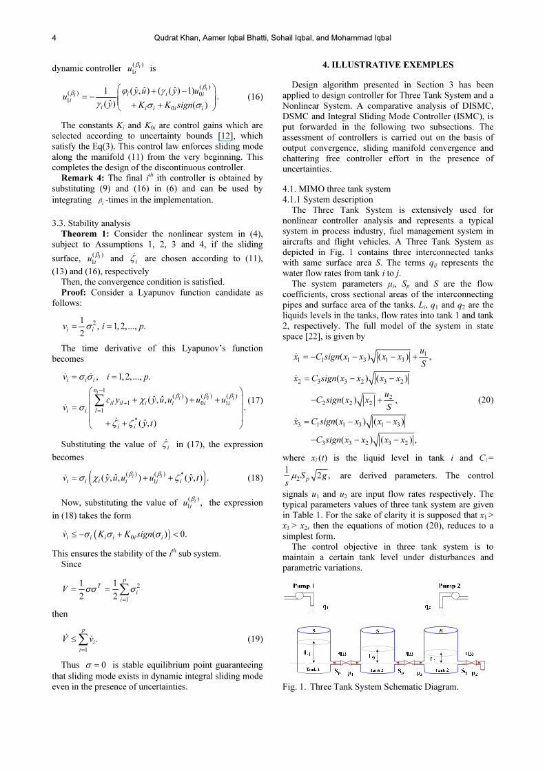
4.1. MIMO three tank system

4.1.1 System description

The Three Tank System is extensively used for

nonlinear controller analysis and represents a typical

system in process industry, fuel management system in

aircrafts and flight vehicles. A Three Tank System as

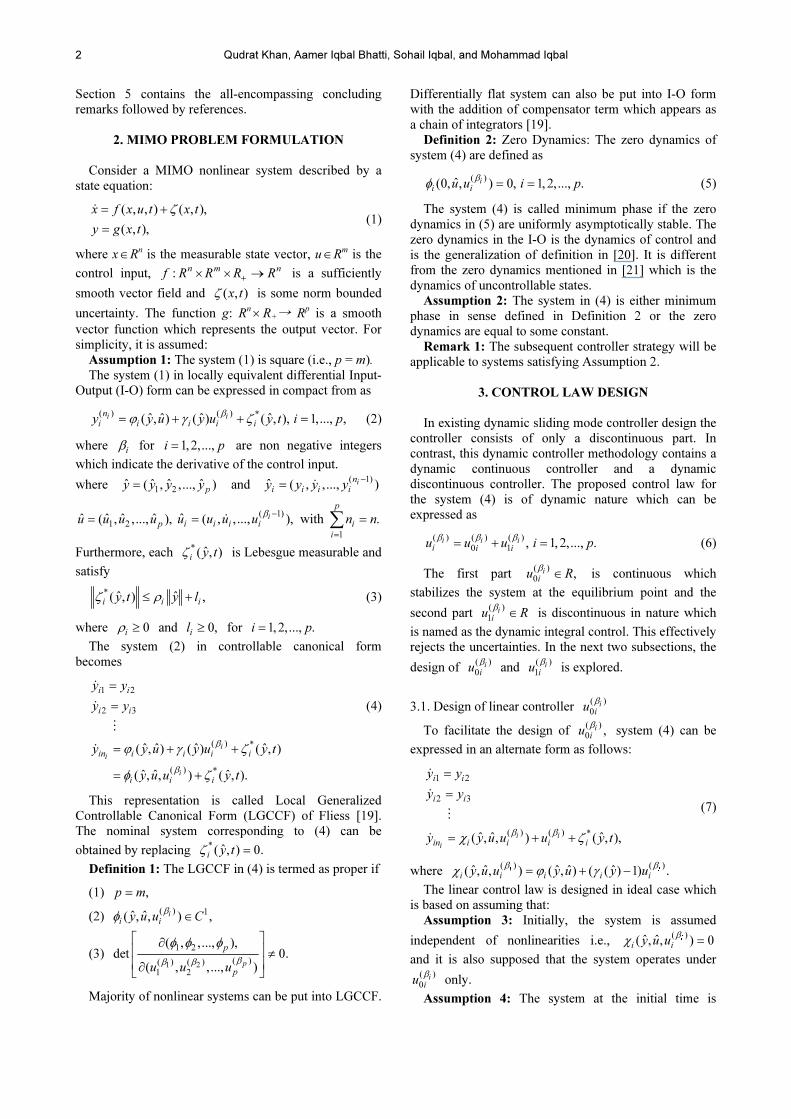
depicted in Fig. 1 contains three interconnected tanks

with same surface area S. The terms qij represents the

water flow rates from tank i to j.

The system parameters µi, Sp and S are the flow

coefficients, cross sectional areas of the interconnecting

pipes and surface area of the tanks. Li, q1 and q2 are the

liquids levels in the tanks, flow rates into tank 1 and tank

2, respectively. The full model of the system in state

space [22], is given by

1

1 1 1 3 1 3

2 3 3 2 3 2

2

2 2 2

3 1 1 3 1 3

3 3 2 3 2

( ) ( ) ,

( ) ( )

( ) ,

( ) ( )

( ) ( ) ,

ux C sign x x x x

S

x C sign x x x x

uC sign x x

S

x C sign x x x x

C sign x x x x

= − − − +

= − −

− +

= − −

− − −

�

�

�

(20)

where xi (t) is the liquid level in tank i and Ci =

2

12 ,

pS g

sµ are derived parameters. The control

signals u1 and u2 are input flow rates respectively. The

typical parameters values of three tank system are given

in Table 1. For the sake of clarity it is supposed that x1 >

x3 > x2, then the equations of motion (20), reduces to a

simplest form.

The control objective in three tank system is to

maintain a certain tank level under disturbances and

parametric variations.

Fig. 1. Three Tank System Schematic Diagram.

Dynamic Integral Sliding Mode for MIMO Uncertain Nonlinear Systems

5

Table 1. Typical parameter values of benchmark TTS.

Parameter Description Nominal Values Units

S Surface area of tanks 0.0154 m2

Sp Surface area of pipes 5x10-5 m2

u1max

u2max Input Flow rates 100 ml/s

yimax

1,2,3i = Maximum level

in tanks 0.62 m

1µ

2µ

3µ

Viscosity or flow

coefficients --

0.5,

0.675

0.5

4.1.2 Controller design

In order to achieve the above task, the proposed

methodology is employed. The outputs of interest are y11

= x1 and y21 = x2. The final expression of the controllers is

as follows:

( )

1 11 11 12 12

1 1

1 3 3 3 2

1 3

1 1 01 1

22

( )

u k y k y

C ux x C x x

Sx x

s K s K sign s

= − −

+ − − + − +

−

− +

�

(21)

and

2 21 21 2 2 02 2( ( .)).u k y s K s K sign s= − − + (22)

4.1.3 Simulation results

The evaluation of the proposed control algorithm is

carried out in the presence of parametric variations and

state dependent uncertainties in three tank system. The

comparative analysis of ISMC, DSMC and DISMC is

executed in the presence of these uncertainties.

Case 1: Output Additive Uncertainty

A state dependent uncertainty

1 2 3( , ) 3 sin( ), 1,2ix t x x x t iζ π= = (23)

is introduced in both the output channels from the very

beginning of the process in simulations. The controllers

gains used in this analysis are defined in Table 2.

The outputs convergence using ISMC, DSMC and the

proposed DISMC are shown in Figs. 2 and 3. It is clear

from both the figures that DISMC quickly steers the

outputs to zero in finite settling time which is

approximately equal to 0.1sec. The response time of

DSMC is 0.8 and 0.1 seconds for the outputs while the

outputs regulation via ISMC oscillates against the origin

with considerable magnitude and high frequency.

Similarly, the convergence of sliding manifolds is shown

in Figs. 4 and 5. It is visible that the convergence of

sliding surface for DSMC and new control law DISMC

are very close to each other. However, the convergence

of DISMC exhibits speedy response. The sliding variable

for ISMC oscillates around the origin.

The control efforts of both controllers are illustrated in

Figs. 6 and 7. One can observe easily that the controller

u1 and u2 via DSMC and proposed control law are chatter

free while that of ISMC has chattering with significant

magnitude. Thus, the proposed controller may evolve as

a better controller as compared to DSMC and ISMC.

Table 2. Parameters of designed controller with additive

uncertainty.

Constants K1 K2 K01 K02 c11 c12 c21 k11 k12 k21

Values 10 0.001 25 1 6.5 31.6 32.60 1

0 0.2 0.4 0.6 0.8 1 1.2 1.4 1.6 1.8 2-0.2

-0.1

0

0.1

0.2

0.3

Time(sec)

Output y1

ISMC

DSMC

DISMC

Fig. 2. y11 trajectories in the presence of uncertainty via

ISMC, DSMC and DISMC.

0 0.2 0.4 0.6 0.8 1 1.2 1.4 1.6 1.8 2-0.04

-0.02

0

0.02

0.04

0.06

0.08

0.1

Time(sec)

Output y2

ISMC

DSMC

DISMC

Fig. 3. y21 trajecotries in the presence of uncertainty via

ISMC, DSMC and DISMC.

0 0.2 0.4 0.6 0.8 1 1.2 1.4 1.6 1.8 2-4

-2

0

2

4

6

8

Time(sec)

Sliding Surface s1

ISMC

DSMC

DISMC

Fig. 4. Sliding Surface s1 convergence for ISMC,

DSMC and DISMC in the presence of

uncertainty.

0 0.2 0.4 0.6 0.8 1 1.2 1.4 1.6 1.8 2-0.8

-0.6

-0.4

-0.2

0

0.2

0.4

0.6

0.8

Time(sec)

Sliding Surface s2

ISMC

DSMC

DISMC

Fig. 5. Sliding Surface s2 convergence for ISMC,

DSMC and DISMC in the presence of

uncertainty.

0 0.05 0.1 0.15 0.2 0.25 0.3 0.35 0.4 0.45 0.5-4

-2

0

2

4

6

8

ISMC

DSMC

DISMC

0 0.05 0.1 0.1

-0.5

0

0.5

ISMC

DSMC

DISMC

Qudrat Khan, Aamer Iqbal Bhatti, Sohail Iqbal, and Mohammad Iqbal

6

0 0.2 0.4 0.6 0.8 1 1.2 1.4 1.6 1.8 2-1.5

-1

-0.5

0

0.5

1

Time(sec)

Control Input u1

ISMC

DSMC

DISMC

Fig. 6. Control Effort u1 via ISMC, DSMC and DISMC

in the presence of uncertainty.

0 0.2 0.4 0.6 0.8 1 1.2 1.4 1.6 1.8 2-0.4

-0.3

-0.2

-0.1

0

0.1

0.2

0.3

Time(sec)

Control Input u2

ISMC

DSMC

DISMC

Fig. 7. Control Effort u2 via ISMC, DSMC and DISMC

in the presence of uncertainty.

Case 2: Parametric Variations

This experiment involves the evaluation of the

proposed controller under parametric variations in the

Three Tank System. This system has four parameters s,

c1, c2 and c3 with their nominal values 0.0154, 0.0072,

0.0097 and 0.0072, respectively. These parameters are

varied with 30% increase in each. These varitions are

initiated in the system in steady state. The controller

gains are give in Table 3.

The convergence of the outputs y11 and y21 is displayed

in Figs. 8 and 9. This ensures the quick and oscillation

free convergence of the outputs to the origin via DISMC.

On the other hand, it is obvious from these figures that

outputs convergence of DSMC is not only slower than

that of DISMC but is also oscillatory in behavior. In

addition, the output of ISMC has fast convergence but

shows oscillatory pattern with high frequency and

considerable magnitude as illustrated in the zoomed

views in Figs. 8 and 9.

0 5 10 15 20 25 30-0.05

0

0.05

0.1

Time(sec)

Output y2

ISMC

DSMC

DISMC

Fig. 9. y21 trajecotries in the presence of parametric

variation via ISMC, DSMC and DISMC.

0 5 10 15 20 25 30-0.4

-0.3

-0.2

-0.1

0

0.1

0.2

0.3

Time(sec)

Control Input u1

ISMC

DSMC

DISMC

Fig. 10. Control Effort u1 via ISMC, DSMC and DISMC

in the presence of parametric variation.

0 5 10 15 20 25 30-0.15

-0.1

-0.05

0

0.05

0.1

Time(sec)

Control Input u2

ISMC

DSMC

DISMC

Fig. 11. Control Effort u2 via ISMC, DSMC and DISMC

in the presence of parametric variation.

Figs. 10 and 11, confirm the chattering free nature of

DISMC. It is obvious that ISMC controller experiences

chattering phenomena. Similarly, the DSMC controller

exhibits oscillation and a significant peak appears when

the variations are introduced. In this regards, the

proposed controller may be superior to the other two

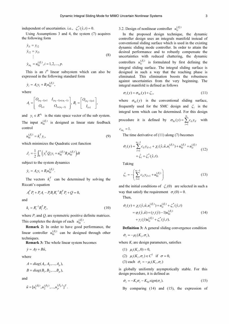
controllers. Same analysis can be seen in Figs. 12 and 13.

The convergence of sliding manifolds is displayed over

there.

0 5 10 15 20 25 30-2

0

2

4

6

8

Time(sec)

Sliding Surface s1

ISMC

DSMC

DISMC

Fig. 12. Sliding Surface s1 convergence for ISMC,

DSMC and DISMC in the presence of

parametric variations.

0 0.05 0.1 0.15 0.2 0.25 0.3 0.35 0.4 0.45 0.5-1.5

-1

-0.5

0

0.5

1

ISMC

DSMC

DISMC

0 0.02 0.04 0.06 0.08 0.1 0.12 0.14 0.16 0.18 0.2.4

.2

0

.2

.4

ISMC

DSMC

DISMC

Table 3. Parameter values for designed controller with

parametric variations.

Constants K1 K2 K01 K02 c11 c12 c21 k11 k12 k21

Values 3 0.001 25 1 3 31.6 32.6 1

0 5 10 15 20 25 30-0.1

-0.05

0

0.05

0.1

0.15

0.2

0.25

0.3

Time(sec)

Output y1

ISMC

DSMC

DISMC

Fig. 8. y11 trajecotries in the presence of parametric

variation via ISMC, DSMC and DISMC.

10 15 20 25

-4

-2

0

x 10-5

Time(sec)

Output y1

15 20 25 30

-3

-2

-1

0

x 10-4

ISMC

DSMC

DISMC

0 5 10 15 20 25 30-5

0

5x 10

-4

Time(sec)

Output y2

19 20 21 22 23 24 25 26 27 28 29 30

-5

0

5

10x 10

-5

ISMC

DSMC

DISMC

15 20 25 300

2

4

6

8

10x 10

-5

ISMC

DSMC

DISMC

Dynamic Integral Sliding Mode for MIMO Uncertain Nonlinear Systems

7

0 5 10 15 20 25 30-0.1

-0.05

0

0.05

0.1

0.15

0.2

0.25

0.3

Time(Sec)

Sliding Surface S2

ISMC

DSMC

DISMC

Fig. 13. Sliding Surface s2 convergence for ISMC,

DSMC and DISMC in the presence of

parametric variations.

The aforementioned comparative analysis confirms the

robust and chatters free nature of DISMC along with

enhanced performance.

4.2. MIMO non linear system

4.2.1 System description

Consider another MIMO nonlinear system represented

by the following state space equations [33].

1 2

2

2 1 3 1 4 3 1

3 4

3

4 1 3 1 2

,

cos ,

,

cos ,

x x

x qx x x x x u

x x

x wx x x u

=

= + + +

=

= − +

�

�

�

�

(24)

where x1, x2, x3, x4 are states and u1 and u2 are the inputs

to the nonlinear system. q and w are the parameters with

their nominal values 3 and 1, respectively. In this study,

the objective is to regulate the outputs from some initial

position to the desired equilibrium point (origin). The

outputs of interest are y11 = x2 and y21 = x4. The relative

degree of the system with respect to both the output

functions is 1.

4.2.2 Controller design

For the controller design, again following the scheme

of Section 3, the expressions of the discontinuous

controllers becomes

0 1 1 2 2.

i i i i iu k y k y= − −� (25)

The gains kij are considered in Table 4.

11 2 3 4 2 4 3

3 2

1 1 3 1 2 3 1 4 3

1 1 01 1

2 cos

( cos )cos sin

( ).

u qx x x x x x

x wx x x u x x x x

K s K sign s

= − − −

− − + +

− −

�

2

12 1 2 4 1 2 3 1

2 2 02 2

( cos sin )

( ).

u wx x x x x x x

K s K sign s

= − − −

− −

�

Therefore, the final form for the control laws can be

obtained by using

0 1.

i i iu u u= +� � �

This completes the controller design for the prescribed

system. The characteristic of the controller are discussed

in the following simulation results.

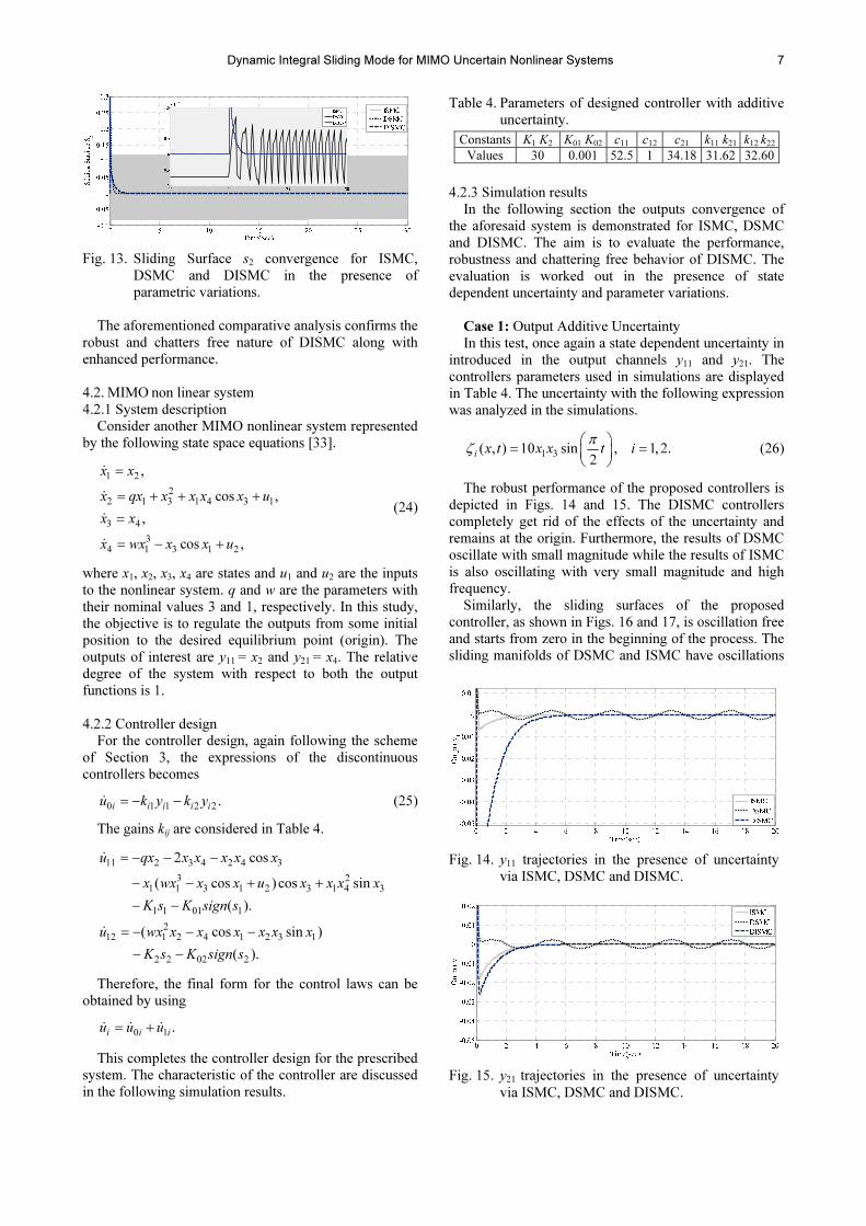
Table 4. Parameters of designed controller with additive

uncertainty.

Constants K1 K2 K01 K02 c11 c12 c21 k11 k21 k12 k22

Values 30 0.001 52.5 1 34.18 31.62 32.60

4.2.3 Simulation results

In the following section the outputs convergence of

the aforesaid system is demonstrated for ISMC, DSMC

and DISMC. The aim is to evaluate the performance,

robustness and chattering free behavior of DISMC. The

evaluation is worked out in the presence of state

dependent uncertainty and parameter variations.

Case 1: Output Additive Uncertainty

In this test, once again a state dependent uncertainty in

introduced in the output channels y11 and y21. The

controllers parameters used in simulations are displayed

in Table 4. The uncertainty with the following expression

was analyzed in the simulations.

1 3( , ) 10 sin , 1,2.

2ix t x x t i

πζ

= =

(26)

The robust performance of the proposed controllers is

depicted in Figs. 14 and 15. The DISMC controllers

completely get rid of the effects of the uncertainty and

remains at the origin. Furthermore, the results of DSMC

oscillate with small magnitude while the results of ISMC

is also oscillating with very small magnitude and high

frequency.

Similarly, the sliding surfaces of the proposed

controller, as shown in Figs. 16 and 17, is oscillation free

and starts from zero in the beginning of the process. The

sliding manifolds of DSMC and ISMC have oscillations

15 20 25 30-1

-0.5

0

0.5

1

1.5x 10

-4

ISMC

DSMC

DISMC

0 2 4 6 8 10 12 14 16 18 20-0.05

-0.04

-0.03

-0.02

-0.01

0

0.01

Time(sec)

Output y1

ISMC

DSMC

DISMC

Fig. 14. y11 trajectories in the presence of uncertainty

via ISMC, DSMC and DISMC.

0 2 4 6 8 10 12 14 16 18 20-0.05

-0.04

-0.03

-0.02

-0.01

0

0.01

0.02

Time(sec)

Output y2

ISMC

DSMC

DISMC

Fig. 15. y21 trajectories in the presence of uncertainty

via ISMC, DSMC and DISMC.

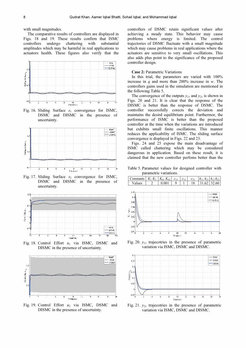
Qudrat Khan, Aamer Iqbal Bhatti, Sohail Iqbal, and Mohammad Iqbal

8

with small magnitudes.

The comparative results of controllers are displayed in

Figs. 18 and 19. These results confirm that ISMC

controllers undergo chattering with substantial

amplitudes which may be harmful in real applications to

actuators health. These figures also verify that the

controllers of DSMC retain significant values after

achieving a steady state. This behavior may cause

problems where energy is limited. The control

trajectories of DSMC fluctuate with a small magnitude

which may cause problems in real applications where the

actuators are sensitive to very small oscillations. This

also adds plus point to the significance of the proposed

controller design.

Case 2: Parametric Variations

In this trial, the parameters are varied with 100%

increase in q and more than 200% increase in w. The

controllers gains used in the simulation are mentioned in

the following Table 5.

The convergence of the outputs y11 and y21 is shown in

Figs. 20 and 21. It is clear that the response of the

DISMC is better than the response of DSMC. The

controller successfully corects the deviation and

maintains the desird equilibrium point. Furthermor, the

performance of ISMC is better than the proposed

controller at the time when the variations are introduced

but exhibits small finite oscillations. This manner

reduces the applicability of ISMC. The sliding surface

convergence is displayed in Figs. 22 and 23.

Figs. 24 and 25 expose the main disadvantage of

ISMC called chattering which may be considered

dangerous in application. Based on these result, it is

claimed that the new controller perfoms better than the

Table 5. Parameter values for designed controller with

parametric variations.

Constants K1 K2 K01 K02 c11 c12 c21 k11 k21 k12 k22

Values 2 0.001 9 1 18 31.62 32.60

0 2 4 6 8 10 12 14 16 18 20-0.04

-0.02

0

0.02

0.04

0.06

0.08

0.1

0.12

Time(sec)

Output y1

ISMC

DSMC

DISMC

Fig. 20. y11 trajecotries in the presence of parametric

variation via ISMC, DSMC and DISMC.

0 2 4 6 8 10 12 14 16 18 20-0.05

0

0.05

0.1

0.15

0.2

0.25

0.3

Time(sec)

Ou

tpu

t y

2

ISMC

DSMC

DISMC

Fig. 21. y21 trajecotries in the presence of parametric

variation via ISMC, DSMC and DISMC.

0 2 4 6 8 10 12 14 16 18 20-0.5

0

0.5

1

1.5

2

Time(Sec)

Sliding Surface s1

ISMC

DSMC

DISMC

Fig. 16. Sliding Surface s1 convergence for ISMC,

DSMC and DISMC in the presence of

uncertainty.

0 2 4 6 8 10 12 14 16 18 20-0.5

0

0.5

1

1.5

2

Time(sec)

Sliding Surface s2

ISMC

DSMC

DISMC

Fig. 17. Sliding Surface s2 convergence for ISMC,

DSMC and DISMC in the presence of

uncertainty.

0 2 4 6 8 10 12 14 16 18 20-3

-2.5

-2

-1.5

-1

-0.5

0

0.5

Time(sec)

Control Input u1

ISMC

DSMC

DISMC

Fig. 18. Control Effort u1 via ISMC, DSMC and

DISMC in the presence of uncertainty.

0 2 4 6 8 10 12 14 16 18 20-1

-0.5

0

0.5

1

Time(sec)

Control Input u2

ISMC

DSMC

DISMC

Fig. 19. Control Effort u2 via ISMC, DSMC and

DISMC in the presence of uncertainty.

Dynamic Integral Sliding Mode for MIMO Uncertain Nonlinear Systems

9

other two controllers.

Table 6 contains all the attributes utilized to evaluate

the proposed DISMC. Based on the results enumerated in

Table 6 and shown above figures, it can be claimed that

proposed DISMC outshines DSMC and ISMC control in

maximum aspects.

Table 6. Comparative analysis of ISMC, DSMC and

DISMC.

ATTRIBUTES ISMC DSMC DISMC

Robustness

Rejects the

uncertainties

with high

frequency

oscillations

Rejects the

uncertainties

but with slight

deviation from

the origin

Effectively

rejects the

uncertainties

with very small

deviation

Settling

Time Small

Comparatively

Large Small

Oscillations

High

Frequency

Oscillations

with significant

magnitude.

Oscillations

exists in some

cases

No Oscillations

Regulation

Control

To the vicinity

of the origin

To the vicinity

of the origin

Exactly to the

Origin

Chattering

Analysis

Severe

chattering.

No chattering

but oscillatory

response

No chattering

&

No oscillations

Sliding

Surface

Convergence

Chattering

exists with

considerable

magnitude.

Converges to

origin with

slight chattering

in some cases

Converges to

(origin),

No chattering

Control EffortHigh control

efforts.

High Controller

efforts

Low control

efforts

Computational

Complication

Low

computation

complexities

Low

computation

complexities

Comparatively

high

computation

complexities

5. CONCLUSIONS

In this work, a novel dynamic integral sliding mode

approach is proposed for a class of MIMO uncertain

nonlinear systems. This design methodology synthesizes

DSMC and ISMC technique into the so-called Dynamic

Integral Sliding Mode. This provides dynamic controller

which enforces sliding mode along the integral manifold

from the beginning of the process. Consequently, sliding

mode without reaching phase is established. This

elimination enhances robustness of the proposed

controller against uncertainties. The robustness is also

inherited from DSMC. The control law designed via the

proposed strategy comprises of two terms. The first term

improved the performance of the control law and the

second term performed for improving robustness. In

addition, the proposed control law establishes sliding

mode with reduced chattering phenomena. Thus, it is

claimed that the new designed technique captured the

good features of ISMC and DSMC. Based on the

simulation results it can also be claimed that the

proposed DISMC outshines DSMC and ISMC control in

maximum aspects.

REFERENCES

[1] C. Edwards and S. K. Spurgeon, Sliding Mode Con-

trol: Theory and Applications, Taylor and Francis,

London, 1998.

[2] V. I. Utkin, Sliding Mode Control in Electrome-

chanical Systems, Taylor and Francis, 1999.

[3] S. H. Zak and S. Hui, “On variable structure output

0 2 4 6 8 10 12 14 16 18 20-0.5

0

0.5

1

1.5

2

2.5

Time(sec)

Sliding Surface s1

ISMC

DSMC

DISMC

Fig. 22. Sliding Surface s1 convergence for ISMC,

DSMC and DISMC in the presence of

uncertainty.

0 2 4 6 8 10 12 14 16 18 20-1

0

1

2

3

4

5

Time(sec)

S

liding S

urface s2

ISMC

DSMC

DISMC

Fig. 23. Sliding Surface s2 convergence for ISMC,

DSMC and DISMC in the presence of

uncertainty.

0 2 4 6 8 10 12 14 16 18 20-1.4

-1.2

-1

-0.8

-0.6

-0.4

-0.2

0

Time(sec)

C

ontrol Input u1

ISMC

DSMC

DISMC

Fig. 24. Control Effort u1 via ISMC, DSMC and

DISMC in the presence of parametric variation.

0 2 4 6 8 10 12 14 16 18 20-0.5

-0.4

-0.3

-0.2

-0.1

0

0.1

0.2

0.3

Time(sec)

Control Input u2

ISMC

DSMC

DISMC

Fig. 25. Control Effort u2 via ISMC, DSMC and

DISMC in the presence of parametric variation.

Qudrat Khan, Aamer Iqbal Bhatti, Sohail Iqbal, and Mohammad Iqbal

10

feedback controllers for uncertain dynamic sys-

tems,” IEEE Trans. on Automatic Control, vol. 38,

no. 10, pp. 1509-1512, 1993.

[4] C. Edwards and S. K. Spurgeon, “Sliding mode

stabilization of uncertain systems using only output

information,” International Journal of Control, vol.

62, no. 5, pp. 1129-1144, 1995.

[5] K. K. Shyu, Y. W. Tasi, and C. K. Lai, “A dynamic

output feedback controller for mismatch uncertain

variable structure systems,” Automatica, vol. 37, no.

5, pp. 775-779, 2001.

[6] J. M. Andrade-Da Silva, C. Edwards, and S. K.

Spurgeon, “Sliding-mode output-feedback control

based on LMIs for plants with mismatched uncer-

tainties,” IEEE Trans. on Ind. Electronics, vol. 56,

no. 9, pp. 3675-3683, 2009.

[7] J.-L. Chang, “Dynamic output integral sliding-

mode control with disturbance attenuation,” IEEE

Trans. on Automatic Control, vol. 54, no. 11, pp.

2653-2658, 2009.

[8] W. J. Cao and J.-X. Xu, “Nonlinear integral-type

sliding surface for both matched and unmatched

uncertain systems,” IEEE Trans. on Automatic

Control, vol. 49, no. 8, pp. 1355-1360, 2004.

[9] Y.-J. Cheon, “Sliding mode control of spacecraft

with actuator dynamics,” Trans. on Control Auto-

mation, and Systems Engineering, vol. 4, no. 2, pp.

169-175, 2002.

[10] H. Sira-Ramirez, “A dynamical variable structure

control strategy in asymptotic output tracking prob-

lems,” IEEE Trans. on Automatic Control, vol. 38,

no. 4, pp. 615-620, 1993.

[11] G. Bartolini, A. Ferrara, and E. Usai, “Chattering

avoidance by second order sliding mode control,”

IEEE Trans. on Automatic Control, vol. 43, no. 2,

pp. 241-246, 1998.

[12] L. Fridman and A. Levant, Higher order sliding

modes, In W. Perruquetti, J. P. Barbot, eds., Sliding

mode Control in Engineering, Marcel Dekker, Inc.,

53-101, 2002.

[13] A. Levant, “Sliding order and sliding accuracy in

sliding mode control,” International Journal of

Control, vol. 58, no. 6, pp. 1247-1267, 1993.

[14] T. Floquet, J. P. Barbot, and W. Perruquetti, “High-

er order sliding mode stabilization for a class of

nonholonomic perturbed systems,” Automatica, vol.

39, no. 6, pp. 1077-1083, 2003.

[15] S. Laghrouche, F. Plestan, and A. Alain Gluminea,

“Higher order sliding mode control based on

integral sliding mode,” Automatica, vol. 43, no. 3,

pp. 531-537, 2007.

[16] A. Levant and L. Alelishvili, “Integral high-order

sliding modes,” IEEE Trans. on Automatic Control,

vol. 52, no. 7, pp. 1278-1282, 2007.

[17] K. Furuta, and Y. Pan, “Variable structure control

with sliding sector,” Automatica, vol. 36, pp. 211-

228, 2000.

[18] H. Sira-Ramirez, “On the dynamical sliding mode

control of nonlinear systems,” International Jour-

nal Control, vol. 57, no. 5, pp. 1039-1061, 1993.

[19] M. Fliess, “Generalized controller canonical form

for linear systems and nonlinear dynamics,” IEEE

Trans. on Autmaictic control, vol. 35,no. 9, pp. 994-

1001, 1990.

[20] M. Fliess, Nonlinear control theory and differential

algebra. In C. Byrnes, A. Kurzhanski, (Eds), Mod-

eling and Adaptive Control. vol. 105 of Lecture

notes in Control and Information Sciences, Sprin-

ger-Verlag, New York, pp. 134-145, 1988.

[21] A. Isidori, Nonlinear Control Systems, 3rd Ed.,

Springer-Verlag, 1995.

[22] M. Iqbal, A. I. Bhatti, S. Iqbal, and Q. Khan, “Ro-

bust parameter estimation of nonlinear systems us-

ing sliding mode technique,” IEEE Trans. on Ind.

Electronics, published online: March, 2010.

Qudrat Khan is a postgraduate student

with the Department of Electronic Engi-

neering Mohammad Ali Jinnah Universi-

ty Islamabad, Pakistan. His professional

interests are observer design and parame-

ter estimation, theory of sliding mode

control and its application and analytical

dynamics.

Aamer Iqbal Bhatti got his Bachelor’s

degree in Electrical Engineering from

UET Lahore in 1993; Masters in Control

Systems from Imperial College of

Science, Technology & Medicine, Lon-

don, in 1994. He did his Ph.D. and post-

doctorial research in Control Engineering

in 1998, 1999 from Leicester University

UK. Currently, he is a Professor of DSP

and Control Systems. His research interests are Sliding Mode

Applications and Radar Signal Processing and have published

more than 68 refereed research papers.

Sohail Iqbal is doing his Ph.D. from

Mohammad Ali Jinnah University, Isla-

mabad. Currently, he is with university of

Leicester, UK as Research Fellow. His

research interests are Control Theory &

Robotics Systems emphasizing on High-

er Order Sliding Mode Theory and Paral-

lel Robotic Manipulators.

Mohammad Iqbal is a Ph.D. candidate

at Center for Advanced Studies in Engi-

neering (CASE), Islamabad. He is the

first author and co-author of more than

16 refereed international publications.

His research interests are Controls &

DSP applications emphasizing Fault Di-

agnosis of uncertain Nonlinear Dynamic

Systems.