Implicit methods of solution to integral formulations in boundary element method based nearfield...

Implicit methods of solution to integral formulations inboundary element method based nearfield acoustic holography

Nicolas Valdiviaa) and Earl G. WilliamsCode 7130, Naval Research Laboratory, Washington, DC 20375

~Received 8 September 2003; revised 17 May 2004; accepted 10 June 2004!

Two integral equation methods are considered which can be inverted to provide the surface velocityand/or pressure given a measurement of the pressure on an imaginary surface in the nearfield of avibrating or scattering body. This problem is central to nearfield acoustical holography~NAH!. Theintegral equations are discretized using boundary element methods~BEMs!. The integral equationmethods considered are~1! an indirect formulation method based on the single layer integralequation and~2! a direct formulation method based on a system of equations derived from theHelmholtz–Kirchhoff integral equation. The formation of integral equations from the mentionedmethods will not involve the explicit inversion of matrices, but instead will require this inversion tobe done implicitly. Since these methods back-track the sound field from the measurement surface tothe surface of the source/vibrator they are ill-posed in nature and Tikhonov regularization are usedto stabilize the reconstruction. Problems are noted with the use of higher order shape functions inthe BEM discretization which are detrimental to the inversion, and it is shown that the breakdownof the method at the interior resonance frequencies can be mitigated successfully. These twoapproaches are compared with the conventional direct method using measured experimental datafrom a point-driven rectangular plate. ©2004 Acoustical Society of America.@DOI: 10.1121/1.1777854#

PACS numbers: 43.40.Sk, 43.20.Rz, 43.40.Yq@MO# Pages: 1559–1572

uehonantio. Ifr

trsmso

’snge

e

n

it

aybl

is

twoing

dininto

thethetorr-

rmu-ic

hes,raln thesure

thees

, inat-canonich

I. INTRODUCTION

The reconstruction of the acoustic field~pressure, nor-mal velocity, and intensity! plays an important role in theearly stage of effective noise control. A powerful techniqused for this reconstruction is called nearfield acousticallography~NAH!.1 NAH has had a tremendous success alyzing sources with geometries which conform closely to oof the separable geometries of the acoustic wave equafor example, planar, cylindrical, and spherical geometriesthese analyses, the pressure field radiated or scatteredan object is measured on an imaginary surface outside~forexterior problems! or inside ~for interior problems! thesource. NAH uses this pressure hologram to reconstructacoustic field on the body of the source, an ill-posed inveproblem. The solution of the inverse problem in these geoetries relies on the expansion of the pressure field in terma complete set of eigenfunctions along with a knowledgethe analytical form of the Neumann or Dirichlet Greenfunction. The reconstructions are very efficient, requirionly fractions of a second of computation time per frquency. Sources with boundaries which vary appreciablyshape from one of these separable geometries can btacked using boundary element methods~BEMs! whichyields a numerical form of the appropriate Green’s functioalong with the singular value decomposition~SVD! whichprovides orthonormal eigenfunctions for the geometry. Wthese eigenfunctions, the methodology of the inversionidentical to that used for the separable geometry. One phowever, for the expanded versatility with a considera

a!Electronic mail: [email protected]

J. Acoust. Soc. Am. 116 (3), September 2004 0001-4966/2004/116(3)/1

--

en;nom

hee-

off

-inat-

,

hiss,

e

increase in computation time. This generalization of NAHcalled IBEM—inverse boundary element method.

Inverse boundary element methods are broken intoclasses of formulations: the direct formulations which sprfrom the Helmholtz–Kirchhoff integral equation~HIE! andthe indirect formulations which manipulate the HIE ansolve for a fictitious source distribution. The first papersIBEM-NAH used the direct formulation and appeared1988.2–4An extensive comparison of different approachesdirect formulation IBEM was given in 1992.5 Complicatedunderwater axisymmetric vibrators were studied usingdirect formulation and conformal measurement sets inearly 1990s.6–8 Precise and automated approachesregularization9,10 of the inversion first appeared in 1996 fothe direct formulation,11 and general discussions of regulaization useful for NAH and IBEM-NAH appeared later.12–16

Other researches of note have appeared on the direct folation IBEM,17–19 and on methods using spherical harmonexpansions in an effort to improve accuracy.20

The second popular approach to NAH using IBEM is tindirect formulation in which fictitious source distributionwhich are the kernels of single and/or double layer integrepresentations, are used as an intermediate step betweemeasured pressure and the reconstructed velocity or presfields.21–24 We call these methods indirectimplicit formula-tions since the creation of the transfer function betweensurface velocity~or pressure! and the measured pressure donot require a matrix inversion. The last two cited papersfact, make use of this property and thus are particularlytractive for very large matrices since iterative approachesbe used, although formulation of effective regularizatimethods is a major issue here. A larger body of work, wh

1559559/14/$20.00 © 2004 Acoustical Society of America

ine

rae-tia

ichu

onh

mlaboWul

-d

e

-

ns

ilureth

-

te-

ite

n-een

ors

in

onstoer-

ofs

ri-ra-

areexplicit in nature since they require computation andversion of full matrices, use a variational principle in thindirect formulation and start with the double layer integrepresentation.25–31This variation approach is sometimes rferred to as IVBEM~indirect variational boundary elemenmethod! and it is being used in several major commerccomputer codes.

We present in this paper two implicit approaches whhave not been investigated in the literature, a direct formlation based on the solution of a system of integral equatiand an indirect formulation based on the single layer. Tlatter is attractive for its theoretical and computational siplicity. It does not require computation of a hyper-singukernel needed for the variational approaches discussed aand does not require any intermediate matrix inversions.compare these approaches to the traditional direct formtion to illustrate their accuracy.

II. BOUNDARY INTEGRAL REPRESENTATION

Let D be a domain inR3, interior to the boundary surfaceG where we assume thatG is allowed to have edges ancorners. Similarly we will denote asD1 the region outside ofD that shares the same boundaryG. For a time-harmonic(e2 ivt) disturbance of frequencyv the sound pressurep sat-isfies the homogeneous Helmholtz equation inD ~or D1),

Dp1k2p50, ~1!

wherek5v/c is the wave number andc is the constant forthe speed of sound. A solutionp that satisfies Eq.~1! in D1

also needs to satisfy the Sommerfeld radiation condition~seeRef. 32!.

In this work we will consider exterior NAH, where thacoustical sensors are placed on a surfaceG0 outside thedomainD. These are used to measure the pressurep and thefundamental problem is to recover the acoustic field~pres-sure, normal velocity, and normal intensity! on G. The solu-tion for NAH by the direct formulation is based on theHelmholtz–Kirchhoff integral equation ~HIE!, for x5(x1 ,x2 ,x3)PD1

p~x!5~Dp!~x!2 ivr~Sv !~x!, ~2!

which is a solution to Eq.~1! ~see Ref. 32!. In Eq. ~2! we usean integral operator notation similar to33,32

~Sw!~x!ªEGF~x,y!w~y!dS~y!, xPR3, ~3!

~Dw!~x!ªEG

]F~x,y!

]n~y!w~y!dS~y!, xPD1, ~4!

whereF is the free space Green’s functionto the Helmholtzequation

F~x,y!5exp~ ikux2yu!

4pux2yu. ~5!

In Eq. ~2!, r is the mean fluid density and in Eq.~4!, n is theunit interior normal toG. As described in Ref. 33, Theorem2.13, there is a jump relation in Eq.~4! whenxPG,

1560 J. Acoust. Soc. Am., Vol. 116, No. 3, September 2004 Va

-

l

l

-se-rveea-

~Dw!1~x!ªEG

]F~x,y!

]n~y!w~y!dS~y!1V~x!w~x!, ~6!

whereV~x! is the solid angle coefficient given by the integral formula

V~x!52EG

]

]n~y! S 1

4pux2yu DdS~y!, xPG. ~7!

V~x! will be 12 for all xPG, whenG is a smooth surface.

The indirect formulationsare based on representatioto the solution of Eq.~1! like the single source~or singlelayer! representation21–24

p~x!5~Sw!~x!, xPR3, ~8!

wherew is the density function, and the double source~ordouble layer! representation25–31

p~x!5~Dw!~x!, xPD1. ~9!

The double source representation is used to avoid the faof HIE whenD is a thin shape body or a regular body wiappendages.

The traditional approach for solving NAH~both for di-rect and indirect formulations! is based on the integral equations

p~x!5EGG~x,y!p~y!dS~y!, xPG0 , ~10!

and

p~x!5EGG8~x,y!v~y!dS~y!, xPG0 , ~11!

where the functionsG andG8 are respectively theDirichletGreen’s functionandNeumann Green’s functionfor Eq. ~1!.These integral equations are similar to the Rayleigh’s ingral formulas for planar NAH~see Ref. 1!, since an explicitrelationship betweenp on the measurement surfaceG0 andp,v on G is given. In general, the knowledge of an explicformula for these functions will be helpful, but can only bfound for some restricted geometries~see Refs. 34–36!. Inthe acoustical literature, to overcome this difficulty for geeral surfaces, effective numerical approximations have bapplied. The common practice~see Refs. 5, 11, 14, and 29!will be to combine the direct formulation in Eq.~2! with Eq.~6! to produce a numerical approximation of the operatgiven by Eqs.~10! and ~11!. We will refer to this particularapproach as thedirect-explicit~DE! approach, and provide amore detailed discussion in the next section. SimilarlyRefs. 25–31 the indirect formulation in Eq.~9! is used witha variational approach to create a numerical approximatiof Eqs. ~10! and ~11!. The variational approach is usedovercome some of the difficulties related to the hypsingular integral equation created by the normal derivativethe integral operator in Eq.~9!. This approach is known athe inverse variational boundary elements~IVBEMs!. Wewill not discuss IVBEM any further, since previous compasons with the DE approach are available in the cited liteture.

ldivia and Williams: Implicit methods for nearfield acoustic holography

thp

nharhe

nec4

or

uheitse

nse

u

o

e

-

atri-

r-es,ap-

nit

As explained above, the traditional approach uses eidirect or indirect formulations to produce a numerical aproximation of the transfer functions in Eqs.~10! and ~11!.There are special approaches that will not require thesemerical approximations of the transfer functions, and for treason will be calledimplicit approaches. In this work ouinterest will focus on two particular implicit approaches: tdirect-implicit ~DM! approach and theindirect-implicit ~IM !approach. The DM approach uses the direct formulationEq. ~2! combined with Eq.~6! to construct theHelmholtz–Kirchhoff system~suggested in Ref. 37!. The solution to thissystem will provide the reconstruction of both pressure anormal velocity. The explicit formula for this system will bgiven in Sec. III. Finally, the IM approach uses the indireformulation in Eq.~8! ~as suggested in Refs. 23, 22, and 2!to solve

p~x!5~Sw!~x!, xPG0 , ~12!

for the densityw. Then usew to obtain

v~x!51

ivr~Kw!1~x!, xPG, ~13!

where K is the normal derivative of the integral operat(Sw)(x) in Eq. ~3!, whenxPG. The formula of this normalderivative is given in Ref. 33, Theorem 2.19,

~Kw!1~x!ªEG

]F~x,y!

]n~x!w~y!dS~y!2V~x!w~x!. ~14!

The pressure overG will be obtained using the densityw onthe integral Eq.~8! evaluated atxPG.

III. NUMERICAL IMPLEMENTATION

As exposed in the previous sections the NAH techniqwill be reduced to the solution of integral equations. Tnumerical solution of an integral equation is based ondiscretization, which is a reduction into a linear matrix sytem where numerical methods can be applied. Boundaryement methods~BEMs! will be used as the discretizatiomethod in this work since they have been successfully uin the area of acoustic radiation and scattering~see Refs. 5,17, 11, 38, 39, and 28! for three-dimensional surfaces.

A. BEM discretization of integral equations

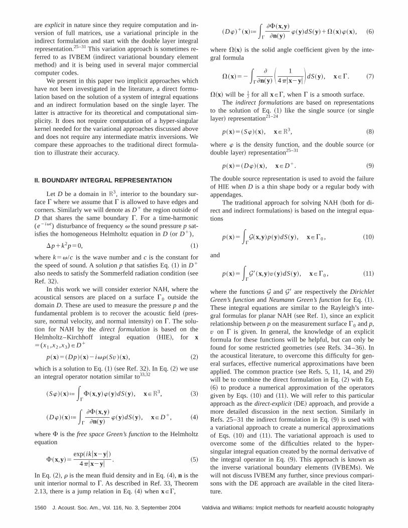
The boundary elements used for approximating the sface integral are schematically shown in Fig. 1.Nv triangularelements are used in this study for the constructionmeshes. The global Cartesian coordinatesy on any point ofan element~denoted asD j , j 51,...,Nv) are assumed to brelated to the nodesym , m51,...,q, by

y~j!5 (m51

q

Nm~j!ym , ~15!

in which j5(j1 ,j2), q53 andNm(j) are linear shape functions defined as

N1~j1 ,j2!5u, N2~j1 ,j2!5j2 ,~16!

N3~j1 ,j2!5j1 , u512j12j2 ,

J. Acoust. Soc. Am., Vol. 116, No. 3, September 2004 Valdivia a

er-

u-t

in

d

t

e

s-l-

d

r-

f

or quadratic shape functions withq56

N1~j1 ,j2!5u~2u21!, N2~j1 ,j2!5j2~2j221!,

N3~j1 ,j2!5j1~2j121!, N4~j1 ,j2!54j2u, ~17!

N5~j1 ,j2!54j1j2 , N6~j1 ,j2!54j1u.

Equation~15! is an isoparametric transformation in whichsurface element is mapped into a plane equilateral unitangle ~as in the lower part of Fig. 1!. Next, the boundaryvariablew given in Eqs.~3!, ~4!, ~6!, and~14! will be repre-sented on each elementj according to

w~j!5 (m51

q

Nm~j!w~m, j ! , ~18!

wherew (m, j ) are the values ofw at nodem of the elementj.For xiPD1, we have that for the integral in Eqs.~3! and~4!

~Sw!~xi !'(j 51

Nv

(m51

q

S~m, j !i w~m, j ! , ~19!

~Dw!~xi !'(j 51

Nv

(m51

q

D ~m, j !i w~m, j ! , ~20!

where

S~m, j !i 5E

0

1E0

12j2F~xi ,y~j1 ,j2!!Nm~j1 ,j2!

3J~j1 ,j2!dj1 dj2 , ~21!

D ~m, j !i 5E

0

1E0

12j2 ]F~xi ,y~j1 ,j2!!

]n~y~j1 ,j2!!Nm~j1 ,j2!

3J~j1 ,j2!dj1 dj2 , ~22!

in which J(j1 ,j2) is the Jacobian of the coordinate transfomation. This Jacobian is known exactly for some surfachowever for general surfaces it is more convenient to

FIG. 1. Boundary elements used in iso-parametric transformation.~a! Linearelements.~b! Quadratic elements. The lower part of the figure shows the utriangles.

1561nd Williams: Implicit methods for nearfield acoustic holography

.-a

ou

r-3.

if

.

er

-

-

wio

g

.

ea-it

ecialred.eri-

ar

dre-

c

proximate it numerically using Eq.~15! as suggested in Ref40. IntegralsS(m, j )

i , D (m, j )i are approximated numerically us

ing the adaptive integration scheme given in Ref. 41, Ch9, with the formula (T2 :5.1) from Ref. 42, Chap. 8.

For xiPG we have that the integral on Eq.~3! will beapproximated as in Eq.~19!, and the integrals on Eqs.~6!and ~14! will be

~Dw!1~xi !'(j 51

Nv

(m51

q

D ~m, j !i w~m, j !1C~xi !w~xi !, ~23!

~Kw!1~xi !'(j 51

Nv

(m51

q

K ~m, j !i w~m, j !2C~xi !w~xi !, ~24!

where

K ~m, j !i 5E

0

1E0

12j2 ]F~xi ,y~j1 ,j2!!

]n~xi !Nm~j1 ,j2!

3J~j1 ,j2!dj1 dj2 . ~25!

IntegralsS(m, j )i , D (m, j )

i , andK (m, j )i will be approximated us-

ing the adaptive integration scheme used for the previcase whenxi¹D j . When xiPD j , then S(m, j )

i , D (m, j )i and

K (m, j )i are approximated numerically using a Duffy transfo

mation and Gaussian quadrature as suggested in Ref. 4In practice for the NAH technique we will takeM pres-

sure measurements onG0 and will want to recoverN pres-sure or normal velocity points onG. In general we will findthat M>N, but there is no major theoretical contradictionM,N. We will denote asp the column vector withM pres-sure measurements onG0 . The N points of the recoverednormal velocity and pressure onG will be given respectivelyby the column vectorsvs, ps. For xiPD1, the sums in Eqs~19! and ~20! can be reduced for theN points onG to pro-duce theM3N complex matrices@S# and@D#. Similarly, forxiPG we will obtain the N3N complex matrices@Ss#,@D1#, @K1# by a reduction of the sums in Eqs.~19!, ~23!,and ~24!, respectively.

The direct formulation@in Eq. ~2!# combined with Eq.~6! will give the explicit expression of the Green’s transffunctions for the DE approach,

@Gd#ps5p, ~26!

@Gn#vs5p, ~27!

where@Gd#, @Gn# areM3N complex matrices that respectively are discretizations of the integral operators in Eqs.~10!and ~11!. These matrices have the explicit representation

@Gd#5@D#2@S#@Ss#21~@D1#2@ I # !, ~28!

@Gn#5 ivr~@D#~@D1#2@ I # !21@Ss#2@S# !, ~29!

where @I # is the N3N identity matrix. Notice that the creation of the matrices@Gd#, @Gn# will be constrained to theexistence of@Ss#21 and (@D1#2@ I #)21. This problem willbe addressed in Sec. IV. In the following paragraphspresent implicit approaches that do not rely on the formatof the matrices@Gd# and @Gn#.

The Helmholtz–Kirchhoff system will be created usinthe direct formulation in Eq.~2! combined with Eq.~6! toproduce


p.

s

en

S 2 ivr@S# @D#

2 ivr@Ss# ~@D1#2@ I # !D S vs

psD5S p0D . ~30!

This system will be solved forvs andps, and is used for theDM approach.

For the IM approach, the indirect formulation in Eq.~12!is used to solve

@S#w5p ~31!

for the column vector ofN entriesw. Then the normal ve-locity is obtained by Eq.~13! and the discretization of Eq~14!

vs51

ivr@K1#w. ~32!

Similarly the pressureps will be obtained using

ps5@Ss#w. ~33!

B. Numerical regularization

For the experimental problem, the pressure is a msured quantity that will contain errors and we will denoteasp̃. If the elements of the perturbatione5p2p̃ are unbiasedand uncorrelated with covariance matrixs0

2@ I #, thenE(iei2

2)5Ms02, where i•i2 is the two-norm. It is well

known that the linear systems in Eqs.~26!, ~27!, ~30!, and~31! are ill-posed, i.e., the presence of errors inp̃ will beamplified in the solutionsvs, ps or h, and in most of thecases the recovery will be useless. For that reason, spmethods for the solution of these linear systems are requi

Instead of considering these special methods of numcal solution for each ill-posed matrix system in Eqs.~28!–~31!, we consider the solution to the generic ill-posed linematrix system

@A#z5b̃. ~34!

Here @A#, z and b̃ will respectively represent the ill-posematrix, the solution to the linear system and the measument vector of Eqs.~28!–~31!. Let M̄3N̄ be the dimensionsof the matrix @A#. Then z, b̃ are column vectors ofN̄, M̄entries respectively. For Eqs.~28!, ~29!, and~31!, M̄5M andN̄5N. For Eq.~30!, M̄5N1M and N̄52N.

The ill-posedness of the linear system on Eq.~34! can beexplained using the singular value decomposition~SVD!.The SVD of @A# will give a decomposition of the form

@A#5@U#@S#@V#H, ~35!

where @U# and @V# are unitary matrices of dimensionsM̄3M̄ and N̄3N̄, respectively, and@V#H is the conjugatetranspose of@V#. @S# is a diagonal matrix with valuess1

>¯>sN* >0 with N* [rank(@A#). The valuess i arecalledsingular values.

For the acoustic problem@V# i , @U# i ~the ith columns of@V#, @U#!, i 51,...,N̄, will be an approximation to the acoustifield by basic acoustic waves ormode shapes~see Ref. 28!.In particular when@A#5@Gn# @as in Eq.~27!#, @U# i will bethe modes of the measured pressure onG0 and @V# i will bethe modes of the normal velocity onG. These modes are


t-

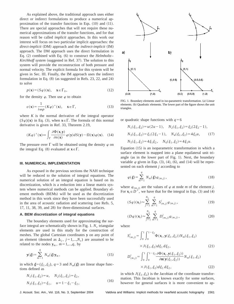
FIG. 2. Sphere of radius 1, center athe origin and 1026 points. The surface is decomposed onto~a! 512 qua-dratic elements and~b! 2048 linear el-ements.

wilatEqg

ththfim

inesamat

g

il

ixd

cugu

dmo

p-

ecala-on

anonbuten-ob-

n-

. 2,

he

ne

ar

n--

eodtionlu-

organized in such a way that the first modes are relatedthe nonevanescent waves and the last modes will be rewith the evanescent waves. The numerical solution of~34! by conventional methodszLS can be represented usinthe SVD as

zLS5@V#diagS 1

s1,...,

1

sN*D @U#Hb̃. ~36!

Notice that this solution will include modes related to bononevanescent and evanescent waves. It is well knownthe modes related to evanescent waves will produce thedetails on the reconstruction, but at the same time will aplify the noise. Special methods for the solution to thisverse acoustic problem will need to include enough of thmodes in order to obtain a certain resolution, and at the stime exclude some of these modes that are contaminwith noise.

The special methods for the solution to Eq.~34! arecalledregularization methodsand can be implemented usinthe SVD as

z̃a5@V#@Fa#diagS 1

s1,...,

1

sN*D @U#Hb̃, ~37!

wherea is known as the regularization parameter and@Fa#is a matrix with diagonal entries called thefilter factor ~seeRefs. 9 and 10!. The parametera will control this inclusionof modes related to evanescent waves into the solutionz̃a .The best known regularization method is Tikhonov and wbe implemented using the filter factor

@Fa#5diagS s12

s121a

,...,sN*

2

sN*2

1aD . ~38!

The topic of regularization methods for linear matrsystems has been extensively studied in the last few decaThere are many other approaches depending on the partiproblem, where we can mention the use of Tikhonov relarization with a high-pass filter~see Ref. 15! which uses thephysical behavior of the evanescent waves to produceoptimal filter. It is not the goal of this work to give a detailestudy of regularization methods for this acoustical problebut instead to provide a fair comparison between the recstruction of the acoustic field given by the implicit a


thed.

atne-

-ee

ed

l

es.lar-

an

,n-

proaches~DM and IM! and the reconstruction given by thtraditional DE approach. For that reason, all of our numeriexperiments in Secs. IV and V will use Tikhonov regulariztion ~which is the oldest and best known regularizatimethod! with the Morozov discrepancy principle~as used inRef. 15! to obtain the optimal parametera.

IV. PROBLEMS WITH THE NUMERICAL SOLUTION

As mentioned previously, the numerical solution toill-posed matrix system will require the use of regularizatimethods, which is itself a subject of current research,there are other problems that will need our particular atttion: the effect of the higher order shape functions and prlematic frequencies.

For the numerical examples in this section, we will cosider the exterior problem of reconstructingvs on the surfaceG, a sphere of radius 1 with 1026 points as shown in Figusing pressure measurementsp over G0 , a sphere of radius1.01 with 1026 points distributed as inG. The vectorp̃ iscreated by adding top the vectore with normal randomdistributed entries and 35 dB SNR.

The figures that will be shown in this section over tsphereG depend on the spherical coordinates (r ,f,u), andhence will be transformed using interpolation into the pla~f,u! for better visualization purposes.

A. Effect of shape functions

The surfaceG can be decomposed using 2048 linetriangular elements as shown in Fig. 2~a! and 512 quadratictriangular elements as shown in Fig. 2~b!. It is a commonpractice for the forward problem to use the quadratic triagular decomposition overG @and so quadratic shape functions on Eq.~18!# in order to improve the accuracy of thsolution to the acoustical problem. This will not be a goidea for the inverse problem, where increasing the resoluwill pay the penalty of reducing the smoothness of the sotion, as we will show.

Let the quantitiesWml , m51,...,3, be defined as

Wml 5E

0

1E0

12j2Nm~j1 ,j2!J~j1 ,j2!dj1 dj2 , ~39!


s

se

r

mn-

u

e-,’’

l

aao

le

int

s,

inl

ar,

totrixfe

ereto

alatndhe

vegu-

rot

forno

henl

nsheicaln

erethem-h

nso-inrti-

nd

tw

for the linear shape functionsNm , given in Eq.~16!. Simi-larly define the quantitiesWm

q , m51,...,6, as

Wmq 5E

0

1E0

12j2Nm~j1 ,j2!J~j1 ,j2!dj1 dj2 , ~40!

for the quadratic shape functionsNm , given in Eq. ~17!.Equations~39! and~40! can be thought of as approximationto S(m, j )

i , D (m, j )i , and K (m, j )

i when the field pointxi is farfrom the elementD j . For our further expositionWm

l andWm

q , instead of being used as an approximation, will be uto estimate the Column normalized weights~CNWs! for thematrices@S#, @D#, @Ss#, @D1#, and@K1#.

The following explanation of the CNW will be given fothe matrix @S#, but will also apply to@D#, @Ss#, @D1#, and@K1#. Notice that@S# is obtained by a reduction of the suof S(m, j )

i in Eq. ~19! and this reduction depends on the triagular elements decomposition used for the surfaceG. Figure3 shows the decomposition of a plane using linear and qdratic triangular elements. Observe in Fig. 3~a! that the‘‘square’’ point ~point marked with a square! intersects sixtriangles. This means that when the sums in Eq.~19! arereduced, then the column of the resultant matrix@S# thatcorresponds to the ‘‘square’’ point will be the sum of thquantitiesS(m, j )

i for j’s andm’s corresponding to the six triangles intersecting the ‘‘square’’ point. For that reasoncolumn of the matrix@S# that corresponds to the ‘‘squarepoint will be associated with the CNW 6Wm

q . Using thesame argument for the ‘‘diamond’’ point in Fig. 3~a!, thecolumn of @S# that corresponds to the ‘‘diamond’’ point wilbe associated with the CNW 2Wm

q . The ‘‘square’’ and ‘‘dia-mond’’ points in the quadratic triangle decomposition ofplane @see Fig. 3~a!# represent, respectively, a vertex andmidpoint of a triangle that belong to the triangular decompsition of G. For that reason, when quadratic triangular e

FIG. 3. Decomposition of a plane using triangular~a! quadratic elementsand ~b! linear elements. The ‘‘square’’ point is the vertex of a triangle aintersects six contiguous triangles for both~a! and~b!. The ‘‘diamond’’ pointin ~a! is the midpoint of a triangle for quadratic elements and intersectscontiguous triangles.


d

a-

a

--

ments are used, the columns of matrices@S# that correspondto a vertex point (m51,2,3) will be associated with theCNW 6Wm

q , and the columns corresponding to a midpo(m54,5,6) will be associated with the CNW 2Wm

q . A simi-lar reasoning will imply that, for linear triangular elementall the columns of@S# are associated with the CNW 6Wm

l

@see Fig. 3~b!#.Notice that this unbalance of the CNW will be found

the entries of the matrix@S# that are outside the diagona~since the field pointsxi in this region are relatively far fromthe elementj!. The worst case is when the surface is plansince the Jacobian on Eq.~40! is constant, then form51, 2,3 we have thatWm

q 50. This will imply that S(m, j )i '0 when

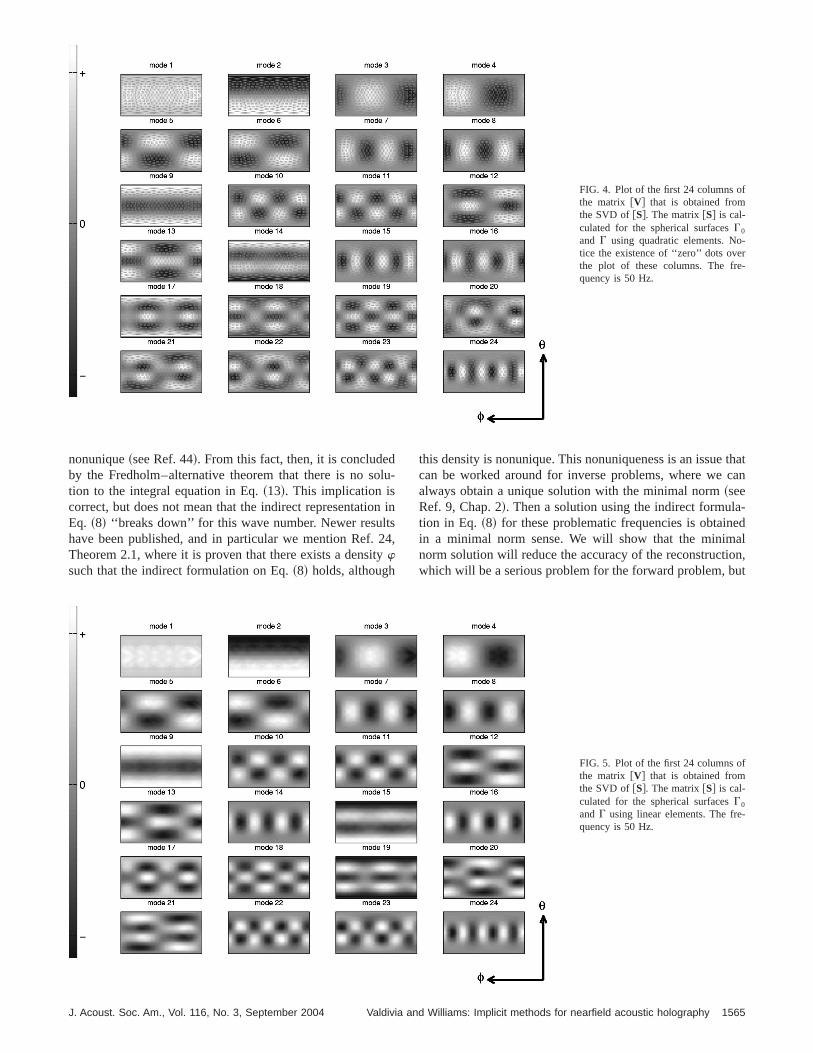
m51, 2, 3, and the matrix@S# will have entries outside thediagonal that are close to 0 for columns that correspondvertex points of quadratic elements. We compute the ma@S# for the spheresG andG0 ~explained in the beginning othis section!, and compute the SVD. As shown in Fig. 4, thunbalance on the columns of@S# will produce ‘‘zero’’ dots onthe plots of the columns of matrix@V#. We can see in Fig. 5that this effect is not encountered for linear elements whthe CNW is balanced. A similar effect will be expectedhappen to the SVD of@Gn#.

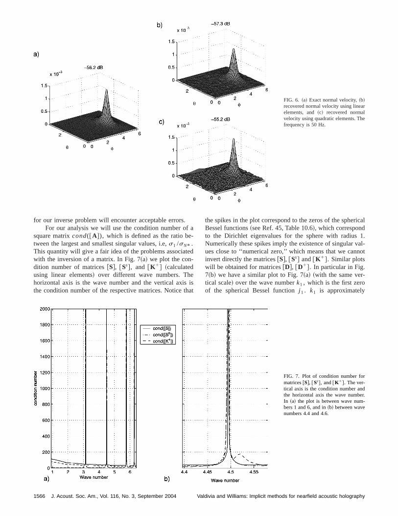
The DE approach will be used to reconstruct the normvelocity vs for 50 Hz given by a point source located~0,20.8,0!. The reconstruction using quadratic elements alinear elements is shown in Fig. 6. The relative error for treconstructed normal velocityvr

s ~given by ivs2vrsi2 /ivsi2

3100%) for the linear elements is 8% while the relatierror for quadratic elements is 28%. In both cases the relarization parameter was chosen to be the optimal~since theexact solution is known!. Notice that the increase in error fothe quadratic elements results from the use of ‘‘zero’’ dmodes for the SVD of@Gn# ~as in the SVD of@S# in Fig. 4!.For the forward problem, where all the modes are usedthe inversion, the use of these quadratic modes will haveeffect in the reconstructed solution~as seen in the literaturefor the forward problem like Ref. 39!. In the inverse prob-lem, where just a partial set of these modes is required, tthe solution will be affected~as shown by our numericaexperiment!.

B. Problematic frequencies

There are certain frequencies where the formulatiodiscussed before will fail to provide a unique solution for tforward problem. This uniqueness is a purely mathematproblem arising from the boundary integral formulatiorather than from the nature of the physical problem. Thare several modified integral formulations to overcomenonuniqueness problem, but in practice the amount of coputational complexity of these formulations will be a higpenalty to pay.

In this section we will clarify a common misconceptiofrom the available acoustical literature in regards to thelution of the exterior problem by the indirect formulationEq. ~8!. For the exterior problem, when the wave numbekcoincides with a Dirichlet eigenvalue, it is known theorecally that the solution to the integral equation in Eq.~13! is

o


-

-

FIG. 4. Plot of the first 24 columns ofthe matrix @V# that is obtained fromthe SVD of@S#. The matrix@S# is cal-culated for the spherical surfacesG0

and G using quadratic elements. Notice the existence of ‘‘zero’’ dots overthe plot of these columns. The frequency is 50 Hz.

dolu

nts2

ty

thatcan

-edalon,ut

nonunique~see Ref. 44!. From this fact, then, it is concludeby the Fredholm–alternative theorem that there is no stion to the integral equation in Eq.~13!. This implication iscorrect, but does not mean that the indirect representatioEq. ~8! ‘‘breaks down’’ for this wave number. Newer resulhave been published, and in particular we mention Ref.Theorem 2.1, where it is proven that there exists a densiwsuch that the indirect formulation on Eq.~8! holds, although


-

in

4,

this density is nonunique. This nonuniqueness is an issuecan be worked around for inverse problems, where wealways obtain a unique solution with the minimal norm~seeRef. 9, Chap. 2!. Then a solution using the indirect formulation in Eq. ~8! for these problematic frequencies is obtainin a minimal norm sense. We will show that the minimnorm solution will reduce the accuracy of the reconstructiwhich will be a serious problem for the forward problem, b

-

FIG. 5. Plot of the first 24 columns ofthe matrix @V# that is obtained fromthe SVD of@S#. The matrix@S# is cal-culated for the spherical surfacesG0

and G using linear elements. The frequency is 50 Hz.


r

e

FIG. 6. ~a! Exact normal velocity,~b!recovered normal velocity using lineaelements, and~c! recovered normalvelocity using quadratic elements. Thfrequency is 50 Hz.

f a-

ed

ei

h

rical

1.al-ot

for our inverse problem will encounter acceptable errors.For our analysis we will use the condition number o

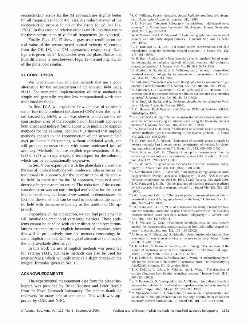
square matrixcond(@A#), which is defined as the ratio between the largest and smallest singular values, i.e,s1 /sN* .This quantity will give a fair idea of the problems associatwith the inversion of a matrix. In Fig. 7~a! we plot the con-dition number of matrices@S#, @Ss#, and @K1# ~calculatedusing linear elements! over different wave numbers. Thhorizontal axis is the wave number and the vertical axisthe condition number of the respective matrices. Notice t


sat

the spikes in the plot correspond to the zeros of the spheBessel functions~see Ref. 45, Table 10.6!, which correspondto the Dirichlet eigenvalues for the sphere with radiusNumerically these spikes imply the existence of singular vues close to ‘‘numerical zero,’’ which means that we canninvert directly the matrices@S#, @Ss# and@K1#. Similar plotswill be obtained for matrices@D#, @D1#. In particular in Fig.7~b! we have a similar plot to Fig. 7~a! ~with the same ver-tical scale! over the wave numberk1 , which is the first zeroof the spherical Bessel functionj 1 . k1 is approximately

r.-

FIG. 7. Plot of condition number formatrices@S#, @Ss#, and@K1#. The ver-tical axis is the condition number andthe horizontal axis the wave numbeIn ~a! the plot is between wave numbers 1 and 6, and in~b! between wavenumbers 4.4 and 4.6.


ro

-

.

FIG. 8. Plot of columns of@V# for thematrix @S# calculated at wave numbek1 which corresponds to the first zerof the spherical Bessel functionj 1 .Notice that the last three columns contain the modes associated withj 1 thatwill not be used for the reconstruction

ig

ann-

pnd

Wechthe

4.492 409 4 and is the second spike from left to right in F7~a!.

The existence of singular values close to ‘‘numericzero’’ will represent a major problem for the explicit creatioof the Green’s matrices for the DE approach, since we caninvert @Ss#, (@D1#2@ I #). It is possible to do a pseudoinversion using the SVD~see Ref. 10!, but this will be costly.The use of implicit methods as the IM approach or DM aproach will not require the explicit inversion of matrices a


.

l

ot

-

for that reason can be applied as explained in Sec. III A.will only compare the reconstructions from the IM approawith the exact solutions, as we expect similar results forDM approach.

Figure 8 shows the plots of some columns of@V# for @S#.Notice that the modes corresponding to the zeros ofj 1

@which are the spherical harmonicsY211 (u,f), Y0

1(u,f),and Y1

1(u,f)] will be at the last columns of@V#. When

FIG. 9. At wave numberk1 , ~a! exact~left! and reconstructed~right! pres-sure and~b! exact ~left! and recon-structed~right! normal velocity.


-

FIG. 10. The parallelepiped surfaceGand arrayG0 used for the physical ex-periment. The surfaceG is decom-posed into 1968 linear triangular elements and 986 points. Themeasurement surfaceG0 have a totalof 805 points~35 in thex direction and23 in they direction!.

luse-a

bu

apere

av

e

eser

rkmryin

-

gha

engo-ec.isill

Tikhonov regularization is applied, this means that our sotion will eliminate the Fourier coefficients pertaining to thomodes. Using the sameG andG0 from the previous subsection, we show in Fig. 9 the reconstruction of the normvelocity at k1 for a point source located at~0,20.8,0!. Thevectorp̃ is created by the addition of a vectore with normalrandom distributed entries and 35 dB SNR. As mentionedthe previous section, we use Tikhonov regularization,since the exact solution is known, we choose the optimregularization parameter. Although the relative error isproximately of 30% for the normal velocity and 20% for thpressure, the principal features of the exact velocity and psure are recovered.

As shown in Fig. 7, there is a spacing between the wnumbersk that coincides with the Dirichlet eigenvalues ofG~or problematic frequencies!. This spacing will becomesmaller as we increase the frequency. In general it is w


-

l

int

al-

s-

e

ll

known33 that there is always a separation between thproblematic frequencies~even if the separation is smaller fohigher frequencies!. For acoustic problems, where we woup to the kHz regime, the probability of choosing a randopositive number that will be a problematic frequency is vesmall. Moreover, we need to construct our linear systemEqs. ~26!, ~27!, ~30!, or ~31! for the exact problematic frequency~at least with several digits of accuracy! to encounter‘‘zero’’ singular values in the SVD of@S#, as was the caseshown in Fig. 8. If that is the case, we have shown throuour numerical example that our reconstruction will suffermoderate loss of accuracy~which is always expected on thinverse problem! due to the loss of the modes correspondito the ‘‘numerical zero’’ singular values. Notice that the prposed implicit methods, applied directly as explained in SIII A for these problematic frequencies, will take care of thcomplication without additional work. The DE approach w

-

0yr

FIG. 11. Gray scale rendition of thereal part of the normal velocity recovered using planar NAH for 24 equallydistributed frequencies between 10Hz and 1.22 kHz. At each frequencwe show the maximum dB level ovethe plate.


re

a

rolieithis

m-

ext,a isan

urcen toghtwasioncm

ionr of

.4ll

th

rd

the

e

z-

x

require special methods for the matrix inversion used to cate the transfer functions@Gd#, @Gn#.

V. PHYSICAL EXPERIMENTS

The experimental configuration for the holographic mesurement is similar to Ref. 46. A steel rectangular plate~of55.9326.7 cm and thickness of 1.6 mm! was driven by aWilcoxon F3/F9 inertial shaker~0 to 3000 Hz! fixed in theunderneath corner of the plate in order to generate a bspectrum of spatial wave numbers. The resulting appforce was used to normalize the pressure measured wACO 7046 1

2-in. microphone above the plate. The scanconducted in an automated point-by-point fashion. Thecrophone is initially positioned by thex-y scanner at a cor

FIG. 12. Plot of % relative error for reconstructions of~a! normal velocityand ~b! pressure. The vertical axis is the % error and the horizontal acorresponds to the frequencies~Hz!.


-

-

adda

i-

ner of the scan area, where the data is then acquired. Nthe microphone is moved to an adjacent point, and datagain acquired. This process is continued until the full scarea is measured. Synchronization between the soshaker, the data acquisition, and the scanner has provehave high stability, yielding coherent data that can be thouof as having been acquired simultaneously. The pressuremeasured on a grid of 69 points along the longer dimensand 46 points along the shorter dimension in a plane 0.4above the plate surface. The step size in both thex and ydirections was 1.25 cm, providing an overall scan dimensof 85357.5 cm. The plate surface is located at the centethis area.

The points on the planar surfaceG0 ~35 points along thex direction and 23 points along they direction! correspond to14 the original pressure measurements~and a spacing in bothx andy directions of 2.5 cm!. G will be a rectangular paral-lelepiped of 70340 cm and thickness of 2.5 cm, located 0cm belowG0 . A uniform spacing of 2.5 cm is used for apoints onG. The spacings over points onG0 andG satisfy theminimal requirements to avoid aliasing when working wifrequencies up to 2 kHz.G0 andG are centered over thex-ycoordinates at~42.5,28.125! cm ~see Fig. 10!. The BEM cal-culation are in MKS units.

In the results which follow, the ‘‘exact’’ normal velocityvs and pressureps on the plate were determined by standaplanar NAH reconstruction using the full 69346 point array.It has been demonstrated that the reconstructions withover-scanned hologram are extremely accurate.1 The use ofthe BEM-NAH approaches discussed in Sec. III A will givthe reconstructed normal velocityvr

s or pressureprs for 24

frequencies distributed equally from 100 Hz to 1.223 kHover the parallelepipedG, but all the comparisons and calculation of errors will be taken over thex-y plane that corre-

is

-

-2

e

FIG. 13. Gray scale rendition of thereal part of the normal velocity recovered using the direct-explicit~DE! ap-proach for 24 equally distributed frequencies between 100 Hz and 1.2kHz. At each frequency we show thmaximum dB level over the plate.


-

2e

FIG. 14. Gray scale rendition of thereal part of the normal velocity recovered using the indirect-implicit~IM !approach for 24 equally distributedfrequencies between 100 Hz and 1.2kHz. At each frequency we show thmaximum dB level over the plate.

o-ar

lu

he

erg.

oth

sponds to the plate@the upperx-y plane onG of dimensions55.9326.7 cm, center on~0.425,0.28125!m#. As mentionedearlier in Sec. III B, Tikhonov regularization using the Morzov discrepancy principle will be used to obtain the regulization parameter for all cases.

Figure 11 shows a gray-scale rendition on the real vaof the ‘‘exact’’ normal velocity vs ~coming from planarNAH! for 24 frequencies that will be used to compute trelative error ivs2vr

si2 /ivsi23100% given in Fig. 12~a!.


-

e

The reconstructed normal velocityvrs will be computed using

the DE, IM, and DM approaches, respectively. Similarly, wuse the ‘‘exact’’ pressureps to compute the relative erroips2pr

si /ipsi3100% on the 24 frequencies given in Fi12~b!. An important property of the error onvr

s reconstruc-tions seen in Fig. 12~a! is that the DE approach and DMapproach give similar errors. This is not surprising since bapproaches use the direct formulation given in Eq.~2!. The

-

2e

FIG. 15. Gray scale rendition of thereal part of the normal velocity recovered using the direct-implicit~DM!approach for 24 equally distributedfrequencies between 100 Hz and 1.2kHz. At each frequency we show thmaximum dB level over the plate.


tte

o

th

chaa

odini

ha

ticatrt

itcieano

En,

haheusalcooth

cop

habuc-

edfo

e

hdithp

s-

iser

of

ld

rily

edst.

e-

e-ting

ldment

bynd

byos-

rust.

g-

rors

1.cted

a inAm.

la-darySoc.

resob-

r-us-

e

-

f

aryral

ndect

reconstruction errors for the IM approach are slightly befor all frequencies~about 4% less!. A similar behavior of thereconstruction error is found on the errors forpr

s @see Fig.12~b!#. In this case the relative error is much less than errfor the reconstruction ofvr

s for all frequencies~as expected!.Finally, Figs. 13–15 show a gray-scale rendition on

real value of the reconstructed normal velocityvrs coming

from the DE, IM, and DM approaches, respectively. Eafigure is given for 24 frequencies over the plate. Notice tlittle difference is seen between Figs. 13–15 and Fig. 11;of the plots look similar.

VI. CONCLUSION

We have shown two implicit methods that are a goalternative for the reconstruction of the acoustic field usNAH. The numerical implementation of these methodssimple and generally requires less computational work ttraditional methods.

In Sec. IV A we explained how the use of quadrashape functions produced unbalanced CNW over the mces created by BEM, which was shown to increase theconstruction error of the acoustic field. This result appliesboth direct and indirect formulations with implicit or explicmethods for the solution. Section IV B showed that implimethods applied to the reconstruction of the acoustic fiover problematic frequencies, without additional work, cstill produce reconstructions with some moderated lossaccuracy. Methods that use explicit representations of~26! or ~27! will require special techniques for the solutiowhich can be computationally expensive.

In Sec. V our experiment with the plate data showed tthe use of implicit methods will produce similar errors as ttraditional DE approach, for the reconstruction of the acotic field. In particular for the IM approach, there is a smdecrease in reconstruction errors. The reduction of the restruction error was not our principal motivation for the useimplicit methods, but instead we wanted to demonstratefact that these methods can be used to reconstruct the atic field with the same efficiency as the traditional DE aproach.

Depending on the application, we can find problems twill involve the creation of very large matrices. These prolems cannot be handled with either direct or indirect formlations that require the explicit inversion of matrices, sinthis will be prohibitively time and memory consuming. Instead implicit methods will be a good alternative~and maybethe only available alternative!.

In this work the use of implicit methods was presentfor exterior NAH, but these methods can also be usedinterior NAH, which will only involve a slight change on thintegral formulas given in Sec. II.

ACKNOWLEDGMENTS

The experimental measurement data from the planarlogram was provided by Brian Houston and Peter Herfrom the Naval Research Laboratory. The authors thankreviewers for many helpful comments. This work was suported by ONR and NRC.


r

rs

e

htll

gsn

ri-e-o

tld

fq.

t

-ln-feus--

t--e

r

o-ce-

1E. G. Williams,Fourier Acoustics: Sound Radiation and Nearfield Acoutical Holography~Academic, London, UK, 1999!.

2J. D. Maynard, ‘‘Acoustic holography for wideband, odd-shaped nosources,’’ in Proceedings Inter-noise ’88, Avignon, France, Septembe1988, Vol. I, pp. 223–231.

3W. A. Veronesi and J. D. Maynard, ‘‘Digital holographic reconstructionsources with arbitrarily shaped surfaces,’’ J. Acoust. Soc. Am.85, 588–598 ~1989!.

4G.-T. Kim and B.-H. Lee, ‘‘3-d sound source reconstruction and fiereprediction using the helmholtz integral equation,’’ J. Sound Vib.136,245–261~1990!.

5M. R. Bai, ‘‘Application of bem~boundary element method!-based acous-tic holography to radiation analysis of sound sources with arbitrashaped geometries,’’ J. Acoust. Soc. Am.92, 533–549~1992!.

6G. Borgiotti, A. Sarkissian, E. G. Williams, and L. Schuetz, ‘‘Generaliznearfield acoustic holography for axisymmetric geometries,’’ J. AcouSoc. Am.88, 199–209~1990!.

7A. Sarkissian, ‘‘Near-field acoustical holography for an axisymmetric gometry: a new formulation,’’ J. Acoust. Soc. Am.88, 961–966~1990!.

8A. Sarkissian, C. F. Gaumond, E. G. Williams, and B. H. Houston, ‘‘Rconstruction of the acoustic field over a limited surface area on a vibracylinder,’’ J. Acoust. Soc. Am.93, 48–54~1993!.

9H. W. Engl, M. Hanke, and A. Neubauer,Regularization of Inverse Prob-lems~Kluwer Academic, Boston, 1996!.

10P. C. Hansen,Rank-Deficient and Discrete Ill-Posed Problems~SIAM,Philadelphia, 1998!.

11B.-K. Kim and J.-G. Ih, ‘‘On the reconstruction of the vibro-acoustic fieover the surface enclosing an interior space using the boundary elemethod,’’ J. Acoust. Soc. Am.100, 3003–3016~1996!.

12P. A. Nelson and S. H. Yoon, ‘‘Estimation of acoustic source strengthinverse methods: Part i, conditioning of the inverse problem,’’ J. SouVib. 233, 643–668~2000!.

13S. H. Yoon and P. A. Nelson, ‘‘Estimation of acoustic source strengthinverse methods: Part ii, experimental investigation of methods for choing regularization parameters,’’ J. Sound Vib.233, 669–705~2000!.

14B.-K. Kim and J.-G. Ih, ‘‘Design of an optimal wave-vector filter foenhancing the resolution of reconstructed source field by nah,’’ J. AcoSoc. Am.107, 3289–3297~2000!.

15E. G. Williams, ‘‘Regularization methods for near-field acoustical holoraphy,’’ J. Acoust. Soc. Am.110, 1976–1988~2001!.

16S. Sureshkumar and S. T. Raveendra, ‘‘An analysis of regularization erin generalized nearfield acoustical holography,’’ in2001 SAE noise andvibration conference, no. 2001-01-1616, Grand Traverse, MI, April 200

17S.-C. Kang and J.-G. Ih, ‘‘On the accuracy of nearfield pressure prediby the acoustic boundary element method,’’ J. Sound Vib.233, 353–358~2000!.

18S.-C. Kang and J.-G. Ih, ‘‘The use of partially measured source datnear-field acoustical holography based on the bem,’’ J. Acoust. Soc.107, 2472–2479~2000!.

19S.-C. Kang and J.-G. Ih, ‘‘Use of nonsingular boundary integral formution for reducing errors due to near-field measurements in the bounelement method based near-field acoustic holography,’’ J. Acoust.Am. 109, 1320–1328~2001!.

20S. F. Wu and X. Zhao, ‘‘Combined helmholtz equation-least squamethod for reconstructing acoustic radiation from arbitrarilty shapedjects,’’ J. Acoust. Soc. Am.112, 179–188~2002!.

21A. Tekatlian, P. Filippi, and D. Habault, ‘‘Determination of vibration chaacteristics of noise sources solving an inverse radiation problem,’’ Actica 82, 91–101~1996!.

22T. K. DeLillo, V. Isakov, N. Valdivia, and L. Wang, ‘‘The detection of thsource of acoustical noise in two dimensions,’’ SIAM~Soc. Ind. Appl.Math.! J. Appl. Math.61~6!, 2104–2121~2001!.

23T. K. Delillo, V. Isakov, N. Valdivia, and L. Wang, ‘‘Computational methods for the detection of the source of acoustical noise,’’ inProceedings ofASME2000, Orlando, FL, November 2000.

24T. K. DeLillo, V. Isakov, N. Valdivia, and L. Wang, ‘‘The detection osurface vibrations from interior acoustical pressure,’’ Inverse Probl.19~3!,507–524~2003!.

25S. T. Raveendra, N. Vlahopoulos, and A. Glaves, ‘‘An indirect boundelement formulation for multi-valued impedance simulation in structuacoustics,’’ Appl. Math. Model.22, 379–393~1998!.

26N. Vlahopoulos and S. T. Raveerdra, ‘‘Formulation, implementation avalidation of multiple connection and free edge constraints in an indirboundary element formulation,’’ J. Sound Vib.201, 137–152~1998!.


hy

B

‘‘Aire

n-fo

ou,’’

ng

ry

nd

latio

t.

-

tic

ceds in

n-

c-

lar

n

larust.

27F. Augusztinovicz, ‘‘Application and extension of acoustic holograptechniques for tire noise investigations,’’ J. Acoust. Soc. Am.105, 1373~1999!.

28E. G. Williams, B. H. Houston, P. C. Herdic, S. T. Raveendra, andGardner, ‘‘Interior nah in flight,’’ J. Acoust. Soc. Am.108, 1451–1463~2000!.

29Z. Zhang, N. Vlahopoulos, S. T. Raveendra, T. Allen, and K. Y. Zhang,computational acoustic field reconstruction process based on an indboundary element formulation,’’ J. Acoust. Soc. Am.108, 2167–2178~2000!.

30Z. Zhang, N. Vlahopoulos, T. Allen, and K. Y. Zhang, ‘‘A source recostruction process based on an indirect variational boundary elementmulation,’’ Eng. Anal. Boundary Elem.25, 93–114~2001!.

31A. Schuhmacher, J. Hald, K. B. Rasmussen, and P. C. Hansen, ‘‘Ssource reconstruction using inverse boundary element calculationsAcoust. Soc. Am.113, 114–126~2003!.

32D. Colton and R. Kress,Inverse Acoustics and Electromagnetic ScatteriTheory~Springer-Verlag, New York, 1992!.

33D. Colton and R. Kress,Integral Equation Methods in Scattering Theo~Wiley-Interscience Publication, New York, 1983!.

34J. Pan and D. A. Bies, ‘‘The effect of fluid-structural coupling on souwaves in an enclosure—theoretical part,’’ J. Acoust. Soc. Am.87, 691–707 ~1990!.

35D. Ouellet, J. L. Guyader, and J. Nicolas, ‘‘Sound field in a rectangucavity in the presence of a thin, flexible obstacle by integral equamethod,’’ J. Acoust. Soc. Am.89, 2131–2139~1991!.


.

ct

r-

ndJ.

rn

36E. G. Williams, ‘‘On Green functions for a cylindrical cavity,’’ J. AcousSoc. Am.102, 3300–3307~1997!.

37T. K. DeLillo, T. Hrycak, and N. Valdivia, ‘‘Iterative regularization methods for inverse problems in acoustics,’’ inProceedings of ASME2002,New Orleans, LA, November 2002.

38C. Langrenne and A. Garcia, ‘‘Integral formulations for the vibroacouscharacterization of a cello,’’ J. Acoust. Soc. Am.105, 1088~1999!.

39A. F. Seybert, B. Soenarko, F. J. Rizzo, and D. J. Shippy, ‘‘An advancomputational method for radiation and scattering of acoustic wavethree dimensions,’’ J. Acoust. Soc. Am.77, 362–368~1985!.

40D. Chien, ‘‘Numerical evaluation of surface integrals in three dimesions,’’ Math. Comput.64~210!, 727–743~1995!.

41K. E. Atkinson,The Numerical Solution of Integral Equations of the Seond Kind ~Cambridge U.P., New York, 1997!.

42A. H. Strout, Approximate Calculation of Multiple Integrals~Prentice–Hall, Englewood Cliffs, NJ, 1971!.

43C. Schwab and W. L. Wendland, ‘‘On numerical cubatures of singusurface integrals in boundary element methods,’’ Numer. Math.62~3!,343–369~1992!.

44H. A. Schenck, ‘‘Improved integral formulation for acoustic radiatioproblems,’’ J. Acoust. Soc. Am.44, 41–58~1968!.

45M. Abramowitz and I. A. Stegun,Handbook of Mathematical Functions,9th ed.~Dover, New York, 1972!.

46E. G. Williams and B. Houston, ‘‘Fast Fourier transform and singuvalue decomposition for patch nearfield acoustical holography,’’ J. AcoSoc. Am.114~3!, 1322–1333~2003!.


Implicit methods of solution to integral formulations in boundary element method based nearfield...

Documents

Transcript of Implicit methods of solution to integral formulations in boundary element method based nearfield...