arX

iv:1

206.

1475

v1 [

phys

ics.

optic

s] 7

Jun

201

2

Shot Noise in Digital Holography

Fadwa Joud, Frederic Verpillat, Michael Atlan, Pierre-Andre Taillard, andMichel Gross

Abstract We discuss on noise in heterodyne holography in an off-axis configuration.We show that, for a weak signal, the noise is dominated by the shot noise on thereference beam. This noise corresponds to an equivalent noise on the signal beamof 1 photo electron per pixel, for the whole sequence of images used to build thedigital hologram.

1 Introduction

Demonstrated by Gabor [1] in the early 50’s, the purpose of holography is to record,on a 2D detector, the phase and the amplitude of the radiationfield scattered byan object under coherent illumination. The photographic film used in conventionalholography is replaced by a 2D electronic detection in digital holography [2] en-

Fadwa JoudLaboratoire Kastler BrosselEcole Normale Superieure , UMR 8552 , UPMC, CNRS 24 rueLhomond , 75231 Paris Cedex 05. e-mail: joud@lkb.ens.fr

Frederic VerpillatLaboratoire Kastler BrosselEcole Normale Superieure , UMR 8552 , UPMC, CNRS 24 rueLhomond , 75231 Paris Cedex 05, e-mail: verpillat@lkb.ens.fr

Michael AtlanFondation Pierre-Gilles de Gennes, Institut Langevin: UMR7587 CNRS, U 979 INSERM, ES-PCI ParisTech, Universite Paris 6, Universite Paris 7, 10rue Vauquelin, 75 231 Paris Cedex 05,France.e-mail: atlan@optique.espci.fr

Pierre-Andre TaillardConservatoire de musique neuchatelois; Avenue Leopold-Robert 34 ; 2300 La Chaux-de-Fonds ;Suisse.e-mail: taillard@hispeed.ch

Michel GrossLaboratoire Kastler BrosselEcole Normale Superieure , UMR 8552 , UPMC, CNRS 24 rueLhomond , 75231 Paris Cedex 05. e-mail: gross@lkb.ens.fr

1

2 Fadwa Joud, Frederic Verpillat, Michael Atlan, Pierre-Andre Taillard, and Michel Gross

abling quantitative numerical analysis. Digital holography has been waiting for therecent development of computer and video technology to be experimentally demon-strated [3]. The main advantage of digital holography is that, contrary to holographywith photographic plates [1], the holograms are recorded bya CCD, and the imageis digitally reconstructed by a computer, avoiding photographic processing [4].

Off-axis holography [5] is the oldest configuration adaptedto digital holography[6, 3, 7]. In off-axis digital holography, as well as in photographic plate holography,the reference or local oscillator (LO) beam is angularly tilted with respect to theobject observation axis. It is then possible to record, witha single hologram, thetwo quadratures of the object’s complex field. However, the object field of viewis reduced, since one must avoid the overlapping of the imagewith the conjugateimage alias [8]. In Phase-shifting digital holography, which has been introducedlater [9], several images are recorded with different LO beam phases. It is thenpossible to obtain the two quadratures of the object field in an in-line configurationeven though the conjugate image alias and the true image overlap, because aliasescan be removed by taking image differences.

We have developed an alternative phase-shifting digital holography technique,called heterodyne holography, that uses a frequency shift of the reference beam tocontinuously shift the phase of the recorded interference pattern [10]. One of theadvantages of this technique is its ability to provide accurate phase shifts that al-low to suppress twin images aliases [11]. This greatly simplifies holographic datahandling, and improves sensitivity. Moreover, it is possible to perform holographicdetection at a frequency different from illumination. One can for example detect”tagged photons” [12, 13] in ultrasound-modulated opticalimaging [14]. One canalso also image vibrating objects at the frequencies corresponding to vibration side-bands [15, 16]. To the end, it is possible to perform Laser Doppler imaging [17]within microvessels [18, 19, 20].

More generally, our setup can be viewed as a multipixel heterodyne detector thatis able of recording the complex amplitude of the signal electromagnetic fieldEonto all pixels of the CCD camera in parallel. We get the map ofthe field over thearray detector (i.e.E (x,y) wherex andy are the pixels coordinates). Since the fieldis measured on all pixels at the same time, the relative phasethat is measured fordifferent locations(x,y) is meaningful. This means that the field mapE (x,y) is ahologram that can be used to reconstruct the fieldE in any location, in particular inthe object plane.

In the present paper we will discuss on noise in digital holography, and we willtry to determine what is the ultimate noise limit both theoretically, and in real timeholographic experiments. We will see that, in the theoretical ideal case, the lim-iting noise is the Shot Noise on the holographic reference beam. In reference toheterodyne detection, the reference beam is also called Local Oscillator. We willsee that the ultimate theoretical limiting noise can be reached in real time holo-graphic experiment, by using heterodyne holography [10] inoff-axis configuration.This combination makes possible to fully filter off the technical noise, whose mainorigin is the LO beam technical noise, opening the way to holography with ultimatesensitivity [21, 22].

Shot Noise in Digital Holography 3

2 Theoretical noise

To discuss on noise in digital digital holography, we will consider both the case ofoff-axis holography, where the hologram is obtained from one frame of the CCDcamera, and the case of phase shifting holography, where theholographic informa-tion is extracted from a sequence ofM frames.

We will thus consider a sequence ofM frames:I0 to IM−1 (whereM = 1 inthe one shot, off axis case). For each frameIk, let us noteIk,p,q the CCD camerasignal on each pixel, wherek is the frame index, andp,q the pixel indexes alongthe x andy directions. The CCD signalIk,p,q is measured in Digital Counts (DC)units. In the typical case of the 12 bit digital camera used inexperiments below, wehave 0≤ Ik,p,q < 4096. For each framek, the optical signal is integrated by overthe acquisition timeT = 1/ fccd of the CCD camera. The pixel signalIk,p,q is thusdefined by :

Ik,p,q =

∫ tk+T/2

tk−T/2dt

∫ ∫

(p,q)dxdy |E(x,y, t)+ELO(x,y, t)|

2 (1)

where∫ ∫

(p,q)dxdy represents the integral over the pixel(p,q) area, and wheretk isthe recording moment of framek. Introducing the complex representationsE andELO of the fieldsE andELO, we get :

E(x,y, t) = E (x,y)e jωIt + c.c. (2)

ELO(x,y, t) = ELO(x,y)ejωLOt + c.c (3)

Ik,p,q = a2T(

|Ep,q|2+ |ELO|

2+Ep,qE∗LO · e( j(ωI−ωLO)tk)+ c.c.

)

(4)

wherea is the pixel size. To simplify the notations in Eq.4, we have considered thatthe LO fieldELO is the same in all locations(x,y), and that signal fieldEp,q does notvary within the pixel(p,q). If ELO varies with location, one has to replaceELO byELO,p,q in Eq.4.

In the single-shot, off-axis holography case, the hologramH is simplyH ≡ Ik. Inorder to simplify the discussion in the phase shifting digital holography case [9], wewill consider 4 phases holographic detection (M = 4n). In that case, the phase shiftof the LO beam equal toπ/2 from one recorded frame to the next. Because of thisshift, the complex hologramH is obtained by summing the sequence ofM framesI1 to IM with the appropriate phase coefficient :

H ≡M

∑k=1

( j)k−1Ik (5)

whereH is a matrix of pixelHp,q, and whereM = 4n in the 4-phases phase-shiftingcase, andM = 1 in the single-shot, off-axis case. We get from Eq.4 :

4 Fadwa Joud, Frederic Verpillat, Michael Atlan, Pierre-Andre Taillard, and Michel Gross

Hp,q =M

∑k=1

( j)kIk,p,q = 4na2TEp,qE∗LO (6)

The complex hologramHp,q is thus proportional to the object fieldEp,q with a pro-portionality factor that involvesE ∗

LO.

2.1 The Shot Noise on the CCD pixel signal

Because of spontaneous emission, laser emission and photodetection are randomprocesses, the signal that is obtained on a CCD pixel exhibits a Poisson noise called”shot noise”. The effect of this Poisson noise on the signal,and on the holographicimages, is the Ultimate Theoretical Limiting noise, which we will study here.

We can split the signalIk,p,q: we get for framek and pixel(p,q), in a noiselessaverage component〈Ik,p,q〉 (here〈 〉 is the statistical average operator) and a noisecomponentik,p,q:

Ik,p,q ≡ 〈Ik,p,q〉+ ik,p,q (7)

To go further in the discussion, we will use photo electrons Units to measure thesignalIk,p,q.

We must notice that the local oscillator signalELO is large, and corresponds to alarge number of photo electrons (e). In real life, this assumption is true. For example,if we adjust the power of the LO beam to be at the half maximum for the camerasignal in DC unit (2048 DC for a 12 bits camera), the pixel signal will be about104 e for the camera used below in experiments, since the ”CameraGain” is 4.8 eper DC. This yields two consequences, which simplify the analysis. First, the signalIk,p,q exhibits a gaussian distribution around its statistical average. Second, both thequantization noise of the photo electron signal (Ik,p,q is an integer in photo electronUnits), and the quantization noise of the Digital Count signal (Ik,p,q is an integer inDC Units) can be neglected. These approximations are valid,since the width of theIk,p,q gaussian distribution is much larger than one in both photo electron and DCUnits. In the example given above,〈Ik,p,q〉 ≃ 104, and this width is≃ 102 in photoelectron Units, and≃ 20 in DC Units. One can thus consider thatIk,p,q, 〈Ik,p,q〉 andik,p,q are floating numbers (and not integer). Moreover,ik,p,q is a random Gaussiandistribution, with :

〈ik,p,q〉= 0 (8)

〈i2k,p,q〉= 〈Ik,p,q〉 (9)

To analyse the shot noise’s contribution to the holographicsignalHp,q, one ofthe most simple method is to perform Monte Carlo simulation from Eq.7, Eq.8 andEq.9. SinceIk,p,q is ever large in real life (about 104 in our experiment),〈Ik,p,q〉 canbe replaced byIk,p,q (which is measured in experiment) in the right member of Eq.9.One has thus:

〈i2k,p,q〉= 〈Ik,p,q〉 ≃ Ik,p,q (10)

Shot Noise in Digital Holography 5

Monte Carlo simulation of the noise can be done from Eq.7, Eq.8 and Eq.10

2.2 The Object field Equivalent Noise for 1 frame

Fig. 1 1 photon equivalentsignal (accounting Hetero-dyne gain), and shot noiseon the holographic LocalOscillator beam.

In order to discuss the effect of the shot noise on the heterodyne signalEp,qE∗LO

of Eq.4, let us consider the simple situation sketched on Fig.1. A weak object fieldE, with 1 photon or 1 photo electron per pixel and per frame, interferes with a LOfield ELO with N photons, whereN is large (N = 104, in the case of our experiment).Since the LO beam signala2T |ELO|

2 is equal toN photons, and the object fieldsignala2T |Ep,q|

2 is one photon, we have:

Ik,p,q = N +1+ ik,p,q+ a2TEp,qE∗LOe...+ c.c. (11)

The heterodyne signalEp,qE∗LO is much larger than|Ep,q|

2. This is the gain effect,associated to the coherent detection of the fieldEp,q. This gain is commonly called”heterodyne gain”, and is proportional to the amplitude of the LO fieldE

∗LO.

The purpose of the present discussion is to determine the effect of the noiseterm ik,p,q in Eq.11 on the holographic signalHp,q. SinceHp,q involves only theheterodyne termEp,qE

∗LO (see Eq.6), we have to compare, in Eq.11, the shot noise

termik,p,q, and the heterodyne termEp,qE∗LO.

Consider first the shot noise term. We have

〈i2k,p,q〉= 〈Ik,p,q〉= N +1≃ N (12)

The variance of the shot noise term is thusN1/2. Since this noise is mainly relatedto the shot noise on the local oscillator (sinceN ≫ 1), one can group together, inEq.11, the LO beam term (i.e.N) with the noise termik,p,q, and consider that the LObeam signal fluctuates, the number of LO beam photons being thus ”N ±N1/2”, asmentioned on Fig.1.

Consider now the the heterodyne beat signal. Since we haveN photons on theLO beam, and 1 photon on the object beam, we get:

a2T |Ep,qE∗LO| ≡

((

a2T |E p,q|2)

(

a2T |E LO|2))1/2

= N1/2 (13)

The heterodyne beat signalEp,qE∗LO is thusN1/2 = 100.

6 Fadwa Joud, Frederic Verpillat, Michael Atlan, Pierre-Andre Taillard, and Michel Gross

The shot noise termik,p,q is thus equal to the heterodyne signalEp,qE∗LO corre-

sponding to 1 photon on the object field. This means that shot noiseik,p,q yields anequivalent noise of 1 photon per pixel, on the object beam. This result is obtainedhere for 1 frame. We will show that it remains true for a sequence of M frames,whateverM = 4n is.

2.3 The Object field Equivalent Noise forM = 4n frames

Let us introduce the DC component signalD, which is similar to the heterodynesignalH given by Eq.5, but without phase factors:

D ≡M

∑k=1

Ik (14)

The componentD can be defined for each pixel(p,q) by :

Dp,q ≡M

∑k=1

Ik,p,q (15)

SinceIk,p,q is always large in real life (about 104 in our experiment), the shot noiseterm can be neglected in the calculation ofDp,q by Eq.15. We have thus:

Dp,q ≡M

∑k=1

Ik,p,q = Ma2T(

|Ep,q|2+ |ELO|

2) (16)

We are implicitly interested by the low signal situation (i.e. Ep,q ≪ ELO ) becausewe focus on noise analysis. In that case, the|Ep,q|

2 term can be neglected in Eq.16.This means thatDp,q gives a good approximation for the LO signal.

Dp,q ≡M

∑k=1

Ik,p,q ≃ Ma2T |ELO|2 (17)

We can get then the signal field|Ep,q|2 from Eq.6 and Eq.17:

|Hp,q|2

Dp,q≃ Ma2T |Ep,q|

2 (18)

In this equation, the ratio|Hp,q|2/Dp,q is proportional to the number of frames of the

sequence (M = 4n), This means that|Hp,q|2/Dp,q represents the signal field|Ep,q|

2

summed over the all frames.Let us calculate the effect of the shot noise on|Hp,q|

2/Dp,q. To calculate thiseffect, one can make a Monte Carlo simulation as mentioned above, but a simplercalculation can be done here. Let us develop|Hp,q| in statistical average and noise

Shot Noise in Digital Holography 7

components (as done forIk,p,q in Eq.7):

Hp,q = 〈Hp,q〉+ hp,q (19)

with

hp,q =4n

∑k=1

j kik,p,q (20)

Let us calculate〈|Hp,q|2/Dp,q〉 from Eq.18. SinceDp,q ≃ 〈Dp,q〉, we get :

⟨

|Hp,q|2

Dp,q

⟩

≃|〈Hp,q〉|

2+ 〈|hp,q|2〉+ 〈〈Hp,q〉h∗p,q〉+ 〈〈H∗

p,q〉hp,q〉

〈Dp,q〉(21)

In Eq.21 the〈〈Hp,q〉h∗p,q〉 term is zero sinceh∗p,q is random while〈Hp,q〉 is not. Thetwo terms〈〈Hp,q〉h∗p,q〉 and〈〈H∗

p,q〉hp,q〉 can be thus removed. On the other hand, weget for|hp,q|

2

|hp,q|2 =

4n

∑k=1

|ik,p,q|2+

4n

∑k=1

4n

∑k′=1,k′ 6=k

j k−k′ ik,p,qik′,p,q (22)

Sinceik,p,q andik′,p,q are uncorrelated, theik,p,qik′,p,q terms cancel in the calculationof the statistical average of|hp,q|

2. We get then from Eq.9

〈|hp,q|2〉=

4n

∑k=1

〈|ik,p,q|2〉=

4n

∑k=1

〈Ik,p,q〉= 〈Dp,q〉 (23)

Eq.21 becomes thus :⟨

|Hp,q|2

Dp,q

⟩

=|〈Hp,q〉|

2

〈Dp,q〉+1 (24)

Equation 24 means that the average detected intensity signal 〈|Hp,q|2/Dp,q〉 is the

sum of the square of the average object field〈|Hp,q|〉/(〈Dp,q〉1/2) plus one photo-

electron. Without illumination of the object, the average object field is zero, andthe detected signal is 1 photo-electron. The equation establishes thus that the LOshot noise yields a signal intensity corresponding exactlyto 1 photo-electron (e) perpixel.

The 1 e noise floor, we get here, can be also interpreted as resulting from theheterodyne detection of the vacuum field fluctuations [23].

3 Reaching the Shot Noise in real life holographic experiment.

In section 2, we have shown that the theoretical noise on the holographic recon-structed intensity images is 1 photo electron per pixel whatever the number of

8 Fadwa Joud, Frederic Verpillat, Michael Atlan, Pierre-Andre Taillard, and Michel Gross

recorded frames is. We will now discuss the ability to reach this limit in real timeholographic experiment. Since we consider implicitly a very weak object beam sig-nal (E ≪ ELO ), the noises that must be considered are the readout noise ofthe CCDcamera, the technical noise from laser amplitude fluctuations on the LO beam, andthe LO beam shot noise, which yields the theoretical noise limit.

Consider a typical holographic experiment made with a PCO Pixelfly 12 bit dig-ital camera. The LO beam power is adjusted in order to be at half saturation of thedigital camera output. Since the camera is 12 bits, and sincethe camera ”gain” is4.8e/DC, half saturation corresponds to 2000 DC on the A/D Converter, i.e. about104 e on the each CCD pixel . The LO shot noise, which is about 100 e,is thus muchlarger than the Pixelfly Read Noise (20 e), Dark Noise (3 e/sec) and A/D quantiza-tion noise (4.8 e, since 1 DC corresponds to 4.8 e). The noise of the camera can beneglected, and is not a limiting factor for reaching the noise theoretical limit.

The LO beam that reaches the camera is essentially flat field (i.e. the field in-tensity|ELO|

2 is roughly the same for all the pixels). The LO beam technicalnoiseis thus highly correlated in all pixels. This is in particular the case for the noiseinduced by the fluctuations of the main laser intensity, or bythe vibrations of themirrors within the LO beam arm. To illustrate this point, we have recorded a se-quence ofM = 4n = 4 framesIk (with k = 0...3) with a LO beam, but without signalfrom the object (i.e. without illumination of the object). We have thus recorded thehologram of the ”vacuum field”. We have calculated then the complex hologramH(x,y) by Eq.5, and the reciprocal space hologramH(kx,ky) by Fourier transform:

H(kx,ky) = FFT H(x,y) (25)

Fig. 2 Intensity image ofH(kx,ky,0) for M = 4n = 4frames without illuminationof the object (no signal fieldE ). Three kind of noises canbe identified. Down left (1) :shot noise; center (2): techni-cal noise of the CCD; left (3): FFT aliasing. By truncatingthe image and keeping onlythe left down part, the shotnoise limit is reached. Theimage is displayed in arbitrarylogarithm grey scale.

The reciprocal space holographic intensity|H|2 is displayed on Fig.2 in arbi-trary logarithm grey scale. On most of the reciprocal space (within for example cir-cle 1),|H|2 corresponds to a random speckle whose average intensity is uniformlydistributed alongkx andky. One observes nevertheless bright points within circle2, which corresponds to(kx,ky) ≃ (0,0). These points correspond to the technical

Shot Noise in Digital Holography 9

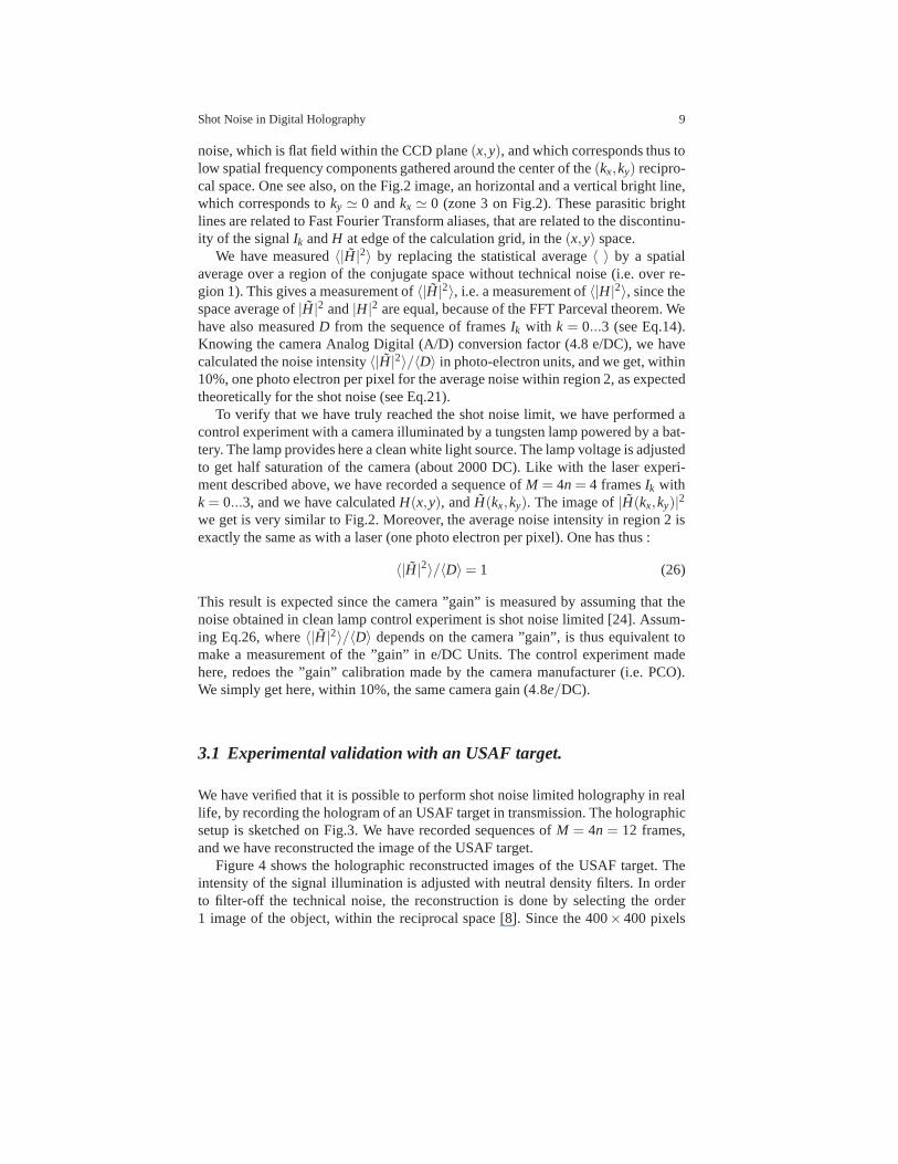
noise, which is flat field within the CCD plane(x,y), and which corresponds thus tolow spatial frequency components gathered around the center of the(kx,ky) recipro-cal space. One see also, on the Fig.2 image, an horizontal anda vertical bright line,which corresponds toky ≃ 0 andkx ≃ 0 (zone 3 on Fig.2). These parasitic brightlines are related to Fast Fourier Transform aliases, that are related to the discontinu-ity of the signalIk andH at edge of the calculation grid, in the(x,y) space.

We have measured〈|H|2〉 by replacing the statistical average〈 〉 by a spatialaverage over a region of the conjugate space without technical noise (i.e. over re-gion 1). This gives a measurement of〈|H|2〉, i.e. a measurement of〈|H|2〉, since thespace average of|H|2 and|H|2 are equal, because of the FFT Parceval theorem. Wehave also measuredD from the sequence of framesIk with k = 0...3 (see Eq.14).Knowing the camera Analog Digital (A/D) conversion factor (4.8 e/DC), we havecalculated the noise intensity〈|H|2〉/〈D〉 in photo-electron units, and we get, within10%, one photo electron per pixel for the average noise within region 2, as expectedtheoretically for the shot noise (see Eq.21).

To verify that we have truly reached the shot noise limit, we have performed acontrol experiment with a camera illuminated by a tungsten lamp powered by a bat-tery. The lamp provides here a clean white light source. The lamp voltage is adjustedto get half saturation of the camera (about 2000 DC). Like with the laser experi-ment described above, we have recorded a sequence ofM = 4n = 4 framesIk withk = 0...3, and we have calculatedH(x,y), andH(kx,ky). The image of|H(kx,ky)|

2

we get is very similar to Fig.2. Moreover, the average noise intensity in region 2 isexactly the same as with a laser (one photo electron per pixel). One has thus :

〈|H|2〉/〈D〉= 1 (26)

This result is expected since the camera ”gain” is measured by assuming that thenoise obtained in clean lamp control experiment is shot noise limited [24]. Assum-ing Eq.26, where〈|H|2〉/〈D〉 depends on the camera ”gain”, is thus equivalent tomake a measurement of the ”gain” in e/DC Units. The control experiment madehere, redoes the ”gain” calibration made by the camera manufacturer (i.e. PCO).We simply get here, within 10%, the same camera gain (4.8e/DC).

3.1 Experimental validation with an USAF target.

We have verified that it is possible to perform shot noise limited holography in reallife, by recording the hologram of an USAF target in transmission. The holographicsetup is sketched on Fig.3. We have recorded sequences ofM = 4n = 12 frames,and we have reconstructed the image of the USAF target.

Figure 4 shows the holographic reconstructed images of the USAF target. Theintensity of the signal illumination is adjusted with neutral density filters. In orderto filter-off the technical noise, the reconstruction is done by selecting the order1 image of the object, within the reciprocal space [8]. Sincethe 400×400 pixels

10 Fadwa Joud, Frederic Verpillat, Michael Atlan, Pierre-Andre Taillard, and Michel Gross

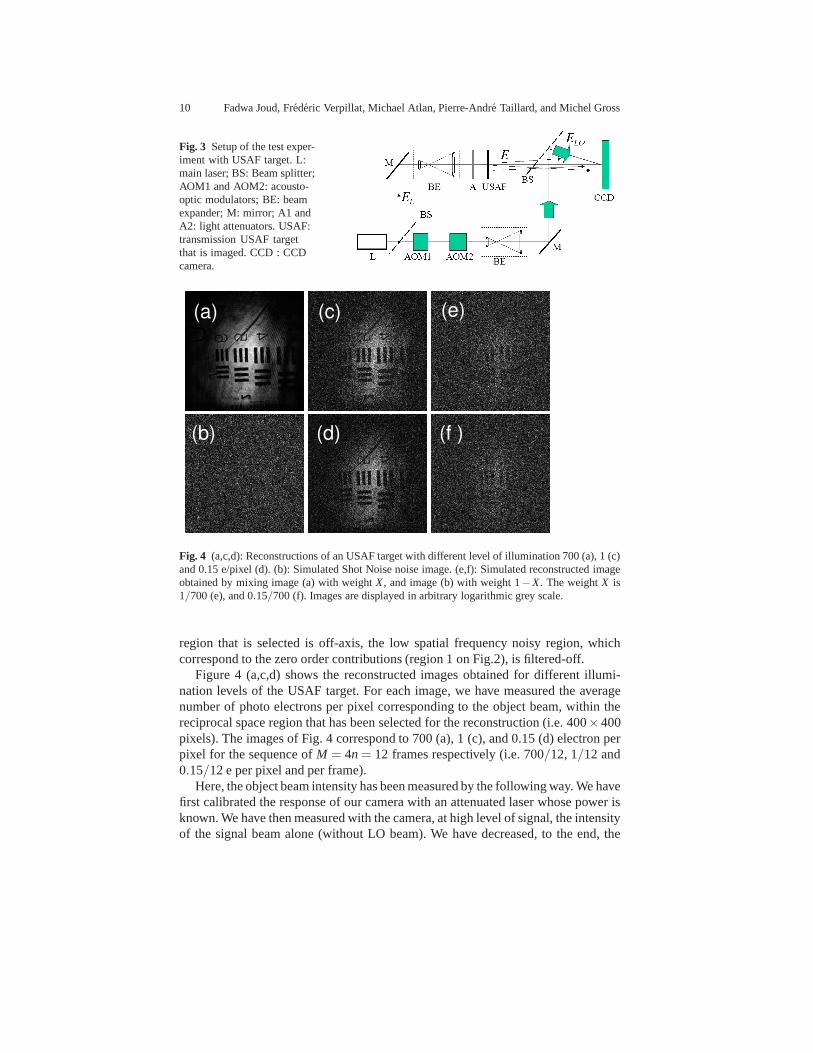
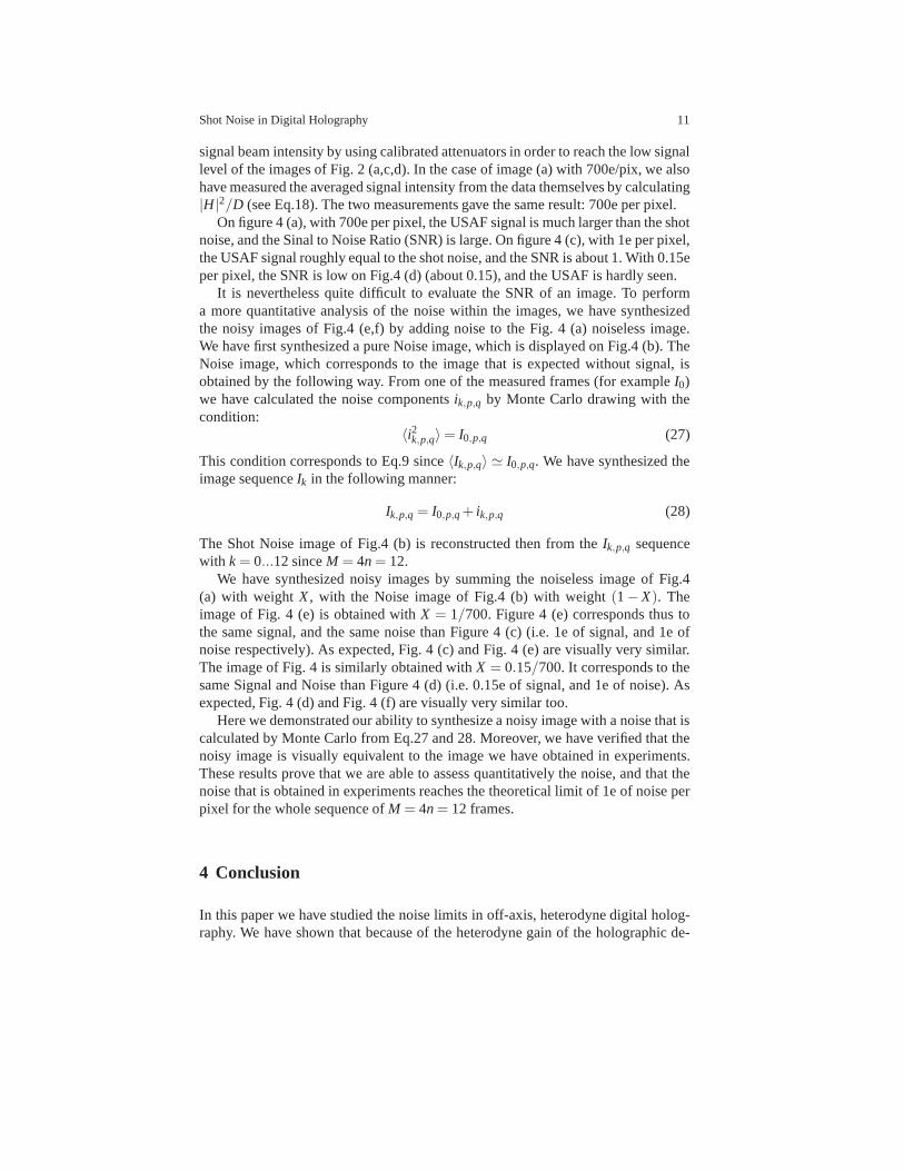
Fig. 3 Setup of the test exper-iment with USAF target. L:main laser; BS: Beam splitter;AOM1 and AOM2: acousto-optic modulators; BE: beamexpander; M: mirror; A1 andA2: light attenuators. USAF:transmission USAF targetthat is imaged. CCD : CCDcamera.

(a) (c) (e)

(b) (d) (f )

Fig. 4 (a,c,d): Reconstructions of an USAF target with different level of illumination 700 (a), 1 (c)and 0.15 e/pixel (d). (b): Simulated Shot Noise noise image.(e,f): Simulated reconstructed imageobtained by mixing image (a) with weightX , and image (b) with weight 1−X . The weightX is1/700 (e), and 0.15/700 (f). Images are displayed in arbitrary logarithmic greyscale.

region that is selected is off-axis, the low spatial frequency noisy region, whichcorrespond to the zero order contributions (region 1 on Fig.2), is filtered-off.

Figure 4 (a,c,d) shows the reconstructed images obtained for different illumi-nation levels of the USAF target. For each image, we have measured the averagenumber of photo electrons per pixel corresponding to the object beam, within thereciprocal space region that has been selected for the reconstruction (i.e. 400×400pixels). The images of Fig. 4 correspond to 700 (a), 1 (c), and0.15 (d) electron perpixel for the sequence ofM = 4n = 12 frames respectively (i.e. 700/12, 1/12 and0.15/12 e per pixel and per frame).

Here, the object beam intensity has been measured by the following way. We havefirst calibrated the response of our camera with an attenuated laser whose power isknown. We have then measured with the camera, at high level ofsignal, the intensityof the signal beam alone (without LO beam). We have decreased, to the end, the

Shot Noise in Digital Holography 11

signal beam intensity by using calibrated attenuators in order to reach the low signallevel of the images of Fig. 2 (a,c,d). In the case of image (a) with 700e/pix, we alsohave measured the averaged signal intensity from the data themselves by calculating|H|2/D (see Eq.18). The two measurements gave the same result: 700eper pixel.

On figure 4 (a), with 700e per pixel, the USAF signal is much larger than the shotnoise, and the Sinal to Noise Ratio (SNR) is large. On figure 4 (c), with 1e per pixel,the USAF signal roughly equal to the shot noise, and the SNR isabout 1. With 0.15eper pixel, the SNR is low on Fig.4 (d) (about 0.15), and the USAF is hardly seen.

It is nevertheless quite difficult to evaluate the SNR of an image. To performa more quantitative analysis of the noise within the images,we have synthesizedthe noisy images of Fig.4 (e,f) by adding noise to the Fig. 4 (a) noiseless image.We have first synthesized a pure Noise image, which is displayed on Fig.4 (b). TheNoise image, which corresponds to the image that is expectedwithout signal, isobtained by the following way. From one of the measured frames (for exampleI0)we have calculated the noise componentsik,p,q by Monte Carlo drawing with thecondition:

〈i2k,p,q〉= I0,p,q (27)

This condition corresponds to Eq.9 since〈Ik,p,q〉 ≃ I0,p,q. We have synthesized theimage sequenceIk in the following manner:

Ik,p,q = I0,p,q + ik,p,q (28)

The Shot Noise image of Fig.4 (b) is reconstructed then from the Ik,p,q sequencewith k = 0...12 sinceM = 4n = 12.

We have synthesized noisy images by summing the noiseless image of Fig.4(a) with weightX , with the Noise image of Fig.4 (b) with weight(1− X). Theimage of Fig. 4 (e) is obtained withX = 1/700. Figure 4 (e) corresponds thus tothe same signal, and the same noise than Figure 4 (c) (i.e. 1e of signal, and 1e ofnoise respectively). As expected, Fig. 4 (c) and Fig. 4 (e) are visually very similar.The image of Fig. 4 is similarly obtained withX = 0.15/700. It corresponds to thesame Signal and Noise than Figure 4 (d) (i.e. 0.15e of signal,and 1e of noise). Asexpected, Fig. 4 (d) and Fig. 4 (f) are visually very similar too.

Here we demonstrated our ability to synthesize a noisy imagewith a noise that iscalculated by Monte Carlo from Eq.27 and 28. Moreover, we have verified that thenoisy image is visually equivalent to the image we have obtained in experiments.These results prove that we are able to assess quantitatively the noise, and that thenoise that is obtained in experiments reaches the theoretical limit of 1e of noise perpixel for the whole sequence ofM = 4n = 12 frames.

4 Conclusion

In this paper we have studied the noise limits in off-axis, heterodyne digital holog-raphy. We have shown that because of the heterodyne gain of the holographic de-

12 Fadwa Joud, Frederic Verpillat, Michael Atlan, Pierre-Andre Taillard, and Michel Gross

tection, the noise of the CCD camera can be neglected. Moreover by a proper ar-rangement of the holographic setup, that combines off-axisgeometry with phaseshifting acquisition of holograms by heterodyne holography, it is possible to reachthe theoretical shot noise limit. We have studied theoretically this limit, and we haveshown that it corresponds to 1 photo electron per pixel for the whole sequence offrame that is used to reconstruct the holographic image. This paradoxical result isrelated to the heterodyne detection, where the detection bandwidth is inversely pro-portional to the measurement time. We have verified all our results experimentally,and we have shown that is possible to image objects at very lowsignal levels. Wehave also shown that is possible to mimic the very weak illumination levels holo-grams obtained in experiments by Monte Carlo noise modeling.

References

1. D. Gabor. Microscopy by reconstructed wavefronts.Proc. R. Soc. A, 197:454, 1949.2. A. Macovsky. Consideration of television holography.Optica Acta, 22(16):1268, August

1971.3. U. Schnars. Direct phase determination in hologram interferometry with use of digitally

recorded holograms.JOSA A., 11:977, July 1994.4. J. W. Goodmann and R. W. Lawrence. Digital image formationfrom electronically detected

holograms.Appl. Phys. Lett., 11:77, 1967.5. E.N. Leith, J. Upatnieks, and K.A. Haines. Microscopy by wavefront reconstruction.Journal

of the Optical Society of America, 55(8):981–986, 1965.6. U. Schnars and W. Juptner. Direct recording of hologramsby a CCD target and numerical

reconstruction.Appl. Opt., 33(2):179–181, 1994.7. T. M. Kreis, W. P. O. Juptner, and J. Geldmacher. Principles of digital holographic interfer-

ometry.SPIE, 3478:45, July 1988.8. Etienne Cuche, Pierre Marquet, and Christian Depeursinge. spatial filtering for zero-order and

twin-image elimination in digital off-axis holography.Appl. Opt., 39(23):4070–4075, 2000.9. I. Yamaguchi and T. Zhang. Phase-shifting digital holography.Optics Letters, 18(1):31, 1997.

10. F. LeClerc, L. Collot, and M. Gross. Numerical heterodyne holography using 2d photo-detector arrays.Optics Letters, 25:716, Mai 2000.

11. M. Atlan, M. Gross, and E. Absil. Accurate phase-shifting digital interferometry. Opticsletters, 32(11):1456–1458, 2007.

12. M. Gross, P. Goy, and M. Al-Koussa. Shot-noise detectionof ultrasound-tagged photons inultrasound-modulated optical imaging.Optics letters, 28(24):2482–2484, 2003.

13. M. Atlan, BC Forget, F. Ramaz, AC Boccara, and M. Gross. Pulsed acousto-optic imag-ing in dynamic scattering media with heterodyne parallel speckle detection.Optics letters,30(11):1360–1362, 2005.

14. L. Wang and X. Zhao. Ultrasound-modulated optical tomography of absorbing objects buriedin dense tissue-simulating turbid media.Applied optics, 36(28):7277–7282, 1997.

15. F. Joud, F. Laloe, M. Atlan, J. Hare, and M. Gross. Imaginga vibrating object by SidebandDigital Holography.Optics Express, 17:2774, 2009.

16. F. Joud, F. Verpillat, F. Laloe, M. Atlan, J. Hare, and M.Gross. Fringe-free holographicmeasurements of large-amplitude vibrations.Optics Letters, 34(23):3698–3700, 2009.

17. M. Atlan, M. Gross, and J. Leng. Laser Doppler imaging of microflow. J. Eur. Opt. Soc. RapidPublications, 1:06025–1, 2006.

18. M. Atlan, M. Gross, BC Forget, T. Vitalis, A. Rancillac, and AK Dunn. Frequency-domainwide-field laser Doppler in vivo imaging.Optics letters, 31(18):2762–2764, 2006.

Shot Noise in Digital Holography 13

19. M. Atlan, B.C. Forget, A.C. Boccara, T. Vitalis, A. Rancillac, A.K. Dunn, and M. Gross.Cortical blood flow assessment with frequency-domain laserDoppler microscopy.Journal ofBiomedical Optics, 12:024019, 2007.

20. M. Atlan, M. Gross, T. Vitalis, A. Rancillac, J. Rossier,and AC Boccara. High-speed wave-mixing laser Doppler imaging in vivo.Optics Letters, 33(8):842–844, 2008.

21. M. Gross and M. Atlan. Digital holography with ultimate sensitivity. Optics Letters,32(8):909–911, 2007.

22. M. Gross, M. Atlan, and E. Absil. Noise and aliases in off-axis and phase-shifting holography.Applied Optics, 47(11):1757–1766, 2008.

23. H.A. Bachor, T.C. Ralph, S. Lucia, and T.C. Ralph.A guide to experiments in quantum optics.wiley-vch, 1998.

24. M. Newberry. Measuring the Gain of a CCD Camera.Axiom Technical Note: 1, 1:1–9, 1998-2000.