LOVELOCK GRAVITY, BLACK HOLES AND HOLOGRAPHY
284
Departamento de F´ ısica de Part´ ıculas LOVELOCK GRAVITY, BLACK HOLES AND HOLOGRAPHY Xi´ an Otero Cama˜ no TESE DE DOUTORAMENTO arXiv:1509.08129v1 [hep-th] 27 Sep 2015
-
Upload
khangminh22 -
Category
Documents
-
view
3 -
download
0
Transcript of LOVELOCK GRAVITY, BLACK HOLES AND HOLOGRAPHY
Departamento de Fısica de Partıculas
LOVELOCK GRAVITY, BLACK HOLES
AND HOLOGRAPHY
Xian Otero Camano
TESE DE DOUTORAMENTO
arX
iv:1
509.
0812
9v1
[he
p-th
] 2
7 Se
p 20
15

UNIVERSIDADE DE SANTIAGO DE COMPOSTELA
Departamento de Fısica de Partıculas
LOVELOCK GRAVITY, BLACK HOLES& HOLOGRAPHY
Xian Otero CamanoPhD supervisor: Jose D. Edelstein Glaubach
Santiago de Compostela, May 20131.
1[Revised: minor corrections, updated references] Berlin, September 2015.

“Unha serea que canta de noite polos tellados, e un astronauta en bicicletaque no asomar das estrelas ven beijarlle as palmas das mans. Nese intre, noespello frıo da lua acendes a noite, e ardemos. Eu creo que foi ası como naceu oUniverso”
[Patrieira, Big Bang]
A todos os que confiaron en min, mais do que eu mesmo.
v

“We are like dwarfs standing upon the shoulders of giants,and so able to see more and see farther than the ancients.”
Bernard of Chartres
Agradecementos
. . . e ate aquı chegou o camino, un ronsel entre tantos, fin de etapa, porto de abrigo. Tempode ollar atras antes do seguinte paso, a proxima travesıa. Porque un nunca esta so na suaviaxe, porque cada persoa que cruzou o noso carreiro, cada companeiro de andaina, deixapegada e leva un anaco de nos. Ubuntu, eu son porque nos somos. Un non e, non se podeentender, sen todas as persoas que vai atopando ao caminar.
Marineiro son, coma meu bisavo, meu avo e meu pai; poren un non pode navegar so. Nonpode un saır ao mar sen tribo, sen porto, sen barco e mans amigas. E tempo de lembrar eadicar unha verba a todos os que fixeron que eu poida hoxe estar escribindo estas linas.
A todos os moitos e bos mestres que tiven. Eles ensinaronme que vivir e procurar opropio camino. Hoxe que inventar novos caminos e mais importante ca nunca, hoxe que nosestan a retirar o enlousado de baixo os pes. E tempo de voltar caminar sobre a herba. Aeles por soprar as velas da mina curiosidade insaciabel.
A toda a xente de Compostela, xa a mina segunda aldea, campo base. Aos companeirosdos anos da carreira: Patxi, Patri, Edu, Gonza, Lucıa, Xe, Celes, Vane, Jesus, Lionel, Brais,Vero, Meri, Ruben, Angel, Gemma... e tantas e tantos outros con quen compartın conversas,ceas, troulas... e mesmo algun escenario do QMF (que ousadıa!). Todos me vistes medrarpara ser quen son hoxe. A todos os fısicos, Paolo, John, Jose, Ricardo, Josino, Alfonso,Javier, Tarrıo, Daniel... a FROGsS! Mesmo os meteorologos. Todos me arroupastes nosmeus primeiros pasos coma fısico? teorico? Literatos do mais miudo e o mais grande,de todo o que escapa aos sentidos, aında aos mais sofisticados aparellos. Quen dixo quepoderiamos sequera enxergar tales cousas? Pouco mais do que simios ollando ao ceo, docabo do mundo escoitar o universo. Que poderıa aportar eu?
Mais houbo quen confiou en min, deume unha palmadina nas costas e dixo – ti podes.Grazas Jose por ensinarme novos mares, na fısica e na vida, polo teu entusiasmo contaxioso,pola tua paciencia e o teu apoio. Grazas por compartires as tuas grandes ideas e por escoitarsempre as minas.
vii
Moitas veces me levou o camino lonxe da costa, Chambery, Cambridge, Porto, Waterloo,Amsterdam, Buenos Aires, Santiago de Chile ou Princeton. De todos estes lugares gardolembranzas imborrabeis, amigos que aında lonxe me acompanaran sempre. A Sonya e Letizia,a Stephan, Savan, Pilar ou Valentin, a toda a familia do outro lado do mar. A todos milmilleiros de grazas, por acollerme cos brazos abertos, por caminar comigo, por darme unempurron no momento certo. Grazas tamen a todos os grandısimos fısicos cos que tiven asorte de traballar, todos contribuıron enormemente a expandir os meus horizontes cientıficos.A Miguel, Alex, Rob, Jan, Juan e Sasha. E mencion especial para Gaston e Andy, poraxudarme a conecer algunhas das moitas marabillas que o cono sul ten para ofrecer. Foitodo un pracer poder colaborar con todos vos e espero que poidamos seguir traballandoxuntos no futuro.
Deixo para o final a raız, o cerne, a madeira mais dura, a que aguanta o peso. Sempresera pouco o que poida agradecer a familia e aos amigos, por confiar sempre en min maisdo que eu mesmo, pola paciencia e o apoio que sempre me brindaron. A mina nai, pola suaforza sosegada, o son dos seus pasos canda min, ao longo dun camino que nen sempre souboonde ıa levar.
E grazas a mares mina Patrieira, meu rumbo, por caminares comigo, por ollares ao futuroaos ollos. Grazas porque sen ti non darıa chegado ate aquı, sen o teu ollar sobre o mundo,sen o teu pulo creador de universos, mina inspiracion.
Grazas a todos!
viii
Contents
Foreword xiii
I LOVELOCK THEORIES & BLACK HOLES 1
1 Lovelock theories of gravity 31.1 Lovelock gravity . . . . . . . . . . . . . . . . . . . . . . . . . . . . . . . . . . 71.2 Gauss-Bonnet theorem and boundary terms . . . . . . . . . . . . . . . . . . 12
2 Lovelock black holes 212.1 Black holes in Lovelock gravity . . . . . . . . . . . . . . . . . . . . . . . . . 232.2 Branches . . . . . . . . . . . . . . . . . . . . . . . . . . . . . . . . . . . . . . 252.3 Singularities and horizons . . . . . . . . . . . . . . . . . . . . . . . . . . . . 272.4 Black holes in third order Lovelock theory . . . . . . . . . . . . . . . . . . . 362.5 Charged and rotating solutions . . . . . . . . . . . . . . . . . . . . . . . . . 432.6 Lovelock cosmologies . . . . . . . . . . . . . . . . . . . . . . . . . . . . . . . 48
3 Black hole thermodynamics 533.1 The path-integral approach to Quantum Gravity . . . . . . . . . . . . . . . . 56
3.1.1 Spacetime complexification and thermodynamics . . . . . . . . . . . . 563.1.2 AdS spacetime and the canonical ensemble . . . . . . . . . . . . . . . 58
3.2 Lovelock black holes and thermodynamics . . . . . . . . . . . . . . . . . . . 603.2.1 Vacuum horizons and Einstein-Hilbert gravity . . . . . . . . . . . . . 653.2.2 Black hole entropy at extremality . . . . . . . . . . . . . . . . . . . . 68
3.3 Taxonomy of Lovelock black holes . . . . . . . . . . . . . . . . . . . . . . . . 693.3.1 The Einstein-Hilbert branch . . . . . . . . . . . . . . . . . . . . . . . 693.3.2 AdS (other than EH) branches . . . . . . . . . . . . . . . . . . . . . . 723.3.3 dS branches . . . . . . . . . . . . . . . . . . . . . . . . . . . . . . . . 74
3.4 Heat capacity and local thermodynamic stability . . . . . . . . . . . . . . . . 773.4.1 Black holes in the EH branch . . . . . . . . . . . . . . . . . . . . . . 773.4.2 Hyperbolic black holes in the AdS branches . . . . . . . . . . . . . . 803.4.3 Spherical black holes in the dS branches . . . . . . . . . . . . . . . . 81
3.5 Hawking-Page-like phase transitions . . . . . . . . . . . . . . . . . . . . . . . 823.5.1 Spherical black holes . . . . . . . . . . . . . . . . . . . . . . . . . . . 833.5.2 Hyperbolic black holes . . . . . . . . . . . . . . . . . . . . . . . . . . 84
ix
x CONTENTS
3.6 Discussion . . . . . . . . . . . . . . . . . . . . . . . . . . . . . . . . . . . . . 85
4 Metric perturbations and stability 89
4.1 Graviton potentials . . . . . . . . . . . . . . . . . . . . . . . . . . . . . . . . 91
4.2 Black hole instabilities . . . . . . . . . . . . . . . . . . . . . . . . . . . . . . 93
4.3 Stability of new uncharged extremal black holes . . . . . . . . . . . . . . . . 97
4.4 The cosmic censorship hypothesis and stability . . . . . . . . . . . . . . . . . 99
4.5 Instabilities and black hole evaporation . . . . . . . . . . . . . . . . . . . . . 102
4.6 Discussion . . . . . . . . . . . . . . . . . . . . . . . . . . . . . . . . . . . . . 103
5 Bubbles and new phase transitions 107
5.1 Higher order free particle . . . . . . . . . . . . . . . . . . . . . . . . . . . . . 109
5.2 Generalized Hawking-Page transitions . . . . . . . . . . . . . . . . . . . . . . 112
5.3 Junction conditions . . . . . . . . . . . . . . . . . . . . . . . . . . . . . . . . 113
5.3.1 Thermalon configuration . . . . . . . . . . . . . . . . . . . . . . . . . 114
5.3.2 Junction conditions and bubble dynamics . . . . . . . . . . . . . . . . 116
5.3.3 Bubbles, horizons and the cosmic censor . . . . . . . . . . . . . . . . 121
5.4 Thermalons and thermodynamics . . . . . . . . . . . . . . . . . . . . . . . . 123
5.4.1 LGB thermalons . . . . . . . . . . . . . . . . . . . . . . . . . . . . . 127
5.5 Generalized Hawking-Page transitions in Lovelock gravity . . . . . . . . . . . 129
5.5.1 Spherical LGB bubbles . . . . . . . . . . . . . . . . . . . . . . . . . . 133
5.5.2 Hyperbolic LGB bubbles . . . . . . . . . . . . . . . . . . . . . . . . . 134
5.6 Discussion . . . . . . . . . . . . . . . . . . . . . . . . . . . . . . . . . . . . . 139
II HIGHER CURVATURE GRAVITY & HOLOGRAPHY 145
6 AdS/CFT and Lovelock gravity 147
6.1 The Maldacena conjecture . . . . . . . . . . . . . . . . . . . . . . . . . . . . 149
6.1.1 Correlation functions . . . . . . . . . . . . . . . . . . . . . . . . . . . 152
6.1.2 Confinement/deconfinement phase transition . . . . . . . . . . . . . . 153
6.1.3 Effective conformal theories and local AdS dynamics . . . . . . . . . 154
6.2 Lovelock theories and holography . . . . . . . . . . . . . . . . . . . . . . . . 156
6.2.1 CFT unitarity and 2-point functions . . . . . . . . . . . . . . . . . . 156
6.2.2 3-point function and conformal collider physics . . . . . . . . . . . . . 157
6.3 Shock waves in higher curvature gravity . . . . . . . . . . . . . . . . . . . . 162
6.3.1 Probing shock waves in general theories of gravity . . . . . . . . . . . 165
7 Causality and positivity of energy 169
7.1 Holographic causality and black holes . . . . . . . . . . . . . . . . . . . . . . 173
7.2 Gravitons and shock waves . . . . . . . . . . . . . . . . . . . . . . . . . . . . 175
7.3 Causality constraints in cubic Lovelock theory . . . . . . . . . . . . . . . . . 180
7.4 Causality for higher curvature vacua . . . . . . . . . . . . . . . . . . . . . . 184
7.5 Discussion . . . . . . . . . . . . . . . . . . . . . . . . . . . . . . . . . . . . . 188
CONTENTS xi
8 Holographic plasmas and the fate of the viscosity bound 1918.1 Shear viscosity and finite temperature instabilities . . . . . . . . . . . . . . . 194
8.1.1 Plasma instabilities . . . . . . . . . . . . . . . . . . . . . . . . . . . . 1958.2 Bulk causality and stability . . . . . . . . . . . . . . . . . . . . . . . . . . . 197
8.2.1 The cubic theory in higher dimensions . . . . . . . . . . . . . . . . . 1978.2.2 Quartic Lovelock theory . . . . . . . . . . . . . . . . . . . . . . . . . 1998.2.3 Expansions at η/s = 0 . . . . . . . . . . . . . . . . . . . . . . . . . . 202
8.3 The η/s ratio in higher order Lovelock theories . . . . . . . . . . . . . . . . . 2048.3.1 The minimum ratio in quartic theory . . . . . . . . . . . . . . . . . . 2048.3.2 No dimension-independent η/s bound . . . . . . . . . . . . . . . . . . 206
8.4 Discussion . . . . . . . . . . . . . . . . . . . . . . . . . . . . . . . . . . . . . 209
9 Summary and conclusions 213
A Master equations for high momentum perturbations 221A.1 Black hole perturbations . . . . . . . . . . . . . . . . . . . . . . . . . . . . . 221A.2 Shock waves and gravitons . . . . . . . . . . . . . . . . . . . . . . . . . . . . 225
B 3-point function parameters 229
C A curve through the parameter space of Lovelock gravities 231C.1 Stability analysis . . . . . . . . . . . . . . . . . . . . . . . . . . . . . . . . . 232
C.1.1 Stability at the horizon . . . . . . . . . . . . . . . . . . . . . . . . . . 233C.1.2 Full stability . . . . . . . . . . . . . . . . . . . . . . . . . . . . . . . . 234
C.2 Causality analysis . . . . . . . . . . . . . . . . . . . . . . . . . . . . . . . . . 237
D Cavitation effects on the confinement/deconfinement transition 241

xii CONTENTS
Foreword
“La science cherche le mouvement perpetuel.Elle l’a trouve; c’est elle meme.”
Victor Hugo
In recent years, there has been a revival of interest in higher curvature theories of gravity.Higher order corrections to the Einstein-Hilbert action appear in any sensible theory ofquantum gravity, either in the context of Wilsonian approaches, as next-to-leading ordersin the effective action of string theory or motivated by the possibility of higher dimensionalspacetimes. In particular, Lovelock theories represent the most natural generalization ofthe Einstein-Hilbert action to dimensions larger than four. Moreover, its first non-trivialaction, Lanczos-Gauss-Bonnet, also appears in bona fide realizations of string theory, withthe advantage that it can be considered as a finite correction. Gravity theories of the Lovelocktype, yielding two derivative equations of motion, avoid some of the problems of other highercurvature gravities while capturing some of their characteristic features, namely the existenceof several branches of solutions, more general black hole spacetimes and complex dynamics.This class of theories provides a particularly suitable playground to test our ideas aboutgravity in a much broader context. We will investigate the consequences that follow fromthe assumption that the model is the classical limit of a fundamental theory, not an effectiveone. This attitude is also the most efficient one to eventually uncover reasons to reject theassumption.
In the holographic context, the addition of higher curvature corrections allows for thedescription of more general field theories, e.g. CFTs with different central charges in fourdimensions. Doing this in a controlled way, we will uncover previously unsuspected con-nections between some central concepts in physics, such as causality or positivity of theenergy. These correlations extend smoothly and meaningfully to any dimension and anyLovelock theory, thus supporting the possibility that AdS/CFT may be applicable beyondthe framework of string theory, as long as there is a consistent theory of quantum gravity inAdS.
xiii
xiv FOREWORD
Figure 1: Calvin’s thoughts in modified gravity
Outline of the thesis
This thesis is divided in two separate parts, the first concerned with gravitational aspects ofLovelock theories, the second with their holographic applications. Both are based on a seriesof papers [1–8] and encompass some original work based on those developments and part ofongoing projects in collaboration with my supervisor Jose Edelstein, Alexander Zhiboedovand professors Gaston Giribet, Andy Gomberoff and Juan Maldacena [9, 10].
The first part is devoted to the analysis of static black holes and other solutions in thecontext of general Lovelock gravities. In chapter 1 a formal introduction to Lovelock theoriesof gravity is given; field equations, structure of vacua and boundary terms, among otheraspects, are discussed there. We also introduce the generalization of the junction conditionsof Israel for the case of Lovelock. We focus mostly on the simplest cases of Lanczos-Gauss-Bonnet and third order Lovelock theory for concreteness, but most results are completelygeneral.
Chapter 2 is concerned with black holes solutions in these theories, the different branchesof solutions and horizon structure. We present a novel approach to deal with this classof static solutions in arbitrary Lovelock theories. This was introduced in [4] for the caseof uncharged black holes although some preliminary ideas were already present in previousworks [1–3]. This method allows for the description and classification of these solutionsregardless the dimensionality, the order and the type of branches of the Lovelock theory, forcompletely arbitrary values of its coupling constants. In the last sections of the chapter,we generalize this proposal to the case of charged and cosmological solution. Followingthis very same approach, chapter 3 deals with thermodynamic properties of Lovelock blackholes [4]. We start by deriving all the relevant thermodynamic variables for then analyzingthe structure of the solutions, their stability and phase transitions.
Chapter 4 is also dedicated to the stability of black hole solutions, a different kind of sta-bility though. Studying the equations of motion for perturbations about these backgroundswe find several situations in which static black holes become unstable. These instabilitiesappear to be related to the occurrence of naked singularities and other special solutionspresent in the Lovelock family of theories. In particular, stability seems to protect the cos-mic censorship hypothesis and the third law of thermodynamics in this context, at least in
xv
some cases [8]. Finally, closing the first part of the thesis, chapter 5 presents a more generalclass of solutions in Lovelock gravity. These correspond to bubbles separating two regions ofthe spacetime corresponding to different branches of the Lovelock theory. These exist eventhough they do not carry any matter and have dynamics inherited from the junction con-ditions. These bubble configurations allow us to describe several interesting effects, namelyphase transitions between branches. This new type of transitions was the subject of a seriesof recent papers [5, 6, 9].
After a lengthy study of our gravitational theories of interest, we move on to the analysisof their role in the context of holography. The second part of the thesis starts with aconceptual and computational introduction to the AdS/CFT correspondence in chapter 6.Following [3], we calculate holographically the parameters that enter 2- and 3-point functionsof the stress-energy tensor for Lovelock theories and discuss briefly the kinds of higher orderterms that may enter in that computation [10].
Higher curvature corrections arise in the context of string theory as next to leading or-ders in the low energy effective action. As such, the corresponding corrections are necessarilysmall, this being also true for any string construction of the AdS/CFT duality. Nonethe-less, Lovelock gravities are characterized by having second order field equations, they arethus consistent1 for finite values of the couplings. This will allow to explore the AdS/CFTcorrespondence in a broader setup, describing much more general CFTs than the Einstein-Hilbert (super)gravity approximation. In particular, this will allow for field theory dualswith unequal central charges a 6= c in four dimensions.
As it will be discussed, some of the gravitational effects analyzed in the first part ofthe thesis turn out to have a nice field theory counterpart. For instance, the Lovelockanalogue of the instability found by Boulware and Deser in Laczos-Gauss-Bonnet gravitymay be interpreted as non-unitarity of the dual CFT [3]. In that context, the Hawking-Pagephase transitions of chapter 3 correspond to confinement/deconfinement phase transitionsof the field theory. This can be affected by hydrodynamic effects, such as cavitation, thatmay effectively shift the temperature at which the phase transition occurs [7] (see AnnexD). Chapters 7 and 8 are then devoted to dug further into this CFT/Lovelock duality.In particular we show the exact equivalence between positivity of energy correlators andcausality in the corresponding gravity dual. Chapter 7 is an account of the work donein [1, 2] where we also analyze the restrictions on the space of parameters imposed by thesecausality/positivity constraints. These also impose restrictions in other variables of thetheory such as the shear viscosity to entropy density of the dual plasma. The exploration ofthe possible values of this quantity and the existence of bounds will be extensively treated inchapter 8 following closely the discussion of [3]. The aim of the work is to deeper scrutinize inthe amazing relations between gravity and gauge theories, relations that seem to go beyondthe framework of string theory.
We end up by a small summary of the work done in chapter 9 where we also draw somefinal conclusions.
Note added: Some comments (indicated by §) have been included following the publicationof [10]. The original text of the thesis remains otherwise unchanged.
1§ In some situations having second order field equations will not be enough as has been shown in [10].
xvi FOREWORD
Preliminaries & notation
Before getting our hands dirty, let me summarize the notations and conventions that willbe assumed to hold throughout this thesis. Some of these are quite standard but I preferto gather them here instead of being scattered along the text. In particular we will assume~ = c = kB = 1 units and avoid these constants in all the expressions except when relevantfor the discussion.
Rather than working with tensors, in most of this thesis we will make extensive use ofdifferential forms and the exterior algebra (see for instance [11,12]). Instead of the metric andaffine connection we will be referring to orthonormal frames (or vielbein) and spin connection(or connection 1-form). This formalism will make our expressions more compact and manymanipulations much easier as it will become clear in the next chapters.
We will be working in general in a d-dimensional spacetime with (−1, 1, . . . , 1) signature.The vielbein is a non-coordinate basis which provides an orthonormal basis for the tangentspace at each point on the manifold,
gµν dxµ ⊗ dxν = ηab e
a ⊗ eb , (0.0.1)
where ηab is the d-dimensional Minkowski metric. The latin indices a, b, . . . are calledflat or tangent space indices, while the Greek ones µ, ν, . . . are called curved or spacetimeindices. In some cases we will also distinguish spacelike indices i, j, . . . from timelike onesand, in the presence of hypersurfaces, we will use capital letters A,B, . . . for the vielbeineadapted to the hypersurface. The vielbein are d 1-forms,
ea = eaµ dxµ , (0.0.2)
that we may use in order to rewrite the metric as
gµν = ηab eaµ e
bν . (0.0.3)
We also introduce the metric compatible (antisymmetric) connection 1-form that is necessaryin order to deal with tensor valued differential forms. In addition to the usual exteriorderivative, d, we define the covariant exterior derivative, D, that reduces to the former whenapplied to a scalar valued form. For a general (p, q)-tensor valued form,
DVa1···apb1···bq ≡ dV
a1···apb1···bq +
p∑i=1
ωaic ∧ Va1···c···apb1···bq −
q∑j=1
ωdbj ∧ Va1···apb1···d···bq . (0.0.4)
We can in this way define the torsion and curvature 2-forms as derivatives of the vielbein,
Dea = dea + ωab ∧ eb ≡ T a , (0.0.5)
DDea = (dωab + ωac ∧ ωcb) ∧ eb ≡ Rab ∧ eb , (0.0.6)
or equivalently,
T a = Dea , (0.0.7)
Rab = dωab + ωac ∧ ωcb =1
2Ra
bµν dxµ ∧ dxν , (0.0.8)
xvii
expressions known as the Cartan structure equations. Due to the nilpotency of the exteriorderivative, d2 = 0, the covariant derivative of Cartan’s equations give the Bianchi identities,
DT a = Rab ∧ eb , (0.0.9)
DRab = 0 . (0.0.10)
In the absence of torsion the spin connection is not independent from the metric and coincideswith the Levi-Civita connection,
ωµν = Γµνρ dxρ . (0.0.11)
In GR the torsion tensor is constrained to vanish. When this constraint is not imposed, wehave the Einstein-Cartan theories. These are very important when considering spinor fieldsas these generally source the torsion.
Other notations that will be used extensively in this thesis are
Ra1a2...a2n ≡ Ra1a2 ∧ . . . ∧Ra2n−1a2n , (0.0.12)
ea1...an ≡ ea1 ∧ . . . ∧ ean . (0.0.13)
We will also use the antisymmetric tensor εa1a2···ad when writing down and manipulating theLovelock lagrangian and the derived equations of motion. It is antisymmetric on any pair ofindices with ε123...d = +1. Some times, in order to write more compact expressions we willeven write scalars constructed with the antisymmetric tensor as
ε(ψ) = εa1...adψa1...ad , (0.0.14)
e.g. when writing down the order k Lovelock term, we may write
Lk = ε(Rked−2k
)= εa1a2...adR
a1...a2k ∧ ea2k+1...ad , (0.0.15)
where wedge product inside the brackets is understood.Generically, working in flat indices is much easier than doing it in curved ones. An ex-
cellent implementation of Cartan’s formalism for Mathematica, developed by Prof. Bonanos,can be found at http://www.inp.demokritos.gr/~sbonano/EDC/.

Part I
LOVELOCK THEORIES & BLACKHOLES
1

Chapter 1
Lovelock theories of gravity
“Imagination will often carry us to worlds that never were.But without it we go nowhere”
Carl Sagan
The general theory of relativity [13] is one of the greatest scientific accomplishments of theXXth century. It was born from the need to reconcile the Newtonian laws of the gravitationalinteraction with the new paradigm of the special theory of relativity [14]. It was indepen-dently pursued, at the same time, by two of the greatest minds of that time, Albert Einsteinand David Hilbert, reason of the name of the action of the theory.
Two basic ideas stand behind this extraordinary mathematical construction, the specialtheory of relativity and the principle of equivalence. On its weakest version the latter isjust the observation of the exact equivalence between inertial and gravitational mass, twovery different concepts with exactly the same value. This equality allows, at any point ofspacetime, to choose a locally inertial reference frame such that the effect of the gravitationalforce is completely screened at that point by an equal and opposite acceleration. This inturn motivated the strong equivalence principle that moreover asserts that in a small enoughneighbourhood of that point the laws of nature, not just those of dynamics, take the wellknown form of special relativity without gravity. In other words it is impossible to tell thedifference locally between an experiment in the presence of gravitational forces and the sameexperiment in an accelerated laboratory. Gravity cannot be avoided globally in this way aswe would need to give different accelerations to different points.
The view of spacetime that arises is that of a curved manifold whose metric parametrizesthe gravitational interaction. The spacetime is no longer the inert scene for all physicalphenomena to become the dynamical fabric of the universe. The set of transformations underwhich the laws of physics must be invariant is enlarged to general changes of coordinates that
3
4 CHAPTER 1. LOVELOCK THEORIES OF GRAVITY
include, of course, Lorentz transformations as a particular example. In a sense the strongequivalence principle states that the laws of physics are independent of the coordinates chosento describe them, whether they correspond to inertial or non-inertial observers. Moreover, thesource of the gravitational field is the matter content of the spacetime or, more specifically,the induced stress energy tensor. The mass that entered the Newtonian theory, equivalentto energy through the celebrated E = mc2, is just one of its components.
Once the field carrying the gravitational force and its sources have been identified, thefinal piece of information needed for a complete description of the classical theory is thechoice of action that encodes the dynamics of the interaction. There is a priori a plethora oflagrangians that realize the requirement of general covariance and are therefore viable can-didates. Nonetheless if we restrict the possibilities to those yielding second order equationsof motion the choice becomes almost unique in four dimensions. In particular we require thefield equations to be of the form
Gµν(gαβ, gαβ,γ, gαβ,γλ) = Tµν , (1.0.1)
where the left hand side is a tensor valued local functional of its local arguments, symmetricand conserved,
Gµν;ν = 0 , (1.0.2)
in agreement with the analogous property for the stress energy tensor. Then Lovelock’stheorem [15] states that the possible equations reduce to
Rµν −1
2gµνR + Λgµν = 8πGNTµν , (1.0.3)
where the constant of proportionality is chosen in order to reproduce the correct Newto-nian limit. These equations of motion arise from the Einstein-Hilbert (EH) action withcosmological constant coupled to matter,
Id=4 =1
16πGN
∫ √−g(R− 2Λ
)+ Imat . (1.0.4)
The cosmological constant, Λ, was first introduced by Einstein [16] in order to describea stationary universe. He later referred to this episode as his greatest blunder, once theobservation of the Hubble redshift made clear the Universe is actually expanding. Theactual value of Λ in the observed universe is not zero though, and a number of observations,including the discovery of cosmic acceleration, have revived the cosmological constant. TheΛCDM model of the Universe, the most accepted modern cosmological model to date, assertsthat Λ is positive, although negligible even by the scale of our galaxy, the Milky Way. In amuch more general context, this constant will also play a very important role in our discussionalthough the most interesting case for us will be that of negative Λ.
Another possible characterization of the EH lagrangian, valid as well in higher dimensions,is that of the corresponding field equations being linear in second order derivatives of themetric [17–19]. This restriction together with the above requirements singles out, in anydimension, the action of general relativity. In dimensions greater than four, there are howeverother tensors admissible if this linearity condition is relaxed, the Lovelock lagrangians. The
5
modified equations of motion will then just be quasi-linear (see [20] for a detailed definition),quasi-linearity implying the absence of squared or higher order terms in second derivativesof the metric with respect to a given direction. This is important in order to have a well-defined initial value problem for gravity. The coefficient of this second derivatives can dependhowever on first derivatives of the metric and may vanish for this reason, leaving the secondderivative in question indetermined. In [20] some of the problems which may arise becauseof the quasi-linearity of the Lovelock equations are discussed.
Lanczos [21, 22] found in 1932 a generalization of the EH lagrangian quadratic in theRiemann tensor and whose equations of motion are symmetric, conserved and second orderin the metric. Yet another property of the EH lagrangian is that it is a pure divergencein two dimensions and the Einstein tensor vanishes identically in one and two dimensions.Similarly, the Lanczos, or Lanczos-Gauss-Bonnet (LGB), lagrangian is a pure divergence infour dimensions and the corresponding equations are identically zero in four or less. Alsothe LGB term is the Euler density appearing in the Gauss-Bonnet theorem [11] in fourdimensions.
Lovelock [15] generalized these results in 1971 and obtained, for any dimension, a formalexpression for the most general, symmetric and conserved tensor which is quasi-linear in thesecond derivatives of the metric without any higher derivatives. He also found the lagrangianfrom which that tensor is derived: in d-dimensions it corresponds to a linear combination ofthe1
[d−1
2
]dimensionally continued Euler densities. In dimensions 5 and 6, the explicit form
of the Lovelock lagrangian reduces to a linear combination of the EH and LGB lagrangians(with the possible addition of the cosmological constant). The Lovelock lagrangians are,due to their properties, the most natural generalization of that of Einstein and Hilbert todescribe pure gravity in dimensions larger than four.
In physics, actions are built based on general principles, such as symmetry, causality andother consistency requirements. All terms satisfying these and built from the appropriatefields should then be included in the lagrangian. In this sense, there is no a priori reason2, whyhigher order Lovelock terms should be excluded from the action. The dimensionful couplingsof the theory increase their length dimension with the order in curvatures in such a way thathigher order contributions become important at shorter distances (or higher energies) whilesolutions of Lovelock gravity reduce to those of general relativity asymptotically.
In this thesis we will be mainly concerned with gravity theories of the Lovelock family. Asmentioned before, these only contribute to the gravitational dynamics in dimensions five orhigher3 so that we need to first answer a more pressing question. Why should we be interestedin spacetimes with dimensions different from the four known to our experience? The idea ofhigher dimensional spacetimes goes back to the groundbreaking papers of Kaluza [24] andKlein [25] but most of the present renewed interest comes from the advent of string theory.Inspired by the physics of strings and other motivations, much effort has been devoted in
1Square brackets denote here the integer part of a number.2Even for general covariant actions, the issue of causality in gravity is a non-trivial one, as we will analyze
in the second part of this thesis (§ see also [10]). The same happens for non-gravitational theories [23] wherecovariance does not imply causality in relativistic quantum field theories with higher dimensional terms.
3In some cases they may contribute to the equations of motion when coupled to other fields in lowerdimensions.
6 CHAPTER 1. LOVELOCK THEORIES OF GRAVITY
the last quarter of a century in high energy physics dealing with scenarios involving higherdimensional gravity, and it is fair to say that at present it is unclear if gravity is a trulyfour-dimensional interaction.
On the other hand, the inclusion of terms non-linear in the curvature modifying the EHlagrangian is an idea first proposed by Weyl [18] and Eddington [26]. Of course, these extraterms introduce contributions with derivatives of the metric up to the fourth. In the seventiesand early eighties such quadratic lagrangians were exploited in view of renormalizing thelinearized version of general relativity (see e.g. [27] for a review of that period) as wellas to renormalize the stress-energy tensor of quantized matter fields in classical, curved,backgrounds; see [28] and references therein. They made their most forceful entrance howeverwhen it was shown that they should arise as next-to-leading corrections to the low energylimit of string theory. In particular, the simplest Lovelock lagrangian, the LGB term, hasbeen explored to a large extent, mainly as a consequence of its appearance in this context [29].
Since their inception, a steady attention has been devoted to scrutinize the main prop-erties of Lovelock theories of gravity, their vacuum structure, induced cosmologies, Hamil-tonian formalism, dimensional reduction, wormhole configurations and, most importantly,their black hole solutions, including their formation, stability and thermodynamics. In spiteof the abundant literature on the subject, most articles deal with particular cases of the gen-eral Lovelock formalism due to the intricacy endowed by the increasing number of couplingconstants: there are [d−3
2] dimensionful quantities (alongside the Newton and cosmological
constants) in a d-dimensional theory. For this reason, many investigations on black holesolutions of Lovelock gravities are restricted to one-parameter (zero measure) subspaces inthe space of couplings. It is the aim of the first three chapters of this thesis to tackle theexistence and main features of Lovelock black holes for arbitrary values of the full set ofgravitational couplings. We will be dealing with arbitrary orders in the Lovelock action andarbitrary dimensions, most of our results being completely general. We will just focus inspecific examples for illustrative purposes or when the intricacy of the equations so requires.
Despite its debatable phenomenological interest, Lovelock gravities provide an interestingframework from a theoretical point of view for several reasons. As higher dimensional mem-bers of Einstein’s general relativity family, they allow to explore several conceptual issues ofgravity in depth in a broader setup. Among these, we can include features of black holessuch as their existence and uniqueness theorems, their thermodynamics, the definition oftheir mass and entropy, etc. Lovelock theories are perfect toy models to contrast our ideasabout gravity.
A final piece of motivation comes from the theoretical framework proposed by JuanMaldacena [30]. This will be the object of the second part of the thesis. The AdS/CFTcorrespondence establishes a holographic identification between conformal field theories andquantum gravities in higher dimensional AdS spaces. Besides its original maximally super-symmetric formulation, the correspondence seems robust enough to survive its generalizationto less supersymmetric scenarios [31], and even non-supersymmetric [32], as well as non-stringy realizations [33] (see also the seminal paper [34]). In particular, even if some cautionremarks should be quoted at this point, the AdS/CFT correspondence seems to apply inhigher dimensions too.
We know very little about non-trivial conformal field theories in higher dimensions (see
1.1. LOVELOCK GRAVITY 7
[35] for a recent discussion). The interest of the AdS/CFT correspondence in this context istwofold. It provides an effective definition of higher dimensional CFTs from the gravitationalside, whereas, in the reverse direction it opens new perspectives in the dynamics of gravityand its quantization. In the particular case of Lovelock theories this effective approach hasyielded some unsuspected surprises in the form of very interesting connections. These willbe reviewed in the second part of the thesis and involve some central concepts in physics,such as positivity of energy and causality [1,2,36–38]. These results have also motivated thediscovery of new relations between unitarity and causality in CFTs [39].
Applications of AdS/CFT towards the understanding of the hydrodynamics of CFT plas-mas in arbitrary dimensions demand a proper understanding of Lovelock black holes in AdS.This provides the final bit of motivation to pursue the present investigation. Regardless ofthe phenomenological dimensionality required by these applications, it is customarily thecase that pushing some ideas to their extremes, besides verifying their robustness, allows touncover novel features that are hidden in the somehow simpler original formulation (see, forinstance, [40] for a beautiful recent example of this statement).
1.1 Lovelock gravity
Lovelock theories of gravity are the most general second order gravity theories in higher-dimensional spacetimes. They have the same degrees of freedom as general relativity andit is free of higher derivative ghosts [15, 41]. The bulk action has a very complicated formin terms of the Riemann tensor and its contractions, nonetheless it can also be written verysimply in terms of differential forms as
I =1
16πGN(d− 3)!
K∑k=0
ckd− 2k
∫Lk , (1.1.1)
GN being the Newton constant in d spacetime dimensions. In some cases we will omit theoverall normalization factor and simply set 16πGN(d−3)! = 1 ck is a set of couplings withlength dimensions L2(k−1), L being a length scale related to the cosmological constant, whileK is a positive integer,
K ≤[d− 1
2
], (1.1.2)
labelling the highest non-vanishing coefficient, i.e., ck>K = 0. Lk is the exterior product ofk curvature 2-forms with the required number of vielbein to construct a d-form,
Lk = ε(Rked−2k
)= εf1···fd R
f1f2...f2k−1f2k ∧ ef2k+1...fd . (1.1.3)
The zeroth and first term in (1.1.1) correspond, respectively, to the cosmological term andthe Einstein-Hilbert action. It is fairly easy to see that c0 = L−2 and c1 = 1 correspond to theusual normalization of these terms, the cosmological constant having the customary value2Λ = −(d−1)(d−2)/L2. Either a negative (c0 = −L−2) or a vanishing (c0 = 0) cosmologicalconstant can be easily incorporated as well. The first non-trivial Lovelock term contributesjust for dimensions larger than four and corresponds to the LGB coupling c2 = λL2.
8 CHAPTER 1. LOVELOCK THEORIES OF GRAVITY
The Lovelock action written in this way has the advantage that it can be equivalentlyconsidered in first order formalism, i.e. we can consider the vielbein and the spin connectionas independent variables. We then have two equations of motion, one for each field. First,varying the action with respect to the connection 1-form the resulting equation is propor-tional to the torsion. We may use all the technology of exterior algebra and treat exteriorcovariant derivatives as normal derivatives inside the brackets. We can then integrate byparts to show,
δωLk = k ε[D(δω)Rk−1ed−2k
](1.1.4)
= k d[ε(δωRk−1ed−2k)
]− k(d− 2k) ε(δωTRk−1ed−2k−1)
where we have used that δωRab = D(δωab) and the Bianchi identity DRab = 0. The first term
in the above variation is a total derivative and does not contribute to the equations of motionwhereas the second is proportional to the torsion. In most cases we may safely restrict tothe torsionless sector as usual, allowing us to compare our results with those coming fromthe tensorial formalism based on the metric.
The second equation is obtained by varying the action with respect to the vielbein. Itcan be cast into the form
Ea ≡ εaf1···fd−1cK Ff1f2
(1) ∧ · · · ∧ Ff2K−1f2K
(K) ∧ ef2K+1...fd−1 = 0 , (1.1.5)
where Fab(i) ≡ Rab−Λi ea∧eb. This expression involves just the curvature 2-form and no extra
covariant derivatives, making explicit the two derivative character of the Lovelock equationsof motion. Also, for the critical dimension d = 2k, the kth term contribution to the equationsvanishes. In our approach this is simply due to the absence of vielbeine in the correspondingaction term, thus yielding zero upon variation. More generally, the integral of that termbecomes a topological invariant, the Euler number for that particular dimension. We willcomment more on this in the next section. In dimensions lower than the critical one thecorresponding Lovelock term exactly vanishes and we are led to the restriction (1.1.2).
Besides, (1.1.5) makes manifest that, in principle, this theory admits K constant curva-ture vacuum solutions,
Fab(i) = Rab − Λi ea ∧ eb = 0 . (1.1.6)
Inserting Rab = Λ ea ∧ eb in (1.1.5), one finds that the K different cosmological constants arethe solutions of the Kth order characteristic polynomial
Υ[Λ] ≡K∑k=0
ck Λk = cK
K∏i=1
(Λ− Λi) = 0 , (1.1.7)
each one corresponding to a different vacuum, positive, negative or zero for dS, AdS and flatspacetimes. The effective cosmological constants correspond to the possible radii of these(A)dS spaces and should not be confused with the bare cosmological constant, Λ, appearingin the action. The theory will have degenerate behavior whenever two or more effectivecosmological constants coincide. This is captured by the discriminant,
∆ =K∏i<j
(Λi − Λj)2 , (1.1.8)
1.1. LOVELOCK GRAVITY 9
that vanishes in a certain locus of the parameter space of Lovelock couplings where somespecial features arise. The discriminant can be written as well in terms of the first derivativeof the Lovelock polynomial, Υ, as
∆ =1
cKK
K∏i=1
Υ′[Λi] . (1.1.9)
As we move forward through the text it will become clear the preeminent role played by thispolynomial in the most diverse situations.
For the sake of clarity let us briefly consider the K = 2 case. In LGB gravity there aretwo possible values of the effective cosmological constant
Λ± = −1±√
1− 4λ
2λL2, (1.1.10)
and they agree when the discriminant
∆ ≡ (Λ+ − Λ−)2 =1− 4λ
λ2 L4= 0 for λ =
1
4, (1.1.11)
vanishes. This implies that, for 1 − 4λ > 0, there are two (A)dS vacua around which wecan define our theory. If 1− 4λ < 0, there is no constant curvature vacuum. For the exactvalue 4λ = 1, the theory displays a degenerate behavior due to symmetry enhancement.In the particular case of d = 5, the symmetry enhances to the full SO(4, 2) group and theexpression (1.1.1) gives nothing but the Chern-Simons lagrangian for the AdS group [42] (seealso [43]). It is a well-known fact in LGB gravity that one of the vacua, the one with the+ sign in front of the square root, leads to spacetimes with a naked singularity that signalsthe instability of the vacuum [44]. We are thus led to the remaining branch of solutions,so-called EH branch as it is continuously connected to the solution of general relativity as λis taken to zero.
Another property of any degenerate vacuum is the absence of linearised gravitationaldegrees of freedom about it. The equations of motion for a metric perturbation, hab, arounda given vacuum, Λ1, are easily obtained from the perturbation of the curvature
Rab = Λ1eab + δgR
ab (1.1.12)
yieldingEa = Υ′[Λ1] εaf1···fd−1
δFf1f2
1 ef3···fd−1 (1.1.13)
to the linear level, thus exactly zero as the first derivative of Υ vanishes for a degeneratevacua,
Υ′[Λ1] = cK∏i 6=1
(Λ1 − Λi) = 0 . (1.1.14)
Moreover, it is easy to verify that the equations of motion around a non-degenerate vacuumare exactly the same as for Einstein-Hilbert gravity multiplied by a global factor propor-tional to Υ′[Λi]. The propagator of the graviton corresponding to the vacuum Λi is thenproportional to Υ′[Λi] in such a way that when Υ′[Λi] < 0 it has the opposite sign with
10 CHAPTER 1. LOVELOCK THEORIES OF GRAVITY
respect to the Einstein-Hilbert case and thus the graviton becomes a ghost. This generalizesthe observation first done by Boulware and Deser [44] in the context of LGB gravity. Thus,a given vacuum of Lovelock gravity, Λ1, must satisfy
Υ′[Λ1] > 0 (1.1.15)
in order to correspond to a vacuum that hosts gravitons propagating with the right sign ofthe kinetic term. See [45] for a recent discussion on the subject. In the non-degenerate casethe number of degrees of freedom about any of these vacua is exactly the same as in generalrelativity.
Curiously enough, most of the studies in the context of Lovelock theory have been per-formed within the degenerate locus, ∆ = 0. In this thesis however we will aim at making thecomplementary effort of digging into the non-degenerate case Υ[Λk] = 0, Υ′[Λk] 6= 0, whereΛk is the vacuum under consideration. We will eventually see that, among the branchesof solutions of (1.1.7), only one would end up being physically relevant, say Λ = Λ?. De-generacies that do not involve Λ? are harmless, our analysis being thus valid for the wholeparameter space, except the zero measure set Υ[Λ?] = Υ′[Λ?] = 0.
As the simplest examples of the Lovelock family, we will later focus in the LGB andthird order Lovelock lagrangians. Let us discuss in some detail the cubic case. The lowestdimensionality where this term arises is 7d reducing in lower dimensions to LGB gravity.Consider the following action,
I =1
16πGN
∫ddx√−g
[R− 2Λ +
(d− 5)!
(d− 3)!λL2 L2 +
(d− 7)!
(d− 3)!
µ
3L4 L3
], (1.1.16)
where the quadratic and cubic lagrangians are
L2 =R2 − 4RµνRµν +RµνρσR
µνρσ , (1.1.17)
L3 =R3 + 3RRµναβRαβµν − 12RRµνRµν + 24RµναβRαµRβν + 16RµνRναRαµ
+ 24RµναβRαβνρRρµ + 8Rµν
αρRαβνσR
ρσµβ + 2RαβρσR
µναβRρσµν . (1.1.18)
Up to an overall constant, this complicated tensorial expression can be cast very simply inthe language of our previous discussion as (c2 = λL2 and c3 = µ
3L4)
I =µL4
3(d− 6)
∫εabcdefg1···gd−6
(Rabcdef +
d− 6
d− 4
3λ
µL2Rabcd ∧ eef
+d− 6
d− 2
3
µL4Rab ∧ ecdef +
d− 6
d
3
µL6eabcdef
)∧ eg1···gd−6 , (1.1.19)
whose equations of motion, once the torsion is again set to zero, can be written as
εa···fg1···gd−6
(Rab − Λ1 e
ab)∧(Rcd − Λ2 e
cd)∧(Ref − Λ3 e
ef)∧ eg1···gd−7 = 0 . (1.1.20)
1.1. LOVELOCK GRAVITY 11
-0.2 -0.1 0.1 0.2 0.3Λ
-0.5
-0.4
-0.3
-0.2
-0.1
0.1
Μ
Μ=Μ+HΛL
Μ=Μ- HΛ
L
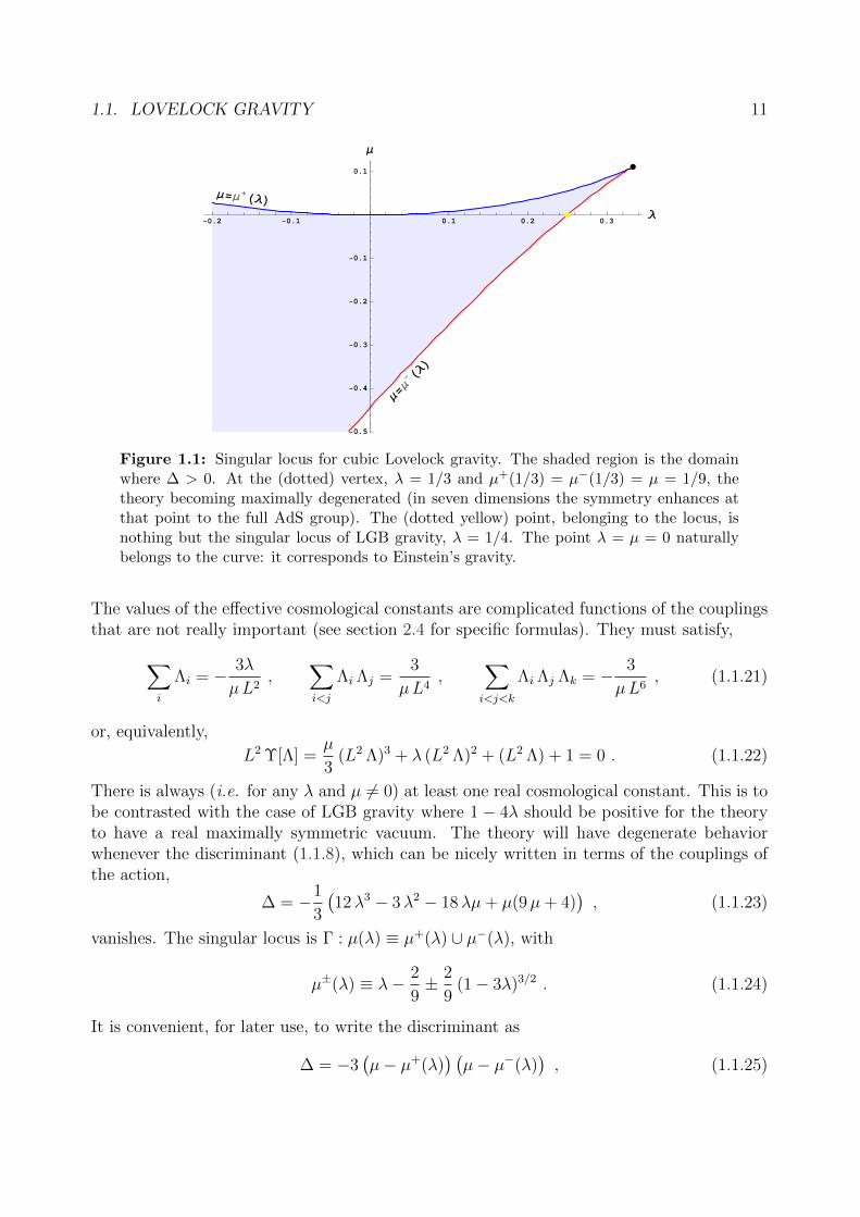
Figure 1.1: Singular locus for cubic Lovelock gravity. The shaded region is the domainwhere ∆ > 0. At the (dotted) vertex, λ = 1/3 and µ+(1/3) = µ−(1/3) = µ = 1/9, thetheory becoming maximally degenerated (in seven dimensions the symmetry enhances atthat point to the full AdS group). The (dotted yellow) point, belonging to the locus, isnothing but the singular locus of LGB gravity, λ = 1/4. The point λ = µ = 0 naturallybelongs to the curve: it corresponds to Einstein’s gravity.
The values of the effective cosmological constants are complicated functions of the couplingsthat are not really important (see section 2.4 for specific formulas). They must satisfy,∑
i
Λi = − 3λ
µL2,
∑i<j
Λi Λj =3
µL4,
∑i<j<k
Λi Λj Λk = − 3
µL6, (1.1.21)
or, equivalently,
L2 Υ[Λ] =µ
3(L2 Λ)3 + λ (L2 Λ)2 + (L2 Λ) + 1 = 0 . (1.1.22)
There is always (i.e. for any λ and µ 6= 0) at least one real cosmological constant. This is tobe contrasted with the case of LGB gravity where 1 − 4λ should be positive for the theoryto have a real maximally symmetric vacuum. The theory will have degenerate behaviorwhenever the discriminant (1.1.8), which can be nicely written in terms of the couplings ofthe action,
∆ = −1
3
(12λ3 − 3λ2 − 18λµ+ µ(9µ+ 4)
), (1.1.23)
vanishes. The singular locus is Γ : µ(λ) ≡ µ+(λ) ∪ µ−(λ), with
µ±(λ) ≡ λ− 2
9± 2
9(1− 3λ)3/2 . (1.1.24)
It is convenient, for later use, to write the discriminant as
∆ = −3(µ− µ+(λ)
) (µ− µ−(λ)
), (1.1.25)
12 CHAPTER 1. LOVELOCK THEORIES OF GRAVITY
since it makes clear that ∆ < 0 if µ > µ+(λ) or µ < µ−(λ), ∆ = 0 if µ = µ+(λ) orµ = µ−(λ), and ∆ > 0, elsewhere. We will see in what follows that the singular locus Γplays an important role. Notice that it does not depend in the spacetime dimensionality (ford ≥ 7). A similar analysis can be readily performed for higher-order Lovelock theories.
1.2 Gauss-Bonnet theorem and boundary terms
The action (1.0.4) defines a variational principle from which the equations of motion ofgeneral relativity can be derived. However, in the event that the manifold has a boundary,the action should be supplemented by a boundary term so that this variational principle iswell defined. This can be understood by means of a simple 1-dimensional example.
Consider the free particle lagrangian4
I =1
2
∫ t2
t1
x2dt . (1.2.1)
This action principle is designed in order to fix the position x at initial and final times, t1,2,i.e. δx(t1,2) = 0. Indeed,
δI =
∫ t2
t1
xδx dt =
∫ t2
t1
[−xδx+ ∂t(xδx)] dt (1.2.2)
=
∫ t2
t1
(−x)δx dt+ x(t2)δx(t2)− x(t1)δx(t1) .
Therefore for a solution of the equations, x = 0, of motion the action is minimal, δI = 0.We could equivalently have started off with a different action,
I ′ = −1
2
∫ t2
t1
xxdt , (1.2.3)
yielding the same equations of motion. This action principle is analogous to EH in the sensethat it is linear on second derivatives of x. In the same way as for EH, it is not possible tofix just x at the borders. In this case we get
δI ′ =
∫ t2
t1
(−x)δx dt (1.2.4)
− 1
2x(t2)δx(t2) +
1
2x(t1)δx(t1) +
1
2x(t2)δx(t2)− 1
2x(t1)δx(t1) .
Obviously, fixing x at t1,2 is not enough for solutions of the equations of motion to minimizethe action. We need to add a boundary term, the analogue of Gibbons-Hawking term inorder to fix the metric in GR. In this case it is easy to identify the missing term. The secondaction is related to the first by integration by parts, the difference being
1
2(x(t2)x(t2)− x(t1)x(t1)) . (1.2.5)
4We thank Andres Gomberoff for pointing this very pedagogical example to us.
1.2. GAUSS-BONNET THEOREM AND BOUNDARY TERMS 13
The variation of this term cancels the first two terms in (1.2.4) and adds up to the othertwo such that we get the original result (1.2.2). Again the action with the boundary term isobviously devised to fix x at the boundaries, it is exactly the original action. Although trivialin this context, conceptually the same happens with the EH action. We need to supplementit with the Gibbons-Hawking term so that the variational principle is well defined. Thedifference is that in the context of gravity we do not have available an analogue of the action(1.2.1).
The same logic carries over to any gravity theory and in particular to the Lovelock class.The need for boundary terms can be seen explicitly from the variation of the action withrespect to the spin connection (1.1.4). The first (boundary) term in the right hand side isanalogous to the unwanted terms in (1.2.4). Even though these terms do not change theequations of motion, they contribute to the variation of the action in such a way that thelatter is not minimized for solutions. We want to fix just the metric on the boundary, δea = 0,not its normal derivative, δωab 6= 0. Thus in order to cancel this boundary contribution wemust add a boundary term analogous to the Gibbons-Hawking term of GR [46,47],
IGH = ± 1
8πGN
∫∂Mdd−1x
ñhK , (1.2.6)
where hµν is the boundary metric and K = Kµµ the trace of the extrinsic curvature, the plus
(minus) sign applying to a spacelike (timelike) boundary.The well-posedness of the variational problem in the context of Lovelock gravity was
first analyzed in [48] and the explicit expression for the boundary terms was found. In thesame way as the kth Lovelock term is the dimensional continuation of the 2k-dimensionalEuler characteristic for closed manifolds, the corresponding boundary terms appear in thegeneralization of the Gauss-Bonnet theorem to manifolds with boundaries. For completenesswe give account of some basic formulæ connected to the Gauss-Bonnet theorem below. Webasically follow the discussion of [12].
The Euler number or Euler-Poincare characteristic, χ(M), is a topological invariant ofany manifold M on even dimensions, being zero if the dimension is odd. It is preservedunder homeomorphisms, i.e. one-to-one maps from one manifold to another in such a waythat the topology is preserved. For instance, a coffee cup and a doughnut share the sameEuler number, χ = 0. In general the Euler number is related to the genus, g, of the manifold,the number of handles on it, as
χ = 2− 2g . (1.2.7)
The Gauss-Bonnet theorem [11] allows to calculate the Euler number of a manifold ofdimension 2k as the integral of a density constructed solely from the curvature 2-form. Itcan be written as
χ(M) =(−1)k
(4π) k!
∫Mε(R, . . . R) . (1.2.8)
A very important property of the function function L(ω) = ε(Rk) is that under a continuouschange of the connection, ω → ω′, L(ω) changes by an exact form. This can be easily seenas follows. We omit indices for simplicity and define an interpolating connection
ωt = tω + (1− t)ω′ , (1.2.9)
14 CHAPTER 1. LOVELOCK THEORIES OF GRAVITY
calling
θ =d
dtωt = ω − ω′ . (1.2.10)
We also define the curvature associated with this new connection,
Rt = dωt + ωt ∧ ωt , (1.2.11)
and notice thatd
dtRt = Dtθ , (1.2.12)
where Dt is the covariant derivative associated with ωt. Then, we may write the variationof the Euler density as
ε(R, . . . R)− ε(R′, . . . R′) =
∫ 1
0
dtd
dtε(Rt, . . . Rt) = k
∫ 1
0
ε
(d
dtRt, Rt, . . . Rt
)= k
∫ 1
0
ε(Dtθ, Rt, . . . Rt) = k
∫ 1
0
dε(θ, Rt, . . . Rt) , (1.2.13)
where symmetry and linearity of ε(. . .) has been used, as well as the Bianchi identity, DtRt =0. If we define
Q(ω, ω′) = k
∫ 1
0
dt ε(ω − ω′, Rt, . . . Rt) , (1.2.14)
thenL(ω) = L(ω′) + dQ(ω, ω′) , (1.2.15)
in such a way that, in case the manifold M is compact (or non-compact, θ vanishing fastenough asymptotically), ∫
ML(ω) (1.2.16)
does not depend on ω, and obviously does not depend on the vielbein. Hence, the integralabove is a topological invariant as implied by the Gauss-Bonnet theorem. In the case of amanifold with boundary, ∂M, we can slightly modify the argument very easily in order toconstruct another invariant quantity. We may introduce a third (reference) connection, ω0,in such a way that
L(ω)− L(ω′) = [L(ω)− L(ω0)]− [L(ω′)− L(ω0)] = dQ(ω, ω0)− dQ(ω′, ω0) (1.2.17)
and we have demonstrated
L(ω)− dQ(ω, ω0) = L(ω′)− dQ(ω′, ω0) (1.2.18)
Therefore the new quantity ∫ML(ω)−
∫∂MQ(ω, ω0) (1.2.19)
is invariant under a continuous change of connection. This is a poor man’s way to show thatthe Euler class is a topological invariant, the real work is to prove that the actual value ofthe integral is related to χ.
1.2. GAUSS-BONNET THEOREM AND BOUNDARY TERMS 15
For vanishing torsion the above properties carry on trivially to any of the Lovelock terms.Once the corresponding boundary terms have been added, the variation of the full actionwith respect to the spin connection is exactly zero without any boundary contribution. Thevariation of the generalized Gibbons-Hawking term with respect to ω cancels the unwantedterm coming from the bulk action, and the variational problem is thus well posed. Thereference connection, ω0, is chosen to depend on the boundary metric, therefore it is keptfixed when extracting the equations.
In fact, even though the above argument is independent of ω0, this reference connectionis usually taken to be the spin connection for a product metric that agrees with the originalone on the boundary. In particular if we choose a set of adapted coordinates such that theboundary is y = 0, ω0 would be the connection associated with the metric
ds20 = n2dy2 + ds2
y=0 , (1.2.20)
where na is the unit normal vector to the boundary. It is clear that all the componentsaligned along the normal direction of this intrinsic spin connection are zero in the same wayas it happens for the corresponding intrinsic curvature,
R0 = dω0 + ω0 ∧ ω0 . (1.2.21)
In this way, the spin connection difference with respect to this reference metric,
θ = ω − ω0 , (1.2.22)
has a very neat geometric interpretation, becoming the second fundamental form of theboundary surface. As we will explain below, the second fundamental form is related to theextrinsic curvature of the surface and it is zero for purely boundary components.
The boundary terms appearing in the Gauss-Bonnet theorem, once dimensionally con-tinued, are the natural generalization of the Gibbons-Hawking term. The latter correspondsto the simplest k = 1 case that can also be written as
Q1 = θa1a2 ∧ ea3···ad εa1···ad , (1.2.23)
in terms of differential forms, and the analogous term in LGB gravity, so-called Myers term[48],
Q2 = 2θa1a2 ∧ (Ra3a4 − 2
3θa3
c ∧ θca4) ∧ ea5···ad εa1···ad . (1.2.24)
For the reasons outlined above, any general Lovelock action (1.1.1), defined by a setcoupling constants ck, has to be supplemented by a boundary term
I∂ =K∑k=1
ckd− 2k
∫∂MQk , (1.2.25)
the individual boundary densities being simply,
Qk = k
∫ 1
0
dξ εa1···ad θa1a2 ∧Ra3a4
ξ ∧ . . . ∧Ra2k−1a2k
ξ ea2k+1···ad , (1.2.26)
16 CHAPTER 1. LOVELOCK THEORIES OF GRAVITY
whereRabξ = ξRab + (1− ξ)Rab
0 − ξ(1− ξ)(θ ∧ θ)ab . (1.2.27)
We have omitted the overall normalization factor 1/16πGN(d − 3)!. The total action is in
this way I = I −I∂ and can be written as a sum of dimensionally continued Euler densities.In order to get simplified expressions involving just the curvature R and θ in the spirit
of (1.2.24) we may make use of
Rab = Rab0 +D0θ
ab + (θ ∧ θ)ab (1.2.28)
and also take into account that D0θab = dθab + (ω0 ∧ θ)ab + (θ ∧ ω0)ab is zero unless either
one of the indices is in the normal direction. As the whole expression is multiplied by thesecond fundamental form that necessarily picks one index in the normal direction in ordernot to vanish, this term does not contribute to (1.2.26) and we can write it in terms of justthe full curvature and the second fundamental form as
Qk = k
∫ 1
0
dξ θa1a2 ∧Ra3a4(ξ) ∧ . . . ∧Ra2k−1a2k(ξ) ∧ ea2k+1···adεa1···ad , (1.2.29)
where Rab = Rab + (ξ2 − 1)(θ ∧ θ)ab. The Gibbons-Hawking and Myers terms as writtenabove are the individual contributions for k = 1, 2.
Sometimes it is more natural and useful to write (1.2.29) in terms of the extrinsic andintrinsic curvatures of the boundary. In chapter 5 we will make extensive use of this form ofthe boundary terms. The extrinsic curvature is related to the second fundamental form as
θab = n2(naKb − nbKa) , (1.2.30)
where again na is the normal vector to the surface and KA = KABe
B is the extrinsiccurvature 1-form. The extrinsic curvature can in turn be calculated as covariant derivativeof the normal vector as
KAB = eµA∇eBnµ = −nµ∇eBeµA , (1.2.31)
where we used the fact that na is normal to the vielbein basis induced on the surface. Takinginto account (1.2.30) and
θab ∧ θbc = −n2Ka ∧Kc (1.2.32)
we finally get
Qk = −2k
∫ 1
0
dξ KA1 ∧RA2A30 (ξ) ∧ . . . ∧R
A2k−2A2k−1
0 (ξ) eA2k···Ad−1εA1···Ad−1, (1.2.33)
where RAB0 = RAB
0 − ξ2 n2KA ∧ KB and everything has been expressed in terms of thevielbein basis adapted to the surface such that
naεab... ∼ −n2εB... (1.2.34)
This will be consistent with our conventions in chapter 5.Another important role of the boundary terms in general relativity is that they give
rise to the so-called Israel junction conditions that govern the dynamics of shells separating
1.2. GAUSS-BONNET THEOREM AND BOUNDARY TERMS 17
different bulk domains [49] By performing an integration of Einstein’s equations across theshell and taking the thickless limit it is possible to show that the jump in the extrinsiccurvature is related to the surface stress-energy tensor, SAB,
K+AB −K
−AB = 8πGN
(SAB −
1
2ηABS
). (1.2.35)
It can be shown that Israel’s method for singular hypersurfaces is equivalent to an actionprinciple with boundary terms at the hypersurface, the variation of the latter yielding thejunction conditions [50].
The Lovelock action in the presence of singular hypersurfaces can also be written interms of smooth bulk integrals plus boundary terms [51–53], that in the case of n = 2 LGBtheory was first written down by Davis [54]. One may consider the spacetime manifold asthe union of two submanifolds with a common boundary Σ in such a way that in additionto the boundary term at infinity we get two extra surface terms at the boundary betweenthe two. The action in this case would be written as
Itot = (I− − I−∂ ) + (I+ + I+∂ )− I∂ , (1.2.36)
where − (+) denote the inner (outer) region. Remark that the form of the surface terms atΣ is the same as that of the boundary term at infinity,
IΣ = −I−∂ + I+∂ , (1.2.37)
the plus sign in the second term coming from the fact that the bulk regions induce oppositeorientations on the common boundary5. In case the spin connection is continuous at Σ, IΣ
vanishes and we recover the usual Lovelock action.This way of writing the action is useful in order to find solutions where the spin connection
is discontinuous across some codimension one hypersurface (the metric being continuous).The variation of the bulk terms on each side yield the usual Lovelock equations of motionwhile the junction conditions arise from the variation of the boundary terms with respect tothe induced vielbein field or equivalently the pullback of the metric on Σ. We will commentmore on this in section 5 where we will be interested in this kind of distributional solutions.The issue of finding equations with singular sources is a non-trivial one in non-linear gravitytheories as many operations with distributions are not unambiguously defined.
In order to take the variation of the action written in this way we also have to vary withrespect to the spin connection induced in the intermediate surface. This variation is againzero as it cancels the boundary term coming from the bulk integrals (this is the reason weintroduced these terms to begin with) whereas the variation with respect to the intrinsicmetric is proportional to the canonical momenta in such a way that the variation of eachterm may be written as
δI∂ = −∫∂M
dd−1x πABδhAB . (1.2.38)
5One can also construct solutions with the same orientation on both sides leading in turn to wormholesand Randrall-Sundrum-like models [55,56]
18 CHAPTER 1. LOVELOCK THEORIES OF GRAVITY
Therefore, the junction conditions at the surface Σ amount precisely to continuity of thecanonical momenta [57–59]. The analogous term from the boundary does not contribute aswe keep the boundary metric fixed, δh = 0. The canonical momenta in Lovelock gravity canbe expressed as
πBC = −1
2
δI∂δeC∧ eB (1.2.39)
=K∑k=1
k ck
∫ 1
0
dξ KA1 ∧RA2A30 (ξ) ∧ . . . ∧R
A2k−2A2k−1
0 (ξ) eA2k···Ad−2BεA1···Ad−2C ,
The generalization of the Israel junction conditions to Lovelock gravity being
π+AB − π
−AB = 8πGN SAB (1.2.40)
that reduces to (1.2.35) in the case of EH gravity.Junction conditions can also be seen to arise in our 1-dimensional example. First of all,
the same kind of boundary term appears if we split the action, or the interval of integration,in two. The variation of each term in that case is
δI− =
∫ t?
t1
dt
[∂L
∂q− d
dt
(∂L
∂q
)]δq +
∂L
∂q
∣∣∣∣t?
δq? (1.2.41)
The first term vanishes because of the equations of motion but the second does not as theposition is not fixed for t = t?. That term combines from an analogous one coming from theother part of the action, I+, to yield the junction condition
p− − p+ = 0 , (1.2.42)
i.e. continuity of the canonical momentum. For univalued momentum such as in (1.2.1)this in turn implies the continuity of the velocity. The free particle trajectory is necessarilycontinuous and smooth without any need of imposing any of these conditions a priori. Thereis no non-smooth solution of x = 0. In the same way as for EH gravity, in order to add adiscontinuity in the velocity we need to include new source terms. In the particle examplethe analogue of a dust shell would be localized at a given time, t = 0 for simplicity.
I = I +
∫ t2
t1
dtλxδ(t) = I + λx(0) . (1.2.43)
When varying the action, fixing x in the borders, x(t1,2) = x1,2 we get the equation
d
dt
(∂L
∂x
)− ∂L
∂x= λδ(t) . (1.2.44)
This equation includes junction conditions that can be found by integrating in infinitesimalregion around t = 0, between t = 0− and t = 0+. In this way we find
p+ − p− = λ , (1.2.45)
1.2. GAUSS-BONNET THEOREM AND BOUNDARY TERMS 19
where p± = p(0±). We could also have started with the splitted action in which case thejunction conditions would arise from the variation on the shell, in this case the variation ofx(0) which is not fixed by the boundary conditions.
In order to keep the discussion as general as possible we will consider the action writtenin terms of the canonical variables q and p instead of the velocity,
L(q, p) = pq −H(q, p) . (1.2.46)
In this way the lagrangian can be varied independently with respect to the two canonicalvariables, q and p, yielding the well known Hamilton equations,
p = −∂H∂q
; q =∂H
∂p. (1.2.47)
In the same way as before this action is prepared to fix the value of the position at theextrema, δq = 0. However we can also use a different lagrangian,
L′(q, p) = −pq −H(q, p) , (1.2.48)
that in turn is prepared to fix the momenta p instead. This can be easily understood as aresult of the transformation q ↔ p, q ↔ −p between the two lagrangians. However we cansupplement the latter (1.2.48) with a boundary term in such a way that it is equivalent to(1.2.46),
L(q, p) = L′(q, p) +d
dt(pq) (1.2.49)
Obviously the right hand side is obtained from the original lagrangian just by integrating byparts. The nice thing about this way of writing the action is that now we can split a giveninterval in two pieces and vary the action not just with respect to the bulk variables but alsowith respect to the ones at the shell, t = t?,
I ′ =
∫ t?
t1
dt L′(q, p) + (p− − p+)q? +
∫ t2
t?dt L′(q, p) . (1.2.50)
The variation with respect to the momentum on the shell again cancels the contribution ofthe boundary term, whereas inside the intervals (t1, t?) and (t?, t2) it also vanishes due to theequations of motion. The only contribution to the variation thus comes from the variationof the boundary term with respect to the shell position,
δI ′ = (p− − p+)δq? , (1.2.51)
again implying the continuity of the canonical momentum across the discontinuity. We mayalso add source terms that induce jumps in the canonical momentum, similar to singularmatter distributions in GR.
As we mentioned above, for univalued momentum, its continuity implies that the thevelocity is continuous as well. In more general cases however, the momentum may be multi-valued this becoming a non-trivial equation. The velocity may jump as long as the canonicalmomentum is conserved. We will comment more on this on chapter 5, with a specific exam-ple.
20 CHAPTER 1. LOVELOCK THEORIES OF GRAVITY
Chapter 2
Lovelock black holes
“To myself I am only a child playing on the beach,while vast oceans of truth lie undiscovered before me.”
Isaac Newton
The concept of singularity is central to general relativity. Due to the attractive and uni-versal nature of the gravitational interaction, the theory predicts that these kind of objectsinevitably form, either in the form of a black hole or as a cosmological singularity such asthe Big Bang.
The first to describe a singular solution of the equations of general relativity was KarlSchwarzschild [60] already in 1916, soon after the publication of Einstein’s original paper.It was the first exact solution of Einstein’s equations besides the trivial Minkowski metric.Unfortunately, Schwarzschild had contracted a disease while serving in the German armyduring World War I and died shortly after his paper was published. The singular characterof the solution he found was at first considered just as a mathematical curiosity, of nonephysical relevance, until it was realized quite a long time afterwards that such objects actuallydo generally form from the collapse of matter [61, 62] such as that of a dying star. Thedensity of a physical object of radius R is bounded, in such a way that if R dips below theSchwarzschild radius the system will undergo gravitational collapse and become a black hole.However it was not until the sixties, with the advent of the singularity theorems of Hawkingand Penrose [63, 64], that the debate was definitely settled. In short, a black hole is a self-gravitating object so densely packed that nothing, not even light, can scape its gravitationalattraction. Nowadays black holes are thought to be quite common objects in the Universebeing generally present at the center of galaxies such as the Milky Way. They cannot bedirectly seen but their presence is detected through the trajectories of stars on their vicinityor radiation coming from their accretion disks.
21
22 CHAPTER 2. LOVELOCK BLACK HOLES
The fact that the gravitational field can affect the trajectory of light rays is well known.In fact it was the way Eddington proved Einstein theory right in his famous 1919 expeditionto Africa. The idea of an object from which not even light can scape is much older though.We can trace it back as far as 1783, to a letter [65] John Michell sent to Henry Cavendish, hisfellow at the Royal Society of London. In that letter, using just Newtonian gravity, Michelldescribes the hypothetical case of a heavenly object so massive that not even light couldescape its gravitational pull. Michell speculated, were the escape velocity at the surface ofa star equal or greater than the speed of light, the generated light would be gravitationallytrapped, and the star invisible to a distant observer. He named his discovery dark star, theprecursor of black holes.
For an object leaving the surface of a dark star of mass M with some speed v ≥ vs toreach infinity we need the sum of its kinetic and gravitational energy to be equal or greaterthan zero,
1
2mv2 − GNMm
R≥ 0 ⇒ v2
s =2MGN
R(2.0.1)
in such a way that the radius of the dark star has to be smaller than
R ≤ RS ≡2MGN
c2(2.0.2)
which, curiously enough, is independent of the mass of the object and actually coincides withthe Schwarzschild radius of general relativity, r = 2M in geometric units. In that contextthis particular radial position is named event horizon.
The concept of black hole is quite different from that of a dark star. Nothing sent fromthe dark star can reach infinity but it can leave the star and even reach infinity if we furnishsome extra acceleration. The black hole however is provided with an event horizon that actsas a one way membrane. Objects can get into the horizon but they cannot get back out.More precisely, consider the form of the Schwarzschild metric in general relativity
ds2 = −(
1− 2M
r
)dt2 +
dr2(1− 2M
r
) + r2dΩ2 . (2.0.3)
The time and radial variables exchange their roles beyond r = 2M in such a way that ther coordinate becomes timelike and t spacelike. Being timelike, r has to decrease along anytimelike trajectory in the same way as the time ticks forward outside the black hole. In fact,any object falling through the event horizon will reach the central singularity in finite propertime, it would be inevitably driven there.
The event horizon plays yet another very important role. As it prevents anything fromleaving the black hole, it effectively divides the spacetime in two. Nothing happening insidethe horizon can ever influence the dynamics of the exterior region. This is essential in orderto have a well-defined initial value problem in the presence of a singularity. The singularityrepresents a break down of the theory, in a sense, it is the place where general relativity showsits failure. It is also the place where quantum effects become dramatically important so thatwe would need a quantum theory of gravity to disclose the dynamics at the singularity. Theexistence of the event horizon protects the exterior region from this unknown dynamics, theexterior evolution being always well defined. In 1969 Penrose made this idea precise and
2.1. BLACK HOLES IN LOVELOCK GRAVITY 23
conjectured that, in the context of general relativity, there can be no singularity visible fromfuture null infinity. In other words, singularities need to be hidden from any observer atinfinity by the event horizon of a black hole. This is known as the weak cosmic censorshiphypothesis [66].
We will study the analogous solution to that of Schwarzschild in the context of generalLovelock theories of gravity. Finding an analytic black hole solution requires to explicitlysolve a polynomial equation and we are certainly restricted by the implications of Galoistheory; meaningly, quartic is the highest order polynomial equation that can be genericallysolved by radicals (Abel-Ruffini theorem). However, an implicit but exact solution can befound, and we develop some tools to extract all relevant information, mainly their horizonstructure and thermodynamics. We will devote this chapter to present our proposal to dealwith generic black holes in Lovelock theory, focusing in the case of LGB and cubic Lovelockfor a detailed description. In the next chapter we perform a classification of all possible blackhole solutions, including the case of asymptotically dS solutions, and all possible horizontopologies within maximally symmetric configurations.
The analysis of these solutions for the Lovelock family may also provide some usefulinformation about the dynamics of black holes in more general gravity theories. This is spe-cially important due to the high nonlinearity of the field equations that makes very difficultfinding nontrivial analytical solutions of Einstein’s equation with higher derivative terms. Inmost cases, one has to adopt some approximation methods or find solutions numerically. Inthe last few months there were some papers constructing gravitational theories that sharesome compelling properties with Lovelock lagrangians [67,68]. In particular, these are lowerdimensional theories displaying black hole solutions whose profile precisely correspond toLovelock black holes [69, 70]. In particular these theories allow for the addition of an extraterm of degree K = d+1
2in odd dimensions [70], contributing in every way as the correspond-
ing Lovelock term in higher dimensions. Some other higher order terms may be also addedthat do not change the form of the black hole solution. Some of the results of this thesisare therefore of direct application to those cases as well. This is particularly interesting dueto the fact that quasi-topological gravities are higher curvature theories in dimensions lowerthan their corresponding Lovelock cousins, thus the results are of interest in more ‘physical’setups of AdS/CFT [71].
2.1 Black holes in Lovelock gravity
It has been shown in [72] that Lovelock theories admit asymptotically (A)dS solutions withnon-trivial horizon topologies. We can consider for instance solutions with a planar orhyperbolic symmetry as a straightforward generalization of the usual spherically symmetricansatz,
ds2 = −A(t, r) dt2 +dr2
B(t, r)+r2
L2dΣ2
d−2,σ , (2.1.1)
where
dΣ2d−2,σ =
dρ2
1− σρ2/L2+ ρ2dΩ2
d−3 , (2.1.2)
24 CHAPTER 2. LOVELOCK BLACK HOLES
is the metric of a (d−2)-dimensional manifold of negative, zero or positive constant curvature(σ = −1, 0, 1 parametrizing the different horizon topologies), and dΩ2
d−3 is the metric of theunit (d− 3)-sphere. This does not imply that the horizon is just spherical or non-compact.By means of the Killing-Hopf theorem [73], any complete connected Riemannian manifold ofEuclidean signature and constant curvature σ can be written as a quotient space Σd−2,σ/Γ,where Γ is a discrete subgroup of the isometry group of Σd−2,σ. Thus, even in (what we shallcall) the spherical case, we have non-spherical possibilities; for example, one may take thehorizon to be a lens space. Besides, planar or hyperbolic horizons can be made compact inthis way.
It has been proven in [74] that these black holes admit a version of Birkhoff’s theorem,in such a way that in addition to the SO(d−1), Ed−2 or SO(1, d−2) isometry groups, thesespacetimes admit an extra timelike killing vector (for A,B > 0). This means that these so-lutions of the field equations are locally isometric to their corresponding static counterparts,which can be found by means of the ansatz
ds2 = −f(r) dt2 +dr2
f(r)+r2
L2dΣ2
d−2,σ . (2.1.3)
There are extra solutions with different functions in the timelike and radial direction butthey are just valid for degenerate values of the cosmological constant [75]. In that case, themost general solution is
ds2 = −f(r) dt2 +dr2
(σ − Λ r2)+r2
L2dΣ2
d−2,σ , (2.1.4)
for any function f(r). This allows in particular Lifshitz-like solutions f(r) ∼ r2z for anyvalue of the critical exponent z.
These black hole solutions are all three asymptotic to a maximally symmetric space.Thus, when considering the same curvature for all of them they are locally asymptoticallyequivalent, but globally different. They are often referred to as topological black holes forthis reason. Indeed, there are global changes of coordinates that relate the sets of coordinatescorresponding to the three topologically different vacuum solutions associated with a givenΛ [76]. Each set covers a different patch of AdS and has a different time coordinate. Thus, wecan also look at the different topologies as static black holes for different classes of observers.
Using the natural frame,
e0 =√f(r) dt , e1 =
1√f(r)
dr , ea =r
Lea , (2.1.5)
where a = 2, . . . , d− 1, and Rab = σ ea ∧ eb. The Riemann 2-form reads
R01 = −1
2f ′′(r) e0 ∧ e1 , R0a = −f
′(r)
2re0 ∧ ea ,
R1a = −f′(r)
2re1 ∧ ea , Rab = −f(r)− σ
r2ea ∧ eb . (2.1.6)
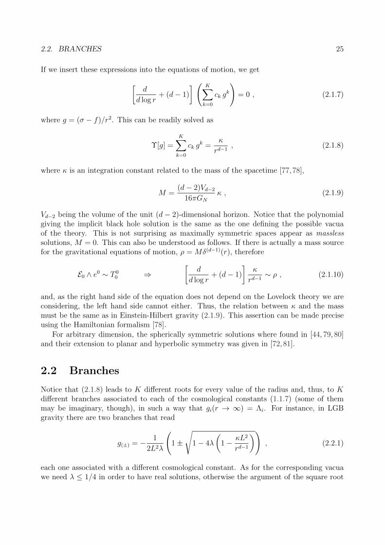
2.2. BRANCHES 25
If we insert these expressions into the equations of motion, we get[d
d log r+ (d− 1)
] ( K∑k=0
ck gk
)= 0 , (2.1.7)
where g = (σ − f)/r2. This can be readily solved as
Υ[g] =K∑k=0
ck gk =
κ
rd−1, (2.1.8)
where κ is an integration constant related to the mass of the spacetime [77,78],
M =(d− 2)Vd−2
16πGN
κ , (2.1.9)
Vd−2 being the volume of the unit (d− 2)-dimensional horizon. Notice that the polynomialgiving the implicit black hole solution is the same as the one defining the possible vacuaof the theory. This is not surprising as maximally symmetric spaces appear as masslesssolutions, M = 0. This can also be understood as follows. If there is actually a mass sourcefor the gravitational equations of motion, ρ = Mδ(d−1)(r), therefore
E0 ∧ e0 ∼ T 00 ⇒
[d
d log r+ (d− 1)
]κ
rd−1∼ ρ , (2.1.10)
and, as the right hand side of the equation does not depend on the Lovelock theory we areconsidering, the left hand side cannot either. Thus, the relation between κ and the massmust be the same as in Einstein-Hilbert gravity (2.1.9). This assertion can be made preciseusing the Hamiltonian formalism [78].
For arbitrary dimension, the spherically symmetric solutions where found in [44, 79, 80]and their extension to planar and hyperbolic symmetry was given in [72,81].
2.2 Branches
Notice that (2.1.8) leads to K different roots for every value of the radius and, thus, to Kdifferent branches associated to each of the cosmological constants (1.1.7) (some of themmay be imaginary, though), in such a way that gi(r → ∞) = Λi. For instance, in LGBgravity there are two branches that read
g(±) = − 1
2L2λ
(1±
√1− 4λ
(1− κL2
rd−1
)), (2.2.1)
each one associated with a different cosmological constant. As for the corresponding vacuawe need λ ≤ 1/4 in order to have real solutions, otherwise the argument of the square root
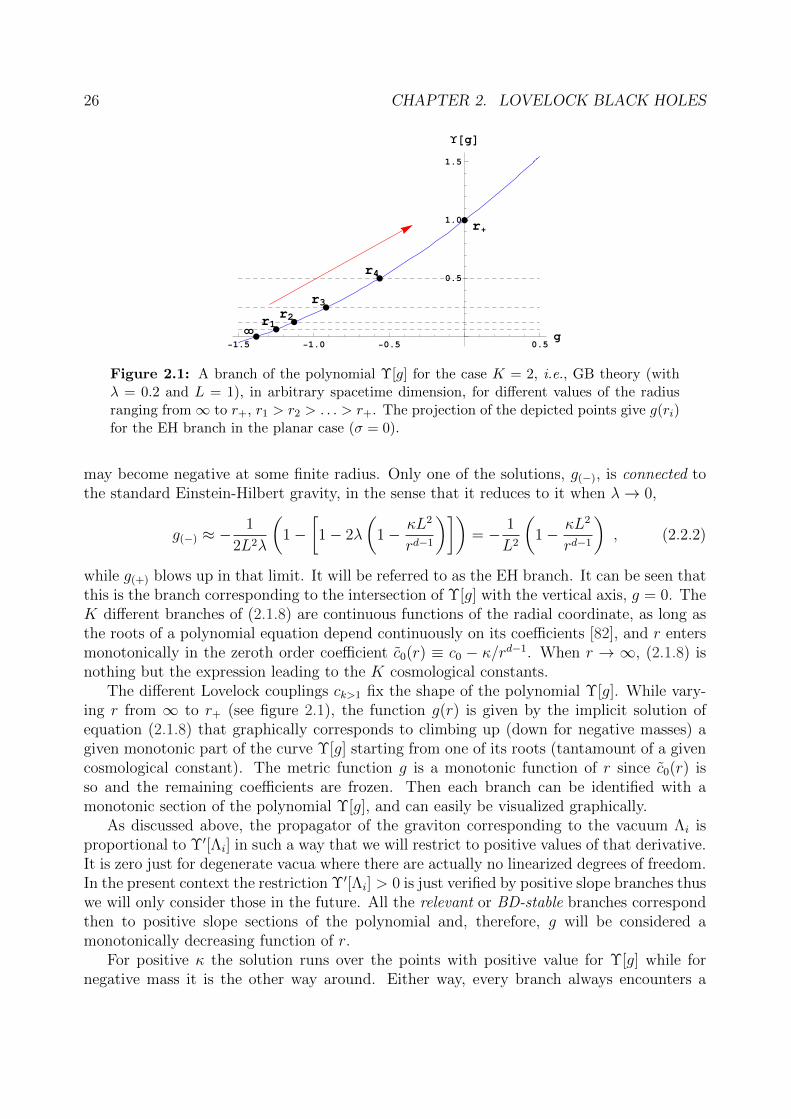
26 CHAPTER 2. LOVELOCK BLACK HOLES
-1.5 -1.0 -0.5 0.5g
0.5
1.0
1.5
U@gD
¥
r+
r4
r3r2r1
Figure 2.1: A branch of the polynomial Υ[g] for the case K = 2, i.e., GB theory (withλ = 0.2 and L = 1), in arbitrary spacetime dimension, for different values of the radiusranging from∞ to r+, r1 > r2 > . . . > r+. The projection of the depicted points give g(ri)for the EH branch in the planar case (σ = 0).
may become negative at some finite radius. Only one of the solutions, g(−), is connected tothe standard Einstein-Hilbert gravity, in the sense that it reduces to it when λ→ 0,
g(−) ≈ −1
2L2λ
(1−
[1− 2λ
(1− κL2
rd−1
)])= − 1
L2
(1− κL2
rd−1
), (2.2.2)
while g(+) blows up in that limit. It will be referred to as the EH branch. It can be seen thatthis is the branch corresponding to the intersection of Υ[g] with the vertical axis, g = 0. TheK different branches of (2.1.8) are continuous functions of the radial coordinate, as long asthe roots of a polynomial equation depend continuously on its coefficients [82], and r entersmonotonically in the zeroth order coefficient c0(r) ≡ c0 − κ/rd−1. When r → ∞, (2.1.8) isnothing but the expression leading to the K cosmological constants.
The different Lovelock couplings ck>1 fix the shape of the polynomial Υ[g]. While vary-ing r from ∞ to r+ (see figure 2.1), the function g(r) is given by the implicit solution ofequation (2.1.8) that graphically corresponds to climbing up (down for negative masses) agiven monotonic part of the curve Υ[g] starting from one of its roots (tantamount of a givencosmological constant). The metric function g is a monotonic function of r since c0(r) isso and the remaining coefficients are frozen. Then each branch can be identified with amonotonic section of the polynomial Υ[g], and can easily be visualized graphically.
As discussed above, the propagator of the graviton corresponding to the vacuum Λi isproportional to Υ′[Λi] in such a way that we will restrict to positive values of that derivative.It is zero just for degenerate vacua where there are actually no linearized degrees of freedom.In the present context the restriction Υ′[Λi] > 0 is just verified by positive slope branches thuswe will only consider those in the future. All the relevant or BD-stable branches correspondthen to positive slope sections of the polynomial and, therefore, g will be considered amonotonically decreasing function of r.
For positive κ the solution runs over the points with positive value for Υ[g] while fornegative mass it is the other way around. Either way, every branch always encounters a
2.3. SINGULARITIES AND HORIZONS 27
maximum/minimum, or it grows unboundedly.For the sake of clarity and the ease of reading, let us first classify the different types
of branches that one may encounter when dealing with a Lovelock theory of gravity. Theappearance of a given type of branch will depend, in general, on the specific theory consideredand on the values of the different coupling constants. On the one hand, we may classify thebranches by their asymptotics: AdS, flat or dS branches. In the particular case we areconsidering, with c0 = L−2, there are no asymptotically flat branches. The sign of thecosmological constant corresponding to the EH branch (when real) is the opposite to c0 (or,equivalently, the same as the explicit cosmological constant, as in standard Einstein-Hilbertgravity); thus, the EH branch is asymptotically AdS. Due to the particular features andrelevance of this branch, we will consider it separately.
Some of the branches (monotonic sections of the polynomial) may also be associatedto complex values of Λ. Therefore, they do not correspond to real metrics and should bedisregarded as unphysical. We will refer to these as excluded branches, and to the sector ofthe parameter space where the EH branch is excluded as the excluded region.
We will then exhaustively classify branches on (non-EH) AdS (i.e., not crossing g = 0),EH, dS and excluded branches. The latter, being unphysical, do not need further discussion.The AdS branches must end at a maximum of the polynomial in order not to cross g = 0.The other two cases may end at a maximum or, else, continue all the way up to g →∞. Wewill then consider two subclasses of branches: those (a) continuing all the way to infinity or(b) ending at a maximum. For the AdS branches we will also consider two subclasses: (a)positive mass and (b) negative mass.
2.3 Singularities and horizons
Where are the singularities of these spacetimes located? The simplest way to answer thisquestion is to calculate the curvature scalar and see where it diverges. As it depends on themetric and its derivatives, these divergences can be traced back to those of the first derivativeof g,
g′ = −(d− 1)κ
rdΥ′[g]−1 . (2.3.1)
Then, the metric is regular everywhere except at r = 0 and at points where Υ′[g] = 0; thatis, whenever the branch we are looking at coincides with any other. In such case,
Υ′[g] =K∑k=1
k ck gk−1 = 0 . (2.3.2)
These are precisely the maxima/minima at which all branches end, except those growingunboundedly (that also approach asymptotically to a singularity located at r = 0). Thevalues of r where this happens exhibit a curvature singularity that prevents from entering aregion where the metric becomes complex. Type (a) branches correspond to solutions witha singularity at r = 0 whereas those of (b) type display the singularity at finite radius.
It can be easily seen that the mass parameter κ must be positive in the planar case(σ = 0) in order for the spacetime to have a well-defined horizon. We can actually rewrite
28 CHAPTER 2. LOVELOCK BLACK HOLES
equation (2.1.8) asK∑k=1
ck gk =
κ
rd−1− 1
L2, (2.3.3)
and realize that the equation admits a vanishing g only when r = r+ ≡ (κL2)1d−1 . In the
planar case, furthermore, only one branch has a horizon at r+ and all the rest display nakedsingularities. This is so since the polynomial root g = 0 has multiplicity one at r = r+
(higher multiplicity would require a vanishing coefficient of the Einstein-Hilbert term). Inthe case of LGB theory, for instance, we can see from (2.2.1) that it is g(−). This is theabove mentioned EH branch, a deformation of the solution to pure Einstein-Hilbert theory,and the only branch that remains when turning all the extra couplings off. Since Υ′[0] > 0,g(r) in the EH branch is decreasing close to r+ and, thus, it is a relevant branch.
For non-planar horizons the situation is more complicated and, in principle, some of thebranches admit horizonful black hole solutions even for negative values of κ. The physicalmass of the black hole has to match the one of the matter contained in that region ofspacetime. Thus, κ will be considered a positive quantity, except for hyperbolic black holesfor which some comments on negative mass solutions shall be made. In [83], indeed, theformation by collapse of black holes with negative mass has been considered. We shall seethat spherical or planar black holes always exhibit a naked singularity in the case of negativemass. The only horizon that may arise for those solutions is a cosmological one. This is thecase for negative mass asymptotically dS branches even for hyperbolic topology.
Taking into account that the value of g at the event horizon, r = r+, reads
g+ ≡σ
r2+
, (2.3.4)
we can write κ = rd−1+ Υ[σ/r2
+]. The other way around, the radii of the location of thehorizons are given by solutions of the previous equation for any given value of κ. This leadsto a more handy formula for the mass
M =(d− 2)Vd−2
16πGN
rd−1+ Υ
[σ
r2+
]. (2.3.5)
Following the argument used to derive (2.1.10), and taking into account that Einstein-Hilbertgravity has a positive energy theorem, we are tempted to conjecture that the same shouldapply to any Lovelock theory though this has not been proven so far. This conjecturedpositivity would not in principle rule out the negative mass solutions mentioned before asit may happen that the positive mass corresponds to the difference of the mass previouslydefined with the extremal one [84].
We can recast the equation for the horizon, by means of (2.1.8) and (2.3.4), in such away that it can be plotted in the (g,Υ[g])-plane,
Υ[g+] = κ
(√g+
σ
)d−1
, (2.3.6)
where the right hand side is just defined for positive/negative values of g+, for σ = ±1,while for σ = 0 the expression is not strictly valid since, in that case, g+ exactly vanishes.
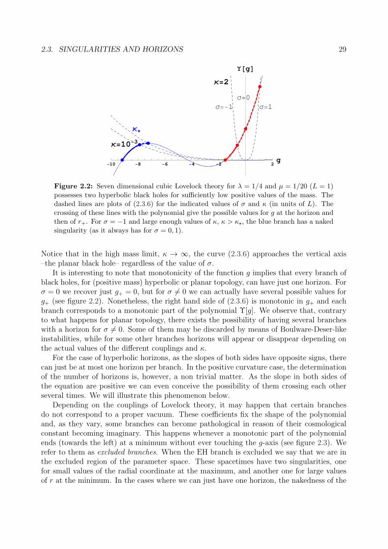
2.3. SINGULARITIES AND HORIZONS 29
-10 -8 -6 -4 -2 2g
U@gD
Κ*
Σ=1Σ=0
Σ=-1
Κ=2
Κ=10-3
Figure 2.2: Seven dimensional cubic Lovelock theory for λ = 1/4 and µ = 1/20 (L = 1)possesses two hyperbolic black holes for sufficiently low positive values of the mass. Thedashed lines are plots of (2.3.6) for the indicated values of σ and κ (in units of L). Thecrossing of these lines with the polynomial give the possible values for g at the horizon andthen of r+. For σ = −1 and large enough values of κ, κ > κ?, the blue branch has a nakedsingularity (as it always has for σ = 0, 1).
Notice that in the high mass limit, κ → ∞, the curve (2.3.6) approaches the vertical axis–the planar black hole– regardless of the value of σ.
It is interesting to note that monotonicity of the function g implies that every branch ofblack holes, for (positive mass) hyperbolic or planar topology, can have just one horizon. Forσ = 0 we recover just g+ = 0, but for σ 6= 0 we can actually have several possible values forg+ (see figure 2.2). Nonetheless, the right hand side of (2.3.6) is monotonic in g+ and eachbranch corresponds to a monotonic part of the polynomial Υ[g]. We observe that, contraryto what happens for planar topology, there exists the possibility of having several brancheswith a horizon for σ 6= 0. Some of them may be discarded by means of Boulware-Deser-likeinstabilities, while for some other branches horizons will appear or disappear depending onthe actual values of the different couplings and κ.
For the case of hyperbolic horizons, as the slopes of both sides have opposite signs, therecan just be at most one horizon per branch. In the positive curvature case, the determinationof the number of horizons is, however, a non trivial matter. As the slope in both sides ofthe equation are positive we can even conceive the possibility of them crossing each otherseveral times. We will illustrate this phenomenon below.
Depending on the couplings of Lovelock theory, it may happen that certain branchesdo not correspond to a proper vacuum. These coefficients fix the shape of the polynomialand, as they vary, some branches can become pathological in reason of their cosmologicalconstant becoming imaginary. This happens whenever a monotonic part of the polynomialends (towards the left) at a minimum without ever touching the g-axis (see figure 2.3). Werefer to them as excluded branches. When the EH branch is excluded we say that we are inthe excluded region of the parameter space. These spacetimes have two singularities, onefor small values of the radial coordinate at the maximum, and another one for large valuesof r at the minimum. In the cases where we can just have one horizon, the nakedness of the
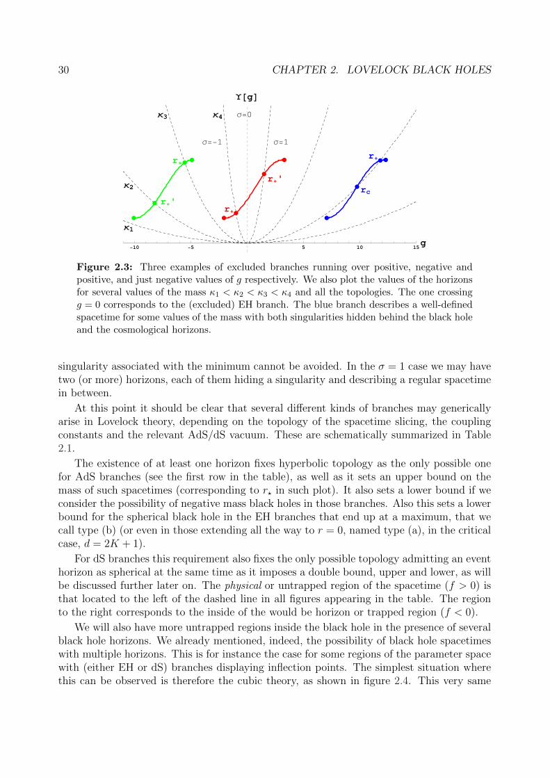
30 CHAPTER 2. LOVELOCK BLACK HOLES
-10 -5 5 10 15g
U@gD
Σ=1
Σ=0
Σ=-1
Κ1
Κ2
Κ3 Κ4
rc
r+
r+'
r+
r+
r+'
Figure 2.3: Three examples of excluded branches running over positive, negative andpositive, and just negative values of g respectively. We also plot the values of the horizonsfor several values of the mass κ1 < κ2 < κ3 < κ4 and all the topologies. The one crossingg = 0 corresponds to the (excluded) EH branch. The blue branch describes a well-definedspacetime for some values of the mass with both singularities hidden behind the black holeand the cosmological horizons.
singularity associated with the minimum cannot be avoided. In the σ = 1 case we may havetwo (or more) horizons, each of them hiding a singularity and describing a regular spacetimein between.
At this point it should be clear that several different kinds of branches may genericallyarise in Lovelock theory, depending on the topology of the spacetime slicing, the couplingconstants and the relevant AdS/dS vacuum. These are schematically summarized in Table2.1.
The existence of at least one horizon fixes hyperbolic topology as the only possible onefor AdS branches (see the first row in the table), as well as it sets an upper bound on themass of such spacetimes (corresponding to r? in such plot). It also sets a lower bound if weconsider the possibility of negative mass black holes in those branches. Also this sets a lowerbound for the spherical black hole in the EH branches that end up at a maximum, that wecall type (b) (or even in those extending all the way to r = 0, named type (a), in the criticalcase, d = 2K + 1).
For dS branches this requirement also fixes the only possible topology admitting an eventhorizon as spherical at the same time as it imposes a double bound, upper and lower, as willbe discussed further later on. The physical or untrapped region of the spacetime (f > 0) isthat located to the left of the dashed line in all figures appearing in the table. The regionto the right corresponds to the inside of the would be horizon or trapped region (f < 0).
We will also have more untrapped regions inside the black hole in the presence of severalblack hole horizons. We already mentioned, indeed, the possibility of black hole spacetimeswith multiple horizons. This is for instance the case for some regions of the parameter spacewith (either EH or dS) branches displaying inflection points. The simplest situation wherethis can be observed is therefore the cubic theory, as shown in figure 2.4. This very same
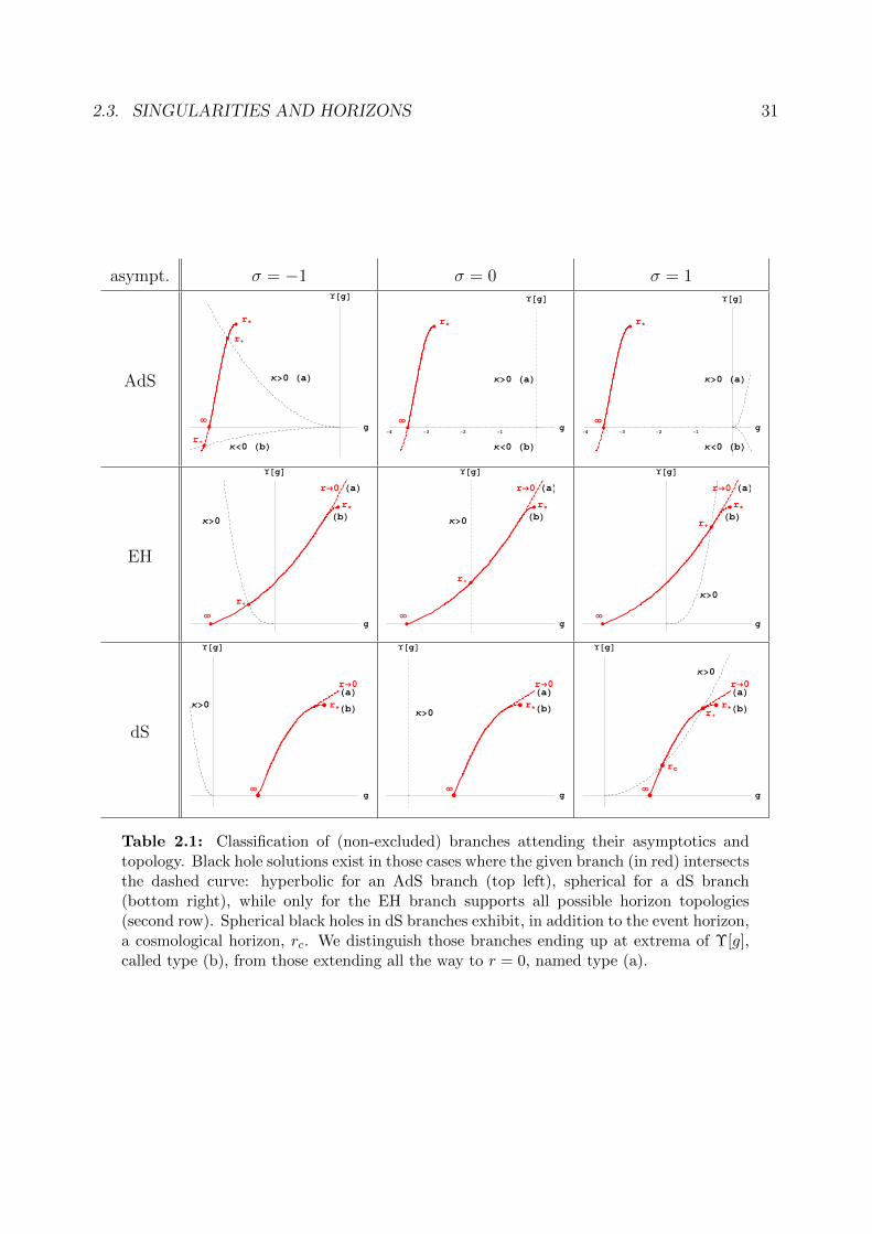
2.3. SINGULARITIES AND HORIZONS 31
asympt. σ = −1 σ = 0 σ = 1
AdS
g
U@gD
¥
r+
r+
r*
Κ<0 HbL
Κ>0 HaL
-4 -3 -2 -1g
U@gD
¥
r*
Κ<0 HbL
Κ>0 HaL
-4 -3 -2 -1g
U@gD
¥
r*
Κ<0 HbL
Κ>0 HaL
EH
g
U@gDr®0
r*
¥
r+
Κ>0
HaL
HbL
g
U@gDr®0
r*
¥
r+
Κ>0
HaL
HbL
g
U@gD
r+
r*
¥
r®0
Κ>0
HaL
HbL
dS
g
U@gD
¥
r*
r®0
Κ>0HaLHbL
g
U@gD
¥
r*
r®0
Κ>0
HaLHbL
g
U@gD
¥
r*
rc
r+
r®0Κ>0
HaLHbL
Table 2.1: Classification of (non-excluded) branches attending their asymptotics andtopology. Black hole solutions exist in those cases where the given branch (in red) intersectsthe dashed curve: hyperbolic for an AdS branch (top left), spherical for a dS branch(bottom right), while only for the EH branch supports all possible horizon topologies(second row). Spherical black holes in dS branches exhibit, in addition to the event horizon,a cosmological horizon, rc. We distinguish those branches ending up at extrema of Υ[g],called type (b), from those extending all the way to r = 0, named type (a).
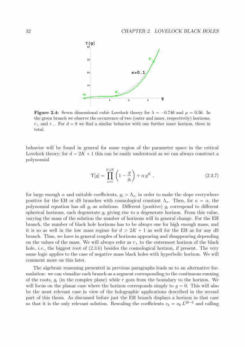
32 CHAPTER 2. LOVELOCK BLACK HOLES
2 4 6g
10
20
30
40
U@gD
¥r+
r-
Κ=0.1
Figure 2.4: Seven dimensional cubic Lovelock theory for λ = −0.746 and µ = 0.56. Inthe green branch we observe the occurrence of two (outer and inner, respectively) horizons,r+ and r−. For d = 8 we find a similar behavior with one further inner horizon, three intotal.
behavior will be found in general for some region of the parameter space in the criticalLovelock theory; for d = 2K + 1 this can be easily understood as we can always construct apolynomial
Υ[g] =
L≤K∏i=1
(1− g
gi
)+ α gK , (2.3.7)
for large enough α and suitable coefficients, gi > Λ?, in order to make the slope everywherepositive for the EH or dS branches with cosmological constant Λ?. Then, for κ = α, thepolynomial equation has all gi as solutions. Different (positive) gi correspond to differentspherical horizons, each degenerate gi giving rise to a degenerate horizon. From this value,varying the mass of the solution the number of horizons will in general change. For the EHbranch, the number of black hole horizons has to be always one for high enough mass, andit is so as well in the low mass regime for d > 2K + 1 as well for the EH as for any dSbranch. Thus, we have in general couples of horizons appearing and disappearing dependingon the values of the mass. We will always refer as r+ to the outermost horizon of the blackhole, i.e., the biggest root of (2.3.6) besides the cosmological horizon, if present. The verysame logic applies to the case of negative mass black holes with hyperbolic horizon. We willcomment more on this later.
The algebraic reasoning presented in previous paragraphs leads us to an alternative for-mulation: we can visualize each branch as a segment corresponding to the continuous runningof the roots, gi (in the complex plane) while r goes from the boundary to the horizon. Wewill focus on the planar case where the horizon corresponds simply to g = 0. This will alsobe the most relevant case in view of the holographic applications described in the secondpart of this thesis. As discussed before just the EH branch displays a horizon in that caseso that it is the only relevant solution. Rescaling the coefficients ck = ak L
2k−2 and calling
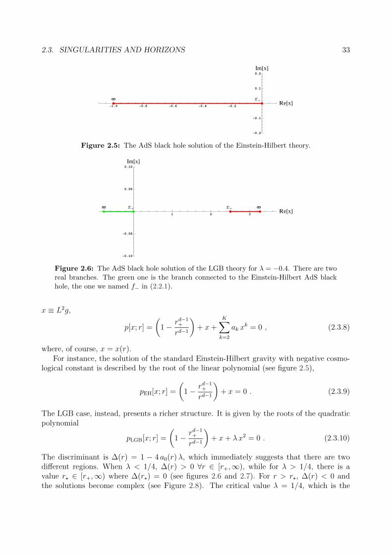
2.3. SINGULARITIES AND HORIZONS 33
-1.0 -0.8 -0.6 -0.4 -0.2Re@xD
-0.2
-0.1
0.1
0.2
Ám@xD
¥ r+
Figure 2.5: The AdS black hole solution of the Einstein-Hilbert theory.
1 2 3Re@xD
-0.10
-0.05
0.05
0.10
Ám@xD
¥r+¥ r+
Figure 2.6: The AdS black hole solution of the LGB theory for λ = −0.4. There are tworeal branches. The green one is the branch connected to the Einstein-Hilbert AdS blackhole, the one we named f− in (2.2.1).
x ≡ L2g,
p[x; r] =
(1− rd−1
+
rd−1
)+ x+
K∑k=2
ak xk = 0 , (2.3.8)
where, of course, x = x(r).For instance, the solution of the standard Einstein-Hilbert gravity with negative cosmo-
logical constant is described by the root of the linear polynomial (see figure 2.5),
pEH[x; r] =
(1− rd−1
+
rd−1
)+ x = 0 . (2.3.9)
The LGB case, instead, presents a richer structure. It is given by the roots of the quadraticpolynomial
pLGB[x; r] =
(1− rd−1
+
rd−1
)+ x+ λx2 = 0 . (2.3.10)
The discriminant is ∆(r) = 1 − 4 a0(r)λ, which immediately suggests that there are twodifferent regions. When λ < 1/4, ∆(r) > 0 ∀r ∈ [r+,∞), while for λ > 1/4, there is avalue r? ∈ [r+,∞) where ∆(r?) = 0 (see figures 2.6 and 2.7). For r > r?, ∆(r) < 0 andthe solutions become complex (see Figure 2.8). The critical value λ = 1/4, which is the
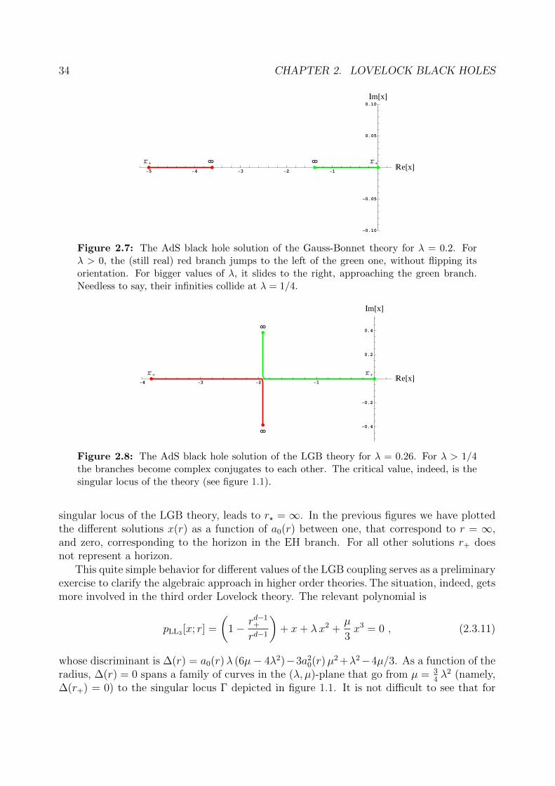
34 CHAPTER 2. LOVELOCK BLACK HOLES
-5 -4 -3 -2 -1Re@xD
-0.10
-0.05
0.05
0.10
Ám@xD
¥r+ ¥ r+
Figure 2.7: The AdS black hole solution of the Gauss-Bonnet theory for λ = 0.2. Forλ > 0, the (still real) red branch jumps to the left of the green one, without flipping itsorientation. For bigger values of λ, it slides to the right, approaching the green branch.Needless to say, their infinities collide at λ = 1/4.
-4 -3 -2 -1Re@xD
-0.4
-0.2
0.2
0.4
Ám@xD
¥
r+
¥
r+
Figure 2.8: The AdS black hole solution of the LGB theory for λ = 0.26. For λ > 1/4the branches become complex conjugates to each other. The critical value, indeed, is thesingular locus of the theory (see figure 1.1).
singular locus of the LGB theory, leads to r? = ∞. In the previous figures we have plottedthe different solutions x(r) as a function of a0(r) between one, that correspond to r = ∞,and zero, corresponding to the horizon in the EH branch. For all other solutions r+ doesnot represent a horizon.
This quite simple behavior for different values of the LGB coupling serves as a preliminaryexercise to clarify the algebraic approach in higher order theories. The situation, indeed, getsmore involved in the third order Lovelock theory. The relevant polynomial is
pLL3 [x; r] =
(1− rd−1
+
rd−1
)+ x+ λx2 +
µ
3x3 = 0 , (2.3.11)
whose discriminant is ∆(r) = a0(r)λ (6µ− 4λ2)−3a20(r)µ2 +λ2−4µ/3. As a function of the
radius, ∆(r) = 0 spans a family of curves in the (λ, µ)-plane that go from µ = 34λ2 (namely,
∆(r+) = 0) to the singular locus Γ depicted in figure 1.1. It is not difficult to see that for
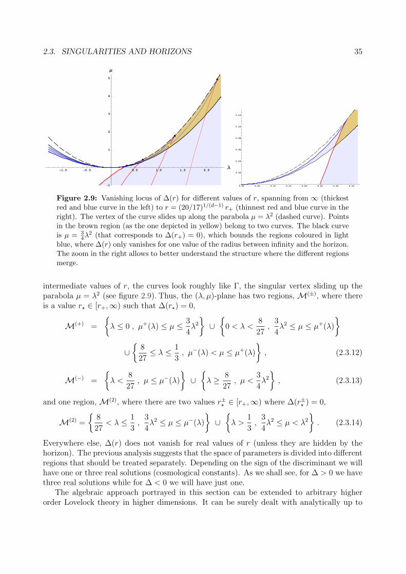
2.3. SINGULARITIES AND HORIZONS 35
-1.0 -0.5 0.5 1.0 1.5 2.0Λ
-1
1
2
3
4
5
Μ
0.00 0.05 0.10 0.15 0.20 0.25 0.30 0.35
0.02
0.04
0.06
0.08
0.10
0.12
Figure 2.9: Vanishing locus of ∆(r) for different values of r, spanning from ∞ (thickestred and blue curve in the left) to r = (20/17)1/(d−1) r+ (thinnest red and blue curve in theright). The vertex of the curve slides up along the parabola µ = λ2 (dashed curve). Pointsin the brown region (as the one depicted in yellow) belong to two curves. The black curveis µ = 3
4λ2 (that corresponds to ∆(r+) = 0), which bounds the regions coloured in light
blue, where ∆(r) only vanishes for one value of the radius between infinity and the horizon.The zoom in the right allows to better understand the structure where the different regionsmerge.
intermediate values of r, the curves look roughly like Γ, the singular vertex sliding up theparabola µ = λ2 (see figure 2.9). Thus, the (λ, µ)-plane has two regions, M(±), where thereis a value r? ∈ [r+,∞) such that ∆(r?) = 0,
M(+) =
λ ≤ 0 , µ+(λ) ≤ µ ≤ 3
4λ2
∪
0 < λ <8
27,
3
4λ2 ≤ µ ≤ µ+(λ)
∪
8
27≤ λ ≤ 1
3, µ−(λ) < µ ≤ µ+(λ)
, (2.3.12)
M(−) =
λ <
8
27, µ ≤ µ−(λ)
∪λ ≥ 8
27, µ <
3
4λ2
, (2.3.13)
and one region, M(2), where there are two values r±? ∈ [r+,∞) where ∆(r±? ) = 0,
M(2) =
8
27< λ ≤ 1
3,
3
4λ2 ≤ µ ≤ µ−(λ)
∪λ >
1
3,
3
4λ2 ≤ µ < λ2
. (2.3.14)
Everywhere else, ∆(r) does not vanish for real values of r (unless they are hidden by thehorizon). The previous analysis suggests that the space of parameters is divided into differentregions that should be treated separately. Depending on the sign of the discriminant we willhave one or three real solutions (cosmological constants). As we shall see, for ∆ > 0 we havethree real solutions while for ∆ < 0 we will have just one.
The algebraic approach portrayed in this section can be extended to arbitrary higherorder Lovelock theory in higher dimensions. It can be surely dealt with analytically up to
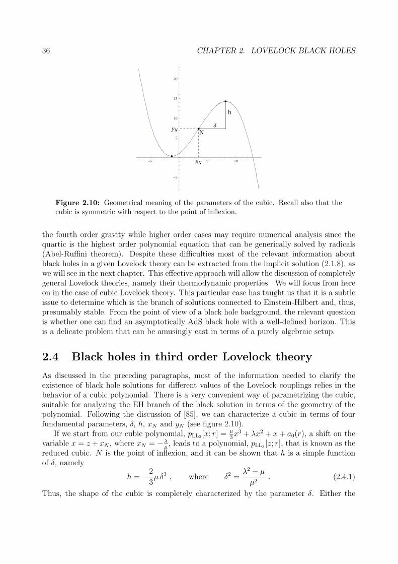
36 CHAPTER 2. LOVELOCK BLACK HOLES
-5 5 10
-5
5
10
15
20
N
xN
yN∆
h
Figure 2.10: Geometrical meaning of the parameters of the cubic. Recall also that thecubic is symmetric with respect to the point of inflexion.
the fourth order gravity while higher order cases may require numerical analysis since thequartic is the highest order polynomial equation that can be generically solved by radicals(Abel-Ruffini theorem). Despite these difficulties most of the relevant information aboutblack holes in a given Lovelock theory can be extracted from the implicit solution (2.1.8), aswe will see in the next chapter. This effective approach will allow the discussion of completelygeneral Lovelock theories, namely their thermodynamic properties. We will focus from hereon in the case of cubic Lovelock theory. This particular case has taught us that it is a subtleissue to determine which is the branch of solutions connected to Einstein-Hilbert and, thus,presumably stable. From the point of view of a black hole background, the relevant questionis whether one can find an asymptotically AdS black hole with a well-defined horizon. Thisis a delicate problem that can be amusingly cast in terms of a purely algebraic setup.
2.4 Black holes in third order Lovelock theory
As discussed in the preceding paragraphs, most of the information needed to clarify theexistence of black hole solutions for different values of the Lovelock couplings relies in thebehavior of a cubic polynomial. There is a very convenient way of parametrizing the cubic,suitable for analyzing the EH branch of the black solution in terms of the geometry of thepolynomial. Following the discussion of [85], we can characterize a cubic in terms of fourfundamental parameters, δ, h, xN and yN (see figure 2.10).
If we start from our cubic polynomial, pLL3 [x; r] = µ3x3 + λx2 + x+ a0(r), a shift on the
variable x = z + xN , where xN = −λµ, leads to a polynomial, pLL3 [z; r], that is known as the
reduced cubic. N is the point of inflexion, and it can be shown that h is a simple functionof δ, namely
h = −2
3µ δ3 , where δ2 =
λ2 − µµ2
. (2.4.1)
Thus, the shape of the cubic is completely characterized by the parameter δ. Either the
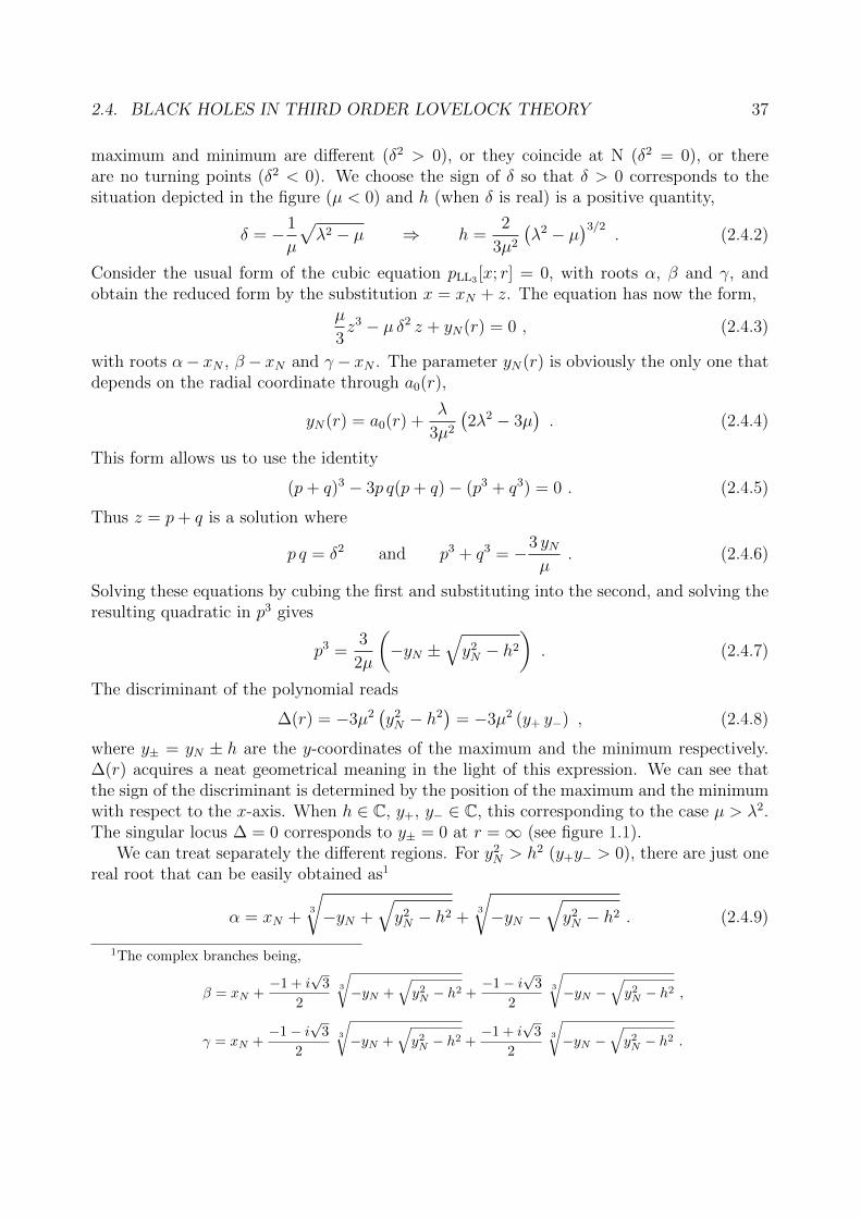
2.4. BLACK HOLES IN THIRD ORDER LOVELOCK THEORY 37
maximum and minimum are different (δ2 > 0), or they coincide at N (δ2 = 0), or thereare no turning points (δ2 < 0). We choose the sign of δ so that δ > 0 corresponds to thesituation depicted in the figure (µ < 0) and h (when δ is real) is a positive quantity,
δ = − 1
µ
√λ2 − µ ⇒ h =
2
3µ2
(λ2 − µ
)3/2. (2.4.2)
Consider the usual form of the cubic equation pLL3 [x; r] = 0, with roots α, β and γ, andobtain the reduced form by the substitution x = xN + z. The equation has now the form,
µ
3z3 − µ δ2 z + yN(r) = 0 , (2.4.3)
with roots α− xN , β − xN and γ − xN . The parameter yN(r) is obviously the only one thatdepends on the radial coordinate through a0(r),
yN(r) = a0(r) +λ
3µ2
(2λ2 − 3µ
). (2.4.4)
This form allows us to use the identity
(p+ q)3 − 3p q(p+ q)− (p3 + q3) = 0 . (2.4.5)
Thus z = p+ q is a solution where
p q = δ2 and p3 + q3 = −3 yNµ
. (2.4.6)
Solving these equations by cubing the first and substituting into the second, and solving theresulting quadratic in p3 gives
p3 =3
2µ
(−yN ±
√y2N − h2
). (2.4.7)
The discriminant of the polynomial reads
∆(r) = −3µ2(y2N − h2
)= −3µ2 (y+ y−) , (2.4.8)
where y± = yN ± h are the y-coordinates of the maximum and the minimum respectively.∆(r) acquires a neat geometrical meaning in the light of this expression. We can see thatthe sign of the discriminant is determined by the position of the maximum and the minimumwith respect to the x-axis. When h ∈ C, y+, y− ∈ C, this corresponding to the case µ > λ2.The singular locus ∆ = 0 corresponds to y± = 0 at r =∞ (see figure 1.1).
We can treat separately the different regions. For y2N > h2 (y+y− > 0), there are just one
real root that can be easily obtained as1
α = xN +3
√−yN +
√y2N − h2 +
3
√−yN −
√y2N − h2 . (2.4.9)
1The complex branches being,
β = xN +−1 + i
√3
2
3
√−yN +
√y2N − h2 +
−1− i√
3
2
3
√−yN −
√y2N − h2 ,
γ = xN +−1− i
√3
2
3
√−yN +
√y2N − h2 +
−1 + i√
3
2
3
√−yN −
√y2N − h2 .
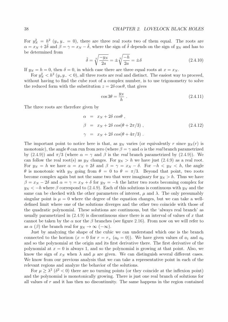
38 CHAPTER 2. LOVELOCK BLACK HOLES
For y2N = h2 (y+ y− = 0), there are three real roots two of them equal. The roots are
α = xN + 2δ and β = γ = xN − δ, where the sign of δ depends on the sign of yN and has tobe determined from
δ = 3
√−yN2a
= ± 3
√−h2a
= ±δ (2.4.10)
If yN = h = 0, then δ = 0, in which case there are three equal roots at x = xN .For y2
N < h2 (y+y− < 0), all three roots are real and distinct. The easiest way to proceed,without having to find the cube root of a complex number, is to use trigonometry to solvethe reduced form with the substitution z = 2δ cos θ, that gives
cos 3θ =yNh
. (2.4.11)
The three roots are therefore given by
α = xN + 2δ cosθ ,
β = xN + 2δ cos(θ + 2π/3) , (2.4.12)
γ = xN + 2δ cos(θ + 4π/3) .
The important point to notice here is that, as yN varies (or equivalently r since yN(r) ismonotonic), the angle θ can run from zero (where β = γ and α is the real branch parametrizedby (2.4.9)) and π/3 (where α = γ and β is the real branch parametrized by (2.4.9)). Wecan follow the real root(s) as yN changes. For yN > h we have just (2.4.9) as a real root.For yN = h we have α = xN + 2δ and β = γ = xN − δ. For −h < yN < h, the angleθ is monotonic with yN going from θ = 0 to θ = π/3. Beyond that point, two rootsbecome complex again but not the same two that were imaginary for yN > h. Thus we haveβ = xN − 2δ and α = γ = xN + δ for yN = −h the latter two roots becoming complex foryN < −h where β correspond to (2.4.9). Each of this solutions is continuous with yN and thesame can be checked with the other parameters of interest, µ and λ. The only presumablysingular point is µ = 0 where the degree of the equation changes, but we can take a well-defined limit where one of the solutions diverges and the other two coincide with those ofthe quadratic polynomial. These solutions are continuous, but the ‘always real branch’ asusually parametrized in (2.4.9) is discontinuous since there is an interval of values of x thatcannot be taken by the α nor the β branches (see figure 2.16). From now on we will refer toas α (β) the branch real for yN →∞ (−∞).
Just by analyzing the shape of the cubic we can understand which one is the branchconnected to the horizon (x = 0 for r = r+ (a0 = 0)). We have given values of a1 and a0
and so the polynomial at the origin and its first derivative there. The first derivative of thepolynomial at x = 0 is always 1, and so the polynomial is growing at that point. Also, weknow the sign of xN when λ and µ are given. We can distinguish several different cases.We know from our previous analysis that we can take a representative point in each of therelevant regions and analyze the behavior of the solutions.
For µ ≥ λ2 (δ2 < 0) there are no turning points (or they coincide at the inflexion point)and the polynomial is monotonically growing. There is just one real branch of solutions forall values of r and it has then no discontinuity. The same happens in the region contained
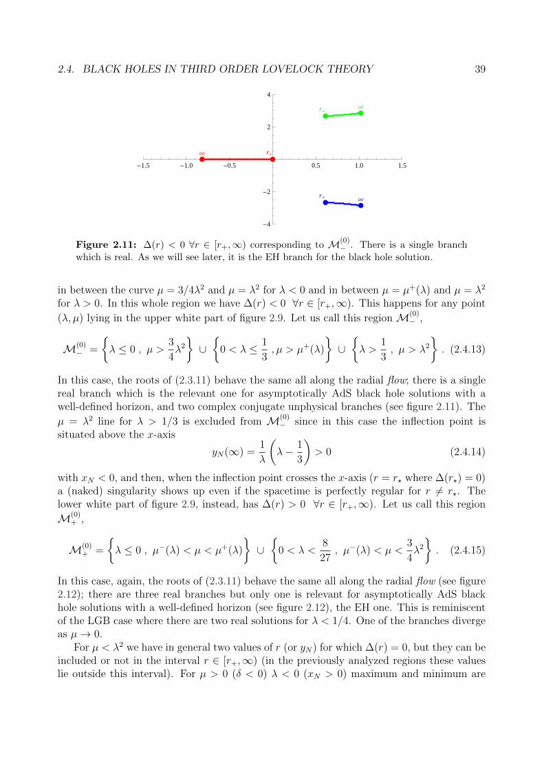
2.4. BLACK HOLES IN THIRD ORDER LOVELOCK THEORY 39
-1.5 -1.0 -0.5 0.5 1.0 1.5
-4
-2
2
4
¥ r+
¥r+
¥r+
Figure 2.11: ∆(r) < 0 ∀r ∈ [r+,∞) corresponding to M(0)− . There is a single branch
which is real. As we will see later, it is the EH branch for the black hole solution.
in between the curve µ = 3/4λ2 and µ = λ2 for λ < 0 and in between µ = µ+(λ) and µ = λ2
for λ > 0. In this whole region we have ∆(r) < 0 ∀r ∈ [r+,∞). This happens for any point
(λ, µ) lying in the upper white part of figure 2.9. Let us call this region M(0)− ,
M(0)− =
λ ≤ 0 , µ >
3
4λ2
∪
0 < λ ≤ 1
3, µ > µ+(λ)
∪λ >
1
3, µ > λ2
. (2.4.13)
In this case, the roots of (2.3.11) behave the same all along the radial flow; there is a singlereal branch which is the relevant one for asymptotically AdS black hole solutions with awell-defined horizon, and two complex conjugate unphysical branches (see figure 2.11). The
µ = λ2 line for λ > 1/3 is excluded from M(0)− since in this case the inflection point is
situated above the x-axis
yN(∞) =1
λ
(λ− 1
3
)> 0 (2.4.14)
with xN < 0, and then, when the inflection point crosses the x-axis (r = r? where ∆(r?) = 0)a (naked) singularity shows up even if the spacetime is perfectly regular for r 6= r?. Thelower white part of figure 2.9, instead, has ∆(r) > 0 ∀r ∈ [r+,∞). Let us call this region
M(0)+ ,
M(0)+ =
λ ≤ 0 , µ−(λ) < µ < µ+(λ)
∪
0 < λ <8
27, µ−(λ) < µ <
3
4λ2
. (2.4.15)
In this case, again, the roots of (2.3.11) behave the same all along the radial flow (see figure2.12); there are three real branches but only one is relevant for asymptotically AdS blackhole solutions with a well-defined horizon (see figure 2.12), the EH one. This is reminiscentof the LGB case where there are two real solutions for λ < 1/4. One of the branches divergeas µ→ 0.
For µ < λ2 we have in general two values of r (or yN) for which ∆(r) = 0, but they can beincluded or not in the interval r ∈ [r+,∞) (in the previously analyzed regions these valueslie outside this interval). For µ > 0 (δ < 0) λ < 0 (xN > 0) maximum and minimum are
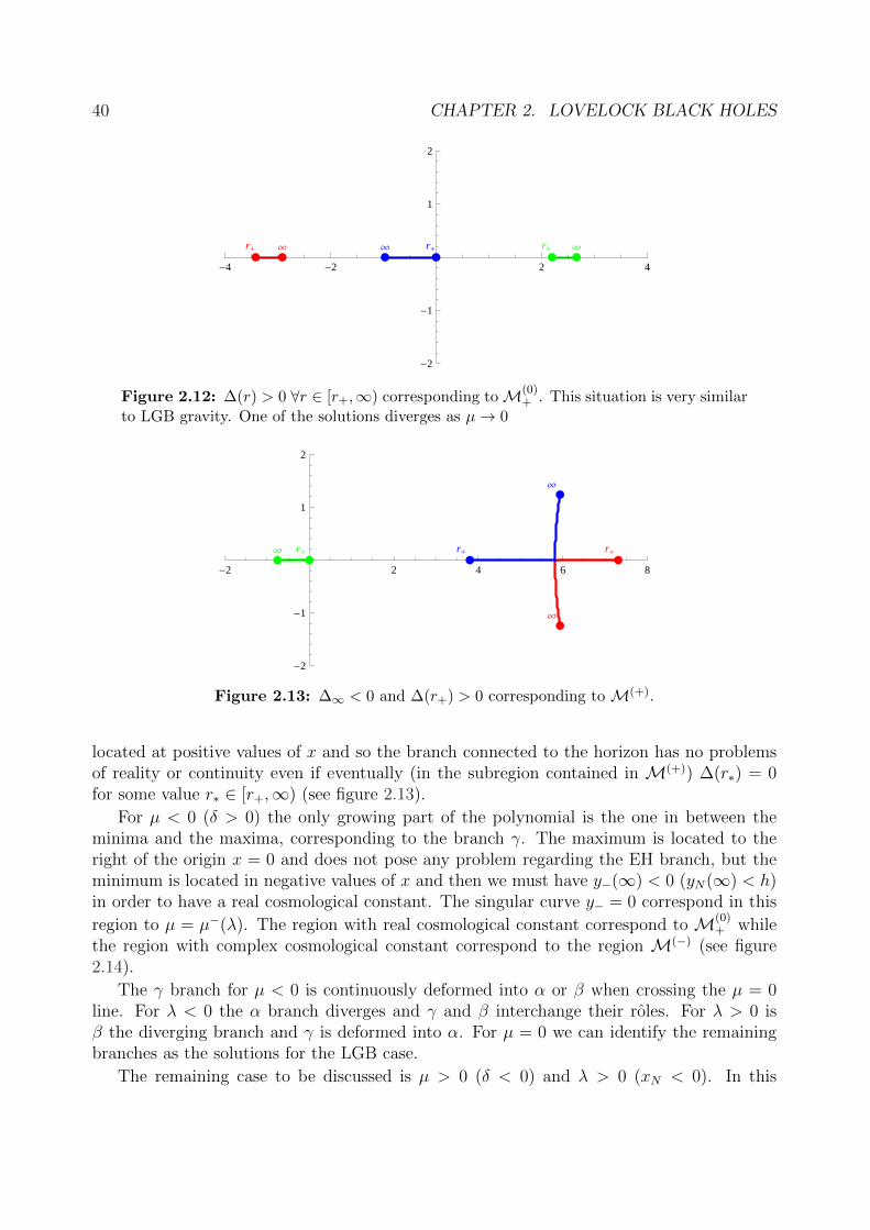
40 CHAPTER 2. LOVELOCK BLACK HOLES
-4 -2 2 4
-2
-1
1
2
¥r+ ¥r+¥ r+
Figure 2.12: ∆(r) > 0 ∀r ∈ [r+,∞) corresponding toM(0)+ . This situation is very similar
to LGB gravity. One of the solutions diverges as µ→ 0
-2 2 4 6 8
-2
-1
1
2
¥
r+¥ r+
¥
r+
Figure 2.13: ∆∞ < 0 and ∆(r+) > 0 corresponding to M(+).
located at positive values of x and so the branch connected to the horizon has no problemsof reality or continuity even if eventually (in the subregion contained in M(+)) ∆(r∗) = 0for some value r∗ ∈ [r+,∞) (see figure 2.13).
For µ < 0 (δ > 0) the only growing part of the polynomial is the one in between theminima and the maxima, corresponding to the branch γ. The maximum is located to theright of the origin x = 0 and does not pose any problem regarding the EH branch, but theminimum is located in negative values of x and then we must have y−(∞) < 0 (yN(∞) < h)in order to have a real cosmological constant. The singular curve y− = 0 correspond in this
region to µ = µ−(λ). The region with real cosmological constant correspond to M(0)+ while
the region with complex cosmological constant correspond to the region M(−) (see figure2.14).
The γ branch for µ < 0 is continuously deformed into α or β when crossing the µ = 0line. For λ < 0 the α branch diverges and γ and β interchange their roles. For λ > 0 isβ the diverging branch and γ is deformed into α. For µ = 0 we can identify the remainingbranches as the solutions for the LGB case.
The remaining case to be discussed is µ > 0 (δ < 0) and λ > 0 (xN < 0). In this
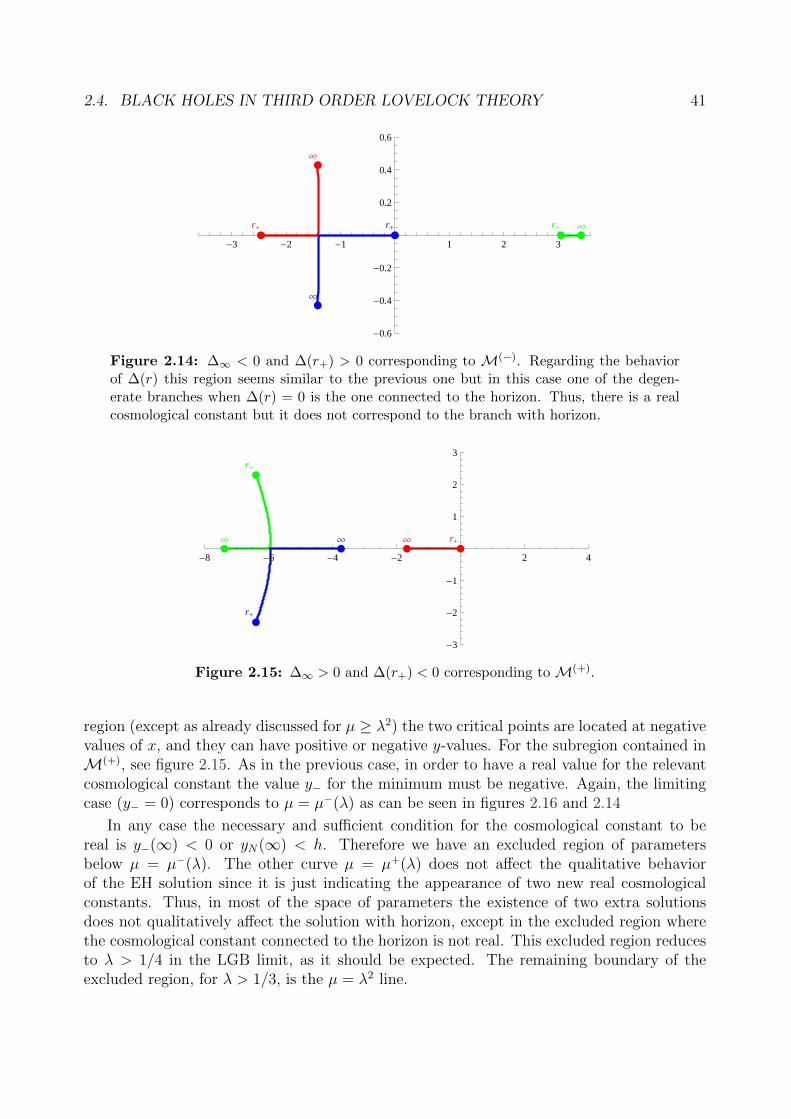
2.4. BLACK HOLES IN THIRD ORDER LOVELOCK THEORY 41
-3 -2 -1 1 2 3
-0.6
-0.4
-0.2
0.2
0.4
0.6
¥
r+ ¥r+
¥
r+
Figure 2.14: ∆∞ < 0 and ∆(r+) > 0 corresponding to M(−). Regarding the behaviorof ∆(r) this region seems similar to the previous one but in this case one of the degen-erate branches when ∆(r) = 0 is the one connected to the horizon. Thus, there is a realcosmological constant but it does not correspond to the branch with horizon.
-8 -6 -4 -2 2 4
-3
-2
-1
1
2
3
¥ r+¥
r+
¥
r+
Figure 2.15: ∆∞ > 0 and ∆(r+) < 0 corresponding to M(+).
region (except as already discussed for µ ≥ λ2) the two critical points are located at negativevalues of x, and they can have positive or negative y-values. For the subregion contained inM(+), see figure 2.15. As in the previous case, in order to have a real value for the relevantcosmological constant the value y− for the minimum must be negative. Again, the limitingcase (y− = 0) corresponds to µ = µ−(λ) as can be seen in figures 2.16 and 2.14
In any case the necessary and sufficient condition for the cosmological constant to bereal is y−(∞) < 0 or yN(∞) < h. Therefore we have an excluded region of parametersbelow µ = µ−(λ). The other curve µ = µ+(λ) does not affect the qualitative behaviorof the EH solution since it is just indicating the appearance of two new real cosmologicalconstants. Thus, in most of the space of parameters the existence of two extra solutionsdoes not qualitatively affect the solution with horizon, except in the excluded region wherethe cosmological constant connected to the horizon is not real. This excluded region reducesto λ > 1/4 in the LGB limit, as it should be expected. The remaining boundary of theexcluded region, for λ > 1/3, is the µ = λ2 line.
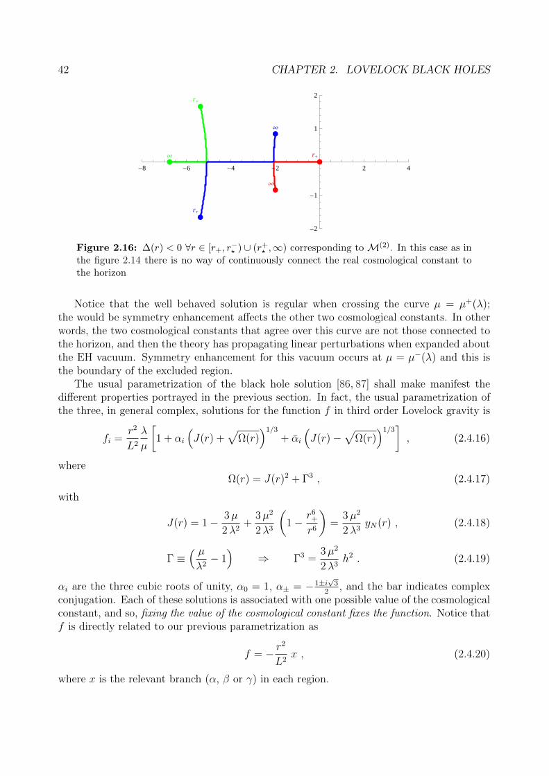
42 CHAPTER 2. LOVELOCK BLACK HOLES
-8 -6 -4 -2 2 4
-2
-1
1
2
¥
r+¥
r+
¥
r+
Figure 2.16: ∆(r) < 0 ∀r ∈ [r+, r−? ) ∪ (r+
? ,∞) corresponding to M(2). In this case as inthe figure 2.14 there is no way of continuously connect the real cosmological constant tothe horizon
Notice that the well behaved solution is regular when crossing the curve µ = µ+(λ);the would be symmetry enhancement affects the other two cosmological constants. In otherwords, the two cosmological constants that agree over this curve are not those connected tothe horizon, and then the theory has propagating linear perturbations when expanded aboutthe EH vacuum. Symmetry enhancement for this vacuum occurs at µ = µ−(λ) and this isthe boundary of the excluded region.
The usual parametrization of the black hole solution [86, 87] shall make manifest thedifferent properties portrayed in the previous section. In fact, the usual parametrization ofthe three, in general complex, solutions for the function f in third order Lovelock gravity is
fi =r2
L2
λ
µ
[1 + αi
(J(r) +
√Ω(r)
)1/3
+ αi
(J(r)−
√Ω(r)
)1/3], (2.4.16)
whereΩ(r) = J(r)2 + Γ3 , (2.4.17)
with
J(r) = 1− 3µ
2λ2+
3µ2
2λ3
(1−
r6+
r6
)=
3µ2
2λ3yN(r) , (2.4.18)
Γ ≡( µλ2− 1)
⇒ Γ3 =3µ2
2λ3h2 . (2.4.19)
αi are the three cubic roots of unity, α0 = 1, α± = −1±i√
32
, and the bar indicates complexconjugation. Each of these solutions is associated with one possible value of the cosmologicalconstant, and so, fixing the value of the cosmological constant fixes the function. Notice thatf is directly related to our previous parametrization as
f = − r2
L2x , (2.4.20)
where x is the relevant branch (α, β or γ) in each region.
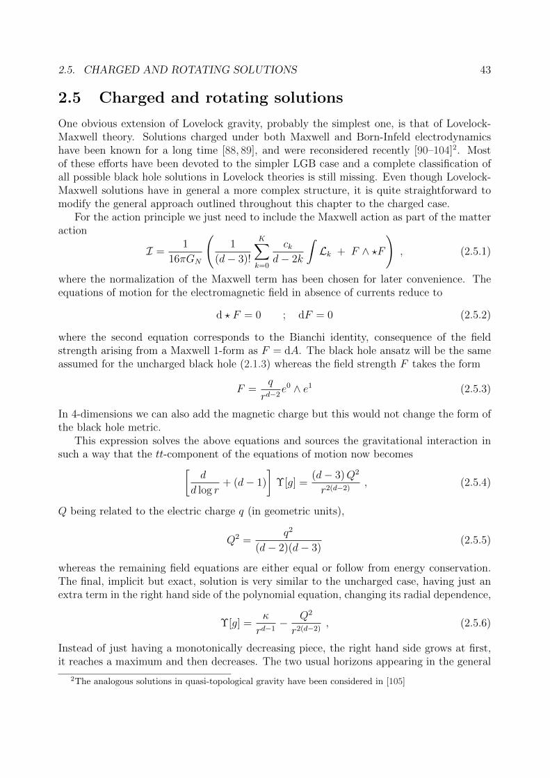
2.5. CHARGED AND ROTATING SOLUTIONS 43
2.5 Charged and rotating solutions
One obvious extension of Lovelock gravity, probably the simplest one, is that of Lovelock-Maxwell theory. Solutions charged under both Maxwell and Born-Infeld electrodynamicshave been known for a long time [88, 89], and were reconsidered recently [90–104]2. Mostof these efforts have been devoted to the simpler LGB case and a complete classification ofall possible black hole solutions in Lovelock theories is still missing. Even though Lovelock-Maxwell solutions have in general a more complex structure, it is quite straightforward tomodify the general approach outlined throughout this chapter to the charged case.
For the action principle we just need to include the Maxwell action as part of the matteraction
I =1
16πGN
(1
(d− 3)!
K∑k=0
ckd− 2k
∫Lk + F ∧ ?F
), (2.5.1)
where the normalization of the Maxwell term has been chosen for later convenience. Theequations of motion for the electromagnetic field in absence of currents reduce to
d ? F = 0 ; dF = 0 (2.5.2)
where the second equation corresponds to the Bianchi identity, consequence of the fieldstrength arising from a Maxwell 1-form as F = dA. The black hole ansatz will be the sameassumed for the uncharged black hole (2.1.3) whereas the field strength F takes the form
F =q
rd−2e0 ∧ e1 (2.5.3)
In 4-dimensions we can also add the magnetic charge but this would not change the form ofthe black hole metric.
This expression solves the above equations and sources the gravitational interaction insuch a way that the tt-component of the equations of motion now becomes[
d
d log r+ (d− 1)
]Υ[g] =
(d− 3)Q2
r2(d−2), (2.5.4)
Q being related to the electric charge q (in geometric units),
Q2 =q2
(d− 2)(d− 3)(2.5.5)
whereas the remaining field equations are either equal or follow from energy conservation.The final, implicit but exact, solution is very similar to the uncharged case, having just anextra term in the right hand side of the polynomial equation, changing its radial dependence,
Υ[g] =κ
rd−1− Q2
r2(d−2), (2.5.6)
Instead of just having a monotonically decreasing piece, the right hand side grows at first,it reaches a maximum and then decreases. The two usual horizons appearing in the general
2The analogous solutions in quasi-topological gravity have been considered in [105]
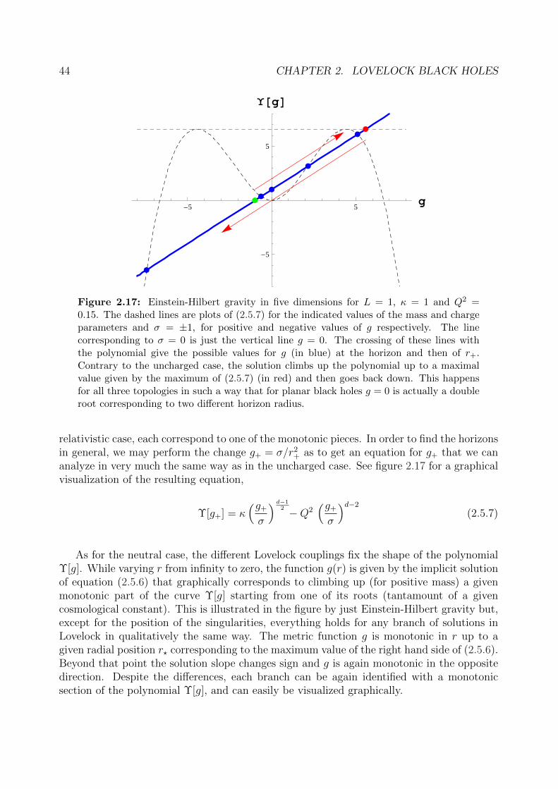
44 CHAPTER 2. LOVELOCK BLACK HOLES
-5 5g
-5
5
U@gD
Figure 2.17: Einstein-Hilbert gravity in five dimensions for L = 1, κ = 1 and Q2 =0.15. The dashed lines are plots of (2.5.7) for the indicated values of the mass and chargeparameters and σ = ±1, for positive and negative values of g respectively. The linecorresponding to σ = 0 is just the vertical line g = 0. The crossing of these lines withthe polynomial give the possible values for g (in blue) at the horizon and then of r+.Contrary to the uncharged case, the solution climbs up the polynomial up to a maximalvalue given by the maximum of (2.5.7) (in red) and then goes back down. This happensfor all three topologies in such a way that for planar black holes g = 0 is actually a doubleroot corresponding to two different horizon radius.
relativistic case, each correspond to one of the monotonic pieces. In order to find the horizonsin general, we may perform the change g+ = σ/r2
+ as to get an equation for g+ that we cananalyze in very much the same way as in the uncharged case. See figure 2.17 for a graphicalvisualization of the resulting equation,
Υ[g+] = κ(g+
σ
) d−12 −Q2
(g+
σ
)d−2
(2.5.7)
As for the neutral case, the different Lovelock couplings fix the shape of the polynomialΥ[g]. While varying r from infinity to zero, the function g(r) is given by the implicit solutionof equation (2.5.6) that graphically corresponds to climbing up (for positive mass) a givenmonotonic part of the curve Υ[g] starting from one of its roots (tantamount of a givencosmological constant). This is illustrated in the figure by just Einstein-Hilbert gravity but,except for the position of the singularities, everything holds for any branch of solutions inLovelock in qualitatively the same way. The metric function g is monotonic in r up to agiven radial position r? corresponding to the maximum value of the right hand side of (2.5.6).Beyond that point the solution slope changes sign and g is again monotonic in the oppositedirection. Despite the differences, each branch can be again identified with a monotonicsection of the polynomial Υ[g], and can easily be visualized graphically.
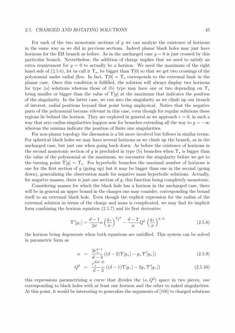
2.5. CHARGED AND ROTATING SOLUTIONS 45
For each of the two monotonic sections of g we can analyze the existence of horizonsin the same way as we did in previous sections. Indeed planar black holes may just havehorizons for the EH branch as before. As in the uncharged case g = 0 is just crossed by thisparticular branch. Nevertheless, the addition of charge implies that we need to satisfy anextra requirement for g = 0 to actually be a horizon. We need the maximum of the righthand side of (2.5.6), let us call it Υ?, be bigger than Υ[0] so that we get two crossings of thepolynomial under radial flow. In fact, Υ[0] = Υ? corresponds to the extremal limit in theplanar case. Once this condition is fulfilled, the solution will always display two horizonsfor type (a) solutions whereas those of (b) type may have one or two depending on Υ?
being smaller or bigger than the value of Υ[g] at the maximum that indicates the positionof the singularity. In the latter case, we run into the singularity as we climb up our branchof interest, radial positions beyond that point being unphysical. Notice that the negativeparts of the polynomial become relevant in this case, even though for regular solutions theseregions lie behind the horizon. They are explored in general as we approach r = 0, in such away that zero radius singularities happen now for branches extending all the way to g = −∞whereas the minima indicate the position of finite size singularities.
For non-planar topology the discussion is a bit more involved but follows in similar terms.For spherical black holes we may have several horizons as we climb up the branch, as in theuncharged case, but just one when going back down. As before the existence of horizons inthe second monotonic section of g is precluded in type (b) branches when Υ? is bigger thanthe value of the polynomial at the maximum, we encounter the singularity before we get tothe turning point Υ[g] = Υ?. For hyperbolic branches the maximal number of horizons isone for the first section of g (going up) but it may be bigger than one in the second (goingdown), generalizing the observation made for negative mass hyperbolic solutions. Actually,for negative masses, there is just one section of g, this function being completely monotonic.
Considering masses for which the black hole has a horizon in the uncharged case, therewill be in general an upper bound in the charges one may consider, corresponding the bounditself to an extremal black hole. Even though the explicit expression for the radius of theextremal solution in terms of the charge and mass is complicated, we may find its implicitform combining the horizon equation (2.5.7) and its first derivative
Υ′[g+] =d− 1
2σκ(g+
σ
) d−32 − d− 2
σQ2(g+
σ
)d−3
(2.5.8)
the horizon being degenerate when both equations are satidfied. This system can be solvedin parametric form as
κ =2rd−1
+
d− 3((d− 2)Υ[g+]− g+Υ′[g+]) (2.5.9)
Q2 =r
2(d−2)+
d− 3((d− 1)Υ[g+]− 2g+Υ′[g+]) (2.5.10)
this expressions parametrizing a curve that divides the (κ,Q2) space in two pieces, onecorresponding to black holes with at least one horizon and the other to naked singularities.At this point, it would be interesting to generalize the arguments of [106] to charged solutions
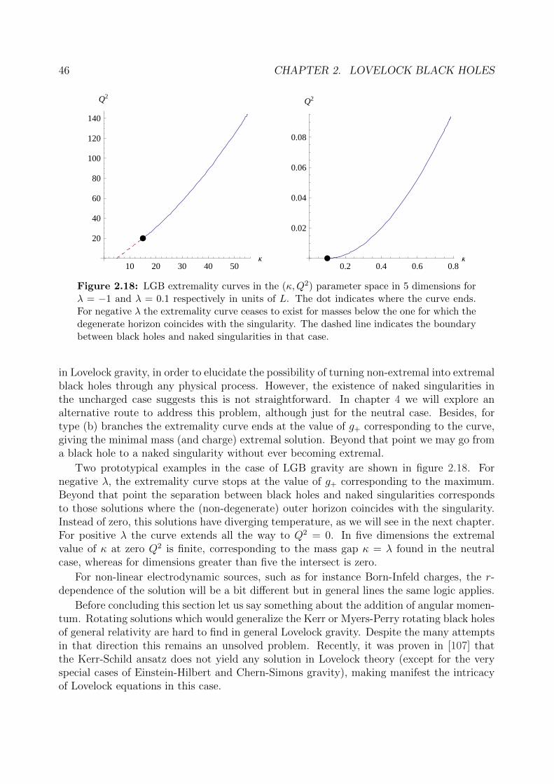
46 CHAPTER 2. LOVELOCK BLACK HOLES
10 20 30 40 50Κ
20
40
60
80
100
120
140
Q2
0.2 0.4 0.6 0.8Κ
0.02
0.04
0.06
0.08
Q2
Figure 2.18: LGB extremality curves in the (κ,Q2) parameter space in 5 dimensions forλ = −1 and λ = 0.1 respectively in units of L. The dot indicates where the curve ends.For negative λ the extremality curve ceases to exist for masses below the one for which thedegenerate horizon coincides with the singularity. The dashed line indicates the boundarybetween black holes and naked singularities in that case.
in Lovelock gravity, in order to elucidate the possibility of turning non-extremal into extremalblack holes through any physical process. However, the existence of naked singularities inthe uncharged case suggests this is not straightforward. In chapter 4 we will explore analternative route to address this problem, although just for the neutral case. Besides, fortype (b) branches the extremality curve ends at the value of g+ corresponding to the curve,giving the minimal mass (and charge) extremal solution. Beyond that point we may go froma black hole to a naked singularity without ever becoming extremal.
Two prototypical examples in the case of LGB gravity are shown in figure 2.18. Fornegative λ, the extremality curve stops at the value of g+ corresponding to the maximum.Beyond that point the separation between black holes and naked singularities correspondsto those solutions where the (non-degenerate) outer horizon coincides with the singularity.Instead of zero, this solutions have diverging temperature, as we will see in the next chapter.For positive λ the curve extends all the way to Q2 = 0. In five dimensions the extremalvalue of κ at zero Q2 is finite, corresponding to the mass gap κ = λ found in the neutralcase, whereas for dimensions greater than five the intersect is zero.
For non-linear electrodynamic sources, such as for instance Born-Infeld charges, the r-dependence of the solution will be a bit different but in general lines the same logic applies.
Before concluding this section let us say something about the addition of angular momen-tum. Rotating solutions which would generalize the Kerr or Myers-Perry rotating black holesof general relativity are hard to find in general Lovelock gravity. Despite the many attemptsin that direction this remains an unsolved problem. Recently, it was proven in [107] thatthe Kerr-Schild ansatz does not yield any solution in Lovelock theory (except for the veryspecial cases of Einstein-Hilbert and Chern-Simons gravity), making manifest the intricacyof Lovelock equations in this case.
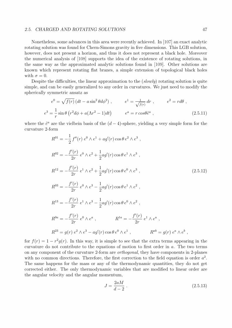
2.5. CHARGED AND ROTATING SOLUTIONS 47
Nonetheless, some advances in this area were recently achieved. In [107] an exact analyticrotating solution was found for Chern-Simons gravity in five dimensions. This LGB solution,however, does not present a horizon, and thus it does not represent a black hole. Moreoverthe numerical analysis of [108] supports the idea of the existence of rotating solutions, inthe same way as the approximated analytic solutions found in [109]. Other solutions areknown which represent rotating flat branes, a simple extension of topological black holeswith σ = 0.
Despite the difficulties, the linear approximation to the (slowly) rotating solution is quitesimple, and can be easily generalized to any order in curvatures. We just need to modify thespherically symmetric ansatz as
e0 =√f(r) (dt− a sin2 θdφ2) , e1 = 1√
f(r)dr , e2 = rdθ ,
e3 =1
rsin θ
(r2dφ+ a(Λr2 − 1)dt
)ea = r cosθea , (2.5.11)
where the ea are the vielbein basis of the (d− 4)-sphere, yielding a very simple form for thecurvature 2-form
R01 = −1
2f ′′(r) e0 ∧ e1 + ag′(r) cos θ e2 ∧ e3 ,
R02 = −f′(r)
2re0 ∧ e2 +
1
2ag′(r) cos θ e1 ∧ e3 ,
R12 = −f′(r)
2re1 ∧ e2 +
1
2ag′(r) cos θ e0 ∧ e3 , (2.5.12)
R03 = −f′(r)
2re0 ∧ e3 − 1
2ag′(r) cos θ e1 ∧ e2 ,
R13 = −f′(r)
2re1 ∧ e3 − 1
2ag′(r) cos θ e0 ∧ e2 ,
R0a = −f′(r)
2re0 ∧ ea , R1a = −f
′(r)
2re1 ∧ ea ,
R23 = g(r) e2 ∧ e3 − ag′(r) cos θ e0 ∧ e1 , Rab = g(r) ea ∧ eb ,
for f(r) = 1− r2g(r). In this way, it is simple to see that the extra terms appearing in thecurvature do not contribute to the equations of motion to first order in a. The two termson any component of the curvature 2-form are orthogonal, they have components in 2-planeswith no common directions. Therefore, the first correction to the field equation is order a2.The same happens for the mass or any of the thermodynamic quantities, they do not getcorrected either. The only thermodynamic variables that are modified to linear order arethe angular velocity and the angular momentum,
J =2aM
d− 2. (2.5.13)
48 CHAPTER 2. LOVELOCK BLACK HOLES
The obtained metric becomes
ds2 = −f(r)dt2 +dr2
f(r)+ r2dΩ2
d−1 − 2ar2 sin2 θ(g(r)− Λ)dtdφ (2.5.14)
with an undetermined constant Λ related to the angular velocity at infinity. We may chooseΛ to be the effective cosmological constant of the branch under study, g(∞) = Λ, in such away that this angular velocity vanishes,
Ω∞ =gtφgφφ
= ar2(g(r)− Λ) → 0 . (2.5.15)
At the horizon however the angular velocity is nonzero,
ΩH = a(1− r2+Λ) . (2.5.16)
2.6 Lovelock cosmologies
Another particularly simple solution in the context of Lovelock gravities are FRW cosmolo-gies. We may still use the same graphical techniques to describe and analyze them. Weconsider the usual homogeneous FRW ansatz
ds2 = −dt2 + a(t)2dΣ2d−1,σ , (2.6.1)
whose natural vielbein basis and resulting spin connection correspond to
e0 = dt , ea = a(t)ea , (2.6.2)
ωa0 =a
aea , ωab = ωab , (2.6.3)
where (ea, ωab) are the vielbein and spin connection of the maximally symmetric slices. Thischoice yields a particularly simple form for the curvature 2-form,
R0a =a
ae0 ∧ ea , Rab =
σ + a2
a2ea ∧ eb . (2.6.4)
The equations of motion are also very simple, diagonal, the tt-component being proportionalto the characteristic polynomial of the Lovelock theory, Υ[G], the argument function G beingin this case G = σ+a2
a2 (the role of the f function of the black hole being played by −a2).The rest of the components are fixed by the Bianchi identity to
Eb ∼[
d
d log a+ (d− 1)
]Υ[G] . (2.6.5)
The vacuum solutions are in this way exactly the same ones we found using the black holeansatz, i.e. maximally symmetric solutions with
σ + a2
a2=a
a= Λ . (2.6.6)
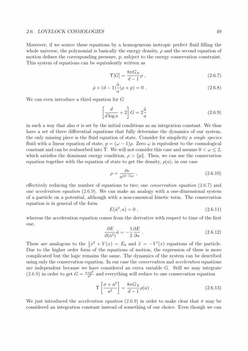
2.6. LOVELOCK COSMOLOGIES 49
Moreover, if we source these equations by a homogeneous isotropic perfect fluid filling thewhole universe, the polynomial is basically the energy density, ρ and the second equation ofmotion defines the corresponding pressure, p, subject to the energy conservation constraint.This system of equations can be equivalently written as
Υ[G] =8πGN
d− 1ρ , (2.6.7)
ρ+ (d− 1)a
a(ρ+ p) = 0 . (2.6.8)
We can even introduce a third equation for G[d
d log a+ 2
]G = 2
a
a(2.6.9)
in such a way that also σ is set by the initial conditions as an integration constant. We thushave a set of three differential equations that fully determine the dynamics of our system,the only missing piece is the fluid equation of state. Consider for simplicity a single speciesfluid with a linear equation of state, p = (ω − 1)ρ. Zero ω is equivalent to the cosmologicalconstant and can be reabsorbed into Υ. We will not consider this case and assume 0 < ω ≤ 2,which satisfies the dominant energy condition, ρ > ‖p‖. Then, we can use the conservationequation together with the equation of state to get the density, ρ(a), in our case
ρ =ρ0
a(d−1)ω, (2.6.10)
effectively reducing the number of equations to two; one conservation equation (2.6.7) andone acceleration equation (2.6.9). We can make an analogy with a one-dimensional systemof a particle on a potential, although with a non-canonical kinetic term. The conservationequation is in general of the form
E(a2, a) = 0 , (2.6.11)
whereas the acceleration equation comes from the derivative with respect to time of the firstone,
∂E
∂(a2)a = −1
2
∂E
∂a. (2.6.12)
These are analogous to the 12x2 + V (x) = E0 and x = −V ′(x) equations of the particle.
Due to the higher order form of the equations of motion, the expression of these is morecomplicated but the logic remains the same. The dynamics of the system can be describedusing only the conservation equation. In our case the conservation and acceleration equationsare independent because we have considered an extra variable G. Still we may integrate(2.6.9) in order to get G = σ+a2
a2 and everything will reduce to one conservation equation
Υ
[σ + a2
a2
]=
8πGN
d− 1ρ(a) . (2.6.13)
We just introduced the acceleration equation (2.6.9) in order to make clear that σ may beconsidered an integration constant instead of something of our choice. Even though we can
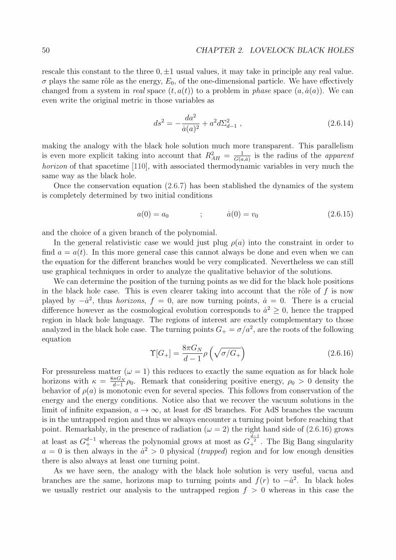
50 CHAPTER 2. LOVELOCK BLACK HOLES
rescale this constant to the three 0,±1 usual values, it may take in principle any real value.σ plays the same role as the energy, E0, of the one-dimensional particle. We have effectivelychanged from a system in real space (t, a(t)) to a problem in phase space (a, a(a)). We caneven write the original metric in those variables as
ds2 = − da2
a(a)2+ a2dΣ2
d−1 , (2.6.14)
making the analogy with the black hole solution much more transparent. This parallelismis even more explicit taking into account that R2
AH = 1G(a,a)
is the radius of the apparent
horizon of that spacetime [110], with associated thermodynamic variables in very much thesame way as the black hole.
Once the conservation equation (2.6.7) has been stablished the dynamics of the systemis completely determined by two initial conditions
a(0) = a0 ; a(0) = v0 (2.6.15)
and the choice of a given branch of the polynomial.
In the general relativistic case we would just plug ρ(a) into the constraint in order tofind a = a(t). In this more general case this cannot always be done and even when we canthe equation for the different branches would be very complicated. Nevertheless we can stilluse graphical techniques in order to analyze the qualitative behavior of the solutions.
We can determine the position of the turning points as we did for the black hole positionsin the black hole case. This is even clearer taking into account that the role of f is nowplayed by −a2, thus horizons, f = 0, are now turning points, a = 0. There is a crucialdifference however as the cosmological evolution corresponds to a2 ≥ 0, hence the trappedregion in black hole language. The regions of interest are exactly complementary to thoseanalyzed in the black hole case. The turning points G+ = σ/a2, are the roots of the followingequation
Υ[G+] =8πGN
d− 1ρ(√
σ/G+
)(2.6.16)
For pressureless matter (ω = 1) this reduces to exactly the same equation as for black holehorizons with κ = 8πGN
d−1ρ0. Remark that considering positive energy, ρ0 > 0 density the
behavior of ρ(a) is monotonic even for several species. This follows from conservation of theenergy and the energy conditions. Notice also that we recover the vacuum solutions in thelimit of infinite expansion, a→∞, at least for dS branches. For AdS branches the vacuumis in the untrapped region and thus we always encounter a turning point before reaching thatpoint. Remarkably, in the presence of radiation (ω = 2) the right hand side of (2.6.16) grows
at least as Gd−1+ whereas the polynomial grows at most as G
d−12
+ . The Big Bang singularitya = 0 is then always in the a2 > 0 physical (trapped) region and for low enough densitiesthere is also always at least one turning point.
As we have seen, the analogy with the black hole solution is very useful, vacua andbranches are the same, horizons map to turning points and f(r) to −a2. In black holeswe usually restrict our analysis to the untrapped region f > 0 whereas in this case the
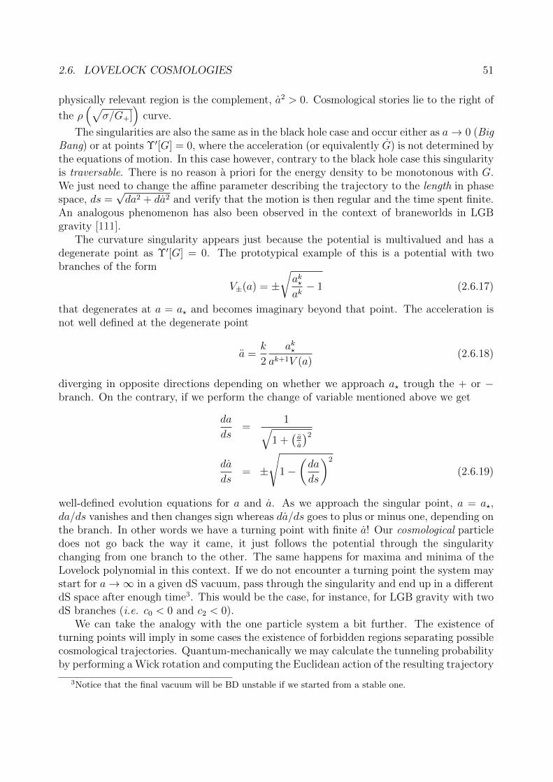
2.6. LOVELOCK COSMOLOGIES 51
physically relevant region is the complement, a2 > 0. Cosmological stories lie to the right of
the ρ(√
σ/G+])
curve.
The singularities are also the same as in the black hole case and occur either as a→ 0 (BigBang) or at points Υ′[G] = 0, where the acceleration (or equivalently G) is not determined bythe equations of motion. In this case however, contrary to the black hole case this singularityis traversable. There is no reason a priori for the energy density to be monotonous with G.We just need to change the affine parameter describing the trajectory to the length in phasespace, ds =
√da2 + da2 and verify that the motion is then regular and the time spent finite.
An analogous phenomenon has also been observed in the context of braneworlds in LGBgravity [111].
The curvature singularity appears just because the potential is multivalued and has adegenerate point as Υ′[G] = 0. The prototypical example of this is a potential with twobranches of the form
V±(a) = ±√ak?ak− 1 (2.6.17)
that degenerates at a = a? and becomes imaginary beyond that point. The acceleration isnot well defined at the degenerate point
a =k
2
ak?ak+1V (a)
(2.6.18)
diverging in opposite directions depending on whether we approach a? trough the + or −branch. On the contrary, if we perform the change of variable mentioned above we get
da
ds=
1√1 +
(aa
)2
da
ds= ±
√1−
(da
ds
)2
(2.6.19)
well-defined evolution equations for a and a. As we approach the singular point, a = a?,da/ds vanishes and then changes sign whereas da/ds goes to plus or minus one, depending onthe branch. In other words we have a turning point with finite a! Our cosmological particledoes not go back the way it came, it just follows the potential through the singularitychanging from one branch to the other. The same happens for maxima and minima of theLovelock polynomial in this context. If we do not encounter a turning point the system maystart for a→∞ in a given dS vacuum, pass through the singularity and end up in a differentdS space after enough time3. This would be the case, for instance, for LGB gravity with twodS branches (i.e. c0 < 0 and c2 < 0).
We can take the analogy with the one particle system a bit further. The existence ofturning points will imply in some cases the existence of forbidden regions separating possiblecosmological trajectories. Quantum-mechanically we may calculate the tunneling probabilityby performing a Wick rotation and computing the Euclidean action of the resulting trajectory
3Notice that the final vacuum will be BD unstable if we started from a stable one.
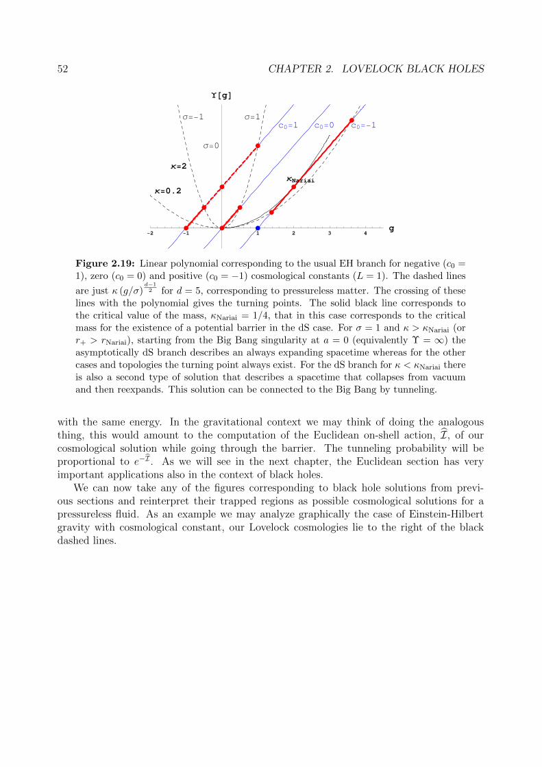
52 CHAPTER 2. LOVELOCK BLACK HOLES
-2 -1 1 2 3 4g
U@gD
Σ=1
Σ=0
Σ=-1c0=1 c0=0 c0=-1
Κ=2
Κ=0.2
ΚNariai
Figure 2.19: Linear polynomial corresponding to the usual EH branch for negative (c0 =1), zero (c0 = 0) and positive (c0 = −1) cosmological constants (L = 1). The dashed lines
are just κ (g/σ)d−1
2 for d = 5, corresponding to pressureless matter. The crossing of theselines with the polynomial gives the turning points. The solid black line corresponds tothe critical value of the mass, κNariai = 1/4, that in this case corresponds to the criticalmass for the existence of a potential barrier in the dS case. For σ = 1 and κ > κNariai (orr+ > rNariai), starting from the Big Bang singularity at a = 0 (equivalently Υ = ∞) theasymptotically dS branch describes an always expanding spacetime whereas for the othercases and topologies the turning point always exist. For the dS branch for κ < κNariai thereis also a second type of solution that describes a spacetime that collapses from vacuumand then reexpands. This solution can be connected to the Big Bang by tunneling.
with the same energy. In the gravitational context we may think of doing the analogousthing, this would amount to the computation of the Euclidean on-shell action, I, of ourcosmological solution while going through the barrier. The tunneling probability will beproportional to e−I . As we will see in the next chapter, the Euclidean section has veryimportant applications also in the context of black holes.
We can now take any of the figures corresponding to black hole solutions from previ-ous sections and reinterpret their trapped regions as possible cosmological solutions for apressureless fluid. As an example we may analyze graphically the case of Einstein-Hilbertgravity with cosmological constant, our Lovelock cosmologies lie to the right of the blackdashed lines.
Chapter 3
Black hole thermodynamics
“Pour atteindre la verite,il faut une fois dans la vie se defaire de toutes les opinions qu’on a recues,
et reconstruire de nouveau tout le systeme de ses connaissances.”
Rene Descartes
In the early 1970s, Bekenstein [112] argued, using simple thermodynamic arguments, thatblack holes should be assigned finite entropy, even though this seemed to contradict the factthat, as classical objects, they have zero temperature. Bekenstein was worried about thepossibility of collapsing matter into a black hole – classically, a very simple object – hidingany trace of the original entropy. The second law of thermodynamics, which asserts that theentropy of any closed system can never decrease, would be violated by this process. However,the mass increase due to the matter falling in also implies a growth of the black hole size,which led to the suggestion that the entropy of a black hole is given by its surface. Thisintuition became conviction when, in 1972, Hawking proved that the area of a black holeevent horizon can never decrease.
The similarity between black holes and thermodynamic systems was considerably strength-ened when Bardeen, Carter, and Hawking [113] showed that these enigmatic objects obey acomplete set of rules that parallel precisely the laws of thermodynamics,
• The surface gravity κ is constant over the event horizon (zeroth law).
• For any two stationary black holes differing only by small variations in the mass M ,angular momentum J , and charge Q,
δM =κ
8πGN
δA+ ΩHδJ + ΦHδQ (3.0.1)
53
54 CHAPTER 3. BLACK HOLE THERMODYNAMICS
where ΩH and ΦH are the angular velocity and the electromagnetic potential at thehorizon respectively (first law).
• The area of the event horizon of a black hole never decreases (second law),
δA ≥ 0 (3.0.2)
• It is impossible by any procedure to reduce the surface gravity κ to zero in a finitenumber of steps (third law).
These laws were later shown to apply in much more diverse situations than the particular4-dimensional setting where they were discovered. In particular, the first law holds for muchmore general gravitational actions, for which the entropy can be understood as a Noethercharge [114].
In these laws the role of the temperature is played by the surface gravity but Bardeen,Carter and Hawking, in their original paper, added: “It should however be emphasized thatκ/8πGN and A are distinct from the temperature and the entropy of the black hole. In factthe effective temperature of a black hole is absolute zero. In this sense a black hole can besaid to transcend the second law of thermodynamics.”
At the time, there seemed to be a fundamental contradiction between the hypothesis ofblack holes’ entropy being nonzero and them being perfectly absorptive entities. In contactwith a heat bath they would take in energy while giving off nothing, thus behaving as zerotemperature objects. Couple of years later, Hawking himself came up with the resolution ofthis apparent paradox, the problem being solved by quantum theory [115]. In the presence ofa horizon quantum fields were shown to be emitted with a thermal spectrum of temperaturegiven roughly by the surface gravity of the hole, TH = κ/2π. This temperature has notyet been directly observed, otherwise it would presumably grant Hawking the Nobel prize!For typical black hole masses, Hawking’s temperature is several orders of magnitude smallerthan the cosmic microwave background, thus impossible to measure. To have a Hawkingtemperature larger than 2.7 K (and actually be able to evaporate), a black hole needs tohave less mass than the Moon. Such a black hole would be smaller than a needle’s eye1.
All the accumulating evidence indicate that the similarities between the laws of blackhole mechanics and the laws of thermodynamics are not a simple coincidence. Indeed, theyseem to be hints of some very deep physics, intertwining classical and quantum propertiesof these objects. Hawking established the equivalence of surface gravity and temperatureof a black hole, whereas mass in this latter context is matched by the energy of the ther-modynamic system. Moreover, this connection also requires identifying the black hole areawith its entropy, as suggested by Bekenstein. More specifically, Bekenstein’s entropy is pro-portional to the area of the event horizon of the black hole. The Generalized Second Lawof thermodynamics then conjectures that the sum of the entropy of the matter outside ablack hole and its own never decreases. Moreover, black holes, as isolated objects, can bedescribed as thermodynamic ensembles to which all the usual machinery of thermodynamicscan be applied, allowing the description of new and interesting phenomena, including phasetransitions.
1Data from Einstein online
55
The phase structure of general relativity is quite well understood at present. As we in-crease the dimensionality however this phase structure gets increasingly intricate and diverse.In dimensions greater than four the metric has many more degrees of freedom and, as a re-sult, the spectrum of the theory gets richer. We may have extended black objects, like stringsor branes; but also more rotation planes and extra dimensions that may be compactified ala Kaluza-Klein. The analysis of this phase structure is very interesting for a wide variety ofreasons. First of all it may help to elucidate which features of general relativity are universaland which are, on the contrary, d-dependent. This particular question is exacerbated inthe context of Lovelock, or more general gravity theories, as we also increase the number oftunable couplings as we increase the dimension. In this context even the properties of staticsolutions are poorly understood and seemingly pathological features have appeared. Thedetailed analysis of the thermodynamics of these solutions is crucial for the understandingof the consistency of the theory.
On the other hand, the proposed study may uncover the existence of critical dimensionswhere properties of black holes change dramatically. It will yield information about stabilityand phase transitions, and the possibility of thermodynamic and perturbative stability beingcorrelated. Also, the information about static and stationary solutions may provide someclues about the endpoint of instabilities or even about time dependent trajectories connectingdifferent phases, many interesting questions that deserve further investigation.
The thermodynamics of Lovelock theories is not as well understood as the general rela-tivistic case, not even at the level of the basic principles. The zeroth law has been shownto hold also in this context for matter respecting the dominant energy condition [116], ex-actly as in the Einstein-Hilbert case. The first law is also verified, as expected in generalgrounds, and has been used to extract the expression for the entropy [117, 118] of Lovelockblack holes, that no longer coincides with the area of the event horizon. In particular, ithas been shown that the entropy may become negative in some cases, in conflict with anymicroscopic interpretation. We will comment more on this below. An extended version ofthe first law has also been proposed [77] where the Lovelock couplings play the role of extrathermodynamic variables.
The second law of thermodynamics has a crucial role in the thermodynamic picture ofblack hole dynamics as it enforces the irreversibility intrinsic to thermodynamic processes.It has been shown that the second law also holds for general Lovelock theories in a numberof cases [119–121], namely a physical process version has been proven on [122]. Some wordson the third law can be also found in [123].
In the next sections we will take the usual thermodynamic interpretation inherited fromgeneral relativity for granted, discussing its implications for the stability and phase tran-sitions of static black holes in Lovelock gravity. Some seemingly pathological features willappear, its resolution, when available, being proposed and discussed. We will start withsome clarifying description of the connection between gravity and thermodynamics and thepresentation of the basic thermodynamics formulæ for this chapter.
56 CHAPTER 3. BLACK HOLE THERMODYNAMICS
3.1 The path-integral approach to Quantum Gravity
The first attempts to the quantization of gravity were based naively on the usual techniquesof Quantum Field Theory, combined with general considerations about the nature of thegravitational interaction itself. Even though these theories were not completely consistentthey yield some partial results compelling enough to be trusted as a good first approximationto the problem. These results are related to the Hawking effect, the connection between blackholes and thermodynamics and other semi-classical features. The most useful approach tomake this connection manifest is what is usually called Euclidean Quantum Gravity.
The starting point for this approach is the idea that one can represent the amplitude togo from a state with metric g1 and matter fields φ1, on a spacelike hypersurface S1, to astate with a metric g2 and matter fields φ2, on a hypersurface S2, as a path integral over allfield configurations g and φ which take the given boundary values on S1 and S2 [124]. Moreprecisely,
〈g2, φ2, S2 |g1, φ1, S1〉 =
∫D[g, φ] eiI[g,φ] . (3.1.1)
This is the usual way a path integral is defined in any quantum-mechanical system, whereD[g, φ] is a measure in the space of all field configurations g and φ, and I[g, φ] is the action ofthe fields. Not all the components of the metrics g1 and g2 are physically relevant. We needto specify only the three-dimensional induced metric h on S1 and S2, up to diffeomorphismswhich map this two surfaces into themselves.
Consider now an intermediate surface S0 between the two boundary surfaces. One wouldexpect that
〈h2, φ2, S2 |g1, φ1, S1〉 =∑h0,φ0
〈h2, φ2, S2 |h0, φ0, S0〉 〈h0, φ0, S0 |g1, φ1, S1〉 . (3.1.2)
This is a general property of amplitudes in quantum mechanics that one would want thetheory to verify. The amplitude to go from the initial state to the final state should beobtained also by summing over all possible configurations on the intermediate surface. Theusual Lovelock bulk action alone does not verify this property, it needs to be supplementedwith the boundary terms discussed in section 1.2 [124]. This is an alternative motivation forits inclusion, now in the quantum framework.
3.1.1 Spacetime complexification and thermodynamics
For real Lorentzian metrics g and real matter fields the action I[g, φ] will be real. The pathintegral (3.1.1) will then oscillate and it is not clear whether it converges or not. In quantumfield theory one usually deals with this difficulty by a Wick rotation in the complex timevariable, i.e., t = −iτ . This idea applied to our general case leads to a path integral of theform
Z =
∫D[g, φ] e−I[g,φ] , (3.1.3)
3.1. THE PATH-INTEGRAL APPROACH TO QUANTUM GRAVITY 57
where I = −iI is called the Euclidean action, and g and h are now positive-definite. ForLovelock gravity we may write
I[g, φ] = − 1
16πGN(d− 3)!
K∑k=0
ckd− 2k
(∫MLk −
∫∂MQk)
+ Imat[φ] . (3.1.4)
A very important use of the Euclidean section is to construct the canonical ensemble fora field theory. Consider a field φ. The amplitude to propagate from a configuration φ1 attime t1 to a configuration φ2 at time t2 is given by the path integral
〈φ2, t2| φ1, t1〉 =
∫D[φ] eiI[φ] , (3.1.5)
with the given boundary values. Using the Schrodinger picture we can also write this am-plitude as
〈φ2| e−iH(t2−t1) |φ1〉 =
∫D[φ] eiI[φ] , (3.1.6)
where H is the hamiltonian driving the time evolution of the system. By going to periodiccomplex time via a Wick rotation with t2 − t1 = −iβ and φ2 = φ1, and summing over acomplete orthonormal basis of configurations, we get the partition function,
Z =∑En
e−βEn =
∫D[φ] e−I[φ] , (3.1.7)
for the field φ at temperature T = β−1, where En is the energy of the nth eigenstate. Inthis last expression the path integral is taken over all fields φ which are real in the Euclideansection and periodic in imaginary time with period β.
The same idea can be applied directly to any gravitational system making the connectionwith thermodynamics explicit. The canonical partition function associated with a gravita-tional system at temperature T would be defined as the path integral (3.1.3) extended toall configurations with given boundary values and identified in with period β in Euclideantime. Henceforth, we are going to consider only the gravitational part of the action settingall matter fields to zero.
Once the partition function of our theory has been computed, it can be used to extractinformation about the system. In particular we can derive all the thermodynamic magnitudesof interest using the usual relations from statistical mechanics, namely the Helmholtz freeenergy, relevant thermodynamic potential for the canonical ensemble,
F = M − TS = −T logZ , (3.1.8)
which, at equilibrium, sits at a minimum. The average energy and the entropy can becalculated from it as
58 CHAPTER 3. BLACK HOLE THERMODYNAMICS
〈E〉 =1
Z∑En
Ene−βEn = − ∂
∂βlogZ , (3.1.9)
S = −(∂F
∂T
)= β 〈E〉+ logZ . (3.1.10)
In the canonical ensemble, the temperature is an external constraint applied over the systemand cannot be determined using this framework. In the gravitational context the temperatureof a black hole solution is computed from the required regularity of the Euclidean section ofthe solution.
Finally, if one is to recover the classical gravitational theory we started with in the limitof macroscopic objects, one expects that the dominant contribution to the partition functionwill come from metrics which are an extremum of the action, i.e. solutions of the classicalequations of motion. This is known as the stationary-phase or saddle point approximation.As a extreme version of this we can estimate the partition function by the single contributionof the metric with least action,
logZ ≈ −I[gmin] , (3.1.11)
and the free energy will coincide essentially with it, I = βF = βM−S. As we will see in thenext section, the free energy is in general divergent due to infinite volume of the spacetime.In order to regularize the Euclidean action we will then subtract the contribution of somereference background that customarily is taken to be the maximally symmetric vacuum forthe considered asymptotics.
3.1.2 AdS spacetime and the canonical ensemble
The canonical ensemble describes a system in thermal equilibrium with an infinite heatreservoir so that the temperature of the system is fixed. This ensemble is ill-defined inasymptotically flat spacetimes [125] because of the attractive nature of gravity and thepossibility of having a black hole. To illustrate this, let us consider four dimensional flatspace at temperature T . In this hypothetical situation every region of spacetime would befilled with homogeneous thermal energy density, ρ ∼ T 4. Due to the infinite volume of thespacetime, the total energy would be thus also infinite and the configuration, albeit simple,inconsistent. The backreaction of this infinite mass would lead the spacetime to warp, and itwould be no longer flat. Another, argument from the classical point of view, is that thermalperturbations of wavelength larger than the Jeans’ length scale2 grow exponentially andcollapse to form a black hole [125]. Thermal flat space is thus unstable to the formation ofblack holes and these black holes are also unstable, in this case thermodynamically. Theycannot be in equilibrium with their environment, either decaying into pure thermal radiationor engulfing the whole spacetime.
2Critical radius of a cloud (typically a cloud of interstellar dust) where thermal energy, which causes thecloud to expand, is counteracted by gravity, which causes the cloud to collapse [cf. Wikipedia].
3.1. THE PATH-INTEGRAL APPROACH TO QUANTUM GRAVITY 59
This problem is naturally solved if we consider an anti-de Sitter space instead. In AdSthe locally measured temperature
Tloc =T√−gtt(r)
(3.1.12)
from any origin undergoes an infinite redshift as r → ∞, and the thermal energy densitydecreases fast enough to ensure that the mass of the AdS space at any temperature T isfinite. In addition to this, the higher mass branch of black hole solutions is stable and,as we will show in what follows, this determines a well-defined partition function. In fact,although AdS space at finite temperature is stable a black hole will be formed above somecritical energy density, the action for the hole becoming lower to that of thermal AdS. Theblack hole metric is the dominant saddle in that case and the change from one phase to theother is known as the Hawking-Page (HP) phase transition [126]. Even though the previousargument is based in general considerations from general relativity, something similar willhappen also for Lovelock theories.
We proceed now to make some of the above considerations concrete. We will study(static) asymptotically AdS metrics identified periodically in τ with period β = T−1. PureAdS spacetime periodic in imaginary time is one of the solutions to be considered and wetake it to correspond to the zero of action and energy. The analogue of the Schwarzschild-AdS black hole solution is probably the only other non-singular positive-definite solution forthe classical equations that satisfies the periodic boundary conditions. Its Euclidean sectionis
ds2 = f(r) dτ 2 +dr2
f(r)+ r2dΣ2
d−2,σ . (3.1.13)
The metric inside the horizon is not positive definite, and the manifold should then endregularly at r = r+. Near the horizon the metric in the (τ ,r)-plane looks like R2 in polarcoordinates,
ds2 ≈ 4
f ′(r+)
(dρ2 + ρ2 dτ 2
4/f ′(r+)2
)+ r2
+dΣ2d−2,σ , (3.1.14)
where ρ2 = r− r+ and ′ denotes derivation with respect to the radial coordinate r. Then, inorder to avoid a conical singularity at ρ = 0, the angular variable
τ
2/f ′(r+)≡ ϕ , (3.1.15)
must be identified with period 2π. We have a smooth Euclidean section that cannot becontinued inside r = r+ only with period in complex time
β =4π
f ′(r+), (3.1.16)
the solution being singular also for naked singularities. By the previous analysis this peri-odicity corresponds to the theory being at finite temperature T = β−1, exactly the sameresult we would get via the surface gravity, κ = f ′(r+)/2. As we will see in what follows,for any given possible asymptotics of the Lovelock theory, the black hole solutions under
60 CHAPTER 3. BLACK HOLE THERMODYNAMICS
scrutiny can be divided into different branches, depending on the monotonicity properties ofthe temperature as a function of the mass (or horizon radius). Some of them, as the lowermass branch of GR, have negative specific heat this implying that the canonical ensembleis unstable when this kind of black holes are present. However, some of the branches, inparticular the higher mass one of the EH solutions, have positive heat capacity and thisallows us to define the partition function in the path integral approach. Moreover, we willsee that, despite the non-compact nature of asymptotically AdS spaces, the action can beregularized yielding a finite value.
3.2 Lovelock black holes and thermodynamics
Some aspects of Lovelock black holes thermodynamics have been considered earlier in [127].In the present section we will proceed to a complete analysis including all possible cases andbranches.
As discussed previously, Lovelock solutions displaying an event horizon have a well-defined temperature
T =f ′(r+)
4π=r+
4π
[(d− 1)
Υ[g+]
Υ′[g+]− 2 g+
]. (3.2.1)
From this expression, however, it is not clear what the sign of the temperature is. The firstterm is always positive, for positive slope branches and mass. The sign of the second termdepends on σ in such a way that it is negative for spherical topology. Then the temperatureis trivially positive for positive mass black holes with hyperbolic or planar topology. It is alsopositive for negative mass AdS black holes as will be explained shortly. This simply derivesfrom the fact that the temperature can just change sign if it vanishes at some intermediater+, i.e., if the black hole is extremal and the event horizon degenerates (f ′ = 0). This verysame logic will ensure the positivity of the temperature of spherical black hole horizons. Thiswill be explained later following a different approach.
We will also have negative temperature horizons but this is also a common feature ofEinstein-Hilbert gravity. For instance, the temperature of the cosmological horizon of puredS space is negative in our conventions, as it is negative for the inner horizon of a Reissner-Nordstrom black hole, regardless of the asymptotics of the solution. The same will happenhere.
Following the approach outlined above we will compute the on-shell Euclidean action andfrom that all the relevant thermodynamic variables of the system. The contribution to thepartition function from the black hole solution can be calculated as the difference betweenits Euclidean action and that of pure AdS space (the maximally symmetric vacuum with thechosen asymptotics) identified with the same period in imaginary time. The region insidethe horizon is excluded since it is not positive-definite. Then,
I = − Vd−2
16πGN
K∑k=0
ak(d− 2)
d− 2k
[∫ R
r+
dr
∫ β
0
∂2r
(rdgk
)−∫ R
0
dr
∫ β′
0
∂2r
(rdΛk
)]
3.2. LOVELOCK BLACK HOLES AND THERMODYNAMICS 61
= βVd−2
16πGN
∂r
[rd+
K∑k=0
ak(d− 2)
d− 2kgk
](3.2.2)
There is a subtlety, as we need to impose a slightly different periods, β and β′ (equal asR → ∞), in each solution so that the geometry of the cut-off surface at any finite R is thesame in both cases. This is achieved by imposing the same physical radius in the τ circle,
β′√σ − ΛR2 = β
√f(R) , (3.2.3)
otherwise it would appear an extra constant piece coming from the subleading behavior atinfinity. With the above relation this constant piece becomes
βκ
2ΛΥ′[Λ]
[dΥ[Λ]− 2ΛΥ′[Λ]
]=
βκ
2ΛΥ′[Λ]Υ[Λ] = 0 (3.2.4)
where we introduced a new polynomial
Υ[g] =K∑k=0
ckd− 2k
gk , (3.2.5)
related to the one used in previous sections, (2.1.8), as
Υ[g] = ∂x
[xdΥ[g/x2]
]∣∣∣x=1
(3.2.6)
or more precisely
Υ[g] = dΥ[g]− 2gΥ′[g] (3.2.7)
Υ′[g] = (d− 2)Υ′[g]− 2gΥ′′[g]
The characteristic polynomial used so far was related to the equations of motion whereasthe one introduced above is directly related to the coefficients appearing in the action. Inorder to distinguish them in the text, they may be sometimes referred to as the black holeand action polynomials respectively.
In the computation of the on-shell Euclidean action we have not considered the contri-bution coming from the boundary terms appearing in (3.1.4). It can be easily verified thatthese terms yield actually no contribution. Their subleading piece decays too fast for theintegral to be nonzero. In chapter 5 we will analyze the structure of these kind or terms inmore detail.
Using the new polynomial the expression for the free energy can be written in a muchmore compact way,
F =(d− 2)Vd−2
16πGN
∂r
[rd+Υ[g+]
](3.2.8)
where the derivative is with respect to the radial variable not to the horizon radius, wehave to derive before evaluating at r = r+. The same simplicity will be inherited by other
62 CHAPTER 3. BLACK HOLE THERMODYNAMICS
quantities such as the entropy and will ease some of the manipulations that follow. The freeenergy can also be written in a much more suggestive way as
F =(d− 2)Vd−2
16πGN
[κ− f ′(r+) rd−2
+ Υ′[g+]]
(3.2.9)
where we have taken into account the expression (2.1.9) of the mass in terms of r+.This magnitude is relevant for processes at constant temperature to analyze the global
stability of the solutions. If we express everything in terms of g+ (see (3.2.1) for the expressionof f ′(r+)), the free energy has degree 2K − 1 in the numerator. Hence, that is the maximalnumber of zeros that may eventually correspond to Hawking-Page-like phase transitions(see [128] for a concrete example in the LGB theory). This expression also diverges at anyextremum of the polynomial. We will comment further about this below.
From the expression (3.2.9) of the free energy it is now very easy to calculate the restof the thermodynamic variables. We can easily determine the expression of the entropyfollowing (3.1.10) yielding
S ≡ (d− 2)Vd−2
4GN
rd−2+ Υ′[g+] (3.2.10)
=A
4GN
(1 +
K∑k=2
k ckd− 2
d− 2kgk−1
+
).
This actually coincides with the entropy obtained by other means, like the Wald entropy [118]or integrating the first law [4]. In this way, it was first found in [117]. The resulting expressionfor K = 3 also agrees with the one arising in cubic quasi-topological gravity [69]. The generalresult will presumably coincide in general for that class of theories [70], as they also sharethe same expressions for the mass and temperature of these solutions. The integration ofthe first law will trivially yield the same form also for the entropy.
We fixed the integration constant such that the entropy vanishes when the horizon radiusgoes to zero. For planar horizons (g+ = 0) this formula reproduces the proportionality of en-tropy and area of the black hole horizon, A = Vd−2 r
d−2+ , whereas it gets corrections for other
topologies. Interestingly enough, it has been recently suggested that this expression can beextended towards the interior of the geometry by performing a radial foliation and replacingg+ by g(r); the resulting function, S(r) being interpreted as the information contained insidea given region of the spacetime [40].
Our entropy formula defines a reference state (r+ = 0) for which the entropy vanishes.We can also verify that the radial derivative of the entropy is positive
dS
dr+
=1
T
dM
dr+
=(d− 2)Vd−2
4GN
rd−3+ Υ′ [g+] , (3.2.11)
for branches free from BD instabilities this implying the positivity of the entropy in thatbranch of solutions. Negative values for the entropy may however be encountered [117,129–132] in the case of hyperbolic horizons or type (b) spherical solutions, for which suchreference state does not exist. In both cases the zero radius solution does not belong tothe same branch where the negative entropies appear. It is actually unclear what is the
3.2. LOVELOCK BLACK HOLES AND THERMODYNAMICS 63
suitable vacuum solution to be used as a reference state with hyperbolic topology [133].Generally the horinzonful solution of minimal mass corresponds to a extremal black hole.As the hyperbolic vacuum (M = 0) has temperature, the extremal state has been proposedas groundstate [134,135].
The black hole solution presented has κ as its only parameter, but we can equivalentlyconsider r+. Following the computation of the entropy we may realize that some combinationof variations with respect to r+ vanishes,
(d− 2)Vd−2
16πGN
(∂+
[rd−1
+ Υ[g+]]− f ′(r+) ∂+
[rd−2Υ[g+]
] )δr+ = 0 , (3.2.12)
where in this case the derivatives are taken with respect to the horizon radius. This isequivalent to the first law of thermodynamics, dM − TdS = 0, the first term being thevariation of the mass and the second that of the entropy multiplied by the temperature.To actually check this we have to verify that what we called the mass in (2.1.9) is actuallythe total energy of the system (with respect to the reference background). From the aboveexpressions this is also very easy to see as the free energy has the expected expression
F = M − TS (3.2.13)
the expectation value for the energy (3.1.9) thus being exactly the mass identified before in(2.1.9)
〈E〉 = F + TS = M (3.2.14)
For large mass the relation between the entropy and the mass can be made explicit, beingactually equivalent to the relation in the general relativistic or planar case,
S ≈ Vd−2
4GN
(16πGN
(d− 2)Vd−2
L2M
) d−2d−1
(3.2.15)
Notice that this expression is just valid for the EH branch as all other branches do notpossess a well-defined high mass limit.
The entropy is related to the number of microstates compatible with the macrostate of
the system. The previous result means that the density of states grows like log(N ) ∼Md−2d−1 ,
sufficiently slow so as to make the integral defining the partition function,
Z =
∫N (M) e−βMdM, (3.2.16)
converge. This shows that the canonical ensemble in asymptotically AdS space is well be-haved, at least for the EH branch, the general case being a bit more involved. In asymptot-
ically flat space the density of black hole states goes as logN ∼Md−2d−3 and so the canonical
ensemble is pathological. This pathology translates into the thermodynamic instability ofthese black holes that have negative specific heat.
In the AdS case, for large r+, we can also approximate
M ∼ T d−1 , (3.2.17)
64 CHAPTER 3. BLACK HOLE THERMODYNAMICS
which again coincides with the planar case. Then, dM/dT > 0 and the black hole is locallythermodynamically stable; it can be put in equilibrium with a thermal bath. In general, thiswill not happen for small black holes. This points towards the occurrence of Hawking-Page-like phase transitions, which are interpreted as confinement/deconfinement phase transitionsin the corresponding dual conformal plasma [136, 137]. These have already been studied inthe case of LGB gravity [138, 139]. We will further investigate these in the case of generalLovelock gravities for any of the branches of the theory. We will use the preceding formulæ tocalculate the free energy (the Euclidean on-shell action) and compare it between the differentphases, the lowest value corresponding to the globally stable phase on that branch. This hasto be studied in the non-planar case, otherwise scale invariance would only allow for phasetransitions at zero temperature. The complicated structure of phase transitions would thenbe hidden and any black hole will correspond to the stable highest temperature deconfinedphase.
In chapter 5 we will perform the same kind of analysis for a slightly more general classof solutions. In particular, we will be interested in describing transitions between differentbranches of a given Lovelock theory [5, 9].
One important feature that will be relevant later on, when discussing classical stability,is that the temperature is proportional to the derivative of the mass (2.3.5) with respect tothe radius of the black hole horizon,
dM
dr+
=(d− 2)Vd−2
4GN
rd−3+ Υ′ [g+] T . (3.2.18)
The proportionality factor is exactly the radial derivative of the black hole entropy (3.2.11).We can see that, as long as we are in a branch free from Boulware-Deser instabilities, theradial derivatives of the mass and the entropy are positive for T > 0. On the one hand, thiswill be important when discussing classical instability as the heat capacity of the black holereads
C =dM
dT=dM
dr+
dr+
dT, (3.2.19)
and then the only factor that can be negative leading to an instability is dT/dr+.Another useful application of (3.2.18) is to determine the sign of the temperature, which
is the same as that of the variation of the mass with respect to the horizon radius. One caneasily realize (see figure 3.1) that the sign of the temperature depends just on the direction ofthe change of sign of the function f across the horizon. As we decrease r, if this sign changesfrom f < 0 to f > 0 as, for instance, in the cosmological horizon of any asymptoticallydS spacetime, the temperature is negative, whereas it is positive in the opposite case. Thisis, of course, consistent with temperature being basically the radial derivative of f (3.2.1).The black hole horizon, as the largest root of (2.3.6), always corresponds to the latter case,separating an untrapped region (f > 0) from a trapped one (f < 0), and as such it always haspositive temperature. The inner horizons have alternating signs for the temperature startingfrom a negative one. Degenerate horizons obviously have zero temperature corresponding toextremal black holes.
All formulæ presented so far in this chapter are also trivially valid for inner and cosmo-logical horizons as we just used the fact that f(r+) = 0. This will also hold for charged
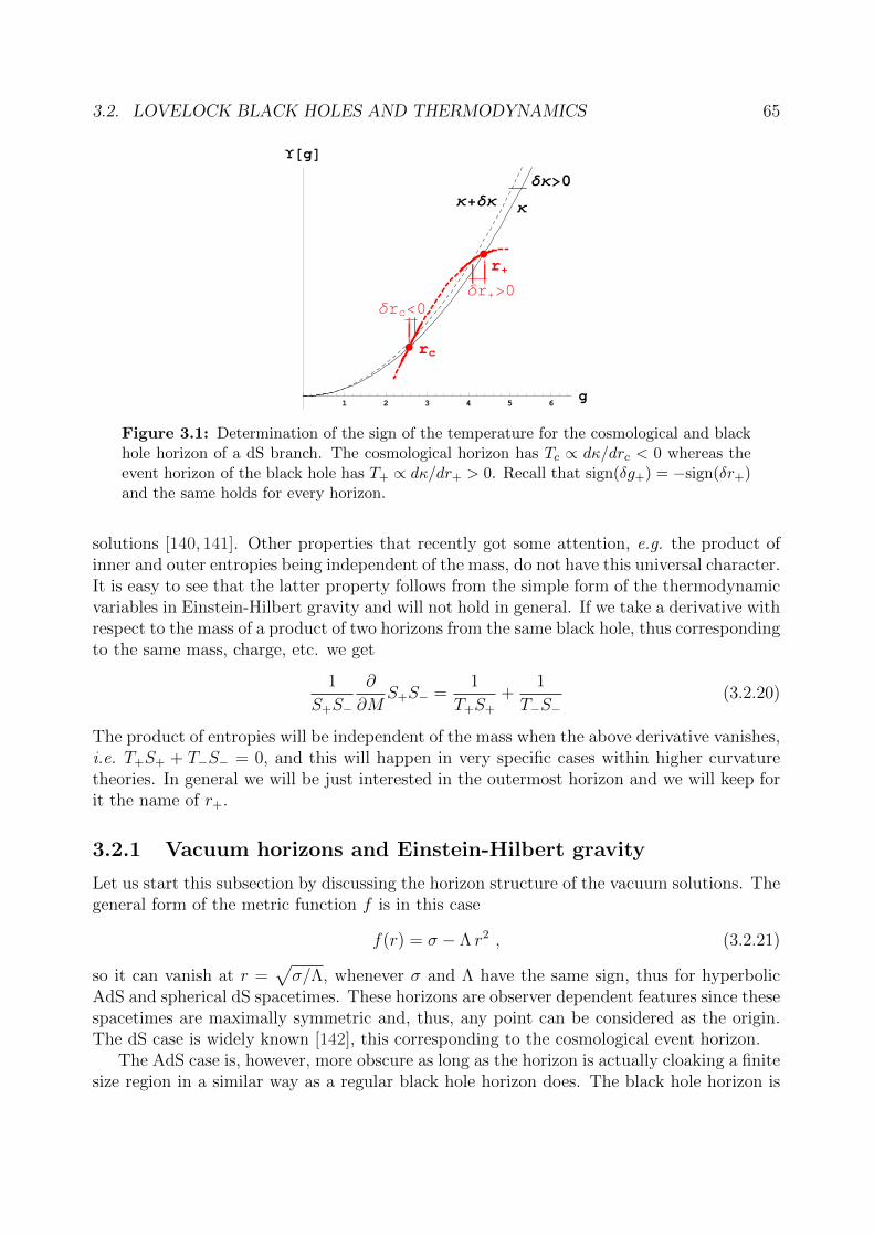
3.2. LOVELOCK BLACK HOLES AND THERMODYNAMICS 65
1 2 3 4 5 6g
U@gD
r+
rc
∆r+>0∆rc<0
ÈÈÈÈ
ÈÈÈ
Κ+∆ΚΚ
∆Κ>0
Figure 3.1: Determination of the sign of the temperature for the cosmological and blackhole horizon of a dS branch. The cosmological horizon has Tc ∝ dκ/drc < 0 whereas theevent horizon of the black hole has T+ ∝ dκ/dr+ > 0. Recall that sign(δg+) = −sign(δr+)and the same holds for every horizon.
solutions [140, 141]. Other properties that recently got some attention, e.g. the product ofinner and outer entropies being independent of the mass, do not have this universal character.It is easy to see that the latter property follows from the simple form of the thermodynamicvariables in Einstein-Hilbert gravity and will not hold in general. If we take a derivative withrespect to the mass of a product of two horizons from the same black hole, thus correspondingto the same mass, charge, etc. we get
1
S+S−
∂
∂MS+S− =
1
T+S+
+1
T−S−(3.2.20)
The product of entropies will be independent of the mass when the above derivative vanishes,i.e. T+S+ + T−S− = 0, and this will happen in very specific cases within higher curvaturetheories. In general we will be just interested in the outermost horizon and we will keep forit the name of r+.
3.2.1 Vacuum horizons and Einstein-Hilbert gravity
Let us start this subsection by discussing the horizon structure of the vacuum solutions. Thegeneral form of the metric function f is in this case
f(r) = σ − Λ r2 , (3.2.21)
so it can vanish at r =√σ/Λ, whenever σ and Λ have the same sign, thus for hyperbolic
AdS and spherical dS spacetimes. These horizons are observer dependent features since thesespacetimes are maximally symmetric and, thus, any point can be considered as the origin.The dS case is widely known [142], this corresponding to the cosmological event horizon.
The AdS case is, however, more obscure as long as the horizon is actually cloaking a finitesize region in a similar way as a regular black hole horizon does. The black hole horizon is

66 CHAPTER 3. BLACK HOLE THERMODYNAMICS
-2 -1 1 2 3 4g
U@gD
Σ=1
Σ=0
Σ=-1c0=1 c0=0 c0=-1
Κ=2
Κ=0.2
ΚNariai
Figure 3.2: Linear polynomial corresponding to the usual EH branch for negative (c0 = 1),zero (c0 = 0) and positive (c0 = −1) cosmological constants (L = 1). The dashed lines
are just κ (g/σ)d−1
2 for d = 5. The solid black line corresponds to the critical value of themass, κNariai = 1/4, for dS black holes with spherical horizon. The crossing of these lineswith the polynomial gives the possible values for g at the horizon and then of r+ (and rc).For σ = 1 and κ > κNariai (or r+ > rNariai), the asymptotically dS branch describes a bigcrunch spacetime (f < 0, ∀r) without horizons.
actually just a deformation of this ‘vacuum’ horizon. This has a problematic interpretationand has led to the proposal that the true ground state for hyperbolic spacetimes is not themassless one, but an extremal negative mass solution [134, 135]. The cosmological horizonof pure dS spacetime has negative temperature, while for the AdS case the temperature ispositive as for a regular black hole horizon.
In order to analyze the horizon structure, let us focus on the asymptotically AdS, dS andflat black holes in Einstein-Hilbert gravity with cosmological constant [135]. We include thissimple case here for completeness and as an illustration of our method. As clearly depictedin figure 3.2, the only case accepting all three distinct topologies without exhibiting nakedsingularities is the asymptotically AdS configuration, the other two cases being well-definedjust for spherical topology. This AdS case, furthermore, has just one horizon for all threetopologies. The asymptotically flat spherical black hole has one event horizon as well. Theasymptotically dS spherical black hole has in general two horizons: One of them is justthe deformation of the cosmological horizon already present in the maximally symmetricsolution, while the other corresponds to the black hole. As the mass increases both horizonsget closer to each other until, for some critical value of the mass, the so-called Nariai mass,
κNariai =2Ld−3
d− 1
(d− 3
d− 1
) d−32
, (3.2.22)
they actually meet (they disappear for masses above that value). The untrapped region,the spacetime as we usually consider it, is comprised between the two horizons and so forthis extremal case it seems to disappear. A proper limiting procedure [143] shows that thegeometry remains perfectly regular as κ → κNariai, and becomes the geometry of the Nariai
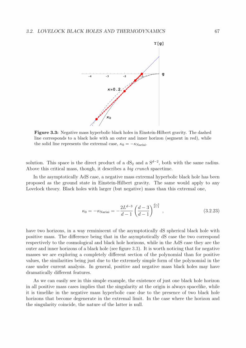
3.2. LOVELOCK BLACK HOLES AND THERMODYNAMICS 67
-4 -3 -2 -1g
U@gDΣ=0
Κ0
Κ=0.2
Figure 3.3: Negative mass hyperbolic black holes in Einstein-Hilbert gravity. The dashedline corresponds to a black hole with an outer and inner horizon (segment in red), whilethe solid line represents the extremal case, κ0 = −κNariai.
solution. This space is the direct product of a dS2 and a Sd−2, both with the same radius.Above this critical mass, though, it describes a big crunch spacetime.
In the asymptotically AdS case, a negative mass extremal hyperbolic black hole has beenproposed as the ground state in Einstein-Hilbert gravity. The same would apply to anyLovelock theory. Black holes with larger (but negative) mass than this extremal one,
κ0 = −κNariai = −2Ld−3
d− 1
(d− 3
d− 1
) d−3d−1
, (3.2.23)
have two horizons, in a way reminiscent of the asymptotically dS spherical black hole withpositive mass. The difference being that in the asymptotically dS case the two correspondrespectively to the cosmological and black hole horizons, while in the AdS case they are theouter and inner horizons of a black hole (see figure 3.3). It is worth noticing that for negativemasses we are exploring a completely different section of the polynomial than for positivevalues, the similarities being just due to the extremely simple form of the polynomial in thecase under current analysis. In general, positive and negative mass black holes may havedramatically different features.
As we can easily see in this simple example, the existence of just one black hole horizonin all positive mass cases implies that the singularity at the origin is always spacelike, whileit is timelike in the negative mass hyperbolic case due to the presence of two black holehorizons that become degenerate in the extremal limit. In the case where the horizon andthe singularity coincide, the nature of the latter is null.
68 CHAPTER 3. BLACK HOLE THERMODYNAMICS
3.2.2 Black hole entropy at extremality
As we have seen in the last section, the vacuum (M = 0) state with hyperbolic topology hasnonzero temperature as it displays a horizon. This is related to the fact that an acceleratedobserver in AdS would see a horizon with temperature related to its acceleration, in a similarmanner as for the Unruh effect in Minkowski space. This makes it difficult to assume thisstate as groundstate, it cannot be considered at arbitrary temperature as it already has one.The alternative is to consider an extremal state instead. For that we have to make somecomments on the special properties of extremal black holes.
There has been some debate (see [144,145] for some recent discussion) about whether theentropy of extremal black holes corresponds to the usual Bekenstein-Hawking (or Wald inmore general cases) or it is simply zero as it seems to indicate the semiclassical calculation[146–148]. Both approaches yield the same result in the non-extremal case, the reason forthis discrepancy at extremality being the qualitative difference in the near horizon topologyin both cases. In the Euclidean section, it has the topology of R2 × Σd−2 for non-extremalblack holes whereas it is R×S1×Σd−2 in the extremal case, effectively removing the horizonfrom the geometry. In the first case regularity of the flat factor forces the Euclidean time tobe identified such that the period is the inverse of the temperature. This introduces a non-trivial temperature dependence on the solution and thus in the Euclidean on-shell action, I,that it is at the origin of the entropy in this semiclassical picture. The entropy is defined as
S =
(β∂
∂β− 1
)I . (3.2.24)
In the extremal case the geometry is regular independently of the period β and the solutiondoes not depend on this parameter either. The action depends on β just because of theintegration of the volume of the time circle, I being just proportional to β. The entropythus vanishes as it can also be explicitly seen from the on-shell action computation. Thenaıve result is
I = β(M − T S
)(3.2.25)
where T = f ′(r+)/4π is the usual expression for the black hole temperature. In the non-extremal case, the regularity of the solution at the horizon requires β = T−1 in such a waythat the β-dependence of the second term cancels and we get
I = βM − S (3.2.26)
as expected. The extremal black hole is different as β and T are unrelated in that case.Actually T = 0 yielding Ie = βM e. The entropy would then vanish for the extremal blackhole.
Some other approaches yield the same form of the Bekenstein or Wald entropy but theyusually rely on extremal limits of near-extremal solutions, whereas in our case we haveassumed that the extremality condition holds a priori. In case we want to consider anyextremal state as ground state for a sector of the theory we will need it to be identified witharbitrary periodicity in Euclidean time. This cannot be done as we take the extremal limitof near-extremal solutions as in that case the temperature would be bound to vanish. We
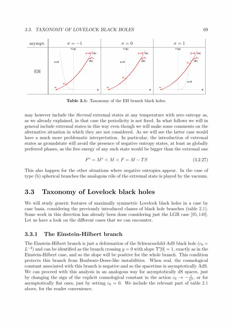
3.3. TAXONOMY OF LOVELOCK BLACK HOLES 69
asympt. σ = −1 σ = 0 σ = 1
EH
g
U@gDr®0
r*
¥
r+
Κ>0
HaL
HbL
g
U@gDr®0
r*
¥
r+
Κ>0
HaL
HbL
g
U@gD
r+
r*
¥
r®0
Κ>0
HaL
HbL
Table 3.1: Taxonomy of the EH branch black holes.
may however include the thermal extremal states at any temperature with zero entropy as,as we already explained, in that case the periodicity is not fixed. In what follows we will ingeneral include extremal states in this way even though we will make some comments on thealternative situation in which they are not considered. As we will see the latter case wouldhave a much more problematic interpretation. In particular, the introduction of extremalstates as groundstate will avoid the presence of negative entropy states, at least as globallypreferred phases, as the free energy of any such state would be bigger than the extremal one
F e = M e < M < F = M − TS (3.2.27)
This also happen for the other situations where negative entropies appear. In the case oftype (b) spherical branches the analogous role of the extremal state is played by the vacuum.
3.3 Taxonomy of Lovelock black holes
We will study generic features of maximally symmetric Lovelock black holes in a case bycase basis, considering the previously introduced classes of black hole branches (table 2.1).Some work in this direction has already been done considering just the LGB case [95, 149].Let us have a look on the different cases that we can encounter.
3.3.1 The Einstein-Hilbert branch
The Einstein-Hilbert branch is just a deformation of the Schwarzschild-AdS black hole (c0 =L−2) and can be identified as the branch crossing g = 0 with slope Υ′[0] = 1, exactly as in theEinstein-Hilbert case, and so the slope will be positive for the whole branch. This conditionprotects this branch from Boulware-Deser-like instabilities. When real, the cosmologicalconstant associated with this branch is negative and so the spacetime is asymptotically AdS.We can proceed with this analysis in an analogous way for asymptotically dS spaces, justby changing the sign of the explicit cosmological constant in the action c0 → − 1
L2 , or forasymptotically flat ones, just by setting c0 = 0. We include the relevant part of table 2.1above, for the reader convenience.
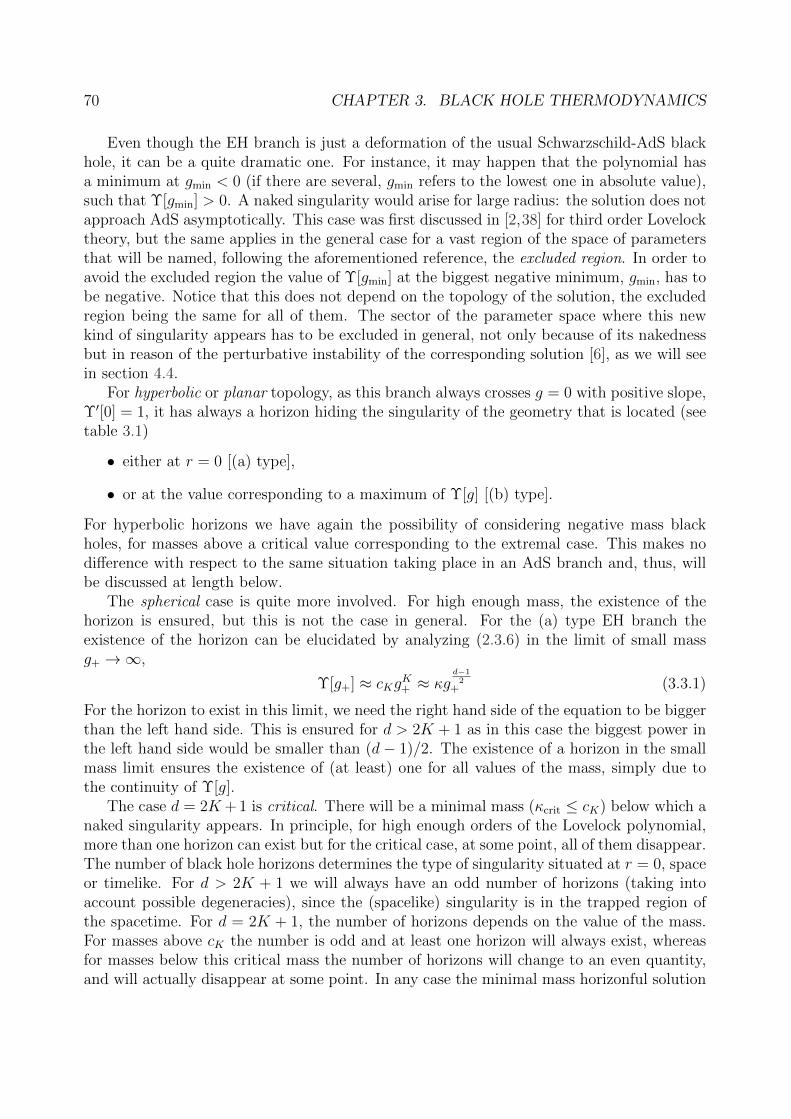
70 CHAPTER 3. BLACK HOLE THERMODYNAMICS
Even though the EH branch is just a deformation of the usual Schwarzschild-AdS blackhole, it can be a quite dramatic one. For instance, it may happen that the polynomial hasa minimum at gmin < 0 (if there are several, gmin refers to the lowest one in absolute value),such that Υ[gmin] > 0. A naked singularity would arise for large radius: the solution does notapproach AdS asymptotically. This case was first discussed in [2,38] for third order Lovelocktheory, but the same applies in the general case for a vast region of the space of parametersthat will be named, following the aforementioned reference, the excluded region. In order toavoid the excluded region the value of Υ[gmin] at the biggest negative minimum, gmin, has tobe negative. Notice that this does not depend on the topology of the solution, the excludedregion being the same for all of them. The sector of the parameter space where this newkind of singularity appears has to be excluded in general, not only because of its nakednessbut in reason of the perturbative instability of the corresponding solution [6], as we will seein section 4.4.
For hyperbolic or planar topology, as this branch always crosses g = 0 with positive slope,Υ′[0] = 1, it has always a horizon hiding the singularity of the geometry that is located (seetable 3.1)
• either at r = 0 [(a) type],
• or at the value corresponding to a maximum of Υ[g] [(b) type].
For hyperbolic horizons we have again the possibility of considering negative mass blackholes, for masses above a critical value corresponding to the extremal case. This makes nodifference with respect to the same situation taking place in an AdS branch and, thus, willbe discussed at length below.
The spherical case is quite more involved. For high enough mass, the existence of thehorizon is ensured, but this is not the case in general. For the (a) type EH branch theexistence of the horizon can be elucidated by analyzing (2.3.6) in the limit of small massg+ →∞,
Υ[g+] ≈ cKgK+ ≈ κg
d−12
+ (3.3.1)
For the horizon to exist in this limit, we need the right hand side of the equation to be biggerthan the left hand side. This is ensured for d > 2K + 1 as in this case the biggest power inthe left hand side would be smaller than (d− 1)/2. The existence of a horizon in the smallmass limit ensures the existence of (at least) one for all values of the mass, simply due tothe continuity of Υ[g].
The case d = 2K+ 1 is critical. There will be a minimal mass (κcrit ≤ cK) below which anaked singularity appears. In principle, for high enough orders of the Lovelock polynomial,more than one horizon can exist but for the critical case, at some point, all of them disappear.The number of black hole horizons determines the type of singularity situated at r = 0, spaceor timelike. For d > 2K + 1 we will always have an odd number of horizons (taking intoaccount possible degeneracies), since the (spacelike) singularity is in the trapped region ofthe spacetime. For d = 2K + 1, the number of horizons depends on the value of the mass.For masses above cK the number is odd and at least one horizon will always exist, whereasfor masses below this critical mass the number of horizons will change to an even quantity,and will actually disappear at some point. In any case the minimal mass horizonful solution
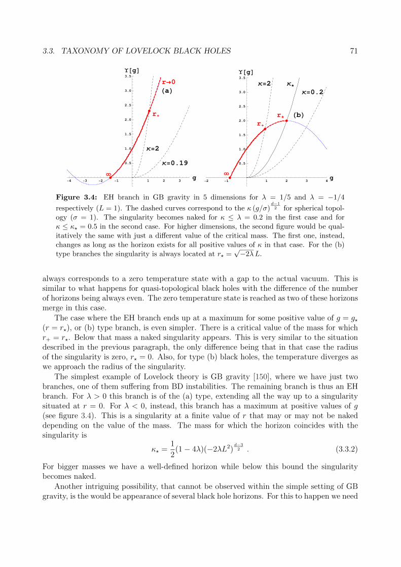
3.3. TAXONOMY OF LOVELOCK BLACK HOLES 71
-4 -3 -2 -1 1 2 3g
0.5
1.0
1.5
2.0
2.5
3.0
3.5
U@gDr®0
¥
r+
Κ=2
Κ=0.19
HaL
-2 -1 1 2 3 4g
0.5
1.0
1.5
2.0
2.5
3.0
3.5
U@gD
r*
¥
r+
Κ=2Κ=0.2
Κ*
HbL
Figure 3.4: EH branch in GB gravity in 5 dimensions for λ = 1/5 and λ = −1/4
respectively (L = 1). The dashed curves correspond to the κ (g/σ)d−1
2 for spherical topol-ogy (σ = 1). The singularity becomes naked for κ ≤ λ = 0.2 in the first case and forκ ≤ κ? = 0.5 in the second case. For higher dimensions, the second figure would be qual-itatively the same with just a different value of the critical mass. The first one, instead,changes as long as the horizon exists for all positive values of κ in that case. For the (b)type branches the singularity is always located at r? =
√−2λL.
always corresponds to a zero temperature state with a gap to the actual vacuum. This issimilar to what happens for quasi-topological black holes with the difference of the numberof horizons being always even. The zero temperature state is reached as two of these horizonsmerge in this case.
The case where the EH branch ends up at a maximum for some positive value of g = g?(r = r?), or (b) type branch, is even simpler. There is a critical value of the mass for whichr+ = r?. Below that mass a naked singularity appears. This is very similar to the situationdescribed in the previous paragraph, the only difference being that in that case the radiusof the singularity is zero, r? = 0. Also, for type (b) black holes, the temperature diverges aswe approach the radius of the singularity.
The simplest example of Lovelock theory is GB gravity [150], where we have just twobranches, one of them suffering from BD instabilities. The remaining branch is thus an EHbranch. For λ > 0 this branch is of the (a) type, extending all the way up to a singularitysituated at r = 0. For λ < 0, instead, this branch has a maximum at positive values of g(see figure 3.4). This is a singularity at a finite value of r that may or may not be nakeddepending on the value of the mass. The mass for which the horizon coincides with thesingularity is
κ? =1
2(1− 4λ)(−2λL2)
d−32 . (3.3.2)
For bigger masses we have a well-defined horizon while below this bound the singularitybecomes naked.
Another intriguing possibility, that cannot be observed within the simple setting of GBgravity, is the would be appearance of several black hole horizons. For this to happen we need
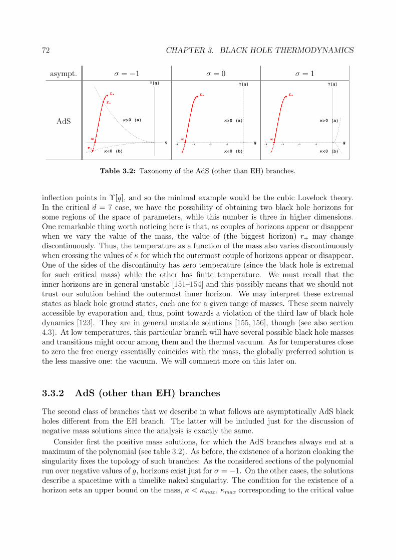
72 CHAPTER 3. BLACK HOLE THERMODYNAMICS
asympt. σ = −1 σ = 0 σ = 1
AdS
g
U@gD
¥
r+
r+
r*
Κ<0 HbL
Κ>0 HaL
-4 -3 -2 -1g
U@gD
¥
r*
Κ<0 HbL
Κ>0 HaL
-4 -3 -2 -1g
U@gD
¥
r*
Κ<0 HbL
Κ>0 HaL
Table 3.2: Taxonomy of the AdS (other than EH) branches.
inflection points in Υ[g], and so the minimal example would be the cubic Lovelock theory.In the critical d = 7 case, we have the possibility of obtaining two black hole horizons forsome regions of the space of parameters, while this number is three in higher dimensions.One remarkable thing worth noticing here is that, as couples of horizons appear or disappearwhen we vary the value of the mass, the value of (the biggest horizon) r+ may changediscontinuously. Thus, the temperature as a function of the mass also varies discontinuouslywhen crossing the values of κ for which the outermost couple of horizons appear or disappear.One of the sides of the discontinuity has zero temperature (since the black hole is extremalfor such critical mass) while the other has finite temperature. We must recall that theinner horizons are in general unstable [151–154] and this possibly means that we should nottrust our solution behind the outermost inner horizon. We may interpret these extremalstates as black hole ground states, each one for a given range of masses. These seem naivelyaccessible by evaporation and, thus, point towards a violation of the third law of black holedynamics [123]. They are in general unstable solutions [155, 156], though (see also section4.3). At low temperatures, this particular branch will have several possible black hole massesand transitions might occur among them and the thermal vacuum. As for temperatures closeto zero the free energy essentially coincides with the mass, the globally preferred solution isthe less massive one: the vacuum. We will comment more on this later on.
3.3.2 AdS (other than EH) branches
The second class of branches that we describe in what follows are asymptotically AdS blackholes different from the EH branch. The latter will be included just for the discussion ofnegative mass solutions since the analysis is exactly the same.
Consider first the positive mass solutions, for which the AdS branches always end at amaximum of the polynomial (see table 3.2). As before, the existence of a horizon cloaking thesingularity fixes the topology of such branches: As the considered sections of the polynomialrun over negative values of g, horizons exist just for σ = −1. On the other cases, the solutionsdescribe a spacetime with a timelike naked singularity. The condition for the existence of ahorizon sets an upper bound on the mass, κ < κmax, κmax corresponding to the critical value
3.3. TAXONOMY OF LOVELOCK BLACK HOLES 73
-6 -4 -2 2g
U@gD
Σ=1
Σ=0
Σ=-1
Κmax
Κ1
Κ2
Figure 3.5: Qualitative representation of (positive mass) AdS branches. The blue andred branches will be referred to as type (b1) and (b2) respectively, when considered fornegative masses. The green one is an excluded branch. There are asymptotically AdSmassive black holes for κ < κmax (red branch), otherwise the geometry displays a nakedsingularity.
for which the radius of the horizon coincide with that of the singularity (r+ = rmax), i.e.,
κmax = rd−1max Υ[gmax] . (3.3.3)
When we encountered a naked singularity with positive mass in the Einstein-Hilberttheory, it corresponded to the low mass limit of a multi-horizon black hole (below a givenmass, the two horizons merge and disappear altogether, leaving the singularity naked). Thecase here is somehow different as the black hole horizon cannot degenerate as we increase themass approaching the critical value. Thereby, the solution infinitesimally close to the criticalone has nonzero temperature, diverging as we approach the bound. This is more reminiscentof the low mass limit of Schwarzschild black holes (ultimately leading to a regular geometry)than of the usual naked singularities in Einstein-Hilbert gravity. It is also similar to whathappens for type (b) spherical black holes.
For negative mass solutions, the analysis of the existence of black hole horizons and itsnumber is more involved. The main qualitative feature is the possibility of having a minimumof the polynomial associated to the branch under analysis (see blue and red branches in figure3.5 for instance). We will refer to the case without such minimum (blue branch) as type (b1)solution and as type (b2) for the other one (red branch). The structure of horizons and thetype of singularity will differ in both types of branches.
When d = 2K + 1 and the branch we are considering is of (b1) type, there is a minimalmass for which, instead of an extremal regular spacetime with a degenerate horizon, wehave a naked singularity (see figure 3.6). The temperature also vanishes asymptotically aswe decrease the mass. We will not comment further on these kind of solutions as they aregravitationally unstable against perturbations [8].
In case we have a well-defined extremal negative mass black hole, we always have at leasttwo horizons for (b1) type branches and d > 2K + 1, as we depart from extremality. For(b2) type branches, however, the inner horizon disappears when its radius coincides with the
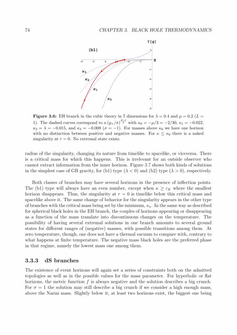
74 CHAPTER 3. BLACK HOLE THERMODYNAMICS
-6 -5 -4 -3 -2 -1g
-5
-4
-3
-2
-1
1
U@gD
Κ1
Κ2
Κ0
Κ3
Hb1L
Figure 3.6: EH branch in the cubic theory in 7 dimensions for λ = 0.4 and µ = 0.2 (L =
1). The dashed curves correspond to κ (g+/σ)d−1
2 with κ0 = −µ/3 = −2/30, κ1 = −0.022,κ2 = λ = −0.015, and κ3 = −0.008 (σ = −1). For masses above κ0 we have one horizonwith no distinction between positive and negative masses. For κ ≤ κ0 there is a nakedsingularity at r = 0. No extremal state exists.
radius of the singularity, changing its nature from timelike to spacelike, or viceversa. Thereis a critical mass for which this happens. This is irrelevant for an outside observer whocannot extract information from the inner horizon. Figure 3.7 shows both kinds of solutionsin the simplest case of GB gravity, for (b1) type (λ < 0) and (b2) type (λ > 0), respectively.
Both classes of branches may have several horizons in the presence of inflection points.The (b1) type will always have an even number, except when κ ≥ cK where the smallesthorizon disappears. Thus, the singularity at r = 0 is timelike below this critical mass andspacelike above it. The same change of behavior for the singularity appears in the other typeof branches with the critical mass being set by the minimum, κ?. In the same way as describedfor spherical black holes in the EH branch, the couples of horizons appearing or disappearingas a function of the mass translate into discontinuous changes on the temperature. Thepossibility of having several extremal solutions in one branch amounts to several groundstates for different ranges of (negative) masses, with possible transitions among them. Atzero temperature, though, one does not have a thermal vacuum to compare with, contrary towhat happens at finite temperature. The negative mass black holes are the preferred phasein that regime, namely the lowest mass one among them.
3.3.3 dS branches
The existence of event horizons will again set a series of constraints both on the admittedtopologies as well as in the possible values for the mass parameter. For hyperbolic or flathorizons, the metric function f is always negative and the solution describes a big crunch.For σ = 1 the solution may still describe a big crunch if we consider a high enough mass,above the Nariai mass. Slightly below it, at least two horizons exist, the biggest one being
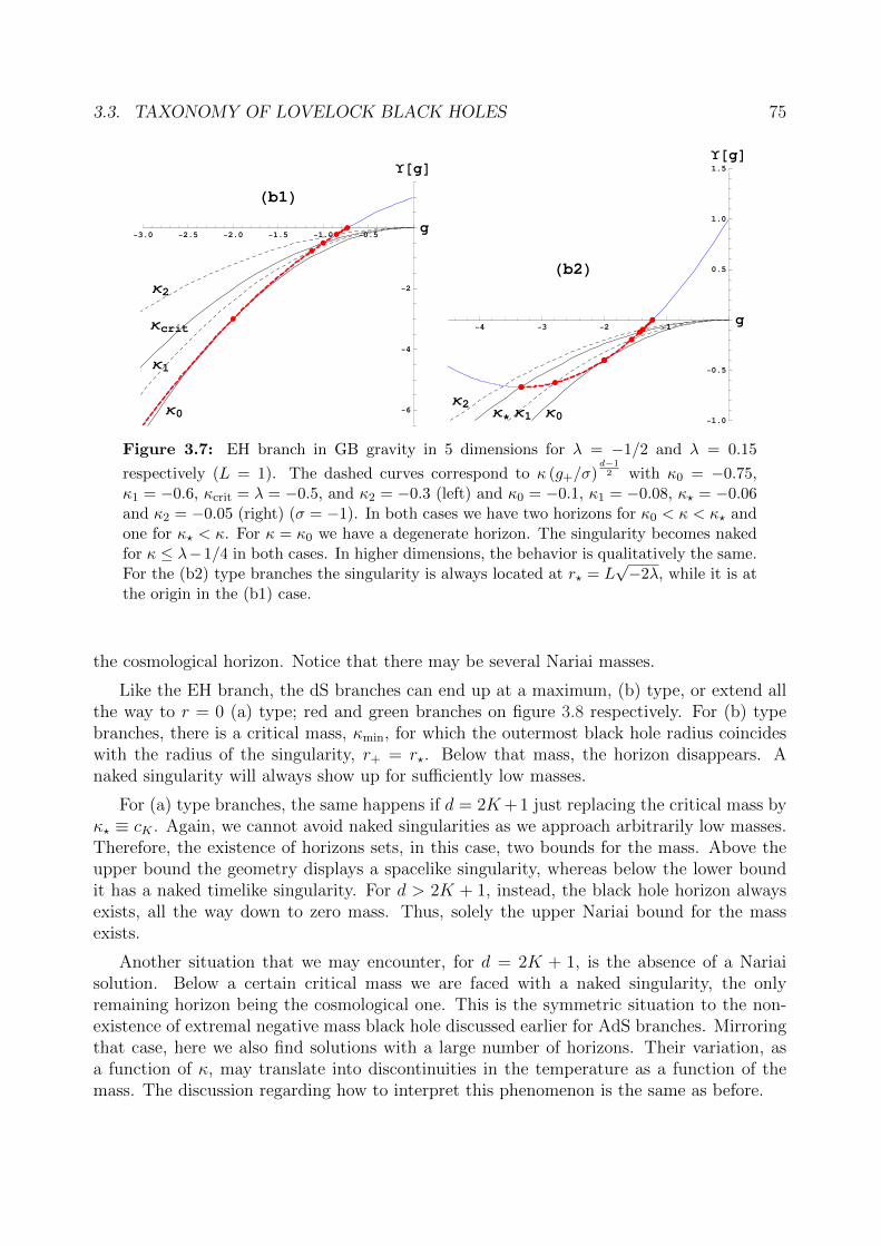
3.3. TAXONOMY OF LOVELOCK BLACK HOLES 75
-3.0 -2.5 -2.0 -1.5 -1.0 -0.5g
-6
-4
-2
U@gDr* r+
Κ1
Κ2
Κcrit
Κ0
Hb1L
-4 -3 -2 -1g
-1.0
-0.5
0.5
1.0
1.5
U@gD
Κ1Κ2
Κ0Κ*
Hb2L
Figure 3.7: EH branch in GB gravity in 5 dimensions for λ = −1/2 and λ = 0.15
respectively (L = 1). The dashed curves correspond to κ (g+/σ)d−1
2 with κ0 = −0.75,κ1 = −0.6, κcrit = λ = −0.5, and κ2 = −0.3 (left) and κ0 = −0.1, κ1 = −0.08, κ? = −0.06and κ2 = −0.05 (right) (σ = −1). In both cases we have two horizons for κ0 < κ < κ? andone for κ? < κ. For κ = κ0 we have a degenerate horizon. The singularity becomes nakedfor κ ≤ λ−1/4 in both cases. In higher dimensions, the behavior is qualitatively the same.For the (b2) type branches the singularity is always located at r? = L
√−2λ, while it is at
the origin in the (b1) case.
the cosmological horizon. Notice that there may be several Nariai masses.
Like the EH branch, the dS branches can end up at a maximum, (b) type, or extend allthe way to r = 0 (a) type; red and green branches on figure 3.8 respectively. For (b) typebranches, there is a critical mass, κmin, for which the outermost black hole radius coincideswith the radius of the singularity, r+ = r?. Below that mass, the horizon disappears. Anaked singularity will always show up for sufficiently low masses.
For (a) type branches, the same happens if d = 2K+1 just replacing the critical mass byκ? ≡ cK . Again, we cannot avoid naked singularities as we approach arbitrarily low masses.Therefore, the existence of horizons sets, in this case, two bounds for the mass. Above theupper bound the geometry displays a spacelike singularity, whereas below the lower boundit has a naked timelike singularity. For d > 2K + 1, instead, the black hole horizon alwaysexists, all the way down to zero mass. Thus, solely the upper Nariai bound for the massexists.
Another situation that we may encounter, for d = 2K + 1, is the absence of a Nariaisolution. Below a certain critical mass we are faced with a naked singularity, the onlyremaining horizon being the cosmological one. This is the symmetric situation to the non-existence of extremal negative mass black hole discussed earlier for AdS branches. Mirroringthat case, here we also find solutions with a large number of horizons. Their variation, asa function of κ, may translate into discontinuities in the temperature as a function of themass. The discussion regarding how to interpret this phenomenon is the same as before.
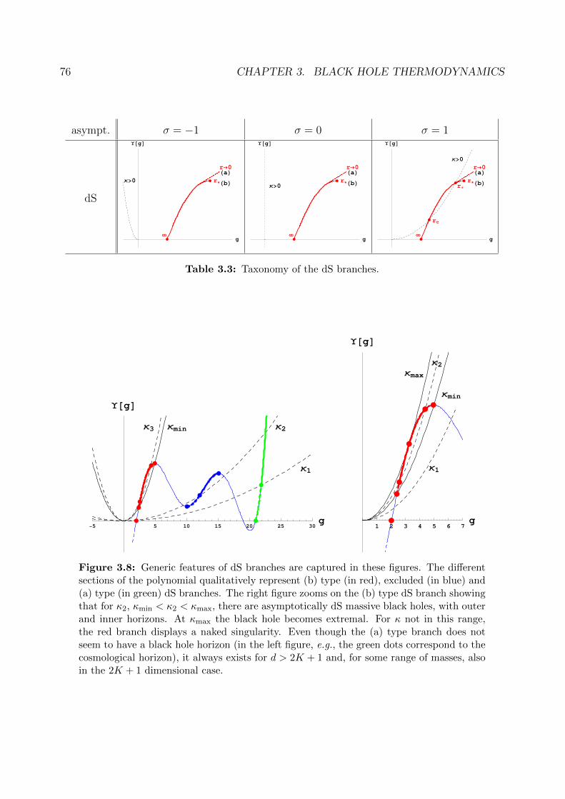
76 CHAPTER 3. BLACK HOLE THERMODYNAMICS
asympt. σ = −1 σ = 0 σ = 1
dS
g
U@gD
¥
r*
r®0
Κ>0HaLHbL
g
U@gD
¥
r*
r®0
Κ>0
HaLHbL
g
U@gD
¥
r*
rc
r+
r®0Κ>0
HaLHbL
Table 3.3: Taxonomy of the dS branches.
-5 5 10 15 20 25 30g
U@gDΚ3 Κmin Κ2
Κ1
1 2 3 4 5 6 7g
U@gD
Κmax
Κmin
Κ2
Κ1
Figure 3.8: Generic features of dS branches are captured in these figures. The differentsections of the polynomial qualitatively represent (b) type (in red), excluded (in blue) and(a) type (in green) dS branches. The right figure zooms on the (b) type dS branch showingthat for κ2, κmin < κ2 < κmax, there are asymptotically dS massive black holes, with outerand inner horizons. At κmax the black hole becomes extremal. For κ not in this range,the red branch displays a naked singularity. Even though the (a) type branch does notseem to have a black hole horizon (in the left figure, e.g., the green dots correspond to thecosmological horizon), it always exists for d > 2K + 1 and, for some range of masses, alsoin the 2K + 1 dimensional case.
3.4. HEAT CAPACITY AND LOCAL THERMODYNAMIC STABILITY 77
3.4 Heat capacity and local thermodynamic stability
The details of the solutions and the behavior of their associated thermodynamic quantitiesstrongly depend on the particular case under consideration. Therefore, a general thermody-namic analysis is cumbersome. However, once we have described the qualitative features ofthe different branches of solutions, much and very interesting information can be extracted,most of it arising as universal features of these black hole solutions.
For positive mass black holes, the sign of the heat capacity on a BD stable branch,because of (3.2.18), depends just on
dT
dr+
= −g+
2π
[(d− 2)− d− 1
2
Υ[g+]
g+Υ′[g+]
(1 + 2g+
Υ′′[g+]
Υ′[g+]
)], (3.4.1)
where the second term (in brackets) seems to be related to the potential felt by perturbationsin the shear channel [5]. We did not manage to check classical stability in full generality,but in the regimes of high and low masses. This should not be confused with the stabilityanalysis focusing on perturbations of the black hole solutions that will be treated in the nextchapter. Earlier relevant works on this include [157–163]).
We will just consider solutions possessing event horizons, since they are the only oneswith associated thermodynamic variables. Then, taking into account our earlier discussion(see table 2.1), we will have to deal with hyperbolic AdS branches; hyperbolic, flat andspherical EH branches and spherical dS branches, classified in different subclasses.
3.4.1 Black holes in the EH branch
The simplest case to analyze is that of toroidal or planar black holes in the EH branch.The thermodynamic variables, in this case, do not receive any correction from the highercurvature terms in the action and the expression reduces to the usual formula of Einstein-Hilbert gravity,
dT
dr+
=d− 1
4πL2. (3.4.2)
This expression is positive. Therefore, these black holes are locally thermodynamically stablefor all values of the mass.
For the EH branch, the only one admitting all three topologies, the situation is exactlythe same for σ = ±1 in the large mass limit. The value of g at the horizon, g+ = σ/r2
+,asymptotically approaches zero from both sides, and the formulas reproduce the planar case.Einstein-Hilbert gravity captures the universal thermodynamic description of Lovelock blackholes with large enough mass. It does not capture other features in this regime. For instance,those related to the stability and causality preserving properties of the solutions [2, 3, 38].EH branch’s black holes in this regime are then always stable.
This is also the case for a special class of (maximally degenerated) Lovelock theorieswhose analysis is not considered in the present article. Those theories admit a single (EH-)branch of black holes [164]. The results there also coincide with the generic analysis forspherical black holes presented here.
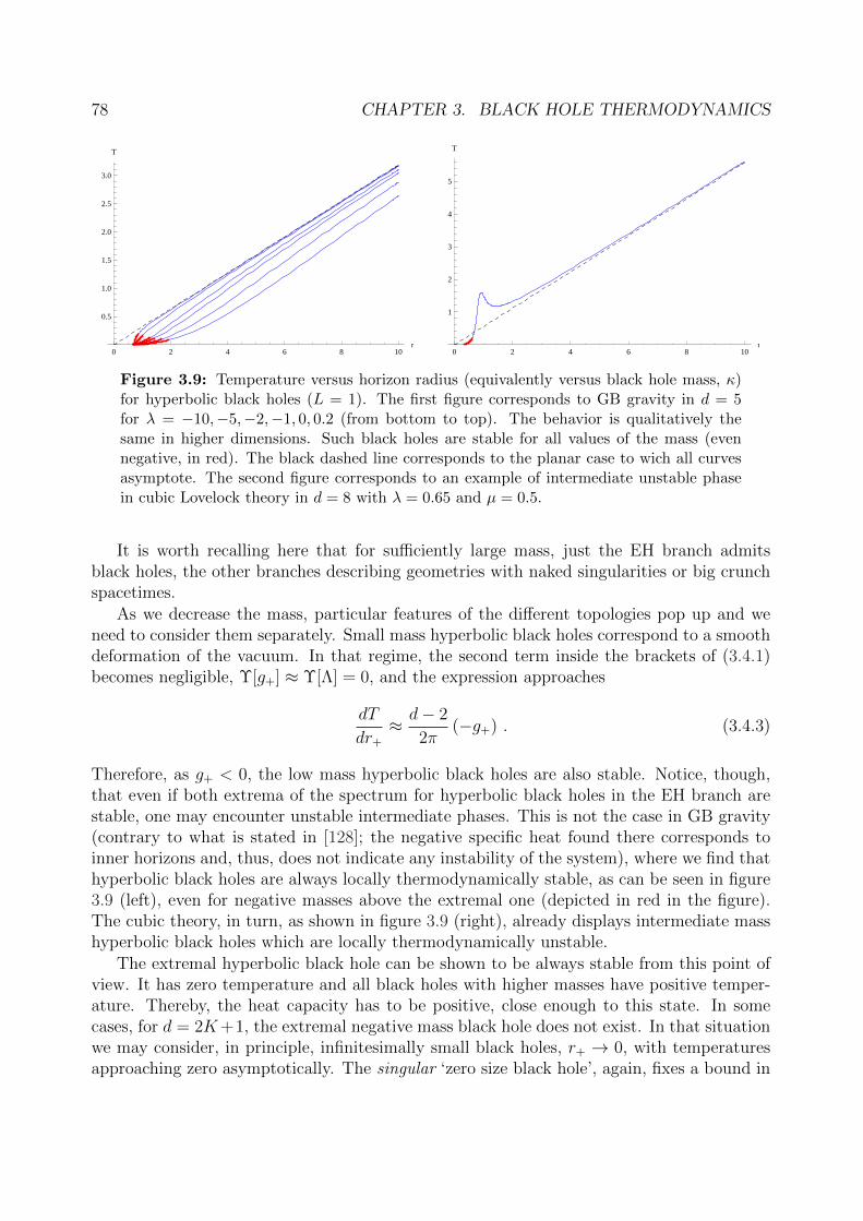
78 CHAPTER 3. BLACK HOLE THERMODYNAMICS
0 2 4 6 8 10r
0.5
1.0
1.5
2.0
2.5
3.0
T
0 2 4 6 8 10r
1
2
3
4
5
T
Figure 3.9: Temperature versus horizon radius (equivalently versus black hole mass, κ)for hyperbolic black holes (L = 1). The first figure corresponds to GB gravity in d = 5for λ = −10,−5,−2,−1, 0, 0.2 (from bottom to top). The behavior is qualitatively thesame in higher dimensions. Such black holes are stable for all values of the mass (evennegative, in red). The black dashed line corresponds to the planar case to wich all curvesasymptote. The second figure corresponds to an example of intermediate unstable phasein cubic Lovelock theory in d = 8 with λ = 0.65 and µ = 0.5.
It is worth recalling here that for sufficiently large mass, just the EH branch admitsblack holes, the other branches describing geometries with naked singularities or big crunchspacetimes.
As we decrease the mass, particular features of the different topologies pop up and weneed to consider them separately. Small mass hyperbolic black holes correspond to a smoothdeformation of the vacuum. In that regime, the second term inside the brackets of (3.4.1)becomes negligible, Υ[g+] ≈ Υ[Λ] = 0, and the expression approaches
dT
dr+
≈ d− 2
2π(−g+) . (3.4.3)
Therefore, as g+ < 0, the low mass hyperbolic black holes are also stable. Notice, though,that even if both extrema of the spectrum for hyperbolic black holes in the EH branch arestable, one may encounter unstable intermediate phases. This is not the case in GB gravity(contrary to what is stated in [128]; the negative specific heat found there corresponds toinner horizons and, thus, does not indicate any instability of the system), where we find thathyperbolic black holes are always locally thermodynamically stable, as can be seen in figure3.9 (left), even for negative masses above the extremal one (depicted in red in the figure).The cubic theory, in turn, as shown in figure 3.9 (right), already displays intermediate masshyperbolic black holes which are locally thermodynamically unstable.
The extremal hyperbolic black hole can be shown to be always stable from this point ofview. It has zero temperature and all black holes with higher masses have positive temper-ature. Thereby, the heat capacity has to be positive, close enough to this state. In somecases, for d = 2K+1, the extremal negative mass black hole does not exist. In that situationwe may consider, in principle, infinitesimally small black holes, r+ → 0, with temperaturesapproaching zero asymptotically. The singular ‘zero size black hole’, again, fixes a bound in
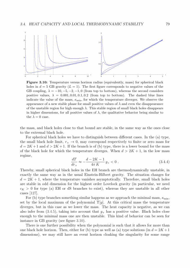
3.4. HEAT CAPACITY AND LOCAL THERMODYNAMIC STABILITY 79
0 2 4 6 8 10r
2
4
6
8
T
0 1 2 3 4 5r
0.5
1.0
1.5
T
Figure 3.10: Temperature versus horizon radius (equivalently, mass) for spherical blackholes in d = 5 GB gravity (L = 1). The first figure corresponds to negative values of theGB coupling, λ = −10,−5,−2,−1, 0 (from top to bottom), whereas the second considerspositive values, λ = 0.001, 0.01, 0.1, 0.2 (from top to bottom). The dashed blue linesindicate the value of the mass, κmin, for which the temperature diverges. We observe theappearance of a new stable phase for small positive values of λ and even the disappearanceof the unstable region for high enough λ. This stable region of small black holes disappearsin higher dimensions, for all positive values of λ, the qualitative behavior being similar tothe λ = 0 case.
the mass, and black holes close to that bound are stable, in the same way as the ones closeto the extremal black hole.
For spherical black holes we have to distinguish between different cases. In the (a) type,the small black hole limit, r+ → 0, may correspond respectively to finite or zero mass ford = 2K+ 1 and d > 2K+ 1. If the branch is of (b) type, there is a lower bound for the massof the black hole for which the temperature diverges. When d > 2K + 1, in the low massregime,
dT
dr+
≈ −d− 2K − 1
4πKg+ < 0 . (3.4.4)
Thereby, small spherical black holes in the EH branch are thermodynamically unstable, inexactly the same way as in the usual Einstein-Hilbert gravity. The situation changes ford = 2K + 1, where the temperature vanishes asymptotically. Therefore, small black holesare stable in odd dimension for the highest order Lovelock gravity (in particular, we needcK > 0 for type (a) EH or dS branches to exist), whereas they are unstable in all othercases [127].
For (b) type branches something similar happens as we approach the minimal mass, κmin,set by the local maximum of the polynomial Υ[g]. At this critical mass the temperaturediverges, but in this case as we lower the mass. The heat capacity is negative, as we canalso infer from (3.4.5), taking into account that g+ has a positive value. Black holes closeenough to the minimal mass one are then unstable. This kind of behavior can be seen forinstance in GB gravity (see figure 3.10).
There is one further possibility when the polynomial is such that it allows for more thanone black hole horizon. Then, either for (b) type as well as (a) type solutions (in d = 2K+ 1dimensions), we may still have an event horizon cloaking the singularity for some range
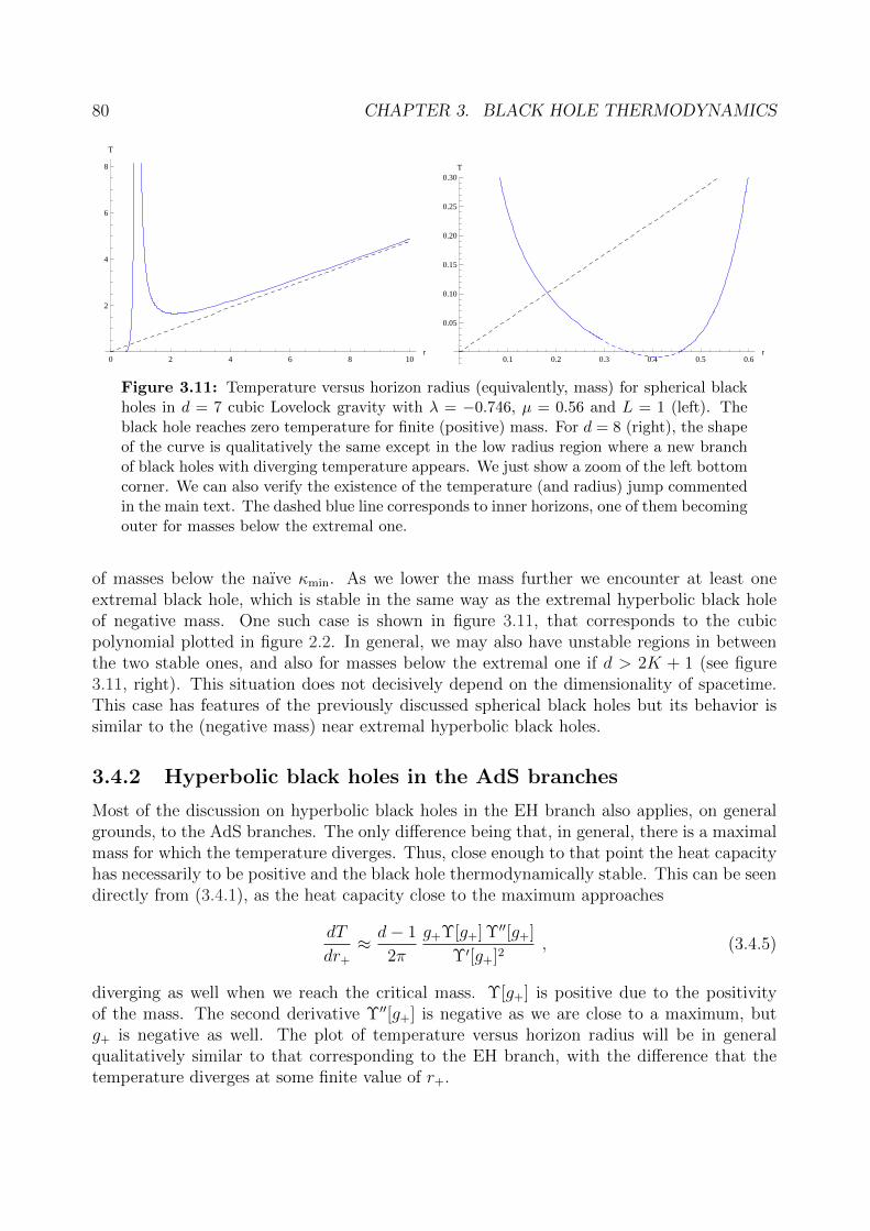
80 CHAPTER 3. BLACK HOLE THERMODYNAMICS
0 2 4 6 8 10r
2
4
6
8
T
0.1 0.2 0.3 0.4 0.5 0.6r
0.05
0.10
0.15
0.20
0.25
0.30T
Figure 3.11: Temperature versus horizon radius (equivalently, mass) for spherical blackholes in d = 7 cubic Lovelock gravity with λ = −0.746, µ = 0.56 and L = 1 (left). Theblack hole reaches zero temperature for finite (positive) mass. For d = 8 (right), the shapeof the curve is qualitatively the same except in the low radius region where a new branchof black holes with diverging temperature appears. We just show a zoom of the left bottomcorner. We can also verify the existence of the temperature (and radius) jump commentedin the main text. The dashed blue line corresponds to inner horizons, one of them becomingouter for masses below the extremal one.
of masses below the naıve κmin. As we lower the mass further we encounter at least oneextremal black hole, which is stable in the same way as the extremal hyperbolic black holeof negative mass. One such case is shown in figure 3.11, that corresponds to the cubicpolynomial plotted in figure 2.2. In general, we may also have unstable regions in betweenthe two stable ones, and also for masses below the extremal one if d > 2K + 1 (see figure3.11, right). This situation does not decisively depend on the dimensionality of spacetime.This case has features of the previously discussed spherical black holes but its behavior issimilar to the (negative mass) near extremal hyperbolic black holes.
3.4.2 Hyperbolic black holes in the AdS branches
Most of the discussion on hyperbolic black holes in the EH branch also applies, on generalgrounds, to the AdS branches. The only difference being that, in general, there is a maximalmass for which the temperature diverges. Thus, close enough to that point the heat capacityhas necessarily to be positive and the black hole thermodynamically stable. This can be seendirectly from (3.4.1), as the heat capacity close to the maximum approaches
dT
dr+
≈ d− 1
2π
g+Υ[g+] Υ′′[g+]
Υ′[g+]2, (3.4.5)
diverging as well when we reach the critical mass. Υ[g+] is positive due to the positivityof the mass. The second derivative Υ′′[g+] is negative as we are close to a maximum, butg+ is negative as well. The plot of temperature versus horizon radius will be in generalqualitatively similar to that corresponding to the EH branch, with the difference that thetemperature diverges at some finite value of r+.
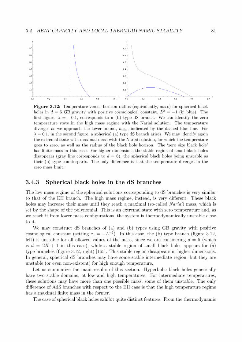
3.4. HEAT CAPACITY AND LOCAL THERMODYNAMIC STABILITY 81
0.0 0.2 0.4 0.6 0.8 1.0r
0.1
0.2
0.3
0.4
0.5
0.6
0.7
T
0.0 0.2 0.4 0.6 0.8 1.0r
0.1
0.2
0.3
0.4
0.5
0.6
0.7
T
Figure 3.12: Temperature versus horizon radius (equivalently, mass) for spherical blackholes in d = 5 GB gravity with positive cosmological constant, L2 = −1 (in blue). Thefirst figure, λ = −0.1, corresponds to a (b) type dS branch. We can identify the zerotemperature state in the high mass regime with the Nariai solution. The temperaturediverges as we approach the lower bound, κmin, indicated by the dashed blue line. Forλ = 0.1, in the second figure, a spherical (a) type dS branch arises. We may identify againthe extremal state with maximal mass with the Nariai solution, for which the temperaturegoes to zero, as well as the radius of the black hole horizon. The ‘zero size black hole’has finite mass in this case. For higher dimensions the stable region of small black holesdisappears (gray line corresponds to d = 6), the spherical black holes being unstable astheir (b) type counterparts. The only difference is that the temperature diverges in thezero mass limit.
3.4.3 Spherical black holes in the dS branches
The low mass regime of the spherical solutions corresponding to dS branches is very similarto that of the EH branch. The high mass regime, instead, is very different. These blackholes may increase their mass until they reach a maximal (so-called Nariai) mass, which isset by the shape of the polynomial. This is an extremal state with zero temperature and, aswe reach it from lower mass configurations, the system is thermodynamically unstable closeto it.
We may construct dS branches of (a) and (b) types using GB gravity with positivecosmological constant (setting c0 = −L−2). In this case, the (b) type branch (figure 3.12,left) is unstable for all allowed values of the mass, since we are considering d = 5 (whichis d = 2K + 1 in this case), while a stable region of small black holes appears for (a)type branches (figure 3.12, right) [165]. This stable region disappears in higher dimensions.In general, spherical dS branches may have some stable intermediate region, but they areunstable (or even non-existent) for high enough temperature.
Let us summarize the main results of this section. Hyperbolic black holes genericallyhave two stable domains, at low and high temperatures. For intermediate temperatures,these solutions may have more than one possible mass, some of them unstable. The onlydifference of AdS branches with respect to the EH case is that the high temperature regimehas a maximal finite mass in the former.
The case of spherical black holes exhibit quite distinct features. From the thermodynamic
82 CHAPTER 3. BLACK HOLE THERMODYNAMICS
point of view, we may distinguish those situations where there is, or there is not, a minimaltemperature, Tmin, for the black holes to exist. In the former case, we do not reach anyextremal black hole, neither in the low mass, nor in the high mass regimes. In the case ofthe EH branch, for T < Tmin, only the thermal vacuum may exist whereas, for high enoughtemperatures, a black hole may exist with two very different masses, one close to κmin (whichis unstable) and one very high (stable). For intermediate temperatures close to Tmin, we mayin principle encounter several stable and/or unstable black holes. In the latter case, instead,black hole solutions exist for the whole range of temperatures, except in the case where a dSbranch reaches an extremal state at low as well as at high masses. For the EH branch, in thissituation, we have two stable phases again, one in the low and one in the high temperatureregimes. At intermediate temperatures, the black hole may have several possible masses,some of them unstable.
3.5 Hawking-Page-like phase transitions
The existence of unstable phases, as well as the several possible black hole solutions atthe same temperature, suggest the occurrence of Hawking-Page-like phase transitions, asalready observed in the case of LGB gravity [130, 138]. These phase transitions should bealso relevant when studying the physics of the dual CFT plasma. In order to analyze thiswe need to discuss the global stability of the solutions. Any system in thermal equilibriumwith an infinite heat reservoir (and thus at constant temperature) will be described by thecanonical ensemble, whose relevant thermodynamic potential is the Helmholtz free energy,F . The preferred, and so globally stable, solution is the one that minimizes F . For instance,the free energy of the black hole solution calculated in (3.2.9), is the free energy with respectto the vacuum solution, except for the hyperbolic case where the finite ground state freeenergy (its mass) must be subtracted. Therefore, the sign of the free energy determineswhich solution is globally preferred at any given temperature, the appropriate black hole (ifseveral are possible) or a thermal bath for the groundstate (vacuum or extremal).
The general analysis is, again, hard and not very enlightening. We will just concentratein showing general features of these black hole solutions without entering into the detailsof the different cases. We will consider the same regimes analyzed for the local stability, asthere we can easily find the expression for the free energy. In the planar case the analysis isvery simple since the free energy reads
F = − Vd−2
16πG
rd−1+
L2. (3.5.1)
The black hole is then always the preferred solution, as indicated by the negative sign of thefree energy, and no phase transitions occur. This will be the situation in the large mass limitof the other topologies in the EH branch. As for large enough r+ the free energy may be aslarge as one wants, ambiguities on the reference background do not matter in this limit.
3.5. HAWKING-PAGE-LIKE PHASE TRANSITIONS 83
3.5.1 Spherical black holes
For spherical black holes, we will restrict our discussion to the two most generic situations.For the EH branch, we will consider separately the case of having a stable low temperaturephase (as in d = 5 GB gravity with positive λ), and the case where a minimal temperatureis needed for black hole solutions to exist. The second case is the analogue of the usualsituation in Einstein-Hilbert gravity. At low temperatures, the thermal vacuum can beconsidered as the globally stable solution whereas, for higher temperatures, two or moreblack hole solutions are possible. For high enough temperature just two of them remain.The small one has always positive free energy. For an (a) type branch,
F =(d− 2)Vd−2
16πG
rd−2K−1+
d− 2KcK , (3.5.2)
whereas for the (b) type case the temperature diverges as we approach the maximum g+ →g?, and the free energy is F ≈ −TS. Then, for positive entropy, the small black hole solutionhas negative free energy and is stable against the vacuum. However, it is not the minimumof the free energy since the big black hole has always a lower one. This is quite easy to see byrealizing that the small black hole entropy goes to a constant as we approach g? whereas theentropy grows indefinitely for big black holes, since they approach the planar limit. Thus,the small black holes are not just locally but also globally unstable.
The big black holes have, in general, negative free energy. We have then a Hawking-Page-like phase transition, from the thermal vacuum at low temperatures to big black holes athigh temperatures. The difference with respect to the Einstein-Hilbert case is that we mayhave several black holes at intermediate temperatures, with either sign of the free energy.For ranges of temperature where several black holes have negative free energy, transitionsamong them may happen, the globally preferred solution being the one with the lowest freeenergy. This would be an example of a new kind of phase transition, different from theHawking-Page one, where one of the phases is always the thermal vacuum.
If the EH branch has stable low temperature black holes, i.e., for (a) type in d = 2K+ 1,these are globally unstable as indicated by their positive free energy that asymptotes aconstant when r+ → 0,
F =(d− 2)Vd−2
16πGcK , (3.5.3)
actually to the mass as both the entropy and temperature vanish in this limit. This isexactly equal to the earlier formula (3.5.2) for the given dimension. The same happens forthe would be extremal black holes that one may encounter in the EH branch. In the limit oflow temperatures, the free energy coincides with the mass and, as such states have positivemass, they are globally unstable. The globally preferred phase is the thermal vacuum whichis the minimal mass solution. Then, again, one has the same kind of transition described inthe previous paragraph.
Another situation we did not comment at length is the possibility of having negativeentropy for the spherical black hole with critical mass, κmin. This happens already in thesimplest possible case of GB gravity, for negative λ, where there is a maximum in the EHbranch situated at g? = −1/2λ. As pathological as it may seem, the consequence of this
84 CHAPTER 3. BLACK HOLE THERMODYNAMICS
from the global stability point of view is clear. Again, the globally preferred solution is thebig black hole as before, and the discussion goes through. This is quite general: a negativeentropy state necessarily has bigger free energy than the vacuum (characterized by minimalmass and vanishing entropy).
For dS branches the situation at low mass is exactly the same as for spherical solutions inthe EH branch. At low temperatures the free energy approaches the value of the mass andthe globally stable phase is always thermal vacuum. For (a) type branches and d > 2K + 1,no high temperature black hole exists, thereby the preferred phase in that regime would betrivially the thermal vacuum and no Hawking-Page-like phase transition seems to occur (see,for instance, [165], for the GB case). In any other situation (e.g., (b) type branches) withpositive entropy, the globally stable solution would be the near-critical black hole approachingthe maximum of the polynomial. Therefore, these branches seem to display phase transitions,even though high temperature black holes are locally thermodynamically unstable.
The inclusion of the extremal Nariai space with arbitrary temperature and zero entropydoes not change these conclusions. As it has higher mass than the vacuum it is alwaysglobally (and locally) unstable
3.5.2 Hyperbolic black holes
For the hyperbolic black holes one may compute the free energy at the high and low tem-perature regimes as before. As the maximally symmetric space has temperature in this caseit is not clear how to use it as a ground state. Instead, we will consider the extremal neg-ative mass black hole as the reference state –with vanishing entropy– given that it can beidentified with any temperature [148]3, as explained earlier. Otherwise, the analysis wouldbecome trivial with just one or more black hole solutions, no matter the value of the temper-ature. No Hawking-Page-like phase transitions would occur in that case, just the possibilityof transitions among black holes of different masses at intermediate temperatures.
For the EH branch in the high temperature regime we just have one possible black holesolution. It has negative free energy as it approaches the planar limit and so it is globallypreferred. The same happens for the AdS branches, that end up at a maximum of thepolynomial. As we approach the critical mass, κmax, the free energy approaches F ≈ −TSthat is arbitrarily negative for positive entropy. For negative entropy at the maximum,which corresponds to the biggest possible black hole in the AdS branch, every black hole hasnegative entropy. In this case the globally preferred phase is the reference state, since it haszero entropy and minimal mass.
For lower temperatures we have to consider black holes close to the extremal one. Inthe zero temperature limit only these extremal states matter and their free energy is simplygiven by their mass. Then, the globally preferred phase in that limit is the lowest massstate. For slightly higher temperatures one expects that the globally preferred solution isstill described by the same minimal mass extremal state (identified with finite temperature)or the corresponding black hole solution that is just a smooth deformation of it. It is not hardto elucidate in general which of both solutions has the lowest free energy. To first order in the
3This has been disputed by some authors (see [155] for instance) in reason of the semiclassical instabilityof these solutions.
3.6. DISCUSSION 85
temperature the free energy is given by F ≈M e− Se T where Se is in this case the entropyas we approach zero temperature, being zero for the extremal vacuum and non-vanishingfor the non-extremal black hole. For positive entropy states the globally stable phase atlow temperatures is then the black hole. We do not necessarily have a phase transition inthis case, we have a black hole at low and high temperatures. At intermediate temperatureshowever, we might encounter transitions among extremal or non-extremal solutions thatshare the same temperature.
3.6 Discussion
In this and previous chapters, we presented a novel approach to deal with the full classifi-cation and description of black hole solutions with constant curvature horizons in Lovelockgravity. Our proposal allows to treat the generic case where the whole set of Lovelock cou-pling constants is arbitrary, contrary to most existing studies in the literature where theanalysis is restricted to particular cases. Most of these cases, moreover, correspond to de-generate vacua of Lovelock gravity, while our approach is valid in general and is most usefulin the non-degenerate case.
We discussed the main features of all possible configurations, focusing in the neutral case.In particular, we have established a recipe to scrutinize the number of horizons and theirevolution with the mass, something that we expect to be useful to visualize and gain intuitionin physical processes involving black holes in such theories: evaporation, mass accretion andappearance of naked singularities [8]. We will comment more on this on the next chapter. Theanalysis of charged black holes and even cosmological solutions can be performed in a verysimilar manner. The same happens for some more general classes of higher curvature gravitiesdescribed recently [70] that share the form of the black hole solutions (and consequently theirthermodynamic properties) with Lovelock theories. Most of the results of this chapter arealso of direct application there. In particular quasi-topological share some crucial propertieswith Lovelock’s in their critical dimension, d = 2K + 1, despite their higher curvature order.
We presented some general features of Lovelock black holes’ thermodynamics, analyzedtheir local and global stability and the possible existence of phase transitions. Even if thesesolutions show some seemingly pathological features, such as negative values for the entropy,these are avoided if we restrict ourselves to the globally preferred phase.
For asymptotically AdS solutions (either in the EH or AdS branches), global stability inthe high temperature regime always selects the biggest black hole, being the one with biggestentropy. If we apply the same criterion to all possible solutions, regardless of the branch towhich they belong, the selected solution is always the one approaching the planar limit, sinceit is the only one that has arbitrarily big entropy. The comparison of solutions belongingto different branches is not really allowed though, as they have different asymptotics. Theusual Euclidean prescription says that we must compare all solutions with the same boundaryconditions what certainly includes the asymptotics. However the existence of bubble solutions[55,56,166] separating regions corresponding to different vacua suggest the possible existenceof mixed solutions and transitions between branches. In that context, the high temperaturephase would naively always correspond to the universal planar limit. This kind of branch
86 CHAPTER 3. BLACK HOLE THERMODYNAMICS
transitions will be the focus of chapter 5 where we will show that the situation is not assimple.
The usual Einstein-Hilbert gravity admits in principle topological solutions displayingnaked singularities. These may arise as a result of a bad choice of topology or as associatedto negative mass, below the extremal one for hyperbolic horizons. The latter are just a specialcase of trans-extremal solutions, where the values of the parameters are chosen in such a waythat, an otherwise well-defined black hole with positive temperature, is taken beyond theextremal state. Example of this are also Reissner-Nordstrom black holes above the criticalcharge. In principle, all these situations are ruled out by the cosmic censorship conjecturethat states that naked singularities do not form in the evolution of generic initial conditions.For instance, the evaporation process for black holes with several horizons should stop at theextremal state as it has zero temperature and this avoids the formation of trans-extremalsolutions in that case.
The situation in generic Lovelock theories of gravity is rather different. For this widefamily, there are several situations that suggest a possible violation of the cosmic censorshipconjecture, as we have seen analyzing the case of static uncharged black holes. In additionto the cases pointed out in the previous paragraph, new kinds of naked singularities appear,some of them which naively seem to be formed in the evolution of these black holes. Thiscan happen for the otherwise well-behaved Einstein-Hilbert branch, and it certainly happensgenerically on the extra higher order (A)dS branches. Most of these naked singularities arisebecause the branch of interest ends up at a maximum or a positive (for positive mass)minimum of the Lovelock polynomial. The latter corresponds to a complex cosmologicalconstant associated with this particular branch. The former, in turn, appear in a variety ofcases. They imply an upper mass bound for hyperbolic black holes of AdS branches as wellas a lower bound for some spherical black holes in the EH or dS branches.
The other possibility for naked singularities to appear is just the spherical case in themaximal d = 2K + 1 Lovelock theory, for the type (a) EH or dS branches. In those cases,we again find a naked singularity for masses below some critical value. Any other possiblenaked singularity may be considered in the same class as those appearing in Einstein-Hilbertgravity.
As we think of the evolution of the black holes studied in this thesis, we realize thatnaked singularities seem easy to form, at least naively. Consider for instance the evapo-ration of spherical black holes. For (b) type EH or dS branches these black holes alwaysreach a critical mass where the horizon coincides with the singularity. At that point thetemperature diverges but a finite mass naked singularity remains. The naked singularityinevitably forms. We emphasized the word naively before since the present analysis just con-siders the thermodynamic stability of the solutions. These solutions are locally and globallyunstable in that sense, however they are still valid solutions that may form under evolutionof generic spherically symmetric initial conditions. In the next chapter we will perform amore detailed analysis in order to elucidate whether naked singularities may form or not inthese theories [8].
We have fixed, throughout this thesis, the values of the cosmological constant and theNewton constant appearing in the lagrangian to their customary values in AdS Lovelockgravities. It is worthwhile mentioning that a straightforward generalization of this work
3.6. DISCUSSION 87
amounts to studying the case of dS Lovelock theories (note that there may be also AdSvacua in this case), as well as theories where the Newton constant has negative sign. Onthe one hand, we shall mention that this sign flip was already considered in the context ofthree dimensional topologically massive gravity, where it was found that a negative Newtonconstant is useful to render otherwise negative energy modes harmless for the stability aboutflat space [167]. Furthermore, in higher dimensions, even though GN < 0, the genericstructure of branches discussed in this chapter will remain, and there will always be solutionscorresponding to well-defined gravities with positive Newton’s constant.
Lovelock theories have the remarkable feature that lots of physically relevant informa-tion is encoded in the characteristic polynomial Υ[g]. Boulware-Deser-like instabilities, forinstance, can be simply written as Υ′[Λ] < 0, which has a beautiful CFT counterpart tellingus that the central charge, CT , has to be positive. Now, Υ′[Λ] can be thought of as theasymptotic value of the quantity Υ′[g] that is meaningful in the interior of the geometry,and has to be positive all along the corresponding branch. Naked singularities taking placeat extremal points of the polynomial are suggestive of the fact that Υ′[g] should be a mean-ingful entry of the holographic dictionary (see [40] for related ideas) that does not existin the case of Einstein-Hilbert gravity. The relevance of Lovelock and more general highercurvature gravity theories in the context of the AdS/CFT correspondence will be the topicof the second part of the thesis.
88 CHAPTER 3. BLACK HOLE THERMODYNAMICS
Chapter 4
Metric perturbations and stability
“The most incomprehensible thing about the universeis that it is comprehensible”
Albert Einstein
Perturbative analysis is a very powerful tool to investigate the dynamic response of a systemagainst small disturbances. It is particularly important for the case of gravity due to theirstrong non-linear character. This is already true for general relativity but even more forLovelock or other higher curvature theories which are much more complicated systems. Theequations of motion on any of these theories are very hard to solve analytically and exactsolutions are known just on very special circumstances. Perturbative analysis of exact solu-tions plays a crucial role in many physical situations and opens a window into the intricatedynamics of gravity in four and higher dimensions.
For our purposes, the most important examples of application of perturbative analysisin the context of gravity are the studies of black holes. Such an investigation was firstsystematically done for the Schwarzschild black hole by Regge and Wheeler [168] in 1957and completed some 13 years later by Zerilli [169] and Teukolsky [170]. This is a fundamentalquestion at many levels as unstable solutions are less likeky to form through any physicalprocess and even when they do they will certainly not remain on that state for very long.This has many implications, from the dynamics of black holes to the determination of thefinal fate of gravitational collapse.
Apart from the stability issue, perturbative studies also tells us a lot about basic proper-ties of black hole solutions. For instance the study of stationary perturbations of a stationaryblack hole solution provides a criterion for uniqueness and the search for new solutions.
The stability of higher dimensional black holes in EH theory has been intensively studied(for a review see for instance [171]), higher dimensional Schwarzschild black holes being
89
90 CHAPTER 4. METRIC PERTURBATIONS AND STABILITY
stable for any type of perturbations. For static spherically symmetric Lovelock black holes,the analysis is not as straightforward. This is due to the complicated form of the equations ofmotion, even in the linearized case, but also because of the form of the solutions themselves,the existence of branches, etc. Stability analyses under all type of perturbations have beenperformed a few years ago, though, in the case of LGB gravity [128,157–159,172,173]. Morerecently, the problem was tackled in the realm of Lovelock theory by Takahashi and Soda in aseries of papers [160–162,174], also for the charged case [103,104], including some connectionswith the AdS/CFT correspondence [175].
Perturbative analysis can be formulated in the language of master equations for gaugeinvariant gravitational perturbations, a much simpler and intuitive approach. In the contextof Lovelock theories of gravity, generic master equations have been found in [174]. Theycannot hide the intricacy of the theory, though. Thereby, except for some restricted efforts,most of the work has been performed in the context of LGB gravity. In this chapter, we willmake use of these master equations, or rather the effective potentials they define, in order toanalyze the stability of black hole solutions in a particular regime, that of high momentumgravitons. This restricted analysis will greatly simplify the computations; nonetheless, itwill still be general enough to uncover some very interesting features of Lovelock black holesolutions. All the computations will be performed analytically and will be useful in order togain general intuition about gravitational instabilities in Lovelock gravities.
The most familiar instabilities occurring in Lovelock theory are of so-called Boulware-Deser (BD) type [44]. They affect the vacua of the theory. For any Lovelock gravity,it is possible to define a formal polynomial Υ[Λ], whose coefficients are the gravitationalcouplings, and whose (real) roots are nothing but the plausible cosmological constant of thedifferent vacua of the theory. A vacuum with cosmological constant Λ? such that Υ′[Λ?] isnegative, would host ghostly graviton excitations with the wrong sign of the kinetic term [8].If we insist in constructing a black hole solution for that vacuum, it is easy to see that theresulting configuration is unstable. Interestingly enough, there is a holographic counterpartof this result, which has to do with the unitarity of the dual CFT [3].
We will push the analysis of Lovelock black hole linear stability a step forward, aimedat understanding how and if the cosmic censorship conjecture [176] holds in these theories.There are earlier works considering its status, and there seems to be a consensus towards theidea that naked singularities can be produced via gravitational collapse in Lovelock theory.For instance, the case of LGB gravity without cosmological constant has been analyzed,both for the spherically symmetric gravitational collapse of a null dust fluid that generalizesVaidya’s solution [177] and for that of a perfect fluid dust cloud [178]. Some particular casesof Lovelock gravity have been considered as well; namely, so-called dimensionally contin-ued gravity [179] and cubic Lovelock theory [180]. More recently, a broader (still greatlyrestricted) analysis has been tackled by several authors arriving essentially to similar con-clusions [181–184]. A rough upshot of the most distinctive aspects that these papers shareis:
(i) The critical case –maximal higher curvature term of degree K in d? = 2K+ 1spacetime dimensions– is qualitatively different from the d > d? case.
4.1. GRAVITON POTENTIALS 91
(ii) There is a lower bound for the mass, in the critical case, below which spher-ical collapse leads to a naked singularity.
(iii) The situation smoothens for d > d?, where cosmic censorship seems to berespected (to the extent it was challenged). This holds, in particular, for generalrelativity in higher dimensions [185].
In these articles, cosmic censorship is a statement about the causal structure of spacetime, asdue to the dynamical collapse. It is reasonable to question, however, whether the endpoint ofthe collapse, whenever it leads to a naked singularity, is stable. If it is not, the correspondingviolation to the cosmic censorship hypothesis becomes dubious [186]. A stability analysis inthe framework of gravitational collapse is cumbersome, though.
In this chapter, we will tackle this problem from a different perspective. We will showthat (i) and (ii) can be understood rather easily from a direct analysis of the spectrum ofspherically symmetric static solutions, developed in [4]. We naively focus on the possibleendpoint states of the gravitational collapse by relying in Birkhoff’s theorem, which is validin this context [74], and show that this leads to the same results. This allows us to extendthe analysis, by the same token, to the case of planar and hyperbolic geometries. It wasalready seen, in the case of static planar black holes, that the Lovelock couplings have toobey certain constraints in order to avoid instabilities [3]. For non-planar black holes, thesituation is more involved but we will still be able to describe some important qualitativefeatures of their instabilities, specially concerning their relation with the cosmic censorshiphypothesis. In this way, far from being discarded as pathological, instabilities are given avery precise physical significance.
We will then discuss (iii). It is easy to see that the statement is wrong or, better,non-generic. It certainly applies in the cases discussed in the literature, but it is not truein a generic Lovelock theory. This is connected to the existence of two kinds of solutions,dubbed type (a) and type (b) in previous chapters. While type (a) solutions are thoseextending all the way to the singularity, at r = 0, as it is customarily taken for granted,type (b) solutions reach a finite radius singularity due to the existence of a critical pointof the characteristic polynomial Υ alluded to above. This polynomial is entirely dictatedby the Lovelock couplings and, as such, type (b) solutions cannot be discarded. They arepretty generic and their existence challenges the cosmic censorship hypothesis [4]. We willnevertheless show that perturbative analysis provides valuable information on this respect,supporting its validity. We are of course aware of the many subtleties linked to the cosmiccensorship conjecture. In that respect, our study is not conclusive but should be taken as asignificant piece of evidence.
4.1 Graviton potentials
Throughout this chapter we will be considering the same black hole solutions of the pre-ceeding sections as described by the metric form (2.1.3) and the corresponding black holepolynomial (2.1.8) defining f . We add a generic perturbation of the metric, hab, with fixedfrequency, ω, and momentum, q in a fixed direction. These fluctuations split into threechannels according to their polarization relative to the momentum, namely the tensor, shear

92 CHAPTER 4. METRIC PERTURBATIONS AND STABILITY
and sound channels [187] (or equivalently helicity/spin two, one and zero respectively). Theequations of motion for these dynamical degrees of freedom, φh(r), the subindex h = 0, 1, 2indicating the corresponding helicity, can be recast as Schrodinger type equations [174], thatin the large momentum limit they reduce to a very simple form1
− ~2 ∂2yΨh + Uh(y) Ψh = α2 Ψh , ~ ≡ 1
Lq→ 0 , (4.1.1)
where α = ω2/q2, y is a dimensionless tortoise coordinate defined as dy/dr =√−Λ/f(r),
and Ψh(y) = Bh(y)φh(y), where Bh(y) are functions of the metric whose specific expressioncan be found in [174]. For a regular solution Ψh(y), the metric perturbation φh(y) blows up asBh(y) approaches zero. In such case, it could not be considered any longer as a perturbationand, in that sense, the linearized analysis would be spoiled. We then need to make sure thatthe function Bh(y) is non-vanishing. In our regime of interest, the effective potentials Uh,can be determined as the speed of large momentum gravitons in constant y slices,
Uh(y) =
c2h(y) y < 0 ,
+∞ y = 0 ,(4.1.2)
y = 0 being the boundary of the spacetime. The explicit computation for the helicity twograviton and details on the other helicities are given on appendix A
For a generic Lovelock theory, in terms of the original radial variable, one finds for thetensor, shear and sound channels, respectively [2]:
c22(r) =
L2f(r)
(d− 4) r2
C(2)d [g, r]
C(1)d [g, r]
,
c21(r) =
L2f(r)
(d− 3) r2
C(1)d [g, r]
C(0)d [g, r]
, (4.1.3)
c20(r) =
L2f(r)
(d− 2) r2
(2 C(1)
d [g, r]
C(0)d [g, r]
− C(2)d [g, r]
C(1)d [g, r]
),
where C(k)d [g, r] are functionals involving up to kth-order derivatives of g defined in (A.1.13).
Notice also that there is a quite simple relation between the three potentials,
(d− 2)c20(r)− 2(d− 3)c2
1(r) + (d− 4)c22(r) = 0 (4.1.4)
in such a way that any of the three can be written as a combination of the other two.These expressions are valid in general, also for charged black holes. In the uncharged case
however the black hole equation (2.1.8) is simpler and this allows us to make a simplifyingchange of variables. Instead of r we take Υ as independent variable (the relation is one-to-one
1In the notation of [174], we must identify γi ≡ γ = q2L2, and our potentials are related to theirs,Ui → −Vi/γ Λ, as γ →∞.
4.2. BLACK HOLE INSTABILITIES 93
in absence of charge) and we define x ≡ logL2Υ and F ≡ logL2Υ′ so that r∂r = −(d− 1)∂xyielding for the potentials
c22(x) =
(d− 1)L2 f
(d− 4) r2
(d−3d−1− F ′(x)
) (d−4d−1− F ′(x)
)+ F ′′(x)(
d−3d−1− F ′(x)
) ,
c21(x) =
(d− 1)L2 f
(d− 3) r2
(d− 3
d− 1− F ′(x)
), (4.1.5)
c20(x) =
(d− 1)L2 f
(d− 2) r2
(d−3d−1− F ′(x)
) (d−2d−1− F ′(x)
)− F ′′(x)(
d−3d−1− F ′(x)
) .
In this way the potentials can be thought as functions of the metric function g only, every-thing can be written in terms of the Lovelock polynomial Υ and its derivatives, e.g. F ′ =Υ[g]Υ′′[g]/Υ′[g]2. This makes it very easy to analyze the potentials for the different branchesof solutions (corresponding to different ranges of g) and different values of the mass that con-trols the place where the solution ends, i.e. the horizon g = g+.
4.2 Black hole instabilities
It has been found in [37, 158, 188] that, for certain values of the LGB coupling, some ef-fective potentials might develop negative values close to the horizon. The role of ~ in theSchrodinger-like equations (4.1.1) is played by 1/q, in such a way that taking sufficientlylarge spatial momentum (small ~), we can make an infinitesimally small well to support anegative energy (α2) state in the effective potential. Going back to the original fields, thistranslates into an exponentially growing and therefore unstable mode [189]. Thereby, inorder to analyze the stability of black holes in our regime of interest we will then just beconcerned with the sign of (4.1.5).
The simplest potential is the one corresponding to the shear mode. Remarkably, it hasexactly the same expression as the denominators of the other two potentials. The absenceof instabilities in the shear channel is then linked to the condition needed to ensure thevalidity of the linear analysis [160], since the Bi(r) functions are proportional to some powerof Υ′[g] c2
1(x), and Υ′[g] > 0 in order to guarantee that the branch of interest is free fromBD-instabilities. Thus, if we approach c2
1(x) ≈ 0, the linear analysis of perturbations simplybreak down. There is a further reason for the shear potential to be positive. It is related tothe coefficient appearing in front of the kinetic term for the gravitons and, thereby, has tobe positive for the sake of unitarity. Either way, this constraint can be seen as redundantsince, due to (4.1.4), the positiveness of the shear potential is guaranteed, as far as the tensorand sound potentials are positive. Henceforth we can restrict the stability analysis to thesechannels.
We will be particularly interested in black holes with planar horizons. This is due to theirsimplicity but also as this case is the most relevant in the context of holography. It describesthe would be dual gauge theory in Minkowski space. Within this framework, graviton po-tentials will be important to probe several important aspects of the duality, ranging from
94 CHAPTER 4. METRIC PERTURBATIONS AND STABILITY
causality to hydrodynamic properties of plasmas. Also, the planar limit corresponds to thehigh mass regime of the other two topologies and provides very important information aboutthem. We restrict ourselves to the EH branch as it is the only one displaying a horizon inthat case.
We can show that a negative potential well can be found at the horizon in a generalLovelock theory2. Such negative values of c2
h develop whenever the slope of the effectivepotential at the horizon is negative, and so we must require ∂xc
2h ≤ 0 there. Remember that
x = 0 corresponds to the horizon – where c2h vanishes – and x = −∞ to the boundary. That
analysis is particularly simple for planar black holes as then we have g = 0 at the horizon,and it is straightforward to make use of Υ(g) = L−2ex to find the derivatives of g(x) there,e.g., ∂xg|g=0 = (Υ[g]/Υ′[g]) |g=0 = c0/c1 = L−2. In this way, we can relate the values of thederivatives of F (x) at x = 0 with the coefficients of the polynomial Υ(g). In particular,
F ′(0) = 2λ , F ′′(0) = 2(µ+ λ(1− 4λ)) , (4.2.1)
where, again, λ = c2/L2, and we have defined µ = 3c3/L
4. Using these results, we expandthe graviton effective potentials close to the horizon to get
c22(x) ≈ −xd− 1
d− 4
(d−3d−1− 2λ
) (d−4d−1− 2λ
)+ 2(µ+ λ(1− 4λ))(
d−3d−1− 2λ
) +O(x2),
c21(x) ≈ −xd− 1
d− 3
(d− 3
d− 1− 2λ
)+O
(x2), (4.2.2)
c20(x) ≈ −xd− 1
d− 2
(d−3d−1− 2λ
) (d−2d−1− 2λ
)− 2(µ+ λ(1− 4λ))(
d−3d−1− 2λ
) +O(x2).
Stability requires that the potentials are positive. This gives rise to the following constraintsfor the Lovelock couplings:
(d− 3)− 2λ(d− 1) > 0 , (4.2.3)
(d− 3)(d− 4)− 2λ(d− 1)(d− 6)− 4λ2(d− 1)2 + 2µ(d− 1)2 ≥ 0 , (4.2.4)
(d− 2)(d− 3)− 6λ(d− 1)(d− 2) + 12λ2(d− 1)2 − 2µ(d− 1)2 ≥ 0 . (4.2.5)
These inequalities represent the constraints from the shear, tensor and sound channels re-spectively. They are required to hold, otherwise the black brane solution is unstable. Forµ = 0, these results match those for LGB gravity derived in [37]. I that case the helicity twoconstraint becomes irrelevant in six or higher dimensions whereas in five it isolates the apexλ = 1/4 from the rest of the stable range,
d = 5 : −1
8≤ λ ≤ 1
8; λ =
1
4(4.2.6)
d ≥ 6 : −d− 6 +√
5d2 − 40d+ 84
4(d− 1)≤ λ ≤ −(d− 6) +
√5d2 − 40d+ 84
4(d− 1)(4.2.7)
2Some work in this direction has been done recently in [190,191] under some generic circumstances.
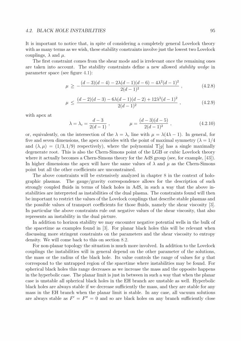
4.2. BLACK HOLE INSTABILITIES 95
It is important to notice that, in spite of considering a completely general Lovelock theorywith as many terms as we wish, these stability constraints involve just the lowest two Lovelockcouplings, λ and µ.
The first constraint comes from the shear mode and is irrelevant once the remaining onesare taken into account. The stability constraints define a new allowed stability wedge inparameter space (see figure 4.1):
µ ≥ −(d− 3)(d− 4)− 2λ(d− 1)(d− 6)− 4λ2(d− 1)2
2(d− 1)2, (4.2.8)
µ ≤ (d− 2)(d− 3)− 6λ(d− 1)(d− 2) + 12λ2(d− 1)2
2(d− 1)2, (4.2.9)
with apex at
λ = λc =d− 3
2(d− 1), µ =
(d− 3)(d− 5)
2(d− 1)2, (4.2.10)
or, equivalently, on the intersection of the λ = λc line with µ = λ(4λ − 1). In general, forfive and seven dimensions, the apex coincides with the point of maximal symmetry (λ = 1/4and (λ, µ) = (1/3, 1/9) respectively), where the polynomial Υ[g] has a single maximallydegenerate root. This is also the Chern-Simons point of the LGB or cubic Lovelock theorywhere it actually becomes a Chern-Simons theory for the AdS group (see, for example, [43]).In higher dimensions the apex will have the same values of λ and µ as the Chern-Simonspoint but all the other coefficients are unconstrained.
The above constraints will be extensively analyzed in chapter 8 in the context of holo-graphic plasmas. The gauge/gravity correspondence allows for the description of suchstrongly coupled fluids in terms of black holes in AdS, in such a way that the above in-stabilities are interpreted as instabilities of the dual plasma. The constraints found will thenbe important to restrict the values of the Lovelock couplings that describe stable plasmas andthe possible values of transport coefficients for those fluids, namely the shear viscosity [3].In particular the above constraints rule out negative values of the shear viscosity, that alsorepresents an instability in the dual picture.
In addition to horizon stability we may encounter negative potential wells in the bulk ofthe spacetime as examples found in [3]. For planar black holes this will be relevant whendiscussing more stringent constraints on the parameters and the shear viscosity to entropydensity. We will come back to this on section 8.2.
For non-planar topology the situation is much more involved. In addition to the Lovelockcouplings the instabilities will in general depend on the other parameter of the solutions,the mass or the radius of the black hole. Its value controls the range of values for g thatcorrespond to the untrapped region of the spacetime where instabilities may be found. Forspherical black holes this range decreases as we increase the mass and the opposite happensin the hyperbolic case. The planar limit is just in between in such a way that when the planarcase is unstable all spherical black holes in the EH branch are unstable as well. Hyperbolicblack holes are always stable if we decrease sufficiently the mass, and they are stable for anymass in the EH branch when the planar limit is stable. In any case, all vacuum solutionsare always stable as F ′ = F ′′ = 0 and so are black holes on any branch sufficiently close
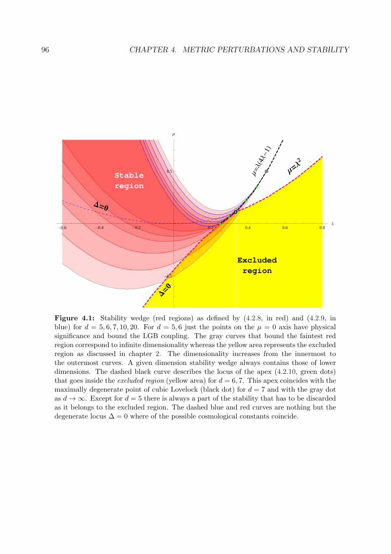
96 CHAPTER 4. METRIC PERTURBATIONS AND STABILITY
-0.6 -0.4 -0.2 0.2 0.4 0.6 0.8Λ
-0.5
0.5
Μ
Μ=Λ2
Μ=
ΛH4Λ
-1L
D=0
D=0
Excludedregion
Stableregion
Figure 4.1: Stability wedge (red regions) as defined by (4.2.8, in red) and (4.2.9, inblue) for d = 5, 6, 7, 10, 20. For d = 5, 6 just the points on the µ = 0 axis have physicalsignificance and bound the LGB coupling. The gray curves that bound the faintest redregion correspond to infinite dimensionality whereas the yellow area represents the excludedregion as discussed in chapter 2. The dimensionality increases from the innermost tothe outermost curves. A given dimension stability wedge always contains those of lowerdimensions. The dashed black curve describes the locus of the apex (4.2.10, green dots)that goes inside the excluded region (yellow area) for d = 6, 7. This apex coincides with themaximally degenerate point of cubic Lovelock (black dot) for d = 7 and with the gray dotas d→∞. Except for d = 5 there is always a part of the stability that has to be discardedas it belongs to the excluded region. The dashed blue and red curves are nothing but thedegenerate locus ∆ = 0 where of the possible cosmological constants coincide.
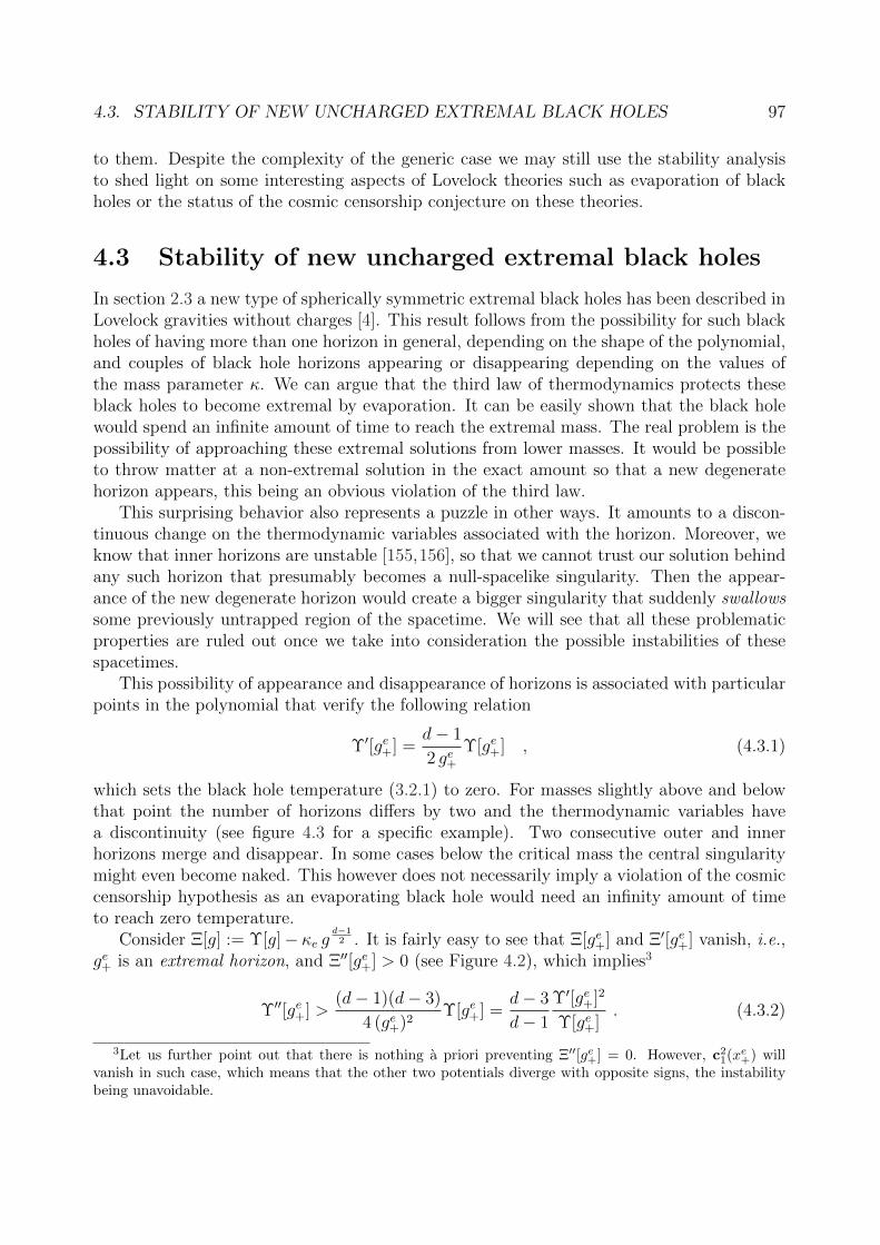
4.3. STABILITY OF NEW UNCHARGED EXTREMAL BLACK HOLES 97
to them. Despite the complexity of the generic case we may still use the stability analysisto shed light on some interesting aspects of Lovelock theories such as evaporation of blackholes or the status of the cosmic censorship conjecture on these theories.
4.3 Stability of new uncharged extremal black holes
In section 2.3 a new type of spherically symmetric extremal black holes has been described inLovelock gravities without charges [4]. This result follows from the possibility for such blackholes of having more than one horizon in general, depending on the shape of the polynomial,and couples of black hole horizons appearing or disappearing depending on the values ofthe mass parameter κ. We can argue that the third law of thermodynamics protects theseblack holes to become extremal by evaporation. It can be easily shown that the black holewould spend an infinite amount of time to reach the extremal mass. The real problem is thepossibility of approaching these extremal solutions from lower masses. It would be possibleto throw matter at a non-extremal solution in the exact amount so that a new degeneratehorizon appears, this being an obvious violation of the third law.
This surprising behavior also represents a puzzle in other ways. It amounts to a discon-tinuous change on the thermodynamic variables associated with the horizon. Moreover, weknow that inner horizons are unstable [155,156], so that we cannot trust our solution behindany such horizon that presumably becomes a null-spacelike singularity. Then the appear-ance of the new degenerate horizon would create a bigger singularity that suddenly swallowssome previously untrapped region of the spacetime. We will see that all these problematicproperties are ruled out once we take into consideration the possible instabilities of thesespacetimes.
This possibility of appearance and disappearance of horizons is associated with particularpoints in the polynomial that verify the following relation
Υ′[ge+] =d− 1
2 ge+Υ[ge+] , (4.3.1)
which sets the black hole temperature (3.2.1) to zero. For masses slightly above and belowthat point the number of horizons differs by two and the thermodynamic variables havea discontinuity (see figure 4.3 for a specific example). Two consecutive outer and innerhorizons merge and disappear. In some cases below the critical mass the central singularitymight even become naked. This however does not necessarily imply a violation of the cosmiccensorship hypothesis as an evaporating black hole would need an infinity amount of timeto reach zero temperature.
Consider Ξ[g] := Υ[g]− κe gd−1
2 . It is fairly easy to see that Ξ[ge+] and Ξ′[ge+] vanish, i.e.,ge+ is an extremal horizon, and Ξ′′[ge+] > 0 (see Figure 4.2), which implies3
Υ′′[ge+] >(d− 1)(d− 3)
4 (ge+)2Υ[ge+] =
d− 3
d− 1
Υ′[ge+]2
Υ[ge+]. (4.3.2)
3Let us further point out that there is nothing a priori preventing Ξ′′[ge+] = 0. However, c21(xe+) willvanish in such case, which means that the other two potentials diverge with opposite signs, the instabilitybeing unavoidable.
98 CHAPTER 4. METRIC PERTURBATIONS AND STABILITY
2 4 6g
10
20
30
40U@gD
¥r+
r-
rext
Κ=0.1
Κ=Κext
Figure 4.2: Cubic polynomial for L = 1, λ = −0.746 and µ = 0.56. The dashed lines
are just κ (g/σ)d−1
2 for d = 7 and the indicated values of σ and κ (in units of L). Thecrossing of these lines with the polynomial give the possible values for g at the horizonand then of r+. We observe the occurrence of two (outer and inner, respectively) horizons,r+ and r− which disappear for κ < κext leaving a naked singularity. For d = 8 we find asimilar behavior with one further inner horizon, three in total, with no naked singularityno matter the value of the mass.
Both conditions make no reference to the specific value of the mass but rather express aproperty of the polynomial for some particular value of g. Moreover, taking into accountthat we are considering positive mass solutions, Υ[ge+] > 0, we obtain the condition
F ′(xe+) =Υ′′[ge+]Υ[ge+]
Υ′[ge+]2>d− 3
d− 1. (4.3.3)
Remarkably this is exactly equivalent to the violation of one of the stability conditions
c21(xe+) < 0 . (4.3.4)
but also to having a negative coefficient for the graviton kinetic term in the black holebackground and thus to unitarity. As we reduce the mass approaching the extremal valuethe black hole becomes unstable, earlier than any jump in the black hole radius. The solutionis unstable also for any lower mass as the value of g for the extremal point ge would belongto the untrapped region in that case. The puzzle posed by these solutions is then solved, thepathological behavior being related to non-unitarity of the gravitons and instabilities of theblack hole. Before any pathological behavior is encountered an instability sets in driving thesystem somewhere else. By the same token, this also forbids the possibility of the previouslydescribed violations of the third law of thermodynamics.
In the case where several extremal points (or masses) exist the relevant one is always theone corresponding to the lowest value of ge (biggest radius) and the associate mass. Noticethat in general the instability is triggered for masses slightly above that extremal one.
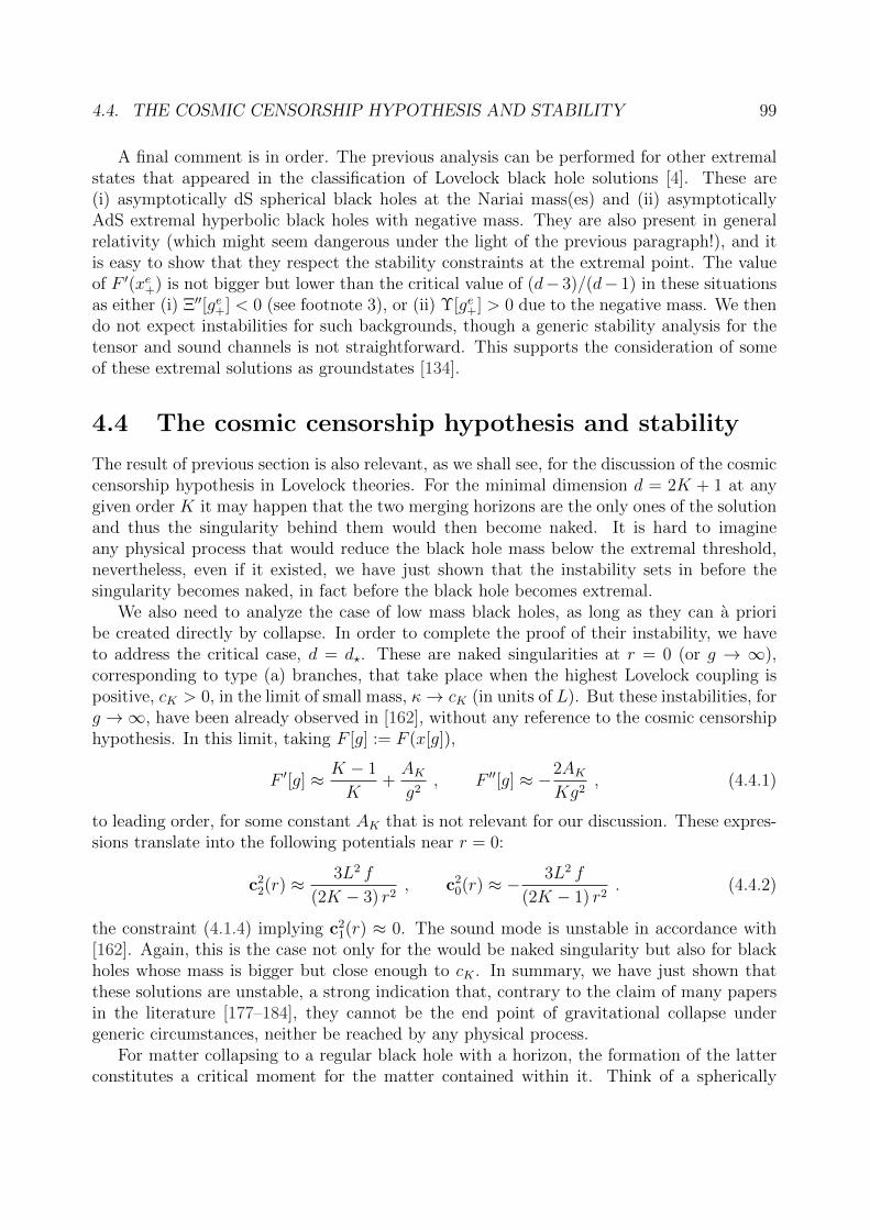
4.4. THE COSMIC CENSORSHIP HYPOTHESIS AND STABILITY 99
A final comment is in order. The previous analysis can be performed for other extremalstates that appeared in the classification of Lovelock black hole solutions [4]. These are(i) asymptotically dS spherical black holes at the Nariai mass(es) and (ii) asymptoticallyAdS extremal hyperbolic black holes with negative mass. They are also present in generalrelativity (which might seem dangerous under the light of the previous paragraph!), and itis easy to show that they respect the stability constraints at the extremal point. The valueof F ′(xe+) is not bigger but lower than the critical value of (d− 3)/(d− 1) in these situationsas either (i) Ξ′′[ge+] < 0 (see footnote 3), or (ii) Υ[ge+] > 0 due to the negative mass. We thendo not expect instabilities for such backgrounds, though a generic stability analysis for thetensor and sound channels is not straightforward. This supports the consideration of someof these extremal solutions as groundstates [134].
4.4 The cosmic censorship hypothesis and stability
The result of previous section is also relevant, as we shall see, for the discussion of the cosmiccensorship hypothesis in Lovelock theories. For the minimal dimension d = 2K + 1 at anygiven order K it may happen that the two merging horizons are the only ones of the solutionand thus the singularity behind them would then become naked. It is hard to imagineany physical process that would reduce the black hole mass below the extremal threshold,nevertheless, even if it existed, we have just shown that the instability sets in before thesingularity becomes naked, in fact before the black hole becomes extremal.
We also need to analyze the case of low mass black holes, as long as they can a prioribe created directly by collapse. In order to complete the proof of their instability, we haveto address the critical case, d = d?. These are naked singularities at r = 0 (or g → ∞),corresponding to type (a) branches, that take place when the highest Lovelock coupling ispositive, cK > 0, in the limit of small mass, κ→ cK (in units of L). But these instabilities, forg →∞, have been already observed in [162], without any reference to the cosmic censorshiphypothesis. In this limit, taking F [g] := F (x[g]),
F ′[g] ≈ K − 1
K+AKg2
, F ′′[g] ≈ −2AKKg2
, (4.4.1)
to leading order, for some constant AK that is not relevant for our discussion. These expres-sions translate into the following potentials near r = 0:
c22(r) ≈ 3L2 f
(2K − 3) r2, c2
0(r) ≈ − 3L2 f
(2K − 1) r2. (4.4.2)
the constraint (4.1.4) implying c21(r) ≈ 0. The sound mode is unstable in accordance with
[162]. Again, this is the case not only for the would be naked singularity but also for blackholes whose mass is bigger but close enough to cK . In summary, we have just shown thatthese solutions are unstable, a strong indication that, contrary to the claim of many papersin the literature [177–184], they cannot be the end point of gravitational collapse undergeneric circumstances, neither be reached by any physical process.
For matter collapsing to a regular black hole with a horizon, the formation of the latterconstitutes a critical moment for the matter contained within it. Think of a spherically
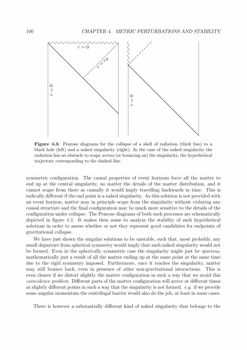
100 CHAPTER 4. METRIC PERTURBATIONS AND STABILITY
r=
0
r=rH
r = 0
r=
0
Figure 4.3: Penrose diagrams for the collapse of a shell of radiation (thick line) to ablack hole (left) and a naked singularity (right). In the case of the naked singularity theradiation has no obstacle to scape across (or bouncing on) the singularity, the hypotheticaltrajectory corresponding to the dashed line.
symmetric configuration. The causal properties of event horizons force all the matter toend up at the central singularity, no matter the details of the matter distribution, and itcannot scape from there as causally it would imply travelling backwards in time. This isradically different if the end point is a naked singularity. As this solution is not provided withan event horizon, matter may in principle scape from the singularity without violating anycausal structure and the final configuration may be much more sensitive to the details of theconfiguration under collapse. The Penrose diagrams of both such processes are schematicallydepicted in figure 4.3. It makes then sense to analyze the stability of such hypotheticalsolutions in order to assess whether or not they represent good candidates for endpoints ofgravitational collapse.
We have just shown the singular solutions to be unstable, such that, most probably, anysmall departure from spherical symmetry would imply that such naked singularity would notbe formed. Even in the spherically symmetric case the singularity might just be spurious,mathematically just a result of all the matter ending up at the same point at the same timedue to the rigid symmetry imposed. Furthermore, once it reaches the singularity, mattermay still bounce back, even in presence of other non-gravitational interactions. This iseven clearer if we distort slightly the matter configuration in such a way that we avoid thiscoincidence problem. Different parts of the matter configuration will arrive at different timesat slightly different points in such a way that the singularity is not formed. e.g. if we providesome angular momentum the centrifugal barrier would also do the job, at least in some cases.
There is however a substantially different kind of naked singularity that belongs to the
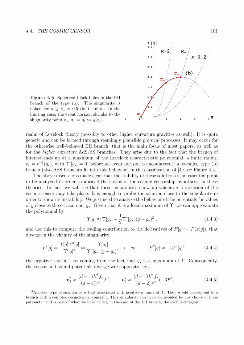
4.4. THE COSMIC CENSOR 101
Figure 4.4: Spherical black holes in the EHbranch of the type (b). The singularity isnaked for κ ≤ κ? = 0.5 (in L units). In thelimiting case, the event horizon shrinks to thesingularity point r?, g+ = g? := g(r?). -2 -1 1 2 3 4
g
0.5
1.0
1.5
2.0
2.5
3.0
3.5
U@gD
r*
¥
r+
Κ=2Κ=0.2
Κ*
HbL
realm of Lovelock theory (possibly to other higher curvature gravities as well). It is quitegeneric and can be formed through seemingly plausible physical processes. It may occur forthe otherwise well-behaved EH branch, that is the main focus of most papers, as well asfor the higher curvature AdS/dS branches. They arise due to the fact that the branch ofinterest ends up at a maximum of the Lovelock characteristic polynomial, a finite radius,r? = r−1(g?), with Υ′[g?] = 0, before an event horizon is encountered,4 a so-called type (b)branch (also AdS branches fit into this behavior) in the classification of [4]; see Figure 4.4.
The above discussions make clear that the stability of these solutions is an essential pointto be analyzed in order to unravel the status of the cosmic censorship hypothesis in thesetheories. In fact, we will see that these instabilities show up whenever a violation of thecosmic censor may take place. It is enough to probe the solution close to the singularity inorder to show its instability. We just need to analyze the behavior of the potentials for valuesof g close to the critical one, g?. Given that it is a local maximum of Υ, we can approximatethe polynomial by
Υ[g] ≈ Υ[g?] +1
2Υ′′[g?] (g − g?)2 , (4.4.3)
and use this to compute the leading contribution to the derivatives of F [g] := F (x[g]), thatdiverge in the vicinity of the singularity,
F ′[g] =Υ[g]Υ′′[g]
Υ′[g]2≈ Υ[g?]
Υ′′[g?] (g − g?)2→ −∞ , F ′′[g] ≈ −2F ′[g]2 , (4.4.4)
the negative sign in −∞ coming from the fact that g? is a maximum of Υ. Consequently,the tensor and sound potentials diverge with opposite sign,
c22 ≈
(d− 1)L2 f?(d− 4) r2
F ′ , c20 ≈
(d− 1)L2 f?(d− 2) r2
(−3F ′) . (4.4.5)
4Another type of singularity is that associated with positive minima of Υ. They would correspond to abranch with a complex cosmological constant. This singularity can never be avoided by any choice of massparameter and is part of what we have called, in the case of the EH branch, the excluded region.
102 CHAPTER 4. METRIC PERTURBATIONS AND STABILITY
this being a clear sign of unavoidable instability. Again, since we have expanded aroundr?, not only the naked singularity is unstable but any black hole solution whose horizonis close enough to it, r+ ' r?; i.e., κ & κ?. Hence, the black hole solutions cannot becontinuously connected to the singular solution by any physical process since the instabilitywould inevitably show up with increasing importance before the singularity is attained,driving the system somewhere else. This is an important point, as long as the thresholdbetween type (b) black holes and naked singularities is not an extremal solution. As thehorizon approaches the singularity, given that F ′ diverges in that limit, the instability isincreasingly important and dramatic when we get there.
4.5 Instabilities and black hole evaporation
In our quest to qualitatively understand in which situations Lovelock black holes becomeunstable we pass on to the case of evaporating black holes. This case is relevant as in pre-vious analysis the instabilities under study seem to appear whenever the black hole horizonapproaches too much the singularity. This is for instance what happens for type (b) spheri-cal solutions. As the black hole evaporates it looses mass approaching the critical value (forwhich the temperature diverges) in finite time. This would leave behind a naked singularitybut we already proved that neither the extremal solution nor the naked singularity can bereached, the solution becomes unstable as the horizon gets close to the singularity.
The same happens for the other cases analyzed throughout this chapter and the samewill also hold for other classes of evaporating spherical black holes. We have also seen thatfor type (a) branches in d = 2K + 1 the black hole solution becomes unstable as well beforereaching the r+ = 0 state, that in this case is extremal. The black hole would spend aninfinite amount of time to become extremal but just a finite amount to reach the instability.Hence, the instability seem to play a role in the evaporation process of black holes in Lovelockgravities, at least for spherical topology.
The remaining case to be understood is that of type (a) solutions, either on the EH ordS branches, for dimensions bigger than the critical, d > 2K + 1. As the mass of the blackhole shrinks to zero the horizon also shrinks approaching the central singularity. In thiscase the singularity can never become naked but still instabilities show up before the blackhole shrinks to zero size. In [162, 191] it has been observed that when all possible Lovelockcouplings are turned on – the highest one being positive, cK > 0 – the instability alwaysshows up, in even and odd dimensions. Here we will generalize that analysis.
Expanding the tensor and scalar potentials around g →∞ we simply get
c22 ≈
(d− 3K − 1)L2 f
K(d− 4) r2, c2
0 ≈(d−K − 1)L2 f
K(d− 2) r2. (4.5.1)
Then any spherical branch under the above conditions will present a tensor instability in thesmall mass limit for 2K + 1 < d < 3K + 1, where K is the order of the Lovelock theory.Einstein-Hilbert is a special case from this perspective. The d = 3K + 1 is special and weneed to go to the following order in the tensor potential. In that case whether the black holeis stable or not will depend on the actual values of (cK−1/cK)2 and cK−2/cK . The case ofEinstein-Hilbert gravity is stable in any number of dimensions.
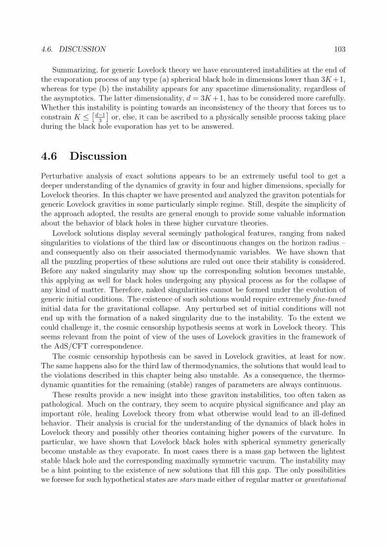
4.6. DISCUSSION 103
Summarizing, for generic Lovelock theory we have encountered instabilities at the end ofthe evaporation process of any type (a) spherical black hole in dimensions lower than 3K+1,whereas for type (b) the instability appears for any spacetime dimensionality, regardless ofthe asymptotics. The latter dimensionality, d = 3K+1, has to be considered more carefully.Whether this instability is pointing towards an inconsistency of the theory that forces us toconstrain K ≤
[d−1
3
]or, else, it can be ascribed to a physically sensible process taking place
during the black hole evaporation has yet to be answered.
4.6 Discussion
Perturbative analysis of exact solutions appears to be an extremely useful tool to get adeeper understanding of the dynamics of gravity in four and higher dimensions, specially forLovelock theories. In this chapter we have presented and analyzed the graviton potentials forgeneric Lovelock gravities in some particularly simple regime. Still, despite the simplicity ofthe approach adopted, the results are general enough to provide some valuable informationabout the behavior of black holes in these higher curvature theories.
Lovelock solutions display several seemingly pathological features, ranging from nakedsingularities to violations of the third law or discontinuous changes on the horizon radius –and consequently also on their associated thermodynamic variables. We have shown thatall the puzzling properties of these solutions are ruled out once their stability is considered.Before any naked singularity may show up the corresponding solution becomes unstable,this applying as well for black holes undergoing any physical process as for the collapse ofany kind of matter. Therefore, naked singularities cannot be formed under the evolution ofgeneric initial conditions. The existence of such solutions would require extremely fine-tunedinitial data for the gravitational collapse. Any perturbed set of initial conditions will notend up with the formation of a naked singularity due to the instability. To the extent wecould challenge it, the cosmic censorship hypothesis seems at work in Lovelock theory. Thisseems relevant from the point of view of the uses of Lovelock gravities in the framework ofthe AdS/CFT correspondence.
The cosmic censorship hypothesis can be saved in Lovelock gravities, at least for now.The same happens also for the third law of thermodynamics, the solutions that would lead tothe violations described in this chapter being also unstable. As a consequence, the thermo-dynamic quantities for the remaining (stable) ranges of parameters are always continuous.
These results provide a new insight into these graviton instabilities, too often taken aspathological. Much on the contrary, they seem to acquire physical significance and play animportant role, healing Lovelock theory from what otherwise would lead to an ill-definedbehavior. Their analysis is crucial for the understanding of the dynamics of black holes inLovelock theory and possibly other theories containing higher powers of the curvature. Inparticular, we have shown that Lovelock black holes with spherical symmetry genericallybecome unstable as they evaporate. In most cases there is a mass gap between the lighteststable black hole and the corresponding maximally symmetric vacuum. The instability maybe a hint pointing to the existence of new solutions that fill this gap. The only possibilitieswe foresee for such hypothetical states are stars made either of regular matter or gravitational
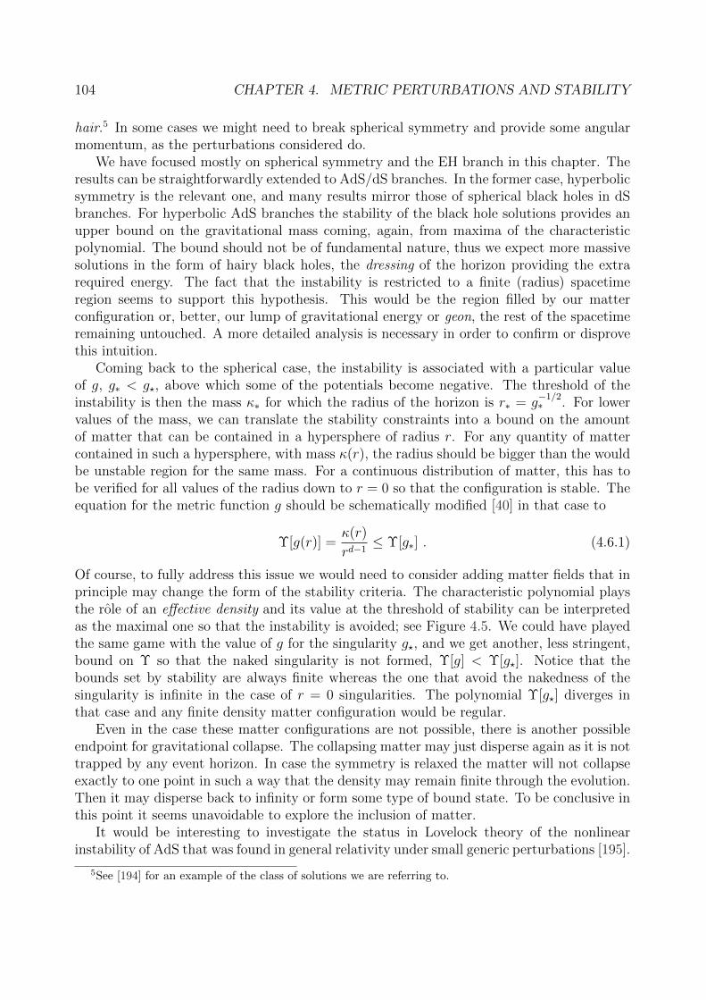
104 CHAPTER 4. METRIC PERTURBATIONS AND STABILITY
hair.5 In some cases we might need to break spherical symmetry and provide some angularmomentum, as the perturbations considered do.
We have focused mostly on spherical symmetry and the EH branch in this chapter. Theresults can be straightforwardly extended to AdS/dS branches. In the former case, hyperbolicsymmetry is the relevant one, and many results mirror those of spherical black holes in dSbranches. For hyperbolic AdS branches the stability of the black hole solutions provides anupper bound on the gravitational mass coming, again, from maxima of the characteristicpolynomial. The bound should not be of fundamental nature, thus we expect more massivesolutions in the form of hairy black holes, the dressing of the horizon providing the extrarequired energy. The fact that the instability is restricted to a finite (radius) spacetimeregion seems to support this hypothesis. This would be the region filled by our matterconfiguration or, better, our lump of gravitational energy or geon, the rest of the spacetimeremaining untouched. A more detailed analysis is necessary in order to confirm or disprovethis intuition.
Coming back to the spherical case, the instability is associated with a particular valueof g, g∗ < g?, above which some of the potentials become negative. The threshold of theinstability is then the mass κ∗ for which the radius of the horizon is r∗ = g
−1/2∗ . For lower
values of the mass, we can translate the stability constraints into a bound on the amountof matter that can be contained in a hypersphere of radius r. For any quantity of mattercontained in such a hypersphere, with mass κ(r), the radius should be bigger than the wouldbe unstable region for the same mass. For a continuous distribution of matter, this has tobe verified for all values of the radius down to r = 0 so that the configuration is stable. Theequation for the metric function g should be schematically modified [40] in that case to
Υ[g(r)] =κ(r)
rd−1≤ Υ[g∗] . (4.6.1)
Of course, to fully address this issue we would need to consider adding matter fields that inprinciple may change the form of the stability criteria. The characteristic polynomial playsthe role of an effective density and its value at the threshold of stability can be interpretedas the maximal one so that the instability is avoided; see Figure 4.5. We could have playedthe same game with the value of g for the singularity g?, and we get another, less stringent,bound on Υ so that the naked singularity is not formed, Υ[g] < Υ[g?]. Notice that thebounds set by stability are always finite whereas the one that avoid the nakedness of thesingularity is infinite in the case of r = 0 singularities. The polynomial Υ[g?] diverges inthat case and any finite density matter configuration would be regular.
Even in the case these matter configurations are not possible, there is another possibleendpoint for gravitational collapse. The collapsing matter may just disperse again as it is nottrapped by any event horizon. In case the symmetry is relaxed the matter will not collapseexactly to one point in such a way that the density may remain finite through the evolution.Then it may disperse back to infinity or form some type of bound state. To be conclusive inthis point it seems unavoidable to explore the inclusion of matter.
It would be interesting to investigate the status in Lovelock theory of the nonlinearinstability of AdS that was found in general relativity under small generic perturbations [195].
5See [194] for an example of the class of solutions we are referring to.
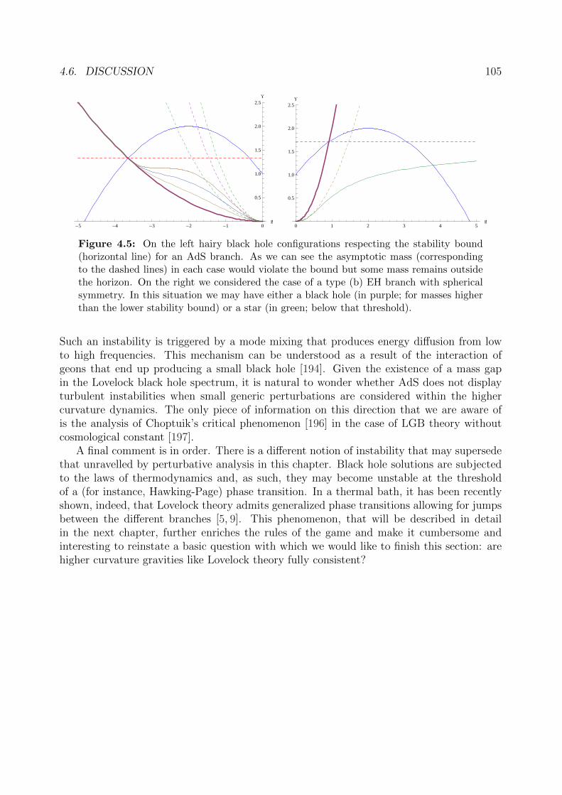
4.6. DISCUSSION 105
-5 -4 -3 -2 -1 0g
0.5
1.0
1.5
2.0
2.5U
0 1 2 3 4 5g
0.5
1.0
1.5
2.0
2.5U
Figure 4.5: On the left hairy black hole configurations respecting the stability bound(horizontal line) for an AdS branch. As we can see the asymptotic mass (correspondingto the dashed lines) in each case would violate the bound but some mass remains outsidethe horizon. On the right we considered the case of a type (b) EH branch with sphericalsymmetry. In this situation we may have either a black hole (in purple; for masses higherthan the lower stability bound) or a star (in green; below that threshold).
Such an instability is triggered by a mode mixing that produces energy diffusion from lowto high frequencies. This mechanism can be understood as a result of the interaction ofgeons that end up producing a small black hole [194]. Given the existence of a mass gapin the Lovelock black hole spectrum, it is natural to wonder whether AdS does not displayturbulent instabilities when small generic perturbations are considered within the highercurvature dynamics. The only piece of information on this direction that we are aware ofis the analysis of Choptuik’s critical phenomenon [196] in the case of LGB theory withoutcosmological constant [197].
A final comment is in order. There is a different notion of instability that may supersedethat unravelled by perturbative analysis in this chapter. Black hole solutions are subjectedto the laws of thermodynamics and, as such, they may become unstable at the thresholdof a (for instance, Hawking-Page) phase transition. In a thermal bath, it has been recentlyshown, indeed, that Lovelock theory admits generalized phase transitions allowing for jumpsbetween the different branches [5, 9]. This phenomenon, that will be described in detailin the next chapter, further enriches the rules of the game and make it cumbersome andinteresting to reinstate a basic question with which we would like to finish this section: arehigher curvature gravities like Lovelock theory fully consistent?

106 CHAPTER 4. METRIC PERTURBATIONS AND STABILITY
Chapter 5
Bubbles and new phase transitions
“Nothing has such power to broaden the mindas the ability to investigate systematically and truly
all that comes under thy observation in life.”
Marcus Aurelius
Phase transitions between two competing vacua of a given theory are a quite common phe-nomenon in physics. They occur when some parameter of the system is varied so that the(free) energy of the initial vacuum becomes greater than the other. If the energy barrierbetween the two is big enough, the system may stay in the false vacuum for some time(metastability), and proceed to decay via quantum tunneling or, at finite temperature, jumpover the wall due to a thermal kick. The decay of metastable systems usually proceedsby nucleation of bubbles of true vacuum inside the false vacuum. In field theories at zerotemperature, this was first studied by Coleman in his classic paper [198]. There, he in-troduced Euclidean methods for computing the probability of the quantum nucleation of abubble, whose dynamics, after nucleation, may be followed classically. In the first (tree-level)semiclassical approximation, the probability of bubble nucleation is given by
P ∝ e−I , (5.0.1)
where I is the Euclidean action of the system evaluated at the appropriate solution; in thiscase, the instanton. It is a time-dependent solution which, in the simplest case of a particle ina potential, starts and ends its trajectory at the bottom of the false vacuum (given that thepotential in the Euclidean section is the negative of its Lorentzian counterpart, it is a localmaximum). This is the point x = xF in figure 5.1(b), where the particle starts its trajectory,then bounces at x = xB, and finally gets back to xF in infinite time. The work of Coleman
107
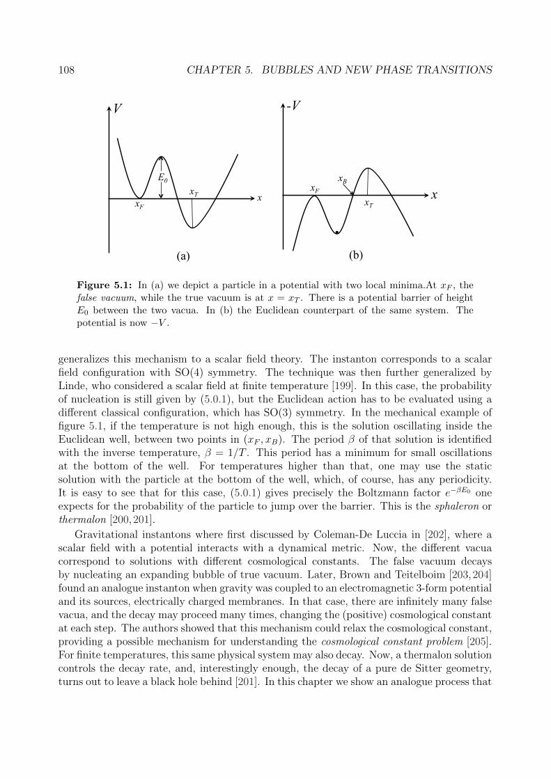
108 CHAPTER 5. BUBBLES AND NEW PHASE TRANSITIONS
V
x xF
xT
E0
-V
x xF
xT
xB
(a) (b)
Figure 5.1: In (a) we depict a particle in a potential with two local minima.At xF , thefalse vacuum, while the true vacuum is at x = xT . There is a potential barrier of heightE0 between the two vacua. In (b) the Euclidean counterpart of the same system. Thepotential is now −V .
generalizes this mechanism to a scalar field theory. The instanton corresponds to a scalarfield configuration with SO(4) symmetry. The technique was then further generalized byLinde, who considered a scalar field at finite temperature [199]. In this case, the probabilityof nucleation is still given by (5.0.1), but the Euclidean action has to be evaluated using adifferent classical configuration, which has SO(3) symmetry. In the mechanical example offigure 5.1, if the temperature is not high enough, this is the solution oscillating inside theEuclidean well, between two points in (xF , xB). The period β of that solution is identifiedwith the inverse temperature, β = 1/T . This period has a minimum for small oscillationsat the bottom of the well. For temperatures higher than that, one may use the staticsolution with the particle at the bottom of the well, which, of course, has any periodicity.It is easy to see that for this case, (5.0.1) gives precisely the Boltzmann factor e−βE0 oneexpects for the probability of the particle to jump over the barrier. This is the sphaleron orthermalon [200,201].
Gravitational instantons where first discussed by Coleman-De Luccia in [202], where ascalar field with a potential interacts with a dynamical metric. Now, the different vacuacorrespond to solutions with different cosmological constants. The false vacuum decaysby nucleating an expanding bubble of true vacuum. Later, Brown and Teitelboim [203,204]found an analogue instanton when gravity was coupled to an electromagnetic 3-form potentialand its sources, electrically charged membranes. In that case, there are infinitely many falsevacua, and the decay may proceed many times, changing the (positive) cosmological constantat each step. The authors showed that this mechanism could relax the cosmological constant,providing a possible mechanism for understanding the cosmological constant problem [205].For finite temperatures, this same physical system may also decay. Now, a thermalon solutioncontrols the decay rate, and, interestingly enough, the decay of a pure de Sitter geometry,turns out to leave a black hole behind [201]. In this chapter we show an analogue process that
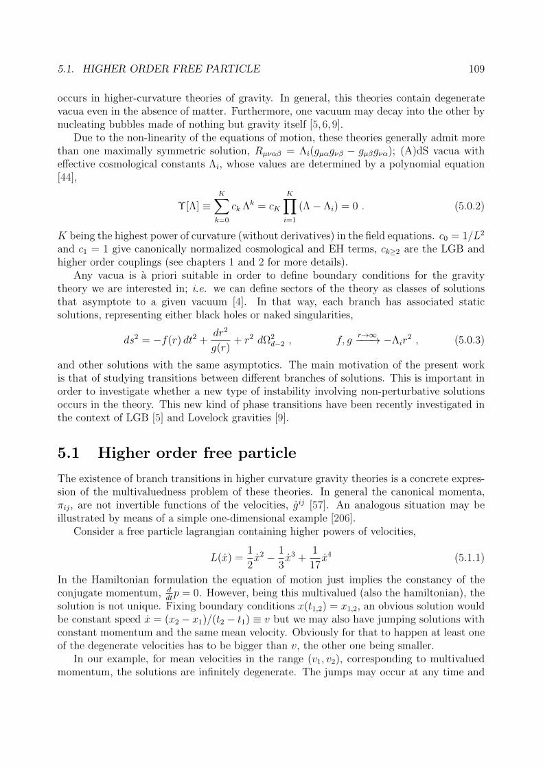
5.1. HIGHER ORDER FREE PARTICLE 109
occurs in higher-curvature theories of gravity. In general, this theories contain degeneratevacua even in the absence of matter. Furthermore, one vacuum may decay into the other bynucleating bubbles made of nothing but gravity itself [5, 6, 9].
Due to the non-linearity of the equations of motion, these theories generally admit morethan one maximally symmetric solution, Rµναβ = Λi(gµαgνβ − gµβgνα); (A)dS vacua witheffective cosmological constants Λi, whose values are determined by a polynomial equation[44],
Υ[Λ] ≡K∑k=0
ck Λk = cK
K∏i=1
(Λ− Λi) = 0 . (5.0.2)
K being the highest power of curvature (without derivatives) in the field equations. c0 = 1/L2
and c1 = 1 give canonically normalized cosmological and EH terms, ck≥2 are the LGB andhigher order couplings (see chapters 1 and 2 for more details).
Any vacua is a priori suitable in order to define boundary conditions for the gravitytheory we are interested in; i.e. we can define sectors of the theory as classes of solutionsthat asymptote to a given vacuum [4]. In that way, each branch has associated staticsolutions, representing either black holes or naked singularities,
ds2 = −f(r) dt2 +dr2
g(r)+ r2 dΩ2
d−2 , f, gr→∞−−−→ −Λir
2 , (5.0.3)
and other solutions with the same asymptotics. The main motivation of the present workis that of studying transitions between different branches of solutions. This is important inorder to investigate whether a new type of instability involving non-perturbative solutionsoccurs in the theory. This new kind of phase transitions have been recently investigated inthe context of LGB [5] and Lovelock gravities [9].
5.1 Higher order free particle
The existence of branch transitions in higher curvature gravity theories is a concrete expres-sion of the multivaluedness problem of these theories. In general the canonical momenta,πij, are not invertible functions of the velocities, gij [57]. An analogous situation may beillustrated by means of a simple one-dimensional example [206].
Consider a free particle lagrangian containing higher powers of velocities,
L(x) =1
2x2 − 1
3x3 +
1
17x4 (5.1.1)
In the Hamiltonian formulation the equation of motion just implies the constancy of theconjugate momentum, d
dtp = 0. However, being this multivalued (also the hamiltonian), the
solution is not unique. Fixing boundary conditions x(t1,2) = x1,2, an obvious solution wouldbe constant speed x = (x2 − x1)/(t2 − t1) ≡ v but we may also have jumping solutions withconstant momentum and the same mean velocity. Obviously for that to happen at least oneof the degenerate velocities has to be bigger than v, the other one being smaller.
In our example, for mean velocities in the range (v1, v2), corresponding to multivaluedmomentum, the solutions are infinitely degenerate. The jumps may occur at any time and
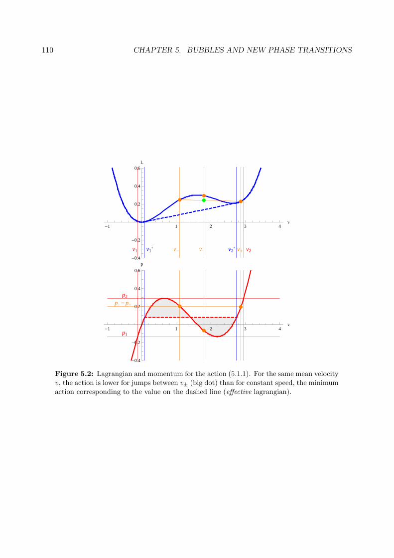
110 CHAPTER 5. BUBBLES AND NEW PHASE TRANSITIONS
-1 1 2 3 4v
-0.4
-0.2
0.2
0.4
0.6L
v1 v2v1 ' v2 'v- v v+
-1 1 2 3 4v
-0.4
-0.2
0.2
0.4
0.6
p
p2
p1
p-=p+
Figure 5.2: Lagrangian and momentum for the action (5.1.1). For the same mean velocityv, the action is lower for jumps between v± (big dot) than for constant speed, the minimumaction corresponding to the value on the dashed line (effective lagrangian).
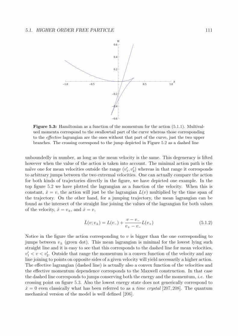
5.1. HIGHER ORDER FREE PARTICLE 111
-1.0 -0.5 0.5 1.0p
-0.6
-0.4
-0.2
0.2
0.4
0.6H
Figure 5.3: Hamiltonian as a function of the momentum for the action (5.1.1). Multival-ued momenta correspond to the swallowtail part of the curve whereas those correspondingto the effective lagrangian are the ones without that part of the curve, just the two upperbranches. The crossing correspond to the jump depicted in Figure 5.2 as a dashed line
unboundedly in number, as long as the mean velocity is the same. This degeneracy is liftedhowever when the value of the action is taken into account. The minimal action path is thenaıve one for mean velocities outside the range (v′1, v
′2) whereas in that range it corresponds
to arbitrary jumps between the two extremal velocities. One can actually compare the actionfor both kinds of trajectories directly in the figure, we have depicted one example. In thetop figure 5.2 we have plotted the lagrangian as a function of the velocity. When this isconstant, x = v, the action will just be the lagrangian L(v) multiplied by the time span ofthe trajectory. On the other hand, for a jumping trajectory, the mean lagrangian can befound as the intersect of the straight line joining the values of the lagrangian for both valuesof the velocity, x = v±, and x = v,
L(v; v±) = L(v−) +v − v−v+ − v−
L(v+) (5.1.2)
Notice in the figure the action corresponding to v is bigger than the one corresponding tojumps between v± (green dot). This mean lagrangian is minimal for the lowest lying suchstraight line and it is easy to see that this corresponds to the dashed line for mean velocities,v′1 < v < v′2. Outside that range the momentum is a convex function of the velocity and anyline joining to points on opposite sides of a given velocity will yield necessarily a higher action.The effective lagrangian (dashed line) is actually also a convex function of the velocities andthe effective momentum dependence corresponds to the Maxwell construction. In that casethe dashed line corresponds to jumps conserving both the energy and the momentum, i.e. thecrossing point on figure 5.3. Also the lowest energy state does not generically correspond tox = 0 even classically what has been referred to as a time crystal [207, 208]. The quantummechanical version of the model is well defined [206].
112 CHAPTER 5. BUBBLES AND NEW PHASE TRANSITIONS
In the presence of a potential, the naıve choice of continuous velocities runs into problemsas we would hit the degenerate points d
dxp = 0 where the acceleration is not well defined.
In the above effective approach however the momentum is a monotonous function of thevelocity except at the transition that correspond to conservation of not only momentum butenergy.
5.2 Generalized Hawking-Page transitions
In the context of general relativity in asymptotically AdS spacetimes, the Hawking-Pagephase transition [126] is the realization that above certain temperature the dominant saddlein the gravitational partition function comes from a black hole, whereas for lower temper-atures it corresponds to the thermal vacuum. The classical solution is the one with leastEuclidean action among those with a smooth Euclidean section. In the case of Lovelockgravities the occurrence of these transitions was analyzed in chapter 3.
When one deals with higher curvature gravity however there is a crucial difference thathas been overlooked in the literature. In addition to the usual continuous and differentiablemetrics (5.0.3), one may construct distributional metrics by gluing two solutions correspond-ing to different branches across a spherical shell or bubble [55, 56]. The resulting solutionwill be continuous at the bubble –with discontinuous derivatives, even in absence of matter.The higher curvature terms can be thought of as a sort of matter source for the Einsteintensor. The existence of such jump metrics, as for the one-dimensional example, is due tothe multivaluedness of momenta in the theory.
In the gravitational context, continuity of momenta is equivalent to the junction condi-tions that need to be imposed on the bubble. In the EH case, Israel junction conditions [49],being linear in velocities, also imply the continuity of derivatives of the metric. The gener-alization of these conditions for higher curvature gravity contain higher powers of velocities,thus allowing for more general situations.
Static bubble configurations, when they exist, have a smooth Euclidean continuation. Itis then possible to calculate the value of the action and compare it to all other solutionswith the same asymptotics and temperature. This analysis has been performed for the LGBaction [5] for unstable boundary conditions [44]. The result suggests a possible resolution ofthe instability through bubble nucleation.
The phenomenon described here is quite general. It occurs also for general Lovelockgravities [9] and presumably for more general classes of theories. One may even think of thepossibility of having different gravity theories on different sides of the bubble. This has astraightforward physical interpretation if we consider the higher order terms as sourced byother fields that vary across the bubble. For masses above m2 > ‖Λ±‖ a bubble made ofthese fields will be well approximated by a thin wall and we may integrate out the fields forthe purpose of discussing the thermodynamics. If those fields have several possible vacuumexpectation values leading to different theories we may construct interpolating solutions inessentially the same way discussed in this chapter. In this case the energy carried by thebubble can be interpreted as the energy of the fields we have integrated out.
5.3. JUNCTION CONDITIONS 113
5.3 Junction conditions
We are interested in configurations involving a (timelike, n2 = 1) junction surface dividingtwo regions, each of them given by a solution corresponding to a different branch of theLovelock action. To this end, we will split the geometry asM =M− ∪ (Σ×ξ) ∪M+, whereM∓ denote the interior/exterior regions respectively, Σ is the codimension one junction(hyper)surface, and ξ ∈ [0, 1] is a real parameter used to interpolate both regions. Thematching condition can be obtained from an action principle constructed by means of twoauxiliary quantities [209]
Ea = ξ ea+ + (1− ξ) ea− , Ωab = ξ ωab+ + (1− ξ)ωab− , (5.3.1)
and the associated generalized curvatures
Rabξ = dΩab + Ωa
c ∧Ωcb = ξ Rab+ + (1− ξ)Rab
− − ξ(1− ξ) (ω+ − ω−)ac ∧ (ω+ − ω−)cb , (5.3.2)
and Fab = δΩab +Rab, where δ is the exterior derivative on the convex simplex in the spaceof connections, δ = dξ ∂
∂ξ. That is, δΩab = dξ ∧ (ωab+ − ωab− ). These curvatures are used
to construct the secondary characteristic classes [210]. Their use in the context of Chern–Simons gravities has been considered in [211].
In the bulk regions ξ takes a fixed value, ξ = 0, 1 respectively in M∓, whereas it runsfrom 0 to 1 in Σ and has to be integrated over. The so-called secondary action is obtainedby substituting ea by Ea and Rab by Fab in (1.1.1),
Lk = εa1a2···adFa1a2 ∧ · · · ∧ Fa2k−1a2k ∧ Ea2k+1···ad , (5.3.3)
We can readily expand the secondary action in powers of δΩ, taking into account thatδΩ∧ δΩ = 0. The leading term corresponds to the bulk integrals onM∓ and contributes tothe standard Lovelock action (1.1.1), while the first order term captures the integral alongξ on Σ,
Qk = −k∫ 1
0
dξ (ω+ − ω−)a1a2 ∧Ra3a4 ∧ · · · ∧ Ra2k−1a2k ∧ Ea2k+1···adεa1···ad , (5.3.4)
where the minus sign has been chosen so that it coincides with the sign in section 1.2. If wefurther impose the continuity of the metric such that Ea = ea for some choice of vielbein,we may also define θab± = ωab± − ωab0 . From this ωab+ − ωab− can be replaced by θab+ − θab− , whichis zero unless one of the indices lies along the normal direction. Thus, the only relevantcontributions to Rab are those whose two indices are tangent to Σ. Now,
Rab = Rab0 + Θa
c ∧Θcb + . . . , (5.3.5)
where Rab0 is the intrinsic curvature of Σ computed from ωab0 , Θab ≡ ξ θab+ + (1 − ξ) θab− , and
the dots amount to terms having at least one index in the normal direction. Recalling therelation between the second fundamental form and the extrinsic curvature (1.2.30), we canfinally write
Qk = 2k
∫ 1
0
dξ(K+ −K−)A1 ∧RA2A3j ∧ · · · ∧R
A2k−2A2k−1
j ∧ eA2k···AdεA1···Ad , (5.3.6)
114 CHAPTER 5. BUBBLES AND NEW PHASE TRANSITIONS
where the junction generalized curvature RABj (ξ), is given by RAB
j (ξ) ≡ RAB0 − (ξ KA
+ + (1−ξ)KA
−) ∧ (ξ KB+ + (1 − ξ)KB
− ) (we can recover the boundary generalized curvature (1.2.33)
by switching-off Ka+ → 0). We can surprisingly split Qk = Q−k −Q
+k , where
Q±k = −2k
∫ 1
0
dξ KA1± ∧RA2A3
0± (ξ) ∧ · · · ∧RA2k−2A2k−1
0± (ξ) ∧ eA2k···AdεA1···Ad , (5.3.7)
with RAB0± (ξ) ≡ RAB
0 − ξ2KA± ∧KB
± , either term coming from each boundary region. That is,the junction acts as a two-sided boundary. All in all, the kth contribution to the total actioncan be written in terms of quantities coming from both sides,
Ik =
(∫M−L−k −
∫Σ
Q−k)
+
(∫M+
L+k +
∫Σ
Q+k −
∫∂MQ+k
), (5.3.8)
the relative plus sign in the second term coming from the reverse orientation of the surfacein that region. The last term is irrelevant for the purposes of the present letter and will notbe considered in the following, it just makes the whole outer contribution to vanish if wetake the junction surface to infinity. The infinitesimal variation of the boundary action withrespect to ω± gives two terms. One is a total derivative. The other cancels with the totalderivative term coming from the bulk. The surface contribution to the equations of motionis just given by the variation with respect to the frame, that correspond on each side to thecanonical momentum at the surface. As explained in section 1.2, the junction conditionsamount just to continuity of the momenta across the hypersurface Σ defined in (1.2.39),
π+AB = π−AB . (5.3.9)
In the particular case we are interested in, given that all the forms involved in the aboveexpression are diagonal, we should only care on those components.
5.3.1 Thermalon configuration
Let us be more detailed in the kind of configurations we are interested in. They correspond toa bubble, whose outer region asymptotes AdS with a cosmological constant Λ+, while the innerregion corresponds to another branch solution characterized by the effective cosmologicalconstant Λ− (see figure 5.4). The junction conditions will constrain the possible combinationsof parameters that will describe the solutions of interest, instantons and thermalons. Acrossthe junction, the vielbein has to be continuous. We thus consider an Euclidean section ofthe form
ds2 = f±(r)dt2 +dr2
f±(r)+ r2 dΩ2
σ,d−2 , (5.3.10)
where the ± signs denote the outer/inner regions. The junction is conveniently described bythe parametric equations
r = a(τ) , t± = T±(τ) , (5.3.11)
with an induced metric of the form
ds2 = dτ 2 + a(τ)2 dΣ2d−2,σ , (5.3.12)
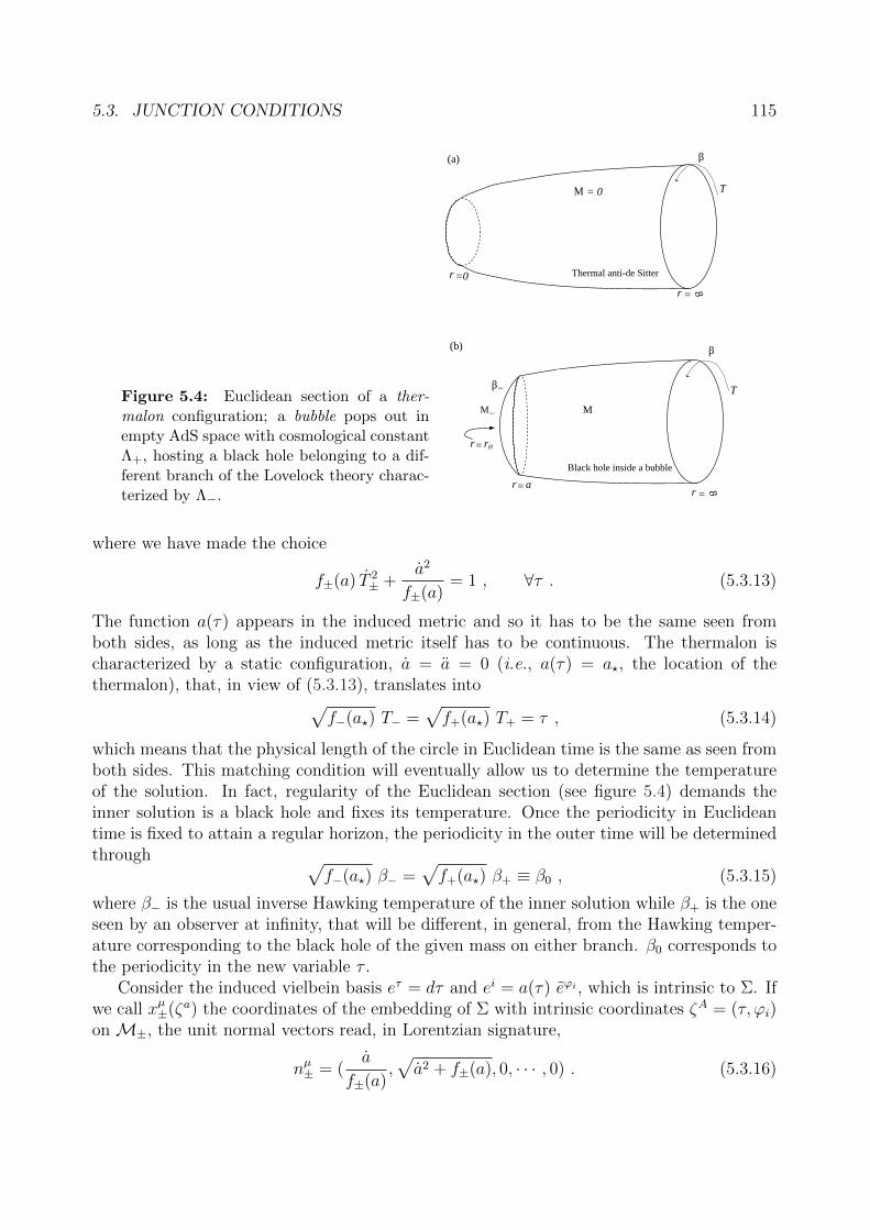
5.3. JUNCTION CONDITIONS 115
Figure 5.4: Euclidean section of a ther-malon configuration; a bubble pops out inempty AdS space with cosmological constantΛ+, hosting a black hole belonging to a dif-ferent branch of the Lovelock theory charac-terized by Λ−.
(a)
r =0
β+
r = 8T+Μ+ = 0
(b) β+
T+
r = 8r= a
r= rH
β−
Μ− Μ+
Thermal anti-de Sitter
Black hole inside a bubble
where we have made the choice
f±(a) T 2± +
a2
f±(a)= 1 , ∀τ . (5.3.13)
The function a(τ) appears in the induced metric and so it has to be the same seen fromboth sides, as long as the induced metric itself has to be continuous. The thermalon ischaracterized by a static configuration, a = a = 0 (i.e., a(τ) = a?, the location of thethermalon), that, in view of (5.3.13), translates into√
f−(a?) T− =√f+(a?) T+ = τ , (5.3.14)
which means that the physical length of the circle in Euclidean time is the same as seen fromboth sides. This matching condition will eventually allow us to determine the temperatureof the solution. In fact, regularity of the Euclidean section (see figure 5.4) demands theinner solution is a black hole and fixes its temperature. Once the periodicity in Euclideantime is fixed to attain a regular horizon, the periodicity in the outer time will be determinedthrough √
f−(a?) β− =√f+(a?) β+ ≡ β0 , (5.3.15)
where β− is the usual inverse Hawking temperature of the inner solution while β+ is the oneseen by an observer at infinity, that will be different, in general, from the Hawking temper-ature corresponding to the black hole of the given mass on either branch. β0 corresponds tothe periodicity in the new variable τ .
Consider the induced vielbein basis eτ = dτ and ei = a(τ) eϕi , which is intrinsic to Σ. Ifwe call xµ±(ζa) the coordinates of the embedding of Σ with intrinsic coordinates ζA = (τ, ϕi)on M±, the unit normal vectors read, in Lorentzian signature,
nµ± = (a
f±(a),√a2 + f±(a), 0, · · · , 0) . (5.3.16)
116 CHAPTER 5. BUBBLES AND NEW PHASE TRANSITIONS
The extrinsic curvature is then given by
KAB = −n±µ
(∂2xµ±∂ζA∂ζB
+ Γµαβ∂xα±∂ζA
∂xβ±∂ζB
), (5.3.17)
yielding
K±ττ =
a+ 12f ′±(a)√
a2 + f±(a), K±
ϕiϕj
=
√a2 + f±(a)
aδij . (5.3.18)
The intrinsic curvature, in turn, is given by
Riτ0 =
a
aei ∧ eτ , Rij
0 =σ + a2
a2ei ∧ ej . (5.3.19)
Notice that it is trivially the same as seen from either side as it is calculated from the inducedmetric and this is continuous. The vielbein basis is continuous but the spin connection isnot. In that case it should be possible to write the surface term as the difference of (1.2.33)seen from each of the bulk regions. It is clear that all the components aligned along thenormal direction of this intrinsic spin connection are zero in the same way as it happens forthe corresponding intrinsic curvature. In the Euclidean signature we may just change thesigns of the squared velocity and its acceleration as (a2, a) → (−a2
E,−aE).
5.3.2 Junction conditions and bubble dynamics
The junction conditions (5.3.9) for the configurations of interest have just diagonal compo-nents related by a conservation equation (Bianchi identity) that constrains them in such away that only the ττ component matters. The rest are related to that one as [54,55]
d
dτ
(ad−2 π±ττ
)= (d− 2) a2a π±ϕiϕi , ∀i , (5.3.20)
in such a way that if π±ττ verifies (5.3.9), all the components automatically do. This isreminiscent of the analogous field equations for cosmological solutions studied in section2.6 Thus, we just need to compute π±ττ . This junction condition involves just the angularcomponents of both the intrinsic and extrinsic curvatures; the expression reduces to
Π±(ττ) ≡√a2 + f±(a)
a
∫ 1
0
dξ Υ′[σ − ξ2 f±(a) + (1− ξ2) a2
a2
], (5.3.21)
where we avoid the inclusion of some (irrelevant for our discussion) factors, and the poly-nomial Υ is again seen to play a central role. In the future we will also avoid the use ofindices, Π± referring to the (ττ)-component. If we define Π = Π+ −Π−, because of (5.3.20)
the junction equations can be written as Π = ∂τ Π = 0. Notice that the dimensionalityof spacetime is somehow irrelevant in this expression. In the case of LGB, this expressionreduces to the one in [56]. If we conveniently introduce the functions1
g± ≡ g±(a) =σ − f±(a)
a2, H ≡ H(a, a) =
σ + a2
a2, (5.3.22)
1Not to be confused with the previously used notation for the horizon value of g, 1/r2+
5.3. JUNCTION CONDITIONS 117
we can rewrite
Π± [g±, H] =√H − g±
∫ 1
0
dξ Υ′[ξ2 g± + (1− ξ2)H
], (5.3.23)
where it becomes clear that all the information about the branches is contained in g±, thatare implicitly given by (2.1.8). Notice that g± ≤ H in order to have a real value for Π±
(which tantamount to f±(a) ≥ 0 in order to have a real Euclidean boundary action). Thisimplies that the static bubble corresponding to the thermalon necessarily forms at a? ≥max(rH+, rH−), outside the would be black hole horizons corresponding to both branches.Moreover, this reality condition is also necessary for the equation to yield real values of thevelocity, at least for some region of the spacetime.
The difference in canonical momenta Π may be rewritten in a couple more useful waysas
Π =
∫ 1
0
dξ(√
H − g+ −√H − g−
)Υ′[H −
(ξ√H − g+ + (1− ξ)
√H − g−
)2]
(5.3.24)
that is the variation of (5.3.6), or changing the integration variable
Π =
∫ √H−g+
√H−g−
dxΥ′[H − x2] (5.3.25)
that is more compact and easier to manipulate.We can interpret Π(a, a) = 0 as a conservation equation with a non-canonical kinetic
term. We can make this statement more precise by noticing that
Π2+ = Π2
− ⇐⇒K−1∏i=1
(1
2a2 + Vi(a)
)= 0 , (5.3.26)
where we have to take into account that some of the roots or potentials, Vi(a), correspondto the actual junction conditions (5.3.9), while some other may correspond to the reversalorientation, Π+ = −Π−, that corresponds to gluing two interiors or two exteriors (wormhole).Besides some roots may be discarded in case they yield imaginary momenta, g± > H. Thisreality condition amounts to
a2 ≥ −f± ; a2E ≤ f± (5.3.27)
in the Lorentzian and Euclidean sections respectively. Remark that in the Euclidean versionthe brane may just propagate outside the horizon whereas in the Lorentzian case the bubblemay cross it. This leads to some seemingly pathological situations, namely the destructionof the horizon by the bubble leading to a violation of the cosmic censorship hypothesis.
Roots of Π = 0 and Π+ + Π− = 0 may just join where Π+ = Π− = 0. The same alsohappens for solutions yielding real and imaginary values of momenta, as this happens forinstance for H = g− or equivalently a2 = −f− something that is possible just inside thehorizon or for negative values of a2, forbidden region of the potential. In these particular
118 CHAPTER 5. BUBBLES AND NEW PHASE TRANSITIONS
points the potential ceases to be a solution of Π+−Π− = 0 to become a solution of Π++Π− =0. This is generic feature of any Lovelock theory as
√H − g− does not change sign at H = g−,
as it can be seen in the figure, whereas Π− changes sign there. When this happens inside thehorizon it is unclear what happens to the bubble. It cannot go further but it cannot turnback as it would be travelling backwards in time. We will comment more on this later on.
See figure 5.5 for specific examples of these facts. The potential becomes unphysicalbeyond the point where it meets f−/2. Notice that we can get to the origin if we reduce κ+
or, for fixed κ+ if we increase κ−, actually for κ+ ≤ 4κ−.Once a particular potential is chosen, say Vj(a), we can use (5.3.20) to determine the
corresponding acceleration equation that governs the dynamics of the bubble
a = −V ′j (a) . (5.3.28)
Notice that this dynamics may be difficult to determine, in general, since for generic K itmight be impossible to have an explicit expression for the potentials, and, on top of that,several of them may provide a suitable dynamics for the bubble. In all the expressions theroles of the two branches can be exchanged yielding the same dynamics of the bubble. Asthere is no matter on the bubble, the corresponding equations are blind to which is theinner/outer solution, the bubble behaves in exactly the same way.
There are two limiting cases of the junction conditions that are of special interest. Onthe one hand we are interested in the static configurations (thermalons) and their stability.For that it is enough to consider the slow limit of (5.3.9), in a double expansion about a?and a = 0,
Π ≈ Π? +∂Π ?
∂H
a2
a2?
+∂Π ?
∂a(a− a?) +
1
2
∂2Π ?
∂a2(a− a?)2 , (5.3.29)
where the upper star means that a quantity is being evaluated after the replacement H →H? ≡ σ
a2?
and g?± → g±(a?). Besides the two conditions
Π? =∂Π?
∂a= 0 , (5.3.30)
the junction condition (5.3.9) at a = a? adopts the canonical form of an energy constraintfor an auxiliary harmonic system described by a(τ),
1
2a2 + Veff(a) = 0 , (5.3.31)
where
Veff(a) =1
2k (a− a?)2 , k =
a2?
2
(∂Π ?
∂H
)−1∂2Π ?
∂a2(5.3.32)
provided the denominator is non-vanishing, which is equivalent to the potential being asmooth function of the radius at a?. That factor vanishes when two potentials merge, thusbecoming complex beyond that point. The bubble cannot go inside the region of complexpotential, analogously to the case of branch singularities in the cosmological context (seesection 2.6), it will turn back along the other root that merges with the one it was following.
5.3. JUNCTION CONDITIONS 119
The other interesting limiting case corresponds to the speed of the brane becoming verylarge, since it will be relevant to discuss the asymptotic behavior of the running away bubble.As a → ∞, the behavior of H has to be given by a power law, and so it can either divergeor asymptote to a constant. We can verify that one of the solutions diverges as H ∼ ad−1
whereas the rest (K − 2) are asymptotically constant. We can prove that the maximumnumber of solutions is K − 1 in general just by squaring each side of the Π+ = Π− equationin order to obtain a polynomial equation on H. Even if the naıve degree of such equationis 2K − 1 it is easy to show that the first non-vanishing coefficient of such equation is orderK − 1 in H.
In the limit of large speeds (5.3.24) can be evaluated directly using
H −(ξ√H − g+ + (1− ξ)
√H − g−
)2
≈ ξg+ + (1− ξ)g− +1
4Hξ(1− ξ) (g+ − g−)2(√
H − g+ −√H − g−
)≈ 1
2√H
(g− − g+)
(1 +
1
4H(g− + g+)
)so that we can verify that
Π ≈ − 1
2√H
[(Υ[g+]−Υ[g−])− 1
2H
(∫ g+
g−
dxΥ[x]− (g+Υ[g+]− g−Υ[g−])
)](5.3.33)
to next-to-leading order in 1/H, where we have used the change of variable x = ξg++(1−ξ)g−thus solving
H ≈ 1
2(κ+ − κ−)
[ad−1
∫ g+
g−
dxΥ[x]− (g+κ+ − g−κ−)
](5.3.34)
In the lightlike limit (H → ∞), we get a consistent equation for H either if a → ∞ andH ∼ ad−1 or κ+ → κ− which coincides with the result of [209]. In the former case theasymptotic behavior of the potential can be just read as
H ≈ ad−1
2(κ+ − κ−)
∫ Λ+
Λ−
dxΥ[x] (5.3.35)
and this solution is physical in the sense of being solution of Π = 0 as opposed to Π++Π− = 0roots. The asymptotic solution (5.3.35) is useful to analyze in which cases it is possible forthe brane to reach infinity. For that, one has to also analyze the sign of the asymptoticallyconstant solutions, when present, and also determine along which branch is propagating thebubble. The constant roots are the solutions of
Π[Λ±, H] = 0 (5.3.36)
that is degree K−2 in H as the leading power is proportional to Υ[g+]−Υ[g−] ∼ 1/ad−1 andvanishes as we approach the asymptotic region. In that limit the topology of the horizonbecomes irrelevant.
In case the bubble may run away to infinity, it asymptotically approaches the speed oflight. This can be seen for instance from (5.3.35), as a2 grows faster than the function f .the radial speed is then
dr
dt=
a√f + a2
f → f (5.3.37)
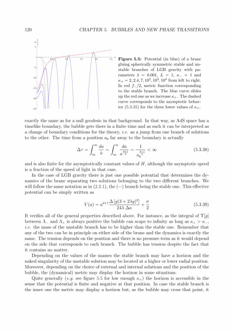
120 CHAPTER 5. BUBBLES AND NEW PHASE TRANSITIONS
0.5 1.0 1.5 2.0 2.5a
-25
-20
-15
-10
-5
5
V,f
-
2
Figure 5.5: Potential (in blue) of a branegluing spherically symmetric stable and un-stable branches of LGB gravity with pa-rameters λ = 0.001, L = 1, κ− = 1 andκ+ = 2, 2.4, 7, 102, 103, 104 from left to right.In red f−/2, metric function correspondingto the stable branch. The blue curve slidesup the red one as we increase κ+. The dashedcurve corresponds to the asymptotic behav-ior (5.3.35) for the three lower values of κ+.
exactly the same as for a null geodesic in that background. In that way, as AdS space has atimelike boundary, the bubble gets there in a finite time and as such it can be interpreted asa change of boundary conditions for the theory, i.e. as a jump from one branch of solutionsto the other. The time from a position a0 far away to the boundary is actually
∆τ =
∫ ∞a0
da
a∼∫ ∞a0
da
ad+1
2
∼ 1
ad−1
20
<∞ (5.3.38)
and is also finite for the asymptotically constant values of H, although the asymptotic speedis a fraction of the speed of light in that case.
In the case of LGB gravity there is just one possible potential that determines the dy-namics of the brane separating two solutions belonging to the two different branches. Wewill follow the same notation as in (2.2.1), the (−) branch being the stable one. This effectivepotential can be simply written as
V (a) = ad+1 ∆ [g(3 + 2λg)2]
24λ ∆κ+σ
2(5.3.39)
It verifies all of the general properties described above. For instance, as the integral of Υ[g]between Λ− and Λ+ is always positive the bubble can scape to infinity as long as κ+ > κ−,i.e. the mass of the unstable branch has to be higher than the stable one. Remember thatany of the two can be in principle on either side of the brane and the dynamics is exactly thesame. The tension depends on the position and there is no pressure term as it would dependon the side that corresponds to each branch. The bubble has tension despite the fact thatit contains no matter.
Depending on the values of the masses the stable branch may have a horizon and thenaked singularity of the unstable solution may be located at a higher or lower radial position.Moreover, depending on the choice of external and internal solutions and the position of thebubble, the (dynamical) metric may display the horizon in some situations.
Quite generally (e.g. see figure 5.5 for low enough κ+) the horizon is accessible in thesense that the potential is finite and negative at that position. In case the stable branch isthe inner one the metric may display a horizon but, as the bubble may cross that point, it
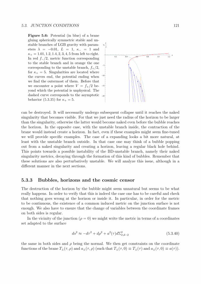
5.3. JUNCTION CONDITIONS 121
Figure 5.6: Potential (in blue) of a branegluing spherically symmetric stable and un-stable branches of LGB gravity with param-eters λ = −0.01, L = 1, κ− = 1 andκ+ = 1.01, 1.2, 1.4, 2, 3, 4, 5 from left to right.In red f−/2, metric function correspondingto the stable branch and in orange the onecorresponding to the unstable branch, f+/2,for κ+ = 5. Singularities are located wherethe curves end, the potential ending whenwe find the outermost of them. Before thatwe encounter a point where V = f+/2 be-yond which the potential is unphysical. Thedashed curve corresponds to the asymptoticbehavior (5.3.35) for κ+ = 5.
0.2 0.4 0.6 0.8 1.0 1.2a
-20
-15
-10
-5
V,f
-
2
can be destroyed. It will necessarily undergo subsequent collapse until it reaches the nakedsingularity that becomes visible. For that we just need the radius of the horizon to be largerthan the singularity, otherwise the latter would become naked even before the bubble reachesthe horizon. In the opposite case, with the unstable branch inside, the contraction of thebrane would instead create a horizon. In fact, even if these examples might seem fine-tunedwe will provide specific examples. The case of a expanding looks a bit more natural, atleast with the unstable branch outside. In that case one may think of a bubble poppingout from a naked singularity and creating a horizon, leaving a regular black hole behind.This points towards a possible instability of the BD-unstable branch, namely their nakedsingularity metrics, decaying through the formation of this kind of bubbles. Remember thatthese solutions are also perturbatively unstable. We will analyze this issue, although in adifferent manner in the next sections.
5.3.3 Bubbles, horizons and the cosmic censor
The destruction of the horizon by the bubble might seem unnatural but seems to be whatreally happens. In order to verify that this is indeed the case one has to be careful and checkthat nothing goes wrong at the horizon or inside it. In particular, in order for the metricto be continuous, the existence of a common induced metric on the junction surface is notenough. We also have to ensure that the change of variables between the coordinate frameson both sides is regular.
In the vicinity of the junction (ρ = 0) we might write the metric in terms of a coordinatesset adapted to the surface
ds2 ≈ −dτ 2 + dρ2 + a2(τ)dΣ2σ,d−2 (5.3.40)
the same in both sides and ρ being the normal. We then get constraints on the coordinatefunctions of the brane T±(τ, ρ) and a±(τ, ρ) (such that T±(τ, 0) ≡ T±(τ) and a±(τ, 0) ≡ a(τ)).
122 CHAPTER 5. BUBBLES AND NEW PHASE TRANSITIONS
One is the Lorentzian analogue of the previously found (5.3.13) and additionally,
− f±T ′2± +a′2±f±
= 1 ; −f±T ′±T± +a′±a±f±
= 0 (5.3.41)
where primes indicate derivatives with respect to the new variable ρ. Remark that the radialvariables are not equal in this case even though they are at the junction.
In this way we may write the change of variables as
dt± = T± dτ +a
f±dρ
dr± = a dτ + f±T±dρ (5.3.42)
that corresponds to a boost in the (t±, r±)-plane. This can be easily verified using theorthonormal frame (2.1.5) e0
±
e1±
= U±
dτ
dρ
U± =
√f±T±
a√f±
a√f±
√f±T±
. (5.3.43)
the boost matrix having unit determinant with an inverse obtained just by changing the signof a. Remember that T± can be written in terms of a using (5.3.13), being invariant underthat change. The change of variables between inner and outer coordinates corresponds thusto a composition of boosts e+ = U+U
−1− e−, a transformation that does not change the causal
structure, i.e. null geodesics are continuous across the bubble.We can now address the question of the behavior of the bubble as we cross the horizon.
In that case we have to change√f− = i
√‖f−‖, as f− goes negative, in such a way that the
timelike and spacelike vielbeine exchange their roles2 preserving the orientation (e0− ∧ e1
− =e0− ∧ e1
−)e0− = ie1
− ; e1− = ie0
− . (5.3.45)
Consequently the change of variables behind the horizon e0−
e1−
= U−
dτ
dρ
U− =1√‖f−‖
−a −√f− + a2
−√f− + a2 −a
. (5.3.46)
again corresponds to a boost and is completely well defined. The change is actually continu-ous across the horizon, the bubble being able to cross it. After all there is nothing special –locally – about that point. Besides, once it gets to the horizon the causal structure makes itimpossible for the bubble to get back (see figure 4.3 for the Penrose diagram of the process)as it would be travelling backwards in time. This can also be seen from (5.3.46) as the
2Inside the horizon
e0 = − dr√‖f‖
; e1 =√‖f‖dt (5.3.44)
5.4. THERMALONS AND THERMODYNAMICS 123
diagonal components of the U− matrix have to be positive and bigger than one. This is alsotrue for U± outside the horizon.
It is remarkable that, even though the original horizon is destroyed by the bubble thecausal structure inherited by it makes it impossible for the bubble to go back. In this casewe cannot blame the symmetry of the solutions considered as we did in chapter 4. Oncethe horizon is crossed, its (previous) presence forces the bubble to actually reach the centralsingularity, regardless of the details of the collapse. The singularity unavoidably becomesnaked, this being a clear violation of the cosmic censorship hypothesis. Nonetheless, thisviolation might be a marginal one if, due to the instabilities suffered by those singularsolutions (see chapter 4 for details), the energy leaks the singularity, thus leaving regularpure AdS+ behind. This process is allowed by the causal structure of the spacetime. Noticethat the bubble itself may also emit part of its mass, M +−M−, to infinity before it actuallyreaches the singularity. However the naked singularity will still form as the mass containedin the inner solution, M−, cannot scape until the bubble reaches the center.
5.4 Thermalons and thermodynamics
Bubble configurations when static are subject to the same discussion of chapter 3, concerningthe thermodynamics aspects of black holes. In very much the same way, the new solutionswill be characterized by the same thermodynamic variables.
In this section we will compute the value of the Euclidean on-shell action for thesethermalons. Such static solutions will exist in some cases as it can be seen in figure 5.5for the case of LGB gravity with positive λ coupling. Being static, they trivially have asmooth Euclidean section whenever they display a horizon in the inner solution coveringthe singularity. We have to choose the periodicity in Euclidean time accordingly, so thatthe full configuration is smooth. Once the inner periodicity is fixed to attain a regularhorizon, the periodicity in the outer time will be determined through (5.3.15), thus fixingthe temperature.
As for black holes, the Euclidean on-shell action is in general divergent and needs tobe regularized, either by background substraction or by other means. We will measure thefree energy with respect to the specific solution used as groundstate, usually the maximallysymmetric one. In order to simplify the discussion we will calculate the on-shell actionin terms of three parameters, a? and β±, the first being the equilibrium position of thebubble and the others the periodicity in Euclidean time in the inner and outer regions. Itis important to keep in mind that these two variables are not independent from each other.We will use + to denote the outer region and − for the inner one. This is more general but itwill be consistent with the notation of the LGB branches when we undertake that analysis.
Unlike the computation of the Hawking-Page effect described in section 3, where thefields are continuous, here we have to consider the contribution to the action arising on thebubble, when writing the Euclidean action in the form (5.3.8),
I = I− + IΣ + I+ . (5.4.1)
The outer piece includes all the boundary terms at infinity necessary to both have a welldefined variational principle. It regularizes its divergence by subtracting the background
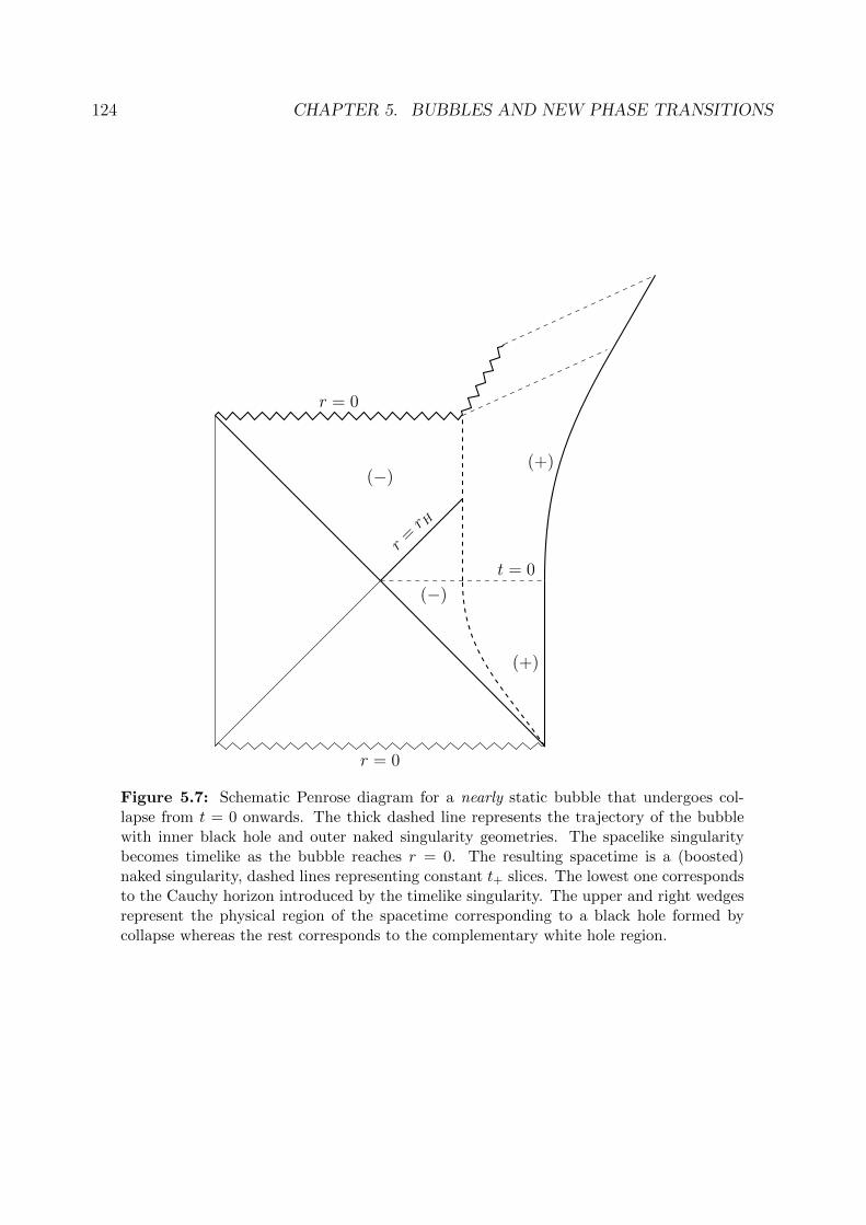
124 CHAPTER 5. BUBBLES AND NEW PHASE TRANSITIONS
(−)
(+)
r=rH
r = 0
r = 0
(+)
(−)
t = 0
Figure 5.7: Schematic Penrose diagram for a nearly static bubble that undergoes col-lapse from t = 0 onwards. The thick dashed line represents the trajectory of the bubblewith inner black hole and outer naked singularity geometries. The spacelike singularitybecomes timelike as the bubble reaches r = 0. The resulting spacetime is a (boosted)naked singularity, dashed lines representing constant t+ slices. The lowest one correspondsto the Cauchy horizon introduced by the timelike singularity. The upper and right wedgesrepresent the physical region of the spacetime corresponding to a black hole formed bycollapse whereas the rest corresponds to the complementary white hole region.
5.4. THERMALONS AND THERMODYNAMICS 125
M+ = 0 with the same periodicity at infinity, yielding
I+(a?, β+) = β+(d− 2)Vd−2
16πGN
∂r
[rd Υ[g+]
]∣∣∣a?, (5.4.2)
that has the same expression as for the usual black holes (3.2.2) evaluated at the position of
the bubble instead of the horizon. The term I−, in turn, is integrated from the horizon tothe location of the bubble yielding two terms of the same form, one evaluated on the bubbleand one at the horizon.
I−(a?, β−) = β−(d− 2)Vd−2
16πGN
(∂r
[rd Υ[g−]
]∣∣∣rH− ∂r
[rd Υ[g−]
]∣∣∣a?
). (5.4.3)
where rH is the radius of the horizon, if any, or zero. Finally, IΣ is given by
IΣ = −I−∂ (a?, β0) + I+∂ (a?, β0) (5.4.4)
where the periodicity in Euclidean time is inherited from the bulk regions β0 =√f±(a)β±.
Then, we can collect all the contributions that depend upon the location of the bubble,
Ibub(a?, β0) = β0(d− 2)Vd−2
16πGN
(1√f∂r
[rd Υ[g]
]∣∣∣a?
+ 2 ∂r
[rd−2
√f
∫ 1
0
dt Υ′[(1− t2)gH + t2 g
]]∣∣∣∣a?
)∣∣∣∣+−
(5.4.5)
in the static case, otherwise we cannot perform the τ integration, and where F(g)|+− =F(g+) − F(g−), indicates the difference between the terms evaluated on both sides of thebrane. The rest can be consequently called
Ibh = I − Ibub = β−M− − S , (5.4.6)
the usual contribution from the inner black hole. Trivially the surface term vanishes whenthe same solution is taken in both sides of the junction.
The contribution from the bubble can be greatly simplified making use of the relationsbetween the two characteristic polynomials Υ[g] and Υ[g], as in (3.2.8), and also someproperties obtained by integrating by parts expressions of the type∫ 1
0
dtP [t2g + (1− t2)H?] = P [g] + 2(H? − g)
∫ 1
0
dt t2P ′[t2g + (1− t2)H?] (5.4.7)
Remarkably enough, a neat result comes out after a quite lengthy calculation, once thejunction conditions are imposed
Ibub =(d− 2)Vd−2
16πGN
(β+κ+ − β−κ−) = β+M+ − β−M− (5.4.8)
which is the exact value needed to correct the on-shell action in such a way that the ther-modynamic interpretation is safely preserved. In fact, because of this contribution, the totalaction takes the form
I = Ibh + Ibub = β+M+ − S . (5.4.9)
126 CHAPTER 5. BUBBLES AND NEW PHASE TRANSITIONS
That is, the brane contributes as mass (it carries the mass difference between the two solu-tions) but not as entropy that comes solely from the horizon. From the Hamiltonian point ofview this is naturally understood as follows. The canonical action vanishes in this case, theonly possible contributions coming from boundary terms both at infinity and at the horizon,yielding respectively β+M+ and the entropy, which are nothing but the total charges of thesolution.
For the above result we have just imposed the first junction condition, Π[g?±, H?] = 0,where H? = σ/a2
? is the static value of H. The other junction condition corresponds to theradial derivative of the first one in such a way that
∂aΠ[g?±, H?] = ∂g+Π[g?±, H?] g′+
∣∣?
+ ∂g−Π[g±, H?] g′−∣∣?
+ ∂HΠ[g±, H?]H′? = 0 . (5.4.10)
The H derivative of Π plays another fundamental role as it gives the overall normalizationof the effective potential (see discussion above). Using (5.3.25) we can show
∂g±Π[g±, H?] =−1
2√H? − g?±
Υ′[g?±] . (5.4.11)
Also for the other derivative after a bit of massage we get
∂H(Π+ − Π−
)= −1
2
∫ √H?−g+
√H?−g−
dxΥ′[H? − x2]
x2(5.4.12)
Then, using the black hole equation (2.1.8), we can write the second junction condition as
κ+√f+
− κ−√f−
=4σ
d− 1ad−4∂HΠ[g±, H?] (5.4.13)
Notice that the left hand side of this expression is proportional to the contribution of thebubble (5.4.5) to the on-shell action (or equivalently the free energy).
This junction condition is also very important to ensure a consistent thermodynamicpicture. We have seen in the previous paragraphs that the on-shell action adopts the expectedform from the semi-classical approach (5.4.9) where the different quantities correspond tothe expected ones in the solution, i.e.
β = β+ , M = M+ , (5.4.14)
the entropy being unchanged as coming from the inner black hole horizon. In order toshow the consistency of the thermodynamics in addition to this the relations between thisquantities and the corresponding thermodynamic potentials should be also the correct ones,as seen in 3. It is enough to show that assuming the above values for mass and entropy werecover the correct temperature as
T =dM
dS=dM+
da?
da?drH
drHdS
(5.4.15)
where we have to use the implicit relation between the two parameters involved, a? and rH
κ−(a?) = rd−1H Υ
[σ
r2H
]. (5.4.16)
5.4. THERMALONS AND THERMODYNAMICS 127
Equivalently we can use the property
dS = β−dM− (5.4.17)
so that the inverse temperature is
β =dS
dM= β−
dM−dM+
. (5.4.18)
In order for this to be equal to β+ as required we must verify
β+dM+ = β−dM− = dS (5.4.19)
where the differential is taken with respect to the parameter a? or equivalently rH or T . Thisimplies that the first law of thermodynamics holds true not only for the inner black hole(β− and M−) but for the whole configuration (β+ and M+). This can be easily proven usingboth junction conditions. First we derive the first one with respect to a?. For that we haveto take into account that, in contrast with the differentiation of the potential with respectto a (not a?) from which we obtained the second junction condition, the mass parametersκ± depend now on the variable. The expression itself depends on κ± through g?± and so onegets
Υ[g?±] =κ±(a?)
ad−1?
⇒(g?±)′
=−(d− 1)κ± + a?κ
′±
ad?Υ′[g?±]
(5.4.20)
The final result is the same as obtained for the second junction condition with an extra termproportional to the derivatives of the mass parameters, κ±,
κ+ + aκ′+√f+
−κ+ + aκ′+√
f−=
4σ
d− 1ad−4∂HΠ[g?±, H?] . (5.4.21)
Then, the term proportional to the mass parameter cancels the right hand side of the equationand we get just
κ′+√f+
−κ′+√f−
= 0 (5.4.22)
that multiplied by β0 yields (5.4.19) that is exactly what we were looking for.We have shown that the first law of thermodynamics holds for the whole bubble config-
uration whereas the thermodynamic parameters verify the expected relations, this provingthe consistency of the thermodynamic approach. Having computed the free energy of thisgeometry, we can now compare it to the rest of the solutions sharing the same boundary con-ditions and temperature and thus identify the preferred or classical configuration as the oneof lower free energy. We can also analyze the local thermodynamic stability of the solutionsas we did for the black hole solutions in chapter 3.
5.4.1 LGB thermalons
Before analyzing the free energy of the thermalon configurations and the occurrence of phasetransitions let us describe a bit in more detail the configurations we are dealing with in the
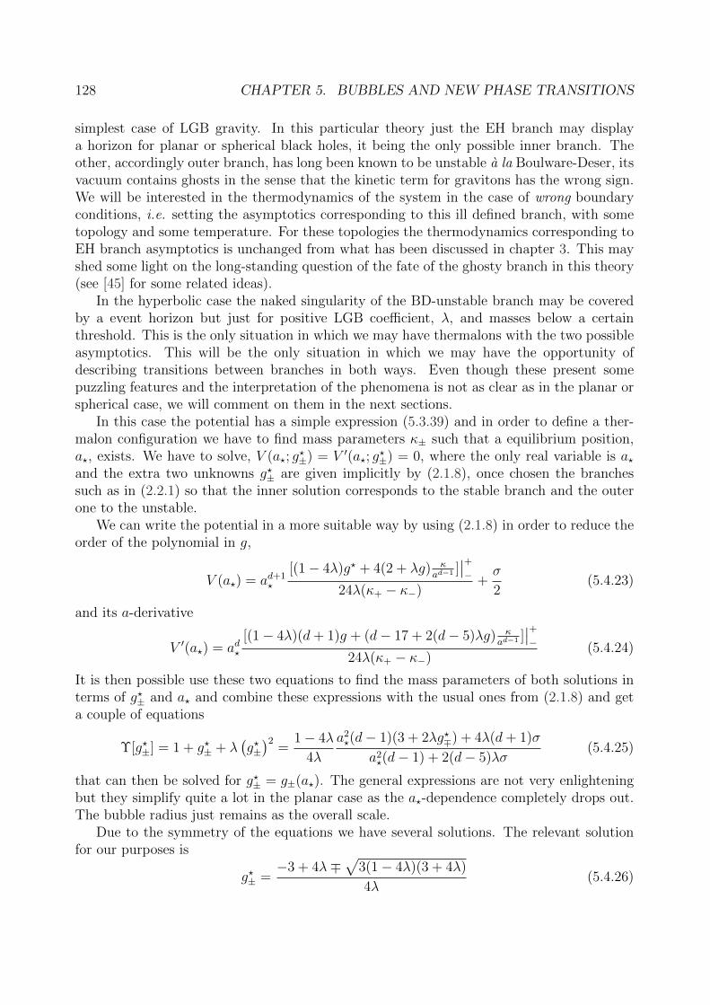
128 CHAPTER 5. BUBBLES AND NEW PHASE TRANSITIONS
simplest case of LGB gravity. In this particular theory just the EH branch may displaya horizon for planar or spherical black holes, it being the only possible inner branch. Theother, accordingly outer branch, has long been known to be unstable a la Boulware-Deser, itsvacuum contains ghosts in the sense that the kinetic term for gravitons has the wrong sign.We will be interested in the thermodynamics of the system in the case of wrong boundaryconditions, i.e. setting the asymptotics corresponding to this ill defined branch, with sometopology and some temperature. For these topologies the thermodynamics corresponding toEH branch asymptotics is unchanged from what has been discussed in chapter 3. This mayshed some light on the long-standing question of the fate of the ghosty branch in this theory(see [45] for some related ideas).
In the hyperbolic case the naked singularity of the BD-unstable branch may be coveredby a event horizon but just for positive LGB coefficient, λ, and masses below a certainthreshold. This is the only situation in which we may have thermalons with the two possibleasymptotics. This will be the only situation in which we may have the opportunity ofdescribing transitions between branches in both ways. Even though these present somepuzzling features and the interpretation of the phenomena is not as clear as in the planar orspherical case, we will comment on them in the next sections.
In this case the potential has a simple expression (5.3.39) and in order to define a ther-malon configuration we have to find mass parameters κ± such that a equilibrium position,a?, exists. We have to solve, V (a?; g
?±) = V ′(a?; g
?±) = 0, where the only real variable is a?
and the extra two unknowns g?± are given implicitly by (2.1.8), once chosen the branchessuch as in (2.2.1) so that the inner solution corresponds to the stable branch and the outerone to the unstable.
We can write the potential in a more suitable way by using (2.1.8) in order to reduce theorder of the polynomial in g,
V (a?) = ad+1?
[(1− 4λ)g? + 4(2 + λg) κad−1 ]
∣∣+−
24λ(κ+ − κ−)+σ
2(5.4.23)
and its a-derivative
V ′(a?) = ad?[(1− 4λ)(d+ 1)g + (d− 17 + 2(d− 5)λg) κ
ad−1 ]∣∣+−
24λ(κ+ − κ−)(5.4.24)
It is then possible use these two equations to find the mass parameters of both solutions interms of g?± and a? and combine these expressions with the usual ones from (2.1.8) and geta couple of equations
Υ[g?±] = 1 + g?± + λ(g?±)2
=1− 4λ
4λ
a2?(d− 1)(3 + 2λg?∓) + 4λ(d+ 1)σ
a2?(d− 1) + 2(d− 5)λσ
(5.4.25)
that can then be solved for g?± = g±(a?). The general expressions are not very enlighteningbut they simplify quite a lot in the planar case as the a?-dependence completely drops out.The bubble radius just remains as the overall scale.
Due to the symmetry of the equations we have several solutions. The relevant solutionfor our purposes is
g?± =−3 + 4λ∓
√3(1− 4λ)(3 + 4λ)
4λ(5.4.26)
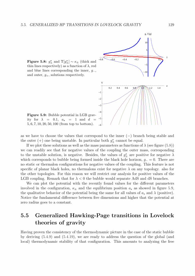
5.5. GENERALIZED HP TRANSITIONS IN LOVELOCK GRAVITY 129
Figure 5.8: g?± and Υ[g?±] ∼ κ± (thick andthin lines respectively) as a function of λ, redand blue lines corresponding the inner, g−,and outer, g+, solutions respectively.
-0.8 -0.6 -0.4 -0.2 0.2Λ
-10
-5
5
10
g, U@gD
Figure 5.9: Bubble potential in LGB grav-ity for λ = 0.1, a? = 1 and d =5, 6, 7, 10, 20, 50, 100 (from top to bottom).
0.2 0.4 0.6 0.8 1.0 1.2 1.4a
-6
-5
-4
-3
-2
-1
V
as we have to choose the values that correspond to the inner (−) branch being stable andthe outer (+) one being unstable. In particular both g?± cannot be equal.
If we plot these solutions as well as the mass parameters as functions of λ (see figure (5.8))we can readily see that for negative values of the coupling the outer mass, correspondingto the unstable solution, is negative. Besides, the values of g?± are positive for negative λwhich corresponds to bubble being formed inside the black hole horizon, g− = 0. There areno static or thermalon configurations for negative values of the coupling. This feature is notspecific of planar black holes, no thermalons exist for negative λ on any topology. also forthe other topologies. For this reason we will restrict our analysis for positive values of theLGB coupling. Remark that for λ < 0 the bubble would separate AdS and dS branches.
We can plot the potential with the recently found values for the different parametersinvolved in the configuration, κ± and the equilibrium position a? as showed in figure 5.9,the qualitative behavior of the potential being the same for all values of a? and λ (positive).Notice the fundamental difference between five dimensions and higher that the potential atzero radius goes to a constant.
5.5 Generalized Hawking-Page transitions in Lovelock
theories of gravity
Having proven the consistency of the thermodynamic picture in the case of the static bubbleby deriving (5.4.9) and (5.4.19), we are ready to address the question of the global (andlocal) thermodynamic stability of that configuration. This amounts to analyzing the free
130 CHAPTER 5. BUBBLES AND NEW PHASE TRANSITIONS
energy associated to that solution, the analysis being analogous to that of section 3.5. Theonly difference is that we now need to include the thermalons discussed above. This willallow for the study of the formation of these new configurations and the consequences forthe dynamics of the system.
In the same way as for the usual Hawking-Page phase transition we can identify the ther-modynamically preferred or classical configuration as the background of least on-shell actionamong all those with a smooth Euclidean continuation and the same period in imaginarytime.
The first example that can be trivially analyzed is that of planar black holes in generalLovelock gravity. In this case the only branch displaying a horizon, as already discussedin the previous sections, is the EH one, all the others being unstable and displaying nakedsingularities. Because of that, the only possible smooth Euclidean metrics correspond to thevacua of the theory and bubble configurations with the inner region corresponding to the EHbranch. Then, for any choice of asymptotics (different from EH), the configurations we willbe comparing are corresponding thermal vacuum and, when available, the horizonful bubbleconfiguration with the same temperature.
The junction conditions simplify a lot in this case, the free energy corresponding just tothe black hole with no bubble contribution. The presence of the junction plays no role exceptfor the change on the temperature according to (5.3.15). The free energy of the thermalvacuum is zero, as we have taken it as reference background, and that of the thermalonyields
F+ =IEβ+
=β−β+
F− = − M+
d− 2, (5.5.1)
which is always negative. This implies that the preferable classical solution is, when available,the thermalon. One of them if there are several with the same asymptotics. For any branchof solutions such that the planar thermalon with the inner EH branch exists, the bubble willalways form. Remember that β−M− = β+M+ and the inner mass has to be positive in orderto have a horizon.
In the LGB case the thermalon exists just for positive λ, the equilibrium position be-ing unstable. It will therefore eventually expand in such a way that it engulfs the wholespacetime in finite proper time, thus changing its asymptotic behavior (and the associatedthermodynamic variables) [5].
In the planar case the problem of the existence of these kind of configurations translatesinto finding couples g?± that verify the static junction equations, that can be written as
Υ[g?]√−g?
∣∣∣∣+−
= 0 ;
∫ √−g?+√−g?−
dxΥ′[−x2] = 0 (5.5.2)
and subsequently as polynomial equations for g?±. The solutions for any Lovelock theory canbe plot, a specific example for cubic Lovelock theory being depicted in figure 5.10. Eventhough the independent variable x =
√−g is not the usual one for the polynomial, we can
easily recognize the three vacua, Υ = 0, and associated branches. These correspond tothe three ranges with definite sign for Υ′, positive for the branches that are stable (a laBoulware-Deser) and negative for the intermediate unstable one. The EH branch is the one
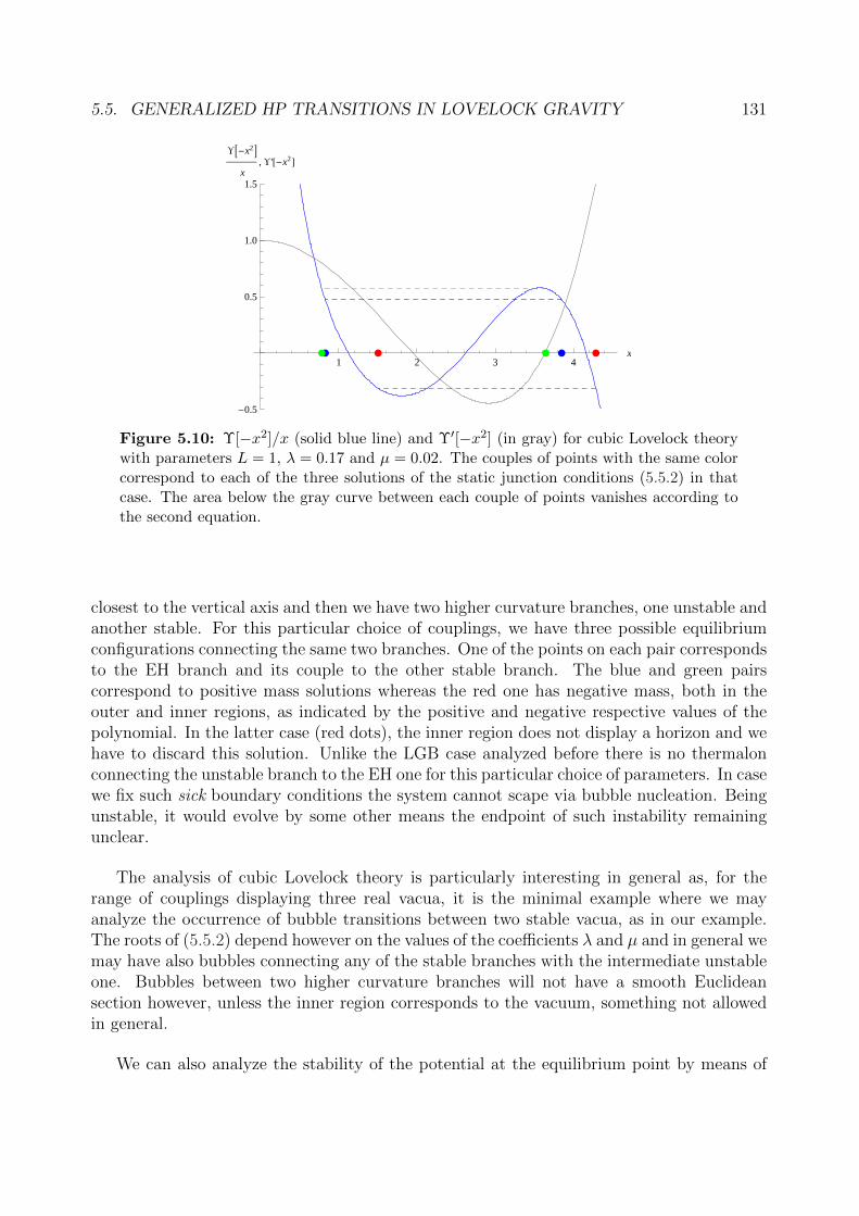
5.5. GENERALIZED HP TRANSITIONS IN LOVELOCK GRAVITY 131
1 2 3 4x
-0.5
0.5
1.0
1.5
UA-x2E
x, U'@-x2D
Figure 5.10: Υ[−x2]/x (solid blue line) and Υ′[−x2] (in gray) for cubic Lovelock theorywith parameters L = 1, λ = 0.17 and µ = 0.02. The couples of points with the same colorcorrespond to each of the three solutions of the static junction conditions (5.5.2) in thatcase. The area below the gray curve between each couple of points vanishes according tothe second equation.
closest to the vertical axis and then we have two higher curvature branches, one unstable andanother stable. For this particular choice of couplings, we have three possible equilibriumconfigurations connecting the same two branches. One of the points on each pair correspondsto the EH branch and its couple to the other stable branch. The blue and green pairscorrespond to positive mass solutions whereas the red one has negative mass, both in theouter and inner regions, as indicated by the positive and negative respective values of thepolynomial. In the latter case (red dots), the inner region does not display a horizon and wehave to discard this solution. Unlike the LGB case analyzed before there is no thermalonconnecting the unstable branch to the EH one for this particular choice of parameters. In casewe fix such sick boundary conditions the system cannot scape via bubble nucleation. Beingunstable, it would evolve by some other means the endpoint of such instability remainingunclear.
The analysis of cubic Lovelock theory is particularly interesting in general as, for therange of couplings displaying three real vacua, it is the minimal example where we mayanalyze the occurrence of bubble transitions between two stable vacua, as in our example.The roots of (5.5.2) depend however on the values of the coefficients λ and µ and in general wemay have also bubbles connecting any of the stable branches with the intermediate unstableone. Bubbles between two higher curvature branches will not have a smooth Euclideansection however, unless the inner region corresponds to the vacuum, something not allowedin general.
We can also analyze the stability of the potential at the equilibrium point by means of
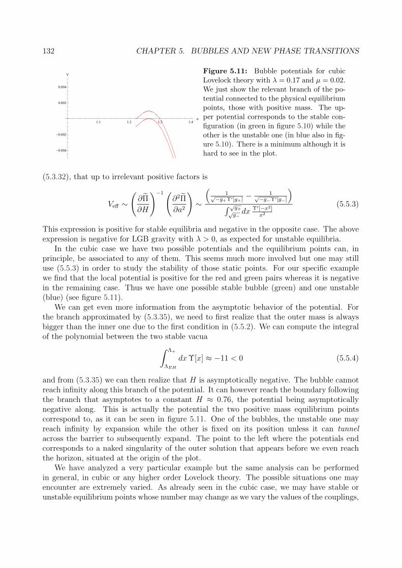
132 CHAPTER 5. BUBBLES AND NEW PHASE TRANSITIONS
1.1 1.2 1.3 1.4a
-0.004
-0.002
0.002
0.004
VFigure 5.11: Bubble potentials for cubicLovelock theory with λ = 0.17 and µ = 0.02.We just show the relevant branch of the po-tential connected to the physical equilibriumpoints, those with positive mass. The up-per potential corresponds to the stable con-figuration (in green in figure 5.10) while theother is the unstable one (in blue also in fig-ure 5.10). There is a minimum although it ishard to see in the plot.
(5.3.32), that up to irrelevant positive factors is
Veff ∼
(∂Π
∂H
)−1(∂2Π
∂a2
)∼
(1√
−g+Υ′[g+]− 1√
−g−Υ′[g−]
)∫ √g+√
g−dx Υ′[−x2]
x2
(5.5.3)
This expression is positive for stable equilibria and negative in the opposite case. The aboveexpression is negative for LGB gravity with λ > 0, as expected for unstable equilibria.
In the cubic case we have two possible potentials and the equilibrium points can, inprinciple, be associated to any of them. This seems much more involved but one may stilluse (5.5.3) in order to study the stability of those static points. For our specific examplewe find that the local potential is positive for the red and green pairs whereas it is negativein the remaining case. Thus we have one possible stable bubble (green) and one unstable(blue) (see figure 5.11).
We can get even more information from the asymptotic behavior of the potential. Forthe branch approximated by (5.3.35), we need to first realize that the outer mass is alwaysbigger than the inner one due to the first condition in (5.5.2). We can compute the integralof the polynomial between the two stable vacua∫ Λ+
ΛEH
dxΥ[x] ≈ −11 < 0 (5.5.4)
and from (5.3.35) we can then realize that H is asymptotically negative. The bubble cannotreach infinity along this branch of the potential. It can however reach the boundary followingthe branch that asymptotes to a constant H ≈ 0.76, the potential being asymptoticallynegative along. This is actually the potential the two positive mass equilibrium pointscorrespond to, as it can be seen in figure 5.11. One of the bubbles, the unstable one mayreach infinity by expansion while the other is fixed on its position unless it can tunnelacross the barrier to subsequently expand. The point to the left where the potentials endcorresponds to a naked singularity of the outer solution that appears before we even reachthe horizon, situated at the origin of the plot.
We have analyzed a very particular example but the same analysis can be performedin general, in cubic or any higher order Lovelock theory. The possible situations one mayencounter are extremely varied. As already seen in the cubic case, we may have stable orunstable equilibrium points whose number may change as we vary the values of the couplings,
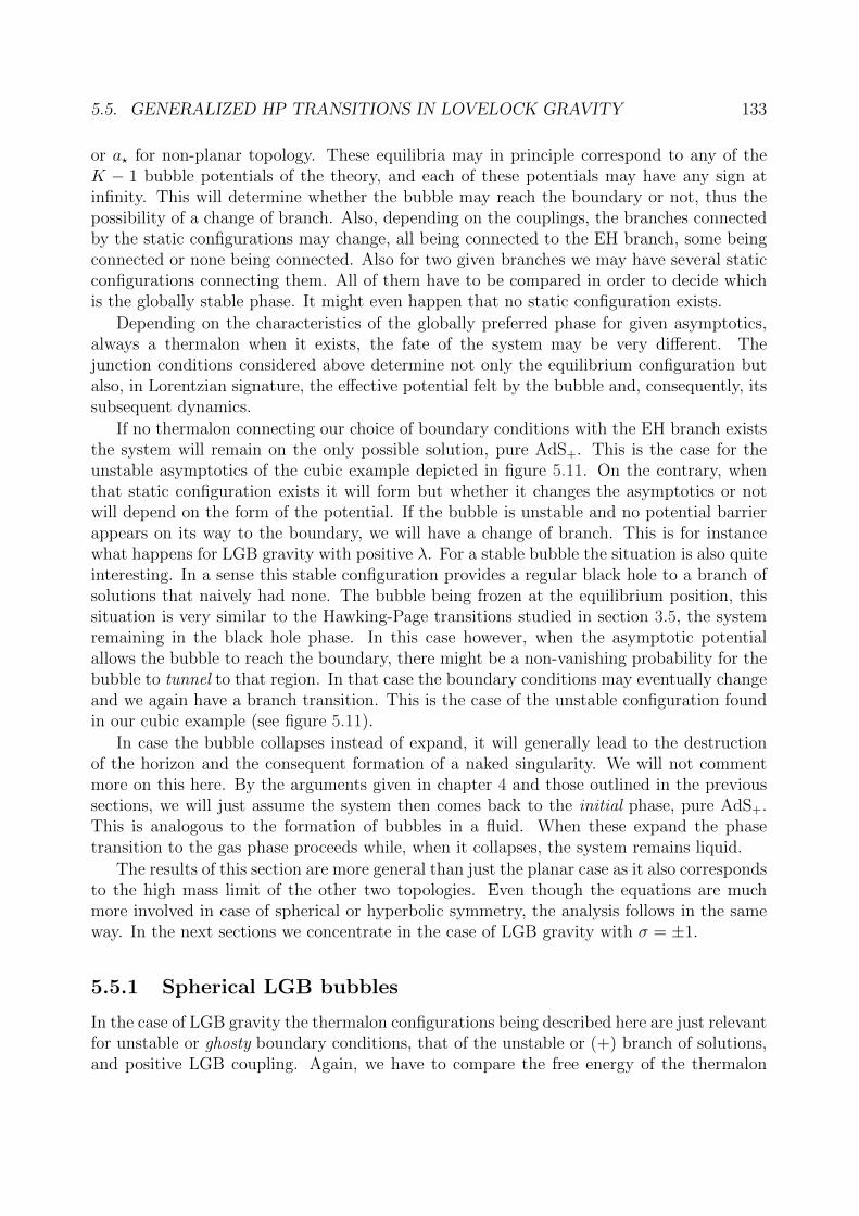
5.5. GENERALIZED HP TRANSITIONS IN LOVELOCK GRAVITY 133
or a? for non-planar topology. These equilibria may in principle correspond to any of theK − 1 bubble potentials of the theory, and each of these potentials may have any sign atinfinity. This will determine whether the bubble may reach the boundary or not, thus thepossibility of a change of branch. Also, depending on the couplings, the branches connectedby the static configurations may change, all being connected to the EH branch, some beingconnected or none being connected. Also for two given branches we may have several staticconfigurations connecting them. All of them have to be compared in order to decide whichis the globally stable phase. It might even happen that no static configuration exists.
Depending on the characteristics of the globally preferred phase for given asymptotics,always a thermalon when it exists, the fate of the system may be very different. Thejunction conditions considered above determine not only the equilibrium configuration butalso, in Lorentzian signature, the effective potential felt by the bubble and, consequently, itssubsequent dynamics.
If no thermalon connecting our choice of boundary conditions with the EH branch existsthe system will remain on the only possible solution, pure AdS+. This is the case for theunstable asymptotics of the cubic example depicted in figure 5.11. On the contrary, whenthat static configuration exists it will form but whether it changes the asymptotics or notwill depend on the form of the potential. If the bubble is unstable and no potential barrierappears on its way to the boundary, we will have a change of branch. This is for instancewhat happens for LGB gravity with positive λ. For a stable bubble the situation is also quiteinteresting. In a sense this stable configuration provides a regular black hole to a branch ofsolutions that naively had none. The bubble being frozen at the equilibrium position, thissituation is very similar to the Hawking-Page transitions studied in section 3.5, the systemremaining in the black hole phase. In this case however, when the asymptotic potentialallows the bubble to reach the boundary, there might be a non-vanishing probability for thebubble to tunnel to that region. In that case the boundary conditions may eventually changeand we again have a branch transition. This is the case of the unstable configuration foundin our cubic example (see figure 5.11).
In case the bubble collapses instead of expand, it will generally lead to the destructionof the horizon and the consequent formation of a naked singularity. We will not commentmore on this here. By the arguments given in chapter 4 and those outlined in the previoussections, we will just assume the system then comes back to the initial phase, pure AdS+.This is analogous to the formation of bubbles in a fluid. When these expand the phasetransition to the gas phase proceeds while, when it collapses, the system remains liquid.
The results of this section are more general than just the planar case as it also correspondsto the high mass limit of the other two topologies. Even though the equations are muchmore involved in case of spherical or hyperbolic symmetry, the analysis follows in the sameway. In the next sections we concentrate in the case of LGB gravity with σ = ±1.
5.5.1 Spherical LGB bubbles
In the case of LGB gravity the thermalon configurations being described here are just relevantfor unstable or ghosty boundary conditions, that of the unstable or (+) branch of solutions,and positive LGB coupling. Again, we have to compare the free energy of the thermalon
134 CHAPTER 5. BUBBLES AND NEW PHASE TRANSITIONS
0.00 0.05 0.10 0.15 0.20 0.25Λ0
2
4
6
8
10
12
14
Tc
2 4 6 8 10 12T0.0
0.1
0.2
0.3
0.4F
Figure 5.12: Free energy versus tempera-ture in 5d for λ = 0.04, 0.06, 0.09 (positiv-ity bound), 0.219 (maximal F (T = 0)), andλ → 1/4 (from right to left). The λ depen-dence of the critical temperature is displayedin a separate box.
configurations found in the preceding sections with the corresponding thermal vacuum. Fromthe Euclidean point of view this is the only other smooth metric with that unstable boundaryconditions.
The resulting phase diagram is similar to the usual Hawking-Page phase transition. Forany value of the LGB coupling, the free energy, F , as a function of the temperature 1/β+
displays a critical temperature above which it becomes negative and, thus, the phase transi-tion occurs (see figure 5.12). If the free energy is positive, however, the system is metastable.It decays by nucleating bubbles with a probability given, in the semiclassical approximationby e−β+F . Therefore, after enough time, the system will always end up in the stable, EHblack hole solution. This is reminiscent of the HP transition, except for the fact that, here,the thermal AdS vacuum decays into a black hole belonging to a different branch. Tc(λ)is monotonically decreasing, the phase transition becoming increasingly unlikely the morewe come closer to the EH – classical – limit. In this sense, it is a quantum mechanicalphenomenon.
5.5.2 Hyperbolic LGB bubbles
Asymptotically AdS spacetimes with hyperbolic topology are an interesting playground forchecking various facts about the recently discovered type of phase transitions. Despite someunclear features of the thermodynamics of these spacetimes, they allow in particular forthe discussion of transitions between two asymptotically AdS branches both having regularhorizonful black hole solutions. In particular, for the simplest case of LGB theory withλ > 0, both, the EH and the ghosty branch black holes, may have horizons depending onthe value of the mass. Even more, even though the range of masses for the ghosty branchis bounded from above (and below) this branch has black hole solutions for all possibletemperatures. Besides, although one of the branches is unstable we would like to investigateif the discovered transition protects the theory against this instability in the sense that theunstable branch would never be the preferred phase. This is actually the case for LGB theorywith planar or spherical symmetry. Despite the fact that the vacuum is preferred for some
5.5. GENERALIZED HP TRANSITIONS IN LOVELOCK GRAVITY 135
range of temperatures in the spherical case, the thermalon may be formed with small butfinite probability in that case leading to a change of branch.
This case is much richer, not only due to the possibility of transitions in both directions,but also because the spectrum of configurations gets richer. The existence of extremal blackholes in both branches for specific values of the mass, leads to the corresponding extremalthermalons. These extremal configurations can be considered as qualitatively different fromtheir non-extremal counterparts as regularity of the horizon in the Euclidean section doesnot fix their temperature. As a limit of non-extremal black holes the extremal solutionsnecessarily have zero temperature and the entropy corresponding to the Wald formula. Quitethe opposite, ab initio extremal configurations may be identified with any temperature andzero entropy (see chapter 3 for details). The same happens for the bubble configurations eventhough the limiting temperature is not zero. In addition to the non-extremal bubbles seen sofar there will be extremal solutions where the horizon of the inner black hole is degenerate.
For the direct transition, the one leading to the EH branch we will fix the BD-unstableasymptotics and compare the free energy of all possible configurations at the same tempera-ture. These are in principle four families of solutions, extremal and non-extremal black holesand the corresponding bubble counterparts. The same will happen for the reverse transition.
Let me first comment briefly on the thermodynamics of the unstable branch black holes.These are unstable not only a la Boulware-Deser but also thermodynamically. Their specificheat is negative and they also have negative entropy. Due to this fact their free energy willalways be bigger than the one corresponding to the extremal black hole that coincides withits mass. This extremal solution corresponds to the black hole with mass saturating theupper bound, κ = λ in five dimensions or the one corresponding to a degenerate horizon inhigher dimensions. In the 5d case the degenerate horizon coincides with the singularity atr = 0 but this does not represent a problem as that point is at the end of an infinite throatand should be removed from the geometry. The near horizon geometry can be written as
ds2 ∼ 2λdρ2 + e2ρ
(−dt
2
2λ+ dΣ2
−1,3
)(5.5.5)
where we have explicitly removed the point r = 0 considering a change of variables asρ = Logr. In higher dimensions the horizon is at finite radius and the geometry completelyregular. We will concentrate in the five dimensional case in what follows.
Thus, this particular solution is a smooth geometry interpolating between AdS5 at spatialinfinity and the previous geometry as we approach r = 0. Also, it has zero specific heat andentropy and can be considered with any periodicity in Euclidean time and thus it is a wellmotivated candidate as groundstate of the theory for the sector we are considering. Also asthe black holes are unstable all of them have higher free energy than the extremal one andthus the chosen groundstate is always preferred in a semiclassical basis. The only relevantconfiguration for the next step of the analysis will then be the extremal black hole.
We will have to compare the free energy of our thermalon configurations to that of thisgroundstate. The free energy of the non-extremal configuration has the usual expressionF = M − TS and the one corresponding to the extremal once again corresponds to aconstant, thus implying a vanishing entropy. However the extremal free energy does notcoincide with the mass in this case. In the extremal case the bubble is situated exactly
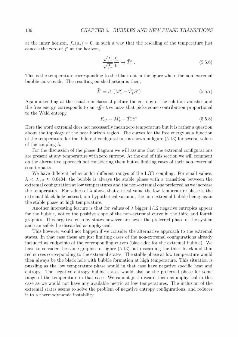
136 CHAPTER 5. BUBBLES AND NEW PHASE TRANSITIONS
at the inner horizon, f−(a?) = 0, in such a way that the rescaling of the temperature justcancels the zero of f ′ at the horizon, √
f+√f−
f ′−4π→ T e+ . (5.5.6)
This is the temperature corresponding to the black dot in the figure where the non-extremalbubble curve ends. The resulting on-shell action is then,
Ie = β+(M e+ − T e+Se) (5.5.7)
Again attending at the usual semiclassical picture the entropy of the solution vanishes andthe free energy corresponds to an effective mass that picks some contribution proportionalto the Wald entropy.
Fe,b = M e+ − T e+Se (5.5.8)
Here the word extremal does not necessarily mean zero temperature but it is rather a questionabout the topology of the near horizon region. The curves for the free energy as a functionof the temperature for the different configurations is shown in figure (5.13) for several valuesof the coupling λ.
For the discussion of the phase diagram we will assume that the extremal configurationsare present at any temperature with zero entropy. At the end of this section we will commenton the alternative approach not considering them but as limiting cases of their non-extremalcounterparts.
We have different behavior for different ranges of the LGB coupling. For small values,λ < λcrit ≈ 0.0404, the bubble is always the stable phase with a transition between theextremal configuration at low temperatures and the non-extremal one preferred as we increasethe temperature. For values of λ above that critical value the low temperature phase is theextremal black hole instead, our hypothetical vacuum, the non-extremal bubble being againthe stable phase at high temperature.
Another interesting feature is that for values of λ bigger 1/12 negative entropies appearfor the bubble, notice the positive slope of the non-extremal curve in the third and fourthgraphics. This negative entropy states however are never the preferred phase of the systemand can safely be discarded as unphysical.
This however would not happen if we consider the alternative approach to the extremalstates. In that case these are just limiting cases of the non-extremal configurations alreadyincluded as endpoints of the corresponding curves (black dot for the extremal bubble). Wehave to consider the same graphics of figure (5.13) but discarding the thick black and thinred curves corresponding to the extremal states. The stable phase at low temperature wouldthen always be the black hole with bubble formation at high temperature. This situation ispuzzling as the low temperature phase would in that case have negative specific heat andentropy. The negative entropy bubble states would also be the preferred phase for somerange of the temperature in that case. We cannot just discard them as unphysical in thiscase as we would not have any available metric at low temperatures. The inclusion of theextremal states seems to solve the problem of negative entropy configurations, and reducesit to a thermodynamic instability.
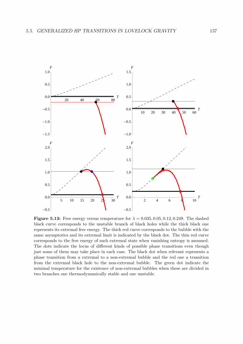
5.5. GENERALIZED HP TRANSITIONS IN LOVELOCK GRAVITY 137
20 40 60 80T
-1.5
-1.0
-0.5
0.0
0.5
1.0F
10 20 30 40 50 60T
-1.0
-0.5
0.0
0.5
1.0
1.5F
5 10 15 20 25 30T
-0.5
0.0
0.5
1.0
1.5
2.0F
2 4 6 8 10T
-0.5
0.0
0.5
1.0
1.5
2.0F
Figure 5.13: Free energy versus temperature for λ = 0.035, 0.05, 0.12, 0.249. The dashedblack curve corresponds to the unstable branch of black holes while the thick black onerepresents its extremal free energy. The thick red curve corresponds to the bubble with thesame asymptotics and its extremal limit is indicated by the black dot. The thin red curvecorresponds to the free energy of such extremal state when vanishing entropy is assumed.The dots indicate the locus of different kinds of possible phase transitions even thoughjust some of them may take place in each case. The black dot when relevant represents aphase transition from a extremal to a non-extremal bubble and the red one a transitionfrom the extremal black hole to the non-extremal bubble. The green dot indicate theminimal temperature for the existence of non-extremal bubbles when these are divided intwo branches one thermodynamically stable and one unstable.
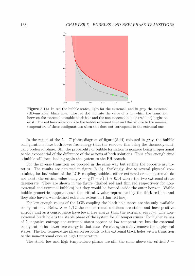
138 CHAPTER 5. BUBBLES AND NEW PHASE TRANSITIONS
0.00 0.05 0.10 0.15 0.20 0.25Λ
20
40
60
80Tcrit
Figure 5.14: In red the bubble states, light for the extremal, and in gray the extremal(BD-unstable) black hole. The red dot indicate the value of λ for which the transitionbetween the extremal unstable black hole and the non-extremal bubble (red line) begins toexist. The red line corresponds to the bubble extremal limit and the red one to the minimaltemperature of these configurations when this does not correspond to the extremal one.
In the region of the λ − T phase diagram of figure (5.14) coloured in gray, the bubbleconfigurations have both lower free energy than the vacuum, this being the thermodynami-cally preferred phase. Still the probability of bubble formation is nonzero being proportionalto the exponential of the difference of the actions of both solutions. Thus after enough timea bubble will form leading again the system to the EH branch.
For the inverse transition we proceed in the same way but setting the opposite asymp-totics. The results are depicted in figure (5.15). Strikingly, due to several physical con-straints, for low values of the LGB coupling bubbles, either extremal or non-extremal, donot exist, the critical value being λ = 1
24(7 −
√13) ≈ 0.14 where the two extremal states
degenerate. They are shown in the figure (dashed red and thin red respectively for non-extremal and extremal bubbles) but they would be formed inside the outer horizon. Viablebubble geometries appear above the critical λ value represented by the thick red line andthey also have a well-defined extremal extension (thin red line).
For low enough values of the LGB coupling the black hole states are the only availableconfigurations. Below λ = 1/12 the non-extremal solutions are stable and have positiveentropy and as a consequence have lower free energy than the extremal vacuum. The non-extremal black hole is the stable phase of the system for all temperatures. For higher valuesof λ, negative entropy non-extremal states appear at low temperatures but the extremalconfiguration has lower free energy in that case. We can again safely remove the unphysicalstates. The low temperature phase corresponds to the extremal black holes with a transitionto the non-extremal ones at high temperature.
The stable low and high temperature phases are still the same above the critical λ =
5.6. DISCUSSION 139
124
(7−√
13) where the bubble configurations appear. These can be divided in two branches,one stable that merges with the black hole curve at zero temperature and one unstable closeto the extremal state that is irrelevant as it has higher free energy than the former. Anyof these bubbles have higher free energy than the extremal black holes for all temperatures.Still and as for the transition in the other sense, the probability of a bubble being formedis nonzero and thus after enough time a bubble the BD-unstable phase would form. Thiswould in principle drive the system to that pathological branch but it is also unstable to theformation of bubbles of the EH branch. The final fate of the system seems to be a chaoticsituation with bubbles of both phases popping up everywhere. This seemingly problematicsituation is avoided for λ < 1
24(7−
√13).
In case we discard the free energy curves corresponding to the extremal states, thin redand black lines, we would encounter some problematic behavior for even lower values of λ.For λ > 1/12 negative entropy black holes appear and they would be the preferred phase forlow temperatures. Above λ = 1
24(7 −
√13) the bubbles appear with also negative entropy
and lower values of the free energy for some range of temperatures, between the lower thinred and green curves of figure (5.16).
We can summarize saying that for values of the LGB coupling below λ = 124
(7−√
13) theBD-unstable branch of hyperbolic black holes is always driven to the EH one, this being stableagainst the formation of bubbles. For this scheme the EH branch is protected and the onlytransition that takes place is a change from the extremal black hole at low temperatures tothe non-extremal at higher ones. This transition only occurs when negative entropy statesare in the spectrum, namely close to the extremal configuration. For higher values of λthe situation is chaotic with bubbles of the opposite branch popping for any choice of theboundary conditions, the interpretation of this being unclear.
Moreover, the transition mechanism presented here provides a possible resolution of theinstabilities found for the ghosty branch of LGB gravity. For spherical and planar topology itis always driven to the EH branch via bubble nucleation. We have just verified that the samehappens for hyperbolic spacetimes as long as the LGB coupling is below λ = 1
24(7 −
√13).
This will presumably be also valid in the cubic case for moderate values of µ.
5.6 Discussion
Throughout this chapter, we have broaden the scope of our analysis of Lovelock theories andtheir solutions. In particular, we have included the possibility of distributional solutions forwhich the spin connection is discontinuous at some given junction (hyper)surface. In theabsence of matter in the bubble, it glues two solutions that correspond to different branchesof the same theory, i.e. to different asymptotics. From the Hamiltonian point of view theexistence of such configurations is allowed by the multivaluedness of the canonical momenta.
We have also proven that it is possible to generalize the thermodynamic notions usuallyapplied to black holes to these new solutions. Under certain mild regularity assumptions,static bubble configurations can be assigned temperature, mass, entropy and free energy,all verifying the expected thermodynamic relations. Having proven the consistency of thethermodynamic picture, we have then analyzed local and global stability of our system inthis generalized context and the occurrence of phase transitions. We have restricted our
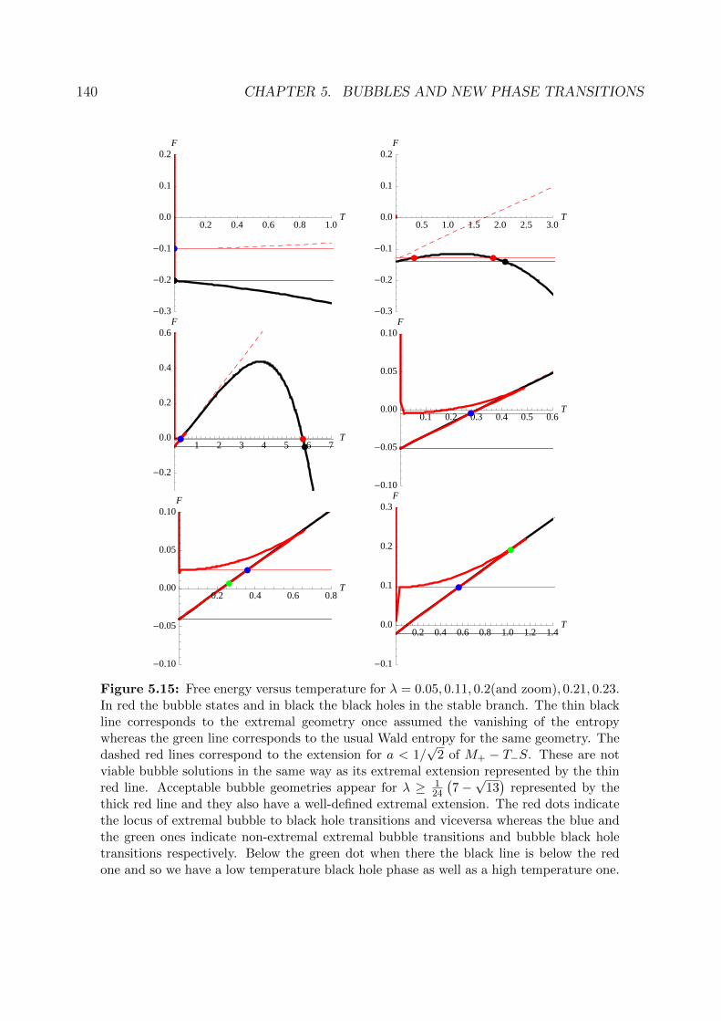
140 CHAPTER 5. BUBBLES AND NEW PHASE TRANSITIONS
0.2 0.4 0.6 0.8 1.0T
-0.3
-0.2
-0.1
0.0
0.1
0.2F
0.5 1.0 1.5 2.0 2.5 3.0T
-0.3
-0.2
-0.1
0.0
0.1
0.2F
1 2 3 4 5 6 7T
-0.2
0.0
0.2
0.4
0.6F
0.1 0.2 0.3 0.4 0.5 0.6T
-0.10
-0.05
0.00
0.05
0.10F
0.2 0.4 0.6 0.8T
-0.10
-0.05
0.00
0.05
0.10F
0.2 0.4 0.6 0.8 1.0 1.2 1.4T
-0.1
0.0
0.1
0.2
0.3F
Figure 5.15: Free energy versus temperature for λ = 0.05, 0.11, 0.2(and zoom), 0.21, 0.23.In red the bubble states and in black the black holes in the stable branch. The thin blackline corresponds to the extremal geometry once assumed the vanishing of the entropywhereas the green line corresponds to the usual Wald entropy for the same geometry. Thedashed red lines correspond to the extension for a < 1/
√2 of M+ − T−S. These are not
viable bubble solutions in the same way as its extremal extension represented by the thinred line. Acceptable bubble geometries appear for λ ≥ 1
24
(7−√
13)
represented by thethick red line and they also have a well-defined extremal extension. The red dots indicatethe locus of extremal bubble to black hole transitions and viceversa whereas the blue andthe green ones indicate non-extremal extremal bubble transitions and bubble black holetransitions respectively. Below the green dot when there the black line is below the redone and so we have a low temperature black hole phase as well as a high temperature one.
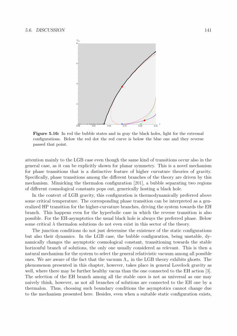
5.6. DISCUSSION 141
0.00 0.05 0.10 0.15 0.20 0.25Λ
2
4
6
8Tcrit
Figure 5.16: In red the bubble states and in gray the black holes, light for the extremalconfigurations. Below the red dot the red curve is below the blue one and they reversepassed that point.
attention mainly to the LGB case even though the same kind of transitions occur also in thegeneral case, as it can be explicitly shown for planar symmetry. This is a novel mechanismfor phase transitions that is a distinctive feature of higher curvature theories of gravity.Specifically, phase transitions among the different branches of the theory are driven by thismechanism. Mimicking the thermalon configuration [201], a bubble separating two regionsof different cosmological constants pops out, generically hosting a black hole.
In the context of LGB gravity, this configuration is thermodynamically preferred abovesome critical temperature. The corresponding phase transition can be interpreted as a gen-eralized HP transition for the higher-curvature branches, driving the system towards the EHbranch. This happens even for the hyperbolic case in which the reverse transition is alsopossible. For the EH-asymptotics the usual black hole is always the preferred phase. Belowsome critical λ thermalon solutions do not even exist in this sector of the theory.
The junction conditions do not just determine the existence of the static configurationsbut also their dynamics. In the LGB case, the bubble configuration, being unstable, dy-namically changes the asymptotic cosmological constant, transitioning towards the stablehorizonful branch of solutions, the only one usually considered as relevant. This is then anatural mechanism for the system to select the general relativistic vacuum among all possibleones. We are aware of the fact that the vacuum Λ+ in the LGB theory exhibits ghosts. Thephenomenon presented in this chapter, however, takes place in general Lovelock gravity aswell, where there may be further healthy vacua than the one connected to the EH action [3].The selection of the EH branch among all the stable ones is not as universal as one maynaively think, however, as not all branches of solutions are connected to the EH one by athermalon. Thus, choosing such boundary conditions the asymptotics cannot change dueto the mechanism presented here. Besides, even when a suitable static configuration exists,
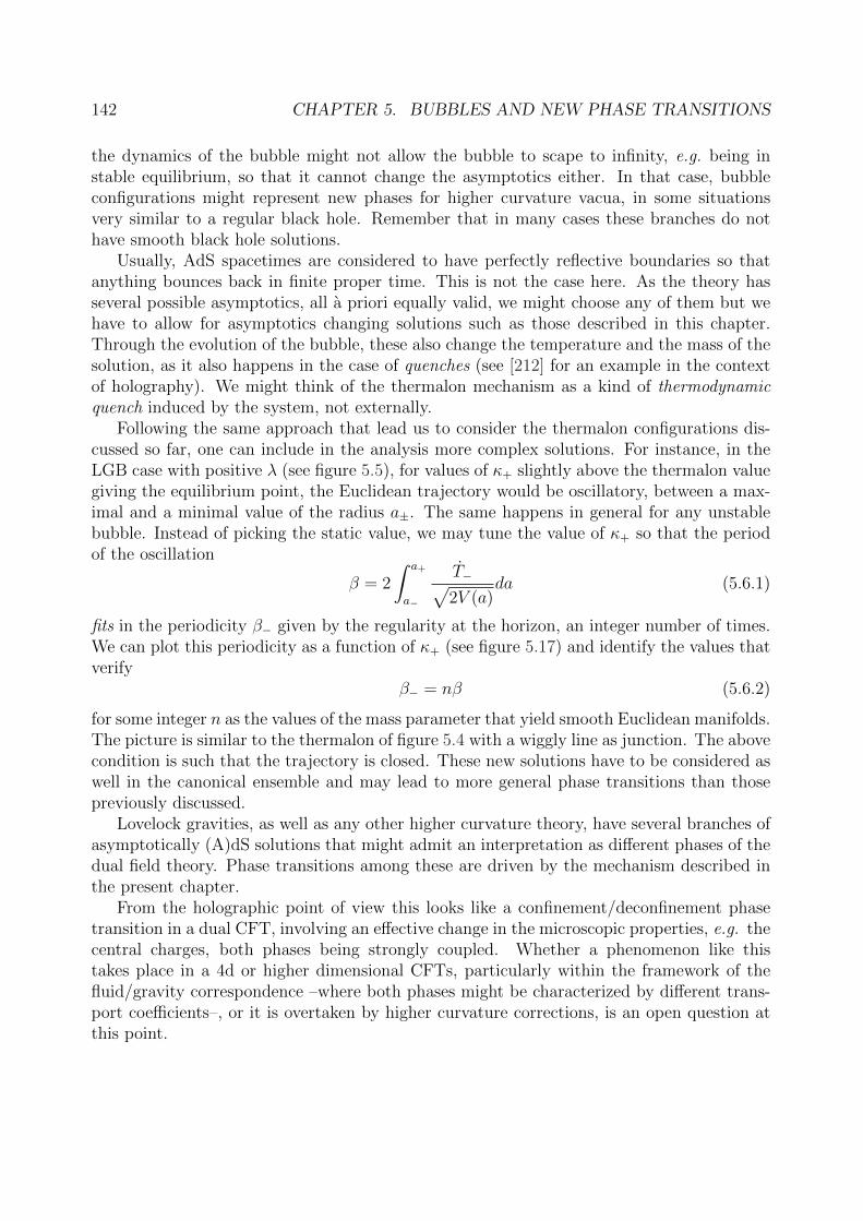
142 CHAPTER 5. BUBBLES AND NEW PHASE TRANSITIONS
the dynamics of the bubble might not allow the bubble to scape to infinity, e.g. being instable equilibrium, so that it cannot change the asymptotics either. In that case, bubbleconfigurations might represent new phases for higher curvature vacua, in some situationsvery similar to a regular black hole. Remember that in many cases these branches do nothave smooth black hole solutions.
Usually, AdS spacetimes are considered to have perfectly reflective boundaries so thatanything bounces back in finite proper time. This is not the case here. As the theory hasseveral possible asymptotics, all a priori equally valid, we might choose any of them but wehave to allow for asymptotics changing solutions such as those described in this chapter.Through the evolution of the bubble, these also change the temperature and the mass of thesolution, as it also happens in the case of quenches (see [212] for an example in the contextof holography). We might think of the thermalon mechanism as a kind of thermodynamicquench induced by the system, not externally.
Following the same approach that lead us to consider the thermalon configurations dis-cussed so far, one can include in the analysis more complex solutions. For instance, in theLGB case with positive λ (see figure 5.5), for values of κ+ slightly above the thermalon valuegiving the equilibrium point, the Euclidean trajectory would be oscillatory, between a max-imal and a minimal value of the radius a±. The same happens in general for any unstablebubble. Instead of picking the static value, we may tune the value of κ+ so that the periodof the oscillation
β = 2
∫ a+
a−
T−√2V (a)
da (5.6.1)
fits in the periodicity β− given by the regularity at the horizon, an integer number of times.We can plot this periodicity as a function of κ+ (see figure 5.17) and identify the values thatverify
β− = nβ (5.6.2)
for some integer n as the values of the mass parameter that yield smooth Euclidean manifolds.The picture is similar to the thermalon of figure 5.4 with a wiggly line as junction. The abovecondition is such that the trajectory is closed. These new solutions have to be considered aswell in the canonical ensemble and may lead to more general phase transitions than thosepreviously discussed.
Lovelock gravities, as well as any other higher curvature theory, have several branches ofasymptotically (A)dS solutions that might admit an interpretation as different phases of thedual field theory. Phase transitions among these are driven by the mechanism described inthe present chapter.
From the holographic point of view this looks like a confinement/deconfinement phasetransition in a dual CFT, involving an effective change in the microscopic properties, e.g. thecentral charges, both phases being strongly coupled. Whether a phenomenon like thistakes place in a 4d or higher dimensional CFTs, particularly within the framework of thefluid/gravity correspondence –where both phases might be characterized by different trans-port coefficients–, or it is overtaken by higher curvature corrections, is an open question atthis point.
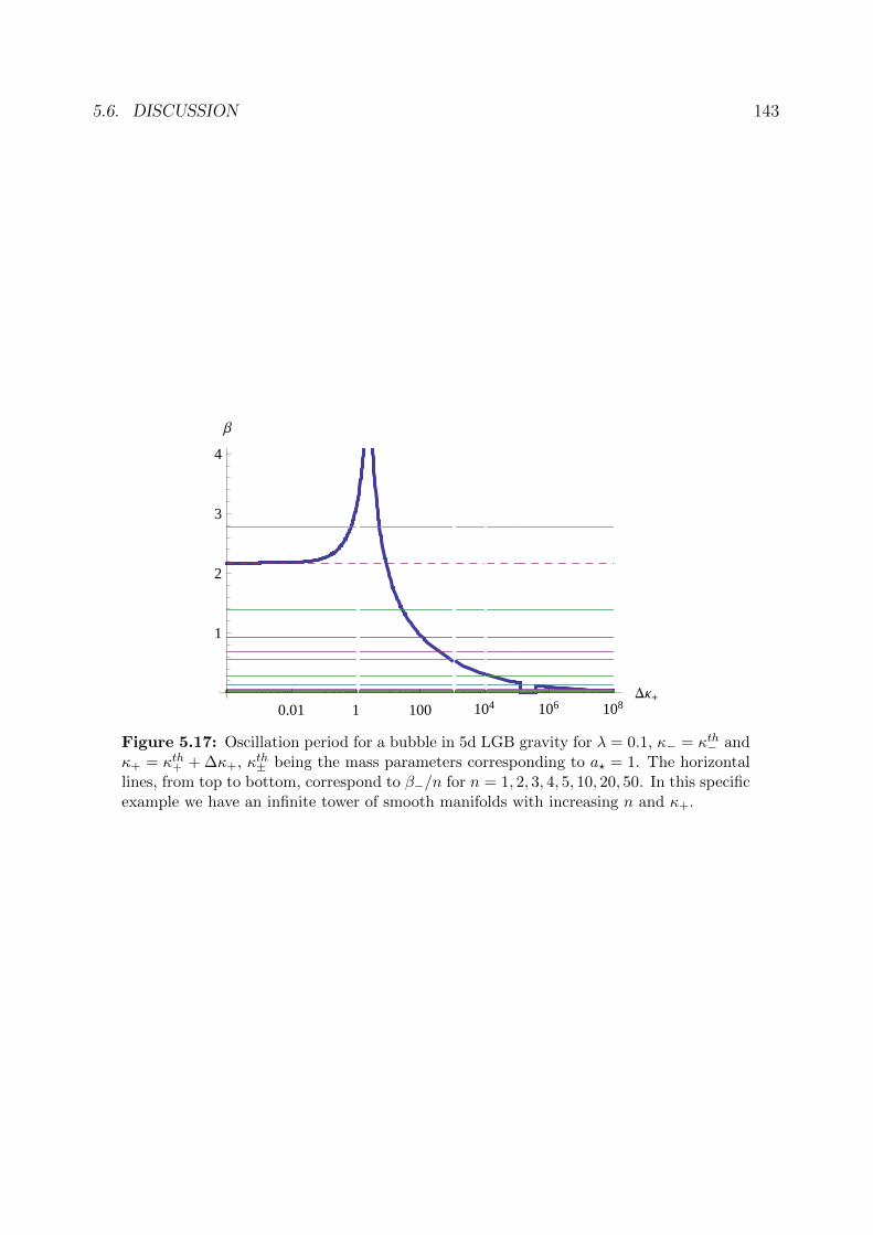
5.6. DISCUSSION 143
0.01 1 100 104 106 108DΚ+
1
2
3
4
Β
Figure 5.17: Oscillation period for a bubble in 5d LGB gravity for λ = 0.1, κ− = κth− andκ+ = κth+ + ∆κ+, κth± being the mass parameters corresponding to a? = 1. The horizontallines, from top to bottom, correspond to β−/n for n = 1, 2, 3, 4, 5, 10, 20, 50. In this specificexample we have an infinite tower of smooth manifolds with increasing n and κ+.

Part II
HIGHER CURVATURE GRAVITY& HOLOGRAPHY
145

Chapter 6
AdS/CFT and Lovelock gravity
“But although all our knowledge begins with experience,it does not follow that it arises from experience.”
Immanuel Kant
Near the end of the XIXth century, physics was thought to be an almost finished disci-pline. For the scientific community at the time, Newtonian mechanics on the one hand andMaxwell’s theory of electromagnetism on the other would describe perfectly any physicalprocess. They could not be more mistaken. During the last years of the century and the firstdecades of the next, some new experimental evidence would require a complete revision ofour scientific paradigm. This revolution is the origin of Einstein’s special theory of relativityand also of quantum mechanics. Moreover, the quest for reconciling the apparent inconsis-tencies between these two theories motivated the birth of quantum field theory (QFT), thebasis of our current understanding of particle physics.
Furthermore, Newtonian gravity was neither compatible with the new paradigm of specialrelativity, the solution of this problem being on the origin of Einstein’s formulation of generalrelativity. We already talked about general relativity and its higher curvature generalizationin the first part of this thesis. QFT and general relativity are the two pillars of contemporarytheoretical physics, key to our current knowledge of the Universe. Both theories have beensuccessfully tested to extremely high accuracy and are thought to faithfully describe anyphysical process within the corresponding regimes of applicability. The Higgs boson was theonly missing particle of the standard model of particle physics, the last discovered buildingblock of our understanding of the most fundamental aspects of the physical world. Is thisdescription of physics complete as our XIXth century fellows thought?
QFT ad general relativity are two conceptually very different theories and apply to almostcomplementary regimes. However, both theories are contradictory in situations for which
147
148 CHAPTER 6. ADS/CFT AND LOVELOCK GRAVITY
both gravitational and quantum mechanical effects are relevant. In other words, despite allits successes, general relativity, or any classical modification of it such as Lovelock theory,can not be a complete theory of gravity. In order to understand phenomena at energy scales
beyond the Planck mass, MPl =√
~cGN
(or distances smaller than the Planck length), a
full quantum theory of Gravity is needed. Moreover, the new theory must approach theprecedent theories in the respective regimes of validity, while solving their incompatibilities.The search for a viable theory of Quantum Gravity is one of the most important problemsof our time, where by viable we mean theoretically but also experimentally consistent withthe Universe we live in.
One of the key points of the disagreement between the two frameworks is the role playedby the spacetime on each of them. From the QFT point of view this four dimensionalmanifold is just a fixed background, the arena where all physical processes happen. Incontrast, from the GR perspective gravity is just another dynamical field and, as such, thereis no a priori reason for it not to be quantized. Nevertheless it cannot be quantized in thesame way as all the other fields. Einstein-Hilbert, or any other gravity action, describesthe dynamics of a spin two particle but renormalizability constrains the possible spin in thespectrum to be one or less. Moreover, the Weinberg-Witten theorem [213] also restricts thespin of particles if they are charged under Poincare covariant currents. Gauge bosons andgravitons scape the assumptions of the theorem because of gauge symmetry, but this alsoforces the spacetime to be dynamical. Furthermore, this result also forbids the existenceof composite gravitons (see [214] for a recent discussion on the topic). One cannot get amassless spin two bound state in a theory with a local stress-energy tensor, showing thatone cannot start with a local theory in Minkowksi space and generate Einstein gravity as anemergent phenomenon, thus eliminating the last possibility of consistently describe spin twoparticles in a fixed Minkowsky background.
One of the candidate quantum theory of gravity is string theory, even though it wasborn in a quite different context. In fact, it was first proposed in the sixties as a theory ofstrong interactions, mainly because of the way the meson spectrum is organized in Reggetrajectories. We now describe the strong interaction through Quantum Chromodynamics(QCD) although there is still much to be understood, mostly due to the fact that it isstrongly coupled at low energies. Most tools used in QFT are only suited for the peturbativeregime.
It was after the rise of QCD that it was recognized that the spectrum of closed stringtheories always includes a spin 2 massless excitation with the correct properties to describea graviton, the quantum of the gravitational interaction. String theory was the first consis-tent candidate for a complete quantum description of gravity. Its main advantage is thatsofter interactions between stringy objects would help bridle the divergences encountered inprevious quantization approaches using point-like gravitons.
The early connection to strong interactions was premonitory. As we will describe stringtheory has offered many new and deep perspectives into QFT and its connection to gravity.Gerard ’t Hooft was one of the scientists that most contributed to the understanding ofthat connection. Looking for new ways of simplifying computations in QCD, he consideredSU(N) instead SU(3) gauge theory with a very large number of colors, N [215]. Perhapsthe understanding of this simplified theory would shed some light on QCD or we can try
6.1. THE MALDACENA CONJECTURE 149
to approach the physical value N = 3 with a perturbative expansion in 1/N . Using hisfamous double line representation, ’t Hooft found that Feynman diagrams may be organizedin a double expansion in terms of the genus g of the two dimensional surface defined by thediagrams and the ’t Hooft coupling1 λ = g2
YMN as
∞∑g=0
(g2
YM
)2g−2∞∑h=2
Cg,hλh , (6.0.1)
strongly reminiscent of the perturbative expansion of string theory with string coupling
gs ∼ g2YM . (6.0.2)
The ’t Hooft limit corresponds to large N , N → ∞, keeping the ’t Hooft coupling λ fixed.In this regime, only planar (g = 0) Feynman diagrams contribute and the putative stringtheory becomes effectively free.
The other contribution of ’t Hooft, that of holography [216,217], is not less fundamentalfor the aim of the present essay. Motivated by the work of Bekenstein and Hawking on theentropy of black holes and its scaling with the area of the system, ’t Hooft and later Susskindproposed the holographic principle. According to this proposal, the maximum entropy in aspacetime volume is proportional to its surface area. This is far smaller than the entropyof any local QFT on the same space, even with some UV cut-off, as such a theory wouldhave an entropy which scales with the volume. Hence, for a string theory or any quantumtheory of gravity to be dual to a QFT, the field theory would have to be formulated on onelower dimension, so that the degrees of freedom can in principle be matched. The idea of thegravitational theory as effectively described in a lower dimensional space is also reinforcedby the fact that it cannot have local gauge invariant observables. The notion of localityis tightly tied to the notion of coordinate frame and in a diffeomorphism invariant theorylocal quantities are thus not gauge invariant, observables having to lie at the boundary ofthe spacetime. One example of this is the gravitational energy not being localized anywherein spacetime. Just the total mass, integrated over the spacetime hence not dependent onpositions, is a well-defined gauge invariant observable.
6.1 The Maldacena conjecture
The Weinberg-Witten theorem effectively forbids the notion of a spin two particle in a localQFT with Poincare invariance. However the holographic principle readily offers an elegantway out that immediately solves some of the apparent inconsistencies. The graviton doesnot appear in the QFT but it has to live in a higher dimensional spacetime.
As it has been argued, the large N limit of SU(N) gauge theories is expected to bedescribed in terms of strings. Naively, for d = 4 Yang Mills theory one would expect to geta bosonic string theory in four dimensions. However, the bosonic string is not consistent
1Even though we use the same symbol λ for the ’t Hooft and the LGB couplings, it will be easy to knowwhich one we are referring to as they never appear in the same context.
150 CHAPTER 6. ADS/CFT AND LOVELOCK GRAVITY
quantum mechanically in d = 4 and this is not correct. The reason for this inconsistency isthat the classical Polyakov action,
I ∼∫dDx√−ggαβ∂αX∂βX , (6.1.1)
has a Weyl symmetry gαβ → Ωgαβ which is not a symmetry quantum mechanically, it hasan anomaly. In the quantum theory, under a change of the metric of the form gαβ = eφgαβthe partition function,
e−Ieff =
∫D[X]D[b, c]e−I[X,g]−I[b,c,g] , (6.1.2)
changes as [218]
Ieff(g)− Ieff(g) =26−D
48π
∫dDx√−g(
1
2(∇φ)2 + R(2)φ+ µ2eφ
), (6.1.3)
where R(2) is the Ricci scalar on the worldsheet of the string.This action for φ is called Liouville action. Even though the initial classical action for
the conformal factor in the metric was zero, a non-trivial action was generated quantummechanically. This new dynamic field can be thought of as an extra dimension of spacetimein the context of string theory. Being interested in gauge theories in four dimensions, wethen need to look for five dimensional strings. We need to specify the space where thesestrings move. It should have four dimensional Poincare symmetry, so the metric has theform
ds2 = ω2(z)(ds21+3 + dz2) , (6.1.4)
where we have used the reparametrization invariance to set the coefficient of dz2 equal tothat of the 4 dimensional metric.
Consider now a conformal field theory, e.g. N = 4 Super Yang Mills. In this case theaction is also invariant under conformal coordinate transformations such that g = Ω2(x)g,and Ω is any function. Then, a scale transformation x→ λx should be a symmetry. However,string theory has a scale, the string length ls. Then, the only way that our string theorycould be symmetric under the scale transformation is that this corresponds to an isometry ofthe background. This implies that the extra dimension must also change under this scaling,z → λz and that the form of the warp factor is ω(z) = b/z. So we end up dealing with 5dimensional anti-de Sitter space
ds2 =b2
z2(dx2
1+3 + dz2). (6.1.5)
In 1997 Maldacena [30] provided a precise realization of the duality between gauge the-ory and gravity, allowing for a detailed understanding of the facts examined above. Thiswork, together with [219] and [136] where a precise dictionary between these naively very dis-parate theories was constructed, laid the foundations of what later became the gauge/gravityduality, or AdS/CFT in its most popular incarnation (see also [220]).
6.1. THE MALDACENA CONJECTURE 151
The AdS/CFT correspondence is a relation between a conformal field theory (CFT) ind dimensions and a gravity theory in (d + 1)-dimensional anti-de Sitter background. Thefirst hint of this duality is the degree of symmetry in both sides of the correspondence. Thegroup of isometries of AdSd+1 space is SO(2, d), which coincides with the conformal group ind dimensions. In fact it can be shown that the group of isometries of AdS space acts on itsboundary as the conformal group acting on Minkowski space. This is one of the reasons whythe CFT is usually said to live on the boundary of AdS. The extra dimension is related tothe energy scale in such a way that it is sometimes said that the AdS/CFT correspondencegeometrizes the renormalization group flow of the QFT.
In the context of string theory, gauge theories describe the low energy dynamics of openstrings living on several superposed D-branes. For example, the field theory on N D3-branesis 4d N = 4 U(N) Yang Mills at low energies. These open string have the possibility ofcolliding and merging to form a closed string, not bound to the brane any more. The bulkspacetime where this closed strings move is warped due to the presence of the D-branes. Infact, as Polchinski proved [221], D-branes are actually the same object as p-branes, whichare solutions of IIB supergravity in ten dimensions. The metric for one of this solutionsextended in three spatial dimensions is
ds2 = H−1/2(r)(−dt2 + d~x23 +H1/2(r)(dr2 + r2dΩ2
5) , (6.1.6)
where H = 1 + b4/r4 and b4 = 4πgsNl4s . The directions d~x3 are those parallel to the brane,
and r is the distance from the brane. From the point of view of a distant observer, anyexcitation near the brane (the horizon, r = 0) has very small energy,
E∞(r) =√−g00Er ∼ rEr → 0 . (6.1.7)
.Then, we conclude that at low energies only these excitations will survive. The near
horizon geometry, r → 0 due to the D3-branes is
ds2 ≈ b2
z2(−dt2 + d~x2
3 + dz2) + b2dΩ25 , (6.1.8)
where we have defined z = b2/r. This is the metric of AdS5 × S5, both factor spaces havingthe same radius b. The low energy dynamics of closed strings is determined by the usualaction of general relativity (with some extra fields), then, we have gravity in an AdS5 × S5
background at low energies. The AdS/CFT correspondence conjectures that, in the lowenergy regime, the two alternative descriptions should be equivalent. So N = 4 U(N) YangMills is equivalent to gravity in AdS5 × S5 [222]. This relation can be understood as anexample of the open-close string duality. In this context, gravity (or more precisely type IIBsupergravity) is the low energy limit of (type IIB) superstring theory, which is consistent inten dimensions.
Since the gauge theory describes the dynamics of open strings whereas gravity describesclosed strings moving in the bulk, we can identify in the usual stringy way
g2YM = 4πgs , (6.1.9)
152 CHAPTER 6. ADS/CFT AND LOVELOCK GRAVITY
in agreement with the generic expectations of ’t Hooft’s 1/N expansion. Beyond that leadingSUGRA approximation, gs and α′ correspond to 1/N and 1/λ corrections respectively.
The relation between the two theories is a duality. The gravity description is a goodapproximation to string theory if the radius of the space is much larger than ls, since ls isthe intrinsic size of the graviton. The radius of AdS space (6.1.6) is related to the ’t Hooftcoupling such that this implies
b
ls∼ λ1/4 1 (6.1.10)
We also require that string corrections are small so gs → 0, thus we need to consider thelarge N limit of the theory.
In the field theory side, the large N theory has effective coupling λ = g2YMN such that
when this coupling is small, λ 1, we have a well-defined perturbative field theory, whereasin the opposite strongly coupled regime (the ’t Hooft limit) of the gauge theory we expectstrings. This is the same regime for which the classical gravitational description is valid.
Then, in the region where the ’t Hooft coupling is very small, λ 1, the gauge theorydescription is weakly coupled and the other (gravity) is strongly coupled. The opposite istrue when this parameter is large. This is what makes the conjecture so interesting but alsoso hard prove or refute. In the specific example being discussed here, supersymmetry ensuresthat there are some quantities that are independent of the coupling. Computing these onboth sides, and checking that they agree, we have checks of the duality [222]. Some of themost convincing tests have been recently reviewed in [223].
The AdS/CFT correspondence is by now a well-established non-perturbative duality ofparamount importance. After several years of research, it has overpassed dozens of checksand has been applied in a plethora of systems that go far beyond the large N limit of N = 4super Yang-Mills theory in four dimensions, originally portrayed by Maldacena [30]. Thestrongest version of the conjecture is that this correspondence is valid for any value of gsand N , even if we are only able to make calculations in certain limits. In fact, there havebeen found many non-trivial examples of finite N and λ corrections that agree between AdSand CFT theories. The pursuit of a interpolation between the respective regimes where thestring or gauge theory descriptions are reliable has delivered many insightful developmentsand ideas, e.g. integrability of planar N = 4 SYM (see [224] for a review) and also recentlythe recovery of the bootstrap program for CFTs [225].
The correspondence has also been generalized to a plethora of other examples, distilled ina similar manner from other brane configurations in string theory. The known dual couplesare impressively varied, with different dimensionality, global and gauge symmetries or particlecontent. However, the relevant closed string or (super)gravity theory dual to physical QCDremains elusive. The advent of the gauge/gravity correspondence has motivated importantachievements not only for QFT and gravity but also in mathematics and in other seeminglyunrelated branches of physics, from Condensed Matter to hydrodynamics.
6.1.1 Correlation functions
The dynamics of any CFT is defined by the correlation functions of the gauge invariantlocal operators in its spectrum. The dynamical information of AdS/CFT duality can then
6.1. THE MALDACENA CONJECTURE 153
be realized as a relation between the generating functional for CFT correlators and thestring theory partition function with appropriate boundary conditions on the AdS boundary[136,226]. In the case of a scalar field, φ(z,x) , we have⟨
exp
(i
∫Σ
dxµφ0(x)O(x)
)⟩CFT
= Zstring[φ(0,x) = φ0(x)] , (6.1.11)
where the asymptotic value (or boundary condition) of the scalar field in AdS acts as asource for the dual CFT scalar operator O. Moreover, the hamiltonian is realized in theCFT as the dilatation operator in such a way that energy in AdS corresponds to conformaldimension in the field theory, these being related as
m2 = ∆(∆− d) . (6.1.12)
The same can be also generalized to operators with spin. In the CFT side the spectrumwill always contain many operators with different spins and conformal dimension. One ofthem is universal in the sense that it is present for any CFT and that it has some veryspecific properties. This operator is the stress-energy tensor and it is realized in the dualgravitational picture by the graviton. Restricting to purely gravitational theories will thenamount to the analysis of correlators of the stress-energy tensor2. In that case we cancompute the generating function as⟨
exp
(∫dx ηab(x) Tab(x)
)⟩CFT
= Z [gµν ] ≈ exp(−I[gµν ]
), (6.1.13)
where Z [gµν ] is the partition function of quantum gravity –the same we used to discussthermodynamic properties of black holes– and gµν = gµν(z,x) such that gab(0,x) = ηab(x).From this expression, correlators of the stress-energy tensor can be obtained by performingfunctional derivatives of the gravity action with respect to the boundary metric. This, inturn, is simply given by considering gravitational fluctuations around an asymptotically AdSconfiguration of the theory. The bulk metric acts as a source for the stress-energy tensor inthe boundary (and viceversa).
6.1.2 Confinement/deconfinement phase transition
The gravity (or string theory) partition function is in general computed by integrating overbulk metrics, g, that induce a given metric h on the boundary. This is calculated in thesame way we described at the end of section 3.1, in the framework of Euclidean QuantumGravity. Again, in the stationary phase approximation, one can compute Z(h) by findinga solution g for the Einstein equations with the required boundary behavior, and setting
Z(h) ≈ exp(−I[g]
). If there are several solutions which are asymptotic to the given
boundary, the leading contribution comes from the solution with the lowest action andwe have phase transitions when other solution dominates over the previous one. The only
2§ This truncation, to pure gravity in the bulk, is not always self-consistent, as demonstrated for instancein [10]
154 CHAPTER 6. ADS/CFT AND LOVELOCK GRAVITY
difference with the Euclidean Quantum Gravity case is that here we have to consider solutionsof AdS5×S5, not just AdS5. In Einstein’s theory, any asymptotically AdS5 solution with anextra S5 factor is a consistent solution for the corresponding field equations in ten dimensions.In the higher curvature case this is not as simple.
We consider N = 4 Super Yang Mills theory at finite temperature on a spatial manifoldS3 or R3. We must compute the partition function on S1×S3 with respective radius β and b.By conformal invariance only the ratio β/b matters. This can be regarded as a dimensionlesstemperature on the CFT side, TCFT = b/β = bT .
It has been shown (see citation in [137]) that the N = 4 theory on S1 × S3 has a phasetransition as a function of β/b in the planar limit. The large β/b phase has some propertiesin common with the usual large β (small T ) phase of confining gauge theories, while thesmall β/b phase is analogous to a deconfining phase. In the large N limit, a criterion forconfinement is whether the free energy (after subtracting a constant from the ground stateenergy) is of order one, reflecting the contributions of singlet color hadrons, or of order N2,reflecting the contributions of gluons [137].
We can compute the partition function of this theory from the gravity side using thecorrespondence. In the case of Einstein-Hilbert gravity in five dimensions, considering theextra V ol(S5) ∼ b5 factor arising from the volume of the 5-sphere, for the solution containinga black hole we find F/T ∼ b8 ∼ N2 as expected for a deconfining phase. In contrast, thelow temperature phase we have a trivial N2 contribution coming from the spacetime volume.The excitations (just thermal radiation) have no dependence on N and give a contributionof order one, as in a confining phase.
Thus, the Hawking-Page phase transition we found in the analysis of the canonical ensem-ble of AdS space corresponds to a confinement/deconfinement phase transition in the N = 4Super Yang Mills theory living on its boundary, for Einstein-Hilbert gravity and, by analogy,also for Lovelock theories in AdS. For non-conformal theories, such as that described by theKlebanov-Strassler model [227], the confinement/deconfinement transition occurs at finitetemperature also in R3. In that context the associated QGP might be affected by hydro-dynamic effects that may dynamically shift the temperature at which the phase transitionoccurs [7]. The viscous terms in a relativistic fluid result in reducing the effective pressure,thus facilitating the nucleation of bubbles of a stable phase. This is known as cavitation.The effect is particularly pronounced in the vicinity of (weak) first-order phase transitions.We can use the holographic correspondence to study cavitation in strongly coupled non-conformal plasmas close to their confinement phase transition. An example is presented inAnnex D for the case of planar cascading gauge theory. While in this particular model theshift of the deconfinement temperature due to cavitation does not exceed 5%, we speculatethat cavitation might be important near the QCD critical point.
6.1.3 Effective conformal theories and local AdS dynamics
We can take an alternative point of view on the AdS/CFT correspondence and use the aboveprescription in order to effectively define and study CFTs in higher dimensions. We just needto write down a gravitational action with any number of matter fields. The AdS partitionfunction will then provide correlation functions for the dual operators that automatically
6.1. THE MALDACENA CONJECTURE 155
satisfy conformal symmetry. These will however be subject to other physical constraintssuch as unitarity, causality, crossing, etc. in such a way that these translate into constraintson the spectrum and possible interaction terms. This effective conformal theory (see [228]and references therein) would describe the low-lying spectrum of the dilatation operator ina CFT, equivalent to low energy spectrum in AdS. Such an effective theory is useful whenthe spectrum contains a hierarchy in the dimension of operators, in such a way that wecan perform an expansion for large gap. These criteria ensure that there is a regime wherethe dilatation operator is modified perturbatively. Local interactions in AdS thus provide avery efficient way of organizing perturbations of the dilatation operator respecting conformalinvariance, much as Minkowski space naturally describes Lorentz invariant perturbations ofa QFT hamiltonian. This approach might also be useful to understand which CFTs have awell-behaved AdS description.
This perspective may also provide some interesting insights into higher dimensional CFTs.It is indeed unclear whether there are non-trivial higher dimensional CFTs. In generalit is thought that interacting CFTs do not exist in dimensions higher than six. Due todimensionality any interaction term is irrelevant so that there is no obvious way to defineinteracting CFTs. There seems to be an avenue for their formulation in terms of p-formswith p ≥ 2 (so-called generalized gerbe theories) [35]. Also from the bootstrap perspective,it is not at all obvious that there is no solution. It would be good to understand this betterand the study of gravity in AdS opens an interesting window that might shed some light onthe issue.
In the remaining chapters of this thesis, we will investigate the uses of the frameworkof the gauge/gravity duality in the case of Lovelock theories and extract some of its con-sequences. This provides interesting information both from a fundamental as well as froma more effective perspective. Higher-curvature corrections to the Einstein-Hilbert actionappear as next to leading orders in the low-energy expansion of string theory, e.g. theLanczos-Gauss-Bonnet term [29], being in any case perturvative. In the context of hologra-phy, generic higher curvature terms may correspond both to finite N or λ corrections. Seefor instance [229, 230] for a recent discussion regarding the LGB term. Even if, in the caseof LGB gravity, its stringy origin allows for establishing a detailed holographic dictionary,this does not happen for higher order Lovelock theories. Still Lovelock gravity in sevendimensions might help to understand the role of cubic terms in the duality and provide in-formation about more general six dimensional CFTs. In turn higher order Lovelock terms,may help understand the elusive higher dimensional CFTs, although there is no explicitstring construction for them, neither for AdS spaces in dimension higher than seven. Thesetheories constitute perfect toy models to test our ideas about the holographic duality withthe addition of finite higher curvature corrections. These introduce some of the characteristicfeatures of higher curvature gravities, such as several branches, new types of singularitiesand more complex dynamics, without problematic higher derivative degrees of freedom.
From the CFT point of view, any stringy realization of the gauge/gravity duality willyield correlation functions for the stress-energy tensor analogous to those arising for Einstein-Hilbert gravity, with the possibility of some small correction due to higher order terms.The analysis of the Lovelock family will in turn allow for the exploration of much moregeneral CFTs of arbitrary dimensionality and beyond the perturbative regime. All results
156 CHAPTER 6. ADS/CFT AND LOVELOCK GRAVITY
are consistent and compelling enough to pursue our investigations.
6.2 Lovelock theories and holography
Lovelock theory has a rich structure of AdS vacua. Correspondingly, the AdS/CFT cor-respondence tells us that there should be an analogously complex structure of dual CFTs.We know very little about these higher-dimensional CFTs. Indeed, at least for the caseof supersymmetric CFTs, one naively expects to have at most six dimensional non-trivialunitary conformal field theories, based on the algebraic construction by Nahm [231]. Forhigher-dimensional CFTs, the general expectation is that they are not Lagrangian theoriesand their constituent degrees of freedom are not gauge fields but possibly self-dual p-forms(in the case of even spacetime dimensions) [35]. These theories should have a stress tensorand conformal symmetry will constrain their 2- and 3-point functions as we shall presentlydescribe.
6.2.1 CFT unitarity and 2-point functions
Consider a CFTd−1. The leading singularity of the 2-point function in any number of di-mensions is fully characterized by the central charge CT [232]
〈Tab(x)Tcd(0)〉 =CT
x2(d−1)Iab,cd(x) , (6.2.1)
where
Iab,cd(x) =1
2
(Iac(x) Ibd(x) + Iad(x) Ibc(x)− 1
d− 1ηab ηcd
), (6.2.2)
whereas Iab(x) = ηab − 2xa xb/x2. This structure is completely dictated by conformal sym-
metry. For instance, CT is proportional in a CFT4 to the standard central charge c thatmultiplies the (Weyl)2 term in the trace anomaly, CT = 40 c/π4.
The holographic computation of CT was performed in [37] for LGB in various dimensionsand in [3] for Lovelock theory. Since CT appears in the general 2-point function of the stresstensor, it is sufficient to consider a particular set of components. Following [37] we considerthe correlator 〈Txy(x)Txy(0)〉. According to the AdS/CFT dictionary, it is sufficient to takea metric fluctuation hxy(z,x) = L2/z2 φ(z,x) about empty AdS with cosmological constantΛ?. Expanding the Lovelock action to quadratic order in φ, and evaluating it on-shell,
Iquad =Υ′[Λ?]
2(−Λ?)d/2
∫dx z2−d (φ ∂zφ) . (6.2.3)
Imposing the boundary conditions φ(0,x) = φ(x), the full bulk solution reads
φ(z,x) =d
d− 2
Γ[d]
πd−1
2 Γ[d−1
2
] ∫ dyzd−1
(z2 + |x− y|2)d−1Iab,cd(x− y) φ(y) . (6.2.4)
6.2. LOVELOCK THEORIES AND HOLOGRAPHY 157
Plugging this expression into Iquad, we obtain
Iquad =CT2
∫dx
∫dy
φ(x) Iab,cd(x− y) φ(y)
|x− y|2(d−1), (6.2.5)
where CT is the central charge of the dual CFTd−1,
CT =d
d− 2
Γ[d]
πd−1
2 Γ[d−1
2
] Υ′[Λ?]
(−Λ?)d/2. (6.2.6)
It is easy to see that this had to be the result as the computation basically correspondsto that of Einstein-Hilbert gravity with the overall constant Υ′[Λ?]. The upshot of thiscomputation in an AdS vacuum, Λ? < 0, is thought-provoking:
CT > 0 ⇐⇒ Υ′[Λ?] > 0 . (6.2.7)
The latter inequality, in the gravity side, corresponded to the generalized BD conditionpreventing ghost gravitons in the branch corresponding to the AdS vacuum with cosmologicalconstant Λ?. Thereby, unitarity of the CFT and the absence of ghosts gravitons in AdS,seem to be the two faces of the same holographic coin. The positivity of Υ′[Λ] has beenproven to be true for the EH branch of solutions in any Lovelock theory [2]. Thus, thisbranch is protected from BD instabilities and the corresponding dual theory is unitary.
6.2.2 3-point function and conformal collider physics
The form of the 3-point function of the stress-tensor in a (d− 1)-dimensional conformal fieldtheory is highly constrained. In [232,233], it was shown that it can always be written in theform
〈Tab(x)Tcd(y)Tef (z)〉 =
(AI(1)
ab,cd,ef + B I(2)ab,cd,ef + C I(3)
ab,cd,ef
)(|x− y| |y − z| |z− x|)d−1
(6.2.8)
where the form of the tensor structures I(i)ab,cd,ef will be irrelevant for us here. Energy con-
servation also implies a relation between the central charge CT appearing in the 2-pointfunction, and the parameters A,B, C, namely
CT =πd−1
2
Γ[d−1
2
] (d− 2)(d+ 1)A− 2B − 4d C(d− 1)(d+ 1)
. (6.2.9)
Since we have already computed CT in the previous section, we are left with two independentparameters to be calculated.
A convenient parametrization of the 3-point function of the stress-tensor was introducedin [234]. Consider a gedanken collision experiment in an arbitrary CFTd that mimics theframework developed in [235,236] for e+–e− annihilation in QCD. We would like to measurethe total energy flux per unit angle deposited in calorimeters distributed around the collisionregion,
E(n) = limr→∞
rd−3
∫ ∞−∞
dt ni T 0i(t, r n) , (6.2.10)
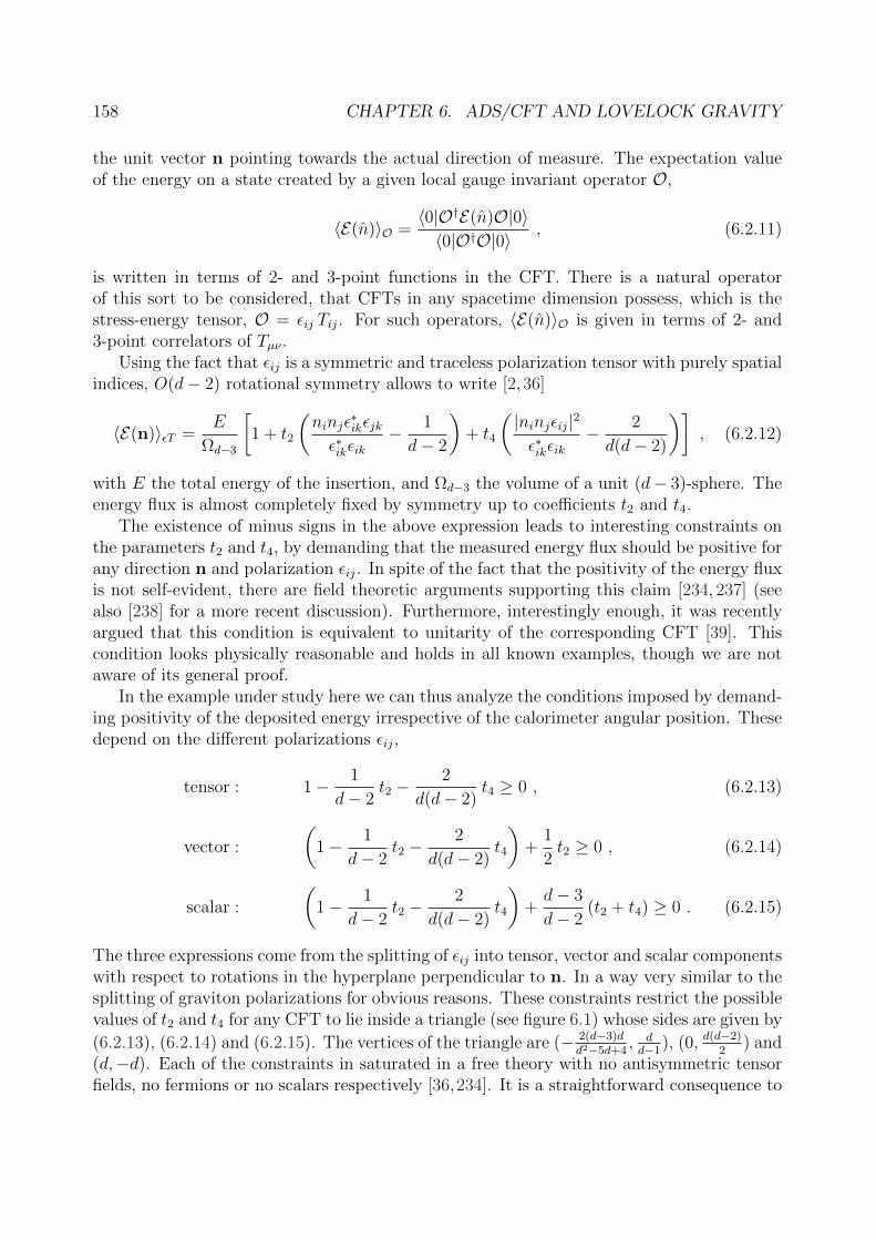
158 CHAPTER 6. ADS/CFT AND LOVELOCK GRAVITY
the unit vector n pointing towards the actual direction of measure. The expectation valueof the energy on a state created by a given local gauge invariant operator O,
〈E(n)〉O =〈0|O†E(n)O|0〉〈0|O†O|0〉
, (6.2.11)
is written in terms of 2- and 3-point functions in the CFT. There is a natural operatorof this sort to be considered, that CFTs in any spacetime dimension possess, which is thestress-energy tensor, O = εij Tij. For such operators, 〈E(n)〉O is given in terms of 2- and3-point correlators of Tµν .
Using the fact that εij is a symmetric and traceless polarization tensor with purely spatialindices, O(d− 2) rotational symmetry allows to write [2, 36]
〈E(n)〉εT =E
Ωd−3
[1 + t2
(ninjε
∗ikεjk
ε∗ikεik− 1
d− 2
)+ t4
(|ninjεij|2
ε∗ikεik− 2
d(d− 2)
)], (6.2.12)
with E the total energy of the insertion, and Ωd−3 the volume of a unit (d− 3)-sphere. Theenergy flux is almost completely fixed by symmetry up to coefficients t2 and t4.
The existence of minus signs in the above expression leads to interesting constraints onthe parameters t2 and t4, by demanding that the measured energy flux should be positive forany direction n and polarization εij. In spite of the fact that the positivity of the energy fluxis not self-evident, there are field theoretic arguments supporting this claim [234, 237] (seealso [238] for a more recent discussion). Furthermore, interestingly enough, it was recentlyargued that this condition is equivalent to unitarity of the corresponding CFT [39]. Thiscondition looks physically reasonable and holds in all known examples, though we are notaware of its general proof.
In the example under study here we can thus analyze the conditions imposed by demand-ing positivity of the deposited energy irrespective of the calorimeter angular position. Thesedepend on the different polarizations εij,
tensor : 1− 1
d− 2t2 −
2
d(d− 2)t4 ≥ 0 , (6.2.13)
vector :
(1− 1
d− 2t2 −
2
d(d− 2)t4
)+
1
2t2 ≥ 0 , (6.2.14)
scalar :
(1− 1
d− 2t2 −
2
d(d− 2)t4
)+d− 3
d− 2(t2 + t4) ≥ 0 . (6.2.15)
The three expressions come from the splitting of εij into tensor, vector and scalar componentswith respect to rotations in the hyperplane perpendicular to n. In a way very similar to thesplitting of graviton polarizations for obvious reasons. These constraints restrict the possiblevalues of t2 and t4 for any CFT to lie inside a triangle (see figure 6.1) whose sides are given by
(6.2.13), (6.2.14) and (6.2.15). The vertices of the triangle are (− 2(d−3)dd2−5d+4
, dd−1
), (0, d(d−2)2
) and(d,−d). Each of the constraints in saturated in a free theory with no antisymmetric tensorfields, no fermions or no scalars respectively [36,234]. It is a straightforward consequence to
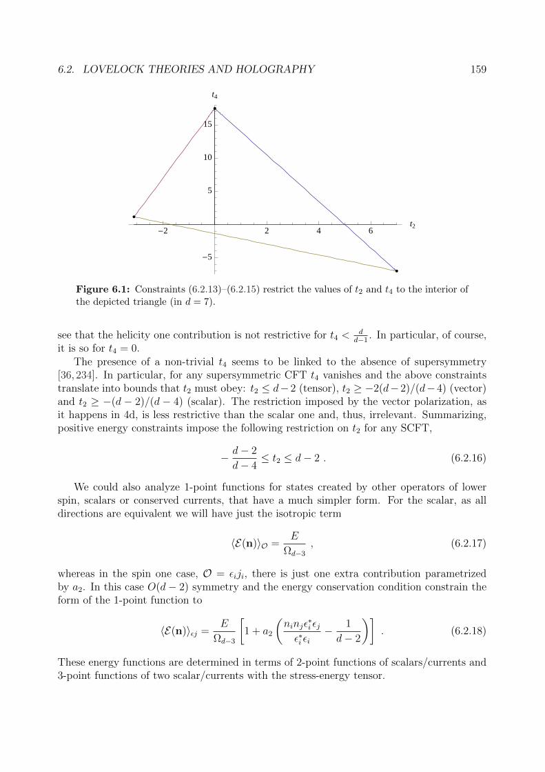
6.2. LOVELOCK THEORIES AND HOLOGRAPHY 159
-2 2 4 6t2
-5
5
10
15
t4
Figure 6.1: Constraints (6.2.13)–(6.2.15) restrict the values of t2 and t4 to the interior ofthe depicted triangle (in d = 7).
see that the helicity one contribution is not restrictive for t4 <dd−1
. In particular, of course,it is so for t4 = 0.
The presence of a non-trivial t4 seems to be linked to the absence of supersymmetry[36, 234]. In particular, for any supersymmetric CFT t4 vanishes and the above constraintstranslate into bounds that t2 must obey: t2 ≤ d− 2 (tensor), t2 ≥ −2(d− 2)/(d− 4) (vector)and t2 ≥ −(d − 2)/(d − 4) (scalar). The restriction imposed by the vector polarization, asit happens in 4d, is less restrictive than the scalar one and, thus, irrelevant. Summarizing,positive energy constraints impose the following restriction on t2 for any SCFT,
− d− 2
d− 4≤ t2 ≤ d− 2 . (6.2.16)
We could also analyze 1-point functions for states created by other operators of lowerspin, scalars or conserved currents, that have a much simpler form. For the scalar, as alldirections are equivalent we will have just the isotropic term
〈E(n)〉O =E
Ωd−3
, (6.2.17)
whereas in the spin one case, O = εiji, there is just one extra contribution parametrizedby a2. In this case O(d− 2) symmetry and the energy conservation condition constrain theform of the 1-point function to
〈E(n)〉εj =E
Ωd−3
[1 + a2
(ninjε
∗i εj
ε∗i εi− 1
d− 2
)]. (6.2.18)
These energy functions are determined in terms of 2-point functions of scalars/currents and3-point functions of two scalar/currents with the stress-energy tensor.
160 CHAPTER 6. ADS/CFT AND LOVELOCK GRAVITY
For conformal field theories with a weakly curved gravitational dual, it is possible to com-pute t2 and t4 holographically. Also a2 if we include a vector field, otherwise this coefficientis trivially zero. This was first done in detail for LGB theory in various dimensions [37] andlater applied to quasi-topological gravity in [71]. The calculation proceeds by consideringthe vacuum AdS solution perturbed by a shock wave, which corresponds holographically toa T−− insertion. By adding a transverse metric fluctuation, one reads off the interactionvertex from the action, and from that one obtains t2 and t4.
Shock wave backgrounds were also considered by Hofman [237] in the context of five-dimensional LGB theory and was to arbitrary higher-dimensions in [1] There it was foundthat in the presence of the shock wave there is the possibility for causality violation in thedual field theory. This places bounds on the parameters of the theory, which precisely matchthose portrayed in (6.2.13 - 6.2.15). This will be the focus of the next chapter.
We would now like to generalize this story to higher Lovelock theories. We consider,along the lines of [1], a helicity two perturbation φ(u, v, r) in the shock wave background
ds2AdS,sw =
N2# L
2
z2
(−du dv + dxi dxi + 2 ε φ dx2 dx3 + dz2
)+ f(u)$(xa, z) du2 , (6.2.19)
where z = L2/r is the Poincare coordinate and u, v = x0 ± xd−1 are light-cone coordinates.This amounts to choosing just one non-vanishing component of the polarization tensor,ε23 6= 0. Leading contributions (in the high momentum limit) to the equations of motioncome from the exterior derivative of the perturbation of the spin connection.3 We get,
d(δω02) ≈ ε z2
L2N2#
[∂2vφ e
1 ∧ e2 +
(∂u∂vφ+
z2
L2N2#
f(u)$(xa, z) ∂2vφ
)e0 ∧ e2
],
d(δω12) ≈ ε z2
L2N2#
[(∂u∂vφ+
z2
L2N2#
f(u)$(xa, z) ∂2vφ
)e1 ∧ e2 + (· · · ) e0 ∧ e2
],
the ellipsis being used in the second expression since the corresponding term does not con-tribute to the equations of motion. The components with index 3 instead of 2 are the onlyremaining non-vanishing ones, and they are obtained just by changing4 φ→ −φ. The otheringredient we need is the curvature 2-form of the background metric, that can be written as
Rab = Λ(ea ∧ eb + f(u)Xab) , (6.2.20)
where Λ = − 1L2N2
#and Xab is an antisymmetric 2-form accounting for the contribution of
the shock wave. The relevant component here is
X1a =z2
L2N2#
[(2$ + z∂z$ − z2∂2
a$)e0 ∧ ea + (· · · ) e0 ∧ ez + (· · · ) e0 ∧ eb
],
X1(d−1) = −(
z
LN#
)2 [(3z∂z$ + z2∂2
z$) e0 ∧ ed−1 + (· · · ) e0 ∧ ea],
3The 3-point function will be determined by these kinds of terms; actually, terms in ∂2vφ since the vertexhas to be of the form φ∂2vφ∂i∂j$, as $ ∼ huu.
4dx2 → −dx3, dx3 → dx2, φ→ −φ is a symmetry of the background as well as of the vielbein basis.
6.2. LOVELOCK THEORIES AND HOLOGRAPHY 161
with a, b 6= 0, 1, d− 1, and b 6= a. The relevant equation of motion is given by δE3 ∧ e3 = 0,where
δE3 ∧ e3 =K∑k=1
k ak ε3f1···fd−1d(δωf1f2) ∧Rf3···f2k ∧ ef2k+1··· fd−1 3
= 4(−1)d−1 ε z2
L2N2#
K∑k=1
k ak Λk−1
[(d− 3)!
(∂u∂vφ+
z2
L2N2#
f(u)$∂2vφ
)
− (k − 1)(d− 5)!z2
L2N2#
f(u)(−4$ − 2z∂z$ + z2(∂2
2$ + ∂23$)
)∂2vφ
]. (6.2.21)
We made use of the equation of motion for the shock wave profile
2(d− 3)$ + (d− 6)z∂z$ − z2(∂a∂a$ + ∂2
z$) = 0 , a = 2, . . . d− 2 . (6.2.22)
This equation admits several solutions of the type
$ = α0zα
(z2 + (x2 − x20)2 + · · ·+ (xn − xn0 ))
β, (6.2.23)
where n is the number of transverse coordinates. The relevant solution for our discussion hereis the one given by α = d− 3 and β = d− 2. This shock wave profile has been argued [234]
to be the dual field configuration to E(n) provided xi0 = ni
1+nd−2 and f(u) = δ(u).
From (6.2.21), we shall focus on those terms proportional to ∂2vφ. The shock wave inter-
action term thus gives the following contribution to the equations of motion,[Υ′[Λ]$ +
Λ Υ′′[Λ]
(d− 3)(d− 4)
(4$ + 2z∂z$ − z2(∂2
2$ + ∂23$)
)]∂2vφ . (6.2.24)
There are extra non vanishing components of the form
δEi ∧ e2 ∼ ∂3∂i$∂2vφ ,
δEd−1 ∧ e2 ∼ 1
xd−1
(∂3$ + xd−1∂3∂d−1$
)∂2vφ ,
δEi 6=2,3 ∧ ej 6=2,3 ∼ ∂2∂3$∂2vφδ
ji .
However, these are irrelevant for computing the 3-point function we are interested in. Thetensor channel mixes with other modes but they would only affect other correlators irrelevantfor our discussion.
The 3-point function follows from evaluating the effective action for the field φ on-shell,on a particular solution which depends on all coordinates, including x2, x3 [37]. The cubicinteraction vertex of φ with the shock wave appearing in the action will be essentially the
162 CHAPTER 6. ADS/CFT AND LOVELOCK GRAVITY
one in the equation of motion determined above. Up to an overall factor, the cubic vertex isthen
I(3) ∼ CT
∫ddx√−g φ ∂2
vφ$
(1− Λ Υ′′(Λ)
Υ′(Λ)
T2
(d− 3)(d− 4)
), (6.2.25)
where
T2 =z2(∂2
2$ + ∂23$)− 2z∂z$ − 4$
$. (6.2.26)
This is nothing but the same T2 appearing in [37]. Indeed, following that paper the relevantgraviton profile is
φ(u = 0, v, xa, z) ∼ e−iEv δd−3(xa) δ(z − 1) , (6.2.27)
so that we need to impose xa = 0 and z = 1 yielding
T2 = 2(d− 1)(d− 2)
(n2
2 + n23
2− 1
d− 2
), (6.2.28)
and we therefore read off
t2 = −2(d− 1)(d− 2)
(d− 3)(d− 4)
ΛΥ′′[Λ]
Υ′[Λ], t4 = 0 . (6.2.29)
This expression reproduces previous results in LGB gravity [1, 37], and is exactly the sameas conjectured by de Boer, Kulaxizi and Parnachev in [239]. Using these results togetherwith the expression for CT , we find expressions for the usual 3-point function parametersA,B, C in Appendix B.
In the next chapter we will analyze the constraints positivity of energy correlators posesin the gravitational theory and its interpretation in that context.
6.3 Shock waves in higher curvature gravity
Shock waves as those considered in the previous section are very interesting backgroundsfor several reasons. They have been considered as suitable testbed for numerical relativitystudies with applications to heavy ion collisions and many other holographic settings. In thenext chapter they will be used to probe the causality properties of Lovelock theories. Thesesolutions have a very particular structure that makes them exact solutions of any gravitytheory. In fact, Horowitz and Itzhaki [240] showed that these solutions are not correctedonce higher curvature corrections are included. They have also been shown to correspond toexact solutions of string theory [241]. We will rephrase their argument here for completeness,following closely the approach of [242].
We may write the ansatz for the shock wave in asymptotically AdS space (6.2.19) as
gµν = gµν + F (u, xi)lµlν , (6.3.1)
with gµν the AdS metric and lµ = δµv a null Killing vector. Hatted quantities correspond tothose arising from the pure AdS background, gµν , whereas extra contributions are denotedas checked.
6.3. SHOCK WAVES IN HIGHER CURVATURE GRAVITY 163
We will be considering AdS in null Poincare coordinates, xµ = (u, v, xi, z). We can writeits connection in terms of a new vector V µ = ∂µ log z,
Γµαβ = −[Vαδ
µβ + Vβδ
µα − V µgαβ
]. (6.3.2)
while the total connection,Γµαβ = Γµαβ + γµαβ , (6.3.3)
has an extra term completely orthogonal to the Killing vector, γµαβlα = γµαβlµ = 0, in such
a way that it does not contribute to the covariant derivative of lµ,
∇αlβ = ∇αlβ = −2V[αlβ] (6.3.4)
and the Killing condition is the same for the full metric as for the pure AdS one.The Riemann tensor can be written as
Rµναβ = − (gµαgνβ − gµβgνα) + Rµναβ (6.3.5)
where the extra term has a very simple expression in terms of lµ
Rµναβ = l[µKν][αlβ] (6.3.6)
where Kµν is a symmetric tensor made from F , its derivatives and V µ verifying
Kµνlν = 0 (6.3.7)
The last property just follows from (∇α∇β−∇β∇β)lν = Rµναβ lµ that because of the previous
properties has to be equal to (∇α∇β −∇β∇β)lν = Rµναβ lµ in such a way that Rµναβ l
µ = 0.This form of expressing the Riemann tensor is particularly useful to discuss the equations
of motion for this type of backgrounds. The AdS background is a solution of Einstein’sequations with cosmological constant
Rµν = −(d− 1)gµν (6.3.8)
in such a way that in order for the shock wave metric to be also a solution it must verify
Kµµ = 0 (6.3.9)
which is a linear equation for F , precisely (6.2.22) with the notation of the previous section.Once this equation is imposed Rµναβ corresponds to the Weyl tensor.
We can now proceed to discuss higher curvature corrections to that equation. For thatwe have to verify that, once the equation of motion is taken ito account any (2,0)-tensorformed solely from the metric and its covariant derivatives is necessarily zero. It may alsobe proportional to the metric but this will just change the value of the AdS radius, that wealways scale back to one.
First we will consider scalars made just from the metric and the Riemann tensor. Theircontribution can be organized in powers of the extra piece R of the Riemann that contains
164 CHAPTER 6. ADS/CFT AND LOVELOCK GRAVITY
two lµ vectors. These have to be contracted with either another lµ or Kµν to form a scalar.In any case these terms necessarily vanish.
In order to include covariant derivatives we will make use of the fact that lµ is a nullKilling vector orthogonal to all the tensors that can be constructed from the metric – exceptthe metric itself. We will denote by Sn a given scalar with n covariant derivatives. Thedegree n of a given scalar can be reduced following two steps.
If the given term contains ∇αlβ we can eliminate the covariant derivative by using (6.3.4)until we eliminate all covariant derivatives acting on it. The resulting scalar necessarily haslower degree than the original one.
For a general scalar, lµ has to be contracted either with one of the available tensors lµ,Kµν or any of their covariant derivatives. We can again make use of the Killing equation inorder to commute the vector lµ with the covariant derivatives without increasing the degreeof the scalar, using
lα∇β(· · · ) = ∇β[lα(· · · )] + 2V[βlα](· · · ) (6.3.10)
then we can reduce all possible scalars to two possible kinds of terms depending on wherethe lµ is contracted. We may have either
∇ · · ·∇[lα∇α(· · · )] or ∇ · · ·∇[lαT... α...(· · · )] (6.3.11)
contracted with some other tensor with the necessary number of indices to construct thescalar. The first term vanishes because the quantity inside the square brackets is just theLie derivative with respect to a constant Killing vector that of course vanishes. The secondterm is also zero as any of the available tensors is orthogonal to lµ.
In this way we can reduce the degree of the initial scalar until we have just scalars withoutany covariant derivative which, as discussed before, necessarily vanish. Any scalar made fromthe metric, the Riemann tensor and its covariant derivatives, containing at least one powerof R, is necessarily zero. This is actually an off-shell property as we did not need to impose(6.3.9) on any step.
We can also verify that the only (0,2)-tensor containing at least one power of R thatis non-vanishing off-shell is the Ricci tensor. In this kind of terms we have at least two lµ
factors that can either be contracted as discussed in the previous section or free. If it is notcontracted with anything we can again use the property (6.3.10) to put it in front as a globalfactor. If it is contracted we can use the same steps discussed above to reduce the degree ofthe tensor until it either has no covariant derivatives, in which case if the lµ is contractednecessarily vanishes, or the Killing vector is no longer contracted in which case we can againput it as a global factor. We can perform the same type operations for the other lµ in sucha way that the only non-vanishing terms will be of the form lαlβ times some scalar madefrom everything else. This scalar however cannot contain any further lµ and thus just termslinear in R contribute.
There are two such terms we can form, one is the Ricci tensor,
Rµν = −1
4Kα
αlµlν , (6.3.12)
and, once this is set to zero, we are left just with
∇α∇βRαµβν = ∇2Rµν −∇α∇µRαν (6.3.13)
6.3. SHOCK WAVES IN HIGHER CURVATURE GRAVITY 165
and its covariant derivatives. All of them necessarily vanish because of the Bianchi identityand the fact that Rµν = 0 on-shell. As a consequence, the Einstein equation for the shockwave (6.3.9) is not corrected by higher order terms. Any extra gravitational term in the actionwill just give a contribution either proportional to this, to the metric or just vanish. Thesame reasoning applies for shock waves about any of the vacua of the full higher curvaturegravity, we just have a different effective Newton’s and cosmological constants.
There are a couple of useful properties of these background metrics that will be usedlater on. By using the Bianchi identity we can show
Rµναβ ∼ Rµναβ +O(R2) (6.3.14)
and, once the Rµν is also set to vanish, also
∇µRµναβ = 0 . (6.3.15)
We will also make extensive use of the fact that commuting two covariant derivatives justproduces terms with an extra Riemann tensor. The terms of the Riemann containing justthe metric will contract some of the remaining indices whereas the rest will be higher orderin R. This will be important in the following as the most interesting terms will just be linearin this tensor.
6.3.1 Probing shock waves in general theories of gravity
We will now analyze which terms contribute to the equation of motion for perturbations inthe large momentum regime. This will be relevant for discussing which such terms contributeto the class of computation discussed in section 6.2.2 for the 3-point function. For that wewill have to restrict to two derivative equations of motion for perturbations about the shockwave background (and AdS), at least up to dimension six terms. There is also the possibilityof considering more than two derivatives acting on the perturbation as ∇nδR for the spintwo case. These contributions in general change the number of degrees of freedom of thetheory and will not be considered here.
We will see that, to that order, just the 3-point function matters, in the sense that theonly terms that enter the equations of motion for perturbations about the shock wave arethose contributing to5 t2 and t4. These are the only free parameters in the energy flux1-point function in a state created by the stress-energy tensor and also parametrize the 3-point functions of this operator. This is also consistent with a field redefinition analysis ofthe independent terms in the action.
Before considering gravitons, it is instructive to analyze what happens for bosonic fieldsof lower spin. If we consider a minimally coupled scalar in this background, its equation ofmotion will just be
φ = 0 , (6.3.16)
where we consider φ as a small perturbation in such a way that we do not need to addbackreaction. In the large momentum limit considering just terms yielding two derivative
5§ See [10] for a more explicit derivation of the connection to 3-point functions.
166 CHAPTER 6. ADS/CFT AND LOVELOCK GRAVITY
equations of motion for φ in the action we have to consider contributions of the form
Hµν∇µ∇νφ , (6.3.17)
where the tensor H is just made from the background metric, Riemann and covariant deriva-tives. However we already saw that there is no (2,0)-tensor not vanishing on-shell except forthe metric.
Something similar happens for a vector field Aµ. Maxwell’s equations ,
∇µFµν = 0 , (6.3.18)
may be corrected in the two derivative high momentum regime by terms of the form
Hµναβ∇νFαβ , (6.3.19)
where againH is a background tensor. In principle, applying the same procedure discussed inthe previous section, this tensor can be at most quadratic in R as it has four indices and eachof them can accommodate one factor lµ. Therefore, in the quadratic case Hµναβ ∼ lµlνlαlβbut Fαβ is antisymmetric in its two indices in such a way that lαlβ∇Fαβ = 0 and the termabove vanishes. Consequently, we are left with terms linear in R. Taking into account(6.3.14), (6.3.15) and the fact that, at the linear level in R, covariant derivatives commute,we just have to consider tensors
∇α1 · · · ∇αnRβ1···β4 (6.3.20)
with no indices contracted. Otherwise the term is either zero or can be reduced to anotherterm of the above type. The number of free indices is four so that we cannot include anycovariant derivative. The only extra contribution to the equation of motion of the vectorfield is then
Rµναβ∇νFαβ (6.3.21)
that is the high momentum limit of∇ν(RµναβFαβ) that arises for instance from a RµναβFµνFαβ
term in the action.In both cases the possible contributions to the perturbation equations are in one to
one correspondence with the possible structures in the corresponding energy flux 1-pointfunctions as in (6.2.17) and (6.2.18). In the vector case the coefficient of the extra term isproportional to the a2 constant appearing in the energy 1-point function of a state createdby a conserved current. If we parametrize the equation of motion for the perturbation as
∇µFµν − α2 Rµαβ
ν ∇µFαβ = 0 (6.3.22)
we can actually compute the value of the a2 coefficient in a similar manner as for t2,4, thisyielding
a2 = (d− 1)(d− 2)α2 (6.3.23)
The expectation is that the same should happen also for graviton 3-point functions.One should be able to find three possible structures corresponding to the Einstein-Hilbert(isotropic) contribution, the one appearing in Lovelock theories and another one, as parametrizedby t2 and t4 respectively.
6.3. SHOCK WAVES IN HIGHER CURVATURE GRAVITY 167
Again, in the high momentum limit at two derivative level, the possible extra contribu-tions are of the form,
Hµναβρσ δRαβρσ (6.3.24)
We have six slots in H in order to have up to six lµ vectors so in principle we have to considerup to cubic terms in R. The cubic terms however do not give any contribution similarly towhat happens with quadratic terms for vector perturbations. The contraction lµlνδRµναβ
vanishes because of the antisymmetry of the first pair of indices.The Einstein-Hilbert contribution is
δRµν ∼ hµν , (6.3.25)
when we choose the transverse traceless gauge, ∇µhµν = hα α = 0. This is the only possibleO(R0) term. Then the full equation will correspond to that plus higher order terms in sucha way that we can trade δRµν by those higher order terms.
The linear terms are also quite simple. In this case we have just
R ραβ(µ δRν)ραβ or (∇∇R)µναβρσ δRαβρσ . (6.3.26)
We could also include terms in δRµν but these would reduce to quadratic terms when theequation of motion is imposed. Also the covariant derivative indices in the second term aresymmetric as the antisymmetric part reduces to the first term plus a quadratic contribution.There is only one independent way of contracting the indices in the second kind of term[
∇(µ∇ν)Rαβρσ
]δRαβρσ (6.3.27)
all other possible terms are related to this one via the Bianchi identity and the symmetriesof δR plus maybe some quadratic terms.
These two terms exactly correspond to the two extra (in addition to the isotropic one fromthe Einstein-Hilbert term) possible structures appearing in the 3-point function of gravitons.The coefficients of both terms contribute to t2 while the second is the only one yielding t4.This can be easily checked computing the energy 1-point function for a h12 perturbation asin 6.2.2 to obtain
R ραβ(µ δRν)ραβ ∼
(n2
1 + n22
2− 1
d− 2
)≡ T2 (6.3.28)
[∇(µ∇ν)R
αβρσ]δRαβρσ ∼
(2n2
1n22 −
2
d(d− 2)
)+ #T2 (6.3.29)
that exactly correspond to the t2,4 structures in the energy flux 1-point function. If weparametrize the equation of motion for perturbations as
δRµν + 2γ2 Rραβ
(µ δRν)ραβ + 2γ4 [∇(µ∇ν)Rαβρσ]δRαβρσ = 0 (6.3.30)
in five dimensions the relation to the energy 1-point function parameters is
t2 = 24(36γ4 − γ2) t4 = −1440γ4 (6.3.31)
168 CHAPTER 6. ADS/CFT AND LOVELOCK GRAVITY
The terms leading to contributions on the energy 1-point function are also in one to onecorrespondence to the independent contributions to the effective action under field redefini-tions. In flat space we know that (at least up to cubic order i.e dimension six terms) thecoefficients of terms containing the Ricci tensor are ambiguous in the sense that they can befixed freely by a general field redefinition. In AdS the analysis can be performed in exactlythe same way if we write the action in terms of
Rµναβ = Rµναβ + 2gµ[αgβ]ν (6.3.32)
and organize all terms depending on the order in R. Then on Einstein-shell
Rµν = 0 (6.3.33)
(or more generally Rµν ∼ O(R2)) and Rµναβ becomes the Weyl tensor. We can then use ageneral field redefinition
gµν → gµν + α1 Rµν + α2 R gµν +O(R2) (6.3.34)
and the analysis carries over in exactly the same way as for asymptotically flat case.Then, up to dimension six we have just four possible independent contributions [243], the
Einstein-Hilbert term, a quadratic contribution that can be chosen as the LGB term (whichvanish in d = 4), and two cubic terms. One of the cubic lagrangians terms can also be takento be of Lovelock type while for the other we may choose
I3 = RµναβR
αβρσR
ρσµν + . . . (6.3.35)
where the dots stand for terms containing the Ricci in such a way that the equation of motionfor perturbations about the shock wave background is second order, although this might notbe possible. Both Lovelock combinations contribute in the same way, just to t2. Whereasthe t4 structure comes solely from I3.
The independent order six contributions to the action are already accounted for by theterms contributing to t2 and t4. This seems to indicate that in the interaction of the shockwave with other fields is encoded in just 2- and 3-point correlators of the dual CFT. Nonethe-less, higher order terms (of dimension higher than six) may still contribute to the equationsof motion as higher derivative terms involving new degrees of freedom. These contributionshave not been considered in the present analysis.
Chapter 7
Causality and positivity of energy
“The whole problem with the worldis that fools and fanatics are always so certain of themselves,
and wiser people so full of doubts.”
Bertrand Russell
Despite all of the accumulating evidence in favor of the AdS/CFT correspondence, a noveldirection was recently explored by Hofman and Maldacena [234]. As discussed in the lastchapter, they studied a gedanken collider physics setup in the context of conformal fieldtheories. They focused on the case of 4d CFTs and found a number of constraints for theircentral charges1 by demanding that the energy measured in calorimeters of a collider physicsexperiment be positive. They found, for instance, that any 4d N = 1 supersymmetric CFTmust have central charges within the window, 1/2 ≤ a/c ≤ 3/2, the bounds being saturatedby free theories with only chiral supermultiplets (lower bound) or only vector supermultiplets(upper bound) [234]. Since the computation of 〈T µµ〉 in a state generated by the stress-energytensor is given by 3-point correlators of T , and pure Einstein-Hilbert gravity is well-knownto yield a = c [245, 246], the gravity dual of a theory with a 6= c should contain higher (atleast quadratic) curvature corrections.
In a seemingly different context, Brigante et al. [247,248] explored the addition of a LGB
1The conformal anomaly of a four-dimensional CFT can be obtained by computing the trace of thestress-energy tensor in a curved spacetime [244]
〈Tµµ〉CFT =c
16π2I4 −
a
16π2E4 , (7.0.1)
where c and a are the central charges, and E4 and I4 correspond to the four-dimensional Euler density andthe square of the Weyl curvature.
169
170 CHAPTER 7. CAUSALITY AND POSITIVITY OF ENERGY
term in the gravity side of the AdS/CFT correspondence and showed that, in the backgroundof a black hole, the coefficient of this term, λ, is bounded from above, λ ≤ 9/100, in order topreserve causality at the boundary.2 If this bound is disregarded, boundary perturbationswould propagate at superluminal velocities. A natural question is immediately raised as towhether these quadratic curvature corrections arise in the string theory framework. Theanswer was given in the affirmative by Kats and Petrov [229], and further explored morerecently by Buchel et al. [230]. Both papers focus on string theory compactifications thatare relevant in the context of 4d SCFTs.
The somehow striking result came when Hofman and Maldacena realized that the upperbound on λ was nothing but, through holographic renormalization, the lower bound on a/c.The matching is exact. This seems to provide a deep connection between two central conceptssuch as causality and positivity of the energy in both sides of the AdS/CFT correspondence.Besides, these results provided an irrefutable evidence against the so-called KSS bound [249]for η/s in quantum relativistic theories, η/s ≥ 1
4π. This is due to the fact that the value for
η/s is corrected in presence of a LGB correction to η/s = 14π
(1−4λ). Since the upper boundfor λ is positive, the shear viscosity to entropy density ratio, for such a SCFT, would belower than the KSS value. Higher order Lovelock terms do not affect the value of η/s [250].However, for positive cubic couplings, λ can surpass the upper bound obtained in the pureLGB case. This will push down the would be lower bound for η/s. We will come back to thisin the next chapter, where we will analyze additional constraints in the context of Lovelockgravity and its implications for transport coefficients such as the shear viscosity to entropydensity.
In another paper, Buchel and Myers [251] dug further into the constraints imposed bycausality in the holographic description of hydrodynamics. Their paper deals with a blackhole background, in which they explicitly relate the value of λ to the difference betweencentral charges of the dual CFT. They also showed that a lower bound for the LGB coupling,λ ≥ −7/36 comes out due to causality constraints, and that it corresponds precisely to theupper bound a/c ≤ 3/2 of [234].
It was later pointed out by Hofman [237], that bounds resulting from causality constraintsshould not be a feature of thermal CFTs. The relation between causality and positivity mustlie at a more fundamental level and, as such, should show up at zero temperature. Indeed, bymeans of an ingenuous computation using shock waves, he proved that the upper bound on λalso appears as a causality requirement imposed on a scattering process involving a gravitonand a shock wave. He scrutinized deeper in the relation between causality and positive energy,and showed that there are indeed several bounds resulting from the different helicities bothof the stress-energy tensor in the CFT side as well as of the metric perturbations in thegravity side.
This perfect match, both qualitative and quantitative, is encouraging and presents newpuzzles. The addition of higher curvature corrections in the gravity side has a quantummechanical nature, thus exploring the holographic principle thoroughly beyond the semi-classical level. It is immediate to ask whether this extends to CFTs in dimensions differentthan four. A natural candidate to deal with is 6d, since we know that there is a well-studied
2Indeed, this is more general since any other curvature squared term can be reduced to LGB by fieldredefinitions disregarding higher powers of the curvature. See for instance [247].
171
system in M-theory that corresponds to a (2, 0) SCFT in 6d [252, 253]. If there exists aSCFT in 6d with large central charges but whose difference cannot be neglected in the ’tHooft limit, the gravity dual shall contain terms quadratic in the curvature. This is due tothe fact that these differences appear in the 3-point function of the stress-energy tensor and,in the gravity side, this operator is sourced by a 3-graviton vertex.
The relation between causality and positivity of the energy in 6d CFTs was studied by deBoer, Kulaxizi and Parnachev [36]. These authors courageously performed the holographicrenormalization computation that allows to relate the central charges of the CFT with theLGB coefficient. This case is more complicated than its 4d counterpart since the CFThas three central charges though the positive energy conditions constrain two independentcombinations thereof. They studied causality violation in the gravity side and showed that,again, λ is bounded from above, λ ≤ 3/16, which further reduces the value of η/s in thecorresponding plasma. They also showed that this bound is precisely the one arising in theCFT side from positivity of the energy arguments. These latter constraints also lead toa lower bound for the LGB coupling, λ ≥ −5/16, that arises from considering excitationswith a different polarization. This was confirmed in subsequent papers in which the relationbetween causality and energy positivity was also generalized to arbitrary dimensions, firstin the context of LGB gravity [1, 37] and later for arbitrary Lovelock theories [2, 38]
We generalize all the expressions for an arbitrary higher dimensional AdS/CFT dualpair. This is not, a priori, guaranteed to have any meaning, but it is tempting to explorethis possibility and, as we will show, it leads to interesting results. On higher dimensions,though, the holographic renormalization computation of the CFT central charges is missing.Its difficulty increases heavily with spacetime dimensionality and an alternative avenue wasexplored in [37]. This computation was generalized in [3] for arbitrary Lovelock theories onany dimension, yielding the results already presented in section 6.2.2 for t2 and t4. It isindeed unclear whether there are non-trivial higher dimensional CFTs. It is still possible toargue within the conformal collider physics setup, on general grounds, that there should bebounds due to positivity of the energy conditions in these conjectural theories. The formulaswe obtain for higher d match these expectations. All the expressions are extended smoothlyand meaningfully, as we discuss below. This may provide evidence supporting the possibilitythat AdS/CFT is not necessarily related to string theory.
An interesting puzzle indeed has to do with the string theory origin of quadratic curvaturecorrections as those of LGB gravity. These curvature corrections may appear in type II stringtheory due to α′ corrections to the DBI action of probe D-branes [230]. The natural contextin the 6d case, however, is to see their emergence in M-theory. Even though correctionsof this sort are known to exist due to the presence of wrapped M5-branes [254], it is notstraightforward to see how they would extend to our case. They will presumably emerge3
from Ak−1 singularities produced in M-theory by a Zk orbifold of the AdS7× S4 background[255]. Indeed, thinking of the S4 as an S3 fibered on S1, modding out by Zk ⊂ U(1) ⊂SU(2)L, where SU(2)L acts on the left on the 3-sphere, after Kaluza-Klein reduction alongthe U(1) circle, leads to k D6-branes in type IIA string theory (see, for instance, the discussionin [256]). Hence, the α′ corrected DBI terms extensively discussed in [230] should extendsmoothly to our case.
3We thank Juan Maldacena for his comments about this issue.
172 CHAPTER 7. CAUSALITY AND POSITIVITY OF ENERGY
A natural problem that immediately arises in this context is what happens in the caseof higher curvature corrections? Whereas in the quadratic case any combination in thelagrangian can be written as the LGB term by means of field redefinitions, this is not thecase for cubic or higher contributions. Indeed, for instance, there are two independent termsthat can be written at third order [257]: the cubic Lovelock and a Riemann3 combination.These two are very different in nature. While the cubic Lovelock term is the only thirdorder curvature contribution leading to second order wave equations for the metric, in anyspacetime dimensions (d ≥ 7), the Riemann3 contribution leads to higher order equations ofmotion and, consequently, to ghosts. Furthermore, both terms lead to a different tensorialstructure for the 3-graviton vertex [257], as we have seen in the precedent chapter. Thismeans that their inclusion should affect differently the corresponding tensorial contributionsto the relevant 3-point functions of the stress-energy tensor. These tensorial structure isparametrized by two numbers, t2 and t4 [234] (that are related to the central charges of theCFTs). In the case of Lovelock we have shown that t4 = 0, which is presumably related tothe fact that the putative dual CFTs are SCFTs, in accordance with the intuition comingfrom previous analysis in flat space.
We will study in this chapter the whole family of higher order Lovelock gravities. We willuse the AdS/CFT framework to scrutinize these theories in arbitrary dimensions in regardof the possible occurrence of causality violation. We shall address the more general case andexplicitly work out the third order Lovelock gravity in arbitrary dimension. Results for higherorder theories are contained in our formulas though some extra work is needed to extractthem explicitly. The third order case has taught us that it is a subtle issue to determinewhich is the branch of solutions connected to Einstein-Hilbert and, thus, presumably stable.We also undertake the computation of gravitons colliding shock waves to seek for causalityviolation processes, and it seems clear to us that the identification of the EH branch is ofutmost importance. From the point of view of a black hole background, the relevant questionis whether one can find an asymptotically AdS black hole with a well-defined horizon. Thisis a delicate problem that can be amusingly cast in terms of a purely algebraic setup as hasbeen shown in chapter 2. We show that the black hole computation and the shock wave onefully agree in Lovelock theory. The shock wave computation has an additional advantage asit makes sense also for non-EH branches of the theory, despite the fact that their black holesdo not have a horizon.
We find the values of the quadratic and cubic Lovelock couplings that preserve causalityin the boundary. They define an unbounded (from below) region, whose intersection withthe µ = 0 axis reproduces all the results previously obtained for LGB. The region keeps itsqualitative shape for arbitrary dimension but grows in width. As it happens in the quadraticcase [1], one of the boundaries asymptotically approaches a curve that serves as the limitof the so-called excluded region where there are no well-defined black hole solutions. Thisis expected since that curve plays the role of an obstruction to the growth of the allowedregion. The more striking behavior happens for the other boundary, which remains at finitedistance when nothing seems to prevent it from growing.
7.1. HOLOGRAPHIC CAUSALITY AND BLACK HOLES 173
7.1 Holographic causality and black holes
We will be interested in analyzed causality properties of black hole backgrounds in Lovelocktheory. Naively this seems quite a trivial question. Lovelock theory is locally Lorentz invari-ant, thus the metric provides local light-cones inside which timelike particles must propagate.This should be sufficient for the theory to be causal (see however [23] for counterexamples inthe context of QFT). As we will see the issue is not as simple though. First of all gravitonsin higher curvature gravity do not propagate according to the background metric but insteadfeel an effective metric related to their equations of motion which is not simple to analyze.Moreover, we will be interested in a different kind of causality, not related to the local prop-agation in the bulk. With the holographic picture in mind we will analyze the possibilityof having trajectories arising from the boundary of AdS and coming back to it. This canbe interpreted as bulk disturbances created by local operators in the boundary CFT and weexpect microcausality violation in this theory if there exists a bouncing graviton travellingfaster than light from the point of view of the boundary theory.
This can be explicitly seen by writing the equation for perturbations in the backgroundof a black hole (4.1.1) in an alternative form as
gµνeff ∇µ∇νΨ = 0 , (7.1.1)
where ∇ is a covariant derivative with respect to the effective geometry given by gµνeff = Ω2 gµνeff
with
geffµνdx
µdxν = N2#f(r)
(−dt+
1
c2h
dxidxi)
+dr2
f(r), (7.1.2)
and Ω2 = c2h is a Weyl factor whose specific form will be irrelevant for the present discussion.
We have rescaled the time variable, t→ N#t, and accordingly the graviton velocities, c2h →
c2h/N
2#, in such a way that the latter are asymptotically unity. The rescaling factor is related
to the effective cosmological constant of the branch under consideration as
N2# = 1/(−L2Λ) . (7.1.3)
In the large momentum limit, a localized wave packet should follow a null geodesic, xµ(s),in this effective geometry (7.1.2), this following from standard geometrical optics arguments.If we consider a wave packet with definite momentum
φ = eiΘ(t,r,z)φenv(t, r, z) , (7.1.4)
where Θ is a rapidly varying phase and φenv denotes an almost constant envelope, to leadingorder we find
dxµ
ds
dxν
dsgeffµν = 0 , (7.1.5)
We have to identify dxµ
ds= gµνeff kν = gµνeff ∇νΘ. As our effective background is symmetric
under translations in the t and z directions, we can interpret ω and q as conserved quantitiesassociated with the corresponding Killing vectors,
ω = kt =dt
dsN2
# f , q = kz =dz
dsN2
#
f
c2h
. (7.1.6)
174 CHAPTER 7. CAUSALITY AND POSITIVITY OF ENERGY
Rescaling the affine parameter as s = qs/N# (we assume q 6= 0), we get the following radialequation of motion (
dr
ds
)2
= α2 − c2h , α ≡ ω
q. (7.1.7)
This equation describes a particle of energy α2 moving in a potential given by c22. Remember
that this potentials are always asymptotically one and approach zero at the horizon. In mostcases the potential is monotonic and thus the graviton inevitably falls into the black hole.Nevertheless, in case there is a maximum in c2
h, geodesics starting from the boundary canfind its way back to the boundary, with turning point α2 = c2
h(rturn). For a null bouncinggeodesic starting and ending at the boundary, we then have
∆t(α) = 2
∫ ∞rturn(α)
t
rdr =
2
N#
∫ ∞rturn(α)
α
f(r)√α2 − c2
h(r)dr ,
∆z(α) = 2
∫ ∞rturn(α)
z
rdr =
2
N#
∫ ∞rturn(α)
c2h
f(r)√α2 − c2
h(r)dr , (7.1.8)
where dots indicate derivatives with respect to s. Then, as the energy α approaches the valueof the speed at the maximum, α → c2,max (rturn → rmax), the denominator of the integrandin both expressions diverges and the integrals (7.1.8) are dominated by contributions fromthe region near the maximum. Thus, in such a limit we have
∆z
∆t→ ch,max > 1 . (7.1.9)
These geodesics spend a long time near the maximum, travelling with a speed bigger thanone. Interpreting this as originating from local operators in the boundary CFT, the hypo-thetical dual field theory is not causal if there exists a bouncing geodesic with ∆t
∆z> 1, as
in this case. Further discussion on this point can be found in [36, 248]. Actually, it can beshown that the superluminal graviton propagation corresponds to superluminal propagationof metastable quasiparticles in the boundary CFT with ∆z
∆tidentified as the group velocity
of the quasiparticles.
Generically, a graviton wave packet will fall into the black brane very quickly but, pre-cisely when the local speed of graviton can exceed unity, the potential in (4.1.1) develops alocal minimum that may support long-lived metastable states. Their lifetime is determinedby the tunneling rate through the barrier which separates the minimum from the horizon.For very large q we are approaching the classical limit of the effective Schrodinger prob-lem and an associated metastable state has lifetime parametrically larger than any othertimescale.
In order to avert causality violation, we must demand these effective potentials (4.1.5)to be always smaller than one [247,248]. In particular, at the boundary we have c2
h = 1 andthere we must demand4 ∂xc
2h ≤ 0, as x→ −∞. Using ∂xg = Υ[g]/Υ′[g], we get the following
4Recall that the boundary corresponds to xb = −∞ and the horizon to xh = 0.
7.2. GRAVITONS AND SHOCK WAVES 175
constraints:
Tensor : Υ′[Λ] +2(d− 1)
(d− 3)(d− 4)ΛΥ′′[Λ] ≥ 0 .
Vector : Υ′[Λ]− (d− 1)
(d− 3)ΛΥ′′[Λ] ≥ 0 . (7.1.10)
Scalar : Υ′[Λ]− 2(d− 1)
(d− 3)ΛΥ′′[Λ] ≥ 0 .
These can be rewritten in terms of the dual CFT parameters, using the expressions for t2, t4in (6.2.29). The constraints become:
Tensor : 1− 1
d− 2t2 ≥ 0 .
Vector : 1 +d− 4
2(d− 2)t2 ≥ 0 . (7.1.11)
Scalar : 1 +d− 4
d− 2t2 ≥ 0 .
Hence precisely matching the constraints (6.2.13–6.2.15) coming from positivity of energy inthe dual conformal field theory (with t4 = 0).
We shall analyze now the would be restrictions imposed on the Lovelock couplings toavoid superluminal propagation of signals at the boundary. The above expressions are validfor arbitrary higher order Lovelock theory and higher dimensional spacetimes. As we sawearlier, though, there could be additional restrictions coming from the stability of the AdSvacuum solution or, further, the existence of a black hole with a well-defined horizon insuch vacuum. Instead of analyzing these expressions right away, let us discuss an alternativecomputation, first introduced in [237], given by the scattering of gravitons and shock waves.
7.2 Gravitons and shock waves
The previous computations are carried on a black hole background. As such, they areadequate in the context of thermal CFTs. As pointed out in [237], one would expect tobe able to perform a similar computation in a zero temperature background. The violationof unitarity driven by a value of the LGB coupling outside the allowed range, is not anartefact of the finite temperature. An adequate background to perform a computation thatis independent of the temperature is given by a pp-wave. In particular, it is easier to considerthe simplest case, provided by shock waves [237]. As we already mentioned, they are notsubjected to higher derivative corrections [240]. As such, AdS shock waves are exact solutionsin string theory.
We shall thus consider shock wave backgrounds in Lovelock gravity. We will study thescattering of a graviton with a shock wave in AdS. This computation, originally introduced
176 CHAPTER 7. CAUSALITY AND POSITIVITY OF ENERGY
by Hofman in the case of LGB theory in 5d [237], and extended by us to arbitrary higherdimensional LGB gravity [1], can also be generalized to general d spacetime dimensions inthe case of higher order Lovelock dynamics [2]. This process is, in a sense, the gravity dualof the energy 1-point function in the CFT [234]. We will see that causality violation is againthe source of a constraint on the value of λ. For forbidden values of this coupling, a gravitonthat is emitted from the boundary comes back and lands outside its light cone.
It is more convenient to work in Poincare coordinates, z = 1/r. We insist in performingall computations in the vielbein formalism since it is significantly simpler than the usualtensorial setup. We define light-cone coordinates5 u = t + xd−1 and v = t − xd−1, andconsider a shock wave propagating on AdS along the radial direction,
ds2AdS,sw = ds2
AdS + f(u)$(xa, z) du2 . (7.2.1)
We should think of f(u) as a distribution with support in u = 0, which we will finallyidentify as a Dirac delta function. As we did in the previous section, we consider gravitonperturbations, hµν , splitted in different helicity channel which we keep infinitesimal
ds2AdS,sw =
N2#
L2
−dudv + dxidxi + hµν dxµdxν + L4dz2
z2+ f(u)$(xa, z) du2 . (7.2.2)
The relevant shock wave solution is $ = αN2# z
d−3. The procedure is almost the same asin the previous section, just a bit more complicated since the symmetry of the backgroundis lower than in the black hole solution. As before, since we are only interested in the highmomentum limit, we keep only contributions of the sort ∂2
vφ, ∂u∂vφ and ∂2uφ. The explicit
computation can be found in the appendix A.2.
We will compute the time delay, ∆v, due to the collision of our perturbation with theshock wave, in order to analyze the occurrence (or not) of causality violation from theboundary point of view. For that it will be important to make certain that the delay due tofree propagation in AdS is negligible compared to the shock wave contribution. We will thenneed to consider the large momentum regime for our perturbation, in accordance with theanalogous computation performed in the Lovelock black hole background. In this limit, thefree propagation of a localized wave packet can be well approximated by geodesic motion inAdS that then yields
∆vfree = 2
√PuPv
z? , (7.2.3)
where z? is the radial position of the collision point. We neglected the graviton motion inthe transverse directions, thereby we see that we need Pv Pu (that also implies Pv Pz).We only keep contributions of the sort ∂2
vφ and ∂u∂vφ in the equations of motion, as shownearlier. The latter, even if subdominant, has to be kept to provide the dynamics of thegraviton outside the locus of the shock wave.
The resulting equations of motion involve just one component of the perturbation for
5We then have to change the tangent space metric to η00 = η11 = 0, η01 = η10 = − 12 , ηAB =
diag(1, 1, · · · , 1),A,B=2,...,6.
7.2. GRAVITONS AND SHOCK WAVES 177
each helicity channel and all three have a very similar structure.
Tensor : ∂u∂vφ+ αf(u)L2zd−1
(1− 1
d− 2t2
)∂2vφ = 0 ,
Vector : ∂u∂vφ+ αf(u)L2zd−1
(1 +
d− 4
2(d− 2)t2
)∂2vφ = 0 , (7.2.4)
Scalar : ∂u∂vφ+ αf(u)L2zd−1
(1 +
d− 4
d− 2t2
)∂2vφ = 0 .
In the large momentum limit and taking the shock wave profile to be a delta function,f(u) = δ(u), the equation of motion reduces to the usual wave equation ∂u∂vφ = 0 outsideu = 0. Then, we can consider a wave packet moving with definite momentum on both sidesof the shock wave. We can find a matching condition just by integrating the correspondingequation of motion over the discontinuity
φ> = φ< e−iPv α zd−1Nh , (7.2.5)
where we used Pv = −i∂v. We can find the shift in the momentum in the z-direction actingwith Pz = −i∂z,
P>z = P<
z − (d− 1)Pv α δ(u) zd−2 Nh . (7.2.6)
If we consider a particle going inside AdS, Pz > 0, and if we want it to come back to theboundary after the collision we need
Pv α Nh > 0 . (7.2.7)
But we know that α > 0 (since the black hole has positive mass) and Pv = −12P u < 0 (since
P u = P 0 + P 6 must be positive for the energy to be so); then we need
Nh < 0 . (7.2.8)
When this happens the graviton can make its way back to the boundary and, as we can readfrom (7.2.5), it comes back shifted in the v-direction a negative amount (see figure 7.1)
∆v = α zd−1Nh . (7.2.9)
The graviton lands, at the boundary, outside its light-cone. This is an explicit break upof causality. We conclude that the theory violates causality unless Nh ≥ 0 what amountsexactly to the same constraints found in the black hole case and arising from positivity ofthe energy correlators on the dual CFT. Then we have shown how the calculation involvingbouncing gravitons in a black hole background and those scattering shock waves lead exactlyto the same result for completely general Lovelock gravities in arbitrary dimensions.
The first non-trivial case corresponds, as always, to the case of LGB gravity. We cannow verify that the lower and upper bounds of λ come from, respectively, helicity zero andhelicity two perturbations or, conversely, positivity of the energy in the dual CFT in the
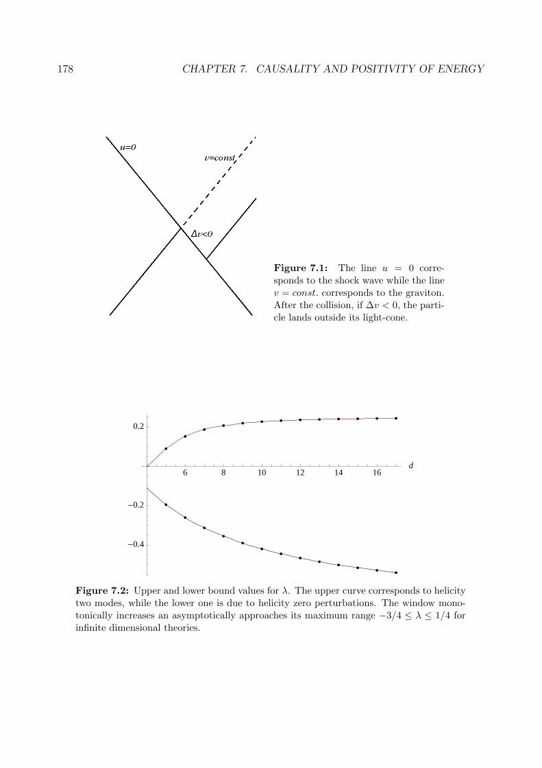
178 CHAPTER 7. CAUSALITY AND POSITIVITY OF ENERGY
Figure 7.1: The line u = 0 corre-sponds to the shock wave while the linev = const. corresponds to the graviton.After the collision, if ∆v < 0, the parti-cle lands outside its light-cone.
6 8 10 12 14 16d
-0.4
-0.2
0.2
Figure 7.2: Upper and lower bound values for λ. The upper curve corresponds to helicitytwo modes, while the lower one is due to helicity zero perturbations. The window mono-tonically increases an asymptotically approaches its maximum range −3/4 ≤ λ ≤ 1/4 forinfinite dimensional theories.
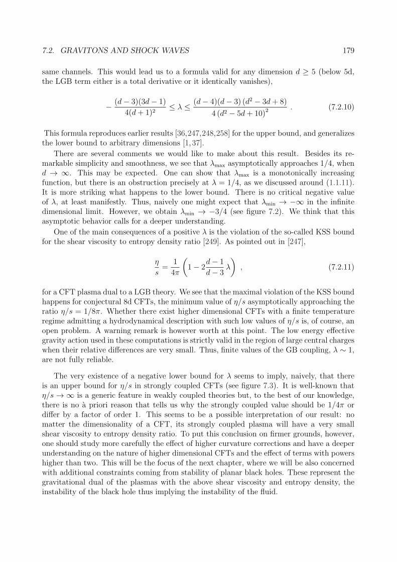
7.2. GRAVITONS AND SHOCK WAVES 179
same channels. This would lead us to a formula valid for any dimension d ≥ 5 (below 5d,the LGB term either is a total derivative or it identically vanishes),
− (d− 3)(3d− 1)
4(d+ 1)2≤ λ ≤ (d− 4)(d− 3) (d2 − 3d+ 8)
4 (d2 − 5d+ 10)2 . (7.2.10)
This formula reproduces earlier results [36,247,248,258] for the upper bound, and generalizesthe lower bound to arbitrary dimensions [1, 37].
There are several comments we would like to make about this result. Besides its re-markable simplicity and smoothness, we see that λmax asymptotically approaches 1/4, whend → ∞. This may be expected. One can show that λmax is a monotonically increasingfunction, but there is an obstruction precisely at λ = 1/4, as we discussed around (1.1.11).It is more striking what happens to the lower bound. There is no critical negative valueof λ, at least manifestly. Thus, naively one might expect that λmin → −∞ in the infinitedimensional limit. However, we obtain λmin → −3/4 (see figure 7.2). We think that thisasymptotic behavior calls for a deeper understanding.
One of the main consequences of a positive λ is the violation of the so-called KSS boundfor the shear viscosity to entropy density ratio [249]. As pointed out in [247],
η
s=
1
4π
(1− 2
d− 1
d− 3λ
), (7.2.11)
for a CFT plasma dual to a LGB theory. We see that the maximal violation of the KSS boundhappens for conjectural 8d CFTs, the minimum value of η/s asymptotically approaching theratio η/s = 1/8π. Whether there exist higher dimensional CFTs with a finite temperatureregime admitting a hydrodynamical description with such low values of η/s is, of course, anopen problem. A warning remark is however worth at this point. The low energy effectivegravity action used in these computations is strictly valid in the region of large central chargeswhen their relative differences are very small. Thus, finite values of the GB coupling, λ ∼ 1,are not fully reliable.
The very existence of a negative lower bound for λ seems to imply, naively, that thereis an upper bound for η/s in strongly coupled CFTs (see figure 7.3). It is well-known thatη/s→∞ is a generic feature in weakly coupled theories but, to the best of our knowledge,there is no a priori reason that tells us why the strongly coupled value should be 1/4π ordiffer by a factor of order 1. This seems to be a possible interpretation of our result: nomatter the dimensionality of a CFT, its strongly coupled plasma will have a very smallshear viscosity to entropy density ratio. To put this conclusion on firmer grounds, however,one should study more carefully the effect of higher curvature corrections and have a deeperunderstanding on the nature of higher dimensional CFTs and the effect of terms with powershigher than two. This will be the focus of the next chapter, where we will be also concernedwith additional constraints coming from stability of planar black holes. These represent thegravitational dual of the plasmas with the above shear viscosity and entropy density, theinstability of the black hole thus implying the instability of the fluid.
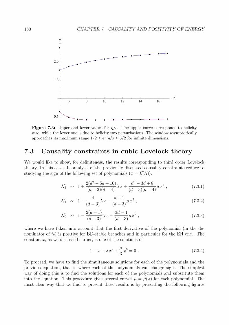
180 CHAPTER 7. CAUSALITY AND POSITIVITY OF ENERGY
6 8 10 12 14 16d
0.5
1.5
2.0
Η
s
Figure 7.3: Upper and lower values for η/s. The upper curve corresponds to helicityzero, while the lower one is due to helicity two perturbations. The window asymptoticallyapproaches its maximum range 1/2 ≤ 4π η/s ≤ 5/2 for infinite dimensions.
7.3 Causality constraints in cubic Lovelock theory
We would like to show, for definiteness, the results corresponding to third order Lovelocktheory. In this case, the analysis of the previously discussed causality constraints reduce tostudying the sign of the following set of polynomials (x = L2Λ)):
N2 ∼ 1 +2(d2 − 5d+ 10)
(d− 3)(d− 4)λx+
d2 − 3d+ 8
(d− 3)(d− 4)µx2 , (7.3.1)
N1 ∼ 1− 4
(d− 3)λx− d+ 1
(d− 3)µx2 , (7.3.2)
N0 ∼ 1− 2(d+ 1)
(d− 3)λx− 3d− 1
(d− 3)µx2 , (7.3.3)
where we have taken into account that the first derivative of the polynomial (in the de-nominator of t2) is positive for BD-stable branches and in particular for the EH one. Theconstant x, as we discussed earlier, is one of the solutions of
1 + x+ λx2 +µ
3x3 = 0 . (7.3.4)
To proceed, we have to find the simultaneous solutions for each of the polynomials and theprevious equation, that is where each of the polynomials can change sign. The simplestway of doing this is to find the solutions for each of the polynomials and substitute theminto the equation. This procedure gives several curves µ = µ(λ) for each polynomial. Themost clear way that we find to present these results is by presenting the following figures
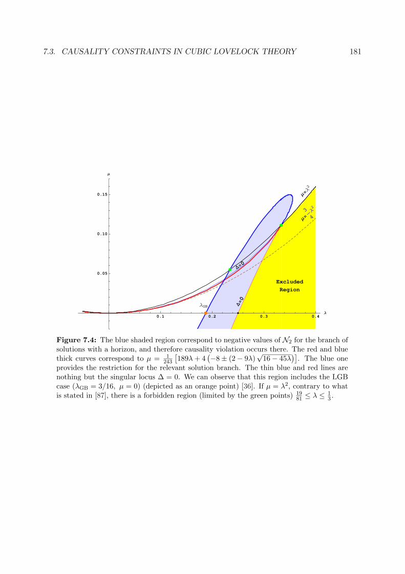
7.3. CAUSALITY CONSTRAINTS IN CUBIC LOVELOCK THEORY 181
0.1 0.2 0.3 0.4Λ
0.05
0.10
0.15
Μ
ΛGB
Μ=Λ2
Μ=
34Λ2
D=0
D=0
Excluded
Region
Figure 7.4: The blue shaded region correspond to negative values of N2 for the branch ofsolutions with a horizon, and therefore causality violation occurs there. The red and bluethick curves correspond to µ = 1
243
[189λ+ 4
(−8± (2− 9λ)
√16− 45λ
)]. The blue one
provides the restriction for the relevant solution branch. The thin blue and red lines arenothing but the singular locus ∆ = 0. We can observe that this region includes the LGBcase (λGB = 3/16, µ = 0) (depicted as an orange point) [36]. If µ = λ2, contrary to whatis stated in [87], there is a forbidden region (limited by the green points) 19
81 ≤ λ ≤13 .

182 CHAPTER 7. CAUSALITY AND POSITIVITY OF ENERGY
-2.0 -1.5 -1.0 -0.5 0.5Λ
-0.2
0.2
0.4
0.6
0.8Μ
ΛGB
Μ=Λ2
Μ=3
4Λ2
D=0
D=0
ExcludedRegion
Figure 7.5: The helicity 1 polynomial restrict the parameters to lie inside the regionbetween the blue curve and the excluded region. The shaded region correspond again tonegative values of N1 for the EH branch and thus to causality violation. The equationof the curve is µ = 1
144
[−18λ+ 49± (7 + 6λ)
√49− 120λ
]. For LGB gravity we found,
λ > −2.
which illustrate the situation. The analytic expression of the curves can be easily obtainedand, indeed, are discussed in the captions. We will discuss in the text their main qualitativefeatures.
In figure 7.4 we display both the region of the coupling space excluded by the argumentsof the preceding section and (in blue) the sector of the (λ, µ)-plane that leads to causalityviolation in the 7d Lovelock theory. Projected in the λ axis we reobtain the upper boundcorresponding to LGB gravity and obtained in [1, 36]. Even if, from the point of view ofAdS/CFT, the trustable region is close to the origin, i.e., for small values of λ and µ, it isamusing to see that the forbidden region has a structure that seems to be meaningful, evenif this is not fully justified. Notice that, had we restricted to third order Lovelock theorywith µ = λ2, we would have obtained a higher upper bound for λ (this corrects a misleadingstatement in [87]). Indeed, notice that there is a disconnected (from the Einstein-Hilberttheory) region since some finite positive values of λ are prevented by causality.
We represented the situation corresponding to helicity one gravitons colliding a shockwave or, alternatively, helicity one perturbations of the AdS black hole background in figure7.5. We see that it gives a complementary restriction in the coupling space. Again, itintersects the λ axis at the point −2, as obtained in [1]. We will not extend much in thediscussion of this curve for reasons that will be clear immediately.
Let us finally explore the causality violation induced by helicity zero gravitons. A veryimportant feature is the fact that this curve imposes more severe restrictions than thoseforced by the helicity one case. Indeed, the curve fully overcomes the helicity one constraints
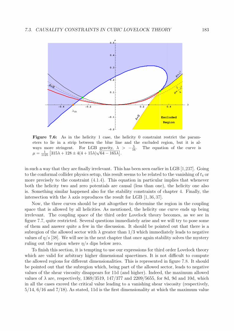
7.3. CAUSALITY CONSTRAINTS IN CUBIC LOVELOCK THEORY 183
-0.4 -0.2 0.2 0.4Λ
-0.2
-0.1
0.1
0.2
0.3
0.4
0.5Μ
ΛGB
Μ=Λ2
Μ=
3
4Λ2
D=0
D=0
Excluded
Region
Figure 7.6: As in the helicity 1 case, the helicity 0 constraint restrict the param-eters to lie in a strip between the blue line and the excluded region, but it is al-ways more stringent. For LGB gravity, λ > − 5
16 . The equation of the curve isµ = 1
1125
[315λ+ 128± 4(4 + 15λ)
√64− 165λ
].
in such a way that they are finally irrelevant. This has been seen earlier in LGB [1,237]. Goingto the conformal collider physics setup, this result seems to be related to the vanishing of t4 ormore precisely to the constraint (4.1.4). This equation in particular implies that wheneverboth the helicity two and zero potentials are causal (less than one), the helicity one alsois. Something similar happened also for the stability constraints of chapter 4. Finally, theintersection with the λ axis reproduces the result for LGB [1,36,37].
Now, the three curves should be put altogether to determine the region in the couplingspace that is allowed by all helicities. As mentioned, the helicity one curve ends up beingirrelevant. The coupling space of the third order Lovelock theory becomes, as we see infigure 7.7, quite restricted. Several questions immediately arise and we will try to pose someof them and answer quite a few in the discussion. It should be pointed out that there is asubregion of the allowed sector with λ greater than 1/3 which immediately leads to negativevalues of η/s [38]. We will see in the next chapter that once again stability solves the mysteryruling out the region where η/s dips below zero.
To finish this section, it is tempting to use our expressions for third order Lovelock theorywhich are valid for arbitrary higher dimensional spacetimes. It is not difficult to computethe allowed regions for different dimensionalities. This is represented in figure 7.8. It shouldbe pointed out that the subregion which, being part of the allowed sector, leads to negativevalues of the shear viscosity disappears for 11d (and higher). Indeed, the maximum allowedvalues of λ are, respectively, 1369/3519, 147/377 and 2209/5655, for 8d, 9d and 10d, whichin all the cases exceed the critical value leading to a vanishing shear viscosity (respectively,5/14, 6/16 and 7/18). As stated, 11d is the first dimensionality at which the maximum value
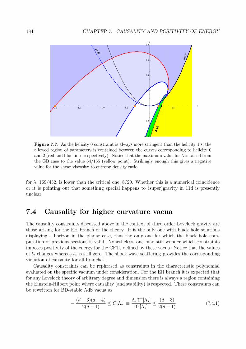
184 CHAPTER 7. CAUSALITY AND POSITIVITY OF ENERGY
-2.0 -1.5 -1.0 -0.5 0.5Λ
-0.4
-0.2
0.2
0.4
0.6
0.8Μ
Μ=
Λ2
D=
0
D=
0Figure 7.7: As the helicity 0 constraint is always more stringent than the helicity 1’s, theallowed region of parameters is contained between the curves corresponding to helicity 0and 2 (red and blue lines respectively). Notice that the maximum value for λ is raised fromthe GB case to the value 64/165 (yellow point). Strikingly enough this gives a negativevalue for the shear viscosity to entropy density ratio.
for λ, 169/432, is lower than the critical one, 8/20. Whether this is a numerical coincidenceor it is pointing out that something special happens to (super)gravity in 11d is presentlyunclear.
7.4 Causality for higher curvature vacua
The causality constraints discussed above in the context of third order Lovelock gravity arethose arising for the EH branch of the theory. It is the only one with black hole solutionsdisplaying a horizon in the planar case, thus the only one for which the black hole com-putation of previous sections is valid. Nonetheless, one may still wonder which constraintsimposes positivity of the energy for the CFTs defined by these vacua. Notice that the valuesof t2 changes whereas t4 is still zero. The shock wave scattering provides the correspondingviolation of causality for all branches.
Causality constraints can be rephrased as constraints in the characteristic polynomialevaluated on the specific vacuum under consideration. For the EH branch it is expected thatfor any Lovelock theory of arbitrary degree and dimension there is always a region containingthe Einstein-Hilbert point where causality (and stability) is respected. These constraints canbe rewritten for BD-stable AdS vacua as
− (d− 3)(d− 4)
2(d− 1)≤ C[Λ?] ≡
Λ?Υ′′[Λ?]
Υ′[Λ?]≤ (d− 3)
2(d− 1)(7.4.1)
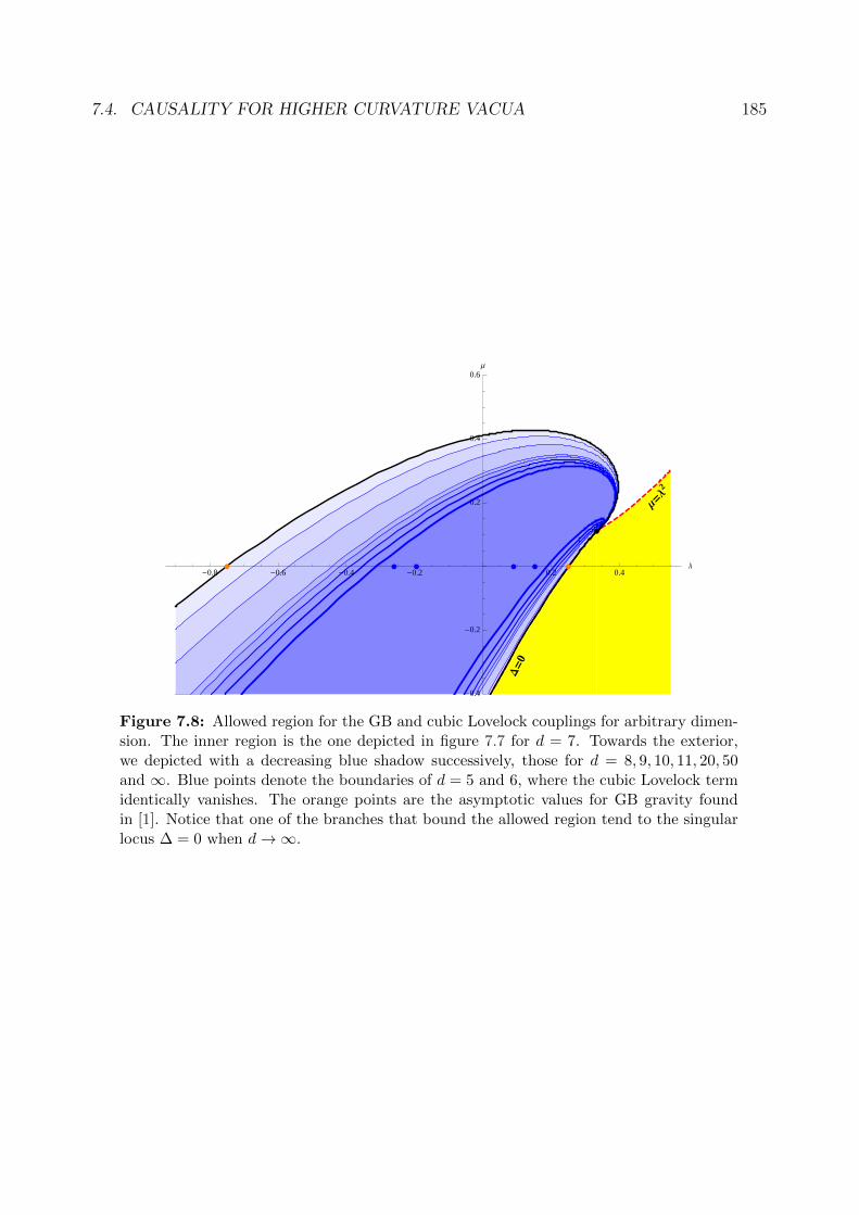
7.4. CAUSALITY FOR HIGHER CURVATURE VACUA 185
-0.8 -0.6 -0.4 -0.2 0.2 0.4Λ
-0.4
-0.2
0.2
0.4
0.6Μ
Μ=
Λ2
D=
0
Figure 7.8: Allowed region for the GB and cubic Lovelock couplings for arbitrary dimen-sion. The inner region is the one depicted in figure 7.7 for d = 7. Towards the exterior,we depicted with a decreasing blue shadow successively, those for d = 8, 9, 10, 11, 20, 50and ∞. Blue points denote the boundaries of d = 5 and 6, where the cubic Lovelock termidentically vanishes. The orange points are the asymptotic values for GB gravity foundin [1]. Notice that one of the branches that bound the allowed region tend to the singularlocus ∆ = 0 when d→∞.
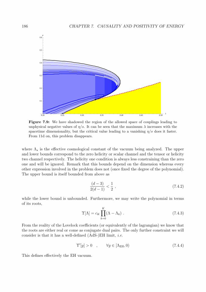
186 CHAPTER 7. CAUSALITY AND POSITIVITY OF ENERGY
0.20 0.25 0.30 0.35 0.40 0.45 0.50Λ
0.1
0.2
0.3
0.4
0.5
0.6Μ
Figure 7.9: We have shadowed the region of the allowed space of couplings leading tounphysical negative values of η/s. It can be seen that the maximum λ increases with thespacetime dimensionality, but the critical value leading to a vanishing η/s does it faster.From 11d on, this problem disappears.
where Λ? is the effective cosmological constant of the vacuum being analyzed. The upperand lower bounds correspond to the zero helicity or scalar channel and the tensor or helicitytwo channel respectively. The helicity one condition is always less constraining than the zeroone and will be ignored. Remark that this bounds depend on the dimension whereas everyother expression involved in the problem does not (once fixed the degree of the polynomial).The upper bound is itself bounded from above as
(d− 3)
2(d− 1)<
1
2, (7.4.2)
while the lower bound is unbounded. Furthermore, we may write the polynomial in termsof its roots,
Υ[Λ] = cK
K∏k=0
(Λ− Λk) . (7.4.3)
From the reality of the Lovelock coefficients (or equivalently of the lagrangian) we know thatthe roots are either real or come as conjugate dual pairs. The only further constraint we willconsider is that it has a well-defined (AdS-)EH limit, i.e.
Υ′[g] > 0 , ∀g ∈ [ΛEH, 0) (7.4.4)
This defines effectively the EH vacuum.
7.4. CAUSALITY FOR HIGHER CURVATURE VACUA 187
From the equivalent polynomial (7.4.3) we can very easily express C[Λi] for each vacuumas
C[Λi] = 2∑j 6=i
1
1− ΛjΛi
(7.4.5)
Also the Boulware-Deser stability of such vacuum can be very easily assessed in this way asthe first derivative of the polynomial there yields
Υ′[Λi] = cK∏j 6=i
(Λi − Λj) (7.4.6)
Starting from the stable EH-vacuum the AdS roots follow a series of stable/unstable vacuawhere complex conjugate pairs of roots do not matter. The same happens for the dS vacua.
For Λi < 0 we can classify the contributions to (7.4.5) according to their sign
1− Λj
Λi
> 0 ⇔ Λi ≤ Λj (7.4.7)
and the reverse for the opposite sign. This is also valid for the complex conjugate pairswhere Λj has to be replaced by its real part.
Using this it is very easy to show that in cubic Lovelock gravity, the minimal examplewith two BD-stable AdS-vacua, just the EH-vacua may be causal. In the case in which bothsuch vacua exist the characteristic polynomial displays three real roots
ΛHC < Λu < ΛEH < 0 (7.4.8)
where the subindices stand for higher curvature, unstable and Einstein-Hilbert respectively.If we want to analyze causality for the higher curvature vacuum ΛHC we have just to analyzetwo terms, both positive and bounded from below
C[ΛHC] =2
1− ΛuΛHC
+2
1− ΛEH
ΛHC
> 4 (7.4.9)
in such a way that C[ΛHC ] automatically violates the helicity zero (also the helicity one)constraint. The same happens for the smaller root of the polynomial when real. Assumingthere is at least one real AdS root (for instance the EH one) and that the rest has biggerreal part we can easily show
C[Λsmaller] > 2 (7.4.10)
In case there is any smaller root – with more negative real part – this would yield a neg-ative contribution to C[Λi]. In absolute value, this term may be as big as one wants, thecorresponding (unstable) vacuum just has to approach sufficiently the one we are analyzing.Thus, one negative term alone may compensate any positive contribution from the rest ofthe roots and bring the value of C[Λi] to the interval allowed by causality.
The minimal example for which we may have a BD-stable and causal AdS vacuum inaddition to the EH one is quartic Lovelock, we just need c4 > 0 in the region of parameterspace where the four roots are real and negative.
188 CHAPTER 7. CAUSALITY AND POSITIVITY OF ENERGY
7.5 Discussion
We have used the AdS/CFT framework to scrutinize higher order Lovelock theory in arbi-trary dimensions with the focus on possible causality violation. We have formally addressedthe more general case and explicitly worked out third order Lovelock gravity. Results forhigher order theories are contained in our formulas though some extra work is needed toextract them explicitly. Provided with the values of t2 and t4 appearing in the Maldacena-Hofman parametrization of the 3-point function of the stress tensor [234], we have checkedthe complete equivalence between the constraints arising from the positivity of energy boundsconjectured in that paper and those coming from causality. These results constitute a proofof previous conjectures in the literature [2, 239].
We do this computation in two different ways and end up showing that they are bound togive the same result. We have first computed all polarization linear perturbations of the blackhole AdS solution in Lovelock theory, and subsequently studied the collision of gravitons andshock waves in AdS in the framework of this theory. We found a region in the coupling spacewhere the theory does not violate causality (at least in a way that can be detected by thiskind of computations6). This generalizes the intervals found for λ in the case of LGB theories[1, 36, 237, 251]. Contrary to those intervals, that are now just given by the intersection ofthe allowed sector and the λ axis, the region is unbounded. Arbitrary large (simultaneous)negative values for λ and µ are allowed. The meaning of this result is unclear since thishappens in a region of couplings where the computations are not trustable. However, theregular pattern that we found as a function of the spacetime dimensionality is too niceto be discarded so easily. We have seen that the allowed region increases with spacetimedimensionality, as it happened with the LGB coupling [1]. In the infinite dimensional limit,one of the boundaries of the allowed region (roughly speaking, the one giving the upperbound; rigorously speaking, the one due to helicity two gravitons), asymptotically approachesthe zero discriminant boundary in the coupling space of the theory. This is expected sincethe region beyond that curve is excluded. The other curve, arising from scalar gravitons, hasa less natural behavior that calls for a deeper explanation. There is no restriction for thiscurve to be asymptotically larger, but it approaches a finite curve, that of course crosses theλ axis at λ = −3/4, in accordance with [1]. Thus, moderate (non-negative) values of λ andµ are forbidden even for would be infinite dimensional theories. Whether this is an artefactof our approach or there is a deeper reason for this behavior, is unclear to us at this point.
It is intriguing that classical Lovelock gravity in AdS space can capture highly non-trivialaspects of conformal field theory physics. While Einstein gravity is known to describe theuniversal spin-2 sector of a large class of strongly coupled CFTs, no dual to Lovelock gravity(beyond GB) has been found, nor have the Lovelock terms with finite coefficients appearedin string theory. While higher powers of curvature generically appear in string theory asα′ corrections to the supergravity action, these corrections are necessarily perturbative. InLovelock theory, we have dimensionful parameters appearing in the lagrangian which do notappear to be protected from quantum corrections by any symmetry. That from the classi-cal theory we can obtain specific numerical predictions on which values of the parametersshould or not be allowed by causality and that these restrictions should agree with analogous
6§ Tighter constraints may arise in case we change the shock wave profile (see for instance [10]).
7.5. DISCUSSION 189
restrictions in a hypothetical dual CFTs is highly suggestive. We obtain what seem to besplendid checks of the AdS/CFT correspondence, the results being smooth functions of thespacetime dimensionality.
One possible hint is that Lovelock theories all satisfy t4 = 0, which is required for super-symmetric CFTs [259]. For free field theories, t4 = 0 is obtained by picking the appropriatesupersymmetric matter content. In Lovelock gravity, the t2 and t4 parameters can be ob-tained in the boundary expansions of the effective potentials (4.1.3). The t4 = 0 result shouldimply some relationship between these. Indeed, it is easy to see that from (4.1.3) we have
(d− 4) c22(r) + (d− 2) c2
0(r)− 2(d− 3) c21(r) = 0 , (7.5.1)
which is actually valid at any radius r and not just at the boundary, where it indeed impliest4 = 0. Beyond the boundary expansion, the relationship written above should imposeconstraints on higher n-point functions of the theory. It is tempting to conjecture that theseare the holographic duals of some sort of supersymmetric constraint.
The papers that originally dealt with causality violation did it under the spell of searchingpossible violations of the KSS bound [247,248]. They found that the addition of a LGB termin the gravity lagrangian corrects the universal value of the shear viscosity to entropy densityratio as
η
s=
1
4π(1− 4λ) . (7.5.2)
The addition of further higher order Lovelock terms does not manifestly contribute to thisquotient [250]. The possible addition of a quadratic curvature correction with positive λ isenough to argue that the KSS bound is not universally valid. The appearance of an upperbound for λ due to causality conservation naively seems to lower the KSS bound down toa new one. Since (7.5.2) is not affected by higher order Lovelock terms, this has led someauthors to speculate about the nature of this newly found lower bound. However, it is notclear if the new bound should be taken seriously: when λ approaches the maximal allowedvalue, the central charges of the dual CFT explore a regime (roughly (a − c)/c ∼ O(1))where the gravity description is a priori untrustable. Furthermore, let us point out that thefact that higher order Lovelock couplings do not enter (7.5.2) does not mean that they areirrelevant for this problem. Indeed, we have seen that even an infinitesimal positive valueof µ would raise the upper bound for λ thus affecting the putative lower bound for η/s.Even more weird, there are values of µ leading to too high values of λ in the sense thatη/s becomes negative. We will see in the next chapter that the mechanism allowing us todisregard this unphysical behavior is actually the stability of the plasma, dual to the stabilityof planar black holes studied in chapter 4. These additional constraints will further restrictthe possible values of the Lovelock coefficients being crucial for the discussion of bounds onη/s.
Previously, concerning the LGB case, it was raised the issue about the string theoryorigin of quadratic curvature corrections. It seems clear after [229,230,255] that these termsmay possibly arise from D-brane probes or AN−1 singularities in M-theory. The situationwith the cubic curvature corrections is more delicate in this respect. Besides, the very factthat the results generalize smoothly both to higher order Lovelock theory and to higherspacetime dimensions, seems to suggest that these computations may not necessarily rely inthe framework of string theory.
190 CHAPTER 7. CAUSALITY AND POSITIVITY OF ENERGY
Our results for arbitrary dimensions are compatible with the condition t4 = 0. This isthe expected value of t4 for a supersymmetric CFT. Cubic terms are expected to accomplishsupersymmetry breaking. However, this is not the case for the Lovelock combination. As fort2, the result of this chapter is unexpected. It is well-known that the third order Lovelockterm endows a 3-graviton vertex structure that does not contribute to the 3-point function[257]. However, this result is strictly valid for flat space-times while in AdS, as we see, itis not true. The introduction of the third order Lovelock lagrangian enters non-trivially inthe discussion of causality violation. It would be interesting to further clarify how this termcontributes to t2 by studying directly the 3-graviton vertex in AdS spacetimes.
Chapter 8
Holographic plasmas and the fate ofthe viscosity bound
“A poet once said, ‘The whole universe is in a glass of wine’.We will probably never know in what sense he meant that,
for poets do not write to be understood. But it is true that if welook at a glass of wine closely enough we see the entire universe.”
Richard Feynman
The AdS/CFT correspondence has provided a tool to study hydrodynamical aspects ofquantum field theories at strong coupling. This was particularly timely due to the adventof experiments that prompted the exploration of QCD in a region of phase space where itdisplays such behavior. One of the most striking predictions of AdS/CFT had to do with theshear viscosity to entropy density ratio, η/s, of strongly coupled plasmas. Policastro, Son andStarinets computed this ratio in the canonical example of N = 4 SU(N) supersymmetricYang-Mills (SYM) plasma, in the planar (’t Hooft) limit and for infinitely large ’t Hooftcoupling λ = g2
YM N →∞ [260], finding
η
s=
1
4π(8.0.1)
Interestingly enough, it was found that there is a universal value for this ratio, η/s = 1/4π,for theories whose gravity dual is governed by the Einstein–Hilbert action, regardless ofthe matter content, the number of supersymmetries, the existence or not of a conformalsymmetry, and even the spacetime dimensionality. On the other hand, all measured valuesfor this ratio in any quantum relativistic system are above this value. This led to speculationsthat η/s ≥ 1/4π might be an exact statement in quantum relativistic systems, the so-called
191
192 CHAPTER 8. THE FATE OF THE VISCOSITY BOUND
KSS bound conjecture [249]. Indeed, it is possible to provide a hand waving argument[261], relying on a quasiparticle description of the plasma, that links the KSS bound to theHeisenberg uncertainty principle. This argument is questionable, though, since there areconvincing hints supporting a non-quasiparticle description of strongly interacting plasmas.
The KSS bound conjecture has been thoroughly scrutinized for many years (see, forexample, [262] for a recent review). It turned out to be the case, however, that whenquantum corrections are included in the gravitational action, under the form of curvaturesquared terms, the η/s ratio can be smaller than the KSS bound [229, 247]. In particular,there are string theory constructions where this is the case [229,230]. In these situations theviolation of the viscosity bound can be traced back to the inequality between the centralcharges of the theory, namely to c−a > 0, quite generic in superconformal gauge theories withunequal central charges [230]. Moreover, to ensure reliable computations, higher curvaturecorrections have to be regarded as being small. As a result, any violation of the KSS boundrealized in string models of the duality is necessarily perturbative. Nonetheless, the questionof the existence of any such bound persisted. Because of the universality property of theshear viscosity to entropy density in the supergravity approximation, any finite violation ofthe KSS bound has to be studied in an effective model of AdS/CFT, rather than a particularrealization of the correspondence in string theory.
For the particular combination given by the LGB term, one may consider finite valuesof the coefficient, as the gravitational theory is then two-derivative. As such, it effectivelydefines via the AdS/CFT correspondence a dual conformal plasma. For this we can compute2- and 3-point function as discussed in chapter 6 and also transport coefficients such as η/s.In this case the ratio is modified to [263,264]
η
s=
1
4π
(1− 2(d− 1)
d− 3λ
), (8.0.2)
λ being the appropriately normalized LGB coupling, and the KSS bound is violated wheneverλ is positive [229, 247]. Up to field redefinitions, for very small λ the gravitational modelwith a LGB correction is equivalent to the example of Kats and Petrov [229] embedded instring theory. For that we have to identify
c− ac∼ λ (8.0.3)
that now can be taken however to finite values.Even if a priori the addition of a LGB term would lead to an arbitrary violation of the
KSS bound, it turns out that the causality constraints studied in the previous section arisepreventing the possibility of going to arbitrarily low values of η/s [248]. This was actuallythe original motivation of their discovery. In the case of 4d CFTs, for instance, this imposesthe constraint λ ≤ 9/100, which reduces the minimum value of η/s by a factor of 16/25.
The study of a possible bound is interesting both from a theoretical standpoint as wellas from a phenomenological one – it has been found experimentally that the quark-gluonplasma created in relativistic heavy ion collisions appears to have a very low shear viscos-ity to entropy density ratio [265]. A similar result was also found recently in a radicallydifferent context: that of strongly correlated ultracold atomic Fermi gasses in the so-called
193
unitarity limit [266]. Both systems have measured values of η/s compatible with 1/4π. Onthe other hand, from a theoretical standpoint, the causality constraints coming from thebehavior of the geometry near the boundary, that rule the attainability of lower values ofη/s, have a beautiful holographic dual in the CFT side: they arise from positivity of energyconditions [234, 237, 267]. The perfect matching of these two quite fundamental restrictionson a physically sensible theory constitutes a striking check of the AdS/CFT correspondence.
Whether this is still valid for higher-dimensional CFTs became a natural question thatwas subsequently answered in a series of papers [1,37,268]. Summarizing, it turned out thatLGB theories lead to a violation of the KSS bound in any spacetime dimensionality, and thatcausality constraints exactly match positivity of energy bounds on the CFT side. The factthat this matching is valid regardless of the dimensionality is puzzling and seems to provideclues on possible non-stringy versions of AdS/CFT. Our knowledge of higher-dimensionalCFTs is, however, too poor yet to push these arguments forward. In higher dimensions onehas in general the choice of including other Lovelock terms in the action. These are higherorder in curvature that still lead to second order equations of motion [15]. A first step inthe analysis of these theories was done in [2, 239]. There it was found that causality andpositivity of energy constraints still match perfectly. Still, something new happens here.Since there are now more free parameters available, it turns out that causality alone cannotprevent the η/s ratio from becoming arbitrarily small (or even negative).
In this chapter we analyze in detail the fate of the η/s ratio in AdS/CFT restrictedto the case of Lovelock theories. We will focus in the cases of LGB, cubic and quarticLovelock gravities in arbitrary dimension, even though general results are contained in ourformulas. We will study restrictions coming from positivity of energy correlators of theCFT, as explained in the previous chapter. We then consider graviton fluctuations aboutthe black hole background for a general Lovelock theory. Near the boundary, demandingcausality of graviton propagation leads to bounds which exactly match those of energy fluxpositivity. Close to the horizon, in turn, we have shown that unstable modes can appear ifthe parameters of the theory are not tuned properly. This leads to another set of boundswhich, for the LGB gravity or cubic Lovelock theory in seven dimensions, prevent the η/sratio from becoming arbitrarily small. In the case of higher order Lovelock theories, a newphenomenon occurs1: causality violation and plasma instabilities may arise in the interiorof the geometry. They should be related to analogous unhealthy properties arising in theCFT plasma far from the UV, whose identification and full characterization is left as anopen problem. Causality violations and instabilities should have, however, very differentphysical interpretations: while we may expect that the former correspond to some illness ofthe boundary theory, the latter should be related to either plasma instabilities or to issuessuch as not being expanding around the true vacuum2. Anyway, interestingly enough, thisshows that causality violation is not necessarily a phenomenon arising in the UV and it isnot generically dual to positivity of energy in the CFT.
The attentive reader has already realized that higher order Lovelock gravities imply
1This phenomenon already takes place for the cubic Lovelock theory. It leads to a less stringent (thusirrelevant) constraint in d = 7, but is crucial to prevent arbitrarily small values of η/s in 8 ≤ d ≤ 10 theories.When d > 10, causality at the boundary is enough to discard this possibility in cubic Lovelock gravity [2].
2We thank Rob Myers for clarifying comments on these points.
194 CHAPTER 8. THE FATE OF THE VISCOSITY BOUND
higher-dimensional theories. There is a second more subtle point that should be presentlyraised. The analysis performed in this chapter deals with higher order curvature correctionswhose coupling constants do not need to be necessarily small. Both conditions are unnat-ural within the string theory realm. It seems however worth inspecting thoroughly thesetheories based on the very fact that they lead to reasonable results. That is, even for thesepresumably non-stringy setups we obtain what seem to be splendid checks of the AdS/CFTcorrespondence.
The last section is devoted to the analysis of the η/s ratio in higher order Lovelock theo-ries. The first part of that section presents analytic and numerical results for the minimumratio in any dimension up to quartic order theory. These are obtained by considering thefull stability and causality constraints. Our results are relatively smooth functions of thespacetime dimensionality. We also show that for any given Lovelock theory of order K thereis always a lower bound on η/s. It is impossible to get arbitrarily close to η/s = 0, evenin the case where the causality constraints would not be taken into account as proposedin [269].
In the second part we consider a limited analysis of arbitrary Lovelock theories in anydimension. Picking a specific curve through parameter space, the properties of which arecarefully discussed in Appendix C, we show that there seems not to be a dimension inde-pendent viscosity bound. Within our framework, we argue that a strongly coupled idealfluid could be achieved in the strict limit d→∞, when a correspondingly infinite number ofLovelock terms are taken into account. This is somehow reminiscent of the so-called speciesproblem, although it is not clear to us whether there is a more rigorous way in which thesetwo setups are related.
8.1 Shear viscosity and finite temperature instabilities
It has been shown in [263,264] that the shear viscosity to entropy ratio of a generic Lovelocktheory is given by
η
s=
1
4π
(1− λ
λc
), (8.1.1)
where we have defined the critical value λc where the ratio vanishes
λc ≡d− 3
2(d− 1). (8.1.2)
It is interesting to stress that the ratio only depends on the quadratic Lovelock coupling,c2. Generically one is not free to take an arbitrary λ. There are causality constraints whichrestrict the range of values where the theory is well defined [247, 248]. These restrictionsmatch the restrictions on t2 and t4, and these necessarily involve all the parameters in thetheory. The maximum value λ(0) that may be achieved depends on the theory in question. Inthis way it has been found [2,239] that causality constraints alone cannot prevent one fromreaching (and even overpassing) η/s = 0. In this section we show that as one approachessmall values of η/s, the black hole becomes unstable and the linear approximation breaksdown. This places an effective set of constraints in the parameters of the theory, saving theratio above from ever becoming too small.
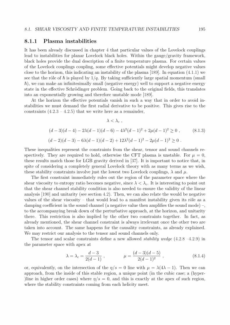
8.1. SHEAR VISCOSITY AND FINITE TEMPERATURE INSTABILITIES 195
8.1.1 Plasma instabilities
It has been already discussed in chapter 4 that particular values of the Lovelock couplingslead to instabilities for planar Lovelock black holes. Within the gauge/gravity framework,black holes provide the dual description of a finite temperature plasma. For certain valuesof the Lovelock couplings coupling, some effective potentials might develop negative valuesclose to the horizon, this indicating an instability of the plasma [189]. In equation (4.1.1) wesee that the role of ~ is played by 1/q. By taking sufficiently large spatial momentum (small~), we can make an infinitesimally small (negative energy) well to support a negative energystate in the effective Schrodinger problem. Going back to the original fields, this translatesinto an exponentially growing and therefore unstable mode [189].
At the horizon the effective potentials vanish in such a way that in order to avoid in-stabilities we must demand the first radial derivative to be positive. This gives rise to theconstraints (4.2.3 – 4.2.5) that we write here as a remainder,
λ < λc ,
(d− 3)(d− 4)− 2λ(d− 1)(d− 6)− 4λ2(d− 1)2 + 2µ(d− 1)2 ≥ 0 , (8.1.3)
(d− 2)(d− 3)− 6λ(d− 1)(d− 2) + 12λ2(d− 1)2 − 2µ(d− 1)2 ≥ 0 .
These inequalities represent the constraints from the shear, tensor and sound channels re-spectively. They are required to hold, otherwise the CFT plasma is unstable. For µ = 0,these results match those for LGB gravity derived in [37]. It is important to notice that, inspite of considering a completely general Lovelock theory with as many terms as we wish,these stability constraints involve just the lowest two Lovelock couplings, λ and µ.
The first constraint immediately rules out the region of the parameter space where theshear viscosity to entropy ratio becomes negative, since λ < λc. It is interesting to point outthat the shear channel stability condition is also needed to ensure the validity of the linearanalysis [190] and unitarity (see section 4.2). Then, we can also relate the would be negativevalues of the shear viscosity – that would lead to a manifest instability given its role as adamping coefficient in the sound channel (a negative value then amplifies the sound mode) –,to the accompanying break down of the perturbative approach, at the horizon, and unitaritythere. This restriction is also implied by the other two constraints together. In fact, asalready mentioned, the shear channel constraint is always irrelevant once the other two aretaken into account. The same happens for the causality constraints, as already explained.We may restrict our analysis to the tensor and sound channels only.
The tensor and scalar constraints define a new allowed stability wedge (4.2.8 –4.2.9) inthe parameter space with apex at
λ = λc =d− 3
2(d− 1), µ =
(d− 3)(d− 5)
2(d− 1)2, (8.1.4)
or, equivalently, on the intersection of the η/s = 0 line with µ = λ(4λ − 1). Then we canapproach, from the inside of this stable region, a unique point (in the cubic case; a (hyper-)line in higher order cases) where η/s = 0, and this is exactly at the apex of such region,where the stability constraints coming from each helicity meet.
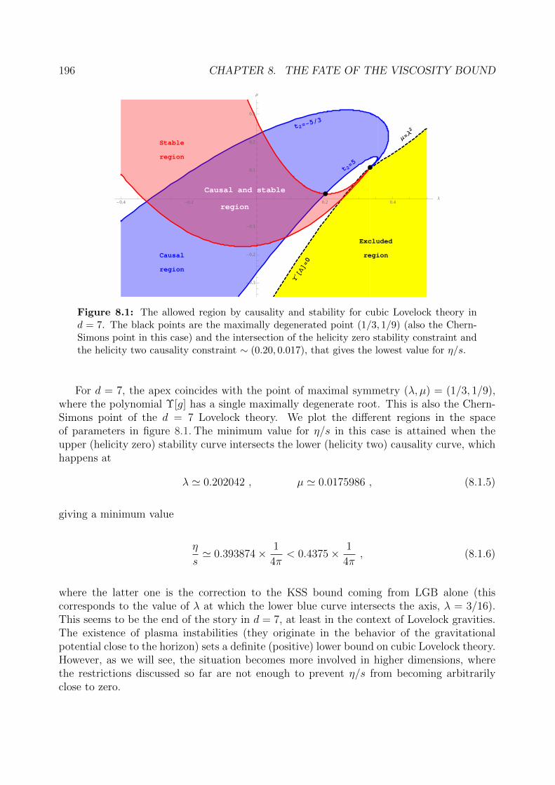
196 CHAPTER 8. THE FATE OF THE VISCOSITY BOUND
-0.4 -0.2 0.2 0.4Λ
-0.3
-0.2
-0.1
0.1
0.2
0.3
Μ
Causal
region
Stable
region
Causal and stable
region
Excluded
region
Μ=Λ2
U¢ @L
D=0
t2=5
t2=-53
Figure 8.1: The allowed region by causality and stability for cubic Lovelock theory ind = 7. The black points are the maximally degenerated point (1/3, 1/9) (also the Chern-Simons point in this case) and the intersection of the helicity zero stability constraint andthe helicity two causality constraint ∼ (0.20, 0.017), that gives the lowest value for η/s.
For d = 7, the apex coincides with the point of maximal symmetry (λ, µ) = (1/3, 1/9),where the polynomial Υ[g] has a single maximally degenerate root. This is also the Chern-Simons point of the d = 7 Lovelock theory. We plot the different regions in the spaceof parameters in figure 8.1. The minimum value for η/s in this case is attained when theupper (helicity zero) stability curve intersects the lower (helicity two) causality curve, whichhappens at
λ ' 0.202042 , µ ' 0.0175986 , (8.1.5)
giving a minimum value
η
s' 0.393874× 1
4π< 0.4375× 1
4π, (8.1.6)
where the latter one is the correction to the KSS bound coming from LGB alone (thiscorresponds to the value of λ at which the lower blue curve intersects the axis, λ = 3/16).This seems to be the end of the story in d = 7, at least in the context of Lovelock gravities.The existence of plasma instabilities (they originate in the behavior of the gravitationalpotential close to the horizon) sets a definite (positive) lower bound on cubic Lovelock theory.However, as we will see, the situation becomes more involved in higher dimensions, wherethe restrictions discussed so far are not enough to prevent η/s from becoming arbitrarilyclose to zero.

8.2. BULK CAUSALITY AND STABILITY 197
0.15 0.20 0.25 0.30 0.35 0.40Λ
0.1
0.2
0.3
0.4
Μ
0.28 0.30 0.32 0.34 0.36Λ
0.08
0.10
0.12
0.14
0.16
0.18
0.20
Μ
Figure 8.2: Causality and stability regions in d = 9 cubic Lovelock theory (and zoom).The thick lines correspond to causality at the boundary and stability at the horizon, re-spectively in blue and red, while the dashed lines correspond to causality (in the tensorchannel) and stability (in the sound channel) in the full geometry.
8.2 Bulk causality and stability
8.2.1 The cubic theory in higher dimensions
Our results imply that the η/s ratio can never be too small for cubic Lovelock theory ind = 7 by a combination of two constraints – preservation of causality, holographically dual topositivity of energy; and stability of the black brane solution which can be broadly identifiedwith the stability of the thermal plasma. Of course the obvious question is whether similarresults are valid in higher order theories. As it turns out, these two constraints are indeedenough, but not in the simple fashion we have described so far – we must require causalityand stability everywhere in the bulk, and not just from a simple near boundary or nearhorizon analysis.
This can be seen already in the simplest case of cubic Lovelock theory in higher dimen-sions. In figures 8.2 and 8.3 we show the relevant part of the causal and stable regions ford = 9 and d = 11, as determined by the near horizon and near boundary expansions of theeffective potentials. There are also a few dashed lines plotted whose meaning we will explainin a moment. It is apparent that by going to higher dimensions, a disconnected region closeto the apex of the stability region is now causal as well. This means that such a regionsatisfies all our previous constraints, and yet it will have an arbitrarily low shear viscosity.This is because, as we have seen earlier, the apex of the stability region actually lives on thesurface η = 0 determined by the stability constraint in the shear channel. This point liesinside the causality allowed region for d ≤ 10 [2].
While in principle there is nothing wrong with having a small ratio, this is not the endof the story. As we have mentioned before, by considering the full effective potentials wecan see that they develop causality problems and/or instabilities, but now in the interior ofthe black hole geometry (see figures 8.4).In the left figure, even though the potential initiallyrises close to the horizon (g = 0), it dips into negative values. In the same way, in thefigure on the right, the potential goes below one close to the boundary and then makes a
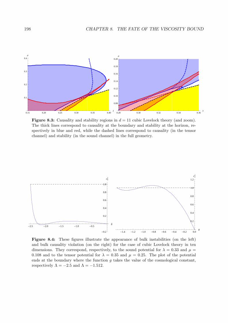
198 CHAPTER 8. THE FATE OF THE VISCOSITY BOUND
0.15 0.20 0.25 0.30 0.35 0.40Λ
0.1
0.2
0.3
0.4
Μ
0.28 0.30 0.32 0.34 0.36Λ
0.08
0.10
0.12
0.14
0.16
0.18
0.20
Μ
Figure 8.3: Causality and stability regions in d = 11 cubic Lovelock theory (and zoom).The thick lines correspond to causality at the boundary and stability at the horizon, re-spectively in blue and red, while the dashed lines correspond to causality (in the tensorchannel) and stability (in the sound channel) in the full geometry.
-2.5 -2.0 -1.5 -1.0 -0.5g
-0.2
0.2
0.4
0.6
0.8
1.0
c02
-1.4 -1.2 -1.0 -0.8 -0.6 -0.4 -0.2 0.0g
0.2
0.4
0.6
0.8
1.0
1.2
c22
Figure 8.4: These figures illustrate the appearance of bulk instabilities (on the left)and bulk causality violation (on the right) for the case of cubic Lovelock theory in tendimensions. They correspond, respectively, to the sound potential for λ = 0.33 and µ =0.108 and to the tensor potential for λ = 0.35 and µ = 0.25. The plot of the potentialends at the boundary where the function g takes the value of the cosmological constant,respectively Λ = −2.5 and Λ = −1.512.
8.2. BULK CAUSALITY AND STABILITY 199
hump above this value, leading to causality violation. Such features cannot be fully seen ina perturbative analysis, although their presence is easily guessed at. Consider for instancemoving along the curve where the causality bound is saturated in the tensor channel. Thismeans that the effective potential is of the form
Veff = 1 + 0× ex + v4 e2x + . . . (8.2.1)
It is clear then that along this curve we will see causality violation if v4 ever becomespositive. Beyond the point in parameter space where this occurs, there will be a competitionbetween the ex and e2x terms in the potential expansion which will determine the shape ofthe causality curve from that point onwards. In general it is clear that to determine thiscurve one must consider the full effective potential, since all terms in the near-boundaryexpansion become of the same order. Analogous statements hold for the instability analysisnear the horizon. These curves are determined numerically and shown as dashed lines infigures 8.2 and 8.3. We can see, in particular, that the sound mode instability curve neatlycuts off the region where η/s might become too small, thereby imposing an effective lowerbound on this ratio.
Going to higher order Lovelock theories, one may wonder if this general reasoning willhold. Could the addition of further couplings allow us to escape even the full causality andstability bounds? This does not seem to be so. Evidence for this conclusion comes from ananalysis of quartic Lovelock theory, to which we now turn.
8.2.2 Quartic Lovelock theory
Quartic theory corresponds to the introduction of an extra nonzero parameter, c4 ≡ ν4L6.
The theory exists in d ≥ 9, and examining it requires solving for quartic polynomials. Theanalysis of the parameter space of this theory is made in a somewhat similar manner to thecubic case, and we will not go into great detail here. There are resemblances and differencesto the cubic theory. For instance, as in the lower order cases the boundary of the excludedregion is just the surface where the cosmological constant associated with the EH branchbecomes degenerate. However, this surface ends at one of the triply degenerated lines (threecosmological constants equal) and we need another surface to actually close the excludedregion. This also happens in the cubic case where the excluded region is closed by µ = λ2,which is the line along which all three solutions become degenerate at some point inside thegeometry. In the quartic case the situation is analogous and the excluded region is closedby the surface swept by the line where three solutions degenerate at some value of theradius. This surface cuts off the other surfaces bounding the causal regions for the differenthelicities: green for tensor channel and dark blue for the sound. As always, the causal regionis contained between the tensor and sound surfaces (figure 8.5). Besides, we also realize thatthe values of λ are not bounded (neither from below nor from above) just due to causality– by increasing ν it is possible to go to arbitrarily high λ.
This situation drastically changes once we consider stability and causality constraints (seefigure 8.6). When horizon stability is imposed, the allowed region of parameters is furtherconstrained by the purple surfaces; notice, in particular, that it includes a channel connectingthe Einstein-Hilbert point with the η/s = 0 line (the apex of the stability region, in purple).
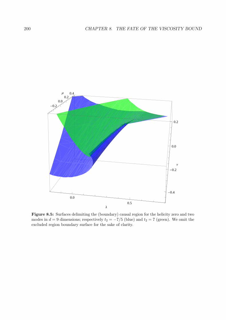
200 CHAPTER 8. THE FATE OF THE VISCOSITY BOUND
0.0
0.5Λ
-0.20.0
0.20.4Μ
-0.4
-0.2
0.0
0.2
Ν
Figure 8.5: Surfaces delimiting the (boundary) causal region for the helicity zero and twomodes in d = 9 dimensions; respectively t2 = −7/5 (blue) and t2 = 7 (green). We omit theexcluded region boundary surface for the sake of clarity.
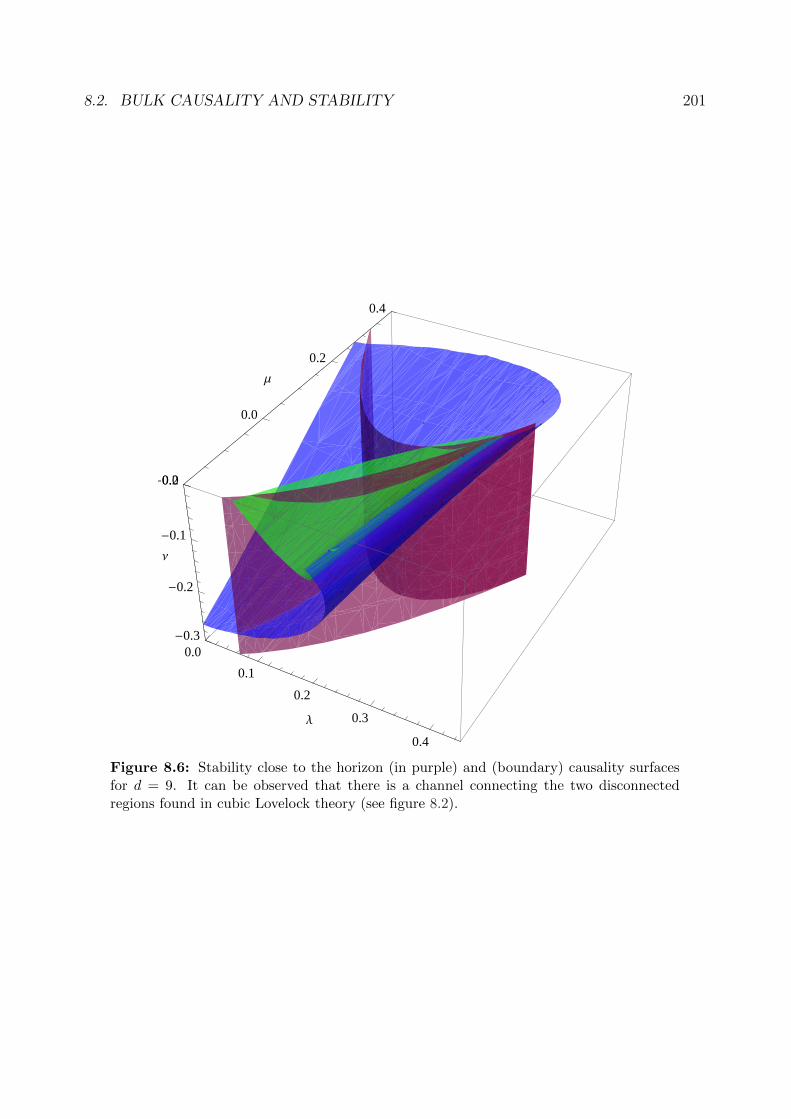
8.2. BULK CAUSALITY AND STABILITY 201
0.0
0.1
0.2
0.3
0.4
Λ
-0.2
0.0
0.2
0.4
Μ
-0.3
-0.2
-0.1
0.0
Ν
Figure 8.6: Stability close to the horizon (in purple) and (boundary) causality surfacesfor d = 9. It can be observed that there is a channel connecting the two disconnectedregions found in cubic Lovelock theory (see figure 8.2).
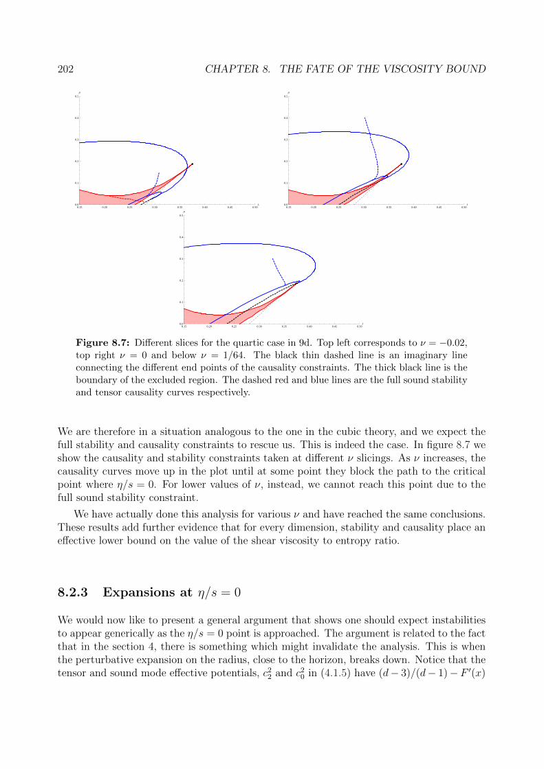
202 CHAPTER 8. THE FATE OF THE VISCOSITY BOUND
0.15 0.20 0.25 0.30 0.35 0.40 0.45 0.50Λ0.0
0.1
0.2
0.3
0.4
0.5
Μ
0.15 0.20 0.25 0.30 0.35 0.40 0.45 0.50Λ0.0
0.1
0.2
0.3
0.4
0.5
Μ
0.15 0.20 0.25 0.30 0.35 0.40 0.45 0.50Λ0.0
0.1
0.2
0.3
0.4
0.5
Μ
Figure 8.7: Different slices for the quartic case in 9d. Top left corresponds to ν = −0.02,top right ν = 0 and below ν = 1/64. The black thin dashed line is an imaginary lineconnecting the different end points of the causality constraints. The thick black line is theboundary of the excluded region. The dashed red and blue lines are the full sound stabilityand tensor causality curves respectively.
We are therefore in a situation analogous to the one in the cubic theory, and we expect thefull stability and causality constraints to rescue us. This is indeed the case. In figure 8.7 weshow the causality and stability constraints taken at different ν slicings. As ν increases, thecausality curves move up in the plot until at some point they block the path to the criticalpoint where η/s = 0. For lower values of ν, instead, we cannot reach this point due to thefull sound stability constraint.
We have actually done this analysis for various ν and have reached the same conclusions.These results add further evidence that for every dimension, stability and causality place aneffective lower bound on the value of the shear viscosity to entropy ratio.
8.2.3 Expansions at η/s = 0
We would now like to present a general argument that shows one should expect instabilitiesto appear generically as the η/s = 0 point is approached. The argument is related to the factthat in the section 4, there is something which might invalidate the analysis. This is whenthe perturbative expansion on the radius, close to the horizon, breaks down. Notice that thetensor and sound mode effective potentials, c2
2 and c20 in (4.1.5) have (d− 3)/(d− 1)−F ′(x)
8.2. BULK CAUSALITY AND STABILITY 203
in the denominator. At the horizon we have,
d− 3
d− 1− F ′(x) ' 2(λc − λ) . (8.2.2)
This means that the near-horizon expansion breaks down whenever λ ' λc, precisely whereη/s ' 0. Close enough to this point the previous approximation is no longer valid and wemust treat this case separately. This is true for any Lovelock theory in any dimension, andit is therefore of interest to see if there are any general statements one can make.
Let us then investigate the behavior of the effective potentials given in (4.1.3) at thehorizon. First notice that the black hole polynomial equation (2.1.8) fixes
g(x) ' x
L2+O(x2) , (8.2.3)
and we can expand(d− 3
d− 1− F ′(x)
)≈(d− 3
d− 1− F ′(0)
)−∑n=1
1
n!F (n+1)(0) xn . (8.2.4)
The expansion is such that each term in the above is controlled by a different Lovelockparameter. For instance F ′(0) = 2λ, and so the first term vanishes whenever λ = λc. Whenthe following derivatives F (j)(0) vanish, ∀j < n, we can actually write
F (n)(0) = Υ(n+1)[0]−n∏i=1
d− 2i− 1
d− 1, (8.2.5)
and so we can set the following term to zero by choosing
(cn+1)c =Υ(n)[0]
n!=
1
n!
n−1∏i=1
d− 2i− 1
d− 1. (8.2.6)
In particular,
µc =1
2
(d− 3)(d− 5)
(d− 1)2, νc =
1
6
(d− 3)(d− 5)(d− 7)
(d− 1)3, . . . (8.2.7)
For a given (odd) dimensional Lovelock theory, if we set all K = d−12
couplings to theseparticular values, we will be at the so-called AdS Chern-Simons point [43]. Now, noticethat (8.2.4) is actually the denominator of the helicity two and helicity zero potentials (andproportional to that of the helicity one mode). The leading correction to those potentialsclose to the horizon, when we set F ′(0) = 2λc and F (j<n)(0) = 0, is then
c22(x) ≈ −d− 1
d− 4
n− 1
L2 Λ+O(x) , (8.2.8)
c21(x) ≈ −d− 1
d− 3
F (n)(0)
(n− 1)!L2 Λxn (1 +O(x)) , (8.2.9)
c20(x) ≈ d− 1
d− 2
n− 1
L2 Λ+O(x) . (8.2.10)
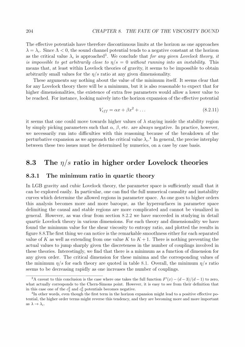
204 CHAPTER 8. THE FATE OF THE VISCOSITY BOUND
The effective potentials have therefore discontinuous limits at the horizon as one approachesλ = λc. Since Λ < 0, the sound channel potential tends to a negative constant at the horizonas the critical value λc is approached3. We conclude that for any given Lovelock theory, itis impossible to get arbitrarily close to η/s = 0 without running into an instability. Thismeans that, at least within Lovelock theories of gravity, it seems to be impossible to obtainarbitrarily small values for the η/s ratio at any given dimensionality.
These arguments say nothing about the value of the minimum itself. It seems clear thatfor any Lovelock theory there will be a minimum, but it is also reasonable to expect that forhigher dimensionalities, the existence of extra free parameters would allow a lower value tobe reached. For instance, looking naively into the horizon expansion of the effective potential
Veff = αx+ βx2 + . . . (8.2.11)
it seems that one could move towards higher values of λ staying inside the stability regionby simply picking parameters such that α, β, etc. are always negative. In practice, however,we necessarily run into difficulties with this reasoning because of the breakdown of theperturbative expansion as we approach the critical value λc.
4 In general, the precise interplaybetween these two issues must be determined by numerics, on a case by case basis.
8.3 The η/s ratio in higher order Lovelock theories
8.3.1 The minimum ratio in quartic theory
In LGB gravity and cubic Lovelock theory, the parameter space is sufficiently small that itcan be explored easily. In particular, one can find the full numerical causality and instabilitycurves which determine the allowed regions in parameter space. As one goes to higher ordersthis analysis becomes more and more baroque, as the hypersurfaces in parameter spacedelimiting the causal and stable regions are more complicated and cannot be visualized ingeneral. However, as was clear from section 8.2.2 we have succeeded in studying in detailquartic Lovelock theory in various dimensions. For each theory and dimensionality we havefound the minimum value for the shear viscosity to entropy ratio, and plotted the results infigure 8.8.The first thing we can notice is the remarkable smoothness either for each separatedvalue of K as well as extending from one value K to K + 1. There is nothing preventing theactual values to jump sharply given the discreteness in the number of couplings involved inthese theories. Interestingly, we find that there is a minimum as a function of dimension forany given order. The critical dimension for these minima and the corresponding values ofthe minimum η/s for each theory are quoted in table 8.1. Overall, the minimum η/s ratioseems to be decreasing rapidly as one increases the number of couplings.
3A caveat to this conclusion is the case where one takes the full function F ′(x)− (d− 3)/(d− 1) to zero,what actually corresponds to the Chern-Simons point. However, it is easy to see from their definition thatin this case one of the c22 and c20 potentials becomes negative.
4In other words, even though the first term in the horizon expansion might lead to a positive effective po-tential, the higher order terms might reverse this tendency, and they are becoming more and more importantas λ→ λc.
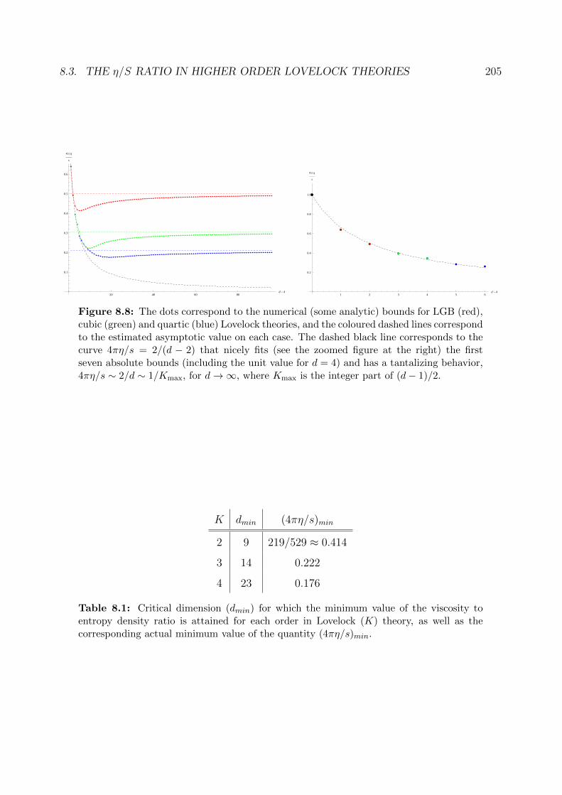
8.3. THE η/S RATIO IN HIGHER ORDER LOVELOCK THEORIES 205
20 40 60 80d - 4
0.1
0.2
0.3
0.4
0.5
0.6
4 Π Η
s
1 2 3 4 5 6d - 4
0.2
0.4
0.6
0.8
1.0
4 Π Η
s
Figure 8.8: The dots correspond to the numerical (some analytic) bounds for LGB (red),cubic (green) and quartic (blue) Lovelock theories, and the coloured dashed lines correspondto the estimated asymptotic value on each case. The dashed black line corresponds to thecurve 4πη/s = 2/(d − 2) that nicely fits (see the zoomed figure at the right) the firstseven absolute bounds (including the unit value for d = 4) and has a tantalizing behavior,4πη/s ∼ 2/d ∼ 1/Kmax, for d→∞, where Kmax is the integer part of (d− 1)/2.
K dmin (4πη/s)min
2 9 219/529 ≈ 0.414
3 14 0.222
4 23 0.176
Table 8.1: Critical dimension (dmin) for which the minimum value of the viscosity toentropy density ratio is attained for each order in Lovelock (K) theory, as well as thecorresponding actual minimum value of the quantity (4πη/s)min.
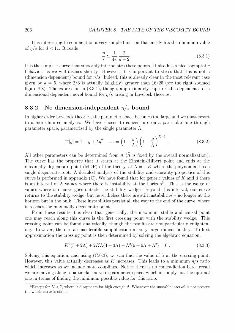
206 CHAPTER 8. THE FATE OF THE VISCOSITY BOUND
It is interesting to comment on a very simple function that nicely fits the minimum valueof η/s for d < 11. It reads
η
s' 1
4π
2
d− 2. (8.3.1)
It is the simplest curve that smoothly interpolates these points. It also has a nice asymptoticbehavior, as we will discuss shortly. However, it is important to stress that this is not a(dimension dependent) bound for η/s. Indeed, this is already clear in the most relevant casegiven by d = 5, where 2/3 is actually (slightly) greater than 16/25 (see the right zoomedfigure 8.8). The expression in (8.3.1), though, approximately captures the dependence of adimensional dependent novel bound for η/s arising in Lovelock theories.
8.3.2 No dimension-independent η/s bound
In higher order Lovelock theories, the parameter space becomes too large and we must resortto a more limited analysis. We have chosen to concentrate on a particular line throughparameter space, parametrized by the single parameter Λ:
Υ[g] = 1 + g + λg2 + . . . =(
1− g
Λ
)(1− g
Λ
)K−1
. (8.3.2)
All other parameters can be determined from Λ (Λ is fixed by the overall normalization).The curve has the property that it starts at the Einstein-Hilbert point and ends at themaximally degenerate point (MDP) of the theory, at Λ = −K where the polynomial has asingle degenerate root. A detailed analysis of the stability and causality properties of thiscurve is performed in appendix (C). We have found that for generic values of K and d thereis an interval of Λ values where there is instability at the horizon5. This is the range ofvalues where our curve goes outside the stability wedge. Beyond this interval, our curvereturns to the stability wedge, but nevertheless there are still instabilities – no longer at thehorizon but in the bulk. These instabilities persist all the way to the end of the curve, whereit reaches the maximally degenerate point.
From these results it is clear that generically, the maximum stable and causal pointone may reach along this curve is the first crossing point with the stability wedge. Thiscrossing point can be found analytically, though the results are not particularly enlighten-ing. However, there is a considerable simplification at very large dimensionality. To firstapproximation the crossing point is then determined by solving the algebraic equation,
K2(3 + 2Λ) + 2KΛ(4 + 3Λ) + Λ2(6 + 6Λ + Λ2) = 0 . (8.3.3)
Solving this equation, and using (C.0.3), we can find the value of λ at the crossing point.However, this value actually decreases as K increases. This leads to a minimum η/s ratiowhich increases as we include more couplings. Notice there is no contradiction here: recallwe are moving along a particular curve in parameter space, which is simply not the optimalone in terms of finding the minimum possible value for this ratio.
5Except for K < 7, where it disappears for high enough d. Whenever the unstable interval is not presentthe whole curve is stable.
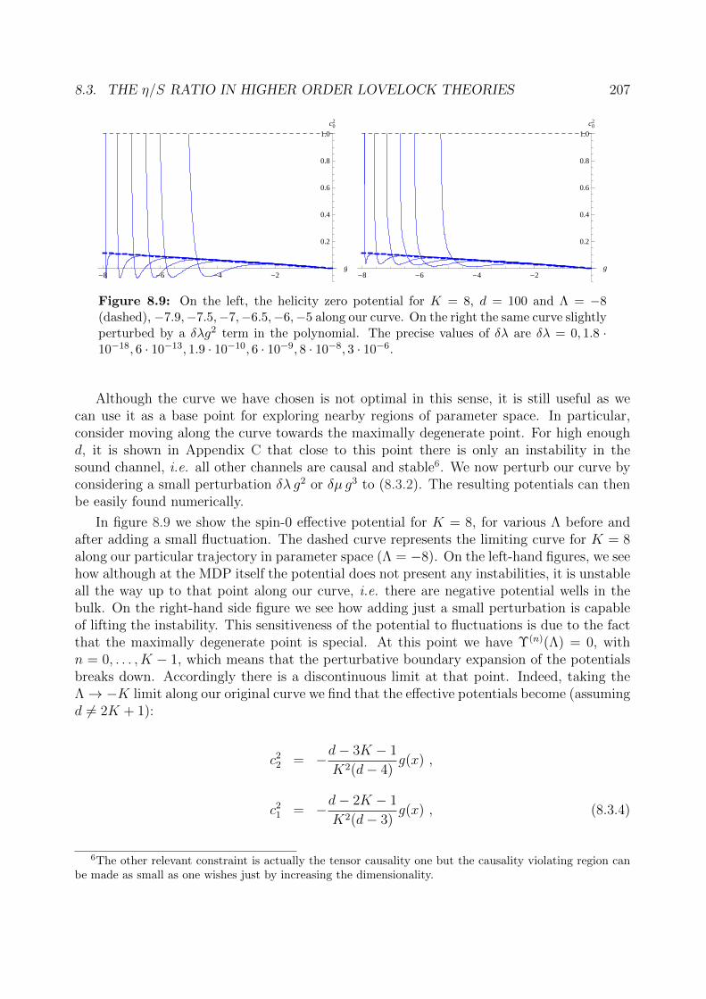
8.3. THE η/S RATIO IN HIGHER ORDER LOVELOCK THEORIES 207
-8 -6 -4 -2g
0.2
0.4
0.6
0.8
1.0
c02
-8 -6 -4 -2g
0.2
0.4
0.6
0.8
1.0
c02
Figure 8.9: On the left, the helicity zero potential for K = 8, d = 100 and Λ = −8(dashed), −7.9,−7.5,−7,−6.5,−6,−5 along our curve. On the right the same curve slightlyperturbed by a δλg2 term in the polynomial. The precise values of δλ are δλ = 0, 1.8 ·10−18, 6 · 10−13, 1.9 · 10−10, 6 · 10−9, 8 · 10−8, 3 · 10−6.
Although the curve we have chosen is not optimal in this sense, it is still useful as wecan use it as a base point for exploring nearby regions of parameter space. In particular,consider moving along the curve towards the maximally degenerate point. For high enoughd, it is shown in Appendix C that close to this point there is only an instability in thesound channel, i.e. all other channels are causal and stable6. We now perturb our curve byconsidering a small perturbation δλ g2 or δµ g3 to (8.3.2). The resulting potentials can thenbe easily found numerically.
In figure 8.9 we show the spin-0 effective potential for K = 8, for various Λ before andafter adding a small fluctuation. The dashed curve represents the limiting curve for K = 8along our particular trajectory in parameter space (Λ = −8). On the left-hand figures, we seehow although at the MDP itself the potential does not present any instabilities, it is unstableall the way up to that point along our curve, i.e. there are negative potential wells in thebulk. On the right-hand side figure we see how adding just a small perturbation is capableof lifting the instability. This sensitiveness of the potential to fluctuations is due to the factthat the maximally degenerate point is special. At this point we have Υ(n)(Λ) = 0, withn = 0, . . . , K − 1, which means that the perturbative boundary expansion of the potentialsbreaks down. Accordingly there is a discontinuous limit at that point. Indeed, taking theΛ→ −K limit along our original curve we find that the effective potentials become (assumingd 6= 2K + 1):
c22 = −d− 3K − 1
K2(d− 4)g(x) ,
c21 = −d− 2K − 1
K2(d− 3)g(x) , (8.3.4)
6The other relevant constraint is actually the tensor causality one but the causality violating region canbe made as small as one wishes just by increasing the dimensionality.
208 CHAPTER 8. THE FATE OF THE VISCOSITY BOUND
c20 = −d−K − 1
K2(d− 2)g(x) .
Since g(x) ∈ [Λ, 0] the above are actually always positive for sufficiently large dimensionality7.In particular, although the c0 potential always has a negative region for Λ larger than butclose to −K, it is actually tending discontinuously to a perfectly reasonable potential. Thisis clear from figure 8.9.
Our results then indicate that it is reasonable to expect that sufficiently close to the MDPthere should be a trajectory in parameter space which is both stable and causal. We haveshown this is certainly true up to K = 8. If this result holds for higher K, then it is alwayspossible to reach sufficiently close to the MDP and have well behaved effective potentials.As such, the theory seems to be well defined at that point.
At the MDP we have
λMDP =K − 1
2K(8.3.5)
and therefore a value of the viscosity to entropy ratio for very large dimensionality becomes(ηs
)MDP
=1
4π
1
K. (8.3.6)
By taking high enough K, this can be made arbitrarily small. Besides, since the maximumK, Kmax, is proportional to d/2 in the large d limit, we obtain the asymptotic behavioralready suggested by the formula (8.3.1) (see also figure 8.8).
To summarize, we have given evidence that it is possible to find a point in parameterspace, sufficiently close to the MDP of a particular Lovelock theory, such that no stabilityor causality issues occur for high enough d. In particular we have checked that it is possibleto do this up to K = 8. We conjecture that this can always be achieved for any K, and wetherefore come to the conclusion that the viscosity to entropy ratio can be made arbitrarilysmall by considering a Lovelock theory of high enough order. In other words, there is nobound for the η/s ratio which is independent of the dimensionality, at least in the class ofLovelock theories of gravity. This goes in line with our expectations that adding more andmore couplings, or free parameters in the lagrangian, it should be possible to reach lowerand lower values for the shear viscosity to entropy ratio.
It is interesting to mention at this point that the link between causality violation andthe viscosity bound does not apply for thermal theories undergoing a low temperature phasetransition. In [269] Buchel and Cremonini analyze this issue and made an important re-mark. The shear viscosity is one of the coupling coefficients of the effective hydrodynamicdescription of the theory. As such it applies to the regime of lowest momenta and frequency,i.e. ω, ‖k‖ << T , where the role of the temperature may also be played by by any othermicroscopic scale of the plasma – actually the smallest one. On exactly the opposite regime,microcausality is determined by the propagation of the high energy modes regime, i.e. , forω, ‖k‖ >> T . A link between both kinds of features is only possible if the same phase ofthe theory extends over the entire range of the energy scales. In other words, there must
7Remarkably the critical dimensionality, d > 3K + 1 is exactly the same found in chapter 4, required forarbitrarily small black holes to be stable.
8.4. DISCUSSION 209
not be any phase transitions in the plasma, as it happens for dual plasma of LGB gravity.As it is conformal just zero temperature phase transitions are allowed and we are always inthe deconfined high temperature phase. The only free parameter of the model is the LGBcoupling, which determines both the shear viscosity ratio and its causality properties. Hencethe link between the two is in a sense a mere coincidence. Any constraint on λ will translateinto an analogous restriction on η/s without any necessary deeper connection.
In the holographic setting UV and IR properties of the field theory correspond to geo-metrically distinct parts in AdS, the asymptotic and near-horizon regions respectively. Inthis sense it is clear that causality, found at the boundary, corresponds to the UV whereasstability, mostly related to the horizon, is a IR property. We have actually verified thatcausality plays a secondary role on the discussion of the possible bounds on η/s. Stabilityalone already prevents this ratio from becoming arbitrarily small at any fixed dimensionality,at least in the context of Lovelock gravities.
In the specific model of [269] the LGB term is sourced by the VEV of some irrelevantoperator that condensates in the IR below some critical temperature associated with thespontaneous breaking of some global U(1) symmetry. Geometrically, the broken phase ischaracterized by a scalar field with a non-trivial profile, vanishing at infinity but finite at thehorizon, the effective LGB coupling being proportional to that field. This effective couplingthus affects the value of the shear viscosity without changing the causality properties of theCFT. In a sense, we are lifting the causality restrictions but the stability ones are expectedto still hold. Stability still ensures the existence of a bound on η/s, a bound that reduces itsvalue as we increase the dimensionality and the order of the Lovelock theory accordingly.
8.4 Discussion
We have devoted this chapter to scrutinize the finite temperature phase of the CFT in thecontext of Lovelock theories. In particular we have considered in detail the restrictionsimposed by causality and stability on the shear viscosity to entropy ratio of the dual plasma.
An important part of our analysis was the study of these effective potentials, searchingfor causality violation or instabilities in the large momentum limit which might rule out re-gions of the parameter space. Notice, however, that while the former condition is a bona-fideconstraint on the theory, since it would lead to causality, the second seems to hold only forthe validity of the black brane solution, and is not a fundamental restriction. We have foundthat causality violation can occur deep inside the bulk, and therefore this effect cannot becaptured by a boundary expansion. This means that, contrary to previous expectations,causality violation is not necessarily a UV feature of the CFTs related to positivity of energyrestrictions8. Holographically this means that there are interesting constraints on the pa-rameters of the CFT which cannot be seen in perturbation theory. The field-theoretic originof such constraints remains a mystery.9 On the gravity side, these restrictions were essential
8§ Another example of this can be found in [10]. In that example we again recover the positivity constraintsfrom the asymptotic limit of a more general set.
9It would be of definite interest to study whether these constraints are related or not to unitarity restric-tions that were very recently shown to arise in the computation of 2-point functions of the stress-energytensor at finite temperature and large energy and momenta [39].
210 CHAPTER 8. THE FATE OF THE VISCOSITY BOUND
to prevent an arbitrarily small η/s ratio for a fixed theory, as seen for the concrete examplesof cubic and quartic Lovelock theories.
For higher order theories, we have resorted to the study of a particular curve throughparameter space. We chose this curve on the basis of simplicity and the capability of analytictreatment. The upshot of our analysis is that it seems likely that there is some curve leadingarbitrarily close to the maximally degenerate point of the theory. The reader might besuspicious about this – after all, at this point the central charge of the dual conformal fieldtheory is vanishing, and so is the kinetic term of the graviton fluctuations around the AdSblack hole. That is why we emphasize that one is really considering a curve leading to thispoint, but causality constraints keep us at a safe distance where everything is well defined.
In all cases we considered in detail, the minimum value for the ratio was obtained wellaway from the maximally degenerate point. In any case, we hope our work stimulates studyof the properties of the theory around this particular point. In the case d = 2K + 1,these theories display symmetry enhancement becoming gauge theories of the Chern-Simonsgroup: they have local AdS symmetry whereas all other theories with d > 2K + 1 havelocal Lorenz invariance [43]. Contrary to what is suggested by the fact that CT vanishesin the dual conformal field theory, there are some hints pointing towards the existence ofinteresting physics on these theories. For instance, the thermodynamics of their black holesdisplays a qualitative difference to that of generic AdS Lovelock black holes: the temperaturegrows linearly with the horizon radius, and the specific heat is a continuous, monotonicallyincreasing and positive function of r+ [164]. Thus, Chern-Simons black holes can reachthermal equilibrium with a heat bath at any temperature and they are stable under thermalfluctuations. There is also a mass gap between the massless black hole and AdS spacetime,as it happens in the case of d = 3 [270].
Our results indicate that, in the case of very large d, it should be possible to reach avalue of the η/s ratio of at least
η
s=
1
4π
1
K(8.4.1)
in the Kth order theory. Intuitively, this is simply telling us that the more parameters wehave, the lower the ratio can become. This is reminiscent of the species counter-argumentto a minimum bound on η/s [271,272]. Of course, in Lovelock gravity one needs to increasethe number of dimensions in order to have more parameters. Then it would seem thatfor all practical purposes there is a bound on η/s for any finite dimensionality. This iscertainly a possibility, and it is definitely true for Lovelock theory – a combination of stabilityand causality ensures it – even if we disregard the causality constraints a la Buchel andCremonini [269]. However, even for fixed dimensionality it seems that it might be possibleto have other interesting higher curvature corrections with finite coefficients [67–70]. Thesequasi-topological gravities have exact black hole solutions of a similar nature to those ofLovelock theory, including their thermodynamic features. However, hydrodynamic as wellas causality and stability properties, are quite different [71]. While there is much work tobe done understanding these theories, it seems plausible that the addition of high orderquasi-topological terms would lead to a smaller η/s ratio.
The stability wedge in all Lovelock theories has a non-trivial shape in the (λ,µ)-planebut is otherwise a cylinder in the remaining couplings. This means, in particular, that there
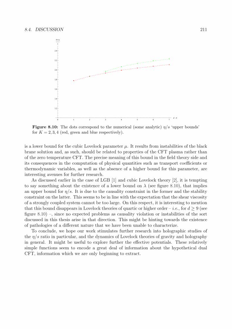
8.4. DISCUSSION 211
0 1 2 3 4 5 6 7d - 4
1.2
1.4
1.6
1.8
2.0
2.2
2.4
4 Π Η
s
Figure 8.10: The dots correspond to the numerical (some analytic) η/s ‘upper bounds’for K = 2, 3, 4 (red, green and blue respectively).
is a lower bound for the cubic Lovelock parameter µ. It results from instabilities of the blackbrane solution and, as such, should be related to properties of the CFT plasma rather thanof the zero temperature CFT. The precise meaning of this bound in the field theory side andits consequences in the computation of physical quantities such as transport coefficients orthermodynamic variables, as well as the absence of a higher bound for this parameter, areinteresting avenues for further research.
As discussed earlier in the case of LGB [1] and cubic Lovelock theory [2], it is temptingto say something about the existence of a lower bound on λ (see figure 8.10), that impliesan upper bound for η/s. It is due to the causality constraint in the former and the stabilityconstraint on the latter. This seems to be in line with the expectation that the shear viscosityof a strongly coupled system cannot be too large. On this respect, it is interesting to mentionthat this bound disappears in Lovelock theories of quartic or higher order – i.e., for d ≥ 9 (seefigure 8.10) –, since no expected problems as causality violation or instabilities of the sortdiscussed in this thesis arise in that direction. This might be hinting towards the existenceof pathologies of a different nature that we have been unable to characterize.
To conclude, we hope our work stimulates further research into holographic studies ofthe η/s ratio in particular, and the dynamics of Lovelock theories of gravity and holographyin general. It might be useful to explore further the effective potentials. These relativelysimple functions seem to encode a great deal of information about the hypothetical dualCFT, information which we are only beginning to extract.

212 CHAPTER 8. THE FATE OF THE VISCOSITY BOUND
Chapter 9
Summary and conclusions
“Who is more humble? The scientist who looksat the universe with an open mind
and accepts whatever the universe has to teach us,or somebody who says everything in this book
must be considered the literal truthand never mind the fallibility of all the human beings involved?”
Carl Sagan
Lovelock theory is the natural extension of general relativity to higher dimensions. It mayalso be thought of as a toy model for ghost-free higher curvature gravity. These gravity theo-ries capture some of the defining features of higher curvature gravities, namely the existenceof more than one (A)dS vacuum and intricate dynamics, more general black hole solutionsand instabilities; while avoiding some of their problems. In particular, Lovelock gravitiesyield second order field equations so that they can be considered beyond the perturbativeregime and are free of higher derivative ghosts. This provides an appealing arena to exploredifferent gravitational and holographic aspects of higher curvature gravity.
Most of the vacua of the theory support black holes that display interesting features.Besides, black holes with maximally symmetric horizons are subject to a version of Birkhoff’stheorem and these solutions can be found analytically. Most efforts in the literature havebeen devoted however to one particular branch of solutions, often restricted to a specificcombination of the Lovelock couplings. The branch usually chosen for the analysis is theso-called EH branch, as it actually reduces to the general relativistic solution as we turnoff the higher order couplings. In this thesis we have presented some tools that allow forthe description of Lovelock black holes for arbitrary values of the whole set of couplings,dimensionality and order of the theory. Despite the fact of the solution being implicit,
213
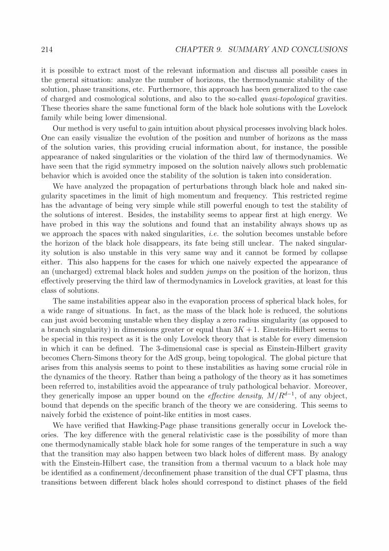
214 CHAPTER 9. SUMMARY AND CONCLUSIONS
it is possible to extract most of the relevant information and discuss all possible cases inthe general situation: analyze the number of horizons, the thermodynamic stability of thesolution, phase transitions, etc. Furthermore, this approach has been generalized to the caseof charged and cosmological solutions, and also to the so-called quasi-topological gravities.These theories share the same functional form of the black hole solutions with the Lovelockfamily while being lower dimensional.
Our method is very useful to gain intuition about physical processes involving black holes.One can easily visualize the evolution of the position and number of horizons as the massof the solution varies, this providing crucial information about, for instance, the possibleappearance of naked singularities or the violation of the third law of thermodynamics. Wehave seen that the rigid symmetry imposed on the solution naively allows such problematicbehavior which is avoided once the stability of the solution is taken into consideration.
We have analyzed the propagation of perturbations through black hole and naked sin-gularity spacetimes in the limit of high momentum and frequency. This restricted regimehas the advantage of being very simple while still powerful enough to test the stability ofthe solutions of interest. Besides, the instability seems to appear first at high energy. Wehave probed in this way the solutions and found that an instability always shows up aswe approach the spaces with naked singularities, i.e. the solution becomes unstable beforethe horizon of the black hole disappears, its fate being still unclear. The naked singular-ity solution is also unstable in this very same way and it cannot be formed by collapseeither. This also happens for the cases for which one naively expected the appearance ofan (uncharged) extremal black holes and sudden jumps on the position of the horizon, thuseffectively preserving the third law of thermodynamics in Lovelock gravities, at least for thisclass of solutions.
The same instabilities appear also in the evaporation process of spherical black holes, fora wide range of situations. In fact, as the mass of the black hole is reduced, the solutionscan just avoid becoming unstable when they display a zero radius singularity (as opposed toa branch singularity) in dimensions greater or equal than 3K + 1. Einstein-Hilbert seems tobe special in this respect as it is the only Lovelock theory that is stable for every dimensionin which it can be defined. The 3-dimensional case is special as Einstein-Hilbert gravitybecomes Chern-Simons theory for the AdS group, being topological. The global picture thatarises from this analysis seems to point to these instabilities as having some crucial role inthe dynamics of the theory. Rather than being a pathology of the theory as it has sometimesbeen referred to, instabilities avoid the appearance of truly pathological behavior. Moreover,they generically impose an upper bound on the effective density, M/Rd−1, of any object,bound that depends on the specific branch of the theory we are considering. This seems tonaively forbid the existence of point-like entities in most cases.
We have verified that Hawking-Page phase transitions generally occur in Lovelock the-ories. The key difference with the general relativistic case is the possibility of more thanone thermodynamically stable black hole for some ranges of the temperature in such a waythat the transition may also happen between two black holes of different mass. By analogywith the Einstein-Hilbert case, the transition from a thermal vacuum to a black hole maybe identified as a confinement/deconfinement phase transition of the dual CFT plasma, thustransitions between different black holes should correspond to distinct phases of the field
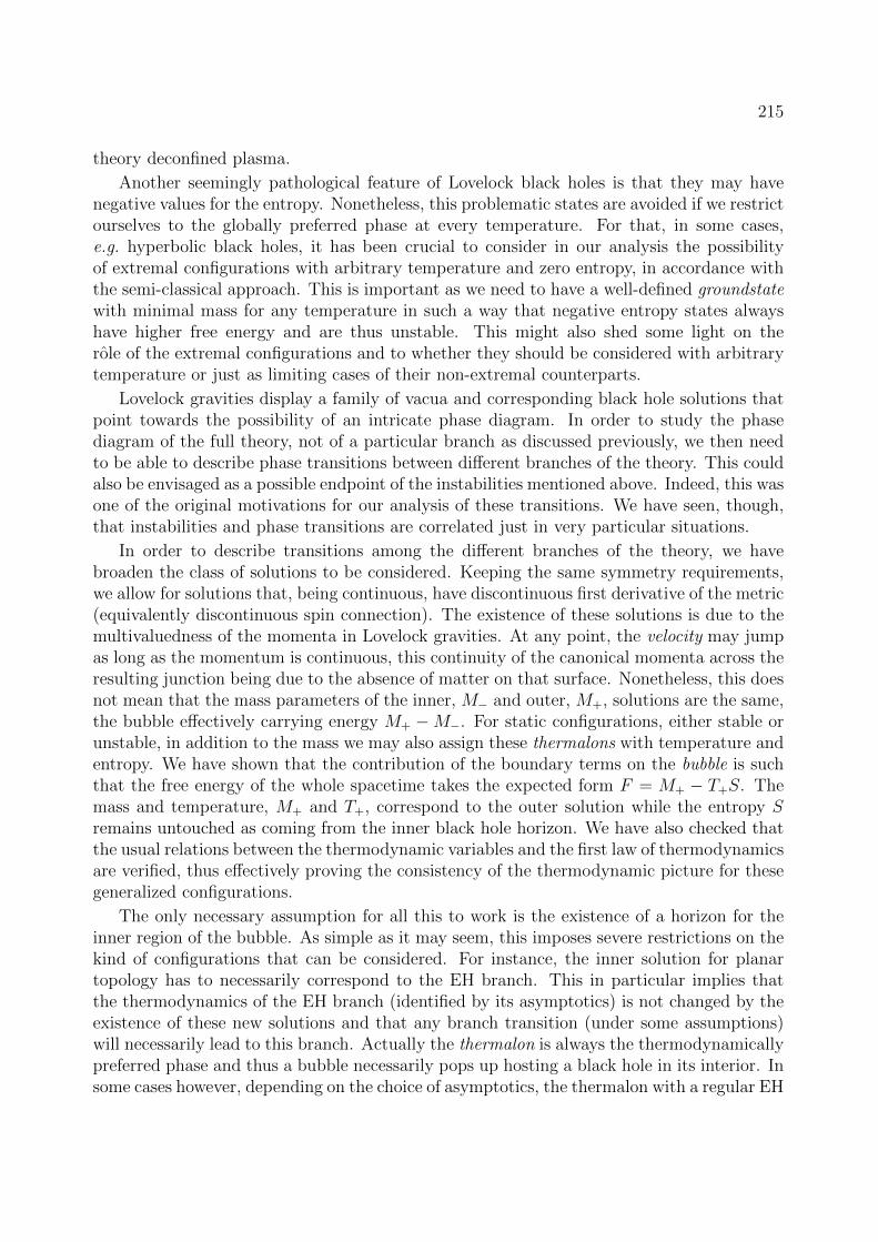
215
theory deconfined plasma.
Another seemingly pathological feature of Lovelock black holes is that they may havenegative values for the entropy. Nonetheless, this problematic states are avoided if we restrictourselves to the globally preferred phase at every temperature. For that, in some cases,e.g. hyperbolic black holes, it has been crucial to consider in our analysis the possibilityof extremal configurations with arbitrary temperature and zero entropy, in accordance withthe semi-classical approach. This is important as we need to have a well-defined groundstatewith minimal mass for any temperature in such a way that negative entropy states alwayshave higher free energy and are thus unstable. This might also shed some light on therole of the extremal configurations and to whether they should be considered with arbitrarytemperature or just as limiting cases of their non-extremal counterparts.
Lovelock gravities display a family of vacua and corresponding black hole solutions thatpoint towards the possibility of an intricate phase diagram. In order to study the phasediagram of the full theory, not of a particular branch as discussed previously, we then needto be able to describe phase transitions between different branches of the theory. This couldalso be envisaged as a possible endpoint of the instabilities mentioned above. Indeed, this wasone of the original motivations for our analysis of these transitions. We have seen, though,that instabilities and phase transitions are correlated just in very particular situations.
In order to describe transitions among the different branches of the theory, we havebroaden the class of solutions to be considered. Keeping the same symmetry requirements,we allow for solutions that, being continuous, have discontinuous first derivative of the metric(equivalently discontinuous spin connection). The existence of these solutions is due to themultivaluedness of the momenta in Lovelock gravities. At any point, the velocity may jumpas long as the momentum is continuous, this continuity of the canonical momenta across theresulting junction being due to the absence of matter on that surface. Nonetheless, this doesnot mean that the mass parameters of the inner, M− and outer, M+, solutions are the same,the bubble effectively carrying energy M+ −M−. For static configurations, either stable orunstable, in addition to the mass we may also assign these thermalons with temperature andentropy. We have shown that the contribution of the boundary terms on the bubble is suchthat the free energy of the whole spacetime takes the expected form F = M+ − T+S. Themass and temperature, M+ and T+, correspond to the outer solution while the entropy Sremains untouched as coming from the inner black hole horizon. We have also checked thatthe usual relations between the thermodynamic variables and the first law of thermodynamicsare verified, thus effectively proving the consistency of the thermodynamic picture for thesegeneralized configurations.
The only necessary assumption for all this to work is the existence of a horizon for theinner region of the bubble. As simple as it may seem, this imposes severe restrictions on thekind of configurations that can be considered. For instance, the inner solution for planartopology has to necessarily correspond to the EH branch. This in particular implies thatthe thermodynamics of the EH branch (identified by its asymptotics) is not changed by theexistence of these new solutions and that any branch transition (under some assumptions)will necessarily lead to this branch. Actually the thermalon is always the thermodynamicallypreferred phase and thus a bubble necessarily pops up hosting a black hole in its interior. Insome cases however, depending on the choice of asymptotics, the thermalon with a regular EH
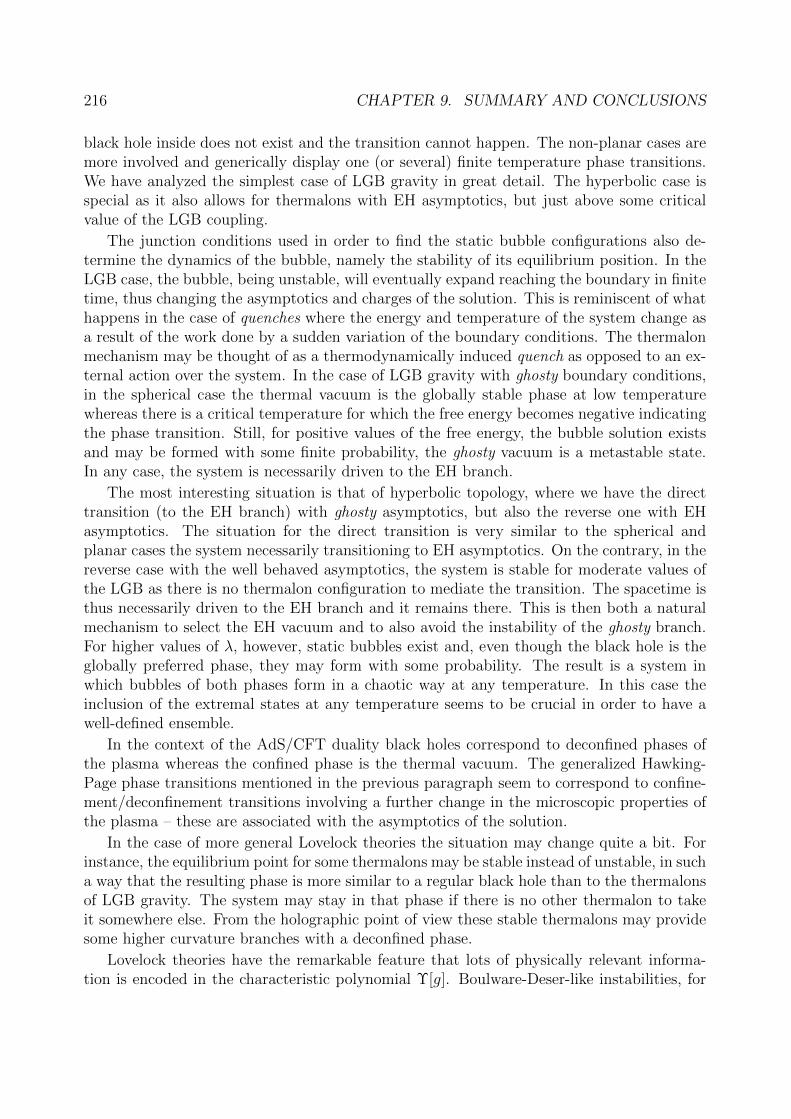
216 CHAPTER 9. SUMMARY AND CONCLUSIONS
black hole inside does not exist and the transition cannot happen. The non-planar cases aremore involved and generically display one (or several) finite temperature phase transitions.We have analyzed the simplest case of LGB gravity in great detail. The hyperbolic case isspecial as it also allows for thermalons with EH asymptotics, but just above some criticalvalue of the LGB coupling.
The junction conditions used in order to find the static bubble configurations also de-termine the dynamics of the bubble, namely the stability of its equilibrium position. In theLGB case, the bubble, being unstable, will eventually expand reaching the boundary in finitetime, thus changing the asymptotics and charges of the solution. This is reminiscent of whathappens in the case of quenches where the energy and temperature of the system change asa result of the work done by a sudden variation of the boundary conditions. The thermalonmechanism may be thought of as a thermodynamically induced quench as opposed to an ex-ternal action over the system. In the case of LGB gravity with ghosty boundary conditions,in the spherical case the thermal vacuum is the globally stable phase at low temperaturewhereas there is a critical temperature for which the free energy becomes negative indicatingthe phase transition. Still, for positive values of the free energy, the bubble solution existsand may be formed with some finite probability, the ghosty vacuum is a metastable state.In any case, the system is necessarily driven to the EH branch.
The most interesting situation is that of hyperbolic topology, where we have the directtransition (to the EH branch) with ghosty asymptotics, but also the reverse one with EHasymptotics. The situation for the direct transition is very similar to the spherical andplanar cases the system necessarily transitioning to EH asymptotics. On the contrary, in thereverse case with the well behaved asymptotics, the system is stable for moderate values ofthe LGB as there is no thermalon configuration to mediate the transition. The spacetime isthus necessarily driven to the EH branch and it remains there. This is then both a naturalmechanism to select the EH vacuum and to also avoid the instability of the ghosty branch.For higher values of λ, however, static bubbles exist and, even though the black hole is theglobally preferred phase, they may form with some probability. The result is a system inwhich bubbles of both phases form in a chaotic way at any temperature. In this case theinclusion of the extremal states at any temperature seems to be crucial in order to have awell-defined ensemble.
In the context of the AdS/CFT duality black holes correspond to deconfined phases ofthe plasma whereas the confined phase is the thermal vacuum. The generalized Hawking-Page phase transitions mentioned in the previous paragraph seem to correspond to confine-ment/deconfinement transitions involving a further change in the microscopic properties ofthe plasma – these are associated with the asymptotics of the solution.
In the case of more general Lovelock theories the situation may change quite a bit. Forinstance, the equilibrium point for some thermalons may be stable instead of unstable, in sucha way that the resulting phase is more similar to a regular black hole than to the thermalonsof LGB gravity. The system may stay in that phase if there is no other thermalon to takeit somewhere else. From the holographic point of view these stable thermalons may providesome higher curvature branches with a deconfined phase.
Lovelock theories have the remarkable feature that lots of physically relevant informa-tion is encoded in the characteristic polynomial Υ[g]. Boulware-Deser-like instabilities, for
217
instance, can be simply written as Υ′[Λ] < 0, which has a beautiful CFT counterpart tellingus that the central charge, CT , has to be positive. We have computed the central charge CT ,making the above statement concrete, as well as the two extra parameters, t2 and t4, involvedin 3-point functions of the stress-energy tensor. t4 is actually vanishing for the particularcase of Lovelock theories. This might be related to some kind of supersymmetry constrainton the dual CFT, although the supersymmetric version of general Lovelock theories is un-known. We have also discussed the possible terms that may contribute to the computationof t2 and t4 in the context of general higher curvature gravity. Restricting to terms yielding2-derivative equations of motion in the shock wave background, there is a one-to-one corre-spondence between the possible structures appearing in the energy flux 1-point function andthe contributions from higher curvature terms. This is also consistent with the number offield redefinition invariant combinations that can be written in the action.
Another very interesting correspondence that has been observed using Lovelock theoryis the one that relates holographic causality in the bulk of AdS with positivity of the energyflux expectation values. Both physical requirements are very different in nature, yet theyimply the same set of constraints on t2 (for t4 = 0). Lacking a definitive proof of thepositivity of energy fluxes, this may also be considered as indirect evidence in the restrictedcontext of Lovelock holography. Moreover, this has led to the discovery of these conditionsbeing required by unitarity of the corresponding CFT [39]. Furthermore, even though theconnection was first found for the case of black hole backgrounds, this is not a featureof thermal CFTs. We have in fact performed a similar computation using a shock wavebackground and found a complete agreement with the previous sets of constraints. Thissecond computation is also simpler in the sense that it makes clear that the problem arisesfrom the 3-graviton vertex. Notice that, contrary to the instabilities found before, causalityviolation is a bona fide pathology and it should be discarded as unphysical. The instabilities,in turn, might just be pointing to the existence of new solutions or to other issues such asnot being expanding about the true vacuum. In the case of Lovelock gravity stability is justnecessary for the validity of the black hole solution and is not a fundamental restriction.
The above physical constraints restrict the possible values of the Lovelock couplingsthat describe a causal CFT with positive energy fluxes. Notice that this connection couldhave never been discovered in the perturbative regime as we need t2 or t4 of order onefor the theory to ever violate causality. Besides, in the supergravity approximation, t2 ∼α′. All this, and the fact that all formulæ seem to extend meaningfully and smoothlyto arbitrary dimension and order of Lovelock gravity, seem to entail the applicability ofthe AdS/CFT correspondence beyond the context of critical string theory. Although thesimplest Lovelock invariant has appeared in the context of string realizations of the duality,higher order Lovelock terms do not show up in that context, nor higher curvature correctionswith finite coefficients. Do strongly coupled CFTs necessarily have equal central changes infour dimensions? The answer to this question does not seem to be easy and we have notfound any hint pointing in any clear direction.
When dealing with higher order Lovelock gravities, contrary to previous expectations wehave also found causality violation far from the boundary of the spacetime, thus showing thatthis particular pathology is not necessarily linked to the UV properties of the field theory,neither to positivity of the energy flux expectation values alone. It would be interesting to
218 CHAPTER 9. SUMMARY AND CONCLUSIONS
study if this effect could be traced back to positivity of energy flux higher point functions.
Finally, we have analyzed the constraints imposed by causality/positivity to other rel-evant quantities of the CFT, namely transport coefficients such as the shear viscosity toentropy density ratio. This ratio gets corrected from the universal KSS value η/s = 1/4π bythe LGB coupling in such a way that any positive value of λ would entail a violation of thecelebrated bound. Besides, an upper bound on λ automatically translates into a lower boundin η/s. Even though higher order Lovelock terms do not appear explicitly in the correctedexpression for η/s, they actually affect the value of the bound. They add some freedom thatconsequently allows λ to take higher values, thus lowering the bound. We have discussed theexistence of a bound in that context and realized that causality alone cannot prevent theratio to take arbitrarily low values, even negative in some cases. Besides, one can constructeffective holographic models where the LGB term is sourced by a VEV of another field thatcondenses in the IR, i.e. it has a finite value just close to the horizon being zero asymptoti-cally. In this way, the addition of the LGB correction does not affect the asymptotic causalproperties of the theory while changing the value of the shear viscosity. In a sense we canlift in this manner the causality restriction on η/s.
The restrictions that avoid unphysical values of the shear viscosity arise once again fromstability. After all, negative shear viscosity also corresponds to an instability of the system.Using the stability analysis in the high momentum regime, we have shown that a nonzerobound on the shear viscosity to entropy density actually exists for any dimensionality d, theminimum value of η/s approaching zero as we go to higher and higher dimensions. Ourresults indicate that for very large d it should be possible to reach a value of 4πη/s of atleast 1/K. Up to ten dimensions (i.e. quartic order) it can be shown that the lowest boundfor each dimensions roughly follows a curve given by 4πη/s ≈ 1/(d− 2).
Along this thesis I have tried to present Lovelock theories as an interesting playgroundfor testing our ideas about gravity and the holographic duality. This provided interestinginformation about viable modifications of Einstein-Hilbert gravity and, by contrast, alsoshed some light on general relativity in four or higher dimensions. Lovelock gravities havemany interesting features, a rich dynamics and effects that cannot be observed in thatsimpler case. This would also allow us to look at Einstein-Hilbert gravity under new light,putting it in a much broader context and maybe understanding what is so special aboutit. Our investigations led to deep connections between seemingly unrelated concepts. Theseunsuspected insights have the most celebrated instance in the exact equivalence betweencausality in AdS and positivity of the energy in the CFT, but we have uncovered more subtleexamples. Instabilities play a central role in this context being related to the preservationof the cosmic censorship hypothesis and the third law of black hole mechanics in Lovelockgravity. Stability seems to be relevant for the evaporation process of black holes as well, andfor the existence of a bound for η/s. The diversity of situations for which instabilities appearto have a relevant role is quite vast and deserves further investigation. Also, it would beinteresting to analyze further implications of them in the context of AdS/CFT, particularlyon the possible values of other transport coefficients of the dual plasma.
After this long journey, Lovelock theories emerge as a complex and interesting set oftheories, consistent as far as we can tell. Still, there are plenty of open avenues for furtherresearch, many unresolved issues. In higher dimensions there is a enormous increase in the
219
variety of rotating solutions, black rings, black saturns, multi black rings, etc. One interestingquestion to be answered in the context of Lovelock gravity would be to what extent this richstructure survives. There is a long way to go though as we do not even know the exactform of the simplest rotating solutions. Another insufficiently explored issue is that of thedimensional reduction of Lovelock theories, the relations under compactification betweentheories of different order – namely with Einstein-Hilbert gravity – and the stimulatingpossibility of these theories undergoing self-driven compactification. In exploring ways tosimplify and get further insight into the dynamics of gravity, some attention has been recentlydrawn to the large d limit of gravity. Lovelock gravity provide the most obvious extensionalso in this respect as they offer a second parameter K, the order of the theory, that can scaleas fast as the dimension. In the holographic context the notion of entanglement entropy hasalso recently attracted a lot of attention and Lovelock gravity seem to be a suitable testbedin that case as well. Finally, as it was already mentioned in the main text, Lovelock theories,through the AdS/CFT correspondence, open a window into the realm of higher dimensionalCFTs, which we do not know much about.
We hope that the tools and information obtained through our analysis will be valuablefor tackling these and other interesting questions, also when dealing with higher curvaturecorrections of generic type.

220 CHAPTER 9. SUMMARY AND CONCLUSIONS
Appendix A
Master equations for highmomentum perturbations
A.1 Black hole perturbations
We shall consider perturbations of the metric around the black hole solution obtained in theprevious sections along a given direction parallel to the boundary (say, xd−1 ≡ z) and propa-gating towards the interior of the geometry. Using the direction z as an axis of symmetry, wecan classify the perturbations in helicity representations of the rotation group around it. Itis convenient to analyze each case separately. The linear order contribution to the equationsof motion (1.1.5) can be written as
δEa = εaf1···fd−1
[ d−12
]∑k=0
ck[k δRf1f2 ∧Rf3···f2k ∧ ef2k+1···fd−1
+ (d− 2k − 1)Rf1···f2k ∧ ef2k+1···fd−2 ∧ δefd−1]
= 0 . (A.1.1)
Helicity two perturbation
The easiest case is the one with higher helicity. For symmetry reasons we can choosethe helicity two perturbation, hµν(t, r, z)dxµdxν , simply as1 h23(t, r, z) dx2dx3. Since wewill consider small perturbations, it is convenient to include an infinitesimal parameter ε,
1In principle, one should consider hij , with i < j = 2, . . . , 6, but their equations are all decoupled andgive rise to the same answer. The remaining helicity two components are hii − hjj , with i, j = 2, . . . , 6, butsince diagonal components can be made all equal by rotation, hii = 0.
221
222 APPENDIX A. MASTER EQUATIONS
h23(t, r, z) = ε φ(t, r, z). This can be readily included in the vielbein as ea = ea + ε δea [1],
e 0 =√f dt , e1 =
1√fdr , eF =
r
LdxF , F=4...d−1 ,
e2 =r
L
(1 +
ε
2φ) (dx2 + dx3
), e3 =
r
L
(1− ε
2φ) (dx2 − dx3
). (A.1.2)
From the torsionless condition we can now calculate the first order corrections to the spin-connection, ωab = ωab + ε δωab, and from them those to the curvature 2-form,
δRab = d(δωab) + δωac ∧ ωcb + ωac ∧ δωcb . (A.1.3)
Consider now the Fourier transform of the perturbation,
φ(t, r, z) =
∫dω
2π
dq
2πφ(r; k) e−iωt+iqz , k = (ω, 0, . . . , 0, q) . (A.1.4)
For the sake of clarity, we omit the k dependence in φ in what follows.The first thing we have to realize in order to carry out this calculation is that the relevant
contributions to order ω2, q2 and ω q, come from derivatives along the directions e0 and ed−1.In the simplest case, for helicity two perturbations, these contributions have only an effect onthe expressions of δω02, δω03, δω(d−1)2 and δω(d−1)3. Since we are at the linearized level, weconclude that the only non-trivial contributions to order ω2, q2, ω q come from their exteriorderivative (the second term in (A.1.1) is also irrelevant),
δR02 ≈ d(δω02) = −ω2
2fφ e0 ∧ e2 +
ω qL
2r√fφ ed−1 ∧ e2 , (A.1.5)
δR(d−1)2 ≈ d(δω(d−1)2) = −q2L2
2r2φ ed−1 ∧ e2 − ω qL
2r√fφ e0 ∧ e2 , (A.1.6)
where the symbol ≈ refers to those contributions relevant to compute the propagation speedof a boundary perturbation. There are analogue expressions (with the opposite sign) for thecomponents with a leg along the e3 direction. Notice that the cosmological constant term isirrelevant for our purposes.
Recalling from (2.1.6) that the curvature 2-form of the black-hole spacetime is propor-tional to ea ∧ eb, it is immediate to see that the only non-vanishing contributions are thosewith d(δωab) behaving equally,
d(δω02) ≈ −ω2
2fφ e0 ∧ e2 , d(δω(d−1)2) ≈ −q
2L2
2r2φ ed−1 ∧ e2 , (A.1.7)
(and, of course, an analogous expression for d(δω03) and d(δω(d−1)3)). Some of the equations
of motion are trivially satisfied. Indeed, notice that δE (d)a ≈ 0 trivially, unless a = 2 or 3.
This is due to cancellations of contributions coming from d(δω02) and d(δω03) (similarly,d(δω(d−1)2) and d(δω(d−1)3)). Moreover, by symmetry, the two non-trivial equations just
A.1. BLACK HOLE PERTURBATIONS 223
differ by a global sign. We must then focus on a single component of (A.1.1), say, δE (d)3 = 0.
The contribution to first order from each Lovelock term can be written as
δE (d)3 = 2
ε302f3···fd−1
[ d−12
]∑k=1
k ck d(δω02) ∧Rf3···f2k ∧ ef2k+1···fd−1
+ ε3(d−1)2f3···fd−1
[ d−12
]∑k=1
k ck d(δω(d−1)2) ∧Rf3···f2k ∧ ef2k+1···fd−1
= 0 . (A.1.8)
To proceed, the only thing to worry about is where the 0 and 1 indices are, since dependingon them the curvature 2-form components change (2.1.6). Notice that the first (second) linegives the ω2 (q2) contribution. The former, for instance, can be nicely rewritten in terms ofg(r),
δE3, ω = −ω2
fφ
K∑k=0
k ck(r(gk−1)′ + (d− 3)gk−1
)(d− 4)! , (A.1.9)
while the latter reads
δE3, q =q2L2
r2φ
K∑k=0
k ck(r2(gk−1)′′
+ 2(d− 3)r(gk−1)′ + (d− 3)(d− 4)gk−1)
(d− 5)! . (A.1.10)
Here we assume that ck>K = 0. It is convenient to define the following functionals, C(k)d [f, r],
involving up to kth-order derivatives of f (or g):
C(0)d [g, r] = Υ′[g] , (A.1.11)
C(1)d [g, r] =
(rd
dr+ (d− 3)
)Υ′[g] , (A.1.12)
C(2)d [g, r] =
(rd
dr+ (d− 3)
)(rd
dr+ (d− 4)
)Υ′[g] . (A.1.13)
Then, the speed of the helicity two graviton can be written as (see [1] for details)
c22(r) ≡ q2
ω2=
L2f
(d− 4)r2
C(2)d [g, r]
C(1)d [g, r]
, (A.1.14)
Helicity one perturbation
It is a bit more involved but the same can be done for the other polarizations. In order tochoose an helicity one perturbation, we can proceed with a gauge fixing (h0a = 0) and, bysymmetry arguments, just turn on the components h12(t, r, z) = ε φ(t, r, z) and h26(t, r, z) =
224 APPENDIX A. MASTER EQUATIONS
ε ψ(t, r, z) (recall that the direction 1 is the radial one and d− 1 is the propagation z). Theperturbation, thus, can be parametrized as,
e 0 =√f dt , e1 =
1√fdr +
r
Lε φ dx2 ,
e2 =r
L
(dx2 + ε ψdz
), eB =
r
LdxB , B=3,4,...d−1 . (A.1.15)
Proceeding as in the previous case we get a set of algebraic equations that sets one of thecomponents, h2(d−1), to zero. The remaining equation yields directly the speed of the gravitonas in the previous case
c21 =
L2f
(d− 3) r2
C(1)d [g, r]
C(0)d [g, r]
. (A.1.16)
Helicity zero perturbation
We can proceed in the same way as we did for the other two types of perturbations. Thehelicity zero perturbation is, anyway, a bit more involved. After gauge fixing, we still needto turn on several components h11 = ψ(t, r, z), h22 = h33 = h44 = h55 = ξ(t, r, z), h16 =φ(t, r, z), and h66 = ϕ(t, r, z) (as before, we will call their Fourier transforms respectivelyψ(r), ξ(r), φ(r) and ϕ(r). The vielbein for this case reads,
e 0 =√f dt , e1 =
1√f
(1 +
ε
2ψ)dr +
r
Lε φ dz , (A.1.17)
ed−1 =r
L
(1 +
ε
2ϕ)dz , eB =
r
L
(1 +
ε
2ξ)dxB , B=2,3,...d−2 . (A.1.18)
One of the components, φ, is set to zero by the equations of motion, while other two can bewritten in terms of only one degree of freedom
ψ = −C(1)d [g, r]
C(0)d [g, r]
ξ , ϕ =
(q2
ω2
L2f(r)
r2
C(1)d [g, r]
C(0)d [g, r]
− (d− 3)
)ξ . (A.1.19)
When we substitute these expressions into the equations of motion, only one of them remainslinearly independent and gives the speed of the helicity zero graviton
c20 =
L2f
(d− 2) r2
(2 C(1)
d [f, r]
C(0)d [f, r]
− C(2)d [f, r]
C(1)d [f, r]
). (A.1.20)
The above expressions are valid for arbitrary higher order Lovelock theory and higher di-mensional spacetimes. Instead of analyzing these expressions right away, let us discuss analternative computation, first introduced in [237], given by the scattering of gravitons andshock waves.
A.2. SHOCK WAVES AND GRAVITONS 225
A.2 Shock waves and gravitons
It is more convenient to work in Poincare coordinates, z = 1/r. We insist in performing allcomputations in the formalism used in the previous section since it is significantly simplerthan the usual tensorial setup. We define light-cone coordinates2 u = t+ x6 and v = t− x6,and consider a shock wave propagating on AdS along the radial direction,
ds2AdS,sw = ds2
AdS + f(u)$(xa, z) du2 . (A.2.1)
We should think of f(u) as a distribution with support in u = 0, which we will finally identifyas a Dirac delta function. As we did in the previous section, we consider an helicity twograviton perturbation, h23 dx
2dx3, which we keep infinitesimal h23 = ε φ,
ds2AdS,sw =
N2#
L2
−dudv + dxidxi + 2εφ dx2dx3 + L4dz2
z2+ f(u)$(xa, z) du2 . (A.2.2)
The calculation is very similar to the one in the previous section. We just have to modifythe vielbein considered as the input. In this case,
e 0 =N#
Lzdu , e1 =
N#
Lzdv − Lz
N#
f(u)$(xa, z) du ,
e2 =N#√2Lz
(1 +
ε
2φ)
(dx2 + dx3) , e3 =N#√2Lz
(1− ε
2φ)
(dx2 − dx3) ,
eK =N#
LzdxK , K=4,5,...d−2 , ed−1 =
N#L
zdz . (A.2.3)
The constant N# (7.1.3) is related to the radius of the AdS space, and the perturbationdepends only on (u, v, z) as before. The shock wave is parametrized by the function $(xa, z).
Introducing (A.2.3) into the equations of motion for the background (ε → 0) we get anequation for N# yielding the already known possible values, and the equation for the shockwave propagating on AdS (6.2.22). There are several possible solutions for this equation.The one we are going to consider is
$ = αN2# z
d−3 , (A.2.4)
which, as discussed in [237], can be obtained from the black hole background by boostingthe solution while keeping its energy constant. The normalization constant α is proportionalto the energy density and, as such, must be positive if the solution has a positive mass.
For perturbations propagating on top of these backgrounds, the procedure is almost thesame as in the previous section, just a bit more complicated since the symmetry of thebackground is lower than in the black hole solution. As before, since we are only interestedin the high momentum limit, we keep only contributions of the sort ∂2
vφ, ∂u∂vφ and ∂2uφ.
2We then have to change the tangent space metric to η00 = η11 = 0, η01 = η10 = − 12 , ηAB =
diag(1, 1, · · · , 1),A,B=2,...,6.
226 APPENDIX A. MASTER EQUATIONS
These contributions come again from the exterior derivative of the perturbation of the spinconnection. In the helicity two case
d(δω02) =L2 z2
N2#
[∂2vφ e
1 ∧ e2 +(∂u∂vφ+ αf(u)L2zd−1 ∂2
vφ)e0 ∧ e2
], (A.2.5)
d(δω12) =L2 z2
N2#
[(∂u∂vφ+ αf(u)L2zd−1 ∂2
vφ)e1 ∧ e2 + (· · · ) e0 ∧ e2
], (A.2.6)
the ellipsis being used in the second expression since the corresponding term does not con-tribute to the equations of motion. The components with index 3 instead of 2 are the onlyremaining ones non-vanishing, and they are obtained changing φ→ −φ. The other thing weneed is the curvature 2-form of the background metric, that can be written as
Rab = Λ(ea ∧ eb +Xab) , (A.2.7)
where Λ = − 1L2N2
#and Xab is an antisymmetric 2-form accounting for the contribution of
the shock wave
X1a = (d− 1)α f(u)L2 zd−1 e0 ∧ ea , a 6= 0, d− 1 ,
X1(d−1) = −[(d− 2)2 − 1]α f(u)L2 zd−1 e0 ∧ ed−1 .
Now, the relevant equation is, as before, given by a single component of (A.1.1),
δE3 =K∑k=1
k ck ε3f1···fd−1d(δωf1f2) ∧Rf3···f2k ∧ ef2k+1··· fd−1
= 2K∑k=1
k ck[ε302f3···fd−1
d(δω02) + ε312f3···fd−1d(δω12)
]∧Rf3···f2k ∧ ef2k+1··· fd−1
=4L2z2
N2#
K∑k=1
k ck Λk−1[(d− 3)!
(∂u∂vφ+ αf(u)L2zd−1∂2
vφ)− (k − 1)×
×(d− 5)!((d− 5)(d− 1)− [(d− 2)2 − 1]
)αf(u)L2zd−1∂2
vφ]dV ol , (A.2.8)
since the diagonal part of d(δωab) contributes to all the diagonal parts of Rab and the off-diagonal part of d(δωab) contributes to the off-diagonal part of one of the Rab. Collectingterms type ∂u∂vφ and ∂2
vφ and simplifying constant factors (not depending on the degree ofthe Lovelock term, k), δE3 = 0 implies
Υ′[Λ]
[∂u∂vφ+
(1 +
2(d− 1)ΛΥ′′[Λ]
(d− 3)(d− 4)Υ′[Λ]
)αf(u)L2zd−1∂2
vφ
]= 0 . (A.2.9)
As it should be expected we get Υ′[Λ] as an overall constant related to the unitarity propertiesof these perturbations and the constant factor multiplying the ∂2
vφ term can be written interms of t2 defined in (6.2.29) as
N2 = 1 +2(d− 1)ΛΥ′′[Λ]
(d− 3)(d− 4)Υ′[Λ]= 1− 1
d− 2t2 (A.2.10)
A.2. SHOCK WAVES AND GRAVITONS 227
The equations of motion for the other two helicities have exactly the same form with
N1 = 1 +d− 4
2(d− 2)t2 ; N0 = 1 +
d− 4
d− 2t2 (A.2.11)
As discussed in chapter 7 this equations will be relevant when discussing holographic causalityproperties of this spacetimes in the context of the AdS/CFT correspondence.

228 APPENDIX A. MASTER EQUATIONS
Appendix B
3-point function parameters
Conformal symmetry is powerful enough to determine the form of the 3-point function forthe stress-energy tensor up to five constants and this are further constrained by conservationlaws allowing us to reduce the number of independent parameters to three, A, B and C.Further one finds that Ward identities relate the 2- and 3-point functions and so CT can beexpressed in terms of these three constants.
CT =Ωd−2
2
(d− 2)(d+ 1)A− 2B − 4dC(d− 1)(d+ 1)
(B.0.1)
where Ωd−2 is the area of the unit (d− 2)-sphere. Also as the energy flux 1-point function isjust a quotient of a 3- and a 2-point function t2 and t4 should also be writeable in terms ofthe three parameters A, B and C. This was done in [37] yielding
t2 =2d
d− 1
(d− 3)(d+ 1)dA+ 3(d− 1)2B − 4(d− 1)(2d− 1)C(d− 2)(d+ 1)A− 2B − 4dC
,
t4 = − d
d− 1
(d+ 1)(2(d− 1)2 − 3(d− 1)− 3)A+ 2(d− 1)2(d+ 1)B − 4(d− 1)d(d+ 1)C(d− 2)(d+ 1)A− 2B − 4dC
,
Then the scalar, vector and tensor constraints coming from from the positivity of energy canalso be translated into
− d
d− 1
(d− 3)(d+ 1)A+ 2(d− 1)B − 4(d− 1)C(d− 2)(d+ 1)A− 2B − 4dC
≥ 0 ,
d(d− 3)(d+ 1)A+ (3d− 5)B − 8(d− 1)C
(d− 2)(d+ 1)A− 2B − 4dC≥ 0 , (B.0.2)
−2d2(d− 2)B − 2C
(d− 2)(d+ 1)A− 2B − 4dC≥ 0 .
constraints that can be identified with those coming from causality in the boundary theoryin order to obtain expressions for A,B, C. However in order to unambiguously determine the
229
230 APPENDIX B. 3-POINT FUNCTION PARAMETERS
normalization of these coefficients we can just obtain them in terms of CT , t2, t4 and plugthe expressions for these into them. We obtain then
A = −(d− 1)3
(d− 2)3
Γ[d]
πd−1
1
(−Λ)d/2
(2dΛΥ′′[Λ]
(d− 4)2+ Υ′[Λ]
),
B = − (d− 1)
(d− 2)3
Γ[d]
πd−1
1
(−Λ)d/2
((d− 1)d (d2 − 4d+ 6) ΛΥ′′[Λ]
(d− 4)2+(d3 − 4d2 + 5d− 1
)Υ′[Λ]
),
C = − (d− 1)2
2(d− 2)3
Γ[d]
πd−1
1
(−Λ)d/2
((d3 − 3d2 + 3d− 4) ΛΥ′′[Λ]
(d− 4)2+
1
2(2(d− 3)d+ 3)Υ′[Λ]
).
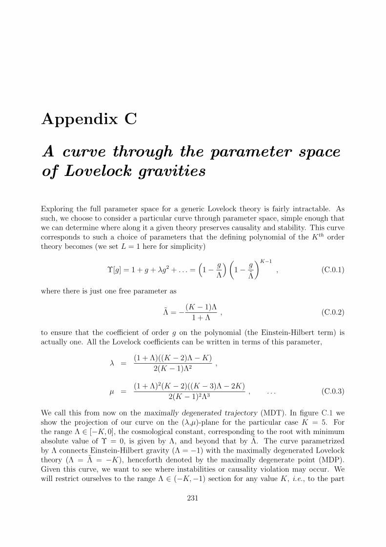
Appendix C
A curve through the parameter spaceof Lovelock gravities
Exploring the full parameter space for a generic Lovelock theory is fairly intractable. Assuch, we choose to consider a particular curve through parameter space, simple enough thatwe can determine where along it a given theory preserves causality and stability. This curvecorresponds to such a choice of parameters that the defining polynomial of the Kth ordertheory becomes (we set L = 1 here for simplicity)
Υ[g] = 1 + g + λg2 + . . . =(
1− g
Λ
)(1− g
Λ
)K−1
, (C.0.1)
where there is just one free parameter as
Λ = −(K − 1)Λ
1 + Λ, (C.0.2)
to ensure that the coefficient of order g on the polynomial (the Einstein-Hilbert term) isactually one. All the Lovelock coefficients can be written in terms of this parameter,
λ =(1 + Λ)((K − 2)Λ−K)
2(K − 1)Λ2,
µ =(1 + Λ)2(K − 2)((K − 3)Λ− 2K)
2(K − 1)2Λ3, . . . (C.0.3)
We call this from now on the maximally degenerated trajectory (MDT). In figure C.1 weshow the projection of our curve on the (λ,µ)-plane for the particular case K = 5. Forthe range Λ ∈ [−K, 0], the cosmological constant, corresponding to the root with minimumabsolute value of Υ = 0, is given by Λ, and beyond that by Λ. The curve parametrizedby Λ connects Einstein-Hilbert gravity (Λ = −1) with the maximally degenerated Lovelocktheory (Λ = Λ = −K), henceforth denoted by the maximally degenerate point (MDP).Given this curve, we want to see where instabilities or causality violation may occur. Wewill restrict ourselves to the range Λ ∈ (−K,−1) section for any value K, i.e., to the part
231
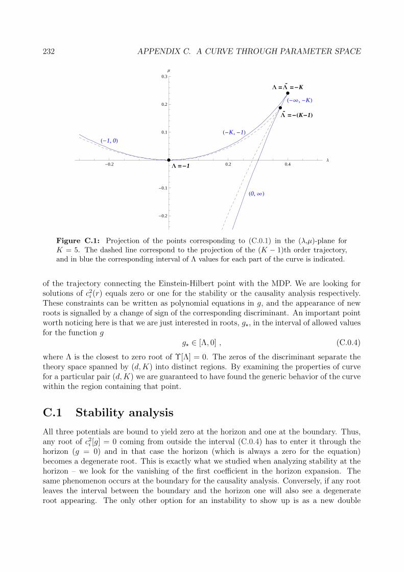
232 APPENDIX C. A CURVE THROUGH PARAMETER SPACE
-0.2 0.2 0.4Λ
-0.2
-0.1
0.1
0.2
0.3
Μ
H-1, 0LH-K, -1L
H-¥, -KL
H0, ¥L
L =-1
L =L
=-K
L
=-HK-1L
Figure C.1: Projection of the points corresponding to (C.0.1) in the (λ,µ)-plane forK = 5. The dashed line correspond to the projection of the (K − 1)th order trajectory,and in blue the corresponding interval of Λ values for each part of the curve is indicated.
of the trajectory connecting the Einstein-Hilbert point with the MDP. We are looking forsolutions of c2
i (r) equals zero or one for the stability or the causality analysis respectively.These constraints can be written as polynomial equations in g, and the appearance of newroots is signalled by a change of sign of the corresponding discriminant. An important pointworth noticing here is that we are just interested in roots, g?, in the interval of allowed valuesfor the function g
g? ∈ [Λ, 0] , (C.0.4)
where Λ is the closest to zero root of Υ[Λ] = 0. The zeros of the discriminant separate thetheory space spanned by (d,K) into distinct regions. By examining the properties of curvefor a particular pair (d,K) we are guaranteed to have found the generic behavior of the curvewithin the region containing that point.
C.1 Stability analysis
All three potentials are bound to yield zero at the horizon and one at the boundary. Thus,any root of c2
i [g] = 0 coming from outside the interval (C.0.4) has to enter it through thehorizon (g = 0) and in that case the horizon (which is always a zero for the equation)becomes a degenerate root. This is exactly what we studied when analyzing stability at thehorizon – we look for the vanishing of the first coefficient in the horizon expansion. Thesame phenomenon occurs at the boundary for the causality analysis. Conversely, if any rootleaves the interval between the boundary and the horizon one will also see a degenerateroot appearing. The only other option for an instability to show up is as a new double
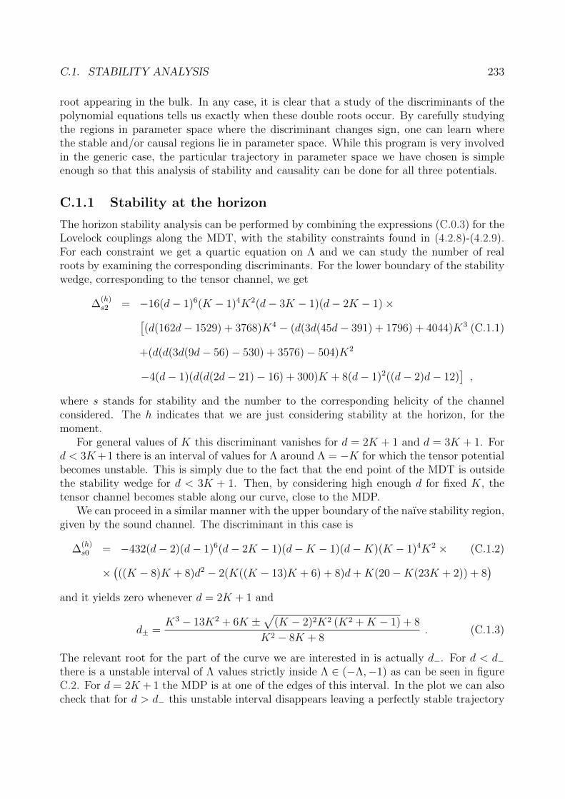
C.1. STABILITY ANALYSIS 233
root appearing in the bulk. In any case, it is clear that a study of the discriminants of thepolynomial equations tells us exactly when these double roots occur. By carefully studyingthe regions in parameter space where the discriminant changes sign, one can learn wherethe stable and/or causal regions lie in parameter space. While this program is very involvedin the generic case, the particular trajectory in parameter space we have chosen is simpleenough so that this analysis of stability and causality can be done for all three potentials.
C.1.1 Stability at the horizon
The horizon stability analysis can be performed by combining the expressions (C.0.3) for theLovelock couplings along the MDT, with the stability constraints found in (4.2.8)-(4.2.9).For each constraint we get a quartic equation on Λ and we can study the number of realroots by examining the corresponding discriminants. For the lower boundary of the stabilitywedge, corresponding to the tensor channel, we get
∆(h)s2 = −16(d− 1)6(K − 1)4K2(d− 3K − 1)(d− 2K − 1)×[
(d(162d− 1529) + 3768)K4 − (d(3d(45d− 391) + 1796) + 4044)K3 (C.1.1)
+(d(d(3d(9d− 56)− 530) + 3576)− 504)K2
−4(d− 1)(d(d(2d− 21)− 16) + 300)K + 8(d− 1)2((d− 2)d− 12)],
where s stands for stability and the number to the corresponding helicity of the channelconsidered. The h indicates that we are just considering stability at the horizon, for themoment.
For general values of K this discriminant vanishes for d = 2K + 1 and d = 3K + 1. Ford < 3K+1 there is an interval of values for Λ around Λ = −K for which the tensor potentialbecomes unstable. This is simply due to the fact that the end point of the MDT is outsidethe stability wedge for d < 3K + 1. Then, by considering high enough d for fixed K, thetensor channel becomes stable along our curve, close to the MDP.
We can proceed in a similar manner with the upper boundary of the naıve stability region,given by the sound channel. The discriminant in this case is
∆(h)s0 = −432(d− 2)(d− 1)6(d− 2K − 1)(d−K − 1)(d−K)(K − 1)4K2 × (C.1.2)
×(((K − 8)K + 8)d2 − 2(K((K − 13)K + 6) + 8)d+K(20−K(23K + 2)) + 8
)and it yields zero whenever d = 2K + 1 and
d± =K3 − 13K2 + 6K ±
√(K − 2)2K2 (K2 +K − 1) + 8
K2 − 8K + 8. (C.1.3)
The relevant root for the part of the curve we are interested in is actually d−. For d < d−there is a unstable interval of Λ values strictly inside Λ ∈ (−Λ,−1) as can be seen in figureC.2. For d = 2K + 1 the MDP is at one of the edges of this interval. In the plot we can alsocheck that for d > d− this unstable interval disappears leaving a perfectly stable trajectory
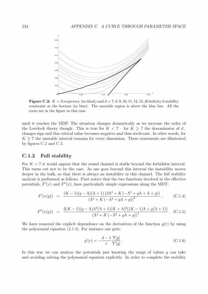
234 APPENDIX C. A CURVE THROUGH PARAMETER SPACE
0.20 0.25 0.30 0.35Λ
0.04
0.06
0.08
0.10
0.12
0.14
0.16
Μ
Figure C.2: K = 3 trajectory (in black) and d = 7, 8, 9, 10, 11, 12, 15, 20 helicity 0 stabilityconstraint at the horizon (in blue). The unstable region is above the blue line. All theroots are in the figure in this case.
until it reaches the MDP. The situation changes dramatically as we increase the order ofthe Lovelock theory though. This is true for K < 7 – for K ≥ 7 the denominator of d−changes sign and this critical value becomes negative and thus irrelevant. In other words, forK ≥ 7 the unstable interval remains for every dimension. These statements are illustratedby figures C.2 and C.3.
C.1.2 Full stability
For K > 7 it would appear that the sound channel is stable beyond the forbidden interval.This turns out not to be the case. As one goes beyond this interval the instability movesdeeper in the bulk, so that there is always an instability in this channel. The full stabilityanalysis is performed as follows. First notice that the two functions involved in the effectivepotentials, F ′(x) and F ′′(x), have particularly simple expressions along the MDT:
F ′(x(g)) =(K − 1)(g − Λ)(Λ + 1) (2Λ2 +K (−Λ2 + gΛ + Λ + g))
(Λ2 +K (−Λ2 + gΛ + g))2 , (C.1.4)
F ′′(x(g)) =2(K − 1)(g − Λ)Λ2(Λ + 1)(K + Λ)2((K − 1)Λ + g(Λ + 1))
(Λ2 +K (−Λ2 + gΛ + g))4 . (C.1.5)
We have removed the explicit dependence on the derivatives of the function g(r) by usingthe polynomial equation (2.1.8). For instance one gets:
g′(r) = −d− 1
r
Υ[g]
Υ′[g]. (C.1.6)
In this way we can analyze the potentials just knowing the range of values g can takeand avoiding solving the polynomial equation explicitly. In order to complete the stability
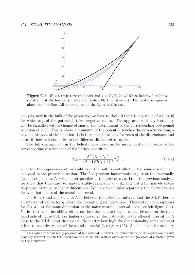
C.1. STABILITY ANALYSIS 235
0.30 0.35 0.40 0.45Λ
0.15
0.20
0.25
0.30
0.35
Μ
Figure C.3: K = 8 trajectory (in black) and d = 17, 20, 25, 30, 50,∞ helicity 0 stabilityconstraint at the horizon (in blue and dashed black for d → ∞). The unstable region isabove the blue line. All the roots are in the figure in this case.
analysis, now in the bulk of the geometry, we have to check if there is any value of g ∈ [Λ, 0]for which any of the potentials takes negative values. The appearance of any instabilitywill be signalled with a change of sign of the discriminant of the corresponding polynomialequation c2
i = 01. This is where a minimum of the potential touches the zero axis yielding anew double root of the equation. It is then enough to look for zeros of the discriminant andcheck if there is instabilities in the different disconnected regions.
The full discriminant in the helicity zero case can be nicely written in terms of thecorresponding discriminant of the horizon condition,
∆s0 =Λ12(K + Λ)12
(d− 1)12(Λ + 1)12∆
(h)s0 , (C.1.7)
and then the appearance of instabilities in the bulk is controlled by the same discriminantanalyzed in the precedent section. The Λ dependent factor vanishes just at the maximallysymmetric point as Λ = 0 is never possible in the present case. From the previous analysiswe know that there are two naively stable regions for d < d− and just a full naively stabletrajectory as we go to higher dimensions. We have to consider separately the allowed valuesfor Λ on both sides of the unstable interval.
For K < 7 and any value of Λ in between the forbidden interval and the MDP there isan interval of values for g where the potential goes below zero. This instability disappearsfor d > d−, at the same dimension as the naıve unstable interval does (see left figure C.4).Notice there’s no instability either on the other allowed region as can be seen on the righthand side of figure C.4. For higher values of K the instability in the allowed interval for Λclose to the MDP never disappears. No matter how high the dimensionality some values ofg lead to negative values of the sound potential (see figure C.5). As one enters the stability
1This equation is not really polynomial but rational. However the denominator of the expression doesn’tplay any relevant role in this discussion and so we will restrict ourselves to the polynomial equation givenby the numerator
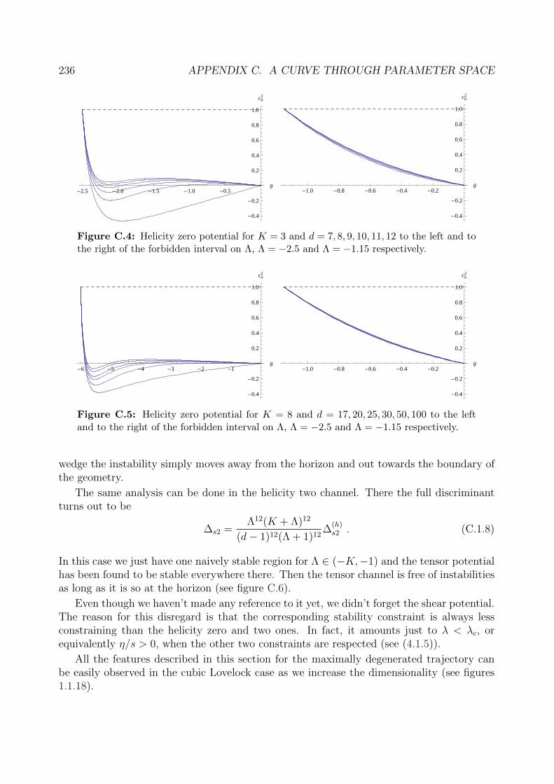
236 APPENDIX C. A CURVE THROUGH PARAMETER SPACE
-2.5 -2.0 -1.5 -1.0 -0.5g
-0.4
-0.2
0.2
0.4
0.6
0.8
1.0
c02
-1.0 -0.8 -0.6 -0.4 -0.2g
-0.4
-0.2
0.2
0.4
0.6
0.8
1.0
c02
Figure C.4: Helicity zero potential for K = 3 and d = 7, 8, 9, 10, 11, 12 to the left and tothe right of the forbidden interval on Λ, Λ = −2.5 and Λ = −1.15 respectively.
-6 -5 -4 -3 -2 -1g
-0.4
-0.2
0.2
0.4
0.6
0.8
1.0
c02
-1.0 -0.8 -0.6 -0.4 -0.2g
-0.4
-0.2
0.2
0.4
0.6
0.8
1.0
c02
Figure C.5: Helicity zero potential for K = 8 and d = 17, 20, 25, 30, 50, 100 to the leftand to the right of the forbidden interval on Λ, Λ = −2.5 and Λ = −1.15 respectively.
wedge the instability simply moves away from the horizon and out towards the boundary ofthe geometry.
The same analysis can be done in the helicity two channel. There the full discriminantturns out to be
∆s2 =Λ12(K + Λ)12
(d− 1)12(Λ + 1)12∆
(h)s2 . (C.1.8)
In this case we just have one naively stable region for Λ ∈ (−K,−1) and the tensor potentialhas been found to be stable everywhere there. Then the tensor channel is free of instabilitiesas long as it is so at the horizon (see figure C.6).
Even though we haven’t made any reference to it yet, we didn’t forget the shear potential.The reason for this disregard is that the corresponding stability constraint is always lessconstraining than the helicity zero and two ones. In fact, it amounts just to λ < λc, orequivalently η/s > 0, when the other two constraints are respected (see (4.1.5)).
All the features described in this section for the maximally degenerated trajectory canbe easily observed in the cubic Lovelock case as we increase the dimensionality (see figures1.1.18).
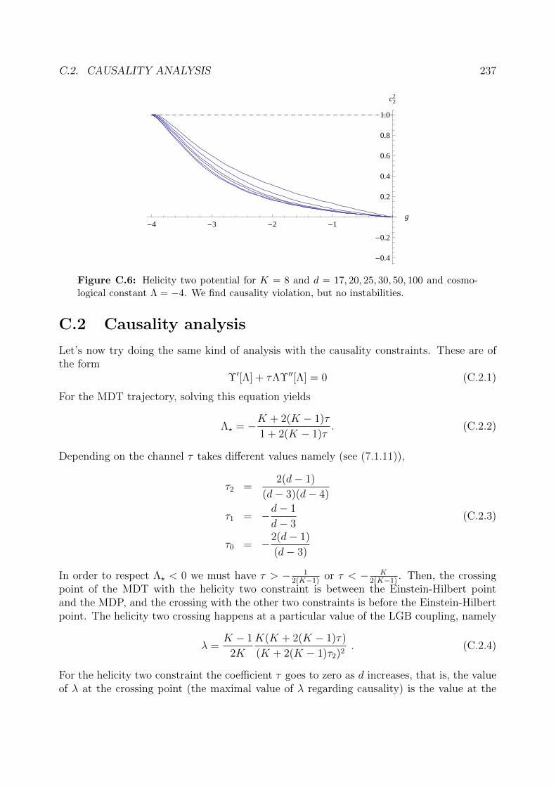
C.2. CAUSALITY ANALYSIS 237
-4 -3 -2 -1g
-0.4
-0.2
0.2
0.4
0.6
0.8
1.0
c22
Figure C.6: Helicity two potential for K = 8 and d = 17, 20, 25, 30, 50, 100 and cosmo-logical constant Λ = −4. We find causality violation, but no instabilities.
C.2 Causality analysis
Let’s now try doing the same kind of analysis with the causality constraints. These are ofthe form
Υ′[Λ] + τΛΥ′′[Λ] = 0 (C.2.1)
For the MDT trajectory, solving this equation yields
Λ? = −K + 2(K − 1)τ
1 + 2(K − 1)τ. (C.2.2)
Depending on the channel τ takes different values namely (see (7.1.11)),
τ2 =2(d− 1)
(d− 3)(d− 4)
τ1 = −d− 1
d− 3(C.2.3)
τ0 = −2(d− 1)
(d− 3)
In order to respect Λ? < 0 we must have τ > − 12(K−1)
or τ < − K2(K−1)
. Then, the crossingpoint of the MDT with the helicity two constraint is between the Einstein-Hilbert pointand the MDP, and the crossing with the other two constraints is before the Einstein-Hilbertpoint. The helicity two crossing happens at a particular value of the LGB coupling, namely
λ =K − 1
2K
K(K + 2(K − 1)τ)
(K + 2(K − 1)τ2)2. (C.2.4)
For the helicity two constraint the coefficient τ goes to zero as d increases, that is, the valueof λ at the crossing point (the maximal value of λ regarding causality) is the value at the
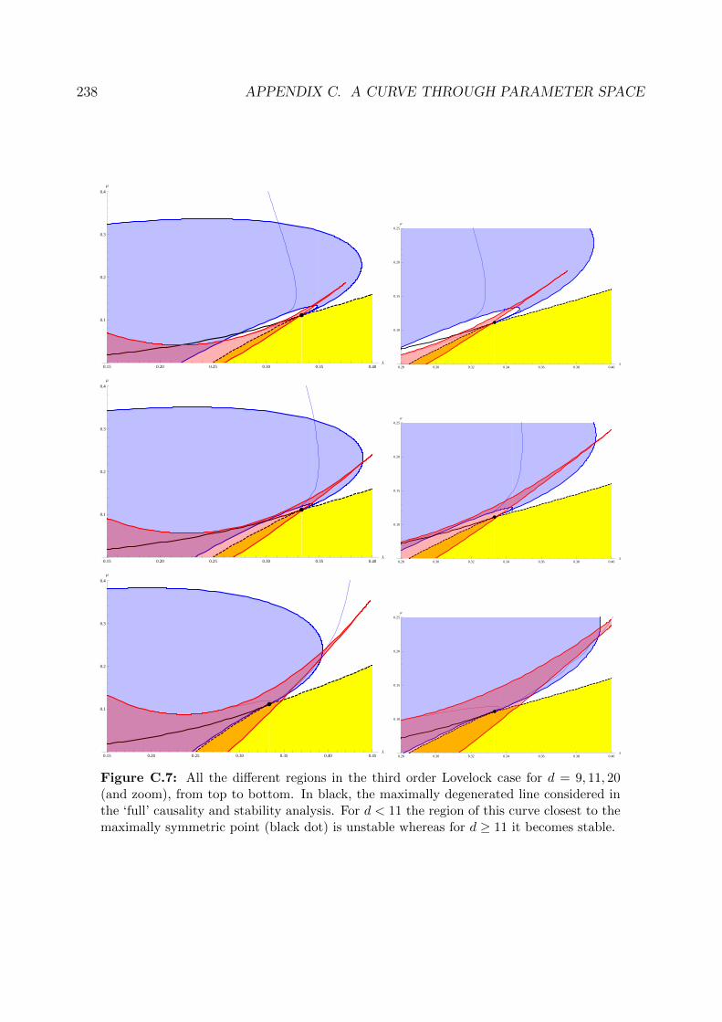
238 APPENDIX C. A CURVE THROUGH PARAMETER SPACE
0.15 0.20 0.25 0.30 0.35 0.40Λ
0.1
0.2
0.3
0.4
Μ
0.28 0.30 0.32 0.34 0.36 0.38 0.40Λ
0.10
0.15
0.20
0.25
Μ
0.15 0.20 0.25 0.30 0.35 0.40Λ
0.1
0.2
0.3
0.4
Μ
0.28 0.30 0.32 0.34 0.36 0.38 0.40Λ
0.10
0.15
0.20
0.25
Μ
0.15 0.20 0.25 0.30 0.35 0.40 0.45Λ
0.1
0.2
0.3
0.4
Μ
0.28 0.30 0.32 0.34 0.36 0.38 0.40Λ
0.10
0.15
0.20
0.25
Μ
Figure C.7: All the different regions in the third order Lovelock case for d = 9, 11, 20(and zoom), from top to bottom. In black, the maximally degenerated line considered inthe ‘full’ causality and stability analysis. For d < 11 the region of this curve closest to themaximally symmetric point (black dot) is unstable whereas for d ≥ 11 it becomes stable.
C.2. CAUSALITY ANALYSIS 239
maximally symmetric point with an increasing extra factor that goes to one as d → ∞.Then the crossing point approaches the MDP as d increases. This is explained by the factthat the helicity two causality reduces to CT ≥ 0 for d → ∞, and hence our trajectory canonly cross it at the MDP itself.
The full causality analysis is quite more complicated that the stability one and not veryenlightening. Here we will simply cite some partial results in the most relevant case, thehelicity two one. In that case the equation c2
2(r) = 1 can be reduced to a polynomial equationon g with discriminant
∆c2 = Λ20(1 + Λ)12(K + Λ)12 (Λ− Λ?) ∆c2. (C.2.5)
The factor ∆c2 is a complicated expression which has zeroes at points irrelevant for ouranalysis. In particular, when restricted to the part of the curve connecting the Einstein-Hilbert point with the maximally symmetric point (Λ ∈ (−K,−1)) the discriminant hasjust one relevant root at Λ = Λ?, exactly the point determined by demanding causality atthe boundary. The situation is analogous for the other two helicities. Then, causality inthe MDT reduces to causality at the boundary. In particular, close to the MDP the onlyconstraint comes from the helicity two channel, as has been discussed.
In the same way as for the stability analysis, all the previously referred features can beseen in the third order case (see figures 1.1.18).
240 APPENDIX C. A CURVE THROUGH PARAMETER SPACE
Appendix D
Cavitation effects on theconfinement/deconfinementtransition
Hydrodynamics is a universal framework to describe strongly coupled systems at energyscales much lower than their characteristic microscopic scales (masses, temperature, etc).The basic hydrodynamic equation is that of the conservation of the stress-energy tensor
∇µTµν = 0 . (D.0.1)
For an ideal relativistic fluid the stress-energy tensor takes the form
T µνideal = E uµuν + P ∆µν , (D.0.2)
where E and P are the energy density and pressure,
∆µν = gµν + uµuν ,
and uµ is the fluid four-velocity, normalized so that uµuµ = −1. The leading viscous correc-
tions are parametrized by the fluid shear η and bulk ζ transport coefficients in the viscoustensor Πµν :
T µν = T µνideal + Πµν , (D.0.3)
Πµν = −η σµν − ζ ∇u ∆µν , (D.0.4)
where ∇u ≡ ∇αuα, and we have adopted
σµν =(∆µλ∇λu
ν + ∆νλ∇λuµ)− 2
3∇u ∆µν . (D.0.5)
Assuming that the relevant microscopic scale is the temperature, leading hydrodynamicapproximation is valid provided
|∇µuν |
T 1 , (D.0.6)
241
242 APPENDIX D. CAVITATION EFFECTS
otherwise, higher-order gradients (typically infinitely many of them) must be included [273–275].
It is easy to see that viscous terms tend to reduce the pressure [276]. For example, forfluids comoving in an expanding background such as an FRW metric,
ds24 = −dt2 + a(t)2(d~x)2 , (D.0.7)
we find
σµν∣∣FRW
= 0 , ∇u∣∣FRW
= 3a
a, (D.0.8)
resulting in an isotropic effective pressure
Peff = P − ζ ∇u . (D.0.9)
In the case of a boost invariant fluid expansion, the pressure is no longer isotropic [274]:
Peff⊥ = P +
2η − 3ζ
3τ, Peff
ξ = P − 4η + 3ζ
3τ, (D.0.10)
where ⊥ and ξ are the transverse and longitudinal directions of the boost invariant expansion1,and τ is the proper time. Notice that in this case the spatially averaged pressure,
(23P⊥ + 1
3Pξ)
still takes the form (D.0.9). In what follows, we take the trace-averaged form (D.0.9) as ageneric expression for the effective pressure.
Consider now a system which, in thermal equilibrium, can exist in one of the two phasesA or B. A first-order phase transition between these phases implies the existence of a criticaltemperature Tc, such that PA > PB for T > Tc, and PA < PB otherwise. The phase withthe higher pressure is thermodynamically favoured, and the transition at T = Tc proceedsthrough nucleation of bubbles of a stable phase. If the system flows, the relevant pressuredetermining the stability of a phase is the effective one:
PeffA/B = PA/B − ζA/B ∇u . (D.0.11)
Close2 to Tc,PA/B = Pc + SA/B (T − Tc) +O
((T − Tc)2
), (D.0.12)
where SA/B are the entropy densities of the corresponding phases. Thus, viscous hydrody-namics effects would shift the transition temperature according to
|δTc|Tc
∼ |ζA − ζB||SA − SB|
|∇u|Tc
.|ζA − ζB||SA − SB|
, (D.0.13)
where the upper bound is enforced from the consistency of truncating hydrodynamics at thefirst order in the velocity gradients, see (D.0.6). Notice that cavitation affects the transitiontemperature the more weakly the first-order transition is (the smaller the difference betweenSA/B is), and the larger the bulk viscosity difference of the two phases at Tc is.
1Such expansion is conveniently described changing variables from (t, z) to (τ, ξ): τ =√t2 − z2, ξ =
arctanh zt .2We use the first law of thermodynamics dF = −dP = −S dT .
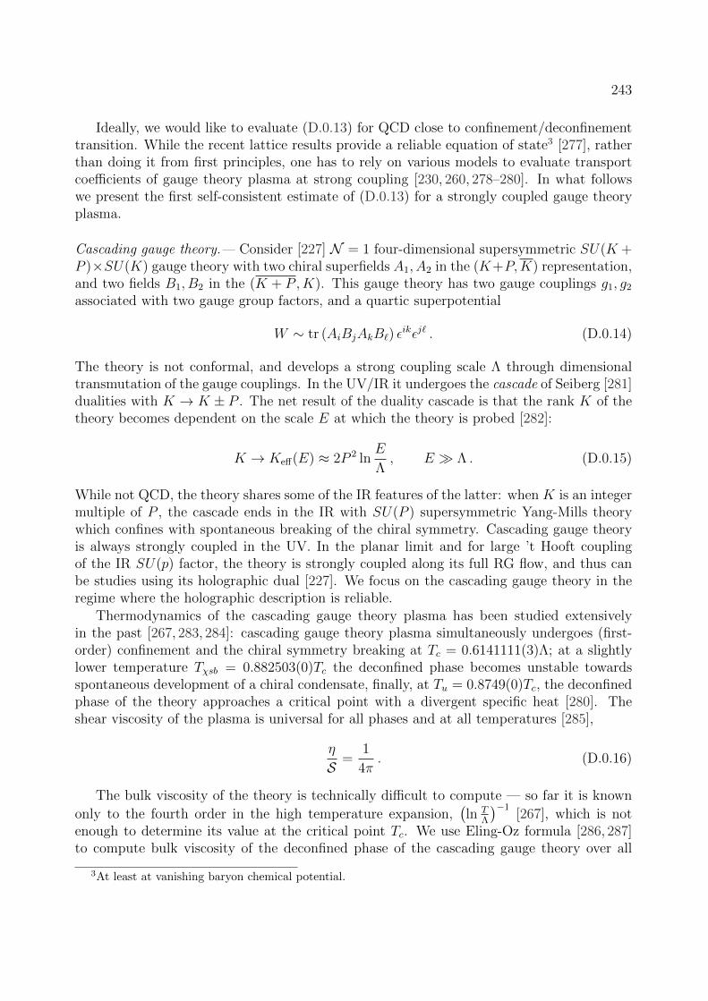
243
Ideally, we would like to evaluate (D.0.13) for QCD close to confinement/deconfinementtransition. While the recent lattice results provide a reliable equation of state3 [277], ratherthan doing it from first principles, one has to rely on various models to evaluate transportcoefficients of gauge theory plasma at strong coupling [230, 260, 278–280]. In what followswe present the first self-consistent estimate of (D.0.13) for a strongly coupled gauge theoryplasma.
Cascading gauge theory.— Consider [227] N = 1 four-dimensional supersymmetric SU(K +P )×SU(K) gauge theory with two chiral superfields A1, A2 in the (K+P,K) representation,and two fields B1, B2 in the (K + P ,K). This gauge theory has two gauge couplings g1, g2
associated with two gauge group factors, and a quartic superpotential
W ∼ tr (AiBjAkB`) εikεj` . (D.0.14)
The theory is not conformal, and develops a strong coupling scale Λ through dimensionaltransmutation of the gauge couplings. In the UV/IR it undergoes the cascade of Seiberg [281]dualities with K → K ± P . The net result of the duality cascade is that the rank K of thetheory becomes dependent on the scale E at which the theory is probed [282]:
K → Keff(E) ≈ 2P 2 lnE
Λ, E Λ . (D.0.15)
While not QCD, the theory shares some of the IR features of the latter: when K is an integermultiple of P , the cascade ends in the IR with SU(P ) supersymmetric Yang-Mills theorywhich confines with spontaneous breaking of the chiral symmetry. Cascading gauge theoryis always strongly coupled in the UV. In the planar limit and for large ’t Hooft couplingof the IR SU(p) factor, the theory is strongly coupled along its full RG flow, and thus canbe studies using its holographic dual [227]. We focus on the cascading gauge theory in theregime where the holographic description is reliable.
Thermodynamics of the cascading gauge theory plasma has been studied extensivelyin the past [267, 283, 284]: cascading gauge theory plasma simultaneously undergoes (first-order) confinement and the chiral symmetry breaking at Tc = 0.6141111(3)Λ; at a slightlylower temperature Tχsb = 0.882503(0)Tc the deconfined phase becomes unstable towardsspontaneous development of a chiral condensate, finally, at Tu = 0.8749(0)Tc, the deconfinedphase of the theory approaches a critical point with a divergent specific heat [280]. Theshear viscosity of the plasma is universal for all phases and at all temperatures [285],
η
S=
1
4π. (D.0.16)
The bulk viscosity of the theory is technically difficult to compute — so far it is known
only to the fourth order in the high temperature expansion,(ln T
Λ
)−1[267], which is not
enough to determine its value at the critical point Tc. We use Eling-Oz formula [286, 287]to compute bulk viscosity of the deconfined phase of the cascading gauge theory over all
3At least at vanishing baryon chemical potential.
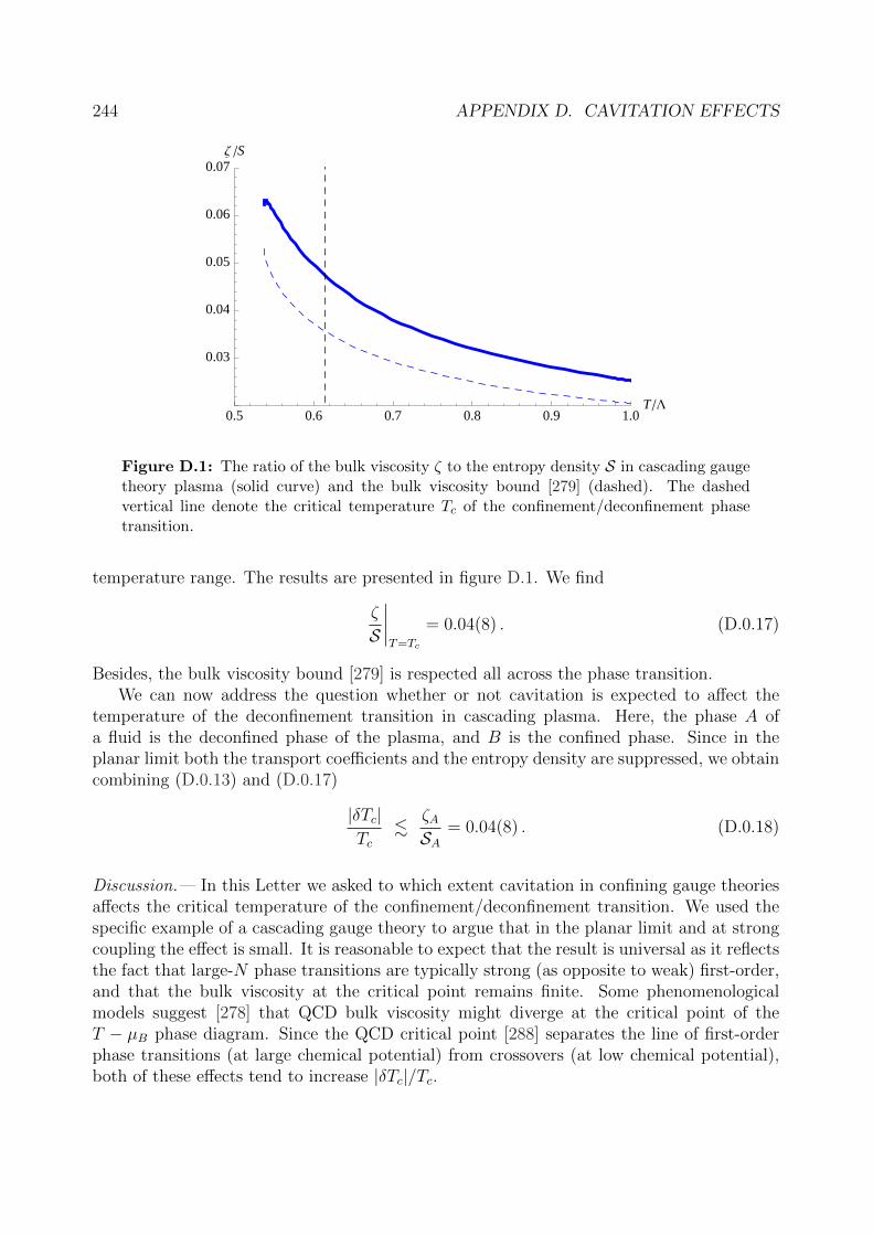
244 APPENDIX D. CAVITATION EFFECTS
0.5 0.6 0.7 0.8 0.9 1.0TL
0.03
0.04
0.05
0.06
0.07Ζ S
Figure D.1: The ratio of the bulk viscosity ζ to the entropy density S in cascading gaugetheory plasma (solid curve) and the bulk viscosity bound [279] (dashed). The dashedvertical line denote the critical temperature Tc of the confinement/deconfinement phasetransition.
temperature range. The results are presented in figure D.1. We find
ζ
S
∣∣∣∣T=Tc
= 0.04(8) . (D.0.17)
Besides, the bulk viscosity bound [279] is respected all across the phase transition.We can now address the question whether or not cavitation is expected to affect the
temperature of the deconfinement transition in cascading plasma. Here, the phase A ofa fluid is the deconfined phase of the plasma, and B is the confined phase. Since in theplanar limit both the transport coefficients and the entropy density are suppressed, we obtaincombining (D.0.13) and (D.0.17)
|δTc|Tc
.ζASA
= 0.04(8) . (D.0.18)
Discussion.— In this Letter we asked to which extent cavitation in confining gauge theoriesaffects the critical temperature of the confinement/deconfinement transition. We used thespecific example of a cascading gauge theory to argue that in the planar limit and at strongcoupling the effect is small. It is reasonable to expect that the result is universal as it reflectsthe fact that large-N phase transitions are typically strong (as opposite to weak) first-order,and that the bulk viscosity at the critical point remains finite. Some phenomenologicalmodels suggest [278] that QCD bulk viscosity might diverge at the critical point of theT − µB phase diagram. Since the QCD critical point [288] separates the line of first-orderphase transitions (at large chemical potential) from crossovers (at low chemical potential),both of these effects tend to increase |δTc|/Tc.
Bibliography
[1] X. O. Camanho and J. D. Edelstein, “Causality constraints in AdS/CFT fromconformal collider physics and Gauss-Bonnet gravity,” JHEP 1004 (2010) 007,arXiv:0911.3160 [hep-th].
[2] X. O. Camanho and J. D. Edelstein, “Causality in AdS/CFT and Lovelock theory,”JHEP 1006 (2010) 099, arXiv:0912.1944 [hep-th].
[3] X. O. Camanho, J. D. Edelstein and M. F. Paulos, “Lovelock theories, holographyand the fate of the viscosity bound,” JHEP 1105 (2011) 127, arXiv:1010.1682[hep-th].
[4] X. O. Camanho and J. D. Edelstein, “A Lovelock black hole bestiary,” Class.Quantum Grav. 30 (2013) 035009, arXiv:1103.3669 [hep-th].
[5] X. O. Camanho, J. D. Edelstein, G. Giribet and A. Gomberoff, “New type of phasetransition in gravitational theories,” Phys. Rev. D86 (2012) 124048,arXiv:1204.6737 [hep-th].
[6] X. O. Camanho, “Phase transitions in general gravity theories,” Progress inMathematical Relativity, Gravitation and Cosmology, Springer Proc. Math. Stat. 60(2014) 167, arXiv:1303.6222 [gr-qc].
[7] A. Buchel, X. O. Camanho and J. D. Edelstein, “Cavitation effects on theconfinement/deconfinement transition,” Phys. Lett. B734 (2014) 131,arXiv:1303.6300 [hep-ph].
[8] X. O. Camanho and J. D. Edelstein, “Cosmic censorship in Lovelock theory,” JHEP1311 (2013) 151, arXiv:1308.0304 [hep-th].
[9] X. O. Camanho, J. D. Edelstein, G. Giribet and A. Gomberoff, “GeneralizedHawking-Page transitions in Lovelock gravity,” Phys. Rev. D90 (2014) 064028,arXiv:1311.6768 [hep-th].
[10] X. O. Camanho, J. D. Edelstein, J. Maldacena and A. Zhiboedov, ”Causalityconstraints on corrections to the graviton three-point coupling,” arXiv:1407.5597
[hep-th].
[11] T. Eguchi, P. B. Gilkey, and A. J. Hanson, “Gravitation, Gauge Theories andDifferential Geometry,” Phys.Rept. 66 (1980) 213.
245
246 BIBLIOGRAPHY
[12] S. Willison, “Intersecting hypersurfaces in AdS and Lovelock Gravity,” PhD Thesis(2005) 109, arXiv:0412273 [gr-qc].
[13] A. Einstein, “Die Grundlage der allgemeinen Relativitatstheorie [AdP 49, 769(1916)],” Ann. Phys. 14 (2005) 517–571.
[14] A. Einstein, “Zur Elektrodynamik bewegter Korper [AdP 17, 891 (1905)],” Ann.Phys. 14 (2005) 194–224.
[15] D. Lovelock, “The Einstein tensor and its generalizations,” J. Math. Phys. 12 (1971)498–501.
[16] A. Einstein, “Cosmological Considerations in the General Theory of Relativity,”Sitzungsber.Preuss.Akad.Wiss.Berlin (Math.Phys.) 1917 (1917) 142–152.
[17] H. Vermeil Nachr. Ges. Wiss. Gottingen (1917) 334.
[18] H. Weyl, Raum, Zeit, Materie:, 4th ed. Springer, Berlin, 1921.
[19] E. Cartan J. Math. Pures Appl. 1 (1922) 141.
[20] N. Deruelle and J. Madore, “On the quasi-linearity of the Einstein-Gauss-Bonnetgravity field equations,” arXiv:0305004 [gr-qc].
[21] C. Lanczos Z. Phys. 73 (1932) 147.
[22] C. Lanczos, “A Remarkable property of the Riemann-Christoffel tensor in fourdimensions,” Annals Math. 39 (1938) 842–850.
[23] A. Adams, N. Arkani-Hamed, S. Dubovsky, A. Nicolis, and R. Rattazzi, “Causality,analyticity and an IR obstruction to UV completion,” JHEP 10 (2006) 014–014.arXiv:0602178 [hep-th].
[24] T. Kaluza, “On the Problem of Unity in Physics,”Sitzungsber.Preuss.Akad.Wiss.Berlin (Math.Phys.) 1921 (1921) 966–972.
[25] O. Klein, “Quantentheorie und funfdimensionale Relativitatstheorie,” Zeitschrift furPhysik 37 (1926) 895–906.
[26] A. Eddington, The Mathematical Theory of Relativity, 2nd ed. Cambridge UniversityPress, England, 1924.
[27] D. G. Boulware, The Quantum Theory of Gravity. Hilger, London, 1984.
[28] N. Birrell and P. Davies, Quantum Fields in Curved Spacetimes. CambridgeUniversity Press, England, 1982.
[29] B. Zwiebach, “Curvature Squared Terms and String Theories,” Phys. Lett. B156(1985) 315.
BIBLIOGRAPHY 247
[30] J. M. Maldacena, “The large N limit of superconformal field theories andsupergravity,” Adv. Theor. Math. Phys. 2 (1998) 231–252, arXiv:9711200 [hep-th].
[31] I. R. Klebanov and E. Witten, “Superconformal field theory on threebranes at aCalabi-Yau singularity,” Nucl. Phys. B536 (1998) 199–218, arXiv:9807080[hep-th].
[32] A. M. Polyakov, “The wall of the cave,” Int. J. Mod. Phys. A14 (1999) 645–658,arXiv:9809057 [hep-th].
[33] A. Strominger, “Black hole entropy from near horizon microstates,” JHEP 9802(1998) 009, arXiv:9712251 [hep-th].
[34] J. D. Brown and M. Henneaux, “Central charges in the canonical realization ofasymptotic symmetries: an example from three-dimensional gravity,” Commun.Math. Phys. 104 (1986) 207–226.
[35] E. Witten, “Conformal Field Theory In Four And Six Dimensions,”arXiv:0712.0157 [math.RT].
[36] J. de Boer, M. Kulaxizi, and A. Parnachev, “AdS7/CFT6, Gauss-Bonnet Gravity,and Viscosity Bound,” JHEP 03 (2010) 087, arXiv:0910.5347 [hep-th].
[37] A. Buchel, J. Escobedo, R. C. Myers, M. F. Paulos, A. Sinha, and M. Smolkin,“Holographic GB gravity in arbitrary dimensions,” JHEP 03 (2010) 111,arXiv:0911.4257 [hep-th].
[38] J. de Boer, M. Kulaxizi, and A. Parnachev, “Holographic Lovelock gravities andblack holes,” JHEP 06 (2010) 008, arXiv:0912.1877 [hep-th].
[39] M. Kulaxizi and A. Parnachev, “Energy Flux Positivity and Unitarity in ConformalField Theories,” Phys. Rev. Lett. 106 (2011) 011601, arXiv:1007.0553 [hep-th].
[40] M. F. Paulos, “Holographic phase space: c-functions and black holes asrenormalization group flows,” JHEP 05 (2011) 043, arXiv:1101.5993 [hep-th].
[41] B. Zumino, “Gravity Theories in More Than Four-Dimensions,” Phys. Rept. 137(1986) 109.
[42] A. H. Chamseddine, “Topological gauge theory of gravity in five-dimensions and allodd dimensions,” Phys. Lett. B233 (1989) 291.
[43] J. Zanelli, “Lecture notes on Chern-Simons (super-)gravities,” arXiv:0502193
[hep-th].
[44] D. G. Boulware and S. Deser, “String Generated Gravity Models,” Phys. Rev. Lett.55 (1985) 2656.
[45] C. Charmousis and A. Padilla, “The Instability of Vacua in Gauss-Bonnet Gravity,”JHEP 12 (2008) 038, arXiv:0807.2864 [hep-th].
248 BIBLIOGRAPHY
[46] J. W. York, “Role of Conformal Three-Geometry in the Dynamics of Gravitation,”Phys. Rev. Lett. 28 (1972) 1082–1085.
[47] G. W. Gibbons and S. W. Hawking, “Action Integrals and Partition Functions inQuantum Gravity,” Phys. Rev. D15 (1977) 2752–2756.
[48] R. Myers, “Higher-derivative gravity, surface terms, and string theory,” Phys. Rev.D36 (1987) 392–396.
[49] W. Israel, “Singular hypersurfaces and thin shells in general relativity,” Il NuovoCimento B Series 10 48 (1967) 463–463.
[50] G. Hayward and J. Louko, “Variational principles for nonsmooth metrics,” Phys.Rev. D42 (1990) 4032–4041.
[51] E. Gravanis and S. Willison, “Israel conditions for the Gauss-Bonnet theory and theFriedmann equation on the brane universe,” Phys. Lett. B562 (2003) 118–126,arXiv:0209076 [hep-th].
[52] K.-i. Maeda and T. Torii, “Covariant gravitational equations on a brane world with aGauss-Bonnet term,” Phys. Rev. D69 (2004) 024002, arXiv:0309152 [hep-th].
[53] E. Gravanis and S. Willison, “Intersecting hyper-surfaces in dimensionally continuedtopological density gravitation,” J. Math. Phys. 45 (2004) 4223-4238,arXiv:0306220 [hep-th].
[54] S. Davis, “Generalized Israel junction conditions for a Gauss-Bonnet brane world,”Phys. Rev. D67 (2003) 024030, arXiv:0208205 [hep-th].
[55] E. Gravanis and S. Willison, ““Mass without mass” from thin shells in Gauss-Bonnetgravity,” Phys. Rev. D75 (2007) 13, arXiv:0701152 [gr-qc].
[56] C. Garraffo, G. Giribet, E. Gravanis, and S. Willison, “Gravitational solitons and C0
vacuum metrics in five-dimensional Lovelock gravity,” J. Math. Phys. 49 (2008)042502, arXiv:0711.2992 [gr-qc].
[57] C. Teitelboim and J. Zanelli, “Dimensionally continued topological gravitation theoryin Hamiltonian form,” Class. Quantum Grav. 4 (1987) L125–L129.
[58] M. Banados, C. Teitelboim, and J. Zanelli, “Black hole entropy and the dimensionalcontinuation of the Gauss-Bonnet theorem,” Phys. Rev. Lett. 72 (1994) 957–960,arXiv:9309026 [gr-qc].
[59] O. Miskovic and R. Olea, “Counterterms in Dimensionally Continued AdS Gravity,”JHEP (2007) 26, arXiv:0706.4460 [hep-th].
[60] K. Schwarzschild, “On the gravitational field of a mass point according to Einstein’stheory,” Sitzungsber.Preuss.Akad.Wiss.Berlin (Math.Phys.) 1916 (1916) 189–196.
BIBLIOGRAPHY 249
[61] S. Chandrasekhar, “The maximum mass of ideal white dwarfs,” Astrophys.J. 74(1931) 81–82.
[62] J. R. Oppenheimer and G. M. Volkoff, “On Massive Neutron Cores,” Phys. Rev. 55(1939) 374–381.
[63] R. Penrose, “Gravitational Collapse and Space-Time Singularities,” Phys. Rev. Lett.14 (1965) 57–59.
[64] S. Hawking, “Occurrence of Singularities in Open Universes,” Phys. Rev. Lett. 15(1965) 689–690.
[65] J. Michell, “On the Means of Discovering the Distance, Magnitude, etc. of the FixedStars, in Consequence of the Diminution of the Velocity of Their Light, in Case Sucha Diminution Should be Found to Take Place in any of Them, and Such Other DataShould be Procured from Observations, as Would be Farther Necessary for ThatPurpose. By the Rev. John Michell, B. D. F. R. S. In a Letter to Henry Cavendish,Esq. F. R. S. and A. S.,” Philosophical Transactions of the Royal Society of London74 (1784) pp. 35–57. http://www.jstor.org/stable/106576.
[66] R. Penrose, “Gravitational collapse: The role of general relativity,” Riv. Nuovo Cim.1 (1969) 252 [Gen. Rel. Grav. 34 (2002) 1141].
[67] J. Oliva and S. Ray, “A new cubic theory of gravity in five dimensions: Black hole,Birkhoff’s theorem and C-function,” Class. Quantum Grav. 27 (2010) 225002,arXiv:1003.4773 [gr-qc].
[68] J. Oliva and S. Ray, “A Classification of Six Derivative Lagrangians of Gravity andStatic Spherically Symmetric Solutions,” Phys. Rev. D82 (2010) 124030,arXiv:1004.0737 [gr-qc].
[69] R. C. Myers and B. Robinson, “Black holes in quasi-topological gravity,” JHEP 08(2010) 067, arXiv:1003.5357 [gr-qc].
[70] J. Oliva and S. Ray, “Birkhoff’s theorem in higher derivative theories of gravity,”Class. Quantum Grav. 28 (2011) 175007, arXiv:1104.1205 [gr-qc].
[71] R. C. Myers, M. F. Paulos, and A. Sinha, “Holographic studies of quasi-topologicalgravity,” JHEP 08 (2010) 035, arXiv:1004.2055 [hep-th].
[72] R. Aros, R. Troncoso, and J. Zanelli, “Black holes with topologically nontrivial AdSasymptotics,” Phys.Rev. D 63 (2001) 084015, arXiv/0011097 [hep-th].
[73] J. A. Wolf, Spaces of constant curvature. AMS Chelsea Publishing ChelseaPublishing, Providence, Rhode Island, 6th ed., 2011.
[74] R. Zegers, “Birkhoff’s theorem in Lovelock gravity,” J. Math. Phys. 46 (2005)072502, arXiv:0505016 [gr-qc].
250 BIBLIOGRAPHY
[75] C. Charmousis and J.-F. Dufaux, “General Gauss-Bonnet brane cosmology,” Class.Quantum Grav. 19 (2002) 4671–4682, arXiv:0202107 [hep-th].
[76] R. Emparan, “AdS/CFT duals of topological black holes and the entropy ofzero-energy states,” JHEP 06 (1999) 036–036, arXiv:9906040 [hep-th].
[77] D. Kastor, S. Ray, and J. Traschen, “Smarr Formula and an Extended First Law forLovelock Gravity,” Class. Quantum Grav. 27 (2010) 235014, arxiv:1005.5053[hep-th].
[78] D. Kastor, S. Ray, and J. Traschen, “Mass and free energy of Lovelock black holes,”Class. Quantum Grav. 28 (2011) 195022, arXiv:1106.2764 [hep-th].
[79] J. T. Wheeler, “Symmetric Solutions to the Gauss-Bonnet Extended EinsteinEquations,” Nucl. Phys. B268 (1986) 737.
[80] J. T. Wheeler, “Symmetric solutions to the maximally Gauss-Bonnet extendedEinstein equations,” Nucl. Phys. B273 (1986) 732.
[81] R.-G. Cai and K.-S. Soh, “Topological black holes in the dimensionally continuedgravity,” Phys. Rev. D59 (1999) 044013, arXiv:9808067 [gr-qc].
[82] M. Marden, “Geometry of polynomials,” Mathematical Surveys and Monographs 3243. Providence, USA: Am. Math. Soc. (1949) 243 p.
[83] R. B. Mann, “Black holes of negative mass,” Class. Quantum Grav. 14 (1997)2927–2930, arXiv:9705007 [gr-qc].
[84] G. T. Horowitz and R. C. Myers, “The AdS/CFT Correspondence and a NewPositive Energy Conjecture for General Relativity,” Phys. Rev. D59 (1998) 026005,arXiv:9808079 [hep-th].
[85] R. W. D. Nickalls, “A new approach to solving the cubic: Cardan’s solutionrevealed,” Math. Gazette 77 (1993) 354–359.
[86] M. H. Dehghani and R. Pourhasan, “Thermodynamic instability of black holes ofthird order Lovelock gravity,” Phys. Rev. D79 (2009) 064015, arXiv:0903.4260[gr-qc].
[87] X.-H. Ge, S.-J. Sin, S.-F. Wu, and G.-H. Yang, “Shear viscosity and instability fromthird order Lovelock gravity,” Phys. Rev. D80 (2009) 104019, arXiv:0905.2675[hep-th].
[88] D. Wiltshire, “Spherically symmetric solutions of Einstein-Maxwell theory with aGauss-Bonnet term,” Phys. Lett. B169 (1986) 36–40.
[89] D. Wiltshire, “Black holes in string-generated gravity models,” Phys. Rev. B38(1988) 2445–2456.
BIBLIOGRAPHY 251
[90] J. E. Lidsey, S. Nojiri, and S. D. Odintsov, “Braneworld cosmology in (anti)-de SitterEinstein-Gauss-Bonnet-Maxwell gravity,” JHEP 06 (2002) 026–026, arXiv:0202198[hep-th].
[91] M. Cvetic, S. Nojiri, and S. Odintsov, “Black hole thermodynamics and negativeentropy in deSitter and anti-deSitter Einstein-Gauss-Bonnet gravity,” Nucl. Phys.B628 (2002) 295–330, arXiv:0112045 [hep-th].
[92] M. Aiello, R. Ferraro, and G. Giribet, “Exact solutions of Lovelock-Born-Infeld blackholes,” Phys. Rev. D70 (2004) 9, arXiv:0408078 [gr-qc].
[93] M. Banados, “Charged black holes in Gauss-Bonnet extended gravity,” Phys. Lett.B579 (2004) 13–24, arXiv:0310160 [hep-th].
[94] M. Aiello, R. Ferraro, and G. Giribet, “Hoffmann-Infeld black-hole solutions inLovelock gravity,” Class. Quantum Grav. 22 (2005) 2579–2588, arXiv:0502069[gr-qc].
[95] T. Torii and H. Maeda, “Spacetime structure of static solutions in Gauss-Bonnetgravity: Charged case,” Phys. Rev. D72 (2005) 064007, arXiv:0504141 [hep-th].
[96] H. Maeda, M. Hassaıne, and C. Martınez, “Lovelock black holes with a nonlinearMaxwell field,” Phys. Rev. D79 (2009) 044012, arXiv:0812.2038 [gr-qc].
[97] P. Li, R.-H. Yue, and D.-C. Zou, “Thermodynamics of Third OrderLovelock-Born-Infeld Black Holes,” Commun. Theor. Phys. 56 (2011) 845-850,arXiv:1110.0064 [gr-qc].
[98] N. Ohta and T. Torii, “Charged Black Holes in String Theory with Gauss-BonnetCorrection in Various Dimensions,” Phys. Rev. D86 (2012) 104016,arXiv:1208.6367 [hep-th].
[99] M. Dehghani, “Charged rotating black branes in anti-de Sitter Einstein-Gauss-Bonnetgravity,” Phys. Rev. D67 (2003) 064017, arXiv:0211191 [hep-th].
[100] M. Dehghani and M. Shamirzaie, “Thermodynamics of asymptotically flat chargedblack holes in third order Lovelock gravity,” Phys. Rev. D72 (2005) 124015.
[101] M. Dehghani and R. Mann, “Thermodynamics of rotating charged black branes inthird order lovelock gravity and the counterterm method,” Phys. Rev. D73 (2006)104003.
[102] M. Dehghani, N. Alinejadi, and S. Hendi, “Topological black holes inLovelock-Born-Infeld gravity,” Phys. Rev. D77 (2008) 104025, arXiv:0802.2637[hep-th].
[103] T. Takahashi, “Fatal Effects of Charges on Stability of Black Holes in LovelockTheory,” Prog. Theor. Phys. 125 (2011) 1289–1310, arXiv:1102.1785 [gr-qc].
252 BIBLIOGRAPHY
[104] T. Takahashi, “Instability of Charged Lovelock Black Holes: Vector Perturbationsand Scalar Perturbations,” arXiv:1209.2867 [gr-qc].
[105] W. G. Brenna and R. B. Mann, “Quasi-topological Reissner-Nordstrom Black Holes,”Phys. Rev. D86 (2012) 064035, arXiv:1206.4738 [hep-th].
[106] B. Wang, R.-K. Su, P. Yu, and E. Young, “Can a nonextremal Reissner-Nordstromblack hole become extremal by assimilating an infalling charged particle and shell?,”Phys. Rev. D57 (1998) 5284–5286.
[107] A. Anabalon, N. Deruelle, Y. Morisawa, J. Oliva, M. Sasaki, D. Tempo, andR. Troncoso, “Kerr-Schild ansatz in Einstein-Gauss-Bonnet gravity: an exact vacuumsolution in five dimensions,” Class. Quantum Grav. 26 (2009) 065002,arXiv:0812.3194 [hep-th].
[108] Y. Brihaye and E. Radu, “Five-dimensional rotating black holes inEinstein-Gauss-Bonnet theory,” Phys. Lett. B661 (2008) 167–174, arXiv:0801.1021[hep-th].
[109] H.-C. Kim and R.-G. Cai, “Slowly rotating charged Gauss-Bonnet black holes in AdSspaces,” Phys. Rev. D77 (2008) 024045, arXiv:0711.0885 [hep-th].
[110] V. Faraoni, “Cosmological apparent and trapping horizons,” Phys. Rev. D84 (2011)024003, arXiv:1106.4427 [gr-qc].
[111] H. Maeda, “Gauss-Bonnet braneworld redux: A novel scenario for the bouncinguniverse,” Phys. Rev. D85 (2012) 124012, arXiv:1112.5178 [hep-th].
[112] J. D. Bekenstein, “Black holes and entropy,” Phys. Rev. D7 (1973) 2333–2346.
[113] J. M. Bardeen, B. Carter, and S. W. Hawking, “The Four laws of black holemechanics,” Commun. Math. Phys. 31 (1973) 161–170.
[114] R. Wald, “Black hole entropy is the Noether charge,” Phys. Rev. D48 (Oct., 1993)R3427–R3431, arXiv:9307038 [gr-qc].
[115] S. W. Hawking, “Black hole explosions,” Nature 248 (1974) 30–31.
[116] S. Sarkar and S. Bhattacharya, “Zeroth law for Killing horizons in Lanczos-Lovelockgravity,” Phys. Rev. D87 (2013) 044023 arXiv:1205.2042 [gr-qc].
[117] R. C. Myers and J. Z. Simon, “Black Hole Thermodynamics in Lovelock Gravity,”Phys. Rev. D38 (1988) 2434–2444.
[118] T. Jacobson and R. C. Myers, “Black hole entropy and higher curvatureinteractions,” Phys. Rev. Lett. 70 (1993) 3684–3687, arXiv:hep-th/9305016.
[119] M. Akbar, “Generalized Second Law of Thermodynamics in Extended Theories ofGravity,” Int. J. Theor. Phys. 48 (2009) 2672–2678, arXiv:0808.3308 [gr-qc].
BIBLIOGRAPHY 253
[120] M. Akbar and A. Qadir, “Gauss-Bonnet and Lovelock Gravities and the GeneralizedSecond Law of Thermodynamics,” Chinese Phys. Lett. 26 (2009) 060402.
[121] S. Sarkar and A. C. Wall, “Second Law Violations in Lovelock Gravity for Black HoleMergers,” Phys. Rev. D83 (2011) 124048, arXiv:1011.4988 [gr-qc].
[122] S. Kolekar, T. Padmanabhan, and S. Sarkar, “Entropy increase during physicalprocesses for black holes in Lanczos-Lovelock gravity,” Phys. Rev. D86 (2012)021501(R) arXiv:1201.2947 [gr-qc].
[123] T. Torii, “Black holes in higher curvature theory and third law of thermodynamics,”J. Phys. Conf. Ser. 31 (2006) 175–176.
[124] S. Hawking, “The path integral approach to quantum gravity,” in General Relativity:an Einstein Centenary Survey. Cambridge University Press, 1980.
[125] D. Gross, M. Perry, and L. Yaffe, “Instability of flat space at finite temperature,”Phys. Rev. D25 (1982) 330–355.
[126] S. W. Hawking and D. N. Page, “Thermodynamics of Black Holes in Anti-de SitterSpace,” Comm. Math. Phys. 588 (1983) 577–588.
[127] R.-G. Cai, “A note on thermodynamics of black holes in Lovelock gravity,” Phys.Lett. B582 (2004) 237–242, arXiv:0311240 [hep-th].
[128] I. P. Neupane, “Thermodynamic and gravitational instability on hyperbolic spaces,”Phys. Rev. D69 (2004) 084011, arXiv:0302132 [hep-th].
[129] S. Nojiri and S. D. Odintsov, “The de Sitter/anti-de Sitter black holes phasetransition?,” arXiv:0112066 [gr-qc].
[130] M. Cvetic, S. Nojiri, and S. D. Odintsov, “Black hole thermodynamics and negativeentropy in de Sitter and anti-de Sitter Einstein-Gauss-Bonnet gravity,” Nucl. Phys.B628 (2002) 295–330, arXiv:0112045 [hep-th].
[131] I. P. Neupane and N. Dadhich, “Entropy bound and causality violation in highercurvature gravity,” Class. Quantum Grav. 26 (2009) 015013.
[132] I. P. Neupane, “Black Holes, Entropy Bound and Causality Violation,” Int. J. Mod.Phys. A24 (2009) 3584–3591, arXiv:0904.4805 [gr-qc].
[133] R. Emparan, C. V. Johnson, and R. C. Myers, “Surface terms as counterterms in theAdS/CFT correspondence,” Phys. Rev. D60 (1999) 104001, arXiv:hep-th/9903238.
[134] L. Vanzo, “Black holes with unusual topology,” Phys. Rev. D D56 (1997) 6475–6483.
[135] D. Birmingham, “Topological black holes in anti-de Sitter space,” Class. QuantumGrav. 16 (1999) 1197–1205, arXiv:hep-th/9808032.
254 BIBLIOGRAPHY
[136] E. Witten, “Anti-de Sitter space and holography,” Adv. Theor. Math. Phys. 2 (1998)253–291, arXiv:9802150 [hep-th].
[137] E. Witten, “Anti-de Sitter space, thermal phase transition, and confinement in gaugetheories,” Adv. Theor. Math. Phys. 2 (1998) 505–532, arXiv:9803131 [hep-th].
[138] S. Nojiri and S. D. Odintsov, “Anti-de Sitter black hole thermodynamics in higherderivative gravity and new confining-deconfining phases in dual CFT,” Phys. Lett.B521 (2001) 87–95, arXiv:0109122 [hep-th].
[139] Y. M. Cho and I. P. Neupane, “Anti-de Sitter black holes, thermal phase transitionand holography in higher curvature gravity,” Phys. Rev. D66 (2002) 024044,arXiv:0202140 [hep-th].
[140] A. Castro and M. J. Rodriguez, “Universal properties and the first law of black holeinner mechanics,” Phys. Rev. D86 (2012) 024008, arXiv:1204.1284.
[141] A. Castro, N. Dehmami, G. Giribet, and D. Kastor, “On the Universality of InnerBlack Hole Mechanics and Higher Curvature Gravity,” JHEP 07 (2013) 164,arXiv:1304.1696 [hep-th].
[142] G. W. Gibbons and S. W. Hawking, “Cosmological Event Horizons,Thermodynamics, and Particle Creation,” Phys. Rev. D15 (1977) 2738–2751.
[143] P. H. Ginsparg and M. J. Perry, “Semiclassical Perdurance of de Sitter Space,” Nucl.Phys. B222 (1983) 245.
[144] S. M. Carroll, M. C. Johnson, and L. Randall, “Extremal limits and black holeentropy,” JHEP 11 (2009) 109–109, arXiv:0901.0931 [hep-th].
[145] G. T. Horowitz, “The origin of black hole entropy in string theory,”arXiv:gr-qc/9604051.
[146] C. Teitelboim, “Action and entropy of extreme and nonextreme black holes,” Phys.Rev. D51 (1995) 4315–4318.
[147] G. Gibbons and R. Kallosh, “Topology, entropy, and Witten index of dilaton blackholes,” Phys. Rev. D51 (1995) 2839–2862.
[148] S. W. Hawking, G. T. Horowitz, and S. F. Ross, “Entropy, Area, and black holepairs,” Phys. Rev. D51 (1995) 4302–4314, arXiv:gr-qc/9409013.
[149] T. Torii and H. Maeda, “Spacetime structure of static solutions in Gauss-Bonnetgravity: Neutral case,” Phys. Rev. D71 (2005) 124002, arXiv:hep-th/0504127.
[150] R.-G. Cai, “Gauss-Bonnet black holes in AdS spaces,” Phys. Rev. D65 (2002)084014, arXiv:hep-th/0109133.
[151] R. A. Matzner, N. Zamorano, and V. D. Sandberg, “Instability of the Cauchyhorizon of Reissner-Nordstrom black holes,” Phys. Rev. D19 (1979) 2821–2826.
BIBLIOGRAPHY 255
[152] E. Poisson and W. Israel, “Internal structure of black holes,” Phys. Rev. D41 (1990)1796–1809.
[153] P. R. Brady and J. D. Smith, “Black hole singularities: A Numerical approach,”Phys. Rev. Lett. 75 (1995) 1256–1259, arXiv:gr-qc/9506067.
[154] M. Dafermos, “The interior of charged black holes and the problem of uniqueness ingeneral relativity,” Comm. Pure Appl. Math. 58 (2005) 0445–0504,arXiv:gr-qc/0307013.
[155] P. R. Anderson, W. A. Hiscock, and D. J. Loranz, “Semiclassical stability of theextreme Reissner-Nordstrom black hole,” Phys. Rev. Lett. 74 (1995) 4365–4368,arXiv:gr-qc/9504019.
[156] D. Marolf, “The dangers of extremes,” Gen. Rel. Grav. 42 (2010) 2337–2343,arXiv:1005.2999 [gr-qc].
[157] G. Dotti and R. J. Gleiser, “Linear stability of Einstein-gauss-bonnet staticspacetimes. part. I: Tensor perturbations,” Phys. Rev. D72 (2005) 044018,arXiv:gr-qc/0503117.
[158] R. Gleiser and G. Dotti, “Linear stability of Einstein-Gauss-Bonnet staticspacetimes: Vector and scalar perturbations,” Phys. Rev. D72 (2005) 124002,arXiv:0503117 [gr-qc].
[159] M. Beroiz, G. Dotti, and R. J. Gleiser, “Gravitational instability of static sphericallysymmetric Einstein-Gauss-Bonnet black holes in five and six dimensions,” Phys. Rev.D76 (2007) 024012, arXiv:hep-th/0703074.
[160] T. Takahashi and J. Soda, “Stability of Lovelock Black Holes under TensorPerturbations,” Phys. Rev. D79 (2009) 104025, arXiv:0902.2921 [gr-qc].
[161] T. Takahashi and J. Soda, “Instability of small Lovelock black holes in evendimensions,” Phys. Rev. D80 (2009) 104021, arXiv:0907.0556.
[162] T. Takahashi and J. Soda, “Catastrophic Instability of Small Lovelock Black Holes,”Prog. Theor. Phys. 124 (2010) 711–729, arXiv:1008.1618 [gr-qc].
[163] T. Takahashi and J. Soda, “Master Equations for Gravitational Perturbations ofStatic Lovelock Black Holes in Higher Dimensions,” Prog. Theor. Phys. 124 (2010)911–924, arXiv:1008.1385 [gr-qc].
[164] J. Crisostomo, R. Troncoso, and J. Zanelli, “Black hole scan,” Phys. Rev. D62 (2000)084013, arXiv:hep-th/0003271.
[165] R.-G. Cai and Q. Guo, “Gauss-Bonnet black holes in dS spaces,” Phys. Rev. D69(2004) 104025, arXiv:hep-th/0311020.

256 BIBLIOGRAPHY
[166] E. Gravanis, “Shock waves and Birkhoff’s theorem in Lovelock gravity,” Phys. Rev.D82 (2010) 104024, arXiv:1008.3583 [gr-qc].
[167] S. Deser, R. Jackiw, and S. Templeton, “Three-Dimensional Massive GaugeTheories,” Phys. Rev. Lett. 48 (1982) 975–978.
[168] T. Regge, “Stability of a Schwarzschild Singularity,” Phys. Rev. 108 (1957)1063–1069.
[169] F. J. Zerilli, “Effective Potential for Even-Parity Regge-Wheeler GravitationalPerturbation Equations,” Phys. Rev. Lett. 24 (1970) 737–738.
[170] S. Teukolsky, “Rotating Black Holes: Separable Wave Equations for Gravitationaland Electromagnetic Perturbations,” Phys. Rev. Lett. 29 (1972) 1114–1118.
[171] A. Ishibashi and H. Kodama, “Chapter 6. Perturbations and Stability of Static BlackHoles in Higher Dimensions,” Prog. Theor. Phys. Supplement 189 (2011) 165–209.
[172] G. Dotti and R. J. Gleiser, “Gravitational instability of Einstein-Gauss-Bonnet blackholes under tensor mode perturbations,” Class. Quantum Grav. 22 (2005) L1–L6,arXiv:0409005 [gr-qc].
[173] R. Konoplya and A. Zhidenko, “(In)stability of D-dimensional black holes inGauss-Bonnet theory,” Phys. Rev. D77 (2008) 104004, arXiv:0802.0267.
[174] T. Takahashi and J. Soda, “Master Equations for Gravitational Perturbations ofStatic Lovelock Black Holes in Higher Dimensions,” Prog. Theor. Phys. 124 (2010)911–924, arXiv:1008.1385 [gr-qc].
[175] T. Takahashi and J. Soda, “Pathologies in Lovelock AdS Black Branes andAdS/CFT,” Class. Quantum Grav. 29 (2012) 035008; arXiv:1108.5041 [hep-th].
[176] R. Penrose, “Gravitational collapse: the role of General Relativity,” Riv. Nuovo Cim.1 (1969) 252 [Gen. Rel. Grav. 34 (2002) 1141].
[177] H. Maeda, “Effects of Gauss-Bonnet terms on final fate of gravitational collapse,”Class. Quant. Grav. 23 (2006) 2155; arXiv:gr-qc/0504028.
[178] H. Maeda, “Final fate of spherically symmetric gravitational collapse of a dust cloudin Einstein-Gauss-Bonnet gravity,” Phys. Rev. D 73 (2006) 104004;arXiv:gr-qc/0602109.
[179] M. Nozawa and H. Maeda, “Effects of Lovelock terms on the final fate ofgravitational collapse: Analysis in dimensionally continued gravity,” Class. Quant.Grav. 23 (2006) 1779; arXiv:gr-qc/0510070.
[180] M. H. Dehghani and N. Farhangkhah, “Asymptotically flat radiating solutions inthird order Lovelock gravity,” Phys. Rev. D 78 (2008) 064015; arXiv:0806.1426[gr-qc].
BIBLIOGRAPHY 257
[181] P. Rudra, R. Biswas and U. Debnath, “Gravitational collapse in generalized Vaidyaspacetime for Lovelock gravity theory,” Astrophys. Space Sci. 335 (2011) 505;arXiv:1101.0386 [gr-qc].
[182] S. Ohashi, T. Shiromizu and S. Jhingan, “Spherical collapse of inhomogeneous dustcloud in the Lovelock theory,” Phys. Rev. D 84 (2011) 024021; arXiv:1103.3826[gr-qc].
[183] K. Zhou, Z. -Y. Yang, D. -C. Zou and R. -H. Yue, “Spherically symmetricgravitational collapse of a dust cloud in third order Lovelock gravity,” Int. J. Mod.Phys. D 20 (2011) 2317; arXiv:1107.2730 [gr-qc].
[184] S. Ohashi, T. Shiromizu and S. Jhingan, “Gravitational collapse of charged dustcloud in the Lovelock gravity,” Phys. Rev. D 86 (2012) 044008; arXiv:1205.5363[gr-qc].
[185] R. Goswami and P. S. Joshi, “Cosmic censorship in higher dimensions,” Phys. Rev. D69 (2004) 104002; arXiv:gr-qc/0405049.
[186] P. S. Joshi, “Gravitational collapse and spacetime singularities,” CambridgeUniversity Press, Cambridge, UK, 2007.
[187] G. Policastro, D. T. Son, and A. O. Starinets, “From AdS/CFT correspondence tohydrodynamics,” JHEP 09 (2002) 043, arXiv:hep-th/0205052.
[188] G. Dotti and R. J. Gleiser, “Linear stability of Einstein-Gauss-Bonnet staticspacetimes. Part I: tensor perturbations,” Phys. Rev. D72 (2005) 044018,gr-qc/0503117.
[189] R. C. Myers, A. O. Starinets, and R. M. Thomson, “Holographic spectral functionsand diffusion constants for fundamental matter,” JHEP 11 (2007) 091,arXiv:0706.0162 [hep-th].
[190] T. Takahashi and J. Soda, “Stability of Lovelock black holes under tensorperturbations,” Phys. Rev. D79 (2009) 104025, arXiv:0902.2921 [gr-qc].
[191] T. Takahashi and J. Soda, “Instability of small Lovelock black holes ineven-dimensions,” Phys. Rev. D80 (2009) 104021, arXiv:0907.0556 [gr-qc].
[192] K. Zhou, Z.-Y. Yang, D.-C. Zou, and R.-H. Yue, “Spherically symmetric gravitationalcollapse of a dust cloud in third order Lovelock Gravity,” Int. J. Mod. Phys. D22(2011) 2317-2335, arXiv:1107.2730 [gr-qc].
[193] K. Zhou, Z.-Y. Yang, D.-C. Zou, and R.-H. Yue, “Spherically symmetric gravitationalcollapse of a dust cloud in Einstein-Gauss-Bonnet Gravity,” Mod. Phys. Lett. A26(2011) 2135-2147, arXiv:1107.2728 [gr-qc].
258 BIBLIOGRAPHY
[194] O. J. C. Dias, G. T. Horowitz and J. E. Santos, “Gravitational turbulent instabilityof anti-de Sitter space,” Class. Quant. Grav. 29 (2012) 194002; arXiv:1109.1825[hep-th].
[195] P. Bizon and A. Rostworowski, “On weakly turbulent instability of anti-de Sitterspace,” Phys. Rev. Lett. 107 (2011) 031102; arXiv:1104.3702 [gr-qc].
[196] M. W. Choptuik, “Universality and scaling in gravitational collapse of a masslessscalar field, Phys. Rev. Lett. 70 (1993) 9;
[197] S. Golod and T. Piran, “Choptuik’s critical phenomenon in Einstein-Gauss-Bonnetgravity, Phys. Rev. D 85 (2012) 104015: arXiv:1201.6384 [gr-qc].
[198] S. R. Coleman, “The Fate of the False Vacuum. 1. Semiclassical Theory,” Phys.Rev.D15 (1977) 2929–2936.
[199] A. Linde, “Fate of the false vacuum at finite temperature: Theory and applications,”Phys. Lett. B100 (1981) 37–40.
[200] F. Klinkhamer and N. Manton, “A saddle-point solution in the Weinberg-Salamtheory,” Phys. Rev. D30 (1984) 2212–2220.
[201] A. Gomberoff, M. Henneaux, C. Teitelboim, and F. Wilczek, “Thermal decay of thecosmological constant into black holes,” Phys. Rev. D69 (2004) 083520,arXiv:0311011 [hep-th].
[202] S. Coleman and F. De Luccia, “Gravitational effects on and of vacuum decay,” Phys.Rev. D21 (1980) 3305–3315.
[203] J. Brown and C. Teitelboim, “Dynamical neutralization of the cosmologicalconstant,” Phys. Lett. B195 (1987) 177–182.
[204] J. Brown and C. Teitelboim, “Neutralization of the cosmological constant bymembrane creation,” Nucl. Phys. B297 (1988) 787–836.
[205] S. Weinberg, “The cosmological constant problem,” Rev. Mod. Phys. 61 (1989) 1–23.
[206] M. Henneaux, C. Teitelboim, and J. Zanelli, “Quantum mechanics for multivaluedHamiltonians,” Phys. Rev. A36 (1987) 4417–4420.
[207] A. Shapere and F. Wilczek, “Classical Time Crystals,” Phys. Rev. Lett. 109 (2012)160402; arXiv:1202.2537 [cond-mat].
[208] F. Wilczek, “Quantum Time Crystals,” Phys. Rev. Lett. 109 (2012) 160401;arXiv:1202.2539 [quant-ph].
[209] E. Gravanis and S. Willison, “Singular sources in gravity and homotopy in the spaceof connections,” J. Math. Phys. 50 (2009) 122505, arXiv:0901.1079.
BIBLIOGRAPHY 259
[210] J. Simons and S.-S. Chern, “Characteristic Forms and Geometric Invariants,” Ann.Math. Second Series 99 (1974) 48–69.
[211] P. Mora, R. Olea, R. Troncoso, and J. Zanelli, “Transgression forms and extensionsof Chern-Simons gauge theories,” JHEP 02 (2006) 067–067.
[212] A. Buchel, L. Lehner, R. C. Myers, and A. van Niekerk, “Quantum quenches ofholographic plasmas,” JHEP 05 (2013) 067; arXiv:1302.2924 [hep-th].
[213] S. Weinberg and E. Witten, “Limits on massless particles,” Phys. Lett. B96 (1980)59–62.
[214] F. Loebbert, “The Weinberg-Witten theorem on massless particles: an essay,”Annalen der Physik 17 (2008) 803–829.
[215] G. ’t Hooft, “A Two-Dimensional Model for Mesons,” Nucl. Phys. B75 (1974) 461.
[216] C. R. Stephens, G. t. Hooft, and B. F. Whiting, “Black hole evaporation withoutinformation loss,” Class. Quantum Grav. 11 (1994) 621–647.
[217] L. Susskind, “The world as a hologram,” J. Math. Phys. 36 (1995) 6377.
[218] J. Maldacena, “TASI 2003 lectures on AdS / CFT,” arXiv:0309246 [hep-th].
[219] S. S. Gubser and I. R. Klebanov, “Baryons and domain walls in an N = 1superconformal gauge theory,” Phys. Rev. D58 (1998) 125025,arXiv:hep-th/9808075.
[220] O. Aharony, S. S. Gubser, J. Maldacena, H. Ooguri, and Y. Oz, “Large N fieldtheories, string theory and gravity,” Phys. Rept. 323 (2000) 183–386, arXiv:9905111[hep-th].
[221] J. Polchinski, “Dirichlet-Branes and Ramond-Ramond Charges,” Phys. Rev. Lett. 75(1995) 4724–4727, arXiv:hep-th/9510017.
[222] O. Aharony, S. S. Gubser, J. M. Maldacena, H. Ooguri, and Y. Oz, “Large N fieldtheories, string theory and gravity,” Phys. Rept. 323 (2000) 183–386,arXiv:hep-th/9905111.
[223] I. R. Klebanov, “Testing the AdS/CFT Correspondence,” AIP Conf. Proc. 1031(2008) 3.
[224] N. Beisert, C. Ahn, L. F. Alday, Z. Bajnok, J. M. Drummond, L. Freyhult,N. Gromov, R. A. Janik, V. Kazakov, T. Klose, G. P. Korchemsky, C. Kristjansen,M. Magro, T. McLoughlin, J. A. Minahan, R. I. Nepomechie, A. Rej, R. Roiban,S. Schafer-Nameki, C. Sieg, M. Staudacher, A. Torrielli, A. A. Tseytlin, P. Vieira,D. Volin, and K. Zoubos, “Review of AdS/CFT Integrability: An Overview,” Lett.Math. Phys. 99 (2011) 3–32, arXiv:1012.3982 [hep-th].
260 BIBLIOGRAPHY
[225] S. El-Showk and M. F. Paulos, “Bootstrapping Conformal Field Theories with theExtremal Functional Method,” Phys. Rev. Lett. 111 (2013) 241601;arXiv:1211.2810 [hep-th].
[226] S. S. Gubser, I. R. Klebanov, and A. M. Polyakov, “Gauge theory correlators fromnon-critical string theory,” Phys. Lett. B428 (1998) 105–114,arXiv:hep-th/9802109.
[227] I. R. Klebanov and M. J. Strassler, “Supergravity and a confining gauge theory:Duality cascades and chiSB-resolution of naked singularities,” JHEP 08 (2000) 052,arXiv:hep-th/0007191.
[228] A. L. Fitzpatrick, E. Katz, D. Poland, and D. Simmons-Duffin, “Effective conformaltheory and the flat-space limit of AdS,” JHEP 07 (2011) 23, arXiv:1007.2412[hep-th].
[229] Y. Kats and P. Petrov, “Effect of curvature squared corrections in AdS on theviscosity of the dual gauge theory,” JHEP 01 (2009) 044, arXiv:0712.0743[hep-th].
[230] A. Buchel, R. C. Myers, and A. Sinha, “Beyond η/s = 1/4π,” JHEP 03 (2009) 084,arXiv:0812.2521 [hep-th].
[231] W. Nahm, “Supersymmetries and their representations,” Nucl. Phys. B135 (1978)149.
[232] H. Osborn and A. C. Petkou, “Implications of Conformal Invariance in Field Theoriesfor General Dimensions,” Ann. Phys. 231 (1994) 311–362, arXiv:hep-th/9307010.
[233] J. Erdmenger and H. Osborn, “Conserved currents and the energy-momentum tensorin conformally invariant theories for general dimensions,” Nucl. Phys. B483 (1997)431–474, arXiv:hep-th/9605009.
[234] D. M. Hofman and J. Maldacena, “Conformal collider physics: Energy and chargecorrelations,” JHEP 05 (2008) 012, arXiv:0803.1467 [hep-th].
[235] C. L. Basham, L. S. Brown, S. D. Ellis, and S. T. Love, “Electron - PositronAnnihilation Energy Pattern in Quantum Chromodynamics: Asymptotically FreePerturbation Theory,” Phys. Rev. D17 (1978) 2298.
[236] C. L. Basham, L. S. Brown, S. D. Ellis, and S. T. Love, “Energy Correlations inelectron - Positron Annihilation: Testing QCD,” Phys. Rev. Lett. 41 (1978) 1585.
[237] D. M. Hofman, “Higher Derivative Gravity, Causality and Positivity of Energy in aUV complete QFT,” Nucl. Phys. B823 (2009) 174–194, arXiv:0907.1625 [hep-th].
[238] A. Zhiboedov, “On Conformal Field Theories With Extremal a/c Values,” JHEP 04(2014) 038; arXiv:1304.6075.
BIBLIOGRAPHY 261
[239] J. de Boer, M. Kulaxizi, and A. Parnachev, “Holographic Lovelock Gravities andBlack Holes,” JHEP 06 (2010) 008, arXiv:0912.1877 [hep-th].
[240] G. T. Horowitz and N. Itzhaki, “Black holes, shock waves, and causality in theAdS/CFT correspondence,” JHEP 02 (1999) 010, arXiv:hep-th/9901012.
[241] G. Horowitz and A. Steif, “Spacetime singularities in string theory,” Phys. Rev. Lett.64 (1990) 260–263.
[242] V. P. Frolov and A. Zelnikov, “Relativistic gyratons in asymptotically AdSspacetime,” Phys. Rev. D72 (2005) 104005, arXiv:0509044 [hep-th].
[243] R. Metsaev and A. Tseytlin, “Curvature cubed terms in string theory effectiveactions,” Physics Letters B 185 (1987) 52.
[244] N. D. Birrell and P. C. W. Davies, “Quantum fields in curved space,”. CambridgeUniversity Press, UK (1982) 340pp.
[245] M. Henningson and K. Skenderis, “The holographic Weyl anomaly,” JHEP 07 (1998)023, arXiv:hep-th/9806087.
[246] M. Henningson and K. Skenderis, “Holography and the Weyl anomaly,” Fortsch.Phys. 48 (2000) 125–128, arXiv:hep-th/9812032.
[247] M. Brigante, H. Liu, R. C. Myers, S. Shenker, and S. Yaida, “Viscosity boundviolation in higher derivative gravity,” Phys. Rev. D77 (2008) 126006,arXiv:0712.0805 [hep-th].
[248] M. Brigante, H. Liu, R. C. Myers, S. Shenker, and S. Yaida, “The viscosity boundand causality violation,” Phys. Rev. Lett. 100 (2008) 191601, arXiv:0802.3318[hep-th].
[249] P. Kovtun, D. T. Son, and A. O. Starinets, “Viscosity in strongly interactingquantum field theories from black hole physics,” Phys. Rev. Lett. 94 (2005) 111601,arXiv:hep-th/0405231.
[250] F.-W. Shu, “The Quantum Viscosity Bound In Lovelock Gravity,” Phys. Lett. B685(2010) 325-328, arXiv:0910.0607 [hep-th].
[251] A. Buchel and R. C. Myers, “Causality of Holographic Hydrodynamics,” JHEP 08016, arXiv:0906.2922 [hep-th].
[252] E. Witten, “Some comments on string dynamics,” arXiv:hep-th/9507121.
[253] A. Strominger, “Open p-branes,” Phys. Lett. B383 (1996) 44–47,arXiv:hep-th/9512059.
[254] C. P. Bachas, P. Bain, and M. B. Green, “Curvature terms in D-brane actions andtheir M-theory origin,” JHEP 05 (1999) 011, arXiv:hep-th/9903210.
262 BIBLIOGRAPHY
[255] D. Gaiotto and J. Maldacena, “The gravity duals of N=2 superconformal fieldtheories,” arXiv:0904.4466 [hep-th].
[256] J. D. Edelstein and C. Nunez, “D6 branes and M-theory geometrical transitions fromgauged supergravity,” JHEP 04 (2001) 028, arXiv:hep-th/0103167.
[257] R. R. Metsaev and A. A. Tseytlin, “Curvature cubed terms in string theory effectiveactions,” Phys. Lett. B185 (1987) 52.
[258] X.-H. Ge and S.-J. Sin, “Shear viscosity, instability and the upper bound of theGauss-Bonnet coupling constant,” JHEP 05 (2009) 051, arXiv:0903.2527[hep-th].
[259] M. Kulaxizi and A. Parnachev, “Supersymmetry Constraints in HolographicGravities,” Phys. Rev. D82 (2010) 066001, arXiv:0912.4244 [hep-th].
[260] G. Policastro, D. T. Son, and A. O. Starinets, “The shear viscosity of stronglycoupled N = 4 supersymmetric Yang-Mills plasma,” Phys. Rev. Lett. 87 (2001)081601, arXiv:hep-th/0104066.
[261] D. T. Son and A. O. Starinets, “Viscosity, Black Holes, and Quantum Field Theory,”Ann. Rev. Nucl. Part. Sci. 57 (2007) 95–118, arXiv:0704.0240 [hep-th].
[262] A. Dobado, F. J. Llanes-Estrada, and J. M. T. Rincon, “The status of the KSSbound and its possible violations (How perfect can a fluid be?),” AIP Conf. Proc.1031 (2008) 221–231, arXiv:0804.2601 [hep-ph].
[263] R. Brustein and A. J. M. Medved, “The ratio of shear viscosity to entropy density ingeneralized theories of gravity,” Phys. Rev. D79 (2009) 021901, arXiv:0808.3498[hep-th].
[264] F.-W. Shu, “The Quantum Viscosity Bound In Lovelock Gravity,” Phys. Lett. B685(2010) 325–328, arXiv:0910.0607 [hep-th].
[265] P. Romatschke and U. Romatschke, “Viscosity information from relativistic nuclearcollisions: How perfect is the fluid observed at RHIC?,” Phys. Rev. Lett. 99 (2007)172301, arXiv:0706.1522 [nucl-th].
[266] T. Schafer and D. Teaney, “Nearly Perfect Fluidity: From Cold Atomic Gases to HotQuark Gluon Plasmas,” Rept. Prog. Phys. 72 (2009) 126001, arXiv:0904.3107[hep-ph].
[267] A. Buchel and R. C. Myers, “Causality of Holographic Hydrodynamics,” JHEP 08(2009) 016, arXiv:0906.2922 [hep-th].
[268] J. de Boer, M. Kulaxizi, and A. Parnachev, “AdS7/CFT6, Gauss-Bonnet Gravity,and Viscosity Bound,” JHEP 03 (2010) 087, arXiv:0910.5347 [hep-th].
BIBLIOGRAPHY 263
[269] A. Buchel and S. Cremonini, “Viscosity Bound and Causality in Superfluid Plasma,”JHEP 10 (2010) 026, arXiv:1007.2963 [hep-th].
[270] M. Banados, C. Teitelboim, and J. Zanelli, “The Black hole in three-dimensionalspace-time,” Phys. Rev. Lett. 69 (1992) 1849–1851, arXiv:hep-th/9204099.
[271] T. D. Cohen, “Is there a ’most perfect fluid’ consistent with quantum field theory?,”Phys. Rev. Lett. 99 (2007) 021602, arXiv:hep-th/0702136.
[272] A. Cherman, T. D. Cohen, and P. M. Hohler, “A sticky business: the status of thecojectured viscosity/entropy density bound,” JHEP 02 (2008) 026, arXiv:0708.4201[hep-th].
[273] A. Muronga, “Second-Order Dissipative Fluid Dynamics for Ultrarelativistic NuclearCollisions,” Phys. Rev. Lett. 88 (2002) 062302, arXiv:0104064 [nucl-th].
[274] A. Muronga, “Causal theories of dissipative relativistic fluid dynamics for nuclearcollisions,” Phys. Rev. C69 (2004) 034903, arXiv:0309055 [nucl-th].
[275] R. Baier, P. Romatschke, D. T. Son, A. O. Starinets, and M. A. Stephanov,“Relativistic viscous hydrodynamics, conformal invariance, and holography,” JHEP04 (2008) 100, arXiv:0712.2451 [hep-th].
[276] K. Rajagopal and N. Tripuraneni, “Bulk Viscosity and Cavitation in Boost-InvariantHydrodynamic Expansion,” JHEP 03 (2010) 018, arXiv:0908.1785 [hep-ph].
[277] S. Borsanyi, G. Endradi, Z. Fodor, A. Jakovac, S. D. Katz, S. Krieg, C. Ratti, andK. K. Szabo, “The QCD equation of state with dynamical quarks,” JHEP 11 (2010)77, arXiv:1007.2580.
[278] F. Karsch, D. Kharzeev, and K. Tuchin, “Universal properties of bulk viscosity nearthe QCD phase transition,” Phys. Lett. B663 (2008) 217–221, arXiv:0711.0914[hep-ph].
[279] A. Buchel, “Bulk viscosity of gauge theory plasma at strong coupling,” Phys. Lett.B663 (2008) 286–289, arXiv:0708.3459 [hep-th].
[280] A. Buchel and C. Pagnutti, “Transport at criticality,” Nucl. Phys. B834 (2010)222–236, arXiv:0912.3212 [hep-th].
[281] N. Seiberg, “Electric-magnetic duality in supersymmetric non-Abelian gaugetheories,” Nucl. Phys. B435 (1995) 129–146, arXiv:9411149 [hep-th].
[282] A. Buchel, “Finite temperature resolution of the Klebanov-Tseytlin singularity,”Nucl. Phys. B600 (2001) 219–234, arXiv:0011146 [hep-th].
[283] O. Aharony, A. Buchel, and P. Kerner, “The black hole in the throat -thermodynamics of strongly coupled cascading gauge theories,” Phys. Rev. D76(2007) 086005, arXiv:0706.1768 [hep-th].
264 BIBLIOGRAPHY
[284] A. Buchel, “Chiral symmetry breaking in cascading gauge theory plasma,” Nucl.Phys. B847 (2011) 297-324; arXiv:1012.2404.
[285] A. Buchel and J. T. Liu, “Universality of the shear viscosity in supergravity,” Phys.Rev. Lett. 93 (2004) 090602, arXiv:hep-th/0311175.
[286] C. Eling and Y. Oz, “A novel formula for bulk viscosity from the null horizonfocusing equation,” JHEP 06 (2011) 007; arXiv:1103.1657 [hep-th].
[287] A. Buchel, “On Eling-Oz formula for the holographic bulk viscosity,” JHEP 05(2011) 065; arXiv:1103.3733 [hep-th].
[288] M. A. Stephanov, “QCD phase diagram and the critical point,” Int. J. Mod. Phys.A20 (2005) 4387–4392, arXiv:0402115 [hep-ph].

BIBLIOGRAPHY 265