Preprint typeset in JHEP style - HYPER VERSION

Cosmic censorship in Lovelock theory

Xian O. Camanho

Department of Particle Physics and IGFAE, University of Santiago de Compostela,

E-15782 Santiago de Compostela, Spain

xian.otero@rai.usc.es

Jose D. Edelstein

Department of Particle Physics and IGFAE, University of Santiago de Compostela,

E-15782 Santiago de Compostela, Spain

Centro de Estudios Cientıficos, Valdivia, Chile

jose.edelstein@usc.es

Abstract: In analyzing maximally symmetric Lovelock black holes with non-planar hori-

zon topologies, many novel features have been observed. The existence of finite radius

singularities, a mass gap in the black hole spectrum and solutions displaying multiple hori-

zons are noteworthy examples. Naively, in all these cases, the appearance of naked singu-

larities seems unavoidable, leading to the question of whether these theories are consistent

gravity theories. We address this question and show that whenever the cosmic censorship

conjecture is threaten, an instability generically shows up driving the system to a new

configuration with presumably no naked singularities. Also, the same kind of instability

shows up in the process of spherical black holes evaporation in these theories, suggesting

a new phase for their decay. We find circumstantial evidence indicating that, contrary to

many claims in the literature, the cosmic censorship hypothesis holds in Lovelock theory.

Keywords: Lovelock gravity. Cosmic censorship. Black holes. Instabilities. Higher

curvature corrections. AdS/CFT.arX

iv:1

308.

0304

v1 [

hep-

th]

1 A

ug 2

013

Contents

1. Introduction 1

2. Lovelock black holes and graviton potentials 4

3. Black hole instabilities 8

3.1 Planar geometries 9

3.2 Non-planar geometries 11

4. The puzzle of multi horizon black holes 12

5. The cosmic censorship hypothesis and stability 14

6. Instabilities and black hole evaporation 17

7. Final remarks and discussion 18

1. Introduction

Lovelock theories [1] are higher curvature gravities leading to second order equations of

motion for the metric. The most familiar and best studied (quadratic) example is given

by Lanczos-Gauss-Bonnet (LGB) gravity [2]. They are higher dimensional in nature and

constitute an interesting and tractable playground to explore the consequences that higher

curvature terms entail for the gravitational interaction. For instance, the uses of Lovelock

theory to explore several aspects of the AdS/CFT correspondence has proven to be quite

fruitful [3, 4].

An interesting attribute of these theories has to do with the fact that their maximally

symmetric black hole geometries can be found analytically (the expressions being implicit,

though) [5] (see also [6, 7]), and their main features studied. Their dynamical response

against small disturbances, captured by perturbation analysis, is of particular importance

due to the strong non-linearity of the gravitational interaction. If this is already true in

General Relativity, it is even more in Lovelock or other higher curvature theories. Per-

turbation analysis of exact solutions such as the maximally symmetric black holes alluded

above, plays a crucial role in opening a window to understand the intricate dynamics of

gravity in four and higher dimensions.

The application of perturbative analysis in the context of black holes was first carried

out for the Schwarzschild solution by Regge and Wheeler [8] in 1957, and completed a

decade later by Zerilli [9] and Teukolsky [10]. Stability of black holes is a fundamental

issue at many levels; unstable solutions being less likely to form through a physical process

– 1 –

and, even when they do, they will certainly not remain on that state for very long. This

has many implications, from the dynamics of black holes to the determination of the final

fate of gravitational collapse. Perturbation analysis also provides a criterion for uniqueness

and the search for new solutions.

The stability of higher dimensional black holes in Einstein–Hilbert (EH) theory has

been intensively studied (for a review see, for instance, [11] and reference therein), higher

dimensional Schwarzschild black holes being stable for any type of perturbations. For static

spherically symmetric Lovelock black holes, the analysis is not straightforward. This is due

to the complicated form of the equations of motion, even at the linearized level, but also

to the form of the solutions themselves, the existence of branches, etc. Stability analyses

under all type of perturbations have been performed a few years ago, though, in the case of

LGB gravity [12, 13, 14, 15, 16, 17]. More recently, the problem was tackled in the realm

of Lovelock theory by Takahashi and Soda in a series of papers [18, 19, 20, 21], including

some connections with the AdS/CFT correspondence [22].

Perturbative analysis can be formulated in the language of master equations for gauge

invariant gravitational perturbations, a much simpler and intuitive approach. In the con-

text of Lovelock theories of gravity, generic master equations have been found in [20]. They

cannot hide the intricacy of the theory, though. Thereby, except for some restricted efforts,

most of the work has been performed in the context of LGB gravity. In this paper, we will

make use of these master equations, or rather the effective potentials they define, in order

to analyze the stability of black hole solutions in a particular regime, that of high momen-

tum gravitons. This restricted analysis will greatly simplify the computations; nonetheless,

it will still be general enough to uncover some very interesting features of Lovelock black

hole solutions. All the computations will be performed analytically and will be useful in

order to gain general intuition about gravitational instabilities in Lovelock gravities.

The most familiar instabilities occurring in Lovelock theory are of so-called Boulware-

Deser (BD) type [23]. They affect the vacua of the theory. For any Lovelock gravity,

it is possible to define a formal polynomial Υ[Λ], whose coefficients are the gravitational

couplings, and whose (real) roots are nothing but the plausible cosmological constant of the

different vacua of the theory. A vacuum with cosmological constant Λ? such that Υ′[Λ?] is

negative, would host ghostly graviton excitations with the wrong sign of the kinetic term

[4]. If we insist in constructing a black hole solution for that vacuum, it is easy to see

that the resulting configuration is unstable. Interestingly enough, there is a holographic

counterpart of this result, which has to do with the unitarity of the dual CFT [24].

We will push the analysis of Lovelock black hole instabilities a step forward, aimed

at understanding how and if the cosmic censorship conjecture [25] holds in these theories.

There are earlier works considering its status, and there seems to be a consensus towards the

idea that naked singularities can be produced via gravitational collapse in Lovelock theory.

For instance, the case of LGB gravity without cosmological constant has been analyzed,

both for the spherically symmetric gravitational collapse of a null dust fluid that generalizes

Vaidya’s solution [26] and for that of a perfect fluid dust cloud [27]. Some particular

cases of Lovelock gravity have been considered as well; namely, so-called dimensionally

continued gravity [28] and cubic Lovelock theory [29]. More recently, a broader (still

– 2 –

greatly restricted) analysis has been tackled by several authors arriving essentially to similar

conclusions [30, 31, 32, 33]. A rough upshot of the most distinctive aspects that these papers

share is:

(i) The critical case –maximal higher curvature term of degree K in d? = 2K+1

spacetime dimensions– is qualitatively different from the d > d? case.

(ii) There is a lower bound for the mass, in the critical case, below which the

spherical collapse leads to a naked singularity.

(iii) The situation smoothens for d > d?, where cosmic censorship seems to

be respected (to the extent it was challenged). This holds, in particular, for

general relativity in higher dimensions [34].

In these articles, cosmic censorship is a statement about the causal structure of spacetime,

as due to the dynamical collapse. It is reasonable to question, however, whether the

endpoint of the collapse, whenever it leads to a naked singularity, is stable. If it is not,

the corresponding violation to the cosmic censorship hypothesis becomes dubious [35]. A

stability analysis in the framework of gravitational collapse is cumbersome, though.

In this paper, we will tackle this problem from a different perspective. We will show

that (i) and (ii) can be understood rather easily from a direct analysis of the spectrum of

spherically symmetric static solutions, developed in [5]. We naively focus on the possible

endpoint states of the gravitational collapse by relying in Birkhoff’s theorem, which is valid

in this context [36], and show that this leads to the same results. This allows us to extend

the analysis, by the same token, to the case of planar and hyperbolic geometries. It was

already seen, in the case of static planar black holes, that the Lovelock couplings have to

obey certain constraints in order to avoid instabilities [24]. For non-planar black holes the

situation is more involved, but we will still be able to describe some important qualitative

features of their instabilities towards uncovering their relation with the cosmic censorship

hypothesis. In this way, far from being discarded as pathological, instabilities are given a

very precise physical significance.

We will then discuss (iii). It is easy to see that the statement is wrong or, better,

non-generic. It certainly applies in the cases discussed in the literature, but it is not true

in a generic Lovelock theory. This is connected to the existence of two kinds of solutions,

dubbed type (a) and type (b) in [5]. While type (a) solutions are those extending all the

way to the singularity, at r = 0, as it is customarily taken for granted, type (b) solutions

reach a finite radius singularity due to the existence of a critical point of the characteristic

polynomial Υ alluded to above. This polynomial is entirely dictated by the Lovelock

couplings and, as such, type (b) solutions cannot be discarded. They are pretty generic

and their existence challenges the cosmic censorship hypothesis [5]. We will nevertheless

show that perturbative analysis provides valuable information on this respect, supporting

its validity. We are of course aware of the many subtleties that are linked to the cosmic

censorship conjecture and, in that respect, our study is not conclusive. It should be taken

as a significant piece of evidence.

– 3 –

The paper is organized as follows. We will start by reviewing some basic facts of

Lovelock theory and its spectrum of maximally symmetric static geometries. Perturbative

analysis leads to a set of potentials, corresponding to the different graviton helicities. We

will explore the instabilities endowed by these. We will discuss their relation to the cosmic

censorship hypothesis, both for the process of black hole formation and evaporation (a

curious phenomenon that might take place for spherical tybe (b) black holes, and has

no parallel in the framework of general relativity), and for novel uncharged black hole

solutions displaying multiple event horizons. We find circumstantial evidence indicating

that, contrary to many claims in the literature, the cosmic censorship hypothesis holds in

these theories. We will finally summarize and discuss our results.

2. Lovelock black holes and graviton potentials

Let us briefly review the black hole geometries of Lovelock theory. A fully detailed account

of the bestiary of solutions has been given in [5]. We need to recall, for the sake of

completeness and fixing notation, that the action of Lovelock theory is given, in d spacetime

dimensions, by a sum of K ≤ [d−12 ] terms,

I =K∑k=0

ckd− 2k

∫εa1···ad R

a1a2 ∧ · · · ∧Ra2k−1a2k ∧ ea2k+1 ∧ · · · ∧ ead , (2.1)

where εa1···ad is the anti-symmetric symbol, Rab := dωab + ωac ∧ ωcb is the Riemann cur-

vature, and ea is the vierbein. The gravitational couplings ck are dimensionful; we take

c0 = 1/L2 and c1 = 1. There is a single length scale in the microscopic theory, L, tanta-

mount to the cosmological term in (2.1). These theories admit (up to) K constant curvature

maximally symmetric vacua, whose effective cosmological constants are the (real) roots of

Υ[Λ] :=K∑k=0

ck Λk = cK

K∏i=1

(Λ− Λi) . (2.2)

Depending upon the values of the Lovelock couplings, degeneracies may arise. We will

consider a rather generic situation: If we focus on a solution whose asymptotic behavior is

governed by the vacuum Λ?, we will demand Υ′[Λ?] to be strictly positive. This guarantees

that the vacuum is free of BD ghosts and, furthermore, it is non-degenerate [37].

Among all vacua, there is one that deserves special attention: the Einstein-Hilbert

(EH) branch. This is the single vacuum remaining finite in the limit in which all higher

Lovelock couplings are turned off. In a vast domain of the parameter space, disconnected

from the Einstein-Hilbert limiting case, it may happen that the EH-branch does not exist

due to the simple fact that its would be cosmological constant is complex. This domain

is referred to as the excluded region [37]. It is fairly easy to see that the EH-branch, if it

exists, does not suffer from BD ghosts.

The maximally symmetric geometries can be obtained from the following ansatz:

ds2 = −f(r) dt2 +dr2

f(r)+r2

L2dΣ2

σ,d−2 , (2.3)

– 4 –

where dΣσ,d−2 is the metric of a (d − 2)-dimensional manifold, M, of negative, zero or

positive constant curvature (σ = −1, 0, 1 parameterizing the different horizon topologies).

It is not difficult to verify that the Riemann tensor is singular if either the first or second

derivatives of f vanish. It is convenient to introduce

g(r) :=σ − f(r)

r2, (2.4)

since a general solution of the Euler-Lagrange equations can be written in terms of this

function as [23, 38, 39, 40]

Υ[g(r)] =κ

rd−1, (2.5)

where κ is proportional to the mass, κ ∼ M Vd−2, with Vd−2 being the volume of the

constant curvature manifold M. This equation admits up to K branches, each of them

identified with a monotonic section of the polynomial. Thus, each branch ends either at r =

0 or r = r?, with Υ′[g(r?)] = 0, that are precisely the points were the Riemann curvature is

singular. These correspond, respectively, to the type (a) or type (b) singularities introduced

in [5] (see Figure 1).

g

U@gDr®0

r*

¥

r+

Κ>0

HaL

HbL

g

U@gD

r+

r*

¥

r®0

Κ>0

HaL

HbL

Figure 1: Singularities of type (a) lie at the origin, r = 0, while those of type (b) are finite radius

and correspond to a maximum of the characteristic polynomial [5]. The intersections with the curve

(2.6) give the location of the horizons for hyperbolic (left) or spherical (right) black holes.

The existence of an event horizon can be established as follows. If there is a radius,

r = r+, such that f(r+) = 0, either g+ := g(r+) vanishes for σ = 0, or g+ = σ/r2+. The

latter condition implies that g+ is positive/negative for spherical/hyperbolic topology, and

Υ[g+] = κ |g+|d−12 . (2.6)

Therefore, a given branch of the polynomial Υ admits an event horizon if and only if it

intersects (2.6). It is fairly easy to see, for instance, that the EH-branch is the only one

supporting planar, as well as asymptotically AdS spherical black holes [5]. An event horizon

has an associated Hawking temperature

T =r+4π

[(d− 1)

Υ[g+]

Υ′[g+]− 2 g+

]. (2.7)

– 5 –

Notice also that Lovelock theory admits multi horizon black holes in cases where multiple

intersections take place along the same branch. These solutions naively challenge some of

the well established features of black holes. We shall see below that these puzzles can be

resolved within the framework of this paper.

Let us consider a generic perturbation of the metric, hab, with fixed frequency, ω,

and momentum, q on top of these geometries. These fluctuations split into three channels

according to their polarization relative to the transverse momentum, namely the tensor,

shear and sound channels [41] (or equivalently helicity/spin two, one and zero respectively).

The equations of motion for these dynamical degrees of freedom, which we call φi(r) for

simplicity, i = 0, 1, 2 indicating the corresponding helicity, can be recasted as Schrodinger

type equations [20], that in the large momentum limit adopt a simple form1

−~2 ∂2yΨi + Ui(y) Ψi = α2 Ψi , ~ ≡ 1

Lq→ 0 , (2.8)

where α = ω2/q2, y is a dimensionless tortoise coordinate defined as dy/dr =√−Λ?/f(r),

and Ψi(y) = Bi(y)φi(y), where Bi(y) are functions of the metric whose specific expression

can be found in [20].

For a regular solution Ψi(y), the metric perturbation φi(y) blows up as Bi(y) ap-

proaches zero. In such case, it would not be legitimate to consider it any longer as a

perturbation and, in that particular sense, the linearized analysis would be spoiled. We

then need to make sure that Bi(y) is non-vanishing. In our regime of interest, the effective

potentials Ui(y) can be determined as the speed of large momentum gravitons in constant

y slices,

Ui(y) =

{c2i (y) y < 0 ,

+∞ y = 0 ,(2.9)

y = 0 being the boundary of the spacetime. For a generic Lovelock theory, in terms of the

original radial variable, for the tensor, shear and sound channels, we find [37]:

c22(r) =L2f(r)

(d− 4) r2C(2)d [g, r]

C(1)d [g, r],

c21(r) =L2f(r)

(d− 3) r2C(1)d [g, r]

C(0)d [g, r], (2.10)

c20(r) =L2f(r)

(d− 2) r2

(2 C(1)d [g, r]

C(0)d [g, r]−C(2)d [g, r]

C(1)d [g, r]

),

1In the notation of [20], we must identify γi ≡ γ = q2L2, and our potentials are related to theirs,

Ui → −Vi/γ Λ, as γ →∞.

– 6 –

where C(k)d [g, r] are functionals involving up to kth-order derivatives of g(r),

C(0)d [g, r] = Υ′[g(r)] , (2.11)

C(1)d [g, r] =

(rd

dr+ (d− 3)

)Υ′[g(r)] , (2.12)

C(2)d [g, r] =

(rd

dr+ (d− 3)

)(rd

dr+ (d− 4)

)Υ′[g(r)] . (2.13)

It has been already noticed in [37] that there is a quite simple relation between the three

potentials,

(d− 2) c20(r)− 2(d− 3) c21(r) + (d− 4) c22(r) = 0 , (2.14)

such that any of them can be written as a combination of the other two.

These expressions are valid in general, also for charged configurations. Lovelock-

Maxwell solutions were originally considered in [42, 43]. The ansatz for the metric is

the same as before, whereas the field strength F takes the form

F =Q

rd−2e0 ∧ e1 . (2.15)

This solves the Maxwell equation and Bianchi identity, and sources the gravitational field

in such a way that the uncharged solution (2.5) is slightly shifted to

Υ[g(r)] =κ

rd−1− q2

r2(d−2), (2.16)

where q is proportional to the charge Q, the d-dependent proportionality factor being

positive and dimensionful. The upshot is that an implicit but exact solution, similar to

the uncharged one, is found. It has an extra term in the right hand side of the polynomial

equation that changes its radial dependence. Notice that the right hand side of (2.16) is

nothing but the y-intercept of Υ[g]. Thus, once the values of the Lovelock couplings are

given, which defines a concrete characteristic polynomial, the structure of the charged black

hole solution and its singularities result from translating Υ[g] vertically but, contrary to

the uncharged case discussed in detail in [5], this rigid translation is not monotonic, adding

some degree of complexity to the problem.

The positions of the would be horizons, r+, for non-planar black holes, belong to the

locus given by

Υ[g+] = κ |g+|d−12 − q2 |g+|d−2 . (2.17)

Instead of being a monotonically increasing curve, like in the case of uncharged black

holes [5], now Υ[g+] starts growing but reaches a maximum and then decreases. The two

usual horizons appearing in the Reissner-Nordstrom solution of the general relativistic case

correspond to the pair of intersections of this curve with the characteristic polynomial. The

relative slope of this intersection provides the sign of the temperature.

Let us come back to the uncharged case, which is simpler, this allowing us to make a

simplifying change of variable. Instead of r we take Υ as our independent variable (notice

– 7 –

that the relation is one-to-one in the absence of charge), and we define x ≡ logL2Υ and

F ≡ log Υ′, so that r∂r = −(d− 1)∂x, yielding for the potentials2

c22(x) =(d− 1)L2 f

(d− 4) r2

(d−3d−1 − F

′(x))(

d−4d−1 − F

′(x))

+ F ′′(x)(d−3d−1 − F ′(x)

) ,

c21(x) =(d− 1)L2 f

(d− 3) r2

(d− 3

d− 1− F ′(x)

), (2.18)

c20(x) =(d− 1)L2 f

(d− 2) r2

(d−3d−1 − F

′(x))(

d−2d−1 − F

′(x))− F ′′(x)(

d−3d−1 − F ′(x)

) .

In this way, the potentials can be thought of as functions of the metric3 and everything

can be written in terms of the Lovelock polynomial Υ and its derivatives; e.g., F ′ =

Υ[g]Υ′′[g]/Υ′[g]2. As we will see, this makes easier to analyze the potentials for the different

branches of solutions (corresponding to different ranges of g) and different values of the

mass that controls the place where the solution ends, i.e., the location of the event horizon.

3. Black hole instabilities

It has been found in [13, 14, 44] that, in the context of the LGB theory, some effective

potentials might develop negative values close to the horizon for certain values of the

coupling. Therefore, given that the role of ~ in the Schrodinger-like equations (2.8) is played

by 1/q, taking sufficiently large spatial momentum we can make an infinitesimally small

well to support a negative energy (α2) state in the effective potential. This phenomenon

was also observed for Lovelock theory in higher dimensions [24]. If we go back to the

original fields, this translates into an exponentially growing and therefore unstable mode

[45]. Thereby, in order to analyze the stability of black holes in our regime of interest, we

will be concerned just with the sign of the potentials (2.18), governed by the expressions

involving derivatives of F .

The simplest potential is the one corresponding to the shear mode. Remarkably, it has

exactly the same expression as the denominators of the other two potentials. The absence

of instabilities in the shear channel is then linked to the condition needed to ensure the

validity of the linear analysis [18], since the Bi(r) functions are proportional to some power

of Υ′[g] c21(x), and Υ′[g] > 0 in order to guarantee that the branch of interest is free from

BD-instabilities. Thus, if we approach c21(x) ≈ 0, the linear analysis of perturbations

simply break down. There is a further reason for the shear potential to be positive. It

is related to the coefficient appearing in front of the kinetic term for the gravitons and,

thereby, has to be positive for the sake of unitarity. Either way, this constraint can be seen

2There is a common prefactor L2f/r2 that we leave like that since it is not relevant in our discussion (it

is always positive in untrapped domains of the spacetime, and vanishes at the event horizon).3Given that Lovelock theory generically possesses K branches of solutions, expressions in which a given

quantity depends on r are hazardous due to the possibility of mixing up different solutions.

– 8 –

as redundant since, due to (2.14), the positiveness of the shear potential is guaranteed, as

far as the tensor and sound potentials are positive. Henceforth we can restrict the stability

analysis to these channels.

3.1 Planar geometries

We will start by considering planar geometries. This is due to their simplicity and, nonethe-

less, because they are the most relevant in the context of holography, their would be dual

quantum field theories being defined in Minkowski spacetime. Within this framework,

graviton potentials were shown to be important to probe several important aspects of the

duality, ranging from causality to hydrodynamic properties of strongly coupled CFT plas-

mas [46, 47, 48, 49]. Planar geometries also match the high mass regime of the other

two topologies, thereby providing valuable information about them. We further restrict

ourselves to the EH-branch, the only one that may display a horizon in the planar case [5].

A negative potential well can be found at the horizon of a planar black hole geometry

in a general Lovelock theory4. Such negative values of c2i develop whenever the slope of

the effective potential at the horizon is negative, and so we must require ∂xc2i ≤ 0 there.

Remember that x = 0 corresponds to the horizon – where c2i vanishes – and x = −∞ to the

boundary. This is fairly simple in the planar case, where g+ = 0, and it is straightforward

to make use of Υ[g] = L−2ex to find the derivatives of g(x) there, e.g.,

∂xg∣∣g=g+

=Υ[g]

Υ′[g]

∣∣∣∣g=g+

=1

L2.

In this way, we can relate the values of the derivatives of F (x) at x = 0 with the coefficients

of the polynomial Υ[g]. The expressions for the first two derivatives appearing in (2.18)

turn out to be quite simple, and are entirely given in terms of λ := c2/L2 and µ := 3c3/L

4,

F ′(0) = 2λ , F ′′(0) = 2(µ+ λ(1− 4λ)) . (3.1)

Interestingly enough, higher order Lovelock couplings do not enter the relevant expressions

for the stability analysis. Using these results, we expand the graviton effective potentials

close to the horizon to get

c22(x) = −x d− 1

d− 4

(d−3d−1 − 2λ

)(d−4d−1 − 2λ

)+ 2(µ+ λ(1− 4λ))(

d−3d−1 − 2λ

) +O(x2), (3.2)

c20(x) = −x d− 1

d− 2

(d−3d−1 − 2λ

)(d−2d−1 − 2λ

)− 2(µ+ λ(1− 4λ))(

d−3d−1 − 2λ

) +O(x2). (3.3)

The stability constraints coming from positivity of these potentials define a stability wedge

in parameter space (see figure 2),

µdmin(λ) ≤ µ ≤ µdmax(λ) , (3.4)

– 9 –

-0.6 -0.4 -0.2 0.2 0.4 0.6 0.8Λ

-0.5

0.5

Μ

Μ=Λ2

Μ=

ΛH4Λ

-1L

D=0

D=0

Excludedregion

Stableregion

Figure 2: Stability wedges (red regions) as defined by (3.5) –in red– and (3.6) –in blue– for

d = 5, 6, 7, 10, 20 and ∞ (for d = 5, 6 just the points on the µ = 0 axis have physical significance

and bound the LGB coupling). The dimensionality increases from the innermost to the outermost

curves, the gray curves that bound the faintest red region corresponding to infinite dimensionality.

A given dimension stability wedge always contains those of lower dimensions. The dashed black

curve describes the locus of the apex (3.9) –sequence of green dots ending at the gray dot as d→∞.

Except for d = 5 there is always a sector of the stability wedge that has to be discarded as it belongs

to the excluded region (yellow area). The dashed blue and red curves are the degenerate locus ∆ = 0

of Υ[Λ], and merge at the maximally degenerate point of cubic Lovelock theory (black dot).

where

µdmin(λ) = −(d− 3)(d− 4)− 2λ(d− 1)(d− 6)− 4λ2(d− 1)2

2(d− 1)2, (3.5)

µdmax(λ) =(d− 2)(d− 3)− 6λ(d− 1)(d− 2) + 12λ2(d− 1)2

2(d− 1)2, (3.6)

come, respectively, from the tensor and sound channels. For µ = 0, these results match

those derived in [44] for LGB gravity,

d = 5 : − 1

8≤ λ ≤ 1

8, (3.7)

the sound channel being absolutely stable in six or higher dimensions, leaving us with the

constraint coming from the tensor channel,

d ≥ 6 : −d− 6 +

√5d(d− 8) + 84

4(d− 1)≤ λ ≤

−(d− 6) +√

5d(d− 8) + 84

4(d− 1). (3.8)

4Some work in this direction has been done recently in [18, 19] under some generic circumstances.

– 10 –

The apex of the stability wedge is placed at the intersection of the λ = λc line –where λcis the value at which the denominator in (3.2)-(3.3) vanishes– with µ = λ(4λ− 1),

λ = λc =d− 3

2(d− 1), µ =

(d− 3)(d− 5)

2(d− 1)2. (3.9)

In five and seven dimensions the apex coincides with the point of maximal symmetry,

λ = 1/4 and (λ, µ) = (1/3, 1/9) respectively, where the polynomial Υ[g] has a single

maximally degenerate root. For these values of the Lovelock couplings, there is symmetry

enhancement and the theory becomes a Chern-Simons gravity for the AdS group (see, for

example, [50]). In higher dimensions, these values of λ and µ define a family of theories

dubbed dimensionally continued gravities [51, 52].

The above constraints can be interpreted under the light of the gauge/gravity corre-

spondence as due to thermal instabilities of the dual strongly coupled fluid or plasma. In

particular, the above constraints rule out negative values of the shear viscosity that would

naively appear in this framework [24]. Let us finally mention that, in addition to the event

horizon stability, we may encounter negative potential wells in the bulk of the spacetime

as discussed in full detail in [24]. These are also relevant when discussing more stringent

constraints on the Lovelock parameters that render the planar black holes stable.

3.2 Non-planar geometries

For non-planar topology the generic situation is much more involved. In addition to the

gravitational couplings, the instabilities will in general depend on the parameters of the

solutions, such as the mass, the charge or the radius of the black holes.5 However in the case

of non-planar black holes these very same instabilities seem to impose constraints in the

mass of the black hole. The spherical case is specially relevant as the instabilities impose

a lower bound on the admissible masses for the black hole, thus they would imply that

arbitrary small spherical black holes cannot form by collapse, and presumably neither the

big ones as they would form gradually from smaller ones. Their values control the range of

values of g that correspond to the untrapped region of the spacetime where instabilities are

relevant and may be found. For spherical black holes this range decreases as we increase

the mass, and the opposite happens in the hyperbolic case. The planar limit is just in

between, in such a way that when the planar case is unstable all spherical black holes in

the EH-branch are unstable as well. Hyperbolic black holes are always stable if we decrease

sufficiently the mass, and they are stable for any mass in the EH-branch when the planar

limit is stable. In any case, all vacuum solutions are stable, as long as F ′ = F ′′ = 0, as

well as black holes on any branch sufficiently close to them. Despite the complexity of

the generic case, we may still use the stability analysis to shed light on some interesting

aspects of Lovelock theory such as the evaporation of black holes and the status of the

cosmic censorship hypothesis.

5In the case of planar black holes with maximally symmetric horizons these instabilities do not depend

on the mass parameter and can then be identified as a pathology of the theory itself.

– 11 –

4. The puzzle of multi horizon black holes

Let us start by analyzing the case of multi horizon uncharged black holes that were men-

tioned earlier and are characteristic of Lovelock theory. They follow from the possibility

of multiple intersections between the curve (2.6) and the EH-branch in cases where the

Lovelock couplings conspire to make it wiggle.

For the sake of clarity and definiteness,

2 4 6g

10

20

30

40U@gD

¥r+

r-

rext

Κ=0.1

Κ=Κext

Figure 3: Cubic Lovelock theory for λ =

−0.746 and µ = 0.56. The dashed line corre-

spond to (2.6) for a spherical black hole with

κ = 0.1 (in units of L). It crosses the polyno-

mial twice, giving the values of g at the two

(outer and inner) horizons, r+ and r−. They

would disappear for κ < κext leaving a naked

singularity. For d ≥ 8, there is a third (inner)

horizon, and no naked singularity, no matter

how small is the mass.

and without loosing generality, we will con-

sider the cubic theory, since it contains all the

ingredients necessary for the discussion. In

Figure 3, the Lovelock couplings have been

chosen to display this phenomenon. The EH-

branch wiggles and extends all the way to in-

finity. If d ≥ 8, the solution possesses three

horizons. Two are explicit in the figure, and

there is a third one taking place for higher val-

ues of g, simply because (2.6) grows at least

as g7/2, which is faster than the cubic charac-

teristic polynomial. It is an inner horizon, but

the associated temperature is positive. There

are light black holes with κ < κext with a

unique event horizon which is precisely the

alluded one. A second external horizon with

vanishing temperature arises for the extremal

case, κ = κext. Instead, heavier black holes,

κ > κext, display this weird structure with

three horizons. In the critical case, d = 7,

solutions with κ < κext are naked singularities. Couples of black hole horizons appear or

disappear depending upon the values of the mass parameter κ.

We can argue that the third law of thermodynamics protects the non-extremal black

holes to become extremal by evaporation. It can be easily shown that the black hole would

spend an infinite amount of time to reach the extremal mass. However, the real problem

is the possibility of approaching these extremal solutions from lower masses. It would be

possible for a non-extremal solution to accrete matter adiabatically in the right amount

so that a new degenerate horizon appears. This would constitute an obvious violation of

the third law. This surprising behavior also represents a puzzle in other ways. It amounts

to a discontinuous change in the thermodynamic variables associated with the horizon.

Moreover, we know that inner horizons are unstable [53, 54], so that we cannot trust our

solution behind any such horizon that presumably becomes a null-spacelike singularity.

Then the appearance of the new degenerate horizon would create a bigger singularity that

suddenly swallows some previously untrapped region of the spacetime. Let us show how

all these bizarre properties are washed out once we take into consideration the possible

instabilities of these geometries.

– 12 –

The apparent possibility of appearance and disappearance of horizons is associated

with particular points in the polynomial that solve the following constraint

Υ′[gext+ ] =d− 1

2 gext+

Υ[gext+ ] , (4.1)

which sets the black hole temperature (2.7) to zero. For masses slightly above and below

that point the number of horizons differs by two –a pair of consecutive outer and inner

horizons merge and disappear– and the thermodynamic variables have a discontinuity. In

d? = 2K + 1 dimensions, if we go below κext the central singularity becomes naked. This

however does not imply a violation of the cosmic censorship hypothesis, as long as this

process is unphysical for the arguments given above.

Consider Ξ[g] := Υ[g]−κext gd−12 . It is fairly easy to see that Ξ[gext+ ] and Ξ′[gext+ ] vanish,

i.e., gext+ is an extremal horizon, and Ξ′′[gext+ ] > 0 (see Figure 3), which implies6

Υ′′[gext+ ] >(d− 1)(d− 3)

4 (gext+ )2Υ[gext+ ] =

d− 3

d− 1

Υ′[gext+ ]2

Υ[gext+ ], (4.2)

if the merging horizons are an outer-inner pair.7 Both conditions, (4.1) and (4.2), make no

reference to the specific value of the mass but rather express a property of the polynomial

for that particular value of g, g = gext+ . Taking into account that we are considering positive

mass solutions, Υ[gext+ ] > 0, we obtain the condition

F ′(xext+ ) =Υ′′[gext+ ]Υ[gext+ ]

Υ′[gext+ ]2>d− 3

d− 1, (4.3)

that, remarkably, is exactly equivalent to the violation of the stability condition in the

shear channel,

c21(xext+ ) < 0 . (4.4)

As mentioned above, this negative sign also means that the graviton kinetic term on the

extremal black hole background has the wrong sign, this leading to breakdown of unitarity.

Notice that this phenomenon does not take place in the theory of general relativity since

the second derivative of Υ is strictly zero in that case. We may want to interpret this

result as simply telling us that the spherical extremal black hole is an unphysical solution

of the Lovelock theory. Lighter black holes would also be ruled out, as long as gext+ belongs

to their untrapped region, leading to an inconsistency. Non-extremal black holes with

masses close to κext will also be unstable under shear modes of the gravitational field.8

This interpretation would certainly solve the puzzle posed by these solutions: earlier than

any jump in the black hole radius, an instability sets in driving the system somewhere else

6Let us further point out that there is nothing a priori preventing Ξ′′[gext+ ] = 0. However, c21(xext+ ) will

vanish in such case, which means that the other two potentials diverge with opposite signs, the instability

being unavoidable.7There is another case in which the outer horizon merges with the cosmological one when we approach

the Nariai mass for a dS branch [5]. The inequality sign would be reversed in such a case.8In the more general case where several extremal points (or masses) exist, the relevant one is always the

one with the biggest radius; in general, the instability would be triggered for masses slightly above it.

– 13 –

(possibly to a configuration with reduced symmetry). By the same token, this also would

forbid possible violation of the third law of thermodynamics.

A final comment is in order. The previous analysis can be performed for other extremal

states that appeared in the classification of Lovelock black hole solutions [5]. These are

(i) asymptotically dS spherical black holes at the Nariai mass(es) and (ii) asymptotically

AdS extremal hyperbolic black holes with negative mass. They are also present in general

relativity (which might seem dangerous under the light of the previous paragraph!), and it

is easy to show that they respect the stability constraints at the extremal point. The value

of F ′(xext+ ) is not bigger but lower than the critical value of (d−3)/(d−1) in these situations

as either (i) Ξ′′[gext+ ] < 0 (see Footnote 6), or (ii) Υ[gext+ ] > 0 due to the negative mass. We

then do not expect instabilities for such backgrounds, though a generic stability analysis

for the tensor and sound channels is not straightforward. This supports the consideration

of some of these extremal solutions as groundstates [55].

5. The cosmic censorship hypothesis and stability

The results presented in the previous Section are relevant, as we shall see, for the cosmic

censorship conjecture in Lovelock theory. For the critical dimension d? = 2K + 1, at any

given K, it may happen that the two merging horizons are the only ones and, thus, the

singularity behind them would become naked. It is hard to imagine any physical process

that would reduce the black hole mass below the extremal threshold without spoiling the

laws of thermodynamics. Nevertheless, even if it existed, we have just shown that the

instability sets in before the singularity becomes naked; in fact, before the black hole

becomes extremal.

We also need to analyze the case of low mass black holes, as long as they can a priori

be created directly by collapse. In order to complete the proof of their instability, we

have to address the critical case, d = d?. These are naked singularities at r = 0 (or

g → ∞), corresponding to type (a) branches, that take place when the highest Lovelock

coupling is positive, cK > 0, in the limit of small mass, κ→ cK (in units of L). But these

instabilities, for g → ∞, have been already observed in [21], without any reference to the

cosmic censorship hypothesis. In this limit, taking F [g] := F (x[g]),

F ′[g] ≈ K − 1

K+AKg2

, F ′′[g] ≈ −2AKKg2

, (5.1)

to leading order, for some constant AK that is not relevant for our discussion. These

expressions translate into the following potentials near r = 0:

c22(r) ≈3L2 f

(2K − 3) r2, c20(r) ≈ −

3L2 f

(2K − 1) r2. (5.2)

the constraint (2.14) implying c21(r) ≈ 0. The sound mode is unstable in accordance with

[21]. Again, this is the case not only for the would be naked singularity but also for black

holes whose mass is bigger but close enough to cK . In summary, we have just shown that

these solutions are unstable, a strong indication that, contrary to the claim of many papers

– 14 –

in the literature [26, 27, 28, 29, 30, 31, 32, 33], they cannot be the end point of gravitational

collapse under generic circumstances, neither be reached by any physical process.

For matter collapsing into a regular black hole with an event horizon, the formation

of the latter constitutes a critical moment for the matter contained within it. Think of

a spherically symmetric configuration. The causal properties of event horizons force all

the matter to end up at the central singularity, regardless of the details of its distribution,

and it cannot escape, since this would be nothing but traveling backwards in time. This is

radically different if the would be end point is a naked singularity. Not being dressed with

an event horizon, nothing prevents matter from escaping the singularity without violating

any causal structure. Thereby, the final configuration may be much more sensitive to the

details of the mass distribution under collapse. The Penrose diagrams corresponding to

both such processes are schematically depicted in Figure 4. It seems reasonable to use the

Figure 4: Penrose diagrams for the collapse of a shell of radiation (thick line) to a black hole (left)

and a naked singularity (right). In the case of the naked singularity the radiation has no obstacle

to escape across (or bouncing on) the singularity, the hypothetical trajectory corresponding to the

dashed line (that is also a Cauchy horizon).

stability properties of such hypothetical solutions in order to assess whether or not they

represent good candidates for endpoints of gravitational collapse.

We have just shown that such a solution is unstable and, most probably, any small

departure from spherical symmetry would imply that such a naked singularity is not go-

ing to be formed. Even in the spherically symmetric case, the singularity might just be

spurious, mathematically a result of all the matter ending up at the same point at the

same time due to the rigidity of such a symmetric ansatz. Furthermore, once it reaches

the singularity, matter may still bounce back even in presence of other non-gravitational

interactions. This is clear if we distort slightly the matter configuration in such a way that

we avoid this coincidence problem. Different parts of the matter configuration will arrive at

different times at slightly different points in such a way that the singularity is not formed;

e.g., if we provide some angular momentum, the centrifugal barrier would do the job, at

– 15 –

least in some cases.

There is however a substantially dif-

-2 -1 1 2 3 4g

0.5

1.0

1.5

2.0

2.5

3.0

3.5

U@gD

r*

¥

r+

Κ=2Κ=0.2

Κ*

HbL

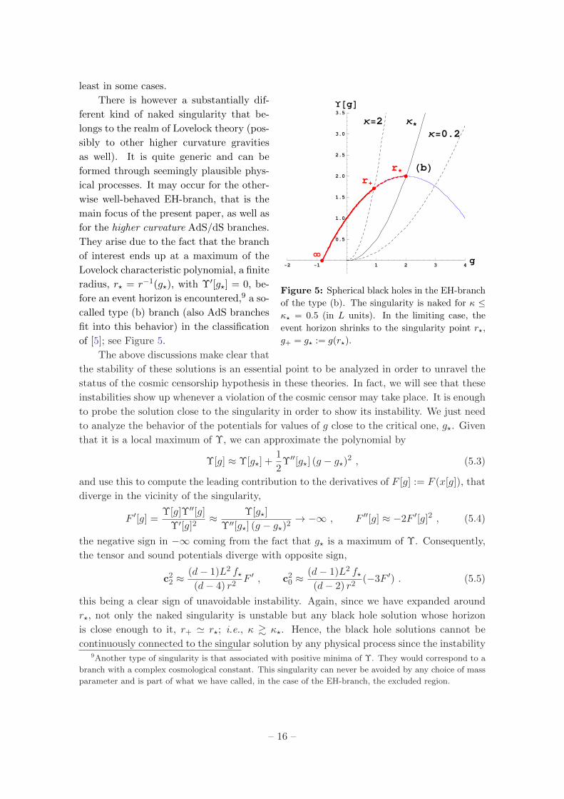
Figure 5: Spherical black holes in the EH-branch

of the type (b). The singularity is naked for κ ≤κ? = 0.5 (in L units). In the limiting case, the

event horizon shrinks to the singularity point r?,

g+ = g? := g(r?).

ferent kind of naked singularity that be-

longs to the realm of Lovelock theory (pos-

sibly to other higher curvature gravities

as well). It is quite generic and can be

formed through seemingly plausible phys-

ical processes. It may occur for the other-

wise well-behaved EH-branch, that is the

main focus of the present paper, as well as

for the higher curvature AdS/dS branches.

They arise due to the fact that the branch

of interest ends up at a maximum of the

Lovelock characteristic polynomial, a finite

radius, r? = r−1(g?), with Υ′[g?] = 0, be-

fore an event horizon is encountered,9 a so-

called type (b) branch (also AdS branches

fit into this behavior) in the classification

of [5]; see Figure 5.

The above discussions make clear that

the stability of these solutions is an essential point to be analyzed in order to unravel the

status of the cosmic censorship hypothesis in these theories. In fact, we will see that these

instabilities show up whenever a violation of the cosmic censor may take place. It is enough

to probe the solution close to the singularity in order to show its instability. We just need

to analyze the behavior of the potentials for values of g close to the critical one, g?. Given

that it is a local maximum of Υ, we can approximate the polynomial by

Υ[g] ≈ Υ[g?] +1

2Υ′′[g?] (g − g?)2 , (5.3)

and use this to compute the leading contribution to the derivatives of F [g] := F (x[g]), that

diverge in the vicinity of the singularity,

F ′[g] =Υ[g]Υ′′[g]

Υ′[g]2≈ Υ[g?]

Υ′′[g?] (g − g?)2→ −∞ , F ′′[g] ≈ −2F ′[g]2 , (5.4)

the negative sign in −∞ coming from the fact that g? is a maximum of Υ. Consequently,

the tensor and sound potentials diverge with opposite sign,

c22 ≈(d− 1)L2 f?

(d− 4) r2F ′ , c20 ≈

(d− 1)L2 f?(d− 2) r2

(−3F ′) . (5.5)

this being a clear sign of unavoidable instability. Again, since we have expanded around

r?, not only the naked singularity is unstable but any black hole solution whose horizon

is close enough to it, r+ ' r?; i.e., κ & κ?. Hence, the black hole solutions cannot be

continuously connected to the singular solution by any physical process since the instability9Another type of singularity is that associated with positive minima of Υ. They would correspond to a

branch with a complex cosmological constant. This singularity can never be avoided by any choice of mass

parameter and is part of what we have called, in the case of the EH-branch, the excluded region.

– 16 –

would inevitably show up with increasing importance before the singularity is attained,

driving the system somewhere else. This is an important point, as long as the threshold

between type (b) black holes and naked singularities is not an extremal solution.

6. Instabilities and black hole evaporation

In our quest to qualitatively understand in which situations Lovelock black holes become

unstable, we have to review the case of evaporating black holes. It is relevant as in previous

analysis the instabilities seemed to appear when the black hole horizon approaches too

much the singularity. This is for instance what happens for type (b) spherical solutions.

As the black hole evaporates it looses mass approaching the critical value (for which the

temperature diverges) in finite time. We have also seen that for type (a) branches in

d = 2K + 1 the black hole solution becomes unstable before reaching the r+ = 0 state,

that in this case is extremal. This process would leave behind a naked singularity, but we

already proved that neither the extremal solution nor the naked singularity can be reached,

the solution becoming unstable as the horizon gets close to the singularity. The black hole

would spend an infinite amount of time to become extremal but just a finite lapse to reach

the instability. Hence, the instability seem to play a role in the evaporation process of

black holes in Lovelock gravities.

The remaining case to be understood is that of type (a) solutions, either belonging to

the EH or dS branches, for dimensions bigger than the critical one, d > 2K + 1. As the

mass of these black hole shrinks to zero, the horizon also contracts approaching the central

singularity. The singularity can never become naked in this case but, still, instabilities show

up before the black hole shrinks to zero size. In [19, 21], Takahashi and Soda observed that

when all possible Lovelock couplings are turned on –the highest one, cK , being positive–,

the instability always shows up, in even and odd dimensions. Here we will generalize that

analysis.

Expanding the tensor and scalar potentials around g →∞ we simply get

c22 ≈(d− 3K − 1)L2 f

K(d− 4) r2, c20 ≈

(d−K − 1)L2 f

K(d− 2) r2. (6.1)

Therefore, any spherical branch under the above conditions will present a tensor instability

in the small mass limit for 2K + 1 < d < 3K + 1, the sound channel being always well

behaved. The d = 3K + 1 is special and we need to go to the following order in the

tensor potential, and whether the black hole is stable or not will depend on the actual

values of (cK−1/cK)2 and cK−2/cK . The Einstein-Hilbert theory is stable in any number

of dimensions.

Summarizing, for generic Lovelock theory we have encountered instabilities at the end

of the evaporation process of any type (a) spherical black hole in dimensions lower than

3K + 1, whereas for type (b) the instability appears for any spacetime dimensionality,

regardless of the asymptotics. The latter dimensionality, d = 3K + 1, has to be considered

more carefully. Whether this instability is pointing towards an inconsistency of the theory

that forces us to constrain K ≤[d−13

]or, else, it can be ascribed to a physically sensible

process taking place during the black hole evaporation has yet to be answered.

– 17 –

7. Final remarks and discussion

Perturbative analysis of exact solutions appears to be an extremely useful tool to get

a deeper understanding of the dynamics of gravity in four and higher dimensions. We

have presented and analyzed the graviton potentials for generic Lovelock gravities in a

particularly simple regime, that of very large momentum and frequency. Still, despite the

simplicity of the adopted approach, the results are general enough to provide some valuable

information about the behavior of black holes in these higher curvature theories.

Lovelock solutions were shown to display several seemingly pathological features, rang-

ing from naked singularities to violations of the third law of thermodynamics or the exis-

tence of discontinuous changes on the radius of multi horizon black holes and, consequently,

also on their associated thermodynamic variables. We have shown that all the puzzling

properties of these solutions are ruled out once their stability is considered. Before any

naked singularity may show up, the corresponding solution becomes unstable, this apply-

ing, to the best of our understanding, both to black holes undergoing any physical process

–accretion of matter or evaporation–, as well as to the collapse of any kind of matter.

Therefore, naked singularities cannot be formed under the evolution of generic initial con-

ditions. The existence of such solutions would require extremely fine-tuned initial data for

the gravitational collapse. Any perturbed set of initial conditions will not end up with the

formation of a naked singularity due to the instability. To the extent we could challenge

it, the cosmic censorship hypothesis seems at work in Lovelock theory. This seems relevant

from the point of view of the uses of Lovelock gravities in the framework of the AdS/CFT

correspondence.

These results provide a new insight into these graviton instabilities, too often taken

as pathological. Much on the contrary, they seem to acquire physical significance and

play an important role, healing Lovelock theory from what otherwise would lead to an

ill-defined behavior. Their analysis is crucial for the understanding of the dynamics of

black holes in Lovelock theory and possibly other theories containing higher powers of the

curvature. In particular, we have shown that Lovelock black holes with spherical symmetry

generically become unstable as they evaporate. In most cases there is a mass gap between

the lightest stable black hole and the corresponding maximally symmetric vacuum. The

instability may be a hint pointing to the existence of new solutions that fill this gap. The

only possibilities we foresee for such hypothetical states are stars made either of regular

matter or gravitational hair.10 In some cases we might need to break spherical symmetry

and provide some angular momentum, as the perturbations considered do.

We have focused mostly on spherical symmetry and the EH-branch in this paper.

The results can be straightforwardly extended to AdS/dS-branches. In the former case,

hyperbolic symmetry is the relevant one, and many results mirror those of spherical black

holes in dS-branches. For hyperbolic AdS-branches the stability of the black hole solutions

provides an upper bound on the gravitational mass coming, again, from maxima of the

characteristic polynomial. The bound should not be of fundamental nature, thus we expect

more massive solutions in the form of hairy black holes, the dressing of the horizon providing

10See [56] for an example of the class of solutions we are referring to.

– 18 –

the extra required energy. The fact that the instability is restricted to a finite (radius)

spacetime region seems to support this hypothesis. This is the region filled by our matter

configuration or, better, our lump of gravitational energy or geon, the rest of the spacetime

remaining untouched. A more detailed analysis is necessary in order to confirm or disprove

this intuition.

Coming back to the spherical case,11 the instability is associated with a particular

value of g, g∗ < g?, above which some of the potentials become negative. The threshold of

the instability is then the mass κ∗ for which the radius of the horizon is r∗ = g−1/2∗ . For

lower values of the mass, we can translate the stability constraints into a bound on the

amount of matter that can be contained in a hypersphere of radius r. For any quantity of

matter contained in such a hypersphere, with mass κ(r), the radius should be bigger than

the would be unstable region for the same mass. For a continuous distribution of matter,

this has to be verified for all values of the radius down to r = 0 so that the configuration

is stable. The equation for the metric function g should be schematically modified [58] in

that case to

Υ[g(r)] =κ(r)

rd−1≤ Υ[g∗] . (7.1)

Of course, to fully address this issue we would need to consider adding matter fields that

in principle may change the stability analysis. The characteristic polynomial plays the role

of an effective density and its value at the threshold of the instability can be interpreted

as the maximal one so that the instability is avoided; see Figure 6.

0 1 2 3 4 5g

0.5

1.0

1.5

2.0

2.5U

Figure 6: Possible resolution of the instabilities in the spherical case for the EH-branch. For

masses below κ∗ (violet curve), the polynomial is interpreted as an effective density with κ(r) being

such that (7.1) holds. This star-like solution is represented by the green curve; it has no event

horizon but smoothly reaches the origin. The type (a) case admits an analogous explanation, since

the behavior of Υ for g > g∗ is irrelevant.

11The hyperbolic case can be discussed quite straightforwardly by mirroring to negative values of g. There

are some subtleties, though, that are beyond the scope of this paper [57].

– 19 –

Even in the event that these configurations are not possible in a Lovelock theory cou-

pled to matter, there is another possible endpoint for gravitational collapse. The collapsing

matter may just disperse again as it is not trapped by any event horizon. In case the sym-

metry is relaxed, the matter will not collapse exactly to one point in such a way that the

density may remain finite through the evolution. Then it may disperse back to infinity or

form some type of bound state. To be conclusive in this point it seems indispensable to

explore the inclusion of matter.

It would be interesting to investigate the status in Lovelock theory of the nonlinear

instability of AdS that was found in General Relativity under small generic perturbations

[59]. Such an instability is triggered by a mode mixing that produces energy diffusion from

low to high frequencies. This mechanism can be understood as a result of the interaction

of geons that end up producing a small black hole [56]. Given the existence of a mass gap

in the Lovelock black hole spectrum, it is natural to wonder whether AdS does not display

turbulent instabilities when small generic perturbations are considered within the higher

curvature dynamics. The only piece of information on this direction that we are aware of

is the analysis of Choptuik’s critical phenomenon [60] in the case of LGB theory without

cosmological constant [61].

A final comment is in order. There is a different notion of instability that may su-

persede that unraveled by perturbative analysis in this paper. Black hole solutions are

subjected to the laws of thermodynamics and, as such, they may become unstable at the

threshold of a (for instance, Hawking-Page) phase transition. In a thermal bath, it has been

recently shown, indeed, that Lovelock theory admits generalized phase transitions allowing

for jumps between the different branches [62, 63]. This phenomenon further enriches the

rules of the game and make it cumbersome and interesting to reinstate a basic question

with which we would like to finish the paper: Are higher curvature gravities like Lovelock

theory fully consistent?

Acknowledgements

We wish to thank Oscar Dias, Ricardo Monteiro and Jorge Santos for useful discussions.

This work was supported in part by MICINN and FEDER (grant FPA2011-22594), by

Xunta de Galicia (Consellerıa de Educacion and grant PGIDIT10PXIB206075PR), and

by the Spanish Consolider-Ingenio 2010 Programme CPAN (CSD2007-00042). We would

like to thank the Universities of Buenos Aires and Andres Bello, as well as the Institute

for Advanced Study and the Benasque Centre for Science Pedro Pascual for hospitality

during part of this project. X.O.C. is thankful to the Front of Galician-speaking Scientists

for encouragement. The Centro de Estudios Cientıficos (CECs) is funded by the Chilean

Government through the Centers of Excellence Base Financing Program of Conicyt.

References

[1] D. Lovelock, “The Einstein tensor and its generalizations,” J. Math. Phys. 12 (1971) 498.

[2] C. Lanczos, “A Remarkable property of the Riemann-Christoffel tensor in four dimensions,”

Annals Math. 39 (1938) 842.

– 20 –

[3] J. D. Edelstein, “Lovelock theory, black holes and holography,” arXiv:1303.6213

[4] X. O. Camanho, J. D. Edelstein and J. M. Sanchez de Santos, “Lovelock theory and the

AdS/CFT correspondence,” to appear.

[5] X. O. Camanho and J. D. Edelstein, “A Lovelock black hole bestiary,” Class. Quant. Grav.

30 (2013) 035009; arXiv:1103.3669 [hep-th].

[6] C. Charmousis, “Higher order gravity theories and their black hole solutions,” Lect. Notes

Phys. 769 (2009) 299; arXiv:0805.0568 [gr-qc]].

[7] C. Garraffo and G. Giribet, “The Lovelock Black Holes,” Mod. Phys. Lett. A 23 (2008) 1801;

arXiv:0805.3575 [gr-qc]].

[8] T. Regge and J. A. Wheeler, “Stability of a Schwarzschild singularity,” Phys. Rev. 108

(1957) 1063.

[9] F. J. Zerilli, “Effective potential for even-parity Regge-Wheeler gravitational perturbation

equations,” Phys. Rev. Lett. 24 (1970) 737.

[10] S. Teukolsky, “Rotating black holes: Separable wave equations for gravitational and

electromagnetic perturbations,” Phys. Rev. Lett. 29 (1972) 1114.

[11] A. Ishibashi and H. Kodama, “Perturbations and stability of static black holes in higher

dimensions,” Prog. Theor. Phys. Supplement 189 (2011) 165; arXiv:1103.6148 [hep-th].

[12] G. Dotti and R. J. Gleiser, “Gravitational instability of Einstein-Gauss-Bonnet black holes

under tensor mode perturbations,” Class. Quant. Grav. 22 (2005) L1; arXiv:0409005

[gr-qc].

[13] G. Dotti and R. J. Gleiser, “Linear stability of Einstein-Gauss-Bonnet static spacetimes.

Part. I: Tensor perturbations,” Phys. Rev. D 72 (2005) 044018; arXiv:gr-qc/0503117.

[14] R. Gleiser and G. Dotti, “Linear stability of Einstein-Gauss-Bonnet static spacetimes. Part II:

Vector and scalar perturbations,” Phys. Rev. D 72 (2005) 124002; arXiv:0510069 [gr-qc].

[15] I. P. Neupane, “Thermodynamic and gravitational instability on hyperbolic spaces,” Phys.

Rev. D 69 (2004) 084011; arXiv:0302132 [hep-th].

[16] M. Beroiz, G. Dotti and R. J. Gleiser, “Gravitational instability of static spherically

symmetric Einstein-Gauss-Bonnet black holes in five and six dimensions,” Phys. Rev. D 76

(2007) 024012; arXiv:hep-th/0703074.

[17] R. Konoplya and A. Zhidenko, “(In)stability of D-dimensional black holes in Gauss-Bonnet

theory,” Phys. Rev. D 77 (2008) 104004; arXiv:0802.0267.

[18] T. Takahashi and J. Soda, “Stability of Lovelock black holes under tensor perturbations,”

Phys. Rev. D 79 (2009) 104025; arXiv:0902.2921 [gr-qc].

[19] T. Takahashi and J. Soda, “Instability of small Lovelock black holes in even dimensions,”

Phys. Rev. D 80 (2009) 104021; arXiv:0907.0556.

[20] T. Takahashi and J. Soda, “Master equations for gravitational perturbations of static

Lovelock black holes in higher dimensions,” Prog. Theor. Phys. 124 (2010) 911;

arXiv:1008.1385 [gr-qc].

[21] T. Takahashi and J. Soda, “Catastrophic instability of small Lovelock black holes,” Prog.

Theor. Phys. 124 (2010) 711; arXiv:1008.1618 [gr-qc].

– 21 –

[22] T. Takahashi and J. Soda, “Pathologies in Lovelock AdS Black Branes and AdS/CFT,”

Class. Quant. Grav.. 29 (2012) 035008; arXiv:1108.5041 [hep-th].

[23] D. G. Boulware and S. Deser, “String Generated Gravity Models,” Phys. Rev. Lett. 55

(1985) 2656.

[24] X. O. Camanho, J. D. Edelstein and M. F. Paulos, “Lovelock theories, holography and the

fate of the viscosity bound,” JHEP 1105 (2011) 127; arXiv:1010.1682 [hep-th].

[25] R. Penrose, “Gravitational collapse: the role of General Relativity,” Riv. Nuovo Cim. 1

(1969) 252 [Gen. Rel. Grav. 34 (2002) 1141].

[26] H. Maeda, “Effects of Gauss-Bonnet terms on final fate of gravitational collapse,” Class.

Quant. Grav. 23 (2006) 2155; arXiv:gr-qc/0504028.

[27] H. Maeda, “Final fate of spherically symmetric gravitational collapse of a dust cloud in

Einstein-Gauss-Bonnet gravity,” Phys. Rev. D 73 (2006) 104004; arXiv:gr-qc/0602109.

[28] M. Nozawa and H. Maeda, “Effects of Lovelock terms on the final fate of gravitational

collapse: Analysis in dimensionally continued gravity,” Class. Quant. Grav. 23 (2006) 1779;

arXiv:gr-qc/0510070.

[29] M. H. Dehghani and N. Farhangkhah, “Asymptotically flat radiating solutions in third order

Lovelock gravity,” Phys. Rev. D 78 (2008) 064015; arXiv:0806.1426 [gr-qc].

[30] P. Rudra, R. Biswas and U. Debnath, “Gravitational collapse in generalized Vaidya

spacetime for Lovelock gravity theory,” Astrophys. Space Sci. 335 (2011) 505;

arXiv:1101.0386 [gr-qc].

[31] S. Ohashi, T. Shiromizu and S. Jhingan, “Spherical collapse of inhomogeneous dust cloud in

the Lovelock theory,” Phys. Rev. D 84 (2011) 024021; arXiv:1103.3826 [gr-qc].

[32] K. Zhou, Z. -Y. Yang, D. -C. Zou and R. -H. Yue, “Spherically symmetric gravitational

collapse of a dust cloud in third order Lovelock gravity,” Int. J. Mod. Phys. D 20 (2011)

2317; arXiv:1107.2730 [gr-qc].

[33] S. Ohashi, T. Shiromizu and S. Jhingan, “Gravitational collapse of charged dust cloud in the

Lovelock gravity,” Phys. Rev. D 86 (2012) 044008; arXiv:1205.5363 [gr-qc].

[34] R. Goswami and P. S. Joshi, “Cosmic censorship in higher dimensions,” Phys. Rev. D 69

(2004) 104002; arXiv:gr-qc/0405049.

[35] P. S. Joshi, “Gravitational collapse and spacetime singularities,” Cambridge University Press,

Cambridge, UK, 2007.

[36] R. Zegers, “Birkhoff’s theorem in Lovelock gravity,” J. Math. Phys. 46 (2005) 072502;

arXiv:gr-qc/0505016.

[37] X. O. Camanho and J. D. Edelstein, “Causality in AdS/CFT and Lovelock theory,” JHEP

1006 (2010) 099; arXiv:0912.1944 [hep-th].

[38] J. T. Wheeler, “Symmetric solutions to the Gauss-Bonnet extended Einstein equations,”

Nucl. Phys. B 268 (1986) 737.

[39] J. T. Wheeler, “Symmetric solutions to the maximally Gauss-Bonnet extended Einstein

equations,” Nucl. Phys. B 273 (1986) 732.

[40] R. Aros, R. Troncoso and J. Zanelli, “Black holes with topologically nontrivial AdS

asymptotics,” Phys. Rev. D 63 (2001) 084015; arXiv:hep-th/0011097.

– 22 –

[41] G. Policastro, D. T. Son and A. O. Starinets, “From AdS/CFT correspondence to

hydrodynamics,” JHEP 09 (2002) 043; arXiv:hep-th/0205052.

[42] D. Wiltshire, “Spherically symmetric solutions of Einstein-Maxwell theory with a

Gauss-Bonnet term,” Phys. Lett. B 169 (1986) 36.

[43] D. Wiltshire, “Black holes in string-generated gravity models,” Phys. Rev. D 38 (1988) 2445.

[44] A. Buchel, J. Escobedo, R. C. Myers, M. F. Paulos, A. Sinha and M. Smolkin, “Holographic

GB gravity in arbitrary dimensions,” JHEP 1003 (2010) 111; arXiv:0911.4257 [hep-th].

[45] R. C. Myers, A. O. Starinets and R. M. Thomson, “Holographic spectral functions and

diffusion constants for fundamental matter,” JHEP 0711 (2007) 091; arXiv:0706.0162

[hep-th].

[46] M. Brigante, H. Liu, R. C. Myers, S. Shenker and S. Yaida, “The viscosity bound and

causality violation,” Phys. Rev. Lett. 100 (2008) 191601; arXiv:0802.3318 [hep-th].

[47] J. de Boer, M. Kulaxizi and A. Parnachev, “AdS7/CFT6, Gauss-Bonnet gravity, and

viscosity bound,” JHEP 1003 (2010) 087; arXiv:0910.5347 [hep-th].

[48] X. O. Camanho and J. D. Edelstein, “Causality constraints in AdS/CFT from conformal

collider physics and Gauss-Bonnet gravity,” JHEP 1004 (2010) 007; arXiv:0911.3160

[hep-th].

[49] J. de Boer, M. Kulaxizi and A. Parnachev, “Holographic Lovelock gravities and black holes,”

JHEP 1006 (2010) 008; arXiv:0912.1877 [hep-th].

[50] J. Zanelli, “Lecture notes on Chern-Simons (super-)gravities,” arXiv:0502193 [hep-th].

[51] M. Banados, C. Teitelboim and J. Zanelli, “Dimensionally continued black holes,” Phys. Rev.

D 49 (1994) 975; arXiv:gr-qc/9307033.

[52] J. Crisostomo, R. Troncoso and J. Zanelli, “Black hole scan,” Phys. Rev. D 62 (2000)

084013; arXiv:hep-th/0003271.

[53] P. R. Anderson, W. A. Hiscock, and D. J. Loranz, “Semiclassical stability of the extreme

Reissner-Nordstrom black hole,” Phys. Rev. Lett. 74 (1995) 4365; arXiv:gr-qc/9504019.

[54] D. Marolf, “The dangers of extremes,” Gen. Rel. Grav. 42 (2010) 2337; arXiv:1005.2999

[gr-qc].

[55] L. Vanzo, “Black holes with unusual topology,” Phys. Rev. D 56 (1997) 6475;

arXiv:gr-qc/9705004.

[56] O. J. C. Dias, G. T. Horowitz and J. E. Santos, “Gravitational turbulent instability of

anti-de Sitter space,” Class. Quant. Grav. 29 (2012) 194002; arXiv:1109.1825 [hep-th].

[57] X. O. Camanho, “Lovelock gravity, black holes and holography,” PhD thesis, to appear.

[58] M. F. Paulos, “Holographic phase space: c-functions and black holes as renormalization

group flows,” JHEP 1105 (2011) 043; arXiv:1101.5993 [hep-th].

[59] P. Bizon and A. Rostworowski, “On weakly turbulent instability of anti-de Sitter space,”

Phys. Rev. Lett. 107 (2011) 031102; arXiv:1104.3702 [gr-qc].

[60] M. W. Choptuik, “Universality and scaling in gravitational collapse of a massless scalar field,

Phys. Rev. Lett. 70 (1993) 9;

– 23 –

[61] S. Golod and T. Piran, “Choptuik’s critical phenomenon in Einstein-Gauss-Bonnet gravity,

Phys. Rev. D 85 (2012) 104015: arXiv:1201.6384 [gr-qc].

[62] X. O. Camanho, J. D. Edelstein, G. Giribet, and A. Gomberoff, “New type of phase transition

in gravitational theories,” Phys. Rev. D 86 (2012) 124048; arXiv:1204.6737 [hep-th].

[63] X. O. Camanho, J. D. Edelstein, G. Giribet, and A. Gomberoff, “Generalized phase

transition in Lovelock theory,” to appear.

– 24 –