arX

iv:0

708.

2816

v1 [

astr

o-ph

] 2

1 A

ug 2

007

Testing Isotropy of

Cosmic Microwave Background Radiation

Pramoda Kumar Samal1, Rajib Saha1 Pankaj Jain1

John P. Ralston2

February 1, 2008

1Department of Physics, Indian Institute of Technology, Kanpur, U.P,208016, India

2Department of Physics & Astronomy, University of Kansas, Lawrence, KS66045, USA

Abstract

We introduce new symmetry-based methods to test for isotropyin cosmic microwave background radiation. Each angular multipoleis factored into unique products of power eigenvectors, related mul-tipoles and singular values that provide 2 new rotationally invariantmeasures mode by mode. The power entropy and directional entropy

are new tests of randomness that are independent of the usual CMBpower. Simulated galactic plane contamination is readily identified,and the new procedures mesh perfectly with linear transformationsemployed for windowed-sky analysis. The ILC -WMAP data mapsshow 7 axes well aligned with one another and the direction Virgo.Parameter free statistics find 12 independent cases of extraordinaryaxial alignment, low power entropy, or both having 5% probability orlower in an isotropic distribution. Isotropy of the ILC maps is ruledout to confidence levels of better than 99.9%, whether or not coinci-dences with other puzzles coming from the Virgo axis are included.Our work shows that anisotropy is not confined to the low l region,but extends over a much larger l range.

Keywords: cosmic microwave background, methods:data analysis, meth-ods:statistical

1

1 Introduction

Studies of the cosmic microwave background (CMB) were long posed in termsof the temperature power spectrum. The power spectrum is invariant underrotations, and by itself cannot in principle test the basic postulate that theradiation field should be statistically isotropic. The availability of high qual-ity data from WMAP (Hinshaw et al 2003, 2007) has allowed isotropy to beexamined critically, and with surprising outcomes.

A long-standing question exists in the unexpected size of low-l multipoles.Interpretation of this is stalemated by inherent uncertainties of fluctuationscalled cosmic variance. Directional effects are much more decisive, becausethey confront a symmetry. de Oliveira-Costa, et al (2004) constructed anaxial statistic for which they found modest statistical significance in multi-poles for l = 2, 3 being rather well aligned. The fact that the dipole (l = 1)also aligns very closely with the multipoles l = 2, 3 was later highlightedby Ralston and Jain (2004) and Schwarz et al (2004). When the dipole isinterpreted to be due to our proper motion, it has sometimes been excludedas having “no cosmological significance.” However there are many physi-cal mechanisms which can correlate CMB observations with galactic motion.There are good reasons not to exclude it, and the correlation of all three mul-tipoles significantly aligned with the constellation Virgo is quite inconsistentwith chance.

Subsequently there have been a large number of studies (Eriksen et al

2004, Katz and Weeks 2004, Bielewicz et al 2004, Bielewicz et al 2005, Prunetet al 2005, Copi et al 2006, de Oliveira-Costa and Tegmark 2006, Wiaux et

al 2006, Bernui et al 2006, Freeman et al 2006, Magueijo and Sorkin 2007,Bernui et al 2007, Copi et al 2007, Helling et al 2007, Land and Magueijo2007) which claim the CMB is not consistent with isotropy. Several physicalexplanations for the observed anisotropy have been put forward (Armendariz-Picon 2004, Moffat 2005, Gordon et al 2005, Vale 2005, Abramo et al 2006,Land and Magueijo 2006, Rakic et al 2006 Gumrukcuoglu et al 2006, Inoueand Silk 2006, Rodrigues 2007, Naselsky et al 2007, Campanelli et al 2007).It has also been suggested that the anisotropy may be due to foregroundcontamination (Slosar and Seljak 2004). Land and Magueijo (2005) findevidence that the detected anisotropy has positive mirror parity. Meanwhilesome studies find no inconsistency ( Hajian et al 2004, Hajian and Souradeep2006, Donoghue and Donoghue 2005). There have also been several studiesof the primordial perturbations (Koivisto and Mota 2006, Battye and Moss

2

2006, Armendariz-Picon 2006, Pereira et al 2007, Gumrukcuoglu et al 2007)and inflation (Hunt and Sarkar 2004, Buniy et al 2006) in an anisotropicuniverse.

It is clearly necessary to explore new observables to determine whetheranisotropy may be signs of physics beyond the standard paradigm. Herewe develop new methods to test CMB data for isotropy. The new tests arepossible because there exist many more invariant and vector-valued quantitiesthan commonly examined. As conventional, the temperature distribution∆T (n) is expanded in terms of the spherical harmonics, defining ∆T (n) =∑

lm almYlm(n), where n is a unit vector on the sky. The assumption ofstatistical isotropy is the statement that the ensemble average is given by

< alma∗l′m′ >= Clδll′δmm′ . (1)

As a consequence all tensors formed from products of alm must be isotropic.We concentrate on the second rank tensors that can be formed, which includethe isotropic power Cl δij and the power tensor Aij(l). They are defined by

A(l) δij =1

2l + 1

∑

mm′

a∗lmδijδmm′alm′ ;

Aij(l) =1

l(l + 1)

∑

mm′

a∗lm( JiJj )mm′alm′ . (2)

Here Ji are the angular momentum operators in representation l for Cartesianindices i = 1...3. From Eq. 1 statistical isotropy predicts the ensembleaverages

< A >= Cl;

< Aij(l) >= Clδij . (3)

Giving attention to the power tensor represents a modest step towardsexamining the data more thoroughly. Consider the region of 0 < l < 300,which includes the acclaimed peak in plots of l(l + 1)Cl. There are 299 datapoints from 2 ≤ l ≤ 300 but the information makes a smooth curve, onethat can be fit with 3 or 4 parameters. The existence of an acoustic peakis useful but only the beginning of tests. Each alm has 2l + 1 components,and the remaining 90,298 numbers, measured at great effort and considerablepublic expense, are never examined with the power spectrum. One reasoncomes from early tradition when data was poor. There also appears to be a

3

widespread but false belief that the power spectrum is the only rotationallyinvariant quantity.

The approach of Copi et al (2007) consists of factoring the spherical har-monics expansion into products of vector-valued terms. All spherical har-monics can be developed from traceless symmetric polynomials of vectorproducts. There are 2l + 1 real freedoms in multipoles of given l. Each mu-tipole can be factored into l unit vectors, each with 2 freedoms, making 2lterms (Weeks 2004, Katz and Weeks 2004). Finally there is one overall powercoefficient. The analysis of 50 vectors for l = 50 (say) is inherently compli-cated, and complicated further by discovery that Maxwell-multipole vectorsof isotropic data are kinematically correlated to “repel” one another. Dennis(2005) discusses this and even solves the 2-point correlation analytically.

Factoring into products of vectors is natural for tensors of rank 2. Whenwe consider rank-2 tensors, we realize they have more than one invarianteigenvalue, so that the CMB power cannot even describe the quadrupolecomponent. Tensors of rank higher than 2 have many types of invariants.One complication in finding them is the absence of a unique canonical formfor high-rank tensors (da Silva and Lim 2006). Another technical obstacleis to obtain the invariants using quadratic functions of the data, which arestatistically robust.

The technical problems are solved here with a procedure exploiting aninvariant canonical form where unique and preferred vectors are factored fromeach multipole. The fact this can be done is both obvious from symmetry andsystematic via Clebsch-Gordan series. It is a particular linear transformation

of the alm that leads to the power tensor Aij as quadratic form. When ourprocedure is applied to WMAP data there are numerous new invariants andseveral new signals of anisotropy.

We had two distinct motivations in beginning our study:

• Isotropy is a well-defined statistical data question that does not needany physical hypothesis to be motivated. Physical hypotheses are bestcharacterized and tested through their symmetries. No free parametersare used in expressing isotropy, which can be confirmed or ruled outindependent of the parameterization of model predictions. All of thenew tests in this paper are also parameter-free. Isotropy of the CMB isalso a separate issue from isotropy of other observables in the universe.This is because the CMB contains both information on formation ininteraction with matter, and information on the propagation of light

since the era of decoupling. By separating tests of isotropy of the CMBwe maintain an orderly process of testing larger issues in cosmology.

• Anisotropy of the CMB may be a signal of physics beyond electro-dynamics and gravity. The interaction of light with an anisotropicaxion-like condensate, or its conversion into weakly interacting parti-cles, may give anisotropic signatures without disturbing the large scaledistribution of matter.

Interestingly, there is a long history of “Virgo alignment” of electro-magnetic propagation effects which cannot be explained by any knownmedia of conventional physics. Propagation of radiation in the sub-GHz region of radio telescopes, the 20-90 GHz region of CMB studies,and the optical region all reveal anisotropic effects. Many years agoBirch (1982) observed that the offsets of sub-GHz linear polarizationsrelative to radio galaxy axes were not distributed isotropically. Thestatistical significance of Birch’s signal was confirmed by Kendall andYoung (1984) and a statistic used by Bietenholz and Kronberg (1984),but generally rejected nonetheless. The redshift-dependent signal foundby Nodland and Ralston (1997) was also generally dismissed. Rejectionwas based on not finding correlation in statistics believed to test for thesame signals. Yet one must be sure the same tests were really made.Paradoxes were finally resolved by classification under parity. Statis-tics finding no signal test for even parity distribution with no senseof twist, while those statistics of odd parity consistently show signalsof high statistical significance. Subsequent analysis (Jain and Ralston1999, Jain and Sarala, 2006) has found a robust axial relationship ofodd parity character and aligned with Virgo.

Until recently these explorations of anisotropy were conducted in the ra-dio regime, which might indicate a conventional explanation in plasmaelectrodynamics. The discovery of optical frequency polarization cor-relations (Hutsemekers (1998), Hutsemekers and Lamy (2001)) fromcosmologically distant QSO’s is extraordinary. The optical correlationsagain generate an axis aligned with Virgo (Ralston and Jain 2004). Thecoincidence of 5 closely aligned axes coming from 3 distinct frequencydomains makes an exceptional mystery that merits further study.

In this paper we make no attempt at physical explanation of anisotropy.Our new methods provide two independent new roads for data analysis. Or-

5

der by order for each l ≥ 2 there exist three rotationally invariant eigen-values of Aij(l). The sum of three eigenvalues reproduce the usual powerCl. Meanwhile two independent combinations are new invariants. For theregion of 2 ≤ l ≤ 50, say, we have 98 new invariants never examined be-fore. The isotropic CMB model predicts that all three eigenvalues shouldbe degenerate and equal to Cl/3, up to fluctuations. We test this predictionby introducing the power entropy of Aij. Inspired by quantum statisticalmechanics, the power entropy is a stable and bounded measure of the ran-domness of eigenvalues of matrix Aij. The entropy of the data turns out notto be consistent with the conventional CMB prediction. Next we examine theeigenvectors of Aij . The eigenvectors are independent covariant quantities.Under the isotropic prediction they should be randomly oriented. For therange of 2 ≤ l ≤ 50 there are 98 independent eigenvectors, and 49 “principal”eigenvectors associated with the largest eigenvalues. The largest eigenvaluemakes the largest contribution to the total power and gives an objective rea-son to be singled out. Statistical measures of the alignment of eigenvectorsdo not happen to support the random isotropic expectations. Instead 6 axesobtained from the range 2 ≤ l ≤ 50 are found to be well aligned with thedipole or Virgo axis, each case having independent probability of less than5%.

1.1 Outline of the Paper

Transformation properties and signal processing of alm are encoded by linearoperations. To take advantage we first introduce ψk

m, which is the uniquelinear transformation of alm that divides each l-multiplet into direct productsof irreducible representations with vectors. We relate ψk

m to the power tensor,and study the distribution of invariants in the ILC map.

Complementary to these studies are comparisons with “masked-sky” powerspectra, evaluated with a window-function blocking out a particular angularregion. Our linear transformations are made to mesh perfectly with the lin-ear operations of window functions and subtractions. In studies we report,we sometimes masked out the plane of the galaxy, and divided the remainderinto two “top” and “bottom” regions. We study statistics of the regions asgiven, and also the statistics of full-sky maps they predict under standardprocedures. There are several reasons for the masked sky studies. First, wecan both study top/bottom asymmetries as a simple probe of isotropy in-

cluding the galactic plane. We also study “cone-masks” which retain only a

6

region subtended by cones at high galactic latitudes, reducing the importanceof galactic plane contamination. Finally we make simulations of galactic con-tamination and show that our new methods readily detect contamination andfind its angular location. The ILC data maps turn out to show significantanisotropy that cannot be attributed to galactic foregrounds.

In the following section we describe the new methods. Applications todata follow. Not surprisingly, the power tensor method is generally moresensitive to anisotropy than power spectrum methods. Yet power spectrummethods find similar signals of anisotropy. This is significant because the twoapproaches are statistically independent - nothing about the power spectrumis used in the new approach. Almost all of our studies develop new informa-tion that by construction is independent of the usual CMB power Cl.

The reliability of CMB maps is not under our control and certainly opento debate. The observers of the ILC team present maps claimed to havesystematic errors equal to or smaller than cosmic variance. For this reasonwe don’t discuss systematic errors. Our results are quantified using statisticalerrors based on Monte Carlo simulations with random realizations in placeof the alm.

2 Covariant Frames and Invariant Singular

Values

In this Section we use Dirac notation with

alm = 〈l, m | a(l)〉 .

(There should be no confusion with ensemble averages.) The states |lm〉 are

eigenvectors of angular momentum ~Jz and ~J2 with eigenvalues m, l(l + 1).The temperature measurements are real valued, which produces a constraintin the usual basis convention:

alm = (−1)m a∗l−m

Although the phase conventions standardize the alm they have no effect onanything we report.

Besides simplicity, the power tensor is well motivated on rotational sym-metry grounds. Each multipole alm → |a(l)〉 represents a geometrical object

7

visualized as a complicated beach-ball. “Holding by hand” the object forinspection, make a small rotation by angle ~θ, under which

|a(l)〉 → |a(l)〉′ = |a(l)〉 + |δa(l)〉 ;

|δa(l)〉 = −i~θ · ~J |a(l)〉 .

Under what axes does the rotation make the most difference ? Compute theHessian of the change,

∂2

∂θi∂θj

〈δa(l) | δa(l)〉 = 〈a(l)| J iJ j |a(l)〉

= Aij

By Rayleigh-Ritz variation, the maximum rotation is developed along theeigenvectors of Aij , which are natural principal axes of the alm as objectsorder by order in l.

It is convenient to define a linear map or “wave function” ψkm(l) (Ralston

and Jain 2004) we call “vector factorization:”

ψkm(l) =

1√

l(l + 1)〈l, m|Jk|a(l)〉. (4)

The purpose of this transformation is to extract (algebraically divide out)a vector (spin -1) quantity from each representation of spin−l, so each canbe covariantly compared across different l. Inserting a complete set of statesgives

ψkm(l) =

1√

l(l + 1)

l∑

m′=−l

〈l, m|Jk|l, m′〉〈l, m′|a(l)〉

=

l∑

m′=−l

Γkmm′ alm′ (5)

where

Γkmm′ =

1√

l(l + 1)〈l, m|Jk|l, m′〉 (6)

Under rotations each index of ψkm rotates by its representation R(j), namely

ψkm → ψk′

m = Rkk′

(1)Rmm′(l)ψkm. (7)

8

The transformation a→ ψ is invertible. The inverse relation can be written

alm =∑

km′

Γmm′

k ψkm ,

where

Γmm′

k =1

√

l(l + 1)〈l, m|Jk|l, m′〉,

= Γkmm′ .

Upon rotating ψ by the rule of Eq. 7, then

alm → a′lm = Γmm′

k Rkk′

(1)Rmm′(l)ψkm,

= Rmm′(l)alm′ .

The standard power spectrum invariant is one of the invariants producedfrom ψk

m: it is∑

mk

ψkmψ

k∗m =

∑

m

alma∗lm.

Mathematically ψ represents the multiplet a as a unique sum of outerproducts of vectors eα (spin-1 representation) with representations uα ofspin−l. The terms are obtained by the singular value decomposition (SVD),

ψkm(l) =

3∑

α=1

eαkΛαuα∗

m (8)

Here and in subsequent equations we suppress label l when it is obvious. TheAppendix discusses factorization in general terms of a Clebsh-Gordan series.

The singular values Λα are invariants under rotations on the indices kand m. (Indeed they are invariants under the even higher symmetry ofindependent SO(3) × SO(3) rotations.) The various factors are constructedby diagonalizing the 3 × 3 Hermitian matrices

(ψψ†)kk′

(l) =∑

m

ψkm(l)ψk′∗

m (l),

=∑

α

eαi (Λα)2eα∗

i ; (9)

(ψ†ψ)mm′(l) =∑

k

ψk∗m (l)ψk

m′(l),

=∑

α

uαm(Λα)2uα∗

m′.

9

Since they are the eigenvectors of Hermitian matrices the eα and uα aregenerally orthogonal, except for exceptional degeneracies, and normalized to

∑

k

eα∗k eβ

k = δαβ ;

∑

m

uα∗m u

βm = δαβ.

Since (Λα)2 are the eigenvalues of Hermitian matrices they are real and pos-itive, with Λα > 0 defining the sign convention for eα. Since alm are real, wealso have eα real valued.

The set of three orthogonal eα defines the “frame vectors”, which makea preferred frame for the vector components of ψ. In that preferred frameand the frame of three uα, the matrix ψk

m is diagonal with three invariantsingular values Λα. We will call Λαδαβ the “SV matrix”, SV standing forsingular values.

2.1 Isotropy

The relation of ψkm to the power tensor Aij is simple algebra. We have

Aij(l) =1

l(l + 1)tr( J i |a(l)〉 〈a(l)| J j),

where tr is the trace.Then

Aij(l) =∑

m

ψim(l)ψj∗

m (l),

=∑

α

eαi (l)(Λα(l))2eα∗

j (l),

which is just Eq. 9. Isotropy holds that the eigenvectors eα must be dis-tributed isotropically on the sky and that the eigenvalues Λα are randomvariables concentrated at

√

Cl/3. In terms of the ψkm factors, Eq. 1 predicts

< ψkm(l)ψk′∗

m′ (l′) >=Cl

3δll′δmm′δkk′

. (10)

Eq. 10 can be contrasted with the correlations of Maxwell-multipolevectors developed by dividing multipoles into products of vectors. Those

10

vectors have not been organized into irreducible representations nor classi-fied in invariant terms of importance, and they do not have an uncorrelateddistribution (Dennis 2005). An advantage of using our ψk

m representations isthat isotropy transforms to isotropy without annoying Jacobian factors.

Here is how to interpret the factors. The highest possible degree ofanisotropy produces one singular value equal to the total power, and twoothers that vanish. The corresponding alm components can be written as theproduct of one vector e(1) and one multiplet u(1). We will call this special sit-uation a “pure state.” This has a very simple realization for the quadrupolecase l = 2. Any quadrupole is equivalent to a symmetric 3 × 3 matrix madefrom sums of products of 3-vectors. A generic symmetric matrix has 3 realand unequal eigenvalues. If two eigenvalues vanish then the matrix is theouter product of a unique vector, a pure state. Conversely, if all eigenval-ues are degenerate, the matrix is a (trace subtracted) multiple of the unitmatrix, equivalent to the sum of outer products of three frame vectors bycompleteness, 1 =

∑

α |eα〉 〈eα| , which is the isotropic prediction.

2.2 Tensor Power Entropy

The isotropy hypothesis that the SV matrix should be√

Cl/3 times the unitmatrix can be tested in several different invariant ways.

The information entropy or simply power entropy of the power tensorcomes by recognizing that ρkk′

= (ψψ†)kk′

is proportional to a density matrixon 3-space. The proportionality constant is the overall power. Removing itproduces a normalized form

ρkk′

=(ψψ†)kk′

∑

j (ψψ†)jj. (11)

Von Neumann (1932) found the entropy S of normalized Hermitian matrixρ to be

S = −tr( ρ log( ρ ) ), (12)

=∑

α

(Λα)2log((Λα)2),

0 ≤ S ≤ log(3).

Here (Λα)2 are normalized to sum to one, again removing the overall power

11

from discussion:

(Λα)2 =(Λα)2

∑

α′ (Λα′)2(13)

This normalizes tr(ρ) = 1.The entropy is unique in being invariant, extensive, positive, additive for

independent subsystems, and zero for pure states. A density matrix withno information is a multiple of the unit matrix, and has entropy equallingthe log of its dimension. Very simply Siso → log(3) is the isotropic CMBprediction. Low entropy compared to isotropy is a measure of concentrationof power along one or another eigenvector of ρ. In the present context purestates have all the power in one singular value, define one single directionaleigenvector, and have power entropy Spure → 0.

2.3 Power Alignments Across l-Classes

Our methods allow us to explore the alignment of power tensors betweendifferent l-classes.

One of the most interesting tests concerns the “principal axis e(l)”, whichmeans the eigenvector with the largest eigenvalue for each l. From Eq. 10 theset of all principal frame vectors should be a symmetrical ball in the isotropicprediction. If the data is anisotropic a bundle of vectors may lie along anaxis or in a preferred plane. It is important to remember that the sign ofeigenvectors is meaningless, and determined by algorithms assigning signsin computer code. Thus the “average” eigenvector is not a good statistic.Tensor products are the natural probe of a collection. For statistical studieswe construct a matrix X defined by

Xij(lmax) =lmax∑

l=2

elie

lj . (14)

The eigenvalues of X are a probe of the shape of the bundle collected from2 ≤ l ≤ lmax. We probe the isotropy of the collection with the directional

entropy SX computed using Eq. 12 and X → ρX . The directional entropydoes not use the singular values of the CMB data, and is independent of thepower entropy. Confirmation of isotropy comes if SX ∼ log(3) up to randomfluctuations. A signal of anisotropy would be an unusually low value of SX

compared to log(3).

12

2.3.1 Traceless Power Tensor

We also compare alignments using a statistic that includes the weighting bysingular values. For this purpose we define the traceless power tensor Bij ,

Bij(l) = Aij(l) − 1

3tr(A(l) )δij.

The eigenvectors of B are the same as A, but the value of the total powerhas been removed. To compare two angular momenta classes we examine thecorrelation

Y (l, l′) =tr(B(l)B(l′) )

√

tr(B(l)B(l) )√

tr(B(l′)B(l′) ). (15)

In the isotropic uncorrelated model Y (l, l′) should be proportional to δll′.

3 Full Sky Studies

The WMAP-ILC team developed a foreground cleaned temperature anisotropymap using a method described as Internal Linear Combination (ILC). Theprocess combines data from 5 bands of frequencies 23, 33, 41, 61, and 91GHz. While there also exist several other cleaning procedures that are inter-esting to compare (Tegmark et al 2003, Saha et al 2006, Eriksen et al 2007),our main focus lies on the ILC map.

According to Hinshaw et al (2007) the ILC map is known to becomedominated by statistical instrumental noise for l & 400. Errors on the alm

come from several sources. Systematic errors may occur from inappropri-ate foreground subtractions. Ambiguities in combining frequency bands alsocontribute. The range 2 ≤ l ≤ 50 is considered to be reliable under state-ments that statistical and systematic errors lie within ranges typical of cosmicvariance. We restrict our studies to this range.

Fig. 1 shows the normalized eigenvalues Λα, with a dashed line for theisotropic prediction Λα = Cl/

√3. The normalization is

∑

α (Λα)2 = 1. Thepower entropy Sfull−sky(l) mode by mode in l for the ILC map is shown inFig. 2. By Monte Carlo simulations we find that the points l= 6, 16, 17, 30,34, 40 appear to be statistically unlikely.

We generated random alm and derived the power entropy using 10,000realizations of CMB maps. In our procedure real al0 values were drawn from

13

0

0.2

0.4

0.6

0.8

1

0 10 20 30 40 50

~ Λα

lFigure 1: Normalized singular values versus l for the ILC full sky data set. Foreach l there are 3 values Λα normalized so the sum of their squares is unity. Thedashed line shows the isotropic prediction Λα = 1/

√3.

14

0.7

0.8

0.9

1

1.1

1.2

0 10 20 30 40 50

S(l)

l

log(3)

Figure 2: Power entropy S(l) of the ILC full sky singular values versus modenumber l. Low power entropy indicates orderly behavior not typical of isotropicdata. The dashed line corresponds to the maximum values of the entropy S =log(3).

15

Gaussian distributions with zero mean and unit norm. Complex alm form = 1, .., l were created by adding real and i-times real numbers from thesame distribution and dividing by

√2. As a consistency check, P -values were

computed independently by different members of the group, both includingthe Cl values, and omitting them, to verify the method and that the usualpower statistic indeed drops out. Finally we computed P -values representingthe frequency that power entropy in a random sample is less than that seenin the map. In Fig. 3 we show P -values of power entropy realized in the ILCmaps versus mode number l. There are 6 unusually low power entropies of5% or smaller found at l =6, 16, 17, 30, 34 and 40, with P -values of 0.040,0.032, 0.041, 0.018, 0.045, 0.024 respectively.

-2

-1.5

-1

-0.5

0

0 10 20 30 40 50

log 10

P

l

5%

Figure 3: log10(P )-values of the full-sky ILC map power entropy shown in Fig. 2.P -values are estimated from 10,000 realizations of random isotropic CMB maps.The dashed horizontal line shows P = 5%.

It is interesting that the power entropy does not single out l = 2 or 3 asparticularly significant. The power entropy itself does not have any informa-

16

tion about the directional alignment of eigenvectors, which is independentand will be studied separately.

Note there are many independent instances of P -values less than the ex-pected average of 1/2. What is the probability to see so many small P -values? Since the P -values already take into account the distributions, thisbasic question has an analytic answer.

There are 6 power entropies with P values of p = 0.045 or less. Thedistribution to get k independent P -values, found less than or equal to p,among n independent trials is f( k |n, p) = pk(1− p)n−kn!/(n− k)!k! This isthe binomial distribution, which comes from counting k instances of “passes”when considering “pass-fail” questions, while accounting for n!/((n − k)!k!)independent ways to get the outcome “pass.” The total number of indepen-dent trials with lmax = 50 are n = 48. The total probability of the data givenrandom chance is1

f( 6 events |n = 48, p = 0.045) = 0.015 (16)

This clearly shows that the signal of anisotropy is present over a much largerl range in the CMB data in comparison to what is commonly believed in theliterature ( Katz and Weeks 2004, Bielewicz et al 2004, Bielewicz et al 2005,Prunet et al 2005, Copi et al 2006, de Oliveira-Costa and Tegmark 2006,Bernui et al 2006, Freeman et al 2006, Magueijo and Sorkin 2007, Bernui et

al 2007, Copi et al 2007, Helling et al 2007, Land and Magueijo 2007).It is interesting to throw out unlikely events one by one. The binomial

probability to find 6, 5, 4... small P -values sorted from 0.045 to smaller levelsis 1.5 × 10−2, 3.1 × 10−2, 7.5 × 10−2,... respectively. We also conducted aMonte Carlo simulation to verify the distribution is as stated.

A common criterion to test hypotheses poses confidence level break-pointsof 5%. The distribution of the invariant power entropy is not consistent withthe isotropic model.

3.1 Alignments

The alignment of eigenvectors in the ILC Map at low l may be a signalof a fundamental anisotropy or could also be caused by galactic foreground

1In discrete data analysis each particular possibility is enumerated, as in throwingdice, so we put no emphasis on the cumulative distribution. The cumulative binomialprobability to see 6 or more cases is slightly larger, f(k ≥ 6 events |n = 48, p = 0.045) ∼0.020.

17

log10P

5%

0 10 20 30 40 50

-2

-1.5

-1

-0.5

0

l

Figure 4: log10(P )-values of largest power eigenvectors to align with thequadrupole versus l. The dashed line shows the 5% level of significance.There are 6 points at the level of P . 5% or less.

contamination. The history of alignment with Virgo suggests we comparethe principal axes of the power tensors l-by-l with the quadrupole axis.

Fig. 4 shows log10(P )-values in an isotropic distribution for power prin-cipal eigenvectors to align with the quadrupole. There are 6 axes alignedwith a significance close to 5% level or less; they are multipoles with l =3, 9, 16, 21, 40, 43. The binomial probability of seeing 6 such events is2.3%. Hence the alignment with the quadrupole is seen over a relativelylarge range of l values. If coincidences are thrown out one by one, the es-timated probability to find (6, 5, 4...) small P -values seen in the data is2.3 × 10−2, 1.7 × 10−2, 1.4 × 10−2.... The distribution of the principal axesfor many different l are not at consistent with the isotropic proposal. TheCartesian components of the well-aligned principal axes are listed in Table1.

It may appear arbitrary to compare the axes to the l = 2 case. It ismotivated by the literature and our previous history of work, discussed inthe Introduction. For completeness P − values among all the independentpairs are listed in Table 2. It shows that choosing the l = 2 case causes nospecial bias, because once the axes are well-aligned any one of them couldbe used for comparison. Correlation with the dipole, which is not strictlypart of the ILC map, is also included for reference in Table 1. The statisticalsignificance against isotropy is high whether or not one includes the dipole.

18

l axis n ( x, y, z )

2 (−0.209, −0.302, 0.930 )3 (−0.251, −0.385, 0.888 )9 (−0.224, −0.0974, 0.970 )16 (−0.157, −0.175, 0.972 )21 (−0.139, −0.536, 0.832 )40 (−0.0928, 0.211, 0.973 )43 (−0.217, −0.132, 0.967 )1 (−0.0616, −0.664, 0.745 )nX (−0.435, 0.134, 0.890 )

Table 1: Galactic Cartesian coordinates of principle axes (“large eigen-vectors”) n that are extraordinarily aligned. Criteria for selection areP − values . 5% relative to the l = 2 principal axis. The l = 1 or dipoleaxis is included for completeness. The axis nX is the principal eigenvector ofthe directional entropy of the set 2 ≤ l ≤ 50.

l = 2 3 9 16 21 40 43l′ = 2 . . . . . . .

3 0.005 . . . . . .9 0.022 0.045 . . . . .16 0.010 0.030 0.005 . . . .21 0.035 0.019 0.109 0.075 . . .40 0.051 0.078 0.057 0.032 0.090 . .43 0.015 0.036 0.0006 0.003 0.094 0.051 .1 0.094 0.067 0.199 0.150 0.015 0.141 0.178

Table 2: P− values of coincidence between independent pairs of principal axeslabeled by l, l′ shown in Table 1. Correlation with the l′ = 1 axis, which is notstrictly part of the ILC map, is included for completeness.

19

3.1.1 Alignment Entropy

In performing this research we first tested for clustering using the directionalentropy SX of matrix X. Comparison with a Monte Carlo simulation usingthe same range 2 ≤ l ≤ 50 does not show anything extraordinary, yieldinga P -value of 69.0 %. The directional entropy SX did not signal significantclustering. Yet the directional entropy is rather insensitive statistic whichmisses the pattern in Table 2.

Curiously, however, the principal axis of X is

nX = (−0.435, 0.134, 0.890 ).

The angular galactic coordinates ( l = 162.88, b = 62.91 ) are clearly not inthe galactic plane, but well aligned with Virgo. Recall that the principal vec-tors of the quadrupole and octupole in the ILC Map have galactic Cartesiancomponents

n(l = 2) = (−0.209, −0.302, 0.930 )

n(l = 3) = (−0.251, −0.386, 0.888 ) (17)

respectively. These two axes are very closely aligned with one another, as somuch noted. It is remarkable that they are aligned with the principal axis ofX coming from the whole ensemble.

Our first studies also used a Mollweide projection to examine visually forclustering of axes (Fig. 6). Since we are plotting an axis, and not a vector,we plot points only on one-half of the sphere. The ILC map does not visu-ally show any striking clustering among different eigenvectors in Mollweideprojection.

However the Mollweide projection seriously distorts the region near thegalactic poles. Fig. 7 shows a stereographic projection, a method that isfree of distortion near the poles. Here the clustering of axes is clearly visible,explaining that the Mollweide projection has sent all the interesting pointsout of view.

3.1.2 The Region 1 ≤ l ≤ 11

The method of Copi et al (2007) finds highly significant signals for the region1 ≤ l ≤ 11. It is interesting to evaluate our results for this range.

There are four well-aligned principal vectors at l = 1, 2, 3, 9. Removingone as trivial, the probability to find 3 p-values of less than 5% probability in

20

0

200

400

600

800

1000

1200

1400

1600

1.01 1.02 1.03 1.04 1.05 1.06 1.07 1.08 1.09 1.1

Fre

quen

cy

Entropy

2 ≤ l≤ 50

ILC, Entropy = 1.086

Figure 5: Directional entropy histograms of SX for the multipole range 2 ≤ l ≤50. The value of directional entropy of the ILC map are also shown. Histogramswere generated using 10,000 randomly generated CMB data sets.

Figure 6: Mollweide projection plot in galactic coordinates of principal axes forthe ILC map over the range 2 ≤ l ≤ 50. No clustering is visible because the clusterof axes near the galactic pole is distorted.

21

5o

Figure 7: Clustering of principal axes visible in stereographic projection fromthe North galactic pole. Highly correlated axes (Table 1 are circled, with thequadrupole axis as reference point (large circle). Also shown are the dipole(diamond), the radio polarization offsets alignment axis (star), and the QSOoptical polarization alignment axis (triangle), as discussed in the text. Theinset box shows an enlargement and 5o separation scale in the cluster region.

22

a random sample in 11 trials is about 1%. One unusually low power entropyvalue exists in the range at l = 6.

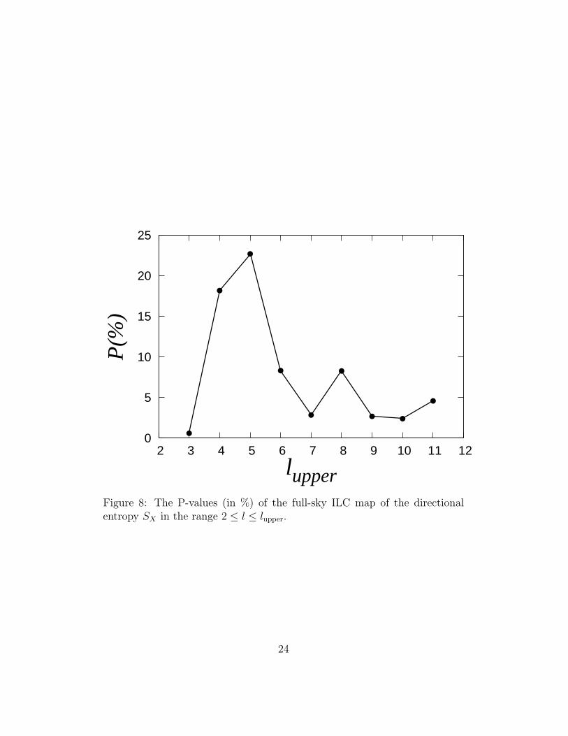
What about the directional entropy ? When SX is evaluated for the range2 ≤ l ≤ 11, random samples show SX equal or lower than the ILC Map only440 times out of 10,000, a P -value of 4.4%. This is another indication ofanisotropy. The P-values for different upper limits lupper are shown in Fig. 8.We see that most of the P-values in this range are smaller than 5 %. Finallythe principal axis of X is

nX(2 ≤ l ≤ 11) = (−0.531, 0.117, 0.839 ).

It is well-aligned with Virgo. The signals from 1 ≤ l ≤ 11 evidently comefrom the same source as the signals from the entire range 2 ≤ l ≤ 50.

3.1.3 The Y Matrix

The Y -matrix gives another method to examine visually the angular corre-lations. Fig. 9 shows contour maps (color online) of the Y (l, l′) correlation.The correlation in ideal uncorrelated data should show a diagonal line upto fluctuations. Features of Fig. 9 confirm the other studies of unusual cor-relations in nominally uncorrelated random data. This study complementsthe study with matrix X, which uses principal axes and does not use theinformation contained in the singular values of ψ.

3.2 Foreground Contaminated Maps

Here we study effects of simulated foreground contamination on the powertensor and entropy statistics.

A contour plot shows the input of the simulation in Fig.10, top panel. Themap is made by adding a random CMB map with a simulated synchrotronforeground map (Giardino et al 2002) generated at 23 GHz frequency andnormalized to 2% of the actual foreground strength. Contamination is dom-inantly in the galactic plane using the procedure of .

Our procedure readily senses the contamination. Fig.10, bottom panel,shows the spatial distribution of largest eigenvectors el for the range of mul-tipole moments 2 ≤ l ≤ 50. The vectors lie dominantly in the galactic plane,providing a clear signal of alignment caused by galactic contamination.

Calculation of the entropy of the largest eigenvectors SX(lmax = 50) =0.995 also shows significant anisotropy. The P value for this to occur in a

23

0

5

10

15

20

25

2 3 4 5 6 7 8 9 10 11 12

P(%

)

lupperFigure 8: The P-values (in %) of the full-sky ILC map of the directionalentropy SX in the range 2 ≤ l ≤ lupper.

24

10 20 30 40 50

10

20

30

40

50

10 20 30 40 50

10

20

30

40

50

- 1

- 0.5

0

0.5

1

l'

l

Figure 9: Contour maps of the correlation Y (l, l′) of traceless tensor powerbetween different angular momentum indices l. Left: a simple density plot.Right: Contours interpolated with trends more readily visible. A scale (coloronline) shows the color code of correlation values. Features confirm the otherstudies of unusual correlations in supposedly uncorrelated random CMBdata.

random isotropic sky is P = 0.01 %. The principal axis, or largest eigenvectorof X is n = (−0.233, −0.963, −0.132), which nicely corresponds to (l =76.4, b = 7.56), lying close to the galactic plane.

These studies show that our procedure detects galactic contamination ina simple and statistically reliable way. They also indicate that the Virgoalignment observed in the preferred directions of the ILC data cannot beattributed to in-plane galactic contamination.

4 Masked Sky Studies

As mentioned in the introduction, our use of linear transformations allowsthe effects of window functions of masks to be handled by conventional andtransparent means. In this Section we explore the effects of masks applied todifferent hemispheres of the galaxy. Although masks distort power spectra,using symmetrical masking creates no biases.

We use four different masks. The Northern and Southern hemispheres ingalactic coordinates are retained in Mask 1 (M1(n)) and Mask 2 (M2(n)),

25

Figure 10: Top panel: Simulated CMB + (2%) synchrotron contaminated fore-ground map described in the text. The simulated foreground contamination is 2%of the actual foreground strength. Bottom panel: Principal axes for 2 ≤ l ≤ 50made from the map of the top panel show alignment in the plane of the galaxy.Mollweide projection in galactic coordinates.

26

respectively. Cone Mask 1 (CM1(n)) and Cone Mask 2 (CM2(n)) respec-tively retain the polar angle regions 0 ≤ θ ≤ 30◦ and 150◦ ≤ θ ≤ 180◦. Theseare typical values chosen to minimize galactic contamination. We show theILC Map cut by M1 and CM1 in Fig. 11.

4.1 Isotropic Maps Estimated from Masked Maps

We explore the power estimated for a full-sky map, as commonly developedfrom the power spectrum obtained from unmasked regions. A window func-tion W (n) is defined so that

∆Tmask(n) = W (n)∆T (n).

This relation is linear and invertible, and already in its diagonal form:

∆T (n) = ∆Tmask(n)/W (n) (18)

Inversion is unstable (“ill-conditioned”) for small W (n), the region whereinformation does not exist, a fact that naturally limits to information thatcan reliably be obtained.

We used the method of Hivon et al, as we briefly review. Let alm(mask)be the amplitude obtained from ∆Tmask(n). The transformation of Eq. 18can be carried out in angular momentum coordinates, with the general form

alm(mask) = W ll′

mm′al′m′ ,

|a(l)(mask)〉 = W ll′ |a(l′)〉 , (19)

where W is the transformed kernel. In general all components of alm(mask),and not just the power spectrum are needed. The power spectrum is relatedby

〈a(l)(mask) | a(l)(mask)〉 = 〈a(l′′)|∑

l

W l′′l∗W ll′ |a(l′)〉 . (20)

An estimate of the power spectrum from inverting Eq. 20 will be linear butgenerally couple all multipoles in complicated ways.

To construct an inversion Hivon et al make the assumption of isotropy.In Eq. 20 replace

〈m | a(l)〉 〈a(l′′) | m′′〉 → Clδll′′δmm′′ . (21)

27

Figure 11: The WMAP-ILC map after applying masks M1(n) and CM1(n).

28

Assuming this applies to ensemble averages, the linear relation between powermeasures is:

< Cl(mask) >=∑

l′

Mll′ < Cl′ >, (22)

where Ml1l2 is computed with Clebsch (3j) coefficients

Ml1l2 =2l2 + 1

4π

l3=l1+l2∑

l3=|l1−l2|

(2l3 + 1)Wl3

(

l1 l2 l30 0 0

)2

(23)

Here Wl is the power spectrum of the mask function. Beam and pixel factorsare readily incorporated in Eq. 22, while for our purposes they can be ab-sorbed into the symbols. Since Eq. 22 is linear, the kernel M can be invertedto solve for estimated Cl of an ideal full sky in terms of the observable powerCl(mask).

In general inversion remains ill-conditioned, and care must be used ininterpretation. Hivon et al choose to work with binned power spectra definedby a running average:

Cb =∑

l

PblCl(mask). (24)

The “binning operator” Pbl we use averages 3 multipoles, with

Cb =

lbmax∑

l=lbmin

l(l + 1)

2πCl(mask)/3

. Binning may ameliorate correlations caused by windowing, while generallycreating its own correlations between different Cb. The estimated full skypower spectrum Cb′ is

Cb′ =∑

b′

K−1b′b Cb;

Kbb′ = (P ·M ·Q)bb′

The ”Inverse binning operator” Qlb is given by Qlb = 2πl(l+1)

and is nonzero

only if 2 ≤ lbmin ≤ l ≤ lbmax. This summarizes sophisticated data processingprocedures applied to the BOOMERANG experiment and many others.

29

We tested our code for full sky power spectrum estimation using Monte-Carlo simulation. We generated 100 random CMB maps, masked them byeach of the four masks, and obtained partial sky power spectra. We binnedthe average masked sky power coefficients to decrease dimensions from anoriginal size of 1024×1024 to a reduced size of 341×341. Finally we producedan estimated full sky power. Figure 12 shows the results of the simulations.The estimated full sky power spectrum matches quite well with the averageof the input full sky binned power spectra for each of the four masks.

We note that the binning and isotropic assumptions of the full sky es-timation method naturally dilute statistical measures. We did not pursuedthe systematic errors. We simply applied our procedures and studied theoutcomes.

4.2 Features of Estimated Full Sky Spectra

In Figure 13 we show the estimated full sky power spectra obtained from ILCusing the four masks M1(n), M2(n) and CM1(n), CM2(n). We observe adefinite asymmetry in the estimated full-sky power spectrum between theNorthern and Southern hemisphere in several multipole ranges.

It is interesting that M1(n), M2(n) and CM1(n), CM2(n) find similarexcess in the same multipole ranges. This shows that the power anisotropyobserved cannot be explained away by contamination of the galactic plane,but also exists at high galactic latitude. To quantify the power differential wesum the difference in power over all bins. The probability of randomly gettingan equal or larger difference is less than 1 % for the range 2 ≤ l ≤ 11 andabout 9 % for the range 2 ≤ l ≤ 50. These figures are given retrospectivelyafter scanning the figures, and one may feel they represent a search. Giventhe unknown systematic errors we will not bother estimating significance. Itis nevertheless interesting that a strictly power-based search, which includesaveraging features that tend to wash out signals, can still potentially detectanisotropy.

Just for interest we also include the estimated full sky ILC power froman unbinned inversion (Fig. 14). There are substantial differences from thebinned evaluation. For example, negative power occurs in some cases. Sincethe unbinned procedure retains more information about the inversion thanbinning, it is a symptom of the instability of inversion, and not a mathemat-ical error. Use of binning helps to cure the problem for an ensemble of manymaps, but it weakens the relation of any particular map to any particular

30

1000

2000

3000

4000

5000

6000

1 10 100

Cll(

l+1)

/(2π

) µ

Κ2

Multipole, l

M1M2

Theory Cl

-200

-100

0

100

10 100D

iff.,

µ Κ

2

Multipole, l

M1 - TheoryM2 - Theory

1000

2000

3000

4000

5000

6000

1 10 100

Cll(

l+1)

/(2π

) µ

Κ2

Multipole, l

CM1CM2

Theory Cl

-200

-100

0

100

200

10 100

Dif

f. µ

Κ2

Multipole, l

CM1- TheoryCM2- Theory

Figure 12: Comparison of estimated full sky power spectrum with input powerspectrum simulation using only masked regions. Blue (red) online denote theNorthern and Southern Hemisphere cases respectively. Top panel: Mask 1 andMask 2. Bottom panel: Cone Mask 1 and Cone Mask 2. The spectra matchthe average of the spectra generating them (solid black line, “Theory”) nearly tothe upper limits of power developed in the maps, l ∼ 300. The inset shows thedifference Diff.

31

200

400

600

800

1000

1200

1400

1600

0 5 10 15 20 25 30 35 40 45 50

l(l+

1)C

l/(2π

) [µ

K2 ]

Multipole,l

M1(n)M2(n)

0

200

400

600

800

1000

1200

1400

1600

1800

2000

0 5 10 15 20 25 30 35 40 45 50

l(l+

1)C

l/(2π

) [µ

K2 ]

Multipole,l

CM1(n)CM2(n)

Figure 13: Estimated full sky binned power spectra, Northern and Southerngalactic hemisphere, using M1(n) and M2(n)(upper panel) and CM1(n) andCM2(n) (lower panel).

32

-1000

-500

0

500

1000

1500

2000

2500

3000

3500

4000

0 5 10 15 20 25 30 35 40 45 50

l(l+

1)C

l/(2π

) [µ

K2 ]

Multipole,l

M1(n)M2(n)

Figure 14: The estimated full sky power map constructed from Mask 1 with-

out going through the running average (“binning”) procedure that combinesdifferent Cl. Note that negative power is sometimes predicted.

data. Exploring such features gives an idea of the reliability of trying toimprove instabilities of inversion by binning.

5 Summary and Conclusions

We have developed several new symmetry-based methods to test CMB datafor isotropy.

The wave function ψkm(l) is a linear transformation of the amplitudes

alm which expresses them as products of vectors and representations l. Thepower tensor Aij is quadratic in the wave functions and alm. Invariants ofthe power tensor are its eigenvalues, the singular values of ψ. The statisticaldistribution of these invariants is a test of randomness and isotropy of thethe power tensor l by l. The power entropy serves as a robust statistic.The power entropy is independent of the usual power, and also independentof the eigenvalues of Aij , which contain information on the orientation ofmultipoles. To assess multipole orientations, we collected the principal axisof Aij , which is the eigenvector with largest eigenvalue.

Both the power entropy and the axial vector distributions show featuresthat are not consistent with isotropy. Fig. 15 summarizes some results of theILC-full sky study. The figure repeats Fig. 1 highlighting the exceptionalcases. Cases of very low power entropy are joined by a short thing line.

33

Λα

l

~

Figure 15: Normalized singular values versus l with exceptional cases highlighted.Thin short lines denote P -values of entropy Spower . 5%. Thick gray lines denoteprincipal axes aligned with the quadrupole (Virgo) axis with P . 5%. There are12 independent cases of 5% or lower significance, which is unlikely in isotropicdata at significance exceeding 99.9%. Significance is increased when the dipole isincluded.

34

Cases of very high alignment of the principal axis with the quadrupole axisare shown by a longer thick gray line. There are 12 independent cases hav-ing 5% probability or lower in an isotropic distribution, with 2 coincidencesshowing both exceptional power entropy and alignment. Ignoring the doublecoincidences, there are 98 independent trials in examining 2 < l < 49 twice.The total probability to see the data’s values in uncorrelated isotropic CMBmaps is of order 10−3.

Our study substantially extends previous studies that find low l multi-poles of current CMB maps are highly unlikely on statistical grounds. Unlikemethods that produce a large number of vector factors for each l, our wavefunction method identifies a single invariant axis for each l, and 3 indepen-dent invariants for each l. The axial quantities are remarkably aligned withthe direction of Virgo in rather systematic fashion for many l. CMB datashow 7 total axes aligned over the range 1 < l < 50, with each case hav-ing independent probability at order 5% or smaller. The values of l= 6, 16,17, 30, 34, 40 have anomalously non-random power eigenvalue distributionsgiving exceptionally lower power entropy. Multipoles with l = 3, 9, 16, 21,40, 43 have anomalous alignment with the quadrupole. It is no longer possi-ble to restrict anomalous CMB statistics to the relative orientation or powerseen in the dipole, quadrupole and octupole cases. Our study shows, forthe first time, that the alignment of the multipoles with an axis pointing inthe direction of Virgo is much more pervasive and not just confined to low lvalues.

To explore the origin of these features, including possible foreground ef-fects, we repeated many calculations using sky-masked data sets. The datashows evidence for systematic differences between the Northern and South-ern regions of the sky. Masking out the galactic plane does not eliminatesignals of anisotropy seen in the full sky studies. As consistency checks,the anisotropies of CMB plus simulated synchrotron emission contaminationfrom the plane of the galaxy are detected by our methods in just the spatialregions where they are simulated. The observed anisotropies cannot readilybe explained away by appealing to galactic foreground contamination.

Acknowledgement We acknowledge the use of Legacy Archive forMicrowave Background Data Analysis. Pramoda acknowledges CSIR, In-dia for finacial support under the research grant CSIR-SRF-9/92(340)/2004-EMR-I. Ralston is supported in part under DOE Grant Number DE-FG02-04ER14308.

35

6 Appendix

Here we relate the factorization wave function ψkm to covariant canonical

forms of the multipoles alm.In the theory of angular momentum one conventionally decomposes prod-

ucts of representations of dimensions j1, j2 into sums of states |JM〉, where|j1 − j2| < J < j1 + j2. It is also possible to divide the large representation|JM〉 into products of smaller representations. Let ΨJ

M = 〈JM | Ψ〉 be thematrix elements of a state |Ψ〉 transforming on representation J . We write

ΨJM → ψj1j2

m1m2= Γj1m1j2m2∗

JM ΨJM , (25)

where the Clebsh-Gordan coefficients are

Γj1m1j2m2∗JM = 〈j1m1j2m2 | JM〉 .

The Clebsch’s dividing angular momentum J in products of j1 = 1 andj2 = J are simply the angular momentum generators ~J cast into the angularmomentum basis. The relation of ψk

m to ψj1j2m1m2

uses |Ψ〉 → |a(l)〉, sets m =m1, converts one Cartesian index k into angular momentum m2, uses j1 = 1and j2 = J = i.

There exist a large number of decompositions for different choices of fac-torization. Each particular choice has a privileged status when viewed as theunique way to factor the multiplet into products of smaller spaces. There isno principle upon which to choose the smaller spaces, explaining the remarkthat no preferred canonical form exists for high-rank tensors. The relationof ψk

m to the canonical form of Copi et al can be viewed as coming from twosteps. First divide |a〉 → (j1 = 1) ⊗ (j1 = 1) ⊗ ..(j2 = 1)... ⊗ .(jl = 1), todevelop the Maxwell multipoles. Next find a unique preferred vector whichmultiplies a tensor of rank l made from traceless symmetric products of theother vectors. That vector corresponds to ψk

m. Alternatively ψkm can sim-

ply be written down (Ralston and Jain 2004) as the vector available fromsymmetry.

References

Abramo, L. R., Sodre Jr., L., Wuensche, C. A., 2006, Phys. Rev. D74,083515

Armendariz-Picon, C., 2004, JCAP 0407, 007

36

Armendariz-Picon, C., 2006, JCAP 0603, 002

Battye, R. A., Moss, A., 2006, Phys. Rev. D74, 04130

Bernui, A., Villela, T., Wuensche, C. A., Leonardi, R., Ferreira, I.,2006, Astron. Astrophys. 454, 409

Bernui, A., Mota, B., Reboucas, M. J., Tavakol, R., 2007, Astron.Astrophys. 464, 479

Bietenholz, M. F., Kronberg, P. P., 1984, ApJ, 287, L1-L2

Bielewicz, P., Gorski, K. M., Banday, A.J., 2004, MNRAS, 355, 1283

Bielewicz, P., Eriksen, H. K., Banday, A. J., Gorski, K. M., Lilje, P.B., 2005, ApJ 635, 750

Birch, P., 1982, Nature, 298, 451

Buniy, R. V., Berera, A., Kephart, T. W., Phys. Rev. D73, 063529

Campanelli, L., Cea, P., Tedesco, L., 2007, arXiv:0706.3802

Cline, J. M., Crotty, P., Lesgourgues, J., 2003, JCAP 0309, 010, astro-ph/0304558;

Contaldi, C. R., Peloso, M, Kofman, L., Linde, A., 2003, JCAP 0307,002, astro-ph/0303636

Copi, C. J., Huterer, D., Schwarz, D. J, Starkman, G. D., 2006, MN-RAS 367, 79

Copi, C. J., Huterer, D., Schwarz, D. J, Starkman, G. D., 2007, Phys.Rev. D75, 023507

da Silva. V., Lim, L-H., 2006, math-0607647

de Oliveira-Costa, A., Tegmark, M., Zaldarriaga, M., Hamilton, A.,2004, Phys. Rev. D 69, 063516, astro-ph/0307282

de Oliveira-Costa, A., Tegmark, M., 2006, Phys. Rev. D74, 023005

Dennis, M. R., 2005, J. Phys. A 38, 1653, arXiv:math-ph/0410004

Donoghue E. P., Donoghue, J. F., 2005, Phys. Rev. D71, 043002

37

Efstathiou, G., 2003, MNRAS 346, L26, astro-ph/0306431

Eriksen, H. K. et al, 2004, ApJ 605, 14

Eriksen, H. K. et al, 2007, ApJ 656, 641

Freeman, P. E., Genovese, C.R., Miller, C.J., Nichol, R.C., Wasserman,L., 2006, ApJ, 638, 1

Gaztanaga, E., Wagg, J., Multamaki, T., Montana, A., Hughes, D. H.,2003, MNRAS 346, 47, astro-ph/0304178

Giardino et al. (2002) A & A , 387, 82

Gordon, C., Hu, W., Huterer, D., Crawford, T. 2005, Phys. Rev. D72,103002

Gumrukcuoglu, A. E., Contaldi, C. R., Peloso, M., 2006, astro-ph/0608405

Gumrukcuoglu, A. E., Contaldi, C. R., Peloso, M., 2007, arXiv:0707.4179

Hajian, A., Souradeep, T., Cornish, N. J., 2004, ApJ 618, L63

Hajian, A., Souradeep, T., 2006, Phys. Rev. D74, 123521

Helling, R. C., Schupp, P., Tesileanu T., 2007, Phys. Rev. D74, 063004

Hunt, P., Sarkar, S., 2004, Phys. Rev. D70, 103518

Hinshaw, G. et al., 2003, Astrophys. J., Suppl. Ser. 148, 63

Hinshaw, G. et al, 2007, ApJ Suppl 170, 288

Hivon, E., et al, 2002, ApJ, 567, 2

Hutsemekers, D., 1998 A & A, 332, 41

Hutsemekers, D., Lamy, H., 2001, A & A, 367, 381

Inoue, K. T., Silk, J., 2006, ApJ 648, 23

Jain, P., Narain, G., Sarala, S., 2004, MNRAS, 347, 394

Jain, P, Ralston, J. P., 1999, Mod. Phys. Lett. A14, 417

38

Jain, P., Sarala, S., 2006, J. Astrophysics and Astronomy, 27, 443

Land, K., Magueijo, J., 2005, Phys. Rev. D72, 101302

Land, K., Magueijo, J., 2006, MNRAS 367, 1714

Land, K., Magueijo, J., 2007, MNRAS 378, 153

Katz, G., Weeks, J., 2004, Phys. Rev. D70, 063527

Kendall, D. G., Young, A. G., 1984, MNRAS, 207, 637

Kesden, M. H., Kamionkowski, M., Cooray, A., 2003, Phys. Rev. Lett.91, 221302, astro-ph/0306597

Kogut, A. et al, 2003, Astrophys. J. Suppl., 148, 161

Koivisto, T., Mota, D. F., 2006, Phys. Rev. D73, 083502

Magueijo, J., Sorkin, R. D., 2007, MNRAS Lett. 377, L39

Moffat, J. W., 2005, JCAP 0510, 012

Naselsky, P. D., Verkhodanov, O. V., Nielsen, M. T. B., 2007, arXiv:0707.1484

Nodland, B., Ralston, J. P. Phys. Rev. Lett. 78, 3043 (1997)

Pereira, S., Pitrou, C., Uzan, J.-P., 2007, arXiv:0707.0736

Phinney, E. S., Webster, R. I., 1983, Nature 301, 735

Prunet, S., Uzan, J.-P., Bernardeau, F., Brunier, T., 2005, Phys. Rev.D71, 083508

Rakic, A., Rasanen, S., Schwarz, D. J., 2006, MNRAS 369, L27

Ralston, J. P., Jain, P., 1999, Int. J. Mod. Phys. D 8, 537.

Ralston, J. P., Jain, P., 2004, Int. J. Mod. Phys., D13, 1857

Rodrigues, D. C., 2007, arXiv:0708.1168

Saha, R., Jain, P. and Souradeep, T., 2006, ApJ Lett., 645, L89

39

Schwarz, D. J., Starkman, G. D., Huterer, D., Copi, C. J., 2004, Phys.Rev. Lett. 93, 221301

Slosar, A., Seljak, U., 2004, Phys. Rev. D70, 083002

Tegmark, M., de Oliveira-Costa, A. and Hamilton, A., 2003, Phys.Rev. D 68, 123523

Vale, C., 2005, astro-ph/0509039

Von Neumann, J., 1932, The Mathematical Foundations of Quantum

Mechanics translated by R. T. Beyer, (Princeton University Press 1996)

Weeks, J. R., 2004, astro-ph/0412231

Wiaux, Y., Vielva, P., Martinez-Gonzalez, E., Vandergheynst, P., 2006,Phys. Rev. Lett. 96, 151303

40