arX

iv:g

r-qc

/960

4032

v2 9

May

199

6

Chaotic scattering around black holes

Juan M. Aguirregabiria

Fisika Teorikoa, Euskal Herriko Unibertsitatea, P. K. 644, 48080 Bilbo, Spain

Abstract

It is shown that the scattering of a charged test particle by a system of

four extreme Reissner-Nordtrom black holes is chaotic in some cases. The

fractal structure of the scattering angle and time delay functions is another

manifestation of the existence of a nonattracting chaotic set: fractal basin

boundaries were previously known.

04.25.-g,04.40.Nr,04.70.Bw,95.10.Fh

Typeset using REVTEX

1

I. INTRODUCTION

The appearance of deterministic chaos in general relativity has been analyzed mainly

in two different contexts: the evolution of cosmological models [1] and the motion of test

particles in prescribed backgrounds. In the last context we may mention the study of charged

particles in interaction with gravitational waves [2] and in the Ernst spacetime [3] and the

chaotic motion of spinless [4] and spinning particles [5] around a Schwarzchild black hole

and a Schwarzchild black hole with quadrupolar and octupolar contributions of arbitrary

strength [6] , but the main interest has been deserved by the system of two extreme Reissner-

Nordstrom black holes described by the Majumdar-Papapetrou (MP) static solutions [7,8].

Chandrasekhar [9] and Contopoulos [10] analyzed the timelike and null geodesics around

these two black holes and described the appearance of chaotic trajectories and their geo-

metric source has been discussed by Yurtsever [11]. Another aspect of chaos, fractal basin

boundaries, have been studied by Dettmann, Frankel and Cornish [12] for the case of two and

three static black holes in the MP geometry and by Drake, Dettmann, Frankel and Cornish

[13] in the context of Special Relativity. These fractal boundaries are consequence of the

existence of a nonattracting chaotic set whose dimension provides a coordinate independent

measure of chaos [14].

The goal of this paper is to show that, for a different range of parameters, another conse-

quence of the existence of a nonattracting chaotic set arises in multi-black-hole spacetimes:

chaotic scattering [15]. We will consider a static system of four extreme Reissner-Nordstrom

black holes and a test particle, with e/m > 1. For certain energy ranges, the scattering is

chaotic both in the relativistic system and in the Newtonian approximation. To the best of

our knowledge this is the first time that chaotic scattering angle and time delay functions

are described in general relativity [16].

2

II. THE EQUATIONS OF MOTION

Majumdar [7] and Papapetrou [8] independently showed that the metric

ds2 = −U−2 dt2 + U2(

dx2 + dy2 + dz2)

(1)

is a static solution of the Einstein-Maxwell equations corresponding to the electrostatic

potential A = U−1 dt if the function U(x, y, z) satisfies Laplace’s equation:

U,xx + U,yy + U,zz = 0. (2)

Hartle and Hawking [17] showed that if one chooses

U = 1 +N

∑

i=1

mi

|x − xi|, (3)

the MP solution represents N extremal (qi = mi) Reissner-Nordstrom black holes held

at the fixed positions, x = xi, under the combined action of gravitational attraction and

electrostatic repulsion. The apparent singularity of U at the points xi corresponds to the

usual coordinate singularity at an event horizon.

Let us now consider a test particle of mass m and charge e moving in the above multi-

black-hole geometry. Following Dettmann, Frankel and Cornish [12] we can write its equa-

tions of motion in the form

x = U−1v, (4)

v = U−2

[(

1 + 2v · v − e

mγ

)

∇U − (v · ∇U)v

]

, (5)

t = Uγ, (6)

γ ≡√

1 + v · v, (7)

where a dot indicates the derivative with respect to the proper time and (γ,v) are the

components of the four-velocity in an orthonormal frame. The conserved energy per unit

mass is

E = U−1

(

γ − e

m

)

. (8)

3

III. CHAOTIC SCATTERING

Contopoulos [10] analyzed the case of an uncharged particle (e/m = 0) moving around

N = 2 static black holes and discussed the role of periodic orbits and the route to chaos

through a cascade of period-doubling bifurcations. Dettmann, Frankel and Cornish [12]

considered the cases N = 2, 3 for a particle with e/m ≤ 1 which was released from rest.

Under these circumstances the gravitational attraction overcomes the electrostatic repulsion

and the particle will fall into one of the black holes or orbit indefinitely, but will not es-

cape to infinity. Dettmann, Frankel and Cornish showed that the boundary separating in

phase-space the different asymptotic behaviors is fractal, which indicates the presence of a

nonattracting chaotic set [15] whose dimension provides a coordinate independent measure

of chaos [14].

We have considered the motion of a charged test particle in the plane (x, y) around a

system of four equal Reissner-Nordtrom black holes which are at rest at points (±1,±1, 0)

and have qi = mi = 1/3. The energy (8) has not exactly the same structure as in Newtonian

mechanics, but we can still get the same kind of qualitative information given by the turning

points of the potential if we study the curves of zero velocity [10], i.e., curves in the (x, y)

plane which satisfy Eq. (8) for v = 0. Orbits never cross the curves of zero velocity.

If e/m > 1 the electrostatic repulsion acting on a stationary test particle is stronger than

the gravitational attraction and for (1 + 2√

2/3)−1(1− e/m) < E < 0 there exist a curve of

zero velocity around each black hole. In Fig. 1 we have the right hand side of (8) for v = 0

and e/m = 2. The curves of zero velocity are the contours of constant height of the displayed

surface. In these circumstances, we will have scattering: orbits coming from infinity will

escape to infinity, they will not fall into one of the black holes. But there exist another set

(of measure zero but non-null dimension) of orbits which are not trapped by a single black

hole: the unstable periodic orbits in which the particle bounces forever between different

repulsion centers or, more precisely, between different curves of zero velocity. This is the

kind of scenario in which chaotic scattering is likely to appear [15]. Although this system

4

does not fit exactly in one of the classes in which chaotic scattering is usually analyzed, i.e.,

gradient systems and hard disks or spheres, we expect to have a similar qualitative behavior

because we still have curves of zero velocity (which are the curves in which the energy equals

the potential energy in the case of gradient systems and the perimeter of hard disks).

In the following, we consider a test particle with e/m = 2 which is sent from the point

(−4, b, 0), for different values of the impact parameter b, and with initial velocity (v, 0, 0).

The v value is selected in order to have always an energy per unit mass E = −0.45. As

can be seen in Fig. 2, for this value of the energy per unit mass there exist a curve of zero

velocity around each black hole preventing orbits coming from infinity to be trapped by the

black holes.

The system (4)-(5) is numerically solved by means of an ordinary-differential-equation

solver [18]. The quality of the numerical results is tested by using different integration

schemes, ranging from the very stable embedded Runge-Kutta code of eight order due to

Dormand and Prince to very fast extrapolation routines. All codes have adaptive step size

control and we check that smaller tolerances do not change the results. Furthermore, the

constancy of the energy (8) is monitored to test the integration accuracy.

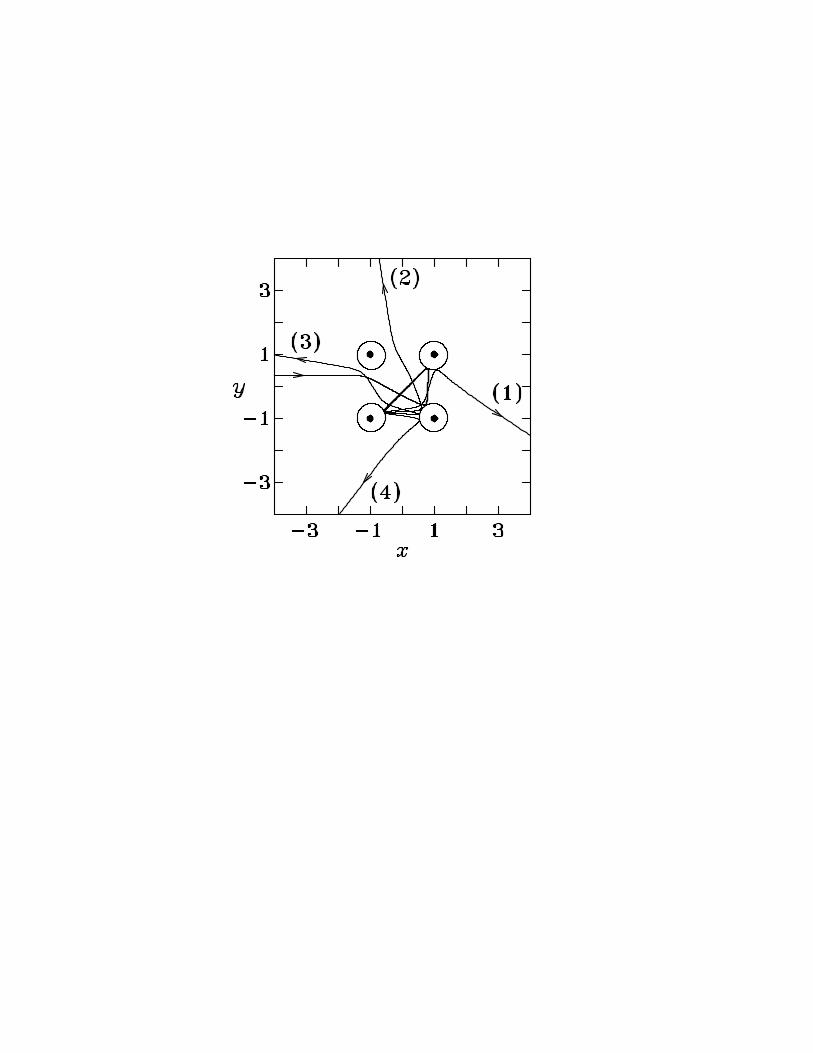
In Fig. 2 we see four orbits which correspond to very close initial conditions, but look

very different after bouncing several times on different curves of zero velocity. This sensitive

dependence on initial conditions is the hallmark of chaos. To explore this further we have

chosen a large number of points (∼ 2 × 105) in the interval 0.34 ≤ b ≤ 0.42 and integrated

the system for each initial condition until the particle escapes the system. (In practice we

consider that the particle has abandoned the system when |x| > 10, because it cannot return

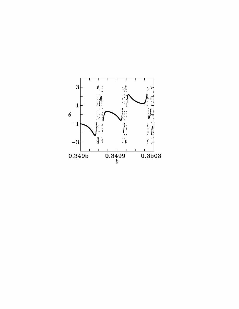
if E < 0.) Then we compute the scattering angle θ between the velocity v and the x axis. In

Fig. 3 we have plot 2000 points of the scattering function θ(b). In some ranges the function

is continuous and the points are located on a smooth curve, but in other intervals the points

are wildly scattered because θ(b) is discontinuous at the points of a Cantor set, as can be

seen in the blowups of Figs. 4 and 5 where smaller and smaller subintervals are analyzed.

The (approximate) scale invariance typical of fractals is apparent. This kind of phenomenon

5

is called “chaotic scattering” [15].

IV. TIME DELAYS AND THE UNCERTAINTY DIMENSION

Exactly as in ordinary Hamiltonian systems [15], the singularity points of the scatter-

ing function correspond to unstable periodic orbits in which the particles bounces forever

between the curves of zero velocities of different black holes. This can be seen in Fig. 6

where the time the particle spends in the scattering region is plotted against the impact

parameter b. This time goes to infinity precisely at the singularity points of θ(b). It is

easy to understand that if two orbits are initially very close but then come near one of the

unstable periodic orbits, they will spend a very long time inside the scattering region and

the accumulated defocusing effect of the successive bounces will yield rather different exit

angles.

Though the fractal nature of the scattering function is apparent from the approximate

autosimilarity shown in Figs. 3, 4 and 5, we can make this fact more quantitative by using

a variation of the “uncertainty exponent technique” [15], which is also used in determining

the dimension of fractal basin boundaries. We select a uncertainty value ǫ and sample the

interval under study by choosing points in the form bi+1 = bi + ǫ. If for the three values

bi−1, bi and bi+1 the particle scatters upward or the three values correspond to a downward

scattering, we say that the bi value is ǫ-certain. The remaining bi points are the ǫ-uncertain

values and correspond to cases in which an error of magnitude ǫ in the determination of

the initial conditions will prevent us from predicting if the particle will finally escape the

scattering region upward or downward. A measure of the uncertainty is thus given by the

fraction of ǫ-uncertain values which we will call f(ǫ).

It has been found in many different contexts that this magnitude scale with respect to ǫ

according to a power law:

f(ǫ) ∼ ǫα, (9)

where α is the “uncertainty exponent.” When the set of uncertain points (in the limit

6

ǫ → 0) is not fractal it is easy to see that α = 1 − D, where D is the ordinary dimension of

the set. This relation is extended to fractal cases by defining the “uncertainty dimension”

as D ≡ 1 − α and it has been conjectured that this definition will coincide with the “box

counting” dimension [15]. The meaning of the uncertainty dimension is that if we divide by

10 the error in the determination of the impact parameter, we only reduce by an amount of

101−D the error in the prediction of the late-time behavior. High values of D (0 <= D < 1 in

our case) make very difficult improving our predictions. This is the obstacle to predictability

in chaotic scattering.

In Fig. 7, some values of the fraction of ǫ-uncertain values f(ǫ) in the interval 0.34 ≤ b ≤

0.42 are plotted on a log-log scale. One sees that the points are fitted very well by a straight

line of slope α = 0.49. We conclude that the power law (9) is satisfied and the uncertainty

dimension of the singularity set of the system under study is

D = 1 − α = 0.51. (10)

This dimension provides a coordinate independent measure of chaos [14].

V. FINAL COMMENTS

We have shown that a charged test particle may experience the phenomenon of chaotic

scattering around a static system formed by four extreme Reissner-Nordstrom black holes: in

some cases the scattering angle (and time delay) function is singular at the points of a Cantor

set. As mentioned above, another manifestation of the existence of a nonattracting chaotic

set, fractal basin boundaries, was previously known for MP solutions, but for other values

of the parameters. In some sense this kind of chaotic behavior is less surprising, because it

does not appear for N = 1, 2 (which are the only cases with an integrable Newtonian limit

[12]). For N > 2, we have repeated the analysis made above for the Newtonian limit, and

it is not difficult to find parameter ranges for which the scattering becomes chaotic. Let us

also mention that the same happens in the relativistic case. For instance, we have found

7

that chaotic scattering also happens around three black holes, though we have chosen to

present here the more symmetric case N = 4.

ACKNOWLEDGMENTS

I would like to thank N. J. Cornish for useful criticisms and for pointing out some relevant

references. This work has been supported by The University of the Basque Country under

contract UPV/EHU 172.310-EB036/95.

8

REFERENCES

[1] See, for instance, D. Hobill, A. Burd and A. Coley (eds.), Deterministic Chaos in General

Relativity, (Plenum Press, New York, 1994).

[2] H. Varvoglis and D. Papadopoulos, Astron. Astrophys. 261, 664 (1992).

[3] V. Karas and D. Vokrouhlicky, Gen. Relativ. Gravit. 24, 729 (1992).

[4] L. Bombelli and E. Calzetta, Class. Quantum Grav. 9 2573 (1992).

[5] S. Suzuki and K. Maeda, preprint gr-qc/9604020.

[6] W. M. Vieira and P. S. Letelier, Phys. Rev. Lett. 76, 1409 (1996).

[7] S. D. Majumdar, Phys. Rev. 72, 390 (1947);

[8] A. Papapetrou, Proc. R. Irish Acad. A51, 191 (1947).

[9] S. Chandrasekhar, Proc. Roy. Soc. London A421, 227 (1989).

[10] G. Contopoulos, Proc. Roy. Soc. London A431, 183 (1990); A435, 551 (1991)

[11] U. Yurtsever, Phys. Rev. D 52, 3176 (1995).

[12] C. P. Dettmann, N. E. Frankel and N. J. Cornish, Phys. Rev. D 50, R618 1994; Fractals

3, 161 (1995).

[13] S. P. Drake, C. P. Dettmann, N. E. Frankel and N. J. Cornish, Phys. Rev. E 53, 1351

1996.

[14] N. J. Cornish, preprint gr-qc/9602054.

[15] E. Ott, Chaos in Dynamical Systems, (Cambridge University Press, New York, 1993).

[16] N. J. Cornish and J. Levin have also computed scattering angles and time delays for

two and three black holes (unpublished). N. J. Cornish, private communication.

[17] J. B. Hartle and S. W. Hawking, Commun. Math. Phys. 26, 87 (1972).

9

[18] J. M. Aguirregabiria, ODE Workbench, (American Institute of Physics, New York,

1994).

10

FIGURES

FIG. 1. Energy per unit mass (8) for v = 0 and e/m = 2.

FIG. 2. Four black holes at points (±1,±1, 0) have curves of zero velocity around them for

E = −0.45 and e/m = 2. Orbits corresponding to (1) b = 0.34975, (2) b = 0.34971875, (3)

b = 0.3496875 and (4) b = 0.34965625 are also depicted.

FIG. 3. The scattering function θ(b) for 0.34 ≤ b ≤ 0.42.

FIG. 4. A blowup of Fig. (3) showing the scattering function θ(b) for 0.36 ≤ b ≤ 0.44.

FIG. 5. A further blowup of Figs. (3) and (4).

FIG. 6. The time-delay function indicating the time the particle spends in the scattering region

for each value of the impact parameter. It becomes infinite at the singularity points of Fig. (3).

FIG. 7. A log-log plot of the fraction of uncertain values f(ǫ) for different resolutions ǫ. The

straight line fit has a slope α = 0.49.

11

-2

-1

0

1

2 -2

-1

0

1

2

-0.4

-0.2

0

-2

-1

0

1

2