arX

iv:1

004.

1327

v2 [

cond

-mat

.mes

-hal

l] 2

0 M

ay 2

011

The Density of States of Chaotic Andreev Billiards

Jack Kuipers,1, ∗ Thomas Engl,1, † Gregory Berkolaiko,2 Cyril Petitjean,1, 3 Daniel Waltner,1 and Klaus Richter1

1Institut fur Theoretische Physik, Universitat Regensburg, D-93040 Regensburg, Germany2Department of Mathematics, Texas A&M University, College Station, TX 77843-3368, USA

3SPSMS, UMR-E 9001, CEA-INAC/UJF-Grenoble 1,17 Rue des Martyrs, 38054 Grenoble Cedex 9, France

(Dated: May 23, 2011)

Quantum cavities or dots have markedly different properties depending on whether their classicalcounterparts are chaotic or not. Connecting a superconductor to such a cavity leads to notableproximity effects, particularly the appearance, predicted by random matrix theory, of a hard gap inthe excitation spectrum of quantum chaotic systems. Andreev billiards are interesting examples ofsuch structures built with superconductors connected to a ballistic normal metal billiard since eachtime an electron hits the superconducting part it is retroreflected as a hole (and vice-versa). Usinga semiclassical framework for systems with chaotic dynamics, we show how this reflection, alongwith the interference due to subtle correlations between the classical paths of electrons and holesinside the system, is ultimately responsible for the gap formation. The treatment can be extendedto include the effects of a symmetry breaking magnetic field in the normal part of the billiard or anAndreev billiard connected to two phase shifted superconductors. Therefore we are able to see howthese effects can remold and eventually suppress the gap. Furthermore, the semiclassical frameworkis able to cover the effect of a finite Ehrenfest time, which also causes the gap to shrink. Howeverfor intermediate values this leads to the appearance of a second hard gap - a clear signature of theEhrenfest time.

PACS numbers: 74.40.-n,03.65.Sq,05.45.Mt,74.45.+c

I. INTRODUCTION

The physics of normal metals (N) in contact with su-perconductors (S) has been studied extensively for al-most fifty years, and in the past two decades there hasbeen somewhat of a resurgence of interest in this field.This has mainly been sparked by the realization of ex-periments that can directly probe the region close to thenormal-superconducting (NS) interface at temperaturesfar below the transition temperature of the superconduc-tor. Such experiments have been possible thanks to mi-crolithographic techniques that permit the building ofheterostructures on a mesoscopic scale combined withtransport measurements in the sub-Kelvin regime. Suchhybrid structures exhibit various new phenomena, mainlydue to the fact that physical properties of both the super-conductor and the mesoscopic normal metal are stronglyinfluenced by quantum coherence effects.

The simplest physical picture of this system is that thesuperconductor tends to export some of its anomalousproperties across the interface over a temperature depen-dent length scale that can be of the order of a micrometerat low temperatures. This is the so-called proximity ef-fect, which has been the focus on numerous surveys; bothexperimental1–9 and theoretical10–13.

The key concept to understand this effect14–16 is An-dreev reflection. During this process, when an electronfrom the vicinity of the Fermi energy (EF) surface of thenormal conductor hits the superconductor, the bulk en-ergy gap ∆ of the superconductor prevents the negativecharge from entering, unless a Cooper pair is formed inthe superconductor. Since a Cooper pair is composed

of two electrons, an extra electron has to be taken fromthe Fermi sea, thus creating a hole in the conductionband of the normal metal. Physically and classicallyspeaking, an Andreev reflection therefore corresponds toa retroflection of the particle, where Andreev reflectedelectrons (or holes) retrace their trajectories as holes (orelectrons). The effect of Andreev reflection on the trans-port properties of open NS structures is an interestingand fruitful area (see Refs. 17,18 and references thereinfor example), though in this paper we focus instead onclosed structures. Naturally this choice has the conse-quence of leaving aside some exciting recent results suchas, for example, the statistical properties of the conduc-tance19, the magneto-conductance in Andreev quantumdots20, resonant tunneling21 and the thermoelectrical ef-fect22,23 in Andreev interferometers.

In closed systems, one of the most noticeable mani-festations of the proximity effect is the suppression ofthe density of states (DoS) of the normal metal justabove the Fermi energy. Although most of the exper-imental investigations have been carried out on disor-dered systems1,3,5,6,8, with recent technical advances in-terest has moved to structures with clean ballistic dynam-ics2,4,7,9,24,25. This shift gives access to the experimentalinvestigation of the so-called Andreev billiard. While thisterm was originally coined26 for an impurity-free normalconducting region entirely confined by a superconductingboundary, it also refers to a ballistic normal area (i.e. aquantum dot) with a boundary that is only partly con-nected to a superconductor. The considerable theoreticalattention raised by such a hybrid structure in the pastdecade is related to the interesting peculiarity that bylooking at the DoS of an Andreev billiard we can deter-

2

mine the nature of the underlying dynamics of its classi-cal counterpart27. Indeed, while the DoS vanishes witha power law in energy for the integrable case, the spec-trum of a chaotic billiard is expected to exhibit a true gapabove EF

27. The width of this hard gap, also called theminigap13, has been calculated as a purely quantum ef-fect by using random matrix theory (RMT) and its valuescales with the Thouless energy, ET = ~/2τd, where τd isthe average (classical) dwell time a particle stays in thebilliard between successive Andreev reflections27.

Since the existence of this gap is expected to be relatedto the chaotic nature of the electronic motion, many at-tempts have been undertaken to explain this result insemiclassical terms28–34, however this appeared to berather complicated. Indeed a traditional semiclassicaltreatment based on the so-called Bohr-Sommerfeld (BS)approximation yields only an exponential suppression ofthe DoS28–30. This apparent contradiction of this pre-diction with the RMT one was resolved quite early byLodder and Nazarov28 who pointed out the existenceof two different regimes. The characteristic time scalethat governs the crossover between the two regimes isthe Ehrenfest time τE ∼ | ln ~|, which is the time scalethat separates the evolution of wave packets following es-sentially the classical dynamics from longer time scalesdominated by wave interference. In particular it is theratio τ = τE/τd, that has to be considered.

In the universal regime, τ = 0, chaos sets in sufficientlyrapidly and RMT is valid leading to the appearance ofthe aforementioned Thouless gap27. Although the Thou-less energy ET is related to a purely classical quantity,namely the average dwell time, we stress that the appear-ance of the minigap is a quantum mechanical effect, andconsequently the gap closes if a symmetry breaking mag-netic field is applied35. Similarly if two superconductorsare attached to the Andreev billiard, the size of the gapwill depend on the relative phase between the two super-conductors, with the gap vanishing for a π-junction35.

The deep classical limit is characterized by τ → ∞, andin this regime the suppression of the DoS is exponentialand well described by the BS approximation. The moreinteresting crossover regime of finite Ehrenfest time, andthe conjectured Ehrenfest time gap dependence of Ref. 28have been investigated by various means12,21,36–40. Dueto the logarithmic nature of τE, investigating numeri-cally the limit of large Ehrenfest time is rather difficult,but a clear signature of the gap’s Ehrenfest time depen-dence has been obtained41–43 for τ < 1. From an an-alytical point of view RMT is inapplicable in the finiteτE regime12, therefore new methods such as a stochasticmethod38 using smooth disorder and sophisticated per-turbation methods that include diffraction effects36 havebeen used to tackle this problem. On the other hand apurely phenomenological model, effective RMT, has beendeveloped37,44 and predicts a gap size scaling with theEhrenfest energy EE = ~/2τE. Recently Micklitz andAltland40, based on a refinement of the quasiclassical ap-proach and the Eilenberger equation, succeeded to show

the existence of a gap of width πEE ∝ 1/τ in the limitof large τ≫1.Consequently a complete picture of all the available

regimes was still missing until recently when we treatedthe DoS semiclassically45 following the scattering ap-proach46. Starting for τ = 0 and going beyond the diago-nal approximation we used an energy-dependent general-ization of the work47 on the moments of the transmissioneigenvalues. The calculation is based on the evaluationof correlation functions also appearing in the momentsof the Wigner delay times48. More importantly, the ef-fect of finite Ehrenfest time could be incorporated in thisframework49 leading to a microscopic confirmation of theτE dependence of the gap predicted by effective RMT.Interestingly the transition between τ = 0 and τ = ∞is not smooth and a second gap at πEE was observedfor intermediate τ , providing us with certainly the mostclear-cut signature of Ehrenfest time effects.In this paper we extend and detail the results obtained

in45. First we discuss Andreev billiards and their treat-ment using RMT and semiclassical techniques. For theDoS in the universal regime (τ = 0) we first delve intothe work of Refs. 47,48 before using it to obtain the gen-erating function of the correlation functions which areemployed to derive the DoS. This is done both in theabsence and in the presence of a time reversal symme-try breaking magnetic field, and we also look at the casewhen the bulk superconducting gap and the excitationenergy of the particle are comparable.We then treat Andreev billiards connected to two su-

perconducting contacts with a phase difference φ. Thegap is shown to shrink with increasing phase differencedue to the the accumulation of a phase along the trajec-tories that connect the two superconductors. Finally theEhrenfest regime will be discussed, especially the appear-ance of a second intermediate gap for a certain range ofτ . We will also show that this intermediate gap is verysensitive to the phase difference between the supercon-ductors.

II. ANDREEV BILLIARDS

Since the treatment of Andreev billiards was recentlyreviewed in Ref. 13 we just recall some useful details here.In particular the chaotic Andreev billiard that we con-sider is treated within the scattering approach46 wherethe NS interface is modelled with the help of a ficti-tious ideal lead. This lead permits the contact betweenthe normal metal cavity (with chaotic classical dynam-ics) and the semi-infinite superconductor as depicted inFig. 1a.Using the continuity of the superconducting and nor-

mal wave function, we can construct the scattering ma-trix of the whole system. Denoting the excitation energyof the electron above the Fermi energy EF by E and as-suming that the lead supports N channels (transversemodes at the Fermi energy), the scattering matrix of the

3

(a)

S N

(b)

S N

e

h

FIG. 1: (a) The Andreev billiard consists of a chaotic normalmetal (N) cavity attached to a superconductor (S) via a lead.(b) At the NS interface between the normal metal and thesuperconductor electrons are retroreflected as holes.

whole normal region can be written in a joint electron-hole basis and reads

SN(E) =

(

S(E) 00 S∗(−E)

)

, (1)

where S(E) is the unitary N × N scattering matrix ofthe electrons (and its complex conjugate S∗(−E) thatof the holes). As the electrons and holes remain un-coupled in the normal region the off-diagonal blocks arezero. Instead, electrons and holes couple at the NS in-terface through Andreev reflection15 where electrons areretroreflected as holes and vice versa, as in Fig. 1b. Forenergies E smaller than the bulk superconductor gap ∆there is no propagation into the superconductor and if weadditionally assume ∆ ≪ EF we can encode the Andreevreflection in the matrix

SA(E) = α(E)

(

0 11 0

)

, (2)

α(E) = e−i arccos(E∆ ) =

E

∆− i

√

1− E2

∆2. (3)

The retroreflection (of electrons as holes with thesame channel index) is accompanied by the phase shiftarccos (E/∆). In the limit of perfect Andreev reflection(E = 0) this phase shift reduces to π/2.Below ∆ the Andreev billiard has a discrete excitation

spectrum at energies where det [1− SA(E)SN(E)] = 0,which can be simplified46 to

det[

1− α2(E)S(E)S∗(−E)]

= 0. (4)

Finding the roots of this equation yields the typical den-sity of states of chaotic Andreev billiards. In the next twoSections we review the two main analytical frameworksthat can be used to tackle this problem.

A. Random matrix theory

One powerful treatment uses random matrix theory.Such an approach was initially considered in Refs. 27,35

(a)

S1

+φ2

N1

N S2

−φ2

N2

⊗

B

(b)

S1

S2

FIG. 2: (a) An Andreev billiard connected to two supercon-ductors (S1, S2) at phases ±φ/2 via leads carrying N1 and N2

channels, all threaded by a perpendicular magnetic field B.(b) The semiclassical treatment involves classical trajectoriesretroreflected at the superconductors an arbitrary number oftimes.

where the actual setup treated is depicted in Fig. 2a.It consists of a normal metal (N) connected to two su-perconductors (S1, S2) by narrow leads carrying N1 andN2 channels. The superconductors’ order parameters areconsidered to have phases±φ/2, with a total phase differ-ence φ. Moreover a perpendicular magnetic field B wasapplied to the normal part. We note that although thisfigure (and Fig. 1a) have spatial symmetry the treatmentis actually for the case without such symmetry.As above, the limit ∆ ≪ EF was taken so that normal

reflection at the NS interface can be neglected and thesymmetric case in which both leads contain the samenumber, N/2, of channels was considered27,35. Finally itwas also assumed that α ≈ −i, valid in the limit E,ET ≪∆ ≪ EF. For such a setup, the determinantal equation(4) becomes

det[

1 + S(E)eiφS∗(−E)e−iφ]

= 0, (5)

where φ is a diagonal matrix whose first N/2 elementsare φ/2 and the remaining N/2 elements −φ/2. We notethat though we stick to the case of perfect coupling here,the effect of tunnel barriers was also included in Ref. 27.The first step is to rewrite the scattering problem in

terms of a low energy effective Hamiltonian H

H =

(

H πXXT

−πXXT −H∗

)

, (6)

where H is theM×M Hamiltonian of the isolated billiardand X an M ×N coupling matrix. Eventually the limitM → ∞ is taken and to mimic a chaotic system thematrix H is replaced by a random matrix following thePandey-Mehta distribution17

P (H) ∝ exp

(

−N2(

1 + a2)

64ME2T

(7)

×M∑

i,j=1

[

(

ReHij

)2

+ a−2(

ImHij

)2]

.

4

The parameter a measures the strength of the time-reversal symmetry breaking so we can investigate thecrossover from the ensemble with time-reversal symme-try, the Gaussian orthogonal ensemble (GOE), to thatwithout, the Gaussian unitary ensemble (GUE). It is re-lated to the magnetic flux Φ through the two-dimensionalbilliard of area A and with Fermi velocity vF by

Ma2 = c

(

eΦ

h

)2

~vFN

2πET

√A. (8)

Here c is a numerical constant of order unity dependingonly on the shape of the billiard. The critical flux is thendefined via

Ma2 =N

8

(

Φ

Φc

)2

⇔ Φc ≈h

e

(

2πET

~vF

)12

A14 .

(9)The density of states, divided for convenience by twice

the mean density of states of the isolated billiard, can bewritten as

d(ǫ) = −ImW (ǫ), (10)

where W (ǫ) is the trace of a block of the Green functionof the effective Hamiltonian of the scattering system andfor simplicity here we express the energy in units of theThouless energy ǫ = E/ET. This is averaged by inte-grating over (7) using diagrammatic methods50, whichto leading order in inverse channel number 1/N leads tothe expression35

W (ǫ) =

(

b

2W (ǫ)− ǫ

2

)

(

1 +W 2(ǫ) +

√

1 +W 2(ǫ)

β

)

,

(11)

where β = cos (φ/2) and b = (Φ/Φc)2with the critical

magnetic flux Φc for which the gap in the density of statescloses (at φ = 0). Equation (11) may also be rewrittenas a sixth order polynomial and when substituting into(10), we should take the solution that tends to 1 for largeenergies. In particular, when there is no phase differencebetween the two leads (φ = 0, or equivalently when weconsider a single lead carrying N channels) and no mag-netic field in the cavity (Φ/Φc = 0) the density of statesis given by a solution of the cubic equation

ǫ2W 3(ǫ) + 4ǫW 2(ǫ) + (4 + ǫ2)W (ǫ) + 4ǫ = 0. (12)

B. Semiclassical approach

The second approach, and that which we pursue anddetail in this paper, is to use the semiclassical approxima-tion to the scattering matrix which involves the classicaltrajectories that enter and leave the cavity51. Using thegeneral expression between the density of states and thescattering matrix52, the density of states of an Andreevbilliard reads30,46,53

d(E) = d− 1

πIm

∂

∂Eln det [1− SA(E)SN(E)] , (13)

where d = N/2πET is twice the mean density of statesof the isolated billiard (around the Fermi energy). Equa-tion (13) should be understood as an averaged quantityover a small range of the Fermi energy or slight variationsof the billiard and for convergence reasons a small imag-inary part is included in the energy E. In the limit ofperfect Andreev reflection α(E) ≈ −i, see (3), and (13)reduces to

d(E) = d+1

πIm

∂

∂ETr

∞∑

m=1

1

m

(

0 iS∗(−E)iS(E) 0

)m

.

(14)Obviously only even terms in the sum have a non-zerotrace, and setting n = 2m, dividing through by d andexpressing the energy in units of the Thouless energyǫ = E/ET, this simplifies to30

d(ǫ) = 1 + 2Im

∞∑

n=1

(−1)n

n

∂C(ǫ, n)

∂ǫ. (15)

Equation (15) involves the correlation functions of n scat-tering matrices

C(ǫ, n) =1

NTr

[

S∗(

− ǫ~

2τd

)

S

(

ǫ~

2τd

)]n

, (16)

where we recall that the energy is measured relative tothe Fermi energy and that ET = ~/2τd involves the aver-age dwell time τd. For chaotic systems54 the dwell timecan be expressed as τd = TH/N in terms of the Heisen-berg time TH conjugate to the mean level spacing (2/d).At this point it is important to observe that nonzero

values of ǫ are necessary for the convergence of the ex-pansion of the logarithm in (13) that led to (15). On theother hand, we are particularly interested in small valuesof ǫ which puts (15) on the edge of the radius of con-vergence, where it is highly oscillatory. The oscillatorybehavior and a slow decay in n is a direct consequenceof the unitarity of the scattering matrix at ǫ = 0 (in fact

later it can also be shown that ∂C(ǫ,n)∂ǫ |ǫ=0 = in). Thus a

truncation of (15) will differ markedly from the predictedRMT gap, which was the root of the difficulty of captur-ing the gap by previous semiclassical treatments30,33,34.In the present work we succeed in evaluating the entiresum and hence obtain results which are uniformly validfor all values of ǫ.Calculating the density of states is then reduced to

the seemingly more complicated task of evaluating cor-relation functions semiclassically for all n. Luckily thetreatment of such functions has advanced rapidly in thelast few years47,48,55–57 and we build on that solid basis.We also note that determining C(ǫ, n) is a more gen-eral task than calculating the density of states. Sincethe Andreev reflection has already been encoded in theformalism before (15), the treatment of the C(ǫ, n) nolonger depends on the presence or absence of the super-conducting material, but solely on the properties of thechaotic dynamics inside the normal metal billiard.

5

(a) (b) (c) (d)

FIG. 3: (a) The original trajectory structure of the correlation function C(ǫ, 2) where the incoming channels are drawn on theleft, outgoing channels on the right, electrons as solid (blue) and holes as dashed (green) lines. (b) By collapsing the electrontrajectories directly onto the hole trajectories we create a structure where the trajectories only differ in a small region called anencounter. Placed inside the Andreev billiard this diagram corresponds to Fig. 2b. The encounter can be slid into the incomingchannels on the left (c) or the outgoing channels on the right (d) to create diagonal-type pairs.

In the semiclassical approximation, the elements of thescattering matrix are given by51

Soi(E) ≈ 1√TH

∑

ζ(i→o)

AζeiSζ(E)/~, (17)

where the sum runs over all classical trajectories ζ start-ing in channel i and ending in channel o. Sζ(E) is theclassical action of the trajectory ζ at energy E above theFermi energy and the amplitude Aζ contains the stabilityof the trajectory as well as the Maslov phases58. After wesubstitute (17) into (16) and expand the action aroundthe Fermi energy up to first order in ǫ using ∂Sζ/∂E = Tζ

where Tζ is the duration of the trajectory ζ, the correla-tion functions are given semiclassically by a sum over 2ntrajectories

C(ǫ, n) ≈ 1

NT nH

n∏

j=1

∑

ij ,oj

∑

ζj(ij→oj)

ζ′

j(oj→ij+1)

AζjA∗ζ′

jei(Sζj

−Sζ′j)/~

×eiǫ(Tζj

+Tζ′j)/(2τd)

. (18)

The final trace in (16) means that we identify in+1 = i1and as the electron trajectories ζj start at channel ij andend in channel oj while the primed hole trajectories ζ′j gobackwards starting in channel oj and ending in channelij+1 the trajectories fulfill a complete cycle, as in Figs. 3aand 4a,d,g. The channels i1, . . . , in will be referred to asincoming channels, while o1, . . . , on will be called outgo-ing channels. This refers to the direction of the electrontrajectories at the channels and not necessarily to whichlead the channel finds itself in (when we have two leadsas in Fig. 2).

The actions in (18) are taken at the Fermi energy andthe resulting phase is given by the difference of the sumof the actions of the unprimed trajectories and the sum ofthe actions of the primed ones. In the semiclassical limitof ~ → 0 (c.f. the RMT limit of M → ∞) this phaseoscillates widely leading to cancellations when the aver-aging is applied, unless this total action difference is ofthe order of ~. The semiclassical treatment then involvesfinding sets of classical trajectories that can have such asmall action difference and hence contribute consistentlyin the limit ~ → 0.

III. SEMICLASSICAL DIAGRAMS

As an example we show the original trajectory struc-ture for n = 2 in Fig. 3a, where for convenience we drawthe incoming channels on the left and the outgoing chan-nels on the right so that electrons travel to the right andholes to the left (c.f. the shot noise in Refs. 59–61). Ofcourse the channels are really in the lead (Fig. 1a) or ei-ther lead (Fig. 2) and the trajectory stretches involvemany bounces at the normal boundary of the cavity.We draw such topological sketches as the semiclassicalmethods were first developed for transport47,55,57 wheretypically we have S† (complex conjugate transpose) in-stead of S∗ (complex conjugate) in (16), restricted to thetransmission subblocks, so that all the trajectories wouldtravel to the right in our sketches. Without the mag-netic field, the billiard has time reversal symmetry andS is symmetric, but this difference plays a role when weturn the magnetic field on later. An even more impor-tant difference is that in our problem any channel can bein any lead.

To obtain a small action difference, and a possible con-tribution in the semiclassical limit, the trajectories mustbe almost identical. This can be achieved for exampleby collapsing the electron trajectories directly onto thehole trajectories as in Fig. 3b. Inside the open circle,the holes still ‘cross’ while the electrons ‘avoid cross-ing’, but by bringing the electron trajectories arbitrarilyclose together the set of trajectories can have an arbi-trary small action difference. More accurately, the exis-tence of partner trajectories follows from the hyperbol-icity of the phase space dynamics. Namely, given twoelectron trajectories that come close (have an encounter)in the phase space, one uses the local stable and unsta-ble manifolds62–64 to find the coordinates through whichhole trajectories arrive along one electron trajectory andleave along the other, exactly as in Fig. 3b (and Fig. 2b).These are the partner trajectories we pick for ζ′1 and ζ′2when we evaluate C(ǫ, 2) from (18) in the semiclassicalapproximation. As the encounter involves two electrontrajectories it is called a 2-encounter. An encounter canhappen anywhere along the length of a trajectory. Inparticular, it can happen at the very beginning or thevery end of a trajectory, in which case it is actually hap-pening next to the lead, see Figs. 3c,d. This situationis important as it will give an additional contribution to

6

(a) (b) (c)

(d)

i1

i2

i3

i4

o1

o2

o3

o4(e)

i1

i4

i2

i3

o1

o4

o2

o3(f)

i1

i4

i2

i3

o1

o4

o2

o3

(g)

i1

i4

i2

i3

o1

o4

o2

o3

(h)

i1

o1

i2

o2

i3

o3

i4

o4

(i)

i1

o1 i2

o2

i3

o3

i4 o4

FIG. 4: (a) The original trajectory structure of the correlation function C(ǫ, 4) where the incoming channels are drawn on theleft, outgoing channels on the right, electrons as solid (blue) and holes as dashed (green) lines. (d,g) Equivalent 2D projectionsof the starting structure as the order is determined by moving along the closed cycle of electron and hole trajectories. (b)By pinching together the electron trajectories (pairwise here) we can create a structure which only differs in three smallregions (encounters) and which can have a small action difference. (e) Projection of (b) also created by collapsing the electrontrajectories in (g) directly onto the hole trajectories. (c,f) Sliding two of the encounters from (b) together (or originally pinching3 electron trajectories together) creates these diagrams. (h,i) Resulting rooted plane tree diagrams of (e,f) or (b,c) defining thetop left as the first incoming channel (i.e. the channel ordering as depicted in (e,f)).

that of an encounter happening in the body of the bil-liard. We will refer to this situation as an ‘encounterentering the lead’. We note that if an encounter entersthe lead the corresponding channels must coincide and wehave diagonal-type pairs (i.e. the trajectories are coupledexactly pairwise) though it is worth bearing in mind thatthere is still a partial encounter happening near the leadas shown by the Ehrenfest time treatment60,65.

To give a more representative example, consider thestructure of trajectories for n = 4. For visualization pur-poses in Fig. 4a the original trajectories are arrangedaround a cylinder in the form of a cat’s cradle. The in-coming and outgoing channels are ordered around thecircles at either end although they could physically beanywhere. Projecting the structure into 2D we can drawit in several equivalent ways, for example as in Fig. 4dor 4g, and we must take care not to overcount such equiv-alent representations. We note that the ordering of thechannels is uniquely defined by the closed cycle that thetrajectories form. To create a small action difference,we can imagine pinching together the electron (and hole)strings in Fig. 4a. One possibility is to pinch two together

in three places (making three 2-encounters) as in Fig. 4b.A possible representation in 2D is shown in Fig. 4e, whichcan also be created by collapsing the electron trajectoriesdirectly onto the hole trajectories in Fig. 4g. Note thatthe collapse of the diagram in Fig. 4d leads to a differentstructure with three 2-encounters. However in general itis not true that the different projections of the arrange-ment in Fig. 4a are in a one-to-one correspondence withall possible diagrams.

From Figs. 4b,e we can create another possibility bysliding two of the 2-encounters together to make a 3-encounter (or alternatively we could start by pinchingthree trajectories together in Fig. 4a as well as an ad-ditional pair) as in Fig. 4c,f. Finally we could combineboth to a single 4-encounter. Along with the possibilitieswhere all the encounters are inside the system, we canprogressively slide encounters into the leads, as we didfor the n = 2 case in Fig. 3, creating, among others, thediagrams in Fig. 5.

Finally, we mention that so far we were listing only‘minimal’ diagrams. One can add more encounters tothe above diagrams but we will see later that such ar-

7

(a) (b) (c)

(d) (e) (f)

FIG. 5: Further possibilities arise from moving encounters into the lead(s). Starting from Fig. 4c we can slide the 2-encounterinto the outgoing channels on the right (called ‘o-touching’, see text) to arrive at (a,d) or the 3-encounter into the incomingchannels on the left (called ‘i-touching’) to obtain (b,e). Moving both encounters leads to (c,f), but moving both to the sameside means first combining the 3- and 2-encounter in Fig. 4c into a 4-encounter and is treated as such.

rangements contribute at a higher order in the inversenumber of channels and are therefore subdominant. Thecomplete expansion in this small parameter is availableonly for small values of n, see Refs. 56,57,59.

A. Tree recursions

To summarize the previous paragraph, the key tasknow is to generate all possible minimal encounter ar-rangements (see, for example, Ref. 48 for the completelist of those with n = 3). This is a question that was an-swered in Ref. 47 where the moments of the transmissionamplitudes were considered. The pivotal step was to re-draw the diagrams as rooted plane trees and to show thatthere is a one-to-one relation between them (for the dia-grams that contribute at leading order in inverse channelnumber). To redraw a diagram as a tree we start with aparticular incoming channel i1 as the root (hence rootedtrees) and place the remaining channels in order aroundan anticlockwise loop (hence plane). Moving along thetrajectory ζ1 we draw each stretch as a link and each en-counter as a node (open circle) until we reach o1. Thenwe move along ζ′1 back to its first encounter and continuealong any new encounters to i2 and so on. For example,the tree corresponding to Figs. 4b,e is drawn in Fig. 4hand that corresponding to Figs. 4c,f is in Fig. 4i. Notethat marking the root only serves to eliminate overcount-ing and the final results do not depend on the particularchoice of the root.A particularly important property of the trees is their

amenability to recursive counting. The recursions be-hind our treatment of Andreev billiards were derived inRef. 47 and we recall the main details here. First we candescribe the encounters in a particular tree by a vectorv whose elements vl count the number of l-encounters in

the tree (or diagram); this is often written as 2v23v3 · · · .An l-encounter is a vertex in the tree of degree 2l (i.e.connected to 2l links). The vertices of the tree that corre-spond to encounters will be called ‘nodes’, to distinguishthem from the vertices of degree 1 which correspond tothe incoming and outgoing channels and which will becalled ‘leaves’. The total number of nodes is V =

∑

l>1 vland the number of leaves is 2n where n is the order ofthe correlation function C(ǫ, n) to which the trees con-tribute. Defining L =

∑

l>1 lvl, we can express n asn = (L − V + 1). Note that the total number of links isL+n which can be seen as l links trailing each l-encounterplus another n from the incoming channels. For example,the 2131 tree in Fig. 4i has L = 5, V = 2 and contributesto the n = 4 correlation function. We always draw thetree with the leaves ordered i1, o1, . . . , in, on in anticlock-wise direction. This fixes the layout of the tree in theplane, thus the name ‘rooted plane trees’66.

From the start tree, we can also move some encountersinto the lead(s) and it is easy to read off when this is pos-sible. If an l-encounter (node of degree 2l) is adjacent toexactly l leaves with label i it may ‘i-touch’ the lead, i.e.the electron trajectories have an encounter upon enter-ing the system and the corresponding incoming channelscoincide. Likewise if a 2l-node is adjacent to l o-leaves itmay ‘o-touch’ the lead. For example, in Fig. 4i the topnode has degree 6, is adjacent to 3 i-leaves (including theroot) and can i-touch the lead as in Figs. 5b,e. The lowerencounter can o-touch as in Figs. 5a,d. In addition, bothencounters can touch the lead to create Figs. 5c,f.

Semiclassically, we add the contributions of all the pos-sible trajectory structures (or trees) and the contributionof each is made up by multiplying the contributions of itsconstituent parts (links, encounters and leaves). First wecount the orders of the number of channels N . As men-tioned in Ref. 47 (see also Sec. IV below) the multiplica-

8

o1

i2o2 i3 o3

i4o4

i5

o5 i6 i7o8

i8 o8

i9o9

(a)i1

o6

(b)i1

o1

i2

o2

(c)o2

i3 o3

i4o4

i5

o5 i6

(d)i6

o6

(e)o6

i7o8

i8

(f)i8

o8

i9

o9

FIG. 6: The tree shown in (a) is cut at its top node (of degree 6) such that the trees (b)-(f) are created. Note that to completethe five new trees we need to add an additional four new links and leaves and that the trees (c) and (e) in the even positionshave the incoming and outgoing channels reversed.

tive contribution of each encounter or leaf is of order Nand each link gives a contribution of order 1/N . Togetherwith the overall factor of 1/N , see equation (16), the to-tal power of 1/N is γ, the cyclicity of the diagram. Sinceour diagrams must be connected, the smallest cyclicity isγ = 0 if the diagram is a tree. The trees can be gener-ated recursively, since by cutting a tree at the top nodeof degree 2l (after the root) we obtain 2l− 1 subtrees, asillustrated in Fig. 6.To track the trees and their nodes, the generating func-

tion F (x, zi, zo) was introduced47 where the powers of

• xl enumerate the number of l-encounters,

• zi,l enumerate the number of l-encounters that i-touch the lead,

• zo,l enumerate the number of l-encounters that o-touch the lead.

Later we will assign values to these variables which willproduce the correct semiclassical contributions of thetrees. Note that the contributions of the links and leaveswill be absorbed into the contributions of the nodes hencewe do not directly enumerate the links in the generatingfunction F . Inside F we want to add all the possibletrees and for each have a multiplicative contribution ofits nodes. For example, the tree in Fig. 4i and its relativesin Fig. 5 would contribute

x3x2 + zi,3x2 + x3zo,2 + zi,3zo,2 = (x3 + zi,3) (x2 + zo,2) .(19)

A technical difficulty is that the top node may (if thereare no further nodes) be able to both i-touch and o-touch,but clearly not at the same time. An auxiliary generat-ing function f = f(x, zi, zo) is thus introduced with the

restriction that the top node is not allowed to i-touchthe lead. We denote by ‘empty’ a tree which contains noencounter nodes (like Fig. 6d). An empty tree is assignedthe value 1 (i.e. f(0) = 1) to not affect the multiplica-tive factors. To obtain a recursion for f we separate thetree into its top node of degree 2l and 2l − 1 subtreesas in Fig. 6. As can be seen from the Figure, l of thenew trees (in the odd positions from left to right) startwith an incoming channel, while the remaining l−1 evennumbered subtrees start with an outgoing channel, andcorrespond to a tree with the i’s and o’s are reversed. For

these we use the generating function f where the roles ofthe z variables corresponding to leaves of one type are

switched so f = f(x, zo, zi). The tree then has the con-tribution of the top node times that of all the subtrees

giving xlflf l−1.

The top node may also o-touch the lead, but for thisto happen all the odd-numbered subtrees must be empty(i.e. they must contain no further nodes and end directlyin an outgoing channel). When this happens we justget the contribution of zo,l times that of the l − 1 even

subtrees: zo,lfl−1. In total we have

f = 1 +

∞∑

l=2

[

xlflf l−1 + zo,lf

l−1]

, (20)

and similarly

f = 1 +

∞∑

l=2

[

xlflf l−1 + zi,lf

l−1]

. (21)

For F we then reallow the top node to i-touch the leadwhich means that the even subtrees must be empty and

9

a contribution of zi,lfl, giving

F = f +

∞∑

l=2

zi,lfl =

∞∑

l=1

zi,lfl, (22)

if we let zi,1 = 1 (and also zo,1 = 1 for symmetry). Pick-ing an o-leaf as the root instead of an i-leaf should leadto the same trees and contributions so F should be sym-

metric upon swapping zi with zo and f with f . Theserecursions enumerate all possible trees (which representall diagrams at leading order in inverse channel number)and we now turn to evaluating their contributions to thecorrelation functions C(ǫ, n).

IV. DENSITY OF STATES WITH A SINGLE

LEAD

To calculate the contribution of each diagram,Refs. 55–57 used the ergodicity of the classical motionto estimate how often the electron trajectories are likelyto approach each other and have encounters. Combinedwith the sum rule55,67 to deal with the stability ampli-tudes, Ref. 56 showed that the semiclassical contributioncan be written as a product of integrals over the dura-tions of the links and the stable and unstable separationsof the stretches in each encounter. One ingredient is thesurvival probability that the electron trajectories remaininside the system (these are followed by the holes whoseconditional survival probability is then 1) which classi-cally decays exponentially with their length and the de-cay rate 1/τd = N/TH. A small but important effect isthat the small size of the encounters means the trajec-tories are close enough to remain inside the system orescape (hit the lead) together so only one traversal ofeach encounter needs to be counted in the total survivalprobability

exp

(

− N

THtx

)

, tx =

L+n∑

i=1

ti +

V∑

α=1

tα, (23)

where the ti are the durations of the (n+L) link stretchesand tα the durations of the V encounters so that theexposure time tx is shorter than the total trajectory time(which includes l copies of each l-encounter).As reviewed in Ref. 57 the integrals over the links and

the encounters (with their action differences) lead to sim-ple diagrammatic rules whereby

• each link provides a factor of TH/ [N (1− iǫ)] ,

• each l-encounter inside the cavity provides a factorof −N (1− ilǫ) /T l

H ,

with the (1− ilǫ) deriving from the difference betweenthe exposure time and the total trajectory time. Recall-ing the prefactor in (18) and that L is the total numberof links in the encounters, it is clear that all the Heisen-berg times cancel. The channel number factorN−2n from

these rules and the prefactor (with n = L−V +1) cancelswith the sum over the channels in (18) as each of the 2nchannels can be chosen from the N possible channels (toleading order).

With this simplification, each link gives (1− iǫ)−1

,each encounter − (1− ilǫ) and each leaf a factor of 1. Toabsorb the link contributions into those of the encounters(nodes) we recall that the number of links is n+

∑Vα=1 lα,

where α labels the V different encounters. Therefore thetotal contribution factorizes as

1

(1− iǫ)n

V∏

α=1

− (1− ilαǫ)

(1− iǫ)lα

. (24)

Moving an l-encounter into the lead, as in Fig. 5 meanslosing that encounter, l links and combining l channelsso we just remove that encounter from the product above(or give it a factor 1 instead).

A. Generating function

Putting these diagrammatic rules into the recursionsin Sec. III A then simply means setting

xl =− (1− ilǫ)

(1− iǫ)l

· rl−1, zi,l = zo,l = 1 · rl−1, (25)

where we additionally include powers of r to track theorder of the trees and later generate the semiclassicalcorrelation functions. The total power of r of any tree is∑

l>1(l− 1)vl = L−V = n− 1. To get the required pref-

actor of (1− iǫ)−n in (24) we can then make the changeof variable

f = g(1− iǫ), r =r

1− iǫ, (26)

so that the recursion relation (20) becomes

g(1−iǫ) = 1−∞∑

l=2

rl−1glgl−1(1−ilǫ)+

∞∑

l=2

rl−1gl−1, (27)

and similarly for g. Using geometric sums (the first twoterms are the l = 1 terms of the sums) this is

g

1− rgg=

iǫg

(1− rgg)2 +

1

1− rg. (28)

We note that the since f is obtained from f by swappingzi and zo and in our substitution (25) zi = zo, the func-

tions f and f are equal. Taking the numerator of theequation above and substituting g = g leads to

g − 1

1− iǫ=

rg2

1− iǫ[g − 1− iǫ] . (29)

To obtain the desired generating function of the semi-classical correlation functions we set F = G (1− iǫ) in

10

(22), along with the other substitutions in (25) and (26),

G(ǫ, r) =g

1− rg, G(ǫ, r) =

∞∑

n=1

rn−1C(ǫ, n), (30)

so that by expanding g and hence G in powers of r weobtain all the correlation functions C(ǫ, n). This can besimplified by rearranging (30) and substituting into (29)to get the cubic for G directly

r(r−1)2G3+r(3r+iǫ−3)G2+(3r+iǫ−1)G+1 = 0. (31)

B. Density of states

The density of states of a chaotic Andreev billiard withone superconducting lead (15) can be rewritten as

d(ǫ) = 1− 2Im∂

∂ǫ

∞∑

n=1

(−1)n−1C(ǫ, n)

n, (32)

where without the 1/n the sum would just be G(ǫ,−1) inview of (30). To obtain the 1/n we can formally integrateto obtain a new generating function H(ǫ, r),

H(ǫ, r) =1

ir

∂

∂ǫ

∫

G(ǫ, r)dr,

H(ǫ, r) =

∞∑

n=1

rn−1

in

∂C(ǫ, n)

∂ǫ, (33)

so the density of states is given simply by

d(ǫ) = 1− 2ReH(ǫ,−1). (34)

To evaluate the sum in (32) we now need to integratethe solutions of (31) with respect to r and differentiatewith respect to ǫ. Since G is an algebraic generatingfunction, i.e. the solution of an algebraic equation, thederivative of G with respect to ǫ is also an algebraic gen-erating function68. However, this is not generally true forintegration, which can be seen from a simple example off = 1/x, which is a root of an algebraic equation, unlikethe integral of f . Solving equation (31) explicitly andintegrating the result is also technically challenging, dueto the complicated structure of the solutions of the cubicequations. Even if it were possible, this approach wouldfail in the presence of magnetic field, when G is a solutionof a quintic equation, see Sec. IVD, or in the presence ofa phase difference between two superconductors.The approach we took is to conjecture that H(ǫ, r)

is given by an algebraic equation, perform a computer-aided search over equations with polynomial coefficientsand then prove the answer by differentiating appropri-ately. We found that

(ǫr)2(1− r)H3 + iǫr[r(iǫ − 2) + 2(1− iǫ)]H2

+ [r(1 − 2iǫ)− (1− iǫ)2]H + 1 = 0, (35)

when expanded in powers of r, agrees for a range of valuesof n with the expansion of (33) derived from the corre-lation functions obtained from (31). To show that (35)agrees with (33) to all orders in r we use a differentia-tion algorithm to find an equation for the intermediategenerating function

I(ǫ, r) =1

i

∂G(ǫ, r)

∂ǫ=

∂[rH(ǫ, r)]

∂r,

I(ǫ, r) =

∞∑

n=1

rn−1

i

∂C(ǫ, n)

∂ǫ, (36)

both starting from (31) and from (35) and verifying thatthe two answers agree.The differentiation algorithm starts with the algebraic

equation for a formal power series η in the variable xwhich satisfies an equation of the form

Φ(x, η) := p0(x) + p1(x)η + . . .+ pm(x)ηm = 0, (37)

where p0(x), . . . , pm(x) are some polynomials, not all ofthem zero. The aim is to find an equation satisfied byξ = dη/dx, of the form

q0(x) + q1(x)ξ + . . .+ qm(x)ξm = 0, (38)

where q0(x), . . . , qm(x) are polynomials. Differentiating(37) implicitly yields

ξ = −∂Φ(x, η)

∂x

(

∂Φ(x, η)

∂η

)−1

=P (η, x)

Q(η, x), (39)

where P and Q are again polynomial. After substitut-ing this expression into the algebraic equation for ξ andbringing everything to the common denominator we get

q0(x)Qm(x, η) + q1(x)P (x, η)Qm−1(x, η)

+ . . .+ qm(x)Pm(x, η) = 0. (40)

However, this equation should only be satisfied mod-ulo the polynomial Φ(x, η). Namely, we use poly-nomial division and substitute P j(x, η)Qm−j(x, η) =T (x, η)Φ(x, η) +Rj(x, η) into (40). Using (37) we arriveat

q0(x)R0(x, η) + q1(x)R1(x, η) + . . .+ qm(x)Rm(x, η) = 0.(41)

The polynomials Rj are of degree of m− 1 in η. Treat-ing (41) as an identity with respect to η we thus obtainm linear equations on the coefficients qj . Solving thosewe obtain qj as rational functions of x and multiplyingthem by their common denominator gives the algebraicequation for ξ.Performing this algorithm on G from (31), with x = iǫ,

and on rH from (35), with x = r, leads to the sameequation, given as (A.1) in the appendix, for the inter-mediate function defined in (36) and therefore proves thevalidity of the equation (35). Setting ǫ = 0 in (35) then

shows that ∂C(ǫ,n)∂ǫ |ǫ=0 = in as mentioned in Sec. II B.

11

(a) (b)

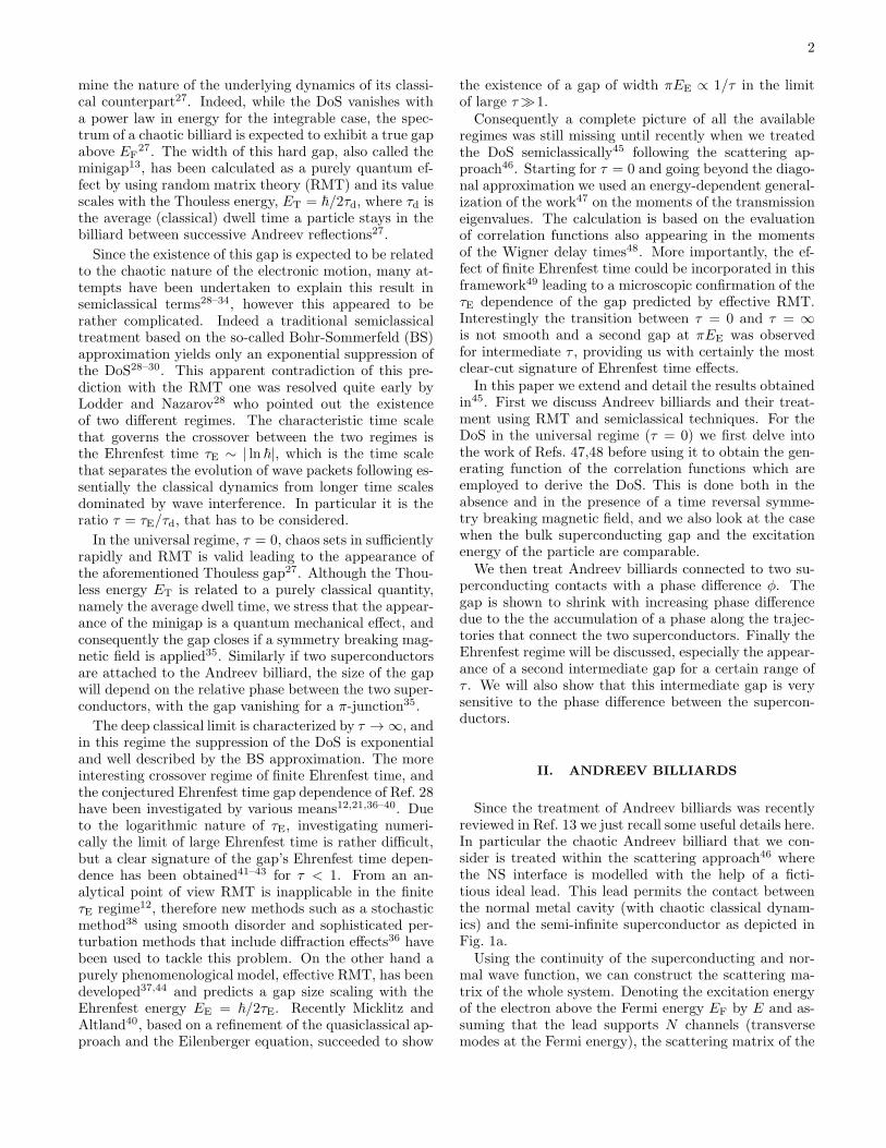
FIG. 7: (a) The density of states of a chaotic quantum dot coupled to a single superconductor at E ≪ ∆. (b) The density ofstates with a finite bulk superconducting gap ∆ = 2ET (dashed line) and ∆ = 8ET (solid line) compared to the previous casein (a) with ∆ → ∞ (dotted line).

To compare the final result (34) with the RMT predic-tion we can substitute H(ǫ,−1) = [−iW (ǫ) + 1] /2 into(35). The density of states is then given in terms of W asd(ǫ) = −ImW (ǫ). The equation for W simplifies to theRMT result (12), and the density of states then reads27

d(ǫ) =

0 ǫ ≤ 2(√

5−12

)5/2

√3

6ǫ [Q+(ǫ)−Q−(ǫ)] ǫ > 2(√

5−12

)5/2 ,

(42)

where Q±(ǫ) =(

8− 36ǫ2 ± 3ǫ√3ǫ4 + 132ǫ2 − 48

)1/3.

This result is plotted in Fig. 7a and shows the hard gapextending up to around 0.6ET.

C. Small bulk superconducting gap

The calculation of the density of states above used theapproximation that the energy was well below the bulksuperconductor gap, E ≪ ∆ or ǫ ≪ δ (for δ = ∆/ET),so that the phase shift at each Andreev reflection wasarccos(ǫ/δ) ≈ π/2. For higher energies or smaller super-conducting gaps, however, the density of states should bemodified69 to

d(ǫ) = 1 + Re2√

δ2 − ǫ2+ 2Im

∞∑

n=1

∂

∂ǫ

[

α(ǫ)2nC(ǫ, n)

n

]

,

(43)

where α(ǫ) = δ/(ǫ + i√δ2 − ǫ2) as in (3). When taking

the energy derivative in the sum in (43) we can split theresult into two sums and hence two contributions to thedensity of states

d(ǫ) = 1 + 2Im

∞∑

n=1

α(ǫ)2n

n

∂C(ǫ, n)

∂ǫ(44)

+ Re2√

δ2 − ǫ2

[

1 + 2

∞∑

n=1

α(ǫ)2nC(ǫ, n)

n

]

.

Here the first term, which comes from applying the en-ergy derivative to C(ǫ, n), gives an analogous contribu-tion to the case E ≪ ∆ but with r = α2 instead of −1and involving H(ǫ, α2) from (33) and (35). The secondterm in (44) comes from the energy derivative of α2n andcan be written using G(ǫ, α2) from (30) and (31):

d(ǫ) = Re[

1 + 2α2H(ǫ, α2)]

+Re2√

δ2 − ǫ2

[

1 + 2α2G(ǫ, α2)]

. (45)

The effect of a finite bulk superconducting gap on thehard gap in the density of states of the Andreev billiardis fairly small, for example as shown in Fig. 7b even forδ = ∆/ET = 2 the width just shrinks to around 0.5ET.For δ = 2 the shape of the density of states is changedsomewhat (less so for δ = 8) and we can see just beforeǫ = 2 it vanishes again giving a second thin gap. Thisgap, and even the way we can separate the density ofstates into the two terms in (45), foreshadows the effectsof the Ehrenfest time (in Sec. VI). For energies abovethe bulk superconducting gap (ǫ > δ) we see a thin sin-

gular peak from the√δ2 − ǫ2 which quickly tends to the

density of states of an Andreev billiard with an infinitesuperconducting gap as the energy becomes larger.

D. Magnetic field

If a magnetic field is present, the time reversal symme-try is broken and we wish to treat this transition semi-classically as in Refs. 64,70. Note that since for the lead-ing order diagrams each stretch is traversed in oppositedirections by an electron and a hole we are effectivelyconsidering the same situation as for parametric correla-tions71,72. Either way, the idea behind the treatment isthat the classically small magnetic field affects the classi-cal trajectories very little, but adds many essentially ran-dom small perturbations to the action. The sum of these

12

FIG. 8: The effect of a time reversal symmetry breaking mag-netic field on the density of states of a chaotic Andreev bil-liard with a single superconducting lead for b = 0 (dottedline), b = 1/4 (solid line), b = 1 (dashed line) and b = 9/4(dashed dotted line).

fluctuations is approximated using the central limit the-orem, and leads to an exponential damping so the linksnow provide a factor of TH/N(1− iǫ+ b). The parameter

b is related to the magnetic field via b = (Φ/Φc)2 as in

Sec. II A. For an l-encounter however, as the stretchesare correlated and affected by the magnetic field in thesame way, the variance of the random fluctuations of allthe stretches is l2 that of a single stretch. Hence each en-counter now contributes N

(

1− ilǫ+ l2b)

/T lH and again

the correlation inside the encounters leads to a small butimportant effect.Similarly to the treatment without the magnetic field

above, we can put these contributions into the recursionsin Sec. III A by setting

xl =−(

1− ilǫ+ l2b)

(1− iǫ+ b)l

· rl−1, zi,l = zo,l = 1 · rl−1,

(46)and

f = g(1− iǫ+ b), r =r

1− iǫ+ b. (47)

The intermediate generating function is then given by theimplicit equation

−r2g5 + (1 + iǫ + b)r2g4 + (2− iǫ− b)rg3

− (2 + iǫ− b)rg2 − (1− iǫ + b)g + 1 = 0, (48)

and the generating function G(ǫ, b, r) of the magneticfield dependent correlation functions C(ǫ, b, n), which isstill connected to g via G = g/(1− rg), is given by

r2(r − 1)3G5

+(

iǫr − iǫ + 5r2 − 10r + 5− br − b)

r2G4

+(

3iǫr − iǫ+ 10r2 − 12r + 2− 3br − b)

rG3

+ (3iǫ+ 10r − 6− 3b)rG2

− (1 − 5r − iǫ + b)G+ 1 = 0. (49)

Removing the magnetic field by setting b = 0 reducesboth of these equations (after factorizing) to the pre-vious results (29) and (31). Next we again searchfor and verify an algebraic equation for H(ǫ, b, r) =1/(ir)

∫

[∂G(ǫ, b, r)/∂ǫ]dr, though the higher order makesthis slightly more complicated, finding

4b2r4 (r − 1)H5 + 4br3 [iǫ− 3b+ r (2b− iǫ)]H4

+ r2[

ǫ2 (1− r) + 2iǫb (5− 3r)− b (13b+ 4)

+ br (5b+ 4)]

H3

+ r[

2 (iǫ− 3b) (1− iǫ+ b) (50)

+ r(

(1− iǫ+ b)2+ 4b− 1

)]

H2

−[

(1− iǫ+ b)2 − r (1− 2iǫ+ 2b)

]

H + 1 = 0.

In order to check the agreement with the RMT resultwe substitute H(ǫ, b,−1) = [−iW (ǫ, b) + 1] /2 into (50).This leads to

b2W 5 − 2bǫW 4 −(

4b− b2 − ǫ2)

W 3 + 2(2− b)ǫW 2

+(

4− 4b+ ǫ2)

W + 4ǫ = 0, (51)

which corresponds to the RMT result (11) with no phase(φ = 0). The density of states calculated from this equa-tion is shown in Fig. 8 for different values of b. The gapreduces for increasing b, closes exactly at the critical flux(b = 1) and the density of states becomes flat (at 1) asb → ∞.

V. DENSITY OF STATES WITH TWO LEADS

Next we consider a classically chaotic quantum dotconnected to two superconductors with N1 and N2 chan-nels respectively and a phase difference φ, as depictedin Fig. 2a. The density of states, as in Sec. II A andRefs. 35,69, can then be reduced to equation (15) butwith

C(ǫ, φ, n) =1

NTr

[

S∗(

− ǫ~

2τd

)

e−iφS

(

+ǫ~

2τd

)

eiφ]n

,

(52)

where φ is again a diagonal matrix whose first N1 ele-ments from the first superconductor S1 are φ/2 and theremaining N2 elements from S2 are −φ/2. Note that thecase φ = 0 corresponds to the previous case of a singlesuperconductor with N = N1 + N2 channels. When wesubstitute the semiclassical approximation for the scat-tering matrix (17) into (52), and especially if we write thescattering matrix in terms of its reflection and transmis-sion subblocks, the effect of the superconductors’ phasedifference becomes simple. Namely, each electron (un-primed) trajectory which starts in lead 1 and ends inlead 2 picks up the phase factor exp(−iφ) while each un-primed trajectory going from lead 2 to lead 1 receives thefactor exp(iφ). Reflection trajectories which start and

13

ζ1

ζ2

1ζ’

4ζ’

ζ32ζ’

3ζ’

ζ4

e e+i

1S ,

φ

+ φ2

− φ2

−iφ

S2,

FIG. 9: The paths may start and end in either of the two leadsas shown. ζ4 as it travels from lead 1 to lead 2 obtains a phasefactor exp(−iφ), ζ2 traveling back contributes exp(iφ) whilethe others does not contribute any phase. The encountersare again marked by circles and S1 and S2 denote the twosuperconducting leads at the corresponding superconductingphases ±φ/2. This diagram is equivalent to the one in Fig. 4f.

end in the same lead have no additional phase factor, asdepicted in Fig. 9. Since exchanging the leads gives theopposite phase, we expect the solution to be symmetricif we simultaneously exchange N1 with N2 and change φto −φ.As these factors are multiplicative, we can equivalently

say that each electron trajectory leaving superconductor1 or 2 picks up exp(−iφ/2) or exp(iφ/2) while each oneentering lead 1 or 2 picks up exp(iφ/2) or exp(−iφ/2).To include these factors in our semiclassical diagrams,we can simply remember that in our tree recursions inSec. III A the channels we designated as ‘incoming’ chan-nels have electrons leaving them while electrons alwaysenter the outgoing channels. Each incoming channel (inthe original channel sum in (18)) can still come from theN possible channels, but with the trajectory leaving itnow provides the factor N1 exp(−iφ/2) + N2 exp(iφ/2).Similarly each outgoing channel now provides the com-plex conjugate of this factor. Recalling the power ofN−2n coming from the links and encounters, we can up-date the contribution of each diagram or tree (24) to

(

N1e− iφ

2 +N2eiφ2

)n (

N1eiφ2 +N2e

− iφ2

)n

N2n (1− iǫ)n

×V∏

α=1

− (1− ilαǫ)

(1− iǫ)lα

. (53)

However, moving an l-encounter into lead 1 means com-bining l incoming channels, l links and the encounteritself. These combined incoming channels, with l elec-tron trajectories leaving, will now only give the factorN1 exp(−ilφ/2)+N2 exp(ilφ/2) where the important dif-ference is that l is inside the exponents. We thereforemake the replacement

(

N1e− iφ

2 +N2eiφ2

)l

N l→

(

N1e− ilφ

2 +N2eilφ2

)

N(54)

as well as removing the encounter from (53). Similarly

when we move the encounter into the outgoing leads wetake the complex conjugate of (54).To mimic these effects in the semiclassical recursions

we can set

xl =− (1− ilǫ)

(1− iǫ)l· rl−1,

β =

(

N1e− iφ

2 +N2eiφ2

)

N, (55)

zi,l =

(

N1e− ilφ

2 +N2eilφ2

)

Nβl· rl−1,

zo,l =

(

N1eilφ2 +N2e

− ilφ2

)

N (β∗)l

· rl−1, (56)

f = g(1− iǫ)

ββ∗ , r = rββ∗

(1− iǫ), (57)

in Sec. III A. Including these substitutions in the recur-sion relation (20) and summing we obtain

g

ββ∗ − rgg=

iǫββ∗g

(ββ∗ − rgg)2 +

N1

N

1

β∗e−iφ2 − rg

+N2

N

1

β∗eiφ2 − rg

, (58)

and a similar equation from (21). The generating func-tion of the correlation functions C(ǫ, φ, n) is then givenfrom (22) by

G =N1

N

g

βeiφ2 − rg

+N2

N

g

βe−iφ2 − rg

. (59)

Returning to (58) and multiplying through by g, wecan see that the first two terms are symmetric in g andg. Combining the other two and taking the differencefrom the corresponding equation for g we have

g[

(β∗)2 − rg

]

(

β∗e−iφ2 − rg

)(

β∗eiφ2 − rg

)

=g[

β2 − rg]

(

βeiφ2 − rg

)(

βe−iφ2 − rg

) . (60)

The resulting quadratic equation, when substituted backinto (58) leads to a sixth order equation for g. Note thatthe right hand side of (60) is (recalling (55) and thatN1 + N2 = N) the same as (59) so it is clear that Gsatisfies the required symmetry upon swapping the leads(i.e. swapping N1 with N2 and φ with −φ).

A. Equal leads

To make the equations more manageable we focus fornow on the simpler case in which the leads have equal

14

FIG. 10: The density of states of a chaotic quantum dot cou-pled to two superconductors with the same numbers of chan-nels and phase differences 0 (dotted line), 5π/6 (solid line),21π/22 (dashed line) and 123π/124 (dashed dotted line).

size and N1 = N2 = N/2. Then β = cos(φ/2) is real andwe can see from (60) or zi = zo that g = g is a solution.Putting this simplification into (58) we can obtain thefollowing quartic

r2g4−r(1+r+iǫr)g3+2iǫβ2rg2+(1−iǫ+r)β2g−β4 = 0.(61)

We may also find an algebraic equation of fourth orderfor G if we solve (59) for g and substitute the solution

g =β

2

2rβG+ β −√

β2 + 4rG (1 + rG) (β2 − 1)

r(1 + rG), (62)

into (61). Note that we take the negative square root toagree with the previous result when the phase is 0 (i.e.β = 1) though this sign does not affect the equation onefinally finds for G. After the fourth order equation forG has been found we can again search for and verify anequation for H(ǫ, φ, r) = 1/(ir)

∫

(∂G(ǫ, φ, r)/∂ǫ)dr,

ǫ2r3[

1− 2r(

2β2 − 1)

+ r2]

H4

+ iǫr2[

2− 3iǫ− 4r (1− iǫ)(

2β2 − 1)

+ r2 (2− iǫ)]

H3

− r[

1− 4iǫ− 3ǫ2 − 2r(

1− 3iǫ− ǫ2) (

2β2 − 1)

+ r2 (1− 2iǫ)]

H2

−[

(1− iǫ)2 − 2r (1− iǫ)

(

2β2 − 1)

+ r2]

H

+ β2 = 0. (63)

In order to see the agreement of our result with theRMT prediction we again substitute H(ǫ, φ,−1) =[−iW (ǫ, φ) + 1]/2 such that d(ǫ) = −ImW (ǫ, φ). If wedo so we find

ǫ2β2W 4 + 4ǫβ2W 3 + (4β2 − ǫ2 + 2ǫ2β2)W 2

+ 4ǫβ2W − ǫ2 + ǫ2β2 = 0, (64)

FIG. 11: Magnetic field dependence of the density of statesof a chaotic Andreev billiard with phase difference φ = 5π/6for b = 0 (dotted line), b = 0.1024 (solid line), b = 0.4096(dashed line) and b = 1 (dashed dotted line).

which corresponds to (11) for zero magnetic field. More-over, if the phase difference is zero (and β = 1), we cantake out the factor W and recover (12).Solving this equation yields the density of states. If we

insert different values for the phase φ one finds that thehard gap in the density of states decreases with increasingphase difference while the density of states has a peak atthe end of the gap which increases and becomes sharperwith increasing phase. Finally when the phase differenceis equal to π the gap closes and the peak vanishes so thedensity of states becomes identical to 1. This can all beseen in Fig. 10.

B. Magnetic field.

In the presence of a magnetic field, we again have tochange the diagrammatic rules as in Sec. IVD. Doingthe calculation above with these modified diagrammaticrules leads to a sixth order equation for g:

r3g6 − r2 [1 + r (1 + iǫ + b)] g5 − r2β2 (1− 2iǫ− 2b) g4

+ rβ2 [2− iǫ− b+ r (2 + iǫ − b)] g3

− rβ4 (1 + 2iǫ− 2b) g2

− β4 (1 + r − iǫ+ b) g + β6 = 0. (65)

The relation (59) between G and g remains unchangedand therefore we may find a sixth order equation for G.We find the corresponding H , which is recorded as (A.2)in the appendix, using a computer search over sixth or-der equations with polynomial (in ǫ, φ, b and r) coeffi-cients whose expansion in r (33) matches the correlationfunctions calculated by expanding G. We note that forthis order polynomial it was not feasible (in terms ofcomputational time and memory) to solve the equationsresulting from the differentiation algorithm described in

15

(a) (b) (c)

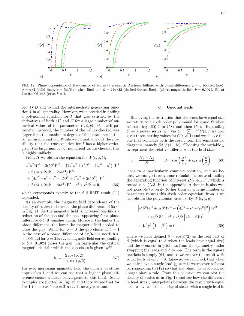
FIG. 12: Phase dependence of the density of states of a chaotic Andreev billiard with phase difference φ = 0 (dotted line),φ = π/2 (solid line), φ = 5π/6 (dashed line) and φ = 21π/22 (dashed dotted line). (a) At magnetic field b = 0.1024, (b) atb = 0.4096 and (c) at b = 1.

Sec. IVB and to find the intermediate generating func-tion I in all generality. However, we succeeded in findinga polynomial equation for I that was satisfied by thederivatives of both rH and G for a large number of nu-merical values of the parameters (ǫ, φ, b). For each pa-rameter involved, the number of the values checked waslarger than the maximum degree of the parameter in theconjectured equation. While we cannot rule out the pos-sibility that the true equation for I has a higher order,given the large number of numerical values checked thisis highly unlikely.From H we obtain the equation for W (ǫ, φ, b),

b2β2W 6 − 2ǫbβ2W 5 +(

2b2β2 + ǫ2β2 − 4bβ2 − b2)

W 4

+ 2(

ǫb+ 2ǫβ2 − 2ǫbβ2)

W 3

+(

4β2 − b2 − ǫ2 − 4bβ2 + b2β2 + 2ǫ2β2)

W 2

+ 2(

ǫb+ 2ǫβ2 − ǫbβ2)

W − ǫ2 + ǫ2β2 = 0, (66)

which corresponds exactly to the full RMT result (11)expanded.As an example, the magnetic field dependence of the

density of states is shown at the phase difference of 5π/6in Fig. 11. As the magnetic field is increased one finds areduction of the gap and the peak appearing for a phasedifference φ > 0 vanishes again. Moreover the higher thephase difference, the lower the magnetic field needed toclose the gap. While for φ = 0 the gap closes at b = 1in the case of a phase difference of 5π/6 one needs b ≈0.4096 and for φ = 21π/22 a magnetic field correspondingto b ≈ 0.1024 closes the gap. In particular the criticalmagnetic field for which the gap closes is given by35

bc =2 cos (φ/2)

1 + cos (φ/2). (67)

For ever increasing magnetic field the density of statesapproaches 1 and we can see that a higher phase dif-ference causes a faster convergence to this limit. Someexamples are plotted in Fig. 12 and there we see that forb = 1 the curve for φ = 21π/22 is nearly constant.

C. Unequal leads

Removing the restriction that the leads have equal sizewe return to a sixth order polynomial for g and G whensubstituting (60) into (58) and then (59). ExpandingG as a power series in r via G =

∑

rn−1C(ǫ, φ, n) nowgives three starting values for C(ǫ, φ, 1) and we choose theone that coincides with the result from the semiclassicaldiagrams, namely ββ∗/ (1− iǫ). Choosing the variable yto represent the relative difference in the lead sizes

y =N1 −N2

N, β = cos

(

φ

2

)

+ iy sin

(

φ

2

)

, (68)

leads to a particularly compact solution, and as be-fore, we can go through our roundabout route of findingthe generating function of interest H(ǫ, φ, y, r), which isrecorded as (A.3) in the appendix. Although it also wasnot possible to verify (other than at a large number ofparameter values) this sixth order equation, from it wecan obtain the polynomial satisfied by W (ǫ, φ, y):

[

ǫ2β2W 4 + 4ǫβ2W 3 +(

4β2 − ǫ2 + 2ǫ2β2)

W 2

+ 4ǫβ2W − ǫ2 + ǫ2β2]

(2 + ǫW )2

+ 4ǫ2y2(

1− β2)

= 0, (69)

where we have defined β = cos(φ/2) as the real part ofβ (which is equal to β when the leads have equal size)and the evenness in y follows from the symmetry underswapping the leads and φ to −φ. The term in the squarebrackets is simply (64) and so we recover the result withequal leads when y = 0. Likewise we can check that whenwe only have a single lead (y = ±1) we recover a factorcorresponding to (12) so that the phase, as expected, nolonger plays a role. From this equation we can plot thedensity of states as in Fig. 13 and see how the differencein lead sizes y interpolates between the result with equalleads above and the density of states with a single lead in

16

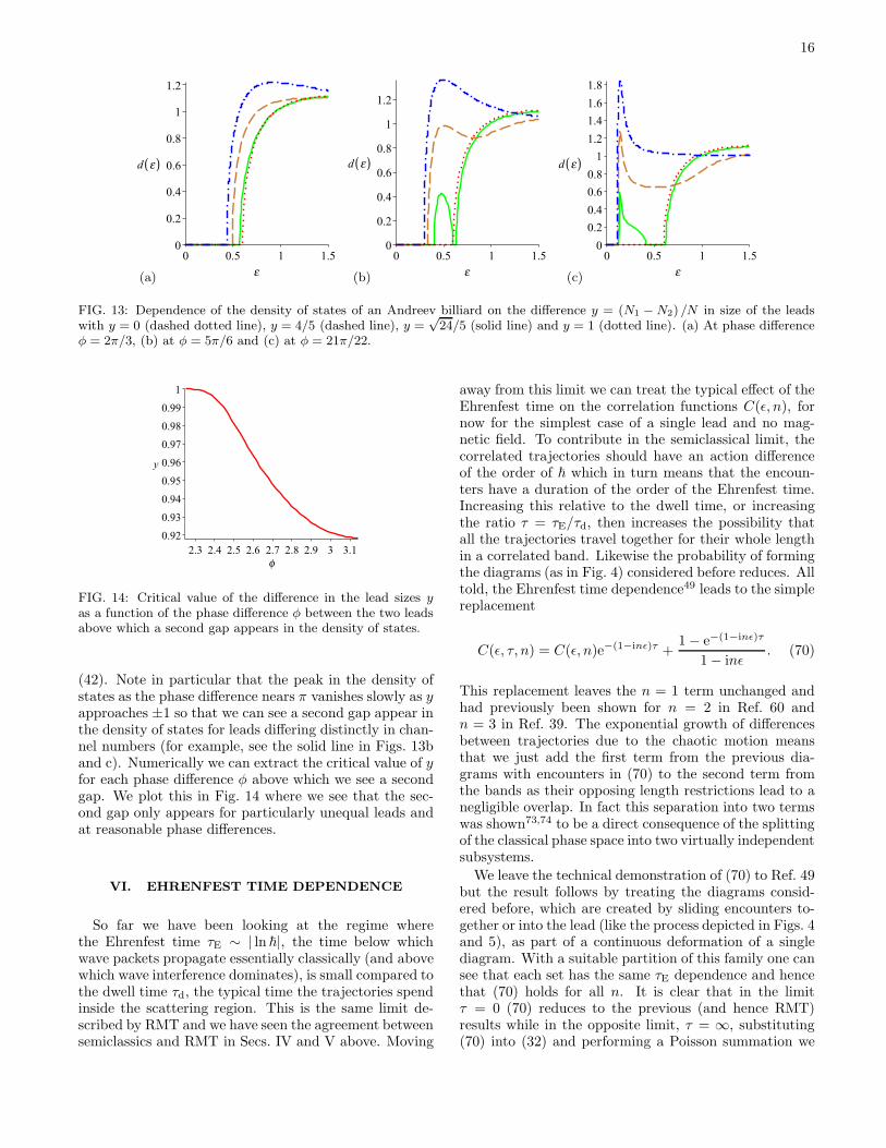
(a) (b) (c)

FIG. 13: Dependence of the density of states of an Andreev billiard on the difference y = (N1 −N2) /N in size of the leadswith y = 0 (dashed dotted line), y = 4/5 (dashed line), y =

√24/5 (solid line) and y = 1 (dotted line). (a) At phase difference

φ = 2π/3, (b) at φ = 5π/6 and (c) at φ = 21π/22.

FIG. 14: Critical value of the difference in the lead sizes yas a function of the phase difference φ between the two leadsabove which a second gap appears in the density of states.

(42). Note in particular that the peak in the density ofstates as the phase difference nears π vanishes slowly as yapproaches ±1 so that we can see a second gap appear inthe density of states for leads differing distinctly in chan-nel numbers (for example, see the solid line in Figs. 13band c). Numerically we can extract the critical value of yfor each phase difference φ above which we see a secondgap. We plot this in Fig. 14 where we see that the sec-ond gap only appears for particularly unequal leads andat reasonable phase differences.

VI. EHRENFEST TIME DEPENDENCE

So far we have been looking at the regime wherethe Ehrenfest time τE ∼ | ln ~|, the time below whichwave packets propagate essentially classically (and abovewhich wave interference dominates), is small compared tothe dwell time τd, the typical time the trajectories spendinside the scattering region. This is the same limit de-scribed by RMT and we have seen the agreement betweensemiclassics and RMT in Secs. IV and V above. Moving

away from this limit we can treat the typical effect of theEhrenfest time on the correlation functions C(ǫ, n), fornow for the simplest case of a single lead and no mag-netic field. To contribute in the semiclassical limit, thecorrelated trajectories should have an action differenceof the order of ~ which in turn means that the encoun-ters have a duration of the order of the Ehrenfest time.Increasing this relative to the dwell time, or increasingthe ratio τ = τE/τd, then increases the possibility thatall the trajectories travel together for their whole lengthin a correlated band. Likewise the probability of formingthe diagrams (as in Fig. 4) considered before reduces. Alltold, the Ehrenfest time dependence49 leads to the simplereplacement

C(ǫ, τ, n) = C(ǫ, n)e−(1−inǫ)τ +1− e−(1−inǫ)τ

1− inǫ. (70)

This replacement leaves the n = 1 term unchanged andhad previously been shown for n = 2 in Ref. 60 andn = 3 in Ref. 39. The exponential growth of differencesbetween trajectories due to the chaotic motion meansthat we just add the first term from the previous dia-grams with encounters in (70) to the second term fromthe bands as their opposing length restrictions lead to anegligible overlap. In fact this separation into two termswas shown73,74 to be a direct consequence of the splittingof the classical phase space into two virtually independentsubsystems.

We leave the technical demonstration of (70) to Ref. 49but the result follows by treating the diagrams consid-ered before, which are created by sliding encounters to-gether or into the lead (like the process depicted in Figs. 4and 5), as part of a continuous deformation of a singlediagram. With a suitable partition of this family one cansee that each set has the same τE dependence and hencethat (70) holds for all n. It is clear that in the limitτ = 0 (70) reduces to the previous (and hence RMT)results while in the opposite limit, τ = ∞, substituting(70) into (32) and performing a Poisson summation we

17

(a) (b)

FIG. 15: (a) Density of states for τ = τE/τd = 2 (solid line), along with the BS (dashed) limit τ → ∞ and the RMT (dotted)limit τ = 0, showing a second gap just below ǫτ = π. (b) Ehrenfest time related 2π/τ -periodic oscillations in the density ofstates after subtracting the BS curve.

(a) (b)

FIG. 16: (a) Width (and end point) of the first gap and (b)width of the second gap as a function of τ .

obtain the Bohr-Sommerfeld (BS)29 result

dBS(ǫ) =(π

ǫ

)2 cosh(π/ǫ)

sinh2(π/ǫ). (71)

This result was previously found semiclassically byRef. 30 and corresponds to the classical limit of bandsof correlated trajectories.For arbitrary Ehrenfest time dependence we simply

substitute the two terms in (70) into (32). With thesecond term we include 1 − (1 + τ)e−τ from the con-stant term (this turns out to simplify the expressions)and again perform a Poisson summation to obtain

d2(ǫ, τ) = 1− (1 + τ)e−τ (72)

+ 2Im

∞∑

n=1

(−1)n

n

∂

∂ǫ

(

1− e−(1−inǫ)τ

1− inǫ

)

= dBS(ǫ)

− exp

(

−2πk

ǫ

)(

dBS(ǫ) +2k(π/ǫ)2

sinh(π/ǫ)

)

,

where k = ⌊(ǫτ + π)/(2π)⌋ involves the floor function,and we see that this function is zero for ǫτ < π.

Of course the first term in (70) also contributes andwhen we substitute into (32) we obtain two further termsfrom the energy differential. These however may be writ-ten, using our semiclassical generating functions, as

d1(ǫ, τ) = e−τ[

1− 2Re eiǫτH(ǫ,−eiǫτ)]

(73)

+ τe−τ[

1− 2Re eiǫτG(ǫ,−eiǫτ )]

.

Because G and H are given by cubic equations, we canwrite this result explicitly as

d1(ǫ, τ) =

√3e−τ

6ǫRe [Q+(ǫ, τ) −Q−(ǫ, τ)] (74)

+

√3τe−τ

6Re [P+(ǫ, τ)− P−(ǫ, τ)] ,

where

Q±(ǫ, τ) =

[

8− 24ǫ (1− cos(ǫτ))

sin(ǫτ)− 24ǫ2

− 24ǫ2 (1− cos(ǫτ))

sin2(ǫτ)+

6ǫ3 (1− cos(ǫτ))

sin(ǫτ)

+2ǫ3(

2− 3 cos(ǫτ) + cos3(ǫτ))

sin3(ǫτ)

± 6ǫ√3D (1− cos(ǫτ))

sin2(ǫτ)

]13

, (75)

P±(ǫ, τ) =

[

36ǫ

(1 + cos(ǫτ))2 − 9ǫ2 sin(ǫτ)

(1 + cos(ǫτ))3 (76)

+ǫ3

(1 + cos(ǫτ))3± 3

√3D

(1 + cos(ǫτ))2

]13

.

These all involve the same discriminant D and so thedifferences in (74) are only real (and hence d1(ǫ, τ) itself

18

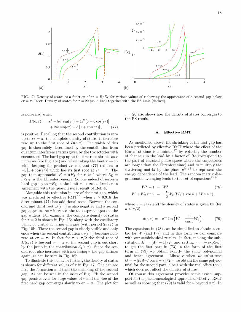
(a) (b)

FIG. 17: Density of states as a function of ǫτ = E/EE for various values of τ showing the appearance of a second gap belowǫτ = π. Inset: Density of states for τ = 20 (solid line) together with the BS limit (dashed).

is non-zero) when

D(ǫ, τ) = ǫ4 − 8ǫ3 sin(ǫτ) + 4ǫ2 [5 + 6 cos(ǫτ)]

+ 24ǫ sin(ǫτ) − 8 [1 + cos(ǫτ)] , (77)

is positive. Recalling that the second contribution is zeroup to ǫτ = π, the complete density of states is thereforezero up to the first root of D(ǫ, τ). The width of thisgap is then solely determined by the contribution fromquantum interference terms given by the trajectories withencounters. The hard gap up to the first root shrinks as τincreases (see Fig. 16a) and when taking the limit τ → ∞while keeping the product ǫτ constant (77) reduces to−8 [1 + cos(ǫτ)] which has its first root at ǫτ = π. Thegap then approaches E = πEE for τ ≫ 1 where EE =~/2τE is the Ehrenfest energy. So one indeed observes ahard gap up to πEE in the limit τ → ∞ at fixed ǫτ inagreement with the quasiclassical result of Ref. 40.Alongside this reduction in size of the first gap, which

was predicted by effective RMT13, when τ ≥ 0.916 thediscriminant (77) has additional roots. Between the sec-ond and third root D(ǫ, τ) is also negative and a secondgap appears. As τ increases the roots spread apart so thegap widens. For example, the complete density of statesfor τ = 2 is shown in Fig. 15a along with the oscillatorybehavior visible at larger energies (with period 2π/τ) inFig. 15b. There the second gap is clearly visible and onlyends when the second contribution d2(ǫ, τ) becomes non-zero at ǫτ = π. In fact for τ > π/2 the third root ofD(ǫ, τ) is beyond ǫτ = π so the second gap is cut shortby the jump in the contribution d2(ǫ, τ). Since the sec-ond root also increases with increasing τ the gap shrinksagain, as can be seen in Fig. 16b.To illustrate this behavior further, the density of states

is shown for different values of τ in Fig. 17. One can seefirst the formation and then the shrinking of the secondgap. As can be seen in the inset of Fig. 17b the secondgap persists even for large values of τ and the size of thefirst hard gap converges slowly to ǫτ = π. The plot for

τ = 20 also shows how the density of states converges tothe BS result.

A. Effective RMT

As mentioned above, the shrinking of the first gap hasbeen predicted by effective RMT where the effect of theEhrenfest time is mimicked37 by reducing the numberof channels in the lead by a factor eτ (to correspond tothe part of classical phase space where the trajectoriesare longer than the Ehrenfest time) and to multiply thescattering matrix by the phase eiǫτ/2 to represent theenergy dependence of the lead. The random matrix dia-grammatic averaging leads to the set of equations13,44

W 2 + 1 = W 22 (78)

W +W2 sinu = − ǫ

2W2 (W2 + cosu+W sinu) ,

where u = ǫτ/2 and the density of states is given by (foru < π/2)

d(ǫ, τ) = −e−τ Im(

W − u

cosuW2

)

. (79)

The equations in (78) can be simplified to obtain a cu-bic for W (and W2) and in this form we can comparewith our semiclassical results. In fact, making the sub-stitution H = [iW − 1] /2r and setting r = − exp(iǫτ)to get the first part in (73) in the form of the firstterm in (79) we obtain exactly the same polynomialand hence agreement. Likewise when we substituteG = − [iuW2/ cosu+ τ ] /2rτ we obtain the same polyno-mial for the second part, albeit with the real offset tanuwhich does not affect the density of states.Of course this agreement provides semiclassical sup-

port for the phenomenological approach of effective RMTas well as showing that (79) is valid for u beyond π/2. In

19

(a) (b) (c)

FIG. 18: Density of states for τ = 2 (solid line) along with the τ = 0 (dotted) and τ = ∞ (dashed) limits for a chaotic Andreevbilliard with phase difference (a) φ = π/18, (b) φ = 5π/6 and (c) φ = π.

principle then the second gap could also have been foundusing effective RMT, but of course effective RMT missesthe second contribution to the density of states d2(ǫ, τ).This contribution turns out to be straightforward to ob-tain semiclassically, and can be compared to the bandstreated in Ref. 40.

B. Two superconducting leads

If we include the effect of a symmetry breaking mag-netic field then, because of the way this affects the con-tribution of different sized encounters (as described inSec. IVD), such a simple replacement as in (70) no longerholds. This situation has however been treated using ef-fective RMT44 allowing them to also determine how thecritical magnetic field (at which the gap closes) dependson the Ehrenfest time. Without the simple replacementof the magnetic field dependent correlations functions weare currently unable to confirm this result semiclassically.But if we look at two superconducting leads (for simplic-ity of equal size) at different phase this effect can beincluded in the channel sum and treated as above (theeffective RMT result can be found by a simple modifica-tion of the treatment in Ref. 44). Important to rememberis that the second part (of (70)) corresponds to bands oftrajectories that are correlated for their whole length andso they all start and end together (in the same leads).Therefore the second contribution has to be multipliedby [1 + cos(nφ)]/2 leading to

C(ǫ, φ, τ, n) = C(ǫ, φ, n)e−(1−inǫ)τ (80)

+1 + cos(nφ)

2

1− e−(1−inǫ)τ

1− inǫ.

The first part of the density of states for non zero Ehren-fest time then remains as in (73) but with G(ǫ, r) andH(ǫ, r) replaced by G(ǫ, φ, r) and H(ǫ, φ, r), respectively.The second contribution in this case however may bewritten as the average of the φ = 0 contribution and

a contribution with the full phase difference φ,

d2(ǫ, φ, τ) =1

2[d′2(ǫ, 0, τ) + d′2(ǫ, φ, τ)] . (81)

Here d′2(ǫ, φ, τ) may be again written as the sum of theτ = ∞ result

d′(1)2 (ǫ, φ, τ) =

π

2ǫ2 sinh2 (π/ǫ)(82)

×[

(π + 2πk1 − φ) cosh

(

π − 2πk1 + φ

ǫ

)

+ (π − 2πk1 + φ) cosh

(

π + 2πk1 − φ

ǫ

)]

,

and some correction

d′(2)2 (ǫ, φ, τ) = − π

2ǫ2 sinh2 (π/ǫ)(83)

×{[

π cosh(π

ǫ

)

+ (2πk2 − φ) sinh(π

ǫ

)]

e−2πk2−φ

ǫ

+[

π cosh(π

ǫ

)

+ (2πk3 + φ) sinh(π

ǫ

)]

e−2πk3+φ

ǫ

}

,

with k1 = ⌊(π + φ) /(2π)⌋, k2 = ⌊(ǫτ + π + φ) /(2π)⌋ andk3 = ⌊(ǫτ + π − φ) /(2π)⌋. Since the ki and φ only occurin the combinations 2πk1−φ, 2πk2−φ and 2πk3+φ it isobvious that these contributions have oscillations in thephase φ with period 2π. It can also be easily seen thatfor φ = 0 the previous result for the density of states inthe Ehrenfest regime is reproduced.With |φ| < π we have k1 = k2 = k3 = 0 for ǫτ <

π − |φ|. Therefore one again sees that d2 = 0 as long

as ǫτ < π − |φ|. The first part d′(1)2 equals the Bohr-

Sommerfeld result (71), so in the limit τ = ∞ this resultis reproduced again. The oscillations in ǫ seen in theφ = 0 case which have a period of 2π/τ can still be seendue to the fact that the φ = 0 result enters d2(ǫ, φ, τ)even if φ 6= 0. However one gets additional (but smaller)steps at energies satisfying ǫ = [(2m − 1)π ∓ φ]/τ forinteger m.We plot the density of states for τ = 2, along with the

τ = 0 and τ = ∞ limits in Fig. 18 for different values of

20

(a) (b)

FIG. 19: Density of states for τ = 1/2 (dotted line), τ = 1 (dashed) and τ = 2 (solid) showing the phase dependent jumps forphase difference (a) φ = π/18 and (b) φ = 5π/6.

the phase difference. We can see that as the phase differ-ence increases the second intermediate gap (c.f. Fig. 15a)shrinks quickly. The reason for this shrinking is twofold:On the one hand, the gap in the RMT-like contributionshrinks, and on the other hand, the second contributionis zero only up to ǫτ = π − |φ|. Moreover if φ → π themodified correlation function tends to zero so the densityof states converges to (1 + τ)e−τ + d2(ǫ, τ). For a finerlook at the Ehrenfest time dependence and the phase de-pendent jumps we plot the density of states for τ = 1/2,1 and 2 for phases φ = π/18 and 5π/6 in Fig. 19.

VII. CONCLUSIONS

From the semiclassical treatment of the density ofstates of chaotic Andreev billiards we have seen how finecorrelations between ever larger sets of classical trajec-tories lead to the interference effects which cause a hardgap in the density of states. This treatment (c.f. thereservations in Ref. 38) builds on the recent advances inidentifying55, codifying56,57 and generating47 the semi-classical contributions, and, because of the slow conver-gence of the expansion for the density of states in (15),relies on the ability to treat correlations between n tra-jectories for essentially all n. The correlations betweenthese trajectories, encoded in encounter regions wherethey differ slightly, are represented by simple (tree) dia-grams. These diagrams are related to those that appearfor the conductance56 say where for increasing n theycause ever decreasing (in inverse channel number) cor-rections; here though they all contribute with roughlythe same (slowly decreasing) importance. It is becausewe need to treat all orders that Andreev billiards are sointeresting and the resultant effects so large.Along with obtaining the minigap, found by RMT27,

for a billiard with a single lead, we could also obtain thefull result for the density of states of an Andreev billiard

with two superconducting leads at phase difference φ,treated using RMT in Ref. 35. The semiclassical pathsthat connect the two leads accumulate phases e±iφ andcause the gap to shrink with increasing phase difference.It was also possible to treat the effect of a time rever-sal symmetry breaking magnetic field b, considered withRMT in Ref. 35, which makes the formation of the clas-sical trajectory sets, traversed in opposite directions byan electron and a hole, less likely. This in turn leads toa reduction of the minigap and a smoothing of the den-sity of states, especially for large phase differences φ. Wehave found that in the limits φ → π and b → ∞ quantumeffects vanish and the density of states becomes identicalto the density of states of the isolated billiard.

The agreement shown here between the semiclassicaland the RMT results may lead one to wonder about thedeeper connections between the two methods. Indeed thediagrammatic methods69 used in RMT, which also use re-cursion relations over planar diagrams, bear some resem-blance to the tree recursions here, but unfortunately anycorrespondence between the two is somewhat obscuredby the transformation from the generating function G tothe generating function H . It is also worth pointing outthat our semiclassical treatment (with its inherent semi-classical limits) gives us access to the typical and univer-sal density of states of chaotic systems. However therecan be further effects that change the shape of the den-sity of states, for example scarring75, classical Lyapunovexponent fluctuations76 and disorder77.

Of course all our results in this paper (and the RMTones27,35) are only valid to leading order in inverse chan-nel number. With the formalism shown in this paper, togo to subleading order we only require a way of generat-ing the possible semiclassical diagrams. The contributionof each56,57 and how they affect the density of states isknown in principle, but the key problem is that the struc-ture we used here breaks down, namely that in the treerecursions when we cut a rooted plane tree at a node we

21

created additional rooted plane trees47. How to treat thepossible diagrams which include closed loops etc, thoughgenerated for n = 1 in Ref. 56 and n = 2 in Ref. 57by cutting open closed periodic orbits, remains unclear.However the treatment for n = 1 and n = 2 makes it clearthat the diagrams that contribute at order (1/Nm, n) arerelated to those that contribute at order (1/Nm−1, n+1),raising the possibility of a recursive treatment startingfrom the leading order diagrams described here.Worth noting is that the semiclassical techniques we

used here are only valid up to the Heisenberg time, mean-ing that we have no access to the density of states on en-ergy scales of the order of the mean level spacing. Thoughfor ballistic transport the Heisenberg time is much longerthan the average dwell time (so the mean level spacingis much smaller than the Thouless energy) importantlythe RMT treatment78 shows that a microscopic gap per-sists in this regime even when the time reversal symme-try is completely broken (by the magnetic field say). Itmay be possible that applying the semiclassical treat-ment of times longer than the Heisenberg time for closedsystems79,80 to transport would allow one to access thisregime as well.In the opposite regime however, that of the Ehrenfest

time, semiclassics provides a surprisingly simple result49

allowing complete access to the crossover from the univer-sal RMT regime to the more classical Bohr-Sommerfeldregime. The gap shrinks due to the suppression of the for-mation of encounters while a new class of diagrams (cor-related bands) becomes possible. Interestingly the contri-bution from trajectories with encounters agrees exactlywith the results from effective RMT13, so our semiclas-sical result provides support for this phenomenologicalapproach. Of course effective RMT misses the bands ofcorrelated trajectories (c.f. those in Ref. 40) which com-bined with the other contribution lead to new effects,most notably a second gap in the density of states forintermediate Ehrenfest times.

Acknowledgments

The authors would like to thank I. Adagideli for usefulconversations and gratefully acknowledge the DeutscheForschungsgemeinschaft within GRK 638 (DW, KR) andFOR 760 (KR), the National Science Foundation un-der grant 0604859 (GB), CEA Eurotalent (CP) and theAlexander von Humboldt Foundation (JK, CP) for fund-ing.

Appendix: Further generating functions

The intermediate generating function I(ǫ, r) for the billiard with a single lead and no magnetic field in Sec. IVB isgiven by

1−[

(1− a)2+ 6r + (1 + a)

2r2]

I +[

4 (1− a)3 −

(

8 + 20a2 − a4)

r + 4 (1 + a)3r2]

rI2

+[

4 (1− a)3 −

(

16− 24a+ 44a2 − 8a3 − a4)

r + 2(

12 + 32a2 − a4)

r2

−(

16 + 24a+ 44a2 + 8a3 − a4)

r3 + 4 (1 + a)3r4]

rI3 = 0, (A.1)

where we set a = iǫ.

The generating function H(ǫ, φ, b, r) for the billiard with equal leads at phase difference φ and magnetic field b inSec. VB is given by

β2 −(

(1− a+ b)2 + r2 − 2r (1− a+ b)(

2β2 − 1)

)

H

− r[

(1− a+ b) (1− 3a+ 7b)− 2r(

1 + 5b+ b2 − (3 + 2b)a+ a2) (

2β2 − 1)

+ r2 (1− 2a+ 2b)]

H2

+ r2[

−b (19b+ 10) + 2a (9b+ 1)− 3a2 + 2r(

2b (3b+ 4)− 2a (4b+ 1) + 2a2) (

2β2 − 1)

+ r2(

−b (b + 6) + 2a (b+ 1)− a2)]

H3

− r3[

b (25b+ 4)− 14ab+ a2 − 2r(

b (13b+ 4)− 10ab+ a2) (

2β2 − 1)

+ r2(

b (5b+ 4)− 6ab+ a2)]

H4

− 4r4b[

4b− a− 2r (3b− a)(

2β2 − 1)

+ r2 (2b− a)]

H5

− 4r5b2[

1 + r2 − 2r(

2β2 − 1)]

H6 = 0, (A.2)

where we also used a = iǫ. For the billiard with unequal leads and no magnetic field in Sec. VC, the generating

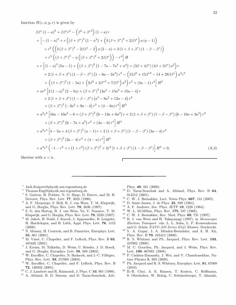
22

function H(ǫ, φ, y, r) is given by

ββ∗ (1− a)2 + ββ∗r2 −(

β2 + β∗2)

(1− a) r

+[

− (1− a)4+ r

(

(β + β∗)2 (

1− a3)

+(

3 (β + β∗)2+ 2ββ∗

)

a (a− 1))

+ r2((

3 (β + β∗)2 − 2ββ∗ − 2

)

a (2− a) + 2 (1 + β + β∗) (1− β − β∗))

+ r3(

(β + β∗)2 − a(

(β + β∗)2 + 2ββ∗))

− r4]

H

+ r[

(1− a)3(5a− 1) +

(

(β + β∗)2 (

1− 7a− 7a3 + a4)

+ (3β + 4β∗) (4β + 3β∗) a2)

r

+ 2 (1 + β + β∗) (1− β − β∗)(

1− 6a− 2a3)

r2 −(

15β2 + 15β∗2 − 14 + 28ββ∗)

a2r2

+(

(β + β∗)2 (1− 5a) +(

3β2 + 3β∗2 + 7ββ∗)

a2)

r3 + (4a− 1) r4]

H2

+ ar2[

2 (1− a)2(2− 5a) + (β + β∗)

2 (4a3 − 15a2 + 15a− 4

)

r

+ 2 (1 + β + β∗) (1− β − β∗)(

a3 − 8a2 + 12a− 4)

r2

+ (β + β∗)2 (−3a2 + 9a− 4

)

r3 + (4− 6a) r4]

H3

+ a2r3[

16a− 10a2 − 6 + (β + β∗)2(

6− 13a+ 6a2)

r + 2 (1 + β + β∗) (1− β − β∗)(

6− 10a+ 3a2)

r2

+ (β + β∗)2 (

6− 7a+ a2)

r3 + (4a− 6) r4]

H4

+ a3r4[

4− 5a+ 4 (β + β∗)2(a− 1) r + 2 (1 + β + β∗) (1− β − β∗) (3a− 4) r2

+ (β + β∗)2 (2a− 4) r3 + (4− a) r4]

H5

+ a4r5(

−1− r4 + r(

1 + r2)

(β + β∗)2+ 2r2 [1 + β + β∗) (1− β − β∗)

]

H6 = 0, (A.3)

likewise with a = iǫ.

∗ Jack.Kuipers@physik.uni-regensburg.de† Thomas.Engl@physik.uni-regensburg.de1 S. Gueron, H. Pothier, N. O. Birge, D. Esteve, and M. H.Devoret, Phys. Rev. Lett. 77, 3025 (1996).

2 A. F. Morpurgo, S. Holl, B. J. van Wees, T. M. Klapwijk,and G. Borghs, Phys. Rev. Lett. 78, 2636 (1997).

3 S. G. den Hartog, B. J. van Wees, Yu. V. Nazarov, T. M.Klapwijk, and G. Borghs, Phys. Rev. Lett. 79, 3250 (1997).

4 M. Jakob, H. Stahl, J. Knoch, J. Appenzeller, B. Lengeler,H. Hardtdegen, and H. Luth, Appl. Phys. Lett. 76, 1152(2000).

5 N. Moussy, H. Courtois, and B. Pannetier, Europhys. Lett.55, 861 (2001).

6 M. Vinet, C. Chapelier, and F. Lefloch, Phys. Rev. B 63,165420 (2001).

7 J. Eroms, M. Tolkiehn, D. Weiss, U. Rossler, J. D. Boeck,and G. Borghs, Europhys. Lett. 58, 569 (2002).

8 W. Escoffier, C. Chapelier, N. Hadacek, and J.-C. Villegier,Phys. Rev. Lett. 93, 217005 (2004).

9 W. Escoffier, C. Chapelier, and F. Lefloch, Phys. Rev. B72, 140502 (2005).

10 C. J. Lambert and R. Raimondi, J. Phys. C 10, 901 (1998).11 A. Altland, B. D. Simons, and D. Taras-Semchuk, Adv.

Phys. 49, 321 (2000).12 D. Taras-Semchuk and A. Altland, Phys. Rev. B 64,

014512 (2001).13 C. W. J. Beenakker, Lect. Notes Phys. 667, 131 (2005).14 D. Saint-James, J. de Phys. 25, 899 (1964).15 A. F. Andreev, Sov. Phys. JETP 19, 1228 (1964).16 W. L. McMillan, Phys. Rev. 175, 537 (1968).17 C. W. J. Beenakker, Rev. Mod. Phys. 69, 731 (1997).18 B. J. van Wees and H. Takayanagi (1997), in Mesoscopic

Electron Transport eds. L. L. Sohn, L. P. Kouwenhovenand G. Schon NATO ASI Series E345 Kluwer, Dordrecht.

19 V. A. Gopar, J. A. Mendez-Bermudez, and A. H. Aly,Phys. Rev. B 79, 245412 (2009).

20 R. S. Whitney and Ph. Jacquod, Phys. Rev. Lett. 103,247002 (2009).

21 M. C. Goorden, Ph. Jacquod, and J. Weiss, Phys. Rev.Lett. 100, 067001 (2008).

22 P. Cadden-Zimansky, J. Wei, and V. Chandrasekhar, Na-ture Physics 5, 393 (2009).

23 Ph. Jacquod and R. S. Whitney, Europhys. Lett. 91, 67009(2010).

24 B.-R. Choi, A. E. Hansen, T. Kontos, C. Hoffmann,S. Oberholzer, W. Belzig, C. Schonenberger, T. Akazaki,

23

and H. Takayanagi, Phys. Rev. B 72, 024501 (2005).25 J. Eroms and D. Weiss, Appl. Phys. A 89, 639 (2007).26 I. Kosztin, D. L. Maslov, and P. M. Goldbart, Phys. Rev.

Lett. 75, 1735 (1995).27 J. A. Melsen, P. W. Brouwer, K. M. Frahm, and C. W. J.

Beenakker, Europhys. Lett. 35, 7 (1996).28 A. Lodder and Y. V. Nazarov, Phys. Rev. B 58, 5783

(1998).29 H. Schomerus and C. W. J. Beenakker, Phys. Rev. Lett.

82, 2951 (1999).30 W. Ihra, M. Leadbeater, J. L. Vega, and K. Richter, Eur.

Phys. J. B 21, 425 (2001).31 W. Ihra and K. Richter, Physica E 9, 362 (2001).32 J. Cserti, A. Kormanyos, Z. Kaufmann, J. Koltai, and C. J.

Lambert, Phys. Rev. Lett. 89, 057001 (2002).33 I. Adagideli and P. M. Goldbart, Int. J. Mod. Phys. B 16,

1381 (2002).34 O. Zaitsev, J. Phys. A 39, L467 (2006).35 J. A. Melsen, P. W. Brouwer, K. M. Frahm, and C. W. J.

Beenakker, Phys. Scr. T69, 223 (1997).36 I. Adagideli and C. W. J. Beenakker, Phys. Rev. Lett. 89,

237002 (2002).37 P. G. Silvestrov, M. C. Goorden, and C. W. J. Beenakker,

Phys. Rev. Lett. 90, 116801 (2003).38 M. G. Vavilov and A. I. Larkin, Phys. Rev. B 67, 115335

(2003).39 P. W. Brouwer and S. Rahav, Phys. Rev. B 74, 085313

(2006).40 T. Micklitz and A. Altland, Phys. Rev. Lett. 103, 080403

(2009).41 Ph. Jacquod, H. Schomerus, and C. W. J. Beenakker,

Phys. Rev. Lett. 90, 207004 (2003).42 A. Kormanyos, Z. Kaufmann, C. J. Lambert, and J. Cserti,

Phys. Rev. B 70, 052512 (2004).43 H. Schomerus and Ph. Jacquod, J. Phys. A 38, 10663

(2005).44 M. C. Goorden, Ph. Jacquod, and C. W. J. Beenakker,

Phys. Rev. B 72, 064526 (2005).45 J. Kuipers, D. Waltner, C. Petitjean, G. Berkolaiko, and

K. Richter, Phys. Rev. Lett. 104, 027001 (2010).46 C. W. J. Beenakker, Phys. Rev. Lett. 67, 3836 (1991).47 G. Berkolaiko, J. M. Harrison, and M. Novaes, J. Phys. A

41, 365102 (2008).48 G. Berkolaiko and J. Kuipers, J. Phys. A 43, 035101

(2010).49 D. Waltner, J. Kuipers, and K. Richter, Phys. Rev. B 83,

195315 (2011).50 P. W. Brouwer and C. W. J. Beenakker, J. Math. Phys.

37, 4904 (1996).51 W. H. Miller, Adv. Chem. Phys. 30, 77 (1975).52 E. Akkermans, A. Auerbach, J. E. Avron, and B. Shapiro,

Phys. Rev. Lett. 66, 76 (1991).53 E. Doron and U. Smilansky, Phys. Rev. Lett. 68, 1255

(1992).54 C. H. Lewenkopf and R. O. Vallejos, Phys. Rev. E 70,

036214 (2004).55 K. Richter and M. Sieber, Phys. Rev. Lett. 89, 206801

(2002).56 S. Heusler, S. Muller, P. Braun, and F. Haake, Phys. Rev.

Lett. 96, 066804 (2006).57 S. Muller, S. Heusler, P. Braun, and F. Haake, New J.

Phys. 9, 12 (2007).58 K. Richter, Semiclassical theory of mesoscopic quantum

systems (Springer, Berlin, 2000).59 P. Braun, S. Heusler, S. Muller, and F. Haake, J. Phys. A

39, L159 (2006).60 R. S. Whitney and Ph. Jacquod, Phys. Rev. Lett. 96,

206804 (2006).61 A. Lassl (2003), Diplomarbeit Universitat Regensburg.62 M. Sieber and K. Richter, Phys. Scr. T90, 128 (2001).63 D. Spehner, J. Phys. A 36, 7269 (2003).64 M. Turek and K. Richter, J. Phys. A 36, L455 (2003).65 P. W. Brouwer and S. Rahav, Phys. Rev. B 74, 075322

(2006).66 W. T. Tutte, Am. Math. Mon. 71, 272 (1964).67 J. H. Hannay and A. M. Ozorio de Almeida, J. Phys. A

17, 3429 (1984).68 R. P. Stanley, Enumerative Combinatorics, Volume 2

(Cambridge University Press, Cambridge, 2001).69 P. W. Brouwer and C. W. J. Beenakker, Chaos, Solitons

& Fractals 8, 1249 (1997).70 K. Saito and T. Nagao, Phys. Lett. A 352, 380 (2006).71 T. Nagao, P. Braun, S. Muller, K. Saito, S. Heusler, and

F. Haake, J. Phys. A 40, 47 (2007).72 J. Kuipers and M. Sieber, J. Phys. A 40, 935 (2007).73 R. S. Whitney and Ph. Jacquod, Phys. Rev. Lett. 94,

116801 (2005).74 Ph. Jacquod and R. S. Whitney, Phys. Rev. B 73, 195115

(2006).75 A. Kormanyos and H. Schomerus, Phys. Rev. Lett. 97,

124102 (2006).76 P. G. Silvestrov, Phys. Rev. Lett. 97, 067004 (2006).77 F. Libisch, J. Moller, S. Rotter, M. G. Vavilov, and

J. Burgdorfer, Europhys. Lett. 82, 47006 (2008).78 K. M. Frahm, P. W. Brouwer, J. A. Melsen, and C. W. J.

Beenakker, Phys. Rev. Lett. 76, 2981 (1996).79 S. Heusler, S. Muller, A. Altland, P. Braun, and F. Haake,

Phys. Rev. Lett. 98, 044103 (2007).80 S. Muller, S. Heusler, A. Altland, P. Braun, and F. Haake,

New J. Phys. 11, 103025 (2009).