Electronic Realization of Chaotic Differential Equations

Chris Parker, Travis Petersen, Eric Kangas, Sami Abdul-Wahid, Evan Masters

Faculty Advisor: Dr. Michael Braunstein

Abstract: Understanding the fundamental principles that govern chaotic behavior is sought not only for its inherent educational value, but for its applications in physics, information theory, meteorology, biology and mathematics. J.C. Sprott has reported on a class of chaotic differential equations that can, in principle, be simply realized using discrete electronic components. These circuits can be used to investigate chaotic behavior in a simple system. We will present computational and experimental data collected from one simple chaotic circuit. Our computational results include eigenvalues and eigenvectors of the Jacobian, return maps, largest Lyapunov exponents and the numerical approximation of solutions to the differential equation utilized. Our data include output voltages at different points in the circuit representing the phase space behavior of the system. A comparison between the model and collected experimental data will be provided to analyze the realization of the nonlinear differential equation.

IntroductionAlthough there exists no universal consensus on an exact definition, chaos is usually

described as a deterministic system that displays aperiodic, long-term bounded behavior with sensitive dependence on initial conditions[1]. An interesting class of chaotic differential equations has been found that can be modeled by simple electronic circuits[2], and one of these is the focus of this project. The general form of these equations is given by:

Cxfxxxx ++++=••••••

)(γβα ,

where the dots represent derivatives with respect to time, α, β, γ, and C are real constants, and f(x) is a nonlinear function. Because these systems have a dependence on the third time derivative of the variable x they are identified as jerk functions. When realizing these equations electronically, values of x and its derivatives are characterized by voltages at specific points in the circuit.

We designed and constructed several implementations of circuits for one of these equations:

2xxxxx +−−−=••••••

α , with a control parameter (α) corresponding to an adjustable electronic component that could be varied to produce a wide range of values. For certain values of the control parameter, the output values vary periodically with time, but if the control parameter is set to a value in the chaotic range, the output values vary in an apparently chaotic manner.

With these circuits, we investigated qualitative and quantitative behaviors of the system as a function of the control parameter and compared these behaviors to numerical models.

Methods

Designing the Circuit

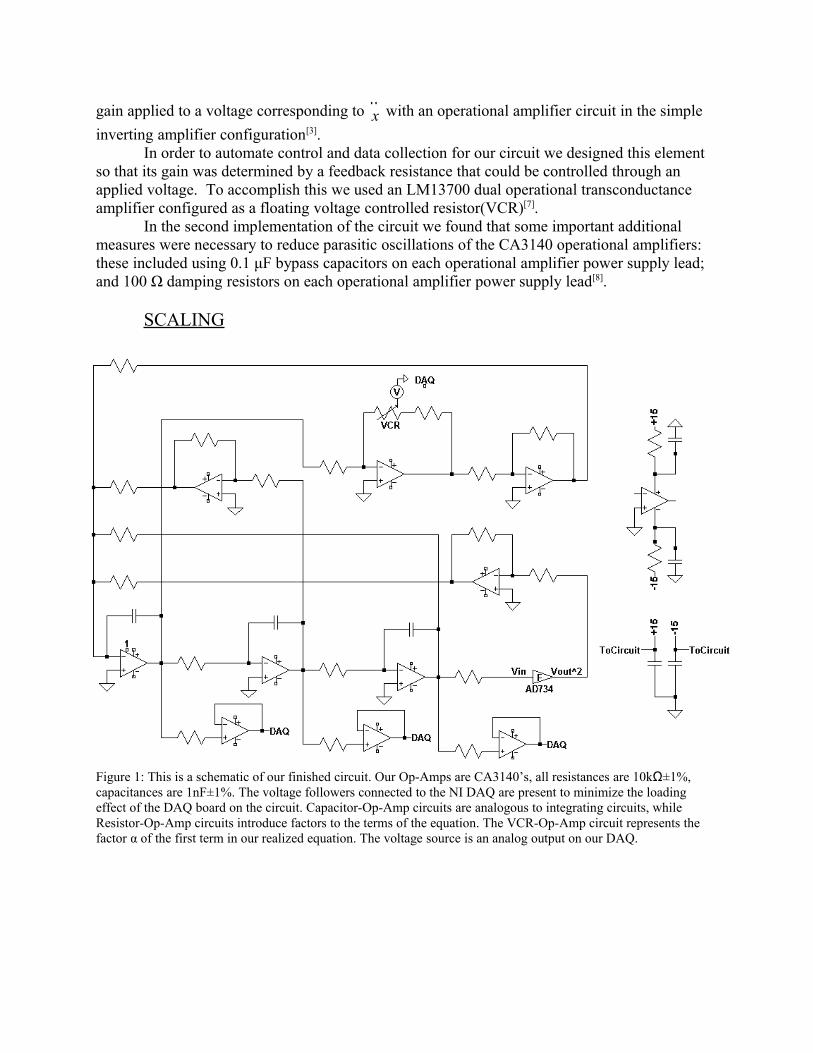
Recognizing that a simple implementation of an integrating circuit consists of a signal applied to the inverting input of an operational amplifier through a resistor, and a feedback capacitor[3], we designed our circuit by applying the integrator-adder-gain block diagram approach. This allowed us to systematically assemble a circuit using simple operational-amplifier circuits to represent different elements of the equation to be realized. [Figure 1] shows our final circuit. Early on in the circuit design, we decided to use a variable resistance to realize the control parameter, α.

All of the circuits that were used in this research were constructed (breadboarded) on E&L Instruments C.A.D.E.T.™ electronics trainers. In an initial implementation, the components we used were μA741 [4] operational amplifiers and lower accuracy (5%) resistors and ceramic disc capacitors. In a second implementation, intended to improve the correspondence between the numerical model and the electronic circuit, we used CA3140 operational amplifiers, which have significantly higher input impedance than the μA741 operational amplifiers, and higher accuracy (1%) resistors and polypropylene capacitors[5].

A fundamental aspect of a continuous chaotic system is that it must contain a non-linear term. The x2 term in Equation 2 is the non-linear term for our system and we implemented this in our circuit using an AD734, 10 MHz, 4-Quadrant Multiplier/Divider integrated circuit in the Basic Multiplier Circuit configuration[6]. The control parameter, α, was implemented through a

gain applied to a voltage corresponding to ••x with an operational amplifier circuit in the simple

inverting amplifier configuration[3]. In order to automate control and data collection for our circuit we designed this element

so that its gain was determined by a feedback resistance that could be controlled through an applied voltage. To accomplish this we used an LM13700 dual operational transconductance amplifier configured as a floating voltage controlled resistor(VCR)[7].

In the second implementation of the circuit we found that some important additional measures were necessary to reduce parasitic oscillations of the CA3140 operational amplifiers: these included using 0.1 μF bypass capacitors on each operational amplifier power supply lead; and 100 Ω damping resistors on each operational amplifier power supply lead[8].

SCALING

Figure 1: This is a schematic of our finished circuit. Our Op-Amps are CA3140’s, all resistances are 10kΩ±1%, capacitances are 1nF±1%. The voltage followers connected to the NI DAQ are present to minimize the loading effect of the DAQ board on the circuit. Capacitor-Op-Amp circuits are analogous to integrating circuits, while Resistor-Op-Amp circuits introduce factors to the terms of the equation. The VCR-Op-Amp circuit represents the factor α of the first term in our realized equation. The voltage source is an analog output on our DAQ.

Data Collection Methods

Data was collected using the National Instruments 6251 M-Series Data Acquisition hardware (DAQ). This DAQ allowed us to incorporate several features of automation into our data collection, allowing us to develop a numerical map of the phase space of our circuit. Our control system on the DAQ, the VCR, was connected to an analog voltage output on the DAQ. We then wrote a LabVIEW program which enables us to iteratively sample sets of ordered triplets over a user-determined portion of the control voltage range.

The purpose of the LabVIEW program is to allow the data collectors to input a desired number of “slices” of the phase space of the circuit. The program then calculates the optimal step size for the VCR's control voltage and automatically begins collecting and saving data sets to a user-defined directory. These data sets correspond to phase plots of the three voltages of interest in our circuit at specific values of the control parameter. Each data set is saved when it is collected, then tagged with the analog output voltage at which it was collected.

This allows us to approximate the control parameter value at which this slice of the phase space should appear in our model. With this information it becomes possible to make a comparison between the phase space of our model and the phase space of our system.

Modeling Solutions to the Differential Equation

To understand the behavior of this equation a numerical solution to this differential equation (DE) was sought, along with a phase space diagram that plotted the solution of x versus the solution of one of the derivatives (

•••xx, ). To find a solution to this DE, a numerical

approximation was used that utilized an Adams predictor-corrector method. Mathematica 6 was used to this end, as its built in functions are some of the most powerful tools when performing numerical approximations of DEs. To test the chaotic behavior of this equation, the solution was sought with the hopes of finding both periodic and non-periodic solutions.

This function utilized initial conditions given by Sprott and enabled the investigation of the behavior of the solution under different values of the control parameter, listed here as a (α as stated above). Additionally, double precision and accuracy were used according to the suggestion of previous work done on Mathematica involving chaotic systems[9]. The precision of the internal computations was increased dramatically from the automatic value in order to reduce the uncertainty associated with our numerical approximations. The solution was most easily observable when plotted over time. Because Mathematica gives numerical solutions in the form of an interpolating function, a substitution must be made in the plot function in order to extrapolate the data of the interpolation function. As shown in [Figure 2], the Plot function was used with a substitution of the interpolation function and the resulting plot suggests a periodic behavior.

20 40 60 80 100

-0.5

-0.25

0.25

0.5

0.75

1

Figure 2: A plot of computational data created in Mathematica.

To obtain a phase space diagram, a similar method was utilized. First, a solution was found in the same manner as described above. The solution to the first derivative of the numerical approximation was then found and both solutions were plotted against each other using a parametric plot. Maintaining the control parameter at 0.5, a phase space diagram could be obtained which was easily comparable with experimental data taken using an oscilloscope. It is important to note, however, that the control parameter could be varied in this process to make phase space diagrams with any control parameter or scaling factor in the DE.

Yet, in order to ensure that chaotic behavior was taking place, the calculation of the (largest) Lyapunov exponent was needed. The J.C. Sprott paper[2] provides a numerical value of the Lyapunov exponent for this DE using the initial conditions stated earlier[1]. Independent verification of this exponent was sought to ensure an understanding for this characteristic of a chaotic system as well as to determine the chaotic behavior of the DE chosen. Calculation of the Lyapunov exponent was done using a method outlined by Sprott himself.

First, the third order nonlinear differential equation being used had to be transformed into three first order differential equations. The solutions to these differential equations were treated as components of a three dimensional vector (R) that was treated as the orbit. Initial conditions were chosen from values given in Sprott’s paper and another R vector (ΔR) was chosen with initial condition 10-10 different than R. Numerical solutions to these orbits were found for a small time step, and the vector’s final positions were measured. The difference between their solutions from a small change in the initial conditions is the important quantity to be determined.

The positions of the ΔR orbit were then changed in such a way as to keep the two orbits close while letting the direction orient to that of maximum expansion[1]. This process was iterated 7 x 106 times, with a time step of .01s per iteration, while calculating a running sum of ln(ΔRn/ΔR0) (where ΔRn was the magnitude of the change calculated in the nth step while ΔR0 was the magnitude of the change in the first iteration). The average of this yielded the Lyapunov exponent, when divided by the time step.

Characterization of Model using a Return Map

The return map is the first step in creating a bifurcation diagram for our system. It can also be used to determine whether or not the system is behaving periodically, based on the level of continuity between points in the map. We used Mathematica 6 to perform computations in this process. To start the process for plotting the return map a fractional value of the control parameterwas determined for the numerical solution to the DE. Then, we needed to find the roots of the DE for the determined value of the control parameter and within a specific period of time.

In the process of finding the roots there a number of extraneous maximum values appeared that needed to be filtered out. A Mathematica 6 function was used to set a precision of 6 in this evaluation since some of the calculated maxima were close to the same value. This precision appeared to be the point at which the maxima and minima started to diverge from each other in computation. We generated an unwanted list of values at the end of the list so a delete function was used to filter those values out.

Characterization of Model by Eigenvalues/Eigenvectors of the Jacobian

As a precursor to other computational methods of characterization, we solved for the eigenvalues and eigenvectors of our equation to be realized by transforming the DE into three first order differential equations. These equations were used to find the Jacobian; the determinant of this is used in solving for the eigenvalues for the system. The characteristic polynomial, found by taking the determinant, has a variable x. To solve for the values of x the roots of the quadratic portion of the jerk function were determined.

Each characteristic equation produced three separate complex eigenvalues giving the system a total of twelve distinct eigenvalues: six real, and six imaginary. Twelve plots were made of the eigenvalue vs. the value of our control parameter to show how each eigenvalue changes as the control parameter changes. Also both two and three dimensional parametric plots were made to show how each complex eigenvalue looks in two and three dimensional phase space.

Experimentally Determining the Largest Lyapunov Exponent

Recognizing that our computational results focused heavily on computing the Lyapunov exponent for different values of the control parameter in the model, we set out to compute the Lyapunov exponent from experimental data sets[13] to produce a spectrum similar to our computational spectrum.

The Lyapunov spectrum was first calculated, using this other technique, for the computational model using generated phase plot points. The reason for this was to confirm the agreement between the 1992 algorithm[13] and the algorithm implemented for the model. This was easily done by comparing the two spectra. Then, after confirming their agreement, the spectrum of the Lyapunov exponent was calculated using the algorithm by Rosenstein et al. with a set of eight data sets collected with our DAQ board.

Each data set contained 1000 time series waveforms with each waveform consisting of 20480 ordered triplets. The components were the voltage, the first derivative of the voltage, and the second derivative of the voltage produced by the circuit. These data sets were collected around what appeared to be a window of periodic behavior in our circuit's data, including some

chaotic portions of the phase space to either side. Each waveform represented the behavior of the circuit for a certain fixed value of the control parameter. The behavior exhibited in these waveforms depended strictly on the value of the voltage applied by the DAQ to the VCR. Each of the eight sets of waveforms were collected for analog output control voltages in the range from -0.1 volts -0.2 volts.

A program in Mathematica was developed to automate the calculation process and after a frustrating yet successful debugging process, an individual Lyapunov spectrum was separately calculated from each of the eight waveform sets. From this, each indicated analog output control voltage corresponded with eight Lyapunov exponents, and from these eight spectra, a mean spectrum (MS) and a standard deviation spectrum (STDS) were both calculated. A maximum and a minimum spectrum were then calculated respectively by summing the MS and STDS and by subtracting the STDS from the MS.

Results

Modeling Solutions to the Differential Equation

Using Mathematica 6 to numerically approximate the solutions to the three first order differential equations, two and three dimensional phase space diagrams could be created for any value of the control parameter. Examples of these are shown in figures 3 and 4 with chaotic and periodic behavior.

Figure 3: Two dimensional phase space diagrams for periodic (left) and chaotic (right) behavior. Diagrams were created by allowing the orbit to evolve from the same initial conditions, for the same amount of time and only changing the control parameter from 0.5601 to 0.5035.

Figure 4: Three dimensional phase space diagrams for periodic (left) and chaotic (right) behavior. Diagrams were created by allowing the orbit to evolve from the same initial conditions, for the same amount of time and only changing the control parameter from 0.5601 to 0.5035. In Mathematica, these plots can be rotated to examine characteristics of the phase space.

Lyapunov Exponent

After using various computational methods, the largest Lyapunov exponent was calculated within 1% of the value presented by J. C. Sprott1.

Calculated Value: .09404Accepted Value: .094Fractional Difference: 1%

Because this method calculated a largest Lyapunov exponent that agreed with the reported value, the largest Lyapunov exponent was mapped over a span of control parameter values. The maps are presented in [Figure 5], along with associated phase space diagrams. The significance of these figures will be discussed in the conclusions.

Figure 5: Actual points of calculated data (top) are joined together to view a trend in the largest Lyapunov exponent. Points in labeled A, B, and C can be compared with phase space diagrams in Fig. 6.

Figure 6: Phase space diagrams created varying only the control parameter, while maintaining constant initial conditions and time allowed to run. Control parameter values chosen correspond to arrows in Fig. 5.

Figure 7: This spectrum shows the maximum (purple, top), mean (blue, middle), and minimum (yellow, bottom) Lyapunov exponent spectra calculated from the eight experimental data sets. Although there is a large variance in the values, the overall trend of the spectrum shows what would be expected from the modeled data.

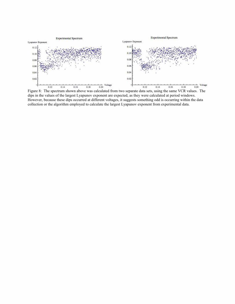
Figure 8: The spectrum shown above was calculated from two separate data sets, using the same VCR values. The dips in the values of the largest Lyapunov exponent are expected, as they were calculated at period windows. However, because these dips occurred at different voltages, it suggests something odd is occurring within the data collection or the algorithm employed to calculate the largest Lyapunov exponent from experimental data.

Phase Space Diagrams from Experimental Data

- 2 0 2 4 6

V

- 4- 2

02

V•

- 2

0

2

4

V••

- 20

24V••

- 2 0 2 4 6

V

- 4

- 2

0

2

V•

Figure 9: Two views of a 3-dimensional phase plot of our electronic circuit. Axes correspond to the x value of the DE and x's derivatives. This data is in the period window around which Lyapunov exponents were calculated from our experimental data, demonstrating good qualitative agreement with our exponents.

- 4- 2

02

V•

- 2 0 2 4 6

V

- 2

0

2

4

V••

- 20

24

V••

- 2 0 2 4 6

V

- 4

- 2

0

2

V•

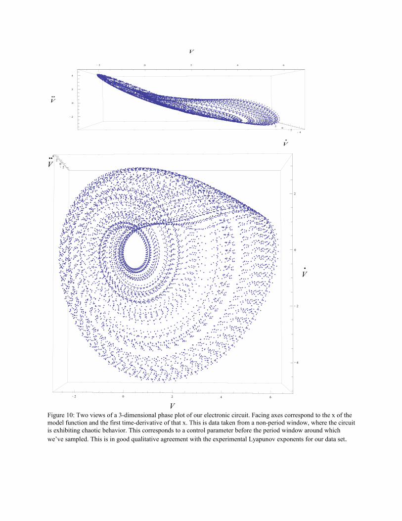
Figure 10: Two views of a 3-dimensional phase plot of our electronic circuit. Facing axes correspond to the x of the model function and the first time-derivative of that x. This is data taken from a non-period window, where the circuit is exhibiting chaotic behavior. This corresponds to a control parameter before the period window around which we’ve sampled. This is in good qualitative agreement with the experimental Lyapunov exponents for our data set.

Bifurcation in Experimental Attractor Data

a) b)

c)

Figure 11: Data collected at lower circuit control voltages, demonstrating apparent bifurcation behavior. (a) is at approximately -4.75V for the control voltage, and is the first bifurcation in the bifurcation series. (b) is at approximately -2V, and is the second bifurcation. (c) is the third bifurcation, at approximately -1.5V. Additional bifurcations are not apparent based on experimental data.

Figure 12: Return maps for two control parameters, one in a chaotic portion of the phase space(upper), with control parameter .5035, and one in a periodic portion of the phase space(lower), with control parameter .5601. Note that the behavior of the return map in these two instances is in very good agreement with the Lyapunov exponent computed for these same control parameters, as well as with our expectations based on the phase plots created at these two control parameter values.

Figure 13: Plots of each eigenvalue as the control parameter changes(x-axis). In blue are the real eigenvalues, and in purple are the imaginary eigenvalues.

Conclusions

Modeling Solutions to the Differential Equation

The models of the differential equation shown above [Figure 6] suggest that the equation can behave both chaotically and periodically. By changing the control parameter, the system displays different behavior and thus is an effective way to change the solutions to the differential equation. It was found that when the control parameter was greater than 0.48, the solution to the differential equation became unpredictable. This phenomenon was also observed in experimental observations. This will be talked about further in the experimental section, but it can be noted that experimental behavior was predicted by the model.

In addition, interesting characteristics of the system could be observed when analyzing the three dimensional phase space diagrams. One particular characteristic was the observation of the fractal surface that the attractor lied upon.

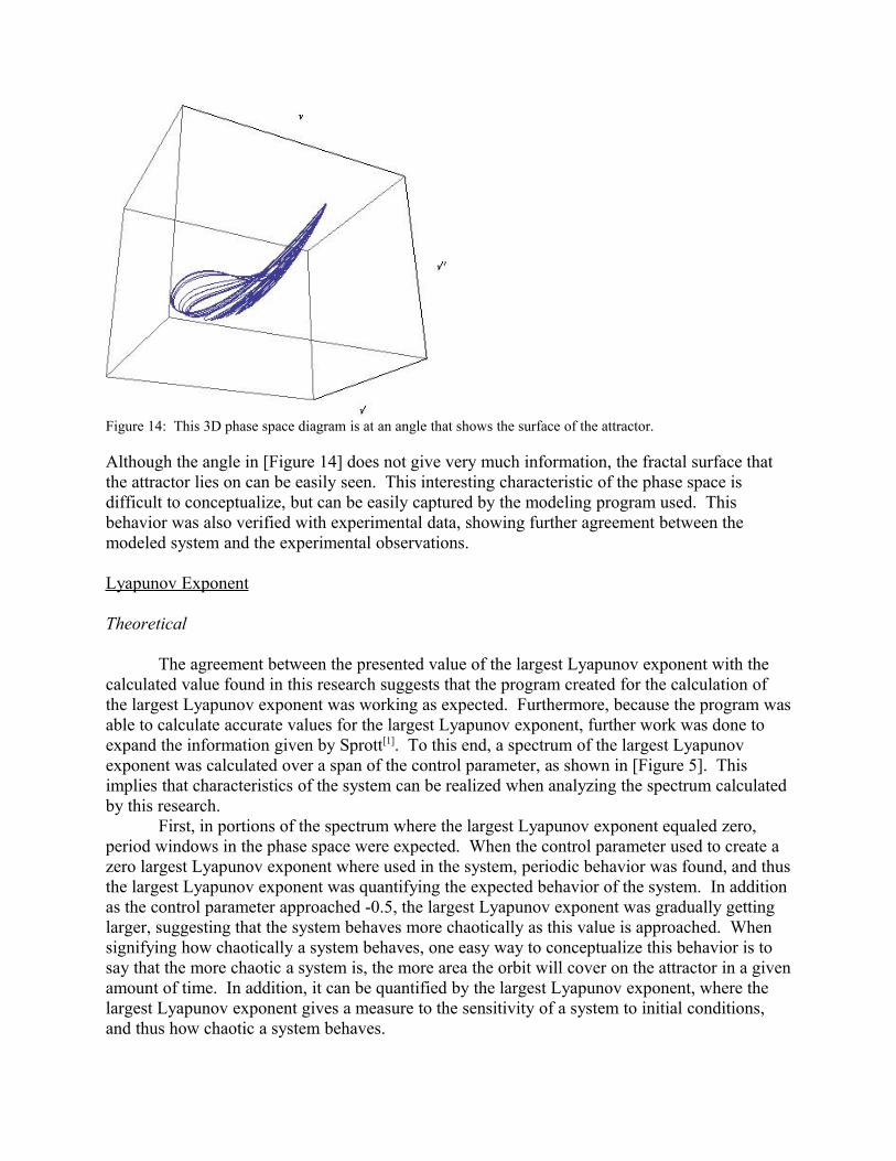
Figure 14: This 3D phase space diagram is at an angle that shows the surface of the attractor.

Although the angle in [Figure 14] does not give very much information, the fractal surface that the attractor lies on can be easily seen. This interesting characteristic of the phase space is difficult to conceptualize, but can be easily captured by the modeling program used. This behavior was also verified with experimental data, showing further agreement between the modeled system and the experimental observations.

Lyapunov Exponent

Theoretical

The agreement between the presented value of the largest Lyapunov exponent with the calculated value found in this research suggests that the program created for the calculation of the largest Lyapunov exponent was working as expected. Furthermore, because the program was able to calculate accurate values for the largest Lyapunov exponent, further work was done to expand the information given by Sprott[1]. To this end, a spectrum of the largest Lyapunov exponent was calculated over a span of the control parameter, as shown in [Figure 5]. This implies that characteristics of the system can be realized when analyzing the spectrum calculated by this research.

First, in portions of the spectrum where the largest Lyapunov exponent equaled zero, period windows in the phase space were expected. When the control parameter used to create a zero largest Lyapunov exponent where used in the system, periodic behavior was found, and thus the largest Lyapunov exponent was quantifying the expected behavior of the system. In addition as the control parameter approached -0.5, the largest Lyapunov exponent was gradually getting larger, suggesting that the system behaves more chaotically as this value is approached. When signifying how chaotically a system behaves, one easy way to conceptualize this behavior is to say that the more chaotic a system is, the more area the orbit will cover on the attractor in a given amount of time. In addition, it can be quantified by the largest Lyapunov exponent, where the largest Lyapunov exponent gives a measure to the sensitivity of a system to initial conditions, and thus how chaotic a system behaves.

Another interesting characteristic that the spectrum provides can be seen when analyzing figures 5 and 6. The arrows labeled A, B and C have different values of the largest Lyapunov exponent caused by only changing the control parameter of the system during the calculation. As can be seen, A has a largest Lyapunov exponent value of zero, B of ~0.7, and C of ~0.9. Thus we would expect that periodic behavior would be observed with a control parameter of 0.5061, and that the system would behavior more chaotically at C then at B. When the phase space diagrams are observed for each of these control parameters, the predicted behavior is realized. At A, the system behaves periodically, and C covers more area of the attractor than B when allowed to run for the same time interval. Thus, it can be concluded that how chaotic a system behaves can be quantified through the largest Lyapunov exponent.

Although there were many successes found with the largest Lyapunov exponent, there were weaknesses in the program that could be improved if further investigations were conducted. First, the program requires nearly a day to calculate one largest Lyapunov exponent. This could be improved by changing the numerical approximation to the solution of the differential equation chosen. Mathematica 6 was used for this purpose in the research, and it was found that the adaptive Runge-Kutta method used for numerical approximations could be overkill for the accuracy needed in the calculations. Furthermore, the program runs for a necessary amount of steps, and then stops after a given amount of iterations have been completed. However, were the program to be modified to exit the calculations upon a given convergence of the largest Lyapunov exponent; it could very well speed up the computation. As the program works now, it takes the same amount of time to calculate a zero value as it does to calculate a positive value. Both of these modifications would greatly improve the programs efficiency and thus make this program an even more powerful tool when analyzing the characteristics of chaotic systems.

Experimental

While collecting the data used to compute the spectrum shown in figure 7, a single period window amid chaotic behavior was observed. Therefore, positive exponent values were expected as well as the sharp valley centered on 0.13 volts. These characteristics of the spectrum are suggestive of the period window directly observed in the experimental data. This indicates that the program is functioning as expected.

In addition, [Figure 8] shows a sharp decrease in the exponent values when voltage is increased, while at the right side of the dips low values of the exponent are intermingled with higher values. Essentially, as the VCR voltage was increasing into the chaotic range, the circuit intermittently switches back and forth between chaotic and periodic behavior before finally resuming steady chaotic behavior. This type of behavior has often been observed on an oscilloscope.

This phenomenon is one explanation for the lack of a zero exponent in the averaged spectrum of [Figure 7]. [Figure 8] also indicates that the voltage at which the period window commenced has a significant uncertainty. Although the uncertainty of the voltage applied by the DAQ board is on the order of hundreds of μV’s, the magnitude of the uncertainty of the circuit's control parameter is almost certainly larger than that of the DAQ's voltage because of the lower precision of the circuit's components, as well as electronic noise present in the equipment which we were using. As well, the shifts in the period window and subsequent lack of an averaged zero exponent may also be the result of some parasitic oscillation which was not completely eliminated through the methods used above.

The presence of positive values of the Lyapunov exponents at the dip indicates that seemingly periodic behavior in the circuit exhibits a net divergence for close neighbors. The only evident difference between periodic behavior in the model and in the circuit is the presence of noise in the circuit.

Computationally introducing pseudo-random values into the differential equation produced no conclusions as to the reason behind the divergence during periodic behavior. In addition, in an ideal random walk, every step made is additively put into memory but that is not the case in our circuit. However, noise pulses do influence the output of the continuous analog calculation and thus perhaps influencing the velocity of a point through phase space. Whether electronic noise is the cause of divergence during periodic behavior of the system is still uncertain however.

Experimental Results

Some interesting features of our experimental system are the “loops” in the attractor. Earlier versions of our attractor [Figure 11] are ellipsoidal in nature, but the attractor at this particular period window is much more twisted, exhibiting a “kink” and a central loop, along with several exterior loops. This behavior is exhibited by both the experimental data[Figure 9, 10], and the model[Figure 6], indicating good overall agreement between the two. The “kink” feature becomes more pronounced after our period window. These two features are common to all the data centered around this period window, even non-periodic data.

These similarities between the model and the system's behavior also indicate that the period window around which our data was taken coincides with the period window predicted to exist between control parameter values of .5075 and .505.

Unfortunately, though a direct relationship between the control parameter of the model and the VCR voltage in the experimental system is expected to exist, determining this relationship in such a way as to translate between VCR voltage and control parameter has proven elusive. We have developed an expression for the effective resistance of the VCR in terms of several different values, including the VCR control voltage. However, when this is combined with our circuit analysis expression for α, we get significantly different control parameter values than what we would expect based on a qualitative comparison of the behavior of the system.

Though the attractor continues to change as we change our control parameter, our electronic system quickly shifts to a section of phase space which our non-ideal components are incapable of emulating. Essentially, the attractor shifts in phase space to a place in which our circuit is saturated. This, coupled with the sensitivity of our DAQ to voltages above 10 Volts, makes it impractical for us to continue investigating this section of the phase space for bifurcation or other interesting behaviors of the circuit.

As for other methods of characterization, we chose to focus extensively on computing Lyapunov exponents to characterize the behavior of the experimental system, as opposed to using any of the other methods applied to the model.

There is some noticeable noise present in our data sets [Figure 9]. This may have the effect of causing some significant variability in the Lyapunov exponents computed for our data. Some of it is due to the sampling uncertainties introduced by our DAQ, and some of it is due to noise which passes through the filters on our power supplies.

Sampling uncertainty is due to the method by which our DAQ collects data. Essentially when the DAQ samples from an analog channel, it collects a voltage, and bins that analog voltage according to a set of voltage ranges representing the minimum resolution of the DAQ. This resolution is variable, according to the voltage measurement range determined by the user at the time of data collection. This has the effect of introducing artifacts due to the DAQs finite resolution. These, however, should be very small, at the 10-4 V level.

The user can choose to sample voltages at finer resolutions than the one used, but the trade-off is that the circuit must then be scaled such that its output voltages are within this new, smaller range. Any voltage values outside the sample range are clipped to within the maximum or minimum voltage of the sample range.

This requirement to adjust the sample range arises because the only way to control the DAQs voltage resolution is to reduce the size of the sample range. This adjustment would have the overall effect of increasing precision while bringing the collected voltages closer to the noise floor inherent in any analog electronic system. Essentially, the two extremes are: noisy, precise data, or clean, imprecise data. We sought, in our choice of measurement range, a compromise between these two extremes.

Accounting of Funds

Parts, including resistors, ICs, and capacitors: 230.18National Instruments 6251 M-Series Data

Acquisition Board(USB)1261.72

The CWU SPS would like to thank the SPS National Office for their generous grant.

References

1. J.C., Sprott, “Chaos and Time Series Analysis,” Oxford University Press, 22-123 (2003).

2. J. C. Sprott, “Simple chaotic systems and circuits,” Am. J. Phys. 68 (8), 758-763 (August

2000).

3. Horowitz, Paul, Hill, Winfield, “The Art of Electronics” 2nd Ed, Cambridge University

Press, 222 (1980).

4. Texas Instruments, “µA741 General-Purpose Operational Amplifiers,” (2000).

<http://www.us.oup.com/us/pdf/microcircuits/students/amps/ua741-ti.pdf>

5. Kiers, Ken, Schmidt, Dory, Sprott, Julien C., “Precision measurements of a simple

chaotic circuit,” Am. J. Phys. 72 (4), 503-508 (April, 2004).

6. Analog Devices. “AD734 10MHz, 4-Quadrant Multiplier/Divider,” (1999).

<http://www.analog.com/UploadedFiles/Data_Sheets/AD734.pdf>

7. National Semiconductor, “LM13700 Dual Operational Transconductance Amplifiers with

Linearizing Diodes and Buffers,” (2004).

<http://cache.national.com/ds/LM/LM13700.pdf>

8. Kuhn, Kenneth A., “Practical Application of Op-Amps,”

<http://www.kennethkuhn.com/students/ee431/text/op_amp_practical_applications.pdf>

(2002).

9. Ruskeepaa, H., “Mathematica Navigator Second Edition,” Elseveir Science &

Technology. (2003)

10. Karu, Zohar Z., “Signals and Systems Made Ridculously Simple,” ZiZi Press (1995).

11. J. C. Sprott, “Some simple chaotic jerk functions,” Am. J. Phys. 65 (6), 537-543 (June,

1997).

12. National Instruments, “NI 625x Specifications,” 2007.

<http://digital.ni.com/manuals.nsf/websearch/210C73CBF91128B9862572FF0076BE85

>

13. Rosenstein, Michael T., Collins, James J., De Luca, Carlo J., “A Practical method for

calculating largest lyapunov exponents from small data sets,” Physica D 65 (1-2), (May

1993).