Chaotic Dynamics in Credit ConstrainedEmerging Economies∗

Jordi CaballéUnitat de Fonaments de l’Anàlisi Economica and CODE

Universitat Autònoma de Barcelona

Xavier JarqueDepartament de MatematiquesUniversitat de Barcelona

Elisabetta MichettiDipartimento di Istituzioni Economiche e Finanziarie

Università degli Studi di Macerata

March 16, 2004

Abstract

This paper analyzes the role of financial development as a source of en-dogenous instability in small open economies. By assuming that firmsface credit constraints, our model displays a complex dynamic behav-ior for intermediate values of the parameter representing the level offinancial development of the economy. The basic implication of ourmodel is that economies experiencing a process of financial develop-ment are more unstable than both very underdeveloped and very de-veloped economies. Our instability concept means that small shockshave a persistent effect on the long run behavior of the model andalso that economies can exhibit cycles with a very high period or evenchaotic dynamic patterns.

JEL classification codes: O16, C62.

Keywords: Chaotic Dynamics, Credit Constraints, Financial De-velopment.

∗Financial support from the Spanish Ministry of Science and Technology throughgrants SEC2003-306, and HI2001-0039; and from the Generalitat of Catalonia throughthe Barcelona Economics program of CREA and grants SGR2001-00162, SGR2001-00173,and BFM2002—01344 is gratefully acknowledged.

Correspondence address: Jordi Caballé. Universitat Autònoma de Barcelona. Departa-ment d’Economia i d’Història Econòmica. Edifici B. 08193 Bellaterra (Barcelona). Spain.Phone: (34)-935.812.367. Fax: (34)-935.812.012. E-mail: Jordi.Caballe@uab.es

1 Introduction

This paper considers a model where the process of financial developmentcould be a source of endogenous instability for small open economies.Our basic macroeconomic model describes a dynamic open economy wherefirms face credit constraints. This means that the maximum amountentrepreneurs can borrow is proportional to the amount of their currentlevel of wealth.

Several authors have discussed the implications of borrowing constraintson the persistence of business cycles (Bernanke and Gertler, 1989) and onthe emergence of cycles in closed economies (Azariadis and Smith, 1998;and Kyotaki and Moore, 1997). Moreover, Aghion et al. (2000) showedthat, when firms are credit constrained and there is debt issued both indomestic and in foreign currency, currency crises could easily arise. Later on,Aghion et al. (2001) constructed a simple monetary model where currencycrises are driven by the interplay between the credit constraints of domesticfirms and the existence of nominal price rigidities, which in turn leads tomultiple equilibria. We will use a similar formulation, although we willfocus on the real side of the economy like in Aghion et al. (1999) andAghion et al. (2003). In particular, Aghion et al. (1999) developed asimple macroeconomic model where the combination between capital marketimperfections (taking the form of borrowing constraints due to moral hazardproblems) and unequal access to investment opportunities across individuals(due to the physical separation between savers and investors) generatesendogenous and permanent fluctuations in aggregate GDP, investment,and interest rates. In their paper the endogenous cycles arise from twodistinct factors. A larger amount invested generates more profits and moreinvestment. However, a large investment pushes interest rates up and thisreduces future profits and, thus, future investment. Finally, Aghion et al.(2003) consider a model close to ours to conclude that, at an intermediatelevel of financial development, economies could present unstable dynamics,while either underdeveloped or very developed ones are stable. They showthat the fixed point of the entrepreneurs’ wealth is stable when the level offinancial development is either “high” or “low”, while for some intermediatevalues of financial development the attractor is a two stable cycle. However,it does not follow from their work the existence of high period cycles or ofchaotic dynamics.

Using bifurcation analysis we will show that economies with either verydeveloped or very undeveloped financial markets are structurally stable,while emerging markets (with intermediate levels of financial development)are unstable in the sense that they could exhibit chaotic dynamics and,thus, the evolution of the endogenous variables of the model turns out tobe unpredictable. Therefore, when the economy is going through a phase offinancial development, the dynamics of the economic system could change

1

dramatically and evolve from a stable fixed point to a stable cycle and,finally, to an attractor displaying aperiodic dynamic behavior.

The fluctuations displayed by the model we consider are due to twoforces. First, larger investment raises both output and profits. Larger profitsimprove creditworthiness and raise borrowing, which in turn leads to a largeramount of investment. Simultaneously, this increase leads to a rise in thedemand for the country specific input (which has constant supply) and, thus,in its relative price. This rise in input prices leads to lower profits and reducecreditworthiness, borrowing and investment, which in turn makes aggregateoutput fall. The conclusion is that financial development could destabilizeeconomies exhibiting an intermediate level of financial development, whichagrees with the experience documented for a number of countries.1

Other authors have investigated the possibility of chaotic dynamics inmacroeconomic models by using the classical paper by Li and Yorke (1975).Thus, Stutzer (1980) and Day (1983) showed the possibility of obtainingaperiodic paths in simple models of population growth. Benhabib and Day(1981) investigated how preferences depending on past experience could leadto erratic behavior. The same authors (Benhabib and Day, 1982) have alsocontributed to this literature by characterizing the conditions under whichchaos is obtained in overlapping generation models. Finally, Deneckere andPelikan (1986) and Boldrin and Montrucchio (1986) analyzed the possibilityof chaotic paths in neoclassical multi-sector models. Our model adds to thisliterature a very simple model with an imperfection in the financial market,which is a source of very complex dynamics for a wide range of parametervalues.

The paper is organized as follows. In Section 2 we present the model. InSection 3 we perform the dynamic analysis in order to assess the plausibilityof chaotic dynamics when entrepreneurs do not receive any exogenousincome. In this case we present some general properties of the attractors ofthe dynamic system depending on the parameter values of the model. InSection 4 we extend the analysis to the general case with positive exogenousincome and we show the global stability of either very developed or veryunderdeveloped financial markets. Section 5 concludes our paper. AppendixA contains some definitions concerning periodic and chaotic dynamics, whileAppendix B contains the proofs of all the results of the paper.

2 The Model

Let us consider a small open economy in discrete time. There are two typesof individuals in this economy: the borrowers (or entrepreneurs), who owna production technology and may invest either in the production activity

1See, among many others, De Melo et al. (1985), Galvez and Tybout (1985), and Petreiand Tybout (1985).

2

or in the international capital market, and the lenders (or families), whocannot directly invest in the production activity, but they can either lendfunds to the entrepreneurs or invest in the international capital market. Theinternational gross rate of interest is constant and equal to r > 0 .

This economy produces a unique tradeable good. The productionfunction of this good uses capital and a country specific input (like land, realestate, or a non-tradeable natural resource), which has a constant supplyequal to Z. Moreover, the tradeable good can be consumed or accumulatedas productive capital for the following period’s production. The outputyt of the tradeable good in each period is obtained through the followingCobb—Douglas production function:

yt = F (Kt, zt) = A(Kρt z

1−ρt ), with ρ ∈ (0, 1), (1)

where zt is the amount of the country specific input used in period t, Kt isthe amount of capital, and A is the total factor productivity. We assumethat A > r , since the entrepreneurs would do not find profitable to invest inthe production activity otherwise. We assume that capital fully depreciatesafter one period.

The total investment It in period t is devoted to purchase both capitaland country specific input. For a given level of investment, the optimaldemand zt for the country specific input in each period t arises from themaximization of the profit function subject to the budget constraint

It = Kt + ptzt,

where pt is the price of the country specific input expressed in units of thetradeable good. The first order condition of the previous problem yields

zt =

µ1− ρ

pt

¶It. (2)

Therefore, the country specific input equilibrium price is obtained byequating the country specific input equilibrium demand (2) with its constantsupply Z,

pt =

µ1− ρ

Z

¶It. (3)

Finally, substituting (2) into (1), we may write the total equilibrium outputyt in terms of the level of investment It and the price pt,

yt = G(pt)It, with G(pt) =Aρρ(1− ρ)1−ρ

p1−ρt

. (4)

Note that G(pt) can be viewed as the gross return of a unit of investment.

3

We assume that the credit market operates imperfectly due to, say, eitheradverse selection or moral hazard considerations. In particular, we assumethat an entrepreneur with wealth Wt may borrow at most the amount Lt,with Lt ≤ µWt, as the entrepreneur’s wealth serves as a collateral forthe loan.2 Therefore, the investment in each period is bounded aboveby (1 + µ)Wt. The proportional coefficient µ ≥ 0 can be viewed as acredit multiplier reflecting the level of financial development of the domesticeconomy.

The dynamics of the model is described as follows. In period tentrepreneurs decide the amount of borrowing (and, thus, of investment),and pay the cost of the country specific input. Hence, at period t + 1 theentrepreneurs receive the corresponding profits and pay the cost of debt rLt.We assume here that entrepreneurs save a constant fraction (1−α) of theirtotal wealth at the end of each period, where α is the constant propensityto consume.3 Therefore, the dynamics of the entrepreneurs’ wealth is givenby

Wt+1 = (1− α) (e+ yt − rLt) , (5)

where e ≥ 0 is an exogenous income in terms of tradeable good andLt ≤ µWt.

Let us consider first the case where G(pt) ≥ r, which means that theproductive investment return exceeds the international capital market returnand, hence, the entrepreneurs will invest in the productive project the largestamount they can borrow,

It = (1 + µ)Wt. (6)

Total output is now given by

yt = G(pt)(1 + µ)Wt.

Substituting (3) and (6) in the previous equation, we obtain the total outputin period t as a function of wealth,

yt = ξW ρt , with ξ = Aρρ(1 + µ)ρZ1−ρ. (7)

As follows from (5), the dynamics of entrepreneurs’ wealth is

Wt+1 = (1− α) (e+ yt − rµWt) , (8)

which, after using (7) becomes

Wt+1 = (1− α)W ρ¡ξ − rµW 1−ρ¢+ (1− α)e. (9)

2This is the type of constraint found in Bernanke and Gertler (1989).3This simple saving rule could be derived under the assumption that entrepreneurs

maximize the discounted sum of instantaneous utilities when these utilities are logarithmic(see Woodford, 2003).

4

The previous equation describes the dynamics of the entrepreneurs’ wealthas long as

G(pt) ≥ r.

Combining (3), (4), and (6), the previous inequality holds wheneverW ≤Wm , where the critical point Wm is given by

Wm =

µA

r

¶ 11−ρ

µZ

1 + µ

¶ρ

ρ1−ρ . (10)

As it can be immediately seen from (9), the impact of a change in thevolume of current wealth could be ambiguous. This is so because, even ifan increase in wealth raises the investment, the amount of invested wealthdepends negatively on the price p of the country specific input, and this pricedepends positively on current wealth. Hence, two distinct effects coexist: apositive wealth effect on investment for a given price p and a negative priceeffect via a greater demand for the country specific input.

Let us now consider the case where G(pt) < r . In this case theentrepreneurs have no incentives to borrow up to the credit constraintbecause the return from the productive investment is lower than the returnfrom the international capital market. Hence, they borrow until the pointwhere the productive investment return is equal to the international capitalmarket return, that is, until yt − rLt = rWt. Therefore, substituting theprevious equation into (5), we find the dynamic equation for the wealthwhen W > Wm ,

Wt+1 = (1− α) (e+ rWt) . (11)

The asymptotic behavior of wealth is thus determined by the iterates ofthe following function (see (9) and (11)):

f(Wt) =

⎧⎪⎨⎪⎩(1− α)

he+W ρ

t (ξ − rµW 1−ρt )

i≡ f l(Wt), if 0 ≤Wt ≤Wm,

(1− α) (e+ rWt) ≡ fr(Wt), if Wt > Wm.

(12)

The iterates of f describe a one-dimensional discrete dynamical system.In the next sections we will analyze the general dynamic properties of thesystem depending on the parameters of the model and we will determinethe cases where complex (or even chaotic) dynamics could appear. Notethat the dynamic behavior of the other endogenous variables of the model,output yt, investment It, and price of the country specific input pt, isentirely determined by the behavior of the entrepreneurs’ wealth, as followsimmediately from the previous analysis.

5

It is straightforward to see that, for any value of the parameters, f l(Wt)is a single peaked function with a maximum at

WM =

µrµ

ξρ

¶ 1ρ−1

, (13)

while fr(Wt) is linear. We notice, however, that f(Wt) has a local maximumat WM only if WM < Wm.

3 Dynamical Analysis Without Exogenous Income

In this section we describe the long run dynamics of the model when theexogenous income e is equal to zero. This analysis will be helpful in the nextsection, where we study the case with positive exogenous income, e > 0.For the rest of the paper we will assume the empirically plausible inequality(1− α)r < 1 , which ensures the existence a positive fixed point for thefunction f.

When e = 0 it is immediate to see that f has a repelling fixed point atW = 0. Other dynamic properties are summarized in the following lemma:

Lemma 3.1. (a) If µ ∈h0, ρ

1−ρ´, then WM > Wm and f is a strictly

increasing function. Moreover f has a unique positive, globally stablefixed point W ? ∈ (0,Wm) .

(b) If µ ∈h

ρ1−ρ ,

ρr(1−α)(1−ρ)

´, then WM ≤Wm and f has a unique

positive, globally stable fixed point W ? ∈ ¡0,WM¢.

(c) If µ ∈h

ρ(1−α)r(1−ρ) ,∞

´, then f has a unique positive fixed point

W ? ∈ £WM ,Wm¢and f 0(W ?) ≤ 0 .

From the previous lemma we conclude that, in order to obtain a chaoticdynamics for the entrepreneurs’ wealth, the parameter value of µ must besufficiently high. In particular, we must have µ ≥ ρ

(1−α)r(1−ρ) . Moreover,the previous lemma states the global stability for economies with low valuesof µ, that is, for economies exhibiting a low level of financial development.As we will see in Section 4, this result also holds in the case of positiveexogenous income.

Next we study the first period bifurcation of our model.

Lemma 3.2.

(a) If µ ∈h

ρr(1−α)(1−ρ) ,

1+ρr(1−α)(1−ρ)

´, then the fixed point W ? is the unique

positive globally stable fixed point of f .

6

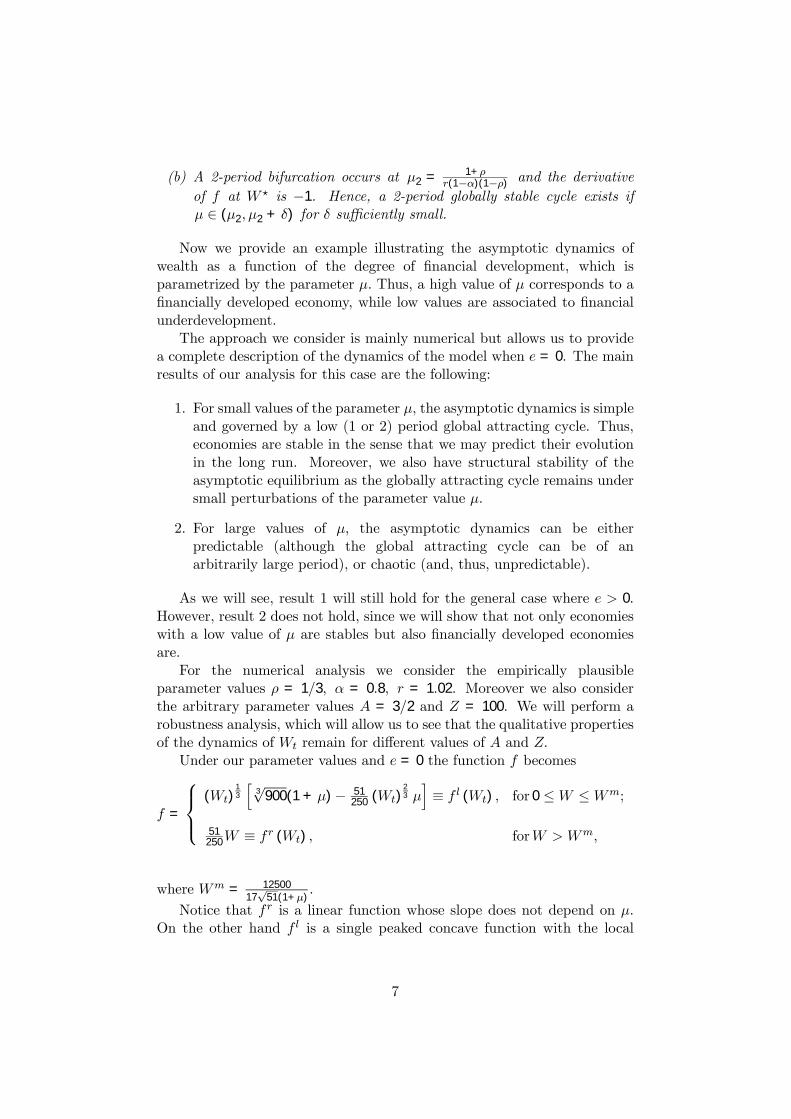
(b) A 2-period bifurcation occurs at µ2 = 1+ρr(1−α)(1−ρ) and the derivative

of f at W ? is −1. Hence, a 2-period globally stable cycle exists ifµ ∈ (µ2, µ2 + δ) for δ sufficiently small.

Now we provide an example illustrating the asymptotic dynamics ofwealth as a function of the degree of financial development, which isparametrized by the parameter µ. Thus, a high value of µ corresponds to afinancially developed economy, while low values are associated to financialunderdevelopment.

The approach we consider is mainly numerical but allows us to providea complete description of the dynamics of the model when e = 0. The mainresults of our analysis for this case are the following:

1. For small values of the parameter µ, the asymptotic dynamics is simpleand governed by a low (1 or 2) period global attracting cycle. Thus,economies are stable in the sense that we may predict their evolutionin the long run. Moreover, we also have structural stability of theasymptotic equilibrium as the globally attracting cycle remains undersmall perturbations of the parameter value µ.

2. For large values of µ, the asymptotic dynamics can be eitherpredictable (although the global attracting cycle can be of anarbitrarily large period), or chaotic (and, thus, unpredictable).

As we will see, result 1 will still hold for the general case where e > 0.However, result 2 does not hold, since we will show that not only economieswith a low value of µ are stables but also financially developed economiesare.

For the numerical analysis we consider the empirically plausibleparameter values ρ = 1/3, α = 0.8, r = 1.02. Moreover we also considerthe arbitrary parameter values A = 3/2 and Z = 100. We will perform arobustness analysis, which will allow us to see that the qualitative propertiesof the dynamics of Wt remain for different values of A and Z.

Under our parameter values and e = 0 the function f becomes

f =

⎧⎪⎨⎪⎩(Wt)

13

h3√

900(1 + µ)− 51250 (Wt)

23 µi≡ f l (Wt) , for 0 ≤W ≤Wm;

51250W ≡ f r (Wt) , forW > Wm,

where Wm = 1250017√

51(1+µ).

Notice that f r is a linear function whose slope does not depend on µ.On the other hand f l is a single peaked concave function with the local

7

maximum at the point

WM =12500(1 + µ)1/2

153√

17µ3/2.

The asymptotic dynamics described by f has to be studied depending on therelative position ofWm, f(Wm),WM and f(WM). We will first perform ouranalysis for relatively small values of µ (for which the dynamics is simple)and then we consider relatively large values of µ (for which the dynamicsbecomes complex).

For positive values of µ smaller than 2.451, the dynamics of f is trivial,since the stable steady state of wealth belongs to the interval where f l

is increasing. Moreover, for µ ∈ (0, 0.5] the steady state W ∗ lies in theinterval (0,Wm] , whereas W ∗ ∈ ¡0,WM

¤for µ ∈ (0.5, 2.451] . Therefore,

the path of wealth is globally stable and monotonic around the steady stateW ∗ (see Panel (a) of Figure 1). For values of µ larger than 2.451, theattracting fixed point W ? belongs always to the decreasing part of f l andf 0(W ?) = 1

3 − 17µ125 . Therefore, for µ ∈ (2.451, 9.804), the path of Wt is

globally stable and the convergence is oscillating around the steady state(see Panel (b) of Figure 1). When µ = 9.804 we obtain the first perioddoubling bifurcation and the resulting attracting cycle has period 2 andbelongs to the interval (WM , f(WM)). The pair

¡W 1,W 2

¢gives the two

points of the 2-period cycle. Notice that when µ ∈ (9.804, 11.203) it holdsthat WM < W 1 < W 2 < Wm (see Panel (c) of Figure 1). At µ = 11.203we have f(WM) = Wm, so that when µ ∈ (11.203, 25.239) the attracting2-period cycle

¡W 1,W 2

¢lies in the invariant set (WM , f(WM)) and satisfies

WM < W 1 < Wm < W 2 as f(Wm) < WM and f(WM) > Wm for thosevalues of µ (see Panel (d) of Figure 1).

[Insert Figure 1]

The previous analysis shows that the interval µ ∈ [0, 25.239) gives raiseto simple dynamics, where the entrepreneurs’ wealth is asymptotically givenby a stable fixed point or a 2-period stable cycle. Therefore, in this casewe are facing a predictable and structurally stable economy in the long run.In fact, the dynamics of wealth for those values of the parameter µ agreeswith our Lemmae 3.1 and 3.2, since ρ

1+ρ = 0.5, ρr(1−α)(1−ρ) = 2.451, and

1+ρr(1−α)(1−ρ) = 9.804. As we will show in Section 4, this simple dynamics stillholds when e > 0.

A more complex dynamics appears when µ increases above the value25.239. When µ = 25.239 we get f(Wm) = WM and Wm < f(WM) . Asthe value of µ increases, the asymptotic dynamics belongs to the interval[f(Wm), f2(Wm)]. Moreover, at the value µ = 25.239, there is an attracting2-period cycle with WM < W 1 < Wm < W 2 < f2(Wm).

8

In order to study the case of those more financially developed economiesin a simpler manner, we first compose the function

f : [f(Wm), f2(Wm)]→ [Wm, f2(Wm)]

with an homeomorphism h so that g = h(f(h−1)) is a function from [0, 1]to [0, 1].4 Obviously, the dynamics associated with f and g display the samequalitative properties. The advantage of working with the function g insteadof f lies on the fact that the windows where the asymptotic dynamics occursis [0, 1], which is independent of µ. Therefore, the analysis of the comparativestatics for the different values of µ becomes much easier. Note that whenµ > 25.239 the continuous function g maps the interval [0, 1] into itself andthe steady state is unstable, as follows from Lemma 3.2. Therefore, wealthnever grows without bound nor converges to a steady state (for almost allinitial conditions). Hence, it must fluctuate forever, either converging to acycle or following an aperiodic path (see Definition 6 in Appendix A). Wenext investigate under which circumstances the attracting set [0, 1] containsattracting high-period cycles or becomes a chaotic attractor.

If gl and gr denote the two components of g corresponding to f l and f r,respectively, we get after some computations that

gl(Wt) =δµWt − 25µ

¡510 + 51(−10 + 3

√204)Wt

¢− 62500 + 1250 3

q102

¡250 + βµWt

¢(1 + µ)

250βµ,

gr(Wt) =−49750

250βµ+ 0.204Wt,

Wm =49750

51βµ, with

βµ = −250 + 253√

204 + (−51 + 253√

204)µ and

δµ = −51³−51 + 25

3√

204´µ2.

Note that gr is a linear function with a constant slope, gl is a monotonedecreasing function and Wm → 0 as µ → ∞. We plot the function g inFigure 2.

[Insert Figure 2]

In what follows we will show that, as we increase the value of theparameter µ, dynamic complexity will arise. Recall that the multiplier %of a n-period cycle is

% =nYi=1

f 0(W i),

4The function h is simply a linear transformation depending on µ that assigns the value0 to f(Wm) and the value 1 to f2(Wm) for each µ.

9

where©W iªni=1

are the points of the n-period cycle. It can be seen fromthe function g that the attracting 2-period cycle (W 1,W 2) obtained atµ = 25.239 remains for a while until we arrive at the new period doublingbifurcation. Panel (a) of Figure 3 displays the 2-period cycle for µ = 28. Thedoubling bifurcation occurs when the multiplier % of the 2-period attractingcycle is -1, that is, when µ = 48.055. After this bifurcation the asymptoticdynamics is given by an attracting 4-period cycle with positive multiplierand two points lying in the interval (0,Wm) and two points lying in theinterval (Wm, 1). Panel (b) of Figure 3 displays a 4-period cycle for µ = 50 .

[Insert Figure 3]

At µ = 53.953 one of the points of the 4-period cycle is the criticalpoint Wm. The presence of the non-differentiable point Wm makes thisbifurcation atypical (it is called a “border collision bifurcation”). However,applying Corollary 3 in Nusse and Yorke (1995), it can be proved that abifurcation from a 4-period cycle to a 8-period cycle occurs at this value ofµ.

When µ = 54.925 the critical point Wm of the function f is preperiodic(see Definition 5 in Appendix A) as f(Wm) = 0, f(0) = 1, and f(1) =W ?.5 Thus, for this value of µ, no attracting cycles exist, since the basinof attraction of these cycles cannot contain the critical point Wm (seeProposition 2 in Nusse and Yorke, 1995). Consequently, the set of aperiodicpaths under the map g has full Lebesgue measure in [0, 1], which means thatthe interval [0, 1] is a chaotic attractor under g (see Definition 9 in AppendixA).6 Note that the fact that the interval [0, 1] is a chaotic attractor underg implies immediately that the chaotic attractor under the original map fhas positive Lebesgue measure when µ = 54.925.

Finally, when µ = 60.936 the image ofW = 1 is equal toWm and, hence,we obtain a 3-period cycle. This parameter value is the initial point of aninterval for which an attracting 3-period cycle exists (see the Panel (a) ofthe bifurcation diagram shown in Figure 4).

[Insert Figure 4]

The existence of two distinct values of µ, one giving raise to chaoticdynamics and the other generating simple stable dynamics repeats over andover as µ increases, as the following proposition confirms:

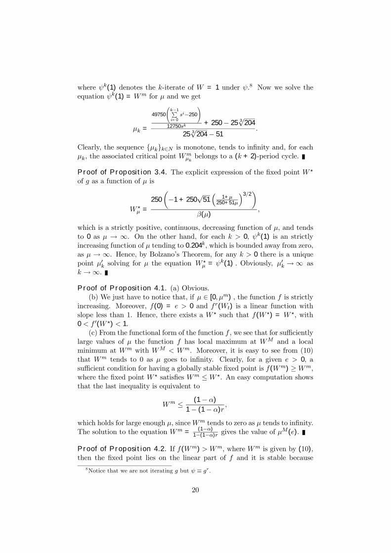
Proposition 3.3. For any integer k > 0, there exist a value µk of theparameter µ such that the corresponding critical point Wm

µkof the function

5A preperiodic point is usually called a Misiurewicz point.6Moreover, the topological entropy of the map f for µ = 54.925 is positive, which

confirms the existence of a chaotic attractor (see Corollary 4.4.9 in Alsedà et al., 2001).Recall that the topological entropy is given by lim

n→∞lnNnn

where Nn is the number of

distinct n-period cycles.

10

f is a (k + 2)−periodic point. Moreover the sequence {µk} is monotonicallyincreasing in k and µk →∞ as k →∞.

The next proposition shows the existence of a special preperiodic pointleading at a (k + 2)−period cycle for all k > 0.

Proposition 3.4. For any integer k > 0, there exist a value µ0k of theparameter µ such that the critical point Wm

µ0kof the function f is preperiodic

and its preperiod is k + 2. Moreover the sequence {µ0k} is monotonicallyincreasing in k and µ0k →∞ as k →∞.

In our example, the first values of the two sequences {µk} and {µ0k} areµ1 = 60.936, µ2 = 304.676, µ3 = 1499.48, µ4 = 7356.363,

µ01 = 54.925, µ02 = 298.793, µ03 = 1493.594, µ04 = 7350.175.

We show in Figure 4 the bifurcation diagrams as µ increases. Thenumerical experiments illustrate our previous statements. First, we observelarge intervals for the values of µ where the dynamics only bifurcates fromstable cycles of period k to stable cycles of period of period 2k. In theseintervals the economy is predictable and structurally stable. Second, weobserve values of µ where the dynamics is extremely complex and theeconomy is unpredictable. Third, based on the previous two propositions,this pattern repeats over and over as µ increases and, hence, there is not avalue of µ above which stability holds in the long run. As we will prove inthe following section, this last result does not longer hold for the case e > 0.

Recall that the parameters values we have been using for the totalfactor productivity A and for the supply of the country specific input Zare arbitrary. Here we want to show by means of numerical simulationsthat they do not affect the qualitative dynamics of the model but only thequantitative ones. In Figures 5(a) and 5(b), we present the bifurcationdiagrams when A = 20 or Z = 300, respectively. In these simulations we areusing the original function f because it allow us to show that the dynamicsis quantitatively different, since the amplitude of the invariant set where theasymptotic dynamics lies is changing. Moreover, we can observe that thequalitative dynamics remains unchanged: we have the same bifurcations atthe same values of µ we presented in Figure 4 and, thus, all the previousresults still hold. This fact is confirmed if we look at Figures 6(a) and 6(b),where we can see how the dynamics change when both the parameters µand A or µ and Z change. We assign a different shading to each region inthe (A,µ) and (Z, µ) planes, according to the type of attractor of the mapf . The different regions are separated by straight horizontal lines, whichmeans that the choice of the values for A or Z does not affect qualitativelythe asymptotic dynamics of the model.

[Insert Figures 5 and 6]

11

4 Dynamic Analysis with Positive ExogenousIncome.

Let us now study the dynamics of the model in the case with positiveexogenous income, that is, when e > 0. The resulting dynamics is nowdetermined by the function (12). Obviously, the values of the critical pointWm and of the maximum WM are the same as when e = 0 (see (10) and(13)). Panel (a) of Figure 7 illustrates the changes of the function f as eincreases. However, both the existence and the qualitative properties of theattracting sets are affected by the fact that e > 0. Although for this caseit is not longer possible to obtain explicit expressions neither for the fixedpoint nor for its derivatives, we may use the computations of Section 3 toshow the existence and uniqueness of global attractors in this new setting.

[Insert Figure 7]

The main result of this section is that, for any positive exogenous incomee, we have stable dynamics for Wt (that is, a globally stable fixed point) forlow as well as for high levels of financial development. Moreover, for anypositive e, there are intermediate levels of financial development (that is, abounded interval of values of µ) for which the dynamics would be complexor even chaotic.

Proposition 4.1. Let e > 0.

(a) W = 0 is not a fixed point.

(b) The function f(Wt) has a unique positive, globally stable fixed pointW ? for each µ ∈ [0, µm) , where µm ≡ ρ

(1−ρ) .

(c) The function f(Wt) has a globally stable fixed point W ? withW ? ≥Wm for each µ ∈ £µM(e),∞¢ , where

µM(e) ≡µA

r

¶ 11−ρ

Zρρ

1−ρ 1− (1− α)r

(1− α)e− 1 .

The previous proposition shows that, for each positive value of e, thereexists a large enough value µM(e) of the parameter µ guaranteeing thestability of financially developed economies. Intuitively, this is due to thefact that as µ→∞ the critical point Wm tends to (1 − α)e. The latterlimit point is positive so that it has to pass from the right to the left ofthe 45◦-degree line of the Panel (b) in Figure 7. Therefore, the stabilityof financially developed economies is obtained if and only if e is positive.

12

Note in this respect that global stability does not hold for e = 0 as wasestablished in Lemma 3.3.

Panel (a) of Figure 8 shows the bifurcation diagram for the parametervalues of our benchmark economy with e = 4 . Moreover, we shouldemphasize that µM(e) is a decreasing function of e, as is shown in Panel(b) of Figure 8. The global picture is thus as follows. Let us fix e and,then, for small values of µ (µ < µm) we have a globally stable fixed pointlying below Wm and, for high values of µ (i.e., when µ ≥ µM(e)) we havealso a globally stable fixed point lying above Wm. For intermediate valuesof financial development we may found complex or even chaotic dynamics.As follows from Propositions 3.3 and 3.4, the potential dynamic complexitydepends on how many terms of the sequences {µk} or {µ0k} are smaller thanµM(e). In particular, for high values of e the value of µM(e) is so small thatthe attracting set is given by either a fixed point or a low period cycle, whilefor small values of e the value of µM(e) is large enough so that emergingeconomies admit chaotic behavior.

[Insert Figure 8]

To understand the resulting dynamics of our model note that, on theone hand, for low values of µ the credit constraint faced by entrepreneursis so strong that investment is insensitive to the amount of current wealth.On the other hand, for very high values of µ the amount of current wealth isalso irrelevant for investment since entrepreneurs are not credit constrained.Only for intermediate values of the parameter representing the degree offinancial development, the current level of investible funds are relevant forthe determination of investment and, thus, for future wealth.

Note that in the chaotic region the path of the entrepreneur’s wealthis sensitive to the initial conditions, as is implied by the aperiodicity ofthe dynamics. Therefore, small transitory shocks end up having permanenteffects in the long run.

While Proposition 4.1 establishes the maximum value of µ such that theeconomy is stable for each choice of e > 0, the following proposition definesa minimum value of e such that the economy is stable for every µ ≥ 0.

Proposition 4.2. Let µ ≥ 0. The function f(Wt) has a globally stable fixedpoint W ? for each e > e?, where

e? ≡ 1− (1− α)r

1− α

µA

r

¶ 11−ρ

Zρρ

1−ρ .

The previous proposition shows that the greater is the exogenous income,the more likely is that the economy be stable.

13

5 Conclusions

We have studied the asymptotic dynamics of entrepreneurs’ wealth in a smallopen economy with credit constrains under a Cobb-Douglas technology. Asimilar model has been considered in Aghion et al. (2003) using a Leontiefftechnology. These authors only showed that financial underdeveloped, aswell as very developed economies, present stable fixed points, whereasintermediate levels of financial development could be a source of instability.They obtain the instability result by showing that, for some range ofparameter values, a 2-period cycle appears.

Our analysis differs from that of Aghion et al. (2003) in the followingaspects:

• We show that financially developed economies present complexdynamics when there is no exogenous income of the tradeable good.However, very developed economies are stable when entrepreneurshave positive exogenous income;

• We derive sufficient conditions on the parameter values of the modelin order to obtain global stability;

• We show that economies with an intermediate level of financialdevelopment could present dynamics more complex than a 2-periodcycle, since they could display cycles with a high period or even chaoticdynamics. Those cycles are robust as they remain under perturbationsof the parameter µ representing the level of financial development.In this case, even though the dynamics becomes complex, it is stillpredictable. This predictability does not longer hold in the chaoticregion. Moreover, when the economy displays chaotic dynamics, smalltemporary shocks turn out to have permanent effects.

Note that when there is no exogenous income, the complex dynamicsoccurs for arbitrarily large values of the parameter µ. However, the rangeof values of µ for which complexity arises is bounded when the exogenousincome is positive. Thus, in such a case, there is a sufficiently high level offinancial development that guarantees stability in the long run.

14

References

[1] Alsedà, L., J. Llibre and M. Misiurewicz (2001), CombinatorialDynamics and Entropy in Dimension One, World Scientific. Singapore.

[2] Aghion, P., P. Bacchetta, and A. Banerjee (2000), A Simple Model ofMonetary Policy and Currency Crises, European Economic Review 44,728—738.

[3] Aghion, P., P. Bacchetta, and A. Banerjee (2001), Currency Crises andMonetary Policy in an Economy with Credit Constraints, EuropeanEconomic Review 45, 1121—1150.

[4] Aghion, P., P. Bacchetta, and A. Banerjee (2003), FinancialDevelopment and the Instability of Open Economies, Journal ofMonetary Economics (forthcoming).

[5] Aghion, P., A. Banerjee, and T. Piketty (1999), Dualism andMacroeconomic Volatility, Quarterly Journal of Economics 114, 1357—1397.

[6] Azariadis, C. and B. Smith (1998), Financial Intermediation andRegime Switching in Business Cycles, American Economic Review 88,516—536.

[7] Benhabib, J. and R. H. Day (1981), Rational Choice and ErraticBehaviour, Review of Economic Studies 48, 459—471.

[8] Benhabib, J. and R. H. Day (1982), A Characterization of ErraticDynamics in the Overlapping Generations Model, Journal of EconomicDynamics and Control 4, 37-55.

[9] Bernanke, B. and M. Gertler (1989), Agency Costs, Net Worth, andBusiness Fluctuations, American Economic Review 79, 14—31.

[10] Boldrin, M. and L. Montrucchio (1986), On the Indeterminacy ofCapital Accumulation Paths, Journal of Economic Theory 40, 26-39.

[11] Day, R. H. (1982), Irregular Growth Cycles, American EconomicReview 72, 406-414.

[12] De Melo, J., R. Pascale, and J. Tybout (1985), MicroeconomicAdjustments in Uruguay during 1973—81: The Interplay of Real andFinancial Shocks, World Development 13, 965—1015.

[13] Deneckere, R. and S. Pelikan (1986), Competitive Chaos, Journal ofEconomic Theory 40, 13-25.

15

[14] Devaney, R.L. (1992), A First Course in Chaotic Dynamical Systems,Addison Wesley.

[15] Galvez, J. and J. Tybout (1985), Microeconomic Adjustments in Chileduring 1977—81: The Importance of Being a Grupo, World Development13, 969—994.

[16] Kyotaki, N. and J. Moore (1997), Credit Cycles, Journal of PoliticalEconomy 105, 211—248.

[17] Li, T.Y. and J. A. Yorke (1975), Period Three Implies Chaos, AmericanMathematical Monthly 82, 895-992.

[18] Nusse, H. E. and J. A. Yorke (1995), Border-collision Bifurcationsfor Piecewise Smooth One-dimensional Maps, International Journal ofBifurcation and Chaos 5-1, 189—207.

[19] Petrei, A. H. and J. Tybout (1985), Microeconomic Adjustments inArgentina during 1976—81: The Importance of Changing Levels ofFinancial Subsidies, World Development 13, 949—968.

[20] Stutzer, M. J. (1980), Chaotic Dynamics and Bifurcation in a MacroModel, Journal of Economic Dynamics and Control 2, 353-376.

[21] Woodford, M. (2003), Imperfect Financial Intermediation and ComplexDynamics, in S. Zamagni and E. Agliardi, eds., Time in EconomicTheory, Edward Elgar.

16

Appendix

A Definitions

Definition 1. A path associated with (or under) the real-valued mapf : B −→ B is a sequence {Wt}∞t=0 such that Wt+1 = f(Wt), for t = 0, 1, 2...

Definition 2. The iterated map fn is defined recursively by f0(W ) = Wand fn(W ) = f(fn−1(W )) for n = 1, 2, ....

Definition 3. A n-period cycle is a vector¡W 1,W 2, ...,Wn

¢such that

fn(W i) = W i and fk(W i) 6= W i for 1 ≤ k < n, for all i = 1, 2, ..., n.The elements W i, i = 1, 2, ..., n, of the n-period cycle are termed n-periodicpoints. A 1-periodic point is termed steady-state or fixed point of f. An-periodic path is a path under f that contains only n-periodic points.

Definition 4. The point W p is asymptotically n-periodic if there exists an-periodic point W i 6= W p such that

limm→∞

£fm(W p)− fm ¡W i

¢¤= 0.

A path {Wt}∞t=0 associated with the real-valued map f : B −→ Bis asymptotically n-periodic if it contains only asymptotically n-periodicpoints.

Definition 5. The point W p is called preperiodic if there exists a finitepositive integer m and a periodic point W i 6= W p such that fm(W p) = W i.The positive integer m is called the preperiod of W p.

Definition 6. A path {Wt}∞t=0 associated with the real-valued map f :B −→ B is aperiodic if it is neither periodic, asymptotically periodic, norpreperiodic.

Definition 7. A subset S of B is called invariant under the real-valuedmap f : B −→ B if f(S) ⊂ S .

Definition 8. A compact set A ⊂ B is an attracting set under the real-valued map f : B −→ B if

(a) A is invariant under f.(b) There exists an open neighborhood N of A such that, for all x ∈ N ,

fn(x) ∈ N and limn→∞f

n(x) ∈ A.

Definition 9. A chaotic attractor C ⊂ B under the real-valued mapf : B −→ B is an attracting set with positive Lebesgue measure such that

17

there exists an invariant set U ⊂ C, with the same Lebesgue measure as C,for which the path {Wt}∞t=0 associated with f is aperiodic for every initialcondition W0 ∈ U .7

B Proofs

Proof of Lemma 3.1. (a) Let us make e = 0. We see that

WM −Wm =

µrµ

ξρ

¶ 1ρ−1

−µA

r

¶ 11−ρ Z

1 + µρ

ρ1−ρ =

Z³ rA

´ 1ρ−1

(ρ(1 + µ))ρ

1−ρ

"µµ

ρ

¶ 1ρ−1

− (1 + µ)1

ρ−1

#.

Therefore, if µ < ρ1−ρ , then W

m −WM > 0 and f is a strictly increasing

function. Moreover, since f r(Wm) = f l(Wm) < Wm, we obtain theexistence of a unique positive, globally stable fixed point given by

W ? =

µ1 + rµ(1− α)

ξ(1− α)

¶ 1ρ−1

, (14)

with W ? ∈ (0,Wm).(b) If µ = ρ

1−ρ , then it is straightforward to see that WM = Wm and, as

(1− α)r < 1 , we have W ∗ ∈ ¡0,WM¢. If ρ

1−ρ < µ , then WM −Wm < 0 .

However, we also have

f l(WM)−WM = (1− α)(WM)ρ¡ξ − rµ(WM)1−ρ¢−WM =

WM

∙(1− α)r(1− ρ)µ

ρ− 1

¸.

Thus, if µ < ρ(1−α)r(1−ρ) , we conclude that f

l(WM) − WM < 0 and,

consequently, the unique positive fixed point must satisfy W ? ∈ ¡0,WM¢.

(c) From the above discussion it is clear that the fixed point lies on theinterval

£WM ,Wm

¢and f 0(W ?) < 0 under the assumption in the statement

of part (c).

Proof of Lemma 3.2. (a) When e = 0 and µ = ρr(1−α)(1−ρ) the positive

stable fixed point corresponds precisely to the maximum of f l, that is,W ? = WM . Hence, we have f 0(W ?) = 0. As the parameter µ increases,the derivative at the fixed point becomes negative. Finally, we compute the

7The complement of U relative to C contains only periodic and preperiodic points.

18

derivative of f l at W = W ? to obtain f 0(W ?) = (1−α)³

ρ1−α − µr(1− ρ)

´,

which is equal to −1 when

µ =1 + ρ

r(1− α)(1− ρ)≡ µ2.

Therefore, we have a period doubling bifurcation at µ = µ2 and the stabilityof the fixed point applies now to the 2-period cycle for µ ∈ (µ2, µ2 + δ) , withδ sufficiently small. To finish the proof we must show that the local stabilityis indeed global. To see this it is enough to show that f(WM)−Wm < 0

for µ ∈³

ρr(1−α)(1−ρ) , µ2 + δ

´, or equivalently, that after a finite number of

iterates all the dynamics is concentrated in the interval (0,Wm). Obviously,the claim holds for µ = ρ

r(1−α)(1−ρ) , since f(WM) = WM < Wm. From

the monotonicity of WM and Wm with respect to the parameter µ, we onlyneed to check whether the inequality still holds for µ = µ2. From a directcomputation we get

f(WM)−Wm < 0 if and only if r(1− α)(1− ρ)ρρ

1−ρ

µ1 + µ

µρ

¶ 11−ρ

< 1.

By making µ = µ2 we get

r(1− α)(1− ρ)ρ1

1−ρµ

1 + µ2

µρ2

¶ 11−ρ

=

r(1− α)(1− ρ)ρ1

1−ρµ

1 + ρ

r(1− α)(1− ρ)

¶ ρρ−1

µ1 +

1 + ρ

r(1− α)(1− ρ)

¶ 11−ρ

=

ρ1

1−ρ (1 + ρ)ρ

ρ−1 (r(1− α)(1− ρ) + 1 + ρ)1

1−ρ <

µ2ρ

(1 + ρ)ρ

¶ 11−ρ

< 1

for all ρ ∈ [0, 1), which proves parts (a) and (b) in the statement of theLemma.

Proof of Proposition 3.3. Let us define ψ = gr and s = 0.204. It isstraightforward to see that

ψk(1) =−49750

250βµ

k−1Xi=0

si + sk, (15)

19

where ψk(1) denotes the k-iterate of W = 1 under ψ.8 Now we solve theequation ψk(1) = Wm for µ and we get

µk =

49750

Ãk−1Pi=0

si−250

!12750sk

+ 250− 25 3√

204

25 3√

204− 51.

Clearly, the sequence {µk}k∈N is monotone, tends to infinity and, for eachµk, the associated critical point W

mµkbelongs to a (k + 2)-period cycle.

Proof of Proposition 3.4. The explicit expression of the fixed point W ?

of g as a function of µ is

W ?µ =

250

µ−1 + 250

√51³

1+µ250+51µ

´3/2¶

β(µ),

which is a strictly positive, continuous, decreasing function of µ, and tendsto 0 as µ → ∞. On the other hand, for each k > 0, ψk(1) is an strictlyincreasing function of µ tending to 0.204k, which is bounded away from zero,as µ → ∞. Hence, by Bolzano’s Theorem, for any k > 0 there is a uniquepoint µ0k solving for µ the equation W

?µ = ψk(1) . Obviously, µ0k →∞ as

k →∞.

Proof of Proposition 4.1. (a) Obvious.(b) We just have to notice that, if µ ∈ [0, µm) , the function f is strictly

increasing. Moreover, f(0) = e > 0 and fr(Wt) is a linear function withslope less than 1. Hence, there exists a W ? such that f(W ?) = W ?, with0 < f 0(W ?) < 1.

(c) From the functional form of the function f , we see that for sufficientlylarge values of µ the function f has local maximum at WM and a localminimum at Wm with WM < Wm. Moreover, it is easy to see from (10)that Wm tends to 0 as µ goes to infinity. Clearly, for a given e > 0, asufficient condition for having a globally stable fixed point is f(Wm) ≥Wm,where the fixed point W ? satisfies Wm ≤W ?. An easy computation showsthat the last inequality is equivalent to

Wm ≤ (1− α)

1− (1− α)r,

which holds for large enough µ, sinceWm tends to zero as µ tends to infinity.The solution to the equation Wm = (1−α)

1−(1−α)r gives the value of µM(e).

Proof of Proposition 4.2. If f(Wm) > Wm, where Wm is given by (10),then the fixed point lies on the linear part of f and it is stable because

8Notice that we are not iterating g but ψ ≡ gr.

20

f 0(W ?) = (1 − α)r < 1 by hypothesis. Some computations show thatf(Wm) > Wm ⇔ (1− α)rWm + (1− α)e > Wm ⇔

e >1− (1− α)r

1− αWm ⇔ e >

1− (1− α)r

1− α

µA

r

¶ 11−ρ Z

1 + µρ

ρ1−ρ .

Finally, note that the RHS term in the last inequality is larger than e∗ whenµ ≥ 0, which means that e > e∗. In particular, when f(Wm) ≥ Wm, thefixed point W ? turns out to be equal to (1−α)e

1−(1−α)r .

21

400

40

Wt

Wt+1

0 12

12

Wt

Wt+1

0 12

12

Wt

Wt+1

120

12

Wt

Wt+1

W0 (a) µ=1

W0

W*W*(b) µ=8

(c) µ=10 (d) µ=15W

0 W0W1 W2 W1 W2

Figure 1: (a) Globally stable fixed pointW ? < WM ; (b) globally stable fixedpoint such that WM < W ? < Wm; (c) period 2 attracting cycle {W 1,W 2}such that WM < W 1 < W 2 < Wm; (d) period 2 attracting cycle {W 1,W 2}such that WM < W 1 < Wm < W 2.

22

0 1

1

W

g(W)

W m

Figure 2: Function g for an arbitrary value of µ > 25.239.

23

0 1

1

W

g(W)

10

1

W

g(W)

W0W 1 W

0(a)µ=28 (b)µ=50

W 2

Figure 3: (a) Period 2 attracting cycle, (b) period 4 attracting cycle.

24

Figure 4: Bifurcation diagrams for different intervals of the parameter µ.

25

Figure 5: (a) Bifurcation diagram of f for µ ∈ [0, 70] and A = 20, (b)bifurcation diagram of f for µ ∈ [0, 70] and Z = 300.

26

Figure 6: (a) Attractors of f in the parameter plan (A,µ), (b) attractors off in the parameter plan (Z, µ). The bifurcation curves are straight lines.

27

0 20

20

Wt

Wt+1

0 10

10

Wt

Wt+1

(a) µ=12 (b) e=5µ=20, µ=75, µ=120

e=0

e=20

e=50

Figure 7: (a) Vertical shift of f for different positive values of e, (b) theminimum point passing from the right to the left of the diagonal when µincreases.

28

Figure 8: (a) Bifurcation diagram of f with e = 4, (b) attractors of f in theparameter plan (e, µ); the hyperbolic curve is µM(e).

29