Noisy Constrained Capacity

Philippe Jacquet∗, Gadiel Seroussi† and W. Szpankowski‡

May 15, 2007

AofA and IT logos

∗INRIA, Rocquencourt, France†University of Uruguay.‡Department of Computer Science, Purdue University, USA.

Outline of the Talk

1. Noisy Constrained Channel

2. Entropy of Hidden Markov Model

3. Asymptotic Expansion for Entropy

4. Exact and Asymptotic Noisy Constrained Capacity

5. Sketch of the Proof

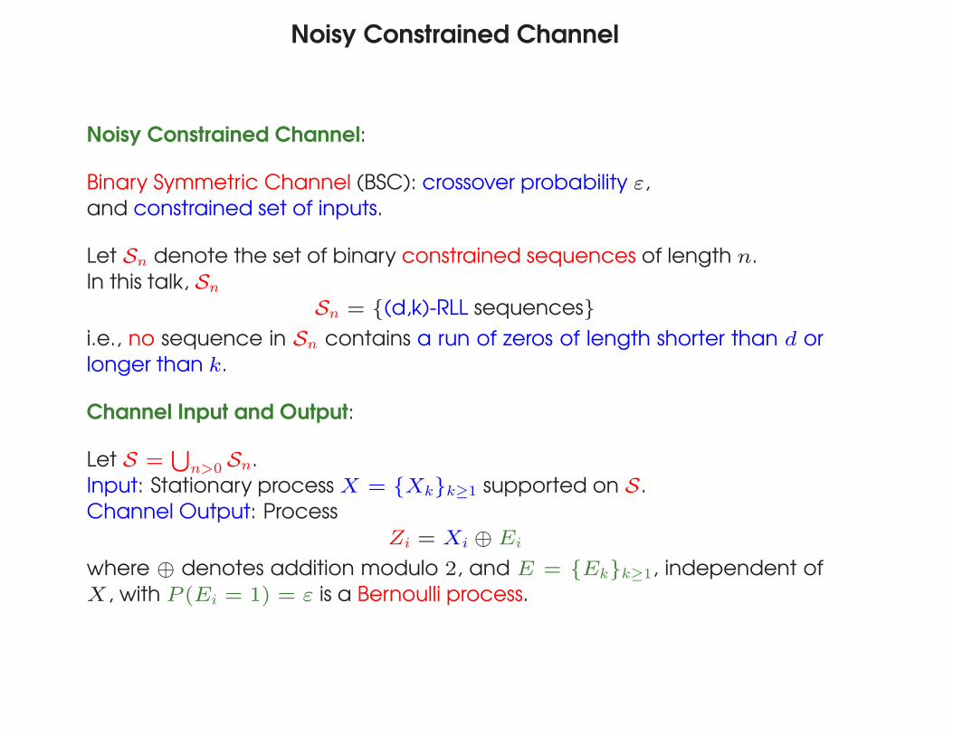
Noisy Constrained Channel

Noisy Constrained Channel:

Binary Symmetric Channel (BSC): crossover probability ε,

and constrained set of inputs.

Let Sn denote the set of binary constrained sequences of length n.

In this talk, Sn

Sn = {(d,k)-RLL sequences}i.e., no sequence in Sn contains a run of zeros of length shorter than d or

longer than k.

Channel Input and Output:

Let S =S

n>0 Sn.

Input: Stationary process X = {Xk}k≥1 supported on S.

Channel Output: Process

Zi = Xi ⊕ Ei

where ⊕ denotes addition modulo 2, and E = {Ek}k≥1, independent of

X, with P (Ei = 1) = ε is a Bernoulli process.

Noisy Constrained Capacity

C(ε) – conventional BSC channel capacity C(ε) = 1 − H(ε), where

H(ε) = −ε log ε − (1 − ε) log(1 − ε).

C(S, ε) – noisy constrained capacity defined as

C(S, ε) = supX∈S

I(X; Z) = limn→∞

1

nsup

Xn1 ∈Sn

I(Xn1 , Z

n1 ),

where the suprema are over all stationary processes supported on S and

Sn, respectively. This is an open problem since Shannon.

C(S) = C(S, 0) – noiseless capacity.

Mutual information

I(X; Z) = H(Z) − H(Z|X)

where H(Z|X) = H(ε).

We must find the entropy of H(Z), that is, the entropy of a hidden Markov

process since a (d, k) sequence can be generated as an output of a kth

order Markov process.

Hidden Markov Process

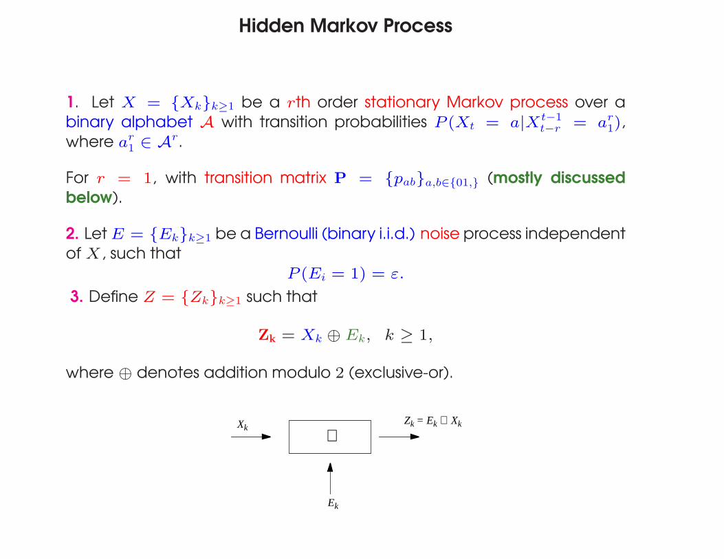
1. Let X = {Xk}k≥1 be a rth order stationary Markov process over a

binary alphabet A with transition probabilities P (Xt = a|Xt−1t−r = ar

1),

where ar1 ∈ Ar.

For r = 1, with transition matrix P = {pab}a,b∈{01,} (mostly discussed

below).

2. Let E = {Ek}k≥1 be a Bernoulli (binary i.i.d.) noise process independent

of X, such that

P (Ei = 1) = ε.

3. Define Z = {Zk}k≥1 such that

Zk = Xk ⊕ Ek, k ≥ 1,

where ⊕ denotes addition modulo 2 (exclusive-or).

Ek

Zk = Ek ⊕ XkXk ⊕

Joint Distribution of P (Zn1 )

Let X̄ = 1 ⊕ X. In particular, Zi = Xi if Ei = 0 and Zi = X̄i if Ei = 1.

We have

P (Zn1 , En) = P (Z

n1 , En−1 = 0, En) + P (Z

n1 , En−1 = 1, En)

= P (Zn−11 , Zn, En−1 = 0, En) + P (Z

n−11 , Zn, En−1 = 1, En)

= P (Zn, En|Zn−11 , En−1 = 0)P (Z

n−11 , En−1 = 0)

+P (Zn, En|Zn−11 , En−1 = 1)P (Z

n−11 , En−1 = 1)

= P (En)PX(Zn ⊕ En|Zn−1)P (Zn−11 , En−1 = 0)

+P (En)PX(Zn ⊕ En|Z̄n−1)P (Zn−11 , En−1 = 1)

Entropy as a Product of Random Matrices

Let

pn = [P (Zn1 , En = 0), P (Zn

1 , En = 1)]

and

M(Zn−1, Zn) =

»(1−ε)PX(Zn|Zn−1) εPX(Z̄n|Zn−1)

(1−ε)PX(Zn|Z̄n−1) εPX(Z̄n|Z̄n−1)

–.

Then

pn = pn−1M(Zn−1, Zn).

Since P (Zn1 ) = pn1

t (1t = (1, . . . , 1)) we finally obtain

P (Zn1 ) = p1M(Z1, Z2) · · ·M(Zn−1, Zn)1

t,

that is, product of random matrices since PX(Zi|Zi−1) are random

variables.

Entropy Rate as a Lyapunov Exponent

Theorem 1 (Furstenberg and Kesten, 1960). Let M1, . . . , Mn form a

stationary ergodic sequence and E[log+ ||M1||] < ∞ Then

limn→∞

1

nE[log ||M1 · · ·Mn||] = lim

n→∞

1

nlog ||M1 · · ·Mn|| = µ a.s.

where µ is called top Lyapunov exponent.

Corollary 1. Consider the HMP Z as defined above. The entropy rate

h(Z) = limn→∞

E[−1

nlog P (Zn

1 ) ]

= limn→∞

1

nE[− log

“p1M(Z1, Z2) · · ·M(Zn−1, Zn)1

t”]

is a top Lyapunov exponent of M(Z1, Z2) · · ·M(Zn−1, Zn).

Unfortunately, it is notoriously difficult to compute top Lyapunov

exponents as proved in Tsitsiklis and Blondel. Therefore, in next we derive

an explicit asymptotic expansion of the entropy rate h(Z).

Asymptotic Expansion

We now assume that P (Ei = 1) = ε → 0 is small.

Theorem 2. Assume rth order Markov. If the conditional symbol

probabilities in the finite memory (Markov) process X satisfy

P (ar+1|ar1) > 0

for all ar+11 ∈Ar+1, then the entropy rate of Z for small ε is

h(Z) = limn→∞

1

nHn(Z

n) = h(X) + f1(P )ε + O(ε

2),

where

f1(P ) =X

z2r+11

PX(z2r+11 ) log

PX(z2r+11 )

PX(z̄2r+11 )

= D

“PX(z2r+1

1 )||PX(z̄2r+11 )

”,

where z̄2r+1=z1 . . . zrz̄r+1zr+2 . . . z2r+1. In the above, h(X) is the entropy

rate of the Markov process X, D denotes the Kullback-Liebler divergence.

For r = 1, this result was first obtained by G. Seroussi, P. Jacquet, W.S.

(DCC’2004) (see also Ordentlich and Weissman, ISIT 2004).

Example

Consider a Markov process with symmetric transition probabilities p01 =p10 = p, p00 = p11 = 1−p. This process has stationary probabilities PX(0) =PX(1) = 1

2.

Then

h(Z) = h(X) + f1(p)ε + f2(p)ε2+ O(ε

3)

where

f1(p) = 2(1 − 2p) log1 − p

p,

f2(p) = −f1(p) − 1

2

„2p − 1

p(1 − p)

«2

.

Higher order terms obtained by Zuk, Kanter, Domany, J. Stat. Phys., 2005.

Degenerate Case

The assumption P > 0 is important.

Example: Consider (e.g., process generates (0, 1)-RLL (or (1,∞)-RLL)

sequences)

P =

»1 − p p

1 0

–

where 0 ≤ p ≤ 1.

Ordentlich and Weissman (2004) proved for this case

H(Z) = H(P ) − p(2 − p)

1 + pε log ε + O(ε)

(e.g., (11 . . .) will not be generated by MC, but can be outputed by HMM

with probability O(εκ)).

Recently, Han and Marcus (2007) showed that in general

H(Z) = H(P ) − f0(P )ε log ε + O(ε)

when at least one of the transition probabilities is zero.

If P > 0, then f0(P ) = 0 and by Theorem 2 the coefficient at ε is f1(P ).

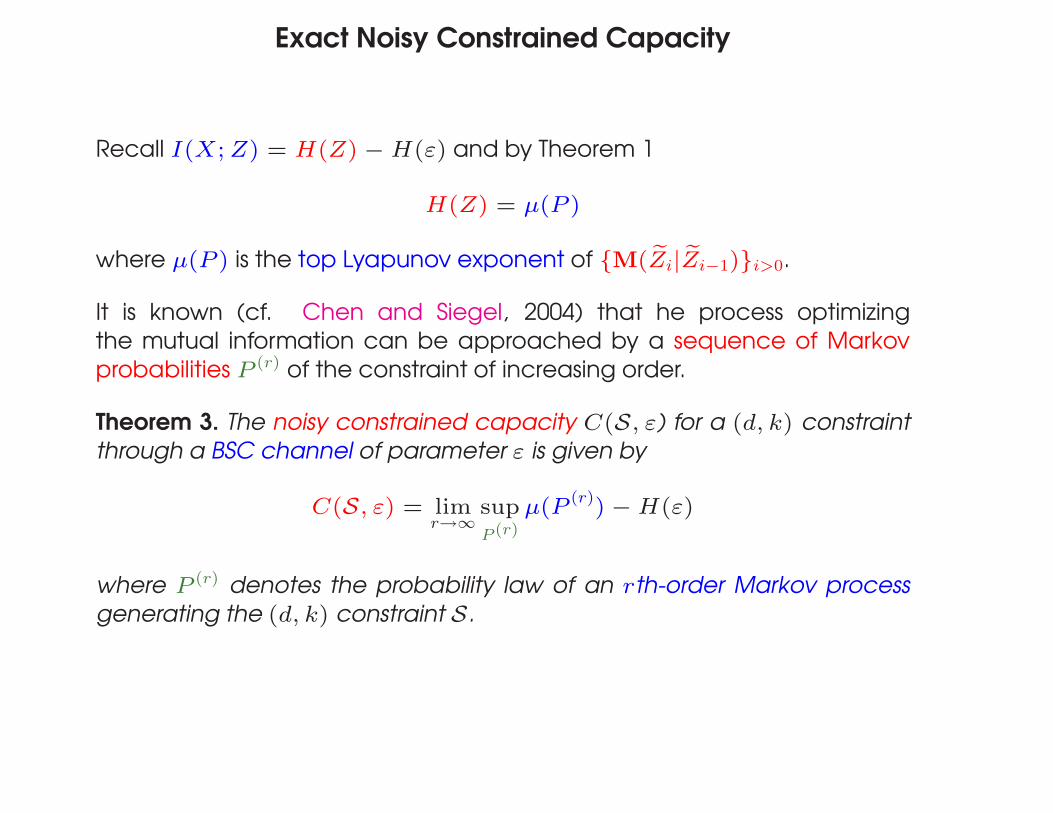
Exact Noisy Constrained Capacity

Recall I(X; Z) = H(Z) − H(ε) and by Theorem 1

H(Z) = µ(P )

where µ(P ) is the top Lyapunov exponent of {M( eZi| eZi−1)}i>0.

It is known (cf. Chen and Siegel, 2004) that he process optimizing

the mutual information can be approached by a sequence of Markov

probabilities P (r) of the constraint of increasing order.

Theorem 3. The noisy constrained capacity C(S, ε) for a (d, k) constraint

through a BSC channel of parameter ε is given by

C(S, ε) = limr→∞

supP (r)

µ(P (r)) − H(ε)

where P (r) denotes the probability law of an rth-order Markov process

generating the (d, k) constraint S.

Main Contribution – An Overview

We shall observe that

H(Z) = H(P ) − f0(P )ε log ε + f1(P )ε + o(ε)

for explicitly computable f0(P ) and f1(P ).

Let P max be the maxentropic maximizing H(P ). Following Han and Marcus

arguments we arrive at

C(S, ε)=C(S)−(1 − f0(Pmax

))ε log ε+(f1(Pmax

) − 1)ε + o(ε)

where C(S) is the capacity of noiseless RLL system.

For k ≤ 2d, we shall prove that

C(S, ε)=C(S) + A · ε + O(ε2log ε)

(i.e., ε log ε vanishes).

For k > 2d, we shall prove that

C(S, ε)=C(S) + B · ε log ε + O(ε),

where A and B are explicitly computable constants. The last result was

independently obtained by Han and Marcus (2007) using different tools.

Sketch of Proof

1. Instead of computing entropy H(Zn1 ) directly we evaluate the following

sum

R(s, ε) =X

zn1

P sZ(zn

1 ),

where s is a complex variable. Indeed,

H(Z) =∂

∂sR(s, ε)

˛̨˛̨s=1

.

2. Observe that

PZ(Zn1 ) = PX(X

n1 )(1 − ε)

n+ ε(1 − ε)

n−1nX

i=1

PX(Xn1 ⊕ ei) + O(ε

2)

where ej = (0, . . . , 0, 1, 0, . . . , 0) ∈ An with a 1 at position j.

Continuation . . .

3. Let Bn ⊆ An be the set of zn1 at Hamming distance one from Sn

Rn(s, ε) =X

zn1∈Sn

(1−ε)ns

„PX(z

n1 ) +

(∗)z }| {ε

1−ε

nX

i=1

PX(zn1⊕ei)

«s

+X

zn1∈Bn\Sn

εs(1 − ε)(n−1)s

nX

i=1

PX(zn1 ⊕ ei)

!s

+ O(ε2) .

4. Assume k ≤ 2d: a one-bit flip on a (d, k) sequence violates the

constraint, and Sn ∩ Bn = φ. The term (∗) vanishes, hence

Rn(s, ε) = Rn(s, 0)(1−ε)ns + εs(1−ε)(n−1)sQn(s) + O(ε2s),

where

Qn(s) =X

zn1∈Sn

nX

i=1

1

Ni(Xn1 )

0@

nX

j=1

P (Xn1 ⊕ ei ⊕ ej)

1A

s

where Ni(zn1 ) is the number of (d, k) sequences at Hamming distance one

from zn1 ⊕ ei.

Finishing up . . .

5. One can prove that

Qn(1) = n

and then

H(Zn1 ) = H(X

n1 ) − nε log ε − (Q

′n(1) + H(X

n1 ))ε + O(ε

2log ε)

Thus, in the case k ≤ 2d, we have f0(P ) = 1, and the term O(ε log ε)cancels out in the capacity C(S, ε).

6. To estimate Q′n(1) we consider an extended alphabet

B = { 0d1, 0d+11, . . . , 0k1 }.

and define

pℓ = P max(0ℓ1), d ≤ ℓ ≤ k .

where P max is the maxentropic distribution.

7. Define

λ =

kX

ℓ=d

(ℓ + 1)pℓ, α(s) =

kX

ℓ=d

(2d − ℓ) psℓ.

and τ(s) that is defined in the paper.

Final Results

Theorem 4. Consider the constrained system S with k ≤ 2d. Then,

C(S, ε) = C(S) − (2 − τ ′(1) + α′(1)

λ)ε + O(ε2 log ε) .

Here, the derivatives of α and τ are with respect to s, evaluated at s=1.

We can extend it to k > 2d.

Theorem 5. Consider the constrained system S with k ≥ 2d. Define

γ =X

ℓ>2d

(ℓ − 2d)pℓ , δ =X

ℓ1+ℓ2+1≤k

pℓ1pℓ2

.

Then

C(S, ε) = C(S) − (1 − f0(Pmax

)) ε log ε−1

+ O(ε) ,

where f0(Pmax) = 1 − γ + δ

λ.

Example

We consider the (1,∞) or (0, 1) constraint with transition matrix P as in

Ordentlich and Weissman.

Setting in previous Theorem for d = 1 and k = ∞, we obtain

pℓ = (1 − p)ℓ−1p, λ =1 + p

p, γ =

(1 − p)2

p.

and δ = 1. Thus,

f0(P ) = 1 − γ + δ

λ=

p(p − 2)

p − 1,

as before.

The noisy constrained capacity is obtained when p = 1/ϕ2, where ϕ =(1 +

√5)/2, the golden ratio, and

f0(Pmax) = 1/

√5

and the coefficient at ε log(1/ε) is (1/√

5)−1 ≈ −0.553.