Noisy entanglement evolution for graph states

L. Aolita,1 D. Cavalcanti,2 R. Chaves,3 C. Dhara,1 L. Davidovich,3 and A. Acın1, 4, ∗

1ICFO-Institut de Ciencies Fotoniques, Mediterranean Technology Park, 08860 Castelldefels (Barcelona), Spain2Centre for Quantum Technologies, University of Singapore, Singapore

3Instituto de Fısica, Universidade Federal do Rio de Janeiro. Caixa Postal 68528, 21941-972 Rio de Janeiro, RJ, Brasil4ICREA-Institucio Catalana de Recerca i Estudis Avancats, Lluis Companys 23, 08010 Barcelona, Spain

A general method for the study of the entanglement evolution of graph states under the actionof Pauli was recently proposed in [Cavalcanti, et al., Phys. Rev. Lett. 103, 030502 (2009)]. Thismethod is based on lower and upper bounds on the entanglement of the entire state as a function onlyof the state of a considerably-smaller subsystem, which undergoes an effective noise process. Thisprovides a huge simplification on the size of the matrices involved in the calculation of entanglementin these systems. In the present paper we elaborate on this method in details and generalize it toother natural situations not described by Pauli maps. Specifically, for Pauli maps we introduce anexplicit formula for the characterization of the resulting effective noise. Beyond Pauli maps, we showthat the same ideas can be applied to the case of thermal reservoirs at arbitrary temperature. In thelatter case, we discuss how to optimize the bounds as a function of the noise strength. We illustrateour ideas with explicit exemplary results for several different graphs and particular decoherenceprocesses. The limitations of the method are also discussed.

PACS numbers: 03.67.-a, 03.67.Mn, 03.65.Yz

I. INTRODUCTION

Graph states [1] constitute an important family of gen-uine multiparticle-entangled states with several applica-tions in quantum information. The most popular ex-ample of these are arguably the cluster states, whichhave been identified as a crucial resource for universalmeasurement-based quantum computation [2, 3]. Othermembers of this family were also proven to be potentialresources, as codewords for quantum error correction [4],to implement secure quantum communication [5], andto simulate some aspects of the entanglement distribu-tion of random states [6]. Moreover, graph states encom-pass the celebrated Greenberger-Horne-Zeilinger (GHZ)states [7], whose importance ranges from fundamental toapplied issues. GHZ states can – for large-dimensionalsystems – be considered as simple models of the gedankenSchrodinger-cat states, are crucial for quantum commu-nication protocols [8], and find applications in quantummetrology [9] and high-precision spectroscopy [10]. Allthese reasons explain the great deal of effort made bothto theoretically understand the features [1], and to gen-erate and coherently manipulate graph states in the lab-oratory [11].

For the same reasons, it is crucial to unravel the dy-namics of graph states in realistic scenarios, where thesystem is unavoidably exposed to interactions with its en-vironment and/or experimental imperfections. Previousstudies on the robustness of graph-state entanglement inthe presence of decoherence showed that the disentan-

∗Electronic address: antonio.acin@icfo.es

glement times (i.e. the time for which the state becomesseparable) increases with the system size [12, 13]. How-ever the disentanglement time on its own is known not toprovide in general a faithful figure of merit for the entan-glement robustness: although the disentanglement timecan grow with the number N of particles, the amountof entanglement in a given time can decay exponentiallywith N [14]. The full dynamical evolution must then bemonitored to draw any conclusions on the entanglementrobustness.

A big obstacle must be overcome in the study of en-tanglement robustness in general mixed states: the directquantification of the entanglement involves optimizationsrequiring computational resources that increase exponen-tially with N . The problem thus becomes in practiceintractable even for relatively small system sizes, not tomention the direct assessment of entanglement during theentire noisy dynamics. All in all, some progress has beenachieved in the latter direction for some very particu-lar cases: For arbitrarily-large linear-cluster states undercollective dephasing, it is possible to calculate the ex-act value of the geometric measure of entanglement [15]throughout the evolution [16]. Besides, bounds to therelative entropy and the global robustness of entangle-ment for two-colorable graph states [1] of any size underlocal dephasing were obtained [17].

In a conceptually different approach, a framework toobtain families of lower and upper bounds to the entan-glement evolution of graph, and graph-diagonal, statesunder decoherence was introduced in Ref. [18]. Thebounds are obtained via a calculation that involves onlythe boundary subsystem, composed of the qubits lying atthe boundary of the multipartition under scrutiny. This,very often, reduces considerably the size of the matrices

arX

iv:1

006.

3152

v1 [

quan

t-ph

] 1

6 Ju

n 20

10

2

involved in the calculation of entanglement. No opti-mization on the full system’s parameter space is requiredthroughout. Another remarkable feature of the method isthat it is not limited to a particular entanglement quanti-fier but applies to all convex (bi-or multi-partite) entan-glement measures that do not increase under local oper-ations and classical communication (LOCC). The latterare indeed two rather natural and general requirements[19].

In the case of open-dynamic processes described byPauli maps, which are defined below, the lower and upperbounds coincide and the method thus allows one to calcu-late the exact entanglement of the noisy evolving state.Pauli maps encompass popular models of (independentor collective) noise, as depolarization, phase flip, bit flipand bit-phase flip errors, and are defined below. More-over, one of the varieties of lower bounds is of extremelysimple calculation and – despite less tight – depends onlyon the connectivity of the graph and not on its total size.The latter is a very advantageous property in situationswhere one wishes to assess the resistance of entanglementwith growing system size. For example, the versatility ofthe formalism has very recently been demonstrated inRef. [20], where it was applied to demonstrate the ro-bustness of thermal bound entanglement in macroscopicmany-body systems of spin-1/2 particles.

In the present paper, we elaborate on the details of theformalism introduced in [18]. For Pauli maps we give anexplicit formula for the characterization of the effectivenoise involved in the calculation of the bounds. Further-more, we extend the method to the case where each qubitis subjected to the action of independent thermal baths ofarbitrary temperature. This is a crucial, realistic type ofdynamic process that is not described by Pauli maps. Inall cases, we exhaustively compare the different boundswith several concrete examples. Finally, we discuss themain advantages and limitations of our method in com-parison with other approaches.

The article is organized as follows:

• Sec. II: here we define the notation, introduce def-initions and review basic concepts required in thefollowing sections. In particular, graph and graph-diagonal states are defined in subsection II A andthe noise models considered are presented in sub-section II B.

• Sec. III: a detailed description of the proposedframework is given in the context of a fully gen-eral noise. Families of lower and upper bounds forthe entanglement evolution in a chosen partitionin terms of that of the boundary subsystem aloneunder an effective noise are provided.

• Sec. IV: the developed machinery is applied tothe case of noises described by arbitrary Paulimaps and diffusion and dissipation with indepen-dent thermal reservoirs at any temperature. Ex-act results for the entanglement decay are obtained

for Pauli maps, whereas optimized bounds are pro-vided in the other cases.

• Sec. V: we first discuss how the method can beextended to other initial states or decoherence pro-cesses. In particular, how non-tight lower boundsfor the entanglement evolution of any initial statesubjected to any decoherence process can be ob-tained. Then we comment on the limitations of themethod.

• Sec. VI: we conclude the paper with a summary ofthe results and their physical implications.

II. BASIC CONCEPTS

In this section, we define graph and graph-diagonalstates, introduce the basics of open-system dynamics andthe particular noise models used later.

A. Graph and graph-diagonal states

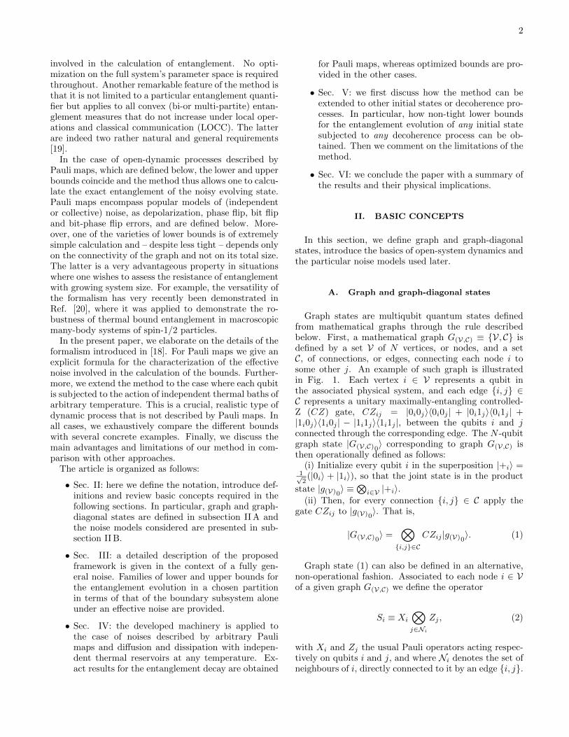
Graph states are multiqubit quantum states definedfrom mathematical graphs through the rule describedbelow. First, a mathematical graph G(V,C) ≡ {V, C} isdefined by a set V of N vertices, or nodes, and a setC, of connections, or edges, connecting each node i tosome other j. An example of such graph is illustratedin Fig. 1. Each vertex i ∈ V represents a qubit inthe associated physical system, and each edge {i, j} ∈C represents a unitary maximally-entangling controlled-Z (CZ) gate, CZij = |0i0j〉〈0i0j | + |0i1j〉〈0i1j | +|1i0j〉〈1i0j | − |1i1j〉〈1i1j |, between the qubits i and jconnected through the corresponding edge. The N -qubitgraph state |G(V,C)0〉 corresponding to graph G(V,C) isthen operationally defined as follows:

(i) Initialize every qubit i in the superposition |+i〉 =1√2(|0i〉 + |1i〉), so that the joint state is in the product

state |g(V)0〉 ≡⊗

i∈V |+i〉.(ii) Then, for every connection {i, j} ∈ C apply the

gate CZij to |g(V)0〉. That is,

|G(V,C)0〉 =⊗{i,j}∈C

CZij |g(V)0〉. (1)

Graph state (1) can also be defined in an alternative,non-operational fashion. Associated to each node i ∈ Vof a given graph G(V,C) we define the operator

Si ≡ Xi

⊗j∈Ni

Zj , (2)

with Xi and Zj the usual Pauli operators acting respec-tively on qubits i and j, and where Ni denotes the set ofneighbours of i, directly connected to it by an edge {i, j}.

3

FIG. 1: (Color online.) Mathematical graph associated to agiven physical graph state. An exemplary bipartition dividesthe system into two subparts: the yellow and white regions.The edges in black are the boundary-crossing edges X andthe nodes (also in black) connected by these are the bound-ary nodes Y. Together they compose the boundary sub-graphG(Y,X ). The remaining vertices, painted in orange, consti-tute the non-boundary subsystem.

Operator (2) possess eigenvalues 1 and −1. It is the i-thgenerator of the stabilizer group and is often called forshort stabilizer operator. All N stabilizer operators com-mute and share therefore a common basis of eigenstates.Graph state |G(V,C)0〉 in turn has the peculiarity of being

the unique common eigenstate of eigenvalue +1 [1]. Inother words,

Si|G(V,C)0〉 = |G(V,C)0〉 ∀ i ∈ V.

The other 2N − 1 common eigenstates |G(V,C)ν〉 are in

turn related to (1) by a local unitary operation:

|G(V,C)ν〉 =⊗i∈V

Ziνi |G(V,C)0〉 = Zν |G(V,C)0〉, (3)

such that Si∣∣G(V,C)ν

⟩=(−1)

νi∣∣G(V,C)ν

⟩, where ν is a

multi-index representing the binary string ν ≡ ν1 ... νN ,with νi = 0 or 1 ∀ i ∈ V, and where the short-handnotation Zν ≡

⊗i∈V Zi

νi has been introduced. There-fore, states (3) possess all exactly the same entanglementproperties and, together with |G(V,C)0〉, define the com-

plete orthonormal graph-state basis of H (correspondingto the graph G(V,C)). Any state ρ diagonal in such basisis called a graph-diagonal state:

ρGD =∑ν

Pν |G(V,C)ν〉〈G(V,C)ν |, (4)

where pν is any probability distribution. Interestingly,for any graph, any arbitrary N -qubit state can always be

depolarized by some separable map (defined below) intothe form (4) without changing its diagonal elements inthe considered graph basis [21].

Two simple identities following from definition (2)will be crucial for our purposes. For every eigenstate|G(V,C)ν〉 of Si, with eigenvalues siν = 1 or −1

Xi|G(V,C)ν〉 = Si ⊗⊗j∈Ni

Zj |G(V,C)ν〉

= siν⊗j∈Ni

Zj |G(V,C)ν〉, (5)

where definition (2) was used, and

Yi|G(V,C)ν〉 = (−i)Zi.Si ⊗⊗j∈Ni

Zj |G(V,C)ν〉

= siν(−i)Zi ⊗⊗j∈Ni

Zj |G(V,C)ν〉. (6)

So, when applied to any pure graph – or mixed graph-diagonal – state, the following operator equivalences holdup to a global phase:

Xi ↔⊗j∈Ni

Zj , (7a)

Yi ↔ Zi ⊗⊗j∈Ni

Zj . (7b)

B. Open-system dynamics

As we mentioned in Sec. I, our ultimate goal is tostudy the behavior of graph state entanglement in real-istic dynamic scenarios where the system evolves duringa time interval t according to a generic physical process,which can include decoherence. This process can alwaysbe represented by a completely-positive trace-preservingmap Λ, that maps any initial state ρ to the evolved oneafter a time t, ρt ≡ Λ(ρ). In turn, for every such Λ, therealways exists a maximum of D2 (D = dim(H)) operatorsKµ such that the map is expressed in a Kraus form [22].

ρt ≡ Λ(ρ) =∑µ

KµρK†µ. (8)

Operators Kµ are called the Kraus operators, and de-compose the identity operator 1 of H in the followingmanner:

∑µK

†µKµ = 1. Conversely, the Kraus repre-

sentation encapsulates all possible physical dynamics ofthe system. That is, any map expressible as in (8) isautomatically completely-positive and trace-preserving.For our case of interest – N -qubit systems –, index µ

runs from 0 to (2N )2 − 1 = 4N − 1. For later conve-

nience, we will represent it in base 4, decomposing it asthe following multi-index: µ ≡ µ1 ... µN , with µi = 0, 1,2, or 3 ∀ i ∈ V.

We call Λ a separable map with respect to some mul-tipartition of the system if each and all of its Kraus

4

operators factorize as tensor products of local operatorseach one with support on only one of the subparts. Forexample, if we split the qubits associated to the graphshown in Fig. 1 into a set Y of boundary qubits (in black)and its complement Y ≡ V/Y of non-boundary qubits (ingreen), Λ is separable with respect to this partitioning ifKµ ≡ KYµ ⊗KYµ, with KYµ and KYµ operators acting

non-trivially only on the Hilbert spaces of the boundaryand non-boundary qubits, respectively. By definition, aseparable map cannot increase the entanglement in theconsidered multipartition.

In turn, we call Λ an independent map with respect tosome multipartition of the system if it can be factorizedas the composition (tensor product) of individual mapsacting independently on each subpart. Otherwise, we saythat Λ is a collective map. Examples of fully independentmaps are those in which each qubit i is independentlysubject to its own local noise channel Ei. By the termindependent map without explicit mention to any respec-tive multipartition we will refer throughout to fully inde-pendent maps. In this case, the global map Λ factorizescompletely:

Λ(ρ) = E1 ⊗ E2 ⊗ . . .⊗ EN (ρ). (9)

It is important to notice that all independent maps arenecessarily separable but a general separable map doesnot need to be factorable as in (9) and can therefore beboth, either individual or collective.

1. Pauli maps

A crucial family of fully separable maps is that ofthe Pauli maps, for which every Kraus operator is pro-portional to a product of individual Pauli and iden-tity operators acting on each qubit. That is, Kµ ≡√P(µ1, ... µN ) σ1µ1

⊗. . .⊗σNµN≡√Pµ σµ, with σi0 = 1i

(the identity operator on qubit i), σi1 = Xi, σi2 = Yi,and σi3 = Zi, and P(µ1, ... µN ) ≡ Pµ any probabilitydistribution. Popular instances are the (collective orindependent) depolarization and dephasing (also calledphase damping, or phase-flip) maps, and the (individ-ual) bit-flip and bit-phase-flip channels [22]. For exam-ple, the independent depolarizing (D) channel describesthe situation in which the qubit remains untouched withprobability 1 − p, or is depolarized - meaning that it istaken to the maximally mixed state (white noise) - withprobability p. It is characterized by the fully-factorableprobability Pµ = p1µ1

× ... pNµN, with pi0 = 1 − p

and pi1 = pi2 = pi3 = p/3, ∀ i ∈ V. The indepen-dent phase damping (PD) channel in turn induces thecomplete loss of quantum coherence with probability p,but without any energy (population) exchange. It is alsogiven by a fully-factorable probability with pi0 = 1−p/2,pi1 = 0 = pi2, and pi3 = p/2, ∀ i ∈ V.

For later convenience, we finally recall that eachPauli operator σiµi

can be written in the following way

(also called the chord representation [28]): Ti(ui,vi) ≡Zvii .X

uii , with ui and vi = 0, or 1. Indeed, notice that

σi2vi+|vi+ui|2 = Ti(ui,vi) (up to an irrelevant phase factorfor ui = 1 = vi), where “| |2” stands for modulo 2. In thisrepresentation, the Kraus decomposition of the above-considered general Pauli map has the following Kraus op-erators: KC (U,V ) ≡

√PC(u1,v1, ... uN ,vN ) T1(u1,v1)⊗ . . .⊗

TN (uN ,vN ) ≡√PC(U,V ) T(U,V ), where U ≡ (u1, ... uN )

and V ≡ (v1, ... vN ). The probability PC(U,V ) ≡PC(u1,v1, ... uN ,vN ) in turn is related to the original Pµ byPC(u1,v1, ... uN ,vN ) ≡ P(2v1+|v1+u1|2, ... ,2vN+|vN+uN |2)).

2. The thermal bath case

An important example of a non-Pauli, indepen-dent map is the generalized amplitude-damping channel(GAD) [22]. It represents energy diffusion and dissipa-tion with a thermal bath into which each qubit is indi-vidually immersed. Its Kraus representation is

Kiµi=0 ≡√

n+ 1

2n+ 1(|0i〉〈0i|+

√1− p|1i〉〈1i|), (10a)

Kiµi=1 ≡√

n+ 1

2n+ 1p|0i〉〈1i|, (10b)

Kiµi=2 ≡√

n

2n+ 1(√

1− p|0i〉〈0i|+ |1i〉〈1i|), (10c)

and

Kiµi=3 ≡√

n

2n+ 1p|1i〉〈0i|. (10d)

Here n is the average number of quanta in the thermalbath, p ≡ p(t) ≡ 1− e− 1

2γ(2n+1)t is the probability of thequbit exchanging a quantum with the bath after a timet, and γ is the zero-temperature dissipation rate. Chan-nel GAD is actually the extension to finite temperatureof the purely dissipative amplitude damping (AD) chan-nel, which is obtainen from GAD in the zero-temperaturelimit n = 0. In the opposite extreme, the purely diffu-sive case is obtained from GAD in the composite limitn → ∞, γ → 0, and nγ = Γ, where Γ is the diffusionconstant. Note that in the purely-diffusive limit channelGAD becomes a Pauli channel, with defining individualprobabilities pi0 = 1

2 (1 − p/2 +√

1− p), pi1 = p4 = pi2,

and pi3 = 12 (1− p/2−

√1− p), ∀ i ∈ V.

Finally, the probability p in channels D, PD and GADabove can be interpreted as a convenient parametrizationof time, where p = 0 refers to the initial time 0 and p = 1refers to the asymptotic t→∞ limit.

III. EVOLUTION OF GRAPH-STATEENTANGLEMENT UNDER GENERIC NOISE

As mentioned before, the direct calculation of the en-tanglement in arbitrary mixed states is a task exponen-

5

tially hard in the system’s size [19]. In this section, weelaborate in detail a formalism that dramatically sim-plifies this task for graph – or graph-diagonal – statesundergoing a noisy evolution in a fully general context.Along the way, we also describe carefully which require-ments an arbitrary noisy map has to satisfy so that theformalism can be applied.

A. The general idea

Consider a system initially in graph state (1) thatevolves during a time t according to the general map(8) towards the evolved state

ρt ≡ Λ(|G(V,C)0〉) =∑µ

Kµ|G(V,C)0〉〈G(V,C)0|K†µ. (11)

We would like to follow the entanglement E(ρt) of ρtduring its entire evolution. Here, E is any convex en-tanglement monotone [19] that quantifies the entangle-ment content in some given multi-partition of the sys-tem. An example of such multi-partition is displayed inFig. 1, where the associated graph is split into two sub-sets, painted respectively in yellow and white in the fig-ure. The edges that connect vertices at different subsetsare called the boundary-crossing edges and are painted inblack in the figure. We call the set of all the boundary-crossing edges X ⊆ C, and its complement X ≡ C/X theset of all non-boundary-crossing edges. All the qubitsassociated to vertices connected by any edge in X con-stitute the set Y ⊆ V of boundary qubits (or boundarysubsystem), and its complement Y ≡ V/Y is the non-boundary qubit set. We refer to G(Y,X ) as the boundarysub-graph.

We can use this classification and the operational def-inition (1) to write the initial graph state as

|G(V,C)0〉 =⊗{i,j}∈X

CZij |G(Y,X )0〉 ⊗ |g(Y)0〉, (12)

where |g(Y)0〉 ≡⊗

i∈Y |+i〉. In other words, we explic-

itly factor out all the CZ gates corresponding to non-boundary qubits.

Consider now the application of some Kraus op-erator Kµ of a general map on graph state (12):Kµ

⊗{i,j}∈X CZij |G(Y,X )0

〉 ⊗ |g(Y)0〉. The latter can al-

ways be written as⊗{i,j}∈X CZijKµ|G(Y,X )0

〉 ⊗ |g(Y)0〉,with

Kµ =⊗{i,j}∈X

CZij Kµ

⊗{i′,j′}∈X

CZi′j′ , ∀ µ, (13)

Now, consider every map Λ such that transformation rule(13) yields, for each and all of its Kraus operators, mod-ified Kraus operators of the form

Kµ = KYγ ⊗ KYω, (14)

where KYγ and KYω are normalized (modified) Krausoperators acting non-trivially only on the boundary andnon-boundary qubits, respectively, and γ = {µi, i ∈ Y}and ω = {µi, i ∈ Y} are multi-indices labeling re-spectively the alternatives for the boundary and non-boundary subsystems. The modified map Λ, composedof Kraus operators Kµ is then clearly bi-separable withrespect to the bi-partition “boundary / non-boundary”.For all such maps the calculation of E(ρt) can be drasti-cally simplified, as we see in what follows.

In these cases, the evolved state (11) can be writen as

ρt ≡ Λ(|G(V,C)0〉) =⊗{i,j}∈X

CZij ρt⊗{k,l}∈X

CZkl. (15)

with

ρt = Λ(|G(Y,X )0〉 ⊗ |g(Y)0〉) =

∑µ

KYγ(µ)|G(Y,X )0〉〈G(Y,X )0

|K†Yγ(µ) ⊗ KYω(µ)|g(Y)0〉〈g(Y)0|K†Yω(µ)

=∑ω

KYω|g(Y)0〉〈g(Y)0|K†Yω ⊗

∑γ

KY(γ|ω)|G(Y,X )0〉〈G(Y,X )0

|K†Yγ , (16)

where KY(γ|ω) is the γ-th modified Kraus operator on the

boundary subsystem given that KYω has been applied tothe non-boundary one. Recall that both γ ≡ γ(µ) andω ≡ ω(µ) come from the same single multi-index µ andare therefore in general not independent on one another.In the second equality of (16) we have chosen to treat ω

as an independent variable for the summation and makeγ explicitly depend on ω. This can always be done andwill be convenient for our purposes.

The crucial observation now is that the CZ operatorsexplicitly factored out in the evolved state (15) corre-spond to non-boundary-crossing edges. Thus, they act

6

as local unitary operations with respect to the multi-partition of interest. For this reason, and since local uni-tary operations do not change the entanglement contentof any state, the equivalence

E(ρt) = E(ρt) (17)

holds.In the forthcoming subsections we see how, by exploit-

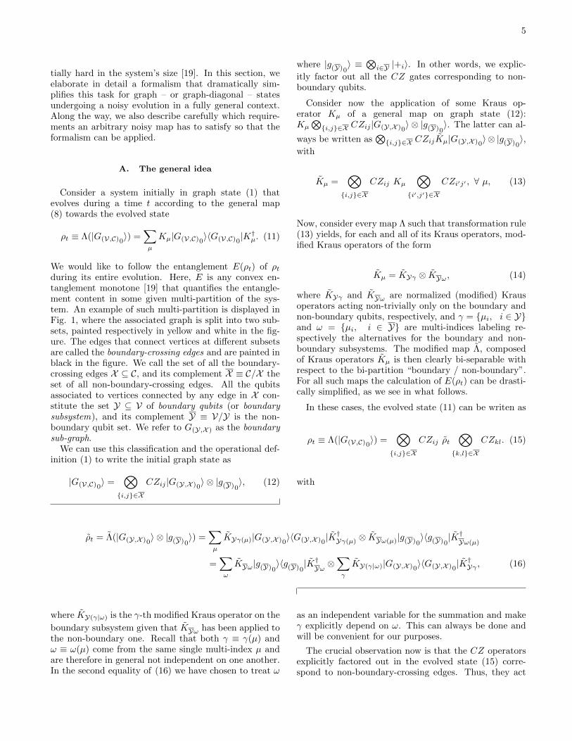
ing this equivalence in different noise scenarios, the com-putational effort required for a reliable estimation (andin some cases, an exact calculation) of E(ρt) can be con-siderably reduced. The main idea behind this reductionlies on the fact that, whereas in the general expression(11) the entanglement can be distributed among all par-ticles in the graph, in state (16) the boundary and non-boundary subsystems are explicitly in a separable state.All the entanglement in the multi-partition of interest istherefore localized exclusively in the boundary subgraph.The situation is graphically represented in Fig. 2, wherethe same graph as in Fig. 1 is plotted but with all itsnon-boundary-crossing edges erased.

FIG. 2: (Colour online.) Same graph as in Fig. 1 but where allnon-boundary-crossing edges have been erased, representingthe fact that the boundary and non-boundary subsystems arefully unentangled. The entanglement in the whole system isobtained via a calculation involving only the smaller boundarysubsystem.

More precisely, the general approach consists of ob-taining lower and upper bounds on E(ρt) by boundingthe entanglement of state (16) from above and below asexplained in what follows.

1. Lower bounds to the entanglement evolution

The property of LOCC monotonicity of E, whichmeans that the average entanglement cannot grow during

an LOCC process [27], allows us to derive lower-boundson E(ρt). The ones we consider can be obtained by thefollowing generic procedure:

(i) after bringing the studied state into the form(16), apply some local general measurement M ={Mω′}, with measurement elements Mω, on thenon-boundary subsystem Y;

(ii) for each measurement outcome ω trace out the mea-sured non-boundary subsystem, and finally

(iii) calculate the mean entanglement in the resultingstate of the boundary subsystem Y, averaged overall outcomes ω.

Since this procedure constitutes an LOCC with respectto the multipartition under scrutiny, the latter averageentanglement can only be smaller than, or equal to, thatof the initial state, i.e. :

E(ρt) = E(ρt) ≥∑ω

PωE(∑

ω′

1

Pω〈g(Y)0|K

†Yω′M

†ω.MωKYω′ |g(Y)0〉

∑γ

KY(γ|ω′)|G(Y,X )0〉〈G(Y,X )0

|K†Y(γ|ω′)

). (18)

with Pω ≡∑ω′〈g(Y)0|K

†Yω′M

†ω.MωKYω′ |g(Y)0〉 being the

probability of outcome ω.

Notice that if the states {KYω′ |g(Y)0〉} of

the non-boundary subsystem happen to be or-

7

thogonal, then there exists an optimal mea-

surement M = {Mω ≡KYω|g(Y)0

〉〈g(Y)0|K†

Yω

〈g(Y)0|K†

YωKYω|g(Y)0

〉}

that can distinguish them unambiguously, so

that 〈g(Y)0|K†Yω′M

†ω.MωKYω′ |g(Y)0〉 = δω,ω′ ×

〈g(Y)0|K†YωKYω|g(Y)0〉 and Pω = 〈g(Y)0|K

†YωKYω|g(Y)0〉.

In these cases an optimal lower bound is achieved as(constant normalization factors omitted again)

E(ρt) ≥∑ω

PωE(∑

γ

KY(γ|ω)|G(Y,X )0〉〈G(Y,X )0

|K†Y(γ|ω)). (19)

Full distinguishability of the states in the non-boundarysubsystem allows to reduce the mixing in the remainingboundary subsystem. In other words, the measurementoutcome ω works as a perfect flag that marks which sub-ensemble of states of the boundary subsystem, from allthose present in mixture (16), corresponds indeed to theobtained outcome.

In the opposite extreme, when states {KYω′ |g(Y)0〉}are all equal, no flagging information can be obtainedvia any measurement. In this case, the resulting boundis always equal to that obtained had we not made anymeasurement at all, but just directly taken the partialtrace over Y from (16):

E(ρt) ≥

E( 1

2|Y|

∑ω,γ

KY(γ|ω)|G(Y,X )0〉〈G(Y,X )0

|K†Y(γ|ω)). (20)

where |Y| stands for the number of non-boundary qubitsand full mixing over variable ω takes place now.

Henceforth we refer to lower bound (20) as the lowestlower bound (LLB). As its name suggests, its tightnessis far from the optimal one given by (19). However, aswe will see in the forthcoming subsections, due to thepartial tracing, it typically does not depend on the totalsystem’s size but just on the boundary subsystem’s.

This constitutes an appealing, useful property, for itallows one to draw generic conclusions about the robust-ness of entanglement in certain partitions of graph states,irrespective of their number of constituent particles (seeexamples below).

2. Upper bounds to the entanglement evolution

On the other hand, we consider upper-bounds on E(ρt)based on the property of convexity of E, which essentiallymeans that the entanglement of the convex sum is lowerthan, or equal to, the convex sum of the entanglements[19]. From (16), the latter implies that

E(ρt) = E(ρt) ≤∑ω

PωE( 1

PωKYω|g(Y)0〉〈g(Y)0|K

†Yω ⊗

∑γ

KY(γ|ω)|G(Y,X )0〉〈G(Y,X )0

|K†Y(γ|ω)), (21)

where, once again, Pω = 〈g(Y)0|K†YωKYω|g(Y)0〉. In

each term of the last summation the boundary andnon-boundary subsystems inside the brackets are ina product state. Therefore, as for what the multi-partition of interest concerns, the non-boudary sub-system works as a locally-added ancila (in a state1PωKYω|g(Y)0〉〈g(Y)0|K

†Yω) and consequently does not

have any influence on the amount of entanglement. Thisleads to the generic upper bound

E(ρt) ≤∑ω

PωE(∑

γ

KY(γ|ω)|G(Y,X )0〉〈G(Y,X )0

|K†Y(γ|ω)). (22)

3. Exact entanglement

Notice that upper bound (22) and optimal lower bound(19) coincide. This means that, in the above-mentioned

case when states {KYω|g(Y)0〉} are orthogonal, these co-

incident bounds yield actually the exact value of E(ρt):

E(ρt) =∑ω

PωE(∑

γ

KY(γ|ω)|G(Y,X )0〉〈G(Y,X )0

|K†Y(γ|ω)). (23)

Expression (23) is still not an analytic closed formulafor the exact entanglement of ρt, but reduces its calcula-tion to that of the average entanglement over an ensem-ble of states of the boundary subsystem alone. More indetail, a brute-force calculation of E(ρt) would require

8

in general a convex optimization over the entire (2N )2-

complex-parameter space. Through Eq. (23) in turnsuch calculation is reduced to that of the average en-

tanglement over a sample of 2|Y| states (one for each ω)of |Y| qubits, being |Y| the number of boundary qubits.

The latter involves at most 2|Y| independent optimiza-

tions over a (2|Y|)2-complex-parameter space. This, from

the point of view of computational memory required, ac-

counts for a reduction of resources by a factor of (2|Y|)2.

Alternatively, when computational memory is not a ma-jor restriction – for example if large classical-computerclusters are at hand –, one can take advantage of thefact that the |Y| required optimizations in (23) are in-dependent and therefore the calculation comes readilyperfectly-suited for parallel computing. In this case,it is in the required computational time where an |Y|-exponentially large speed-up is gained.

In the cases where states {KYω|g(Y)0〉} are not orthog-

onal and the upper and lower bounds do not coincide,expressions (22) and (18) still yield highly non-trivial up-per and lower bounds, respectively, as we discuss in Sec.IV B.

Finally, it is important to stress that all the bounds de-rived here are general in the sense that they hold for anyfunction fulfilling the fundamental properties of convex-ity and monotonicity under LOCC processes. This classincludes genuine multipartite entanglement measures, aswell as several quantities designed to quantify the useful-ness of quantum states in the fulfillment of some giventask for quantum-information processing or communica-tion [19].

IV. GRAPH STATES UNDER PAULI MAPS ORTHERMAL RESERVOIRS

In the present section we apply the ideas of the previ-ous section to some important concrete examples of noiseprocesses. This shows how the method is helpful in theentanglement calculation for systems in natural dynam-ics physical scenarios. We first discuss the case of Paulimaps and then the generalized amplitude damping chan-nel (thermal reservoir). Explicit calculations for noisygraph states composed of up to fourteen qubits are pre-sented as examples.

A. Pauli maps on graph states

Pauli maps defined in Sec. II B provide the most im-portant and general subfamily of noise types for whichexpression (23) for the exact entanglement of the evolvedstate applies. In this case, every Xi or Yi Pauli matrixin the map’s Kraus operators is systematically substi-tuted by products of Zi and 1i according to rules (7).

The resulting map Λ defined in this way automatically

commutes with any CZ gate and is fully separable, sothat condition (14) is trivially satisfied. Since for everyqubit in the system four orthogonal single qubit opera-tors are mapped into products of just two, several differ-ent Kraus operators of the original map contribute to thesame Kraus operator of the modified one. This allows usto simplify the notation going from indices µi, which runover 4 possible values each, to modified indices µi hav-ing only two different alternatives. In fact, the originaloperators Kµ give rise to only 2N modified ones of theform

Kµ =

√PµZ

µ1

1 ⊗ Zµ2

2 ⊗ · · · ⊗ ZµN

N ≡√PµZ

µ (24)

where multi-index µ stands for the binary string µ =µ1 . . . µN , with µi = 0 or 1, ∀i ∈ V. Probability Pµ isgiven simply by the summation of all Pµ in the originalPauli map over all the different events µ for which σµyields – via rules (7) – the same modified operator Zµ in(24).

To compute the latter modified probability we moveto the chord notation [28], mentioned at the end of Sec.II B 1. Indeed, under transformation (7), we have thatTi(ui,vi) → Zvi1i ⊗

⊗j∈Ni

Zuij , so that T(U,V ) ≡ T1(u1,v1)⊗

... TN (uN ,vN ) → Zv1+

∑j∈N1

uj

1 ⊗ · · · ⊗ ZvN+

∑j∈NN

uj

N .

The latter coincides with Zµ every time µi = |vi +∑j∈Ni

uj |2, ∀ i ∈ V. Thus, in this representation, the

modified probability PCµ is obtained from the definingprobability PC(U,V ) in the original map by the explicitformula

PCµ ≡∑U

PC(u1,|µ1−∑

j∈N1uj |2, ... ,uN ,|µ1−

∑j∈NN

uj |2).

(25)The modified Kraus operators (24) in turn are fully

separable, thus trivially satisfying factorization condition(14). We can express them as Kµ = KYγ ⊗ KYω, with

KYγ ≡ KY(γ|ω) =√P(γ|ω)Z

γ and KYω =

√PωZ

ω.

(26)The new multi-indices are γ = {µi, i ∈ Y} and ω ={µi, i ∈ Y}, and the corresponding probabilities satisfy

P(γ|ω)Pω ≡ Pµ.

The states {KYω′ |g(Y)0〉 =√Pω′Zω

′ |+i〉 =√Pω′

⊗i∈Y

1√2(|0i〉 + (−1)µi |1i〉) ≡

√Pω′ |g(Y)ω′〉} are

trivially checked to be all orthogonal. Thus, they provideperfect flags that mark each sub-ensemble in the bound-ary subsystem’s ensemble. The perfect flags are revealedby local measurements on the non-boundary qubits inthe product basis {|g(Y)ω〉}. Therefore, for Pauli maps

the exact entanglement E(ρt) can be calculated by ex-pression (23), which, in terms of binary indeces γ andω, and using graph-state relationship (3), can be finallyexpressed as

E(ρt) =∑ω

PωE(∑

γ

P(γ|ω)|G(Y,X )γ〉〈G(Y,X )γ

|), (27)

9

14 qubits

12 qubits

p

Neg

ativ

ity

FIG. 3: Negativity vs p of a 14 qubit (green curve) and 12qubit (red curve) cluster state for depolarizing noise and aselected partition (shown in inset). The parameter p can bethought as a parametrization of time (see text).

In Fig. 3 we have plotted the bipartite entanglementof the exemplary bipartition of one qubit versus the restshown in the inset for a fourteen and a twelve qubit graphstates evolving under individual depolarization. Thismap, as said before, is characterized by the one-qubitsKraus operators

√1− p1,

√p/3X,

√p/3Y , and

√p/3Z.

The parameter p (0 ≤ p ≤ 1) refers to the probabil-ity that the map has acted: for p = 0 the state is leftuntouched and for p = 1 it is completely depolarized.Once more, p can be also set as a parametrization oftime: p = 0 referring to the initial time (when nothinghas occurred) and p = 1 referring to the asymptotic timet→∞ (when the system reaches its final steady state).

As the quantifier of entanglement, we choose the nega-tivity [25], defined as the absolute value of the sum of thenegative eigenvalues of the density matrix partially trans-posed with respect to the considered bipartition. It is aconvex entanglement monotone that in general fails toquantify entanglement of some entangled states – thoseones with positive partial transposition (PPT) – in di-mensions higher than six [19]. At the same time, since itscalculation does not require optimizations but just ma-trix diagonalizations, the negativity is very well-suitedfor a simple illustration of our ideas.

We emphasize that, for the graph used in Fig. 3,a brute-force calculation would involve diagonalizing a214 × 214 = 16384× 16384 density matrix for each valueof p, whereas with the assistance of expression (27) E(ρp)is calculated via diagonalization of many 23 × 23 = 8× 8dimensional matrices only.

B. Independent thermal reservoirs on graph states

In the case of Pauli maps the entanglement lower andupper bounds coincide, and provide the exact entangle-ment. However, this is not the case for general, non-Pauli, noise channels. The upper bound is given, asusual, by convexity. The lower bounds must be opti-mized by appropriate choice of LOCC operations. Here,we investigate and optimize measurement strategies forchannel GAD, defined in Sec. II B 2.

Observe that the Kraus operators defined in Eqs. (10)satisfy the following: Ki0 and Ki2 commute with any CZoperator, while for every j ∈ V different from i it holdsthat (Ki1 ⊗ 1j).CZij = CZij .(Ki1 ⊗ Zj) and (Ki3 ⊗1j).CZij = CZij .(Ki3 ⊗ Zj). Based on this, one canperform the factorization in equation (13) and apply thisway the formalism described in Sec. III A.

In what follows we focus on two main limits of channelGAD discussed in Sec. II B 2: the purely-dissipative limitn = 0 (amplitude damping), and the purely-difusive limitn→∞, γ → 0, and nγ = Γ.

1. Graph states under zero-temperature dissipation

We consider a four qubit linear (1D) cluster state sub-jected to the AD map and study the decay of entangle-ment in the partition consisting of the first qubit versusthe rest shown in the inset of Fig. (4). Along with theexact calculation of entanglement via brute-force diago-nalization of the partially-transposed matrices, the low-est lower bound LLB, obtained by tracing out the flags,and the upper bound (22), obtained from convexity, areplotted. In addition, the tightness of the lower boundsobtained by the flag measurements can be scanned as afunction of the measurement bases.

Based on observations about the behavior of the sys-tem under the AD map we can guess good measurementstrategies. For example, examination of the initial statereveals that at p = 0 each of the non-boundary qubitsis in one of the states of the basis {|+〉, |−〉}; whereasat p = 1, in one of the states of {|0〉, |1〉}. We call thelower bound corresponding to measurements in the basis{|+〉, |−〉} LB(π/4), and the one obtained through mea-surements in {|0〉, |1〉} LB(0). The latter bounds are thetwo additional curves plotted in Fig. (4). We observethat LB(0) provides only a slight improvement over theLLB, whereas LB(π/4) appears to give a significant one.This raises the obvious question of how to optimize thechoice of measurement basis at each instant p in the evo-lution.

As an illustration we consider lower bounds LB(θ) ob-tained through orthogonal measurements composed otthe projectors |θ+〉 = cos θ|0〉 + sin θ|1〉 and |θ−〉 =− sin θ|0〉 + cos θ|1〉, and look for the angle θ that givesus approximately the largest value of LB(θ). This is cer-tainly not the most general measurement scenario one

10

p

Neg

ativ

ity

FIG. 4: Negativity vs p for a 4 qubit linear cluster subjectedto the amplitude damping channel and for the partition dis-played in the inset. Black curve: exact entanglement; blue-curve: lowest lower bound (obtained by tracing out the flags);dashed-dotted blue curve: upper bound (22) (obtained byconvexity); red dotted curve: LB(0) (obtained by measuringthe flags in the Z basis); dashed brown curve: LB(π/4) (ob-tained by measuring the flags in the X basis).

may consider, but it gives a clue on how to increase thetightness of the bounds. Figs. (5) and (6) illustrate thisidea.

p = 0.1

p = 0.3

p = 0.5

p=0.01

θ

Neg

ativ

ity

FIG. 5: Lower bound LB(θ) to the negativity as a functionof the angle θ in the measurement basis, for the same sit-uation as in Fig. 4, and for fixed values of p. Each valuep = 0.01, 0.1, 0.3, 0.5 has two curves associated to it. The(gray) horizontal straight lines represent the exact entangle-ment at each p, while the blue curves represent the boundsLB(θ) at the this p. The vertical straight line (in red) corre-sponds to θ = π

4, i.e. measurements in the basis {|+〉, |−〉}.

At discrete values of p, we have varied parameter

0 ≤ θ ≤ π/2 through its whole range. The measuredentanglement for each value of θ is compared against theexact entanglement at the given p. In physical terms, weare taking a snapshot of the system at discrete time in-stants. The non-boundary qubits are then measured in arange of different bases and the lower bounds to the en-tanglement are computed after each measurement. Thevalue of θ at each time interval that gives the maximumentanglement represents the optimal basis for measure-ment at that particular time interval. It is clearly seenthat, for small values of p, angles around θ = π

4 givethe closest approximations to the exact entanglement, inconsistence with the significant improvement of LB(π/4)over the LLB observed in Fig. (4). For large values ofp though, the best approximations tend to be given bythe angles θ = 0 or θ = π

2 , as can be observed in Fig.6. It must still be kept in mind that none of these clos-est approximations equals the exact entanglement of thestate.

2. Graph states under infinite-temperature difusion

We now consider the purely-diffusive case of the GADchannel, where each qubit is in contact with an indepen-dent bath of infinite temperature. In Fig. 7 we displaythe entanglement evolution in a similar way as in Fig. 4.Since in the purely-diffusive limit channel GAD becomesa Pauli map, as was mentioned in the end of Sec. II B 2,the bound LB(π/4) yields the exact entanglement. LB(0)on the other hand coincides with the lowest lower boundLLB. The fact that in this case LB(θ) reaches the exactentanglement at θ = π

4 can also be seen in a clearer wayin Fig. 8.

p = 0.9

θ

Neg

ativ

ity

FIG. 6: Same as fig. (5) for p = 0.9 plotted separately forclarity. The highest values of LB(θ) are reached at θ = 0 andθ = π

2, which correspond both to the bound LB(0).

11

In Fig. 7 upper bound (22) is plotted as well. Since inthis case the channel is a Pauli channel, one would expectthe upper bound to coincide with the exact entanglementas well. The fact that this does not occur is because,even though the noise itself is describable as a Pauli map,the plotted upper bound has been calculated using theoriginal Kraus decomposition of Eqs. (10), which is notin a Pauli-map form. For every given particular Krausdecomposition of a superoperator, the naive applicationof convexity always yields UB through Eq. (22), but thisneeds not the tightest, for the Kraus decomposition of asuperoperator is in general not unique. This observationleads to a whole family of upper bounds for a given map.In the same spirit as with the lower bounds, one couldin principle optimize the obtained UBs over all possibleKraus representations of the map.

V. EXTENTIONS AND LIMITATIONS

The framework developed here is not restricted tograph states. The crucial ingredient in our formalismis the factorization of entangling operations that actas local unitary transformations in a considered parti-tion and the redefinition of the Kraus operators act-ing on the state, reducing the entanglement evaluationproblem to the boundary system. Given an entangledstate and a prescription of its construction in terms ofentangling operations, useful bounds and exact expres-sions for the entanglement can be readily obtained. As

p

Neg

ativ

ity

FIG. 7: Negativity vs p for a 4 qubit linear cluster and a cho-sen partition (inset) subjected to the generalized amplitudedamping channel in the diffusive limit n → ∞. The curvesshown are the exact entanglement and LB(π/4) (black andbrown-dashed respectively, but exactly overlapping), the low-est lower bound and LB(0) (blue and red-dotted respectively,but again overlapping), and the upper bound (22) (blue, dot-dashed).

p = 0.1

p = 0.3

p = 0.5

p=0.01

θ

Neg

ativ

ity

FIG. 8: Lower bound LB(θ) to the negativity as a functionof the angle θ in the measurement basis, for the same sit-uation as in Fig. 7, and for fixed values of p. Each valuep = 0.01, 0.1, 0.3, 0.5 has two curves associated to it. Again,the (gray) horizontal straight lines represent the exact entan-glement at each p, while the blue curve represent the boundsLB(θ) at the this p. The vertical straight line (in red) corre-sponds to θ = π

4, i.e. measurement in the basis {|+〉, |−〉}.

an example, a GHZ-like state |ψ〉 = α |0〉⊗N + β |1〉⊗Ncan be operationally constructed by the sequential ap-plication of maximally-entangling operation CNOTij =|0i0j〉 〈0i0j |+ |0i1j〉 〈0i1j |+ |1i0j〉 〈1i1j |+ |1i1j〉 〈1i0j | tothe product state (α|0〉+ β|1〉)⊗ |0〉 ⊗ ...⊗ |0〉 such that

|ψ〉 =

N−1⊗i=1

CNOTi,i+1(α|0〉 + β|1〉) ⊗ |0〉 ⊗ ... ⊗ |0〉. Us-

ing our techniques and the permutation symmetry of thestate it can be seen that the entanglement evaluation inany bipartition can be reduced to that of a two qubitssystem. It is also worth noticing that the techniques pre-sented here can also be extended to higher-dimensionalgraph states [29].

In addition, it is important to mention that all boundsdeveloped so far can in fact also be exploited to follow theentanglement evolution when the system’s initial state isa mixed graph-diagonal state. This is simply due to thefact that any graph-diagonal state (4) can be thought ofas a Pauli map ΛGD acting on a pure graph state:

ρGD =∑ν

Pν |G(V,C)ν〉〈G(V,C)ν | =∑ν

PνZν |G(V,C)0〉〈G(V,C)0|Z

ν = ΛGD(|G(V,C)0〉). (28)

Thus, the entanglement at any time t in a system initiallyin a mixed graph-diagonal state ρGD, and evolving undersome map Λ, is equivalent to that of an initial pure graphstate |G(V,C)0〉 whose evolution is ruled by the composed

map Λ ◦ ΛGD, where ΛGD is defined in (28). When Λ

12

is itself a Pauli map, then Λ ◦ ΛGD is also a Pauli mapand the expression (27) for the exact entanglement canbe applied. For the cases where Λ is not a Pauli map butthe relations (13) are satisfied by its Kraus operators, therelations (13) will also be satisfied by the composed mapΛ ◦ΛGD, so that all other bounds derived here also hold.

Furthermore, as briefly mentioned before, any arbi-trary state can be depolarized by some separable maptowards a graph-diagonal state [21]. The latter, sincethe entanglement of any state cannot increase under sep-arable maps, implies that all the lower bounds presentedhere also provide lower bounds to the decay of the en-tanglement that, though in general far from tight, applyto any arbitrary initial state subject to any decoherenceprocess.

The gain in computational effort provided by the ma-chinery presented here diminishes with the ratio betweenthe number of particles in the boundary subsystem andthe total number of particles. For example, for multipar-titions such that the boundary system is the total systemitself, or for entanglement quantifiers that do not refer toany multi-partition at all, our method yields no gain. Anexample of the latter are the entanglement measures thattreat all parties in a system indistinguishably, some ofwhich, as was mentioned in the introduction, have beenstudied in Refs. [16, 17]. These methods naturally com-plement with ours to offer a rather general and versatiletoolbox for the study of the open-system dynamics ofgraph-state entanglement.

VI. CONCLUSIONS

We have studied in detail a general framework for com-puting the entanglement of a graph state under decoher-

ence introduced in [18]. This framework allows to dras-tically reduce the effort in computing the entanglementevolution of graph states in several physical scenarios.We have given an explicit formula for the construction ofthe effective noise involved in the calculation of the en-tanglement for Pauli maps and extended the formalismto the case of independent baths at arbitrary tempera-ture. Also, we have elaborated the formalism to constructnon-trivial lower and upper bounds to the entanglementdecay where exact results cannot be obtained from theformalism itself.

Finally we would like to add that the necessary require-ments on the noise channels for the method to apply donot prevent us from obtaining general results for a widevariety of realistic decoherence processes. Furthermore,the conditions required on the entanglement measuresare satisfied by most quantifiers.

Acknowledgments

DC acknowledges financial support from the NationalResearch Foundation and the Ministry of Education ofSingapore. LA acknowledges the “Juan de la Cierva”program for financial support. RC and LD acknowl-edge support from the Brazilian agencies CNPq andFAPERJ, and from the National Institute of Scienceand Technology for Quantum Information. AA is sup-ported by the European PERCENT ERC Starting Grantand Q-Essence project, the Spanish MEC FIS2007-60182and Consolider-Ingenio QOIT projects, Generalitat deCatalunya and Caixa Manresa.

[1] M. Hein, J. Eisert, and H. J. Briegel. , Phys. Rev.A 69, 062311 (2004); M. Hein, W. Dur, J. Eisert, R.Raussendorf, M. Van den Nest, and H. J. Briegel, Pro-ceedings of the International School of Physics EnricoFermi on ‘Quantum Computers, Algorithms and Chaos”(2006), arXiv:quant-ph/0602096.

[2] H. J. Briegel, D. E. Browne, W. Dr, R. Raussendorf, andM. Van den Nest, Nature Phys. 5, 19 (2009).

[3] R. Raussendorf and H. J. Briegel, Phys. Rev. Lett. 86,5188 (2001); R. Raussendorf, D. E. Browne, and H. J.Briegel, Phys. Rev. A 68, 022312 (2003).

[4] D. Schlingemann and R. F. Werner, Phys. Rev. A 65,012308 (2001).

[5] W. Dur, J. Calsamiglia, and H. J. Briegel, Phys. Rev. A71, 042336 (2005); K. Chen, H.-K. Lo, Quant. Inf. andComp. Vol.7, No.8 689 (2007).

[6] O. C. Dahlsten and M. B. Plenio, Quant. Inf. Comp. 6,527 (2006).

[7] D. M. Greenberger, M. A. Horne and A. Zeilinger, in

Bells Theorem, Quantum Theory, and Conceptions ofthe Universe, M. Kafatos (Ed.), Kluwer, Dordrecht, 69(1989).

[8] S. Bose, V. Vedral, and P. L. Knight, Phys. Rev. A 57,822 (1998); M. Hillery, V. Buzek, A. Berthiaume, Phys.Rev. A 59 1829 (1999); E. D’Hondt and P. Panangaden,Quantum Inf. and Comp. 6, 173 (2005).

[9] V. Giovannetti, S. Lloyd, and L. Maccone, Science 306,1330 (2004).

[10] J. Bollinger et al., Phys. Rev. A 57, R4649 (1996).[11] P. Walther et al., Nature 434, 169 (2005); N. Kiesel et

al., Phys. Rev. Lett. 95, 210502 (2005); C. Y-. Lu etal., Nature Phys. 3, 91 (2007); K. Chen et al., Phys.Rev. Lett. 99,120503 (2007); G. Vallone et al., Phys. Rev.Lett. 100, 160502 (2008).

[12] C. Simon and J. Kempe, Phys. Rev. A 65, 052327 (2002).[13] W. Dur and H.-J Briegel, Phys. Rev. Lett. 92, 180403

(2004); M. Hein, W. Dur, H.-J. Briegel, Phys. Rev. A71, 032350 (2005).

13

[14] L. Aolita, R. Chaves, D. Cavalcanti, A. Acın, and L.Davidovich, Phys. Rev. Lett. 100, 080501 (2008); L.Aolita, D. Cavalcanti, A. Acın, A. Salles, Markus Tier-sch, A. Buchleitner, and F. de Melo, Phys. Rev. A 79,032322 (2009).

[15] T. C. Wei and P. M. Goldbart, Phys. Rev. A 68, 042307(2003).

[16] O. Guhne, F. Bodoky, and M. Blaauboer, Phys. Rev. A78, 060301 (2008).

[17] H. Wunderlich, S. Virmani, and M. B Plenio, arXiv:1003.1681.

[18] D. Cavalcanti, R. Chaves, L. Aolita, L. Davidovich, andA. Acın, Phys. Rev. Lett. 103, 030502 (2009).

[19] M. B. Plenio and S. Virmani, Quant. Inf. Comp. 7, 1(2007); R. Horodecki, P. Horodecki, M. Horodecki, K.Horodecki, Rev. Mod. Phys. 81, 865(2009).

[20] D. Cavalcanti, L. Aolita, A. Ferraro, A. Garcia-Saez, andA. Acın, New J. Phys. 12, 025011 (2010).

[21] W. Dur, H. Aschauer, and H. J, Briegel, Phys. Rev.Lett. 91, 107903 (2003); H. Aschauer, W. Dur, and H. J.

Briegel, Phys. Rev. A 71, 012319 (2005).[22] M. A. Nielsen and I. L.Chuang, Quantum Computation

and Quantum Information (Cambridge University Press,England, 2000).

[23] H.-P. Breuer and F. Petruccione, The theory of openquantum systems (Oxford University Press, UK, 2002).

[24] W. Dur and H.-J. Briegel, Phys. Rev. Lett. 92, 180403(2004); M. Hein, W. Dur and H.-J. Briegel,Phys.Rev.A71, 032350 (2005).

[25] G. Vidal and R.F. Werner, Phys. Rev. A 65, 032314(2002).

[26] W. Dur, J. I. Cirac, and R. Tarrach, Phys. Rev. Lett. 83,3562 (1999).

[27] G. Vidal, J. Mod. Opt. 47, 355 (2000).[28] M. L. Aolita, I. Garcıa-Mata, and Marcos Saraceno,

Phys. Rev. A 70, 062301 (2004).[29] D. L. Zhou, B. Zeng, Z. Xu, and C. P. Sun, Phys. Rev.

A 68, 062303 (2003); M. S. Tame, M. Paternostro, C.Hadley, S. Bose, M. S. Kim, Phys. Rev. A 74, 042330(2006).