
Machine learning applications for noisy intermediate-scale ...
263
Machine learning applications for noisy intermediate-scale quantum computers Brian Coyle T H E U N I V E R S I T Y O F E D I N B U R G H Doctor of Philosophy Laboratory for Foundations of Computer Science School of Informatics University of Edinburgh 2022 arXiv:2205.09414v1 [quant-ph] 19 May 2022
-
Upload
khangminh22 -
Category
Documents
-
view
3 -
download
0
Transcript of Machine learning applications for noisy intermediate-scale ...

Machine learning applications for noisyintermediate-scale quantum computers
Brian Coyle
TH
E
U N I V E RS
IT
Y
OF
ED I N B U
RG
H
Doctor of PhilosophyLaboratory for Foundations of Computer Science
School of InformaticsUniversity of Edinburgh
2022
arX
iv:2
205.
0941
4v1
[qu
ant-
ph]
19
May
202
2


AbstractQuantum machine learning (QML) has proven to be a fruitful area in which to search forpotential applications of quantum computers. This is particularly true for those available inthe near term, so called noisy intermediate-scale quantum (NISQ) devices. In this Thesis,we develop and study QML algorithms in three application areas. We focus our attentiontowards heuristic algorithms of a variational (meaning hybrid quantum-classical) nature,using parameterised quantum circuits as the underlying quantum machine learning model.The variational nature of these models makes them especially suited for NISQ computers.We order these applications in terms of the increasing complexity of the data presented tothem.
Firstly, we study a variational quantum classifier in supervised machine learning, andfocus on how (classical) data, feature vectors, may be encoded in such models in a way thatis robust to the inherent noise on NISQ computers. We provide a framework for studying therobustness of these classification models, prove theoretical results relative to some commonnoise channels, and demonstrate extensive numerical results reinforcing these findings.
Secondly, we move to a variational generative model called the Born machine, where thedata becomes a (classical or quantum) probability distribution. Now, the problem falls intothe category of unsupervised machine learning. Here, we develop new training methods forthe Born machine which outperform the previous state of the art, discuss the possibility ofquantum advantage in generative modelling, and perform a systematic comparison of theBorn machine relative to a classical competitor, the restricted Boltzmann machine. We alsodemonstrate the largest scale implementation (28 qubits) of such a model on real quantumhardware to date, using the Rigetti superconducting platform.
Finally, for our third QML application, the data becomes purely quantum in nature. Wefocus on the problem of approximately cloning quantum states, an important primitive in thefoundations of quantum mechanics. For this, we develop a variational quantum algorithmwhich can learn to clone such states, and show how this algorithm may be used to improvequantum cloning fidelities on NISQ hardware. Interestingly, this application can be viewed aseither supervised or unsupervised in nature. Furthermore, we demonstrate how this algorithmis useful in discovering novel implementable attacks on quantum cryptographic protocols,focusing on quantum coin flipping and key distribution as examples. For the algorithm, wederive differentiable cost functions, prove theoretical guarantees such as faithfulness, andincorporate state of the art methods such as quantum architecture search.
iii

Acknowledgements
First and foremost, I want to thank my supervisor, Elham Kashefi for unending supportand the opportunity to take my research in directions almost perpendicular to my originalintended path. I would also like to thank my extensive team of co-supervisors, VincentDanos, Tony Kennedy and Ajitha Rajan, for keeping me on the rails for the last 4 years.Of particular importance are my PhD examiners, Raul Garcia-Patron Sanchez and IordanisKerenidis, for agreeing to give me a PhD at the end of the road.
Edinburgh is a fantastic city, but made even more so by the people there who madethe PhD what it was. The journey began with those in the CDT in Pervasive Parallelism,from the Informatics forum to the Bayes centre and back; Bruce Collie, Jack Turner, PabloAndrés-Martínez (a pleasant surprise at having someone else studying quantum computingin a classical computer science doctoral training centre), Mattia Bradascio, Nicolai Oswald,Martin Kristien, Maximiliana Behnke, Aleksandr Maramzin and Margus Lind.
Next, of particular importance, the quantum team - First, the quomrade: Daniel Mills,who knows how much he contributed. Matty Hoban, my first quantum mentor and AndruGheorghiu, who gave me my first lesson on complexity theory (among others), and gen-erously donated the title of my first PhD paper. Petros Wallden, the ever present rockof the quantum group. Ellen Derbyshire, who the journey started with. Mina Doosti, therenaissance woman, Alex Cojocaru the master cryptographer. The postdocs who taughtme so much about life, the universe and everything; Niraj Kumar, Atul Mantri, RawadMehzer, Mahshid Delavar Theodoros Kapourniotis and Kaushik Chakraborty. Finally, thosein the larger quantum group at the University of Edinburgh: James Mills, Chris Heunen,Myrto Arapinis, Ieva Čepaite, Nuiok Dicaire, Meisam Tarabkhah, Nishant Jain, Parth Padia,Lakshika Rathi, Patric Fulop and Jonas Landman.
Our group was fortunate enough to span the wisdom of two countries. The secondhalf of this wisdom belonged to those in Paris, where I was fortunate enough to spend3 months at the start of my PhD and interact with many amazing academics including:Pierre-Emmmanuel Emariau, Dominik Leichtle, Ulysse Chabaud, Armando Angrisani, LéoColisson, Luka Music, Shane Mansfield, Tom Douce, Anu Unnikrishnan, Marc Kaplan, RheaParekh, Natansh Mathur, Shraddha Singh, Mathieu Bozzio, Fred Groshans, Harold Ollivier,Damian Markham, Eleni Diamanti.
Then, my detour into quantum industry where I learned from fantastic researchers likeStasja Stanisic, Lana Mineh, Charles Derby, Raul Santos, Joel Klassen and Ashley Monta-naro at Phasecraft, and Mattia Fiorentini, Michael Lubasch, Matthias Rosenkranz, DavidAmaro, Kirill Plekhanov, Carlo Modica, Chiara Leadbeater and Louis Sharrock at CambridgeQuantum.
Thanks to my collaborators and friends, Ryan LaRose, Max Henderson, Justin Chan (whotaught me how to software engineer) Alexei Kondratyev, Graham Enos, Mark Hodson, andMarco Paini.
A special thanks goes to those who read and gave feedback on my Thesis; Dan Mills,Ellen Derbyshire, Atul Mantri, Elham Kashefi and especially Marcello Benedetti, a quantummachine learning pioneer who I was fortunate enough to collaborate with on two paperswhile at CQC.
To those friends and family outside of academia, Kyle, Conor, Mark, Alan, Fionn, Kieran,Stephen, Duncan, Carmel, Marie, Laura, Ann & Isabel and all of the Coyles too abundant
iv

to name. To my Scottish family; Sandra & Pat, Mark & Dot, Kenny & Ann, Lucy, Fern &Michael, Ronan, Amy & Greg, and last but not least; Dudley the dog.
Finally, the one who deserves the most thanks is Kathryn, without whose endless support,none of this would have been possible.
To finish, the coronavirus pandemic from 2019-present, an entity which does not deservethanks, but certainly deserves acknowledgement.
v

DeclarationI declare that this thesis was composed by myself, that the work contained herein is myown except where explicitly stated otherwise in the text, and that this work has not beensubmitted for any other degree or professional qualification except as specified.
(Brian Coyle)
vi

To my parents.
vii

Lay summaryIn modern times, almost everyone on the planet has access to some form of ‘classical’ computer.For most, this will be a simple smartphone, but what we refer to as classical computers also en-compass everything up to the largest supercomputers on the planet. The computational capacitiesof these two extremes are vastly different, but they all obey the same laws under the hood. Incontrast, quantum computers allow us to access a fundamentally different computational paradigm,by manipulating quantum information directly. Given this difference, we believe that there exists anunbridgeable gap between what quantum and classical computers can do. Given this, in the longrun we have a handful of quantum algorithms which can capitalise on this distinction and have realimpact on problems which we cannot hope to solve using purely classical means.
However, actually building and scaling quantum computers is a significant engineering challenge,albeit one towards which tremendous progress is being made. As such, rather than being a clear cutadvantage between classical and quantum devices promised by the theory, we currently have a ratrace between the most powerful of both examples competing with each other. This is primarily dueto the physical imperfections in the quantum devices and their small sizes, which classical computerscan exploit to effectively nullify any theoretical advantages.
Nonetheless, small and error-prone quantum computers do exist and in the coming years they willonly improve and grow in size. Therefore, the question arises; what should we do with them? ThisThesis attempts to address exactly this question and looks to the field of machine learning to findanswers. Machine learning is the ability of computers to learn for themselves without being explicitlyprogrammed (“intelligent machines”), and using it we can, for example, recognise patterns in datainvisible to the human eye. In its own right, machine learning is ubiquitous in our lives, for example,the recommendation system algorithms which underpin many social networks are machine learningbased in nature. Given this ubiquity, it is not surprising that any potential for quantum computinghaving an impact in this area has created excitement.
In this vein, the Thesis investigates and develops three potential machine learning-based modelsand algorithms, suitable as applications for the quantum computers available now. The first is theproblem of classifying data using a quantum model. In this application, we study the effect ofquantum errors on such models, and whether clever model design could be used to make the modelsmore stable against such errors.
The second, is using a quantum model to generate synthetic data. Here, we discuss questionsof whether such models may provide and advantage over classical counterparts. We also providenew methods to make the quantum model learn better and more efficiently and run large scaleexperiments on a real quantum computer.
Finally, the third application has no obvious classical counterpart, in that we show how to traina quantum computer to learn how to clone, or make copies of, quantum states. We show anapplication of the algorithm we develop in the field of quantum cryptography, by demonstrating howthe algorithm can learn to attack certain quantum protocols. Finally, we discuss the possibility ofusing the algorithm to discover things about the foundations of quantum mechanics.
viii

Publications and manuscripts
During the period of time in which the work of this Thesis was completed I have been apart of the following articles:
Included in this Thesis
The contents of this thesis are based on the following publications and one unpublishedmanuscript:
1. Robust Data Encodings for Quantum Classifiers, [LC20]Ryan LaRose and Brian Coyle.Publication: Physical Review A 102, 032420 (2020).Preprint: ArXiv: 2003.01695.
2. The Born Supremacy: Quantum Advantage andTraining of an Ising Born Machine. [CMDK20]Brian Coyle, Daniel Mills, Vincent Danos and Elham Kashefi.Publication: npj Quantum Information 6, 60 (2020).Preprint: ArXiv: 1904.02214.
3. Quantum versus Classical Generative Modelling in Finance. [CHL+21]Brian Coyle, Maxwell Henderson, Justin Chan Jin Le, Niraj Kumar, Marco Paini andElham Kashefi.Publication: Quantum Science and Technology, Volume 6, Number 2 (2021).Preprint: ArXiv: 2008.00691.
4. Variational Quantum Cloning: Improving Practicalityfor Quantum Cryptanalysis. [CDKK20, CDKK22]Brian Coyle, Mina Doosti, Elham Kashefi and Niraj Kumar.Publication: (Progress toward practical quantum cryptanalysis by variational quantumcloning) Physical Review A 105, 042604 (2022).Preprint: ArXiv: 2012.11424.
ix

Excluded from this Thesis
I also coauthored the following publications which are excluded from this Thesis:
5. Certified Randomness From Steering Using Sequential Measurements. [CKH19]Brian Coyle, Elham Kashefi and Matty Hoban.Publication: Cryptography 2019, 3(4), 27 (2019).Preprint: ArXiv: 2008.00705.
6. A Continuous Variable Born Machine. [ČCK20]Ieva Čepaite, Brian Coyle and Elham Kashefi.Publication: Quantum Machine Intelligence, 4(6), (2022).Preprint: ArXiv: 2011.00904.
7. Graph neural network initialisation of quantum approximate optimisation. [JCKK21]Nishant Jain, Brian Coyle, Elham Kashefi and Niraj Kumar.Preprint: ArXiv: 2111.03016.
8. Variational inference with a quantum computer. [BCF+21]Marcello Benedetti, Brian Coyle, Mattia Fiorentini, Michael Lubasch, Matthias Rosenkranz.Publication: Phys. Rev. Applied 16, 044057Preprint: ArXiv: 2103.06720.
9. f -divergences and cost function locality in generative modelling with quantumcircuits. [LSCB21]Chiara Leadbeater, Louis Sharrock, Brian Coyle and Marcello Benedetti.Publication: Entropy 2021, 23(10), 1281.Preprint: ArXiv: 2110.04253.
x
Table of Contents
1 Introduction & background 11.1 Introduction . . . . . . . . . . . . . . . . . . . . . . . . . . . . . . . . . . 11.2 Quantum computing for machine learning . . . . . . . . . . . . . . . . . . 21.3 Machine learning for quantum computing . . . . . . . . . . . . . . . . . . 41.4 Thesis overview . . . . . . . . . . . . . . . . . . . . . . . . . . . . . . . . 5
2 Preliminaries I: Quantum information 72.1 Quantum computing . . . . . . . . . . . . . . . . . . . . . . . . . . . . . 7
2.1.1 Quantum states . . . . . . . . . . . . . . . . . . . . . . . . . . . . 82.1.2 Quantum operations . . . . . . . . . . . . . . . . . . . . . . . . . 102.1.3 Quantum gates . . . . . . . . . . . . . . . . . . . . . . . . . . . . 112.1.4 Quantum measurements . . . . . . . . . . . . . . . . . . . . . . . 142.1.5 Quantum noise . . . . . . . . . . . . . . . . . . . . . . . . . . . . 162.1.6 Quantum hardware . . . . . . . . . . . . . . . . . . . . . . . . . . 192.1.7 Distance measures . . . . . . . . . . . . . . . . . . . . . . . . . . 21
2.2 Quantum cloning . . . . . . . . . . . . . . . . . . . . . . . . . . . . . . . 282.2.1 Beyond the no-cloning theorem . . . . . . . . . . . . . . . . . . . 292.2.2 Approximate cloning . . . . . . . . . . . . . . . . . . . . . . . . . 292.2.3 Cloning of fixed overlap states . . . . . . . . . . . . . . . . . . . . 32
3 Preliminaries II: Machine learning 353.1 Machine learning . . . . . . . . . . . . . . . . . . . . . . . . . . . . . . . 353.2 Neural networks . . . . . . . . . . . . . . . . . . . . . . . . . . . . . . . . 37
3.2.1 Feedforward neural networks . . . . . . . . . . . . . . . . . . . . . 383.2.2 The Boltzmann machine . . . . . . . . . . . . . . . . . . . . . . . 39
3.3 Machine learning tasks . . . . . . . . . . . . . . . . . . . . . . . . . . . . 393.3.1 Classification as supervised learning . . . . . . . . . . . . . . . . . 393.3.2 Generative modelling as unsupervised learning . . . . . . . . . . . . 40
3.4 Training a neural network . . . . . . . . . . . . . . . . . . . . . . . . . . . 413.4.1 Computing gradients . . . . . . . . . . . . . . . . . . . . . . . . . 44
3.5 Kernel methods . . . . . . . . . . . . . . . . . . . . . . . . . . . . . . . . 473.6 Learning theory . . . . . . . . . . . . . . . . . . . . . . . . . . . . . . . . 49
4 Preliminaries III: Quantum machine learning 534.1 Variational quantum algorithms . . . . . . . . . . . . . . . . . . . . . . . . 55
4.1.1 Cost functions . . . . . . . . . . . . . . . . . . . . . . . . . . . . 564.1.2 Ansätze . . . . . . . . . . . . . . . . . . . . . . . . . . . . . . . . 58
xi

4.1.3 Cost function optimisation . . . . . . . . . . . . . . . . . . . . . . 614.1.4 VQA inputs and outputs . . . . . . . . . . . . . . . . . . . . . . . 64
4.2 Quantum kernel methods . . . . . . . . . . . . . . . . . . . . . . . . . . . 694.3 Quantum learning theory . . . . . . . . . . . . . . . . . . . . . . . . . . . 71
5 Robust data encodings for quantum classifiers 735.1 Introduction . . . . . . . . . . . . . . . . . . . . . . . . . . . . . . . . . . 735.2 Quantum classifiers . . . . . . . . . . . . . . . . . . . . . . . . . . . . . . 74
5.2.1 Data encodings . . . . . . . . . . . . . . . . . . . . . . . . . . . . 765.2.2 Robust data encodings . . . . . . . . . . . . . . . . . . . . . . . . 79
5.3 Analytic results . . . . . . . . . . . . . . . . . . . . . . . . . . . . . . . . 815.3.1 Classes of learnable decision boundaries . . . . . . . . . . . . . . . 825.3.2 Characterisation of robust points . . . . . . . . . . . . . . . . . . . 835.3.3 Robustness results . . . . . . . . . . . . . . . . . . . . . . . . . . 855.3.4 Modifications for finite sampling . . . . . . . . . . . . . . . . . . . 925.3.5 Existence of robust encodings . . . . . . . . . . . . . . . . . . . . 955.3.6 Lower bounds on partial robustness . . . . . . . . . . . . . . . . . 96
5.4 Numerical results . . . . . . . . . . . . . . . . . . . . . . . . . . . . . . . 975.4.1 Decision boundaries and implementations . . . . . . . . . . . . . . 985.4.2 Robust sets for partially robust encodings . . . . . . . . . . . . . . 1005.4.3 An encoding learning algorithm . . . . . . . . . . . . . . . . . . . . 1015.4.4 Fidelity bounds on partial robustness . . . . . . . . . . . . . . . . . 103
5.5 Discussion and conclusions . . . . . . . . . . . . . . . . . . . . . . . . . . 1045.5.1 Subsequent work . . . . . . . . . . . . . . . . . . . . . . . . . . . 107
6 Generative modelling with quantum circuit Born machines 1096.1 Introduction . . . . . . . . . . . . . . . . . . . . . . . . . . . . . . . . . . 1096.2 Quantum advantage in generative modelling . . . . . . . . . . . . . . . . . 110
6.2.1 The Ising Born machine . . . . . . . . . . . . . . . . . . . . . . . 1116.2.2 The supremacy of quantum learning . . . . . . . . . . . . . . . . . 1126.2.3 A learning advantage via quantum computational supremacy . . . . 114
6.3 Training a quantum circuit Born machine . . . . . . . . . . . . . . . . . . 1176.3.1 Training with the Stein discrepancy . . . . . . . . . . . . . . . . . 1196.3.2 Computing the Stein score function . . . . . . . . . . . . . . . . . 1226.3.3 Training with the Sinkhorn divergence . . . . . . . . . . . . . . . . 125
6.4 Numerical Results . . . . . . . . . . . . . . . . . . . . . . . . . . . . . . . 1326.4.1 The data . . . . . . . . . . . . . . . . . . . . . . . . . . . . . . . 1336.4.2 Comparison between training methods . . . . . . . . . . . . . . . . 1356.4.3 Quantum versus classical generative modelling in finance . . . . . . 1376.4.4 Weak quantum compilation with a QCBM . . . . . . . . . . . . . 147
6.5 Discussion and conclusion . . . . . . . . . . . . . . . . . . . . . . . . . . . 1486.5.1 Subsequent work . . . . . . . . . . . . . . . . . . . . . . . . . . . 149
7 Practical quantum cryptanalysis by variational quantum cloning 1537.1 Introduction . . . . . . . . . . . . . . . . . . . . . . . . . . . . . . . . . . 1537.2 Variational quantum cloning: cost functions and gradients . . . . . . . . . 155
7.2.1 Cost functions . . . . . . . . . . . . . . . . . . . . . . . . . . . . 155
xii

7.2.2 Cost function gradients . . . . . . . . . . . . . . . . . . . . . . . . 1577.2.3 Asymmetric cloning . . . . . . . . . . . . . . . . . . . . . . . . . . 1587.2.4 Cost function guarantees . . . . . . . . . . . . . . . . . . . . . . . 1597.2.5 Sample complexity of the algorithm . . . . . . . . . . . . . . . . . 169
7.3 Variational quantum cryptanalysis . . . . . . . . . . . . . . . . . . . . . . 1707.3.1 Quantum key distribution and cloning attacks . . . . . . . . . . . . 171
7.4 Quantum coin flipping and cloning attacks . . . . . . . . . . . . . . . . . . 1727.4.1 Quantum coin flipping . . . . . . . . . . . . . . . . . . . . . . . . 1727.4.2 2-state coin flipping protocol (P1) . . . . . . . . . . . . . . . . . . 1737.4.3 4-state coin flipping protocol (P2) . . . . . . . . . . . . . . . . . . 177
7.5 VarQlone numerics . . . . . . . . . . . . . . . . . . . . . . . . . . . . . . 1827.5.1 Fixed-structure ansätze . . . . . . . . . . . . . . . . . . . . . . . . 1827.5.2 Variable-structure ansätze . . . . . . . . . . . . . . . . . . . . . . 1867.5.3 State-dependent cloning . . . . . . . . . . . . . . . . . . . . . . . 1897.5.4 Training sample complexity . . . . . . . . . . . . . . . . . . . . . . 1937.5.5 Local cost function comparison . . . . . . . . . . . . . . . . . . . 194
7.6 VarQlone learned circuits . . . . . . . . . . . . . . . . . . . . . . . . . . . 1947.6.1 Ancilla-free phase-covariant cloning . . . . . . . . . . . . . . . . . 1957.6.2 State-dependent cloning circuits . . . . . . . . . . . . . . . . . . . 196
7.7 Discussion and conclusions . . . . . . . . . . . . . . . . . . . . . . . . . . 197
8 Conclusion 199
A Proofs and derivations 201A.1 Proofs for Chapter 5 . . . . . . . . . . . . . . . . . . . . . . . . . . . . . 201
A.1.1 Proofs of Theorem 9 and Theorem 10 . . . . . . . . . . . . . . . . 201A.1.2 Proof of Theorem 14 . . . . . . . . . . . . . . . . . . . . . . . . . 202
A.2 Proofs for Chapter 7 . . . . . . . . . . . . . . . . . . . . . . . . . . . . . 204A.2.1 Proof of gradients for VarQlone . . . . . . . . . . . . . . . . . . . 204A.2.2 Proof of Theorem 19 . . . . . . . . . . . . . . . . . . . . . . . . . 205A.2.3 Proof of Theorem 20 . . . . . . . . . . . . . . . . . . . . . . . . . 206A.2.4 Proof of Theorem 26 . . . . . . . . . . . . . . . . . . . . . . . . . 207A.2.5 Proof of Theorem 30 . . . . . . . . . . . . . . . . . . . . . . . . . 208A.2.6 Proof of Theorem 31 . . . . . . . . . . . . . . . . . . . . . . . . . 209A.2.7 Proof of Theorem 34 . . . . . . . . . . . . . . . . . . . . . . . . . 210
Bibliography 213
xiii


List of Figures
2.1 Skeleton design of the Aspen-7/Aspen-8/Aspen-9 32 qubit chip series ofRigetti. . . . . . . . . . . . . . . . . . . . . . . . . . . . . . . . . . . . . 19
2.2 Select sublattices from the Aspen-7 and Aspen-8 chips. . . . . . . . . . . 202.3 The SWAP test. . . . . . . . . . . . . . . . . . . . . . . . . . . . . . . . . 272.4 Ideal cloning circuit for universal and phase-covariant cloning. . . . . . . . 32
3.1 Examples of neural network architectures. . . . . . . . . . . . . . . . . . . 373.2 Two canonical neural networks. . . . . . . . . . . . . . . . . . . . . . . . . 383.3 A feedforward neural network trained on the MNIST training dataset . . . 413.4 A restricted Boltzmann machine learning to generate MNIST digits. . . . . 423.5 An example 6 visible node restricted Boltzmann machine . . . . . . . . . . 463.6 The support vector machine and feature maps . . . . . . . . . . . . . . . . 48
4.1 Cartoon illustration of a variational quantum algorithm. . . . . . . . . . . . 564.2 Examples of VQA ansätze. . . . . . . . . . . . . . . . . . . . . . . . . . . 59
5.1 A binary quantum classifier. . . . . . . . . . . . . . . . . . . . . . . . . . . 745.2 A visual representation of classical data encoding for a single qubit. . . . . 775.3 Cartoon illustration of robust points for a single qubit classifier . . . . . . . 795.4 Misclassification percentage as a result of Pauli noise. . . . . . . . . . . . . 865.5 Misclassification percentage as a result of measurement noise. . . . . . . . 925.6 Examples of learnable decision boundaries for a single qubit classifier. . . . 985.7 Three single qubit (two dimensional) datasets. . . . . . . . . . . . . . . . 995.8 Circuit diagrams for the PQC ansätze used for classification. . . . . . . . . 1005.9 Partial robustness for the dense angle encoding. . . . . . . . . . . . . . . . 1015.10 Partial robustness for the amplitude encoding. . . . . . . . . . . . . . . . . 1025.11 Cartoon illustration of the encoding learning algorithm. . . . . . . . . . . . 1035.12 Minimum cost achieved from applying the encoding learning algorithm to
three example datasets. . . . . . . . . . . . . . . . . . . . . . . . . . . . . 1055.13 Learnability vs. robustness on the “vertical” dataset using the parametrised
dense angle encoding. . . . . . . . . . . . . . . . . . . . . . . . . . . . . . 1055.14 Fidelity bounds on robustness . . . . . . . . . . . . . . . . . . . . . . . . . 106
6.1 Data generated from FX spot prices of the currency pairs. . . . . . . . . . 1346.2 Comparison of Born machine training methods for 3 qubits, MMD Sinkhorn
and Stein training with exact and spectral score functions. . . . . . . . . . 1386.3 Comparison of Born machine training methods for 4 qubits, MMD Sinkhorn
and Stein training with exact and spectral score functions. . . . . . . . . . 139
xv

6.4 MMD vs. Sinkhorn for 3 qubits on QVM versus QPU. . . . . . . . . . . . 1396.5 MMD vs. Sinkhorn for 4 qubits on QVM versus QPU. . . . . . . . . . . . 1406.6 Hardware efficient circuit for the Aspen™-7-4Q-C device. . . . . . . . . . . 1406.7 Hardware efficient circuits for 6, 8, 12 qubit Born machine ansatz. . . . . . 1416.8 2 currency pairs at 2, 3, 4 bits and 6 bits of precision. . . . . . . . . . . . 1456.9 QQ plots of the marginal distributions of 2 currency pairs at 6 bits of precision.1466.10 3 currency pairs at 2 bits and 4 bits of precision. . . . . . . . . . . . . . . 1476.11 4 currency pairs at 2 bits and 3 bits of precision. . . . . . . . . . . . . . . 1476.12 Meyer-Wallach entangling capability for a random choice of parameters and
the trained parameters in the same circuit. . . . . . . . . . . . . . . . . . . 1486.13 4 currency pairs at 2 bits of precision with a 28 qubit QCBM. . . . . . . . 1496.14 Differing numbers of layers in the QCBM. . . . . . . . . . . . . . . . . . . 1496.15 Differing numbers of hidden nodes in the RBM. . . . . . . . . . . . . . . . 1506.16 Weight training on the Boltzmann machine along with the node biases. . . 1506.17 Compilation of a p = 1 QAOA-QCIBM circuit to a IQP circuit with two and
three qubits. . . . . . . . . . . . . . . . . . . . . . . . . . . . . . . . . . . 151
7.1 Illustration of VarQlone for M→ N cloning. . . . . . . . . . . . . . . . . . 1557.2 The SWAP test circuit illustrated for 1→ 2 cloning. . . . . . . . . . . . . . 1707.3 Cartoon overview of VarQlone in a cryptographic attack. . . . . . . . . . . 1717.4 Learning the parameters of the ideal cloning circuit. . . . . . . . . . . . . . 1837.5 Local VarQlone cost minimised on a training set of random phase-covariant
states. . . . . . . . . . . . . . . . . . . . . . . . . . . . . . . . . . . . . . 1837.6 Variable-structure ansatz details for VarQlone. . . . . . . . . . . . . . . . . 1877.7 Variational quantum cloning implemented on phase-covariant states using
three qubits. . . . . . . . . . . . . . . . . . . . . . . . . . . . . . . . . . . 1887.8 Overview of cloning-based attack on the protocol of Mayers et. al., plus
corresponding numerical results for VarQlone. . . . . . . . . . . . . . . . . 1907.9 Cloning attacks and numerical results for the protocol of Aharonov et. al.. 1927.10 VarQlone for 1→ 3 and 2→ 4 cloning with the states of the in the coin
flipping protocol of Aharonov et al., and the effect of gate pool connectivity. 1937.11 Numerical sample complexity of VarQlone. . . . . . . . . . . . . . . . . . . 1947.12 Comparison between the local and squared cost functions for 2→ 4 cloning. 1957.13 Circuits to clone phase-covariant states, without ancilla for 2 qubits. . . . . 1957.14 Circuit learned by VarQlone in to clone states in the protocol of Mayers et.
al.. . . . . . . . . . . . . . . . . . . . . . . . . . . . . . . . . . . . . . . . 1967.15 Circuits learned by VarQlone to clone states from the protocol of Aharonov
et. al. for 1→ 2, 1→ 3 and 2→ 4 cloning. . . . . . . . . . . . . . . . . . 196
xvi

1
Introduction & background
The Doctor: “. . . It’s a bit dodgy, this process. You never know what you’regoing to end up with.”
– Doctor Who, series 1, episode 13
1.1 Introduction
Quantum machine learning (QML) is nascent, and has the potential to dramatically impactthe lives of every human in ways unbeknownst to them. This is perhaps not surprising,given the nature of its parent fields. Both machine learning (ML) and quantum computing(QC) have the potential, individually, to reach into and impact our lives in myriad ways.On one hand, for classical machine learning, this potential is partially realised, and MLis now commonplace in the products we consume and the services provided to us. Thisis due to many reasons, including the abundance of ‘big data’ given to machine learningalgorithms, and the availability of ‘big compute’ in the development of specialised hardwarefor performing intensive machine learning calculations, like tensor/graphics processing units(TPUs/GPUs). On the other hand, we have quantum technologies (including, but notlimited to, quantum computing, quantum information, quantum cryptography and quantumsensing and metrology), whose potential is (to date) mostly unrealised, but theoreticallystrong.
One key variable in modern times is the existence (and rapid development) of small scalequantum computers. These devices utilise many features of quantum mechanics whichare desirable but, due to their small size, are burdened by the unwelcome aspects also.One primary example is the destruction of quantum information via outside interaction,which is difficult to eliminate. Fortunately, once we have quantum computers of a suitablescale, these undesired ‘decoherences’ can be corrected via mechanisms from quantum errorcorrection theory. At the time of writing, however, large enough ‘self-correcting’ quantumcomputers are at least (optimistically) 10 years away. In the meantime, we would like touse the small systems we have for any interesting purpose whatsoever.
As we have already hinted at, an area which has emerged as a promising source ofapplications is in machine learning. However, one may still ask the very pertinent questionwhy should we have any reason to expect quantum computers to help machine learning?Of course it is understandable why one may want them to; machine learning is everywhereand is already (and will continue to) changing our world, and the way we interact with it
1

2 1. Introduction & background
in many ways. If quantum computers can aid or accelerate machine learning solutions, onecould imagine a plethora of scientific and business use-cases, with real world impact.
One commonly expressed answer is that both, in many cases, can be reduced a coreelement of multiplying large matrices; performing linear algebra in high dimensional spaces.Such operations are crucial for machine learning, hence the development of specialised(classical) hardware to do just these operations very efficiently. Quantum computers dothese operations very naturally. Such an argument is not dissimilar to the original motivationfor quantum computers, proposed by Feynman and others, in the simulation of complexphysical systems. Indeed, tools from ‘quantum simulation’ provided some of the early proofsof ‘exponential speedups’ that quantum computers could (potentially) deliver to machinelearning problems. These proofs kicked off the field of quantum machine learning proper.However, in contrast with quantum simulation, it becomes significantly trickier to be sureof a guaranteed advantage in machine learning using quantum techniques. In many cases,it is very likely that classical machine learning may perform (almost) equally as well, and inthese cases, one would be very justified to ask why should we bother building an expensivenew technology? Indeed, recent ‘dequantisations’ of quantum algorithms have done exactlythis, and reduced dramatically our hope for large speedups in ML problems, except perhapsin edge cases.
However, fortunately for this Thesis, the nature and flavour of research quantum ma-chine learning has drastically shifted the last few years, coinciding with the simultaneousdevelopment of the small quantum computers mentioned above. With direct access toquantum hardware the question somewhat changed from ‘How can quantum computers de-liver speedups to machine learning problems?’ to ‘How can we use the quantum computerswe have now for machine learning problems?’. Such a mindset change has delivered anexplosion of engagement and excitement to a field which was previously dominated almostexclusively by provable computer science. Now, anyone with an internet connection mayconduct quantum machine learning research. Of course, the theoretical aspects of quan-tum machine learning, and the development of provable algorithms is still as important asever. In terms of motivation and content, this Thesis sits somewhere in the intersection.In particular, we aim to bring provable guarantees and theoretical justifications to a moreexperimental plug-and-play approach.
In order to set the scene for this Thesis, and to hopefully aid reading, we provide twointroductory viewpoints. The first, is for machine learning practitioners to grasp someuseful intuition about what quantum technologies have to offer. The second is for thereverse scenario; to give quantum scientists a brief glimpse into how quantum technologiesmay impact machine learning.
1.2 Quantum computing for machine learning
Modern computers and information technology are embedded in almost every aspect ofour daily lives. Given this ubiquity, it is difficult to look back in time and imagine an erain which computers were no more than highly specialised pieces of equipment, used onlyfor tedious calculations and research purposes. Even Thomas Watson, chairman of IBM,famously said in 1943; “ I think there’s a world market for maybe five computers”. It isnot hard, however, to observe the modern development of quantum computers and drawparallels between the two eras. Similar to the clunky computers of the mid-1900s, quantum

1.2. Quantum computing for machine learning 3
devices of the current day are only accessible via a few large industrial bodies, fill entirerooms in some cases, lack large computational capacity and are used primarily for researchpurposes. Unlike the pioneers of the past, modern ‘quantum engineers’ have the luxury ofa precursor, and can use this information to guide and accelerate development of quantumtechnologies. Unlike Watson, we almost have the reverse problem; not imagining the scopeof potential use cases for the novel technology, but actually tempering the hype surroundingit, with claims1 that quantum computing will revolutionise every aspect of our lives, fromfinance to engineering to medicine. As such, the cautious quantum algorithm developermust not only design the algorithm, but also provide evidence that no classical algorithmcould achieve the same thing; a so-called ‘quantum advantage’. This is part of the reasonwhy quantum algorithm development is difficult.
A common misconception is that this advantage2 is due to the fact that quantumcomputers can ‘try all solutions in parallel ’ (since the fundamental building block of quantumlogic, the qubit, can exist in a superposition of all possible states simultaneously), and hencearrive at the problem solution exponentially faster than is possible using purely ‘classical’logic. In reality, superposition is only one aspect of quantum advantage (other sourcesinclude interference, non-locality, and contextuality) and, in practice, careful manipulation3
of quantum systems is required to realise such advantages and build quantum algorithms.The famous algorithms that kindled early interest in quantum computation, such as Shor’scelebrated factoring algorithm, and Grover’s algorithm to accelerate search, do exactly this- using the natural abilities of quantum computers to deal with complex problems.
It is also commonly stated that quantum computers are a natural solution to the demiseof Moore’s law, as the rapid decrease of available real estate on integrated circuits precip-itates the emergence of quantum effects, which are intentionally suppressed by chip man-ufacturers. It is perhaps less likely that quantum computers will ‘replace’ modern classicalcomputers, but instead will become another piece of specialised hardware used for specificproblems only. It is not likely we will have quantum mobile phones any time in the (near)future. With this perspective in mind, it is more natural to fit quantum computers into thecurrent machine learning ecosphere, supplementing the specialised computing devices thatwe use currently for machine learning tasks, such as GPUs.
Looking at the similar development track between classical and quantum computationalhardware, one may also draw parallels between early machine learning, and the developmentof its quantum counterpart. As mentioned above, much of the success of modern machinelearning and deep learning is due to the access to hardware. Similarly, access to (albeit smallscale) quantum computers has changed the manner in which much of quantum machinelearning research is conducted. The physical demonstrations of ‘quantum computationalsupremacy’ beginning in 2019 indicated that we are now at a transition period, as fullyprogrammable devices exist which can perform tasks out of the reach of even the largestsupercomputer on the planet. These tasks are not yet useful in any practical sense, but arespecifically designed to play to the natural strengths of the devices on which they are im-plemented. As mentioned above, access to these devices enables a new, more experimental
1Whether these are true or not is unknown.2Here we use the term ‘advantage’ loosely to mean ‘quantum doing something better than classical in
some capacity’. In fact, the nature and manifestation of quantum advantage is a subtle, deep and sometimescontroversial point [RWJ+14, AAB+19, Cho19]. We solidify what we mean by quantum advantage later atthe relevant points in this Thesis.
3Both in theory and in practice.

4 1. Introduction & background
type of quantum machine learning research. In many cases, we have to sacrifice provableguarantees for the algorithms we run on near term quantum devices, since they are primarilyheuristic in nature (not very dissimilar to modern machine learning in fact), but in returnwe gain extreme flexibility in algorithm design and we can simply try them and see.
1.3 Machine learning for quantum computing
According to Arthur Samuel, a pioneer credited with the popularisation of the name “machinelearning”, the field of machine learning is the “field of study that gives computers the abilityto learn without being explicitly programmed ”. This is perhaps a slight misconception, sincemodern computers, despite being incredibly successful at playing complex games such aschess, or Go4, are not considered to be ‘intelligent’, or even learn in the same mannerthat humans do. In a more practical definition, machine learning models and algorithmsreproduce and importantly, generalise from observations, or data. The human brain hasa remarkable capacity for learning and generalisation, and ML algorithms have only beenable to emulate this by focusing on very specialised scenarios, with limited cross-domainapplicability.
Nevertheless, machine learning has the potential to be (and already is) extremely im-pactful in our lives. For example, aiding doctors in reducing false positive and negativecancer diagnoses5, or reducing road traffic accidents with autonomous vehicles by removinga major cause of accidents; human error6.
Just as machine learning is ubiquitous in our daily lives, it has also become an extremelyuseful tool in many aspects of quantum science and technology. For example, it is usedto calibrate and stabilise quantum experiments, which was an instrumental piece in thequantum computational supremacy experiment discussed in the previous section. It is hasalso been used as a tool for foundational research. For example, in sifting through largeamounts of data produced by the large hadron collider in CERN, looking for patterns inwhich new particles many be lurking. Machine learning has also been used successfully inthe representation of quantum states [CT17] or even in the discovery of new experimentsentirely [KMF+16].
While all of these are certainly impactful and exciting applications, there are a numberof problems with modern machine and deep learning. The first is the extreme expenserequired to train huge models, for example the recent demonstration of the impressivenatural language processing model, GPT-37, reportedly cost an estimated $12 million dollarsto train. Secondly, deep learning is very hungry for high-quality data, the lack of which inmany situations can lead to poor results. Manually collecting and labelling the data requiredfor supervised learning is an expensive an time consuming task, having to be done manuallyby humans in many cases. It can also be very difficult to interpret modern machine learningmodels, in particular large neural networks, which arrive at problem solutions via the complexinteraction between their billions of parameters. How an individual parameter correlateswith the network output is almost incomprehensible to human interpretation. This latter
4AlphaGo: The story so far.5How AI is improving cancer diagnostics.6How autonomous vehicles could save over 350K lives in the US and millions worldwide.7GPT-3 stands for the third iteration of a ‘generative pre-trained transformer’ Language Models are Few-
Shot Learners.

1.4. Thesis overview 5
limitation is extremely important in areas where machine learning is used in sensitive issues,for example policy decisions or medical diagnoses. We want to know why the model is doingwhat it is doing.
It is largely hoped that quantum computers may be able to help with at least some ofthese problems. For example, the speedups promised by quantum machine learning algo-rithms (those based on high dimensional linear algebra) are claimed to be more interpretablealso than classical counterparts, as the ability to run them many more times can give in-sights into the decisions being made by them. It is also hoped that quantum devices maybe able to aid with ‘small data, big compute’ problems8, which fits nicely into situationswhere large amounts of data are not accessible, for example in diagnosing patients with raremedical conditions, of which there may only be a handful of examples. As mentioned in theprevious section, it is clear that the nature of a quantum advantage in machine learning isalso subtle, and to date it is largely unknown how quantum computers may help the field.Regardless, it also clear is that the rewards are great for finding such a thing, which makesit a very exciting goal to strive for.
1.4 Thesis overview
Before diving into background material, let us provide a brief summary of the contributionsfrom the primary chapters of the Thesis. Each chapter provides one application and modeland the chapters are ordered relative to an increasing complexity of the data presented tothe application in question.
• Chapter 5 focuses on the use of the variational quantum algorithm (VQA) and theparametrised quantum circuit (PQC) for the supervised learning task of classification.Here, our aim is to study the means in which data can be encoded into PQCs in a wayto be robust to some of the noise sources present in NISQ computers. We find thatby focusing on the use of the quantum device for an application specific task, we cangain some noise robustness simply by careful construction of the classifier model. Byrobustness in this context, we mean the preservation of classification results beforeand after the noise channel is applied. We find that data encodings which preserveclassification will always exist, and discuss the trade offs in finding suitable encodings inpractice. We provide several theoretical results and extensive numerics to supplementthis question. The work of this chapter was based on a collaboration with Ryan LaRosefrom Michigan State University, and resulted in the publication Physical Review A 102,032420 (2020) - Robust data encodings for quantum classifiers.
• Chapter 6 is concerned with a PQC for the purpose of generative modelling, which fallsinto the category of unsupervised learning. The specification of the PQC is referredto as a Born machine, since the statistics it generates originate directly from Born’srule of quantum mechanics. We study several aspects of the application of this modelto the problem of generative modelling. Firstly, an argument about provable quantumadvantage with a Born machine is presented. We then describe new training methodsfor the Born machine. Finally, we provide extensive numerics on three datasets. Here,
8The small data part is perhaps more of a necessity ; in order to run a QML algorithm the data must befirst loaded onto the quantum computer which may be tricky and time consuming for large datasets.

6 1. Introduction & background
we begin by demonstrating the effectiveness of the training methods. We next providean example of a real world use case with a financial dataset; a Born machine as amarket generator, and compare against the restricted Boltzmann machine for thisproblem. We finally turn to a quantum dataset, and propose the use of the Bornmachine as a weak method of quantum compilation. The discussions of quantumadvantage, and the training methods for the Born machine (plus related numerics)were the result of a collaboration between Daniel Mills, Vincent Danos and ElhamKashefi from the University of Edinburgh. This resulted in the publication npj QI6, 60 - The Born Supremacy: Quantum Advantage and Training of an Ising BornMachine.. The part of this chapter containing the numerics for the Born machinerelating to the financial dataset, and the comparison with the restricted Boltzmannmachine were the result of a collaboration with Niraj Kumar and Elham Kashefi fromthe University of Edinburgh, and Max Henderson, Justin Chan and Marco Paini fromRigetti computing. This resulted in the publication QST, 6(2) - Quantum versusClassical Generative Modelling in Finance.
• Finally, Chapter 7 introduces our third application, the use of a PQC in a quantumfoundations problem, resulting in a new variational algorithm for the approximatecloning of quantum states, VarQlone. For this algorithm, we prove notions of faith-fulness and derive gradients for the cost functions we propose. We also discuss theexistence of barren plateaus in the algorithm. As a new research direction, we proposevariational quantum cryptanalysis; the merging of quantum cryptography with quan-tum machine learning, and demonstrate the applicability of VarQlone in this context.Concretely, we study quantum protocols whose security reduces to quantum cloning(specifically quantum key distribution, and quantum coin flipping), and show howVarQlone can be used to discover new attacks on these protocols which are directlyimplementable, given only a specification of the available resources from a particularquantum device. For quantum coin flipping, we also provide new theoretical analysesof two example protocols, into which VarQlone can be inserted. This chapter is theresult of a collaboration with Mina Doosti, Niraj Kumar and Elham Kashefi from theUniversity of Edinburgh and resulted in the preprint ArXiv: 2012.11424 - VariationalQuantum Cloning: Improving Practicality for Quantum Cryptanalysis.

2
Preliminaries I: Quantum information
2.1 Quantum computing
“Quantum computing is really “easy" when you take the physics out of it.”– Prof. Scott Aaronson
In the year 2000, David DiVincenzo proposed seven ingredients, known as the ‘DiVin-cenzo Criteria’ [DI00], required to construct a physical quantum computer. The first fiveare the following (the final two refer to quantum communication and are less relevant forour purposes):
The DiVincenzo criteria:
1. A scalable physical system with well characterised qubits. (Quantum bits).
2. The ability to initialise the state of the qubits to a simple fiducial state. (Quan-tum state preparation).
3. A universal set of quantum gates (Quantum operations).
4. A qubit specific measurement capability (Quantum measurement).
5. Long relevant decoherence times (Quantum noise).
These criteria refer to the physical implementation of each ingredient, and so are rel-evant for quantum physicists and engineers who directly work with the quantum hardwareand qubits. The physical platforms in which these criteria can be realised have many forms,and qubits have been realised in many (competing) technologies. Ions, superconductingcircuits or photons are among the most ubiquitous (at the time of writing) mediums inwhich qubits are realised. We remark a refinement and generalisation of DiVincenzo’s cri-teria have been proposed by Ladd, Jelezko, Laflamme, Nakamura, Monroe and O’Brien(LJLNMO) [LJL+10]. The LJLNMO criteria are only three: scalability, universal logic andcorrectability, which allow for the possibility for quantum computation to be performedwith more general building blocks than qubits (e.g. qudits or continuous variable systems)and allow alternative logic operations than quantum gates (e.g. adiabatic quantum evolu-tion [FGGS00] or measurement-based quantum computation [RB01]), among other gener-alisations. In this Thesis, we abstract away the physical implementations or the LJLNMO
7

8 2. Preliminaries I: Quantum information
generalisations. This abstraction is the mathematical model of quantum computation, andin the following sections, we describe the relevant ingredients of it, which match closelywith the requirements in DiVincenzo’s criteria.
2.1.1 Quantum states
A fundamental object in quantum mechanics is the quantum state. This quantum stateresides in a Hilbert space, H, whose dimension is denoted d . A Hilbert space is a vectorspace equipped with an inner product, and is complete with respect to the norm defined bythe inner product. A qubit is a quantum state with dimension d = 2. We can define a basisfor the corresponding Hilbert space, whose elements are vectors, |0〉, |1〉 ∈ H:
|0〉=
(1
0
)|1〉=
(0
1
)(2.1)
The notation |ψ〉 is known as ‘Dirac notation’ and is called a ‘ket’. SinceH is a vector space,we can define a ‘dual’ space, H⊥, and states in the dual space are known as ‘bras’, denoted〈ψ|. A vector in the dual space is obtained by taking the complex conjugate transpose of|ψ〉: 〈ψ| := |ψ〉†. Since H is a vector space, linear combinations of these two vectors alsoreside in H: |ψ〉 :=α|0〉+β|1〉 ∈H. However, in order for these states to be valid quantumstates, we impose the restriction that |ψ〉 must be a vector with norm 1, which impliesthat |α|2 + |β|2 = 1. States in the general form of |ψ〉 are referred to be in superposition,since a measurement of this qubit will reveal one of the two possible states, |0〉, |1〉 withsome probability. We return to this point in Sec. 2.1.4. This probability is defined by theamplitudes, α,β, of the state which can be complex numbers in general, α,β ∈ C.
A vector representation of a general qubit in superposition can be written as:
|ψ〉= α|0〉+β|1〉= α
(1
0
)+β
(0
1
)=
(α
β
)(2.2)
The qubit is a fundamental building block of quantum logic, and is named to draw parallelsbetween the classical logic unit, the bit. Unlike the qubit, a classical bit has only definitestates it can reside in, i.e. a bit, b, can only be ‘on’ (b = 1) or ‘off’ (b = 0), with nointermediate possibilities. Since H is a Hilbert space, it is equipped with an inner productdefined between two states, |φ〉=
[γ δ
]T, |ψ〉=
[α β
]Tas:
〈φ|ψ〉=[γ∗ δ∗
][ αβ
]= γ∗α+ δ∗β (2.3)
The vectors, |0〉, |1〉 are of course not a unique choice for a qubit basis. Any spanningset of linearly independent vectors will suffice to build a basis, but those in Eq. (2.1) areusually called the ‘computational basis’. Two other important bases are |+〉, |−〉 and|+ i〉, |− i〉, given by:
|+〉 :=1√2|0〉+ |1〉), |−〉 :=
1√2
(|0〉− |1〉) (2.4)
|+ i〉 :=1√2
(|0〉+ i|1〉), |− i〉 :=1√2
(|0〉− i|1〉) (2.5)
These three sets of states, |0/1〉, |+/−〉 and |+ i/− i〉 are the eigenstates of the Paulimatrices, which we shall introduce shortly.

2.1. Quantum computing 9
2.1.1.1 Mixed states
The formalism described above is actually not sufficient to capture the full generality of apossible quantum state. Specifically, the state presented in Eq. (2.2) is an example of apure quantum state - any correlations present in this state are ‘fundamentally quantum’1.In general, we may have a quantum state, which also contains some classical randomness,or uncertainty. For example, we could imagine instead of having a single (pure) quantumstate, |ψ〉, we may have an ensemble of N (pure) states, |ψi〉Ni=1. Furthermore, we mayhave some probability distribution, piNi=1 over the elements of this ensemble. From this,we can construct a mixed quantum state:
ρ :=N
∑i=1
pi |ψi〉〈ψi | (2.6)
which is the effective state we would generate if we chose to prepare one of the purestates, |ψi〉〈ψi |2, with probability pi . The density matrix formalism allows us to model ouruncertainty about which (pure) state the system is actually in. Formally speaking, a densitymatrix is an operator on the Hilbert space: ρ :H→H and we denote the space of densitymatrices3 to be S(H), which is a convex set. One important property of density matricesis that they have trace 1; Tr(ρ) = 1, which ensures probability conservation.
2.1.1.2 More qubits
One qubit, however, is not usually sufficient to do anything interesting - the evolution ofa single two level quantum system can be easily simulated classically by multiplying 2× 2
matrices. The power of quantum computing comes into being when multiple quantumsystems are added, and it turns out quantumly4 (unlike with classical systems) a many bodyquantum system is worth more than the sum of its parts.
The most common formalism used in quantum computing to describe multiple systemsis the tensor product model. Formally, a tensor product between two Hilbert spaces, H1
and H2 is denoted by H1,2 := H1⊗H2, which is also a vector space. A basis of H1,2 isformed by taking the tensor product of the basis elements of the component Hilbert spaces.
However, not all states in H1,2 can be written in the form ρ1 ⊗ ρ2 for some ρ1 ∈S(H1),ρ2 ∈ S(H2). Such states are by definition entangled. More precisely:
Definition 1 (Entangled & separable states).Any state ρ1,2 in S(H1,2) which can be written as:
ρ1,2 = ∑i
piρi1⊗ρi2 (2.7)
for some pi,∑i pi = 1 and for some states ρi1 in S(H1) and ρi2 in S(H2) isseparable and any state which is not separable is entangled.
1This will be an important distinction in Chapter 6.2The notation |ψ〉〈ψ | is nothing more than the outer product of the state, |ψ〉, with itself. Since |ψ〉 is
a column vector, and 〈ψ| is a row vector, |ψ〉〈ψ | is a matrix.3We later use the shorthand notation Sn to represent the space of n-qubit density matrices.4We use this widely adopted phrase to mean anything done via quantum mechanical means.

10 2. Preliminaries I: Quantum information
A special case of separability occurs when there is just one pi , in which the state is calleda product state.
Using the tensor product and density matrix formalism, we can also describe individualsubsystems of a multi-qubit state. This is achieved using the partial trace and reduceddensity operators. Let us take ρ1,2 from above. We can recover the subsystem 1 by takingthe partial trace over subsystem 2 ([NC10])
ρ1 := Tr2 (ρ1,2) (2.8)
defined by:
Tr2 (|α1〉〈β1 |⊗ |γ2〉〈δ2 |) := |α1〉〈β1 |Tr (|γ2〉〈δ2 |) = |α1〉〈β1 |〈γ2 |δ2〉 (2.9)
where |α1〉, |β1〉 ∈ H1, |γ1〉, |δ2〉 ∈ H2. This action is referred to as ‘tracing out’ the sub-system 2.
2.1.2 Quantum operations
A general quantum operation is known as a channel, which maps quantum states to quantumstates in two different Hilbert spaces:
E : S(H1)→S(H2), E(ρ1) = ρ2 (2.10)
There are multiple ways to think about the interpretation of such channels [NC10]. For ex-ample, as an interaction between the quantum system and some environment. Alternatively,in a more mathematical sense using the operator-sum formalism. Finally, we could buildan interpretation from physically motivated principles or axioms we would expect quantumprocesses to obey. It turns out that these three viewpoints are equivalent, and they mayeach have their own utility in a particular scenario [NC10]. For mathematical usefulness, weprimarily use the operator-sum formalism for the remainder of this Thesis.
In this formalism, the channel E , can be represented as:
ρ′ := E(ρ) = ∑k
EkρE†k (2.11)
where the action on ρ is specified by k operation elements (or Kraus operators [KBDW83])Ek which can be specified as complex-valued matrices. In this form, the operator E canbe proven to be completely positive (CP) and we also require a completeness relation onthe operators:
∑k
E†kEk 6 1 (2.12)
In order to ensure the conservation of probabilities through E . Furthermore, E becomes acompletely positive trace preserving (CPTP) map if we have an equality in Eq. (2.12). Therelationship to the trace of the input and output quantum states can be seen as follows:
Tr(ρ′) = Tr
(∑k
EkρE†k
)= Tr
([∑k
E†kEk
]ρ
)6 Tr (1ρ) = Tr(ρ) (2.13)
Beginning with definitions of quantum channels in this way allows in the following sectionsto look at special cases of the above to tease out the parts relevant to us. An example of

2.1. Quantum computing 11
trace decrease in the system ρ′ is where information is lost to an environment (see below)as a result of a measurement.
However, for the remainder of this Thesis, we are concerned only with CPTP maps, andunitary operations, which make up a core element of quantum computation. As mentionedabove, we can also envisage a quantum operation via an interaction with an ‘environment’Hilbert space, denoted HE. However, in accordance with quantum mechanics, this interac-tion must be unitary, and can be described by a unitary matrix, U. A unitary matrix, is acomplex, square matrix defined by the property,
U−1 = U† (2.14)
In order to implement a general channel, E , we can imagine a quantum state in the envi-ronment Hilbert space, ρE, and then a unitary operation acting on both quantum states.The action of the channel on the target, ρ, is recovered by tracing out the environmentsubsystem:
E(ρ) = TrE
(Uρ⊗ρEU†
)(2.15)
A special case of the above is when we have no environment, and the unitary acts on thetarget system directly. If we choose k = 1 and E1 = U from Eq. (2.11) we get:
ρ′ = UρU† (2.16)
In this case, the system, ρ, is closed. A further simplification occurs if ρ is a pure state, inwhich case we can represent the transition simply as:
|ψ′〉= U|ψ〉 (2.17)
A neat (classical) comparison with unitary evolution is the analogue of stochastic matricesacting on probability vectors. The fundamental difference is that in quantum mechanics, theprobability vector is replaced with an amplitude vector, whose elements may be complex.
Unitary evolution is therefore the key driving element in quantum mechanics, and indeedin quantum computation, where the state |ψ′〉 is the ‘output’ of a quantum processor, oninput |ψ〉. Given this, the next relevant question is how can we actually implement suchunitaries on quantum devices to drive computation, especially given the apparent exponentialcomplexity of the problem5. It turns out that this can be done in terms of simple single andtwo-qubit quantum operations on quantum processors, and we shall discuss this in the nextsection.
2.1.3 Quantum gates
In classical computation, the circuit model is a useful computational model in which largeoperations are built by composing smaller ingredients (‘gates’) in a ‘circuit’ acting on bitregisters. In quantum computation, the analogue is, perhaps not surprisingly, the quantumcircuit model6. Here, we require the ability to generate and implement the unitary trans-formations discussed in the previous section. It turns out that we can do so with the help
5For example, a unitary acting on an n qubit quantum state (containing 2n complex amplitudes) hasdimension 2n×2n, which is quite a big matrix.
6Just as with classical computation, the circuit model is not the unique way to describe computation. Quan-tum computers could alternatively be driven by adiabatic evolution [FGGS00], measurement-based quantumevolution [RB01] which are equivalent to the circuit model from a complexity point of view. In this Thesis,we only require the circuit model so we neglect further discussion of alternatives.

12 2. Preliminaries I: Quantum information
of a universal set of quantum gates. Quantum gates are the logic operations which act onquantum information, analogous to AND, OR and NOT gates in the classical circuit model.
Definition 2 (Universal set of quantum gates [NC10]).A set of quantum gates, G = Gi, is said to be universal for quantum computation ifany unitary operation may be approximated to an arbitrary accuracy using a quantumcircuit involving only those gates.
There are many candidates for universal gate sets, each of which has advantages anddisadvantages. For practicality of implementation7, it is also sufficient to restrict to adiscrete set of gates and the price we pay for this is an error in the approximation of theunitary8.
We first list some useful single and two qubit quantum gates, and then comment ontheir universality. Firstly, we have the canonical Pauli matrices9:
X =
(0 1
1 0
), Z =
(1 0
0 −1
), Y =
(0 −i
i 0
)(2.18)
Each of these gates induces the following transition on the computational basis states:
X|0〉= |1〉,Y|0〉=−i|1〉,Z|0〉= |0〉 (2.19)
X|1〉= |0〉,Y|1〉= i|0〉,Z|1〉=−|1〉 (2.20)
The ‘X’ gate is the only one has some classical analogue, also being known as the ‘bit flip’gate (or NOT gate). It flips the computational basis state ‘0’ to a ‘1’ state and vice versa.Also to be noted is the effect of the Pauli-Z gate (or PHASE gate), which only adds a phase(of −1) to the |1〉 state. The strangest action is that of the Pauli-Y gate, which flips thecomputational basis state but also adds an imaginary (!) phase.
Of use for our purposes, are the following operations generated by these matrices, whichare intuitively rotations around the corresponding axes of the Bloch sphere10:
Rx(θ) := e−i θ2X = cos
(θ
2
)1− i sin
(θ
2
)X =
(cos(θ2
)−i sin
(θ2
)−i cos
(θ2
)cos(θ2
) ),
Rz(θ) := e−i θ2Z = cos
(θ
2
)1− i sin
(θ
2
)Z =
(e−
iθ2 0
0 eiθ2
),
Ry (θ) := e−i θ2Y = cos
(θ
2
)1− i sin
(θ
2
)Y =
(cos(θ2
)−sin
(θ2
)−cos
(θ2
)cos(θ2
) ).
(2.21)
7We do not take into account the efficiency of implementing an arbitrary unitary in terms of this universalset. Many unitaries may require exponentially many operations from the set to be implemented [NC10]. Wetherefore hope that at least some of the unitaries which can be implemented using polynomially many gates(i.e. those that we can implement on a quantum computer) are useful in solving problems of interest.
8In order to exactly build an arbitrary unitary, the gate set is required to be infinite in size (e.g. to containall single qubit operations, of which there are infinitely many).
9The specific representation of these unitary matrices is basis dependent. In this Thesis we assume thateverything is relative to the computational (or ‘Pauli-Z’) basis - i.e. those matrices which are diagonal havecomputational basis states as eigenvalues.
10The Bloch sphere is a convenient illustrative tool to represent single qubit states, which completely breaksdown if we introduce multiple qubits. Nevertheless, we use it extensively in Chapter 5.

2.1. Quantum computing 13
The final distinct relevant gate is the Hadamard gate:
H =1√2
(1 1
1 −1
)(2.22)
which translates between the Pauli-X and Pauli-Z basis (i.e. transforming eigenvalues fromone basis to the other):
H|0〉= |+〉=1√2
(|0〉+ |1〉) H|1〉= |−〉=1√2
(|0〉− |1〉) (2.23)
Finally, we can list some useful two qubit gates. The two most common are the controlled-Z(CZ) and the controlled-X (CX) gates, defined in matrix representation as:
CX0,1 :=
1 0 0 0
0 1 0 0
0 0 0 1
0 0 1 0
= q0 •
q1
(2.24)
CZ0,1 :=
1 0 0 0
0 1 0 0
0 0 1 0
0 0 0 −1
= q0 •
q1 •
(2.25)
In the above we also include the quantum circuit representation of these gates acting onquantum ‘registers’ or ‘wires’, qi . The circuit representation of the single qubit gates aboveis simply given by their label (e.g. Z,H,Rx(θ)) in a box acting on a particular qubit wire.As the name of these two qubit gates suggests, they are controlled, meaning they requirea ‘control’ qubit and a ‘target’ qubit. The reason for this nomenclature can be more easilyseen if the gates are written in the following form:
CU0,1 = |0〉〈0 |0⊗11 + |1〉〈1 |0⊗U1 (2.26)
Where U is an arbitrary single11 qubit unitary. If we choose, U≡ Z, it can be checked thatthe above reduces to the CZ gate in Eq. (2.25). This representation is useful since it canbe seen that if the ‘control’ qubit (qubit q0) is in the state |0〉, the identity operation willbe applied to the target qubit (qubit q1), and if it is in the state |1〉, the desired operationwill be applied12. Hence, the gate is controlled on the ‘control’ qubit being ‘1’. Similarly,CX flips the qubit q1 if qubit q0 is in the |1〉 state. For this reason, the CX gate is alsocommonly called the CNOT gate (controlled-NOT), to draw comparison with the classicalanalogue (the NOT gate). The subscripts in CU0,1 are used to keep track of which qubitis the control, and which is the target, but we can usually drop these when the ordering isclear from context. Finally, let us introduce another very useful two qubit gate, the SWAPgate:
SWAP :=
1 0 0 0
0 0 1 0
0 1 0 0
0 0 0 1
= q0 ×
q1 ×
= q0 • •
q1 •
(2.27)
11In fact, there is no need for this restriction.12Based on the ‘projectors’ into these states, |0〉〈0 |, |1〉〈1 |. See Sec. 2.1.4 for further discussion about
projectors.

14 2. Preliminaries I: Quantum information
This gate swaps the two states |01〉 ←→ |10〉 and therefore has the effect of swapping thequantum information between two registers, q0,q1
13. This gate is especially useful in nearterm quantum computers, where qubits (upon which we want to apply a joint operation)may not be directly connected to each other. Therefore, the SWAP gate serves to routequbits around a quantum chip to bring them close enough to interact.
Now, we are somewhat in a position to discuss the universality of some of these gates.As mentioned above, it is sufficient to restrict our attention to a discrete set of universalgates. One of the most common such sets is:
Gdiscrete = H,CNOT,S,T (2.28)
The T and S are just rotations around the Pauli-Z axis, i.e. Rz(θ) for particular choices ofthe angle θ, up to a global phase. We say two unitaries, U,V are equivalent up to a globalphase if we can write U = eiδV, for some ‘global’ phase, δ. Such global phases are typicallyunimportant, since they do not manifest in a physical way (they cancel out via complexconjugation), and so we do not observe them. The choice of θ which makes the T and S isgiven by θT = π/8,θS = π/4. The above choice is not unique for a universal gate set, andthere are others one could choose.
One of the holy grails of quantum computation is the Solovay-Kitaev theorem, whichsays that given an arbitrary single qubit gate, there exists a sequence of single qubit gatesfrom the above set Eq. (2.28) that can approximate the original unitary up to a precisionε. Most importantly, this sequence has only polylogarithmic in ε−1, implying that thediscreteness is not a problem in practice. This theorem is essential for building scalablequantum computers, but it is not relevant for the remainder of this Thesis so we concludeour discussion of universality with it. For further details on these topics, see the excellentoverview given in [NC10] or the original14 paper of [Kit97].
2.1.4 Quantum measurements
In the previous section, we discussed unitary evolution, a special case of a quantum operationin which there is only one operator, E1, in Eq. (2.11). Let us discuss another extreme,which will cover the case of quantum measurement. Measurements in quantum mechanicsare crucial ingredients as they are the mechanism by which (classical) information can beextracted from a quantum system, and so are necessary in extracting answers from quantumcomputations.
In contrast to unitary evolution, one can lose information as a result of measuring aquantum system. This is because after a measurement, the quantum state of a system willirreversibly change and any information which was not extracted by the measurement willdisappear, except in some special cases.
A quantum measurement is defined by a collection of measurement operators, Mm,where m denotes the outcome of the measurement. For example, if the measurement isbinary, only two possible values for m can be observed, m ∈ 0,1. The probabilities ofobserving these outcomes is given by Born’s rule:
13Since the other two possible states, |00〉, |11〉, are symmetric in q0 and q1.14Solovay proved and announced the result via a mailing list in 1995, so is unpublished. Kitaev proved the
result independently.

2.1. Quantum computing 15
Born’s rule of quantum mechanics:An outcome, m, from a measurement on a quantum system, ρ, occurs with a proba-bility given by:
pρ(m) = Tr(MmρM†m) (2.29)
Furthermore, if ρ is a pure state, and if Mm describes the special case of a projectivemeasurement (meaning the operators, Mm, obey MmMm′ = δm,m′Mm), we have:
pρ(m) = Tr(MmρM†m) = Tr(Mm|ψ〉〈ψ |M†m) = Tr(〈ψ|M†mMm|ψ〉) (2.30)
= 〈ψ |φm〉〈φm |ψ〉= |〈φm |ψ〉|2 (2.31)
In this case Mm = |φm〉〈φm | are called projectors15, which project onto the states,|φm〉. These states are the eigenvalues of an observable, O that can be written as a spectraldecomposition in terms of these eigenvectors, and their eigenvalues, (the outcomes m):
O = ∑m
m|φm〉〈φm | (2.32)
The result of the quantum state after a measurement is:
|ψ〉 → |ψ〉m :=Mm|ψ〉√〈ψ|M†mMm|ψ〉
(2.33)
and so a measurement can be interpreted as taking the state |ψ〉 and replacing it with thestate |ψ〉m with a probability given by Eq. (2.30). However, if we do not care about the stateof a quantum system after a single measurement, there is a useful mathematical formalismwhich we can use. The positive operator value measure formalism (POVM) describes moregeneral measurements and here we define POVM elements as Em = M
†mMm. We can see
from Eq. (2.29) that the outcome probabilities p(m) can now be completely describedin terms of the operators Em16. A simple example of a measurement is the so-called‘computational basis measurement’, or a ‘measurement in the Pauli-Z basis’. Here, themeasurement operators, Mm, are given by the outer products of the computational basisstates, M0 := |0〉〈0 |,M1 := |1〉〈1| (it is simple to check that this measurement is projectiveas well). The corresponding observable for this measurement is exactly the Pauli-Z operator,hence the name:
Z = +1|0〉〈0 |−1|1〉〈1 |= +1
(1 0
0 0
)−1
(0 0
0 1
)=
(1 0
0 −1
)(2.34)
The measurement of observables will be of crucial interest later in this Thesis, as it is oneof the key ingredients in variational quantum algorithms, which we introduce in Sec. 4.1.In particular, we care about the expectation values, and variance of the observables whichare defined in the usual way with respect to a specific state, |ψ〉:
E[O] := 〈O〉ψ := 〈ψ|O|ψ〉= Tr (|ψ〉〈ψ |O) (2.35)
Var[O] := 〈O2〉ψ−〈O〉2ψ (2.36)
15In general, a projector can be any operator, P , such that P 2 = 1.16See [NC10] for further discussion about the usefulness of the POVM formalism.

16 2. Preliminaries I: Quantum information
As a simple example, take the expectation of the Pauli-Z observable on the state |+〉 =
1/√
2(|0〉+ |1〉). Computing 〈Z〉+ gives:
〈Z〉+ = 〈+|Z|+〉=1
2(〈0|Z|0〉+ 〈0|Z|1〉+ 〈1|Z|0〉+ 〈1|Z|1〉) = 1/2(1−1) = 0
since Z has no off-diagonal terms. Furthermore, since Z2 = 1, we can also simply computeVar[O] = 1.
2.1.5 Quantum noise
The final special case of a quantum operator (Eq. (2.15)) that is of interest to us is quantumnoise. Noise in a quantum system is often detrimental to useful quantum computation as(in one form) it can cause decoherence (see Divencenzo’s criteria). Roughly speaking this isthe loss of information from the quantum state via interaction with its environment [Sch05],i.e. the system ρE in Eq. (2.15). The preservation of information in a quantum system iscrucial for the operation of quantum algorithms, and as such the fields of quantum error-correction (QEC) [Bru19] and fault-tolerance has evolved to find useful ways to correctthe errors that occur in a physical quantum computer. Fundamental theoretical results suchas the fault-tolerant threshold theorem ([KLZ98, Kit03, ABO08]) are important to believein the scalability of quantum computers. This theorem roughly states that quantum errorscan be corrected arbitrarily as long as the physical error rate is below a certain threshold,pth, and implies that errors can be corrected faster than they accumulate.
In the long term, building error-corrected quantum computers is a universally acceptedend goal, since we have algorithms with provable quantum speedup17 which can be run onthem. However, for now (and for the foreseeable future), the only devices we have availabledo not have the ability to perform QEC. Such devices in the current era have been dubbednoisy intermediate-scale quantum (NISQ) [Pre18] computers and they have on the order of101-103 noisy qubits. These devices cannot implement QEC and fault-tolerant encoding ofquantum information simply as a question of resources, the required amount is significantlyhigher than allowed by these meager numbers. The usual suspects for the resource hungrynature of QEC and fault tolerance, include but are not limited to, ancilla qubits for errordetection, magic state factories [GF19] and the requirement for many physical qubits perlogical qubit. For example, a recent estimate for factoring 2048 bit numbers using Shor’salgorithm puts the required number of qubits at ∼ 20 million ([GE21]), which is a factorof 200,000 more than we have available now. Deriving and building applications for suchdevices is not only an important goal in its own right, but can also be very useful forbenchmarking the hardware [MSSD21]. Since the central theme of this Thesis is to findsuch applications, we will not discuss further the expansive topic of quantum error correction,and instead focus our attention towards applications which can be run in the presence ofquantum noise and on small-scale quantum devices.
Finally, we note that quantum noise on a device may be either passive or malicious (or amixture of both). The former type of noise is that which occurs naturally in quantum devices- via interaction with outside sources, information is lost in a somewhat ‘random’ fashion(the E in ρE really means an environment). In contrast, with malicious (or ‘adversarial’)
17To name the few obvious candidates: Shor factoring ([Sho94]), Grover search ([Gro96]), and the HHLalgorithm ([HHL09]) among others [Mon16].

2.1. Quantum computing 17
noise the computation is being deliberately corrupted by a malicious adversary in order togain information about the parties performing the computations. Here E can refer to an‘eavesdropper’, Eve, who is actively manipulating the ancillary state, ρE18. When we usethe term ‘noise’ in this Thesis we mean the former, passive situation.
Let us begin by introducing some common simple noise channels which we use (primarilyin Chapter 5). These models are generally not representative of the true noise on a givenNISQ machine19 in isolation, but they are extremely useful as a starting point, and arefrequently used in theoretical studies.
In the following for clarity, we use the notation ρ to represent an n-qubit quantum state,and σ for a single qubit state. Recall in the operator-sum formalism (Eq. (2.11)) a quantumchannel can be written as:
ρ 7→ E(ρ) :=K
∑k=1
EkρE†k (2.37)
Choosing the Kraus operators in Eq. (2.37) gives us the noise channels of interest to us.The first specific instance of which is the Pauli channel.
Definition 3 (Pauli noise channel).The Pauli channel maps a single qubit state σ to EPp (σ) defined by
EPp (σ) := p1σ+pXXσX+pY YσY+pZZσZ (2.38)
where p1 +pX +pY +pZ = 1, p := (pX ,pY ,pZ).
Two special cases of the Pauli channel are the bit-flip and phase-flip (dephasing) channel.
Definition 4 (Bit-flip noise channel).The bit-flip channel maps a single qubit state ρ to EBFp (ρ) defined by
EBFp (σ) := (1−p)σ+pXσX (2.39)
where 06 p 6 1.
While a bit-flip channel flips the computational basis state with probability p, the phase-flip channel introduces a relative phase with probability p.
Definition 5 (Dephasing noise channel).The phase-flip (dephasing) channel maps a single qubit state σ to Edephp (σ) definedby
Edephp (σ) := (1−p)σ+pZσZ (2.40)
where 06 p 6 1.
18The fields of quantum verification [GKK19] and quantum cryptography [PPA+20] have emerged to dealwith such adversarial noise.
19Real devices may have noise which is correlated across qubits and may be time-dependent, meaning thata single quantum device may even have different performances across different days of the week! As suchmodelling, characterising and mitigating quantum errors is extremely challenging in practice and is an activearea of research.

18 2. Preliminaries I: Quantum information
The final special case of the Pauli channel is the depolarising channel which occurswhen each Pauli is equiprobable pX = pY = pZ = p and p1 = 1−3p. This channel can beequivalently thought of as replacing the state ρ by the maximally mixed state 1
220 with
probability p.
Definition 6 (Depolarising noise channel).The depolarising channel maps a single qubit state σ to Edepop (σ) defined by
Edepop (σ) := (1−p)σ+p1
2(2.41)
where 06 p 6 1.
The d = 2n-dimensional generalisation of Definition 6 is straightforward.
Definition 7 (Global depolarising noise channel).The global depolarising channel maps an n-qubit state ρ to EGDp (ρ) defined by
EGDp (ρ) := (1−p)ρ+p1
d(2.42)
where 06 p 6 1, d = 2n, and 1 := 1d is the d-dimensional identity operation.
Finally, we consider amplitude damping noise which models decay to the |0〉 state (forexample, in a physical implementation this could be the decay from an excited state to theground state via spontaneous emission of a photon).
Definition 8 (The amplitude damping channel).The amplitude damping channel maps a single qubit state σ to EADp (σ) defined by
EADp (σ) :=
[σ00 +pσ11
√1−pσ01√
1−pσ10 (1−p)σ11
](2.43)
where 06 p 6 1.
One could also consider these channels interacting in parallel on an n qubit state, viaa decomposable quantum channel. For example, a two qubit (separable) quantum state,ρ= σ1⊗σ2, could be acted on by a bit flip channel individually on each qubit with differentmagnitudes; E(ρ) = EBFp1
⊗EBFp2(σ1⊗σ2) = EBFp1
(σ1)⊗EBFp2(σ2). As mentioned above, these
noise channels are not completely representative of real quantum noise. Realistic quantumnoise is generally time dependent, gate dependent and includes multi-qubit effects such ascrosstalk [SPR+20], which are correlated and non-local (meaning operating on qubits whichmay not be spatially close). Defining, detecting and mitigating this multitude of errors isone of the major challenges in building useful quantum processors.
20A maximally mixed state is one which is fully random, contains no useful information and so is mostlyuseless for computation.

2.1. Quantum computing 19
Figure 2.1: Skeleton design of the Aspen-7/Aspen-8/Aspen-9 32 qubit chip series of Rigetti. Note thatwhile 32 qubits are shown here, not all qubits are actually usable due to defects (for example the Aspen-7 hasonly 28 usable qubits, while the Aspen-9 has 31. Furthermore, not all connections shown above are directlyaccessible on the chip itself. The Aspen-4 chip has the same connectivity structure, but only has 16 availablequbits. We specify the exact connectivity we use in this Thesis when relevant.
2.1.6 Quantum hardware
Now that we have some idea about quantum noise and how it affects realistic computations,let us discuss some real quantum hardware, on which all of the noise sources describedin Sec. 2.1.5 are present.
At the time of writing, there are many competing candidates for the physical mani-festation of quantum computation which satisfy the Divencenzo criteria, or the LJLNMOcriteria. The primary drivers are companies specialising in quantum computation (star-tups), or companies which have large quantum computing efforts with roadmaps to buildlarge fault tolerant (universal) devices. For example, Google, IBM and Rigetti are some ofthe main developers of quantum computers built from superconducting qubits21. On theother hand, companies such as Xanadu, PsiQuantum and QuiX are developing quantumcomputers based on photons22. Others such as IonQ, Honeywell and Universal Quantumare developing ion-trap quantum computers23, while Pasqal focuses on neutral atoms. Ofcourse, this list is absolutely non-exhaustive and not to mention countless smaller endeav-ours, plus the efforts of governmental and university labs and programmes around the world.Each of these different technologies have their advantages and disadvantages, and it is notclear which is the ‘most scalable’. Only time will tell.
Later in this thesis, we develop and study algorithms which are particularly suited to thenear-term devices, like those held by the companies listed above. In order to determine theperformance of our variational quantum algorithms and quantum machine learning models inreality, we must implement them on the actual hardware. For this Thesis, we primarily focuson the Aspen series of Rigetti quantum chips. We refer to these as quantum processing units(QPUs) and we call a simulator of such hardware a quantum virtual machine (QVM)24. Asmentioned above, these qubits are superconducting in nature, which is the same technologythat demonstrated quantum computational supremacy in 2019 [AAB+19]25. At the time ofwriting, the current iteration of the chip series is the Aspen-9, but we use primarily slightlyolder versions in this thesis - the Aspen-4, Aspen-7 and Aspen-8 models.
21See [HWFZ20, KSB+20] for an overview of recent advances in superconducting hardware.22See [ABB+21, BKL+21a] for example.23See [LWF+17, WBD+19, PDF+21].24Most hardware providers have their nomenclature for quantum simulators/hardware; QPU/QVM is that
given to those of Rigetti.25Followed shortly by a demonstration on a photonic platform [ZWD+20].

20 2. Preliminaries I: Quantum information
Figure 2.2: Select sublattices from the Aspen-7 and Aspen-8 chips, corresponding to different problemsizes. Figure shows the (a) Aspen-7-4Q-C, (b) Aspen-7-6Q-C, (c) Aspen-7-8Q-C, (d) 10 qubit Aspen-8,(d) 12 qubit Aspen-8 and (f) Aspen-7-28Q-A sublattices.
In Fig. 2.1, we show the full ideal connectivity26 of the Aspen quantum chip series, whilein Fig. 2.2, some select sublattices of the chip are shown (we use these specific sublatticesin Sec. 6.4.3). As we alluded to above, on these devices, we have native gatesets, whichare the basic operations that non-native quantum programs must be compiled into27. Thenative single qubit gates are Rz(θ),Rx(±π/2) and for an entangling two qubit gate, we canchoose either CZ (Eq. (2.25)) or the XY gate [ADJ+20]. For this Thesis, we use only theCZ gate, but one may prefer to use instead the XY gate depending on the application. Wecan also get the Ry gate via the following decomposition, which is ‘almost’ native:
Ry (θ) = Rx
(π2
)Rz(θ)Rx
(−π
2
)(2.44)
Now, the state of the art (SOTA) in quantum hardware is constantly evolving and thereforethis section will be quickly out of date. That said, let us highlight some specifications givenon the Rigetti website (https://www.rigetti.com/) for the Aspen-9 chip for illustration.Firstly, we have single and two qubit gate fidelities of 99.8% and 99% respectively. We alsohave the qubit lifetimes which are referred to as T1 and T2 times. The T1 time is relatedto the probability of a qubit decaying from the |1〉 state to the |0〉 state as a function oftime. For example with a simplified model, one may have Pr(|1〉) = et/T1, so the largerT1 is, the slower the decay will be. This corresponds to the ability to create and maintainsuperposition states, ∝ |0〉+ |1〉 for as long as necessary. As such, the T1 time is related tothe amplitude damping channel in Definition 8. In contrast, the T2 time can be modelledas a dephasing quantum noise channel in Definition 5 and related to the time taken for the
26This sparse connectivity is one of the disadvantages of superconducting technologies - in comparison totrapped ion qubits, which may have all-to-all native connectivity, [WBD+19].
27A native gateset is distinct from a universal gate set Definition 2. Even if one has decomposed a quantumalgorithm into a universal gateset, these universal gates must be further decomposed into the native gates,or even further to pulse-level operations [ADJ+20, AKE+20].

2.1. Quantum computing 21
state |+〉 ∝ |0〉+ |1〉 to acquire a relative phase. For the Aspen-9 chip, the median estimatedvalues for these quantities are: T1 = 27µs,T2 = 19µs. For comparison, the median time tooperate a one qubit gate on this chip is T1Q = 48ns, while a two qubit gate requires aboutT2Q = 168ns.
One final point to note - in this Thesis we also run experiments on simulated quantumhardware (via QVMs), in which case we can extract exact (noiseless) calculations, and havean arbitrary connectivity between qubits. For small scale problems, using both simulatorsand real hardware is an essential part of quantum algorithm research, particularly NISQalgorithms.
2.1.7 Distance measures
We extensively use measures of distance in this Thesis. Having concise methods to charac-terise closeness of objects is of fundamental importance, and it is central to applications.For example, when verifying correctness of the output of a quantum computation, we needsome measure to tell us how well we are doing, and whether the computation is performingas we expect. Furthermore, as we revisit when discussing machine learning in Sec. 3.1,distance measures usually provide a cost function which we use to improve the output ofa learning algorithm. In this latter example in particular, the strengths and weaknesses ofcertain distance measures determines the effectiveness of the learning procedure. We goto some detail here in order to impress the importance of this on the reader. Let us beginwith classical concepts first, before moving to quantum measures.
Firstly, for completeness, the definition of a metric:
Definition 9 (Metrics).A metric, d, on a set, X , is a function:
d : X ×X → [0,∞) (2.45)
with the following properties:
• ‘Faithfulness’: d(x,y) = 0 ⇐⇒ x ≡ y
• ‘Symmetry’: d(x,y) = d(y ,x)
• ‘Triangle Inequality’: d(x,y)6 d(x,z) +d(z,y)
For all x,y ,z ∈ X .
There is usually no unique choice for a metric, and common choices for Rn are the `1
and `2 metrics28:
d`1(x ,y) := ||x −y ||1 := ∑
i
|xi − y1| `1 metric (2.46)
d`2(x ,y) := ||x −y ||2 :=
√∑i
(xi − y1)2 `2 metric (2.47)
28We may also refer to these interchangeably as ‘norms’; for example the `2 ‘norm’, ||x ||2 which measuresthe (Euclidean) length of a vector. Many distance measures can be induced from their corresponding norm.

22 2. Preliminaries I: Quantum information
The latter is also called the Euclidean distance, and these can be generalised to `p metricsin an obvious way. Here x := [x1, . . . ,xn]T ,y := [y1, . . . ,yn]T are n dimensional real vectors.Throughout this Thesis, we use x to denote a vector, and x to denote a scalar value.
2.1.7.1 Probability distance measures
We are also interested in metrics over probability spaces, describing similarity betweenprobability distributions. For this Thesis, we assume the sample space under which thedistribution is defined is finite (more generally countable)29. Let us define the space ofdistributions as D, defined over a sample space, X . Then, for a particular distribution,D ∈ D, we can use p(x) to denote the probability density function, or probability massfunction, of the outcome x ∈ X . The support of D is the subset of X for which p(x)> 0.Since we assume X is countable, we can define a vector according to p for each outcome, soD := [p(x1), . . . ,p(xn)]T 30. When viewed in this manner, the `1 metric above (Eq. (2.46))also defines a metric over the probability simplex, and becomes the total variation metric,also known as the statistical distance. We define it between two distributions, p,q, as:
dTV = TV(p,q) :=1
2 ∑x
|p(x)−q(x)| (2.48)
If p(x) is the outcome distribution from a quantum circuit, x will be a bitstring of lengthn, and so the sum in Eq. (2.48) will have exponentially (2n) many terms. We revisit thispoint in detail later in the Thesis.
A second relevant distance measure is the Kullback-Leibler (KL) divergence ([KL51]),defined as:
dKL(p,q) := KL(p,q) := ∑x
p(x) log
(p(x)
q(x)
)= ∑
x
p(x) logp(x)−∑x
p(x) logq(x)
=: H(p)−XE(p,q)
(2.49)
H(p) is the entropy of the distribution, p(x), and XE(p,q) is the cross entropy of p andq, which can be seen as the expectation value of logq(x) under p. Note that this is not ametric, since it is not symmetric in its arguments31. However, it has an important historyin machine learning and is useful in information theory. Importantly, it provides an upperbound on the total variation distance via Pinkser’s Inequality:
TV(p,q)6
√1
2KL(p,q) (2.50)
The next important measure we use in this Thesis is the maximum mean discrepancy(MMD). To introduce this metric, we require a quantity known as a feature map and akernel. Kernel methods are important techniques in machine learning, and in order to dothem justice we defer a more lengthy introduction to Sec. 3.5 in Chapter 3. For now, itis sufficient to think of a feature map as a non-linear ‘embedding’ function applied to thesample space to map into a high dimensional Hilbert space, φ : X →H. Then from this,
29This will always be the case in binary quantum computation, where the space is typically the space ofbinary strings, 0,1n, which we label (technically incorrectly) as the Boolean hypercube.
30We use the notation D and p(x) interchangeably in this Thesis.31Switching the arguments in Eq. (2.49) results in the reverse KL divergence.

2.1. Quantum computing 23
a kernel can simply be defined as the inner product between two feature vectors, in thisHilbert space, κ(x ,y) := 〈φ(x),φ(y)〉H.
Let us also define the ‘mean embedding’, µp ∈ H which weights the feature map ac-cording to a distribution, p, as follows:
µp := Ep(κ(x , ·)) = Ep[φ(x)] = ∑x
φ(x)p(x) (2.51)
We can use this mean embedding (which essentially takes an average with respect to p)then as the root of a distribution comparison measure, which becomes the maximum meandiscrepancy32. The MMD is defined via the difference between two mean embeddings oftwo distributions [BGR+06, GBR+07] to be compared:
dMMD(p,q) := ||µp−µq||H (2.52)
We use the notation dMMD here since the object we refer to as the ‘MMD’ later in thisThesis is actually the square of the dMMD
33:
MMDφ(p,q) := dMMD(p,q)2 = ||Ep[φ(x)]−Eq[φ(x)]||2H (2.53)
The square in Eq. (2.53) can be expanded to reveal the more computationally useful formof the MMD:
MMDκ(p,q) = Ex∼py∼p
(κ(x ,y)) + Ex∼qy∼q
(κ(x ,y))− 2Ex∼py∼q
(κ(x ,y)) (2.54)
In this form, the computation of the MMD exploits the so-called ‘kernel trick ’ (where κ isa kernel defined in Theorem 2), which relieves us of the necessity in evaluating the featuremaps themselves at every point, φ(x), but only the inner products between pairs of points(i.e. computing the kernels), which is designed to be simpler. The same kernel trick is alsoapplied in the support vector machine.
In order to estimate Eq. (2.54), we can draw N independent samples from p, x :=
x1, . . . ,xN ∼ p, M samples from q, y = y1, . . . ,yM ∼ q and compute the followingunbiased quantity ([SFG+09]):
MMDκ
(pN ,qM) := dMMD(pN ,qM)2
=1
N(N−1)
N
∑i 6=jκ(x i ,x j) +
1
M(M−1)
M
∑i 6=jκ(y i ,y j)−
2
MN
M,N
∑i ,j
κ(x i ,y j) (2.55)
A crucial property of this MMD estimator is the fast convergence rate in probability it enjoysto its true value (where we denote pN to be the empirical estimate of p with N samples,and likewise for q)34:
|dMMD(pN ,qM)−dMMD(p,q)|6Op,q(N−1/2 +M−1/2
)(2.56)
32Note, this mean embedding was generalised to use quantum feature maps in [KMS19].33dMMD itself is the metric on the space of probability distributions.34The notation 6Op indicates convergence in probability. A sequence of random variables, Xn is said to
converge in probability towards a random variable, X if ∀ε > 0, limn→∞
Pr(|Xn−X|> ε) = 0.

24 2. Preliminaries I: Quantum information
This quadratic convergence rate is highly desirable35, since it does not depend on thedimension of the space from which the samples are drawn. This is due to a very importantproperty of the MMD (which we generalise later) - it is written solely in terms of expectationvalues over the distributions. In contrast, both the TV (Eq. (2.48)) and KL divergence (Eq.(2.49)) require the evaluation of the probabilities themselves (since they cannot be writtenin terms of expectation values of both p,q). The consequence is that if any outcome, x∗, in(say p) has exponentially low probability (e.g. p(x∗) =O(1/2n)), it will require exponentiallymany samples to estimate the specific probability of x∗.
Let us now discuss the final relevant distribution measure relevant for this Thesis. Tointroduce this, we move onto the rich subject of optimal transport. The ‘optimal transportproblem’ was formalised by Gaspard Monge in 1781 and asks how one can transport onemass (the distribution, p) into another (the distribution, q), in an efficient manner. We donot attempt to provide a comprehensive overview of this expansive topic (see [Vil09, PC19]for a starting point), but only highlight the parts of it which are relevant for our purposes.
In the discrete case, the optimal transport (OT) distance is given by:
OTc(p,q) := minU∈U(p,q)
∑(x ,y)∈X×Y
c(x ,y)U(x ,y) (2.57)
where p,q are the marginal distributions of U (called a ‘coupling’), i.e. U(p,q) is the spaceof joint distributions over X ×Y such that:
∑x
U(x ,y) = q(y), ∑y
U(x ,y) = p(x), (2.58)
in the discrete case. c(x ,y) is the ‘cost’ of transporting an individual ‘point’, x , to anotherpoint y . If we take the optimal transport ‘cost’, to be a metric on the sample space, X ×Y,i.e. c(x ,y) = δ(x ,y)36 we get the ‘Wasserstein’ metric, which turns out to be equivalentto the Kantorovich metric due to the Kantorovich-Rubinstein theorem [Dud02]:
dδW(p,q) := minU∈U(p,q)
∑(x ,y)∈X×Y
δ(x ,y)U(x ,y) (2.59)
Unfortunately, unlike the MMD with its quadratic sample complexity, the optimal transportmetric has exponential sample complexity, O(N−1/k) [SFG+09], where k is the dimensionof the underlying space, X (again assuming k > 2):
|dδ
W(pN ,qM)−dδW(p,q)|6Op,q(N−1/k +M−1/k
)(2.60)
All of the probability measures we have introduced above actually can be categorised intotwo distinct families. The KL divergence is an example of an ‘f -divergence’, whereas theMMD and the Kantorovich metric (OT) fall into the category of integral probability metrics(IPMs). Interestingly, the TV distance is the only measure which is both and f -divergenceand an IPM.
f -divergences are a family parametrised by a function, f , as follows [AS66, Csi67,SFG+09]:
35This convergence rate means that if we require the estimator to be ε close to the true value, we requireO(
1/ε2)samples from the distributions (assuming N =M for simplicity).
36Note, we confusingly switch between d and δ here - both are metrics, but we use δ to be a metric on avector space while d becomes a metric on a probability space.

2.1. Quantum computing 25
Definition 10 (f -divergence).Let f be a convex function on (0,∞) with f (1) = 0. The f -divergence df betweentwo distributions, p,q defined on X is:
df (p||q) := ∑x
f
(p(x)
q(x)
)p(x) (2.61)
The choice of the function, f can have a variety of effects on the properties of thedivergence, and in order to recover the two special cases mentioned above, we can takef (t) = t logt for the KL divergence, and f (t) = |t−1| to give the TV distance.
In contrast, IPMs are defined as follows [SFG+09]:
Definition 11 (Integral probability metrics).Let F be a class of real-valued bounded measurable functions on Z. The IPM, dF ,between two distributions, p,q defined on Z is:
dF(p,q) := supφ∈F
∣∣∣∣∑x
φ(x)p(x)−∑x
φ(x)q(x)
∣∣∣∣= supφ∈F
∣∣∣∣Ep [φ]−Eq
[φ]
∣∣∣∣ (2.62)
We use the definitions assuming X is discrete, but the generalisation to general mea-surable spaces, M, is straightforward by replacing the sums with integrals, see [SFG+09].For IPMs, their individual properties are given by the choice of the function family, F . Forexample, we can recover the above Wasserstein, MMD and TV distances by taking thefunction families as follows:
MMD→FMMD := φ ∈H : ||φ||H 6 1→ dMMD (2.63)
TV→FTV := φ : ||φ||∞ 6 1 (2.64)
Wasserstein/OT→FW := φ : ||φ||L 6 1 (2.65)
|| · ||H, || · ||∞, || · ||L in Eq. (2.65) are the norm in the Hilbert space, H, the infinity norm(or max/sup norm) and the Lipschitz semi-norm respectively. The latter two are defined by||φ||∞ = sup|φ(x)| : x ∈ X and ||φ||L := sup|φ(x)−φ(y)|/δ(x ,y) : x 6= y ∈ X, where δis a metric on X .
2.1.7.2 Quantum distance measures
Not surprisingly, we can generalise the definitions of distribution measures into the quantumrealm, defining metrics which operate on quantum states in H. The first one which can beconsidered is the trace distance, which is a generalisation of TV to quantum states ρ,σ:
dTr(ρ,σ) :=1
2Tr|ρ−σ| (2.66)
Here, |A| :=√A†A is defined as the positive square root of a matrix A. The trace dis-
tance can be easily shown to reduce to the total variation distance if the two states, ρ,σcommute [NC10]. Eq. (2.66) can also be written in terms of the absolute values of theeigenvalues of the matrix ρ−σ. Just as the TV is a strong distance measure on distributions,dTr is a strong distance measure on quantum states.

26 2. Preliminaries I: Quantum information
One can also generalise the `2 norm to quantum states, where is becomes the Hilbert-Schmidt distance:
dHS(ρ,σ) := Tr[(ρ−σ)2
](2.67)
We also have the following interesting relationship between dHS and dTr [CCC19]:
1
2dHS 6 d2
Tr 6 rdHS, r :=rank(ρ)rank(σ)
rank(ρ) + rank(σ)(2.68)
The next important measure is the fidelity [Joz94] between two quantum states, definedas37:
F (ρ,σ) :=
[Tr√
(√ρσ√ρ)
]2
(2.69)
The fidelity is symmetric, perhaps surprisingly, but it is not a metric on the space of quantumstates. One can be defined from it however called the Bures angle38 (or quantum angle),defined by:
dBA = arccos(√
F (ρ,σ))
(2.70)
This metric has a nice intuition as being the angle between quantum states in H. If ρ,σ arepure states, the Bures angle corresponds to the Fubini-Study distance [ZS05]. The fidelitycan be simplified in some special cases. Firstly, let’s consider if σ = |ψ〉〈ψ | is a pure state,then the fidelity becomes:
F (ρ,σ) := 〈ψ|ρ|ψ〉 (2.71)
which is also the overlap between ρ and σ. Furthermore, if ρ= |φ〉〈φ| is also pure, we get:
F (ρ,σ) := |〈ψ |φ〉|2 (2.72)
As with the trace distance, the fidelity also generalises its classical counterpart. Howeverthe classical version is not relevant for this Thesis so we exclude it.
As a final remark, we note that in general (i.e. for two general mixed states) it is likelyboth the fidelity and the trace distance are exponentially hard to compute. This is due tothe following relationship between the two:
1−√F (σ,ρ)6 dTr(ρ,σ)6
√1−F (σ,ρ), (2.73)
and the fact that the trace distance defines the complexity class quantum statistical zeroknowledge (QZSK)39. The difficulty in computing fidelity is related to the fact that theexpression Eq. (2.69) contains non-integer powers of σ and ρ. Instead, to get estimates ofthe fidelity one can compute bounds on it (see [CPCC20]). These sub- and super-fidelitybounds are made of quantities which are integer powers of the states, For example, the purityof a quantum state, Tr
(ρ2), or the overlap between two states, Tr (ρσ) can be efficiently
computed By ‘efficient’ here we mean using polynomially many copies of the states, we can
37A version of the fidelity sometimes appears with a square root [NC10], but we stick to the ‘squared’version in this Thesis.
38The Bures angle is not the only way one can define a metric using the fidelity.39This class has a complete problem in deciding whether two quantum states are close or far in trace
distance, which is an exponentially hard problem and not believed to be solvable by quantum computers ingeneral (it is believed the containment BQP ⊆ QZSK is strict). It generalises SZK, which is the classicalanalogue - deciding whether two probability distributions are close or far in total variation distance.

2.1. Quantum computing 27
compute an estimate to a polynomial precision and exponential confidence. This can bedone via the SWAP test in the next section.
We have given analogues of the classical TV distance, but not surprisingly we cangeneralise the other classical distance measures to the quantum case also. Above, we definedthe classical entropy of a probability distribution (also called the Shannon entropy). Theanalogous version for quantum states is the von Neumann entropy, defined for a quantumstate ρ as:
S(ρ) :=−Tr [ρ logρ] (2.74)
Not surprisingly, this definition is used to define the quantum relative entropy between twoquantum states, ρ,σ, which is given by:
S(ρ||σ) :=−Tr [ρ logσ]−S(ρ) (2.75)
By staring at Eq. (2.75) for a few seconds, we can see it looks suspiciously like the classicalrelative entropy, or the KL divergence. Indeed, in the case where ρ and σ commute, itbecomes exactly this, as with the TV and trace distance. Finally, we mention that one canalso consider quantum generalisations of the Wasserstein distance between quantum states(see [DPMTL20], among others), but again we do not directly use them in this Thesis sowe leave further investigation to the interested reader.
2.1.7.3 The SWAP test
In the previous section, we described and discussed some features of the quantum fidelity Eq.(2.69), and in particular how it reduces to the overlap between two quantum states whenone of the states is pure. Here, we discuss a very important algorithmic subroutine which iscommonly used in quantum information, called the SWAP test, introduced by [BCWdW01].This is a method to extract overlaps (and hence fidelities) using an ancillary qubit, and aCSWAP gate (see Eq. (2.26)).
Figure 2.3: The SWAP test. The ancillary qubit is measured and the corresponding probability of gettingoutcome |0〉 gives the overlap between ρ and |ψ〉, 〈ψ|ρ|ψ〉.
We can directly relate the probability of the ancilla qubit, |anc〉 being in the state |0〉after the transformation depicted in Fig. 2.3 to the overlap between two input states, ρ,|ψ〉, one of which may be a mixed state [BCWdW01]:
〈ψ|ρ|ψ〉= 1−2Pr[|anc〉= |0〉] (2.76)
A related subroutine to the SWAP test is called the ‘Hadamard’ test, and can be used toextract real and imaginary parts of quantum expectation values. This test has many uses
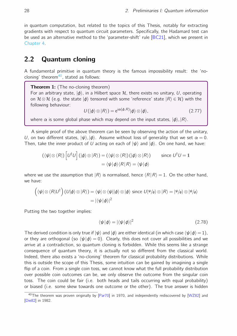
28 2. Preliminaries I: Quantum information
in quantum computation, but related to the topics of this Thesis, notably for extractinggradients with respect to quantum circuit parameters. Specifically, the Hadamard test canbe used as an alternative method to the ‘parameter-shift’ rule [BC21], which we present inChapter 4.
2.2 Quantum cloning
A fundamental primitive in quantum theory is the famous impossibility result: the ‘no-cloning’ theorem40, stated as follows:
Theorem 1: (The no-cloning theorem)For an arbitrary state, |φ〉, in a Hilbert space H, there exists no unitary, U, operatingon H⊗H (e.g. the state |φ〉 tensored with some ‘reference’ state |R〉 ∈ H) with thefollowing behaviour:
U (|φ〉⊗ |R〉) = eiα(φ,R)|φ〉⊗ |φ〉, (2.77)
where α is some global phase which may depend on the input states, |φ〉, |R〉.
A simple proof of the above theorem can be seen by observing the action of the unitary,U, on two different states, |ψ〉, |φ〉. Assume without loss of generality that we set α = 0.Then, take the inner product of U acting on each of |ψ〉 and |φ〉. On one hand, we have:
(〈ψ|⊗ 〈R|)[U†U
](|φ〉⊗ |R〉) = (〈ψ|⊗ 〈R|)(|φ〉⊗ |R〉) since U†U = 1
= 〈ψ |φ〉〈R |R〉= 〈ψ |φ〉
where we use the assumption that |R〉 is normalised, hence 〈R |R〉= 1. On the other hand,we have:(
〈ψ|⊗ 〈R|U†)
(U|φ〉⊗ |R〉) = 〈ψ|⊗ 〈ψ||φ〉⊗ |φ〉 since U|ψ/φ〉⊗ |R〉= |ψ/φ〉⊗ |ψ/φ〉
= |〈ψ |φ〉|2
Putting the two together implies:
〈ψ |φ〉= |〈ψ |φ〉|2 (2.78)
The derived condition is only true if |ψ〉 and |φ〉 are either identical (in which case 〈ψ |φ〉= 1),or they are orthogonal (so 〈ψ |φ〉 = 0). Clearly, this does not cover all possibilities and wearrive at a contradiction, so quantum cloning is forbidden. While this seems like a strangeconsequence of quantum theory, it is actually not so different from the classical world.Indeed, there also exists a ‘no-cloning’ theorem for classical probability distributions. Whilethis is outside the scope of this Thesis, some intuition can be gained by imagining a singleflip of a coin. From a single coin toss, we cannot know what the full probability distributionover possible coin outcomes can be, we only observe the outcome from the singular cointoss. The coin could be fair (i.e. both heads and tails occurring with equal probability)or biased (i.e. some skew towards one outcome or the other). The true answer is hidden
40The theorem was proven originally by [Par70] in 1970, and independently rediscovered by [WZ82] and[Die82] in 1982.

2.2. Quantum cloning 29
from us unless we flip the coin multiple times. Analogously, since quantum theory is ageneralisation of classical probability theory, we cannot know the contents of an arbitraryquantum state with only a single copy of it. Clearly, if we had the ability to clone quantumstates perfectly, a single copy would be sufficient to learn it completely (since we couldmake many clones, and measure in all possible bases to reconstruct the classical descriptionof the state). This impossibility is manifested in the no-cloning theorem.
2.2.1 Beyond the no-cloning theorem
Fortunately (for this Thesis at least), the no-cloning theorem is far from the end of thestory. It turns out there some hidden assumptions in the theorem as presented above.Specifically, we require the ‘cloning machine’ to be perfect41 and deterministic42. Both ofthese assumptions can be relaxed, and doing so has resulted in a rich field of study.
The first work to address these assumptions was [BH96], where the ‘perfectness’ re-quirement was relaxed. Here the idea of approximate cloning was born, meaning that theoutput clones do not have to be exactly the same as the input state, but only somehow‘close’. This closeness is typically measured in terms of the fidelity Eq. (2.69) which werevisit in greater detail in Sec. 2.2.2.1.
The second assumption (determinism) was relaxed originally by [DG97, DG98]. Thisresulted in probabilistic quantum cloning, where the unitary is able to prepare perfect clonesof the input state, but is only able to succeed with a certain probability. Probabilisticquantum cloning is less relevant for this Thesis so we neglect further discussion of it inorder to focus on the approximate version.
2.2.2 Approximate cloning
2.2.2.1 Approximate cloning preliminaries & notation
Even once one has decided to focus on the approximate version of quantum cloning, furthersubdivisions are still possible. To keep track of these, let us begin with some notation.
The three most common properties of quantum cloning machines (QCMs) are:
Universality. Locality. Symmetry.
These properties manifest themselves in the comparison metric which is used to comparethe clones outputted from the QCM, relative to the ideal input states. Almost exclusivelyin the literature, the fidelity (Eq. (2.69)) is the comparison metric of choice, and we revisitthis shortly.
Universality
This refers to the family of states which QCMs are designed for, S ⊆ H (H is the fullHilbert space), as this has a significant effect on their performance. Based on this, QCMs aresubdivided into two categories, universal (UQCM), and state-dependent (SDQCM) quan-tum cloning machines. In the former case all states must be cloned equally well (S =H).
41The output of the cloning unitary must be exactly the same state as the input: |φ〉⊗ |φ〉.42The unitary must be successful with probability one.

30 2. Preliminaries I: Quantum information
In the latter, the cloning machine will be tailored to the family of states fed into it, so S ⊂H.
Locality
Locality refers to whether a QCM optimises a local comparison measure (i.e. check thequality of individual output clones - a one-particle test criterion ([Wer98, SIGA05]) or aglobal one (i.e. check the quality of the global output state from the QCM - an all-particletest criterion).
As in the example above, the state to be cloned, |ψ〉A43, will be inputted into the QCMwith some ‘blank’ state (say |0〉) to carry the clone, plus possibly some ancillary state |R〉to aid with the cloning44. For local cloners, the clones will be the reduced density matricesof the output states from the first two registers:
ρ1 = Tr2R
(U|ψ〉〈ψ |⊗ |0〉〈0 |⊗ |R〉〈R |U†
)ρ2 = Tr1R
(U|ψ〉〈ψ |⊗ |0〉〈0 |⊗ |R〉〈R |U†
) (2.79)
In contrast, for global cloners, we care about the full output state of the QCM, only ne-glecting the ancilla state, |R〉:
ρ1,2 = TrR
(U|ψ〉〈ψ |⊗ |0〉〈0|⊗ |R〉〈R |U†
)(2.80)
Symmetry
Symmetry in a QCM compares one clone relative to the other. Symmetric QCMsrequire each ‘clone’ outputted from the QCM to be the same relative to the comparisonmeasure, which practically means that both clones will have the same local fidelity (seebelow). However, in some scenarios we may wish for asymmetric output for the clones(meaning they have different fidelities). This property obviously only applies to local QCMs.
Next, let us revisit the fidelity as the comparison metric of choice, in the context of thesecriteria. When dealing with local cloners, we define the local fidelity, F jL := FL(ρj ,ρA), j ∈1,2. This compares the ideal input state, ρA := |ψ〉〈ψ |A45, to the output clones, ρj .
In contrast, the global fidelity compares the entire output state of the QCM to a productstate of input copies, FG(ρ1,2,ρA⊗ρA). It may seem at first like the most obvious choiceto study is the local fidelity, however the global fidelity is a relevant quantity for some cryp-tographic protocols. We revisit this explicitly later in the Thesis in Chapter 7.
From one to many
In the above, we only assumed a single state was given, and two clones were required.As a generalisation, we can instead receive M > 1 copies of the input state. In this case, the
43We suggestively use the notation ‘A’, to make the connection to quantum cryptographic protocols laterin this Thesis. In this context, it refers to the mythical ‘Alice’ of Alice & Bob - the canonical protagonists incryptographic protocols. The first reference to Alice and Bob dates back to the seminal RSA paper [RSA78].
44This will behave as an ‘environment’ as in Sec. 2.1.2 in order to implement general quantum operations.45For the purposes of this Thesis, the input state will always be a pure state. A notion of ‘cloning’ can
also be defined for mixed input states, where it is referred to as broadcasting. The no-broadcasting theorem([BCF+96]) generalises the no-cloning theorem in this context.

2.2. Quantum cloning 31
task is to produce N >M output clones46. As such, the input state to the cloning unitaryis (we assume the ancillary register, |R〉, may have an arbitrary dimension):
|ψ〉⊗MA |0〉⊗(N−M)|R〉 (2.81)
This scenario is referred to as M → N cloning ([GM97]), and the standard scenariocorresponds to 1→ 247. Now returning to the symmetry criterion concretely, a symmetricM→ N cloning machine will require:
F jL = F kL , ∀j,k ∈ 1, . . .N. (2.82)
Now that we have our notations in place, let us move onto some concrete examples in thenext section.
2.2.2.2 State-dependent approximate cloning
The earliest result [BH96] in approximate cloning was that a universal symmetric cloningmachine for qubits can be designed to achieve an optimal cloning fidelity of 5/6≈ 0.8333,which is notably higher than trivial copying strategies48 [SIGA05]. In other words, if |ψ〉A isan arbitrary single qubit (pure) state on the Bloch sphere, there exists a UQCM which canachieve the local fidelity FU,j
L,opt = 5/6, j ∈ 1,2. This is not the end of the story however,and much higher fidelities can be achieved using a state-dependent QCM. Roughly speaking,higher cloning fidelities correspond to extra degrees of freedom which are ‘known’ to thecloner. The two most common examples are ‘phase-covariant’ states and ‘fixed-overlap’states, which we describe next.
Phase-Covariant Cloning
Phase-covariant ([BCMDM00]) states are those states which are, roughly speaking,confined to a particular two dimensional plane in the Bloch sphere. The canonical choice isto restrict to the X - Y plane which supports states of the form:
|ψxy (η)〉=1√2
(|0〉+e iη|1〉
)(2.83)
A SDQCM for these states can be constructed ([BCMDM00]) with FPC,jL,opt ≈ 0.85 which
notably is higher than the fidelity achievable with a UQCM.These states are relevant since they are used in BB84 QKD protocols and also in univer-
sal blind quantum computation (UBQC)49 protocols ([BB14, BFK09]). Interestingly, the
46A note on notation: we primarily use m,n in this Thesis to denote the number of qubits, and N,M to betypically a number of samples (as, for example, in Sec. 2.1.7.1) or a vector dimension. In this section, andin Chapter 7, we switch to M,N indicating the number of qubits, for historical consistence.
47It is interesting to note that in the limit M →∞, an optimal cloning machine becomes equivalent to aquantum state estimation machine [SIGA05] for universal cloning.
48Examples of trivial cloning machines are where one simply measures the state, and prepares two copiesaccording to the measurement result, or so-called trivial amplification where one simply prepares a randomstate as the second clone, and the first is allowed to pass through undisturbed. These trivial strategies canachieve an average fidelity of 75% ([SIGA05]), so the reader should keep this number in mind, particularly inChapter 7.
49Similar acronyms become confusing.

32 2. Preliminaries I: Quantum information
cloning of phase-covariant states can be accomplished in an economical manner, meaningwithout needing an ancilla register, |R〉 ([NG99]). However, as noted in [SG01, SIGA05],removing the ancilla has consequences for quantum cryptography and protocol attacks,which we revisit later in this Thesis.
An alternative parameterisation of phase-covariant states are those in the X - Z plane:
|ψxz(θ)〉= cos(θ)|0〉+ sin(θ)|1〉 (2.84)
The optimal cloning fidelity here is the same as with the states (Eq. (2.83)), since in bothcases, one degree of freedom is revealed.
To round off this discussion, let us present an explicit quantum circuit which implementsthe above cloning transformations. A unified circuit ([BBHB97, FWJ+14, FMWW01]) forall above cases (universal, X-Y and X-Z phase-covariant cloning) can be seen in Fig. 2.4.The parameters of the circuit, α = α1,α2,α3, are chosen depending on the family ofstates to be cloned ([BBHB97, FMWW01, FWJ+14]).
Explicitly, we have suitable angles for universal cloning:
αU1 = αU3 =π
8, αU2 =−arcsin
√(1
2−√
2
3
)(2.85)
whereas for phase-covariant cloning of X-Y states, we require:
αxy1 = αxy3 = arcsin
√(1
2−
1
2√
3
)≈ 0.477,
αxy2 =−arcsin
√(1
2−√
3
4
)≈−0.261 (2.86)
Figure 2.4: Ideal cloning circuit for universal and phase-covariant cloning. The Preparation circuit preparesthe registers to receive the cloned states, while the Cloning circuit transfers information. Notice, the outputregisters which contain the two clones of |ψ〉A are the last and penultimate registers, while the ancilla, Rappears at the first register.
2.2.3 Cloning of fixed overlap states
An alternative family of well known states are those which are not defined by their inhabi-tancy of a particular plane of the Bloch sphere, but instead by their overlap. In this case,

2.2. Quantum cloning 33
we usually care about only a finite set of states50. For our purposes, we usually assume wehave only two51 states in this set, typically parametrised as follows:
|ψ1〉= cosφ|0〉+ sinφ|1〉|ψ2〉= sinφ|0〉+ cosφ|1〉
(2.87)
which have a fixed overlap, s := 〈ψ1 |ψ2〉 = sin2φ. We refer to this set of states as fixed-overlap states52. Interestingly fixed-overlap cloning was one of the original scenarios studiedin the realm of approximate cloning [BDE+98], but was difficult to tackle analytically sowas somewhat sidelined. Furthermore, fixed-overlap cloning has been used to demonstrateadvantage related to quantum contextuality [LS20b].
Let us now turn to the optimal achievable cloning fidelities for these states. It was shownearly on ([BDE+98]) that the optimal local cloning fidelity for 1→ 2 cloning53 is given by:
F FO,jL,opt =
1
2+
√2
32s(1 + s)
(3−3s+
√1−2s+ 9s2
)×√−1 + 2s+ 3s2 + (1− s)
√1−2s+ 9s2, j ∈ 1,2 (2.88)
It can be shown that the minimum value for this expression is achieved when s = 12 and
gives F FO,jL,opt≈ 0.987, which is much better than the symmetric phase-covariant cloner (recall
FPC,jL,opt ≈ 0.85.To complement this, optimal global fidelity of cloning the two states in Eq. (2.87) is
given by:
F FOG,opt(M,N) =
1
2
(1 + sM+N +
√1− s2M
√1− s2N
)(2.89)
At this point, it is necessary to draw attention to a certain fact which we will encounter ingreat detail later in this Thesis. Namely, it can be shown that the SDQCM which achievesthis optimal global fidelity, does not actually saturate the optimal local fidelity (i.e. theindividual clones do not have a fidelity given by Eq. (2.88)). Instead, if we take the QCMwhich achieves an optimal value of Eq. (2.89), and compute what the local fidelity of eachclone would be, we get [BDE+98]:
F FO,jL,∗ (M,N) =
1
4
(1 + sM
1 + sN
[1 + s2 + 2sN
]+
1− sM
1− sN[
1 + s2−2sN]
+ 21− s2M
1− s2N
[1− s2
])(2.90)
which (taking M = 1,N = 2) is actually a lower bound for the optimal local fidelity, F FO,jL,opt
in Eq. (2.88). As such, optimising either the local or global fidelities to find the optimalvalues will lead to different answers, in general54. We return to this issue in Chapter 7.
50As opposed to phase-covariant states, which have a continuous parameterisation.51We can also consider this type of cloning with four input states instead, which are usually the two given
in Eq. (2.87) plus their orthogonal counterparts. We use both examples in Chapter 7 of this Thesis.52Confusingly, cloning states with this property is historically referred to as ‘state-dependent’, but as we
discussed above state-dependent cloning is a more general scenario where the cloner generically depends onthe input state properties.
53This messy expression gives hints for the tricky analytical nature of this problem, even in the simplestscenario.
54This is not always the case however, for universal and phase-covariant cloning, local and global optimisationare equivalent.


3
Preliminaries II: machine learning
3.1 Machine learning
“Machine intelligence is the last invention that humanity will ever need to make.”– Nick Bostrom, TED, 2015
Having introduced most of the prerequisites in quantum computation, it is time toturn our attention to second pillar of this Thesis, the expansive field of machine learning(ML). There are many ways of describing what this field is, and what it aims to do, butroughly speaking, machine learning is an arm of artificial intelligence (AI) which aims totrain machines to learn to solve some problem. Most commonly, they (computers) learnfrom data and solve problems without being explicitly programmed to do so. As such, thealgorithms developed by machine learning practitioners are usually data-driven, and in manycases, their success is dependent on the quality of data available to them. The methodsand techniques used in ML algorithms draw heavily on the field of statistics and the type ofmachine learning we use here can also be referred to as statistical learning. For an excellentand gentle introduction to this topic, see [JWHT13a].
Machine learning algorithms are canonically split into three main categories1:
Supervisedlearning.
Unsupervisedlearning.
Reinforcementlearning.
Each of these subfields are large, and we do not attempt to provide a comprehensiveoverview here. In this immediate section, we are also only referring to classical tasks, i.e.those where the underlying data is classical (vectors, matrices, etc.). We generalise thiswhen discussing quantum machine learning in Chapter 4.
The typical differences between these learning types is that supervised learning learnswith labels (we give a more precise definition in Sec. 3.3.1), unsupervised learning learnswithout labels, and reinforcement learning learns from experience or via interaction. Toavoid unnecessary tangents, we focus in this Thesis on the two particular examples whichwe use explicitly, one from supervised learning, and the other from unsupervised learning.We also take the viewpoint that (un)supervised learning is learning with(out) access to thecorrect answer (or more technically, the ‘ground truth’) for given problem instances, rather
1Although, by modern standards, these categories are oversimplified. For example, there exists a plethoraof intermediate categories, and merging of the ideas in each one. A major example is semi-supervised learning.
35

36 3. Preliminaries II: Machine learning
than with(out) labels. The reason is that with this modification, the definitions also thenencompass the contents of Chapter 7 of this Thesis.
However, for now, let us focus on the two following (classical) tasks:
1. Classification (Supervised learning).
2. Generative modelling (Unsupervised learning).
Before diving into these applications, let us first introduce some terminology. Firstly, wehave a machine learning model. A model may be deterministic or probabilistic, and may besupervised or unsupervised in nature. In the supervised setting, a model is usually a proxyto represent a function, f (x), defined on some space x ∈ X . A generative model, on theother hand, is a proxy for a probability distribution, p. One of the most widespread classicalmachine learning models are neural networks, which we discuss in Sec. 3.2 which can beused to solve both of the problems above. At the time of writing, the closest2 counterpart inthe quantum realm to a neural network is the parametrised quantum circuit (PQC), whichwe introduce in Sec. 4.1. These models usually belong to a model family,M; for examplea family of functions, M := F := f or probability distributions, M := D := p3. It isalso common to parametrise the model family, M→Mθ. A machine learning algorithmthen optimises these parameters in order to learn, which corresponds to finding the optimalcandidate in the model family to solve the problem of interest. As we use neural networks asour benchmarkmodel, we view gradient descent as our canonical machine learning algorithm,since we use it almost exclusively in this Thesis.
The parameters, θ, define the model, but there is another type of parameter which onemust also be concerned with. These are hyperparameters, which we define as follows:
Definition 12 (Hyperparameters).In a machine learning algorithm, a hyperparameter is a parameter used to control thelearning procedure. It is distinct from a model parameter in that it is ‘outside’ themodel, and usually associated to the learning algorithm itself.
Next, we have the concept of (labelled) data.
Definition 13 (A dataset).A dataset is a collection of datapoints, x ii , from some input domain, X . Eachelement of a labelled dataset will also have a corresponding label, y i , coming fromsome domain, Y, for each datapoint, x i . We may also have a probability distribution,D ∈ D defined over X , so x i ∼D.
The above definition of data is intentionally flexible, as in general datapoints may bebinary, real or complex-valued scalars (x i ∈ 0,1/R/C), vectors (x i := z i = [z1, . . .zn]T ∈Rn/Cn) or even quantum states in a Hilbert space, x i := ρi ∈ H. In this Thesis, data willtake the form of each of the above. Generally speaking, the difference between supervisedand unsupervised learning is the access to, or lack of, the labels, y i .
2We use the term ‘closest’ here lightly - there is still discussion in the community about what shouldbe considered the quantum analogue of a neural network. For a (now outdated) discussion of this topic,see [SSP14].
3This is actually slightly misleading since supervised learning problems also are defined with a distributionover the input domain.
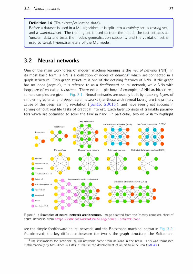
3.2. Neural networks 37
Definition 14 (Train/test/validation data).Before a dataset is used in a ML algorithm, it is split into a training set, a testing set,and a validation set. The training set is used to train the model, the test set acts as‘unseen’ data and tests the models generalisation capability and the validation set isused to tweak hyperparameters of the ML model.
3.2 Neural networks
One of the main workhorses of modern machine learning is the neural network (NN). Inits most basic form, a NN is a collection of nodes of neurons4 which are connected in agraph structure. This graph structure is one of the defining features of NNs. If the graphhas no loops (acyclic), it is referred to as a feedforward neural network, while NNs withloops are often called recurrent. There exists a plethora of examples of NN architectures,some examples are given in Fig. 3.1. Neural networks are usually built by stacking layers ofsimpler ingredients, and deep neural networks (i.e. those with several layers) are the primarycause of the deep learning revolution ([Sch15, GBC16]), and have seen great success insolving difficult real life tasks of practical interest. Each layer consists of trainable parame-ters which are optimised to solve the task in hand. In particular, two we wish to highlight
Figure 3.1: Examples of neural network architectures. Image adapted from the ‘mostly complete chart ofneural networks’ from https://www.asimovinstitute.org/neural-network-zoo/.
are the simple feedforward neural network, and the Boltzmann machine, shown in Fig. 3.2.As observed, the key difference between the two is the graph structure; the Boltzmann
4The inspirations for ‘artificial’ neural networks came from neurons in the brain. This was formalisedmathematically by McCulloch & Pitts in 1943 in the development of an artificial neuron ([MP43]).

38 3. Preliminaries II: Machine learning
machine contains loops whilst the feedforward network is acyclic. The parameters in bothmodels consist of trainable weights, W , and biases, b (or self-loops). We focus on thesetwo examples, because they are canonical examples of classical models for the two primary(classical) ML tasks in which we are interested in this Thesis. Specifically, the feedforwardnetwork is used for classification tasks, and the Boltzmann machine is used for generativemodelling of probability distributions. We explicitly use the Boltzmann machine in Chapter 6.
Figure 3.2: Two canonical neural networks (NN). (a) A feedforward NN with an input, hidden and outputlayer. (b) a fully connected Boltzmann machine with visible (blue) and hidden (green) units.
3.2.1 Feedforward neural networks
Let us begin with the feedforward NN. This consists of an ‘input’ layer, into which the datais inserted, a ‘hidden’ layer which increases the representational power of the model, anda final output layer. These layers are connected by the weights, which form a matrix. Forexample, in Fig. 3.2(a), W13 is the weight connecting vertices v1 in the input layer andv3 in the hidden layer. Putting these weights together forms the matrix W IH. Each nodein Fig. 3.2(a) may also have its own bias, b. These weights and biases are the trainableparameters of the network, θ = W IH,WHO,bI,bH. Given an input data vector, x , theoutput of this network is given by:
fθ(x) := yout(x) := σ(WHOy1(x) +bH)
y1(x) := σ(W IHx +bI)(3.1)
The output vector can be a vector of probabilities, for example (as we shall see in Sec. 3.3.1)the probabilities that the input sample belongs to each of the desired classes. The function,σ, is crucially important in a neural network as it provides a non-linearity to the model5,
5Without this non-linear function after each layer in deep neural networks, the model would be entirelylinear, and a deep network would be equivalent to a single layer model. Implementing such a non-linearity todesign quantum neural networks is an active area of research, and is problematic due to the naturally linearnature of quantum mechanics.

3.3. Machine learning tasks 39
called an activation6 function. Common choices for σ are the sigmoid, tanh or the ReLU(recitified linear unit) activation functions:
σsigmoid(x) =1
1 +e−xσtanh(x) = tanh(x) σReLU(x) = max0,x (3.2)
These functions provide differentiable alternatives to the more obvious binary step functionwhich could be used as an activation function.
3.2.2 The Boltzmann machine
The Boltzmann machine is an example of a physics inspired model known as an energybased model. This means it is completely defined by an energy function, which in the caseof the Boltzmann machine is given as an Ising model:
E(z) :=−
(∑i<j
Wi jzizj +∑k
bkzk
)(3.3)
The variables zi ∈ +1,−17 are the values that the nodes, vi in Fig. 3.2(b) can take.Each configuration of the spins will have its associated energy, and the model is definedby the distribution over these energy values. In other words, the probability of a givenenergy (a given configuration of the n variables, z = [z1, . . . ,zn]T ) is given by the Boltzmanndistribution:
pθ(z) :=eE(z)
Z , (3.4)
where Z := ∑z eE(z) is the partition function, a normalisation constant which is intractableto compute in general, due to the exponentially many terms in the sum over 2n possibleconfigurations of z . We use the notation, zi , to denote a specific realisation of the value ofnode i and we use vi to label the node itself. As observed in Fig. 3.2(b), some of the nodes inthe Boltzmann machine may be hidden also8 which are used to increase the representationalpower of the model, and as such the data is associated only to the remaining ‘visible’ nodes.In Sec. 3.3.2, we will see how the Boltzmann machine can be used for the second of ourtasks: generative modelling. In this context, the parameters, θ= Wi j ,bk of the Boltzmannmachine will be used to fit the probability distribution of the model to a data distribution.
3.3 Machine learning tasks
3.3.1 Classification as supervised learning
As mentioned above, we will use classification as the primary example of supervised learning.Before diving into the special case, let us define the general problem in this domain [SP18].
6Coming from the ‘activation’ of a biological neuron when sufficient input signal is applied.7This is inherited from the notation of atomic spins in the Ising model of ferromagnetism, named after
Ernst Ising. It is sometimes convenient to associate these variables to be 0 or 1 instead. The weights betweennodes Wi j are also called ‘interaction’ terms, and denoted Ji j , and the biases, bk , are called local (external)magnetic field strengths and denoted hk for historic reasons.
8Hidden nodes are one feature which generalise the Boltzmann machine from its simpler counterpart, theHopfield network, named after John Hopfield for his 1982 paper [Hop82]. The Hopfield network is also adeterministic model.

40 3. Preliminaries II: Machine learning
Definition 15 (Supervised learning problem).Given an input domain, X , and an output domain, Y, a training data set:
D = (x1,y1), . . . ,(xM ,yM) (3.5)
of training pairs, (xm,ym) ∈ X ×Y with m = 1, . . . ,M of training inputs, xm andtarget outputs ym as well as a new unclassified input, x∗ ∈ X , guess or predict thecorresponding output y∗ ∈ Y.
Two of the most common examples of supervised learning problems are regression andclassification. Roughly speaking, the difference is in the nature of the variables or labels, yi .In regression problems, the labels are continuous (or quantitative), whereas in classification,the labels are discrete (meaning categorical or qualitative) ([JWHT13b]). There are aplethora of methods to solve these problems, and in this thesis we use a quantum computerto do so (for the classification version)
The most basic form of classification is binary classification, where the labels are only twopossible values i.e. y i ∈ 0,1, so each data point, x i , is assigned a value of 0 or 1. The goalof the ‘classifier’ is to learn this function, f , mapping the data to their corresponding labels.This function may come from a particular function family, F , which defines our model class.As discussed at the start of this section, we can parametrise this function family, f → fθ. Ifwe use a feedforward neural network for this task the parameters correspond to the weightsand biases of the network. In Sec. 3.6 we will introduce a slightly more formal discussionfor completeness.
A very common baseline example (in the classical world) of such a classification task isthe classification of digits, using the famous MNIST database, which consists of 60,000
training images and 10,000 test images of handwritten digits from 0 to 9. The goal is tolearn the mapping from image to digit label, so to classify all images in the test set correctly.
Training machine learning models has become very accessible in recent years with the de-velopment of deep learning software, particularly in Python, such as TensorFlow [ABC+16],Pytorch [PGM+19] and Keras [Co15]. Using Tensorflow, we can very easily load the aboveMNIST dataset, and train a feedforward NN (as in Fig. 3.2(a)) to classify images. Fig. 3.3shows the results of 15 digits from the trained model. Under each image, we see whatthe model labelled the test digit as, and the corresponding probability of doing so. Theparticular trained model had 100% confidence about each image, except the digit 5 in thefirst row and third column, which has a 4% chance of being the digit 6, according to themodel. From this example, one can imagine how neural networks have become so powerful,and widely used - modern architectures can have billions of parameters [TGR15] and areapplied on much more challenging tasks than digit recognition. As quantum computersscale in size, we hope they will be able to tackle similar problems.
3.3.2 Generative modelling as unsupervised learning
Chapter 6 of this Thesis will be focused on using quantum computers for generative mod-elling, which as mentioned is our primary example of unsupervised learning.
Unlike the supervised learning models discussed in the previous section, generative modelscan be significantly more complex, since they have the ability to also generate new dataobservations, sometimes called ‘synthetic data generation’. While the former deals with

3.4. Training a neural network 41
596%(5) 0123456789
6100%(6) 0123456789
1100%(1) 0123456789
01234567890100%(0)
01234567894100%(4)
01234567899100%(9)
9100%(9) 0123456789
01234567897100%(7)
0100%(0) 0123456789
0100%(0) 0123456789
9100%(9) 0123456789
4100%(4) 01234567892100%(2) 0123456789
01234567891100%(1)
1100%(1) 0123456789
Figure 3.3: A feedforward neural network trained on the MNIST training dataset, classifying exampleimages in the test dataset. The boxes to the right of each digit show the probability assigned to each possiblelabel. We see all of these digits were correctly labelled, since the trained model assigns a high probabilityweight to the correct label. The model in question is a simple neural network consisting of an input layer, ahidden layer with 128 nodes, and a final output layer with 10 nodes, where each node in the output representsa digit, 0, . . . ,9. This figure was produced using an example tutorial in Tensorflow [ABC+16].
parametrised functions, generative models use parametrised probability distributions, pθ,which again come from some distribution model family, D. The distribution, pθ may becontinuous, in which case pθ is the probability density function (PDF) over the samplespace, X . In this Thesis however, we exclusively use discrete distributions over X , so pθ isa probability mass function (PMF). In particular, we will take X = 0,1n.
In the generative modelling problem, we are required to learn some ‘data’ distribution,which we denote π over some space Y. We may be given direct access to the probabilities,π(y),y ∈Y, but more commonly we will only have a dataset ofM vectors sampled accordingto π, y iMi=1,y ∼ π. We further assume π is a discrete distribution over 0,1n, so forefficiency we only have M = O (poly(n)) samples. Given our model, pθ, the goal is thento fit pθ to π, using the parameters, θ. If we were to use a Boltzmann machine for thistask, we would fit the weights and biases in the energy function Eq. (3.3) and train themodel distribution, pθ(z). In Fig. 3.4, we demonstrate generated results using a restrictedBoltzmann machine on the same MNIST dataset as in Fig. 3.3. In the next section, weprovide some further detail on how to train such neural network models. This will beespecially relevant for the contents of this Thesis, since the methods we use to train ourquantum models incorporate these exact same techniques (with suitable modifications).
3.4 Training a neural network
There are a multitude of methods to train machine learning models, such as the neuralnetworks we presented in the previous section. For particular models and algorithms, suchas the support vector machine (SVM) the training procedure is a (relatively) simple convexoptimisation problem, provided one can easily compute the underlying kernel matrix (e.g.the one defined in Theorem 2 in Sec. 2.1.7.1). Unfortunately, for neural networks, theproblem is not so simple. This is because the loss or cost9 function landscape may becomehighly non-convex due the choice of our parameterisation, θ. In Sec. 7.2.1 we will discuss
9We use these terms interchangeably here; some may consider the cost function to be the loss function,but with the addition of regularisation.

42 3. Preliminaries II: Machine learning
Figure 3.4: A restricted Boltzmann machine learning to generate MNIST digits. From left to right, wesee improving performance (in terms of resolution), indicating that the model is learning to generate digitswhich look similar to those in the test set (the rightmost image). In the RBM, every (visible) spin can by usedto represent each pixel being black or white (up or down).
desirable properties of cost functions in more detail, since they apply to both quantum andclassical machine learning models. For now, let us simply assume that a cost function issome function of our model parameters, C(θ), and that it gives us a method to measurehow well we are doing in the training process. The goal of training is to minimise10 C(θ),i.e. solve θ∗ = argminθC(θ). In many common examples, the cost can be defined as anexpectation over the dataset which, in the limit M→∞, approaches the expectation overthe full distribution from which each datapoint is drawn, x i ∼D:
C(θ) = Ex∼DCx(θ)≈1
M
M
∑i=1
Ci(θ)︸ ︷︷ ︸Remp
(3.6)
Ci(θ) is the term evaluated using a single sample from the dataset, x i , and Remp is knownas the empirical risk. Minimising this quantity is known as empirical risk minimisation, andis commonly used as a proxy to minimise our true objective, C.
The cost function defines the cost landscape as a function of θ, and the training pro-cedure is to find the absolute (global) minimum of C(θ). However, as we mentioned, thisproblem is non-convex, meaning many sub-optimal local minima exist and may also befound. The goal of a training algorithm is usually to efficiently traverse this landscape tofind the global minimum.
Let us now focus on NNs specifically. Methods to train NNs can be roughly split into twocategories - gradient-free and gradient-based. Gradient-free methods are also called zeroth-order methods, since they optimise C using only information about C itself. A non-exhaustivelist of gradient-free optimisation methods include Bayesian optimisation ([Moc89]), evo-lutionary methods ([BS02]) or simulated annealing ([LA87, KGV83]), see [RS13] for anoverview. Gradient-free methods are useful in cases where perhaps the gradients of C arenot available, or difficult to compute.
In cases where we can compute gradients, we can use alternatively gradient-based opti-misation. As the name suggests, these methods use first-order gradient methods to optimise
10We can assume this WLOG since if one may want to maximise C(θ), we can convert to a minimisationproblem by defining Cθ =−Cθ and minimising Cθ.

3.4. Training a neural network 43
C. One may also consider training algorithms which use second-order gradient methods re-quire evaluation of also the Jacobian or Hessian of C. For this Thesis, first-order gradientbased methods will suffice.
The main algorithm we use is stochastic gradient-descent (SGD):
Definition 16 (Stochastic gradient descent).Given a single sample from a dataset, x i , stochastic gradient descent updates theparameters, θ, as:
θ(j+1)← θ(j)−∆C(η, j,θ) = θ(j)−η∇θCi(θ) (3.7)
where j defines an epoch, η is a learning rate and ∇θ denotes the gradient vectorwith respect to each parameter, θk .
The number of epochs is typically a predefined number, and one epoch constitutes onecomplete pass over the training data. The learning rate, η, controls the speed of trainingand both of these are hyperparameters (see Definition 12) of the learning algorithm. WhileSGD is very fast, it may suffer from high variance since only a single training sample isused to estimate the true gradient. Instead, one can consider mini-batch gradient descent,where a certain number of samples are taken (given by a batch size, b) from the trainingdataset to estimate ∇θC(θ) for each update. Taking the batch size to be the same asthe training data set size (b = 1) recovers SGD as in Definition 16, while taking b = M
recovers ‘regular’ gradient descent, where the entire dataset is used in each parameterupdate. Clearly, choosing the batch size also heavily affects the speed of training, and so itis another hyperparameter.
Notice that we have written the ‘update rule’ for SGD in Eq. (3.7) in two different ways,one including a term ∆C(η, j,θ), and then a specification of this expression which is thatused specifically for SGD, i.e. an update using a term η∇θCi(θ). The former expression iswritten in this form to allow more general update rules. For example, one may consider thatthe update depends on the epoch, j , i.e. time dependence, or a more complicated expressionin terms of the parameters, θ.
In this Thesis, we primarily use an update rule known as Adam, which uses an adaptivelearning rate, η, and incorporates the notion of momentum to SGD.
Definition 17 (Adam update rule ([KB15])).The adaptive momentum estimation (Adam) update rule to the parameters is givenby the following:
θ(j+1)← θ(j)−∆AdamC(η, j,θ) = θ(j)−ηinit√v j +ε
mj , (3.8)
mj =mj
1−βj1, v j =
v j
1−βj2, (3.9)
mj = β1mj−1 + (1−β1)∇θ(j) C(θ), (3.10)
v j = β1v j−1 + (1−β2)[∇θ(j) C(θ)]2 (3.11)
where β1,β2,ε,ηinit are hyperparameters. βk1 ,k ∈ 1,2 means βk raised to the powerj , which results in a exponential decay.
44 3. Preliminaries II: Machine learning
The hyperparameters, β1,β211, are heavily weighted towards a value of 1, which means
that random fluctuations in the gradient, if they are sufficient small, will contribute less thanthe weighted sum of previous gradients. Therefore, the optimisation is likely to keep movingin the same direction at each epoch (hence the term ‘momentum’). The vector, v , keepstrack of the second moment of the gradient, and the terms mj , v j are computed in order tocorrect the tendency of mj ,v j to be biased towards the zero vector, 0, since they are bothinitialised at 0. One could also choose alternative update rules such as Adagrad [DHS11],Adadelta [Zei12], NAdam [Doz16] or a plethora of others. In many cases, the update ruleis designed to encourage large values at the start of training, but decrease towards the endso we do not overshoot the minimum we are after. As we shall see in Sec. 4.1, for trainingmodern quantum machine learning models, one may wish to include quantum awareness intosuch optimisers. To this end, versions of update rules have been proposed by incorporatingquantum measurement error [KACC20], or to partially overcome linear scaling of computingquantum gradients [CMMS20, GZCW21] (see Eq. (4.13) in Sec. 4.1.3). We will not useany of these more complicated methods in this Thesis, so we will not discuss them furtherhere. However, we remark that all of these methods could be applied and tested on eachof the applications we study in the subsequent chapters.
3.4.1 Computing gradients
Finally, let us remark on the computation of the gradient terms, ∇θC(θ) for the two classicalmodels we have introduced above. For the feedforward NN, we do this to illustrate adifference between the quantum models we discuss in Sec. 4.1 and for the Boltzmannmachine, we explicitly use it later in this Thesis in Chapter 6.
3.4.1.1 Feedforward neural networks
For training feedforward neural networks, a key breakthrough was the discovery of thebackpropagation algorithm ([RM87]), which is short for the backpropagation of errors inthe neural network. Recall the structure of the simple example feedforward NN in Fig. 3.2.We ultimately want to compute the gradient with respect to each parameter, the weights,WHO,WIH plus the biases of each node, bI,bH. Fortunately, the output vector, yout is aconcatenation of simple functions applied to the input. So the gradient can be computedusing the simple chain rule (take for example the gradient with respect to the input biasvector, bI with a slight abuse of notation):
∂C(W,b)
∂bI=∂C(W,b)
∂yout×∂yout
∂y1×∂y1
∂bI(3.12)
=∂C(W,b)
∂yout×∂σ(WHOy1 +bH)
∂y1×∂σ(W IHx +bI)
∂bI(3.13)
If we use a sigmoidal activation function, y(z) := σsigmoid(z) = 1/(
1 +e−z), the derivative
is simple: ∂σsigmoid(z)/∂z = σsigmoid(z)(1−σsigmoid(z)). Furthermore, since each layer beforethe activation function has a simple affine form, it can also be trivially computed. We must
11The original Adam paper chooses β1 = 0.9, β2 = 0.999, ε = 1× 10⁻⁸, which are the values we usethroughout this Thesis.

3.4. Training a neural network 45
also obviously assume that the cost function is a differentiable function with respect to yout,but one can choose the `2 norm, Eq. (2.47) as a simple example.
One crucial feature of the above derivation is the computational efficiency of the cal-culation. By staring at Eq. (3.13) and beginning with the parameters at the end or thenetwork, one can see how each gradient evaluation reuses the same computational steps.For example, to compute the gradient with respect to every weight and bias, we must be-gin by computing ∂C(W,b)/∂yout. Similarly, the computation of every parameter gradient willrequire an evaluation of a gradient for the layer immediately after it. Storing these inter-mediate computations as one trains the network, rather than re-computing them for eachparameter separately, massively improves the complexity. This general principle underpinsthe field of differentiable programming, and automatic differentiation. Most deep learninglibraries such as Tensorflow and PyTorch contain an autodiff function which can performthis differentiation automatically for many functions. We highlight this here to make theconnection to the quantum case. We shall see in Sec. 4.1.3 how the ‘parameter-shift’ rule,and the black box nature of quantum computers prohibits these chain rule type of gradientcomputations (at least in the near term). As such, for training quantum models we must paythe price of a linear scaling in the number of parameters which may be a major bottleneckas problem sizes scale. We will revisit this discussion in Sec. 4.1.3.
3.4.1.2 Boltzmann machine
Now, let’s turn to the training of the Boltzmann machine. Recall that here we are tryingto match the visible variables of the network (see Fig. 3.2) to a data distribution π, givensome M samples from π,y iMi=1,y i ∼ π(y). As with training a feedforward neural network,we require a cost function, C(θ), to indicate how well our model is training. Contrary tothe previous example, now we must use cost functions which deal with probability distri-butions, rather than vectors or labels. Here is where the probability metrics we introducedin Sec. 2.1.7.1 will become useful. For training Boltzmann machines, we use the KL diver-gence Eq. (2.49), as this is one of the most common cost functions. Specifically, if werecall the definition of the KL divergence between the Boltzmann distribution, pθ(v) andthe data, π in terms of the cross entropy:
KL(π,pθ) = ∑x
π(x) logπ(x)−∑x
π(x) logpθ(x) (3.14)
Now the first term is the entropy of the data distribution, which does not depend on ourmodel parameters, hence we ignore it in the optimisation problem. As such, our costfunction then can be defined as:
C(θ) :=−∑x
π(x) logpθ(x)≈−1
M
M
∑i=1
logpθ(y i) (3.15)
which is the empirical negative log-likelihood. Minimising this expression, maximises the‘likelihood’ that the training data vectors, y i are observed from our model distribution.Now, in this case, our trainable parameters are the weights and self-loops in the Boltzmannmachine graph (Fig. 3.2(b)). Due to the relatively simple form of the probability distributiongenerated by a Boltzmann machine Eq. (3.3), Eq. (3.4), we can compute the derivativeswith respect to an edge of the graph as (the edge i j connecting nodes i and j):
∂C(θ)
∂Wi j= 〈v iv j〉π−〈v iv j〉pθ ,
∂C(θ)
∂Wk= 〈v k〉π−〈v k〉pθ (3.16)

46 3. Preliminaries II: Machine learning
which essentially matches the expectation value of each node 〈v k〉 and the correlationsbetween pairs of nodes, 〈v iv j〉 between the model and data distributions. One might expectthat with these expressions, the training is straightforward. Unfortunately, it is not sosimple. In order to evaluate Eq. (3.16), we need to be able to efficiently sample fromour model distribution, pθ. A fully connected Boltzmann machine is not trivial to samplefrom, unfortunately. In order to bypass this problem, practitioners commonly restrict theconnectivity to define restricted Boltzmann machines (RBMs), which are defined with onlya bipartite graph between visible and hidden nodes rather than a fully connected one. Anexample of an RBM is given in Fig. 3.5.
Figure 3.5: An example 6 visible node restricted Boltzmann machine. The RBM has hidden nodes and 12
parameters overall. For this illustration, we assume the weights between nodes, Wi j , are not trainable. Biasesfor visible and hidden nodes, bvi ,bhi correspond to the self-loop weights in Fig. 3.2(b). We shall explicitly usethis RBM structure in Chapter 6.
For an RBM, there exists an algorithm to generate samples from pθ, which is calledk-step contrastive divergence [Hin02, CPH05, Hin12]. A Gibbs sampler is an algorithmused to prepare a sample on the visible units as the end result of a Markov chain MonteCarlo (MCMC)12 algorithm. Due to the bipartite nature of the RBM graph, the visible andhidden nodes are conditionally independent given each other. This means that all the nodesin each layer can be updated simultaneously, which significantly improves the time requiredto generate a sample. In contrast, a fully connected Boltzmann machine would require eachnode to be considered separately in the Gibbs sampling process. Running a Markov chain foran infinite number of steps would generate an exact sample from the desired distribution,however k-step contrastive divergence halts after k steps of the chain, and produces andapproximate sample. Hinton in his original work [Hin02] observed that taking simply k = 1
was sufficient to generate good samples from the RBM. This k = 1 contrastive divergencewas the method used to generate samples from, and train, the RBM in Fig. 3.413. We havediscussed the above method to generate samples from the RBM for completeness, howeverwe shall not actually use it directly in this Thesis. Instead, we use an alternative methodbased on path-integral Monte Carlo (PIMC)14, which we revisit in Chapter 6.
12A Markov chain MC algorithms are a family of probabilistic algorithms which enable sampling from adesired distribution which is constructed as the equilibrium distribution of a Markov chain. A Gibbs sampler isa special case which requires the conditional distributions of the target to be exactly samplable, since theseare used to update the elements of the sample.
13This implementation uses code adapted from https://github.com/meownoid/tensorflow-rbm, whichalso adds a momentum term to the gradient update (see ∆C in Eq. (3.8)).
14In contrast to Markov chain Monte Carlo, the path-integral version computes a statistical estimate of afunction using the path-integral formulation of quantum mechanics.

3.5. Kernel methods 47
3.5 Kernel methods
In Sec. 2.1.7.1 we briefly introduced feature maps and kernels, in terms of the mathematicalmachinery required to use them in probability distance measures. Let us now revisit kernelmethods in their appropriate context and use in machine learning more generally. We thendiscuss the extension of kernel methods to the quantum world in Sec. 4.2.
Previously, we presented a feature maps and kernels as being simply functions, and theirinner products respectively. In reality, the definition of kernels and their relationship tofeatures maps is more of a subtle point which we address in the following section. Webuild to these discussions by working through an example in machine learning where themotivation to use kernels becomes apparent. The example we choose to illustrate thisis the canonical support vector machine (SVM), which was one of the most favourableclassification algorithms before the advent of deep learning. Let us first introduce the basicsof the SVM before discussing how kernels fit into the picture. The most basic version isthe linear SVM. Here, we have a labelled dataset (x i ,y i),x i ∈ X ,y i ∈ +1,−1Mi=1, andthe linear SVM classifies points by fitting a maximum margin15 hyperplane (a straight line)in the sample space, X . The line parameters are a weight vector and a bias, w ,b withthe hyperplane defined as wT x − b = 0. This line must be constructed such that everypoint labelled yi = 1 has wT x−b> 1 and those labelled yi =−1 have wT x−b6−1 whereequality defines the parallel hyperplanes to the original line and describe the margin. Now, inorder to actually find the maximum margin hyperplane in the SVM, one solves the followingoptimisation problem:
w∗ =min ||w ||2 (3.17)
subject to y i(wT x i −b)> 1 (3.18)
where the condition in Eq. (3.18) ensures that the predictions of the SVM (given byy i = sgn
(wT x i −b
)), match the true labels, y i .
Of course, a linear SVM will only work16 if the data is linearly separable in the originalspace, X , which will not be the case in many scenarios. To remedy this, the ‘non-linear ’ SVMdoes not fit a hyperplane, but instead maps points x i ∈X to the ‘feature’ space, H. We canthen solve a similar optimisation problem to Eq. (3.17) but replacing the original vectorswith their feature mapped versions, φ(x i). As a result, the decision boundary generatedin H will be still linear, but when mapped back into X , will become non-linear, due to thenon-linearity of φ.
However, we have not yet mentioned how the kernels (the inner products of the featurevectors) fit into this picture. The answer lies in the dual formulation of the optimisationproblem Eq. (3.17). In the original linear SVM, this dual contains terms involving only innerproducts of the datapoints, (x i)T x j . Therefore, when replacing x i with their correspondingfeature maps, φ(x i), and deriving the non-linear version of the dual problem, we get innerproducts of the feature vectors, φ(x i)Tφ(x j) i.e. kernels17. This is referred to as the ‘kernel
15The margin is the area between the fitted line, and the closest data points, which are the ‘support vectors’.16Although one can ‘soften’ the hard margin requirement described above by introducing a parameter which
controls the size of the margin.17This is the logic behind ‘quantum enhance’ SVMs, a ‘classical’ kernel can be simply swapped out for
a ‘quantum’ kernel (computed on a quantum device). For suitable feature maps, we may hope to gain aquantum advantage.
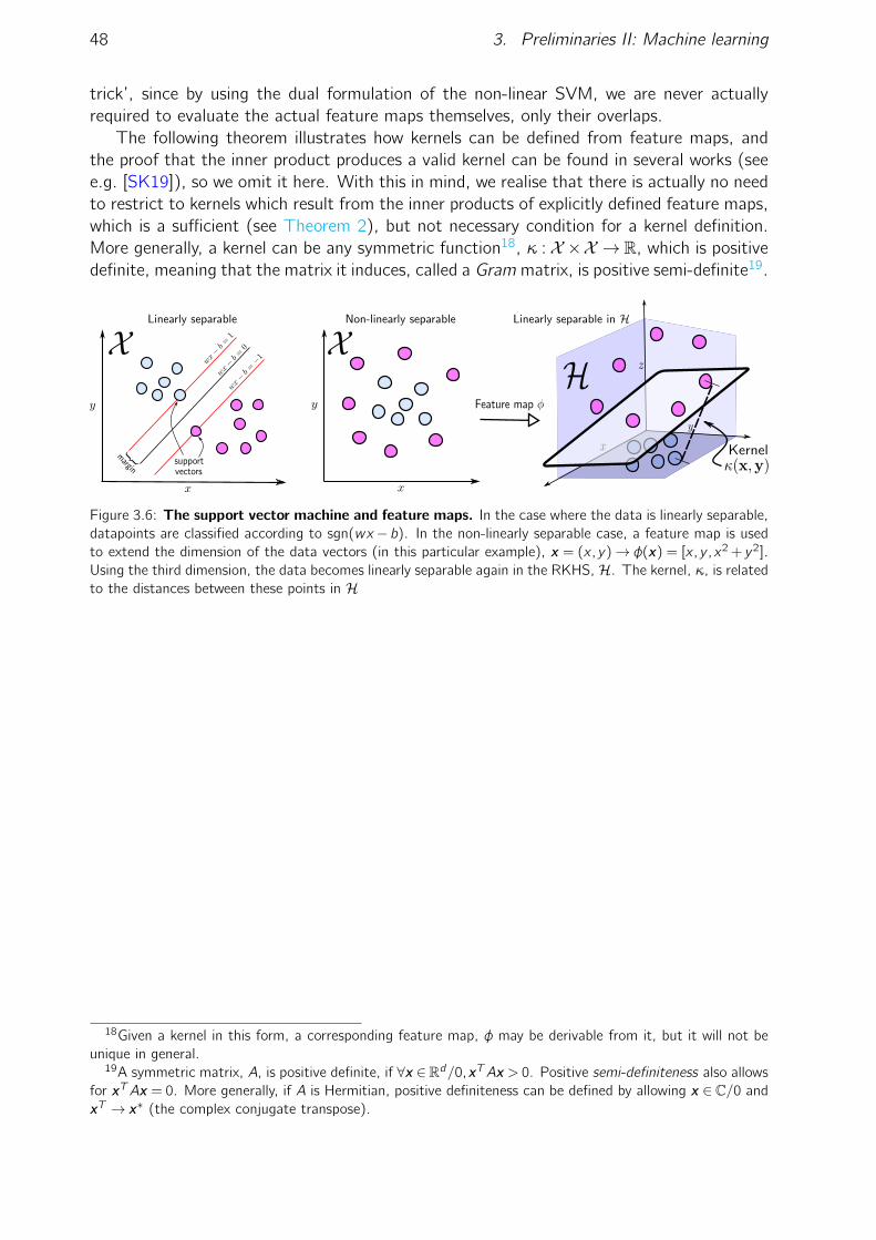
48 3. Preliminaries II: Machine learning
trick’, since by using the dual formulation of the non-linear SVM, we are never actuallyrequired to evaluate the actual feature maps themselves, only their overlaps.
The following theorem illustrates how kernels can be defined from feature maps, andthe proof that the inner product produces a valid kernel can be found in several works (seee.g. [SK19]), so we omit it here. With this in mind, we realise that there is actually no needto restrict to kernels which result from the inner products of explicitly defined feature maps,which is a sufficient (see Theorem 2), but not necessary condition for a kernel definition.More generally, a kernel can be any symmetric function18, κ :X ×X →R, which is positivedefinite, meaning that the matrix it induces, called a Gram matrix, is positive semi-definite19.
Figure 3.6: The support vector machine and feature maps. In the case where the data is linearly separable,datapoints are classified according to sgn(wx −b). In the non-linearly separable case, a feature map is usedto extend the dimension of the data vectors (in this particular example), x = (x,y)→ φ(x) = [x,y ,x2 + y2].Using the third dimension, the data becomes linearly separable again in the RKHS, H. The kernel, κ, is relatedto the distances between these points in H
18Given a kernel in this form, a corresponding feature map, φ may be derivable from it, but it will not beunique in general.
19A symmetric matrix, A, is positive definite, if ∀x ∈Rd/0,xTAx > 0. Positive semi-definiteness also allowsfor xTAx = 0. More generally, if A is Hermitian, positive definiteness can be defined by allowing x ∈ C/0 andxT → x∗ (the complex conjugate transpose).

3.6. Learning theory 49
For completeness, we also need to make sure that the inner products of feature maps doactually produce valid kernels (in the sense of being symmetric and positive definite. Thisfact is ensured by the following theorem, whose proof can be found in several works (seee.g. [SK19]), so we omit it here:
Theorem 2: (Feature map kernel)Let φ :X →H be a feature map. The inner product of two inputs, x ,y ∈ X , mappedto a feature space defines a kernel via:
κ(x ,y) := 〈φ(x),φ(y)〉H (3.19)
Note that the Hilbert feature space, H, is usually called a reproducing kernel Hilbertspace (RKHS). The ‘reproducing’ part arises because the inner product of the kernel at apoint in X , with a function, f ∈ H, in some sense evaluates or reproduces the function atthat point: 〈f ,κ(x , ·)〉 = f (x) for f ∈ H,x ∈ X . Now, let use return to the use of kernelsin a context more relevant for the contents of this thesis, i.e. as introduced in distributioncomparison measures such as the MMD in Sec. 2.1.7.1. In this case also, we use the kerneltrick to bypass difficult computations, and the feature maps allow us to map the samplepoints into a higher dimensional RHKS in which the distributions of interest may be moreeasily compared.
Let us conclude this section by mentioning some common examples of kernels. Theseinclude; the polynomial kernel (with degree d):
κP (x ,y) := (xT y +c)d , c > 0, (3.20)
The cosine kernel:κC(x ,y) := ∏
i=1ncos(x i −y i), (3.21)
The Laplace kernel:
κL(x ,y) := e−||x−y ||2
σ (3.22)
Or the mixture of Gaussians kernel:
κG(x ,y) :=1
c
c
∑i=1
e−||x−y ||22
2σi (3.23)
where σi are ‘bandwidth’ (hyper)parameters. The choice of the kernel function/featuremap (i.e. the choice of the RKHS) may allow different properties to be compared. Fora comprehensive review of techniques in kernel embeddings, see [MFSS17]. As mentionedabove, we discuss the generalisation of kernels to the quantum scenario in Sec. 4.2.
3.6 Learning theory
To conclude our preliminary material on (classical) machine learning, let us move from thecompletely practical in the training of neural networks, to the entirely theoretical realm atthe other end of the spectrum and discuss learning theory. Learning theory is the theoreticalframework which underpins machine learning, and tells us what things (functions, distribu-tions, quantum states, etc.) we can learn efficiently, and which things we cannot. It turns

50 3. Preliminaries II: Machine learning
out that there is a deep relationship between learning theory and cryptography, since manycryptographic primitives are based on objects which cannot be efficiently learned. A canon-ical example is the learning with errors problem, which is key to the field of post-quantumcryptography20. While this problem is now considered to be in the cryptography domain,its origins actually were formed in the context of learning.
While this topic may seem far removed from the contents of this Thesis, based on thetopics introduced previously, we emphasise it is not. In fact, we make a small contributionto quantum learning theory in Chapter 6 by discussing the learnability of distributions ina quantum setting, and also make a connection between quantum machine learning andquantum cryptography in Chapter 7.
For now, let us set the scene by introducing the most common and well studied learningscenario, that of function learnability21. The primary question in this subfield are of thefollowing form: given a function family, F , can we efficiently learn a representation of anyfunction, f ∈ F? While one may consider learning f exactly, it is perhaps more commonto instead consider learning approximately and with high probability. This learning model iscalled probably approximately correct (PAC) learning. Furthermore, we usually refer to Fas a concept class instead of a function family, and the requirement of a learning algorithmis to output a candidate function, h (a ‘hypothesis’), to a given ‘concept’, f ∈ F , which isnot too different from f on most possible inputs, x , from some space, X . For this section,we use the notation of [AdW17a] and the more interested reader may look further into thispaper and the references therein. Let us begin by defining what we mean by a learner:
Definition 18 (PAC function learning).A learning algorithm, A, is an (ε,δ)-PAC learning for a concept class, F if:For every f ∈ F , and every distribution, D, given access to a PEX(c,D) oracle, Aoutputs a hypothesis, h such that:
Pr (h(x) 6= f (x))6 ε (3.24)
with probability at least 1− δ.
PEX(f ,D) in the above is a ‘random example oracle’, which when queried, outputs alabelled example, (x , f (x)) where x is sampled from some distribution, D : 0,1n→0,1.This model is suitable for the supervised learning problem we discussed in Sec. 3.3.1, sincethe PEX oracle can be viewed as exactly providing one datapoint in a labelled dataset,see Definition 13.
Besides a random example oracle, one may consider alternative query models to thefunction family, including membership queries (where the learner provides x and the oraclereturns f (x)), or alternative learning models such as exact or agnostic learning [AdW17b],or learning under specific distributions (rather than every distribution as in Definition 18).
One of the key quantities which one may care about in learning theory is the samplecomplexity of learning the function. This is simply how many labelled examples does A
20Post-quantum cryptography is the study of primitives which are secure even in the presence of quantumcomputers (hence in a ‘post-quantum’ world). This was necessitated as a result of the ‘hackability’ of RSA-based cryptosystems with Shor’s algorithm. See e.g. [BL17] for a review of this field.
21Computational learning theory is a large field, and we do not attempt to even mention all possibleextensions one may consider. For a (quite outdated now) overview of some topics in the field, see [Ang92,KV94]

3.6. Learning theory 51
require, in order to output a sufficiently good hypothesis. In the classical domain (andindeed in the quantum domain also), this quantity, M, is given by the so-called VapnikChervonenkis (VC) dimension, which is a combinatorial quantity depending on the conceptclass, defined as:
Definition 19. (VC dimension [VC15].)Fix a concept class, F , over 0,1n. A set S = s1, . . . , st ⊆ 0,1n is said to be‘shattered ’ by a concept class, F if [f (s1) · · · f (st)] : f ∈F= 0,1t . In other words,for every labelling, `∈ 0,1t , there exists a f ∈F such that [f (s1) · · · f (st)] = `. TheVC dimension of F , VCdim(F), is the size of a largest S ⊆ 0,1n that is shatteredby C.
The result of [BEHW89, Han16] shows that M is exactly determined by VCdim(F):
Theorem 3: ([BEHW89, Han16, AdW17a])Let F be a concept class with VCdim(F). Then:
M = Ω
(VCdim(F)−1
ε+
log(1/δ)
ε
)(3.25)
examples are necessary and sufficient for an (ε,δ)-PAC learner for F .
With that, we conclude our discussion of function learning theory in the classical world -in the next section, Chapter 4, we will briefly introduce the quantum generalisations of theabove definitions, and in Chapter 6, we present the extension of these definitions into thedistribution (rather than function) learning setting.

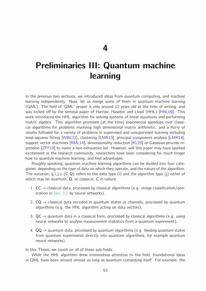
4
Preliminaries III: Quantum machinelearning
In the previous two sections, we introduced ideas from quantum computing, and machinelearning independently. Now, let us merge some of them in quantum machine learning(QML). The field of ‘QML’ proper is only around 12 years old at the time of writing, andwas kicked off by the seminal paper of Harrow, Hasidim and Lloyd (HHL) [HHL09]. Thiswork introduced the HHL algorithm for solving systems of linear equations and performingmatrix algebra. This algorithm promised (at the time) exponential speedups over classi-cal algorithms for problems involving high dimensional matrix arithmetic, and a flurry ofresults followed for a variety of problems in supervised and unsupervised learning includingleast-squares fitting [WBL12], clustering [LMR13], principal component analysis [LMR14],support vector machines [RML14], dimensionality reduction [KL20] or Gaussian process re-gression [ZFF19] to name a non-exhaustive list. However, will this paper may have sparkedexcitement in the research community, researchers have been considering for much longerhow to quantize machine learning, and find advantages.
Roughly speaking, quantum machine learning algorithms can be divided into four cate-gories, depending on the type of data on which they operate, and the nature of the algorithm.The notation, ij, i, j ∈ C,Q refers to the data type (i) and the algorithm type (j) either ofwhich may be quantum, Q, or classical, C in nature:
1. CC→ classical data, processed by classical algorithms (e.g. image classification/gen-eration in Sec. 3.1 by neural networks).
2. CQ→ classical data encoded in quantum states or channels, processed by quantumalgorithms (e.g. the HHL algorithm acting on data vectors),
3. QC→ quantum data in a classical form, processed by classical algorithms (e.g. usingneural networks to analyse measurement statistics from a quantum experiment),
4. QQ→ quantum data, processed by quantum algorithms (e.g. feeding quantum statesfrom quantum experiments directly into quantum algorithms, for example quantumneural networks).
In this Thesis, we touch on all of these sub-fields.While the HHL algorithm drew tremendous attention to the field, foundational ideas
in QML have been around almost as long as quantum computing itself. For example, the
53

54 4. Preliminaries III: Quantum machine learning
typography of QML algorithms discussed above was introduced early on in 2006 by [ABG06].Bshouty and Jackson initiated quantum learning theory (the quantum analogue of thatpresented in Sec. 3.6) in 1995 by generalising probably approximately correct (PAC) learningto the quantum setting [BJ95] (we will return to this topic later in this Thesis). Finally,proposals for ‘quantum’ neural networks appeared as early as 1996 [BNSS96], the same yearas the canonical Grover search algorithm [Gro96]. Indeed, a well-accepted definition for aquantum version of a neural network is still elusive to date [SSP14], with the ‘non-linearity’(in Eq. (3.2) for example) being difficult to emulate quantumly. As mentioned in Sec. 3.1,the most widely accepted model (at the current time) for a quantum neural network is basedon the parametrised quantum circuit (PQC) which is the key component of this Thesis.
Since the development of HHL, QML development has experienced what could be calledtwo ‘waves’ of progress. The first wave focused around ‘coherent’ algorithm development,primarily using methodologies pioneered by HHL (such as the examples listed at the startof this chapter). The second wave was born with the introduction of the PQC and thevariational algorithm. The algorithms in the former case are widely believed not to beimplementable on quantum hardware for many years to come, as they require large num-bers of error corrected qubits (hence the nomenclature ‘coherent’), and deep circuits toguarantee the speedups they promise. In contrast, variational quantum algorithms1 (alsodubbed ‘modern’ quantum algorithms [Bia20]) in the second wave are heuristic in nature,and as such they do not usually have provable guarantees of runtime complexity. However,they are readily implementable on the quantum computers available now, many of whichare accessible remotely through the ‘quantum cloud’ [LaR19]. Early work in QML algo-rithms almost exclusively focused around quantum speedups in runtime. However, speedis not the only way to measure a ‘quantum advantage’ over classical methods for ma-chine learning tasks. Indeed, one may consider other avenues along which to search fora quantum advantage (but not limited to: expressibility, accuracy, interpretability, privacyand generalisability). The simultaneous rapid development of quantum computing hard-ware since ∼ 2010 means that building and experimenting with real quantum models isaccessible to anyone with an internet connection, and as such current research has partiallyshifted away from that of purely theoretical algorithm proofs to more experimental andexploratory in nature. For completeness, we mention some examples of quantum machinelearning which do not quite fit into these categories, including speedups (however not expo-nential) in training Boltzmann machines [WKGS15], or building quantum models based onquantum annealing hardware, including the quantum Boltzmann machine [KW17, AAR+18,BRGPO18, WVHR19, WW19]. One may also consider advances in quantum reinforcementlearning [DCLT08, DTB17, DLWT18, LS20a, JTPN+21, JGM+21, SJD21]
For coherent algorithms in the first wave, a crucial ingredient is required. This is theability to access data ‘in superposition’. Specifically, these algorithms usually require one tobe able to prepare states of the form:
|x〉=n
∑i=1
xi |i〉 (4.1)
1Variational algorithms are actually used for more general purposes than simply machine learning (meaningdata-driven) applications. However, the core of both variational algorithms and heuristic quantum machinelearning algorithms reduces to the optimisation of some parametrised object (typically a parametrised quantumcircuit). Hence, we use both terms interchangeably in this Thesis to refer to the same concept.

4.1. Variational quantum algorithms 55
Where x = [x1, . . . ,xn]T ∈ Rn, is a data vector2. This is the so-called amplitude ([SP18,ZFR+21]) encoding and the procedure to prepare such a state is called a ‘data-loading’routine. We return to data encoding in Sec. 4.1.4 and Chapter 5. Once amplitude encodedstates are prepared, they are further processed by the quantum algorithm. However, whenconsidering the true runtime of such algorithms, one must also factor in the cost of preparingsuch states. As stated by [Aar15], if a routine to prepare Eq. (4.1) required nc steps (forsome constant c), then speedups are lost.
In principle, such data-loading issues can be sidestepped by the existence of a quantumrandom access memory3 (QRAM) [GLM08], acting as follows on a superposition of ‘address’registers, |i〉:
1√N
n
∑i=1
|i〉 −−−−→QRAM
1√N
n
∑i=1
|i〉|xi〉 (4.2)
However, constructing such a quantum memory which can be accessed in superpositionmay be as hard as building a fully fault tolerant quantum computer. As we hinted at above,there are also many other practical issues with these ‘coherent’ QML algorithms (such asHHL) that need to be carefully addressed in order determine whether speedups are actuallyfeasible [Aar15]. For an overview of technical details used in such linear system algorithms,see [DHM+18] which also discusses constructions for QRAM objects.
Finally, we would be remiss if this Thesis included a section introducing quantum ma-chine learning without mentioning the ‘dequantisations’. In 2018, [Tan18a] proposed afully classical algorithm to kill the exponential speedup of one of these coherent algo-rithms - the ‘quantum recommendation system’ algorithm of [KP16]. Previously, thisquantum algorithm was one of the most promising candidates for an end-to-end expo-nential speedup over its classical counterparts. The classical algorithm of Tang howeverdemonstrated this was not the case, and the advantage of [KP16] was reduced to onlypolynomial4 We highlight this to demonstrate how subtle the nature of quantum advantageis in QML. For those interested in further reading of ‘dequantised’ quantum algorithms,see [Tan18b, GLT18, CLW18, CGL+20, SM21] and also [ADBL20] for a study of thesealgorithms in practice.
Before moving to the next section, we conclude by highlighting some reviews of quantummachine learning including [Wit14, SSP15, BWP+17, DB18, BLSF19] which discuss manyof the topics we neglected here.
4.1 Variational quantum algorithms
This Thesis however is focused solely on algorithms in the second wave, the variationalquantum algorithms (VQAs). As mentioned above, VQAs (also called ‘near-term’ quantummachine learning algorithms) are a powerful model for quantum algorithm design on NISQdevices. Fig. 4.1 gives an overview of some of the key ingredients involved. VQAs are char-acterised by a quantum component, and a classical component, which work synergisticallyto solve the problem of interest. In order to maximise the use of quantum coherence time
2Assuming the vectors are normalised such that ||x ||2 = 1.3Similarly to a classical RAM, which returns the contents of a memory register when accessed.4However, we remark that this is not so much of a blow as it seems, the constant factors in the original
algorithm of [Tan18a] indicated that the quantum algorithm could still be significantly faster. The most recentanalysis by [SM21] indicated that this speedup is only quadratic in reality for a special case of the problem.

56 4. Preliminaries III: Quantum machine learning
(which is limited by the lack of error correction in NISQ devices), the majority of the compu-tation is carried out by the classical device, which performs the task of optimising the param-eters of a quantum object (typically a parametrised quantum state) to solve the problem.
Figure 4.1: Cartoon illustration of a variationalquantum algorithm.
The quantum component may have someinput, |ψ〉in, and produces some outputstate, ρθout, which is parametrised by θ. Inorder to apply a general quantum transfor-mation, the quantum component may inter-act with an environment (described by an-cillary registers), and from the output stateseveral observables may be measured, Oi .These classical results are then passed intoa classical computer which computes somecost function of these observables and findsparameter updates θ→ θ′ (via gradient de-scent or otherwise) to drive the computa-tion. These approaches are clearly heuris-tic in nature, however some effort has beenmade to study them from a theoretical pointof view [MRBAG16, Bia20] and the compu-
tational model they exhibit is actually also universal for quantum computation [Bia19] despiteonly using short depth quantum circuits.
At this point, if we replace the quantum device by a neural network5, the connection tomachine learning becomes clear. To introduce the relevant concepts in this section, we useand refer to the following reviews, [CAB+21, BCLK+21, ECBY21]. Key concepts involvedin variational quantum algorithms, are:
• The cost function defining the problem.
• The ansatz used by the quantum computer.
• The optimisation of the cost function.
• The input to the VQA (some form of data encoding for classical data).
• The desired output - measurement readout, or quantum states.
In the subsequent sections, we introduce each of these to the degree of detail for whichthey are relevant in this Thesis.
4.1.1 The cost function
Just as in classical machine learning, the problem to be solved can be reduced to optimisinga cost function, which is some function of the parametrised state:
minθ
C(θ) (4.3)
5In fact, a more general scenario is where some function is applied to the output measurements from thequantum circuit before passing it to a classical optimiser. This function may be simple, or may be the outputof another classical neural network. We do not consider this possibility in this Thesis, so we neglect it forsimplicity.

4.1. Variational quantum algorithms 57
The choice of cost function is crucial for the success of VQAs, and not surprisingly, this factoriginates from their machine learning origins. Concretely, four desirable qualities for VQAcost functions are ([CAB+21]):
Faithfulness. Efficientlycomputable.
Operationalmeaning.
Trainable.
1. Faithfulness: The minimum point θ∗ := argminC(θ), is the solution to the problemof interest in the parameter space6.
2. Efficiently computable: It should be possible to estimate C to a reasonable precisionwith polynomial resources (number of qubits, gates in the circuit, etc.).
3. Operational meaning: Smaller cost values correspond to higher quality solutions.
4. Trainable: The cost should be optimisable in an efficient way (efficiently computablegradients, navigatable parameter space, etc.).
For many variational algorithms, the problem can be encoded as a ground state opti-misation problem, meaning that the problem parameters are encoded into a Hamiltonian,H, and the solution is encoded in the ground state of this Hamiltonian (the state with theminimum energy). In this case the optimisation becomes:
minθ〈ψ(θ)|H|ψ(θ)〉 := Eθ∗ (4.4)
The goal is to find the eigenstate, |ψ(θ∗)〉, with the lowest energy, Eθ∗. VQAs in this formare known as variational quantum eigensolvers (VQE), which was one of the original VQAproposals by [PMS+14] that pioneered the field. VQE caused a great deal of excitementdue to its applicability to quantum chemistry [MEAG+20] problems and quantum simula-tion [CMMS20]. In these cases, the Hamiltonian, H, is the one defined by the physicalsystem to be simulated, and is the source of the observables, Oi , to be measured. Forexample, in finding the ground state of the Ising model Hamiltonian acting on N spins:
Hising :=N
∑i<j
Ji jZi ⊗Zj +N
∑k=1
bkZk , (4.5)
the observables to be measured are the correlations 〈Zi ⊗Zj〉ψ and the local expectations〈Zk〉ψ7. Each of these observables is measured8, and the results are collected (and weightedby the coefficients Ji j ,bi) to compute the energy of the system when in the state, |ψ〉.
Cost functions are highly problem dependent, those in the form of Eq. (4.4) are amongthe simplest, but in the case of machine learning problems particularly, the choice of costfunction is complex and crucial to the success of the algorithm. As such, one can generalisecost functions into the following form [CAB+21]:
C(θ) = ∑k
fk(Tr[Okρθout]) (4.6)
6The parameter space is the multidimensional space described by the parameters, θ.7〈O〉ψ denotes the expectation value of the operator, O, with respect to the state, |ψ〉: 〈ψ|O|ψ〉.8Since all terms in this Hamiltonian commute, these statistics can all be collected using a single measure-
ment setting, by measuring every spin (qubit) in the computational basis.

58 4. Preliminaries III: Quantum machine learning
where fkk are a set of functions applied to the output. In this Thesis, cost function choicewill play an important role.
Local versus Global Cost Functions
Before moving on, let us highlight one important generic feature of VQA cost functions;their locality. Namely, whether the observables involved in computing C are either local orglobal. Roughly speaking, local observables are those consisting of a function of terms whicheach can be computed by only measuring a handful of qubits, whereas global cost functionsrequire information about the entire quantum state. For example, the cost function definedby VQE on the Ising model Hamiltonian, Eq. (4.5) is 2-local since the terms in it requiremeasuring no more than 2 qubits at a time (the terms Zi ⊗Zj only operate on two qubits,i , j , and Zk only acts on qubit k). In the case of VQE problems, the locality of the costfunction directly relates to the locality of the Hamiltonian in question which is a well-studiedtopic [KKR06], but it is a more general concept.
Specifically a k-local cost function observable can be written as ([CSV+21]):
O = c01+N
∑i=1
ci Oki (4.7)
where each Oki are k-local operators, acting at most on k ⊂ [n] qubits. In contrast, a globalcost function has the form:
O = c01+N
∑i=1
ci O1i ⊗ Oi2⊗·· ·⊗ Oin (4.8)
In both cases, N is the number of terms given by the problem of interest and c0,ci arecoefficients which can assumed to be real WLOG (e.g. corresponding to Ji j ,bk in Eq.(4.5)).
Cost function locality is also important regarding operational meaning. Typically, fromthis point of view, global cost functions are usually more favourable since they can be directlyinterpreted. In variational compilation [KLP+19], the cost function compares the similarityof two global unitaries, and is zero when the unitaries are identical. In contrast, local costfunctions are perhaps less interpretable, but can usually be used as a bound to optimisea global cost. Furthermore, as we shall discuss in Sec. 4.1.3, local unitaries are usuallyeasier to optimise than their global counterparts ([CSV+21]). We return to this discussionin Chapter 7.
4.1.2 Ansätze
The second important ingredient in VQAs is the ansätze, for the parametrised state, i.e.the operation that performs the mapping |ψ〉in→ ρθout in Fig. 4.1. In VQAs, the ansatz9 isusually a unitary transformation:
|ψ(θ)〉= U(θ)|ψ〉in, ρθout := |ψ(θ)〉〈ψ(θ) | (4.9)
9Historically, an ansatz in physics is an ‘educated guess’ for a problem solution. This has translated intoquantum computing in preparing the ‘trial’ state for a VQA.
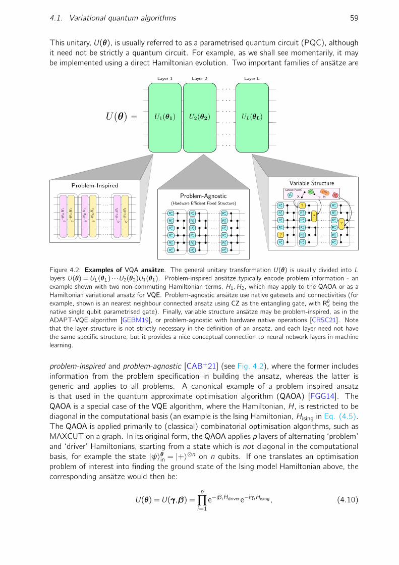
4.1. Variational quantum algorithms 59
This unitary, U(θ), is usually referred to as a parametrised quantum circuit (PQC), althoughit need not be strictly a quantum circuit. For example, as we shall see momentarily, it maybe implemented using a direct Hamiltonian evolution. Two important families of ansätze are
Figure 4.2: Examples of VQA ansätze. The general unitary transformation U(θ) is usually divided into Llayers U(θ) = UL(θL) · · ·U2(θ2)U1(θ1). Problem-inspired ansätze typically encode problem information - anexample shown with two non-commuting Hamiltonian terms, H1,H2, which may apply to the QAOA or as aHamiltonian variational ansatz for VQE. Problem-agnostic ansätze use native gatesets and connectivities (forexample, shown is an nearest neighbour connected ansatz using CZ as the entangling gate, with Rθx being thenative single qubit parametrised gate). Finally, variable structure ansätze may be problem-inspired, as in theADAPT-VQE algorithm [GEBM19], or problem-agnostic with hardware native operations [CRSC21]. Notethat the layer structure is not strictly necessary in the definition of an ansatz, and each layer need not havethe same specific structure, but it provides a nice conceptual connection to neural network layers in machinelearning.
problem-inspired and problem-agnostic [CAB+21] (see Fig. 4.2), where the former includesinformation from the problem specification in building the ansatz, whereas the latter isgeneric and applies to all problems. A canonical example of a problem inspired ansatzis that used in the quantum approximate optimisation algorithm (QAOA) [FGG14]. TheQAOA is a special case of the VQE algorithm, where the Hamiltonian, H, is restricted to bediagonal in the computational basis (an example is the Ising Hamiltonian, Hising in Eq. (4.5).The QAOA is applied primarily to (classical) combinatorial optimisation algorithms, such asMAXCUT on a graph. In its original form, the QAOA applies p layers of alternating ‘problem’and ‘driver’ Hamiltonians, starting from a state which is not diagonal in the computationalbasis, for example the state |ψ〉θin = |+〉⊗n on n qubits. If one translates an optimisationproblem of interest into finding the ground state of the Ising model Hamiltonian above, thecorresponding ansätze would then be:
U(θ) = U(γ,β) =p
∏i=1
e−iβiHdrivere−iγiHising, (4.10)

60 4. Preliminaries III: Quantum machine learning
where Hdriver =⊗nj=1Xj is the driver Hamiltonian for which the initial state, |+〉⊗n ,is an
eigenstate. Each ‘layer’ in the ansatz has 2 free parameters, so the optimisation requiresfinding 2p optimal parameters.
This ansatz type has been generalised to the alternating operator ansatz10 [HWO+19]which can encode different symmetries of the problem and may improve performance. Asecond type of ansatz is a further generalisation of the QAOA ansatz, called the Hamiltonianvariational ansatz, and is used when the problem Hamiltonian is not diagonal, i.e. in VQEproblems. In this case, the Hamiltonian can be split into multiple non-commuting terms,Hk [CAB+21],
U(θ) = ∏l
(∏k
e−iθl ,kHk
), (4.11)
Again, the ansatz is applied for a number of layers. Both of these ansätze derive inspirationfrom the quantum adiabatic algorithm [FGGS00], and Trotterization methods for quantumsimulation, which are used for simulating the evolution of a system. For the latter case inVQE, the initial state is usually also problem inspired, for example the Hartree-Fock groundstate, which is exactly solvable for a given system.
The second class of ansätze are the problem-agnostic, which usually aim to reducethe circuit depth and number of gates required to implement them (in contrast to thealternating operator/Hamiltonian variational ansätze, which may require significant depthto implement). Furthermore, the operations in agnostic ansätze are usually hardware-native.For example, to implement a hardware-native ansatz on Rigetti [SCZ17] one may use theCZ or XY gates for entanglement creation, whereas for IBM quantum computers, one wouldchoose a directed CNOT. Using native gates dispenses with the need to perform extensivecompilation and so keeps the circuits shallow. Furthermore, only allowing the connectivitybetween qubits which is directly accessible on the quantum device also is essential for highperforming results on NISQ hardware11.
The most common problem-agnostic ansätze are called hardware-efficient. Two specificforms of hardware efficient ansätze are used in this Thesis. The first are fixed-structure,which contain a number of layers, where each layer has a fixed structure of entangling andsingle qubit rotations12
The second class of hardware-efficient ansätze are variable-structure ansätze. In thesecircuits, not only are the continuous gate rotations optimised over, but also the gatesin the circuit themselves. A fixed-structure ansatz may require several layers to solve agiven problem, in contrast variable-structure ansätze are capable of finding circuits with theabsolute minimum number of quantum gates. Formally, this corresponds to a more generaloptimisation problem than Eq. (4.3):
(θ∗,g∗) = argminθ,g∈G
C(θ,g) (4.12)
10Which also offers the acronym QAOA, confusingly.11Compilation may significantly increase the circuit depth in a NISQ circuit implementation. If an algorithm
requires a CNOT, but only CZ is available natively, two H gates will need to be added to change the basis.Secondly, performing qubit routing to apply a transformation between two qubits which are not directlyconnected is expensive - a single SWAP gate requires 3 CNOT gates to implement.
12For ease of implementation, when dealing with hardware efficient ansätze in this Thesis, we assume thattwo qubit unitaries are un-parametrised (meaning implemented with a fixed parameter), and the trainableparameters, θ, are only contained in single qubit rotations. This is not a necessary assumption in general.

4.1. Variational quantum algorithms 61
Here, G is a gateset pool, g corresponds to a certain sequence of gates in the pool. Clearly,the problem now becomes a discrete optimisation problem as well as a continuous one (westill need to optimise over the gate parameters, θ).
The variable-structure approach was given proposed in [CSSC18], and variations onthis idea have been given in many forms [OGB21, RHP+20, LFC+20, PT21]. Most re-cently, these ideas have been given the broad classification of quantum architecture search(QAS) [ZHZY20] to draw parallels with neural architecture search [YWC+19, LSY19],(NAS)13 in classical ML. We also mention that the variable-structure approach is not onlyrestricted to be used with a hardware-efficient ansatz. Indeed, a variation has been used onthe Hamiltonian variational ansatz for VQE ([GEBM19, CSU+20]) and for QAOA [ZTB+20].One interpretation of QAS is its use in discovering novel primitives (we apply it to the prim-itive of quantum cloning in Chapter 7) for quantum algorithms, protocols or experiments;QML for primitive discovery if you will. Interestingly, a parallel and related line of work hasalso been progressing using purely classical machine learning in discovering novel quantumprotocols and experiments [KMF+16, MNK+18, WMDB20].
Finally, it is also crucial to mention that for machine learning applications, good ansätzedesign is still an open area of research. A primary reason for this is the data-driven natureof ML which makes definition of a ‘problem-inspired’ ansatz difficult. The choice is perhapsmore natural when examining quantum machine learning for quantum data, where onecan use a physically inspired ansatz which may encode certain problem symmetries. Forexample, a proposal for a quantum convolutional neural network [CCL19] (QCNN) usesa translationally invariant structure which may be suitable for physical systems with thisproperty, or defining Hamiltonian-based models [VMN+19] as ansätze which can learn torepresent mixed quantum states.
4.1.3 Cost function optimisation
Once a suitable cost function has been chosen, the question then becomes how one canoptimise it to solve the problem. In the above VQE example, this corresponds to finding theoptimal parameter setting, θ∗, as a proxy for optimising over the set of possible quantumstates to find the ground state of the Hamiltonian in question.
As with neural network training, optimisation routines for cost functions can be broadlygrouped into two categories: gradient-free and gradient-based. Criteria number four ofdefining useful cost functions indicates they must be efficiently trainable (similarly again tothe neural network training in Sec. 3.2. This means (in the case of gradient-based optimi-sation) that they must have efficiently14 computable gradients.
4.1.3.1 Gradients
Fortunately, for many VQAs, this is the case. Specifically, if the gates in the VQA ansatz,U(θ), are of a particular form, the gradients of the cost function can be computed an-
13NAS is the analogous task for finding optimal structures in neural network architectures, for exampletuning the width and depth of the network.
14Efficient here usually refers to with respect to the number of qubits, N, but also all other relevantparameters of the problem.

62 4. Preliminaries III: Quantum machine learning
alytically, using what is known as the parameter-shift rule [MNKF18, SBG+19, BIS+20,SWM+20, HN21] which we alluded to previously:
The parameter-shift rule:Given a cost function, C, which is evaluated using an ansatz (with L parameters)containing quantum operations of the form U(θi) = e−i(θi/2)Σ, where Σ2 = 1, thegradient of C with respect to a particular parameter θi is given by:
∂C(θ)
∂θi:= ∂θi C(θ) =
1
2
[C(θ+
i )−C(θ−i )], (4.13)
where θ±i = (θ1,θ2, . . . ,θi ± π2 , . . . ,θL)
Note also that the expression in Eq. (4.13) is exact, and the shift constant π/2 is large,in contrast to the infinitesimally small shifts and approximate nature of methods such asfinite-difference15. However, since C is estimated by running a circuit on a quantum device,we cannot extract the exact value C without an infinite number of measurement shots. Assuch, we will only have access to estimates, C and ∂C of the cost and its gradients.
Interpreting Eq. (4.13), we see that we can evaluate the gradient of a cost with respectto any particular parameter by simply computing the cost twice in a ‘parameter-shifted’fashion. As such, if we assume a complexity of T for evaluating C, then we will occur anoverhead of 2L×T to evaluate the gradients for all L parameters in the ansatz, and so if thecost is efficient to compute, so are its gradients. However, comparing this black-box typecomputation (since the parameters must be evaluated independently) to the efficiency ofthe backpropagation algorithm we discussed in Sec. 3.4, where we can ‘reuse’ computationsfrom one layer to another, we see this linear scaling may be an expensive16 price to pay.Nonetheless, many quantum software libraries including TensorFlow Quantum [BVM+20] byGoogle, or Pennylane [BIS+20] by Xanadu offer these gradient computations incorporatedto the standard deep learning libraries such as TensorFlow or PyTorch. One can circumventthis linear scaling by using a quantum simulator to train quantum models, as direct accessto the wavefunction allows the implementation of autodiff methods. However, this isclearly not possible if training a (near term) model on quantum hardware, and at the timeof writing, this linear scaling is the best we have.
A final point to note is the assumption that Σ2 = 1 in the above theorem. This isnot in fact necessary, and the theorem has been extended in many aspects, includingstochastic versions for more general operations [Cro19] higher order [MBK21] and natu-ral gradients [SIKC20, KB20a], imaginary time evolution [MJE+19], and analytic meth-ods ([OGB21, KB20b, CMMS20]) have been proposed. This is an active area of research,and this Thesis will only require the simplest forms of gradient descent using the parameter-shift rule in the form given above, so we neglect further discussion of other methods.
15See [MBK21] for a comparison between parameter-shift and finite-difference methods.16If we treat the cost function in the quantum and classical cases as an oracle, we are only counting
the number of evaluations which must be done for each parameter. A discussion of the quantum/classicalcomputability of the cost is a separate question.

4.1. Variational quantum algorithms 63
4.1.3.2 Barren plateaus
The problems mentioned relating to VQA optimisation are also common to machine learning,but the nature of VQAs also introduces unique problems. These problems manifest in thecost function landscape and two phenomena are called barren plateaus (BPs) and narrowgorges. Barren plateaus are exponentially flat regions in the parameter space, in whichgradient-based17 optimisation will fail, since the gradient of the cost function is close tozero in all directions.
Definition 20 (Barren plateau (from [AHCC21])).Consider a VQA cost function defined as in Eq. (4.6) with fk(x);= akx,ak ∈ R. Thecost exhibits a barren plateau if ∀θ ∈ θ, the variance of its partial derivative vanishesexponentially with n, the number of qubits:
Varθ[∂θi C(θ)]6 F (n), with F (n) ∈ O(b−n) (4.14)
for some b > 1. The expectation values are taken with respect to the parameters, θ:Varθ[∂θi C(θ)] = 〈[∂θi C(θ)]2〉θa.
aFor proofs it is usually assumed that the expectation is computed over unitaries that contain theparameters, and furthermore that these unitaries form exact ([MBS+18]) or approximate ([HSCC21])quantum t-designs [DCEL09] in order to make the integration tractable.
This phenomenon was first observed by [MBS+18] which found that such plateaus oc-curred in sufficiently deep random (and hardware-efficient) PQCs. This was extended in[CSV+21] and found to occur with much shallower circuit depths and be highly dependenton the locality of the cost function. Entanglement, a key resource in quantum computation,was also proven to be detrimental to training PQCs as too highly entangled systems wereshown to exhibit also a BP [MKW21].
Of interest to note, is the ansatz dependent nature of barren plateaus - they arerigorously proven to exist primarily for hardware efficient ansätze, but have proven tobe absent in quantum convolutional neural networks [PCW+20] or tree tensor networkbased ansätze [ZG21, ZHLT20]. Furthermore, using problem-inspired ansätze such asthe Hamiltonian variational ansatz has been shown numerically to be useful for mitigatingBPs [WZdS+20]. Finally, the barren plateaus referenced above originate from the random-ness in such circuit designs, and as such would exist even if VQAs were implemented onfault-tolerant quantum devices. For near term NISQ hardware unfortunately, an alternateBP rears its head. Dubbed ‘noise-induced’ barren plateaus [WFC+21], these arise simplydue to hardware noise on quantum devices, and may prove to be an alternative roadblockin the usefulness of VQAs.
Hope, however, is not lost. While the discovery of BPs have proliferated, so too havestrategies to mitigate them, ranging from clever initialisation strategies [GWOB19] andcorrelating parameters [VC21] to using entanglement as a resource [PNGY20].
Complementary to BPs, we also have the ‘narrow gorge’ phenomenon. This states thatthe problem solution occurs in a deep gorge with a small width which shrinks exponentiallyquickly as the problem size increases. The narrow gorge has been less well studied to date,
17This is not in fact limited to gradient methods, it has also been shown that gradient-free methods whichrely on cost function differences will also fail[ACC+20]

64 4. Preliminaries III: Quantum machine learning
so we will not focus on it in this Thesis, but its appearance in a cost landscape was provento be synonymous with a barren plateau - one never occurs without the other [AHCC21].This observation led to the definition of quantum landscape theory [AHCC21], which aimsto thoroughly investigate parameter landscapes.
Given the above discussions, barren plateaus and landscape study is an active area ofstudy and highly interesting. This is particularly true given their impact on discoveringpractical applications of quantum computers, which is the main goal of this Thesis. Wereturn to a discussion of BPs later for our specific use case.
4.1.4 VQA inputs and outputs
The nature of the inputs and outputs of a VQA are highly problem dependent. We havetouched on some of these in the above sections, but now let us highlight some key examplesin more detail. When using VQAs as machine learning applications on classical data, the datamust be encoded in quantum states to be processed by the ansatz. Similarly, in these casesthe outputs must also be classical, which corresponds to performing some measurementson the quantum state. However, for QML/VQA applications on quantum data, quantumstates are directly provided as training data ρiMi=1 to the algorithm. Depending on thenature of the problem, the output for quantum data may be still classical, but in some casesthe VQA may output quantum states themselves as the solution18. We shall encounter anexample later in this Thesis which exactly falls in this latter category.
In order to motivate key concepts in this area, we proceed by discussing three examples,which will play central roles in the concepts used later in this Thesis. Let us begin with oneof the simplest possible:
• Data encoding for quantum classifiers.
A quantum classifier is one of the simplest applications one could consider for a VQA/QNN.To be clear, here we refer to quantum classifiers for classical data. As such, the problemstatement is exactly the same as in Sec. 3.3.1. Quantum classifiers for quantum data arean extremely interesting area of study (see [CCL19] for example) but outside the scope ofthis Thesis.
Given a classical dataset of N dimensional (real) vectors, D = xmMm=1, we must havesome method to encode or embed the datapoints, xm ∈RN into quantum states for furtherprocessing in the quantum classifier. For the remainder of this Thesis, we primarily focus ondata embeddings which encode only a data point per quantum state19. Such an encodingprocess is achieved by a state preparation operation, E, which acts as follows:
Eφ : x → ρφx (4.15)
In this Thesis, we assume an implementation of Eφ as a unitary, Sφ, acting on a fixed initial(pure) state, so:
Sφ(x)|0〉⊗n = |φ(x)〉 (4.16)
18Of course, even in these cases some classical information is usually extracted for the purposes of trainingthe PQC. There are also proposals for ‘quantum training’, which is done more coherently than is typical inVQAs [VPB18, KP20, LHF21]
19As opposed to data encodings which consider also a superposition over datapoints in the dataset, whichmay be required for some QML algorithms. An example is the amplitude encoding given in Eq. (4.1).

4.1. Variational quantum algorithms 65
The function φ is a ‘feature map’ which maps from the original data space, X , into a ‘featurespace’ (similar in nature to the feature map discussed for kernel methods in Sec. 2.1.7.1).The resulting state, |φ(x)〉 is therefore sometimes referred to as a quantum feature vector.For Sφ(x) to be useful as a data encoding, it should have several desirable properties. First,Sφ(x) should have a number of gates which is at most polynomial in the number of qubits aswell as the size of the dataset, dimension of the data to be encoded, and all other relevantinput parameters. For machine learning applications, we want the family of state preparationunitaries to have enough free parameters such that there is a unique quantum state ρx foreach feature vector x — i.e., such that the encoding function Eφ is bijective. Additionally,for NISQ applications, sub-polynomial depth is even more desirable, and we want Sφ(x) tobe hardware-efficient.
We have already encountered such a state preparation routine earlier in this Thesis in theform of the amplitude encoding (Eq. (4.1)). Data encoding methods are of key interest tothe success of QML algorithms in general, see [SP18] for an overview of encoding strategiesand techniques. For completeness, we list some example encoding methods (taken from[SP18, SK19]).
Definition 21 (Basis encoding).Given a feature vector x = [x1, ...,xN ]T ∈ 0,1N , the basis encoding maps x 7→EBasis
φ
as:
EBasisφ : x ∈ 0,1N → |φ(x)〉= |x〉
=⇒ SBasisφ (x)|0〉⊗n = Xx0⊗·· ·⊗XxN |0〉⊗n(4.17)
Definition 22 (Amplitude encoding).Given a feature vector x = [x1, ...,xN ]T ∈CN , the basis encoding maps x 7→ EAmp
φ as:
EAmpφ : x ∈ Cn→ |φ(x)〉=
1
||x ||2
N
∑i=1
xi |i〉 (4.18)
Here, we use n =O(log(N)) qubits to encode N-dimensional datapoints.
Definition 23 (Product (qubit) encoding).Given a feature vector x = [x1, ...,xN ]T ∈RN , the basis encoding maps x 7→EProd
φ=(fi ,gi )ni=1
given by
EProdφ=(fi ,gi )
ni=1
: x ∈ RN →N⊗i=1
[fi(xi)|0〉+gi(xi)|1〉] , |fi |2 + |gi |2 = 1, ∀i (4.19)
The canonical example for a product encoding is choosing fi = cos(xi),gi = sin(xi), ∀i .In this case we have Sφ(x) :=
⊗ni=1Ry (2xi), and the resulting state is:
|φ(x)〉=N⊗i=1
[cos(xi)|0〉+ sin(xi)|1〉] (4.20)
Finally, let us end this discussion with a reflection on the dimension, N, of the datapoints.In order to actually use the NISQ computers available today for classification dataset, we

66 4. Preliminaries III: Quantum machine learning
are limited to relatively small datasets. For example, if one tried to directly perform aclassification task on the MNIST dataset (the example in Sec. 3.3.1), each image consistsof 28×28 = 784 pixels, which means N = 784. However, no (universal) quantum computercurrently exists with 784 qubits, so encoding using the product or basis encodings is notpossible. In contrast, qubit efficient encodings such as the amplitude encoding would onlyrequire 10 > log(784) qubits, but may require a linear (relative to the length of vector tobe encoded) depth for the state preparation circuit, making it impractical to run on NISQdevices with short coherence times. An alternative name for state preparation circuits are‘data loaders’, and a family of such data loaders have been proposed with q qubits, anddepth D with overall complexity qD =O(N logN) [JDM+21], so it is likely either one mustsacrifice circuit depth or qubit number to load data. Alternative strategies for fitting largerdatasets on NISQ computers are, for example, using dimensionality reduction or featureextraction techniques such as principal component analysis (PCA) [GBC+18] to extract themost relevant features.
In summary, loading classical data into quantum states in NISQ devices is challengingin practice, but it is an active and interesting area of research, which we contribute to inChapter 5.
Next, let us examine VQA outputs taking now the following example:
• Distribution extraction for quantum circuit Born Machines
A second key example of a VQA relevant to this Thesis (specifically in Chapter 6) is thequantum circuit Born machine (QCBM), which we define here for convenience20. Just aswith the quantum classifier above, the most basic example of a QCBM involves a unitaryevolution by a PQC, U(θ), on a reference state, again, usually taken to be |0〉⊗n. TheQCBM is used for the task of distribution learning (as introduced in Sec. 3.3.2). Sincequantum mechanics is naturally probabilistic, a measurement of the prepared state of theQCBM in the computational basis, produces a sample, z according to the distribution pθ:
|0〉⊗n→ U(θ)|0〉⊗n Measure Z⊗n−−−−−−−−→ z ∼ pθ(z) = |〈z |U(θ)|0〉⊗n|2 (4.21)
generated according to Born’s rule of quantum mechanics (hence the name of the model).The sample z is a binary string of length n, and when discussing the QCBM, the primaryobject we are interested in is this distribution, pθ.
This output distribution (and in general output probability distributions from quantumcircuits) is intractable to compute, and so the QCBM is an example of an implicit gener-ative model [ML17, DG84]. An implicit model is one which is easy to sample from, butwhose corresponding probabilities are intractable to compute, or we do not have accessto. A popular example of an implicit model is the generative adversarial network (GAN)which transforms a latent random variable via a deterministic function to a random variabledistributed according to the distribution of choice. In the case of the QCBM, the ease ofsampling is obvious; a measurement of all qubits produces a sample. However, the corre-sponding probabilities may be exponentially small, i.e. pθ(z) =O(1/2n) for n qubits. Since
20The original proposal [CCW18] for a Born machine was actually more general than in the definition ofthe QCBM. Instead, [CCW18] simply proposed a parametrised quantum state as the model, which could beprepared by arbitrary means. The specification to the quantum circuit model came from the works of [LW18a,BGPP+19].

4.1. Variational quantum algorithms 67
a straightforward method to estimate probabilities is to simply construct an empirical dis-tribution by drawing S samples from the QCBM (preparing the same circuit and measuringS times):
pθ(z) :=1
S
S
∑s=1
δ(z− z(s)), (4.22)
which counts the number of times a particular sample, z(s), occurs in the S samples,z(1),z(2), . . . ,z(S). If a particular sample, (say for example z(∗) = 100010 . . .001︸ ︷︷ ︸
n
) has a
probability pθ(z(∗)) = 1/2n, then by only running the QCBM circuit poly(n) times (as wewould to keep the runtime efficient), we would never observe the particular sample (unlesswe were incredibly lucky). This intuitive argument explains why probability estimation ofquantum circuits is exponentially21 hard in the worst case22.
In summary, when using VQAs for generative modelling, the ‘outputs’ we care aboutare the entire probability distribution of the quantum circuit, pθ(z). Since we do not haveaccess to pθ we must deal exclusively with samples, z . As such, when dealing with thesemodels, we must find powerful but efficient methods of doing so in order to train them.This will be one of the primary contributions of Chapter 6, where we return to a discussionof Born machines in greater detail.
Finally, we note that a number of extensions to the simple Born machine model describedabove have been considered in the literature23. In its standard form, a Born machine doesnot require an input (in contrast to the quantum classifier). This is in contrast to compa-rable classical generative models such as GANs [GPAM+14] which transform uniform inputrandomness into the desired distribution. A Born machine, in contrast, is naturally proba-bilistic, due to the inherent randomness in quantum mechanics. The first possible extensionone could consider for the Born machine is to also include classical input randomness, orby including latent variables as an input space. For example, one could consider a Bornmachine defined by a mixed state [RAG21, VMN+19, BCF+21]:
ρBornθ = ∑x
q(x)U(θ)|ψx〉〈ψx |U(θ) (4.23)
Where q(x) is a distribution over latent variables, x , which are encoded into input states,|ψx〉. This classical distribution q(x) could also be parametrised, and output from, say forexample, another (classical) neural network [VMN+19]. In this case, extracting samplesfrom the machine requires the more general rule than Eq. (4.21):
pθ(z) = Tr(|z〉〈z |ρBornθ
)(4.24)
A second extension, is to allow a measurement in different bases. For example, there is norequirement for the output strings, z , to be generated by computational basis measurements,Z. Measurement in alternate bases can be achieved by appending gates to U(θ) to rotate
21Exponential here meaning in terms of sample complexity.22For example, if we are required to fully characterise a QCBM distribution which has a large number of these
probabilities being exponentially small, we will not be able to observe a substantial probability mass. Thesetype of distributions are exactly those used to demonstrate ‘quantum computational supremacy’ [AAB+19],which we will discuss later in the Thesis. Of course, this will not always be the case - quantum circuits canalso produce distributions which are also very concentrated and may have many probabilities being zero.
23Sometimes under different names, but the ideas could be adapted.

68 4. Preliminaries III: Quantum machine learning
the basis. For example, by adding H to each qubit, and measuring Z, this is equivalent tomeasuring in the Pauli-X basis. With this in mind, a neat method to extend the output spaceof the QCBM was proposed in [RTK+20] by measuring in both bases and concatenatingthe resulting samples together24). To summarise this idea, the QCBM is measured oncein the Pauli-Z basis to produce an n-bit sample z1. The same state is then re-preparedand measured in the Pauli-X basis which gives another n-bit sample, z2. The final sampleis then the concatenation of these two: an 2n-bit sample z := z1||z2, and the model isdubbed a basis-enhanced Born Machine. Such a scheme has a limited expressibility since abasis-enhanced QCBM using n qubits cannot generate all the possible distributions whichare expressible using a 2n qubit (non basis-enhanced) QCBM, but it is a useful method topossibly enhance the capabilities of quantum generative models on NISQ hardware.
A final possible extension is to remove the ‘QC’ from ‘QCBM’. It is plausible thatadvantages could be gained by studying alternative methods to prepare the final state, |ψ〉outside of the circuit model. For example, via a Hamiltonian evolution, measurement basedquantum evolution or tensor network methods (see [GZD18] for example).
Finally, let us conclude our discussion with purely quantum input and output. We men-tioned above that quantum data comes in the form of quantum states, ρiMi=1. In reality,what actually constitutes ‘quantum data’ is slightly ambiguous. Let us illustrates this am-biguity with some examples of VQAs which are designed specifically with quantum inputs inmind:
Quantumautoencoder[ROAG17].
Variationalquantumthermaliser[VMN+19].
Quantumconvolutionalneural networks[CCL19].
QVECTOR[JRO+17].
Variationalquantum statediagonalisation.[LTOJ+19].
Variationalcompilation &unsampling.[KLP+19, CMO+20]
We have presented a fairly broad selection of algorithms here; at one end of the spectrum,we have the quantum autoencoder and the quantum convolutional NN (QCNN). These canbe considered specific quantum neural network models, whose definition of quantum datais exactly that given above, a set of quantum states, ρiMi=1. The goal of the autoencoderis to compress quantum information (as in its classical counterpart), and the QCNN is usedto classify quantum states based on their properties. In the middle, we have variationalquantum state diagonalisation and the variational quantum thermaliser which are the quan-tum analogues of principal component analysis, and a generative model (for mixed quantumstates) respectively.
Finally, at the other end of the spectrum we have QVECTOR, variational compilation(also [HSNF18, JB18]) and unsampling [CMO+20]. These tend to fall more into thecategory of ‘variational algorithm’ than QML models, and they have a slightly differentfeel to the others. The reason for this is the goal of these VQAs is to learn subroutinesor primitives. In other words, the ‘quantum data’ in these cases is not strictly a set of
24In [RTK+20], the Born machine was actually used as a prior distribution for a GAN, and the resultingmodel was shown to be able to generate high-quality MNIST digits (see Chapter 3.1

4.2. Quantum kernel methods 69
quantum states, but instead we care about the actual unitary in the PQC itself. Forexample, QVECTOR aims to learn unitaries which can perform quantum error correction,and protect quantum memories, whereas compilation outputs a compiled version of an inputunitary. Finally, quantum unsampling ([CMO+20]) aims to learn the underlying unitary25
which produced certain quantum states. Now, hopefully it is clear that quantum data canhave a variety of meanings, depending on the context. In Chapter 7, we present an exampleof a VQA which operates on quantum data; in this case it is the unitary itself we are interestedin so this application is similar to that of variational compilation. To round off this section,let us describe one method which is useful in dealing with quantum data in a VQA. Since thealgorithms of this nature require a classical feedback loop, even if the desired input-outputrelationship is purely quantum, we must still extract classical information from the outputstates from the VQA, if for no other purpose than to train the model. In Sec. 2.1.7.3,we introduced the SWAP test, which could be used to estimate overlaps between quantumdatapoints. Alternatively, one could simply extract a full description of the quantum stateand use this as the classical signal. This process is called quantum tomography, and ingeneral is inefficient. Regardless, it is extremely important. Let us illustrate tomographywith a single qubit example.
Any qubit state, ρ, can be decomposed into a linear combination of Pauli matrices:
ρr =1
2(1+ rxX+ ryY+ rzZ) (4.25)
Now, we can reconstruct ρ, by estimating the Bloch vector, r := [rx , ry , rz ]T . This canbe done by estimating the expectation value of each of the Pauli observables, Tr(Aρ),A ∈X,Y,Z and conglomerating the results. Of course, due to statistical errors, the finalstate computed using an estimate, r of r , may not be a valid quantum state, so methodssuch as direct inversion tomography, or maximum likelihood tomography are used to projectonto the ‘best’ quantum state. (See [Sch16] for a discussion of single qubit tomographymethods, and [DPS03, BK10, GLF+10] and references therein for a discussion of the moregeneral scenario). For the purposes of this Thesis, it will suffice to use an implementationof quantum tomography from the forest-benchmarking library [GCH+19]. We use itparticularly in Chapter 7 where we adopt the technique of direct linear inversion.
4.2 Quantum kernel methods
In Sec. 2.1.7.1, we introduced kernel methods in the context of generative modelling. How-ever, we only briefly alluded to what is, arguably, their main use - in support vector machines.Here, the feature maps (as in Theorem 2) are typically used to project data vectors intoa higher dimensional space in which they are linearly separable via a hyperplane, and socan be easily classified. Kernel methods have also become popular in the quantum domain,beginning with the works of [SK19, HCT+19] which noticed the connection between fea-ture maps and quantum states, since both live in Hilbert spaces, H. In particular, [SK19]proved the relevant formalism and [HCT+19] conjectured that a quantum advantage couldbe gained if one used feature maps which correspond to classically intractable kernels26,
25Unitary learning in particular is an interesting problem in QML - quantum versions of the ‘no-free lunch’theorem [WM97] have been proven in this context [PBO20, SCH+20].
26We return to a related discussion on classical intractablility and the relationship to quantum advantagein Chapter 6.
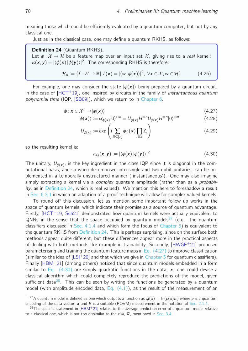
70 4. Preliminaries III: Quantum machine learning
meaning those which could be efficiently evaluated by a quantum computer, but not by anyclassical one.
Just as in the classical case, one may define a quantum RKHS, as follows:
Definition 24 (Quantum RKHS).Let φ : X → H be a feature map over an input set X , giving rise to a real kernel:κ(x ,y) = |〈φ(x) |φ(y)〉|2. The corresponding RKHS is therefore:
Hκ := f : X → R| f (x) = |〈w |φ(x)〉|2, ∀x ∈ X ,w ∈H (4.26)
For example, one may consider the state |φ(x)〉 being prepared by a quantum circuit,in the case of [HCT+19], one inspired by circuits in the family of instantaneous quantumpolynomial time (IQP, [SB09]), which we return to in Chapter 6.
φ : x ∈ X n→|φ(x)〉 (4.27)
|φ(x)〉 := Uφ(x)|0〉⊗n = Uφ(x)H⊗nUφ(x)H
⊗n|0〉⊗n (4.28)
Uφ(x) := exp
(i ∑S⊆[n]
φS(x) ∏i∈S
Zi
)(4.29)
so the resulting kernel is:κQ(x ,y) := |〈φ(x) |φ(y)〉|2 (4.30)
The unitary, Uφ(x), is the key ingredient in the class IQP since it is diagonal in the com-putational basis, and so when decomposed into single and two qubit unitaries, can be im-plemented in a temporally unstructured manner (‘instantaneous’). One may also imaginesimply extracting a kernel via a complex quantum amplitude (rather than as a probabil-ity, as in Definition 24, which is real valued). We mention this here to foreshadow a resultin Sec. 6.3.1 in which an adaption of a proof technique will allow for complex valued kernels.
To round off this discussion, let us mention some important follow up works in thespace of quantum kernels, which indicate their promise as a source of quantum advantage.Firstly, [HCT+19, Sch21] demonstrated how quantum kernels were actually equivalent toQNNs in the sense that the space occupied by quantum models27 (e.g. the quantumclassifiers discussed in Sec. 4.1.4 and which form the focus of Chapter 5) is equivalent tothe quantum RKHS from Definition 24. This is perhaps surprising, since on the surface bothmethods appear quite different, but these differences appear more in the practical aspectsof dealing with both methods, for example in trainability. Secondly, [HWGF+21] proposedparameterising and training the quantum feature maps in Eq. (4.27) to improve classification(similar to the idea of [LSI+20] and that which we give in Chapter 5 for quantum classifiers).Finally [HBM+21] (among others) noticed that since quantum models embedded in a formsimilar to Eq. (4.30) are simply quadratic functions in the data, x , one could devise aclassical algorithm which could completely reproduce the predictions of the model, givensufficient data28. This can be seen by writing the functions be generated by a quantummodel (with amplitude encoded data, Eq. (4.1)), as the result of the measurement of an
27A quantum model is defined as one which outputs a function as fθ(x) = Tr (ρ(x)E) where ρ is a quantumencoding of the data vector, x and E is a suitable (POVM) measurement in the notation of Sec. 2.1.4.
28The specific statement in [HBM+21] relates to the average prediction error of a quantum model relativeto a classical one, which is not too dissimilar to the risk, R, mentioned in Sec. 3.4.

4.3. Quantum learning theory 71
observable as:
f (x) = Tr (ρ(x)E) =
(n
∑k=1
xk∗〈k |
)U†OU
(n
∑l=1
x l |l〉
)=
n
∑k=1
n
∑l=1
Bklxk∗x l (4.31)
which is simply a quadratic function in the data point with n2 coefficients and can be fitclassically using n2/ε data examples (as shown in [HBM+21])
This indicates that even though a kernel or quantum model may be intractable to com-pute exactly, it may not actually outperform a classical model on the task of interest (atrue quantum advantage in machine learning). However, one may expect that classical in-tractability is at least a prerequisite for quantum advantage, since if one has the ability toefficiently simulate the model, solving the learning task is also classically possible. We makea similar observation in the context of generative modelling in Chapter 6.
In light of this, [HBM+21] proposes a projected quantum kernel which is a functionof the reduced density matrices of two encoded feature maps. With such a kernel, anda measure known as the geometric difference, [HBM+21] was able to also demonstrate asizeable outperformance over a comparable classical machine learning algorithm.
4.3 Quantum learning theory
To round off this chapter, let us circle back to the discussion of classical learning theorypresented in Sec. 3.6. The field of quantum learning theory is almost as old as quantumcomputation itself, having been initiated by [BJ95]. In this work, the quantum randomexample oracle (QPEX) was introduced (recall Definition 18), which instead of outputtinga single labelled example when queried, produces a superposition of all possible labelledexamples:
Definition 25 (Quantum random access oracle [BJ95]).A quantum random access oracle, QPEX, when queried outputs a quantum state ofthe following form:
QPEX→ |ψ〉 := ∑x
√D(x)|x , f (x)〉 (4.32)
The work of [BJ95] demonstrated how, when given quantum access to such examples,certain learning problems (for example the problem disjunctive normal form (DNF) couldbe solved with exponentially fewer queries than classically possible. There is an importantcaveat however, in that this is achievable relative to a specific distribution (the uniformdistribution) and in general it is known that such exponential reductions are not possible.The result of [SG04] demonstrates how if there exists a quantum learning algorithm fora given problem, then there also exists a classical algorithm for the same problem, whichrequires at most polynomially more samples than its quantum counterpart29. So, we haveanother no free lunch for quantum learning theory. This is perhaps not so surprising - wealso only have exponential speedups with a handful of quantum algorithms, so why shouldthere be any difference with learning theory problems?
To complement [SG04], the work of [AdW17b] proved the following theorem, the quan-tum analogue Theorem 3:
29The result of [AdW17b] subsequently proved optimal sample complexity bounds for quantum learning.

72 4. Preliminaries III: Quantum machine learning
Theorem 4: ([AdW17b, AdW17a])Let F be a concept class with VCdim(F). Then, for every δ ∈
(0, 1
2
)and ε ∈
(0, 1
20
):
M = Ω
(VCdim(F)−1
ε+
log(1/δ)
ε
)(4.33)
examples are necessary and sufficient for an (ε,δ)-PAC learner for F .
This theorem illustrates that quantum provides no sample complexity advantage whenwe require learning to be with respect to every distribution. In the last few years, there havebeen a flurry of results in quantum learning theory, for example, [AS05, Kot14, AGS19,ACL+20, AGY20, AGY20] and perhaps most excitingly, the theoretical demonstration of anexponential speedup using support vector machines [LAT21]. The latter result is somewhatcontrived and uses an engineered kernel in the spirit of Sec. 4.2 based on the discretelogarithm. As such it is not as ‘natural’ as one might like. However it is a very promisingstart. In Chapter 6, we will discuss a work which proved a similar result in the distributionlearning framework. For an excellent overview of topics in quantum learning theory, weencourage the reader to see [AdW17a].

5
Robust data encodings for quantumclassifiers
The Authors: “. . . when today’s intelligent systems fail, they often fail spec-tacularly disgracefully without warning or explanation, leaving a user staring at anincoherent output, wondering why the system did what it did.”
– Grad-CAM ([SCD+20])
5.1 Introduction
In Sec. 3.3.1 we introduced the problem of classification, one of the most common problemsfor which classical neural networks are deployed. In Sec. 4.1.4, we then described a notion ofa quantum classifier, one based on a PQC which required data vectors, x , to be encoded intoquantum states after which a label is extracted via a single qubit measurement. However,everything in this previous discussion assumed access to a perfect quantum computer - onein which data uploading and processing is achieved perfectly, with no errors in the process.Of course, this assumption is not valid in the NISQ regime.
In Sec. 2.1.5, we introduced some example noise models which are present on NISQdevices, and also discussed the overheads required to implement ‘coherent’ or ‘fault-tolerant’quantum algorithms, which put them out of the reach of current devices. We also touchedon the overhead required to detect and correct errors, which are vital subroutines. Giventhis, the main question we ask in this chapter is the following. Given an application specificmindset, is it possible to gain any natural noise tolerance (or robustness) for free. Theapplication we have in mind is the variational quantum classifier, and we shall see in thischapter how even posing this question raises interesting ideas.
As a spoiler, the answer we give to this question is: yes (but we may need to be slightlypathological in our model designs).
Before we begin, let us outline the structure of the chapter. We begin by presentinga more formal definition of the variational quantum classifier we consider in Sec. 5.2. Weelaborate on the definitions and examples of data encodings from Sec. 4.1.4. After this, wepresent analytic results and proofs for robustness in Sec. 5.3. We begin by showing that dif-ferent encodings lead to different classes of learnable decision boundaries, then characterisethe set of robust points for example quantum channels (those presented in Sec. 2.1.5). Westate and prove robustness results, and discuss the existence of robust encodings. Finally,
73

74 5. Robust data encodings for quantum classifiers
we prove a lower bound on the number of robust points in terms of fidelities between noisyand ideal states. Lastly, we include several numerical results in Sec. 5.4 that reinforce andextend our findings. Finally, we conclude this chapter with some musings in Sec. 5.5.
5.2 Quantum classifiers
Let us begin by defining specifically what we mean by a quantum classifier. We also inthis chapter deal only with binary classifiers, where the label takes only two possible values,y i ∈ 0,1 for a corresponding datapoint (or feature vector), x i ∈ X 1. Let M denote thenumber of such datapoints in a dataset.
Figure 5.1: A common architecture for a binary quantum classifier that we study in this work. Thegeneral circuit structure is shown in (a) and the structure for a single qubit is highlighted in (b). In both, afeature vector x is encoded into a quantum state ρx via a “state preparation” unitary Sx . The encoded stateρx then evolves to UρxU† =: ρx where U(α) is a unitary ansatz with trainable parameters α. A single qubitof the evolved state ρx is measured to yield a predicted label y for the vector x .
Given this data, the goal (as discussed in Sec. 3.3.1) is to output a rule f : X → 0,1which accurately classifies the data and can predict the labels of unseen data.
For quantum classification, outputting information (predictions) can be done in a rel-atively straightforward manner. As several authors have noted [FN18, SBSW20, SP18,GBC+18, PSCLGFL20], it is natural to use the measurement outcome of a single qubit,which produces a binary outcome, as a class prediction2. We adopt this strategy in thischapter.
Informally, we define a (binary) quantum classifier as a procedure for encoding data intoa quantum circuit, processing it through trainable PQC, and outputting a (binary) predictedlabel. Given a feature vector x ∈X , a concise description of such a classifier can be writtenas:
1In practice, we typically have X = RN , but other sets — e.g., X = ZN or X ∈ ZN2 — are possible, so wewrite X for generality.
2An alternative strategy could be to use the parity (±1)of outcome measurements from all qubits, asproposed by [ASZ+21]. However, this is a global property and therefore may suffer from barren plateauproblems as introduced in Sec. 4.1.3

5.2. Quantum classifiers 75
Encoding
x 7→ ρx (5.1)
Processing
ρx 7→ ρx (5.2)
Prediction
ρx 7→ y [ρx ] (5.3)
Several remarks are in order. First, a given data point x in the training set is encodedin a quantum state ρx ∈ Sn via a state preparation unitary Sx (introduced in Sec. 4.1.4 andwe elaborate in Sec. 5.2.1). We remark that each (unique) x in the training set leads to a(unique) Sx , so the state preparation unitary can be considered a parameterized family ofunitary ansätze.
For the processing step Eq. (5.2), several ansatz architectures have been proposed inthe literature, including quantum convolutional neural networks (mentioned in Sec. 4.1.4)[CCL19, HSPC20], strongly entangling ansätze [SBSW20], and more [SS16, GBC+18]. Inthis chapter, we allow for a general unitary evolution U(α) such that:
ρx = U(α)ρxU†(α) (5.4)
We remark that some classifier ansätze involve intermediate measurements and conditionalprocessing (notably [CCL19]) and so do not immediately fit into Eq. (5.4). Our techniquesfor showing robustness could be naturally extended to such architectures, however, and sowe consider Eq. (5.4) as a simple yet general model. We primarily focus on data encodingsand their properties in this chapter, and not on other VQA features such as the choice ofcost function. For this reason we often suppress the trainable parameters α and write Ufor U(α).
Finally, the remaining step is to extract information from the state ρx to obtain apredicted label. As mentioned, a natural method for doing this is to measure a single qubitwhich yields a binary outcome 0 or 1 taken as the predicted label y . Since measurementsare probabilistic, we measure Nm times and take a “majority vote.” That is, if 0 is measuredN0 times and N0 > Nm/2, we take 0 as the class prediction, else 1. Generalising the finitestatistics3, this condition can be expressed analytically as
y [ρx ] =
0 if Tr[Πc0ρx ]> 1
2
1 otherwise, Πc0 := |0〉〈0 |c ≡ |0〉〈0|c ⊗1c (5.5)
is the projector onto the ground state of the classification qubit, labelled c , and the remainingqubits are labelled c . For brevity we often omit these labels when it is clear from context.Throughout this chapter, we use y for predicted labels and y for true labels, and we referto Eq. (5.5) as the decision rule for the classifier. Eq. (5.5) is not the only choice for sucha decision rule. In particular, one could choose a different “weight” λ such that y = 0 ifTr[Π0ρx ]> λ as in [PSCLGFL20], add a bias to the classifier as in [SBSW20], or measurethe classification qubit in a different basis. The latter shall be an example of a techniqueto gain robustness to certain noise models later. Let us also remark that this decisionboundary is ‘harsh’, in the sense that it does not discriminate, in principle, between pointswhich have only Tr[Πc0ρx ] = 1/2 +ε versus those which have Tr[Πc0ρx ] = 1−ε. As such, onecould also introduce a sequence of soft decision rules by defining the model based on the
3We discuss details arising from finite statistics in Sec. 5.3.4. The results we prove can be easily modifiedto incorporate finite statistics as shown in this section, but they are simpler to state in terms of probabilities.

76 5. Robust data encodings for quantum classifiers
distance of the single qubit probability4 to 1/2. Such decision rules also allow the classifier toexpress a ‘confidence’ in its choice for a given label. Our techniques for showing robustness(Sec. 5.3.3) could be easily adapted for such alternate decision boundaries.
The preceding discussion is summarised with the following formalisation:
Definition 26 ((Variational) quantum classifier).A (binary) variational quantum classifier consists of three functions:
(i) An encoding function:
E : X → Sn, E(x) = ρx (5.6)
(ii) A function which evolves the state (possibly including ancillary qubits and/ormeasurement):
U : C2n×2n → C2m×2m , U(ρx) = ρx (5.7)
(iii) A decision rule:y : C2m×2m →0,1 (5.8)
Note that we have not included training data or a cost function in this definition, so aquantum classifier can be considered a hypothesis family. We can distinguish between thehypothesis family and the trained model — in which optimisation has been performed tominimise a cost function over a specified training data set — by referring to the latter as therealised quantum classifier if it is not clear from context. Let us now concentrate our focusto the primary object of interest for the remainder of this chapter, step (i) in Definition 26,the data encoding strategy.
5.2.1 Data encodings
As discussed in Sec. 4.1.4, a data encoding can be thought of as “loading” a data point x ∈Xfrom memory into a quantum state so that it can be processed by a classifier. To presentthe work of this chapter, we primarily focus on the example of a single qubit classifier. Thisis highly illustrative and allows us to visualise some nice features of the model. We will alsofocus on variations of the ‘qubit’ encoding in Definition 23, i.e. data encodings whose statepreparation unitary is of the form:
Sφ(x) =n⊗i=1
Sφi (x). (5.9)
However, we remark that some of the results presented towards the end of the chapter doin fact generalise to multi-qubit classifiers.
As a first step, let us generalise the product encoding of Eq. (4.20) to reduce thenumber of qubits required by a factor of two. We do so by exploiting the relative phasedegree of freedom in a single qubit and define a ‘dense angle’5:
4In practice, this is easily achieved by defining the decision rule based on the positivity, or negativity ofthe expectation value of Z on the classification qubit, 〈Zc〉ρx . We deal with the probabilities rather thanexpectation values for simplicity, but the results could be extended in a straightforward manner.
5The qubit encoding in Eq. (4.20) is sometimes referred to as an ‘angle’ encoding. Here we make it‘dense’ by utilising both degrees of freedom in a single qubit.

5.2. Quantum classifiers 77
Figure 5.2: A visual representation of data encoding Eq. (5.6) for a single qubit. On the left is shown aset of randomly generated points x i ,y iMi=1 normalised to lie within the unit square, (x i = [x i1,x
i2]T ), separated
by a true decision boundary shown by the dashed black line. A data encoding maps each x i ∈ R2 to a pointon the Bloch sphere ρx i ∈ C2. The dashed black line on the Bloch sphere shows the initial decision boundaryof the quantum classifier. During the training phase, unitary parameters are adjusted to rotate the dashedblack line to correctly classify as many training points as possible. Different data encodings lead to differentlearnable decision boundaries and different robustness properties.
Definition 27. [Dense angle encoding]Given a feature vector x = [x1, ...,xN ]T ∈ RN , the dense angle encoding maps x 7→EDAE(x) as:
|φ(x)〉 :=
dN/2e⊗i=1
cos(πx2i−1)|0〉+e2πix2i sin(πx2i−1)|1〉 (5.10)
For some of our analytic and numerical results, we highlight the dense angle encodingfor two-dimensional data x ∈ R2 with a single qubit given by
|φ(x)〉DAE := cos(πx1)|0〉+e2πix2 sin(πx1)|1〉 (5.11)
which has density matrix
ρx =
[cos2πx1 e−2πix2 cosπx1 sinπx1
e2πix2 cosπx1 sinπx1 sin2πx1
]
Although the angle encoding in Eq. (4.20) and dense angle encoding in Eq. (5.10)use sinuosoids and exponentials, there is nothing special about these functions (other than,perhaps, they appear in common parameterisations of qubits and unitary matrices [NC10]).We can easily abstract these to a general class of qubit encodings which use arbitraryfunctions6.
6In fact, we already did this when introducing data encodings in Sec. 4.1.4. The main difference here is adefinition with approximately half the required number of qubits.

78 5. Robust data encodings for quantum classifiers
Definition 28. [General qubit encoding]Given a feature vector x = [x1, ...,xN ]T ∈ RN , the general qubit encoding maps x 7→EGQE(x) as:
|φ(x)〉GQE :=
dN/2e⊗i=1
fi(x2i−1,x2i)|0〉+gi(x2i−1,x2i)|1〉 (5.12)
where f ,g : R×R→ C are such that |fi |2 + |gi |2 = 1 ∀i .
We remark that a similar type of generalisation was used in [PSCLGFL20] with a singlequbit classifier that allowed for repeated application of an arbitrary state preparation unitary.However, a key difference in our definition is that care needs to be taken to avoid informationloss in the encoding - a single qubit only has two degrees of freedom, while a general SU(2)
unitary has three. Therefore, while it is technically possible to use three sequential rotationgates as an encoding unitary, each with a single feature encoded in the rotation angle, thisis perhaps not advisable. While this strategy would reduce the number of qubits requiredby a factor of 3 over the product encoding of Eq. (5.9)), information in the feature vectorswill be lost since the input state is usually fixed at |0〉⊗n.
We can also similarly generalise the amplitude encoding to allow for parameterisationsof features (amplitudes).
Definition 29 (Generalised amplitude encoding).For x ∈ CN , the generalised amplitude encoding maps x 7→ EGAE
φ=fiNi=1
as:
EGAEφ=fiNi=1
: x ∈ CN →N
∑i=1
fi(x)|i〉, ∑i
|fi |2 = 1, ∀i (5.13)
The functions fi could only act on the i th feature, e.g. fi(x) = sinxi , or could be morecomplicated functions of several (or all) features. Note, we are not commenting on theefficiency of preparing such a state here.
Thus far, we have formally defined a data encoding Eq. (5.12) and its role in a quantumclassifier (Definition 26), and we have given several examples. While we have discusseddifferent properties of state preparation circuits which implement data encodings (depth,overhead, etc.), we have not yet discussed the two main properties of data encodings weconsider in this chapter: learnability and robustness. By learnability, we mean the expressivepower [RPK+17] of a given hypothesis family in its ability to find a set of parameters suchthat the realised quantum classifier can (optimally) separate the data classes. In otherwords, learnability measures the extent to which the quantum classifier can represent certainfunctions. We show in Sec. 5.3.1 that different data encodings lead to different classes oflearnable decision boundaries. For robustness, we show that different data encodings leadto different sets of robust points (to be defined) in Sec. 5.3.2 — Sec. 5.3.5. As a teaserfor the statement made in the introduction of this chapter, we find that encodings alwaysexist which satisfy our robustness definitions, but these may come at the expense of thelearnability of our model, and hence are pathological.
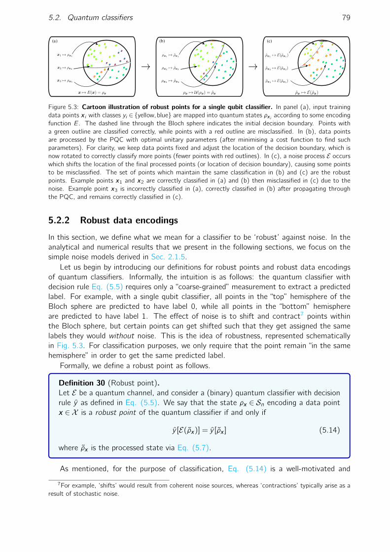
5.2. Quantum classifiers 79
(b)(a) (c)
Figure 5.3: Cartoon illustration of robust points for a single qubit classifier. In panel (a), input trainingdata points x i with classes yi ∈ yellow,blue are mapped into quantum states ρx i according to some encodingfunction E. The dashed line through the Bloch sphere indicates the initial decision boundary. Points witha green outline are classified correctly, while points with a red outline are misclassified. In (b), data pointsare processed by the PQC with optimal unitary parameters (after minimising a cost function to find suchparameters). For clarity, we keep data points fixed and adjust the location of the decision boundary, which isnow rotated to correctly classify more points (fewer points with red outlines). In (c), a noise process E occurswhich shifts the location of the final processed points (or location of decision boundary), causing some pointsto be misclassified. The set of points which maintain the same classification in (b) and (c) are the robustpoints. Example points x1 and x2 are correctly classified in (a) and (b) then misclassified in (c) due to thenoise. Example point x3 is incorrectly classified in (a), correctly classified in (b) after propagating throughthe PQC, and remains correctly classified in (c).
5.2.2 Robust data encodings
In this section, we define what we mean for a classifier to be ‘robust’ against noise. In theanalytical and numerical results that we present in the following sections, we focus on thesimple noise models derived in Sec. 2.1.5.
Let us begin by introducing our definitions for robust points and robust data encodingsof quantum classifiers. Informally, the intuition is as follows: the quantum classifier withdecision rule Eq. (5.5) requires only a “coarse-grained” measurement to extract a predictedlabel. For example, with a single qubit classifier, all points in the “top” hemisphere of theBloch sphere are predicted to have label 0, while all points in the “bottom” hemisphereare predicted to have label 1. The effect of noise is to shift and contract7 points withinthe Bloch sphere, but certain points can get shifted such that they get assigned the samelabels they would without noise. This is the idea of robustness, represented schematicallyin Fig. 5.3. For classification purposes, we only require that the point remain “in the samehemisphere” in order to get the same predicted label.
Formally, we define a robust point as follows.
Definition 30 (Robust point).Let E be a quantum channel, and consider a (binary) quantum classifier with decisionrule y as defined in Eq. (5.5). We say that the state ρx ∈ Sn encoding a data pointx ∈ X is a robust point of the quantum classifier if and only if
y [E(ρx)] = y [ρx ] (5.14)
where ρx is the processed state via Eq. (5.7).
As mentioned, for the purpose of classification, Eq. (5.14) is a well-motivated and
7For example, ‘shifts’ would result from coherent noise sources, whereas ‘contractions’ typically arise as aresult of stochastic noise.

80 5. Robust data encodings for quantum classifiers
reasonable definition of robustness. We remark that Eq. (5.14) is expressed in termsof probability; in practice, additional measurements may be required to reliably determinerobustness. We discuss this point further in Sec. 5.3.4.
Further, we note that Eq. (5.14) assumes that noise occurs only after the evolutionρx 7→ ρx . While this may be a useful theoretical assumption, in practice noise happensthroughout a quantum circuit. We can therefore consider robustness for an ideal dataencoding as in Definition 30, or for a noisy data encoding in which some noise process E1
occurs after encoding and another noise process E2 occurs after evolution:
y [E2(U(E1(ρx)))] = y [ρx ] (5.15)
For our results, we primarily consider Eq. (5.14), although we show robustness for Eq.(5.15) in some cases.
Robust points (Eq. (5.14)) are related but not equivalent to (density operator) fixedpoints of a quantum channel, and can be considered an application-specific generalisationof fixed points. In Sec. 5.3.2, we characterise the set of robust points for example channels,and in Sec. 5.3.5 we use this connection to prove the existence of robust data encodings.
For classification, we are concerned with not just one data point, but rather a set ofpoints (e.g., the set X or training set Eq. (3.5)). We therefore define the set of robustpoints, or robust set, in the following natural way.
Definition 31 (Robust set).Consider a (binary) quantum classifier with encoding E : X → Sn and decision rule yas defined in Eq. (5.5). Let E be a quantum channel. The set of robust points, orsimply robust set, is
R(E ,E, y) := x ∈ X : y [E(ρx)] = y [ρx ] (5.16)
where ρx is the processed state via Eq. (5.7) and ρx = E(x).
While the robust set generally depends on the encoding E, there are cases in whichR is independent of E. In this scenario, we say all encodings are robust to this channel.Otherwise, the size of the robust set (i.e., number of robust points) can vary based on theencoding, and we distinguish between two cases. If the robust set is the set of all possiblepoints, we say that the encoding is completely robust to the given noise channel.
Definition 32 (Completely robust data encoding).Consider a (binary) quantum classifier with encoding E and decision rule y as definedin Eq. (5.5). Let x ∈ X and let E be a quantum channel. We say that E is acompletely robust data encoding for the quantum classifier if and only if
R(E ,E, y) = X (5.17)
We note that in practice (e.g. for numerical results), complete robustness is determinedrelative to the training set Eq. (3.5). That is, we empirically observe that E is a completelyrobust data encoding if and only if
R(E ,E, y) = x iMi=1 (5.18)

5.3. Analytic results 81
Complete robustness can be a strong condition, so we also consider a partially robustdata encoding, defined as follows.
Definition 33 (Partially robust data encoding).Consider a (binary) quantum classifier with encoding E and decision rule y as definedin Eq. (5.5). Let x ∈X and let E be a quantum channel. We say that E is a partiallyrobust data encoding for the quantum classifier if and only if
R(E ,E, y)( X (5.19)
Similar to complete robustness, partial robustness is determined in practice relative tothe training set. For 0≤ δ ≤ 1, we say that E is a δ-robust data encoding if and only if
|R(E ,E, y)|= δM (5.20)
where | · | denotes cardinality so that |R(E ,E, y)| ∈ [M].
5.3 Analytic results
Using the definitions from Sec. 2.1.5, we now state and prove results about data encodings8.First, we show that different encodings lead to different classes of decision boundaries inSec. 5.3.1. Next, we characterise the set of robust points for example quantum channelsin Sec. 5.3.2. In Sec. 5.3.3, we prove several robustness results for different quantumchannels, and in Sec. 5.3.5 we discuss the existence of robust encodings as well as anobserved tradeoff between learnability and robustness. Finally, in Sec. 5.3.6, we prove anupper bound on the number of robust points in terms of fidelities between noisy and noiselessstates.
Before diving into these results, let us first derive some useful identities for a single qubitclassifier. Let ρ be a single qubit state with matrix elements ρi j , i.e.
ρ :=
(ρ00 ρ01
ρ10 ρ11
)Then we have:
XρX =
(ρ11 ρ10
ρ01 ρ00
)YρY =
(ρ11 −ρ10
−ρ01 ρ00
)ZρZ =
(ρ00 −ρ01
−ρ10 ρ11
)Next, defining the projectors Π0 := |0〉〈0 | and Π1 := |1〉〈1 |, one can show
Tr[Π0XρX] = Tr[Π1ρ], Tr[Π0Y ρY] = Tr[Π1ρ] Tr[Π0ZρZ] = Tr[Π0ρ]
For any Hermitian matrix A= [Ai j ] and any unitary matrix U = [Ui j ], we have
Tr[Π0UAU†] = |U00|2A00 + 2<[U∗00U01A10] + |U01|2A11. (5.21)
Similarly, one can show that
Tr[Π1UAU†] = |U10|2A00 + 2<[U∗11U10A01] + |U11|2A11. (5.22)
8In actual fact, our results generally apply to the entire model as a whole, not just the data encoding.

82 5. Robust data encodings for quantum classifiers
If we further assume the single qubit unitary, U(α), has the decomposition: Rz(2α1)Ry (2α2)Rz(2α3)
(up to a global phase) [NC10], we get:
U(α) =
(ei(−α1−α3) cosα2 −ei(−α1+α3) sinα2
ei(α1−α3) sinα2 ei(α1+α3) cosα2
)(5.23)
Therefore, we get the various terms in Eq. (5.21), Eq. (5.22) t be:
|U00|2 = cos2(α2), |U01|2 = |U10|2 = sin2(α2), |U11|2 = cos2(α2)
U∗00U01 =−ei2α3 cos(α2)sin(α2) =−1
2e2iα2 sin(2α2)
U∗11U10 = e−i2α3 cos(α2)sin(α2) =1
2e−2iα3 sin(2α2)
So the conditions become:
Tr[Π0UAU†] = |U00|2A00 + 2<[U∗00U01A10] + |U01|2A11
= cos2 (α2)A00 + sin2 (α2)A11−<[e2iα3 sin(α2)A10]
Tr[Π1UAU†] = |U10|2A00 + 2<[U∗11U10A01] + |U11|2A11
= sin2 (α2)A00 + cos2 (α2)A11 +<[e−2iα3 sin(2α2)A01]
5.3.1 Classes of learnable decision boundaries
In Sec. 4.1 and Sec. 5.2.1 we introduced several data encodings and discussed differencesin the state preparation circuits which realise them. Here, we show that different encodingslead to different sets of decision boundaries for the quantum classifier, thereby demonstratingthat the success of the quantum classifier in Definition 26 depends crucially on the dataencoding Eq. (5.12)9.
The decision boundary according to the decision rule Eq. (5.5) is implicitly defined by
Tr[Π0ρx ] =1
2(5.24)
Consider a single qubit encoding Eq. (5.12) so that:
ρx =
(f (x1,x2)2 f (x1,x2)g(x1,x2)∗
f (x1,x2)g(x1,x2) |g(x1,x2)|2)
where we assumed without loss of generality that f is real valued. Let the unitary U besuch that ρx = UρxU
† and has matrix elements Ui j . Then, one can write the decisionboundary Eq. (5.24) as (see Eq. (5.21))
|U00|2f 2 + 2<[U∗00U01f g] + |U01|2|g|2 =1
2(5.25)
where we have let f := f (x1,x2) and g := g(x1,x2) for brevity. Eq. (5.25) implicitly definesthe decision boundary in terms of the data encoding f and g. The unitary matrix elementsUi j then define the hypothesis family.
9This fundamental importance of the data encoding in quantum classifiers has also been observed andreinforced in previous and subsequent work to ours [LSI+20, GVT20, SSM21].

5.3. Analytic results 83
Eq. (5.25) can be solved numerically for different encodings, and we do so in Sec. 5.4.1(Fig. 5.6) to visualise decision boundaries for single qubit classifiers. At present, we canproceed further analytically with a few inconsequential assumptions to simplify the equations.
For the amplitude encoding, we have f (x1,x2) = x1 and g(x1,x2) = x2. Suppose forsimplicity that matrix elements U00 =: a and U01 =: b are real. Then, Eq. (5.25) can bewritten
(ax1 +bx2)2 =1
2(5.26)
which defines a line x2 = x2(x1) with slope −a/b and intercept 1/√
2b. Thus, a single qubitclassifier in Definition 26 which uses the amplitude encoding Eq. (4.1) can learn decisionboundaries that are straight lines.
Now consider the dense angle encoding Eq. (5.10) on a single qubit, for which f (x1,x2) =
cos(πx1) and g(x1,x2) = e2πix2 sin(πx1). Supposing again that matrix elements U00 ≡ a andU01 ≡ b are real, we can write Eq. (5.25) as
a2 cos2πx1 + 2abcosπx1 sinπx1 cos2πx2 +b2 sin2πx1 =1
2(5.27)
This can be rearranged to
cos2πx2 =1−2a2 + (2a2−2b2)sin2πx1
ab sin2πx1(5.28)
which defines a class of sinusoidal functions x2 = x2(x1) (see Fig. 5.6 in Sec. 5.4.1).The different decision boundaries defined by Eq. (5.26) and Eq. (5.28) emphasise the
effect that encoding has on learnability. A realised classifier may have poor performancedue to its encoding, and switching the encoding may lead to better results. We note that asimilar phenomenon occurs in classical machine learning — a standard example being that adot product kernel cannot separate data on a spiral, but a Gaussian kernel can. It may notbe clear a priori what encoding to use (similarly in classical machine learning with kernels),but different properties of the data may lead to educated guesses. We note that [LSI+20]consider training over hyperparameters to find good encodings, and we propose a similaridea in Sec. 5.4.3 to find good robust encodings.
5.3.2 Characterisation of robust points
Given the model of a classifier, and the definitions of our noise channels we can begin todiscuss our robustness results against these channels. Intuitively, for a given noise channelwe wish to characterise the set of robust points (Definition 31). If we then know whatconditions our classifier will be deployed in (meaning the noise model), we can then buildthe classifier to encode datapoints into this robust set. As a result, these points will beprotected. As a first step, we look instead at the fixed points of a quantum noise channelE , defined as the states ρ ∈ Sn which obey the following:
E(ρ) = ρ (5.29)
To proceed, we will first use some toy examples to build intuition and demonstrate the re-lationship between robust points and fixed points. In Sec. 5.3.5, we formalise this intuition.
84 5. Robust data encodings for quantum classifiers
We remark that the characterisations similar to the ones in this Section may be of inde-pendent interest from a purely theoretical perspective, as robust points can be considereda type of generalised fixed point, or symmetry, of quantum channels.
The pure states which are fixed points of the dephasing channel Eq. (2.40) are Π0 :=
|0〉〈0| and Π1 := |1〉〈1|, andρ= aΠ0 +bΠ1 (5.30)
with a+ b = 1 is the general mixed-state density operator fixed point. In contrast, let usnow consider the robust points of the same dephasing channel, which satisfy
y [Edephp (ρ)] = y [ρ] (5.31)
instead of Eq. (5.29). Certainly the state in Eq. (5.30) will satisfy Eq. (5.31) — i.e.,any fixed point is a robust point — but the set of robust points may be strictly larger. Tocompletely characterise the robust set, we seek the set of ρ ∈ S2 such that
Tr[Π0ρ]> 1/2 =⇒ Tr[Π0Edephp (ρ)]> 1/2 (5.32)
andTr[Π0ρ]< 1/2 =⇒ Tr[Π0Edephp (ρ)]< 1/2. (5.33)
Using the simple properties of the trace and Pauli matrices from the beginning of thissection, we can write
Tr[Π0Edephp (ρ)] = (1−p)Tr[Π0ρ] +pTr[Π0ZρZ] = Tr[Π0ρ].
Thus Eq. (5.32) and Eq. (5.33) are satisfied for all density operators ρ∈ S2. That is, everydata point x ∈ X is a robust point of the dephasing channel (independent of the encoding)for the quantum classifier in Definition 26.
Consider now an amplitude damping channel Eq. (2.43) with p = 1, for which the onlyfixed point is the pure state Π0. By expanding the decision rule Eq. (5.24) for a state underthe amplitude damping channel as:
Tr[Π0EADp (ρ)] = (1−p)Tr[Π0ρ] +p,
we see that a robust point σ must satisfy Tr[Π0σ] = 1. That is, the only robust point is Π0,and in this case the set of robust points is identical to the set of fixed points.
As expected from Eq. (5.14) and Eq. (5.29), these examples confirm that
F(E)⊆R(E,E , y) (5.34)
where F(E) denotes the set of fixed points of E . In Sec. 5.3.5, we use this connection togeneralise the above discussion and prove the existence of robust data encodings.

5.3. Analytic results 85
5.3.3 Robustness results
Regarding analytic results for robustness, we first demonstrate results for single qubit clas-sifiers with several channels in Sec. 5.3.3.1 and Sec. 5.3.3.2. Then, we state and prove arobustness result for multi-qubit classifiers with (global) depolarising noise in Sec. 5.3.3.3.
5.3.3.1 Single qubit classifier - Pauli noise
First, we consider when robustness can be achieved for a Pauli channel.
Theorem 5: Let EPp be a Pauli channel Eq. (2.38) and consider a quantum classifieron data from the set X . Then, for any encoding E : X → S2, we have completerobustness
R(EPp ,E, y) = X
if pX +pY 6 1/2. (Recall that p := [p1,pX ,pY ,pZ]).
Proof. The predicted label in the noisy case is identical to Eq. (5.5) with ρx replaced byEPp (ρx). That is,
y [EPp (ρx)] =
0 if Tr[Π0EPp (ρx)]> 1/2
1 otherwise.
By definition Eq. (2.38), we have
Tr[Π0EPp (ρx)] = p1Tr[Π0ρx ] +pXTr[Π0XρxX] +pY Tr[Π0YρxY] +pZTr[Π0ZρxZ] (5.35)
Using the straightforward expressions given at the start of this section, we may write Eq.(5.35) as:
Tr[Π0EPp (ρx)] = (p1 +pZ)Tr[Π0ρx ] + (pX +pY )Tr[Π1ρx ]
By resolution of the identity, 1 = Tr[ρx ] = Tr[Π0ρx ] +Tr[Π1ρx ], we come to the simplifiedexpression:
Tr[Π0EPp (ρx)] = [1−2ν]Tr[Π0ρx ] +ν
where ν := pX +pY .Suppose the noiseless classification is y = 0 so that Tr[Π0ρx ]> 1/2. Since ν 6 1/2, we
haveTr[Π0EPp (ρx)]> [1−2ν]
1
2+ν =
1
2
Hence, classification of data points with label y = 0 is robust for any encoding. Supposethe noiseless classification is y = 1 so that Tr[Π0ρx ]< 1/2. Since ν 6 1/2, we have
Tr[Π0EPp (ρx)]< [1−2ν]1
2+ν =
1
2.
Hence, classification of data points with label y = 1 is also robust for any encoding.
Returning to the condition, pX +pY 6 1/2, one can imagine a NISQ computer in whicheither pX or pY were large enough such that this condition is not satisfied. In this regard,we note two things. First, if this condition is not satisfied, then not every encoding strategywill be robust to the Pauli channel in this model. In particular, the set of robust points

86 5. Robust data encodings for quantum classifiers
will now be dependent on the encoding strategy. This is similar to the behaviour of theamplitude damping channel which we illustrate in Sec. 5.4.
Second, the requirement pX +pY 6 1/2 appears because the decision rule uses a mea-surement in the computational basis. We note that if we measure in the Hadamard basis(see Theorem 6) then we get a modified robustness condition, namely pY + pZ 6 1/2. Asimilar conclusion can be drawn from measurements in the Pauli-Y basis. These resultssuggest that device-specific encoding strategies and decision rules may be important forachieving robustness in practice on NISQ computers.
To illustrate the results of Theorem 5, we focus on the dense angle encoding (Defini-tion 27), and a dataset for which the DAE can achieve nearly 100% accuracy (specificallythe “vertical” dataset - see Sec. 5.4). We then compute the percentage which would bemisclassified as a function of and Pauli noise parameters, pX , pY . The results are seenin Fig. 5.4. We note here, that for values of pX + pY > 1/2, one has two strategies toachieve robustness. The first is to adjust the measurement basis as per the discussion ofthe previous paragraph and requires changing the model itself. Alternatively, one can applyan extra step of post processing and relabel every output ‘y = 0’ to ‘y = 1’, and vice versa.
Figure 5.4: Misclassification percentage as a result of Pauli noise with strengths pX ,pY ,pZ = 0. Asexpected, classification is robust for pX +pY < 1/2 based on Theorem 5, and a sharp transition occurs whenthis constraint is violated to give maximal misclassification. By classified ‘correctly’ in this context, we meanthe fraction of points which are classified the same with and without noise.
Three robustness results for different channels can be shown as corollaries of Theorem 5as follows.
1. By setting pX = pY = 0 in Theorem 5, it follows that R(Edephp ,E, y) =X . That is, allencodings are unconditionally robust to dephasing errors:
Corollary 1: Let Edephp be a dephasing channel Eq. (2.40), and consider aquantum classifier on data from the set X . Then, for any encoding E :X →S2,
R(Edephp ,E, y) = X
2. By setting pZ = pY = 0 and using a modified decision rule which measures in theHadamard basis, denoted z , it follows that R(EBFp ,E, z) = X . That is, all encodings

5.3. Analytic results 87
are unconditionally robust to bit-flip errors (using a modified decision rule). We firsthave the more general theorem, from which the above statement follows immediately(Π+ := |+〉〈+|):
Theorem 6: Consider a quantum classifier on data from the set X with modifieddecision rule:
z [ρx ] =
0 if Tr[Π+ρx ]> 1/2
1 otherwise(5.36)
Then, for any E : X → S2, with a Pauli channel EPp such that pY + pZ 6 1/2,we have:
R(EPp ,E, z) = X
We can now specialise Theorem 6 to the case pZ = pY = 0:
Corollary 2: Consider a quantum classifier on data from the set X with modifieddecision rule z defined in Eq. (5.36). Then, for any encoding E : X → S2,
R(EBFp ,E, z) = X .
3. By setting pX = pY = pZ = p/4 and p1 := (1−3p/4), we then have thatR(Edepop ,E, y) =
X . That is, all encodings are unconditionally robust to depolarising noise:
Corollary 3: Let Edepop be a depolarising channel Eq. (2.41), and consider aquantum classifier on data from the set X . Then, for any encoding E :X →S2:
R(Edepop ,E, y) = X
Interestingly, we remark that fact (3) holds with measurements in any basis, not just thecomputational basis. In Sec. 5.3.3.3, we generalise this result to multi-qubit classifiers andas well as to noisy data encodings Eq. (5.15).
5.3.3.2 Single qubit classifier - amplitude damping
Let us now move to amplitude damping noise, for which the robust set R depends on theencoding E. From the channel definition Eq. (2.43), it is straightforward to see that:
Tr[Π0EADp (ρx)] = Tr[Π0ρx ] +pTr[Π1ρx ] (5.37)
Suppose first that the noiseless prediction is y = 0 so that Tr[Π0ρx ]> 1/2. Then, certainlyTr[Π0EADp (ρx)]> 1/2 because p > 0 and Tr[Π1ρx ]> 0. Thus, the noisy prediction is alwaysidentical to the noiseless prediction when the noiseless prediction is y = 0. This can beunderstood intuitively because an amplitude damping channel only increases the probabilityof the ground state. Now, suppose that the noiseless prediction is y = 1. From Eq. (5.37),we require:
Tr[Π0EADp (ρx)] = Tr[Π0ρx ] +pTr[Π1ρx ]< 1/2

88 5. Robust data encodings for quantum classifiers
to achieve robustness. Using the resolution of the identity, Tr[Π1ρx ] = 1−Tr[Π0ρx ], wearrive at the condition:
Tr[Π1ρx ]>1
2(1−p)(5.38)
Let ρx be given by the general qubit encoding Eq. (5.12) so that Eq. (5.38) can be written(see Eq. (5.22))
|U10|2f 2 + 2<[U∗11U10f g∗] + |U11|2|g|2 >
1
2(1−p)
where Ui j denote the optimal unitary matrix elements. Formally, we then have:
Theorem 7: Consider a quantum classifier on data from the set X , and let EADpdenote the amplitude damping channel Eq. (2.43). Then, for any qubit encoding Edefined in Eq. (5.12) which satisfies
|U10|2f 2 + 2<[U∗11U10f g∗] + |U11|2|g|2 >
1
2(1−p), (5.39)
we haveR(EADp ,E, y) = X .
If E is not completely robust, the set of points x such that Eq. (5.39) holds definethe partially robust set.
We note that Eq. (5.39) depends on the optimal unitary U as well as the encoding E.This is expected as the final state ρx has been processed by the PQC. In practice, sincewe do not know the optimal unitary parameters a priori, it remains a question of how largethe (partially) robust set will be for a given an encoding. To address this point, we discussin Sec. 5.4.3 how training over hyperparameters in the encoding function can help find therobust region even after application of the unknown optimal unitary. Additionally, in thenext Section we discuss whether we can find an encoding which satisfies Eq. (5.39), ormore generally whether a robust encoding exists for a given channel.
Given the robustness condition Eq. (5.39) for the amplitude damping channel, it isnatural to ask whether such an encoding exists. In Sec. 5.3.5, we show the answer is yesby demonstrating there always exists a robust encoding for any trace preserving quantumoperation. This encoding may be trivial, which leads to the idea of a tradeoff betweenlearnability and robustness.
5.3.3.3 Multi-qubit classifier
We now consider global depolarising noise on a multi-qubit classifier. It turns out that anyencoding is completely robust to this channel applied at any point throughout the circuit.To clearly state the theorem, we introduce the following notation. First, let
Epi (ρ) = piρ+ (1−pi)1d
d(5.40)

5.3. Analytic results 89
be shorthand for a global depolarising channel with probability pi . (Note pi and 1−pi areintentionally reversed compared to Definition 7 to simplify the proof.) Then, let
ρ(m)x ≡
[J
∏j=1
Ui Epi
]ρx (5.41)
denote the state of the encoded point ρx after J applications of a global depolarising channeland unitary channel. For instance, J = 1 corresponds to
U1 Ep1 ρx ≡ U1(Ep1(ρx))
and m = 2 corresponds to
U2 Ep2 U1 Ep1 ρx ≡ U2(Ep2(U1(Ep1(ρx))))
We remark that Ui can denote any unitary in the circuit.With this notation, we state the theorem as follows.
Theorem 8: Consider a quantum classifier on data from the set X with decision ruley defined in Eq. (5.36). Then, for any encoding E : X → Sn,
R(EGDp ,E, y
)= X
where EGDp denotes the composition of global depolarising noise acting at any pointin the circuit — i.e. such that the final state of the classifier is given by Eq. (5.41).
To prove Theorem 8, we use the following lemma.
Lemma 1: The state in Eq. (5.41) can be written as (adapted from [SKCC20])
ρ(J)x =
J
∏j=1
piUJ · · ·U1ρxU†1 · · ·U
†J +
(1−
J
∏j=1
pj
)1d
d(5.42)
where d = 2n is the dimension of the Hilbert space.
Proof. Using the definition of the global depolarising channel Eq. (5.40), it is straightfor-ward to evaluate (with 1≡ 1d):
ρ(1)x = U1 Ep1 ρx = p1U1ρxU
†1 + (1−p1)
1
d
Thus Eq. (5.42) is true for J = 1. Assume Eq. (5.42) holds for J = k . Then, for k+ 1 wehave
ρ(k+1)x = Uk+1 Epk+1
ρ(k)x = pk+1Uk+1ρ
(k)x U
†k+1 + (1−pk+1)
1
d
The last line can be simplified to arrive at
ρ(k+1)x =
k+1
∏i=1
piUk+1 · · ·U1ρxU†1 · · ·U
†k+1 +
(1−
k+1
∏i=1
pi
)1
d(5.43)
which completes the proof.

90 5. Robust data encodings for quantum classifiers
We can now prove Theorem 8 as follows. Let l denote the total number of alternatingunitary gates with depolarising noise in the classifier circuit so that Eq. (5.42) can be written
ρ(l)x = pρx + (1− p)
1
d. (5.44)
Here, we have defined p := ∏li=1pi and noted that Ul · · ·U1ρxU
†1 · · ·U
†l = ρx is the final state
of the noiseless circuit before measuring. Eq. (5.44) is thus the final state of the noisycircuit before measuring. Then:
Tr[Π0ρ(l)x ] = pTr[Π0ρx ] +
(1− p)
2(5.45)
using Tr[Π0Id ] = 2d−1. To prove robustness, suppose that y [ρx ] = 0 so that Tr[Π0ρx ]> 1/2.Then,
Tr[Π0ρ(l)x ]>
p
2+
(1− p)
2=
1
2
so that y [ρ(l)x ] = 0. Similarly for the case y [ρx ] = 1, which completes the proof of Theorem 8.
Thus, any encoding strategy exhibits complete robustness to global depolarising noise.We remark again that our definition of robustness (Definition 30) is in terms of probabil-ities, meaning that more measurements for sampling may be required to reliably evaluaterobustness. With this remark, we note an interesting connection to explain a phenomenonobserved in recent literature: the authors of [GBC+18], found that classification accuracydecreased under the presence of depolarising noise. Theorem 8 implies this was exclusivelydue to the finite shot noise used to obtain the predicted label. We discuss errors due tofinite sampling in more detail in Sec. 5.3.4.
While global depolarising noise admits a clean robustness result for an arbitrary d-dimensional circuit, general channels can lead to complicated equations which are besthandled numerically. We include several numerical results in Sec. 5.4, and we discuss av-enues for proving more analytical results with certain classes of channels in future workin Sec. 5.5. To close the present discussion, we highlight the special case of multi-qubitclassifiers with “factorisable noise”, for which it is straightforward to apply previous resultsproved in this section.
In particular, suppose that E : Sn → Sn is a noise channel which factorises into singlequbit channels, e.g.
E = E1⊗·· ·⊗En (5.46)
where Ei : S2→S2 for i ∈ [n]. Without loss of generality, let the classification qubit be thenth qubit. Then, if the processed state of the classification qubit is robust to the channelEn, the encoded state will be robust to the entire channel E in Eq. (5.46). Specifically, wehave the following (proof in Appendix A.1.1):
Theorem 9: If E is any noise channel which factorises into a single qubit channel, anda multiqubit channel as follows:
E(ρ) = Ec(ρcx)⊗Ec(ρcx)
where WLOG Ec acts only on the classification qubit (ρcx = Trc(ρx)) after encodingand unitary evolution, and Ec acts on all other qubits arbitrarily, (ρcx = Trc(ρx)).Further assume the state meets the robust classification requirements for the singlequbit error channel Ec . Then the classifier will be robust to E .
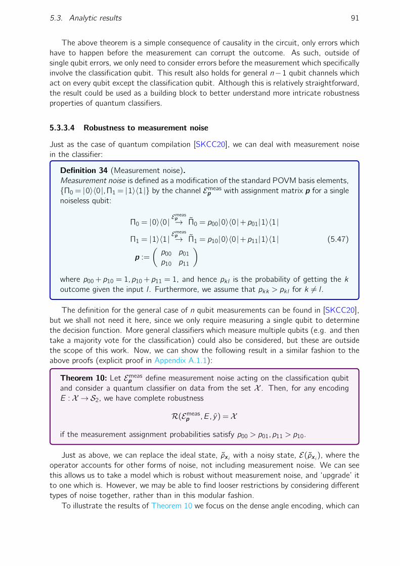
5.3. Analytic results 91
The above theorem is a simple consequence of causality in the circuit, only errors whichhave to happen before the measurement can corrupt the outcome. As such, outside ofsingle qubit errors, we only need to consider errors before the measurement which specificallyinvolve the classification qubit. This result also holds for general n−1 qubit channels whichact on every qubit except the classification qubit. Although this is relatively straightforward,the result could be used as a building block to better understand more intricate robustnessproperties of quantum classifiers.
5.3.3.4 Robustness to measurement noise
Just as the case of quantum compilation [SKCC20], we can deal with measurement noisein the classifier:
Definition 34 (Measurement noise).Measurement noise is defined as a modification of the standard POVM basis elements,Π0 = |0〉〈0|,Π1 = |1〉〈1 | by the channel Emeas
p with assignment matrix p for a singlenoiseless qubit:
Π0 = |0〉〈0 |Emeasp→ Π0 = p00|0〉〈0 |+p01|1〉〈1 |
Π1 = |1〉〈1 |Emeasp→ Π1 = p10|0〉〈0 |+p11|1〉〈1 | (5.47)
p :=
(p00 p01
p10 p11
)where p00 +p10 = 1,p10 +p11 = 1, and hence pkl is the probability of getting the koutcome given the input l . Furthermore, we assume that pkk > pkl for k 6= l .
The definition for the general case of n qubit measurements can be found in [SKCC20],but we shall not need it here, since we only require measuring a single qubit to determinethe decision function. More general classifiers which measure multiple qubits (e.g. and thentake a majority vote for the classification) could also be considered, but these are outsidethe scope of this work. Now, we can show the following result in a similar fashion to theabove proofs (explicit proof in Appendix A.1.1):
Theorem 10: Let Emeasp define measurement noise acting on the classification qubit
and consider a quantum classifier on data from the set X . Then, for any encodingE : X → S2, we have complete robustness
R(Emeasp ,E, y) = X
if the measurement assignment probabilities satisfy p00 > p01,p11 > p10.
Just as above, we can replace the ideal state, ρx i with a noisy state, E(ρx i ), where theoperator accounts for other forms of noise, not including measurement noise. We can seethis allows us to take a model which is robust without measurement noise, and ‘upgrade’ itto one which is. However, we may be able to find looser restrictions by considering differenttypes of noise together, rather than in this modular fashion.
To illustrate the results of Theorem 10 we focus on the dense angle encoding, which can
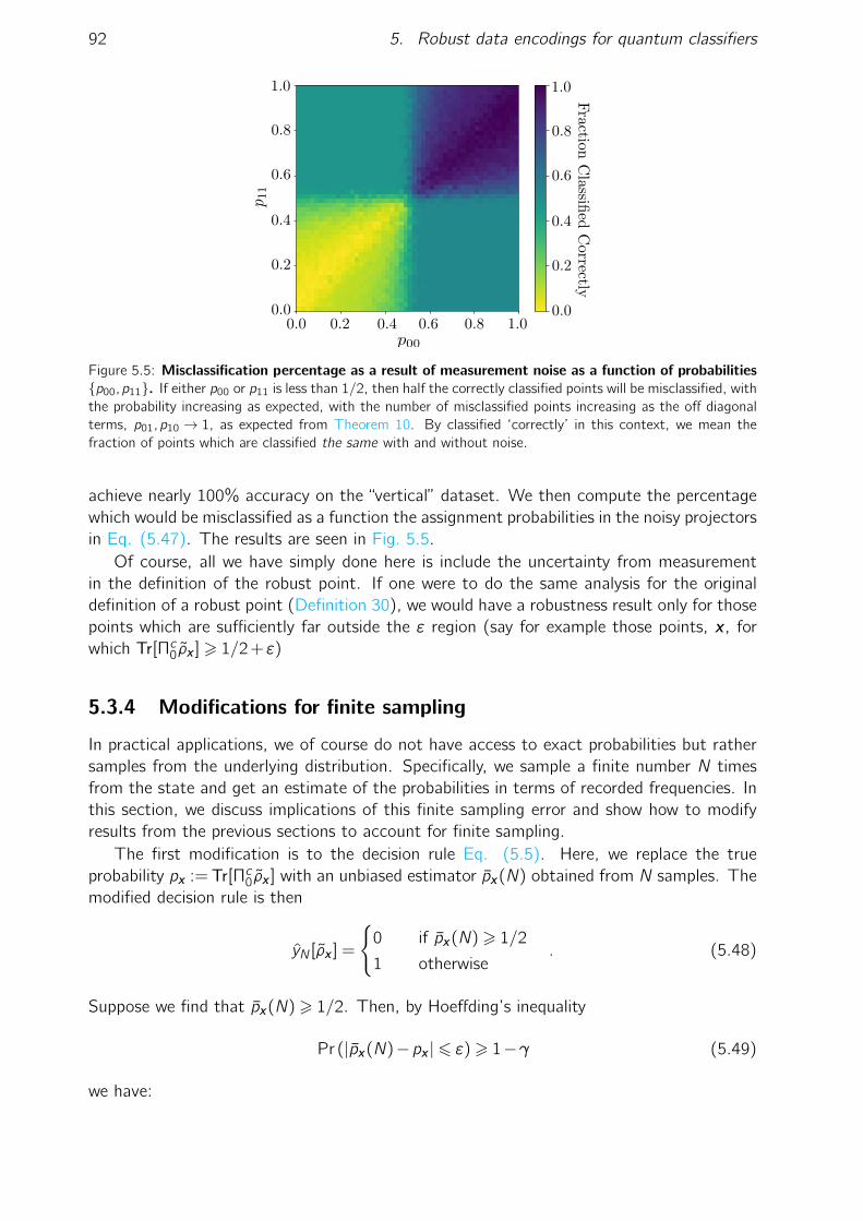
92 5. Robust data encodings for quantum classifiers
Figure 5.5: Misclassification percentage as a result of measurement noise as a function of probabilitiesp00,p11. If either p00 or p11 is less than 1/2, then half the correctly classified points will be misclassified, withthe probability increasing as expected, with the number of misclassified points increasing as the off diagonalterms, p01,p10 → 1, as expected from Theorem 10. By classified ‘correctly’ in this context, we mean thefraction of points which are classified the same with and without noise.
achieve nearly 100% accuracy on the “vertical” dataset. We then compute the percentagewhich would be misclassified as a function the assignment probabilities in the noisy projectorsin Eq. (5.47). The results are seen in Fig. 5.5.
Of course, all we have simply done here is include the uncertainty from measurementin the definition of the robust point. If one were to do the same analysis for the originaldefinition of a robust point (Definition 30), we would have a robustness result only for thosepoints which are sufficiently far outside the ε region (say for example those points, x , forwhich Tr[Πc0ρx ]> 1/2 +ε)
5.3.4 Modifications for finite sampling
In practical applications, we of course do not have access to exact probabilities but rathersamples from the underlying distribution. Specifically, we sample a finite number N timesfrom the state and get an estimate of the probabilities in terms of recorded frequencies. Inthis section, we discuss implications of this finite sampling error and show how to modifyresults from the previous sections to account for finite sampling.
The first modification is to the decision rule Eq. (5.5). Here, we replace the trueprobability px := Tr[Πc0ρx ] with an unbiased estimator px(N) obtained from N samples. Themodified decision rule is then
yN [ρx ] =
0 if px(N)> 1/2
1 otherwise. (5.48)
Suppose we find that px(N)> 1/2. Then, by Hoeffding’s inequality
Pr (|px(N)−px |6 ε)> 1−γ (5.49)
we have:

5.3. Analytic results 93
|px − px(N)|6 ε (5.50)
=⇒ −ε6 px −1
26 ε (5.51)
=⇒1
2−ε6 px 6
1
2+ε (5.52)
Therefore (taking the left hand inequality above), for any ε > 0, we know that px > 1/2−εwith probability at least 1−γ (we refer to 1−γ as the confidence) if we take:
N > Nc(ε,γ) :=1
(2ε2)log
1
γ(5.53)
samples from px . This follows since each measurement of the observable gives a Bernoullirandom variable with expectation Tr[Πc0ρx ].
We note that it is in principle #P-hard to exactly determine the predicted class labelsince points could be within any ε > 0 from the decision boundary. In practice we do notexpect this to be a limiting issue aside from pathological examples, but it is important tonote. One could introduce a penalty term into the cost function such that the distance εbetween the boundary and the closest point is maximised (as in support vector machines)to mitigate this effect.
Now, to begin the discussion of robustness in this context, we first note that clearly,finite sampling effects can be treated as a form of noise. If we consider N →∞ in Eq.(5.53), we recover the prediction of the ideal channel, yN→∞[ρx ] = y [ρx ]. Then, if N beingfinite (and fixed) is treated as a noise channel so, yN [ρx ] = y [Esamp(ρx)], all points x forwhich y [ρx ]> 1/2 +ε (assuming the label is 0) will be robust against Esamp
N .
Now, unfortunately those x ∈ X for which 1/26 y [ρx ]6 1/2 +ε may or may not be inthe robust set for the ‘finite sampling channel’, R(Esamp
N ,E, y).
Let EsampN1
be the noise channel induced by a certain number of samples, N1, suchthat a particular classifier does not have the entirety of the dataset in the robust set,R(Esamp
N1,E, y) 6= X . In order to make a classifier for which all points in the dataset are in
the robust set, we simply need to increase the number of samples to some sufficiently largevalue, N2 >N1, and we shall recover complete robustness, i.e. we have R(Esamp
N2,E, y) =X .
However, this comes at a caveat that N2 may not be a polynomial function of the problemparameters. We leave the investigation of the value N2 should be for a particular problem(as it will in general be highly problem- and dataset-dependent) to future work.
Now, in the above discussions we have taken care of the cases ‘ideal classifier → noisyclassifier’ and ‘ideal classifier → finite sampling classifier’. The final case to deal with is‘finite sampling classifier → finite sampling noisy classifier’. Coupled with the discussion ofthe number of shots required for finite-sampling robustness, this final step will allow us touplift the robustness argument for any other noise channel into the finite sampling regime,i.e. the case, ‘ideal classifier → finite sampling noisy classifier’. To do so, we present amodified definition of a robust point to account for errors due to finite sampling, specificallyone which incorporates the ε,δ parameters.

94 5. Robust data encodings for quantum classifiers
Definition 35 ((ε,γ)-Robust point).Let 0 < ε < 1/2, 0 < γ < 1, and E be a quantum channel. We say that the stateρx ∈Sn encoding a data point x ∈X is an (ε,γ)-robust point of the quantum classifierif and only if
yN [E(ρx)] = yN [ρx ] (5.54)
with confidence 1−γ. Explicitly, Eq. (5.54) gives two conditions:
Tr[Πc0ρx ]> 1/2−ε =⇒ Tr[Πc0E(ρx)]> 1/2−ε (5.55)
Tr[Πc0ρx ]< 1/2 +ε =⇒ Tr[Πc0E(ρx)]< 1/2 +ε (5.56)
with confidence 1−γ. This is achieved using N > Nc(ε,γ) := 1/(2ε2) log1/γ mea-surements in the decision rule Eq. (5.48).
Procedurally, we can think of this definition as follows. We are provided with an 0 <
ε < 1/2 which corresponds to how close to the boundary we want to be able to distinguishrobust points (the farthest we can be from the boundary is 1/2), and a 0 < γ < 1 whichcorresponds to how certain we want to be about points within this region. Every point σwhich satisfies
|Tr[σΠc0]−1/2|< ε (5.57)
is classified correctly with confidence 1−γ using at least Nc(ε,γ) measurements. Here, σcould be either ρx or E(ρx) as in Eq. (5.54).
For a specific example of how finite sampling considerations may be incorporated intothe previous results in a natural way, consider Corollary (3) of Theorem 5 which statesthat a single qubit classifier is unconditionally robust to depolarising noise. The modifiedstatement of this theorem which accounts for finite sampling is as follows.
Theorem 11: Let Edepop be a single qubit depolarising channel and consider a quantumclassifier on the set X . For any encoding E :X →S2, let x ∈X and ε,γ be such that
px(N(ε,γ))>1
2. (5.58)
Then, ρx = E(x) is an (ε,γ)-robust point.
Proof. Given x ∈ X and ε,γ such that
px(N(ε,γ))> 1/2, (5.59)
we have yN [ρx ] = 0 with confidence 1−γ. This means that
Tr[Πc0ρx ]> 1/2−ε (5.60)
with confidence 1−γ. It follows that
Tr[Πc0Edepop (ρx)] = p/2 + (1−p)Tr[Πc0ρx ]
> p/2 + (1−p)(1/2−ε)
= 1/2−ε+pε
>1
2−ε

5.3. Analytic results 95
with confidence 1−γ. The analogous result can be shown when px(N(ε,γ)) < 1/2 whichcompletes the proof.
The other preceding results could similarly be uplifted to incorporate finite sampling ina similar manner.
5.3.5 Existence of robust encodings
In Sec. 5.3.2, we considered example channels and characterised their robust points andfixed points. We found that the set of fixed points F(E) is always a subset of the robust setR(E ,E, y) in Eq. (5.34). Here, we use this connection to show that there always exists arobust encoding for a trace-preserving channel E (regardless of optimal unitary parameterswhich may appear in the robustness condition, e.g. Eq. (5.39)).
Theorem 12:Any trace-preserving quantum operation has at least one density operator fixedpoint Eq. (5.29).
Using this and the observation that F(E)⊆R(E ,E, y), we have the following existencetheorem for robust encodings.
Theorem 13: Given a data point x ∈ X , a trace-preserving quantum channel E , anddecision rule y defined in Eq. (5.5), there exists an encoding E such that
y [E(E(x))] = y [E(x)]. (5.61)
We note that the optimal unitary of the PQC affects the “location” of the robust set,but not the existence. We emphasise that Theorem 13 is with respect to a single datapoint x ∈ X . As mentioned in Sec. 5.2.2, it is more relevant for applications to considerthe training set Eq. (3.5) or entire set X .
Appropriately, one can ask whether a completely robust encoding (Definition 32) existsfor a given channel E . This answer also turns out to be yes, but in a potentially trivial way.
In particular, suppose that there is a unique fixed point σ of the channel E , e.g. depo-larising noise or amplitude damping noise with p = 1. Then, consider the encoding
E(x) = σ
for all x ∈ X . From a robustness perspective, this has the desirable property of completerobustness. From a machine learning perspective, however, this has very few desirable prop-erties: all training data is mapped to the same point so that it is impossible to successfullytrain a classifier10.
The previous example, while extreme, serves to illustrate the tradeoff between learnability(expressive power) and robustness. By expressive power, we mean the ability of the classifier(hypothesis family) to predict correct labels without regard to noise. By robustness, we mean
10In principle, one can achieve an encoding which is completely robust and able to correctly classify all dataif there are at least two orthogonal fixed points in F(E). For example, if E is the bit-flip channel, the encodingx i 7→ |0〉+ (−1)yi |1〉 is both completely robust and completely learnable (the optimal unitary is a Hadamardgate), but assumes the true labels yi are known.

96 5. Robust data encodings for quantum classifiers
the property of retaining the same label (without regard to correctness) in the presence ofnoise. These two properties can be schematically connected as below:
y [x ]Learnability←−−−−−→ y [ρx ]
Robustness←−−−−−→ y [E(ρx)]
The tradeoff we observe is that it is possible to maintain robustness by means of acertain encodings, but these encodings generally reduce the expressive power of the classifier.Succinctly, more robustness leads to less expressive power, and vice versa. We discuss thispoint more in Sec. 5.4.3.
5.3.6 Lower bounds on partial robustness
In this section, we consider a slightly modified binary quantum classifier which embeds thecost function in the circuit and computes the cost by measuring expectation values. Incontrast to the classifier in Definition 26, the output of this circuit is thus the cost Cinstead of an individual predicted label y . Correspondingly, the input to the circuit is alldata points in the training set Eq. (3.5) (using a “mixed state encoding” discussed below)instead of a single data point x . Such a classifier was recently introduced by [CWV+19]and presents an interesting framework to analyse in the context of noise. In the remainderof this section, we prove a lower bound on the size of the robust set in terms of fidelitiesbetween noisy and noiseless states.
Before precisely stating this theorem, we formally define the mixed state encoding andcost function of this modified classifier.
Definition 36 (Mixed state encoding).Let (x i ,yi)Mi=1 be a dataset and E be an encoding. For each feature vector x i , let
σx i := E(x i)⊗|yi〉〈yi |= ρx i ⊗|yi〉〈yi |. (5.62)
The mixed state encoding is then defined by
σ :=1
M
M
∑i=1
σx i . (5.63)
We note that Eq. (5.63) may be realised by preparing one of the pure states Eq. (5.62)with equal probability. We use the indicator cost function given by
C :=1
M
M
∑i=1
1(yi(ρx i ) 6= yi). (5.64)
Here, the indicator 1 evaluates to the truth value of its argument — i.e., 1(yi 6= yi) = 0 ifyi = yi , else 1. This is clearly a special case of the general VQA cost in Eq. (4.6) where f isthe indicator, and the observables to be measured are the Π0 projector on the classificationqubit.
We now state and prove the following theorem which provides a lower bound on the sizeof the robust set.

5.4. Numerical results 97
Theorem 14: Consider a quantum classifier using the mixed state encoding Eq.(5.63) and indicator cost function Eq. (5.64). Assuming that a noise channel Eacts only on the encoded feature vectors ρx i (and not the encoded labels |yi〉〈yi |),then
|R(E ,E, y)|>M[
1−√
1−F (E(σ), σ)]
(5.65)
where F is the fidelity between quantum states, Eq. (2.69).
This theorem is useful since, if one has an expression for the output fidelity of a quantumcircuit after a noise channel is applied, one can directly determine a bound on how theclassification results will be affected. In order to prove it, we relate the difference betweenthe noisy cost and the noiseless cost to the size of the robust set.
We can also show the following tighter bound based on the average trace distancebetween the individual encoded states (i.e., not using the mixed state encoding) for theoriginal cost function, C:
∆E C62
M
M
∑i=1
√1−F (E(ρx i ), ρx i ). (5.66)
Proof.
∆E C := |CE−C|= |Tr[D(E(σ)− σ)]|
61
M
M
∑i=1
|Tr(D[E(ρx i )⊗|yi〉〈yi |− ρx i ⊗|yi〉〈yi |
])|
61
M
M
∑i=1
||D||∞||[E(ρx i )− ρx i
]⊗|yi〉〈yi |||1
62
M
M
∑i=1
√1−F (E(ρx i ), ρx i ) (5.67)
In Sec. 5.4.4, we use these inequalities to bound the size of the robust set for severaldifferent encodings on an example implementation.
5.4 Numerical results
In this section, we present numerical evidence to reinforce the theoretical results provedin Sec. 5.3 and build on the discussions. In Sec. 5.4.1, we show classes of learnable decisionboundaries for example encodings, building on the previous discussion in Sec. 5.3.1. We thenplot the robust sets for partially robust encodings in Sec. 5.4.2 to visualise the differencesthat arise from different encodings. We also generalise some encodings defined Sec. 5.2.1 toinclude hyperparameters and study the effects. This leads us to attempt to train over thesehyperparameters, and we present an “encoding learning algorithm” in Sec. 5.4.3 to performthis task. Finally, in Sec. 5.4.4 we compute lower bounds on the size of robust sets based onSec. 5.3.6. We note that we include code to reproduce all results in this section at [Coy20].For all numerical results in the following sections related to the single qubit classifier, we

98 5. Robust data encodings for quantum classifiers
use three simple datasets; the first is the “moons” dataset from scikit-learn, [PVG+11],and two we denote “vertical” and “diagonal”. These datasets can be seen in Fig. 5.7.
5.4.1 Decision boundaries and implementations
In Sec. 5.2.1, we defined an encoding Eq. (5.6) and gave several examples. In Sec. 5.3.1, weshowed that a classifier with the amplitude encoding Eq. (4.18) can learn decision boundariesthat are straight lines, while the same classifier with the dense angle encoding Eq. (5.11)can learn sinusoidal decision boundaries. We show this in Fig. 5.6, and we build on thisdiscussion in the remainder of this section.
Figure 5.6: Examples of learnable decision boundaries for a single qubit classifier. We show the (a) denseangle encoding, (b) amplitude encoding, and (c) superdense angle encoding where θ = π and φ= 2π. Coloursdenote class labels. The PQC used here consisted of an arbitrary single qubit rotation (see Fig. 5.8) withrandom parameters.
Fig. 5.6(c) shows a “striped” decision boundary learned by a “superdense” angle encoding,defined below. The superdense encoding introduces a linear combination of features intothe qubit (angle) encoding Eq. (4.20) and is another special case of the general qubitencoding Eq. (5.12).
Definition 37 (Superdense angle encoding (SDAE)).Let x = [x1, ...,xN ]T ∈ RN be a feature vector and θ,φ ∈ RN be parameters. Then,the superdense angle encoding maps x 7→ E(x) given by
|x〉=
dN/2e⊗i=1
cos(θix2i−1 +φix2i)|0〉+ cos(θix2i−1 +φix2i)|1〉. (5.68)
For a single qubit, the SDAE is
|x〉 := cos(θx1 +φx2) |0〉+ sin(θx1 +φx2) |1〉.
We observe that φ = 0 recovers the qubit (angle) encoding Eq. (4.20) considered by[SS16, SP18, CWV+19] and Eq. (5.68) encodes two features per qubit.
We note that Definition 37 includes hyperparameters θ and φ. The reason for this willbecome clear in Sec. 5.4.3 when we consider optimizing over encoding hyperparameters toincrease robustness. As previously mentioned, a similar idea was investigated in [LSI+20]for the purpose of (in our notation) learnability.

5.4. Numerical results 99
Figure 5.7: Three single qubit (two dimensional) datasets which we use. (a) “vertical”, (b) “diagonal”and (c) the “moons” dataset from scikit-learn [PVG+11] rotated by 90 with a noise level of 0.05. 20% ofeach set is test data, indicated by the points circled with the opposite colour. We choose the latter two dueto the fact that the “moons” and “vertical” datasets can be well classified by the dense angle encoding, whilethe “diagonal” dataset can be well classified by the amplitude encoding, which can be seen by studying thedecision boundaries generated in Fig. 5.6.
Fig. 5.7, we illustrate the three single qubit datasets we employ in this chapter todemonstrate our results, namely the “vertical”, “diagonal” and “moons”. The former two arelinearly separable, whereas the “moons” dataset is nonlinear.
As a final example to explore the importance of encodings, we consider an exampleimplementation on a standard dataset using different encodings. The dataset we consideris the Iris flower dataset [Fis36] in which each flower is described by four features (x ∈R4).The original dataset includes three classes (species of flower) but we only consider two forbinary classification. A quantum classifier using the qubit angle encoding Eq. (4.20) and atree tensor network (TTN) ansatz was considered in [GBC+18]. Using this encoding andPQC, the authors were able to successfully classify all points in the dataset.
Since the angle encoding maps one feature into one qubit, a total of four qubits was usedfor the example in [GBC+18]. Here, we consider encodings which map two features intoone qubit and thus require only two qubits. Descriptions of the encodings, PQC ansätze,and overall classification accuracy are shown in Table 5.1.
Encoding PQC ansatz NP n Accuracy
Angle TTN 7 4 100%Dense Angle U(4) 12 2 100%Amplitude U(4) 12 2 100%
Superdense Angle U(4) 12 2 77.6%
Table 5.1: Classification accuracy achieved on the Iris dataset using different encodingsand PQCs in the quantum classifier. The top row is from [GBC+18] and the remainingrows are from this work. The heading Np indicates number of parameters in the PQC andn is the number of qubits in the classifier. The accuracy is the overall performance using atrain-test ratio of 80% on classes 0 and 2. (See [Coy20] for full implementation details).
Fig. 5.8 illustrates the specific decompositions for the single and two qubit classifiers weutilise for the numerical results in this section. For the matrix representation of the circuitshown in Fig. 5.8(a), see Eq. (5.23).
As can be observed, we are able to achieve 100% accuracy using the amplitude and denseangle encoding. For the SDAE, the accuracy drops. Because the SDAE performs worse

100 5. Robust data encodings for quantum classifiers
Figure 5.8: Circuit diagrams for the PQC ansätze we use to obtain numerical results. (a) Ansatz forthe single qubit classifier. Note that any element of U(2) can be represented by this ansatz [NC10]. (b)Ansatz for the two qubit classifier, with 12 parameters, αk12
k=1. The first 6 parameters, α1, . . . ,α6, arecontained in the first two single qubit unitaries, and α10, . . . ,α12 are the parameters of the final single qubitgate. The parameters of the intermediate rotations are defined by γ1,γ2,γ3 := 2α7 +π,2α8,2α9. Thisdecomposition can realise any two qubit unitary [VD04] up to global phase with the addition of a single qubitrotation on the bottom qubit at the end of the circuit. We omit this rotation since we only measure the firstqubit for classification. As such, we reduce the number of trainable parameters (α) from 15 to 12.
than other encodings, this implementation again highlights the importance of encoding onlearnability. Additionally, the fact that we can use two qubits instead of four highlights theimportance of encodings from a resource perspective. Specifically, NISQ applications withfewer qubits are less error prone due to fewer two-qubit gates, less crosstalk between qubits,and reduced readout errors. The reduction in the number of qubits here due to data encodingparallels, e.g., the reduction in the number of qubits in quantum chemistry applications dueto qubit tapering [BGMT17]. For QML, such a reduction is not always beneficial as theencoding may require a significantly higher depth. For this implementation, however, thedense angle encoding has the same depth as the angle encoding, so the reduction in numberof qubits is meaningful.
5.4.2 Robust sets for partially robust encodings
In Sec. 5.3.3, we proved conditions under which an encoding is robust to a given errorchannel. Typically in practice, encodings may not completely satisfy such robustness criteria,but will exhibit partial robustness — i.e., some number of training points will be robust,but not all. In this section, we characterise such robust sets for different partially robustencodings. We emphasise two points that (i) the number of robust points is different fordifferent encodings, and (ii) the “location” of robust points is different for different encodings.
To illustrate the first point, we consider amplitude damping noise — which has robustnesscondition Eq. (5.39) — for two different encodings: the dense angle encoding and theamplitude encoding. For each, we use a dataset which consists of 500 points in the unitsquare separated by a vertical decision boundary at x1 = 0.5.
The results for the dense angle encoding are shown in Fig. 5.9. Without noise, theclassifier is able to reach an accuracy of ∼ 99% on the training set. When the amplitudedamping channel with strength p = 0.2 is added, the test accuracy reduces to ∼ 78%. Thisencoding is thus partially robust, and the set of robust points is shown explicitly in Fig. 5.9(c).
The results for the amplitude encoding are shown in Fig. 5.10. Here, the classifier isonly able to reach ∼ 82% test accuracy without noise. When the same amplitude damping

5.4. Numerical results 101
Figure 5.9: Partial robustness for the dense angle encoding. The dataset consists of 500 points in theunit square separated by a vertical decision boundary, and we use a train-test split of 80%. Red crosses/greencircles indicate decision boundary location. Orange circles/blue crosses indicate points labelled as each class.Misclassified points have opposite colour border. Panel (a) shows the classifier test accuracy after optimizingthe unitary without noise. Panel (b) shows the reduced accuracy after amplitude damping noise of strengthp = 0.4 is added. The robust set is at the far left and far right of the unit square, explicitly shown in Panel(c). Here, blue circles indicate the robust set and black crosses indicate its complement.
channel with strength p = 0.4 is added, the test accuracy drops to ∼ 43%. We consideralso the effect of amplitude damping noise with strength p = 0.2 in Fig. 5.10, for whichthe classifier achieves test accuracy ∼ 61%. The robust set for both channels is also shownin Fig. 5.10.
5.4.3 An encoding learning algorithm
Given the emphasis that we have placed on the importance of finding suitable encodings,but the apparent difficulty in doing so, we introduce an “encoding learning algorithm” totry and search for good encodings. The goal is crudely illustrated in Fig. 5.11. Asmentioned above, [LSI+20] trains over hyperparameters using the re-uploading structureof [PSCLGFL20] to increase learnability. Here, the encoding learning algorithm adapts tonoise to increase robustness. We note the distinction that in our implementations we trainthe unitary in a noiseless environment and do not alter its parameters during the encodinglearning algorithm. By training the encoding we change E and hence also the model family.This is actually desirable in this case since, as we have demonstrated, E directly impacts therobustness of the model family. This could be incorporated alongside training the unitaryitself to deal with coherent noise, for example as seen in [OBK+16, SKCC20].
The encoding learning algorithm is similar to the Rotoselect11 algorithm which is usedto learn circuit structure [OGB21]. For each function pair (fj ,gj) from a discrete set ofparametrised functions fk(θk),gk(θk)Kk=1 we train the unitary U(α) to minimise the costwhile keeping the encoding (hyper)parameters θj fixed. Next, we add a noise channel Ewhich causes some points to be misclassified. Now, we optimise the encoding parametersθj in the noisy environment. For this optimisation, the same cost function is used, and thegoal is to further decrease the cost (and hence increase the set of robust points) by varyingthe encoding hyperparameters. Algorithm 1 contains pseudocode for the procedure used.
We test the algorithm on linearly separable and non-linearly separable datasets in Fig. 5.12.In particular, we use three different encodings on three datasets. The encodings used are thedense angle encoding, superdense angle encoding, and a specific instance of the generalised
11We implement a similar idea in Chapter 7 based on quantum structure learning to search for good quantumcloning circuits.

102 5. Robust data encodings for quantum classifiers
Figure 5.10: Partial robustness for the amplitude encoding. The dataset consists of 500 points in theunit square separated by a vertical decision boundary, and we use a train-test split of 80%. Panel (a) showsclassifier test accuracy after optimizing the unitary without noise. Panel (b) shows the reduced accuracy afteradding amplitude damping noise with strength p = 0.4. The robust set is shown explicitly in Panel (c) wherea blue circle indicates a robust point and a black cross indicates a misclassified point. Panel (d) is the sameas (b) but with decreased strength p = 0.2 of the amplitude damping channel. Test accuracy reduces from81% to 60% in this case. Panel (e) shows the robust set for (d).
amplitude encoding from Definition 29 given by
|x〉 :=
√1 + θx2
2
||x ||2x1|0〉+
√1− θx2
1
||x ||2x2|1〉
Here, θ is a free parameter which is trained over.Using these encodings and the datasets given at the beginning of this section, we study
performance for the noiseless case, noisy case, and the effect of the encoding learningalgorithm. We observe that the algorithm is not only capable of recovering the noiselessclassification accuracy achieved, but is actually able to outperform it in some cases, as canbe seen in Fig. 5.12.
Finally, we consider the discussion in Sec. 5.3.5 the tradeoff between learnability (expres-sive power) and robustness. We make this quantitative and explicit in Fig. 5.13 by plottingaccuracy (percent learned correctly) and robustness against hyperparameters θ and φ in ageneralised dense angle encoding:
|x〉= cos(θx1)|0〉+e iφx2 sin(θx1)|1〉 (5.69)
More specifically, in Fig. 5.13, we illustrate how the noise affects the hyperparameters, θ∗ andφ∗, which give maximal classification accuracy in both the noiseless and noisy environments,and also those which give maximal robustness (in the sense of Definition 33). Fig. 5.13(a),shows the percentage misclassified in the noiseless environment, where red indicates thelowest accuracy on the test set, and blue indicates the highest accuracy. We then repeat

5.4. Numerical results 103
(a)
(b)
Figure 5.11: Cartoon illustration of the encoding learning algorithm with a single qubit classifier. In (a),a preset encoding with no knowledge of the noise misclassifies a large number of points. In (b), the encodinglearning algorithm detects misclassifications and tries to adjust points to achieve more robustness, attemptingto encode into the robust set for the channel.
this in Fig. 5.13(b) and Fig. 5.13(c) to find the parameters which maximise accuracy in thepresence of noise, and the maximise robustness. As expected, for the amplitude dampingchannel, the best parameters (with noise) are closer to the fixed point of the channel (i.e.θ∗ → 0 implies encoding in the |0〉 state), thereby demonstrating the tradeoff betweenlearnability and robustness.
Table 5.2 provides the best parameters found in the procedure, corresponding to Fig. 5.13.Each set of parameters (each row, measured in radians) performs optimally in one of threeareas. The first is the noiseless environment, in which a θ ≈ 2.9 parameter performs opti-mally. The second is the amplitude-damped environment, in which θ≈ 1.6 achieves the bestaccuracy, and finally, θ= 0 is the most robust point to encode in, for the whole dataset. Foreach of these parameter sets, we also test them in the other scenarios, for example, the bestparameters found in the noisy environment ([θ,φ] = [1.6,3.9]) have a higher δ-robustness(81%) than those in the noiseless environment (70%), since these parameters force pointsto be encoded closer to the |0〉 state, i.e., the fixed point of the channel in question.
5.4.4 Fidelity bounds on partial robustness
As a final numerical implementation, we compute the bounds on partial robustness provedin Sec. 5.3.6 for several different encodings and error channels. The implementation weconsider is the previously-discussed Iris dataset classification problem using two qubits. Theresults are shown in Fig. 5.14. In this Figure, each plot corresponds to a different errorchannel with strength varied across the horizontal axis. Each curve in the top row corre-sponds to the fidelity of noisy and noiseless states using different encodings. Each curve in

104 5. Robust data encodings for quantum classifiers
Algorithm 1: Quantum encoding learning algorithm (QELA)Input : Noise parameters, p, parametrised quantum circuit, U(α), M Labelled
data examples (x i ,yi)Mi=1, encoding set fk ,gkKk=1, cost function C.
Result: Optimised encoding for noise and dataset.1 Initialise encoding, (f ∗,g∗)←fk ,gkKk=1 and parameters, θj← (0,2π]j ∀j
heuristically or at random. Initialise C∗ =M;2 for j=1. . . K do3 Select subset of data: (x i ,yi)
Di=1← (x i ,yi)
Mi=1;
4 Encode each sample using encoding choice, (fj ,gj): prepare ρα,θjx i Di=1;
5 α∗← argminαCD(α,θj);
6 Add noise with parameters p: ρα∗,θj
x Di=1←Ep(ρα∗,θ∗jx )Di=1;
7 θ∗j ← argminθj CD(α∗,θj);8 C∗j ← CD(α∗,θ∗j );9 if C∗j 6 C
∗ then10 C∗← C∗j ;11 (f ∗,g∗)← fj(θ
∗j ),gj(θ
∗j ) ;
12 end13 end
output: C∗,α∗, f ∗,g∗
the bottom row shows the lower bounds on partial robustness proved in Sec. 5.3.6.As can be seen in the bottom row of Fig. 5.14, upper bounds on partial robustness
are different for different encodings, particularly at small noise values. (Recall that a trivialupper bound on the size of partial robustness is one so that curves at large channel strengthsabove one are mostly uninformative.)
For such low values of noise, they give us some information about the maximum costfunction deviation we can expect. Based on the average fidelity over the datasets, inFigs. (5.14(a) - 5.14(d)) all three encodings behave qualitatively the same. However, thecost function error for the three encodings is significantly different, especially for bit flipand dephasing errors, Figures (5.14(f) - 5.14(g)). As expected, a depolarising channelcauses no misclassification, as seen in 5.14(h), despite the decrease in fidelity of the states.Recall that the superdense angle encoding was not able to achieve perfect classificationaccuracy on the Iris dataset, so under amplitude damping noise, e.g. the cost function errorcan only decrease by about 25% (∼ 77%→ 50%). We can also observe that the denseangle encoding is less susceptible to bit flip and phase errors than the amplitude encodingin Fig. 5.14(f) and Fig. 5.14(g).
5.5 Discussion and conclusions
As our first contribution for a NISQ application in machine learning, in this chapter wefocused on the binary quantum classifier, a special case of a variational quantum algorithmused in supervised learning. The basic ingredients of the model are common to those inrecent literature, and we began by examining different data encoding strategies for classicaldata in the model. Our novel contributions in this area was an investigation of the model in
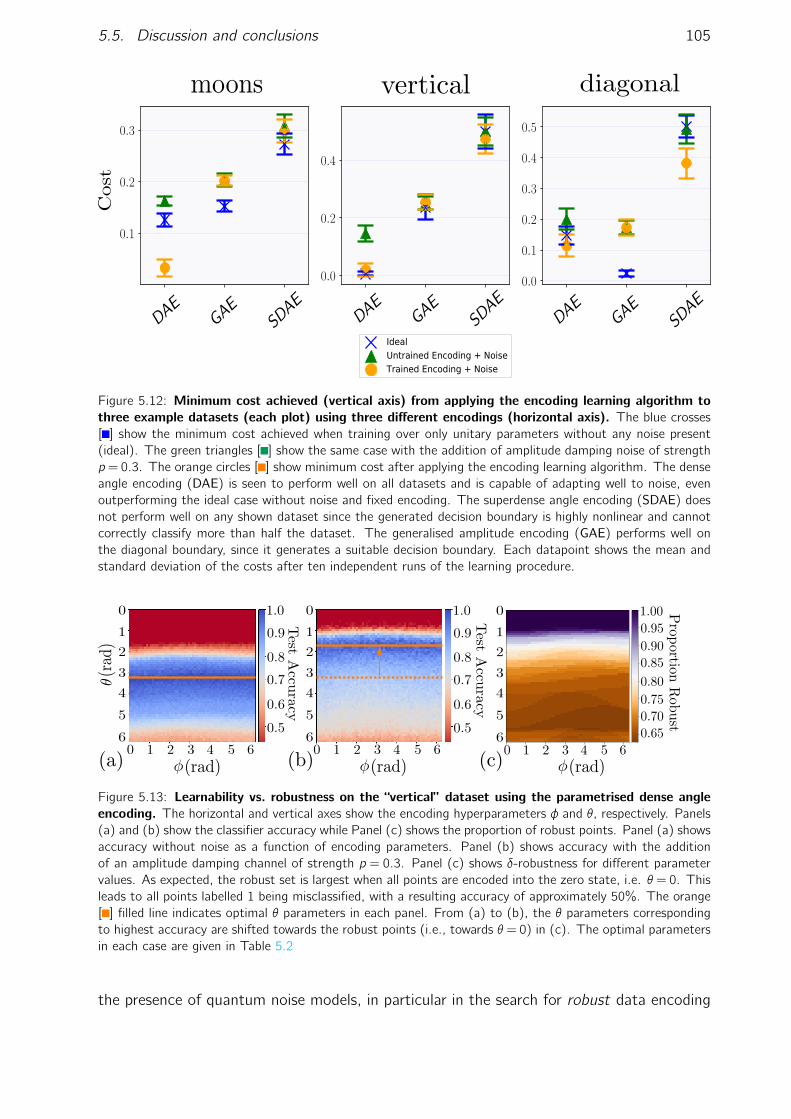
5.5. Discussion and conclusions 105
Ideal
Untrained Encoding + Noise
Trained Encoding + Noise
Figure 5.12: Minimum cost achieved (vertical axis) from applying the encoding learning algorithm tothree example datasets (each plot) using three different encodings (horizontal axis). The blue crosses[ ] show the minimum cost achieved when training over only unitary parameters without any noise present(ideal). The green triangles [ ] show the same case with the addition of amplitude damping noise of strengthp= 0.3. The orange circles [ ] show minimum cost after applying the encoding learning algorithm. The denseangle encoding (DAE) is seen to perform well on all datasets and is capable of adapting well to noise, evenoutperforming the ideal case without noise and fixed encoding. The superdense angle encoding (SDAE) doesnot perform well on any shown dataset since the generated decision boundary is highly nonlinear and cannotcorrectly classify more than half the dataset. The generalised amplitude encoding (GAE) performs well onthe diagonal boundary, since it generates a suitable decision boundary. Each datapoint shows the mean andstandard deviation of the costs after ten independent runs of the learning procedure.
0 1 2 3 4 5 6
0
1
2
3
4
5
6
[ , ] [ , ]
0.65
0.70
0.75
0.80
0.85
0.90
0.95
1.00
ib
Figure 5.13: Learnability vs. robustness on the “vertical” dataset using the parametrised dense angleencoding. The horizontal and vertical axes show the encoding hyperparameters φ and θ, respectively. Panels(a) and (b) show the classifier accuracy while Panel (c) shows the proportion of robust points. Panel (a) showsaccuracy without noise as a function of encoding parameters. Panel (b) shows accuracy with the additionof an amplitude damping channel of strength p = 0.3. Panel (c) shows δ-robustness for different parametervalues. As expected, the robust set is largest when all points are encoded into the zero state, i.e. θ = 0. Thisleads to all points labelled 1 being misclassified, with a resulting accuracy of approximately 50%. The orange[ ] filled line indicates optimal θ parameters in each panel. From (a) to (b), the θ parameters correspondingto highest accuracy are shifted towards the robust points (i.e., towards θ = 0) in (c). The optimal parametersin each case are given in Table 5.2
the presence of quantum noise models, in particular in the search for robust data encoding
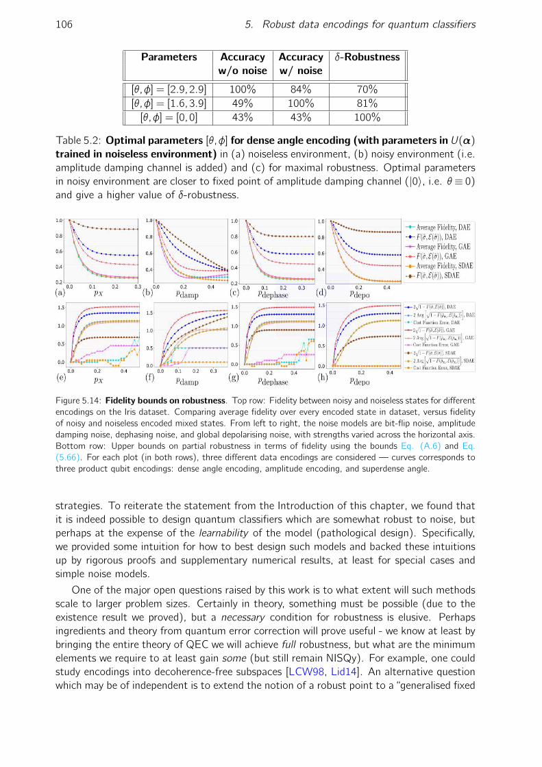
106 5. Robust data encodings for quantum classifiers
Parameters Accuracy Accuracy δ-Robustnessw/o noise w/ noise
[θ,φ] = [2.9,2.9] 100% 84% 70%
[θ,φ] = [1.6,3.9] 49% 100% 81%
[θ,φ] = [0,0] 43% 43% 100%
Table 5.2: Optimal parameters [θ,φ] for dense angle encoding (with parameters in U(α)
trained in noiseless environment) in (a) noiseless environment, (b) noisy environment (i.e.amplitude damping channel is added) and (c) for maximal robustness. Optimal parametersin noisy environment are closer to fixed point of amplitude damping channel (|0〉, i.e. θ≡ 0)and give a higher value of δ-robustness.
Figure 5.14: Fidelity bounds on robustness. Top row: Fidelity between noisy and noiseless states for differentencodings on the Iris dataset. Comparing average fidelity over every encoded state in dataset, versus fidelityof noisy and noiseless encoded mixed states. From left to right, the noise models are bit-flip noise, amplitudedamping noise, dephasing noise, and global depolarising noise, with strengths varied across the horizontal axis.Bottom row: Upper bounds on partial robustness in terms of fidelity using the bounds Eq. (A.6) and Eq.(5.66). For each plot (in both rows), three different data encodings are considered — curves corresponds tothree product qubit encodings: dense angle encoding, amplitude encoding, and superdense angle.
strategies. To reiterate the statement from the Introduction of this chapter, we found thatit is indeed possible to design quantum classifiers which are somewhat robust to noise, butperhaps at the expense of the learnability of the model (pathological design). Specifically,we provided some intuition for how to best design such models and backed these intuitionsup by rigorous proofs and supplementary numerical results, at least for special cases andsimple noise models.
One of the major open questions raised by this work is to what extent will such methodsscale to larger problem sizes. Certainly in theory, something must be possible (due to theexistence result we proved), but a necessary condition for robustness is elusive. Perhapsingredients and theory from quantum error correction will prove useful - we know at least bybringing the entire theory of QEC we will achieve full robustness, but what are the minimumelements we require to at least gain some (but still remain NISQy). For example, one couldstudy encodings into decoherence-free subspaces [LCW98, Lid14]. An alternative questionwhich may be of independent is to extend the notion of a robust point to a “generalised fixed

5.5. Discussion and conclusions 107
point” of a channel, i.e. points which satisfy f (E(ρ)) = f (ρ) for some function f . (Whenf = y , the “generalised fixed point” is a robust point, but other arbitrary functions f couldbe considered.) In a more empirical research direction, perhaps using machine learning itselfto find robust encodings will be fruitful (as initiated with our QELA), or even just extendingthis work to larger datasets (e.g., the MNIST dataset [LBBH98]) and more sophisticatedmodel design (for example by incorporating “data re-uploading” [PSCLGFL20] - more aboutthis in Sec. 5.5.1).
In conclusion, this chapter evidences that application-specific robustness (for (varia-tional) quantum algorithms in general) is a promising and interesting direction of study.
5.5.1 Subsequent work
In order to properly insert our work from this chapter in its proper context in the literature,we believe it is important to not only discuss the work which came before, but also subse-quent work which came after. To this end, we briefly summarise some we find interesting,which may be merged with our work, and the other future research directions given the pre-vious section. First, and perhaps most importantly, [SSM21, GVT20] highlighted explicitlythe effect of the data encoding on the function families representable by quantum modelssuch as ours. Interestingly, the authors found that by using data-reuploading [PSCLGFL20]the model can be expressed as a Fourier series, whose frequencies and coefficients aregiven by the data uploading and parameterised unitaries respectively. This reinforces ourfindings regards the importance of clever data encodings for the purpose of robustness.Secondly, on the theoretical side, there has been a flurry of work studying such quantummodels regarding their generalisation ability. For example, metrics such as the effectivedimension [ASZ+21], the capacity [WM20], the pseudo-dimension [CD20] among oth-ers [BKL+21b, BKL+21c, BKL+21d, GvVD21, HBM+21] have proven useful in derivingbounds on the generalisation of such models, which are key in further understanding them.It would be particularly interesting to study the relationship between these concepts, andthe ideas in this chapter. For example, one may examine the effect on these generalisationbounds when one is restricted to a specific set of robust points for a given noise channel.
Secondly, there have also been several works following ours considering the link betweennoise and defences against adversarial attacks in a quantum setting. For example, [LW20]demonstrated how, in high dimensions, it is easy for an adversary to perturb a quantumstate such that it is misclassified. The work of [DHL+21] showed how the simple quantumnoise models studied in this chapter could lead to ‘natural’ versions of differential privacy.Finally, [GFY21] and [WLL+21] derive robustness bounds to complement our own based onthe distance measures discussed in Sec. 2.1.7.2. The latter also demonstrated a link betweenrobust classification and quantum hypothesis testing, revealing an interesting avenue withwhich to explore in future work.
Finally, one may consider the more general influence of noise on NISQ algorithms. As wetouched on in Sec. 4.1.3, noise may exacerbate the effect of barren plateaus ([WFC+21]),or enable the efficient classical simulation of such quantum models [FGP20]. Alternatively,quantum error mitigation [ECBY21] may also be considered as a complementary techniqueto robustness, which is a rapidly expanding area of study.


6
Generative modelling with quantumcircuit Born machines
6.1 Introduction
“What an AI cannot create, it cannot understand.”– Ian Goodfellow, paraphrased from Richard Feynman
In the previous chapter, we discussed an application of VQAs in machine learning using aquantum classifier. These models are relatively simple, in the sense that supervised learning(classically) is quite well explored both from a theoretical and from an implementationpoint of view. In contrast, unsupervised learning is significantly more challenging and thischapter is dedicated to the generative modelling unsupervised learning problem (discussedin Sec. 3.3.2), and the model for this task which we introduced in Sec. 4.1.4, called thequantum circuit Born machine (QCBM).
We begin by recalling most ‘vanilla’ form of the quantum circuit Born machine (QCBM)from Sec. 4.1.4. Specifically, this involved the preparation of a parametrised state, |ψ(θ)〉,via a quantum circuit, U(θ), acting on a fixed initial state |0〉⊗n. The generative modelwhich this produces is the distribution given by measuring all qubits in the computationalbasis:
pθ(x) := |〈x |U(θ)|0〉⊗n|2 (6.1)
As a reminder, the task of generative modelling is to learn a representation of some datadistribution, q(y), given a set of samples, y jMj=1 from q. In practice, this means fittingthe parameters of the generative model (the QCBM), θ, such that pθ(x)≈ q(x) ∀x . Thisis usually achieved via the minimisation of some ‘distance’, d, between pθ and q (so theproblem is ‘solved’ when d(pθ,q)→ 0, recall the requirement of faithfulness from Sec. 4.1.1).
Given this problem statement, the goal of this chapter is threefold. We investigate theQCBM in some detail and in doing so we provide the following contributions:
• A discussion of quantum advantage using the QCBM. In simple terms, the ability tosolve a generative modelling problem better than any classical model could. Slightlymore precisely, given a distribution, q, output pθ which is ‘closer’ - with respect tosome distance measure - than any classical generative model could achieve.
• Improved differentiable training methods for the QCBM. Informally, better methodsto ‘fit’ the model parameters θ so that pθ is closer to q.
109

110 6. Generative modelling with quantum circuit Born machines
• A numerical comparison study of the QCBM versus a comparable classical model(specifically the restricted Boltzmann machine (RBM) discussed in Sec. 3.3.2) in aclose-to-real-world use case in finance.
Let us begin our adventure with a discussion of quantum advantage in generative mod-elling, using a QCBM.
6.2 Quantum advantage in generative modelling
Before diving into quantum advantage may arise in generative modelling, let us first motivatewhy such a thing might be feasible in the first place.
The reason is because the a core ingredient in generative models is sampling. It turns out,due to the probabilistic nature of quantum mechanics, sampling from a quantum distributionis a very straightforward thing to do (as we discussed in Sec. 4.1.4). This observationprompted the development of quantum computational supremacy (QCS)1, which refersto a specific task: the generation of samples from a quantum state, which could not begenerated by any classical algorithm, in a reasonable time. The reason for defining such anabstract problem, is primarily to illustrate the power of NISQ computers. NISQ computerscannot perform complex algorithms due to noise limitations (see Sec. 2.1.5), but what theycan do is prepare a quantum state via a short-depth quantum circuit, U, and measure allqubits in the computational basis. This then defines a natural sampling problem. Thequestion to demonstrate QCS is then twofold:
• Ensure U is simple enough to implement physically on NISQ devices.
• Prove rigorously that the sampling problem cannot be solved classically.
To achieve the former, a number of quantum circuit families have been proposed, includinginstantaneous quantum polynomial time (IQP) circuits, BosonSampling, and random circuitsampling (RCS). All of these proposals define sub-universal complexity classes in that theycannot implement an arbitrary quantum computation in BQP (see Sec. 2.1.2), but yet theyare still complex enough to be difficult to simulate classically (or so we believe). Excluding asimple preparation and measurement operation, IQP contains only gates which are diagonalin the computational (Pauli-Z) basis, BosonSampling involves interacting photonic modesin an interferometer without feedforward, and RCS involves implementing random layers ofhardware native locally connected gates.
The next ingredient is to prove such sampling tasks cannot be achieved classically2. Themost common route to do so, is to assume it can be simulated classically, and then derivean unlikely consequence in complexity theory, i.e. the collapse of the polynomial hierarchy([Sto76])3. Such a collapse occurring is a generalisation of P being equal to NP, which iswidely believed to be not the case.
1Also called quantum superiority, or more commonly quantum advantage to avoid any controversies.2By ‘achieved’ here, we mean cannot by simulated in polynomial time - if classical simulators are allowed
to take exponential time then we know then would be able to simulate quantum computers by just keepingtrack of the exponentially large wavefunction.
3An introduction to (quantum) complexity theory is not necessary for reading this theses, and so for acomprehensive overview of this topic see [NC10] as well as the complexity zoo for a list of complexity classes.

6.2. Quantum advantage in generative modelling 111
6.2.1 The Ising Born machine
In the work of a previous dissertation [Coy18], we introduced a specification of a QCBMbased on a generalisation of IQP circuits which we dubbed the quantum circuit Ising Bornmachine (QCIBM). This model was a generalisation because we added the possibility ofmeasurement in alternative bases (standard IQP circuits only measures in the Hadamardbasis). Specifically, the circuits considered for the QCIBM had the following structure (wereintroduce it here from [Coy18] since we use this same model in our numerical results laterin this thesis):
|0〉 H
Uz(α)
U1f (Γ1,∆1,Σ1) x1
|0〉 H U2f (Γ2,∆2,Σ2) x2
· · · · · · · · ·
|0〉 H Unf (Γn,∆n,Σn) xn
(6.2)
where: xi ∈ 0,1; the unitaries are defined by Eq. (6.3) and Eq. (6.4); Sj indicates thesubset of qubits on which each operator, j , is applied; and α := αj are the trainableparameters.
Uz(α) := ∏j
Uz(αj ,Sj
)= ∏
j
exp
iαj⊗k∈Sj
Zk
(6.3)
Uf (Γ,∆,Σ) := exp
(in
∑k=1
ΓkXk + ∆kYk + ΣkZk
)(6.4)
The model was dubbed ‘Ising’ since restricting to the case |Sj | 6 2 (since only single andtwo-qubit gates are required for universal quantum computation) the term in the exponentialof Eq. (6.3) becomes exactly the Ising Hamiltonian discussed in Eq. (4.5).
Furthermore, we also showed in [Coy18] how the shallowest depth (p= 1) version of theQAOA algorithm (see Eq. (4.10) in Sec. 4.1.2) could also be recovered by a specific settingof the final measurement angles in Eq. (6.4).
By inheriting the ‘hardness’ results of standalone IQP and p = 1 QAOA circuits [BJS11,FM17, FH16], we could show that the QCIBM remained in the same complexity class asthe the standalone versions during training of the generative model, and then also samplingfrom a QCIBM could not be simulated classically (up to multiplicative error).
However, while hardness-of-simulating the generative model is at least an important stepon the road to true quantum advantage4, it is not the end of the story. One would also liketo make a case for the hardness of learning, i.e. that the QCIBM (or indeed any quantumgenerative model) could learn a distribution which could not be learned classically. Such a‘quantum learning advantage’ (especially in a near-term NISQy regime) would be concreteproof of the usefulness of quantum machine learning.
4It surely is at least a necessary condition; if it was possible to classically simulate the generative quantummodel at each point during training - one could just use the classical simulation instead of having to actuallybuild a quantum computer (which would be significantly more expensive, from a practical sense).

112 6. Generative modelling with quantum circuit Born machines
6.2.2 The supremacy of quantum learning
The contribution of this section is to formalise this question, using concepts from learningtheory, and provide an initial attempt at showing such an advantage, by focusing on the‘hard-to-simulate’ quantum supremacy circuits discussed above. We call this quantum learn-ing supremacy (QLS) to parallel the corresponding QCS which deals exclusively with theunderlying sampling problem. Informally a generative quantum machine learning algorithmis said to have demonstrated QLS, if it is possible for it to efficiently learn a representationof a distribution for which there does not exist a classical learning algorithm achieving thesame end. More specifically, the quantum device has the ability to produce samples accord-ing to a distribution that is close in total variation distance (Eq. (2.48))5 to some targetdistribution, using a polynomial number of samples from the target.
To begin, we must understand the inputs and outputs to learning algorithm, for whichwe have a certain amount of freedom. The inputs are samples, either classical vectors, orquantum states encoding a superposition of such bitstring states, i.e. qsamples [SP18] (aspecial case of the amplitude encoding from Definition 22):
Definition 38 (Qsample).Given a discrete probability distribution, [p(x1),p(x2), . . . ,p(x2n)]T , x i ∈ 0,1n, aqsample encoding of this distribution maps p(x)→ Eqsamp given by:
Eqsamp : p(x i)i → |p(x)〉 :=2n
∑i=1
√p(x i)|x i〉 (6.5)
The state in Eq. (6.5) is clearly a generalisation of the classical distribution, since wecan measure all qubits in the computational basis, and we will recover the sample x i withthe correct probability,
√p(x i)
2= p(x i). Giving the learning algorithm to classical samples,
x i or a quantum superposition over all possible samples (i.e. a qsample, Eq. (6.5)) can leadto advantages in supervised learning theory [SG04], so it is not unreasonable to expect ananalogue is possible for generative modelling.
While the sample complexity of quantum versus classical learning has been studied in thesupervised learning sense (see the discussions in Sec. 3.6 and Sec. 4.3), the same cannotbe said about unsupervised learning. Fortunately, we do have a framework in the classicalsetting for studying distribution learning problems, so-called distribution learning theory,introduced by [KMR+94]. Here we bring this forward to the quantum setting.
Unlike the supervised setting, there are more than one type of ‘learner’ (or more than twoif one also counts the quantum generalisation). We can define distribution learners whichmuch learn solely from samples from the distribution (learning with Generators), and thosewhich can learn from the probabilities themselves (learning with Evaluators). For simplicity,we assume the distributions classes in question (as in [KMR+94]), are discrete over binaryvectors of length n, denoted Dn. Let us now define Generators and Evaluators:
5The reason for this choice will become apparent shortly.
6.2. Quantum advantage in generative modelling 113
Definition 39 (Generator [KMR+94]).A class of distributions, Dn, has efficient Generators, GEND, if for every distributionD ∈ Dn, GEND produces samples in 0,1n according to the exact distribution D,using polynomial resources. The generator may take a string of uniformly randombits, of size polynomial in n, r(n), as input.
Notice this definition allows, for example, for the Generator to be either a classicalcircuit, or a quantum circuit, with polynomially many gates. Further, in the definition of aclassical Generator [KMR+94] a string of uniformly random bits is taken as input, and thentransformed into the randomness of D. However, a quantum Generator would be able toproduce its own randomness and so no such input is necessary. In this case the algorithmcould ignore the input string r(n).
Definition 40 (Evaluator [KMR+94]).A class of distributions, Dn has efficient Evaluators, EVALD, if for every distributionD ∈ Dn, EVALD produces the weight of an input x in 0,1n under the exact distri-bution D, i.e. the probability of x according to D. The Evaluator is efficient if it usespolynomial resources.
The distinction between EVAL and GEN is important and interesting since the outputprobabilities of IQP circuits are #P-Hard to compute and also hard to sample from byclassical means, as discussed above [BJS11], yet the distributions they produce can besampled from efficiently by a quantum computer. This draws parallels to examples in[KMR+94] where certain classes of distributions are shown not to be learnable efficientlywith an Evaluator, but they are learnable with a Generator.
For our purposes, the following definitions of learnable will be used. In contrast to[KMR+94], which was concerned with defining a ‘good’ generator to be one which achievescloseness relative to the KL divergence (Eq. (2.49)), we wish to expand this to general costfunctions, d . The reason for this will become apparent later on, when dive into quantumsampling hardness results (high typically strive for closeness in TV) in more detail, and whenwe introduce our new training methods for the QCIBM .
Definition 41 ((d,ε)-Generator).For a cost function, d, let D ∈ Dn. Let GEND′ be a Generator for a distribution D′.We say GEN is a (d,ε)-Generator for D if d(D,D′)6 ε.
A similar notion of an ε-good Evaluator could be defined.

114 6. Generative modelling with quantum circuit Born machines
Definition 42 ((d,ε,C)-Learnable).For a metric d, ε > 0, and complexity class Ca, a class of distributions Dn is called(d,ε,C)-learnable (with a Generator) if there exists an algorithm A ∈ C, called alearning algorithm for Dn, which given 0< δ < 1 as input, and given access to GENDfor any distribution D ∈ Dn, outputs GEND′, a (d,ε)-Generator for D, with highprobability:
Pr[d(D,D′
)6 ε]> 1− δ (6.6)
A should run in time poly(1/ε,1/δ,n).
aThe introduction of a complexity class here should not be considered rigorous, but is used to allowthe algorithm to be either quantum or classical in nature.
Finally, we define what it would mean for a quantum algorithm to be superior to any classicalalgorithm for the problem of distribution learning, before moving onto our initial attempt toachieve such a thing:
Definition 43 (Quantum learning supremacy (QLS)).An algorithm A ∈ BQP is said to have demonstrated the supremacy of quantumlearning over classical learning if there exists a class of distributions Dn for whichthere exists d,ε such that Dn is (d,ε,BQP)-Learnable, but Dn is not (d,ε,BPP)-Learnable.
6.2.3 Quantum learning supremacy via quantum computational supremacy
Let us now move onto an initial attempt to achieve QLS. Since this question of distributionlearning advantage is motivated by the classical hardness of sampling from the distributionsgenerated by a quantum circuit, a natural distribution class, Dn to learn would be exactlythese ‘quantum supremacy distributions’. We focus on IQP circuits as a concrete example,although a similar logic could in principle be applied to alternative QCS candidates suchas BosonSampling or RCS. For QCS, there are a number of further subtleties which mustbe address including: worst versus average case hardness of classical simulation, and thenotions of the ‘error’ of such simulations, which relate to the probability metrics introduced inSec. 2.1.7.1. For our present discussion, the latter is more relevant, although for discussionsof the former and a comparison between the different QCS proposals, see [HM17, BFNV19].
The most common error models used in proofs of QCS are multiplicative and additive(or total variation) error:
Definition 44 (Multiplicative error).A circuit family is weakly simulatable within multiplicative (relative) error, if thereexists a classical probabilistic algorithm, Q, which produces samples, x , according tothe distribution, q(x), in time which is polynomial in the input size, which differs fromthe ideal quantum distribution, p(x), by a multiplicative constant, c > 1:
1
cp(x)6 q(x)6 cp(x) ∀x (6.7)

6.2. Quantum advantage in generative modelling 115
It would be desirable to have a quantum sampler which could achieve the bound of Eq.(6.7), but this is not believed to be experimentally achievable, i.e. it is not believed that aphysical quantum device could achieve such a multiplicative error bound on its probabilities,relative to its ideal functionality (i.e. replacing q in Eq. (6.7) by the output distribution ofa noisy quantum device). That is why much effort has been put into trying to find systemsfor which QCS could be provably demonstrated according to the total variation distanceerror condition, Eq. (6.8), which is easier to achieve on near term quantum devices.
Definition 45 (Total variation (TV) error).A circuit family is weakly simulable within variation distance error, ε, if there existsa classical probabilistic algorithm, Q, which produces samples, x , according to thedistribution, q(x), in polynomial time, such that it differs from the ideal quantumdistribution, p(x) in total variation distance, ε:
TV(p,q) :=1
2 ∑x
|p(x)−q(x)|6 ε (6.8)
It has been proven that weakly simulating IQP circuits to a fixed TV error is classicallyhard. Specifically, if a classical algorithm could sample from a distribution, q, for whichTV(p,q)6 1/384, where p is the output distribution from an IQP circuit, then the polyno-mial hierarchy would collapse to the third level (see [BMS16] for a formal statement of therelevant theorem), assuming the hardness of computing the Ising partition function.
Now, where does QLS fit into this? Well, let us revisit the relationship between thesedefinitions, and those for distribution learning in Sec. 6.2.2. Firstly, note that there is adirect and obvious connection to the ‘strength’ of classical simulators of quantum circuits.
The two primary types of classical simulation are strong and weak6 simulators:
Definition 46 (Strong and weak classical simulation [BJS11, FM17]).A uniformly generated quantum circuit, C, from a family of circuits, with input size n,is weakly simulatable if, given a classical description of the circuit, a classical algorithmcan produce samples, x , from the output distribution, p(x), in poly(n) time.On the other hand, a strong simulator of the family would be able to compute theoutput probabilities, p(x), and also all the marginal distributions over any arbitrarysubset of the outputs. Both of these apply with some notion of error, ε.
As mentioned in [BJS11], strong simulation is a harder task than weak simulation, and itis this weak simulatability which we want to rule out as being classically hard, since it bettercaptures the process of sampling. The suitable notion of error, ε, for strong simulationwould be the precision to which the probabilities can be computed. Recalling the definitionsin Sec. 6.2.2, it is clear that an Evaluator for a quantum circuit would be a strong simulatorof it, and a Generator would be a weak simulator.
Next, let us take the learning metric in Definition 43, to be the total variation distance,d = TV, and let Dn be the family of IQP distributions. Imagine, we were able to concocta learning algorithm, A (for example the QCIBM), to output a generator for a distribu-tion, DQCIBM, (GENDQCIBM
) given poly many samples (classical or quantum) from an IQPdistribution, DIQP. Furthermore, assume we have TV(DQCIBM,DIQP)6 γ.
6We already used this terminology in Definition 44 and Definition 45.

116 6. Generative modelling with quantum circuit Born machines
Now, assuming DQCIBM distributions are classically easy to emulate7 within a fixedTV error, δ, meaning there exists a classical probabilistic algorithm, C, could output adistribution, DC such that:
TV(DC,DQCIBM)6 δ (6.9)
Then, by a simple triangle inequality argument, we have:
TV(DIQP,DC) =1
2 ∑x
|DIQP(x)−DC(x)| (6.10)
=1
2 ∑x
|DIQP(x)−DQCIBM(x) +DQCIBM(x)−DC(x)| (6.11)
61
2 ∑x
|DIQP(x)−DQCIBM(x)|+1
2 ∑x
|DQCIBM(x)−DC(x)| (6.12)
6 δ+γ =: ε=1
384(6.13)
Therefore, if we are able to make δ+γ smaller than 1/384, we arrive at a contradictionto the result of [BMS16], and as such, DQCIBM must also be difficult to simulate within asmall fixed TV distance. As a result, something classically infeasible has been achieved8.
This above discussion covers the ‘classical hardness’ of the learning task, but we haveyet to discuss the feasibility of the learning problem itself, i.e. outputting a generatordistribution achieving γ closeness in TV to an IQP distribution.
Unfortunately, it is here the argument appears to fail. A key ingredient in proofs of thehardness of classically simulating quantum supremacy distributions is the property of anti-concentration, which formally means that given a random instance from a ‘hard’ circuitfamily, for example an instance of an IQP circuit, then it does not become too unlikely thatthe probability of any fixed outcome, x , by measuring the state U|0〉⊗n, is much smaller thanit would be if x was drawn from the uniform distribution. In other words, anti-concentrateddistributions are ‘exponentially flat’:
∃α,γ > 0,s.t.∀x ∈ 0,1n, PrU∼µ
(pU(x) := |〈x |U|0〉n|2 >
α
2n
)> γ, (6.14)
where the unitary is drawn according to a measure µ on the unitary group.Now comes the rub; the work of [HKEG19] proved that verifying such anti-concentrating
distributions, for example IQP9 would require exponentially many samples from the distri-bution to be verified. Verification in this sense means building a ‘testing’ algorithm whichcan distinguish whether the distribution to be verified is far or close to the ideal distributionin TV.
As a consequence of this no-go result, one can conjecture that also building an efficientGenerator for an anti-concentrating distribution is also not feasible. This is because onecould imagine a verification algorithm to be a subroutine in any learning algorithm attemptingto demonstrate QLS. The key property of QCS circuit families being hard to simulate, is also
7In other words, proof by contradiction.8A very related idea was proposed by [RGS+18], where the authors studied the learnability of classical hard
distributions using (classical) variational autoencoders.9It was also proven for BosonSampling and RCS. For IQP this anti-concentration behaviour has been
explicitly proven, for BosonSampling on the other hand it is only a (believeable) conjecture.

6.3. Training a quantum circuit Born machine 117
what makes them hard to learn. However, the above discussion assumed efficient classicalsample access to the QCS distribution - it may be possible to bypass the classical no-gotheorem given qsample access.
To conclude, we note that at the time of writing the question of a near-term quantumadvantage in generative modelling is still an open question. However, since the completionof the works in this chapter, some interesting progress was made towards this goal. Wereturn to this discussion in the conclusion.
6.3 Training a quantum circuit Born machine
Let us now introduce our second contribution in the subject of quantum generative mod-elling. As mentioned in Sec. 6.1 this will be the introduction of new gradient based trainingmethods for the quantum circuit Born machine. We will use primarily the QCIBM as aspecific instance, but remark that everything presented in this section applies generally toQCBMs. We already introduced much of the relevant details for this section in Sec. 2.1.7.1which described various measures on the space of probability distributions.
Recall in Sec. 2.1.7.1 we introduced two families of distribution measures, specificallyf -divergences (Eq. (10)), and integral probability metrics (IPMs) (Eq. (11)). In order totrain generative models, these probability measures will serve as our ‘cost functions’, C, asin Sec. 4.1.1. Since quantum circuit Born machines are just a special case of variationalalgorithms applied to generative modelling, we similarly wish for the cost functions we useto have the same well defined properties as with any VQA (discussed in Sec. 4.1.1), namelyfaithfulness, efficient computability and operational meaning. We go into significant detailwith these properties in this sections since they turn out to be extremely important fortraining generative models.
Let us begin by discussing f -divergences, any why they may not satisfy the ‘efficientcomputability’ criterion. Let us take the KL divergence as a special case. Rewriting Eq.(2.49) in terms of the model distribution (specifically the QCIBM output distribution), pθ,and let us use the notation, π to denote the ‘data’ distribution we are trying to fit:
CKL(θ) := KL(π,pθ) := ∑x
π(x) logπ(x)−∑x
π(x) logpθ(x) (6.15)
Since the first term (the entropy of π) is constant with respect to pθ, when solvingthe optimisation, argminθCKL(θ), it can be ignored. Therefore, we now solve insteadargmaxθXE(π,pθ). However, recall in Sec. 6.2, we discussed how computing the outcomeprobabilities of quantum circuits was #P-hard, hence we may require exponential resourcesto get a good estimate of pθ(x) for all x ∈ 0,1n. Since the expression in Eq. (6.15) can-not be written as a sampling expression over pθ10, we do not expect to be able to efficientlycompute the term XE(π,pθ), and hence we cannot compute KL(π,pθ). This was realisedspecifically for the case of QCBMs by [LW18a], where the corresponding gradients of the
10By this we mean that the KL divergence cannot be written in terms of quantities like Ex∼pθ
(·), which can
be estimated by simply drawing samples from pθ. Terms of this form can usually be estimated more efficientlysince we only need to sample the high-probability values, x , to get a good estimate of the expectation value- we do not necessarily need to know the probability at every x (of which there are exponentially many)

118 6. Generative modelling with quantum circuit Born machines
L parameters in a QCBM were computed and found to be11:
∂KL∂θk
=−∑x
π(x)pθ−k−pθ+
k
pθ(6.16)
where we use the notation θ±k := (θ1,θ2, . . . ,θk ± π/2, . . . ,θL) to denote the parameter shiftrule in Eq. (4.13). Hence, if we cannot compute the probabilities pθ(x) efficiently, we willnot be able to compute neither f -divergences, nor their gradients. A solution to this wasrealised by [LW18a] (which we alluded to in Sec. 2.1.7.1), which was to instead use theMMD Eq. (2.54) to efficiently train QCBMs in a differentiable manner. Since the MMDcan be written exclusively as expectation values over the data distribution and the QCBMdistribution it can be evaluated efficiently (specifically with the quadratic sample complexityof Eq. (2.56)). The same can be said for its gradients, which were computed by [LW18a]to be:∂CMMD(pθ,π)
∂θk= 2Ea∼p−θkx∼pθ
(κ(a,x))− 2Eb∼p+
θkx∼pθ
(κ(b,x))− 2Ea∼p−θky∼π
(κ(a,y)) + 2Eb∼p+
θky∼π
(κ(b,y)) (6.17)
where we define CMMD := MMDκ from Eq. (2.54).Both of the cost functions we have discussed so far are ‘faithful’, meaning in this case
that C(pθ,π) = 0 ⇐⇒ pθ = π (by definition, since they are a divergence, and a metricbetween probability distributions respectively12). We have established how the MMD isan efficient method to train QCBMs (and generative models generally), whereas the KLdivergence may not be. The final quality we have not touched upon is the operationalmeaning of these cost functions, which we take in this sense to be how ‘powerful’ they areas training mechanisms.
By this, we mean their performance and properties relative to TV13. Firstly, it is clearthat the KL divergence is stronger than TV since the upper bound it provides via Pinsker’sinequality Eq. (2.50). Hence, if we were able to efficiently train a QCBM with the KLdivergence to a particular value, we can directly upper bound the TV from this value -closeness in KL implies closeness in TV.
The same cannot be said unfortunately about the MMD. Specifically, the MMD providesonly a lower bound on TV from [SFG+09]:
TV(pθ,π)>
√MMD(pθ,π)√
k(6.18)
if we have that k := supx∈X n κ(x ,x) <∞. For example, taking the Gaussian kernel Eq.(3.23) (or even the quantum kernel Eq. (4.30)), we have:
κG(x ,x) = e−12 |x−x |
2
= 1 (6.19)11An important point to note here, we have a slightly different functional form for the gradients than those
presented in [LW18a]. This is because we will be using these gradients to train the QCIBM in Eq. (6.2), andthe gates in this circuit are of the form eiθΣ, rather than e−i(θ/2)Σ. These are essentially equivalent at anyrate, and only introduce an alternative factor in front of the gradient term to change its magnitude. We willuse this formulation of the gradient for all the cost functions described here.
12A subtle point for the diligent reader: it may be expected that the faithfulness of the MMD must havesomething to do with the kernel function and feature map - indeed this is true, the MMD is only faithful ifthe corresponding kernel is ‘universal’. We return to a discussion of kernel universality later in this Thesis.
13We take this viewpoint specifically in light of our discussion of QLS in Sec. 6.2, where total variationdistance is the relevant measure.

6.3. Training a quantum circuit Born machine 119
hence k = 1 and the lower bound is immediate. With this in mind (we will circle back tothis operational meaning afterwards), let us move onto the new cost functions we proposefor training a QCBM. These are the Stein discrepancy, and the Sinkhorn divergence.
6.3.1 Training with the Stein discrepancy
Firstly, let’s look at the Stein discrepancy (SD). The SD has become popular for goodness-of-fit tests [LLJ16], i.e. testing whether samples come from a particular distribution ornot14. This discrepancy is based on Stein’s method [Ste72], which is a way to bounddistance metrics between probabilities including, for example, IPMs.
The original formulation of the discrepancy was done in the the continuous case. How-ever, in the case of a QCBM, we require a discrete version of the discrepancy (since theoutput are samples, x ∈ 0,1n).
To set the scene, let us begin with the continuous version. A key ingredient is Stein’sidentity (in the case where the sample space is one-dimensional, x ∈ X ⊆ R) given by:
Eπ [Aπφ(x)] = Eπ [sπ(x)φ(x) +∇xφ(x)] = 0 (6.20)
where sπ(x) =∇x log(π(x)) is the Stein score function of the distribution π, ∇x f (x) is thegradient of a function, f and Aπ is a so-called Stein operator of π. The functions, φ, whichobey Eq. (6.20), are said to be in the Stein class15 of the distribution π. From Stein’sidentity, one can define a discrepancy between the two distributions, pθ,π, by the followingoptimisation problem, [YLRN18]:
dSD(pθ||π) := supφ∈F
(Epθ [Aπφ]−Epθ [Apθφ]
)2(6.21)
If pθ ≡ π, then dSD(pθ||π) = 0 by Eq. (6.20). Exactly as with the MMD, the power ofthe discrepancy in Eq. (6.21), will depend on the choice of the function space, F . Bychoosing it to be a RKHS, a kernelised form which is computable in closed form can beobtained. Also, this form of Eq. (6.21) is very reminiscent of that of the integral probabilitymetrics, Eq. (11) (and indeed the SD can be written in such a form where the functionfamily in the IPM is distribution-dependent).
From Eq. (6.21), the problem arises. Due to the gradient term, ∇x , in Eq. (6.20),the above expressions are only defined for smooth probability densities, pθ,π, which aresupported on continuous domains (e.g. R). Therefore, in order to make the SD compatiblewith training a QCBM, we must perform a discretisation procedure.
Fortunately, this has been addressed by [YLRN18], which adapted the kernelised SD tothe discrete domain. This was achieved by introducing a discrete gradient ‘shift’ operator.Just as above, let us assume we have n-dimensional sample vectors, x ∈ X n ⊆ Rn (whereX is a discrete set). First of all, we shall need some definitions [YLRN18]:
Definition 47 (Cyclic permutation).For a set X of finite cardinality, a cyclic permutation ¬ :X →X is a bijective functionsuch that for some ordering x [1],x [2], . . . ,x [|X |] of the elements in X , ¬ = ¬i : x [i ] 7→x [(i+1) mod |X |],∀i = 1,2, . . . , |X |
14In contrast, the MMD is typically used for kernel two-sample tests [GBR+07].15These functions, φ are essentially those which allow the identity to be proven via integration by parts, i.e.
those which are smooth and have appropriate boundary conditions.

120 6. Generative modelling with quantum circuit Born machines
Definition 48 (Partial difference operator and difference score function).Given a cyclic permutation ¬ on X , for any vector, x = [x1, . . . ,xn]T ∈ X n. For anyfunction f : X n→ R, denote the (partial) difference operator as:
∆xi f (x) := f (x)− f (¬ix) ∀i = 1, . . . ,d (6.22)
with ∆f (x) = (∆x1f (x), . . .∆xn f (x))T . Define the (difference) score function for apositive probability mass function, p(x)> 0 ∀x as:
sp(x) :=∆p(x)
p(x), (sp(x))i =
∆xip(x)
p(x)= 1−
p(¬ix)
p(x)(6.23)
Furthermore, [YLRN18] defines the inverse permutation by ¬=¬i : x [i ] 7→ x [(i−1) mod |X |],and the inverse shift operator by:
∆∗xi f (x) := f (x)− f (¬i x) ∀i = 1, . . . ,n (6.24)
For our purposes, this generalisation is actually not necessary. Since the sample space fora single qubit is binary, X = 0,1, the forward and reverse permutations are identical, so∆ = ∆∗. With this change to the gradient operator, [YLRN18] defines discrete versions ofthe Stein identity, and the kernelised Stein discrepancy which we can now state.
Theorem 15:For any functiona Φ :X n→Cm, and a probability mass function p on X n, the discreteStein identity is given by:
Ex∼p
[ApΦ(x)] = Ex∼p
[sp(x)Φ(x)T −∆Φ(x)
]= 0 (6.25)
where ∆Φ(x) is an n×m matrix: (∆Φ)i j = ∆xiΦj(x), i.e. shifting the i th element ofthe j th function value.
aWe have implicitly generalised the input space to be a vector space as in [YLRN18], but we havealso taken the possibility that the feature maps may be complex valued. This allows us the freedom touse quantum kernels for κ in place of purely classical ones. This is also possible due to the nature ofthe discretisation which results in all functions Φ : X n → Cm to be in the Stein class of the operatorAp. The proof of this is a simple adaptation of the corresponding proof in [YLRN18] for real valuedfunctions, and we omit it here.
6.3. Training a quantum circuit Born machine 121
We can then reproduce the following Theorem:
Theorem 16:The discrete kernelised SD between two distributions, p,q is given by:
CSD(p,q) := Ex ,y∼p [κq(x ,y)] (6.26)
where κq is the ‘Stein kernel’:
κq(x ,y) := sq(x)Tκ(x ,y)sq(y)− sq(x)T∆∗yκ(x ,y)
−∆∗xκ(x ,y)T sq(y) +Tr(∆∗x ,yκ(x ,y)) (6.27)
Let us pause briefly here to return to the discussion above regarding valid kernels. Asmentioned above, for the MMD to be faithful, its kernel must be characteristic or univer-sal [FGSS07, SGF+08]. The Gaussian kernel Eq. (3.23) is indeed one which is charac-teristic [FGSS07], and some effort has been made to find conditions under which a kernelis characteristic [SFL11]. If the sample space is discrete, it turns out the condition fordetermining universality is simpler. In this case we only require the Gram matrix for thekernel, Ki j = κ(x i ,y j) to be positive definite16 [SFG+09]. If the Gram matrix for a kernel ispositive definite we refer to the kernel itself as being strictly positive definite (confusingly).Just as with the MMD, it turns out this requirement of kernel-positive-definiteness is againexactly what makes the SD a valid discrepancy measure [YLRN18].
Next, we can compute the gradients of Eq. (6.26) as with those of the MMD (replacingp→ pθ,q→ π for the QCBM and data distributions):
∂CSD
∂θk= ∑x ,y
∂pθ(x)
∂θkκπ(x ,y)pθ(y) + ∑
x ,y
pθ(x)κπ(x ,y)∂pθ(y)
∂θk
= ∑x ,y
p−θk (x)κπ(x ,y)pθ(y)−∑x ,y
p+θk
(x)κπ(x ,y)pθ(y)
+ ∑x ,y
pθ(x)κπ(x ,y)p−θk (y)−∑x ,y
pθ(x)κπ(x ,y)p+θk
(y) (6.28)
∂CSD
∂θk= Ex∼p−θky∼pθ
[κπ(x ,y)]− Ex∼p+
θky∼pθ
[κπ(x ,y)] + Ex∼pθy∼p−θk
[κπ(x ,y)]− Ex∼pθy∼p+
θk
[κπ(x ,y)] (6.29)
Using again the parameter-shift rule Eq. (4.13) and that the Stein kernel, κπ, of Eq. (6.27)does not depend on the parameter, θk .
Clearly, the primary difference between the MMD and the SD is the form of the kernelwhich must be computed in each case. To compute the Stein kernel, we must evaluate thebase kernel κ for each pair of samples. Let us assume this costs time T (n) (a polynomialfunction of the number of qubits, n).
However, adding to the computational burden, we also must compute the following‘shifted’ versions of the kernel for each pair of samples, (x ,y), in both parameters:
∆xκ(x ,y) ∆yκ(x ,y) Tr [∆x ,yκ(x ,y)] (6.30)
16Recall, a matrix, K, is positive definite ⇐⇒ ∀x ∈ Rd/0, xTKx > 0.

122 6. Generative modelling with quantum circuit Born machines
which are required in Eq. (6.27). To compute one of these terms (for example, ∆xκ(x ,y)),we have:
∆xκ(x ,y) = [κ(x ,y), . . . ,κ(x ,y)]T − [κ(¬1x ,y), . . . ,κ(¬nx ,y)]T (6.31)
so we must evaluate κ(¬ix ,y) for i = 1, . . . ,n. Therefore, computing the shifted kerneloperator in a single parameter takes O(T (n)× (n+ 1)). The same holds for the kernelgradient with respect to the second argument, ∆yκ(x ,y). For ∆x ,yκ(x ,y), the process isslightly more involved because:
Tr [∆x ,yκ(x ,y)] = Tr (∆x [∆yκ(x ,y)]) = Tr (∆x [κ(x ,y)−κ(x ,¬y)]) (6.32)
= nκ(x ,y)−n
∑i=1
κ(x ,¬iy)−n
∑i=1
κ(¬ix ,y) +n
∑i=1
κ(¬ix ,¬iy) (6.33)
Each individual term in the respective sums requires the same complexity, i.e. O(T (n)) sothe term Tr [∆x ,yκ(x ,y)] overall requires O(T (n)× (3n+ 1)).
However, we have not yet discussed the computation of the score function, sπ. If weare given oracle access to the probabilities, π(y), then there is no issue and SD will becomputable. Unfortunately, in many practical applications this will not be the case. To dealwith this scenario, in Sec. 6.3.2.1 and Sec. 6.3.2.2, we give two methods to approximatethe score function, given samples from the dataset, π. Notice that even with this hurdle(difficulty in compute the score), the SD is still more suitable than the KL divergence totrain these models, since the latter requires computing the circuit probabilities, pθ(x), whichis in general intractable, and so could not be done for any dataset. In contrast, the Steindiscrepancy only requires the data probabilities, which may make it amenable for generativemodelling using some datasets.
6.3.2 Computing the Stein score function
Let us now discuss the final ingredient for the Stein discrepancy: the computability ofthe score function Eq. (6.23). For every sample, x ∼ pθ, that we receive from the Bornmachine we require the score function of that same outcome being outputted from thedata distribution, x ∼ π. This involves computing π(x), and also ∆xπ(x), i.e. π(¬ix),∀i ∈1, . . . ,n.
This section will discuss our approach to approximate the score function of the data,sπ, from samples, y i : y ∼ π(y), based on the methods of [LT18, SSZ18]. We call thesemethods the ‘Identity’, and ‘Spectral’ methods for convenience. Of course, the most obviousapproach to computing the score, usingM samples alone, would be to simply accumulate theempirical distribution which is observed by the samples, pθ(y) := 1
M ∑Sm=1 δ(y − y (m)) and
compute the score from this distribution. However, this immediately has a severe drawback.Since the score for a given outcome, sπ(xm), requires also computing the probabilities of allshifted samples, π(¬ixm) ∀i , if we have not seen any of the outcomes ¬ixm in the observeddata, we will not have values for these outcomes in the empirical distribution, and hencewe cannot compute the score. This would be a major issue as the number of qubits grows,since we will have exponentially many outcomes, many of which we will not see with poly(n)
samples.

6.3. Training a quantum circuit Born machine 123
6.3.2.1 Identity approximation of Stein score
As a first attempt, we adopt the method of [LT18]. This involves noticing that the scorefunction appears explicitly in Stein identity, and inverting Stein’s identity gives a procedureto approximate the score (hence we dub this approach the ‘Identity’ method).
Of course, we shall need to use the discrete version of Stein’s identity in our case, andre-derive the result of [LT18] but there are no major difficulties in doing so.
Let us define the ‘score matrix’, G, using M samples drawn from π:
Gπ :=
s1π(x1) s1
π(x2) . . . s1π(xM)
s2π(x1) s2
π(x2) . . . s2π(xM)
...... . . . ...
snπ(x1) snπ(x2) . . . snπ(xM)
Gπi,j := siπ(x j) =∆x jiπ(x j)
π(x j)(6.34)
Each column is the term which corresponds to the score function for the distribution, π,and that given sample.
Now, to compute an approximation of Gπ: Gπ ≈ Gπ we can invert the discrete versionof Stein’s Identity, Eq. (6.35) (as in the continuous case of [LT18]):
Ex∼π
[sπ(x)Φ(x)T −∆f(x)] = 0 (6.35)
where f is a complex vector valued ‘test’ function.Rearranging Eq. (6.35) in terms of the score, and following [LT18]:
Ex∼π
[sπφ(x)T ] = Ex∼π
[∆f(x)] =⇒ ∑x
π(x)sπ(x)f(x)T = ∑x
π(x)∆f(x) (6.36)
Taking a Monte Carlo estimate on both sides with M samples, we have:
=⇒M
∑i=1
sπ(x i)f(x i)T ≈1
M
M
∑i=1
∆x i f(x i) (6.37)
Next, defining:
F := [f(x1), f(x2), . . . , f(xM)]T , Gπ := [sπ(x1),sπ(x2), . . . ,sπ(xM)]T , (6.38)
∆x f =1
M
M
∑i=1
∆x i f(x i), ∆x i f(x i) := [∆x i f1(x i), . . . ,∆x i fl(xi)]T (6.39)
Now the optimal value for the approximate Stein matrix, Gπ will be the solution to thefollowing ridge regression problem, and adding a regularisation term, with parameter, η, toavoid the matrix being non-singular:
Gπ = argminGπ∈RM×n
∣∣∣∣∣∣∣∣∆x f−1
MFGπ
∣∣∣∣∣∣∣∣2F
+η
M2
∣∣∣∣∣∣Gπ∣∣∣∣∣∣2F
(6.40)
Where || · ||F is the Frobenius norm: ||A||F =√
Tr(ATA
). The analytic solution of this ridge
regression problem is well known and can be found by differentiating the above Eq. (6.40)with respect to Gπ and setting to zero:

124 6. Generative modelling with quantum circuit Born machines
Gπ =M(K+η1)−1F T∆x f (6.41)
Gπ =M(K+η1)−1〈∆,K〉 (6.42)
The approach of [LT18] involves implicitly setting the test function to be a feature map ina RKHS, f = Φ. In this case, we get K = F TF , and also 〈∆,K〉ab = 1
M ∑Mi=1 ∆x ib
κ(xa,x i).Unfortunately, there is no motivation given in [LT18] for which choice of feature map shouldbe used to compute Eq. (6.42). A sensible choice might be the exponentiated Hammingkernel suggested as a suitable kernel to use in (binary) discrete spaces by [YLRN18], wheredHN(x ,y) is the normalised Hamming distance (or `1 distance) between binary vectors, x ,y :
κH(x ,y) := exp(−dHN(x ,y)) , dHN(x ,y) :=1
n
n
∑i=1
|xi − yi | (6.43)
Any of these kernels could be used, since the only requirement on the above method is thatthe feature map obeys the discrete Stein identity, which we have seen is the case for anycomplex vector valued function.
6.3.2.2 Spectral approximation of Stein score
While the method used to approximate the score function method which was shown inSec. 6.3.2.1 is straightforward, it does not give a method of computing the score accuratelyat sample points from the QCIBM which have not been seen in the data distribution, π(which becomes exponentially more likely as n grows). If this were to occur during training,a possible solution [LT18] is simply to add that sample to the sample set, and recomputethe score function by the Identity method. However, this is expensive, so more streamlinedapproaches would be desirable. Worse still, this tactic would potentially introduce bias tothe data, since there is no guarantee that the given sample from the Born machine, doesnot have zero probability in the true data, and hence would never occur.
The approach to resolve this is that of [SSZ18] (which we dub the ‘Spectral’ method).This uses the Nyström method as a subroutine to approximate the score, which is a techniqueto approximately solve integral equations [Nys30]. The Nyström method works by findingeigenfunctions of a given kernel with respect to the target probability mass function, π.As in the case of thew Identity method, the Spectral method was defined when π is acontinuous probability measure, so we must again perform a discretisation procedure.
We summarise the parts of [SSZ18] which are necessary in the discretisation. For themost part the derivation follows cleanly from [SSZ18], and from Sec. 6.3.2.1. Firstly, theeigenfunctions in question are given by the following summation equation:
∑y
κ(x ,y)ψj(y)π(y) = µψj(x) (6.44)
where ψjNj=1 ∈ `2(X ,π), and `2(X ,π) is the space of all square-summable17 sequenceswith respect to π, over the discrete sample space, X . If the kernel is a quantum one, asin Eq. (4.30), the feature space has a basis, ψj = 〈s j |ψ〉Nj=1 ∈ `2(X ,π), where |sj〉 are
17Sequences, Xn|Xn ∈ Xn, in `2(X ,π) satisfy∞∑n=1|Xn|2π(Xn)<∞

6.3. Training a quantum circuit Born machine 125
for example computational basis states. We also have the constraint that these functionsare orthonormal under the discrete π:
∑x
ψi(x)ψj(x)π(x) = δi j (6.45)
Approximating Eq. (6.44) by a Monte Carlo estimate drawn with M samples, and findingthe eigenvalues and eigenvectors of the covariance kernel matrix, Ki j = κ(x i ,y j), in termsof the approximate ones given by the Monte Carlo estimate, exactly as in [SSZ18], we get:
ψj(x)≈ ψj(x) =
√M
λi
M
∑m=1
uj(xm)κ(x ,xm) (6.46)
ujj=1,...J are the Jth largest eigenvalues of the kernel matrix, K, with eigenvalues, λj .The true eigenfunctions are related to these ‘sampled’ versions by: ψj(xm)≈
√Mujm∀m ∈
1, . . . ,M,µj ≈ λj/M.Assuming that the discrete score functions are square-summable with respect to π, i.e.
s i(x) ∈ `2(X ,π), we can expand the score in terms of the eigenfunctions of the `2(X ,π):
s i(x) =N
∑j=1
βi jψj(x) (6.47)
Since the eigenfunctions, ψj are complex valued, they automatically obey the discrete Stein’sidentity Theorem 15 and we get the same result as [SSZ18]:
βi j =−Eπ∆xiψj(x) (6.48)
Proceeding, we apply the discrete shift operator, ∆xi , to both sides of Eq. (6.44) to givean approximation for the term, ∆xiψ(x)≈ ∆xiψ(x):
∆xiψ(x) =1
µjM
M
∑m=1
∆xiκ(x ,xm) (6.49)
It can also be shown in this case that ∆xiψ(x)≈∆xi ψ(x), by comparing Eq. (6.49) with Eq.(6.46), and hence we arrive at the estimator for the score function:
s i(x) =J
∑j=1
βi j ψj(x)βi j =−1
M∆xi Ψj(x
m) (6.50)
If the sample space is the space of binary strings of length n, the number of eigenfunctions,N will be exponentially large, N = 2n, and so the sum in Eq. (6.47) is truncated to onlyinclude the Jth largest eigenvalues and corresponding eigenvectors.
6.3.3 Training with the Sinkhorn divergence
We have left the best until last. While the above Stein discrepancy was an improvementin terms of computability on the KL divergence, it still left a lot to be desired - particularlyin the cumbersome and expensive methods required to estimate the Stein kernel and scorefunction. It also lacked a theoretical understanding of its operational meaning relative toTV18. The next cost function (the ‘Sinkhorn divergence’ (SHD)) we introduce circumventsthese issues:
18Although based on numerical experiments, it seems to provide a desirable upper bound on TV

126 6. Generative modelling with quantum circuit Born machines
• It is provably efficient to compute (depending on a hyperparameter),
• It provides an upper bound on TV (again, depending on the same hyperparameter).
Before introducing the Sinkhorn divergence, we must revisit optimal transport (OT) fromSec. 2.1.7.1. Recall, the definition of OT (for comparing the QCBM and data distributions):
OTc(p,q) := minU∈U(pθ,π)
∑(x ,y)∈X×Y
c(x ,y)U(x ,y) (6.51)
∑x
U(x ,y) = π(y), ∑y
U(x ,y) = pθ(x) (6.52)
If we used this directly to train a QCBM, we would incur an exponential sampling costin the number of qubits (recall the sample complexity of computing Eq. (6.51) scales asO(N−1/n), given N samples from pθ/π). However, it does provide the operational meaningwe are seeking, via the following inequality [GS02]:
dminTV(pθ,π)6OTδ(pθ,π)6 diam(X )TV(pθ,π) (6.53)
where diam(X n) = maxδ(x ,y),x ,y ∈ X n, dmin = minx 6=y δ(x ,y), and δ(x ,y) is metric onthe space, X n. We can achieve this bound by choosing c = δ in Eq. (6.51) since in thiscase optimal transport reduces to the Wasserstein metric Eq. (2.59), OTδ = dW.
If, for instance, we were to choose δ(x ,y) to be the `1 metric between the binary vectorsof length n (a.k.a. the Hamming distance), then we get that dmin = 1,diam(X ) = n, andso:
TV(pθ,π)6OT`1(pθ,π)6 nTV(pθ,π) (6.54)
To overcome the exponential sampling cost, we can introduce forms of regularisation. Reg-ularisation is typically introduced in ML to prevent overfitting. In this case, regularisationwill effectively smooth the problem, which enables the solution to be found more quickly.
A particular choice for this regularisation was proposed in [Cut13], where an entropyterm, in the form of the KL divergence, is introduced to the optimal transport optimisationproblem Eq. (6.51) as follows:
OTcε(pθ,π) := minU∈U(pθ,π)
(∑
(x ,y)∈X×Yc(x ,y)U(x ,y) +εKL(U|p⊗q)
)(6.55)
KL(U|pθ⊗π) = ∑(x ,y)∈X×Y
U(x ,y) log
(U(x ,y)
(pθ⊗π)(x ,y)
)(6.56)
The effect of the entropy term is controlled by the hyperparameter ε > 0. As ε→ 0, weobviously recover the original, unregularised, problem, and if ε is large, the coupling will bepenalised the further it is from a product distribution on X ×Y (i.e. U in the form pθ⊗π).See [PC19] for an overview of methods to compute optimal transport metrics.
Using Eq. (6.55) as a cost function by itself however is perhaps not desirable since, byintroducing ε, we lose the faithfulness property: OTcε(p,p) 6= 0 in general. However, thiscan be remedied by introducing two symmetric terms and defining:
CεSHD(pθ,π) := OTcε(pθ,π)−1
2OTcε(pθ,pθ)−
1
2OTcε(π,π) (6.57)

6.3. Training a quantum circuit Born machine 127
This quantity is the Sinkhorn divergence (SHD), and we can simply check that it is indeedfaithful.
Now, similarly to the Stein discrepancy and MMD, we can derive gradients of theSinkhorn divergence, with respect to the given parameter, θk . According to [FSV+19],each term in Eq. (6.57) can be written as:
OTcε(pθ,π) = 〈pθ, f 〉+ 〈π,g〉= ∑x
pθ(x)f (x) +π(x)g(x) (6.58)
f and g are the so-called optimal Sinkhorn potentials, arising from a primal-dual19 formu-lation of optimal transport. These are computed using the Sinkhorn algorithm20. Thesevectors are initialised at f 0(x) = 0 = g0(x), and iterated in tandem according to Eq. (6.60)and Eq. (6.61) for a fixed number of ‘Sinkhorn iterations’ until convergence. The numberof iterations required depends on ε, and the specifics of the problem. Typically, smallervalues of epsilon will require more iterations, since this is bringing the problem closer tounregularised optimal transport, which is more challenging to compute. For further discus-sions on regularised optimal transport and its dual formulation, see [FSV+19, PC19]. Now,following [FSV+19], the SHD can be written on a discrete space as:
CεSHD(pθ,π) = ∑x
[pθ(x)(f (x)− s(x)) +π(x)(g(x)− t(x))] (6.59)
s, t are the ‘autocorrelation’ dual potentials, arising from the terms OTcε(pθ,pθ), OTcε(π,π)
in Eq. (6.57).Again, following [FSV+19], we can see how by discretising the situation based on N,M
samples from pθ,π respectively: x := x1, . . . ,xN∼ pθ(x), y := y1, . . . ,yM∼ π(y). Withthis, the optimal dual vectors, f ,g are given by:
f l+1(x i) =−εLSEMk=1
(log
(π(y k) +
1
εgl(y k)−
1
εCik(x i ,y k)
))(6.60)
gl+1(y j) =−εLSENk=1
(log
(pθ(xk) +
1
εf l(xk)−
1
εCkj(x
k ,y j)
))(6.61)
C(x ,y) is the so-called optimal transport cost matrix derived from the cost function appliedto all samples, Ci j(x i ,y j) = c(x i ,y j) and
LSENk=1(v k) := logN
∑k=1
exp(v k) (6.62)
is a log-sum-exp21 reduction for a vector v , used to give a smooth approximation to thetrue dual potentials.
The autocorrelation potential, s, is given by:
s(x i) =−εLSENk=1
(log
(pθ(xk) +
1
εs(xk)−
1
εC(x i ,xk)
))(6.63)
19The original OT problem was a linear programming (LP) problem and is called the ‘primal’ problem. Thecurrent formulation is the ‘dual’ version of the primal which (by the weak duality theorem [BGW09]) at leastprovides an upper bound to the true solution of the LP.
20This gives the divergence its name [Sin64].21The log-sum-exp function has a gradient which is given by the softmax function, which is also used as a
neural network activation function Eq. (3.2).

128 6. Generative modelling with quantum circuit Born machines
t(y i) can be derived similarly by replacing pθ → π in Eq. (6.63) above. However, theautocorrelation dual can be found using a well-conditioned fixed point update [FSV+19], andconvergence to the optimal potentials can be observed with much fewer Sinkhorn iterations:
s(x i)←1
2
[s(x i)−εLSENk=1
(log
(pθ(xk) +
1
εs(xk)−
1
εC(x i ,xk)
))](6.64)
Finally, let us derive the gradient of CεSHD. The derivative with respect to a singleprobability of the observed samples, pθ(x i), is given by [FSV+19]:
∂CεSHD(pθ,π)
∂pθ(x i)= f (x i)− s(x i) (6.65)
However, this only applies to the samples which have been used to compute f , s in the firstplace. If one encounters a sample from pθ±k
(which we shall in the gradient), x s ∼ pθ±k ,which one has not seen in the vectors sampled from pθ (i.e. x s /∈ x , one has no value forthe corresponding vectors at this point: f (x s), s(x s). Fortunately, as shown in [FSV+19],the gradient does extend smoothly to this point (and all points in the sample space) and ingeneral is given by:
∂CεSHD(pθ,π)
∂pθ(x)= ϕ(x) (6.66)
ϕ(x) =−εLSEMk=1
(log
(π(y k) +
1
εg0(y k)−
1
εC(x ,y k)
))+εLSENk=1
(log
(pθ(xk) +
1
εs0(xk)−
1
εC(x ,xk)
))(6.67)
where g(0), s(0), are the optimal vectors which solve the original optimal transport prob-lem, Eq. (6.61) and Eq. (6.63) at convergence, given the samples, x , y from pθ,π respec-tively. Given this, the gradient of the Sinkhorn divergence with respect to the parameters,θk is given by:
∂CεSHD∂θk
= ∑x
∂CεSHD(pθ,π)
∂pθ(x)
∂pθ(x)
∂θk(6.68)
= ∑x
ϕ(x)(pθ−k
(x)−pθ+k
(x))
= Ex∼p
θ−k
[ϕ(x)]− Ex∼p
θ+k
[ϕ(x)] (6.69)
Where again we have used the parameter shift rule Eq. (4.13). Therefore, one can computethe gradient by drawing samples from the distributions, x ∼ pθ±, and computing the vectorϕ(x) , for each sample, x ∈ x , using the vectors, g(0), s(0) already computed during theevaluation of SHD at each epoch.
6.3.3.1 Sinkhorn divergence sample complexity
The sample complexity of the Sinkhorn divergence is of great interest to us as we claim thatthe TV and the KL are not suitable to be directly used as cost functions. This is due to thedifficulty of computing the outcome probabilities of quantum circuits efficiently. We nowmotivate why the MMD is a weak cost function, and why the Sinkhorn divergence should be

6.3. Training a quantum circuit Born machine 129
used as an alternative. This will depend critically on the regularisation parameter ε, whichallows a smooth interpolation between the OT metric and the MMD.
Firstly, we will require the Sinkhorn divergence to be faithful. Fortunately, by the resultsof [FSV+19], we can be assured that no matter which value of ε is chosen, the SHD hasthis property:
CεSHD(p,q) = 0 ⇐⇒ p ≡ q (6.70)
CεSHD(p,q)> CεSHD(p,p) = 0 (6.71)
It also metrizes convergence in law, effectively meaning it can be estimated using Msamples, and will converge to its true value in the limit of large samples:
CεSHD(pM ,p)→ 0 ⇐⇒ pM p (6.72)
Secondly, we also know that the Sinkhorn divergence inherits the sample complexities ofboth the MMD and unregularised OT, since it becomes both of these metrics in the extremelimits of epsilon [RTC17]:
ε→ 0 : C0SHD(p,q)→OTc0(p,q) (6.73)
ε→∞ : CεSHD(p,q)→MMDκ(p,q), κ(x ,y) =−δ(x ,y) (6.74)
Therefore, we expect that the sample complexity becomes large (O(N−1/n)) as ε→ 0 andsmall as ε→∞ (O(N−1/2)), with some complicated function of ε in between. Fortunatelyagain, this has also been addressed, this time by [GCB+19]. First, however, we will need tointroduce the concept of Lipschitz continuity :
Definition 49 (Lipschitz continuity).Given two metric spaces, (A,dA),(B,dB) where dC denotes a metric on the spaceC ∈ A,B, a function, f : A→ B, is called Lipschitz continuous if there exists anL ∈ R (called the Lipschitz constant) such that ∀x ,y ∈ A:
dB(f (x), f (y))6 LdA(x ,y) (6.75)
Now, we can address the sample complexity results from [GCB+19]: Specifically, we havethe following two results22 The first is the mean difference between the true Sinkhorn diver-gence, CεSHD(p,q) and its estimator derived from the empirical distributions, CεSHD(pM , qM)
is given by:
Theorem 17: (Theorem 3 from [GCB+19])Consider the Sinkhorn divergence between two distributions, p, and q on two boundedsubsets, X ,Y of Rn, with a C∞, L-Lipshitz cost c . One has:
E|CεSHD(p,q)−CεSHD(pM , qM)|=O
(eκε
√M
(1 +
1
εbn/2c
))(6.76)
where κ := 2L|X |+ ||c ||∞ and constants only depend on |X |, |Y|,c and ||c l ||∞ forl = 0, . . . ,bn/2c.
22Note the original theorems technically apply to the regularised OT cost, rather than CSHD, but theaddition of the symmetric terms in Eq. (6.57) will not affect the asymptotic sample complexities since theyadd only constant overheads.

130 6. Generative modelling with quantum circuit Born machines
The second is the following concentration result:
Corollary 4: (Corollary 1 from [GCB+19])With probability at least 1−γ, we have that:
|CεSHD(p,q)−CεSHD(pM , qM)|6 12BλK√M
+ 2C
√2log 1
γ
M(6.77)
where κ := 2L|X | + ||c ||∞, C := κ + εeκε , B 6 1 + e
(2L|X |+||c||∞
ε
),λ = O(1 +
1εbn/2c )) and K := maxx∈X κS(x ,x).
κS is the Matern or the Sobolev kernel, associated to the Sobolev space, Hs(Rn), whichis a RKHS for s > n/2, but we will not go into further detail here.
The more exact expression for Eq. (6.76) is given by:
E|CεSHD−Cε
SHD|6 12Bλ√K√
M=O
(1√M
(1 + e
(2L|X |+||δ||∞
ε
))(1 +
1
εbn/2c
))(6.78)
where we use CεSHD, rather than OTcε as in [GPC18], through the use of the triangleinequality.
Now, for our particular case, we would like to choose the Hamming distance as a metricon the Hamming hypercube (for a fixed dimension, n). However, due to the smoothnessrequirement of the above theorems, c ∈ C∞, this would not hold in the discrete case weare dealing with. However, we can take a broader view to simply use the `1 distance, andembed the Hamming hypercube in a larger space. This is possible since, as we mentionedabove, the Hamming distance, dH is exactly the `1 metric restricted to binary vectors.
In this scenario, formally, we are dealing with the general hypercube in Rn, but where theprobability masses are strictly concentrated on the vertices of the hypercube. Now, we cancompute directly some of the constants in the above, Theorem 17 and Corollary 4. TakingX to be the unit hypercube in Rn, and c = δ = `1, which is Lipschitz continuous, we cancompute the following:
|X |= supx ,y∈X
||x −y ||1 = n, ||δ(x ,y)||∞ = sup|δ(x ,y)| : (x ,y) ∈ X ×Y= n (6.79)
A rough upper bound for the Lipschitz constant, L, can be obtained as follows. If we takedA to be the sum metric on the product space, X ×Y, and f to be the `1 distance, we get:
|δ(x1,y1)− δ(x2,y2)|6 L[dX (x1,x2) +dY(y1,y2)
](6.80)
For two points, (x1,y1),(x2,y2) ∈ X ×Y, and the cost c : X ×Y → R,c = || · ||1. Now,∣∣∑i |x1i −y1
i |−∑i |x2i −y2
i |∣∣[
∑i |x1i −x2
i |+ ∑i |y1i −y2
i |] 6 L (6.81)
We want to find an upper bound for the left hand side of Eq. (6.81), assuming that x1 6= x2
and y1 6= y2. In this case, both numerator and denominator are zero, so any non-zero L willsatisfy Eq. (6.80). Now, applying the trick of embedding the Hamming hypercube in thegeneral hypercube, we can assume x1,2
i ,y1,2i ∈ 0,1 ∀i . To derive such a bound, we can

6.3. Training a quantum circuit Born machine 131
bound both the numerator and the denominator of the LHS of Eq. (6.81) independently.We find the denominator is as small as possible, when only one element of x1,2 or y1,2 isequal to one, and all the are equal to zero. The numerator is as large as possible when oneof x1,2 or y1,2 is the all-one vector. In this case, the LHS is upper bounded by n (for a fixedn), so we can choose L= n, which is a constant for a fixed n.
Plugging these quantities into Eq. (6.78) we arrive at:
E|CεSHD−Cε
SHD|=O(
1√M
(1 + e
(2 n
2+nε
))(1 +
1
εbn/2c
))(6.82)
The constants in O(
1 + 1εbn/2c
), depend on |X |, |Y|,n, and ||δ(k)||∞ which are at most linear
in n. Clearly, due to the asymptotic behaviour of the Sinkhorn divergence, we would liketo choose ε sufficiently large in order to remove as much dependence on the dimension,n, as possible. This is because, in our case, the dimension of the space is equivalent tothe number of qubits, and hence to derive a favourable sample complexity, we would hopefor the dependence on n to be polynomial in the number of qubits. Ignoring the constantterms, we can see that by choosing ε=O(n2), we get:
E|CO(n2)SHD −C
O(n2)
SHD |= O(
1√M
)(6.83)
Similarly the concentration bound from Corollary 4 is:
|CεSHD−Cε
SHD|6 12BλK√M
+ 2C
√2log 1
γ
M
612K√M
(1 + e
(2L|X |+||δ||∞
ε
))O(
1 +1
εbn/2c
)+ 2κ
√2log 1
γ
M+ 2εe
κε
√2log 1
γ
M
=1√M
[12
(1 + e
(O(n2)ε
))O(
1 +1
εbn/2c
)+O(n2)
√2log
1
γ+ 2εe
O(n2)ε
√2log
1
γ
]
=O(
1√M
[(1 + e
(n2
ε
))(1 +
1
εbn/2c
)+ n2
√2log
1
γ+εe
n2
ε
√2log
1
γ
])(6.84)
since κ= 2n2 +n =O(n2). Now, choosing the same scaling for ε as in Eq. (6.83) we getthat with probability 1−γ:
|CO(n2)SHD −C
O(n2)
SHD |=O(
1√M
[(1 +
1
nbn/2c
)+ n
√2log
1
γ
])(6.85)
=O(
n√M
log(1/γ)1/2
)(6.86)
It is likely in practice however, that a much smaller value of ε could be chosen, with-out blowing up the sample complexity. This is evidenced by numerical results in [GPC18,FSV+19, GCB+19].
Up to this point, we have discussed the favourable parts of the sample complexity ofthe Sinkhorn divergence relating to computability. Let us now revisit it from the pointof view of quantum advantage. Recall that from Eq. (6.54), the unregularised optimal

132 6. Generative modelling with quantum circuit Born machines
transport provides an upper bound on TV (meaning it is ‘strong’, as evidenced by its samplecomplexity), while on the other hand we have from Eq. (6.18), the MMD provides only alower bound (and hence is ‘weak’). Given the interpolation between these two metrics, theremust be a crossover at some value of ε for which the Sinkhorn divergence also provides anupper bound. As with to our judicious choice of ε to enable a favourable sample complexity,we can perform a similar exercise to search for an upper bound to TV.
Again, we can adapt results from [GCB+19] for this purpose. Specifically, we have thefollowing bound on regularised and unregularised optimal transport (Theorem 1 in [GCB+19]):
06OTcε(p,q)−OTc0(p,q)6 2ε log
(e2LD
nε
)∼ε→0 2ε log(1/ε) (6.87)
where the size of the sample space is bounded by D, |X | <D, as measured by the metric,and L is the Lipschitz constant. As above, we can choose D= n, L= n (for a Born machine)to arrive at:
06OT`1ε (pθ,π)−OT`1
0 (pθ,π)6 2ε log
(e2n
ε
)(6.88)
The log term will be positive as long as ε6 ne2, in which case regularised OT will give anupper bound for the Wasserstein metric, and hence the TV through Eq. (6.53) so finallyhave:
TV(pθ,π)6OT`10 (pθ,π)6OT`1
ε6ne2 (6.89)
Unfortunately, comparing this with Eq. (6.83) and Eq. (6.86), we can see that withthis scaling of ε, the sample complexity would pick up an exponential dependence on thedimension, n, so it would not be efficiently computable. As such, we cannot hope to usethe Sinkhorn divergence as an efficient means to both bound TV (and therefore provide averification that the Born machine has learned a ‘classically hard’ distribution, as in Sec. 6.2),and to also be provable efficiently computable.
6.4 Numerical results
We conclude this discussion with a series of numerical results in training QCBMs. Thissection will proceed in two parts.
Firstly, we provide a comparison between the training methods described in Sec. 6.3 usinga small scale example and a toy dataset. To summarise the results of this comparison, wesurprisingly find that both our new cost functions, the Stein discrepancy and the Sinkhorndivergence are able to outperform the MMD when training a QCBM, even at very smallscales. This provides an indication that as we scale the size of the quantum computeron which the QCBM is implemented, we should expect better and better results using ourmethods (which is reinforced by the theory of the previous section).
In the second part of this section, we change gears slightly, and compare a QCBM toa completely classical model, the restricted Boltzmann machine, this time on a real-worlddataset. For this latter comparison, we find that a QCBM is able to outperform the RBMat a certain scale (when both models are compared in a fair way) and as such this providessome numerical evidence for the theoretical arguments given in Sec. 6.2 which argues for thesupremacy of quantum generative modelling. Again, this is surprising, as there is nothinga-priori to suggest why a quantum model should perform better on this dataset, when it

6.4. Numerical Results 133
has no apparent ‘quantum’ features. Of course, these results should only be taken as apreliminary study - to be validated as part of a much larger numerical benchmark betweenquantum and classical models. Finally, we implement an example of ‘quantum’ data ingenerative modelling, and use a QCIBM to learn a distribution outputted by a quantumcircuit.
6.4.1 The data
Next, we introduce the datasets we use for generative modelling. As mentioned above,the first is a toy dataset, and the second is one which originates in a real-world use case,specifically in finance. The former has the advantage in that we have complete knowledgeof the underlying probabilities, which is especially relevant since we use them to computethe TV distance to comparing training methods. This is also true for the quantum dataset,for which we can exactly simulate the ‘data’ target circuit. For the finance dataset, weunfortunately do not have access to the underlying probabilities, but only a fixed number ofsamples.
6.4.1.1 A toy dataset
The toy distribution is the one given by Eq. (6.90), which is used in both [AAR+18, VBB17]to train versions of the quantum Boltzmann machine:
π(y) :=1
T
T
∑k=1
pn−dH(sk ,y)(1−p)dH(sk ,y) (6.90)
To generate this data, T binary strings of length n, written sk and called ‘modes’, arechosen randomly. A sample y ∼ π(y) is then produced with a probability which depends onits Hamming distance dH(sk ,y) = ∑i |ski −y i | to each mode.
6.4.1.2 A financial dataset
Our second dataset is one considered in [KS19] and has a financial origin. This contains5070 samples of daily log-returns of 4 currency pairs between 1999−2019 (see Fig. 6.1).We use this dataset as a means to compare a quantum model (our Born machine) with acomparable classical model (the restricted Boltzmann machine (RBM), see Sec. 3.2).
However, in order to fit on the binary architecture of the Born and Boltzmann machines,the spot prices of each currency pair are converted to 16 bit binary values, resulting insamples of 64 bits long. This discretisation provides a convenient method for fitting variousproblem sizes onto models with different numbers of qubits or visible nodes for the Bornmachine or RBM respectively. In particular, we can tune both the number of currency pairs(i), and the precision of each pair (j) so the problem size is described by a tuple (i , j). Forexample, as we revisit in Sec. 6.4.3.3, a 12 qubit Born machine can be tasked to learn thedistribution of 4 currency pairs at 3 bits of precision, 3 pairs with 4 bits or 2 pairs at 6 bitsof precision.
6.4.1.3 A quantum dataset
As a final example, we examine a dataset generated by a quantum process, in particular, wegenerate data using one instance of a Born machine (an IQP-QCIBM specifically, and use

134 6. Generative modelling with quantum circuit Born machines
0.02 0.00 0.02 0.040
20
40
60
80
100
0.05 0.00 0.05
0.050 0.025 0.000 0.0250
20
40
60
80
100
0.050 0.025 0.000 0.025
Figure 6.1: Data generated from FX spot prices of the above currency pairs. The generative model aimsto learn correlations between each pair based on a 16 bit binary representation. (a) The selection of currencypairs we use, and (b) the marginal distributions of the log-returns of each pair over a 20 year period. We aimto learn the joint distribution of subsets of the pairs.
another Born machine (a QAOA-QCIBM) to learn this distribution. If one could make sucha process theoretically rigorous at scale (accounting for technical details), it would satisfyour definition of QLS Definition 43, since an IQP-QCIBM is an example of a distributionfamily, Dn, which is not (TV, 1
384 ,BPP)-Learnable.Furthermore, one may also view this task as a form of weak circuit compilation. The
major objective in the field of quantum compilation (or gate synthesis as it is sometimesreferred to) is to compile a given target unitary, U, into a gate sequence, V := V1V2 . . .Vk . Forexample, while we know from Sec. 2.1.2, that arbitrary unitaries can be built using a universalset of gates, a question remains23 in how do we actually do this efficiently, relative to oneparameter or another we care about. For example, one may wish to minimise the number ofnon-Clifford (e.g. T), or two qubit gates in a given quantum circuit. This task particularlyimportant for building and running algorithms on quantum computers, especially near termones. As we have seen above, particular hardware platforms (for example the Rigetti AspenQPU) may only be able to implement certain native gates (see Sec. 2.1.6) and usually24
have a limited qubit connectivity, how can we implement unitaries in an efficient and noisetolerant manner. For further reading on the topic of compilation, see [Fow11, BJ12, CH17,HC18, VDRF18, NRS+18, HSST18, AM19] for a non-exhaustive list of relevant resources.
We have already alluded to an interesting approach to the compilation problem usingusing variational quantum algorithm techniques [JB18, KLP+19, HSNF18]. These proposeapproximating the target unitary by assuming that V is a PQC built from the native gatesof a particular quantum device, which can be trained. Using a Born machine for this task isa similar methodology, but without introducing any extra quantum resources to perform thecompilation25. Specifically, we train a Born machine to reproduce the output distributiongiven when a problem unitary is applied on an input state. Of course, this is not truecompilation in the sense that the underlying unitaries (the problem unitary and that of theBorn machine) may not be equivalent (since for this to be the case the output distribution
23The Solovay-Kitaev is more of an existence result; it only tells us that some decomposition exists. Itdoes not tell us how to find it.
24This is certainly true for superconducting platforms, others may be more flexible. For example, ion-trapbased processors boast all-to-all connectivity.
25For example, the approach of [KLP+19] requires that the unitary to be compiled, U, is actually appliedon the quantum device.

6.4. Numerical Results 135
of the two cases would have to be the same for all possible input states), which is why werefer to it as weak.
As a particular example for this problem, we revert back to the QCIBM ansatz andcompile a QAOA-QCIBM to the output distribution of an IQP-QCIBM:
QCIBM(JQAOAi j ,bQAOA
k
,
Γk =π
4
,0,0
)Compile→ QCIBM
(J IQPi j ,bIQP
k
,
Γk =
π
2√
2
,0,
Σk =
π
2√
2
)(6.91)
In other words trying to find the optimal parameters, αQAOA which fit the distributionof the IQP-QCIBM with parameters, αIQP. The ‘quantum’ dataset, y jMj=1, is generatedby running the following circuit M times:
|0〉 H
Uz(αIQP)
U1f
(π
2√
2,0, π
2√
2
)y1
|0〉 H U2f
(π
2√
2,0, π
2√
2
)y2
· · · · · · · · ·
|0〉 H Unf
(π
2√
2,0, π
2√
2
)yn
(6.92)
Of course, one may take the view that this problem is not strictly one with quantum data,but classical data which originated in a quantum process. As an extension, one may considerthe training of a QCBM, where the learning signal is derived directly from the quantum stateproduced by Eq. (6.92) (before measurement). In this case, the dataset would consist ofqsamples (Definition 38)26. Indeed, this is the driving principle underlying models such asquantum generative adversarial networks (QGANs) [LW18b]. As an example for how onemay use qsamples for training a Born machine27, the learning signal may be derived byestimating the overlaps between the quantum data and the Born machine states using, forexample, the SWAP test (see Sec. 2.1.7.3). Alternatively, one might choose to use thequantum generalisations of the distance measures we introduced in Sec. 2.1.7.2.
6.4.2 Comparison between training methods
Let us begin by implementing the training of the QCIBM using the new cost functionsintroduced in Sec. 6.3, and comparing to the best previous known differentiable trainingmethod, using the MMD. We aim for two properties that our cost functions should exhibitin order to claim they have outperformed the MMD:
• Speed of Convergence: Both of the cost functions, SD and SHD, should achieve equalor lower total variation distance (TV) than the MMD in a shorter time period (evenaccounting for various learning rates).
26Obviously, with the modification that this is not a quantum encoding of a classical distribution, but apurely quantum sample.
27Since clearly the cost functions we propose in Sec. 6.3 will no longer be directly suitable.

136 6. Generative modelling with quantum circuit Born machines
• Accuracy: Since the cost functions we employ are in some sense ‘stronger’ than MMD,we would like for them to achieve a smaller TV than is possible with the MMD in anequal or quicker time.
TV was chosen as an objective benchmark for several reasons. Firstly, it is typically thenotion of distance which is required by quantum supremacy experiments where one wantsto prove hardness of classical simulation (as we mentioned in Sec. 6.2). Secondly, we use itin the definitions of quantum learning supremacy. Finally, it is one of the strongest notionsof convergence in probability (as discussed in Sec. 6.3) one can ask for, so it follows thata training procedure which can more effectively minimise TV, in an efficient way, should bebetter for generative modelling.
Since we are using an artificial dataset to compare our methods, and since we are directlysimulating the QCIBM (so we have access to the outcome probabilities), we can directlycompute the TV during training of the model. Note that this would not be possible in generalas the number of qubits scales. When we examine the financial dataset Sec. 6.4.3, wecannot use TV as an objective measure, since we do not have the exact data probabilities.Therefore we shall need to devise an alternative third party metric to gauge the relativeperformance of the model.
For all the numerical results shown in this section, we use the QCIBM structure shownin Eq. (6.2) with trainable ‘Ising’ parameters (the parameters, α), and fixed ‘QAOA’-typemeasurement angles in Eq. (6.4). We choose this ansatz28 to connect to the discussionsof quantum computational/learning supremacy in Sec. 6.2.
In Fig. 6.2, Fig. 6.3, we illustrate the superior performance of our alternative trainingmethods, as measured by the total variation distance29. For these comparisons, we usea basic three and four qubit simulator provided by the Rigetti forest platform [SCZ17],the 3q-qvm and 4q-qvm respectively. In all cases, we use the analytic gradients derivedin Sec. 6.3, and the Adam optimiser (Definition 17) with varying initial learning rates,ηinit. For the MMD, we use the mixture of Gaussians kernel (Eq. (3.23)) with the samebandwidth parameters as in [LW18a]. In all the plots (where error bars are present), weshow the mean, maximum and minimum values over 5 independent training runs on thesame dataset. We choose these error bars rather than the variance to highlight the worstand best case performance of all models.
In particular, we wish to highlight the noticeable out-performance observed for theSinkhorn divergence30 and the Stein discrepancy relative to training with the MMD (us-ing a Gaussian kernel), as measured by TV in Fig. 6.2. Furthermore we observed that thegap (highlighted in the inset in Fig. 6.2(a)) which separates the Sinkhorn divergence andStein discrepancy (red and blue lines) from the MMD (green, yellow and cyan lines) growsas the number of qubits grows. Unfortunately, the Spectral method to approximate theStein score does not outperform the MMD, despite training successfully. The discrepancybetween the true and approximate versions of the Stein score is likely due to the low num-ber of samples used to approximate the score, with the number of samples limited by the
28This can be considered a hardware efficient fixed-structure ansatz as introduced in Sec. 4.1.2. Alterna-tively, one may consider it as a ‘quantum-advantage-inspired’ ansatz, since at the minimum to gain a quantumadvantage in machine learning, one would desire to use a PQC structure which is not classically simulatable.
29In both figures, for all methods we use 500 samples, with batches of 250, except for the Stein discrepancywith the spectral method. For this method, for 3 qubits we use 40 samples and a batch size of 20, while for4 qubits in Fig. 6.3 we use 50 samples and batches of 25. In all cases we have a 80%/20% train/test split.
30To compute the Sinkhorn divergence and its gradients, we adopted the library of [Jea18].

6.4. Numerical Results 137
computational inefficiency. We leave tuning the hyperparameters of the model in order toget better performance to future work.
This behaviour is shown to persist on the QPU, as demonstrated in Fig. 6.4 and Fig. 6.531
for three and four qubits. In both cases, we show: training of the model with both the MMDand SHD relative to TV, the learned probabilities of both methods on, and off, the QPUand the behaviour of the cost functions associated to both methods. This reinforces ourtheoretical argument that the Sinkhorn divergence is able to better minimise TV to achievesuperior results. For these experiments, we used two sublattices of the Aspen-4 devices,specifically the Aspen-4-3Q-A and Aspen-4-4Q-A, and their respective qvm versions. Theavailable qubits and connectivity for the former sublattice is shown in Fig. 6.4(e). For theQCIBM ansatz used on the hardware, we only use a CZ connectivity which matches thisrestricted topology. This is one reason why we observe high quality results even on thequantum chip. In Sec. 6.4.3 and Chapter 7, we take this hardware-restricted methodologymuch further.
Interestingly, in Fig. 6.4(d), we note that the hardware actually trains to lower valuesof MMD than the simulator, despite the reverse situation relative to total variation seen inFig. 6.4(a) (i.e. the simulator outperforms the hardware). This potentially indicates thatthe training with the MMD on noisy hardware could lead to overconfident, and incorrectresults. However, we do note that the Born machine model does appear to demonstratea form of ‘optimal parameter resilience (OPR)32’, since training directly on the QPU alsoprovides circuit parameters which also perform well when simulated (comparing the plots ofTV in Fig. 6.4(a), Fig. 6.5(a)).
Given the performance noted above, we would recommend the Sinkhorn divergence as theprimary candidate for future training of these models, due to its simplicity and competitiveperformance. One should also note that our goal here is not to exactly fit the data, onlyto compare the training methods. Specifically, we only use a shallow fixed circuit structurefor training (i.e. a QAOA-based QCIBM circuit) which we do not alter. For the financialdataset, we experiment further with a variable number of parameters.
Now that we have warmed up with small examples using three and four qubits, let usramp up the scale in the next section, where we run experiments with up to 28 qubits.
6.4.3 Quantum versus classical generative modelling in finance
The goal of this section is twofold. Firstly, as mentioned previously we experiment withlarger quantum Born machines for the task of generative modelling. Secondly, we tar-get a much more real-world use case, focusing on the financial data distribution given inSec. 6.4.1.2. Finally, we provide another dimension to our ‘quantum learning supremacy’arguments presented in Sec. 6.2. We do this by producing a rigorous numerical comparisonbetween the QCBM as a quantum model, versus the restricted Boltzmann machine (RBM)as a classical model in learning the same dataset.
31In both of these figures, we use ηinit = 0.01 for Adam, a train size of 500 and a test size of 250 datapoints.32This concept of OPR was introduced by [SKCC20] which evokes a particular type of noise resilience of
VQAs.

138 6. Generative modelling with quantum circuit Born machines
0 50 100 150 2000.00
0.02
0.04
0.06
0.08
0.10
0.12
0.14
0 50 100 150 2000.0
0.2
0.4
0.6
0.8
1.0
0 50 100 150 2000.0
0.2
0.4
0.6
0.8
1.0
1.2
1.4
1.6
0 25 50 75 100 125 150 175 200
0.00
0.05
0.10
0.15
0.20
0.25
0.30
0.35
0.00
0.01
0.02
000
001
010
011
100
101
110
111
0.00
0.05
0.10
0.15
0.20
0.25
0.30
0.35
Figure 6.2: MMD [ , , ] vs. Sinkhorn [ ] and Stein training with exact score function [ ] and spectralscore method [ ] for 3 qubits. We use a with fully connected topology, Rigetti 3q-qvm, , trained on thedata, Eq. (6.90). 500 data points are used for training, with 400 used as a training set, and 100 used as atest set. (a) TV difference between training methods, with regularisation parameter ε= 0.1 for SHD, and 3eigenvectors for Spectral Stein method. Both Sinkhorn divergence and Stein discrepancy are able to achievea lower TV than the MMD. Inset shows region of outperformance on the order of ∼ 0.01 in TV. We observethat the Spectral score method was not able to minimise TV as well as the exact Stein discrepancy, potentiallyindicating the need for better approximation methods. (b) Final learned probabilities of each training method.(c) C0.08
SHD on train and test set. (d) CMMD with three different initial learning rates. (e) CSD using the exactand spectral score methods. Training on test set observed as thin lines without markers for all methods,excluding the exact score method, since this uses exact probabilities.

6.4. Numerical Results 139
0 50 100 150 2000.00
0.02
0.04
0.06
0.08
0.10
0 50 100 150 200
0.00
0.25
0.50
0.75
1.00
1.25
1.50
1.75
2.00
0 50 100 150 200
0.2
0.4
0.6
0.8
1.0
0 25 50 75 100 125 150 175 200
0.00
0.05
0.10
0.15
0.20
0.25
0.02
0.03
0.04
0.05
0.06
0000
0001
0010
0011
0100
0101
0110
0111
1000
1001
1010
1011
1100
1101
1110
1111
0.00
0.05
0.10
0.15
0.20
Figure 6.3: MMD [ , , ] vs. Sinkhorn [ ] and Stein training with spectral score method [ ] using6 eigenvectors for 4 qubits. We use qubit topology in fully connected graph for four qubits, i.e. Rigetti4q-qvm, . (a) TV difference between training methods. Both Sinkhorn divergence and Stein discrepancycan achieve lower TV values than the MMD. (b) Final learned probabilities of target data, Eq. (6.90) [ ].(c) C1
SHD with regularisation parameter ε = 1. Trained using Hamming optimal transport cost function. (d)CMMD with three different initial learning rates. (e) CSD with the exact and spectral scores using ηinit = 0.05
for Adam.
Figure 6.4: MMD [ , ] vs. Sinkhorn [ , ] for 3 qubits comparing performance on the QPU(Aspen-4-3Q-A-qvm) vs. simulated behaviour on QVM (Aspen-4-3Q-A-qvm). Target data given in [ ].(a) TV Difference between MMD [ , ], and Sinkhorn [ , ] with regularisation parameter ε= 0.1 on QVMvs QPU. (b) Final learned probabilities of target data [ ] using MMD [ , ] LR ηinit = 0.2 and Sinkhorn [ ,] with ε = 0.1,ηinit = 0.08. (c) C0.2
SHD on the QVM [ ] vs. QPU [ ]. (e) CMMD on QVM [ ] vs. QPU [ ].(f) Qubit ‘line’ topology in Rigetti Aspen-4-3Q-A chip, using qubits, (10,11,17).

140 6. Generative modelling with quantum circuit Born machines
Figure 6.5: MMD [ , ] vs. Sinkhorn [ , ] for 4 qubits comparing performance on the QPU(Aspen-4-4Q-A) vs. simulated behaviour on QVM (Aspen-4-4Q-A-qvm). Target data given in [ ]. (a) TVDifference between training methods with regularisation parameter ε = 0.08, (b) Final learned probabilities.The probabilities given by the coloured bars are those achieved after training the model with either the MMDor SHD on the simulator or the physical Rigetti chip, on an average run. The probabilities of the model aregenerated by simulating the entire wavefunction after training. (c) C0.08
SHD on QVM [ ] vs. QPU [ ]. (d) CMMDon QVM [ ] vs. QPU [ ]. In both latter cases, trained model performance on 100 test samples is seen as thethin lines without markers. Again it can be seen that the Sinkhorn divergence outperforms the MMD bothsimulated and on chip, with the deviation apparent towards the end of training. Similar behaviour observedafter 100 epochs, but not shown due to limited QPU time.
Figure 6.6: Hardware efficient circuit for the Aspen™-7-4Q-C. Here we show the model with l layers usingthe native entanglement structure native to the chip.
6.4.3.1 The ansatz
We move away from the QCIBM here, and instead focus on a more flexible ansatz, whichis closer to the hardware-efficient fixed structure (HEFS) ansätze discussed in Sec. 4.1.2.Specifically, we fit the entangling structure of the QCBM to the sublattices of the RigettiAspen-7 and Aspen-8 as shown in Fig. 2.2. For example, Fig. 6.6 shows a four qubit HEFSsuited to the Aspen-7-4Q-C in Fig. 2.2(a). We also show one layer of the matching ansätzefor three other sublattices in Fig. 6.7.
For each circuit in Fig. 6.7, we compute a quantity, Ent which is the average Meyer-Wallach entanglement capacity [MW02].
This is a measure of entanglement in quantum states proposed as a method of comparingdifferent circuit ansätze by [SJAG19]. This measure has been used in a similar context by[HPSB21] in order to draw connections between ansatz structure and classification accuracy.

6.4. Numerical Results 141
2 4 6 8 100.00
0.25
0.50
0.75
1.00
2 4 6 8 100.00
0.25
0.50
0.75
1.00
2 4 6 8 100.00
0.25
0.50
0.75
Figure 6.7: Hardware efficient circuits for 6, 8, 12 qubit Born machine ansatz. (a)-(c) show Aspen-7-6Q-C, Aspen-7-8Q-C from the Aspen-7 chip and a 12 qubit sublattice from the Aspen-8 chip which we consider.(d) - (f) illustrate the the entanglement structure in a single layer, which tightly matches the chip topology.(g) - (i) show the average entangling capability, Ent in Eq. (6.98) as a function of the number of layers in thecircuit for each of the entangling structures shown in (d)-(f). Error bars show mean and standard deviationover 100 random parameter instances, θi100
i=1,θij ∼ U(0,2π), in the single qubit rotations. U is the uniform
distribution over the interval [0,2π].
We first define an entanglement measure Q, for a given input state |ψ〉, as:
Q(|ψ〉) :=4
n
n
∑j=1
dpara(delj(0)|ψ〉,delj(1)|ψ〉) (6.93)
dpara(|u〉, |v〉) =1
2 ∑i ,j
|u iv j −u jv i |2 (6.94)
|u〉 := ∑i
u i |i〉, |v〉 := ∑j
v j |j〉 (6.95)
where dpara is a particular distance between two quantum states given by: |u〉 and |v〉. Thisdistance can be understood as the square of the area of the parallelogram created by vectors|u〉 and |v〉. The notation delj(b) is a linear map (a sort of ‘deletion’ operator) which actson computational basis states as follows:
delj(b)|b1 . . .bn〉 := δbbj |b1 . . . bj . . .bn〉 (6.96)
where · indicates the absence of the j th qubit. For example, del2(0)|1001〉= |101〉 However,to evaluate Q for a quantum state, we instead use the equivalent formulation derived by

142 6. Generative modelling with quantum circuit Born machines
[Bre03], which involves computing the purities of each subsystem of the state |ψ〉:
Q(|ψ〉) = 2
(1−
1
n
n
∑k=1
Tr[ρ2k ]
)(6.97)
where ρk := Trk (|ψ〉〈ψ |) is the partial trace over all n subsystems of |ψ〉 except k . Thisreformulation of Q gives more efficient computation and operational meaning since thepurity of a quantum state is efficiently computable. Given Q, we define [SJAG19] Ent as theaverage value of Q over a set, S of M randomly chosen parameter instances, S := θiMi=1:
Ent :=1
|S|∑i
Q(|ψθi 〉) (6.98)
Quantities such as Ent are extremely valuable for measuring the performance of heuris-tic algorithms like VQAs. Since we do not, in general, have theoretical arguments aboutperformance, or the relative quality of one ansatz over another, it is invaluable to haveuseful and interpretable metrics which one can compute in practice. With these in hand, wecan begin the process of studying which features (e.g. entangling capability, expressibility,contextuality, etc.) of PQCs and VQAs lead to advantages over classical methods.
6.4.3.2 Training & evaluation
Now, as mentioned at the start of this section, one of our goals here is to evaluate theperformance of the QCBM relative to a comparable classical model - the restricted Boltz-mann machine. For a fair comparison, we must compare both on a level ground. In orderto do so, we fix the number of parameters in each model and then test which one per-forms better in practice. This methodology has been performed previously in two otherworks relating to a QCBM, in both cases the RBM was the classical model of choice tocompare to. The first, [ALOPO20], compared an RBM to a QCBM using data from aportfolio optimisation problem, while the second, [Kon21], targeted the same dataset as wedo here (the currency pairs from Sec. 6.1). Both of these works found that the QCBMhad the capacity to outperform the RBM. We supplement these findings, in particular, byextending the methodology of [Kon21]. We include extensive numerical experiments bothsimulated, and on quantum hardware. We also implement differentiable training methodsfor the QCBM and an alternative method for sample generation from the RBM (recall thediscussion from Sec. 3.4) based on path-integral Monte Carlo.
To enforce the same number of parameters in the model, we first choose QCBM HEFSansätze as in Fig. 6.6, Fig. 6.7 which has n× l parameters for l layers. Given this choice,we then build a corresponding RBM which has nv := |Nv|= n visible nodes and nh := |Nh|=nl−n= n×(l−1) hidden nodes. Since adding trainable two qubit parameters to the ansatzwould increase our compilation overhead, we opt to fix also the RBM weights to haverandom (but constant) values. Therefore, only the local biases of each node are trained.An example of such a fixed-weight RBM with 6 visible nodes can be found in Fig. 3.5. Werevisit weight training in Fig. 6.16.
Firstly, before detailing the training methods for both models, let us ask the question:how should we evaluate their performance? As we discussed above, computing a TV distancewould be ideal since it is a strong benchmark of relative performance. However, we clearlycannot do so here, since we do not have access to the exact data probabilities, π(y).
6.4. Numerical Results 143
As an alternate strategy, we employ an adversarial discriminator, adapted from ideas ingenerative adversarial networks33. This discriminator is essentially a classifier who is giventhe responsibility of deciding whether a sample, z , comes from the actual data distribution,z ∼ π, and hence is a ‘real’ sample (labelled, say 1), or from the model, z ∼ pθ and henceis ‘fake’ (labelled 0). The principle here is the same as that discussed in Chapter 5, withonly the model being different (or indeed, the classifier we choose could be exactly the onepresented in Chapter 5). We measure performance relative to the classification accuracyof this discriminator (or the error it makes in classifying an example) For an untrainedgenerative model, the classifier should be able to easily discriminate between the real andsynthetic samples, but as training progresses, the discriminator should increasingly makemistakes. The generative model is fully trained when the best strategy of the classifier issimply to guess randomly when presented a sample and so will have an error of 50%.
For simplicity, we use a common classical model called a random forest [Ho95], animplementation of which is readily available in the scikit-learn [PVG+11] python pack-age. A random forest is an ensemble classification method, as it takes a majority vote fora classification output over multiple decision tree classifiers. We chose this since it wasable to provide a separation between our models34 so we do not need to look at ‘stronger’classifiers.
As for training methods, we primarily use the Sinkhorn cost function, CεSHD, Eq. (6.57)plus its analytic gradients, Eq. (6.69) for training the QCBM35. For all the results presentedint the following section, we use the Adam optimiser Eq. (3.8) with an initial learningrate of ηinit = 0.05 and a value for ε = 0.5, the latter of which we determined using abasic hyperparameter search using small problem instances. Also to note, is that in allsimulated versions of the QCBM, we use the noisy-qvm version of a quantum device,which incorporates a simple noise model including readout errors and standard T1 and T2
times. Details can be found in the source code of PyQuil [SCZ17].For the RBM, we use stochastic gradient descent (Definition 16) and the gradient up-
date rule given in Sec. 3.4. As we discussed in the latter section, the most common methodto generate samples using from the RBM is via contrastive divergence. Here, we opt for analternative method to sample from the Gibbs distribution based the path-integral formula-tion of quantum mechanics (path-integral Monte Carlo (PIMC), as discussed in Sec. 3.4).The PIMC method is the core ingredient in QxSQA (introduced in [PWH19]), which isa GPGPU-Accelerated simulated quantum annealer. In [PWH19], QxSQA was shown toprovide sufficiently good approximations to the required Boltzmann distribution to be con-sidered near exact, for a large range of model sizes, even orders of magnitude larger thanthose considered here. To generate RBM samples, we use the following hyperparameterswhose definitions can be found in [PWH19]: Γ0 = 3,Γτ = 1× 10⁻²⁰,Nsweeps = 1,PT =
0.1,Nanneals = 250,Teff = 1.
33See [ZWL+19, SHLZ18, RAG21, ARDAG20] related work on adversarial training methods for quantumgenerative models
34If, on the contrary, a random forest was not able to separate the performance of both models, we wouldbe in an inconclusive situation - either there is truly no separation, or our classification model is not powerfulenough to isolate suitable features which label the model data as ‘fake’.
35For completeness, we also considered training the QCBM using the MMD, using a genetic algorithm asin [Kon21] and finally also with respect to the adversarial discriminator. Of course, training with respect to thediscriminator would not provide an unbiased comparison. The MMD is less favourable due to the argumentspresented in Sec. 6.3 and we found the genetic algorithm to be significantly slower than differentiable training.
144 6. Generative modelling with quantum circuit Born machines
6.4.3.3 Financial dataset results
Finally, let us present the results of the comparison between the RBM and the QCBM.In summary, we find the Born machine has the capacity to outperform the RBM as theprecision of the currency pairs increases. In Fig. 6.8, we use data from 2 currency pairs, at2,3,4 and 6 bits of precision. We notice the Born machine outperforms the RBM around 4
bits (measured by a higher discriminator error), and still performs relatively well when runon the QPU. Similar behaviour is observed for 3 currency pairs in Fig. 6.10, which uses aprecision of 2 and 4 bits, and with 4 pairs in Fig. 6.11 for a precision of 2 and 3 bits. InFig. 6.12 we plot the entangling capability (defined by Eq. (6.97)) of the states generatedby initial and final circuits learned via training. Curiously, we notice that in the probleminstances in which the Born machine outperforms the Boltzmann machine (those with ahigher level of precision), the trained circuits produce states which are more entangled (asmeasured by the Meyer-Wallach entanglement capacity, Eq. (6.98)) than those that donot, despite the data being completely classical in nature. This is especially prominent for2 currency pairs in Fig. 6.12(a), in which the training drives the entanglement capabilityat 2 and 3 bits of precision close to zero (even for increased numbers of layers), but it issignificantly higher for 4 and 6 bits of precision, when the Born machine outperforms theRBM, as seen in Fig. 6.8. Similar behaviour is seen for 3 currency pairs, but not as evidentfor 4 pairs. The latter effect is possibly correlated to the similar performance of both modelsfor 4 currency pairs up to 3 bits of precision. The observed behaviour of the entanglingcapability of the QCBM states is one direction in exploring why the model may demonstratean advantage relative to the RBM and provides possibly the most important question raisedby this work for future investigation. Seeking explanations for certain advantages could bebeneficial in designing future QML algorithms which can actively exploit such features.
In all the figures presented here, where shown (we typically repeated runs only for smallproblem instances due to the overheads required to simulate the QCBM), errors bars indicatemean and standard deviations over 5 independent training runs and deviations are due to thestochastic nature of the training procedure. In all figures, where shown, grey lines indicatetraining runs on the Aspen™ QPU.
As a further measure of visually comparing performance of the trained models, we showQQ (quantile-quantile) plots of the marginal output distributions from one of the outper-forming QCBM cases (2 pairs at 6 bits of precision) in Fig. 6.9. The QCBM clearly producesa better data fit than the RBM when trained (bottom panels), where a perfect fit would bea straight line, shown in Fig. 6.9(a) where the data is plotted against itself. In both cases,we use 5070 samples from the QCBM and RBM, to match the size of the dataset.
In Fig. 6.14 and Fig. 6.15 we investigate changing the parameter count in each model forfixed problem sizes. For both models, we find that increasing the model size past those shownin the main text did not have a significant impact on the expressiveness, indicating thatsaturation has occurred for these parameter numbers. We notice that increasing the numberof hidden nodes (layers) for the RBM (QCBM) slightly decreases (increases) convergencespeed, but it does not affect the final converged value appreciably.
We are also able to somewhat successfully train the largest instance of a Born Machineto date in the literature, namely one consisting of 28 qubits on the Rigetti Aspen-7 chip(whose topology is shown in Fig. 2.2(e), and we find it performs surprisingly well. Fig. 6.13shows the result of this, comparing a 28 qubit QCBM with a 28 visible node RBM. Whilethe performance of the Born machine is significantly less than that of its counterpart, it

6.4. Numerical Results 145
Figure 6.8: 2 currency pairs (specifically EUR/USD and GBP/USD). We compare at (a) 2 bits, (b) 3bits, (c) 4 bits and (d) 6 bits of precision. Correspondingly, we use a QCBM [ ] of 4,6,8 and 12 qubits usingthe ansätze described above, and an RBM [ ] with the same numbers of visible nodes. The hidden units arescaled in each case to match 2 layers of the QCBM. Results when the QCBM is run on sublattices of theAspen-7 QPU are shown in grey, whereas the simulated version is given by the purple line, with simple noisemodel.
is clear that the model is learning (despite hardware errors), up to a discriminator error of20%. We emphasise that this result does not contradict those shown above since we arenot able to simulate the QCBM at this scale in a reasonable amount of time. We would notnecessarily expect the Born machine to match the performance of the RBM on hardwareat this scale for a number of reasons, the most likely cause for diminishing performanceis quantum errors in the hardware. However we cannot rule out other factors, such asthe ansatz choice. We leave thorough investigation of improving hardware performance tofuture work, perhaps by including error mitigation [HP20] to reduce errors, thorough errormodelling and parametric compilation and active qubit reset [SCZ17, KTP+20] to improverunning time and other performance metrics.
6.4.3.4 Alternative model structures
For completeness, we showcase here the effect of using alternative model structures for theQCBM and the RBM.
Differing numbers of Born machine layers

146 6. Generative modelling with quantum circuit Born machines
Figure 6.9: QQ Plots corresponding to Fig. 6.8(d) of the marginal distributions of 2 currency pairs(EUR/USD and GBP/USD) at 6 bits of precision. The QCBM distributions [ ] and those generated by theRBM [ ]. (a) shows the QQ plot for the marginal distribution of each currency pair with respect to itself asa benchmark. (b) Born machine initial (top panels) and final (bottom panels) marginal distributions for bothpairs and similarly in (c) for the RBM. While not able to completely mimic the data due to the low numberof parameters, the Born machine clearly produces a better fit.
Firstly, in Fig. 6.14, we show the effect of alternating the number of layers of the hard-ware efficient ansätze, shown in Fig. 6.7 for 4 and 8 qubits. In particular, we notice thatincreasing the number of layers does not have a significant impact, at least at these scales,except perhaps in convergence speed of the training. It is likely however, that at largerscales, increased parameter numbers would be required to improve performance.
Differing numbers of Boltzmann hidden nodes
We also demonstrate the effect of changing the number of hidden nodes in the Boltz-mann machine in Fig. 6.15, where we have 4,8 and 28 visible nodes. Again, we observethat an increasing number of hidden nodes (and by extension, number of parameters) doesnot substantially affect the performance of the model, in fact it can hinder it, at least whentraining only biases of the Boltzmann machine. In particular, it does not substantially alterthe final accuracy achieved by the model. We noticed similar behaviour when also trainingthe weights of the Boltzmann machine.
Weight training of Boltzmann machine
Finally, we compare the effect of weight training of the Boltzmann machine to trainingthe bias terms alone or in other words, the training of the edge connections in the network,as opposed to just the parameters of the nodes. For the problem instances where theBoltzmann machine was able to converge to the best discriminator accuracy (i.e. in the smallproblem instances), we find training the weights has the effect of increasing convergencespeed, and also increased accuracy where training the biases only was insufficient to achievehigh discriminator error. Interestingly, we note that the Born machine still outperforms the8 and 12 visible node RBMs, even when the weights are also trained, and this does notseem to majorly affect the performance. However, training the weights does make a largedifference for 28 nodes, as seen in Fig. 6.16(c), so again further investigation is needed in

6.4. Numerical Results 147
Figure 6.10: 3 currency pairs. We compare at (a) 2 bits and (b) 4 bits of precision, using a QCBM [ ] of 6
and 12 qubits and an RBM [ ] with the same numbers of visible nodes.
0 20 40 60 80 1000.0
0.1
0.2
0.3
0.4
0 20 40 60 80 1000.0
0.1
0.2
0.3
0.4
Figure 6.11: All 4 currency pairs. We compare at (a) 2 bits, (b) 3 bits of precision, using a QCBM [ ] of 8
and 12 qubits and RBM [ ] with the same numbers of visible nodes. We notice the RBM performs similarlyhere to the QCBM, with a possible advantage for the QCBM observed. The lack of a more pronounced gainin this case is likely due to the smaller bit precision used here.
future work of this phenomenon.
6.4.4 Weak quantum compilation with a QCBM
Finally, let us return to the ‘quantum’ dataset from Sec. 6.4.1.3, which originated fromour definition of ‘weak’ quantum circuit compilation. In Fig. 6.17 we demonstrate this fortwo and three qubits. Here the error bars represent mean, maximum and minimum valuesachieved over 5 independent training runs on the same data set. In both cases, the QCIBMcircuit is able to mimic the target distribution well, even though actual parameter values,and circuit families are different. We also use 500 data samples from the target circuit witha 400/100 train/test split.

148 6. Generative modelling with quantum circuit Born machines
0.0
0.2
0.4
0.6
0.8
0.10
0.12
0.14
0.16
0.18
0.20
0.1
0.2
0.3
0.4
0.5
0.6
Figure 6.12: Meyer-Wallach entangling capability Eq. (6.97) for a random choice of parameters (Initial)and the trained parameters (Final) in the same circuit. The above results are generated by simulating thecorresponding circuits. Error bars represent mean and standard deviation over 5 independent training runs,where they are shown. The circuit ansätze used are those above in Fig. 6.7 closely matching the correspondingchip topology. In each panel we see the entanglement in the final states trained on (a) 2 currency pairs at2,3,4,6 bits of precision, (b) 3 currency pairs at 2 and 4 bits of precision and (c) 4 currency pairs at 2 and 3
bits of precision.
6.5 Discussion and conclusion
At first glance, the contents of this chapter may all seem to be incremental advances inalmost disconnected topics. We discussed quantum advantage, new training methods for aquantum circuit Born machine, and extensive numerical experiments on both simulated andon NISQ hardware. Let us take a moment now and tie all of these together with a grandergoal in mind: the search for a useful quantum machine learning algorithm on near-termquantum hardware with provable advantage over classical methods.
For provable, we laid the foundations for the study of quantum learning supremacy.Rooted in learning theory, we gave a formalism in which one may claim a true quantumadvantage in the problem of generative modelling. We then discussed how one may (or maynot) achieve such a proof with quantum computational supremacy distributions, and gave anumerical implementation, on a small scale, in learning such an example distribution (weakcompilation).
We then provided new training methods for a particular instance of a generative model(the Born machine), which is also our second example of a variational quantum algorithm.This is relevant for near-term, since NISQ computers are notoriously temperamental, andso we must use all available resources to extract optimal performance from them. Thisincludes, but is not limited to, any methods to better benchmark or improve convergencein training of quantum machine learning models.
Finally, regards useful, we studied a dataset of practical relevance, and which is suitablefor the generative modelling problem. Since finance is predicted to be a major applicationarea for quantum computers in the long term, any method to solve problems (even incremen-tally) in this area is valuable. Returning again to (numerically) provable quantum advantage,we benchmarked our generative model relative to a comparable classical counterpart, therestricted Boltzmann machine, and found promising results.
In conclusion, while we do not claim to have found such a ‘killer application’, we hope

6.5. Discussion and conclusion 149
0 20 40 60 80 100
0.0
0.1
0.2
0.3
Figure 6.13: Random forest discriminator error during training for a problem size of 4 currency pairs at7 bits of precision. We use 28 visible nodes in the Boltzmann machine, [ , , ] and 28 qubits in the Bornmachine [ ]. The 28 qubit Born machine is run exclusively on the Aspen-7-28Q-A chip using 2 layers of thehardware efficient ansatz similar to those shown in Fig. 6.7.
Figure 6.14: 2 [ ], 3 [ ] and 4 [ ] layers of the hardware-efficient ansatz for (a) 4 and (b) 8 qubits.Models are trained on 2 currency pairs at 2 and 4 bits of precision respectively. No major advantage observedfor using an increasing number of layers, except perhaps in convergence speed, suggesting that 2 layers issufficient for these problem instances.
the contents of this chapter may help along the path in the search for such a thing.
6.5.1 Subsequent work
To round off this chapter, let us briefly highlight some (not all) related work which appearedafter the completion of the work in this chapter, in particular those relevant to the dis-

150 6. Generative modelling with quantum circuit Born machines
Figure 6.15: Differing number of hidden nodes for RBMs. We compare (a) 4 (b) 8 and (c) 28 visiblenodes. Enlarging the hidden space for the RBM again did not impact significantly for these problem sizes andin particular would not give a performance boost to outperform the QCBM.
Figure 6.16: Weight training (WT) on the Boltzmann machine along with the node biases. We compare(a) 8, (b) 12 and (c) 28 visible node RBMs along with the corresponding Born machine. The latter uses 4
currency pairs, while the others use 2, as in the text above.
cussion in the previous section. Firstly, relating to quantum learning supremacy, the workof [SSHE21] demonstrated an instance of this, working from, and extending, the definitionsprovided in Sec. 6.2. In particular, (similar to [LAT21]), the authors showed how to embedthe discrete log problem into a generative modelling scenario. Doing so, allowed them todescribe a distribution family, Dn, which could be learned efficiently by quantum means,but not by any classical algorithm. This result does indeed satisfy our definition of QLS(Definition 43), and does so even on a classical data input, but importantly this advantageis not near-term in nature, and the problem it solves is somewhat contrived. Nevertheless,it is an exciting result.
On a related note, [GAW+21] used foundational ideas from quantum mechanics todemonstrate a provable separation between certain families of Bayesian networks, and theirquantum generalisations. These networks are used in generative modelling and probabilisticinference (a very related problem to generative modelling).
Relevant to our heuristics for the QCBM, the work of [BCF+21] used the method ofthe Stein discrepancy for probabilistic inference with a QCBM. Secondly, as we mentionedabove, [RTK+20] defined the basis-enhanced QCBM, which was able to effectively seed aconvolutional generative adversial network (when used as a prior distribution) and generatehigh-resolution MNIST digits (see Fig. 3.4). Finally, [KCW21] proposed alternative trainingmethods for (pre-measurement) Born machines based on different metrics, similarly to themethodology we propose in Sec. 6.3 (albeit with the goal of alleviating barren plateaus

6.5. Discussion and conclusion 151
Figure 6.17: Compilation of a p = 1 QAOA-QCIBM circuit to a IQP circuit with two and three qubitsusing CεSHD with ε= 0.1. (a, e) Initial [ ] and trained [ ] QAOA circuit parameters for two and three qubits.Target IQP circuit parameters [ ]. Parameter values scaled by a factor of 10 for readability. (b, f) Finallearned probabilities of QAOA-QCIBM [ ] circuit versus ‘data’ probabilities (IQP-QCIBM) [ ]. (c, g) Totalvariation distance and (d, h) Sinkhorn divergence on train and test set, using a Hamming optimal transportcost.
in QCBM training landscapes). Clearly, probabilistic quantum machine learning, and inparticular quantum generative modelling continues to be an exciting and evolving area ofstudy.


7
Practical quantum cryptanalysis byvariational quantum cloning
7.1 Introduction
Obi-Wan: “Your clones are very impressive. You must be very proud.”– Star Wars: Episode II – Attack of the Clones
In the previous chapters, we introduced two quantum machine learning models, and dis-cussed their implementations on NISQ computers. Both of these applications were machinelearning problems, i.e. data driven. In this chapter, we present our third, and final, appli-cation for NISQ computers, but the problem we address is not strictly a machine learningone, rather it is a problem in quantum information and cryptography. While, at first, thismay seem quite far removed from the previous applications, in fact, we stress that it is not.We shall see in this chapter how many of the concepts are transferable (with suitable adap-tation), and the method we propose will simply boil down to the same variational quantumalgorithm framework introduced in Sec. 4.1. We also mention how this application may fallinto the scope of either supervised or unsupervised learning1, depending on what informationthe algorithm has access to.
Let us begin. In Sec. 2.2, we went to great pains to introduce the background behindthe no-cloning theorem (Theorem 1) and the subtleties surrounding it. We introducedapproximate cloning unitaries, U, which could produce two (or more) copies of an inputquantum state (from some family of states), which were approximately the same as theinput. We also introduced a circuit which implements U in the case of phase-covariantand universal cloning in Fig. 2.4. However, in these discussions we neglected to mentionhow one could actually find U (or a circuit decomposition for U), given a particular familyof quantum states, a very related problem to quantum compilation. The approach ofthe literature to date has been a theoretical one - specify the problem, assume the mostgeneral transformation, and solve for the parameters of the unitary given various symmetriesof the problem to maximise the cloning fidelity. This needs to be done individually foreach generalisation and every set of states one might want to consider. As we mentionedin Sec. 2.2.3, the theoretical analyses may be tricky, as evidenced by the analytical formsfor the fidelities in cloning fixed-overlap states. Worse still, if we are able to find such a
1Recalling our categorisation from Sec. 3.1 of (un)supervised learning as (not) having the answer for thegiven problem beforehand.
153

154 7. Practical quantum cryptanalysis by variational quantum cloning
unitary, there is no guarantee that it will perform well on near term quantum hardware toactually implement the cloning transformation.
At this point, it is appropriate to take a slight detour and digress into the field of quan-tum cryptography, and illustrate intuitively how one may connect it to quantum cloning (wewill be more concrete in Sec. 7.3). Early proposals for quantum cryptographic protocolsappeared as early as the 1980s with conceptual ideas including quantum money [Wie83]and quantum key distribution [BB14]. Since then, new protocols are being developed ata staggering rate, exploiting quantum phenomena such as entanglement and non-localityof quantum correlations for security proofs [GC01, BFK09, Aar09, VSC07]. On the ex-perimental side, rapid progress is being made as well, with the first violation of a loop-hole free Bell inequalities ([Bel64]) demonstrated in 2015 and the satellite Micius im-plementing quantum protocols over long distances, including quantum key distribution(QKD) [YCL+17, YWC+19, RXY+17]. For an overview of recent advances in quantumcryptography, see the topical review [PPA+20].
For each of these new protocols, they must be proven secure against malicious behaviourin order to be useful. A standard method to prove the security of a given quantum commu-nication protocol (e.g. QKD2) implemented between two parties (say Alice (A) and Bob(B)) is to assume the existence of an adversary (usually an eavesdropper, Eve3 (E)) withunlimited power (or some computationally bounded amount of resources) and to prove thatthe adversary cannot gain any (or a limited amount of) secret information about the proto-col. In the case of quantum protocols, these security analyses, in many cases, reduce to theability (or lack thereof) of Eve to clone quantum states used in the protocol. Therefore,bounds on approximate quantum cloning have a direct implication for information leakage ina protocol. In some cases, the optimal attack Eve may perform is actually a cloning-basedone - she makes two approximate clones of a state sent by Alice, forwards one onto Boband keeps the other for herself to cheat. There is nothing preventing Eve doing this - itis the job of the protocol designer to account for it, and set security parameters in such away that if, for example, Eve disturbs the state beyond allowable regimes, the protocol isaborted.
In the following sections, we describe our contribution to this area. Specifically, we intro-duce an algorithm for finding suitable cloning unitaries, U. We dub it ‘variational quantumcloning’ (VarQlone), and we build the various ingredients for it. These include: differ-entiable cost functions for gradient-descent based optimisation, theoretical guarantees onthese cost functions including notions of faithfulness and barren plateaus (Sec. 7.2), andvariable-structure ansätze with quantum architecture search (Sec. 7.5). Importantly, usingthese techniques the unitaries found by VarQlone are short-depth and hardware efficient,meaning they are suitable for implementation on NISQ devices. We explicitly, and morerigorously, make the connection between quantum cloning and cryptography in Sec. 7.3 byfocusing on two distinct families of quantum protocols, quantum key distribution and quan-tum coin flipping. For these protocols, we show how VarQlone can improve the performanceof attacks on them, and discover novel attacks, facilitated by our QML algorithm. However,we stress that while our focus in this chapter is towards cryptographic applications, the un-derlying primitive is that of quantum cloning. Therefore, the approach may have broader
2We use QKD as one of our examples in this chapter, but we note it is not the optimal use of the algorithmpresented here. Instead, we use it as a baseline application and as a benchmark since it is well studied.
3We will use the notation E later in the chapter to denote any states Eve keeps for herself for whateverpurpose, and E∗ to denote an ancillary system she uses to aid her malevolent behaviour, but later discards.

7.2. Variational quantum cloning: cost functions and gradients 155
Figure 7.1: Illustration of VarQlone for M→ N cloning. A dataset of K states is chosen from S, with Mcopies of each. These are fed with N−M blank states, and possibly another ancilla, |φ〉A into the variablestructure ansatz, Ug(θ) (more details about this in Sec. 7.5). Depending on the problem, either the global,or local fidelities of the output state, ρθ, is compared to the input states, |ψk〉, and the corresponding localor global cost function, C(θ) is computed, along with its gradient. We have two optimisation loops, one overthe continuous parameters, θ, by gradient descent, and the second over the circuit structure, g. Gradientdescent over θ in each structure update step outputs, upon convergence, the ‘minimum’ cost function value,Cbestt , for the chosen cost function, t ∈ L,sq,G.
applications wherever the primitive of cloning arises, for example in quantum foundations,or perhaps in the demonstration or benchmarking of quantum hardware. Finally, in Sec. 7.7we conclude and discuss future work.
7.2 Variational quantum cloning: cost functions and gra-dients
Let us now dive into some details and specifics of VarQlone. It is here where we will mostclosely align with the terminology used in Sec. 4.1. To reiterate, our motivation is to findshort-depth circuits to clone a given family of states, and also use this toolkit to investigatestate families where the optimal figure of merit is unknown. We note that a basic version ofwhat the algorithm we propose in this chapter was put forward by [JJB+19], but we signifi-cantly extend their methods with state of the art approaches, provide theoretical argumentsand make the explicit connection to cryptography. We comment on the differences whererelevant through the chapter.
7.2.1 Cost functions
By this point in the thesis, we have hopefully sufficiently impressed the importance of costfunctions in QML applications upon the reader. VarQlone is no different. Here, we defineand study three cost functions which are suitable for approximate cloning tasks. We be-gin by stating the functions, and then discussing the various ingredients and their relativeadvantages.

156 7. Practical quantum cryptanalysis by variational quantum cloning
The first, we call the ‘local cost’ for M→ N cloning4, given by:
CM→NL (θ) := E|ψ〉∈S
[CψL (θ)
], CψL (θ) := Tr(OψL ρθ) (7.1)
OψL := 1−1
N
N
∑j=1
|ψ〉〈ψ |j ⊗1j (7.2)
where |ψ〉 ∈ S is the family of states to be cloned. The subscripts j (j) indicate operatorsacting on subsystem j (everything except subsystem j) respectively.
The second, we call the ‘squared local cost’ or just ‘squared cost’ for brevity:
CM→Nsq (θ) := E|ψ〉∈S
[N
∑i=1
(1−F iL(θ))2 +N
∑i<j
(F iL(θ)−F jL(θ))2
](7.3)
The notation F jL(θ) := FL(|ψ〉〈ψ |,ρjθ) indicates the fidelity of Alice’s input state, relativeto the reduced state of output qubit j , given by ρjθ = Trj (ρθ). As in Eq. (4.9), ρθ is thestate outputted by the PQC acting on some fixed input state (see Fig. 7.1). These firsttwo cost functions are related only in that they are both functions of local observables, i.e.the local fidelities.
The third and final cost is fundamentally different to the other two, in that it insteaduses global observables, and as such, we refer to it as the ‘global cost’:
CM→NG (θ) := E|ψ〉∈S
[Tr(OψGρθ)
], OψG := 1−|ψ〉〈ψ |⊗N (7.4)
For compactness, we will drop the superscript M → N when the meaning is clear fromcontext.
Now, let us motivate our choices for the above cost functions. For Eq. (7.3), ifwe restrict to the special case of 1→ 2 cloning (i.e. we have only two output parties,j ∈ B,E), and remove the expectation value over states, we recover the cost functionused in [JJB+19]. A useful feature of this cost is that symmetry is explicitly enforced bythe difference term (Fi(θ)−Fj(θ))2. We highlight this importance later in Sec. 7.5.
In contrast, the local and global cost functions are inspired by other variational algorithmliterature [LTOJ+19, CSAC20, CSV+21, KLP+19, SKCC20] where their properties havebeen extensively studied, particularly in relation to ‘barren plateaus’ (see Definition 20).Since our primary cost functions (Eq. (7.1), Eq. (7.3)) are local in nature, they are lesssusceptible to barren plateaus than those which are global. We confirm this in our caseby explicitly proving that Eq. (7.1) is efficiently trainable with a O(logN) depth hardwareefficient ansätze [CSV+21] in Sec. 7.5.1.2.
In contrast to many previous applications, by the nature of quantum cloning, VarQloneallows the local cost functions to have immediate operational meaning (see Sec. 4.1.1),illustrated through the following example (using the local cost, Eq. (7.1)) for 1→ 2 cloning:
CψL (θ) = Tr
[(1−
1
2
2
∑j=1
|ψ〉〈ψ |j ⊗1j
)ρθ
]
=⇒ CL(θ) = 1−1
2E[FL(|ψ〉〈ψ |,ρ1
θ
)+FL
(|ψ〉〈ψ |,ρ2
θ
)]4Recall our footnote in Sec. 2.2 about the change of notation for qubit number in this chapter.

7.2. Variational quantum cloning: cost functions and gradients 157
where E[FL] is the average fidelity ([SIGA05]) over the possible input states. The finalexpression of CL(θ) in the above equation follows from the expression of fidelity when oneof the states is pure. Similarly, the global cost function relates to the global fidelity of theoutput state with respect to the input state(s).
To estimate the cost functions in practice, we can prepare a ‘dataset’ of K samples(drawn uniformly at random from S), |ψk〉Kk=1, and compute a Monte-Carlo estimate ofthe expectation values:
CL(θ)≈ 1−1
2K
K
∑k=1
[FL
(|ψk〉〈ψk |,ρ1
θ
)+FL
(|ψk〉〈ψk |,ρ2
θ
)]However, there is one caveat which we have not explicitly addressed as yet. Due to the hardlimits on approximate quantum cloning, the above costs cannot have a minimum at zero5,but instead at some finite value (say Copt
L for the local cost). It is for this reason why weview VarQlone as being either both a supervised, and unsupervised algorithm, based on ourdefinitions of these in Sec. 3.1. If we have prior knowledge of the optimal cloning fidelitywhich can be achieved (the ‘correct’ answer), this can be incorporated to achieve zero-minimum cost functions and we can train with ‘supervision’. If not, we can still use VarQlonein an unsupervised manner take the lowest value found to be the approximation of the costminimum. The former is likely to be more valuable to extract the most hardware-friendlycloning circuit possible, whereas the latter viewpoint can be used to traverse unchartedwater and discover cloning circuits for unknown families.
7.2.2 Cost function gradients
As with the applications in the previous sections, we will again opt for a gradient descentbased approach to train the VarQlone PQC6. We will again assume the same form for theansatz unitary, U(θ); that it is composed of unitaries of the form: exp(iθlΣ), where Σ isa generator with two distinct eigenvalues. Given this, we again use the parameter-shiftrule (Eq. (4.13)) to derive analytic gradients. We do this explicitly for the squared localcost, Eq. (7.3), and for brevity neglect the gradient derivations for the others, since theyare simpler and follow analogously. For this cost function we have the gradient with respectto a parameter, θl as:
∂Csq(θ)
∂θl= 2E
[∑i<j
(F iL−FjL)(Fi ,l+π
2L −F i ,l−
π2
L −F j,l+π2
L +Fj,l−π2L
)−∑
i
(1−F iL)(Fi ,l+π
2L −F i ,l−
π2
L )
](7.5)
where F j,l±π/2L (θ) denotes the fidelity of a particular state, |ψ〉, with j th reduced state of
the VarQlone circuit which has the l th parameter shifted by ±π/2. We suppress the θdependence in the above. We give the proof of this in Appendix A.2.1.
5This is in contrast to the cost functions we used for the Born machine, for which we could achieve a min-imum at zero by definition, or for other VQA applications such as variational quantum compilation [KLP+19]or variational quantum state diagonalisation [LTOJ+19] where again defining a zero-minimum cost functionmakes sense.
6This is one of the primary differences between our method and that of [JJB+19], which opts for gradient-free optimisation using Nelder-Mead ([NM65])
158 7. Practical quantum cryptanalysis by variational quantum cloning
Using the same method, we can derive the gradient of the local cost, Eq. (7.1) with Noutput clones as:
∂CL(θ)
∂θl= E
(N
∑i=1
[Fi ,l−π/2L −F i ,l+π/2
L
])(7.6)
Finally, similar techniques result in the analytical expression of the gradient of the globalcost function:
∂CG(θ)
∂θl= E
(Fl−π/2G −F l+π/2
G
)(7.7)
where FG := F (|ψ〉〈ψ |⊗N ,ρθ) is the global fidelity between the parametrised output stateand an n-fold tensor product of input states to be cloned.
7.2.3 Asymmetric cloning
The local cost functions above are defined in a way to enforce symmetry in the outputclones. However, from the purposes of eavesdropping, this may not be the optimal attackfor Eve to implement (or just generally one may not wish to produce symmetric clones).In particular, she may wish to impose less disturbance on Bob’s state so she reduces thechance of getting detected. This subtlety was first addressed in [Fuc96, FGG+97].
For example, if she wishes to leave Bob with a fidelity parametrised by a specific value,p (given by F p,BL = 1−p2/2), one may define an asymmetric version of the 1→ 2 squaredlocal cost function in Eq. (7.3):
CL,asym(θ) := E[F p,BL −FBL (θ)
]2+E
[F p,EL −FEL (θ)
]2(7.8)
Given a particular value for Bobs fidelity, Eves fidelity must obviously be similarly constrained.The corresponding value for Eve’s fidelity (F p,EL ) in this case can be derived from the ‘no-cloning inequality ’ [SIGA05]:√
(1−F p,BL )(1−F q,EL )>1
2− (1−F p,BL )− (1−F q,EL ) (7.9)
where the output clones of Bob and Eve are denoted by F p,BL and F q,EL for the desiredparameterisations p and q.
It can be easily verified that the following fidelities saturate the above inequality:
F p,BL = 1−p2
2, F q,EL = 1−
q2
2, p,q ∈ [0,1], (7.10)
where p,q satisfy p2 +q2 +pq = 1. This implies that Eve is free to choose a desired fidelityfor either clone, by varying the parameter, p. For example, suppose Eve wish to send aclone to Bob with a particular fidelity F p,BL = 1−p2/2, then from Eq. (7.9) her clone wouldhave a corresponding fidelity:
F p,EL = 1−1
4(2−p2−p
√4−3p2) (7.11)
which gives the term in Eq. (7.8) as a function of p.The asymmetric cost function can also be naturally generalised to the case of M → N
cloning. We note that CL,asym(θ) can also be used for symmetric cloning by enforcing

7.2. Variational quantum cloning: cost functions and gradients 159
p= 1√3in Eq. (7.9). However, it comes with an obvious disadvantage in the requirement to
have knowledge of the optimal clone fidelity values a-priori (hence, learning with this costfunction would necessarily be supervised). In contrast, our local cost functions (Eq. (7.1),Eq. (7.3)) do not have this requirement, and thus are more suitable to be applied in generalcloning scenarios, since they can work in an unsupervised manner also.
7.2.4 Cost function guarantees
As discussed above in Sec. 4.1.1 and in the previous chapters, we would also like ourvariational algorithm to have certain theoretical guarantees. The primary one we focus onhere is faithfulness.
Since our cost functions, when defined in an unsupervised manner do not have a minimumat zero, it is slightly more tricky to prove faithfulness guarantees about them, than in othervariational algorithms.We can still do so, but we must provide slightly relaxed definitions offaithfulness. Specifically, we consider notions of strong and weak faithfulness, relative tothe error in our solution. In the following, we denote ρψ,jopt (ρ
ψ,jθ ) to be the optimal (VarQlone
learned) reduced state for qubit j , for a particular input state, |ψ〉 ∈ S. If the superscript jis not present, we mean the global state of all clones.
Definition 50 (Strong faithfulness).A cloning cost function, C, is strongly faithful if:
C(θ) = Copt =⇒ ρψθ = ρψopt, ∀|ψ〉 ∈ S (7.12)
where Copt is the minimum value achievable for the cost, C, according to quantummechanics.
Definition 51 (ε-weak local faithfulness).A local cloning cost function, CL, is ε-weakly faithful if:
|CL(θ)−CoptL |6 ε =⇒ d(ρψ,jθ ,ρψ,jopt)6 f (ε), ∀|ψ〉 ∈ S,∀j (7.13)
where d(·, ·) is a chosen metric in the Hilbert space between the two states and f issome function of ε (and perhaps other problem dimensions).
Definition 52 (ε-weak global faithfulness).A global cloning cost function, CG, is ε-weakly faithful if:
|CG(θ)−CoptG |6 ε =⇒ d(ρψθ ,ρ
ψopt)6 f (ε), ∀|ψ〉 ∈ S (7.14)
One could also define local and global versions of strong faithfulness, but this is lessinteresting so we do not focus on it here.
In the next few sections, we prove that each of our cost functions satisfy these definitionsof faithfulness, taking the metric to be the Bures angle, dBA, as defined in Eq. (2.70) [Fub04,Stu05, NC10], and also the trace distance, dTr as in Eq. (2.66). Let us begin with thesquared cost function, where we go into some details for the proofs, but we neglect thisdetail for the proofs of the other cost functions, as they more or less follow straightforwardly.

160 7. Practical quantum cryptanalysis by variational quantum cloning
7.2.4.1 Squared cost function
We begin by writing the squared cost function as:
CM→Nsq (θ) =1
N
∫S
[N
∑j=1
(1−Fi(θ))2 +N
∑i<j
(Fi(θ)−Fj(θ))2
]dψ (7.15)
where the expectation of a fidelity Fi over the states in distribution S is defined as E[Fi ] =1N
∫S Fi ·dψ, with the normalisation condition being N =
∫S dψ. For qubit states, if the nor-
malisation is over the entire Bloch sphere in SU(2), then N = 4π. For notation simplicity,we herein denote the CM→Nsq (θ) as Csq(θ).
1. Strong faithfulness:
Theorem 18: The squared local cost function is locally strongly faithful:
Csq(θ) = Coptsq =⇒ ρψ,jθ = ρψ,jopt ∀|ψ〉 ∈ S,∀j ∈ [N] (7.16)
Proof. The cost function Csq(θ) achieves a minimum at the joint maximum of E[Fi(θ)]
for all i ∈ [N]. In symmetric M → N cloning, the expectation value of all the N outputfidelities peak at Fi = Fopt for all input states |ψ〉. This corresponds to a unique optimaljoint state ρψ,jopt = Uopt|ψ〉⊗M〈0|⊗N−M〈ψ|⊗M〈0|⊗N−MU†opt for each |ψ〉 ∈ S, where Uopt isthe optimal unitary. Since the joint optimal state and the corresponding fidelities are uniquefor all |ψ〉 ∈ S, we conclude that the cost function achieves a minimum under precisely theunique condition i.e. E[Fj(θ)] = Fopt for all j ∈ [N]. This condition implies that,
ρψ,jθ = ρψ,jopt, ∀|ψ〉 ∈ S,∀j ∈ [N] (7.17)
We note that since Fopt is the same for all the reduced states j ∈ [N], this implies that theoptimal reduced states are all the same for a given |ψ〉 ∈ S. Therefore, perfectly optimisingthe cost function results in the ideal clones being outputted.
2. Weak faithfulness:
Before proving weak faithfulness for the cost function, we first need the following lemma:
Lemma 2: Suppose the cost function is ε-close to the optimal cost in symmetriccloning
Csq(θ)−Coptsq 6 ε (7.18)
then we have,
Tr[
(ρψ,jopt−ρψ,jθ )|ψ〉〈ψ|
]6
N ε2(1−Fopt)
, ∀|ψ〉 ∈ S,∀j ∈ [N] (7.19)
Proof. In M→N symmetric cloning, the optimal cost function value is achieved when eachoutput clone achieves the fidelity Fopt. Thus, using Eq. (7.15), the optimal cost functionvalue is Copt
sq = N(1−Fopt)2

7.2. Variational quantum cloning: cost functions and gradients 161
The optimal cost function corresponds to all output clones having the same fidelity. Thisis explicitly enforced by taking the limit ε→ 0, in which case the difference terms of Eq.(7.15) vanish. Thus, the cost function explicitly enforces the symmetry property. Let usassume ε→ 0, and consider the quantity Csq(θ)−Copt
sq :
Csq(θ)−Coptsq =
1
N
∫S
[N
∑i
(1−Fi(θ))2 +N
∑i<j
(Fi(θ)−Fj(θ))2
]dψ−N · (1−Fopt)2
≈ε→0
1
N
∫S
[N
∑j
(1−Fj(θ))2−N · (1−Fopt)2
]dψ
≈1
N
∫S
[N
∑j
(Fopt−Fj(θ))(2−Fopt−Fj(θ))
]dψ
>2(1−Fopt)
N
∫S
[N
∑j
(Fopt−Fj(θ))
]dψ
=2(1−Fopt)
N
[N
∑j
∫STr[(ρψ,jopt−ρ
ψ,jθ )|ψ〉〈ψ|]dψ
]
(7.20)
The second line follows since Fopt is the same for each input state, |ψ〉. Utilizing theinequality in Eq. (7.18) and Eq. (7.20), we obtain,
N
∑j
∫STr[
(ρψ,jopt−ρψ,jθ )|ψ〉〈ψ|
]dψ 6
N ε2(1−Fopt)
=⇒ Tr[
(ρψ,jopt−ρψ,jθ )|ψ〉〈ψ|
]6
N ε2(1−Fopt)
, ∀|ψ〉 ∈ S,∀j ∈ [N]
(7.21)
Using the above lemma, we can prove the following two theorems for the squared localcost function:
Theorem 19: The squared cost function as defined Eq. (7.15), is ε-weakly faithfulwith respect to the Bures angle distance measure dBA. In other words, if we have:
Csq(θ)−Coptsq 6 ε (7.22)
where Coptsq := (Fi(θ)−Fj(θ))2 = N(1−Fopt)2 is the optimal cost, then the following
fact holds:
dBA(ρψ,jθ ,ρψ,jopt)6N ε
2(1−Fopt)sin(Fopt):= f1(ε), ∀|ψ〉 ∈ S,∀j ∈ [N] (7.23)
The proof of this is lengthy so we defer it to Appendix A.2.2.To conclude this discussion, let us compute the constants in the special case of phase-
covariant states in Eq. (2.83). For this example, we have N = 4π and so:
dBA(ρψ,jθ ,ρψ,jopt)6 56 ·ε (7.24)

162 7. Practical quantum cryptanalysis by variational quantum cloning
Now, we can also prove a similar result relative to the trace distance Eq. (2.66). Contraryto the previous result, the following only holds true when the input states are qubits7.
Theorem 20: The squared cost function, Eq. (7.15), is ε-weakly faithful with respectto the trace distance dTr.
dTr(ρψ,jopt,ρ
ψ,jθ )6 g1(ε), ∀j ∈ [N] (7.25)
where:
g1(ε)≈1
2
√4Fopt(1−Fopt) +ε
N (1−2Fopt)
2(1−Fopt)(7.26)
Again, the proof of this is lengthy so we defer it to Appendix A.2.3. An immediate con-sequence of Eq. (7.26) is that there is a non-vanishing gap of
√Fopt(1−Fopt) between the
states. This is due to the fact that the two output states are only ε-close in distance whenprojected on a specific state |ψ〉. However, the trace distance is a projection independentmeasure and captures the maximum over all the projectors.
7.2.4.2 Local cost function
Next, we prove analogous results for the local cost function, defined for M→ N cloning toinclude the distribution S over the input states is,
CL(θ) := E
[1−
1
N
(N
∑j=1
Fj(θ)
)]= 1−
1
NN
∫S
N
∑j=1
Fj(θ)dψ (7.27)
where N =∫S dψ is the normalisation condition. As above, we can show this cost function
also exhibits strong faithfulness:
1. Strong faithfulness:
Theorem 21: The squared local cost function is locally strongly faithful:
CL(θ) = CoptL =⇒ ρψ,jθ = ρψ,jopt ∀|ψ〉 ∈ S,∀j ∈ [N] (7.28)
Proof. Similar the faithfulness arguments of the squared cost function, one can immediatelysee that the cost function CL(θ) achieves a unique minimum at the joint maximum ofE[Fj(θ)] for all j ∈ [N]. Thus, the minimum of CL(θ) corresponds to the unique optimaljoint state with its unique local reduced states ρψ,jopt for each j ∈ [N] for each input state|ψ〉 ∈ S. Thus the cost function achieves a minimum under precisely the unique conditioni.e. the output state is equal to the optimal clone state.
7This is because we explicitly use the properties of a single qubit unitary. In contrast, for the Bures angleproof of Theorem 19, we did not need to make any such assumption, and so would also hold for higherdimensional quantum states, i.e. qudits.

7.2. Variational quantum cloning: cost functions and gradients 163
2. Weak faithfulness:
Now, we can also prove analogous versions of weak faithfulness. Many of the steps inthe proof follow similarly to the squared cost derivations above, so we omit them for brevitywhere possible. As above, we first have the following lemma:
Lemma 3: Suppose the cost function is ε-close to the optimal cost in symmetriccloning
CL(θ)−CoptL 6 ε (7.29)
where we assume limε→0 |E[Fi(θ)]−E[Fj(θ)]|→ 0,∀i , j , and therefore Copt := 1−Fopt.Then,
Tr[(ρψ,jopt−ρψ,jθ )|ψ〉〈ψ|]6N ε, ∀|ψ〉 ∈ S,∀j ∈ [N] (7.30)
The proof of Lemma 3 follows identically to Lemma 2, but with the exception that wecan write CL(θ)−Copt
L = E(Fopt−F (θ)) in the symmetric case, assuming Fi(θ) ≈ Fj(θ),∀i 6= j ∈ [N].
Now, we can prove the following theorem:
Theorem 22: The local cost function, Eq. (7.27), is ε-weakly faithful with respectto dBA. If we have
CL(θ)−CoptL 6 ε (7.31)
where CoptL := 1−Fopt then the following fact holds:
dBA(ρψ,jθ ,ρψ,jopt)6N ε
sin(Fopt)=: f2(ε), ∀|ψ〉 ∈ S,∀j ∈ [N] (7.32)
Proof. We rewrite the Eq. (7.30) in terms of the Bures angle:
F (ρψ,jopt, |ψ〉)−F (ρψ,jθ , |ψ〉)6N ε
=⇒ cos2(dBA(ρψ,jopt, |ψ〉))−cos2(dBA(ρψ,jθ , |ψ〉))6N ε (7.33)
Following the derivation in Sec. 7.2.4.1, we obtain:
dBA(ρψ,jθ ,ρψ,jopt)6N ε
sin(Fopt), ∀|ψ〉 ∈ S,∀j ∈ [N] (7.34)
Finally, we have Theorem 23 relating to the trace distance. The proof follows identicallyto Theorem 20 so we simply state the result:
Theorem 23: The local cost function, Eq. (7.27), is ε-weakly faithful with respectto dTr on qubits.
dTr(ρψ,jopt,ρ
ψ,jθ )6
1
2
√4Fopt(1−Fopt) +N ε(1−2Fopt) =: g2(ε), ∀j ∈ [N] (7.35)
164 7. Practical quantum cryptanalysis by variational quantum cloning
7.2.4.3 Global cost function
Finally, we show in the next theorems that the global cost function exhibits similar notionsof faithfulness:
Theorem 24: The global cost function is globally strongly faithful, i.e.:
CG(θ) = CoptG =⇒ ρψθ = ρψopt ∀|ψ〉 ∈ S (7.36)
Proof. The global cost function CG(θ) achieves the minimum value CoptG at a unique point
corresponding to E[FG(θ)] = F optG , where F opt
G corresponds to the fidelity term for CoptG .
This corresponds to the unique global clone state ρψopt. Thus the cost function, achieves aunique minimum under precisely the unique condition i.e. the output global state is equalto the optimal clone state for all inputs in the distribution.
Now, as usual, moving the global faithfulness, we have
Lemma 4: Suppose the global cost is ε-close to optimality in symmetric cloning
CG(θ)−CoptG 6 ε (7.37)
where CoptG := 1−F opt
G . Then,
Tr[
(ρψopt−ρψθ )|ψ〉〈ψ |⊗N
]6N ε, ∀|ψ〉 ∈ S (7.38)
Proof. The proof of Lemma 4 follows identically to Lemma 3 but with the exception thatCG(θ)−Copt
G = E[F optG −FG(θ)].

7.2. Variational quantum cloning: cost functions and gradients 165
Finally, we also have weak faithfulness:
Theorem 25: Suppose the cost function is ε-close to the optimal cost in symmetriccloning
CG(θ)−CoptG 6 ε (7.39)
where CoptG := 1−F opt
G . Then we have, ∀|ψ〉 ∈ S:
dBA(ρψθ ,ρψopt)6
N εsin(F opt
G )=: f4(ε), (7.40)
dTr(ρψopt,ρ
ψθ )6
1
2
√4F opt
G (1−F optG ) +N ε(1−2F opt
G ) =: g4(ε) (7.41)
Proof. The proof of Theorem 25 follows along the same lines as that of Theorem 22 andTheorem 23.
7.2.4.4 Global versus local faithfulness
This section explores the relationship between local and global cost function optimisation fordifferent cloners (universal, phase-covariant, etc.). In particular, we address the question ofwhether optimizing a cloner with a local or a global cost function also achieves an optimalsolution relative to the other cost (operational meaning). If the answer is affirmative, we canuse whichever cost exhibits the most desirable qualities and be confident they will achievethe same results. If not, we must be more careful as the choice may not lead to the optimalbehaviour we desire and will be application dependent.
We note that this relationship only manifests in symmetric cloning, since there is nopossibility to enforce asymmetry in the global cost function. As we shall see in Eq. (7.55),the only way to enforce asymmetry is by constructing a cost function which optimises withrespect to the local asymmetric optimal fidelites.
The tradeoff between local and global faithfulness turns out to be subtle when deal-ing with cloning problems, and is in contrast to similar studies in analogous variationalalgorithm literature. Let us begin this discussion with the following theorem (proof givenin Appendix A.2.4):
Theorem 26: For the general case of M→N cloning, the global cost function CG(θ)
and the local cost function CL(θ) satisfy the inequality,
CL(θ)6 CG(θ)6 N ·CL(θ) (7.42)
A similar inequality was proven in the work of, for example, [BPLC+19]. We howevernote that the inequality proven in Theorem 26 (unlike in [BPLC+19]) does not allow usmake statements about the similarity of individual clones from the closeness of the globalcost function and vice versa. This can be seen as follows:
CG(θ)−CoptG 6 ε =⇒ CL(θ)−Copt
L 6 ε− (CG(θ)−CL(θ)) + (CoptL −C
optG )
=⇒ CL(θ)−CoptL 6 ε+ (Copt
L −CoptG )
; CL(θ)−CoptL 6 ε
(7.43)

166 7. Practical quantum cryptanalysis by variational quantum cloning
Here we have used the result of Theorem 26 that CG(θ) > CL(θ) and we note thatCoptL −C
optG 6= 0 for all the M → N cloning. In particular, for 1→ 2 cloning, Copt
L = 5/6,while Copt
G = 2/3. This is due to the non-vanishing property of these cost functions, evenat the theoretical optimum, and highlights the subtlety of the case in hand.
While we are unable to leverage generic inequalities for our purpose based on the costfunctions, we can make statements in specific cases. In other words, by restricting thecloning problem to a specific input set of states, we can guarantee that optimizing globallywill be sufficient to also optimise local figures of merit.
In particular, in the following we establish this strong and weak faithfulness guaranteesfor the special cases of universal and phase-covariant cloning by analysing problem-specificfeatures.
Theorem 27: The global cost function is locally strongly faithful for a universal sym-metric cloner, i.e,:
CG(θ) = CoptG ⇐⇒ ρψ,jθ = ρψ,jopt ∀|ψ〉 ∈ H,∀j ∈ 1, . . . ,N (7.44)
Proof. In the symmetric universal case, CoptL has a unique minimum when, each local fidelity
saturates:
F optL =
M(N+ 2) +N−MN(M+ 2)
(7.45)
achieved by local reduced states, ρψ,joptNj=1. Now, it has been shown that the optimal globalfidelity FG that can be reached [BH98, SIGA05] is,
F optG =
N!(M+ 1)!
M!(N+ 1)!(7.46)
which also is the corresponding unique minimum value for CoptG , achieved by some global
state ρψopt.Finally, it was proven in [Wer98, KW99] that the cloner which achieves one of these
bounds is unique and also saturates the other, and therefore must also achieve the uniqueminimum of both global and local cost functions, Copt
G and CoptL . Hence, the local states
which optimise CoptL must be the reduced density matrices of the global state which optimises
CoptG and so:
ρψ,jopt := Trj(ρψopt), ∀j (7.47)
Thus for a universal cloner, the cost function with respect to both local and global fidelitieswill converge to the same minimum.
Now, before proving an analogous statement in the case of phase-covariant cloning, wefirst need the following lemma (we return to the notation of B,E and E∗ for clarity):

7.2. Variational quantum cloning: cost functions and gradients 167
Lemma 5: For any 1→ 2 phase-covariant cloning machine which takes states |0〉B⊗|ψ〉E and an ancillary qubit |A〉E∗ as input, where |ψ〉 := 1√
2(|0〉+e iθ|1〉), and outputs
a 3-qubit state |ΨBEE∗〉 in the following form:
|ΨBEE∗〉=1
2
[|0,0〉+e iφ(sinη|0,1〉+ cosη|1,0〉))|0〉E∗
+e iφ|1,1〉+ (cosη|0,1〉+ sinη|1,0〉)|1〉E∗]
(7.48)
the global and local fidelities are simultaneously maximised at η = π4 where 06 η 6 π
2
is the ‘shrinking factor’.
Proof. To prove this, we follow the formalism adopted by [CIVA02]. This uses the fact thata symmetric phase-covariant cloner induces a mapping of the following form [SIGA05]:
|0〉|0〉|0〉 → |0〉|0〉|0〉|1〉|0〉|0〉 → (sinη|0〉|1〉+ cosη|1〉|0〉)|0〉|0〉|1〉|1〉 → (cosη|0〉|1〉+ sinη|1〉|0〉)|1〉|1〉|1〉|1〉 → |1〉|1〉|1〉
(7.49)
Next, we calculate the global state by tracing out the ancillary state to get ρoptG :
ρoptG = TrE∗(|ΨBEE∗〉〈ΨBEE∗ |) = |Φ1〉〈Φ1|+ |Φ2〉〈Φ2| (7.50)
where:
|Φ1〉 :=1
2
[|0,0〉+e iφ(sinη|0,1〉+ cosη|1,0〉)
]|Φ2〉 :=
1
2
[e iφ|1,1〉+ (cosη|0,1〉+ sinη|1,0〉)
] (7.51)
Therefore, the global fidelity can be found as:
F optG = Tr(|ψ〉〈ψ|⊗2ρopt
G ) = |〈ψ⊗2 |Φ1〉|2 + |〈ψ⊗2 |Φ2〉|2 =1
8(1 + sinη+ cosη)2 (7.52)
Now, optimising F optG with respect η, we see that F opt
G has only one extremum between[0, π2 ] specifically at η = π
4 . We can also see that the optimal local fidelity is also achievedfor the same η and is equal to:
F optL =
1
2
(1 +
√2
2
)(7.53)
which is the upper bound for local fidelity of the phase-covariant cloner.
With Lemma 5 established, we can prove:
Theorem 28: The global cost function is locally strongly faithful for phase-covariantsymmetric cloning, i.e.:
CG(θ) = CoptG ⇐⇒ ρψ,jθ = ρψ,jopt ∀|ψ〉 ∈ S,∀j ∈ B,E (7.54)
where S is the distribution corresponding to phase-covariant cloning.

168 7. Practical quantum cryptanalysis by variational quantum cloning
Proof. Now, we have in Lemma 5 that the global and local fidelities of a phase-covariantcloner are both achieved with a cloning transformation of the form in Eq. (7.49). Applyingthis transformation unitary to |ψ〉|Φ+〉BE (where |Φ+〉BE is a Bell state) leads to Cerf’sformalism for cloning. Furthermore, we can observe that due to the symmetry of theproblem, this transformation is unique (up to global phases) and so any optimal cloner mustachieve it.
Furthermore, one can check that the ideal circuit in Fig. 2.4 does indeed produce anoutput in the form of Eq. (7.48) once the preparation angles have been set for phase-covariant cloning. By a similar argument to the above, we can see that a variational cloningmachine which achieves an optimal cost value, i.e. CG(θ) = Copt
G must also saturate theoptimal cloning fidelities. Furthermore, by the uniqueness of the above transformation(Eq. (7.49)) we also have that the local states of VarQlone are the same as the optimaltransformation, which completes the proof.
7.2.4.5 Asymmetric faithfulness
Finally, let us prove the analogous results for the asymmetric cost function, Eq. (7.8), whichcan also be written as:
CL,asym(θ) =1
N
∫S
((F p,BL −FBL (θ))2 + (F p,EL −FEL (θ))2
)dψ (7.55)
1. Strong faithfulness:
Theorem 29: The asymmetric 1→ 2 local cost function is strongly faithful:
CL,asym(θ) = CoptL,asym(θ) =⇒ ρψ,iθ = ρψ,iopt ∀|ψ〉 ∈ S,∀i ∈ B,E (7.56)
Proof. The cost function CL,asym(θ) achieves the minimum value of zero, uniquely whenFBL (θ) = F p,BL and FEL (θ) = F p,EL for all input states |ψ〉 ∈ S. This corresponds to the uniquereduced states ρψ,Bopt and ρψ,Eopt for Bob and Eve. Thus the cost function, achieves a uniqueminimum of zero precisely when the output reduced state for Bob and Eve is equal to theoptimal clones for all inputs in S.

7.2. Variational quantum cloning: cost functions and gradients 169
2. Weak faithfulness:
Returning again to ε-weak faithfulness, we get similar results as in the symmetric caseabove (explicit proof given in Appendix A.2.5):
Theorem 30: The asymmetric cost function, Eq. (7.55), is ε-weakly faithful withrespect to dBA
CL,asym(θ)−CoptL,asym 6 ε (7.57)
where CoptL,asym = 0. then the following fact holds for Bob and Eve’s reduced states:
dBA(ρψ,Bθ ,ρψ,Bopt )6
√N ε
sin(1−p2/2), dBA(ρψ,Eθ ,ρψ,Eopt )6
√N ε
sin(1−q2/2)(7.58)
Furthermore, we also have the following trace distance bounds:
dTr(ρψ,B,ρψ,Bθ )6
1
2
√p2(2−p2)−
√N ε(1−p2), (7.59)
dTr(ρψ,E,ρψ,Eθ )6
1
2
√q2(2−q2)−
√N ε(1−q2) (7.60)
7.2.5 Sample complexity of the algorithm
As discussed above (Sec. 4.1.1) we require the cost functions to be efficiently computablein general, which is why we went to such pains particularly in Chapter 6. However, luckily forVarQlone, the situation is more straightforward. This is because there is a simple routineto estimate the fidelities in the cost functions, given by the SWAP test Eq. (2.27) andfor VarQlone more specifically in Fig. 7.2. This works since at least one of the states inthe SWAP test is pure in VarQlone. Given a particular cost function, Cψ(θ), for an inputstate, |ψ〉, to be cloned, let L be the number of copies of |ψ〉 to estimate Cψ(θ). Then,let K be the number of states from S required to estimate the expectation value over |ψ〉,C(θ) = E|ψ〉∈S [Cψ(θ)].
The number of states L×K is given by the following theorem.
Theorem 31: [Sample Complexity of VarQlone] The number of samples L×K re-quired to estimate the cost function C(θ) up to ε′-additive error with a successprobability δ is:
L×K =O(
1
ε′2log
2
δ
)(7.61)
where K is the number of distinct states |ψ〉 sampled uniformly at random from thedistribution S, and L is the number of copies of each input state.
We give the proof of this in Appendix A.2.6 for the global cost function, which is astraightforward application of Höeffding’s inequality [Hoe63]. The proof and theorem couldalso be adapted straightforwardly to the other cost functions.
Finally, we note that the SWAP test, in practice, is somewhat challenging to implementon NISQ devices, predominately due to the overhead of compiling the 3-local controlledSWAP into the native gateset of a particular quantum hardware (In our numerical results

170 7. Practical quantum cryptanalysis by variational quantum cloning
Figure 7.2: The SWAP test circuit illustrated for 1→ 2 cloning. In (a) for example, we compare the globalstate ρψθ , with the state |φ〉, where |φ〉 := |ψ〉⊗ |ψ〉 is the product state of two copies of ψ. (b) Local SWAPtest with the reduced state of Bob and Eve separately. One ancilla is required for each fidelity to be computed.The generalisation for N input states in M→ N cloning is straightforward.
in Sec. 7.5, we will circumvent the SWAP test by directly extracting the quantum states viatomography to compute the required fidelities.) Furthermore, in this case, we have a strictneed for the copy of the input state |ψ〉 to be kept coherent while implementing the SWAPtest, due to the equivalence between fidelity and overlap if one state is pure. This is dueto the fact that for mixed quantum states, there is no known efficient method to computethe fidelity [Wat02] and one must resort to using bounds on it8. In light of this, one coulduse the shorter depth circuits to compute the overlap found using a variational approachsimilar to that implemented here [CSSC18]. This is the interesting consequence that if wewere to try and perform broadcasting [BCF+96] instead of cloning, we would again need touse an alternative strategy to estimate the fidelities.
7.3 Variational quantum cryptanalysis
Now that we have introduced VarQlone, we can begin to discuss one of the main additionalapplications for it: quantum cryptanalysis. We do this for two specific types of quantumcryptographic protocols, each of which uses one family of state-dependent cloning statesintroduced in Sec. 2.2. We begin in the following sections by introducing the particularprotocols we study here and providing theoretical analyses about them. We then demon-strate how VarQlone can be used to implement the attacks we propose. Using VarQlone asa quantum machine learning toolkit in this way to supplement quantum cryptography, werefer to as a first step into what we dub variational quantum cryptanalysis.
We already discussed at the beginning of this chapter the intimate relationship betweenquantum cloning and cryptography, and now Fig. 7.3 demonstrates at a high level howVarQlone may be inserted into an attack (on a QKD protocol specifically). The readershould keep this image in mind as we progress through the following sections, as it is usefulfor providing intuitions.
8Perhaps one may also use bounds discovered variationally [CFUZ02, MNM+08, PM09, CSAC20].

7.3. Variational quantum cryptanalysis 171
Figure 7.3: Cartoon overview of VarQlone in a cryptographic attack. Here an adversary Eve, E, implementsa 1→ 2 cloning attack on states used in a quantum protocol (for example QKD) between Alice and Bob. Eveintercepts the states sent by Alice |ψ〉A and may interact with an ancillary ‘environment’, E∗. This interactionis trained (an optimal parameter setting θ is found) by Eve to optimally produce clones, ρBθ ,ρ
Eθ . In order to
attack the protocol, Eve will return ρBθ to Bob and use the rest (her clone, ρEθ plus the remaining environmentstate, ρE
∗θ ) to cheat. The training procedure consists of using a classical computer to optimise the quantum
parameters, via a cost function. The cost is a function of k observables, Ok , measured from the outputstates, which are designed to extract fidelities of the states to compare against the ideal state.
7.3.1 Quantum key distribution and cloning attacks
Let us begin with quantum key distribution protocols, and specifically the Bennett-Brassard84 (BB84) [BB14] protocol. In this protocol, one party (say Alice), sends single qubit statesin two orthogonal bases (for instance, the eigenstates of the Pauli X and Pauli Y matrices,|±〉 and | ± i〉) to a second party, Bob, via a quantum channel that is susceptible to aneavesdropping adversary, Eve. Eve’s goal is to extract the secret information sent betweenAlice and Bob, encoded in the states.
Firstly, let us clarify the types of attacks one may consider on such protocols. The sim-plest attack by Eve is a so-called ‘incoherent’ or individual attack, where Eve only interactswith the quantum states one at a time, and in the same fashion, and does so before thereconciliation phase of the protocol. In such attacks, the security condition states thata secret key can no longer be extracted if Eve has as much information about the statesas Bob, then a secret key can no longer be extracted. As such, the protocol requires acritical ‘error rate’, Dcrit, above which Alice and Bob will detect malfeasance, and abort theprotocol.
For incoherent attacks, this error rate is achieved if the fidelity of the states received byBob and stored by Eve is the same compared to the original state sent by Alice. Therefore,for BB84, we have the critical error rate to be Dincoh
crit = 1−FPC,EL,opt = 14.6%.
However, this criteria does not allow for comparison between a cloning machine usingthe ancilla, and one without9. This is important since, as discussed above and in [SIGA05],a phase-covariant cloning machine with ancilla provides the optimal attack on both Aliceand Bob. In contrast, one without an ancilla retains no information with which Eve can useto attack Bob’s side of the protocol.
9Recall in Sec. 2.2 we mentioned how phase-covariant cloning could be optimally achieved in both cases.

172 7. Practical quantum cryptanalysis by variational quantum cloning
In order to have a better comparison we analyse the key rate, given by the followingexpression [SIGA05]:
R = I(A : B)−minχ(A : EQ),χ(B : EQ) (7.62)
Here, we have the term χ, which is the so-called Holevo quantity, written in terms of thevon Neumann entropy (see Eq. (2.74)):
χ(Q : E) := S(ρE)−1
2S(ρ0
E)−1
2S(ρ1
E) (7.63)
In Eq. (7.62), we also have I(A : B), which is the mutual information (MI) between Aliceand Bob and the index Q denotes that Eve may employ general quantum strategies. In Eq.(7.63), ρE denotes the mixed state of Eve over all of the combinations of Alice’s choice ofinput, and ρ0
E and ρ1E denotes the states of Eve for the random variables that encode 0 and
1 in the protocol respectively.To compute the critical error rate from this expression, Dcrit, it is enough to calculate
the Holevo quantity for Eve, set R= 0, and I(A :B) = 1−H(Dcrit) and to solve the resultingequation for Dcrit. In Sec. 7.5, we return to this calculation for the cloning transformationswe learn using VarQlone and we shall see how the algorithm is able to approximately saturatethe optimal bound for the best possible individual attack.
7.4 Quantum coin flipping and cloning attacks
Next, we move in this section to the primitive of quantum coin flipping [MSCK99, ATSVY00]and the use of states which have a fixed overlap. Protocols of this nature are a nice casestudy for our purposes since they provide a testbed for cloning fixed-overlap states, and inmany cases explicit security analyses are missing. In particular in this work, to the best ofour knowledge, we provide the first purely cloning based attack on the protocols we analyse.We go into some detail in the following in order to properly introduce our explicit attacksand the corresponding analyses of their success.
The two protocols we consider are that of Mayers et al. [MSCK99]) and that of Aharonovet al. [ATSVY00]. Before introducing these protocols, we first describe more generally thegoals of coin flipping.
7.4.1 Quantum coin flipping
In (quantum) coin flipping protocols, we have two parties, Alice and Bob (no Eve this time)who share a mutual distrust, but who wish to agree the outcome of a random ‘coin flip’.The most relevant quantity in such protocols is the bias of the resulting coin. A ‘biased coin’has one outcome more likely than the other, for example with the following probabilities:
Pr(y = 0) =1
2+ε, Pr(y = 1) =
1
2−ε (7.64)
where y is a bit outputted by the coin. We can associate y = 0 to heads (H) and y = 1 totails (T). A fair coin would correspond to ε = 0, while the above coin is ε-biased towardsH.

7.4. Quantum coin flipping and cloning attacks 173
It has been shown that it is impossible10 in an information theoretic manner, to achievea secure coin flipping protocol with ε= 0 in both the classical and quantum setting [Blu83,LC98, MSCK99]. Furthermore, there are two notions of coin flipping studied in the lit-erature: weak coin flipping, (where it is a-priori known that both parties prefer oppositeoutcomes), and strong coin flipping, (where neither party knows the desired outcome of theother party). In the quantum setting, the lowest possible bias achievable by any strong coinflipping protocol is limited by ∼ 0.207 [Ale03]. Although several different protocols havebeen suggested for ε-biased strong coin flipping [MSCK99, ATSVY00, BB14, BBBG09],the states used in them share a common structure.
7.4.1.1 Quantum states for strong coin flipping
Multiple qubit coin flipping protocols utilise the following set of states:
|φx,a〉=
|φx,0〉= cosφ|0〉+ (−1)x sinφ|1〉|φx,1〉= sinφ|0〉+ (−1)x⊕1 cosφ|1〉
(7.65)
where x ∈ 0,1. This set of states are all conveniently related through a reparametrisationof the angle φ [BM08], which makes them easier to deal with mathematically.
On top of using the same family of states, many coin flipping protocols also have acommon structure in the protocol itself. To begin, Alice encodes some random classical bitsinto a subset of the above states and Bob may do the same. Each party will then exchangeclassical or quantum information (or both) as part of the protocol. Attacks (attempts tobias the coin) by either party usually reduce to how much one party can learn about theclassical bits of the other.
We explicitly treat two cases:
1. The protocol of Mayers et al. [MSCK99] in which the states, |φ0,0〉, |φ1,0〉 are used(which have a fixed overlap s = cos(2φ)). We denote this protocol P1.
2. The protocol of Aharonov et al. [ATSVY00], which uses the full set, i.e. |φx,a〉. Wedenote this protocol P2.
In all strong coin flipping protocols, the security or fairness of the final shared bit lieson the impossibility of perfect discrimination of the underlying non-orthogonal quantumstates. In general, the protocol can be analysed with either Alice or Bob being dishonest.Here we focus, for illustration, on a dishonest Bob who tries to bias the bit by cloning thenon-orthogonal states sent by Alice.
For all of the below, the biases are computed assuming access to the ideal cloningmachine (i.e. the one which clones the input states with the optimal, analytic fidelities).In Sec. 7.5, we compare these ideal biases with those achievable using the quantum cloningmachines learned by VarQlone.
7.4.2 2-state coin flipping protocol (P1)
The first quantum coin flipping protocol we consider is one of the earliest proposed by [MSCK99].The protocol was originally described with k ‘rounds’, but for simplicity we primarily analyse
10Meaning it is not possible to define a coin flipping protocol such that neither party can enforce any bias.

174 7. Practical quantum cryptanalysis by variational quantum cloning
the version with a single round, k = 1. This is sufficient to describe a cloning based attack,which we discuss in the next section.
In this protocol, Alice sends the states11 |φ0〉 := |φ0,0〉 and |φ1〉 := |φ1,0〉 such that theangle between them is φ := π
18 =⇒ s := cos(π9 ). Let us first describe the general protocol.
7.4.2.1 P1 with k rounds
To begin, Alice and Bob choose k random bits, a1, . . . ,ak and b1, . . . ,bk respectively.The final bit is then given by the XOR of input bits over all k rounds i.e.,
y =⊕j
aj ⊕⊕j
bj (7.66)
In each round j = 1, . . . ,k of the protocol, and for every step i = 1, . . . ,n within each round,Alice uniformly picks a random bit ci ,j and sends the state12 |φi ,jc 〉 := |φci ,j 〉⊗|φci ,j )〉 to Bob.
Likewise, Bob uniformly picks a random bit di ,j and sends the state |φi ,jd 〉 := |φdi ,j 〉⊗ |φdi ,j 〉to Alice. Hence, each party sends multiple copies of either |φ0〉⊗ |φ1〉 or |φ1〉⊗ |φ0〉13.
In the next step, for each j and i , Alice announces the value aj ⊕ ci ,j . If it turns outthat aj ⊕ ci ,j = 0, Bob returns the second state of the pair (i , j) back to Alice, and sendsthe first state otherwise. Similarly Bob announces bj ⊕ di ,j and Alice returns one of thestates back to Bob accordingly. Now, we come to why it is sufficient to only consider asingle round in the protocol from the point of view of a cloning attack. This is because adishonest Bob can bias the protocol if he learns about Alice’s bit aj , which he can do byguessing ci ,j with a probability better than 1/2. With this knowledge, Bob only needs toannounce a single false bj ⊕di ,j in order to cheat, and so this strategy can be deferred tothe final round [MSCK99]. Hence a single round of the protocol is sufficient for analysis,and we herein drop the j index.
In the last phase of the protocol, after a and b are announced by both sides (so ycan be computed by both sides), Alice measures the remaining states with the projectors,(Eb,E
⊥b ) and the returned states by Bob with (Ea,E
⊥a ) (Eq. (7.67)). She aborts the
protocol if she gets the measurement result corresponding to ⊥, and declares Bob as beingdishonest. In this sense, the use of quantum states in this protocol is purely for the purposeof cheat-detection.
El = |φl〉〈φl |⊗n, E⊥l = 1−|φl〉〈φl |⊗n, l ∈ 0,1 (7.67)
7.4.2.2 A cloning attack on P1
Now we are in a position to discuss an explicit attack that can be implemented by Bob onP1. WLOG, we assume that Bob wishes to bias the bit towards y = 0. For clarity, wegive the attack for when Alice only sends one copy of the state (n = 1), but we discuss thegeneral case in the next section:
11Since the value of the overlap is the only relevant quantity, the slightly different parameterisation of thesestates to those of Eq. (7.65) does not make a difference for our purposes. However, we note that explicitcloning unitary would be different in both cases.
12We use the notation x to denote the conjugate of bit x , i.e. 0 = 1,1 = 0.13Note that if ci ,j and di ,j are chosen independently of aj and bj , no information about the primary bits has
been transferred.
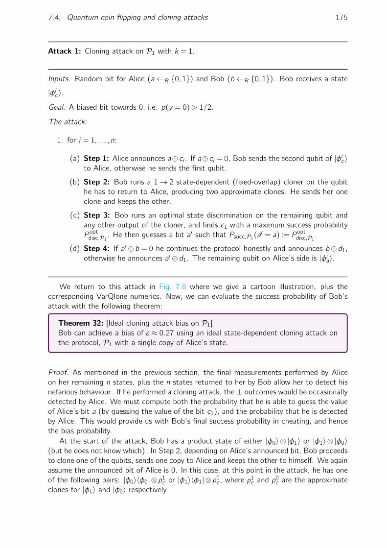
7.4. Quantum coin flipping and cloning attacks 175
Attack 1: Cloning attack on P1 with k = 1.
Inputs. Random bit for Alice (a←R 0,1) and Bob (b←R 0,1). Bob receives a state
|φic〉.
Goal. A biased bit towards 0, i.e. p(y = 0)> 1/2.
The attack:
1. for i = 1, . . . ,n:
(a) Step 1: Alice announces a⊕ci . If a⊕ci = 0, Bob sends the second qubit of |φic〉to Alice, otherwise he sends the first qubit.
(b) Step 2: Bob runs a 1→ 2 state-dependent (fixed-overlap) cloner on the qubithe has to return to Alice, producing two approximate clones. He sends her oneclone and keeps the other.
(c) Step 3: Bob runs an optimal state discrimination on the remaining qubit andany other output of the cloner, and finds c1 with a maximum success probabilityP opt
disc,P1. He then guesses a bit a′ such that Psucc,P1
(a′ = a) := P optdisc,P1
.
(d) Step 4: If a′⊕b = 0 he continues the protocol honestly and announces b⊕d1,otherwise he announces a′⊕d1. The remaining qubit on Alice’s side is |φia〉.
We return to this attack in Fig. 7.8 where we give a cartoon illustration, plus thecorresponding VarQlone numerics. Now, we can evaluate the success probability of Bob’sattack with the following theorem:
Theorem 32: [Ideal cloning attack bias on P1]Bob can achieve a bias of ε≈ 0.27 using an ideal state-dependent cloning attack onthe protocol, P1 with a single copy of Alice’s state.
Proof. As mentioned in the previous section, the final measurements performed by Aliceon her remaining n states, plus the n states returned to her by Bob allow her to detect hisnefarious behaviour. If he performed a cloning attack, the ⊥ outcomes would be occasionallydetected by Alice. We must compute both the probability that he is able to guess the valueof Alice’s bit a (by guessing the value of the bit c1), and the probability that he is detectedby Alice. This would provide us with Bob’s final success probability in cheating, and hencethe bias probability.
At the start of the attack, Bob has a product state of either |φ0〉⊗ |φ1〉 or |φ1〉⊗ |φ0〉(but he does not know which). In Step 2, depending on Alice’s announced bit, Bob proceedsto clone one of the qubits, sends one copy to Alice and keeps the other to himself. We againassume the announced bit of Alice is 0. In this case, at this point in the attack, he has oneof the following pairs: |φ0〉〈φ0|⊗ρ1
c or |φ1〉〈φ1|⊗ρ0c , where ρ
1c and ρ0
c are the approximateclones for |φ1〉 and |φ0〉 respectively.

176 7. Practical quantum cryptanalysis by variational quantum cloning
Bob must now discriminate between the following density matrices:
ρ1 := |φ0〉〈φ0|⊗ |φ1〉〈φ1| and ρ2 := |φ1〉〈φ1|⊗ρ0c (7.68)
Alternatively, if Alice announced a⊕ci = 1, he would have:
ρ1 := |φ1〉〈φ1|⊗ |φ0〉〈φ0| and ρ2 := |φ0〉〈φ0|⊗ρ1c (7.69)
In either case, we have that the minimum discrimination error for two density matrices isgiven by the Holevo-Helstrom bound [Hol73, Hel69] as follows14:
P optdisc =
1
2+
1
4||ρ1−ρ2||Tr =
1
2+
1
2dTr(ρ1,ρ2) (7.70)
The ideal symmetric cloning machine for these states will have an output of the form:
ρc = α|φ0〉〈φ0|+β|φ1〉〈φ1|+γ(|φ0〉〈φ1|+ |φ1〉〈φ0|) (7.71)
Where α,β and γ are functions of the overlap s = 〈φ0 |φ1〉= cos π9 . Now, using Eq. (7.68),ρ2 can be written as follows:
ρ2 = α|φ1〉〈φ1|⊗ |φ0〉〈φ0|+β|φ1〉〈φ1|⊗ |φ1〉〈φ1|+γ(|φ1〉〈φ1|⊗ |φ0〉〈φ1|+ |φ1〉〈φ1|⊗ |φ1〉〈φ0|) (7.72)
Finally by plugging in the values of the coefficients in Eq. (7.71) for the optimal localcloning machine [BDE+98] and finding the eigenvalues of σ := (ρ1−ρ2), we can calculatethe corresponding value for Eq. (7.70), and recover the following minimum error probability:
Pfail,P1= P er
disc,P1= 1−P opt
disc,P1≈ 0.214 (7.73)
This means that Bob can successfully guess c1 with P 1succ,P1
= 78.5% probability.Now let us examine the probability of a cheating Bob being detected by Alice. We
note that whenever Bob guesses the bit, a, successfully, the measurements (Eb,E⊥b ) will
be passed with probability 1, hence we use (Ea,E⊥a ) where the states sent by Bob will be
measured. Using Eq. (2.88) with the value of overlap s = cos(π/9), the optimal fidelityis FL ≈ 0.997 and so the probability of Bob getting caught is at most 1%. Putting thistogether with Bob’s guessing probability for a gives his overall success probability of 77.5%.
In the end, this implies that Bob is able to successfully create a bias of ε≈ 0.775−0.5 =
0.275.
We also have the following corollary, for a general number of states (n) exchanged,which shows the protocol can be completely broken and Bob can enforce an arbitrary bias:
Corollary 5: The probability of Bob successfully guessing a over all n copies has theproperty:
limn→∞
P nsucc,P1= 1 (7.74)
14This also is because the we assume a symmetric cloning machine for both |φ0〉 and |φ1〉. If this is notthe case, the guessing probability is instead the average of the discrimination probabilities over both states.

7.4. Quantum coin flipping and cloning attacks 177
Proof. If Bob repeats Attack 1 over all n copies, he will guess n different bits a′ini=1. Hecan then take a majority vote and announce b such that a∗⊕b = 0, where we denote a∗ asthe bit he guesses in at least n
2 + 1 of the rounds.If n is even, he may have guessed a′ to be 0 and 1 an equal number of times. In this case,
the attack becomes indecisive and Bob is forced to guess at random. Hence we separatethe success probability for even and odd n as follows:
P nsucc,P1=
n
∑
k= n+12
(nk
)(1−Pfail)
kP n−kfail n odd,
n
∑k= n
2 +1
(nk
)(1−Pfail)
kP n−kfail + 12
(nn/2
)(1−Pfail)
n2P
n2
fail n even(7.75)
By substituting the value of Pfail one can see that the function is uniformly increasing withn so lim
n→∞P nsucc,P1
= 1.
Although as Bob’s success probability in guessing correctly increases with n, the proba-bility of his cheating strategy getting detected by Alice will also increase. We also note thatthis strategy is independent of k , the number of different bits used during the protocol.
7.4.3 4-state coin flipping protocol (P2)
Another class of coin flipping protocols are those which require all the four states in Eq.(7.65). One such protocol was proposed by Aharonov et al. [ATSVY00], where φ is set asπ8 :
|φx,a〉=
|π8 x,0〉= cos
(π8
)|0〉+ (−1)x sin
(π8
)|1〉
|π8 x,1〉= sin(π8
)|0〉+ (−1)x⊕1 cos
(π8
)|1〉
(7.76)
In protocols of this form, Alice encodes her bit in ‘basis information’ of the family ofstates. For instance, we can take |φ0,0〉, |φ1,0〉 to encode the bit a= 0 and |φ0,1〉, |φ1,1〉to encode a = 1. The goal again is to produce a final ‘coin flip’ y = a⊕b, while ensuringthat no party has biased the bit, y . A similar protocol has also been proposed using BB84states [BB14] where |φ0,0〉 := |0〉, |φ0,1〉 := |1〉, |φ1,0〉 := |+〉 and |φ1,1〉 := |−〉. In this case,the states (also some protocol steps) are different but the angle between them is the sameas those in P2. A fault-tolerant version of P2 has also been proposed in [BBBG09], whichuses a generalised angle as in Eq. (7.65).
The protocol proceeds as follows. First Alice sends one of the states, |φx,a〉 to Bob.Later, one of two things will happen. Either, Alice sends the bits (x,a) to Bob, whomeasures the qubit in the suitable basis to check if Alice was honest, or Bob is asked toreturn the qubit |φx,a〉 to Alice, who measures it and verifies if it is correct. Now, examplecheating strategies for Alice involve incorrect preparation of |φx,a〉 and giving Bob the wronginformation about (x,a), or for Bob in trying to determine the bits (x,a) from |φx,a〉 beforeAlice has revealed them classically. We again focus only on Bob’s strategies here to usecloning arguments. We note that the information theoretic achievable bias of ε = 0.42
proven in [ATSVY00] applies only to Alice’s strategy since she has greater control of theprotocol (she prepares the original state). In general, a cloning based attack strategy byBob will be able to achieve a lower bias, as we show. As above, Bob randomly selects hisown bit b and sends it to Alice. He then builds a QCM to clone all 4 states in Eq. (7.76).

178 7. Practical quantum cryptanalysis by variational quantum cloning
We next sketch the two cloning attacks on Bob’s side of P2. Again, as with the protocol,P1, Bob can cheat using as much information as he gains about a and again, once Bob hasperformed the cloning, his strategy boils down to the problem of state discrimination. Inboth attacks, Bob will use a (variational) state-dependent cloning machine.
7.4.3.1 Cloning attacks on P2
In the first attack model (which we denote I - see Fig. 7.9(a) in Sec. 7.5.3) Bob measures allthe qubits outputted from the cloner to try and guess (x,a). As such, it is the global fidelitythat will be the relevant quantity. This strategy is useful with the first possible challengein the protocol, where Bob is not required to send anything back to Alice. We discuss inAppendix 7.4.3.2 how the use of cloning in this type of attack can also reduce resources forBob from a general POVM to projective measurements in the state discrimination, whichmay be of independent interest. The main attack here boils down to Bob measuring theglobal output state from his QCM using the projectors, |v〉〈v |, |v⊥〉〈v⊥ |, and from thismeasurement, guessing a. These projectors are constructed explicitly relative to the inputstates using the Neumark theorem [BK15].
The second attack model (which we denote II, see Fig. 7.9(a) in Sec. 7.5.3) is instead alocal attack and as such will depend on the optimal local fidelity. It may also be more relevantin the scenario where Bob is required to return a quantum state to Alice. We note thatBob could also apply a global attack in this scenario but we do not consider this possibilityhere in order to give two contrasting examples. In the below, we compute a bias assuminghe does not return a state for Alice for simplicity and so the bias will be equivalent to hisdiscrimination probability. The analysis could be tweaked to take a detection probability forAlice into account also. In this scenario, Bob again applies the QCM, but now he only usesone of the clones to perform state discrimination (given by the Discriminator in Fig. 7.9(a)).
7.4.3.2 Attack I on P2
For attack I, which is a 4 state global attack on P2, we have:
Theorem 33: [Ideal cloning attack (I) bias on P2]Using a cloning attack on the protocol, P2, (in attack model I) Bob can achieve abias:
εIP2,ideal ≈ 0.35 (7.77)
We note first that this attack model (i.e. using cloning) can be considered a constructiveway of implementing the optimal discrimination strategy of the states Alice is to send. Inorder to bias the bit, Bob needs to discriminate between the four pure states in Eq. (7.65)or equivalently between the ensembles encoding a= 0,1, where the optimal discriminationis done via a set of POVM measurements.
However, by implementing a cloning based attack, we can simplify the discrimination.This is because the symmetric state-dependent cloner (which is a unitary) has the inter-esting feature that for either case (a = 0 or a = 1), the cloner’s output is a pure statein the 2-qubit Hilbert space. As such, the states (after going through the QCM) can beoptimally discriminated via a set of projective measurements Pv ,Pv⊥, rather than generalPOVMs (as would be the case if the QCM was not used). So, using VarQlone to obtain

7.4. Quantum coin flipping and cloning attacks 179
optimal cloning strategies also is a means to potentially reduce resources for quantum statediscrimination also. Now, let us prove Theorem 33:
Proof. The attack involves the global output state of the cloning machine. For this attackwe can use the fixed overlap 1→ 2 cloner with the global fidelity given by Eq. (2.89):
F FO,optG (1,2) =
1
2
(1 + s3 +
√1− s2
√1− s4
)≈ 0.983 (7.78)
where s = sin(2φ) = cos(π4 ) for P2. Alternatively we can use the 4-state cloner which clonesthe two states with a fixed overlap plus their orthogonal set. For both of these cloners weare interested in the global state of the cloner which we denote as |ψ1→2
x,a 〉 for an input state|φx,a〉.
In order for Bob to guess a he must discriminate between |φ0,0〉 (encoding a = 0) and|φ1,1〉 (encoding a = 1) or alternatively the pair |φ0,1〉, |φ1,0〉. This is since the pairs|φ0,0〉, |φ0,1〉 are orthogonal and |φ0,0〉, |φ1,0〉 both encode a = 0, so the only choice isto discriminate between |φ0,0〉 and |φ1,1〉. Due to the symmetry and without an ancilla, thecloner preserves the overlap between each pairs i.e. 〈ψ1→2
0,0 |ψ1→21,1 〉 = 〈φ0,0 |φ1,1〉 = s (we
also have 〈ψ1→20,1 |ψ1→2
1,0 〉= s).Now we select the projective measurements Pv = |v〉〈v | and Pv⊥ = |v⊥〉〈v⊥| such that〈v |v⊥〉= 0. One can show that the discrimination probability is optimal when |v〉 and |v⊥〉are symmetric with respect to the target states (illustrated in Fig. 7.9(a)) according to theNeumark theorem. From the figure, we have that 〈v |v⊥〉= 0 so 2θ+ 2φ= π
2 ⇒ θ = π4 −φ.
Finally, writing the cloner’s states for |ψ1→20,0 〉, |ψ1→2
1,1 〉 in the basis |v〉, |v⊥〉 gives:
|ψ1→20,0 〉= cos
(π4−φ)|v〉+ sin
(π4−φ)|v⊥〉,
|ψ1→21,1 〉= cos
(π4−φ)|v〉− sin
(π4−φ)|v⊥〉
(7.79)
where it can be checked that 〈ψ1→20,0 |ψ1→2
1,1 〉 = cos(π2 −2φ
)= sin(2φ) = s. Hence |v〉 and
|v⊥〉 can be explicitly derived. Note that these bases are also symmetric with respect tothe other pair i.e |ψ1→2
0,1 〉, |ψ1→21,0 〉. Finally, the success probability of this measurement is
then given by:
P opt,Idisc,P2
=1
2+
1
2〈ψ1→2
0,0 |ψ1→21,1 〉=
1
2+
1
2sin2φ= 0.853 (7.80)
which is the maximum cheating probability for Bob. From this, we derive the bias as:
εIP2,ideal = P opt,I
disc,P2−
1
2= 0.353 (7.81)
which completes the proof.
7.4.3.3 Attack II on P2
Finally, we consider a second attack model (attack II) on the protocol, P2, which is in theform of a ‘local’ attack. Here, we further consider two scenarios:
1. A cloning machine which is able to clone all 4 states: |φ0,0〉, |φ1,1〉 and |φ0,1〉, |φ1,0〉,

180 7. Practical quantum cryptanalysis by variational quantum cloning
2. A cloning machine tailored to only the two states, |φ0,0〉 and |φ1,1〉 (which Bob needsto discriminate between).
We focus on the former scenario, since it connects more cleanly with the VarQlone clonefidelities, but scenario 2 facilitates a more optimal attack (in the ideal situation).
Scenario 1:
In this case, we can compute an exact discrimination probability, but it will result in aless optimal attack.
Theorem 34: [Ideal cloning attack (II) bias on P2 in scenario 1.]Using a cloning attack on the protocol, P2, (in attack model II with 4 states) Bobcan achieve a bias:
εIIP2,ideal = 0.25 (7.82)
As a sketch proof, we explicitly evaluate the output states from an ideal cloner, and thencompute the success probability via the trace distance. The full proof for this theorem isgiven in Appendix A.2.7.
Scenario 2:
Here, we give a bound on the success probabilities of Bob in terms of the local fidelitiesof the QCM where the cloning machine is only tailored to clone two fixed-overlap states.Here we rely on the fact that Bob can discriminate between the two ensembles of states(for a = 0, a = 1) with equal probabilities.
Theorem 35: The optimal discrimination probability for a cloning attack on the pro-tocol, P2, (in attack model II, with 2 states) is:
0.6196 P opt,IIdisc,P2
6 0.823 (7.83)
Proof. For each of the input states, |φi ,j〉, in Eq. (7.76), we denote ρci j to be a cloneoutputted from the QCM. Due to symmetry, we only need to consider one of the twooutput clones. We can now write the effective states for each encoding (a = 0,a = 1) as:
ρ(a=0) :=1
2(ρc00 +ρc10), ρ(a=1) :=
1
2(ρc01 +ρc11) (7.84)
Dealing with these two states is sufficient since it can be shown that discriminating betweenthese two density matrices, is equivalent to discriminating between the entire set of 4 statesin Eq. (7.65).
Again, we use the discrimination probability from the Holevo-Helstrom bound:
P opt,IIdisc,P2
:= P optdisc(ρ(a=0),ρ(a=1)) :=
1
2+
1
2dTr(ρ(a=0),ρ(a=1)) (7.85)

7.4. Quantum coin flipping and cloning attacks 181
Now, we have:
dTr(ρ(a=0),ρ(a=1)) =1
2
∣∣∣∣ρ(a=0)−ρ(a=1)
∣∣∣∣Tr
=1
2
∣∣∣∣∣∣∣∣12(ρc00−ρc11) +1
2(ρc10−ρc01)
∣∣∣∣∣∣∣∣Tr
61
4||(ρc00−ρc11)||Tr + ||(ρc10−ρc01)||Tr
61
2[dTr(ρ
c00,ρ
c11) +dTr(ρ
c01,ρ
c10)]
=⇒ P optdisc(ρ(a=0),ρ(a=1))6
1
2(P opt
disc(ρc00,ρc11) +P opt
disc(ρc01,ρc10))
= P optdisc(ρc00,ρ
c11)
(7.86)
The last equality follows since for both ensembles, |φ0,0〉, |φ1,1〉 and |φ0,1〉, |φ1,0〉, theiroutput clones have equal discrimination probability:
P optdisc(ρc00,ρ
c11) = P opt
disc(ρc01,ρc10) (7.87)
This is because the QCM is symmetric, and depends only on the overlap of the states (wehave in both cases 〈φ00 |φ11〉= 〈φ01 |φ10〉= sin(2φ)).
Furthermore, since the cloning machine can only lower the discrimination probabilitybetween two states, we have:
P optdisc(ρc00,ρ
c11)6 P opt
disc(ρc00, |φ1,1〉〈φ1,1|) =: P optdisc
Now, using the relationship between fidelity and the trace distance (Eq. (2.73)), we havethe bounds:
1
2+
1
2
(1−√〈φ1,1|ρc00|φ1,1〉
)6 P opt
disc 61
2+
1
2
√1−〈φ1,1|ρc00|φ1,1〉 (7.88)
By plugging in the observed density matrix for the output clone, we can find this discrimi-nation probability. As in the previous section, the output density matrix from the QCM foran output clone can be written as Eq. (7.71):
ρc00 = α|φ0,0〉〈φ0,0|+β|φ1,1〉〈φ1,1|+γ(|φ0,0〉〈φ1,1|+ |φ1,1〉〈φ0,0|) (7.89)
This state has a local fidelity, FL = 〈φ0,0|ρc00|φ0,0〉= α+ s2β+ sγ. On the other hand, wehave F (ρc00, |φ1,1〉〈φ1,1 |) = s2α+β+ sγ.
Combining these two, we then have:
F (ρc00, |φ1,1〉〈φ1,1 |) = FL + (s2−1)(α−β) (7.90)
Plugging in FL from Eq. (2.88), and α− β =√
1−s2
1−s4 (for an optimal state-dependentcloner), we get:
1
2+
1
2
1−
√FL + (s2−1)
√1− s2
1− s4
6 P opt,IIdisc,P2
61
2+
1
2
√1−FL− (s2−1)
√1− s2
1− s4(7.91)
To complete the proof, we use FL ≈ 0.989 and s = 1/√
2 which gives the numerical dis-crimination probabilities above.

182 7. Practical quantum cryptanalysis by variational quantum cloning
7.5 VarQlone numerics
In preceding sections, we introduced the VarQlone algorithm and its relationship to cryp-tography at a high level. We also introduced (theoretical) cryptographic attacks on severalprotocols. Here, we combine these two aspects and present the corresponding numericalresults.
Before diving back into the cryptographic applications, let us revisit some specifics ofthe VarQlone algorithm, in particular the ansätze we use.
The first two options are fixed-structure ansätze. We include one which is ‘problem-inspired’ (based on the theoretical derivation) and one which is ‘problem-agnostic’ (a hardware-efficient fixed-structure (HEFS)) using the nomenclature of Sec. 4.1.2. We then generaliseto the primary one we opt for, a variable-structure ansatz. Recall, in the latter case, boththe continuous parameters and the gates in the ansatz are optimised over (see Sec. 4.1.2).
7.5.1 Fixed-structure ansätze
To demonstrate the fixed-structure ansätze, we use 1→ 2 phase-covariant cloning as theprimary example (recall this is the relevant cloning family to attack the BB84 protocol),which requires cloning the following states:
|ψxy (η)〉=1√2
(|0〉+e iη|1〉
)(7.92)
7.5.1.1 Phase-covariant cloning with a fixed ideal ansatz
Let us begin with a problem-inspired option. Recall, the ideal circuit for performing phase-covariant cloning is given by Fig. 2.4. Here, we learn the parameters of this fixed circuit.This gives us the opportunity to illustrate the effect of measurement noise in using the SWAPtest. The results of this can be seen in Fig. 7.4. We compare the SWAP test in Fig. 7.4(a)to ‘direct simulation’ in Fig. 7.4 (b) to compute the fidelities. Direct simulation hererefers to the explicit extraction of a classical description of the qubit density matrices.We do this using quantum state tomography [DPS03] with the forest-benchmarkinglibrary [GCH+19]. Note, that this intermediate step via tomography is not necessary ingeneral as with sufficiently low hardware noise, the fidelity could be directly extracted viathe an overlap test (i.e., the SWAP test). The effect of measurement noise can be clearlyseen in the latter case.
We note in the main text that we do not use the SWAP test when running the exper-iments on the Aspen QPU. This is because the test fails to output the fidelity since bothstates to compare will be mixed due to device noise. However, this essentially reproducesthe findings of [JJB+19] in a slightly different scenario. Furthermore, this was only possiblebecause we had prior knowledge of an optimal circuit to implement the cloning transforma-tion from [BBHB97, FWJ+14]. Of course, in generality this information is not available,which precludes the use of (problem-inspired) fixed-structure ansätze.
7.5.1.2 Phase-covariant cloning with a hardware-efficient fixed ansatz
Let us now test the problem-agnostic hardware-efficient fixed-structure (HEFS) ansatz forthe sample problem as in the previous section. Here, we introduce a number of layers in the
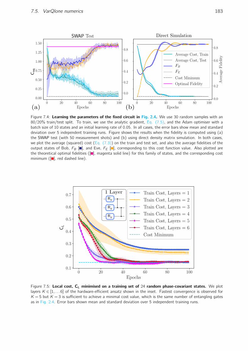
7.5. VarQlone numerics 183
Figure 7.4: Learning the parameters of the fixed circuit in Fig. 2.4. We use 30 random samples with an80/20% train/test split. To train, we use the analytic gradient, Eq. (7.5), and the Adam optimiser with abatch size of 10 states and an initial learning rate of 0.05. In all cases, the error bars show mean and standarddeviation over 5 independent training runs. Figure shows the results when the fidelity is computed using (a)the SWAP test (with 50 measurement shots) and (b) using direct density matrix simulation. In both cases,we plot the average (squared) cost (Eq. (7.3)) on the train and test set, and also the average fidelities of theoutput states of Bob, FB [ ], and Eve, FE [ ], corresponding to this cost function value. Also plotted arethe theoretical optimal fidelities ([ ], magenta solid line) for this family of states, and the corresponding costminimum ([ ], red dashed line).
Figure 7.5: Local cost, CL minimised on a training set of 24 random phase-covariant states. We plotlayers K ∈ [1, . . .6] of the hardware-efficient ansatz shown in the inset. Fastest convergence is observed forK = 5 but K = 3 is sufficient to achieve a minimal cost value, which is the same number of entangling gatesas in Fig. 2.4. Error bars shown mean and standard deviation over 5 independent training runs.

184 7. Practical quantum cryptanalysis by variational quantum cloning
ansatz, K, in which each layer has a fixed-structure. For simplicity, we choose each layerto have parametrised single qubit rotations, Ry (θ), and nearest neighbour CZ gates. Wedeal again with 1→ 2 cloning, so we use 3 qubits and therefore we have 2 CZ gates perlayer. We show the results for K = 1 layer to K = 6 layers in Fig. 7.5. Not surprisingly, weobserve convergence to the minimum as the number of layers increases, saturating at K = 3.
Barren Plateaus
Furthermore, we can examine VarQlone for the existence of barren plateaus in this scenario.Recall from Sec. 4.1.1, a local VQA cost can be written as:
CL = κTr[OLU(θ)ρU(θ)†
], (7.93)
OL = c01+∑j
cjOj (7.94)
Note that taking c0 = 1,cj = −1/N ∀j and κ = 1 recovers the specific form of our cost,Eq. (7.1). We will prove that this cost does not exhibit barren plateaus for a sufficientlyshallow alternating layered ansatz, i.e. U(θ) contains blocks, W , acting on alternating pairsof qubits [CSV+21]. To do so, we first recall the following Theorem from [CSV+21]:
Theorem 36: Consider a trainable parameter, θl in a block, W of an alternatinglayered ansatz (denoted U(θ)). Let Var[∂l C] be the variance of an m-local costfunction, C with respect to θl . If each block in U(θ) forms a local 2-design, thenVar[∂l C] is lower bounded by:
GN(K,k)6 Var[∂l C] (7.95)
GN(K,k) =2m(k+1)−1
(22m−1)2(2m + 1)K+k ∑j∈jL
∑(p,p′)∈pLBp′>p
χj(p,p′,Oj) (7.96)
χj(p,p′,Oj) := c2
j dHS
(ρp,p′,
Tr(ρp,p′)1
dρ(p,p′)
)dHS
(Oj ,
Tr(Oj)1
dOj
)(7.97)
jL are the set of j indices in the forward light-conea LB of the block W and ρp,p′ isthe partial trace of the input state, ρ, down to the subsystems Sp,Sp+1, . . . ,Sp′. dMdenotes the dimension of a matrix M and dHS denotes the Hilbert-Schmidt distancefrom Eq. (2.67).
aThe forward light-cone is the subset of qubits which are causally connected (in the future) to thequbit(s) on which the block W is applied.
Sp in the above represents the qubit subsystem in which W acts. Firstly, the operators

7.5. VarQlone numerics 185
Oj are all single qubit projectors (m = 1 local), |ψ〉〈ψ |, so we have:
dHS
(Oj ,Tr(Oj)
1
d
)= dHS
(|ψ〉〈ψ |,Tr [|ψ〉〈ψ |]
1
2
)(7.98)
=
√√√√Tr
[(|ψ〉〈ψ |−
1
2
)(|ψ〉〈ψ |−
1
2
)†](7.99)
=
√Tr
[|ψ〉〈ψ |−
|ψ〉〈ψ |2−|ψ〉〈ψ |
2+1
4
]=
√Tr
(1
4
)=
1√2
(7.100)
So G(K,k) simplifies to:
GN(K,k) =2k
3K+k+2√
2N2 ∑j∈jL
∑(p,p′)∈pLBp′>p
dHS
(ρp,p′,
1
dρ(p,p′)
)(7.101)
If we now define SP to be the subsystems from p to p′, the reduced state of ρ in SP willbe one of either |ψ〉〈ψ |⊗|P |, |0〉〈0 |⊗|P | or |ψ〉〈ψ |⊗q|0〉〈0 |⊗|P |−q for some q < |P | wherewe denote |P | to be the number of qubits in the reduced subsystem SP . Since these areall pure states, we can compute dHS(ρp,p′,1/dρ(p,p′)) =
√1−1/dρ(p,p′). Lower bounding the
sum over j by 1 and√
1−1/dρ(p,p′) by 1/√
2 (dρ(p,p′) is at least 2) gives:
2k
3K+k+22N26 GN(K,k) (7.102)
Finally, by choosing K ∈O (log(N)), we have that k,K+k ∈O(log(N)) and so Gn(K,k) ∈Ω(1/poly(N)). Since we have that if G(K,k) vanishes no faster than Ω(1/poly(N)), then sodoes the variance of the gradient and so will not require exponential resources to estimate.As a result, we can formalise the following corollary:
Corollary 6: [Absence of barren plateaus in local cost]Given the local VarQlone cost function, CL (Eq. (7.1)) in M → N cloning, and ahardware-efficient fixed-structure ansatz, U(θ), made up of alternating blocks, W ,with a depth O(log(N)), where each block forms a local 2-design. Then the varianceof the gradient of CL with respect to a parameter, θl can be lower bounded as:
GN := min(GN(K,k))6 Var[∂l C], GN(K,k) ∈Ω
(1
poly(N)
)(7.103)
One final thing to note, is that the ansatz we choose in Fig. 7.5, does not form an exactlocal 2-design, but the same ansatz is used in [CSV+21]) and is sufficient to exhibit a costfunction dependent barren plateau.

186 7. Practical quantum cryptanalysis by variational quantum cloning
7.5.2 Variable-structure ansätze
For our variable-structure ansatz, we adopt the approach of [CSSC18] which fixes thelength, l , of the circuit sequence to be used,contains parametrised single qubit gates, andun-parametrised entangling gates, which we chose to be CZ for simplicity. For example,with a three qubit chip, we have an example gatepool:
G = R0z(θ),R1
z(θ),R2z(θ),R0
x(θ),R1x(θ),R2
x(θ),
R0y (θ),R1
y (θ),R2y (θ),CZ0,1,CZ1,2,CZ0,2 (7.104)
We use the CZ gate as the entangler for two reasons. The first is that CZ is a nativeentangling gate on the Rigetti hardware. The second is that it simplifies our problemslightly, since it is symmetric on the control and target qubit, we do not need to worryabout the ordering of the qubits: CZi ,j = CZj,i . The unitary to be learned is given by:
Ug(θ) = Ug1(θ1)Ug2(θ2) . . .Ugl (θl) (7.105)
where each gate is from the above set G. The sequence, g := [g1, . . . ,gl ], in Eq. (4.12)and Eq. (7.105) above, corresponds to the indices of the gates in an ordered version of G.So using G in Eq. (7.104) as an example, g = [0,6,3,2,10] would give the unitary:
Ug(θ) = R0z(θ1)R1
y (θ2)R0x(θ3)R2
z(θ4)CZ0,1 (7.106)
and θ := [θ1,θ2,θ3,θ4,0].At the beginning of the procedure, the gate sequence is chosen randomly (, i.e. a random
sequence for the gate indices, g), and also the parameters (θ) therein15.The optimisation procedure proceeds over a number of epochs and iterations. In each
iteration, g is perturbed by altering d gates, giter→ giter+1, so giter+1 has at most dgates different from giter. The probability of changing d gates is given by 1/2d , and theprobability of doing nothing (i.e. giter = giter+1) is:
Pr(d = 0) = 1−l
∑d=1
1
2d= 2−
1− 12l
1− 12
−1
2l(7.107)
The epochs correspond to optimisation of the parameters θ using the Adam optimiser (Eq.(3.8)). We typically set the maximum number of epochs to be 100 and iterations to be50 in all this work. After each iteration, the best cost, Cbest
t for a chosen cost - eitherthe local, Eq. (7.1) (t = L), the global, Eq. (7.4) (t = G), squared, Eq. (7.3) (t = sq)or some other choice, is updated, if that iteration has found a circuit with a lower cost.As in [CSSC18], we repeatedly compress the sequence by removing redundant gates (e.g.combining Ugi (θi) and Ugi+1
(θi+1) if gi = gi + 1), and adding random gates to keep thesequence length fixed at gl .
Fig. 7.6 illustrates some results from this protocol. We find that with an increasingsequence length, the procedure is more likely to find circuits which achieve the minimumcost, and is able to first do so with a circuit with between 25-30 gates from the abovegateset in Eq. (7.108). We also plot the results achieved in a particular run of the protocol
15If some information is known about the problem beforehand, this could be used to initialise the sequenceand improve performance.

7.5. VarQlone numerics 187
Figure 7.6: Variable-structure ansatz details for VarQlone. (a) CbestL as a function of sequence length, l in
achieving the same task as Fig. 2.4, where the Bob and Eve’s clones appear in qubits 1 and 2. As l increases,the number of runs which successfully approach the theoretical minimum increases. Error bars shown meanand standard deviations for the minimum costs achieved over 20 independent runs with each sequence length.(b) Cost achieved for 50 iterations of the structure learning protocols, using a sequence length of l = 35.Recall an iteration is an update to the circuit structure, whereas an epoch is an update to the circuitparameters. Each line (iteration) corresponds to a slightly different circuit structure, g. Early iterations(darker lines) are not able to find the minimum, but eventually, a circuit is found which has this capacity. Foreach g, θ is trained for 100 epochs of gradient descent, using the Adam optimiser. If an iteration has notconverged close enough to Cbest
L by 30 epochs, the iteration is ended.
in Fig. 7.6(b). Here, an ‘iteration’ is an update to the circuit structure, whereas an‘epoch’ is an update to the circuit parameters (as in previous chapters). As the circuitlearns, it is able to subsequently lower Cbest
t , until it eventually finds a circuit capable ofachieving the optimal cost for the problem.
7.5.2.1 Phase-covariant cloning
Now, we return to phase-covariant cloning, and implement the procedure detailed above16.We consider this to be the proof of principle implementation of our methods. The results ofthis can be seen in Fig. 7.7. Let us begin by describing some problem parameters. Firstly,we allow 3 qubits (2 output clones plus 1 ancilla) in the circuit. Next, we give the VarQlonethe following fully connected (FC) gateset pool for this problem (indices represent qubits ofthe Aspen-8 sublattice):
GPC = R2z(θ),R3
z(θ),R4z(θ),R2
x(θ),R3x(θ),R4
x(θ),
R2y (θ),R3
y (θ),R4y (θ),CZ2,3,CZ3,4,CZ2,4 (7.108)
Let us now discuss in greater detail the observations which can be drawn from Fig. 7.7.Here, Fig. 7.7(c, d) illustrates some candidate cloning circuits learned by VarQlone, com-pared to the optimal ‘analytic’ circuit (the same one from Fig. 2.4) given in [BBHB97,FMWW01, FWJ+14] (Fig. 7.7(b)).
We being by noting that all three circuits approximately saturate the optimal bound forphase-covariant cloning (FL = 0.85, which is plotted as a red dotted line in Fig. 7.7) when
16For all results shown using a variable-structure ansatz, we use the forest-benchmarking li-brary [GCH+19] to reconstruct the output density matrix (and from this quantity then compute the overlapsand fidelities required) in order to mitigate the effect of quantum noise

188 7. Practical quantum cryptanalysis by variational quantum cloning
Figure 7.7: Variational quantum cloning implemented on phase-covariant states using three qubits ofthe Rigetti Aspen-8 chip (QPU), plus simulated results (QVM). Violin plots in (a) show the cloningfidelities, for Bob and Eve, found using each of the circuits shown in (b)–(d) respectively. Shown in red isthe maximal possible fidelity for this problem. (b) is the ideal circuit with clones appearing in registers 2 and3 [ , ]. (c) shows the structure-learned circuit for the same scenario, using one less entangling gate [ , ].(d) demonstrates the effect of allowing clones to appear in registers 1 and 2 [ , ]. In the latter case, onlyfour (nearest-neighbour) entangling gates are used, demonstrating a significant boost in performance on theQPU. In all cases the fidelity is extracted explicitly using quantum state tomography, as discussed in the text.
simulated (i.e. without quantum noise).Next, we move to performance on the actual hardware, the Aspen-8 chip. We first notice
that the ideal circuit in Fig. 7.7(b) suffers a degradation in performance when implementedon the QPU since it requires 6 entangling gates to transfer the information across the circuit.Furthermore, since the Aspen-8 chip does not have any 3 qubit loops in its topology, it isnecessary for the compiler to insert SWAP gates, further reducing the quality of the clones.
The two examples for our learned circuits Fig. 7.7(c, d) are trained under two differentrestrictions. First, to ensure a fair comparison to the ideal circuit, we begin by forcing thequbit clones to appear in registers 2 and 3 of the circuit, (demonstrated in Fig. 7.7(c))exactly as in Fig. 7.7(b). Secondly, we allow the clones to appear instead in registers 1
and 2 (demonstrated in Fig. 7.7(d) - The circuit labelled ‘Rev.’ (‘Reverse’).) The abilityto make such a subtle change clearly demonstrates the advantage of our flexible approach.We notice that the restriction imposed in Fig. 7.7(c) results in only a modest performanceimprovement over the ideal. However, by allowing the clones to appear in registers 1 and2, VarQlone is able to find much more conservative circuits, having fewer entangling gates,and are directly implementable on a linear topology. This gives a significant improvementin the cloning fidelities, of about 15% when the circuit is run on the Aspen-8 QPU.
Now, let us return to discussing phase-covariant cloning through the lens of an adversaryeavesdropping on the BB84 protocol. We specifically analyse the performance of one ofthese VarQlone-learned circuits (Circuit(c)) in such an attack. We will do so by computingthe corresponding critical error rate, Dcrit, via the expression for the key rate, R, in Eq.(7.62) (recall the discussion in Sec. 7.3.1) for the BB84 protocol protocol run in X-Y Paulibasis.
We compute this for the circuit in Fig. 7.7(c) only, since while the circuit in Fig. 7.7(d)achieves higher fidelities on the Aspen hardware, it does not actually make use of the ancillaryqubit (the sequence of gates acting on it approximately resolve to the identity).

7.5. VarQlone numerics 189
Now, we compute the resulting mixed states outputted over all input states to thecloning machine, for each basis state: |+〉, |−〉, |+ i〉, |− i〉 so ρE in Eq. (7.63) is given by:
ρE :=1
4(ρ+E +ρ−E +ρ+i
E +ρ−iE ) (7.109)
Similarly, ρ0E,ρ
1E in Eq. (7.63) are the mixed states encoding the symbol 0 (which have
input |+〉, |+ i〉) and the symbol 1 (which have input |−〉, |− i〉), so are given by:
ρ0E :=
1
2(ρ+E +ρ+i
E ) ρ1E :=
1
2(ρ−E +ρ−i
E ) (7.110)
Calculating the minimum Holevo quantity (denoted by χmin) for the above density matricesoutputted by the circuit in Fig. 7.7(c) numerically gives the following:
1−H(Dcrit)−χmin = 0
⇒ 1−χmin + (Dcrit log2Dcrit + (1−Dcrit) log2 (1−Dcrit)) = 0
⇒Dcrit = 15.8%
(7.111)
which is very close to the optimal bound for the individual attack. Nevertheless as pointedout in [SIGA05, FL12], the same bound can be reached by a collective attack (where Evedefers any measurements until the end of the reconciliation phase, and applies a generalstrategy to all collected states) where the individual quantum operations are still given by theoptimal phase-covariant cloner. As such, the VarQlone learned attack can almost saturatethe optimal collective bound as well.
Finally, one may observe that Circuit (d) in Fig. 7.7 achieves a higher still fidelity onhardware, but it does so by not using the ancilla to reduce the circuit depth. As such, it isa better circuit for purely performing cloning than either (c) or (d), but does not provide anoptimal attack for BB84 [SIGA05].
Local versus Global Fidelities
As a final remark on this experiment, we can investigate the difference between theglobal and local fidelities achieved by the circuits VarQlone (i.e. in Fig. 7.7(c)) finds, versusthe ideal one (shown in Fig. 7.7(b)). Recall that in Sec. 7.2.4.4, we showed that the ‘ideal’circuit achieves both the optimal local and global fidelities for this problem:
F ig. 7.7(b) =⇒
F(b)B = F
(b)E = F opt
L = 12
(1 + 1√
2
)≈ 0.853
F(b)G = F opt
G = 18
(1 +√
2)2 ≈ 0.72
(7.112)
In contrast, our learned circuit (Fig. 7.7(c)) maximises the local fidelity, but in order to gainan advantage in circuit depth, compromises with respect to the global fidelity:
F ig. 7.7(c) =⇒
F
(c)B ≈ F (c)
E ≈ F optL = 0.85
F(c)G ≈ 0.638< F opt
G
(7.113)
7.5.3 State-dependent cloning
Next, let us move onto the results of VarQlone when learning to clone the states used inthe two coin flipping protocols described in Sec. 7.3. Firstly, we focus on the states used

190 7. Practical quantum cryptanalysis by variational quantum cloning
Figure 7.8: Overview of cloning-based attack on the protocol of Mayers et. al. [MSCK99], plus cor-responding numerical results for VarQlone. (a) Cartoon of coin flipping protocols, Alice and Bob sendquantum (q) and/or classical (c) information to agree on a final ‘coin flip’ bit, y . (b) The relevant part of theprotocol of Mayers et. al., P1, plus a cloning based attack on Bob’s side. He builds a cloning machine usingVarQlone to produce two clones of Alice’s sent states, one of which he returns, and the other is used to guessAlice’s input bit, a. (c) Fidelities of each output clone, ρjθ achieved using VarQlone when (1→ 2) cloning thefamily of states used in, P1. In the left (right) panel, |φ0〉 (|φ1〉) is. Figure shows both simulated (QVM -[ ] purple circles) and on Rigetti hardware (QPU - [ ] blue crosses). For the QVM (QPU) results, 256 (5)samples of each state are used to generate statistics. Violin plots show complete distribution of outcomesand error bars show the means and standard deviations. Inset (i) shows the two qubits of the Aspen-8 chipwhich were used, with the allowed connectivity of a CZ between them. Note an ancilla was also allowed, butVarQlone chose not to use it in this example. The corresponding learned circuit is given in Sec. 7.6.
in the original protocol, P1 for 1→ 2 cloning, and then move to the 4 state protocol, P2.In the latter we also extend from 1→ 2 cloning to 1→ 3 and 2→ 4. These extensions willallow us to probe certain features of VarQlone, in particular explicit symmetry in the costfunctions. In all cases, we use the variable-structure Ansatz, and once a suitable candidatehas been found, the solution is manually optimised further. The learned circuits used toproduce the figures in this section are given in Sec. 7.6.
7.5.3.1 Cloning P1 states
As a reminder, the two states used in this protocol are:
|φ0〉 := |φ0,0〉= cos( π
18
)|0〉+ sin
( π18
)|1〉 (7.114)
|φ1〉 := |φ0,1〉= cos( π
18
)|0〉− sin
( π18
)|1〉 (7.115)
The fidelities achieved by the VarQlone learned circuit can be seen in Fig. 7.8 using thegate pool Eq. (7.116) which allows a linear entangling connectivity:
GP1→21
:=Rij(θ),CZ2,3,CZ3,4
,∀i ∈ 2,3,4,∀j ∈ x,y ,z (7.116)
A deviation from the optimal fidelity is observed in the simulated case, partly due totomographic errors in reconstructing the cloned states. We note that the correspondingcircuit for Fig. 7.8 only actually used 2 qubits (see Sec. 7.6). This is because while VarQlone
7.5. VarQlone numerics 191
was allowed to use the ancilla, it chose not in this case by applying only identity gates toit. This mimics the behavior seen in the previous example of phase-covariant cloning. Assuch, we only use the two qubits shown in the inset (i) of the figure when running on theQPU to improve performance.
Now, returning to the attack on P1 above, we can compute the success probabilitiesusing these fidelities. For illustration, let us return to the example in Eq. (7.68), whereinstead the cloned state is now produced from our VarQlone circuit, ρ0
c → ρ0VarQlone.
Theorem 37: [VarQlone attack bias on P1]Bob can achieve a bias of ε≈ 0.29 using a state-dependent VarQlone attack on theprotocol, P1, with a single copy of Alice’s state.
We can prove Theorem 37 by computing the success probability in the same manner aswas done in Sec. 7.4.2:
PVarQlonesucc,P1
=1
2+
1
4Tr|ρ1−|φ1〉〈φ1|⊗ρ0
VarQlone| ≈ 0.804 (7.117)
The state ρ1 = |φ0〉〈φ0|⊗ |φ1〉〈φ1| as in Eq. (7.68). Here, we have a higher probability forBob to correctly guess Alice’s bit, a, but correspondingly the detection probability by Aliceis higher than in the ideal case, due to a marginally lower local fidelity of FVarQlone
L = 0.985.
7.5.3.2 Cloning P2 states.
Next, we turn to the family of states used in the 4 states protocol, given by Eq. (7.76):
1→ 2 Cloning
Firstly, we repeat the exercise from above with the same scenario, using the same gatesetand subset of the Aspen-8 lattice (GP1→2
2= GP1→2
1). We use the local cost, Eq. (7.1), to
train the model, with a sequence length of 35 gates. The results are seen in Fig. 7.9(b)both on the QVM and the QPU. We note that the solution exhibits some small degree ofasymmetry in the output states, due to the form of the local cost function. This asymmetryis especially pronounced as we scale the problem size and try to produce N output clones,which we discuss in the next section.
Now, we can relate the performance of the VarQlone cloner to the attacks discussedin Sec. 7.4.3. We do this by explicitly analysing the output states produced in the circuitsused to achieve fidelities shown in Fig. 7.9(b) and following the derivation in Sec. 7.4 forTheorem 38 and Theorem 39:
Theorem 38: [VarQlone cloning attack (I) bias on P2]Using a cloning attack on the protocol, P2, (in attack model I) Bob can achieve abias:
εIP2,VarQlone ≈ 0.345 (7.118)
Similarly, we have the bias which can be achieved with attack II:

192 7. Practical quantum cryptanalysis by variational quantum cloning
Figure 7.9: Cloning attacks and numerical results for the protocol, P2. (a) The two cloning basedattacks we consider. In attack model I (left), Bob measures both output states with a set of fixed projectivemeasurements, defined relative to the cloner output states, |ψ1→2
x,a 〉 and guesses Alice’s bit, a. In attackmodel II, Bob keeps one clone for either testing Alice later or to send back the deposit qubit requested byAlice. He uses then the other local clone to discriminate and guess a. (b) The fidelities achieved cloning theeach state, |φx,a〉 used in P2 with VarQlone. These numerics relate to scenario 1 from attack model II(see Sec. 7.4.3.3). Each panel (1-4) shows both simulated (QVM - [ ] red circles) and on Rigetti hardware(QPU - [ ] orange crosses). We indicate the fidelities of the each clone received by Alice and Bob. Forthe QVM (QPU) results, 256 (3) samples of each state are used to generate statistics. Violin plots showcomplete distribution of outcomes and error bars show the means and standard deviations. Inset (i) shows theconnectivity we allow in VarQlone for this example. The corresponding learned circuit is shown in Sec. 7.6.
Theorem 39: [VarQlone Cloning Attack (II) Bias on P2]Using a cloning attack on the protocol, P2, (in attack model II) Bob can achieve abias:
εIIP2,VarQlone = 0.241 (7.119)
The discrepancy between these results and the ideal biases are primarily due to the smalldegree of asymmetry induced by the heuristics of VarQlone. However, we emphasise thatthese biases can now be achieved constructively.
1→ 3 and 2→ 4 Cloning
Finally, we extend the above to the more general scenario of M → N cloning, takingM = 1,2 and N = 3,4. These examples are illustrative since they demonstrate strengthsof the squared local cost function (Eq. (7.3)) over the local cost function (Eq. (7.1)). Inparticular, we find the local cost function does not enforce symmetry strongly enough inthe output clones, and using only the local cost function, suboptimal solutions are found.This was particularly observed in the example of 2→ 4 cloning, where VarQlone tendedto take a shortcut by allowing one of the input states to fly through the circuit (resultingin nearly 100% fidelity for that clone), and then attempt to perform 1→ 3 cloning withthe remaining input state. By strongly enforcing symmetry in the output clones using thesquared cost, this can be avoided as we demonstrate explicitly in Sec. 7.12. We also testtwo connectivities in these examples, a fully connected (FC) and a nearest neighbour (NN)

7.5. VarQlone numerics 193
Figure 7.10: Clone fidelities for optimal circuits learned by VarQlone for (a) 1→ 3 [ ] and (b) 2→ 4
[ ] cloning of the states used in the coin flipping protocol of [ATSVY00] et al.. Mean and standarddeviations of 256 samples are shown (violin plots show full distribution of fidelities), where the fidelities arecomputed using tomography only on the Rigetti QVM. In both cases, VarQlone is able to achieve averagefidelities > 80%. (c-d) shows the mean and standard deviation of the optimal fidelities found by VarQloneover 15 independent runs (15 random initial structures, g) for a nearest neighbour (NN - [ ] purple) versus (d)fully connected (FC - [ ] pink) entanglement connectivity allowed in the variable-structure ansatz for 1→ 3
and 2→ 4 cloning of P2 states. Insets of (c-d) shown corresponding allowed CZ gates in each example.
architecture as allowed by the following gatesets:
GNNP1→32
= Riz(θ),Rix(θ),Riy (θ),CZ2,3,CZ3,4,CZ4,5 ∀i ∈ 2,3,4,5 (7.120)
GFCP1→32
= Riz(θ),Rix(θ),Riy (θ),CZ2,3,CZ2,4,CZ2,5,CZ3,4,CZ3,5,CZ4,5 (7.121)
∀i ∈ 2,3,4,5 (7.122)
Note, that for 1→ 3 (2→ 4) cloning, we actually use 4 (5) qubits, with one being anancilla. The results of these experiments are given in Fig. 7.10. We use the followinghyperparameters for this experiment: 1) a sequence length of l = 35 for 1→ 3, and l = 40
for 1→ 4 with 50 iterations over g in both cases, 2) the Adam optimiser with an initiallearning rate of ηinit = 0.05, 3) 50 training samples. In all cases, we use the squared costfunction, Csq to train, and its gradients.
7.5.4 Training sample complexity
Here we study the sample complexity of the training procedure by retraining the continuousparameters of the learned circuit (Fig. 7.7(c)) starting from a random initialisation of theparameters, θ. As expected, as the number of training samples increases (i.e. the numberof random choices of the phase parameter, η, in Eq. (2.83)), the generalisation error

194 7. Practical quantum cryptanalysis by variational quantum cloning
(difference between training and test error) approaches zero. This is not surprising, sincethe training set will eventually cover all states on the equator of the Bloch sphere.
Figure 7.11: Numerical sample complexity of VarQlone using the squared cost. We begin with a randominitialisation of the structure learned circuit in Fig. 7.7(c) and optimise the parameters using different sizes inthe training/text set, and different mini-batch sizes. All of the following using a train/test split of 20% andwe denote the tuple (i , j,k) as i = number of training samples, j = number of test samples, k = batch size.(a) (1,1,1), (b) (4,1,2), (c) (8,2,5), (d) (16,4,8) (e) (40,10,15), (f) (80,20,20).
7.5.5 Local cost function comparison
In Fig. 7.12, we revisit the weakness of the local cost function, CL, in not enforcing symmetrystrongly enough in the problem output, and how the squared cost function, Csq can alleviatethis, for 2→ 4 cloning specifically. Here we show the optimal fidelities found by VarQlonewith a variable-structure ansatz, starting from a random structure. The local cost tendstowards local minima, where one of the initial states (ρ1
θ) ends up with high fidelity, whilethe last qubit (ρ4
θ) has a low fidelity. This is alleviated with the squared cost function whichis clearly more symmetric, on average, in the output fidelities. This is observed for bothcircuit connectivities we try (although a NN architecture is less able to transfer informationacross the circuit for a fixed depth).
7.6 VarQlone learned circuits
To round off this chapter, we give the explicit circuits we use to generate the results above.We mention as above, that these are only representative examples, and many alternativeswere also found in each case.
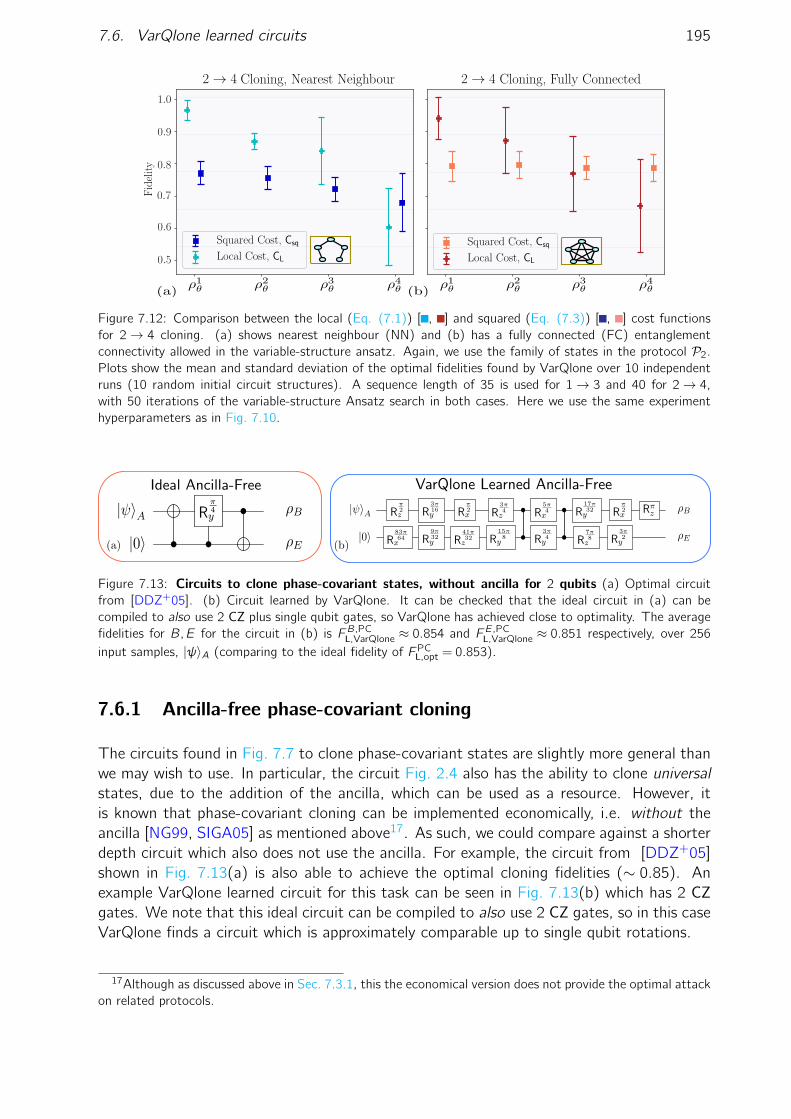
7.6. VarQlone learned circuits 195
Figure 7.12: Comparison between the local (Eq. (7.1)) [ , ] and squared (Eq. (7.3)) [ , ] cost functionsfor 2→ 4 cloning. (a) shows nearest neighbour (NN) and (b) has a fully connected (FC) entanglementconnectivity allowed in the variable-structure ansatz. Again, we use the family of states in the protocol P2.Plots show the mean and standard deviation of the optimal fidelities found by VarQlone over 10 independentruns (10 random initial circuit structures). A sequence length of 35 is used for 1→ 3 and 40 for 2→ 4,with 50 iterations of the variable-structure Ansatz search in both cases. Here we use the same experimenthyperparameters as in Fig. 7.10.
Figure 7.13: Circuits to clone phase-covariant states, without ancilla for 2 qubits (a) Optimal circuitfrom [DDZ+05]. (b) Circuit learned by VarQlone. It can be checked that the ideal circuit in (a) can becompiled to also use 2 CZ plus single qubit gates, so VarQlone has achieved close to optimality. The averagefidelities for B,E for the circuit in (b) is FB,PC
L,VarQlone ≈ 0.854 and FE,PCL,VarQlone ≈ 0.851 respectively, over 256
input samples, |ψ〉A (comparing to the ideal fidelity of FPCL,opt = 0.853).
7.6.1 Ancilla-free phase-covariant cloning
The circuits found in Fig. 7.7 to clone phase-covariant states are slightly more general thanwe may wish to use. In particular, the circuit Fig. 2.4 also has the ability to clone universalstates, due to the addition of the ancilla, which can be used as a resource. However, itis known that phase-covariant cloning can be implemented economically, i.e. without theancilla [NG99, SIGA05] as mentioned above17. As such, we could compare against a shorterdepth circuit which also does not use the ancilla. For example, the circuit from [DDZ+05]shown in Fig. 7.13(a) is also able to achieve the optimal cloning fidelities (∼ 0.85). Anexample VarQlone learned circuit for this task can be seen in Fig. 7.13(b) which has 2 CZgates. We note that this ideal circuit can be compiled to also use 2 CZ gates, so in this caseVarQlone finds a circuit which is approximately comparable up to single qubit rotations.
17Although as discussed above in Sec. 7.3.1, this the economical version does not provide the optimal attackon related protocols.

196 7. Practical quantum cryptanalysis by variational quantum cloning
Figure 7.14: Circuit learned by VarQlone in to clone states, |φ0〉, |φ1〉, with an overlap s = cos(π/9) inthe protocol, P1. For example, ρA is the clone sent back to Alice, while ρB is kept by Bob.
Figure 7.15: Circuits learned by VarQlone to clone states from the protocol, P2 for (a) 1→ 2, (b) 1→ 3
and (c) 2→ 4 cloning. These specific circuits produce the fidelities in Fig. 7.9(b) for 1→ 2, (using the localcost function), and in Fig. 7.10 for 1→ 3 and 2→ 4 (using the squared cost function). We allow an ancillafor all circuits, and ρk indicates the qubit which will be the kth output clone.
7.6.2 State-dependent cloning circuits
Fig. 7.14 shows the circuit used to achieve the fidelities in the attack on P1. In training, westill allow an ancilla to aid the cloning, but the example in Fig. 7.14 did not make use of it(in other words, VarQlone only applied gates which resolved to the identity on the ancilla),so we remove it to improve hardware performance. This repeats the behaviour seen for thecircuits learned in phase-covariant cloning. We mention again, that some of the learnedcircuits did make use of the ancilla with similar performance.
Fig. 7.15 shows the circuits learned by VarQlone and approximately clone all four statesin Eq. (7.76) in the protocol, P2, for 1→ 2,1→ 3 and 2→ 4 cloning. These are the specificcircuits used to produce the fidelities in Fig. 7.9(b) and Fig. 7.10.

7.7. Discussion and conclusions 197
7.7 Discussion and conclusions
We have now concluded the discussion of our third and final application for near-term quan-tum computers; the use of quantum machine learning in quantum information and quantumcryptography. We saw how quantum cloning is one of the most important ingredients notjust as a tool in quantum cryptanalysis, but also with roots in foundational questions ofquantum mechanics. However, given the amount of attention this field has received, afundamental question remained elusive: how do we construct efficient, flexible, and noise-tolerant circuits to actually perform approximate or probabilistic cloning? We demonstratedhow VarQlone provided a novel toolkit to such an exercise. We further believe that VarQloneis unique among variational/quantum machine learning algorithms for a number of reasons.The first, and most obvious reason for this is that it bridges the fields of quantum ma-chine learning and quantum cryptography in an interesting manner. We demonstrated howVarQlone brings into view a whole new domain of performing realistic implementation ofattacks on quantum cryptographic systems. Secondly, since it is an example using quantumdata directly, there is no obvious method of dequantisation, or indeed no obvious argu-ment why dequantisation would even make sense in such a context. Finally, unlike manyother variational algorithms, which aim to mimic performance of fault-tolerant algorithmsin asymptotic scaling regimes, it is useful in both the small scale, and the large scale. Theformer is more obvious; we have already demonstrated example use cases ion cryptography.At the larger scale, one could imagine studying connections to quantum state estimation,or simply the question of cloning by itself.
In future work, one of the most exciting possible directions is in actually using VarQloneto aid the attack of a quantum protocol in a physical experiment. Other directions ofstudy include improving the robustness and performance of VarQlone. One could utilisenoise tolerant methods for quantum architecture search, or incorporating error mitigationmethods. The latter presents an interesting question in itself, since many error mitigationmethods aim to correct expectation values of computations by classical post-processing. Itis not obvious how such techniques may be useful when the desired output is not classical.


8
Conclusion
This Thesis began with the goal of finding, and developing, applications and models for near-term quantum computers. Focusing on problems and techniques from quantum machinelearning, we aimed to attach theoretical rigour, where possible, to an experimental plug-and-play mindset in the development of such applications. We focused on a particular primitivefrom modern quantum machine learning; the variational quantum algorithm (VQA) equippedwith the parameterised quantum circuit (PQC). Let us now conclude the Thesis by brieflysummarising the contributions of each chapter, before discussing a more general outlookand future directions.
As a reminder, this Thesis was structured in accordance with the increasing complexityof the data available to each application.
We began in Chapter 5 with labelled vectors as data and focused on the use of a PQCin supervised learning for the problem of classification. In order to build such models tobe implementable across multiple types of near-term quantum hardware, it is importantto build them in a robust manner, to account for the inevitable quantum noise which willplague them for at least the next several years. We did this by focusing attention on themeans of encoding data into the PQC for subsequent classification. We provided severaldefinitions for ‘robust’ data encodings, and we proved that such encodings must alwaysexist, for a given noise channel. We also studied the design of the PQC outside of the dataencoding, and found that by incorporating simple alternative design principles, the modelcould be naturally robust. However, we noted that this robustness came at a price; namelyin the expressiveness or learnability of the model. Finally, we performed several numericalexperiments demonstrating that an ‘optimal’ classifier for near-term devices involves a trade-off between robustness and learnability.
Next, in Chapter 6 we turned to the more complicated unsupervised learning problem ofgenerative modelling. Here, the data becomes probability distributions and sample access tothem. To attack this problem, we turn to a PQC in the form of a Born machine, an implicitgenerative model suitable for near-term devices. We began by discussing the possibility ofa (provable) quantum advantage in generative modelling and natural reasons why the Bornmachine may demonstrate such a thing. We then developed new gradient-based trainingmethods for the Born machine by changing the cost function used. Finally, we performedan extensive numerical and experimental study for the Born machine with three differentdatasets. Of particular interest, was that one of these datasets originated with a quantumprocess, which one of the others was relevant to a real world use case in finances. In thislatter example, we also performed a comparison to a comparable classical generative model,
199

200 8. Conclusion
the restricted Boltzmann machine, and found that the quantum model could outperform itsclassical counterpart (a numerical quantum advantage). We also surprisingly found someevidence that entanglement may be partially responsible for such an advantage, by addingcorrelations which are not classically accessible.
Finally, in Chapter 7 we changed course slightly away from ‘machine learning’ problems,into the domain of quantum foundations. However, we still used very similar ML tools in thestudy of quantum cloning. Here, we designed a variational quantum algorithm (VarQlone)to learn to approximately clone quantum states. For the algorithm, we provided cost func-tions with faithfulness guarantees, derived suitable gradients for gradient-based training,and incorporated quantum architecture search to find high quality cloning circuits. In thischapter, we also made an interesting bridge between quantum machine learning and quan-tum cryptography by demonstrating how QML methods could be used as a subroutine intools for the cryptanalysis of quantum protocols. Specifically for this latter use case, wefocused on the common examples of quantum key distribution, and quantum coin flipping.We illustrated how VarQlone could be used to find novel attacks on such protocols, whichcould subsequently be employed to improve the protocols.
Returning to an abridged version of the question posed in the Introduction (“How canwe use the quantum computers we have now . . . ”), it is clear that there are a multitudeof potential applications for such devices. Whether any of these will prove to be the ‘killerapplication’, only time (and bigger quantum computers) will tell. This breakthrough maycome from a dedicated research team in a multinational conglomerate, or even from a lone‘quantum hacker’. Both of these are now possible due to the abundance of resources andlearning material. Regardless, the sheer scope of possibility is one of the main reasons whythere is excitement and hype surrounding the field. While such excitement is extremelybeneficial for a number of reasons, we must also be careful to temper unfounded claims ofquantum computers revolutionising all aspects of science and technology. Throughout thisthesis, I hope I have been able to provide a balanced view.
My PhD has been fortunately situated in the era of the first commercially availablequantum computers. As such, it was perfectly positioned in the QML transition period totake advantage of these computers. With this in mind, I would summarise my experienceof performing research in quantum machine learning as the perfectly epitomised quote bythe Doctor: “ . . . It’s a bit dodgy, this process. You never know what you’re going to endup with.”, which applies equally well to both its parent fields.

Appendix A
Proofs and derivations
A.1 Proofs for Chapter 5
A.1.1 Proofs of Theorem 9 and Theorem 10
Here we give the proofs of the above two Theorems, which broadly have the same structure.
Theorem 9. If E is any noise channel which factorises into a single qubit channel,and a multiqubit channel as follows:
E(ρ) = Ec(ρcx)⊗Ec(ρcx)
where WLOG Ec acts only on the classification qubit (ρcx = Trc(ρx)) after encodingand unitary evolution, and Ec acts on all other qubits arbitrarily, (ρcx = Trc(ρx)).Further assume the state meets the robust classification requirements for the singlequbit error channel Ec . Then the classifier will be robust to E .
Proof. The correct classification again depends on the classification qubit measurementprobabilities: Tr(|0〉〈0|c ⊗1⊗n−1ρx),Tr(|1〉〈1|c ⊗1⊗n−1ρx). If ρx is robust to the singlequbit error channel Ec , this means
Tr(Πc0ρx)> 1/2 =⇒ Tr(Πc0Ec(ρx))> 1/2
Tr(Πc1ρx)< 1/2 =⇒ Tr(Πc1Ec(ρx))< 1/2
Then WLOG, assume the point x classified as y(ρx) = 0 before the noise, then:
Tr (Πc0E(ρx)) = Tr(
Πc0[Ec(ρcx ⊗Ec(ρcx)
])= Trc
(Ec(ρcx)
)Trc (|0〉〈0 |Ec(ρcx))
= Tr (|0〉〈0 |Ec(ρcx))> 1/2
201

202 Appendix A. Proofs and derivations
Theorem 10. Let Emeasp define measurement noise acting on the classification qubit
and consider a quantum classifier on data from the set X . Then, for any encodingE : X → S2, we have complete robustness
R(Emeasp ,E, y) = X
if the measurement assignment probabilities satisfy p00 > p01,p11 > p10.
Proof. We can write the measurement noise channel acting on the POVM elements as:
Emeasp (Πc0⊗1⊗n−1) = (p00|0〉〈0 |+p01|1〉〈1 |)⊗1⊗n−1
Again, if we had correct classification before the noise, Tr(|0〉〈0|ρx)> 1/2, then:
Tr[Emeasp (Πc0⊗1⊗n−1)ρx ] = Tr[(p00|0〉〈0 |+p01|1〉〈1 |⊗1⊗n−1)ρx ]
= p00Tr[(|0〉〈0|⊗1⊗n−1)ρx ] +p01Tr[(|1〉〈1 |⊗1⊗n−1)ρx ]
= p00Tr[(|0〉〈0|⊗1⊗n−1)ρx ] +p01(1−Tr[(|0〉〈0|⊗1⊗n−1)ρx ])
= (p00−p01)Tr[(|0〉〈0 |⊗1⊗n−1)ρx ] +p01
> (p00−p01)1
2+p01 =
1
2(p00 +p01) =
1
2
A.1.2 Proof of Theorem 14
Here we prove the above Theorem for a bound on the size of the robust set.
Theorem 14. Consider a quantum classifier using the mixed state encoding Eq.(5.63) and indicator cost function Eq. (5.64). Assuming that a noise channel Eacts only on the encoded feature vectors ρx i (and not the encoded labels |yi〉〈yi |),then
|R(E ,E, y)|>M[
1−√
1−F (E(σ), σ)]
(A.1)
where F is the fidelity between quantum states, Eq. (2.69).
This Theorem is useful since, if one has an expression for the output fidelity of a quantumcircuit after a noise channel is applied, one can directly determine a bound on how theclassification results will be affected. In order to prove it, we relate the difference betweenthe noisy cost and the noiseless cost to the size of the robust set.
Proof. Let the indicator cost Eq. (5.64) of the noisy classifier be CE and the noiselessclassifier be C. Define
∆E C := |CE−C | (A.2)
to be the magnitude of the difference between noisy and noiseless costs. Due to ourchoice of cost function Eq. (5.64), we can relate ∆E C to the δ-robustness of the model inDefinition 33 as follows.

A.1. Proofs for Chapter 5 203
First, it is easy to see that the quantity 1−∆E C is the the fraction δ of robust points Eq.(5.20) so that:
|R(E ,E, y)|=M (1−∆E C) (A.3)
Now, the PQC acts only on the “data subsystem” of the mixed state encoding Eq. (5.63)so that the evolved state before measurement is:
σ =1
M
M
∑i=1
ρx i ⊗|yi〉〈yi | (A.4)
By assumption, the channel E leaves the “label subsystem” |yi〉〈yi | invariant so that:
E(σ) =1
M
M
∑i=i
E(ρx i)⊗|yi〉〈yi |
Now, a related cost C′ can be evaluated by measuring the expectation of:
D := 1⊗n−1⊗Zc ⊗Zl
where c and l denote classification and label qubits, respectively [CWV+19]. That is, thenoiseless cost is given by
C′ = Tr(Dσ)
and the noisy cost is given by
C′E = Tr(DE(σ)).
Now, it is easy to see that 06 ∆E C′ 6 2. When all points are robust, ∆E C
′ = 0, and whena single point goes from robust to not robust, ∆E C
′ increases by at most 2/M. As such,we can write down a corresponding inequality for the cost, C′, as in Eq. (A.3) so that
|R(E ,E, y)|>M(
1−∆E C
′
2
). (A.5)
The difference in cost Eq. (A.2) due to noise is thus
∆E C′ :=
∣∣C′E−C′∣∣= |Tr[D(E(σ)− σ)]|
6 ||D||∞||E(σ)− σ||1
6 2√
1−F (E(σ), σ). (A.6)
The third line in this derivation follows from Hölders inequality and the last line from theFuchs-van de Graaf inequality [GCP+20, FG99]. We also used the fact that ||D||∞ :=
maxj |λj(D)|= 1.Substituting the inequality Eq. (A.5) in Eq. (A.6) completes the proof.

204 Appendix A. Proofs and derivations
A.2 Proofs for Chapter 7
A.2.1 Proof of gradients for VarQlone
We do this explicitly for the squared local cost, Eq. (7.3), and for brevity neglect thegradient derivations for the others, since they are simpler and follow analogously. For thiscost function we have the gradient with respect to a parameter, θl as:
∂Csq(θ)
∂θl= 2E
[∑i<j
(F iL−FjL)(Fi ,l+π
2L −F i ,l−
π2
L −F j,l+π2
L +Fj,l−π2L
)−∑
i
(1−F iL)(Fi ,l+π
2L −F i ,l−
π2
L )
](A.7)
where F j,l±π/2L (θ) denotes the fidelity of a particular state, |ψ〉, with j th reduced state of
the VarQlone circuit which has the l th parameter shifted by ±π/2. We suppress the θdependence in the above.
Proof. We begin as before, by taking the derivative of Eq. (7.3) with respect to a singleparameter, θl :
∂Csq(θ)
∂θl= 2 E
|ψ〉∈S
[N
∑i=1
(1−F iL(θ))
[−∂F iL(θ)
∂θl
]
+N
∑i<j
(F iL(θ)−F jL(θ))
[∂F iL(θ)
∂θl−∂F jL(θ)
∂θl
]]We can rewrite the expression for the fidelity of the j th clone as:
F jL(θ) = 〈ψ|ρj(θ)|ψ〉= Tr[|ψ〉〈ψ|ρj
]= Trj
[|ψ〉〈ψ|Trj
(U(θ)ρinitU(θ)†
)](A.8)
Using the linearity of the trace, the derivative of the fidelities with respect to the pa-rameters, θl , can be computed:
∂F jL(θ)
∂θl= Trj
[|ψ〉〈ψ|Trj
(∂U(θ)ρinitU(θ)†
∂θl
)](A.9)
Now plugging in the parameter shift rule:
∂U(θ)ρinitU(θ)†
∂θl= U l+
π2 (θ)ρinit(U(θ)l+
π2 )†−U l−
π2 (θ)ρinit(U(θ)l−
π2 )† (A.10)
Where the notation, U l±π2 , indicates the l th parameter has been shifted by ±π2 , i.e. U
l±π2 :=
U(θd) . . .U(θl ± π/2) . . .U(θ1). Now:
∂F jL(θ)
∂θl= Trj
[|ψ〉〈ψ|Trj
(U l+
π2 (θ)ρinit(U(θ)l+
π2 )†)]
−Trj
[|ψ〉〈ψ|Trj
(U l−
π2 (θ)ρinit(U(θ)l−
π2 )†)]
=⇒∂F jL(θ)
∂θl= Tr
[|ψ〉〈ψ|ρl+
π2
j (θ)]−Tr
[|ψ〉〈ψ|ρl−
π2
j (θ)]
(A.11)
= F(j,l+π
2 )
L (θ)−F (j,l−π2 )
L (θ) (A.12)

A.2. Proofs for Chapter 7 205
where we define F(l±π2 )
j (θ) := 〈ψ|ρl±π2
j (θ)|ψ〉 the fidelity of the j th clone, when preparedusing a unitary whose l th parameter is shifted by ±π2 , with respect to a target input state,|ψ〉.
Plugging Eq. (A.12) into Eq. (A.10), we recover the expression in Eq. (A.7).
A.2.2 Proof of Theorem 19
Theorem 19. The squared cost function as defined Eq. (7.15), is ε-weakly faithfulwith respect to the Bures angle distance measure dBA. In other words, if we have:
Csq(θ)−Coptsq 6 ε (A.13)
where Coptsq := (Fi(θ)−Fj(θ))2 = N(1−Fopt)2 is the optimal cost, then the following
fact holds:
dBA(ρψ,jθ ,ρψ,jopt)6N ε
2(1−Fopt)sin(Fopt):= f1(ε), ∀|ψ〉 ∈ S,∀j ∈ [N] (A.14)
Proof. To prove Theorem 19, we revisit and rewrite the Bures angle from Eq. (2.70)as [NC10]:
dBA(ρ,σ) = arccos√F (ρ,σ) = arccos〈φ|τ〉 (A.15)
where |φ〉 and |τ〉 are the purifications1 of ρ and σ respectively which maximise the overlap.We note that dBA(ρ,σ) lies between [0,π/2], with dBA(ρ,σ) = π/2 corresponding to ρ= σ.Since this distance is a metric, it obeys the triangle inequality (Definition 9), i.e., for anythree states ρ,σ and δ,
dBA(ρ,σ)6 dBA(ρ,δ) +dBA(σ,δ) (A.16)
Rewriting the result of Lemma 2 in terms of fidelity for each |ψ〉 ∈ S and correspondinglyin terms of Bures angle using Eq. (A.15) is,
F (ρψ,jopt, |ψ〉)−F (ρψ,jθ , |ψ〉)6 ε′
=⇒ cos2(dBA(ρψ,jopt, |ψ〉))−cos2(dBA(ρψ,jθ , |ψ〉))6 ε′(A.17)
where ε′ = N ε2(1−Fopt) . Let us denote D
ψ± = dBA(ρψ,jopt, |ψ〉)±dBA(ρψ,jθ , |ψ〉) This inequality in
Eq. (A.17) can be further rewritten as,
cos(dBA(ρψ,jopt, |ψ〉))−cos(dBA(ρψ,jθ , |ψ〉))6ε′
cos(dBA(ρψ,jopt, |ψ〉)) + cos(dBA(ρψ,jθ , |ψ〉))
cos(dBA(ρψ,jopt, |ψ〉))−cos(dBA(ρψ,jθ , |ψ〉))/ε′
2cos(dBA(ρψ,jopt, |ψ〉))
2sin
(Dψ+
2
)sin
(dψ−2
)6
ε′
2cos(dBA(ρψ,jopt, |ψ〉))
=⇒ dψ− 6ε′
sin(dBA(ρψ,jopt, |ψ〉))=
N ε2(1−Fopt)sin(Fopt)
(A.18)
1A purification of a mixed state, ρ ∈ HA, is a pure state, |ψ〉, in a larger Hilbert space (HA⊗HB) suchthat tracing out B leaves the original state, ρ, ρ= TrB(|ψ〉〈ψ |).

206 Appendix A. Proofs and derivations
In the above, we use the approximations that as ε→ 0, dBA(ρψ,jopt, |ψ〉)≈ dBA(ρψ,jθ , |ψ〉) andthe trigonometric identities cos(x − y) = 2sin
(x+y
2
)sin(x−y
2
), and sin2x = 2sinx cosx .
Now, using the triangle inequality on the states ρψ,jopt,ρψ,jθ , |ψ〉, we have:
dBA(ρψ,jθ , |ψ〉)6 dBA(ρψ,jopt, |ψ〉) +dBA(ρψ,jθ ,ρψ,jopt) (A.19)
Combining the above inequality and Eq. (A.18) completes the proof:
dBA(ρψ,jθ ,ρψ,jopt)6N ε
2(1−Fopt)sin(Fopt), ∀|ψ〉 ∈ S (A.20)
A.2.3 Proof of Theorem 20
Here we give the proof of Theorem 20. We begin by repeating the Theorem:
Theorem 20. The squared cost function, Eq. (7.15), is ε-weakly faithful with respectto the trace distance dTr.
dTr(ρψ,jopt,ρ
ψ,jθ )6 g1(ε), ∀j ∈ [N] (A.21)
where:
g1(ε)≈1
2
√4Fopt(1−Fopt) +ε
N (1−2Fopt)
2(1−Fopt)(A.22)
Proof. Firstly, we note that Fopt = 〈ψ|ρψ,jopt|ψ〉 is the same value for all input states |ψ〉 ∈ S.We apply the change of basis from |ψ〉 → |0〉 by applying the unitary V |ψ〉= |0〉. Then theeffective change on the state ρψ,jopt to have a fidelity Fopt with the state |0〉 is, ρψ,jopt→ V ρψ,joptV
†,written as:
V ρψ,joptV† =
(Fopt a∗
a 1−Fopt
)(A.23)
where we use the usual properties of a density matrix and a ∈C. The upper bound conditionin Eq. (7.19) states that:
〈ψ|ρψ,jopt−ρψ,jθ |ψ〉= 〈0|V (ρψ,jopt−ρ
ψ,jθ )V †|0〉=
N ε2(1−Fopt)
=: ε′
V has the following effect on ρψ,jθ :
V ρψ,jθ V † =
(Fopt +ε′ b∗
b 1− (Fopt +ε′)
)(A.24)
for some b ∈ C. The condition that V ρψ,joptV†,V ρψ,jθ V † > 0 i.e. they are positive, implies
that,
|a|2 6 Fopt(1−Fopt) =: r2Fopt
, |b|2 6 (Fopt +ε′)(1− [Fopt +ε′]) =: rFopt+ε′ (A.25)
Using the relationship between the trace distance and the positive eigenvalue of the dif-ference between the states, we consider the eigenvalues of V ρψ,joptV
†− V ρψ,jθ V †. The two

A.2. Proofs for Chapter 7 207
eigenvalues of this matrix is λ± =±√ε′2 + |a−b|2. From this, the trace distance between
the two states is,
dTr(V ρψ,joptV
†,V ρψ,jθ V †) =1
2
∣∣∣∣∣∣V ρψ,joptV†−V ρψ,jθ V †
∣∣∣∣∣∣=1
2|λ+|=
1
2
√ε′2 + |a−b|2 (A.26)
We note that the trace distance is unitary invariant. Thus,
dTr(ρψ,jopt,ρ
ψ,jθ ) = dTr(V ρ
ψ,joptV
†,V ρψ,jθ V †)
=1
2
√ε′2 + |a−b|2
61
2
√ε′2 + (rFopt + rFopt+ε′)2
≈1
2
√4Fopt(1−Fopt) +ε′(1−2Fopt)
=1
2
√4Fopt(1−Fopt) +ε
N (1−2Fopt)
2(1−Fopt)
(A.27)
where we have used the inequality |a−b|2 6 ||a|+ |b||2 for all a,b ∈ C.
A.2.4 Proof of Theorem 26
Here we give the proof of Theorem 26 which is repeated below:
Theorem 26. For the general case of M→N cloning, the global cost function CG(θ)
and the local cost function CL(θ) satisfy the inequality,
CL(θ)6 CG(θ)6 N ·CL(θ) (A.28)
Proof. We first prove the first part of the inequality,
CG(θ)−CL(θ) =1
N
∫STr((OψG−OψL )ρψθ )dψ
=1
NN
∫STr
((N
∑j=1
(|ψ〉〈ψ |j ⊗1j −|ψ〉〈ψ |1⊗·· · |ψ〉〈ψ |N
))ρψθ
)> 0
=⇒ CG(θ)> CL(θ)
(A.29)
where OψL is defined in Eq. (7.2), and the inequality in the second line holds because
N
∑j=1
(|ψ〉〈ψ |j ⊗1j −|ψ〉〈ψ |1⊗·· · |ψ〉〈ψ |N
)=
N
∑j=1
|ψ〉〈ψ |j ⊗ (1j −|ψ〉〈ψ |j)> 0, ∀|ψ〉 ∈ S (A.30)

208 Appendix A. Proofs and derivations
For the second part of the inequality, we consider the operator NOψL −OψG,
NOψL −OψG = (N−1)1−N
∑j=1
(|ψ〉〈ψ |j ⊗1j
)+ |ψ〉〈ψ |1⊗·· ·⊗ |ψ〉〈ψ |N
=N−1
∑j=1
(1j ⊗1j −|ψ〉〈ψ |j ⊗1j
)−|ψ〉〈ψ |N⊗1N + |ψ〉〈ψ |1⊗·· ·⊗ |ψ〉〈ψ |N
=N−1
∑j=1
((1−|ψ〉〈ψ |)j ⊗1j
)−N−1⊗j=1
(1−|ψ〉〈ψ |)j ⊗|ψ〉〈ψ |N
= (1−|ψ〉〈ψ |)1⊗
(11−
N−1⊗j=2
(1−|ψ〉〈ψ |j)⊗|ψ〉〈ψ |N
)
+N−1
∑j=2
((1−|ψ〉〈ψ |)j)⊗1j
)> 0
(A.31)
where the second last line is positive because each individual operator is positive for all|ψ〉 ∈ S.
A.2.5 Proof of Theorem 30
Here we give the proof of faithfulness for the asymmetric cost function, Theorem 30.
Theorem 30. The asymmetric cost function, Eq. (7.55), is ε-weakly faithful withrespect to dBA:
CL,asym(θ)−CoptL,asym 6 ε (A.32)
where CoptL,asym = 0. then the following fact holds for Bob and Eve’s reduced states::
dBA(ρψ,Bθ ,ρψ,Bopt )6
√N ε
sin(1−p2/2), dBA(ρψ,Eθ ,ρψ,Eopt )6
√N ε
sin(1−q2/2)(A.33)
Furthermore, we also have the following trace distance bounds:
dTr(ρψ,B,ρψ,Bθ )6
1
2
√p2(2−p2)−
√N ε(1−p2), (A.34)
dTr(ρψ,E,ρψ,Eθ )6
1
2
√q2(2−q2)−
√N ε(1−q2) (A.35)
Proof. Firstly, we derive a similar result to Lemma 2 and Lemma 3. By expanding the term|CL,asym(θ)−CL,opt | in terms of the corresponding output states, we obtain,
|CL,asym(θ)−CL,opt |=∣∣∣∣ 1
N
∫S
((F p,BL −FBL (θ))2 + (F p,EL −FEL (θ))2
)dψ
∣∣∣∣=
1
N
∫S
[(Tr[(ρψ,B−ρψ,Bθ )|ψ〉〈ψ|]
)2+(Tr[(ρψ,E−ρψ,Eθ )|ψ〉〈ψ|]
)2]dψ
(A.36)

A.2. Proofs for Chapter 7 209
Using the inequality Eq. (A.32) and Eq. (A.36), we get,
1
N
∫S
(Tr[(ρψ,jopt−ρ
ψ,jθ )|ψ〉〈ψ|]
)2dψ 6 ε =⇒ Tr[(ρψ,jopt−ρ
jθ)|ψ〉〈ψ|]6
√N ε (A.37)
where j ∈ B,E.Next, to derive Eq. (A.33) we rewrite the Eq. (A.37) in terms of the Bures angle:
F (ρψ,jopt, |ψ〉)−F (ρψ,jθ , |ψ〉)6√N ε
=⇒ cos2(dBA(ρψ,jopt, |ψ〉))−cos2(dBA(ρψ,jθ , |ψ〉))6√N ε
(A.38)
Following the derivations in the previous sections, we have:
dBA(ρψ,jθ ,ρψ,jopt)6
√N ε
sin(F r,jL ), ∀|ψ〉 ∈ S (A.39)
where F r,jL is the optimal cloning fidelity corresponding to j ∈ B,E with r ∈ p,q. Finally,plugging in the optimal asymmetric fidelities, F p,BL = 1− p2/2, and similarly for F q,EL wearrive at:
dBA(ρψ,Bθ ,ρψ,Bopt )6
√N ε
sin(1−p2/2), dBA(ρψ,Eθ ,ρψ,Eopt )6
√N ε
sin(1−q2/2)(A.40)
Finally, to prove Eq. (A.34), we follow the trace distance derivation bounds as in previoussections and obtain:
dTr(ρψ,j ,ρψ,jθ )6
1
2
√4F r,jL (1−F r,jL ) +
√N ε(1−2F r,jL ) (A.41)
Again, plugging in the optimal fidelities for Bob and Eve completes the proof.
A.2.6 Proof of Theorem 31
Here we prove Theorem 31 in the main text.
Theorem 31 (Sample complexity of VarQlone). The number of samples L×K re-quired to estimate the VarQlone cost function C(θ) up to ε′-additive error with asuccess probability δ is:
L×K =O(
1
ε′2log
2
δ
)(A.42)
where K is the number of distinct states |ψ〉 sampled uniformly at random from thedistribution S, and L is the number of copies of each input state.
Proof. We provide the proof for the cost function CG(θ). However, this proof extends in astraightforward manner to other cost functions. As a reminder, the global cost function isdefined as,
CψG(θ) = 1−〈φ|ρψθ |φ〉 =⇒ CG(θ) = 1−1
N
∫S〈φ|ρψθ |φ〉dψ (A.43)

210 Appendix A. Proofs and derivations
The estimation of CψG(θ) requires the computation of the overlap 〈φ|ρψθ |φ〉. Let us denote|φ〉 := |ψ〉⊗N as an N-fold tensor product of the input state.
This test inputs the states |φ〉 and ρψθ with an additional ancilla qubit |0〉, and measuresthe ancilla in the end in the computational basis. The probability of obtaining an outcome‘1’ in the measurement is (recall 1−Pr[|anc〉= |0〉] from Eq. (2.76)):
Pr[|anc〉= |1〉] = pψ =1
2(1−〈φ|ρψθ |φ〉) (A.44)
From this, we see that CψG(θ) = 2pψ. To estimate this cost function value, we run theSWAP test L times and estimate the averaged number of ‘1’ outcomes. Let us the definethe estimator for cost function with L samples to be,
Cψ
G,avg(θ) =1
L
L
∑i=1
Cψ
G,i(θ) (A.45)
where Cψ
G,i(θ) is equal to 2 if the SWAP test outcome at the i-th run is ‘1’ and is 0 otherwise.
From this we can see that the expected value of Cψ
G,avg(θ) is,
E[Cψ
G,avg(θ)]
= CψG(θ) = 2pψ (A.46)
Now consider K different states |ψ1〉, · · · |ψK〉 are chosen uniformly at random from thedistribution S. The average value of the cost over K is:
CG,avg(θ) =1
K
K
∑j=1
CψjG,avg(θ) =
1
LK
K
∑j=1
L
∑i=1
CψjG,i(θ) (A.47)
with,
E[CG,avg(θ)
]=
1
K
K
∑j=1
1
N
∫SCψ
G,avg(θ)dψ = CG(θ) (A.48)
Using Höeffding’s inequality [Hoe63], we obtain a probabilistic bound on |CG,avg(θ)−CG(θ)|,
Pr[|CG,avg(θ)−CG(θ)|> ε′
]6 2e−2KLε′2 (A.49)
Now, setting 2e−2KLε′2 = δ and solving for L×K gives:
L×K =O(
1
ε′2log
2
δ
)(A.50)
A.2.7 Proof of Theorem 34
Here we prove Theorem 34. We repeat the Theorem first:
Theorem 34 (Ideal cloning attack (II) bias on P2 in scenario 1.).Using a cloning attack on the protocol, P2, (in attack model II with 4 states) Bobcan achieve a bias:
εIIP2,ideal = 0.25 (A.51)

A.2. Proofs for Chapter 7 211
Proof. Considering the 4 states to be in the X−Z plane of the Bloch sphere, the densitymatrices of each state can be represented as:
ρi j =1
2(1+mi jx X+mi jz Z) (A.52)
where X and Z are Pauli matrices and each mi j is a three dimensional vector given by:
m00 := [sin(2φ), 0, cos(2φ)]
m01 := [−sin(2φ), 0, −cos(2φ)]
m10 := [−sin(2φ), 0, cos(2φ)]
m11 := [sin(2φ), 0, −cos(2φ)]
(A.53)
After the cloning (in the ideal case), the density matrix of each clone will become:
ρci j =1
2(1+ηxm
i jx X+ηzm
i jz Z) (A.54)
where ηx and ηz are the shrinking factors in each direction given as follows:
ηx = sin2(2φ)
√1
sin4(2φ) + cos4(2φ), ηz = cos2(2φ)
√1
sin4(2φ) + cos4(2φ)(A.55)
For the states used in P2, we have φ = π8 and hence ηx = ηz := η = 1√
2. Again, we can
return to the discrimination probability between the two ensembles encoding a= 0 and a= 1
in Eq. (7.84). Here, we have (let us define ρc to be the output clone that Bob chooses touse (c ∈ 1,2):
P opt,IIdisc,P2
=1
2+
1
4
∣∣∣∣ρ(a=0)−ρ(a=1)
∣∣∣∣Tr
=1
2+
1
4
∣∣∣∣∣∣∣∣12 [(ρc00−ρc11) + (ρc10−ρc01)]
∣∣∣∣∣∣∣∣Tr
=1
2+
1
4
∣∣∣∣∣∣η4
(mx00−mx11 +mx10−mx01)X+ (mz00−mz11 +mz10−mz01)Z∣∣∣∣∣∣Tr
=1
2+η cos(2φ)
4||Z||Tr
=1
2+η cos(2φ)
2=
3
4
Computing the bias in the same way as done previously completes the proof.


Bibliography
[AAB+19] Frank Arute, Kunal Arya, Ryan Babbush, Dave Bacon, Joseph C. Bardin,Rami Barends, Rupak Biswas, Sergio Boixo, Fernando G. S. L. Brandao,David A. Buell, Brian Burkett, Yu Chen, Zijun Chen, Ben Chiaro, RobertoCollins, William Courtney, Andrew Dunsworth, Edward Farhi, Brooks Foxen,Austin Fowler, Craig Gidney, Marissa Giustina, Rob Graff, Keith Guerin,Steve Habegger, Matthew P. Harrigan, Michael J. Hartmann, Alan Ho,Markus Hoffmann, Trent Huang, Travis S. Humble, Sergei V. Isakov, EvanJeffrey, Zhang Jiang, Dvir Kafri, Kostyantyn Kechedzhi, Julian Kelly, Paul V.Klimov, Sergey Knysh, Alexander Korotkov, Fedor Kostritsa, David Land-huis, Mike Lindmark, Erik Lucero, Dmitry Lyakh, Salvatore Mandrà, Jar-rod R. McClean, Matthew McEwen, Anthony Megrant, Xiao Mi, KristelMichielsen, Masoud Mohseni, Josh Mutus, Ofer Naaman, Matthew Neeley,Charles Neill, Murphy Yuezhen Niu, Eric Ostby, Andre Petukhov, John C.Platt, Chris Quintana, Eleanor G. Rieffel, Pedram Roushan, Nicholas C. Ru-bin, Daniel Sank, Kevin J. Satzinger, Vadim Smelyanskiy, Kevin J. Sung,Matthew D. Trevithick, Amit Vainsencher, Benjamin Villalonga, TheodoreWhite, Z. Jamie Yao, Ping Yeh, Adam Zalcman, Hartmut Neven, andJohn M. Martinis. Quantum supremacy using a programmable supercon-ducting processor. Nature, 574(7779):505–510, October 2019. Nature,574(7779):505–510. 3, 19, 67
[Aar09] Scott Aaronson. Quantum Copy-Protection and Quantum Money. In Pro-ceedings of the 2009 24th Annual IEEE Conference on Computational Com-plexity, CCC ’09, pages 229–242, USA, July 2009. IEEE Computer Society.CCC ’09, pages 229–242. 154
[Aar15] Scott Aaronson. Read the fine print. Nature Physics, 11(4):291–293, April2015. Nature Physics, 11(4):291–293. 55
[AAR+18] Mohammad H. Amin, Evgeny Andriyash, Jason Rolfe, Bohdan Kulchyt-skyy, and Roger Melko. Quantum Boltzmann Machine. Physical ReviewX, 8(2):21050, May 2018. PRX, 8(2):21050. 54, 133
[ABB+21] J. M. Arrazola, V. Bergholm, K. Brádler, T. R. Bromley, M. J. Collins,I. Dhand, A. Fumagalli, T. Gerrits, A. Goussev, L. G. Helt, J. Hundal,T. Isacsson, R. B. Israel, J. Izaac, S. Jahangiri, R. Janik, N. Killoran, S. P.Kumar, J. Lavoie, A. E. Lita, D. H. Mahler, M. Menotti, B. Morrison, S. W.Nam, L. Neuhaus, H. Y. Qi, N. Quesada, A. Repingon, K. K. Sabapathy,M. Schuld, D. Su, J. Swinarton, A. Száva, K. Tan, P. Tan, V. D. Vaidya,
213
214 Bibliography
Z. Vernon, Z. Zabaneh, and Y. Zhang. Quantum circuits with many photonson a programmable nanophotonic chip. Nature, 591(7848):54–60, March2021. Nature, 591(7848):54–60. 19
[ABC+16] Martín Abadi, Paul Barham, Jianmin Chen, Zhifeng Chen, Andy Davis, Jef-frey Dean, Matthieu Devin, Sanjay Ghemawat, Geoffrey Irving, Michael Isard,Manjunath Kudlur, Josh Levenberg, Rajat Monga, Sherry Moore, Derek G.Murray, Benoit Steiner, Paul Tucker, Vijay Vasudevan, Pete Warden, MartinWicke, Yuan Yu, and Xiaoqiang Zheng. TensorFlow: A system for large-scalemachine learning. arXiv:1605.08695 [cs], May 2016. ArXiv: 1605.08695.40, 41
[ABG06] Esma Aïmeur, Gilles Brassard, and Sébastien Gambs. Machine Learningin a Quantum World. In Luc Lamontagne and Mario Marchand, editors,Advances in Artificial Intelligence, Lecture Notes in Computer Science, pages431–442, Berlin, Heidelberg, 2006. Springer. LNCS,23 vol 4013. 54
[ABO08] Dorit Aharonov and Michael Ben-Or. Fault-Tolerant Quantum Computationwith Constant Error Rate. SIAM Journal on Computing, 38(4):1207–1282,January 2008. SIAM JoC, 38(4):1207–1282. 16
[ACC+20] Andrew Arrasmith, M. Cerezo, Piotr Czarnik, Lukasz Cincio, andPatrick J. Coles. Effect of barren plateaus on gradient-free optimization.arXiv:2011.12245 [quant-ph, stat], November 2020. ArXiv: 2011.12245.63
[ACL+20] Srinivasan Arunachalam, Sourav Chakraborty, Troy Lee, Manaswi Paraashar,and Ronald de Wolf. Two new results about quantum exact learning.arXiv:1810.00481 [quant-ph], April 2020. ArXiv: 1810.00481. 72
[ADBL20] Juan Miguel Arrazola, Alain Delgado, Bhaskar Roy Bardhan, and Seth Lloyd.Quantum-inspired algorithms in practice. Quantum, 4:307, August 2020.Quantum, 4:307. 55
[ADJ+20] Deanna M. Abrams, Nicolas Didier, Blake R. Johnson, Marcus P. da Silva,and Colm A. Ryan. Implementation of XY entangling gates with a single cal-ibrated pulse. Nature Electronics, 3(12):744–750, December 2020. NatureElectronics, 3(12):744–750. 20
[AdW17a] Srinivasan Arunachalam and Ronald de Wolf. Guest Column: A Survey ofQuantum Learning Theory. ACM SIGACT News, 48(2):41–67, June 2017.ACM SIGACT News, 48(2):41–67. 50, 51, 72
[AdW17b] Srinivasan Arunachalam and Ronald de Wolf. Optimal quantum samplecomplexity of learning algorithms. In Proceedings of the 32nd ComputationalComplexity Conference, CCC ’17, pages 1–31, Riga, Latvia, July 2017.Schloss Dagstuhl–Leibniz-Zentrum fuer Informatik. CCC ’17, 1–31. 50, 71,72

Bibliography 215
[AGS19] Srinivasan Arunachalam, Alex B. Grilo, and Aarthi Sundaram. Quantumhardness of learning shallow classical circuits. arXiv:1903.02840 [quant-ph],September 2019. ArXiv: 1903.02840. 72
[AGY20] Srinivasan Arunachalam, Alex B. Grilo, and Henry Yuen. Quantum statis-tical query learning. arXiv:2002.08240 [quant-ph], February 2020. ArXiv:2002.08240. 72
[AHCC21] Andrew Arrasmith, Zoë Holmes, M. Cerezo, and Patrick J. Coles. Equiva-lence of quantum barren plateaus to cost concentration and narrow gorges.arXiv:2104.05868 [quant-ph], April 2021. ArXiv: 2104.05868. 63, 64
[AKE+20] Thomas Alexander, Naoki Kanazawa, Daniel J. Egger, Lauren Capelluto,Christopher J. Wood, Ali Javadi-Abhari, and David C. McKay. Qiskit pulse:programming quantum computers through the cloud with pulses. QuantumScience and Technology, 5(4):044006, August 2020. QST, 5(4):044006.20
[Ale03] Alexei Kitaev. Quantum coin-flipping. Unpublished result. 6th Annual work-shop on Quantum Information Processing (QIP), 2003. QIP 2003. 173
[ALOPO20] Javier Alcazar, Vicente Leyton-Ortega, and Alejandro Perdomo-Ortiz. Clas-sical versus quantum models in machine learning: insights from a financeapplication. Machine Learning: Science and Technology, 1(3):035003, July2020. MLST, 1(3):035003. 142
[AM19] Matthew Amy and Michele Mosca. T-Count Optimization and Reed–MullerCodes. IEEE Transactions on Information Theory, 65(8):4771–4784, August2019. IEEE TIT, 65(8):4771–4784. 134
[Ang92] Dana Angluin. Computational learning theory: survey and selected bibliogra-phy. In Proceedings of the twenty-fourth annual ACM symposium on Theoryof Computing, STOC ’92, pages 351–369, New York, NY, USA, July 1992.Association for Computing Machinery. STOC ’92, pages 351–369. 50
[ARDAG20] Abhinav Anand, Jonathan Romero, Matthias Degroote, and Alán Aspuru-Guzik. Experimental demonstration of a quantum generative adversarialnetwork for continuous distributions. arXiv:2006.01976 [quant-ph], June2020. ArXiv: 2006.01976. 143
[AS66] S. M. Ali and S. D. Silvey. A General Class of Coefficients of Divergenceof One Distribution from Another. Journal of the Royal Statistical Society.Series B (Methodological), 28(1):131–142, 1966. JRSS, Series B (Method-ological), 28(1):131–142. 24
[AS05] Alp Atici and Rocco A. Servedio. Improved Bounds on Quantum LearningAlgorithms. Quantum Information Processing, 4(5):355–386, November2005. QIP, 4(5):355-386. 72

216 Bibliography
[ASZ+21] Amira Abbas, David Sutter, Christa Zoufal, Aurelien Lucchi, Alessio Fi-galli, and Stefan Woerner. The power of quantum neural networks. NatureComputational Science, 1(6):403–409, June 2021. Nature ComputationalScience, 1(6):403–409. 74, 107
[ATSVY00] Dorit Aharonov, Amnon Ta-Shma, Umesh V. Vazirani, and Andrew C. Yao.Quantum bit escrow. In Proceedings of the thirty-second annual ACM sym-posium on Theory of computing, STOC ’00, pages 705–714, Portland, Ore-gon, USA, May 2000. Association for Computing Machinery. SIAM JoC,38(4):1207–1282. 172, 173, 177, 193
[BB14] Charles H. Bennett and Gilles Brassard. Quantum cryptography: Publickey distribution and coin tossing. Theoretical Computer Science, 560:7–11,December 2014. TCS, 560:7–11. 31, 154, 171, 173, 177
[BBBG09] Guido Berlín, Gilles Brassard, Félix Bussières, and Nicolas Godbout. Fairloss-tolerant quantum coin flipping. Phys. Rev. A, 80(6):062321, December2009. PRA, 80(6):062321. 173, 177
[BBHB97] V. Bužek, S. L. Braunstein, M. Hillery, and D. Bruß. Quantum copying:A network. Physical Review A, 56(5):3446–3452, November 1997. PRA,56(5):3446–3452. 32, 182, 187
[BC21] Leonardo Banchi and Gavin E. Crooks. Measuring Analytic Gradients of Gen-eral Quantum Evolution with the Stochastic Parameter Shift Rule. Quan-tum, 5:386, January 2021. Quantum, 5:386. 28
[BCF+96] Howard Barnum, Carlton M. Caves, Christopher A. Fuchs, Richard Jozsa,and Benjamin Schumacher. Noncommuting Mixed States Cannot Be Broad-cast. Physical Review Letters, 76(15):2818–2821, April 1996. PRL,76(15):2818–2821. 30, 170
[BCF+21] Marcello Benedetti, Brian Coyle, Mattia Fiorentini, Michael Lubasch, andMatthias Rosenkranz. Variational inference with a quantum computer. Phys.Rev. Applied, 16:044057, Oct 2021. Phys. Rev. Applied 16, 044057. x, 67,150
[BCLK+21] Kishor Bharti, Alba Cervera-Lierta, Thi Ha Kyaw, Tobias Haug, Sum-ner Alperin-Lea, Abhinav Anand, Matthias Degroote, Hermanni Heimonen,Jakob S. Kottmann, Tim Menke, Wai-Keong Mok, Sukin Sim, Leong-ChuanKwek, and Alán Aspuru-Guzik. Noisy intermediate-scale quantum (NISQ)algorithms. arXiv:2101.08448 [cond-mat, physics:quant-ph], January 2021.ArXiv: 2101.08448. 56
[BCMDM00] Dagmar Bruß, Mirko Cinchetti, G. Mauro D’Ariano, and Chiara Macchi-avello. Phase-covariant quantum cloning. Physical Review A, 62(1):012302,June 2000. PRA, 62(1):012302. 31
[BCWdW01] Harry Buhrman, Richard Cleve, John Watrous, and Ronald de Wolf. Quan-tum Fingerprinting. Physical Review Letters, 87(16):167902, September2001. PRL, 87(16):167902. 27
Bibliography 217
[BDE+98] Dagmar Bruß, David P. DiVincenzo, Artur Ekert, Christopher A. Fuchs,Chiara Macchiavello, and John A. Smolin. Optimal universal and state-dependent quantum cloning. Physical Review A, 57(4):2368–2378, April1998. PRA, 57(4):2368–2378. 33, 176
[BEHW89] Anselm Blumer, A. Ehrenfeucht, David Haussler, and Manfred K. Warmuth.Learnability and the Vapnik-Chervonenkis dimension. Journal of the ACM,36(4):929–965, October 1989. JACM, 36(4):929–965. 51
[Bel64] J. S. Bell. On the Einstein Podolsky Rosen paradox. Physics Physique Fizika,1(3):195–200, November 1964. PPF, 1(3):195–200. 154
[BFK09] Anne Broadbent, Joseph Fitzsimons, and Elham Kashefi. Universal blindquantum computation. In 2009 50th Annual IEEE Symposium on Foun-dations of Computer Science, pages 517–526. IEEE, 2009. FOCS ‘09,517–526. 31, 154
[BFNV19] Adam Bouland, Bill Fefferman, Chinmay Nirkhe, and Umesh Vazirani. Onthe complexity and verification of quantum random circuit sampling. NaturePhysics, 15(2):159–163, February 2019. Nat. Phys., 15(2):159–163. 114
[BGMT17] Sergey Bravyi, Jay M. Gambetta, Antonio Mezzacapo, and Kristan Temme.Tapering off qubits to simulate fermionic Hamiltonians. arXiv:1701.08213[quant-ph], January 2017. ArXiv: 1701.08213. 100
[BGPP+19] Marcello Benedetti, Delfina Garcia-Pintos, Oscar Perdomo, Vicente Leyton-Ortega, Yunseong Nam, and Alejandro Perdomo-Ortiz. A generative mod-eling approach for benchmarking and training shallow quantum circuits. npjQuantum Information, 5(1):1–9, May 2019. npj QI, 5(1):1–9. 66
[BGR+06] Karsten M Borgwardt, Arthur Gretton, Malte J Rasch, Hans-Peter Kriegel,Bernhard Schölkopf, and Alex J Smola. Integrating structured biologicaldata by Kernel Maximum Mean Discrepancy. Bioinformatics, 22(14):e49–e57, 2006. Bioinformatics, 22(14):e49–e57. 23
[BGW09] Radu Ioan Boţ, Sorin-Mihai Grad, and Gert Wanka. Introduction. InRadu Ioan Bot, Sorin-Mihai Grad, and Gert Wanka, editors, Duality in VectorOptimization, Vector Optimization, pages 1–7. Springer, Berlin, Heidelberg,2009. Duality in Vector Optimization, Vector Optimization, pages 1–7. 127
[BH96] V. Bužek and M. Hillery. Quantum copying: Beyond the no-cloning the-orem. Physical Review A, 54(3):1844–1852, September 1996. PRA,54(3):1844–1852. 29, 31
[BH98] V. Bužek and Mark Hillery. Universal Optimal Cloning of Arbitrary Quan-tum States: From Qubits to Quantum Registers. Physical Review Letters,81(22):5003–5006, November 1998. PRL, 81(22):5003–5006. 166
[Bia19] Jacob Biamonte. Universal Variational Quantum Computation.arXiv:1903.04500 [quant-ph], March 2019. ArXiv: 1903.04500. 56

218 Bibliography
[Bia20] Jacob Biamonte. On the Theory of Modern Quantum Algorithms.arXiv:2009.10088 [math-ph, physics:quant-ph], September 2020. ArXiv:2009.10088. 54, 56
[BIS+20] Ville Bergholm, Josh Izaac, Maria Schuld, Christian Gogolin, M. SohaibAlam, Shahnawaz Ahmed, Juan Miguel Arrazola, Carsten Blank, Alain Del-gado, Soran Jahangiri, Keri McKiernan, Johannes Jakob Meyer, Zeyue Niu,Antal Száva, and Nathan Killoran. PennyLane: Automatic differentia-tion of hybrid quantum-classical computations. arXiv:1811.04968 [physics,physics:quant-ph], February 2020. ArXiv: 1811.04968. 62
[BJ95] Nader H. Bshouty and Jeffrey C. Jackson. Learning DNF over the uniformdistribution using a quantum example oracle. In Proceedings of the eighthannual conference on Computational learning theory, COLT ’95, pages 118–127, New York, NY, USA, July 1995. Association for Computing Machinery.COLT ’95, pages 118–127. 54, 71
[BJ12] Jeffrey Booth Jr. Quantum Compiler Optimizations. arXiv:1206.3348[quant-ph], June 2012. ArXiv: 1206.3348. 134
[BJS11] Michael J Bremner, Richard Jozsa, and Dan J Shepherd. Classical simulationof commuting quantum computations implies collapse of the polynomial hier-archy. Proc. R. Soc. London A Math. Phys. Eng. Sci., 467(2126):459–472,2011. PRS London AMPES, 467(2126):459–472. 111, 113, 115
[BK10] Robin Blume-Kohout. Optimal, reliable estimation of quantum states. NewJournal of Physics, 12(4):043034, April 2010. NJP, 12(4):043034. 69
[BK15] Joonwoo Bae and Leong-Chuan Kwek. Quantum state discrimination andits applications. Journal of Physics A: Mathematical and Theoretical,48(8):083001, January 2015. JPA: M&T, 48(8):083001. 178
[BKL+21a] Hector Bombin, Isaac H. Kim, Daniel Litinski, Naomi Nickerson, MihirPant, Fernando Pastawski, Sam Roberts, and Terry Rudolph. Interleav-ing: Modular architectures for fault-tolerant photonic quantum computing.arXiv:2103.08612 [quant-ph], March 2021. ArXiv: 2103.08612. 19
[BKL+21b] Kaifeng Bu, Dax Enshan Koh, Lu Li, Qingxian Luo, and Yaobo Zhang. Ef-fects of quantum resources on the statistical complexity of quantum circuits.arXiv:2102.03282 [quant-ph, stat], February 2021. ArXiv: 2102.03282. 107
[BKL+21c] Kaifeng Bu, Dax Enshan Koh, Lu Li, Qingxian Luo, and Yaobo Zhang. Onthe statistical complexity of quantum circuits. arXiv:2101.06154 [quant-ph,stat], January 2021. ArXiv: 2102.03282. 107
[BKL+21d] Kaifeng Bu, Dax Enshan Koh, Lu Li, Qingxian Luo, and Yaobo Zhang.Rademacher complexity of noisy quantum circuits. arXiv:2103.03139 [quant-ph], March 2021. ArXiv: 2103.03139. 107
[BL17] Daniel J. Bernstein and Tanja Lange. Post-quantum cryptography. Nature,549(7671):188–194, September 2017. Nature, 549(7671):188–194. 50

Bibliography 219
[BLSF19] Marcello Benedetti, Erika Lloyd, Stefan Sack, and Mattia Fiorentini. Param-eterized quantum circuits as machine learning models. Quantum Science &Technology, 4(4):043001, November 2019. QST, 4(4):043001. 55
[Blu83] Manuel Blum. Coin flipping by telephone a protocol for solving impossi-ble problems. Association for Computing Machinery, January 1983. ACMJanuary 1983. 173
[BM08] Dagmar Bruß and Chiara Macchiavello. Approximate Quantum Cloning. InLectures on Quantum Information, pages 53–71. John Wiley & Sons, Ltd,2008. Link. 173
[BMS16] Michael J. Bremner, Ashley Montanaro, and Dan J. Shepherd. Average-Case Complexity Versus Approximate Simulation of Commuting QuantumComputations. Physical Review Letters, 117(8):080501, August 2016. PRL,117(8):080501. 115, 116
[BNSS96] E. C. Behrman, J. Niemel, J. E. Steck, and S. R. Skinner. A Quantum DotNeural Network, 1996. Link. 54
[BPLC+19] Carlos Bravo-Prieto, Ryan LaRose, M. Cerezo, Yigit Subasi, Lukasz Cincio,and Patrick J. Coles. Variational Quantum Linear Solver: A Hybrid Algorithmfor Linear Systems. arXiv:1909.05820 [quant-ph], September 2019. ArXiv:1909.05820. 165
[Bre03] Gavin K. Brennen. An observable measure of entanglement for pure statesof multi-qubit systems. arXiv:quant-ph/0305094, November 2003. ArXiv:0305094. 142
[BRGPO18] Marcello Benedetti, John Realpe-Gómez, and Alejandro Perdomo-Ortiz.Quantum-assisted Helmholtz machines: A quantum-classical deep learningframework for industrial datasets in near-term devices. Quantum Science &Technology, 3(3):034007, July 2018. QST, 3(3):034007. 54
[Bru19] Todd A. Brun. Quantum Error Correction. arXiv:1910.03672 [quant-ph],October 2019. ArXiv: 1910.03672. 16
[BS02] Hans-Georg Beyer and Hans-Paul Schwefel. Evolution strategies: A compre-hensive introduction. Natural Computing, 1(1):3–52, March 2002. NaturalComputing, 1(1):3–52. 42
[BVM+20] Michael Broughton, Guillaume Verdon, Trevor McCourt, Antonio J. Mar-tinez, Jae Hyeon Yoo, Sergei V. Isakov, Philip Massey, Murphy YuezhenNiu, Ramin Halavati, Evan Peters, Martin Leib, Andrea Skolik, MichaelStreif, David Von Dollen, Jarrod R. McClean, Sergio Boixo, Dave Bacon,Alan K. Ho, Hartmut Neven, and Masoud Mohseni. TensorFlow Quantum:A Software Framework for Quantum Machine Learning. arXiv:2003.02989[cond-mat, physics:quant-ph], March 2020. ArXiv: 2003.02989. 62

220 Bibliography
[BWP+17] Jacob Biamonte, Peter Wittek, Nicola Pancotti, Patrick Rebentrost,Nathan Wiebe, and Seth Lloyd. Quantum Machine Learning. Nature,549(7671):195–202, September 2017. Nature, 549(7671):195–202. 55
[CAB+21] M. Cerezo, Andrew Arrasmith, Ryan Babbush, Simon C. Benjamin, SuguruEndo, Keisuke Fujii, Jarrod R. McClean, Kosuke Mitarai, Xiao Yuan, LukaszCincio, and Patrick J. Coles. Variational quantum algorithms. Nature Re-views Physics, pages 1–20, August 2021. Nat. Rev. Phys., 1–20. 56, 57,59, 60
[CCC19] Patrick J. Coles, M. Cerezo, and Lukasz Cincio. Strong bound between tracedistance and Hilbert-Schmidt distance for low-rank states. Physical ReviewA, 100(2):022103, August 2019. PRA, 100(2):022103. 26
[ČCK20] Ieva Čepaite, Brian Coyle, and Elham Kashefi. A Continuous VariableBorn Machine. arXiv:2011.00904 [quant-ph], November 2020. ArXiv:2011.00904. x
[CCL19] Iris Cong, Soonwon Choi, and Mikhail D. Lukin. Quantum convolutionalneural networks. Nature Physics, 15(12):1273–1278, December 2019. Nat.Phys., 15(12):1273–1278. 61, 64, 68, 75
[CCW18] Song Cheng, Jing Chen, and Lei Wang. Information Perspective to Prob-abilistic Modeling: Boltzmann Machines versus Born Machines. Entropy,20(8):583, August 2018. Entropy, 20(8):583. 66
[CD20] Matthias C. Caro and Ishaun Datta. Pseudo-dimension of quantum circuits.Quantum Machine Intelligence, 2(2):14, November 2020. QUMI, 2(2):14.107
[CDKK20] Brian Coyle, Mina Doosti, Elham Kashefi, and Niraj Kumar. Varia-tional Quantum Cloning: Improving Practicality for Quantum Cryptanalysis.arXiv:2012.11424 [quant-ph], December 2020. ArXiv: 2012.11424. ix
[CDKK22] Brian Coyle, Mina Doosti, Elham Kashefi, and Niraj Kumar. Progress towardpractical quantum cryptanalysis by variational quantum cloning. Phys. Rev.A, 105:042604, Apr 2022. PRA, 99(3):03233. ix
[CFUZ02] Jing-Ling Chen, Libin Fu, Abraham A. Ungar, and Xian-Geng Zhao. Alter-native fidelity measure between two states of an N-state quantum system.Physical Review A, 65(5):054304, May 2002. PRA, 65(5):054304. 170
[CGL+20] Nai-Hui Chia, András Gilyén, Tongyang Li, Han-Hsuan Lin, Ewin Tang, andChunhao Wang. Sampling-based sublinear low-rank matrix arithmetic frame-work for dequantizing quantum machine learning. In Proceedings of the 52ndAnnual ACM SIGACT Symposium on Theory of Computing, STOC 2020,pages 387–400, New York, NY, USA, June 2020. Association for ComputingMachinery. STOC ’20, 387–400. 55

Bibliography 221
[CH17] Earl T. Campbell and Mark Howard. Unified framework for magic statedistillation and multiqubit gate synthesis with reduced resource cost. PhysicalReview A, 95(2):022316, February 2017. PRA, 95(2):022316. 134
[CHL+21] Brian Coyle, Maxwell Henderson, Justin Chan Jin Le, Niraj Kumar, MarcoPaini, and Elham Kashefi. Quantum versus classical generative modelling infinance. Quantum Science and Technology, 6(2):024013, April 2021. QST:6(2):024013. ix
[Cho19] Adrian Cho. IBM casts doubt on Google’s claims of quantum supremacy, Oc-tober 2019. https://www.sciencemag.org/news/2019/10/ibm-casts-doubt-googles-claims-quantum-supremacy. 3
[CIVA02] N.J. Cerf, S. Iblisdir, and G. Van Assche. Cloning and cryptography withquantum continuous variables. Eur. Phys. J. D, 18(2):211–218, February2002. EPJD, 18(2):211–218. 167
[CKH19] Brian Coyle, Elham Kashefi, and Matty J. Hoban. Certified RandomnessFrom Steering Using Sequential Measurements. Cryptography, 3(4):27, De-cember 2019. Cryptography, 3(4):27. x
[CLW18] Nai-Hui Chia, Han-Hsuan Lin, and Chunhao Wang. Quantum-inspired sublin-ear classical algorithms for solving low-rank linear systems. arXiv:1811.04852[quant-ph], November 2018. ArXiv: 1811.04852. 55
[CMDK20] Brian Coyle, Daniel Mills, Vincent Danos, and Elham Kashefi. The Bornsupremacy: quantum advantage and training of an Ising Born machine. npjQuantum Information, 6(1):1–11, July 2020. npj QI, 6(1):1-11. ix
[CMMS20] Chris Cade, Lana Mineh, Ashley Montanaro, and Stasja Stanisic. Strate-gies for solving the Fermi-Hubbard model on near-term quantum com-puters. Physical Review B, 102(23):235122, December 2020. PRB,102(23):235122. 44, 57, 62
[CMO+20] Jacques Carolan, Masoud Mohseni, Jonathan P. Olson, Mihika Prabhu,Changchen Chen, Darius Bunandar, Murphy Yuezhen Niu, Nicholas C. Har-ris, Franco N. C. Wong, Michael Hochberg, Seth Lloyd, and Dirk Englund.Variational quantum unsampling on a quantum photonic processor. NaturePhysics, 16(3):322–327, March 2020. Nat. Phys. 16, 322–327. 68, 69
[Co15] Francois Chollet and others. Keras, 2015.https://github.com/fchollet/keras. 40
[Coy18] Brian Coyle. Project / Dissertation Submission Index. PhD Thesis, Universityof Edinburgh, August 2018. Link. 111
[Coy20] Brian Coyle. NoiseRobustClassifier: Noise Robust Data En-codings for Quantum Classifiers. Zenodo, February 2020.https://github.com/BrianCoyle/NoiseRobustClassifier/. 97, 99

222 Bibliography
[CPCC20] Marco Cerezo, Alexander Poremba, Lukasz Cincio, and Patrick J. Coles.Variational Quantum Fidelity Estimation. Quantum, 4:248, March 2020.Quantum, 4:248. 26
[CPH05] Miguel Á. Carreira-Perpiñán and Geoffrey Hinton. On contrastive divergencelearning. In Robert G. Cowell and Zoubin Ghahramani, editors, Proceedingsof the Tenth International Workshop on Artificial Intelligence and Statistics,volume R5 of Proceedings of Machine Learning Research, pages 33–40.PMLR, 06–08 Jan 2005. AISTATS ’05, 33-40. 46
[Cro19] Gavin E. Crooks. Gradients of parameterized quantum gates using theparameter-shift rule and gate decomposition. arXiv:1905.13311 [quant-ph],May 2019. ArXiv: 1905.13311. 62
[CRSC21] Lukasz Cincio, Kenneth Rudinger, Mohan Sarovar, and Patrick J. Coles.Machine Learning of Noise-Resilient Quantum Circuits. PRX Quantum,2(1):010324, February 2021. PRX Quantum, 2(1):010324. 59
[CSAC20] M. Cerezo, Kunal Sharma, Andrew Arrasmith, and Patrick J. Coles. Varia-tional Quantum State Eigensolver. arXiv:2004.01372 [quant-ph], April 2020.ArXiv: 2004.01372. 156, 170
[Csi67] I. Csiszar. Information-type measures of difference of probability distributionsand indirect observation. Studia Scientiarum Mathematicarum Hungarica,2:229–318, 1967. SSMH, 2:229–318. 24
[CSSC18] Lukasz Cincio, Yiğit Subaşı, Andrew T. Sornborger, and Patrick J. Coles.Learning the quantum algorithm for state overlap. New Journal of Physics,20(11):113022, November 2018. NJP, 20(11):113022. 61, 170, 186
[CSU+20] D. Chivilikhin, A. Samarin, V. Ulyantsev, I. Iorsh, A. R. Oganov, andO. Kyriienko. MoG-VQE: Multiobjective genetic variational quantum eigen-solver. arXiv:2007.04424 [cond-mat, physics:quant-ph], July 2020. ArXiv:2007.04424. 61
[CSV+21] M. Cerezo, Akira Sone, Tyler Volkoff, Lukasz Cincio, and Patrick J. Coles.Cost function dependent barren plateaus in shallow parametrized quantumcircuits. Nature Communications, 12(1):1791, March 2021. Nature Com-munications, 12(1):1791. 58, 63, 156, 184, 185
[CT17] Giuseppe Carleo and Matthias Troyer. Solving the Quantum Many-BodyProblem with Artificial Neural Networks. Science, 355(6325):602–606,February 2017. Science, 355(6325):602–60. 4
[Cut13] Marco Cuturi. Sinkhorn distances: Lightspeed computation of optimal trans-port. In C. J. C. Burges, L. Bottou, M. Welling, Z. Ghahramani, and K. Q.Weinberger, editors, Advances in Neural Information Processing Systems,volume 26. Curran Associates, Inc., 2013. NeurIPS ’13. 126

Bibliography 223
[CWV+19] Shuxiang Cao, Leonard Wossnig, Brian Vlastakis, Peter Leek, and EdwardGrant. Cost function embedding and dataset encoding for machine learningwith parameterized quantum circuits. arXiv:1910.03902 [quant-ph], October2019. ArXiv: 1910.03902. 96, 98, 203
[DB18] Vedran Dunjko and Hans J Briegel. Machine learning & artificial intelligencein the quantum domain: a review of recent progress. Reports Prog. Phys.,81(7):074001, July 2018. Reports Prog. Phys., 81(7):074001. 55
[DCEL09] Christoph Dankert, Richard Cleve, Joseph Emerson, and Etera Livine. Exactand approximate unitary 2-designs and their application to fidelity estimation.Physical Review A, 80(1):012304, July 2009. PRA, 80(1):012304. 63
[DCLT08] Daoyi Dong, Chunlin Chen, Hanxiong Li, and Tzyh-Jong Tarn. QuantumReinforcement Learning. IEEE Transactions on Systems, Man, and Cyber-netics, Part B (Cybernetics), 38(5):1207–1220, October 2008. IEEE TSMC,38(5):1207-1220. 54
[DDZ+05] Jiangfeng Du, Thomas Durt, Ping Zou, Hui Li, L. C. Kwek, C. H. Lai, C. H.Oh, and Artur Ekert. Experimental Quantum Cloning with Prior PartialInformation. Physical Review Letters, 94(4):040505, February 2005. PRL,94(4):040505. 195
[DG84] Peter J. Diggle and Richard J. Gratton. Monte Carlo Methods of Inferencefor Implicit Statistical Models. Journal of the Royal Statistical Society. SeriesB (Methodological), 46(2):193–227, 1984. JRSS, 46(2):193–227. 66
[DG97] Lu-Ming Duan and Guang-Can Guo. Two non-orthogonal states can becloned by a unitary-reduction process. arXiv:quant-ph/9704020, April 1997.ArXiv: 9704020. 29
[DG98] Lu-Ming Duan and Guang-Can Guo. Probabilistic Cloning and Identifica-tion of Linearly Independent Quantum States. Physical Review Letters,80(22):4999–5002, June 1998. PRL, 80(22):4999–5002. 29
[DHL+21] Yuxuan Du, Min-Hsiu Hsieh, Tongliang Liu, Dacheng Tao, and Nana Liu.Quantum noise protects quantum classifiers against adversaries. Phys. Rev.Research, 3(2):023153, May 2021. PRR, 3(2):023153. 107
[DHM+18] Danial Dervovic, Mark Herbster, Peter Mountney, Simone Severini, NaïriUsher, and Leonard Wossnig. Quantum linear systems algorithms: a primer.arXiv:1802.08227 [quant-ph], February 2018. ArXiv: 1802.08227. 55
[DHS11] John Duchi, Elad Hazan, and Yoram Singer. Adaptive Subgradient Meth-ods for Online Learning and Stochastic Optimization. Journal of MachineLearning Research, 12(61):2121–2159, 2011. JMLR, 12(61):2121–2159.44
[DI00] David P. DiVincenzo and IBM. The Physical Implementation of QuantumComputation. Fortschritte der Physik, 48(9):771–783, September 2000.FdP,48(9):771-783. 7
224 Bibliography
[Die82] D. Dieks. Communication by EPR devices. Physics Letters A, 92(6):271–272, November 1982. PLA, 92(6):271–272. 28
[DLWT18] Vedran Dunjko, Yi-Kai Liu, Xingyao Wu, and Jacob M. Taylor. Ex-ponential improvements for quantum-accessible reinforcement learning.arXiv:1710.11160 [quant-ph], August 2018. ArXiv: 1710.11160. 54
[Doz16] Timothy Dozat. Incorporating Nesterov Momentum into Adam. -, February2016. OpenReview. 44
[DPMTL20] Giacomo De Palma, Milad Marvian, Dario Trevisan, and Seth Lloyd. Thequantum Wasserstein distance of order 1. arXiv:2009.04469 [math-ph,physics:quant-ph], September 2020. ArXiv: 2009.04469. 27
[DPS03] G. Mauro D’Ariano, Matteo G. A. Paris, and Massimiliano F. Sacchi.Quantum Tomography. arXiv:quant-ph/0302028, February 2003. ArXiv:0302028. 69, 182
[DTB17] Vedran Dunjko, Jacob M. Taylor, and Hans J. Briegel. Advances in quantumreinforcement learning. In 2017 IEEE International Conference on Systems,Man, and Cybernetics (SMC), pages 282–287, October 2017. IEEE ICSMC,282–287. 54
[Dud02] R. M. Dudley. Real Analysis and Probability. Cambridge Studies in AdvancedMathematics. Cambridge University Press, 2 edition, 2002. Link. 24
[ECBY21] Suguru Endo, Zhenyu Cai, Simon C. Benjamin, and Xiao Yuan. HybridQuantum-Classical Algorithms and Quantum Error Mitigation. Journal of thePhysical Society of Japan, 90(3):032001, March 2021. JPSJ, 90(3):032001.56, 107
[FG99] C. A. Fuchs and J. van de Graaf. Cryptographic distinguishability measuresfor quantum-mechanical states. IEEE Transactions on Information Theory,45(4):1216–1227, May 1999. IEEE TIT, 45(4):1216–1227. 203
[FGG+97] Christopher A. Fuchs, Nicolas Gisin, Robert B. Griffiths, Chi-Sheng Niu, andAsher Peres. Optimal eavesdropping in quantum cryptography. I. Informationbound and optimal strategy. Physical Review A, 56(2):1163–1172, August1997. PRA, 56(2):1163–1172. 158
[FGG14] Edward Farhi, Jeffrey Goldstone, and Sam Gutmann. A Quantum Approxi-mate Optimization Algorithm. arXiv:1411.4028 [quant-ph], November 2014.ArXiv: 1411.4028. 59
[FGGS00] Edward Farhi, Jeffrey Goldstone, Sam Gutmann, and Michael Sipser. Quan-tum Computation by Adiabatic Evolution. arXiv:quant-ph/0001106, January2000. ArXiv: 0001106. 7, 11, 60
[FGP20] Daniel Stilck Franca and Raul Garcia-Patron. Limitations of optimization al-gorithms on noisy quantum devices. arXiv:2009.05532 [quant-ph], Septem-ber 2020. ArXiv: 2009.05532. 107

Bibliography 225
[FGSS07] Kenji Fukumizu, Arthur Gretton, Xiaohai Sun, and Bernhard Schölkopf. Ker-nel Measures of Conditional Dependence. In NIPS, 2007. NIPS ’07. 121
[FH16] Edward Farhi and AramW. Harrow. Quantum Supremacy through the Quan-tum Approximate Optimization Algorithm. arXiv:1602.07674 [quant-ph],February 2016. ArXiv: 1602.07674. 111
[Fis36] R. A. Fisher. The Use of Multiple Measurements in Taxonomic Problems.Annals of Eugenics, 7(2):179–188, 1936. AoE, 7(2):179–188. 99
[FL12] Agnes Ferenczi and Norbert Lütkenhaus. Symmetries in quantum key dis-tribution and the connection between optimal attacks and optimal cloning.Physical Review A, 85(5):052310, May 2012. PRA, 85(5):052310. 189
[FM17] Keisuke Fujii and Tomoyuki Morimae. Commuting quantum circuits andcomplexity of Ising partition functions. New J. Phys., 19(3):33003, March2017. NJP, 19(3):33003. 111, 115
[FMWW01] Heng Fan, Keiji Matsumoto, Xiang-Bin Wang, and Miki Wadati. Quantumcloning machines for equatorial qubits. Physical Review A, 65(1):012304,December 2001. PRA, 65(1):012304. 32, 187
[FN18] Edward Farhi and Hartmut Neven. Classification with Quantum Neural Net-works on Near Term Processors. arXiv:1802.06002 [quant-ph], February2018. ArXiv: 1802.06002. 74
[Fow11] Austin G. Fowler. Constructing arbitrary steane code single logical qubitfault-tolerant gates. Quantum Information & Computation, 11(9-10):867–873, September 2011. QIC, 11(9-10):867–873. 134
[FSV+19] Jean Feydy, Thibault Séjourné, François-Xavier Vialard, Shun-ichi Amari,Alain Trouve, and Gabriel Peyré. Interpolating between Optimal Transportand MMD using Sinkhorn Divergences. In Kamalika Chaudhuri and MasashiSugiyama, editors, Proc. Mach. Learn. Res., volume 89 of Proceedings ofMachine Learning Research, pages 2681–2690. PMLR, April 2019. PMLR,(89)2681-2690. 127, 128, 129, 131
[Fub04] Guido Fubini. Sulle metriche definite da una forma hermitiana: nota. Atti delReale Istituto Veneto di Scienze, Lettere ed Arti, 63:502–513, 1904. LeA,63:502–513. 159
[Fuc96] Christopher A. Fuchs. Information Gain vs. State Disturbance in QuantumTheory. arXiv:quant-ph/9611010, November 1996. ArXiv: 9611010. 158
[FWJ+14] Heng Fan, Yi-Nan Wang, Li Jing, Jie-Dong Yue, Han-Duo Shi, Yong-LiangZhang, and Liang-Zhu Mu. Quantum Cloning Machines and the Appli-cations. Physics Reports, 544(3):241–322, November 2014. Phys. Rep.,544(3):241–322. 32, 182, 187

226 Bibliography
[GAW+21] Xun Gao, Eric R. Anschuetz, Sheng-Tao Wang, J. Ignacio Cirac, andMikhail D. Lukin. Enhancing Generative Models via Quantum Correlations.arXiv:2101.08354 [cond-mat, physics:quant-ph, stat], January 2021. ArXiv:2101.08354. 150
[GBC16] Ian Goodfellow, Yoshua Bengio, and Aaron Courville. Deep Learning. MITPress, 2016. https://www.deeplearningbook.org/. 37
[GBC+18] Edward Grant, Marcello Benedetti, Shuxiang Cao, Andrew Hallam, JoshuaLockhart, Vid Stojevic, Andrew G. Green, and Simone Severini. Hierarchicalquantum classifiers. npj Quantum Information, 4(1):1–8, December 2018.npj QI, 4(1):1–8. 66, 74, 75, 90, 99
[GBR+07] Arthur Gretton, Karsten M. Borgwardt, Malte Rasch, Bernhard Schölkopf,and Alex J. Smola. A Kernel Method for the Two-Sample-Problem. InB. Schölkopf, J. C. Platt, and T. Hoffman, editors, Advances in NeuralInformation Processing Systems 19, pages 513–520. MIT Press, 2007. NIPS’19, 513-520. 23, 119
[GC01] Daniel Gottesman and Isaac Chuang. Quantum Digital Signatures.arXiv:quant-ph/0105032, November 2001. ArXiv: 0105032. 154
[GCB+19] Aude Genevay, Lénaïc Chizat, Francis Bach, Marco Cuturi, and GabrielPeyré. Sample Complexity of Sinkhorn Divergences. In Kamalika Chaud-huri and Masashi Sugiyama, editors, Proc. Mach. Learn. Res., volume 89of Proceedings of Machine Learning Research, pages 1574–1583. PMLR,2019. PMLR, 89:1574-1583. 129, 130, 131, 132
[GCH+19] Kyle Gulshen, Joshua Combes, Matthew P. Harrigan, Peter J. Karalekas,Marcus P. da Silva, M. Sohaib Alam, Amy Brown, Shane Caldwell, LaurenCapelluto, Gavin Crooks, Daniel Girshovich, Blake R. Johnson, Eric C. Pe-terson, Anthony Polloreno, Nicholas C. Rubin, Colm A. Ryan, Alexa Staley,Nikolas A. Tezak, and Joseph Valery. Forest Benchmarking: QCVV usingPyQuil, 2019. https://github.com/rigetti/forest-benchmarking/. 69, 182,187
[GCP+20] Laura Gentini, Alessandro Cuccoli, Stefano Pirandola, Paola Verrucchi, andLeonardo Banchi. Noise-resilient variational hybrid quantum-classical op-timization. Physical Review A, 102(5):052414, November 2020. PRA,02(5):052414. 203
[GE21] Craig Gidney and Martin Ekerå. How to factor 2048 bit RSA integers in 8hours using 20 million noisy qubits. Quantum, 5:433, April 2021. Quantum,5:433. 16
[GEBM19] Harper R. Grimsley, Sophia E. Economou, Edwin Barnes, and Nicholas J.Mayhall. An adaptive variational algorithm for exact molecular simulationson a quantum computer. Nature Communications, 10(1):3007, July 2019.Nat. Comm., 10(1):3007. 59, 61

Bibliography 227
[GF19] Craig Gidney and Austin G. Fowler. Efficient magic state factories with acatalyzed CCZ to 2T transformation. Quantum, 3:135, April 2019. Quan-tum, 3:135. 16
[GFY21] Ji Guan, Wang Fang, and Mingsheng Ying. Robustness Verification ofQuantum Classifiers. arXiv:2008.07230 [quant-ph], May 2021. ArXiv:2008.07230. 107
[GKK19] Alexandru Gheorghiu, Theodoros Kapourniotis, and Elham Kashefi. Verifica-tion of Quantum Computation: An Overview of Existing Approaches. Theoryof Computing Systems, 63(4):715–808, May 2019. TCS, 63(4):715–808.17
[GLF+10] David Gross, Yi-Kai Liu, Steven T. Flammia, Stephen Becker, and Jens Eis-ert. Quantum State Tomography via Compressed Sensing. Physical ReviewLetters, 105(15):150401, October 2010. PRL, 105(15):150401. 69
[GLM08] Vittorio Giovannetti, Seth Lloyd, and Lorenzo Maccone. Quantum RandomAccess Memory. Phys. Rev. Letters, 100(16), April 2008. PRL, 100(16).55
[GLT18] András Gilyén, Seth Lloyd, and Ewin Tang. Quantum-inspired low-rank stochastic regression with logarithmic dependence on the dimension.arXiv:1811.04909 [quant-ph], November 2018. ArXiv: 1811.04909. 55
[GM97] N. Gisin and S. Massar. Optimal Quantum Cloning Machines.Physical Review Letters, 79(11):2153–2156, September 1997. PRL,79(11):2153–2156. 31
[GPAM+14] Ian Goodfellow, Jean Pouget-Abadie, Mehdi Mirza, Bing Xu, David Warde-Farley, Sherjil Ozair, Aaron Courville, and Yoshua Bengio. Generative Ad-versarial Nets. In Z. Ghahramani, M. Welling, C. Cortes, N. Lawrence, andK. Q. Weinberger, editors, Advances in Neural Information Processing Sys-tems, volume 27. Curran Associates, Inc., 2014. NIPS ’14, 27. 67
[GPC18] Aude Genevay, Gabriel Peyre, and Marco Cuturi. Learning Generative Modelswith Sinkhorn Divergences. In Proc. Twenty-First Int. Conf. Artif. Intell.Stat., volume 84 of Proceedings of Machine Learning Research, pages 1608–1617, Playa Blanca, Lanzarote, Canary Islands, April 2018. PMLR. PMLR,84:1608-1617. 130, 131
[Gro96] Lov K. Grover. A fast quantum mechanical algorithm for database search.In Proceedings of the twenty-eighth annual ACM symposium on Theory ofComputing, STOC ’96, pages 212–219, Philadelphia, Pennsylvania, USA,July 1996. Association for Computing Machinery. STOC ’96, 212–219. 16,54
[GS02] Alison L. Gibbs and Francis Edward Su. On Choosing and Bounding Prob-ability Metrics. International Statistical Review / Revue Internationale deStatistique, 70(3):419–435, 2002. ISV, 70(3):419–435. 126

228 Bibliography
[GVT20] Francisco Javier Gil Vidal and Dirk Oliver Theis. Input Redundancy forParameterized Quantum Circuits. Frontiers in Physics, 8, 2020. FiP, 8. 82,107
[GvVD21] Casper Gyurik, Dyon van Vreumingen, and Vedran Dunjko. Structural riskminimization for quantum linear classifiers. arXiv:2105.05566 [quant-ph],May 2021. ArXiv: 2105.05566. 107
[GWOB19] Edward Grant, Leonard Wossnig, Mateusz Ostaszewski, and MarcelloBenedetti. An initialization strategy for addressing barren plateaus inparametrized quantum circuits. Quantum, 3:214, December 2019. Quan-tum, 3:214. 63
[GZCW21] Julien Gacon, Christa Zoufal, Giuseppe Carleo, and Stefan Woerner. Si-multaneous Perturbation Stochastic Approximation of the Quantum FisherInformation. arXiv:2103.09232 [quant-ph], March 2021. ArXiv: 2103.09232.44
[GZD18] X. Gao, Z.-Y. Zhang, and L.-M. Duan. A quantum machine learning al-gorithm based on generative models. Science Advances, 4(12):eaat9004,December 2018. Sci. Adv., 4(12):eaat9004. 68
[Han16] Steve Hanneke. The Optimal Sample Complexity of PAC Learning. Journalof Machine Learning Research, 17(38):1–15, 2016. JMLR, 17(38):1–15. 51
[HBM+21] Hsin-Yuan Huang, Michael Broughton, Masoud Mohseni, Ryan Babbush,Sergio Boixo, Hartmut Neven, and Jarrod R. McClean. Power of data inquantum machine learning. Nature Communications, 12(1):2631, May 2021.ArXiv: 2105.02276. 70, 71, 107
[HC18] Luke Heyfron and Earl T. Campbell. An Efficient Quantum Compilerthat reduces T count. arXiv:1712.01557 [quant-ph], June 2018. ArXiv:1712.01557. 134
[HCT+19] Vojtěch Havlíček, Antonio D. Córcoles, Kristan Temme, Aram W. Harrow,Abhinav Kandala, Jerry M. Chow, and Jay M. Gambetta. Supervised learningwith quantum-enhanced feature spaces. Nature, 567(7747):209–212, March2019. Nature, 567(7747):209–212. 69, 70
[Hel69] Carl W. Helstrom. Quantum detection and estimation theory. Journal ofStatistical Physics, 1(2):231–252, June 1969. J. Stat. Phys., 1(2):231–252.176
[HHL09] Aram W. Harrow, Avinatan Hassidim, and Seth Lloyd. Quantum Algorithmfor Linear Systems of Equations. Physical Review Letters, 103(15):150502,October 2009. PRL, 103(15):150502. 16, 53
[Hin02] Geoffrey E. Hinton. Training Products of Experts by Minimizing ContrastiveDivergence. Neural Computation, 14(8):1771–1800, August 2002. NeuralComp., 14(8):1771–1800. 46

Bibliography 229
[Hin12] Geoffrey E Hinton. A Practical Guide to Training Restricted BoltzmannMachines. In Grégoire Montavon, Geneviève B Orr, and Klaus-Robert Müller,editors, Neural Networks: Tricks of the Trade, volume 7700, pages 599–619.Springer Berlin Heidelberg, Berlin, Heidelberg, 2012. NNs: TotT, 7700:599–619. 46
[HKEG19] Dominik Hangleiter, Martin Kliesch, Jens Eisert, and ChristianGogolin. Sample Complexity of Device-Independently Certified “QuantumSupremacy". Physical Review Letters, 122(21):210502, May 2019. PRL,122(21):210502. 116
[HM17] Aram W. Harrow and Ashley Montanaro. Quantum computationalsupremacy. Nature, 549(7671):203–209, September 2017. Nature,549(7671):203–209. 114
[HN21] Aram W. Harrow and John C. Napp. Low-Depth Gradient MeasurementsCan Improve Convergence in Variational Hybrid Quantum-Classical Algo-rithms. Physical Review Letters, 126(14):140502, April 2021. PRL,126(14):140502. 62
[Ho95] Tin Kam Ho. Random decision forests. In Proceedings of 3rd InternationalConference on Document Analysis and Recognition, volume 1, pages 278–282 vol.1, August 1995. ICDAR ’95, 1:278-282. 143
[Hoe63] Wassily Hoeffding. Probability Inequalities for Sums of Bounded RandomVariables. Journal of the American Statistical Association, 58(301):13–30,1963. JASA, 58(301):13–3. 169, 210
[Hol73] A. S Holevo. Statistical decision theory for quantum systems. Journal ofMultivariate Analysis, 3(4):337–394, December 1973. JMA, 3(4):337–394.176
[Hop82] J. J. Hopfield. Neural networks and physical systems with emergent collectivecomputational abilities. Proceedings of the National Academy of Sciences,79(8):2554–2558, April 1982. PNAS, 79(8):2554–2558. 39
[HP20] Kathleen E. Hamilton and Raphael C. Pooser. Error-mitigated data-drivencircuit learning on noisy quantum hardware. Quantum Machine Intelligence,2(1):10, July 2020. QUMI, (1):10. 145
[HPSB21] Thomas Hubregtsen, Josef Pichlmeier, Patrick Stecher, and Koen Bertels.Evaluation of parameterized quantum circuits: on the relation between classi-fication accuracy, expressibility, and entangling capability. Quantum MachineIntelligence, 3(1):9, March 2021. QUMI, 3(1):9. 140
[HSCC21] Zoë Holmes, Kunal Sharma, M. Cerezo, and Patrick J. Coles. Con-necting ansatz expressibility to gradient magnitudes and barren plateaus.arXiv:2101.02138 [quant-ph, stat], January 2021. ArXiv: 2101.02138. 63

230 Bibliography
[HSNF18] Kentaro Heya, Yasunari Suzuki, Yasunobu Nakamura, and Keisuke Fujii.Variational Quantum Gate Optimization. arXiv:1810.12745 [quant-ph], Oc-tober 2018. ArXiv:1810.12745. 68, 134
[HSPC20] Maxwell Henderson, Samriddhi Shakya, Shashindra Pradhan, and TristanCook. Quanvolutional neural networks: powering image recognition withquantum circuits. Quantum Machine Intelligence, 2(1):1–9, June 2020.QUMI, 2(1):1–9. 75
[HSST18] Thomas Häner, Damian S. Steiger, Krysta Svore, and Matthias Troyer. Asoftware methodology for compiling quantum programs. Quantum Scienceand Technology, 3(2):020501, February 2018. QST, 3(2):020501. 134
[HWFZ20] He-Liang Huang, Dachao Wu, Daojin Fan, and Xiaobo Zhu. Superconduct-ing quantum computing: a review. Science China Information Sciences,63(8):180501, July 2020. SCIS, 63(8):180501. 19
[HWGF+21] Thomas Hubregtsen, David Wierichs, Elies Gil-Fuster, Peter-Jan H. S.Derks, Paul K. Faehrmann, and Johannes Jakob Meyer. Training QuantumEmbedding Kernels on Near-Term Quantum Computers. arXiv:2105.02276[quant-ph], May 2021. ArXiv: 2105.02276. 70
[HWO+19] Stuart Hadfield, Zhihui Wang, Bryan O’Gorman, Eleanor G. Rieffel, DavideVenturelli, and Rupak Biswas. From the Quantum Approximate Optimiza-tion Algorithm to a Quantum Alternating Operator Ansatz. Algorithms,12(2):34, February 2019. Algorithms, 12(2):34. 60
[JB18] Tyson Jones and Simon C. Benjamin. Quantum compilation and circuitoptimisation via energy dissipation. arXiv:1811.03147 [quant-ph], December2018. ArXiv:1811.03147. 68, 134
[JCKK21] Nishant Jain, Brian Coyle, Elham Kashefi, and Niraj Kumar. Graphneural network initialisation of quantum approximate optimisation.arXiv:2111.03016 [quant-ph], November 2021. ArXiv: 2111.03016. x
[JDM+21] Sonika Johri, Shantanu Debnath, Avinash Mocherla, Alexandros Singk, Anu-pam Prakash, Jungsang Kim, and Iordanis Kerenidis. Nearest centroid clas-sification on a trapped ion quantum computer. npj Quantum Information,7(1):1–11, August 2021. npj QI, 7(1):1–11. 66
[Jea18] Jeanfeydy. MMD, Hausdorff and Sinkhorn divergences scaled up to1,000,000 samples., November 2018. https://github.com/jeanfeydy/global-divergences. 136
[JGM+21] Sofiene Jerbi, Casper Gyurik, Simon Marshall, Hans J. Briegel, and Ve-dran Dunjko. Variational quantum policies for reinforcement learning.arXiv:2103.05577 [quant-ph, stat], March 2021. ArXiv: 2103.05577. 54
Bibliography 231
[JJB+19] Jan Jašek, Kateřina Jiráková, Karol Bartkiewicz, Karol Bartkiewicz, AntonínČernoch, Tomáš Fürst, and Karel Lemr. Experimental hybrid quantum-classical reinforcement learning by boson sampling: how to train a quan-tum cloner. Optics Express, 27(22):32454–32464, October 2019. OE,27(22):32454–32464. 155, 156, 157, 182
[Joz94] Richard Jozsa. Fidelity for Mixed Quantum States. Journal of ModernOptics, 41(12):2315–2323, December 1994. JMO, 41(12):2315–2323. 26
[JRO+17] Peter D. Johnson, Jonathan Romero, Jonathan Olson, Yudong Cao, andAlán Aspuru-Guzik. QVECTOR: an algorithm for device-tailored quantumerror correction. arXiv:1711.02249 [quant-ph], November 2017. ArXiv:1711.02249. 68
[JTPN+21] Sofiene Jerbi, Lea M. Trenkwalder, Hendrik Poulsen Nautrup, Hans J.Briegel, and Vedran Dunjko. Quantum Enhancements for Deep Reinforce-ment Learning in Large Spaces. PRX Quantum, 2(1):010328, February2021. PRX Quantum, 2(1):010328. 54
[JWHT13a] Gareth James, Daniela Witten, Trevor Hastie, and Robert Tibshirani. In-troduction. In An Introduction to Statistical Learning: with Applications inR, Springer Texts in Statistics, pages 1–14. Springer, New York, NY, 2013.STS, 1-14. 35
[JWHT13b] Gareth James, Daniela Witten, Trevor Hastie, and Robert Tibshirani. Statis-tical Learning. In An Introduction to Statistical Learning: with Applicationsin R, Springer Texts in Statistics, pages 15–57. Springer, New York, NY,2013. STS, 15-57. 40
[KACC20] Jonas M. Kübler, Andrew Arrasmith, Lukasz Cincio, and Patrick J. Coles. AnAdaptive Optimizer for Measurement-Frugal Variational Algorithms. Quan-tum, 4:263, May 2020. Quantum, 4:263. 44
[KB15] Diederik P Kingma and Jimmy Ba. Adam: A Method for Stochastic Opti-mization. In Yoshua Bengio and Yann LeCun, editors, 3rd Int. Conf. Learn.Represent. ICLR 2015, San Diego, CA, USA, May 7-9, 2015, Conf. TrackProc., 2015. ICLR ’15. 43
[KB20a] Bálint Koczor and Simon C. Benjamin. Quantum Analytic Descent.arXiv:2008.13774 [quant-ph], December 2020. ArXiv: 2008.13774. 62
[KB20b] Bálint Koczor and Simon C. Benjamin. Quantum natural gradient gener-alised to non-unitary circuits. arXiv:1912.08660 [quant-ph], December 2020.ArXiv: 1912.08660. 62
[KBDW83] Karl Kraus, A. Böhm, J. D. Dollard, and W. H. Wootters, editors. States,Effects, and Operations Fundamental Notions of Quantum Theory. LectureNotes in Physics. Springer, Berlin, Heidelberg, 1983. Link. 10

232 Bibliography
[KCW21] Maria Kieferova, Ortiz Marrero Carlos, and Nathan Wiebe. Quantum Gener-ative Training Using Rényi Divergences. arXiv:2106.09567 [quant-ph], June2021. ArXiv: 2106.09567. 150
[KGV83] S. Kirkpatrick, C. D. Gelatt, and M. P. Vecchi. Optimization by Sim-ulated Annealing. Science, 220(4598):671–680, May 1983. Science,220(4598):671–680. 42
[Kit97] A. Yu Kitaev. Quantum computations: algorithms and error correction. Rus-sian Mathematical Surveys, 52(6):1191, December 1997. RMS, 2(6):1191.14
[Kit03] A. Yu. Kitaev. Fault-tolerant quantum computation by anyons. Annals ofPhysics, 303(1):2–30, January 2003. AoP, 303(1):2–30. 16
[KKR06] Julia Kempe, Alexei Kitaev, and Oded Regev. The Complexity of the Lo-cal Hamiltonian Problem. SIAM Journal on Computing, 35(5):1070–1097,January 2006. SIAM JoC, 35(5):1070–1097. 58
[KL51] S Kullback and R A Leibler. On Information and Sufficiency. Annals ofMathematical Statistics, 22(1):79–86, 1951. AMS, 22(1):79–86. 22
[KL20] Iordanis Kerenidis and Alessandro Luongo. Classification of the MNIST dataset with quantum slow feature analysis. Physical Review A, 101(6):062327,June 2020. PRA, 101(6):062327. 53
[KLP+19] Sumeet Khatri, Ryan LaRose, Alexander Poremba, Lukasz Cincio, Andrew T.Sornborger, and Patrick J. Coles. Quantum-assisted quantum compiling.Quantum, 3:140, May 2019. Quantum, 3:140. 58, 68, 134, 156, 157
[KLZ98] Emanuel Knill, Raymond Laflamme, and Wojciech H. Zurek. Resilient Quan-tum Computation. Science, 279(5349):342–345, January 1998. Science,279(5349):342-345. 16
[KMF+16] Mario Krenn, Mehul Malik, Robert Fickler, Radek Lapkiewicz, and AntonZeilinger. Automated Search for new Quantum Experiments. Physical Re-view Letters, 116(9):090405, March 2016. PRL, 116(9):090405. 4, 61
[KMR+94] Michael Kearns, Yishay Mansour, Dana Ron, Ronitt Rubinfeld, Robert ESchapire, and Linda Sellie. On the Learnability of Discrete Distributions.In Proc. Twenty-sixth Annual ACM Symposium Theory Computing, STOC’94, pages 273–282, New York, NY, USA, 1994. ACM. STOC ’94, 273-282.112, 113
[KMS19] Jonas M. Kübler, Krikamol Muandet, and Bernhard Schölkopf. Quan-tum mean embedding of probability distributions. Phys. Rev. Research,1(3):033159, December 2019. PRR, 1(3):033159. 23
[Kon21] Alex Kondratyev. Non-Differentiable Leaning of Quantum Circuit Born Ma-chine with Genetic Algorithm. Wilmott, 2021(114):50–61, 2021. Wilmott,2021(114):50–6. 142, 143

Bibliography 233
[Kot14] Robin Kothari. An optimal quantum algorithm for the oracle identifica-tion problem. In 31st International Symposium on Theoretical Aspects ofComputer Science (STACS 2014), volume 25 of Leibniz International Pro-ceedings in Informatics (LIPIcs), pages 482–493, Dagstuhl, Germany, 2014.Schloss Dagstuhl–Leibniz-Zentrum fuer Informatik. STACS ’14, 482-493.72
[KP16] Iordanis Kerenidis and Anupam Prakash. Quantum Recommendation Sys-tems. arXiv:1603.08675 [quant-ph], September 2016. ArXiv: 1603.08675.55
[KP20] Iordanis Kerenidis and Anupam Prakash. Quantum gradient descent for linearsystems and least squares. Physical Review A, 101(2):022316, February2020. PRA, 101(2):022316. 64
[KS19] Alexei Kondratyev and Christian Schwarz. The Market Generator. AvailableSSRN 3384948, 2019. SSRN 3384948. 133
[KSB+20] Morten Kjaergaard, Mollie E. Schwartz, Jochen Braumüller, Philip Krantz,Joel I.-J. Wang, Simon Gustavsson, and William D. Oliver. SuperconductingQubits: Current State of Play. Annual Review of Condensed Matter Physics,11(1):369–395, 2020. ARCMP, 1(1):369–395. 19
[KTP+20] Peter J Karalekas, Nikolas A Tezak, Eric C Peterson, Colm A Ryan, Mar-cus P da Silva, and Robert S Smith. A quantum-classical cloud platformoptimized for variational hybrid algorithms. Quantum Science & Technol-ogy, 5(2):24003, April 2020. QST, 5(2):24003. 145
[KV94] Michael J. Kearns and Umesh V. Vazirani. An introduction to computationallearning theory. MIT Press, Cambridge, MA, USA, 1994. Link. 50
[KW99] M. Keyl and R. F. Werner. Optimal cloning of pure states, testing singleclones. Journal of Mathematical Physics, 40(7):3283–3299, June 1999.JMP, 40(7):3283–3299. 166
[KW17] Maria Kieferova and Nathan Wiebe. Tomography and Generative Data Mod-eling via Quantum Boltzmann Training. Physical Review A, 96(6), December2017. PRA, 96(6):062327. 54
[LA87] P. J. van Laarhoven and E. H. Aarts. Simulated Annealing: Theory andApplications. Mathematics and Its Applications. Springer Netherlands, 1987.Link. 42
[LaR19] Ryan LaRose. Overview and Comparison of Gate Level Quantum SoftwarePlatforms. Quantum, 3:130, March 2019. Quantum, 3:130. 54
[LAT21] Yunchao Liu, Srinivasan Arunachalam, and Kristan Temme. A rigorous androbust quantum speed-up in supervised machine learning. Nature Physics,pages 1–5, July 2021. Nat. Phys., 1–5. 72, 150

234 Bibliography
[LBBH98] Y. Lecun, L. Bottou, Y. Bengio, and P. Haffner. Gradient-based learningapplied to document recognition. Proceedings of the IEEE, 86(11):2278–2324, November 1998. PIEEE, 86(11):2278-2324. 107
[LC98] Hoi-Kwong Lo and H. F. Chau. Why quantum bit commitment and idealquantum coin tossing are impossible. Physica D: Nonlinear Phenomena,120(1):177–187, September 1998. PD:NP, 120(1):177–187. 173
[LC20] Ryan LaRose and Brian Coyle. Robust data encodings for quantumclassifiers. Physical Review A, 102(3):032420, September 2020. PRA,102(3):032420. ix
[LCW98] D. A. Lidar, I. L. Chuang, and K. B. Whaley. Decoherence Free Subspaces forQuantum Computation. Phys. Rev. Letters, 81(12):2594–2597, September1998. ArXiv: 9807004. 106
[LFC+20] Li Li, Minjie Fan, Marc Coram, Patrick Riley, and Stefan Leichenauer.Quantum optimization with a novel Gibbs objective function and ansatzarchitecture search. Phys. Rev. Research, 2(2):023074, April 2020. PRR,2(2):023074. 61
[LHF21] Yidong Liao, Min-Hsiu Hsieh, and Chris Ferrie. Quantum Optimization forTraining Quantum Neural Networks. arXiv:2103.17047 [quant-ph], March2021. ArXiv: 2103.17047. 64
[Lid14] Daniel A. Lidar. Review of Decoherence-Free Subspaces, Noiseless Subsys-tems, and Dynamical Decoupling. In Quantum Information and Computa-tion for Chemistry, pages 295–354. John Wiley & Sons, Ltd, 2014. QICC,295–354. 106
[LJL+10] T. D. Ladd, F. Jelezko, R. Laflamme, Y. Nakamura, C. Monroe, and J. L.O’Brien. Quantum computers. Nature, 464(7285):45–53, March 2010.Science, 279(5349):342–345. 7
[LLJ16] Qiang Liu, Jason D. Lee, and Michael Jordan. A Kernelized Stein Discrep-ancy for Goodness-of-fit Tests. In Proceedings of the 33rd InternationalConference on International Conference on Machine Learning - Volume 48,ICML’16, pages 276–284, New York, NY, USA, 2016. JMLR.org. ICML ’16,276-284. 119
[LMR13] Seth Lloyd, Masoud Mohseni, and Patrick Rebentrost. Quantum algorithmsfor supervised and unsupervised machine learning. arXiv:1307.0411 [quant-ph], July 2013. ArXiv: 1307.0411. 53
[LMR14] Seth Lloyd, Masoud Mohseni, and Patrick Rebentrost. Quantum principalcomponent analysis. Nature Physics, 10(9):631–633, September 2014. Nat.Phys., 10(9):631–633. 53
[LS20a] Owen Lockwood and Mei Si. Reinforcement Learning with Quantum Varia-tional Circuit. Proceedings of the AAAI Conference on Artificial Intelligence

Bibliography 235
and Interactive Digital Entertainment, 16(1):245–251, October 2020. CAI-IDE, 16(1):245–251. 54
[LS20b] Matteo Lostaglio and Gabriel Senno. Contextual advantage for state-dependent cloning. Quantum, 4:258, April 2020. Quantum, 4:258. 33
[LSCB21] Chiara Leadbeater, Louis Sharrock, Brian Coyle, and Marcello Benedetti. F-divergences and cost function locality in generative modelling with quantumcircuits. Entropy, 23(10), 2021. Entropy 2021, 23(10), 1281. x
[LSI+20] Seth Lloyd, Maria Schuld, Aroosa Ijaz, Josh Izaac, and Nathan Killoran.Quantum embeddings for machine learning. arXiv:2001.03622 [quant-ph],February 2020. ArXiv: 2001.03622. 70, 82, 83, 98, 101
[LSY19] Hanxiao Liu, Karen Simonyan, and Yiming Yang. DARTS: Differentiable Ar-chitecture Search. In 7th International Conference on Learning Representa-tions, ICLR 2019, New Orleans, LA, USA, May 6-9, 2019. OpenReview.net,2019. OpenReview. 61
[LT18] Yingzhen Li and Richard E. Turner. Gradient estimators for implicit models.In 6th International Conference on Learning Representations, ICLR 2018,Vancouver, BC, Canada, April 30 - May 3, 2018, Conference Track Pro-ceedings. OpenReview.net, 2018. ICLR ’18. 122, 123, 124
[LTOJ+19] Ryan LaRose, Arkin Tikku, Étude O’Neel-Judy, Lukasz Cincio, and Patrick J.Coles. Variational quantum state diagonalization. npj Quantum Information,5(1):1–10, June 2019. npj QI, 5(1):1–10. 68, 156, 157
[LW18a] Jin-Guo Liu and Lei Wang. Differentiable learning of quantum circuitBorn machines. Physical Review A, 98(6):062324, December 2018. PRA,98(6):062324. 66, 117, 118, 136
[LW18b] Seth Lloyd and Christian Weedbrook. Quantum Generative AdversarialLearning. Physical Review Letters, 121(4):040502, July 2018. PRL,121(4):040502. 135
[LW20] Nana Liu and Peter Wittek. Vulnerability of quantum classification to ad-versarial perturbations. Physical Review A, 101:062331, Jun 2020. PRA,101(6):062331. 107
[LWF+17] Bjoern Lekitsch, Sebastian Weidt, Austin G. Fowler, Klaus Mølmer, Simon J.Devitt, Christof Wunderlich, and Winfried K. Hensinger. Blueprint for a mi-crowave trapped ion quantum computer. Science Advances, 3(2):e1601540,February 2017. Sci. Adv., 3(2):e1601540. 19
[MBK21] Andrea Mari, Thomas R. Bromley, and Nathan Killoran. Estimating thegradient and higher-order derivatives on quantum hardware. Physical ReviewA, 103(1):012405, January 2021. PRA, 103(1):012405. 62

236 Bibliography
[MBS+18] Jarrod R. McClean, Sergio Boixo, Vadim N. Smelyanskiy, Ryan Babbush, andHartmut Neven. Barren plateaus in quantum neural network training land-scapes. Nature Communications, 9(1):1–6, November 2018. Nat. Comm.,9(1):1-6. 63
[MEAG+20] Sam McArdle, Suguru Endo, Alán Aspuru-Guzik, Simon C. Benjamin, andXiao Yuan. Quantum computational chemistry. Reviews of Modern Physics,92(1):015003, March 2020. Rev.Mod. Phys., 92(1):015003. 57
[MFSS17] Krikamol Muandet, Kenji Fukumizu, Bharath Sriperumbudur, and BernhardSchölkopf. Kernel Mean Embedding of Distributions: A Review and Be-yond. Found. Trends®in Mach. Learn., 10(1-2):1–141, 2017. FTML,10(1-2):1–141. 49
[MJE+19] Sam McArdle, Tyson Jones, Suguru Endo, Ying Li, Simon C. Benjamin, andXiao Yuan. Variational ansatz-based quantum simulation of imaginary timeevolution. npj Quantum Information, 5(1):1–6, September 2019. npj QI,5(1): 1-6. 62
[MKW21] Carlos Ortiz Marrero, Mária Kieferová, and Nathan Wiebe. EntanglementInduced Barren Plateaus. arXiv:2010.15968 [quant-ph], March 2021. ArXiv:2010.15968. 63
[ML17] Shakir Mohamed and Balaji Lakshminarayanan. Learning in Implicit Gen-erative Models. arXiv:1610.03483 [cs, stat], February 2017. ArXiv:1610.03483. 66
[MNK+18] Alexey A. Melnikov, Hendrik Poulsen Nautrup, Mario Krenn, Vedran Dun-jko, Markus Tiersch, Anton Zeilinger, and Hans J. Briegel. Active learningmachine learns to create new quantum experiments. Proceedings of theNational Academy of Sciences, 115(6):1221–1226, February 2018. PNAS,115(6):1221–1226. 61
[MNKF18] K. Mitarai, M. Negoro, M. Kitagawa, and K. Fujii. Quantum circuit learning.Physical Review A, 98(3):032309, September 2018. PRA, 98(3):032309.62
[MNM+08] Paulo E. M. F. Mendonça, Reginaldo d. J. Napolitano, Marcelo A. Marchiolli,Christopher J. Foster, and Yeong-Cherng Liang. Alternative fidelity measurebetween quantum states. Physical Review A, 78(5):052330, November 2008.PRA, 78(5):052330. 170
[Moc89] Jonas Mockus. Global Optimization and the Bayesian Approach. In JonasMockus, editor, Bayesian Approach to Global Optimization: Theory and Ap-plications, Mathematics and Its Applications, pages 1–3. Springer Nether-lands, Dordrecht, 1989. Link. 42
[Mon16] Ashley Montanaro. Quantum algorithms: an overview. npj Quantum Infor-mation, 2:15023, January 2016. npj QI, 2:15023. 16

Bibliography 237
[MP43] Warren S. McCulloch and Walter Pitts. A logical calculus of the ideas imma-nent in nervous activity. The bulletin of mathematical biophysics, 5(4):115–133, December 1943. BMB, 5(4):115–133. 37
[MRBAG16] Jarrod R. McClean, Jonathan Romero, Ryan Babbush, and Alán Aspuru-Guzik. The theory of variational hybrid quantum-classical algorithms. NewJournal of Physics, 18(2):023023, February 2016. NJP, 18(2):023023. 56
[MSCK99] Dominic Mayers, Louis Salvail, and Yoshie Chiba-Kohno. Unconditionallysecure quantum coin tossing, 1999. ArXiv: 9904078. 172, 173, 174, 190
[MSSD21] Daniel Mills, Seyon Sivarajah, Travis L. Scholten, and Ross Duncan.Application-Motivated, Holistic Benchmarking of a Full Quantum Comput-ing Stack. Quantum, 5:415, March 2021. Quantum, 5:415. 16
[MW02] David A. Meyer and Nolan R. Wallach. Global entanglement in multiparticlesystems. Journal of Mathematical Physics, 43(9):4273–4278, September2002. JMP, 43(9):4273–4278. 140
[NC10] Michael A. Nielsen and Isaac L. Chuang. Quantum computation and quan-tum information. Cambridge University Press, Cambridge ; New York, 10thanniversary ed edition, 2010. Link. 10, 12, 14, 15, 25, 26, 77, 82, 100, 110,159, 205
[NG99] Chi-Sheng Niu and Robert B. Griffiths. Two-qubit copying machine for eco-nomical quantum eavesdropping. Physical Review A, 60(4):2764–2776, Oc-tober 1999. PRA, 60(4):2764–2776. 32, 195
[NM65] J. A. Nelder and R. Mead. A Simplex Method for Function Minimization.The Computer Journal, 7(4):308–313, January 1965. ArXiv: 1811.04909.157
[NRS+18] Yunseong Nam, Neil J. Ross, Yuan Su, Andrew M. Childs, and DmitriMaslov. Automated optimization of large quantum circuits with continu-ous parameters. npj Quantum Information, 4(1):1–12, May 2018. npj QI,4(1):1–12. 134
[Nys30] E. J. Nyström. Über Die Praktische Auflösung von Integralgleichungen mitAnwendungen auf Randwertaufgaben. Acta Math., 54:185–204, 1930. Am,54:185-204. 124
[OBK+16] P. J. J. O’Malley, R. Babbush, I. D. Kivlichan, J. Romero, J. R. Mc-Clean, R. Barends, J. Kelly, P. Roushan, A. Tranter, N. Ding, B. Camp-bell, Y. Chen, Z. Chen, B. Chiaro, A. Dunsworth, A. G. Fowler, E. Jeffrey,E. Lucero, A. Megrant, J. Y. Mutus, M. Neeley, C. Neill, C. Quintana,D. Sank, A. Vainsencher, J. Wenner, T. C. White, P. V. Coveney, P. J.Love, H. Neven, A. Aspuru-Guzik, and J. M. Martinis. Scalable QuantumSimulation of Molecular Energies. Physical Review X, 6(3):031007, July2016. PRX, 6(3):031007. 101

238 Bibliography
[OGB21] Mateusz Ostaszewski, Edward Grant, and Marcello Benedetti. Structureoptimization for parameterized quantum circuits. Quantum, 5:391, January2021. Quantum, 5:391. 61, 62, 101
[Par70] James L. Park. The concept of transition in quantum mechanics. Founda-tions of Physics, 1(1):23–33, March 1970. FoP, 1(1):23–33. 28
[PBO20] Kyle Poland, Kerstin Beer, and Tobias J. Osborne. No Free Lunch forQuantum Machine Learning. arXiv:2003.14103 [quant-ph], March 2020.ArXiv: 2003.14103. 69
[PC19] Gabriel Peyré and Marco Cuturi. Computational Optimal Transport: WithApplications to Data Science. Foundations and Trends® in Machine Learn-ing, 11(5-6):355–607, February 2019. FTML, 1(5-6):355–607. 24, 126,127
[PCW+20] Arthur Pesah, M. Cerezo, Samson Wang, Tyler Volkoff, Andrew T. Sorn-borger, and Patrick J. Coles. Absence of Barren Plateaus in Quantum Con-volutional Neural Networks. arXiv:2011.02966 [quant-ph, stat], November2020. ArXiv: 2011.02966. 63
[PDF+21] J. M. Pino, J. M. Dreiling, C. Figgatt, J. P. Gaebler, S. A. Moses, M. S.Allman, C. H. Baldwin, M. Foss-Feig, D. Hayes, K. Mayer, C. Ryan-Anderson, and B. Neyenhuis. Demonstration of the trapped-ion quantumCCD computer architecture. Nature, 592(7853):209–213, April 2021. Na-ture, 592(7853):209–213. 19
[PGM+19] Adam Paszke, Sam Gross, Francisco Massa, Adam Lerer, James Brad-bury, Gregory Chanan, Trevor Killeen, Zeming Lin, Natalia Gimelshein,Luca Antiga, Alban Desmaison, Andreas Kopf, Edward Yang, Zachary De-Vito, Martin Raison, Alykhan Tejani, Sasank Chilamkurthy, Benoit Steiner,Lu Fang, Junjie Bai, and Soumith Chintala. PyTorch: An Imperative Style,High-Performance Deep Learning Library. In Advances in Neural InformationProcessing Systems 32, pages 8024–8035. Curran Associates, Inc., 2019.NeurIPS, 32:8024–8035. 40
[PM09] Zbigniew Puchała and Jarosław Adam Miszczak. Bound on trace distancebased on superfidelity. Physical Review A, 79(2):024302, February 2009.PRA, 79(2):024302. 170
[PMS+14] Alberto Peruzzo, Jarrod McClean, Peter Shadbolt, Man-Hong Yung, Xiao-QiZhou, Peter J. Love, Alán Aspuru-Guzik, and Jeremy L. O’Brien. A varia-tional eigenvalue solver on a photonic quantum processor. Nature Commu-nications, 5(1):1–7, July 2014. Nat. Comm., 5(1):1–7. 57
[PNGY20] Taylor L. Patti, Khadijeh Najafi, Xun Gao, and Susanne F. Yelin. Entan-glement Devised Barren Plateau Mitigation. arXiv:2012.12658 [quant-ph],December 2020. ArXiv: 2012.12658. 63

Bibliography 239
[PPA+20] S. Pirandola, S. Pirandola, U. L. Andersen, L. Banchi, M. Berta, D. Bunan-dar, R. Colbeck, D. Englund, T. Gehring, C. Lupo, C. Ottaviani, J. L.Pereira, M. Razavi, J. Shamsul Shaari, J. Shamsul Shaari, M. Tomamichel,M. Tomamichel, V. C. Usenko, G. Vallone, P. Villoresi, and P. Wallden.Advances in quantum cryptography. Advances in Optics and Photonics,12(4):1012–1236, December 2020. AOP, 12(4):1012–1236. 17, 154
[Pre18] John Preskill. Quantum Computing in the NISQ era and beyond. Quantum,2:79, August 2018. Quantum, 2:79. 16
[PSCLGFL20] Adrián Pérez-Salinas, Alba Cervera-Lierta, Elies Gil-Fuster, and José I. La-torre. Data re-uploading for a universal quantum classifier. Quantum, 4:226,February 2020. Quantum, 4:226. 74, 75, 78, 101, 107
[PT21] Mohammad Pirhooshyaran and Tamas Terlaky. Quantum Circuit DesignSearch. arXiv:2012.04046 [quant-ph], January 2021. ArXiv: 2012.04046.61
[PVG+11] F. Pedregosa, G. Varoquaux, A. Gramfort, V. Michel, B. Thirion, O. Grisel,M. Blondel, P. Prettenhofer, R. Weiss, V. Dubourg, J. Vanderplas, A. Pas-sos, D. Cournapeau, M. Brucher, M. Perrot, and E. Duchesnay. Scikit-learn: Machine Learning in Python. Journal of Machine Learning Research,12:2825–2830, 2011. JMLR, 12:2825–2830. 98, 99, 143
[PWH19] D. Padilha, S. Weinstock, and M. Hodson. QxSQA: GPGPU-AcceleratedSimulated Quantum Annealer within a Non-Linear Optimization and Boltz-mann Sampling Framework. In 2019 IEEE High Performance Extreme Com-puting Conference (HPEC), pages 1–8, 2019. HPEC ’19, 1-8 . 143
[RAG21] Jonathan Romero and Alán Aspuru-Guzik. Variational Quantum Generators:Generative Adversarial Quantum Machine Learning for Continuous Distri-butions. Advanced Quantum Technologies, 4(1):2000003, 2021. AQT,4(1):2000003. 67, 143
[RB01] Robert Raussendorf and Hans J. Briegel. A One-Way Quantum Com-puter. Physical Review Letters, 86(22):5188–5191, May 2001. PRL,86(22):5188–5191. 7, 11
[RGS+18] Andrea Rocchetto, Edward Grant, Sergii Strelchuk, Giuseppe Carleo, andSimone Severini. Learning hard quantum distributions with variational au-toencoders. npj Quantum Inf., 4(1):28, June 2018. npj QI, 4(1):28. 116
[RHP+20] Arthur G. Rattew, Shaohan Hu, Marco Pistoia, Richard Chen, and SteveWood. A Domain-agnostic, Noise-resistant, Hardware-efficient Evolution-ary Variational Quantum Eigensolver. arXiv:1910.09694 [quant-ph], January2020. ArXiv: 1910.09694. 61
[RM87] David E. Rumelhart and James L. McClelland. Learning Internal Representa-tions by Error Propagation. In Parallel Distributed Processing: Explorationsin the Microstructure of Cognition: Foundations, pages 318–362. MITP,1987. PDP, EMC:Found.:, 318–362. 44

240 Bibliography
[RML14] Patrick Rebentrost, Masoud Mohseni, and Seth Lloyd. Quantum supportvector machine for big data classification. Phys. Rev. Letters, 113(13),September 2014. PRL, 113(13). 53
[ROAG17] Jonathan Romero, Jonathan P. Olson, and Alan Aspuru-Guzik. Quantumautoencoders for efficient compression of quantum data. Quantum Scienceand Technology, 2(4):045001, December 2017. QST, 2(4):045001. 68
[RPK+17] Maithra Raghu, Ben Poole, Jon Kleinberg, Surya Ganguli, and Jascha Sohl-Dickstein. On the Expressive Power of Deep Neural Networks. In Proceedingsof the 34th International Conference on Machine Learning, volume 70 ofProceedings of Machine Learning Research, pages 2847–2854, August 2017.ICLR ’17. 78
[RS13] Luis Miguel Rios and Nikolaos V. Sahinidis. Derivative-free optimization: areview of algorithms and comparison of software implementations. J GlobOptim, 56(3):1247–1293, July 2013. JGO, 56(3):1247–1293. 42
[RSA78] R. L. Rivest, A. Shamir, and L. Adleman. A method for obtaining digi-tal signatures and public-key cryptosystems. Communications of the ACM,21(2):120–126, February 1978. Comm. ACM, 21(2):120–126. 30
[RTC17] Aaditya Ramdas, Nicolás García Trillos, and Marco Cuturi. On WassersteinTwo-Sample Testing and Related Families of Nonparametric Tests. Entropy,19(2):47, February 2017. Entropy, 19(2):47. 129
[RTK+20] Manuel S. Rudolph, Ntwali Bashige Toussaint, Amara Katabarwa, SonikaJohri, Borja Peropadre, and Alejandro Perdomo-Ortiz. Generation ofHigh-Resolution Handwritten Digits with an Ion-Trap Quantum Computer.arXiv:2012.03924 [quant-ph], December 2020. ArXiv: 2012.03924. 68, 150
[RWJ+14] Troels F. Rønnow, Zhihui Wang, Joshua Job, Sergio Boixo, Sergei V. Isakov,David Wecker, John M. Martinis, Daniel A. Lidar, and Matthias Troyer.Defining and detecting quantum speedup. Science, 345(6195):420–424,July 2014. Science, 345(6195):420–424. 3
[RXY+17] Ji-Gang Ren, Ping Xu, Hai-Lin Yong, Liang Zhang, Sheng-Kai Liao, JuanYin, Wei-Yue Liu, Wen-Qi Cai, Meng Yang, Li Li, Kui-Xing Yang, Xuan Han,Yong-Qiang Yao, Ji Li, Hai-Yan Wu, Song Wan, Lei Liu, Ding-Quan Liu,Yao-Wu Kuang, Zhi-Ping He, Peng Shang, Cheng Guo, Ru-Hua Zheng, KaiTian, Zhen-Cai Zhu, Nai-Le Liu, Chao-Yang Lu, Rong Shu, Yu-Ao Chen,Cheng-Zhi Peng, Jian-Yu Wang, and Jian-Wei Pan. Ground-to-satellitequantum teleportation. Nature, 549(7670):70–73, September 2017. Na-ture, 549(7670):70–73. 154
[SB09] Dan Shepherd and Michael J Bremner. Temporally unstructured quantumcomputation. Proceedings of the Royal Society A, 465:1413–1439, January2009. Proc. R. Soc. A. 465:1413–1439. 70

Bibliography 241
[SBG+19] Maria Schuld, Ville Bergholm, Christian Gogolin, Josh Izaac, and Nathan Kil-loran. Evaluating analytic gradients on quantum hardware. Physical ReviewA, 99(3):032331, March 2019. PRA, 99(3):032331. 62
[SBSW20] Maria Schuld, Alex Bocharov, Krysta M. Svore, and Nathan Wiebe. Circuit-centric quantum classifiers. Physical Review A, 101(3):032308, March 2020.PRA, 99(3):032331. 74, 75
[SCD+20] Ramprasaath R. Selvaraju, Michael Cogswell, Abhishek Das, RamakrishnaVedantam, Devi Parikh, and Dhruv Batra. Grad-CAM: Visual Explanationsfrom Deep Networks via Gradient-Based Localization. International Journalof Computer Vision, 128(2):336–359, February 2020. IJCV, 128(2):336-359. 73
[Sch05] Maximilian Schlosshauer. Decoherence, the measurement problem, and in-terpretations of quantum mechanics. Rev. Mod. Phys., 76(4):1267–1305,February 2005. Rev. Mod. Phys., 76(4):1267–1305. 16
[Sch15] Juergen Schmidhuber. Deep Learning in Neural Networks: An Overview.Neural Networks, 61:85–117, January 2015. Neural Networks, 61:85–117.37
[Sch16] Roman Schmied. Quantum state tomography of a single qubit: comparisonof methods. Journal of Modern Optics, 63(18):1744–1758, October 2016.JMO, 63(18):1744–1758. 69
[SCH+20] Kunal Sharma, M. Cerezo, Zoë Holmes, Lukasz Cincio, Andrew Sornborger,and Patrick J. Coles. Reformulation of the No-Free-Lunch Theorem forEntangled Data Sets. arXiv:2007.04900 [quant-ph], July 2020. ArXiv:2007.04900. 69
[Sch21] Maria Schuld. Supervised quantum machine learning models are kernel meth-ods. arXiv:2101.11020 [quant-ph, stat], April 2021. ArXiv: 2101.11020. 70
[SCZ17] Robert S. Smith, Michael J. Curtis, and William J. Zeng. A Practical Quan-tum Instruction Set Architecture. arXiv:1608.03355 [quant-ph], February2017. ArXiv: 2004.01372. 60, 136, 143, 145
[SFG+09] Bharath K. Sriperumbudur, Kenji Fukumizu, Arthur Gretton, BernhardSchölkopf, and Gert R. G. Lanckriet. On integral probability metrics, phi-divergences and binary classification. arXiv:0901.2698 [cs, math], October2009. ArXiv: 0901.2698. 23, 24, 25, 118, 121
[SFL11] Bharath K Sriperumbudur, Kenji Fukumizu, and Gert R G Lanckriet. Uni-versality, Characteristic Kernels and RKHS Embedding of Measures. Jour-nal of Machine Learning Research, 12(Jul):2389–2410, 2011. JMLR,12(Jul):2389–2410. 121
[SG01] Valerio Scarani and Nicolas Gisin. Quantum key distribution between Npartners: Optimal eavesdropping and Bell’s inequalities. Physical Review A,65(1):012311, December 2001. PRA, 65(1):012311. 32

242 Bibliography
[SG04] Rocco A. Servedio and Steven J. Gortler. Equivalences and Separations Be-tween Quantum and Classical Learnability. SIAM J. Comput., 33(5):1067–1092, May 2004. QIP, 4(5):355–386. 71, 112
[SGF+08] BK. Sriperumbudur, A. Gretton, K. Fukumizu, G. Lanckriet, andB. Schölkopf. Injective Hilbert Space Embeddings of Probability Measures.In Proceedings of the 21st Annual Conference on Learning Theory, pages111–122, Madison, WI, USA, July 2008. Biologische Kybernetik. COLT ’08,111-122. 121
[SHLZ18] Haozhen Situ, Zhimin He, Lvzhou Li, and Shenggen Zheng. Quantum gen-erative adversarial network for generating discrete data. arXiv:1807.01235[quant-ph], July 2018. ArXiv: 1807.01235. 143
[Sho94] P.W. Shor. Algorithms for quantum computation: discrete logarithms andfactoring. In Proceedings 35th Annual Symposium on Foundations of Com-puter Science, pages 124–134, November 1994. FOCS ’94, 124-134. 16
[SIGA05] Valerio Scarani, Sofyan Iblisdir, Nicolas Gisin, and Antonio Acín. Quantumcloning. Rev. Mod. Phys., 77(4):1225–1256, November 2005. Rev. Mod.Phys., 77(4):1225–1256. 30, 31, 32, 157, 158, 166, 167, 171, 172, 189,195
[SIKC20] James Stokes, Josh Izaac, Nathan Killoran, and Giuseppe Carleo. QuantumNatural Gradient. Quantum, 4:269, May 2020. Quantum, 4:269. 62
[Sin64] Richard Sinkhorn. A Relationship Between Arbitrary Positive Matrices andDoubly Stochastic Matrices. Annals of Mathematical Statistics, 35(2):876–879, June 1964. AMS, 35(2):876–879. 127
[SJAG19] Sukin Sim, Peter D. Johnson, and Alán Aspuru-Guzik. Expressibility and En-tangling Capability of Parameterized Quantum Circuits for Hybrid Quantum-Classical Algorithms. Advanced Quantum Technologies, 2(12):1900070, De-cember 2019. AQT, 2(12):1900070. 140, 142
[SJD21] Andrea Skolik, Sofiene Jerbi, and Vedran Dunjko. Quantum agentsin the Gym: a variational quantum algorithm for deep Q-learning.arXiv:2103.15084 [quant-ph], March 2021. ArXiv: 2103.15084. 54
[SK19] Maria Schuld and Nathan Killoran. Quantum Machine Learning in FeatureHilbert Spaces. Physical Review Letters, 122(4):040504, February 2019.PRL, 122(4):040504. 48, 49, 65, 69
[SKCC20] Kunal Sharma, Sumeet Khatri, Marco Cerezo, and Patrick Coles. NoiseResilience of Variational Quantum Compiling. New J. Phys., 22(4):043006,2020. NJP, 22 043006. 89, 91, 101, 137, 156
[SM21] Changpeng Shao and Ashley Montanaro. Faster quantum-inspired algorithmsfor solving linear systems. arXiv:2103.10309 [quant-ph], March 2021. ArXiv:2103.10309. 55

Bibliography 243
[SP18] Maria Schuld and Francesco Petruccione. Supervised Learning with Quan-tum Computers. Quantum Science and Technology. Springer InternationalPublishing, 2018. Link. 39, 55, 65, 74, 98, 112
[SPR+20] Mohan Sarovar, Timothy Proctor, Kenneth Rudinger, Kevin Young, ErikNielsen, and Robin Blume-Kohout. Detecting crosstalk errors in quantum in-formation processors. Quantum, 4:321, September 2020. Quantum, 4:321.18
[SS16] Edwin Stoudenmire and David J Schwab. Supervised Learning with TensorNetworks. In D. D. Lee, M. Sugiyama, U. V. Luxburg, I. Guyon, and R. Gar-nett, editors, Advances in Neural Information Processing Systems 29, pages4799–4807. Curran Associates, Inc., 2016. NIPS ’16: 4799-4807. 75, 98
[SSHE21] Ryan Sweke, Jean-Pierre Seifert, Dominik Hangleiter, and Jens Eisert. Onthe Quantum versus Classical Learnability of Discrete Distributions. Quan-tum, 5:417, March 2021. Quantum, 5:417. 150
[SSM21] Maria Schuld, Ryan Sweke, and Johannes Jakob Meyer. Effect of data encod-ing on the expressive power of variational quantum-machine-learning models.Physical Review A, 103(3):032430, March 2021. PRA, 103(3):032430. 82,107
[SSP14] Maria Schuld, Ilya Sinayskiy, and Francesco Petruccione. The quest for aQuantum Neural Network. Quantum Information Processing, 13(11):2567–2586, November 2014. QIP, 13(11):2567–2586. 36, 54
[SSP15] Maria Schuld, Ilya Sinayskiy, and Francesco Petruccione. An introductionto quantum machine learning. Contemporary Physics, 56(2):172–185, April2015. CP, 56(2):172–185. 55
[SSZ18] Jiaxin Shi, Shengyang Sun, and Jun Zhu. A Spectral Approach to GradientEstimation for Implicit Distributions. arXiv:1806.02925 [cs, stat], June 2018.ArXiv: 1806.02925. 122, 124, 125
[Ste72] Charles Stein. A bound for the error in the normal approximation to thedistribution of a sum of dependent random variables. In Proceedings of theSixth Berkeley Symposium on Mathematical Statistics and Probability, Vol-ume 2: Probability Theory, pages 583–602, Berkeley, Calif., 1972. Universityof California Press. SMSP ’72, 2:583-602. 119
[Sto76] Larry J Stockmeyer. The polynomial-time hierarchy. Theor. Comput. Sci.,3(1):1–22, 1976. TCS, 3(1):1–22. 110
[Stu05] E. Study. Kürzeste Wege im komplexen Gebiet. Mathematische Annalen,60(3):321–378, September 1905. MA, 60(3):321–378. 159
[SWM+20] Ryan Sweke, Frederik Wilde, Johannes Meyer, Maria Schuld, Paul K.Faehrmann, Barthélémy Meynard-Piganeau, and Jens Eisert. Stochastic gra-dient descent for hybrid quantum-classical optimization. Quantum, 4:314,August 2020. Quantum, 4:314. 62

244 Bibliography
[Tan18a] Ewin Tang. A quantum-inspired classical algorithm for recommendationsystems. arXiv:1807.04271 [quant-ph], July 2018. ArXiv: 1807.04271. 55
[Tan18b] Ewin Tang. Quantum-inspired classical algorithms for principal componentanalysis and supervised clustering. arXiv:1811.00414 [quant-ph], October2018. ArXiv: 1811.00414. 55
[TGR15] Andrew Trask, David Gilmore, and Matthew Russell. Modeling Order inNeural Word Embeddings at Scale. arXiv:1506.02338 [cs], June 2015. ArXiv:1506.02338. 40
[VBB17] Guillaume Verdon, Michael Broughton, and Jacob Biamonte. A quantum al-gorithm to train neural networks using low-depth circuits. arXiv:1712.05304[cond-mat, physics:quant-ph], December 2017. ArXiv: 1712.05304. 133
[VC15] V. N. Vapnik and A. Ya. Chervonenkis. On the Uniform Convergence of Rel-ative Frequencies of Events to Their Probabilities. In Vladimir Vovk, HarrisPapadopoulos, and Alexander Gammerman, editors, Measures of Complex-ity: Festschrift for Alexey Chervonenkis, pages 11–30. Springer InternationalPublishing, Cham, 2015. TPA XVI, 2, 264-280. 51
[VC21] Tyler Volkoff and Patrick J. Coles. Large gradients via correlation in ran-dom parameterized quantum circuits. Quantum Science and Technology,6(2):025008, January 2021. QST, 6(2):025008. 63
[VD04] G. Vidal and C. M. Dawson. Universal quantum circuit for two-qubit transfor-mations with three controlled-NOT gates. Physical Review A, 69(1):010301,January 2004. PRA, 69(1):010301. 100
[VDRF18] Davide Venturelli, Minh Do, Eleanor Rieffel, and Jeremy Frank. Compil-ing quantum circuits to realistic hardware architectures using temporal plan-ners. Quantum Science and Technology, 3(2):025004, February 2018. QST,3(2):025004. 134
[Vil09] Cédric Villani. Optimal Transport: Old and New. Grundlehren der mathe-matischen Wissenschaften. Springer-Verlag, Berlin Heidelberg, 2009. Link.24
[VMN+19] Guillaume Verdon, Jacob Marks, Sasha Nanda, Stefan Leichenauer, and JackHidary. Quantum Hamiltonian-Based Models and the Variational QuantumThermalizer Algorithm. arXiv:1910.02071 [quant-ph], October 2019. ArXiv:1910.02071. 61, 67, 68
[VPB18] Guillaume Verdon, Jason Pye, and Michael Broughton. A Universal TrainingAlgorithm for Quantum Deep Learning. arXiv:1806.09729 [quant-ph], June2018. ArXiv: 1806.09729. 64
[VSC07] J. A. Vaccaro, Joseph Spring, and Anthony Chefles. Quantum protocols foranonymous voting and surveying. Physical Review A, 75:012333, Jan 2007.PRA, 75(1):012333. 154

Bibliography 245
[Wat02] John Watrous. Quantum statistical zero-knowledge. arXiv:quant-ph/0202111, February 2002. ArXiv: 0202111. 170
[WBD+19] K. Wright, K. M. Beck, S. Debnath, J. M. Amini, Y. Nam, N. Grzesiak, J.-S.Chen, N. C. Pisenti, M. Chmielewski, C. Collins, K. M. Hudek, J. Mizrahi,J. D. Wong-Campos, S. Allen, J. Apisdorf, P. Solomon, M. Williams, A. M.Ducore, A. Blinov, S. M. Kreikemeier, V. Chaplin, M. Keesan, C. Monroe,and J. Kim. Benchmarking an 11-qubit quantum computer. Nature Com-munications, 10(1):5464, November 2019. Nat. Comm., 10(1):5464. 19,20
[WBL12] Nathan Wiebe, Daniel Braun, and Seth Lloyd. Quantum Algorithm forData Fitting. Physical Review Letters, 109(5):050505, August 2012. PRL,109(5):050505. 53
[Wer98] R. F. Werner. Optimal cloning of pure states. Physical Review A,58(3):1827–1832, September 1998. PRA, 58(3):1827–1832. 30, 166
[WFC+21] Samson Wang, Enrico Fontana, M. Cerezo, Kunal Sharma, Akira Sone,Lukasz Cincio, and Patrick J. Coles. Noise-Induced Barren Plateaus in Vari-ational Quantum Algorithms. arXiv:2007.14384 [quant-ph], February 2021.ArXiv: 2007.14384. 63, 107
[Wie83] Stephen Wiesner. Conjugate coding. ACM SIGACT News, 15(1):78–88,January 1983. ACM SIGACT News, 15(1):78–88. 154
[Wit14] Peter Wittek. Quantum Machine Learning: What Quantum ComputingMeans to Data Mining. Academic Press, August 2014. Link. 55
[WKGS15] Nathan Wiebe, Ashish Kapoor, Christopher Granade, and Krysta M Svore.Quantum Inspired Training for Boltzmann Machines. arXiv:1507.02642[quant-ph], July 2015. ArXiv: 1507.02642. 54
[WLL+21] Maurice Weber, Nana Liu, Bo Li, Ce Zhang, and Zhikuan Zhao. Optimalprovable robustness of quantum classification via quantum hypothesis test-ing. npj Quantum Information, 7(1):1–12, May 2021. npj QI, 7(1):1–12.107
[WM97] D.H. Wolpert and W.G. Macready. No free lunch theorems for optimization.IEEE Transactions on Evolutionary Computation, 1(1):67–82, April 1997.IEEE TEC, 1(1):67-82. 69
[WM20] Logan G. Wright and Peter L. McMahon. The Capacity of Quantum Neu-ral Networks. In Conference on Lasers and Electro-Optics (2020), paperJM4G.5, page JM4G.5. Optical Society of America, May 2020. CLEO,JM4G.5. 107
[WMDB20] Julius Wallnöfer, Alexey A. Melnikov, Wolfgang Dür, and Hans J. Briegel.Machine learning for long-distance quantum communication. PRX Quantum,1:010301, Sep 2020. PRX Quantum 1(1):010301. 61

246 Bibliography
[WVHR19] Max Wilson, Thomas Vandal, Tad Hogg, and Eleanor Rieffel. Quantum-assisted associative adversarial network: Applying quantum annealing indeep learning. arXiv e-prints, page arXiv:1904.10573, April 2019. ArXiv:1904.10573. 54
[WW19] Nathan Wiebe and Leonard Wossnig. Generative training of quantum Boltz-mann machines with hidden units. arXiv:1905.09902 [quant-ph], May 2019.ArXiv: 1905.09902. 54
[WZ82] W. K. Wootters and W. H. Zurek. A single quantum cannot be cloned.Nature, 299(5886):802–803, October 1982. Nature, 299(5886):802–803.28
[WZdS+20] Roeland Wiersema, Cunlu Zhou, Yvette de Sereville, Juan Felipe Carrasquilla,Yong Baek Kim, and Henry Yuen. Exploring Entanglement and Optimizationwithin the Hamiltonian Variational Ansatz. PRX Quantum, 1(2):020319,December 2020. PRX Quantum, 1(2):020319. 63
[YCL+17] Juan Yin, Yuan Cao, Yu-Huai Li, Sheng-Kai Liao, Liang Zhang, Ji-Gang Ren,Wen-Qi Cai, Wei-Yue Liu, Bo Li, Hui Dai, Guang-Bing Li, Qi-Ming Lu, Yun-Hong Gong, Yu Xu, Shuang-Lin Li, Feng-Zhi Li, Ya-Yun Yin, Zi-Qing Jiang,Ming Li, Jian-Jun Jia, Ge Ren, Dong He, Yi-Lin Zhou, Xiao-Xiang Zhang,Na Wang, Xiang Chang, Zhen-Cai Zhu, Nai-Le Liu, Yu-Ao Chen, Chao-Yang Lu, Rong Shu, Cheng-Zhi Peng, Jian-Yu Wang, and Jian-Wei Pan.Satellite-based entanglement distribution over 1200 kilometers. Science,356(6343):1140–1144, June 2017. Science, 356(6343):1140–1144. 154
[YLRN18] Jiasen Yang, Qiang Liu, Vinayak Rao, and Jennifer Neville. Goodness-of-Fit Testing for Discrete Distributions via Stein Discrepancy. In Jennifer Dyand Andreas Krause, editors, Proceedings of the 35th International Confer-ence on Machine Learning, volume 80 of Proceedings of Machine LearningResearch, pages 5561–5570, Stockholmsmässan, Stockholm Sweden, July2018. PMLR. ICML, PMLR, 80, 5561–5570. 119, 120, 121, 124
[YWC+19] Quanming Yao, Mengshuo Wang, Yuqiang Chen, Wenyuan Dai, Yu-Feng Li,Wei-Wei Tu, Qiang Yang, and Yang Yu. Taking Human out of LearningApplications: A Survey on Automated Machine Learning. arXiv:1810.13306[cs, stat], December 2019. ArXiv: 1810.13306. 61, 154
[Zei12] Matthew D. Zeiler. ADADELTA: An Adaptive Learning Rate Method.arXiv:1212.5701 [cs], December 2012. ArXiv: 1212.5701. 44
[ZFF19] Zhikuan Zhao, Jack K Fitzsimons, and Joseph F Fitzsimons. Quantum-assisted Gaussian process regression. Physical Review A, 99(5):52331, May2019. PRA, 99(5):52331. 53
[ZFR+21] Zhikuan Zhao, Jack K. Fitzsimons, Patrick Rebentrost, Vedran Dunjko, andJoseph F. Fitzsimons. Smooth input preparation for quantum and quantum-inspired machine learning. Quantum Machine Intelligence, 3(1):14, April2021. QUMI, 3(1):14. 55

Bibliography 247
[ZG21] Chen Zhao and Xiao-Shan Gao. Analyzing the barren plateau phenomenonin training quantum neural networks with the ZX-calculus. Quantum, 5:466,June 2021. Quantum, 5:466. 63
[ZHLT20] Kaining Zhang, Min-Hsiu Hsieh, Liu Liu, and Dacheng Tao. Toward Train-ability of Quantum Neural Networks. arXiv:2011.06258 [quant-ph], Decem-ber 2020. ArXiv: 2011.06258. 63
[ZHZY20] Shi-Xin Zhang, Chang-Yu Hsieh, Shengyu Zhang, and Hong Yao. Differen-tiable Quantum Architecture Search. arXiv:2010.08561 [quant-ph], October2020. ArXiv: 2010.08561. 61
[ZS05] Karol Zyczkowski, Karol and Hans-Jürgen Sommers. Average fidelity be-tween random quantum states. Physical Review A, 71(3):032313, March2005. PRA, 71(3):032313. 26
[ZTB+20] Linghua Zhu, Ho Lun Tang, George S. Barron, F. A. Calderon-Vargas,Nicholas J. Mayhall, Edwin Barnes, and Sophia E. Economou. An adap-tive quantum approximate optimization algorithm for solving combinatorialproblems on a quantum computer. arXiv:2005.10258 [quant-ph], December2020. ArXiv: 2005.10258. 61
[ZWD+20] Han-Sen Zhong, Hui Wang, Yu-Hao Deng, Ming-Cheng Chen, Li-Chao Peng,Yi-Han Luo, Jian Qin, Dian Wu, Xing Ding, Yi Hu, Peng Hu, Xiao-YanYang, Wei-Jun Zhang, Hao Li, Yuxuan Li, Xiao Jiang, Lin Gan, Guang-wen Yang, Lixing You, Zhen Wang, Li Li, Nai-Le Liu, Chao-Yang Lu, andJian-Wei Pan. Quantum computational advantage using photons. Science,370(6523):1460–1463, December 2020. Science, 370(6523):1460–1463.19
[ZWL+19] Jinfeng Zeng, Yufeng Wu, Jin-Guo Liu, Lei Wang, and Jiangping Hu. Learn-ing and inference on generative adversarial quantum circuits. Physical ReviewA, 99(5):052306, May 2019. PRA, 99(5):052306. 143