Estimation of Modal Decay Parameters from Noisy Response Measurements

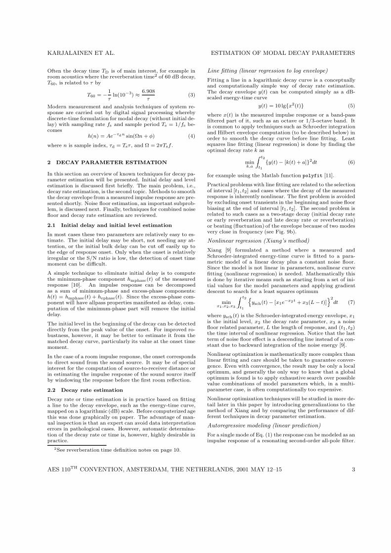
Estimation of Modal Decay Parameters from Noisy Response Measurements

Matti Karjalainen1, Poju Antsalo1, Aki Makivirta2, Timo Peltonen3, and Vesa Valimaki1

1Helsinki University of Technology, Laboratory of Acoustics and Audio Signal Processing,P.O. Box 3000, FIN-02015 HUT, Finland

2Genelec Oy, Iisalmi, Finland, and 3Akukon Oy, Helsinki, Finland

ABSTRACTEstimation of modal decay parameters from noisy measurements of reverberant and resonating systems is a commonproblem in audio and acoustics, e.g., in room and concert hall measurements or musical instrument modeling. In thispaper, reliable methods to estimate the initial response level, decay rate, and noise floor level from noisy measurementdata are studied and compared. A new method, based on nonlinear optimization of a model for exponential decayplus stationary noise floor, is presented. Comparison with traditional decay parameter estimation techniques usingsimulated measurement data shows that the proposed method outperforms in accuracy and robustness, especially inextreme SNR conditions. Three cases of practical applications of the method are demonstrated.

0 INTRODUCTION

Parametric analysis, modeling, and equalization (inversemodeling) of reverberant and resonating systems find manyapplications in audio and acoustics. These include room andconcert hall acoustics, resonators in musical instruments, andresonant behavior in audio reproduction systems. Estima-tion of reverberation time or modal decay rate are importantmeasurement problems in room and concert hall acoustics [1],where S/N ratios of only 30-50 dB are common. The sameproblems can be found for example in the estimation of pa-rameters in model-based sound synthesis of musical instru-

ments, such as vibrating strings or body modes of string in-struments [2]. Reliable methods to estimate parameters fromnoisy measurements are thus needed.

In an ideal case of modal behavior, after a possible initialtransient, the decay is exponential until a steady state noisefloor is encountered. The parameters of primary interest tobe estimated are:

- Initial level of decay (LI)- Decay rate/time or reverberation time (TD)- Noise floor level (LN)

In a more complex case there can be two or more modal fre-

KARJALAINEN ET AL. ESTIMATION OF MODAL DECAY PARAMETERS

quencies, whereby the decay is not simple anymore, but showsadditional fluctuation (beating) or a two-stage (or multiple-stage) decay behavior. In a diffuse field (room acoustics) thedecay of a noise-like response is approximately exponential inrooms with compact geometry. The noise floor may also benon-stationary. In this article we primarily discuss a simplemode (i.e., a complex conjugate pole pair in transfer function)or a dense set of modes with exponential reverberant decay,together with a stationary noise floor.

Methods presented in literature and common-sense or ad-hocmethods will first be reviewed. Techniques based on energy-time curve analysis of signal envelope are known as methodswhere the noise floor can be found and estimated explicitly.Backwards integration of energy, so called Schroeder integra-tion [3]-[4], is often applied first to obtain a smoothed enve-lope for decay rate estimation. AR modeling of modes byestimating the transfer function poles and group delay anal-ysis are examples of straightforward methods which are notparticularly robust against background noise.

The effect of background noise floor is known to be problem-atic, and techniques have been developed to compensate theeffect of envelope flattening when the noise floor in a mea-sured response is reached, including limiting the period ofintegration [5], subtracting an estimated noise floor energylevel from a response [6], or using two separate measurementsto reduce the effect of noise [7]. The iterative method by Lun-deby et al. [8] is of particular interest since it addresses withcare the case of noisy data. This technique, as most othermethods, analyzes the initial level LI, decay time TD, andnoise floor LN parameters separately, typically starting froma noise floor estimate. Iterative procedures are common inaccurate estimation.

A different approach was taken by Xiang [9] where aparametrized signal-plus-noise model is fitted to Schroeder-integrated measurement data by searching for a least squares(LS) optimal solution. In this study we have elaborated asimilar method of nonlinear LS optimization further to makeit applicable to a wide range of situations, showing good con-vergence properties. A specific parameter and/or a weight-ing function can be used to further fine-tune the method forspecific problems. The technique is compared with the Lun-deby et al. method by applying them to simulated cases ofexponential decay plus stationary noise floor where the exactparameters are known. The improved nonlinear optimizationtechnique is found to outperform traditional methods in accu-racy and robustness, particularly in difficult conditions withextreme signal-to-noise ratios.

Finally, the applicability of the improved method is demon-strated by three examples of real measurement data: (a) re-verberation time of a concert hall, (b) low-frequency modeanalysis of a room, and (c) parametric analysis of guitar stringbehavior for model-based sound synthesis. Possibilities forfurther generalization of the technique to more complex prob-lems, such as two-stage decay, will be discussed briefly.

1 DEFINITION OF PROBLEM DOMAIN

A typical property of resonant acoustic systems is that theirimpulse response is a decaying function after a possible initialdelay and the onset. In the simplest case the response of a

single mode resonator system is

h(t) = Ae−τ(t−t0) sin[ω(t − t0) + φ]u(t − t0) (1)

where u(t − t0) is a step function with value 1 for t ≥ t0and zero elsewhere, A is initial response level, t0 responselatency for example due to propagation delay of sound, τdecay rate parameter, ω = 2πf angular frequency, and φ ini-tial phase of sinusoidal response. In practical measurements,when there are multiple modes in the system and noise (acous-tic noise plus measurement system noise), a measured impulseresponse is of the form1

h(t) =

NXi=1

Aie−τi(t−t0) sin[ωi(t − t0) + φi] + Ann(t) (2)

where An is the rms value of background noise and n(t) isunity level noise signal. Figure 1 illustrates a single delayedmode response corrupted by additive noise.

-1

-0.5

0

0.5

1

-30

-25

-20

-15

-10

-5

0

dB

noise floor level

exponential decay (a)delay

noise floor level (LN)LN

initial level (IL) (b)

0 200 400 600 800 1000 1200 time in samples-30

-25

-20

-15

-10

-5

0

dB


initial level (IL) (b)


initial level (IL) (c)

Fig. 1: (a) Single mode impulse response (sinusoidal decay)with initial delay and additive measurement noise. (b) Abso-lute value of response on the dB scale to illustrate the decayenvelope. (c) Hilbert envelope, otherwise same as (b).

The problem of this study is defined as a task to find re-liable estimates for the parameter set Ai, τi, t0, ωi, φi,An,given a noisy measured impulse response of the form (2). Themain interest here is focused on systems of (a) separable sin-gle modes of type (1) including additive noise floor or (b)dense (diffuse, noiselike) set of modes resulting also in expo-nential decay similar to Fig. 1. In both cases the parametersof primary interest are A, τ,An, and t0.

1In a more general case the initial delays may differ and there can be simple non-modal exponential terms, but these casesare of less importance here.

AES 110TH CONVENTION, AMSTERDAM, THE NETHERLANDS, 2001 MAY 12–15 2


Often the decay time TD is of main interest, for example inroom acoustics where the reverberation time2 of 60 dB decay,T60, is related to τ by

T60 = − 1

τln(10−3) ≈ 6.908

τ(3)

Modern measurement and analysis techniques of system re-sponse are carried out by digital signal processing wherebydiscrete-time formulation for modal decay (without initial de-lay) with sampling rate fs and sample period Ts = 1/fs be-comes

h(n) = Ae−τdn sin(Ωn + φ) (4)

where n is sample index, τd = Tsτ , and Ω = 2πTsf .

2 DECAY PARAMETER ESTIMATION

In this section an overview of known techniques for decay pa-rameter estimation will be presented. Initial delay and levelestimation is discussed first briefly. The main problem, i.e.,decay rate estimation, is the second topic. Methods to smooththe decay envelope from a measured impulse response are pre-sented shortly. Noise floor estimation, an important subprob-lem, is discussed next. Finally, techniques for combined noisefloor and decay rate estimation are reviewed.

2.1 Initial delay and initial level estimation

In most cases these two parameters are relatively easy to es-timate. The initial delay may be short, not needing any at-tention, or the initial bulk delay can be cut off easily up tothe edge of response onset. Only when the onset is relativelyirregular or the S/N ratio is low, the detection of onset timemoment can be difficult.

A simple technique to eliminate initial delay is to computethe minimum-phase component hmphase(t) of the measuredresponse [10]. An impulse response can be decomposedas a sum of minimum-phase and excess-phase components:h(t) = hmphase(t) + hephase(t). Since the excess-phase com-ponent will have allpass properties manifested as delay, com-putation of the minimum-phase part will remove the initialdelay.

The initial level in the beginning of the decay can be detecteddirectly from the peak value of the onset. For improved ro-bustness, however, it may be better to estimate it from thematched decay curve, particularly its value at the onset timemoment.

In the case of a room impulse response, the onset correspondsto direct sound from the sound source. It may be of specialinterest for the computation of source-to-receiver distance orin estimating the impulse response of the sound source itselfby windowing the response before the first room reflection.

2.2 Decay rate estimation

Decay rate or time estimation is in practice based on fittinga line to the decay envelope, such as the energy-time curve,mapped on a logarithmic (dB) scale. Before computerized agethis was done graphically on paper. The advantage of man-ual inspection is that an expert can avoid data interpretationerrors in pathological cases. However, automatic determina-tion of the decay rate or time is, however, highly desirable inpractice.

Line fitting (linear regression to log envelope)

Fitting a line in a logarithmic decay curve is a conceptuallyand computationally simple way of decay rate estimation.The decay envelope y(t) can be computed simply as a dB-scaled energy-time curve

y(t) = 10 lgx2(t) (5)

where x(t) is the measured impulse response or a band-passfiltered part of it, such as an octave or 1/3-octave band. Itis common to apply techniques such as Schroeder integrationand Hilbert envelope computation (to be described below) inorder to smooth the decay curve before line fitting. Leastsquares line fitting (linear regression) is done by finding theoptimal decay rate k as

mink,a

Z t2

t1

y(t) − [k(t) + a]2dt (6)

for example using the Matlab function polyfit [11].

Practical problems with line fitting are related to the selectionof interval [t1, t2] and cases where the decay of the measuredresponse is inherently nonlinear. The first problem is avoidedby excluding onset transients in the beginning and noise floorbiasing at the end of interval [t1, t2]. The second problem isrelated to such cases as a two-stage decay (initial decay rateor early reverberation and late decay rate or reverberation)or beating (fluctuation) of the envelope because of two modesvery close in frequency (see Fig. 9b).

Nonlinear regression (Xiang’s method)

Xiang [9] formulated a method where a measured andSchroeder-integrated energy-time curve is fitted to a para-metric model of a linear decay plus a constant noise floor.Since the model is not linear in parameters, nonlinear curvefitting (nonlinear regression) is needed. Mathematically thisis done by iterative means such as starting from a set of ini-tial values for the model parameters and applying gradientdescent to search for a least squares optimum

minx1 ,x2 ,x3

Z t2

t1

nysch(t) − [x1e−x2t + x3(L − t)]

o2dt (7)

where ysch(t) is the Schroeder-integrated energy envelope, x1

is the initial level, x2 the decay rate parameter, x3 a noisefloor related parameter, L the length of response, and (t1, t2)the time interval of nonlinear regression. Notice that the lastterm of noise floor effect is a descending line instead of a con-stant due to backward integration of the noise energy [9].

Nonlinear optimization is mathematically more complex thanlinear fitting and care should be taken to guarantee conver-gence. Even with convergence, the result may be only a localoptimum, and generally the only way to know that a globaloptimum is found is to apply exhaustive search over possiblevalue combinations of model parameters which, in a multi-parameter case, is often computationally too expensive.

Nonlinear optimization techniques will be studied in more de-tail later in this paper by introducing generalizations to themethod of Xiang and by comparing the performance of dif-ferent techniques in decay parameter estimation.

Autoregressive modeling (linear prediction)

For a single mode of Eq. (1) the response can be modeled as animpulse response of a resonating second-order all-pole filter.

2See reverberation time definition notes on page 10.



More generally, a combination of N modes can be modeledas a 2N -order all-pole filter. Auto-regressive (AR) model-ing [12] is a way to derive parameters for such a model. Inmany technical applications this method is called linear pre-diction [13]. For example the function lpc in Matlab [14]processes a signal frame through autocorrelation coefficientcomputation and solving the normal equations by Levinsonrecursion, resulting in a N th order z-domain transfer func-

tion 1/(1 +PN

i=1 αiz−i). Poles are obtained by solving the

roots of the denominator polynomial. Each modal resonanceappears as a complex-conjugate pole pair (zi, z∗i ) in the com-plex z-plane with angle φ = arg(zi) = 2πf/fs and radius

r = |zi| = e−τ/fs , where f is modal frequency, fs is samplingrate, and τ is the decay parameter of the mode in Eq. (1).

Decay parameter analysis by AR modeling is not robust withlong decay times (poles close to the unit circle) and back-ground noise. Additive noise flattens the power spectrumof a modal resonance and moves the poles from unit circletowards the origin, thus resulting in shortened decay time es-timates, which is contrary to the result in linear curve fitting.AR modeling works for decay parameter estimation only if itcan spectrally resolve each mode. Thus it is not applicableto high modal densities, such as typical reverberation timemeasurements.

Group delay analysis

A complementary method to AR modeling is to use the groupdelay, i.e., phase derivative Tg(ω) = −dϕ(ω)/dω, as an esti-mate of the decay time for separable modes of an impulseresponse. While AR modeling is sensitive to power spectrumonly, the group delay is based on phase properties only. For aminimum-phase single mode response the group delay at themodal frequency is inversely proportional to the decay param-eter, i.e., Tg = 1/τ . Group delay computation is somewhatcritical due to phase unwrapping needed, and the method issensitive to measurement noise.

2.3 Decay envelope smoothing techniques

In the methods of linear or nonlinear curve fitting it is de-sirable to obtain a smooth decay envelope before the fittingoperation. The following techniques are often used to improvethe regularity of the decay ramp.

Hilbert envelope computation

In this method, signal x(t) is first converted to an analytic sig-nal xa(t) so that x(t) is the real part of xa(t) and the complexpart of xa(t) is the Hilbert transform (90o phase shift) [10] ofx(t). For a single sinusoid this results in an entirely smoothenergy-time envelope. An example of Hilbert envelope for anoisy modal response is shown in Fig. 1c.

Schroeder integration

A monotonic and smoothed decay curve can be produced by‘backward integration’ of the impulse response h(t) over mea-surement interval [0,T ] and converting it to a logarithmic scale

L(t) = 10 lg

R Tt h2(τ )dτR T0

h2(τ )dτ

![dB] (8)

This process is commonly known as the Schroeder integra-tion [3, 4]. Based on its superior smoothing properties it isused routinely in modern reverberation time measurements.

A known problem with it is that if the background noise flooris included within the integration interval, the process pro-duces a raised ramp that biases upwards the late part of de-cay. This is shown in Fig. 2 for the case of noisy single-modedecay of (a) for full response integration shown as curve (d).

-1

-0.5

0

0.5

1

0 200 400 600 800 1000 1200

-25

-20

-15

-10

-5

0

time in samples

dB

(a)

(b) (d)

(e) (f)(c)

(g)

(b)

0 200 400 600 800 1000 1200

-25

-20

-15

-10

-5

0

time in samples

0 200 400 600 800 1000 1200 time in samples

dB

(h)

Fig. 2: Results of Schroeder integration applied to noisy de-cay of a mode: (a) measured noisy response including ini-tial delay, (b) true decay of noiseless mode (dashed straightline), (c) noise floor (-26 dB), (d) Schroeder integration oftotal measured interval, (e) integration over a short interval(0,900), (f) integration over interval (0,1100), (g) integrationafter subtracting noise floor from energy-time curve, and (h)a few decay curves integrated by the Hirata’s method.

The tail problem of Schroeder integration has been addressedby many authors, for example in [15, 8, 5, 6], and techniquesto reduce slope biasing have been proposed. In order to applythese improvements, a good estimate of the noise floor levelis needed first.

2.4 Noise floor level estimation

The limited signal-to-noise ratio inherent in practically allacoustical measurements, and especially measurements per-formed under field conditions, call for attention concerningthe upper time limit of decay curve fitting or Schroeder in-tegration. Theoretically this limit is set to infinity, but inpractical measurements it is naturally limited to the lengthof the measured impulse response data. In practice, measuredimpulse responses must be long enough to accommodate forlarge enough dynamic range or the whole system decay downto the background noise level3.

Thus the measured impulse response typically contains notonly the decay curve under analysis, but also a steady level ofbackground noise, which dominates for some time at the endof the response. Fitting the decay line over this part of en-velope or Schroeder integrating this steady energy level along

3This is needed to avoid time aliasing with MLS and other cyclic impulse response measurement methods.



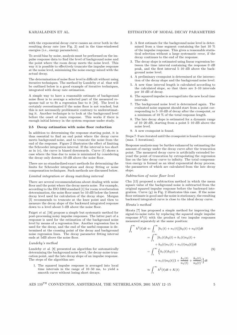
with the exponential decay curve causes an error both in theresulting decay rate (see Fig. 2) and in the time-windowedenergies (i.e., energy parameters).

To avoid bias by noise, analysis must be performed on the im-pulse response data to find the level of background noise andthe point where the room decay meets the noise level. Thisway it is possible to effectively truncate the impulse responseat the noise level, minimizing the noise energy mixed with theactual decay.

The determination of noise floor level is difficult without usingiterative techniques. The method by Lundeby et al. that willbe outlined below is a good example of iterative techniques,integrated with decay rate estimation.

A simple way to have a reasonable estimate of backgroundnoise floor is to average a selected part of the measured re-sponse tail or to fit a regression line to it [16]. The level iscertainly overestimated if the noise floor is not reached, butthis is not necessarily problematic contrary to underestimat-ing it. Another technique is to look at the background levelbefore the onset of main response. This works if there isenough initial latency in the system response under study.

2.5 Decay estimation with noise floor reduction

In addition to determining the response starting point, it isthus essential to find an end point where the decay curvemeets background noise, and to truncate the noise from theend of the response. Figure 2 illustrates the effect of limitingthe Schroeder integration interval. If the interval is too shortas in (e), the curve is biased downwards. Curve (f) shows acase where the bias due to noise is minimized by consideringthe decay only downto 10 dB above the noise floor.

There are no standardized exact methods for determining thelimits for Schroeder integration and decay fitting or noisecompensation techniques. Such methods are discussed below.

Limited integration or decay matching interval

There are several recommendations about dealing with noisefloor and the point where the decay meets noise. For example,according to the ISO 3382 standard [1] for room reverberationdetermination, the noise floor must be 10 dB below the lowestdecay level used for calculation of the decay slope. Morgan[5] recommends to truncate at the knee point and then tomeasure the decay slope of the backward integrated responsedown to a level about 5 dB above the noise floor.

Faiget et al. [16] propose a simple but systematic method forpost-processing noisy impulse responses. The latter part of aresponse is used for the estimation of the background noiselevel by means of a regression line. Another regression line isused for the decay, and the end of the useful response is de-termined at the crossing point of the decay and backgroundnoise regression lines. The decay parameter fitting intervalends at 5dB above the noise floor.

Lundeby’s method

Lundeby et al. [8] presented an algorithm for automaticallydetermining the background noise level, the decay-noise trun-cation point, and the late decay slope of an impulse response.The steps of the algorithm are:

1. The squared impulse response is averaged into localtime intervals in the range of 10–50 ms, to yield asmooth curve without losing short decays.

2. A first estimate for the background noise level is deter-mined from a time segment containing the last 10 %of the impulse response. This gives a reasonable statis-tical selection without a large systematic error, if thedecay continues to the end of the response.

3. The decay slope is estimated using linear regression be-tween the time interval containing the response 0 dBpeak, and the first interval 5–10 dB above the back-ground noise level.

4. A preliminary crosspoint is determined at the intersec-tion of the decay slope and the background noise level.

5. A new time interval length is calculated according tothe calculated slope, so that there are 3–10 intervalsper 10 dB of decay.

6. The squared impulse is averaged into the new local timeintervals.

7. The background noise level is determined again. Theevaluated noise segment should start from a point cor-responding to 5–10 dB of decay after the crosspoint, ora minimum of 10 % of the total response length.

8. The late decay slope is estimated for a dynamic rangeof 10–20 dB, starting from a point 5–10 dB above thenoise level.

9. A new crosspoint is found.

Steps 7–9 are iterated until the crosspoint is found to converge(max. 5 iterations).

Response analysis may be further enhanced by estimating theamount of energy under the decay curve after the truncationpoint. The measured decay curve is artificially extended be-yond the point of truncation by extrapolating the regressionline on the late decay curve to infinity. The total compensa-tion energy is formed as an ideal exponential decay process,the parameters of which are calculated from the late decayslope.

Subtraction of noise floor level

Chu [15] proposed a subtraction method in which the meansquare value of the background noise is subtracted from theoriginal squared impulse response before the backward inte-gration. Curve (g) in Fig. 2 illustrates this case. If the noisefloor estimate is good and the noise is stationary, the resultingbackward integrated curve is close to the ideal decay curve.

Hirata’s method

Hirata [7] has proposed a simple method for improving thesignal-to-noise ratio by replacing the squared single impulseresponse h2(t) with the product of two impulse responsesmeasured separately at the same position:Z ∞

th2(t)dt ⇐

Z ∞

t[h1(t) + n1(t)][h2(t) + n2(t)]dt

=

Z ∞

t[h1(t)h2(t) + h1(t)n2(t) +

+ h2(t)n1(t) + n1(t)n2(t)]dt

=

Z ∞

t

nh1(t)h2(t) +

+ n1(t)n2(t)[1 +h1(t)

n1(t)+

h2(t)

n2(t)]o

dt

≈Z ∞

th2(t)dt + K(t)

(9)



The measured impulse responses consist of the decay termsh1(t), h2(t) and the noise terms n1(t), n2(t). The highlycorrelated decay terms h1(t) and h2(t) yield positive valuescorresponding to squared response h2(t), whereas the mutu-ally uncorrelated noise terms n1(t) and n2(t) are seen as arandom fluctuation K(t) superposed on the first term.

Curves (h) in Fig. 2 illustrate a few decay curves obtainedby backward integration with Hirata’s method. In this simu-lated case they correspond to the case of (g), the noise floorsubtraction technique.

Other methods

Under adverse noise conditions, a direct determination of theT30 decay curve from the squared and time-averaged impulseresponse has been noted to be more robust than the backwardintegration method (Satoh et al. [17]).

3 NONLINEAR OPTIMIZATION OF A DECAY-PLUS-NOISE MODEL

The nonlinear regression (optimization) method proposed byXiang [9] was shortly described above. In the present studywe have worked along similar ideas, using nonlinear optimiza-tion for improved robustness and accuracy. Below we intro-duce the nonlinear decay-plus-noise model and its applicationin several cases.

Let us assume that in noiseless conditions the system understudy results in simple exponential decay of response enve-lope, corrupted by additive stationary background noise. Wewill study two cases that fit into the same model category.In the first case there is a single mode (i.e., a complex conju-gate pole pair in transfer function) that in the time domaincorresponds to an exponential decay function

hm(t) = Ame−τmt sin(ωmt + φm) (10)

Here Am is the initial envelope amplitude of the decaying si-nusoidal, τm is a coefficient that defines the decay rate, ωm

is the angular frequency of the mode, and φm is the initialphase of modal oscillation.

The second case that leads to a similar formulation is wherewe have a high density of modes (diffuse sound field) with ex-ponential decay, resulting in an exponentially decaying noise

hd(t) = Ade−τdtn(t) (11)

where Ad is the initial rms level of response, τd is a decayrate parameter, and n(t) is stationary Gaussian noise withrms level of 1 (= 0 dB).

In both Eqs. (10) and (11) we assume that a practical mea-surement of the system impulse response is corrupted withadditive stationary noise

nb(t) = Ann(t) (12)

where An is the rms level of Gaussian measurement noise onthe analysis bandwidth of interest, and it is assumed to beuncorrelated with the decaying system response. Statisticallythe rms envelope of the measured response is then

a(t) =q

h2(t) + n2b(t) =

qA2e−2τt + A2

n (13)

This is a simple decay model that can be used for parametricanalysis of noise-corrupted measurements. If the amplitude

envelope of a specific measurement is y(t), then optimizedleast squares (LS) error estimate for parameters A, τ,Ancan be achieved by minimizing the following expression overa time span [t0, t1] of interest

minA,τ,An

Z t1

t0

[a(t)− y(t)]2dt (14)

Since the model of Eq. (13) is nonlinear in parametersA, τ,An, nonlinear LS optimization is needed to search forthe minimum LS error.

By numerical experimentation with real measurement data itis easy to observe that LS fitting of the model of Eq. (14)places emphasis on large magnitude values, whereby noisefloors well below the signal starting level are estimated poorly.In order to improve the optimization, a generalized form ofmodel fitting can be formulated by minimization

minA,τ,An

Z t1

t0

nf(a(t), t) − f(y(t), t)

o2dt (15)

where f(y, t) is a mapping to balance weight for different en-velope level values and time moments.

The choice of f(y, t) = 20 log(y(t)) results in fitting on thedecibel scale. It turns out that low-level noise easily hasa dominating role in this formulation. A better result inmodel fitting can be achieved by using a power law scalingf(y, t) = ys(t) with factor s < 1, which is a compromise be-tween amplitude vs. logarithmic scaling. A value of s ≈ 0.5has been found a useful default value4.

A time-dependent part of mapping f(y, t), if needed, can beseparated as a temporal weighting function w(t). A general-ized form of the entire optimization is now to find

minA,τ,An

Z t1

t0

nw(t)as(t) − w(t)ys(t)

o2dt (16)

There is no clear physical motivation for the magnitude com-pression factor s. Specific temporal weighting functions w(t)can be applied case by case, based on extra knowledge on thebehavior of the system under study and goals of the analysis,such as focusing on the early decay time (early reverberation)of a room response.

The strengths of the nonlinear optimization method are ap-parent especially under extreme SNR conditions where allthree parameters, A, τ,An, are needed with the best ac-curacy. This occurs both at very low SNR conditions wherethe signal is practically buried in background noise and at theother extreme where the noise floor is not reached within themeasured impulse response but still an estimate of the noiselevel is desired. The necessary assumption for the method towork in such cases is that the decay model is valid, implyingan exponential decay and stationary noise floor. Experimentsshow the method to work both for single mode decay andreverberant acoustic field decay models.

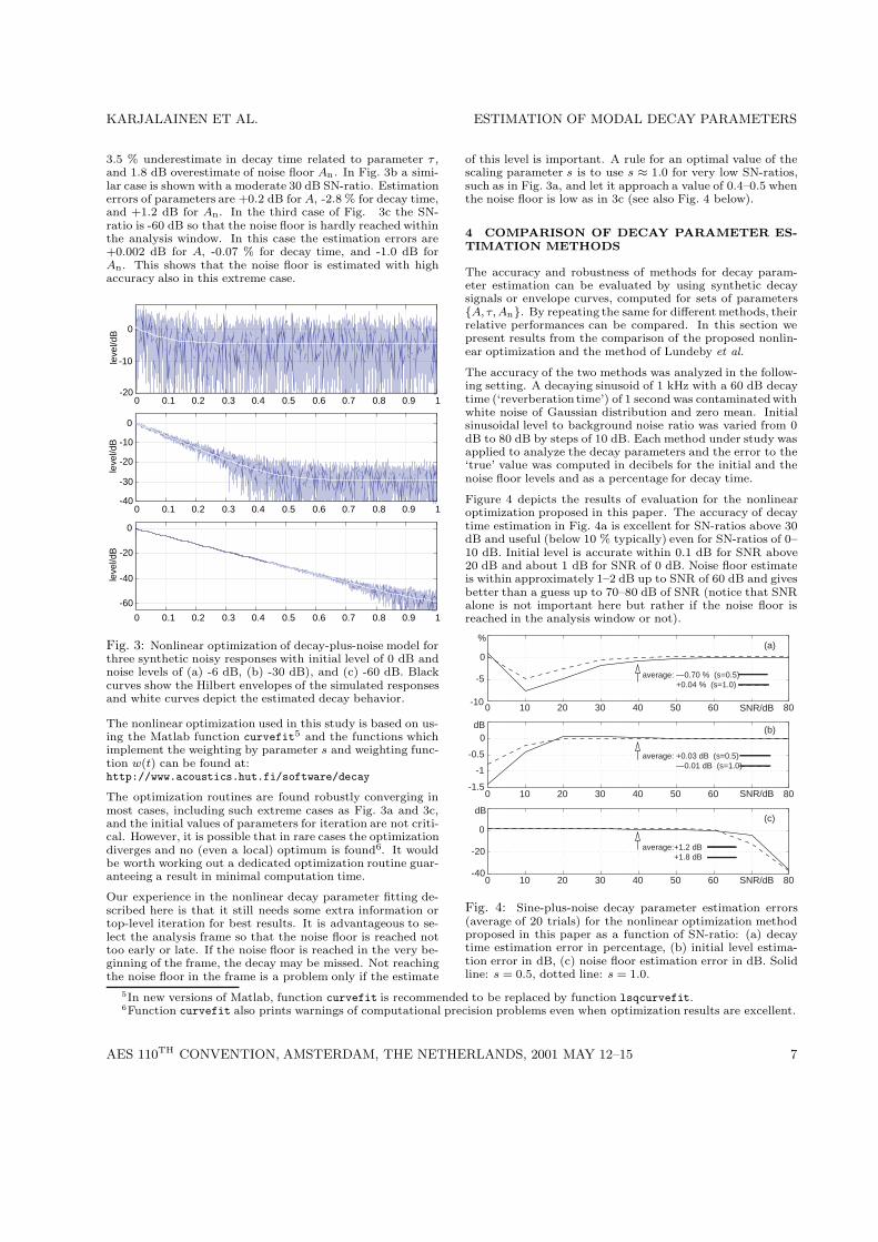
Figure 3 depicts three illustrative examples of decay modelfitting of a single mode at an initial level of 0 dB and differ-ent noise floor levels. Because of simulated noisy responses itis easy to evaluate the estimation accuracy of each parameter.White curves show the estimated behavior of the decay-plus-noise model. In Fig. 3a the SN-ratio is only 6 dB. Errors inparameters in this case are a 0.5 dB underestimation of A,

4Interestingly enough, this is close to the loudness scaling in auditory perception known from psychoacoustics [18].



3.5 % underestimate in decay time related to parameter τ ,and 1.8 dB overestimate of noise floor An . In Fig. 3b a simi-lar case is shown with a moderate 30 dB SN-ratio. Estimationerrors of parameters are +0.2 dB for A, -2.8 % for decay time,and +1.2 dB for An. In the third case of Fig. 3c the SN-ratio is -60 dB so that the noise floor is hardly reached withinthe analysis window. In this case the estimation errors are+0.002 dB for A, -0.07 % for decay time, and -1.0 dB forAn. This shows that the noise floor is estimated with highaccuracy also in this extreme case.

0 0.1 0.2 0.3 0.4 0.5 0.6 0.7 0.8 0.9 1-20

-10

0

leve

l/dB

0 0.1 0.2 0.3 0.4 0.5 0.6 0.7 0.8 0.9 1-40

-30

-20

-10

0

leve

l/dB

0 0.1 0.2 0.3 0.4 0.5 0.6 0.7 0.8 0.9 1

-60

-40

-20

0

leve

l/dB

Fig. 3: Nonlinear optimization of decay-plus-noise model forthree synthetic noisy responses with initial level of 0 dB andnoise levels of (a) -6 dB, (b) -30 dB), and (c) -60 dB. Blackcurves show the Hilbert envelopes of the simulated responsesand white curves depict the estimated decay behavior.

The nonlinear optimization used in this study is based on us-ing the Matlab function curvefit5 and the functions whichimplement the weighting by parameter s and weighting func-tion w(t) can be found at:http://www.acoustics.hut.fi/software/decay

The optimization routines are found robustly converging inmost cases, including such extreme cases as Fig. 3a and 3c,and the initial values of parameters for iteration are not criti-cal. However, it is possible that in rare cases the optimizationdiverges and no (even a local) optimum is found6. It wouldbe worth working out a dedicated optimization routine guar-anteeing a result in minimal computation time.

Our experience in the nonlinear decay parameter fitting de-scribed here is that it still needs some extra information ortop-level iteration for best results. It is advantageous to se-lect the analysis frame so that the noise floor is reached nottoo early or late. If the noise floor is reached in the very be-ginning of the frame, the decay may be missed. Not reachingthe noise floor in the frame is a problem only if the estimate

of this level is important. A rule for an optimal value of thescaling parameter s is to use s ≈ 1.0 for very low SN-ratios,such as in Fig. 3a, and let it approach a value of 0.4–0.5 whenthe noise floor is low as in 3c (see also Fig. 4 below).

4 COMPARISON OF DECAY PARAMETER ES-TIMATION METHODS

The accuracy and robustness of methods for decay param-eter estimation can be evaluated by using synthetic decaysignals or envelope curves, computed for sets of parametersA, τ,An. By repeating the same for different methods, theirrelative performances can be compared. In this section wepresent results from the comparison of the proposed nonlin-ear optimization and the method of Lundeby et al.

The accuracy of the two methods was analyzed in the follow-ing setting. A decaying sinusoid of 1 kHz with a 60 dB decaytime (‘reverberation time’) of 1 second was contaminated withwhite noise of Gaussian distribution and zero mean. Initialsinusoidal level to background noise ratio was varied from 0dB to 80 dB by steps of 10 dB. Each method under study wasapplied to analyze the decay parameters and the error to the‘true’ value was computed in decibels for the initial and thenoise floor levels and as a percentage for decay time.

Figure 4 depicts the results of evaluation for the nonlinearoptimization proposed in this paper. The accuracy of decaytime estimation in Fig. 4a is excellent for SN-ratios above 30dB and useful (below 10 % typically) even for SN-ratios of 0–10 dB. Initial level is accurate within 0.1 dB for SNR above20 dB and about 1 dB for SNR of 0 dB. Noise floor estimateis within approximately 1–2 dB up to SNR of 60 dB and givesbetter than a guess up to 70–80 dB of SNR (notice that SNRalone is not important here but rather if the noise floor isreached in the analysis window or not).

0 10 20 30 40 50 60 80-10

-5

0

%

0 10 20 30 40 50 60 80-1.5

-1

-0.5

0dB

0 10 20 30 40 50 60 SNR/dB

SNR/dB

SNR/dB

80-40

-20

0

dB

average:+1.2 dB +1.8 dB

average: +0.03 dB (s=0.5) —0.01 dB (s=1.0)

average: —0.70 % (s=0.5) +0.04 % (s=1.0)

(a)

(b)

(c)

Fig. 4: Sine-plus-noise decay parameter estimation errors(average of 20 trials) for the nonlinear optimization methodproposed in this paper as a function of SN-ratio: (a) decaytime estimation error in percentage, (b) initial level estima-tion error in dB, (c) noise floor estimation error in dB. Solidline: s = 0.5, dotted line: s = 1.0.

5In new versions of Matlab, function curvefit is recommended to be replaced by function lsqcurvefit.6Function curvefit also prints warnings of computational precision problems even when optimization results are excellent.



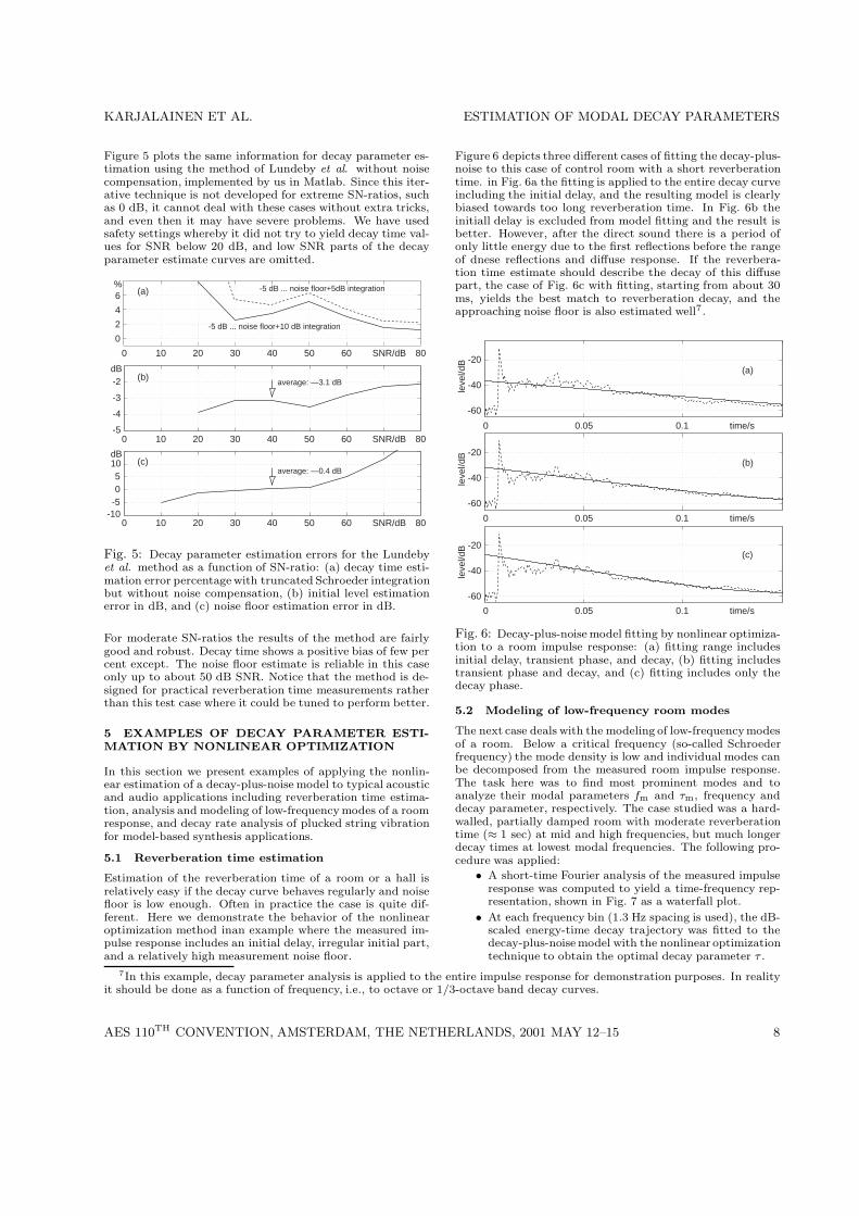
Figure 5 plots the same information for decay parameter es-timation using the method of Lundeby et al. without noisecompensation, implemented by us in Matlab. Since this iter-ative technique is not developed for extreme SN-ratios, suchas 0 dB, it cannot deal with these cases without extra tricks,and even then it may have severe problems. We have usedsafety settings whereby it did not try to yield decay time val-ues for SNR below 20 dB, and low SNR parts of the decayparameter estimate curves are omitted.

-5

-4

-3

-2

-505

10dB

dB

0 10 20 30 40 50 60 SNR/dB 80-10

0 10 20 30 40 50 60 SNR/dB 80

0 10 20 30 40 50 60 SNR/dB 80

(b)

(c)

average: —3.1 dB

average: —0.4 dB

0

2

4

6%

(a)

-5 dB ... noise floor+10 dB integration

-5 dB ... noise floor+5dB integration

Fig. 5: Decay parameter estimation errors for the Lundebyet al. method as a function of SN-ratio: (a) decay time esti-mation error percentage with truncated Schroeder integrationbut without noise compensation, (b) initial level estimationerror in dB, and (c) noise floor estimation error in dB.

For moderate SN-ratios the results of the method are fairlygood and robust. Decay time shows a positive bias of few percent except. The noise floor estimate is reliable in this caseonly up to about 50 dB SNR. Notice that the method is de-signed for practical reverberation time measurements ratherthan this test case where it could be tuned to perform better.

5 EXAMPLES OF DECAY PARAMETER ESTI-MATION BY NONLINEAR OPTIMIZATION

In this section we present examples of applying the nonlin-ear estimation of a decay-plus-noise model to typical acousticand audio applications including reverberation time estima-tion, analysis and modeling of low-frequency modes of a roomresponse, and decay rate analysis of plucked string vibrationfor model-based synthesis applications.

5.1 Reverberation time estimation

Estimation of the reverberation time of a room or a hall isrelatively easy if the decay curve behaves regularly and noisefloor is low enough. Often in practice the case is quite dif-ferent. Here we demonstrate the behavior of the nonlinearoptimization method inan example where the measured im-pulse response includes an initial delay, irregular initial part,and a relatively high measurement noise floor.

Figure 6 depicts three different cases of fitting the decay-plus-noise to this case of control room with a short reverberationtime. in Fig. 6a the fitting is applied to the entire decay curveincluding the initial delay, and the resulting model is clearlybiased towards too long reverberation time. In Fig. 6b theinitiall delay is excluded from model fitting and the result isbetter. However, after the direct sound there is a period ofonly little energy due to the first reflections before the rangeof dnese reflections and diffuse response. If the reverbera-tion time estimate should describe the decay of this diffusepart, the case of Fig. 6c with fitting, starting from about 30ms, yields the best match to reverberation decay, and theapproaching noise floor is also estimated well7.

0 0.05 0.1 time/s

0 0.05 0.1 time/s

0 0.05 0.1 time/s

-60

-40

-20

leve

l/dB

-60

-40

-20le

vel/d

B

-60

-40

-20

leve

l/dB

(a)

(b)

(c)

Fig. 6: Decay-plus-noise model fitting by nonlinear optimiza-tion to a room impulse response: (a) fitting range includesinitial delay, transient phase, and decay, (b) fitting includestransient phase and decay, and (c) fitting includes only thedecay phase.

5.2 Modeling of low-frequency room modes

The next case deals with the modeling of low-frequency modesof a room. Below a critical frequency (so-called Schroederfrequency) the mode density is low and individual modes canbe decomposed from the measured room impulse response.The task here was to find most prominent modes and toanalyze their modal parameters fm and τm, frequency anddecay parameter, respectively. The case studied was a hard-walled, partially damped room with moderate reverberationtime (≈ 1 sec) at mid and high frequencies, but much longerdecay times at lowest modal frequencies. The following pro-cedure was applied:

• A short-time Fourier analysis of the measured impulseresponse was computed to yield a time-frequency rep-resentation, shown in Fig. 7 as a waterfall plot.

• At each frequency bin (1.3 Hz spacing is used), the dB-scaled energy-time decay trajectory was fitted to thedecay-plus-noise model with the nonlinear optimizationtechnique to obtain the optimal decay parameter τ .

7In this example, decay parameter analysis is applied to the entire impulse response for demonstration purposes. In realityit should be done as a function of frequency, i.e., to octave or 1/3-octave band decay curves.



• Based on decay parameter values and spectral levels, arule was written to pick up the most prominent modalfrequencies and the related decay parameter values.

Fig. 7: Time-frequency plot of room response at low frequen-cies. Lowest modes (especially 40 Hz) show long decay times.

In this context we are interested in how well the decay pa-rameter estimation works with noisy measurements. Appli-cation of the nonlinear optimization resulted in decay param-eter estimates, some of which are illustrated in Fig. 8 by acomparison of the original decay and decay-plus-noise modelbehavior. For all frequencies in the vicinity of a mode themodel fits robustly and accurately.

0 0.5 1 1.5 2 2.5 3 3.5 4 time/s 5

0 0.5 1 1.5 2 2.5 3 3.5 4 time/s 5

0 0.5 1 1.5 2 2.5 3 3.5 4 time/s 5

-60

-40

-20

leve

l/dB

-80

-60

-40

leve

l/dB

-80

-60

-40

leve

l/dB

(a)

(b)

(c)

Fig. 8: Fitting of decay-plus-noise model to low-frequencymodal data of a room (see Fig. 7): (a) at 40 Hz mode, (b) at104 Hz, and (c) at 117 Hz (off-mode fast decay). Dotted line:measured, dashed line: modeled.

5.3 Analysis of decay rate of plucked string tones

Model-based synthesis of string tones can produce realisticguitar-like tones if the parameter values of the synthesis modelare calibrated based on recordings [2]. The main properties

of tones that need to be analyzed are their fundamental fre-quency and the decay time of all harmonic partials that areaudible. While the estimation of fundamental frequency isquite easy, the measurement of decay times of harmonics (=modes of the string) is complicated by the fact that they allhave a different rate of decay and also the initial level canvary within a range of 20-30 dB. There may also not be in-formation about the noise floor level for all harmonics.

One method used for measuring the decay times is based onthe short-time Fourier analysis. A recorded single guitar toneis sliced into frames with a window function in the time do-main. Each window function is then Fourier transformedwith the FFT using zero-padding to increase the spectralresolution, and harmonic peaks are hunted from the mag-nitude spectrum using a peak-picking algorithm. The peakvalues from the consecutive frames are organized as tracks,which correspond to the temporal envelopes of the harmon-ics. Then it becomes possible to estimate the decay rate ofeach harmonic mode. In the following, we show how thisworks with the proposed algorithm. Finally, the decay rateof each harmonic is converted into a corresponding target re-sponse, which is used for designing the magnitude responseof a digital filter that controls the decay of harmonics in thesynthesis model.

Figure 9 plots three examples of modal decay analysis of gui-tar string harmonics (string 5, open string plucking). Har-monic envelope trajectories were analyzed as described above.The decay-plus-noise model was fitted in a time window thatstarted from the maximum value position of the envelopecurve. In case (a), the second harmonic shows a highly reg-ular decay after initial transient of plucking whereby decayfitting is almost perfect. Case (b), harmonic number 24, de-picts a strongly beating decay where probably the horizontaland vertical polarizations have a frequency difference that af-ter summation results in beating. Case (c), harmonic 54,shows a harmonic trajectory where the noise floor is reachedwithin the analysis window. In all shown cases, the nonlinearoptimization works as perfectly as a simple decay model cando.

-20

-15

-10

-5

0

leve

l/dB

-20

-15

-10

-5

0

leve

l/dB

0 0.05 0.1 0.15 0.2 0.25 0.3 0.35 0.4 time/s

0 0.05 0.1 0.15 0.2 0.25 0.3 0.35 0.4 time/s

0 0.05 0.1 0.15 0.2 0.25 0.3 0.35 0.4 time/s

-50-40-30-20-10

0

leve

l/dB

(a)

(b)

(c)

Fig. 9: Examples of modal decay matching for harmonic com-ponents of a guitar string: (a) regular decay after initial tran-sient, (b) strongly beating decay (double mode), and (c) fastdecay that reaches the noise floor. Dotted line: measuredenvelope, solid line: optimized fit.



As can be concluded from case (b) of Fig. 9, a string canexhibit more complicated behavior than a simple exponen-tial decay. Even more complex is the case of piano tonesbecause there are 2–3 strings slightly off-tuned, and the en-velope fluctuation can be more irregular. Two-stage decay isalso common where the initial decay is faster than later decay.

In all such cases a more complex decay model is needed toachieve a good match with the measured data. It remains afuture problem to investigate fitting such models using linearoptimization techniques.

6 SUMMARY AND CONCLUSIONS

In this paper, an overview of modal decay analysis meth-ods for noisy impulse response measurements of reverberantacoustic systems is presented, and further improvements areintroduced. The problem of decay time determination is im-portant for example in room acoustics for characterizing thereverberation time. Another application where a similar prob-lem is encountered is when estimating string model parame-ters for model-based synthesis of plucked string instruments.

It is shown in this article that the further developments of thedecay-plus-noise model yield highly accurate decay parame-ter estimates, outperforming traditional methods especiallyunder extreme SN-ratio conditions. Challenges for furtherstudies remain to make the method (with increased numberof parameters) able to analyze complex decay characteristics,such as double decay behavior and strongly fluctuating re-sponses due to two or more modes very close in frequency.

The Matlab code for nonlinear optimization of decay parame-tres, including data examples, can be found at:http://www.acoustics.hut.fi/software/decay

ACKNOWLEDGMENTS

This study is part of the VARE technology program, projectTAKU (Control of Closed Space Acoustics), funded by Tekes(National Technology Agency). The work of Vesa Valimakihas been financed by the Academy of Finland.

Notes on reverberation time definitionsReverberation time T60 or just T is defined as the time in sec-onds it takes for the energy in the steady-state sound field ina room to decay 60 dB after the source of sound excitation issuddenly turned off [19]. According to definition by Beranek[20], the reverberation time might be defined in any of thefollowing ways:

1. the interval between turning off the sound source andthe time when the instantaneous value of the pressurelevel first falls to 60 dB below its steady state value

2. the time interval until the average value of the fluctu-ating pressure first falls to this value

3. the time until the average value of the fluctuating logp decay curve first falls to 60 dB below its steady statevalue, or

4. the time required for the evaluated decay slope to dropoff 60 dB.

In practice, the reverberation time is often determined fromthe slope of a decay curve using only the first 25 or 35 dBof decay and extrapolating the result to 60 dB. For the rec-ommended practice of reverberation time determination, seestandard [1].

REFERENCES

[1] ISO 3382-1997, Acoustics – Measurement of the Rever-beration Time of Rooms with Reference to Other Acous-tical Parameters. Geneva, Switzerland: InternationalStandards Organization, 1997. 21 p.

[2] V. Valimaki, J. Huopaniemi, M. Karjalainen, andZ. Janosy, “Physical Modeling of Plucked String Instru-ments with Application to Real-Time Sound Synthesis,”J. Audio Eng. Soc., vol. 44, no. 5, pp. 331–353, 1996May.

[3] M. R. Schroeder, “New Method of Measuring Reverber-ation Time,” J. Acoust. Soc. Am., vol. 37, pp. 409–412,1965.

[4] M. R. Schroeder, “Integrated-impulse Method Measur-ing Sound Decay Without Using Impulses,” J. Acoust.Soc. Am., vol. 66, no. 2, pp. 497–500, 1979 Aug.

[5] D. Morgan, “A parametric error analysis of the backwardintegration method for reverberation time estimation,”J. Acoust. Soc. Am., vol. 101, no. 5, pp. 2686–2693, 1997May.

[6] L. Faiget, C. Legros, and R. Ruiz, “Optimization ofthe Impulse Response Length: Application to Noisy andHighly Reverberant Rooms,” J. Audio Eng. Soc., vol. 46,no. 9, pp. 741–749, 1998 Sept.

[7] Y. Hirata, “A Method of Eliminating Noise in PowerResponses,” J. Sound Vib., vol. 82, no. 4, pp. 593–595,1982.

[8] A. Lundeby, T. E. Vigran, H. Bietz, and M. Vorlander,“Uncertainties of Measurements in Room Acoustics,”Acustica, vol. 81, pp. 344–355, 1995.

[9] N. Xiang, “Evaluation of Reverberation Times Using aNonlinear Regression Approach,” J. Acoust. Soc. Am.,vol. 98, no. 4, pp. 2112–2121, 1995 Oct.

[10] A. V. Oppenheim and R. W. Schafer, Digital Signal Pro-cessing. Englewood Cliffs, N.J.: Prentice-Hall, 1975.(Chapter 10, pp. 480–531).

[11] MathWorks, Inc., MATLAB User’s Guide, 2001.

[12] S. M. Kay, Fundamentals of Statistical Signal Process-ing: Volume I: Estimation Theory. Englewood Cliffs,N.J.: Prentice-Hall, 1993.

[13] J. D. Markel and J. A. H. Gray, Linear Prediction ofSpeech. Berlin, Germany: Springer-Verlag, 1976.

[14] MathWorks, Inc., MATLAB Signal Processing Toolbox,User’s Guide, 2001.

[15] W. T. Chu, “Comparison of reverberation measurementsusing Schroeder’s impulse method and decay-curve av-eraging method,” J. Acoust. Soc. Am., vol. 63, no. 5,pp. 1444–1450, 1978 May.

[16] L. Faiget, R. Ruiz, and C. Legros, “Estimation of Im-pulse Response Length to Compute Room AcousticalCriteria,” Acustica, vol. 82, no. Suppl. 1., p. S148, 1996Sept.

[17] F. Satoh, Y. Hidaka, and H. Tachibana, “ReverberationTime Directly Obtained from Squared Impulse ResponseEnvelope,” in Proc. Int. Congr. Acoust., vol. 4, (Seattle,WA), pp. 2755–2756, 1998 June.

[18] E. Zwicker and H. Fastl, Psychoacoustics — Facts andModels. Berlin: Springer-Verlag, 1990.

[19] W. C. Sabine, Architectural Acoustics. 1900. Reprint byDover, 1964, New York.

[20] L. Beranek, Acoustic Measurements. 1949. Reprint byAcoust. Soc. Am., 1988.


Estimation of Modal Decay Parameters from Noisy Response Measurements

Documents

Transcript of Estimation of Modal Decay Parameters from Noisy Response Measurements