Parameter Estimation of LPI Radar in Noisy Environments ...

IN DEGREE PROJECT COMPUTER SCIENCE AND ENGINEERING,SECOND CYCLE, 30 CREDITS

, STOCKHOLM SWEDEN 2021

Parameter Estimation of LPI Radar in Noisy Environments using Convolutional Neural Networks

FILIP APPELGREN

KTH ROYAL INSTITUTE OF TECHNOLOGYSCHOOL OF ELECTRICAL ENGINEERING AND COMPUTER SCIENCE

Parameter Estimation of LPIRadar in Noisy Environmentsusing Convolutional NeuralNetworks

FILIP APPELGREN

Master’s Programme, Computer Science, 120 creditsDate: July 8, 2021

Supervisor: Mats NordahlExaminer: Erik Fransén

School of Electrical Engineering and Computer ScienceHost company: Saab ABSwedish title: Parameteruppskattning av LPI radar i brusiga miljöermed faltningsnätverk

Abstract | i

AbstractLow-probability-of-intercept (LPI) radars are notoriously difficult forelectronic support receivers to detect and identify due to their changingradar parameters and low power. Previous work has been done to createautonomous methods that can estimate the parameters of some LPI radarsignals, utilizing methods outside of Deep Learning. Designs using theWigner-Ville Distribution in combination with the Hough and the Radontransform have shown some success. However, these methods lack fullautonomous operation, require intermediary steps, and fail to operate intoo low Signal-to-Noise ratios (SNR). An alternative method is presentedhere, utilizing Convolutional Neural Networks, with images created bythe Smoothed-Pseudo Wigner-Ville Distribution (SPWVD), to extractparameters. Multiple common LPI modulations are studied, frequencymodulated continuous wave (FMWC), Frank code and, Costas sequences.Five Convolutional Neural Networks (CNNs) of different sizes and layoutsare implemented to monitor estimation performance, inference time, andtheir relationship. Depending on how the parameters are represented, eitherwith continuous values or discrete, they are estimated through differentmethods, either regression or classification. Performance for the networks’estimations are presented, but also their inference times and potentialmaximum throughput of images.

The results indicate good performance for the largest networks, acrossmost variables estimated and over a wide range of SNR levels, with decayingperformance as network size decreases. The largest network achievesa standard deviation for the estimation errors of, at most, 6%, for theregression variables in the FMCW and the Frank modulations. For theparameters estimated through classification, accuracy is at least 56% over allmodulations. As network size decreases, so does the inference time. Thesmallest network achieves a throughput of about 61000 images per second,while the largest achieves 2600.

KeywordsDeep Learning, LPI, Radar, CNN, Parameter estimation

ii | Abstract

Sammanfattning | iii

SammanfattningLow-Probability-of-Intercept (LPI) radar är designad för att vara svåra attupptäcka och identifiera. En LPI radar uppnår detta genom att använda enlåg effekt samt ändra något hos radarsignalen över tid, vanligtvis frekvenseller fas. Estimering av parametrarna hos vissa typer av LPI radar har gjortsförut, med andra metoder än djupinlärning. De metoderna har använt sig avWigner-Ville Distributionen tillsammans med Hough och Radon transformerför att extrahera parametrar. Nackdelarna med dessa är framför allt att deinte fungerar fullständigt i för höga brusnivåer utan blir opålitliga i derasestimeringar. Utöver det kräver de också visst manuellt arbete, t.ex. i formav att sätta tröskelvärden. Här presenteras istället en metod som använderfaltningsnätverk tillsammans med bilder som genererats genom Smoothed-Pseudo Wigner-Ville Distributionen, för att estimera parametrarna hos LPIradar. Vanligt förekommande LPI-modulationer studeras, som frequencymodulated continuous wave (FMCW), Frank-koder och Costas-sekvenser.Fem faltningsnätverk av olika storlek implementeras, för att kunna studeraprestandan, analystiden per bild, och deras förhållande till varandra. Beroendepå hur parametrarna representeras, antingen med kontinuerliga värden ellerdiskreta värden, estimeras de med olika metoder, antingen regression ellerklassificering. Prestanda för nätverkens estimeringar presenteras, men ocksåderas analystid och potentiella maximala genomströmning av bilder.

Testen för parameterestimering visar på god prestanda, speciellt för destörre nätverken som studerats. För det största nätverket är standardavvikelsenpå estimeringsfelen som mest 6%, för FMCW- och Frank-modulationerna.För alla parametrar som estimeras genom klassificering uppnås som minst56% precision för det största nätverket. Även i testerna för analystid ärnätverksstorlek relevant. När storleken minskar, går antalet beräkningar sombehöver göras ned, och bilderna behandlas snabbare. Det minsta nätverketkan analysera ungefär 61000 bilder per sekund, medan det största uppnårungefär 2600 per sekund.

NyckelordDjupinlärning, LPI, Radar, Faltningsnätverk, Parameterestimering

iv | Sammanfattning

Acknowledgments | v

AcknowledgmentsMy thanks are firstly directed towards my fellow students and close friendsMåns Ekelund and Erik Båvenstrand. Thank you for the five years we haveput behind us, and thank you for the many years we have ahead.

Secondly, many thanks to Saab, Peter Sundström, and Daniel Franssonfor showing support not only during this thesis but for many years of work. Aspecial word of gratitude is directed towards Gustav Norén, who has sharedknowledge, experience, and discussions during this thesis.

Lastly, I would like to extend my thanks to my supervisor Mats Nordahl, who,with endless knowledge, has educated me not only in scientific subjects butalso in academic writing.

Stockholm, July 2021Filip Appelgren

vi | Acknowledgments

CONTENTS | vii

Contents

1 Introduction 11.1 Problem . . . . . . . . . . . . . . . . . . . . . . . . . . . . . 21.2 Purpose & Goal . . . . . . . . . . . . . . . . . . . . . . . . . 31.3 Methodology . . . . . . . . . . . . . . . . . . . . . . . . . . 31.4 Delimitations . . . . . . . . . . . . . . . . . . . . . . . . . . 41.5 Outline . . . . . . . . . . . . . . . . . . . . . . . . . . . . . . 4

2 Theoretical Background 72.1 Radar . . . . . . . . . . . . . . . . . . . . . . . . . . . . . . 7

2.1.1 IQ-Data . . . . . . . . . . . . . . . . . . . . . . . . . 82.2 Wigner-Ville Distribution . . . . . . . . . . . . . . . . . . . . 92.3 LPI-Modulations . . . . . . . . . . . . . . . . . . . . . . . . 11

2.3.1 Frequency Modulated Continuous Wave . . . . . . . . 112.3.2 Phase-Shift Keying . . . . . . . . . . . . . . . . . . . 122.3.3 Frequency-Shift Keying . . . . . . . . . . . . . . . . . 13

2.4 Deep Learning . . . . . . . . . . . . . . . . . . . . . . . . . . 152.4.1 Artificial Neuron . . . . . . . . . . . . . . . . . . . . 152.4.2 Loss function . . . . . . . . . . . . . . . . . . . . . . 162.4.3 Artificial Neural Networks . . . . . . . . . . . . . . . 162.4.4 Convolutional Neural Networks . . . . . . . . . . . . 182.4.5 Pooling . . . . . . . . . . . . . . . . . . . . . . . . . 192.4.6 Related Work . . . . . . . . . . . . . . . . . . . . . . 20

3 Methodology 233.1 Data generation . . . . . . . . . . . . . . . . . . . . . . . . . 233.2 Signals & Parameters . . . . . . . . . . . . . . . . . . . . . . 24

3.2.1 FMCW . . . . . . . . . . . . . . . . . . . . . . . . . 243.2.2 Frank Code . . . . . . . . . . . . . . . . . . . . . . . 253.2.3 Costas Code . . . . . . . . . . . . . . . . . . . . . . . 26

3.3 Implementation . . . . . . . . . . . . . . . . . . . . . . . . . 273.3.1 Architectures . . . . . . . . . . . . . . . . . . . . . . 28

viii | Contents

3.3.2 Setup . . . . . . . . . . . . . . . . . . . . . . . . . . 313.4 Evaluation . . . . . . . . . . . . . . . . . . . . . . . . . . . . 31

3.4.1 Regression . . . . . . . . . . . . . . . . . . . . . . . 313.4.2 Classification . . . . . . . . . . . . . . . . . . . . . . 34

3.5 Testing . . . . . . . . . . . . . . . . . . . . . . . . . . . . . . 353.5.1 Estimation accuracy - Primary test . . . . . . . . . . . 353.5.2 Speed & Throughput - Secondary test . . . . . . . . . 36

4 Results 374.1 Primary test . . . . . . . . . . . . . . . . . . . . . . . . . . . 37

4.1.1 FMWC . . . . . . . . . . . . . . . . . . . . . . . . . 374.1.2 Frank Code . . . . . . . . . . . . . . . . . . . . . . . 404.1.3 Costas Code . . . . . . . . . . . . . . . . . . . . . . . 46

4.2 Secondary test - Speed and Throughput . . . . . . . . . . . . 49

5 Discussion 535.1 Primary tests . . . . . . . . . . . . . . . . . . . . . . . . . . . 53

5.1.1 FMCW . . . . . . . . . . . . . . . . . . . . . . . . . 535.1.2 Frank . . . . . . . . . . . . . . . . . . . . . . . . . . 545.1.3 Costas . . . . . . . . . . . . . . . . . . . . . . . . . . 545.1.4 AIC . . . . . . . . . . . . . . . . . . . . . . . . . . . 55

5.2 Secondary tests - Speed and throughput . . . . . . . . . . . . 555.3 Advantages & Disadvantages . . . . . . . . . . . . . . . . . . 565.4 Future Work . . . . . . . . . . . . . . . . . . . . . . . . . . . 565.5 Ethical & Societal aspects . . . . . . . . . . . . . . . . . . . . 575.6 Sustainability . . . . . . . . . . . . . . . . . . . . . . . . . . 58

6 Conclusions 61

References 63

List of acronyms and abbreviations | ix

List of acronyms and abbreviationsAIC Akaike Information Criterion

ANN Artifical Neural Network

CNN Convolutional Neural Network

DL Deep Learning

EW Electronic Warfare

IQ In-phase and Quadrature

LPI Low-Probability-of-Intercept

PSK Phase-Shift-Keying

SNR Signal-to-Noise Ratio

SPWVD Smoothed-Pseudo Wigner-Ville Distribution

TF Time-Frequency

WVD Wigner-Ville Distribution

x | List of acronyms and abbreviations

Introduction | 1

Chapter 1

Introduction

Radio Detection and Ranging, or radar for short, was discussed by scientistsalready at the very start of the 20th century [1]. However, it would take a fewmore decades and the Second World War to start developing this technology.The first use case was primarily in military applications, such as aircraftdetection in WW2. This application of radar is still used today and remainsimportant for modern Electronic Warfare (EW). The development of radarhas been continuous since its first iteration in WW2, with both sides of eachradar transmission working to make radar more effective for themselves, andless so for the opposition.

In every radar, the transmitter of the radar signal tries to gather informationby bouncing radar waves off objects and capturing the reflected signal with itsreceiver. However, the object that reflects the signal also attempts informationgathering, by analyzing the signal that just hit it. This information gatheringhas lead to transmitters trying to hide their signals, preventing the oppositionfrom knowing that they have been seen and giving them no opportunity toanalyze the signal.

Achieving the task of gathering information while remaining undetected tothe opposition comes with difficulties that can be overcome through variousapproaches. One of these approaches is LPI radar, which serves as the mainfocus of this thesis.

LPI radar tries to remain undetected by hiding in the electromagneticenvironment, through the transmission of weak continuous signals andchanging parameters. A traditional radar relies on the transmission ofelectromagnetic energy, usually in the form of pulses, followed by an analysis

2 | Introduction

of the returning energy reflected by the target [2]. These clear, strong,pulses are useful because they are easy for the cooperative receiver todetect; however, they are also easy for the non-cooperative receiver to detect.This makes the regular, pulsed radar relatively easy for the opposition toanalyze and extract information from. Detection and parameter extractionis usually done through signal processing algorithms that utilize the typicalcharacteristics of a pulsed radar for parameter extraction. However, thesetraditional signal processing techniques are not designed for analysis of LPIradar, which lays the foundation for this work.

Since LPI radars are difficult to analyze, this project aimed to determinenot whether LPI signals can be detected, but if once they are detected, theirparameters can be analyzed and extracted. The analysis was conductedthrough the use of CNNs and Time-Frequency (TF) images.

Deep Learning (DL) and in particular CNNs have become increasinglycommon for image processing tasks over the past 20 years. As dataavailability and computing power grow, DL methods become more and moreviable. A major breakthrough in the world of Computer Vision (CV) camein 2012 when a CNN approach outperformed traditional methods in the’Image-Net Large Scale Visual Recognition Challenge’ [3]. In the yearsto follow, most competitors showed up with CNN approaches, instead oftraditional CV methods. CNNs have since been shown to be applicable toa broad set of image tasks and have shown great performance across manydifferent applications such as image segmentation [4] and object detection[5]. Since they have shown to be useful across many areas, neural networksare hypothesized to be a viable option for LPI parameter estimation as well.

Since CNNs are primarily designed for image data, the intercepted radarsignals have to be displayed as images, which is usually accomplished withTime-Frequency images. These images allow for the signal to be studied inboth the time and frequency domain, which is important for radar signals thatchange their frequency over time.

1.1 ProblemLPI radars are designed to be difficult for the opposition to detect. Still,since they are detectable by cooperative receivers, it should also be possible

Introduction | 3

for the opposition to find them. If one knows what to look for, perhapsthe signals can be found and their parameters estimated to a certain degreeof accuracy. Previous work [6] [7] [8] using other methods than machinelearning or deep learning has shown that estimating parameters of certain LPIradars is possible. However, the accuracy and reliability achieved in noisyenvironments are unsatisfactory. The methods are also limited in their usesince they are handcrafted for only one type of LPI modulation.

In this thesis, the research question To what extent can ConvolutionalNeural Networks and Time-Frequency analysis be a reliable, autonomousalternative for LPI parameter analysis in radar receivers? was studied.

Answering this research question can be facilitated by formulating twosub-questions. These questions are relevant to the viability of implementingCNN analysis in radar systems. First, their outputs must be accurate; withoutaccurate estimations, they can not be used for parameter extraction. Second,speed is an important aspect to consider for live radar systems, since theyusually need to handle sampling rates in the GHz range. The sub-questionsstudied are therefore formulated as:

1. To what extent can Convolutional Neural networks estimate theparameters of LPI radars?

2. How well does the inference time satisfy the throughput requirementsof live radar systems?

1.2 Purpose & GoalThe purpose is to study and examine the viability of a Deep Learning approachtowards parameter estimation. The goal of the project is to offer a new,autonomous way of reliably estimating parameters in noisy environments.

1.3 MethodologyThe outline for the project has been an initial study of related work, toinvestigate what others have done within the field, followed by the formulationof the research question. The research question in turn lead to quantitativemeasures being chosen as the way of evaluating and answering the formulatedsub-questions. The formulation of the research question was followed by an

4 | Introduction

initial, basic design of network architectures and the generation of syntheticdata. Testing the networks on the basic data set lead to more advancedarchitectures and a well defined data set, as work progressed. This iterativeprocess of testing the networks on current synthetic data together withcontinued research lead to the design choices made regarding the parameterranges, and the network sizes and architectures.

1.4 DelimitationsFirst, this thesis was limited to the analysis of TF-images and the use of CNNs,a delimitation made for this specific project. Second, the project did not utilizerecorded radar data but used synthetic data, generated to mimic real data. Thischoice was made since recorded LPI data was inaccessible, primarily due toconfidentiality within the defense sector. Third, a simplified electromagneticnoise environment was used, where only Additive White Gaussian Noise(AWGN) was placed on top of the signals. AWGN is commonly used toreplicate the randomness that can be found in nature and can, to some extent,be used to represent a natural electromagnetic environment. However, thereality is more complex since the real electromagnetic environment is not purerandom noise, but also consists of signals from many applications, such aswireless networks, radio, etc.

1.5 OutlineChapter 2 starts out with background information on LPI radar, the signaltypes used, the Wigner-Ville Distribution (WVD) used to create TF images,and an introduction to Artifical Neural Networks (ANNs), DL and CNNs.

Chapter 3 explains the methodology of data generation, the parameterranges generated, and explains the noise used to simulate a more realelectromagnetic environment. This chapter also gives the architectures forthe ANNs used in the report and details their evaluation metrics.

Chapter 4 presents the results from all the tests.

Chapter 5 explains the conclusions drawn from the tests.

Chapter 6 provides a discussion of the results, future work, as well as

Introduction | 5

sustainability, ethical and societal aspects.

6 | Introduction

Theoretical Background | 7

Chapter 2

Theoretical Background

The background needed for this study is presented, consisting firstly ofinformation on LPI-radar and its relationship to the modulation of radiowaves. Continuing, how signals can be represented in terms of IQ-data ispresented, followed by background on how images were generated for thisthesis. Then, more in-depth information on the LPI-modulations used in thisthesis is presented, followed by an introduction to Artificial Neural Networksand Convolutional Neural Networks. Finally, related work is presented.

2.1 RadarThe goal of an LPI radar is to remain not only undetected but also unidentifiedby the opposition, which it achieves through various methods. The techniquesfor achieving this, studied in this thesis, are Frequency Modulated ContinuousWave or FMCW, Phase-Shift Keying (PSK), and Frequency-Shift Keying(FSK). These are all modulations that alter their parameters to create changingpatterns in the frequency domain; however, they achieve it in different ways.

According to Wulff in [9], essentially all information that is transmittedacross the EM environment, through antennas, relies on a carrier wave andcarrier wave modulation. Transmitting some information contained in asignal, s(t), can usually not be achieved by simply sending the signal itself.It would require an unreasonably large antenna and very high power output,assuming that s(t) is a signal with relatively low frequency. To get aroundthese limits set by s(t), the information in that signal can be imposed onanother signal with a much higher frequency, which is the carrier wave.

8 | Theoretical Background

Expressing our carrier wave as c(t) = A cos(ωt + φ), we can thenchoose to alter either the amplitude A, or the angle ωt+φ, with our own signals(t). In the context of this thesis and LPI radar, only the latter is of relevance.Altering the angle of the sinusoid can be done in two ways: changing theωt, through a change in frequency, or through the alteration of the phase, φ.These two different alterations give rise to PSK and FSK, which are explainedfurther in section 2.3.

2.1.1 IQ-DataBefore discussing how each modulation is created, first, an introduction tohow a signal can be expressed digitally with pairs of values, I and Q is given.

Starting with the expression for a modulated signal c(t) = A cos(ωt + φ)

where A is the amplitude, ω is the angular frequency and φ is the phase of thesignal. This signal can be expressed through a combination of two sinusoidsinstead [10]. The expression for a signal given in 2.1 can be rewritten asequation 2.2 if I and Q are defined as in equation 2.3.

A ∗ cos(ωct+ φ) = Acos(ωct) ∗ cos(φ)− Asin(ωct) ∗ sin(φ) (2.1)

A ∗ cos(ωct+ φ) = I ∗ cos(ωct) +Q ∗ sin(ωct) (2.2)

I = A ∗ cos(φ)

Q = A ∗ sin(φ)(2.3)

This means that any modulation can be expressed through a change inamplitude of either I or Q, this representation is called In-phase andQuadrature, since they are separated by 90° in phase. I and Q can beplotted together as vectors, with their vector addition representing the originalexpression. The I part represents the real part of the signal, while the Qrepresents the complex part. The amplitude of the signal is the magnitudeof the resulting vector addition, while the angle between I and Q representshow strongly either I or Q represent the signal, and the phase of the originalsignal.


Figure 2.1 – An example of an IQ-vector

These IQ-pairs were generated for each sample in the signal, and used torepresent the signals used in the project.

2.2 Wigner-Ville DistributionIn order to create TF-images of the signals, the Wigner-Ville distribution(WVD) was used. WVD has been shown to be a good alternative for TFanalysis, giving better performance for detection and analysis of linear andnon-linear signals than the Short-Time-Fourier-Transform [11].

Wx(t, f) =

∫ ∞−∞

x(t+

τ

2

)x∗(t− τ

2

)e−2πiτf dτ (2.4)

Equation 2.4 shows the continuous WVD, a Fourier transform of theinstantaneous autocorrelation, across τ for a fixed t. This immediatelyprovides the energy density, as opposed to a Short-Time-Fourier-Transform(STFT), where the Fourier transform is followed by a magnitude calculation.However, what is usually considered a drawback of theWVD is the creation ofcross-terms in the resulting TF images. Cross-terms are simply the result ofinterference, that appear on the TF-image in the middle of the frequenciesof the active signals. These may appear in TF-images as shown in figure2.2, where there is some activation between the FMCW signals. Cross-termsare traditionally not desired since they can make human interpretation of theimage tricky. It is also something that [6] [7] have to work around in theirmethods for extracting parameters. Counteracting these cross-terms can beaccomplished with the use of Smoothed-Pseudo Wigner-Ville Distribution(SPWVD), expressed in equation 2.5.


Figure 2.2 – Two images of a chirp-down FMCW signal. The image on theleft is generated by the Smoothed-Pseudo Wigner-Ville distribution, and theimage on the right is created by the Wigner-Ville distribution. On the y-axis,frequency is shown, increasing with the y-value. While the x-axis showstime, increasing with x. The intensity in the pixels indicates amplitude ofthe intercepted electromagnetic energy.

∫ ∞−∞

g(t)H(f)x(t+τ

2)x∗(t− τ

2)e−j2πτ f dτ (2.5)

The equation for the SPWVD is similar to the original expression for theWVDin equation 2.4, but with two added low-pass smoothing windows g(t) andH(f). The SPWVD used to create images in this project, implemented Kaiserwindows with a shape factor β = 20 [12]. The coefficients of a Kaiser windowof length L are given by equation 2.6.

w0(x) =

I0

[β√

1− (2x/L)2]

I0[β], (2.6)

where I0 in eq. 2.6 is the zeroth ordermodifiedBessel function of the first kind.The Kaiser windows facilitate a reduction in the appearance of cross-termsand figure 2.2 shows the difference SPWVDmakes compared to WVD for theexact same signal. However, it is important to bear in mind that SPWVD, dueto the smoothing, comes with a loss of information, which may be a detrimentto the performance of the networks. Further information loss is also realizedthrough the use of the discrete version of SPWVD. Sampled data requires a


discretized version of the SPWVD, which does not integrate over an infiniteτ , and therefore does not maintain the same information as the continuousdefinition. Nonetheless, the SPWVD was still used for image generation.

2.3 LPI-ModulationsThe modulations used in this thesis are presented, starting with FMCW,followed by the Frank code and the Costas code.

2.3.1 Frequency Modulated Continuous WaveThe most common LPI modulation is the FMCW [13], partly because thetechnology is simple, but also because they add functionality to regularcontinuous-wave radars. Unmodulated continuous wave (CW) radars cannotmeasure a target’s range, since there is no known start time for the radartransmission. This can be counteracted by a changed transmit frequency anda followed measurement of the return frequency upon reception, which anFMCW offers. Examples of down-chirp and up-chirp FMCW signals areshown in the left-most image and the right-most image, respectively in figure2.3. In the images, the frequency change can be seen across the y-axis overtime, shown on the x-axis.

Figure 2.3 – Images of FMCW signals created by the SPWVD. The leftmost image displays a down-chirp FMCW, decreasing its frequency over time.The middle image displays a triangle waveform, increasing and decreasingits frequency over time. The right most image shows an up-chirp signal,increasing its frequency. The y-axis displays the frequency, while the x-axisshows time.


2.3.2 Phase-Shift KeyingIn Phase-Shift-Keying (PSK), the transmitted complex signal can be expressedas s(t) = A ∗ ej(ωct+φi,j) where A is the amplitude, ωc is the carrier frequencyand φi,j is the phase modulation function, which follows a set PSK code. ThePSK code in this thesis is limited to the Frank Code which is explained brieflybelow, but many more codes exist.

PSK alters the phase directly by changing the carrier’s phase by theselection of specific phase angles. The simplest form of PSK is Binary PhaseShift Keying, which only alternates between two phases, separated by 180°.However, more complex PSK techniques exist, which alter between morephases at different time steps, one of which is used in this thesis and explainedbelow.

Frank Code

In this thesis, the Frank code has been used to code for the phase changes inthe message signal. The Frank code was introduced by Frank in 1963 [14] asan alternative and improvement to binary codes. The phases in the Frank codeare calculated as shown in equation 2.7.

φi,j = (2π/N)(i− 1)(j − 1) (2.7)

where i = 1, 2...N and j = 1, 2...N represent row and column indices in anNxN matrix. In the 4x4 matrix shown in figure 2.4, i represents the currentrow and phase shift while j represents the iteration within the current phaseshift. The first row has a phase shift of 0°, the second 90°, the third 180°and the final row 270°. Calculating these beforehand, the phases can then betransmitted in row order, which is explained in more detail in section 3.2.2.

0 0 0 00 90° 180° 270°0 180° 0 180°0 270° 180° 90°

Figure 2.4 – The Frank matrix for N = 4

Because the Frank code is derived from a step approximation to an FMCW


[13], the Frank signals can take on an appearance that is similar to that of anFMCW. Figure 2.5 shows some examples of the Frank signals created by theSPWVD.

Figure 2.5 – Time-Frequency images of the Frank signals created by theSPWVD. The similarities to FMCW signals are displayed in all images,however rippling effects reveal that they are only approximations of FMCWsignals.

2.3.3 Frequency-Shift KeyingSimilarly to the Frank code, where the phase of the carrier signal was changedin discrete jumps, the Costas code represents a predefined set of frequencies tochange between, a concept introduced in 1984 by Costas [15]. The frequencyhopping is done through a predetermined sequence of a discrete number ofsteps, which appears random to an intercept receiver. However, the Costassequences are not trivial to calculate and determine since the requirementsplaced on their design is strict. Imagining a Costas sequence of length N asan NxN matrix, then each Costas array must obey certain constraints. Theseconstraints were stated by Costas in [15] and listed in a different formulationfor clarity in the list below.

• There must be only one dot per row and column

• No four dots form a parallelogram

• No three dots lying on a straight line are equidistant

An illustration of a Costas array in shown in figure 2.6.


Figure 2.6 – An example of a Costas array with length 6. The x-axis showstime and the y-axis frequency. A circle in index [x, y] indicates a frequency yto be transmitted at time x.

Taking the Costas array in figure 2.6, the x-axis can be used to represent timeas individual time steps, while the y-axis in the image can represent frequencyin discrete steps. A radar utilizing the Costas sequences can then followthis pattern repeatedly, transmitting specific frequencies at set times. Moreinformation about Costas arrays, their uses and the mathematical questionsrelated to them are given by Drakakis in [16].

Figure 2.7 shows examples of the Costas signals of different sequencelength. In the image to the right, the length of the repeating pattern isidentifiable as 5, however, the length is not as obvious in the left image.

Figure 2.7 – Images of the Costas signals created by the SPWVD. The left onehas a length of 7, while the one on the right has a length of 5. The frequencyjumps can be seen on the y-axis as direct changes over time on the x-axis.


2.4 Deep LearningIn this section, an overview of Deep Learning (DL), general Artificial NeuralNetworks (ANN) and the Convolutional Neural Network (CNN) is presented.

2.4.1 Artificial NeuronThe basic building block of an ANN is the artificial neuron, first proposedin its most basic form in 1943 by McCullough and Pitts [17]. An artificialneuron aims to replicate the neurons found in animals, getting inputs fromother neurons to create an output of its own. The artificial realization of thisbehavior is shown in figure 2.8, where the incoming inputs to each neuron aremultiplied by unique weights, which are then summed together, followed bythe addition of a bias term, unique to each neuron. After that, a non-linearfunction is applied to the result, to create the neuron output.

y = σ(W Tx+ b) (2.8)

W represents the weights for the inputs, all collected in a single matrix, x isthe current input, assembled in vector form, and b is the bias term. The σ isa non-linear function that traditionally has restricted the output between aninterval such as [0, 1] or [−1, 1]. However, recently, non-bounding activationfunctions such as the Rectified Linear Unit (ReLU) σ(x) = max(0, x), havebecome more and more common.

In this thesis, the activation function used was a variant of ReLU calledLeakyReLU, introduced in 2013 by Maas et al. [18]. LeakyReLU is definedin equation 2.9 and as opposed to regular ReLU does not output 0 when theinput is a negative number. Instead, it outputs a small negative value, whichcan prevent the dying ReLU problem, where neurons can end up in an inactivestate of always outputting 0.

h(x) = max(x, 0) =

{x, x > 0

0.01x, else(2.9)


Figure 2.8 – An artificial neuron that shows the input xi being multiplied bythe respective weight wi, summed together with the bias term b, and modifiedby the activation function σ to create output y

2.4.2 Loss functionMachine learning and deep learning is usually about finding parametersθ, that minimize the value of some cost - or loss - function J(θ). Theminimization of J is, however, not the end goal. Rather, the goal is toimprove some performance metric as a consequence of minimizing J [19].In the realm of DL, the parameters that are altered are the ones found inthe network. For the individual neuron, that is theW and b shown in figure 2.8.

The two loss functions used in this thesis are the Cross-Entropy-Loss(CE) and the Mean-Squared-Error (MSE). The CE is used for the task ofclassification, while the MSE is used for regression.

CE =C∑i=1

gilog(pi) (2.10)

where i is the current class, C is the total number of classes, gi is the groundtruth and pi is the prediction made by the network.

MSE =1

n

n∑i=1

(Yi − Yi)2 (2.11)

where Yi is the observed value and Yi is the predicted value.

2.4.3 Artificial Neural NetworksCombining many neurons and linking them together is what creates anArtificial Neural Network. The actual combination can take on many shapes


and forms, to accomplish different tasks, one of which will be explained in thefollowing subsection. However, taking a look at a small, basic setup of a fullyconnected network, it might look something like figure 2.9.

Figure 2.9 – An illustration of a small 3-layered neural network. The greenarrows illustrate the connections one neuron in the input layer has to theneurons in the hidden layer.

Figure 2.9 has three so called layers, the first being the input layer, thesecond is called a hidden layer, and the third is the output layer. The inputlayer has no weights and biases, and so no computations are performed, itssize can instead be seen as an abstraction of the number of features of the input.

The output layer, however, gets the final computations from the hiddenlayers and creates an output. In figure 2.9, the function Softmax, givenin equation 2.12, is applied to the output, taking the K potential outputsand calculating a probability for each one. This allows the output layer toproduce the result with the highest probability of being correct, accordingto the calculations made by the hidden layer(s). This creates the output forthe classification tasks in this thesis, allowing for a maximum probabilityselection from existing classes.

σ(z)i =ezi∑Kj=1 e

zjfor i = 1, . . . , K and z = (z1, . . . , zK) (2.12)

For regression tasks instead, no Softmax is applied; instead, the outputlayer consists of a number of neurons, which all output their result withoutapplying an activation function. For FMCW signals in this thesis, that number


would be three, to represent the three values estimated for each of the threeparameters.

Most of the actual performance and computational capability of an ANNcomes from the hidden layer, or layers. Neural networks with more than onehidden layer are commonplace and make up the basis for the field of DL.Designing hidden layers, their connections to one another, their sizes andoperations is a field of study in itself, and this design is what gives differentnetworks their characteristics.

2.4.4 Convolutional Neural NetworksThe Convolutional Neural Network was introduced in its most simple form in1980 by Fukushima [20] as the Neocognitron, a model that aimed to replicatethe receptive fields of animal vision discovered by Hubel and Wiesel [21].The organization of neurons in a convolutional layer is different from the oneshown in the figure 2.9.

Instead of passing every input to each neuron, a neuron in a convolutionallayer processes only some of the input. The part of the input that the neuronprocesses is called its receptive field. Additionally, as opposed to regularneurons with individual weights, neurons in a convolutional layer shareweights in a matrix called a filter. The output of each neuron therefore nolonger depends on the individual weights, only the part of the input that itprocesses. The filter is convolved with the image, and for each receptive fieldthe filter processes, an output is created through the dot product between theimage and the filter. Depending on the values in the filter, different featuresof the image can be extracted, such as edges. Usually, a convolutional layerhas many filters it applies, to create multiple outputs called feature maps.

Convolution

Shown below is a convolution between a 5x5 2D image, and a 3x3 Sobel filter.The values in the image are intensities, indicating the brightness in each pixel,ranging from 1-255, from dark to light. Without using padding, the edgepixels of the image can not be transferred to the final result, and so a 3x3result is obtained. In the example shown in figure 2.10, a Sobel filter wasused, which can be used to detect edges, changes in pixel intensity, along thevertical direction. However, in the convolutional layers, the filters are changed


during the training of the network to output the best possible feature maps.

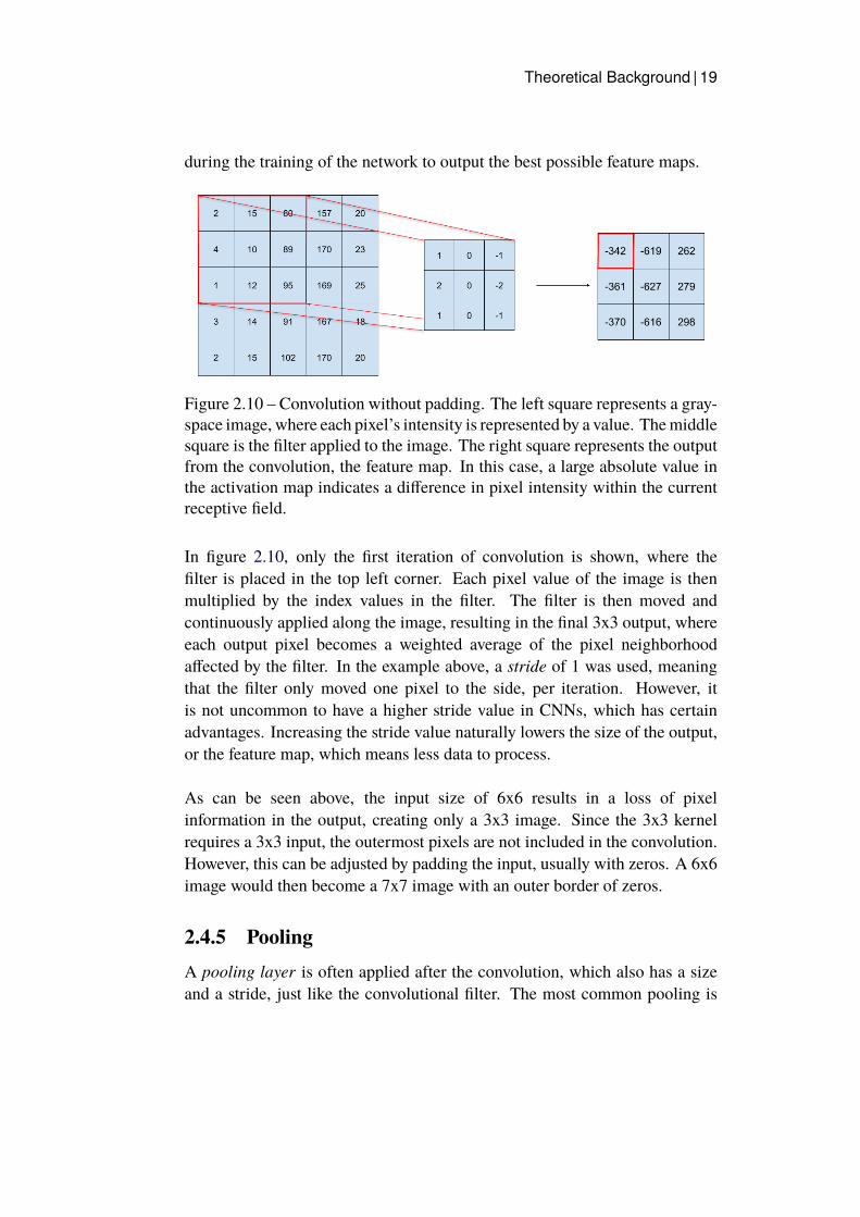
Figure 2.10 – Convolution without padding. The left square represents a gray-space image, where each pixel’s intensity is represented by a value. Themiddlesquare is the filter applied to the image. The right square represents the outputfrom the convolution, the feature map. In this case, a large absolute value inthe activation map indicates a difference in pixel intensity within the currentreceptive field.

In figure 2.10, only the first iteration of convolution is shown, where thefilter is placed in the top left corner. Each pixel value of the image is thenmultiplied by the index values in the filter. The filter is then moved andcontinuously applied along the image, resulting in the final 3x3 output, whereeach output pixel becomes a weighted average of the pixel neighborhoodaffected by the filter. In the example above, a stride of 1 was used, meaningthat the filter only moved one pixel to the side, per iteration. However, itis not uncommon to have a higher stride value in CNNs, which has certainadvantages. Increasing the stride value naturally lowers the size of the output,or the feature map, which means less data to process.

As can be seen above, the input size of 6x6 results in a loss of pixelinformation in the output, creating only a 3x3 image. Since the 3x3 kernelrequires a 3x3 input, the outermost pixels are not included in the convolution.However, this can be adjusted by padding the input, usually with zeros. A 6x6image would then become a 7x7 image with an outer border of zeros.

2.4.5 PoolingA pooling layer is often applied after the convolution, which also has a sizeand a stride, just like the convolutional filter. The most common pooling is


max-pooling, which takes the max value of the area of interest in the featuremap and stores only that. Figure 2.11 shows an example of max-pooling, usinga size of 2 and a stride of 1, which is applied to the convolution result.

Figure 2.11 – An example of max-pooling. From each resulting neighborhoodof pixels, the largest pixel value is chosen. The size of the neighborhooddepends on the size of the max-pooling. Here, a 2x2 max-pooling is shown.

Pooling is not required in a CNN, but it achieves not only a smallerrepresentation of the data, but also introduces some translation invariance tothe system. A translation shift in the input does not necessarily lead to a greatchange in the output, since pooling does not consider the absolute locations ofpixels but rather individual neighborhoods.

2.4.6 Related WorkThe study is motivated by papers written on non-DL methods used forparameter extraction of FMCW and Polyphase signals [6], [7], [8] [22].These studies used the Wigner-Wille Distribution to generate TF-images,followed by either only a Hough transform or a combination of a Hough andRadon transform, to extract parameters.

The methodology used is based on the regular discrete WVD, whichcreates their image of interest. The WVD is followed by a Hough transform, amethod that has been used for a long time in computer vision to detect edgesand irregularities in images. The Hough transform takes an image, specificallypixels of high intensity, from Cartesian space into Hough space. In Houghspace, lines are no longer expressed by their Cartesian representation

y = a ∗ x+ b (2.13)


where a is the slope of the line and b is the point of intersection with the y-axis. Instead, they are expressed through variables θ and ρ [23]. The Houghtransform assumes that pixels that stand out from the rest in intensity, mayrepresent a line. So, for each pixel, if the intensity value is greater than acertain threshold, the following equation is applied

ρ = x ∗ cos(θ) + y ∗ sin(θ) (2.14)

where (x, y) represents the pixel location in the image and ρ is the magnitudeof a vector that goes from (0, 0) to the closest point on the potential line thatgoes through (x, y). The angle of this vector is given by θ and is the anglebetween the x-axis and the vector. Since all that is known about the pixel is thatit has an intensity that was higher than a set threshold, no information aboutthe angle of the line can be known. Therefore, the above equation is usuallyapplied for every θ = 1...180. For each (ρ, θ) pair, a zero-initialized matrix isincremented by 1 in each [ρ, θ] index. Pixels that form a line return the sameρ value for the same θ values and therefore increment the [ρ, θ] index in thematrix. After passing through all the pixels in the image, the (ρ, θ) indices inthematrix with the highest numbers will represent the lines found in the image.

With the image taken into Hough space and the [ρ, θ] indices with thehighest values found, the distance between the two lines is calculated. In [6],[23], [23] [22], their method requires at least two chirps in the same TF-image.With this requirement, both the modulation time and the bandwidth can becalculated through the use of θ, which is the same for both chirps in the image.

These are autonomous algorithms that rely on other methodologies thanmachine learning and deep learning. These methods show high accuracy, butat low noise levels. At high noise levels, the results become less reliable. Thisis because they always assume that the most intense point in Hough/Hough-Radon-space is the active signal. Through this assumption, they can acquirethe signal’s carrier frequency, which is a valid method at low noise levels butnot with increasing noise.

These techniques mostly produce precise and consistent results; however, theyare unreliable in their carrier frequency estimation in noisier environments.Outside of parameter estimation, there has been a significant amount of workon DL and LPI over the past years. In 2016, Zhang et al. presented a solutionfor autonomous LPI radar recognition, managing to classify 8 different


modulations at a 94.7% accuracy at a Signal-to-Noise Ratio (SNR) level of-2 dB [24]. They did not, however, employ a CNN, but rather a variant of anRNN (Recurrent Neural Network) called an Elman network. Despite usingan RNN, they still created images using the Choi-Williams Distribution butthen manually extracted features from them, before feeding the data into theElman network.

An article released in 2018 by Limin and Xin [25] was more in linewith the approach taken in this report, utilizing a modified AlexNet [26] andthe SPWVD to classify LPI modulations. In addition, they applied their ownmodifications to AlexNet, managing to decrease the number of parametersfrom 55M to 39M, while claiming to maintain the same performance. In theirreport, a total of ten different LPI modulations were used, and at an SNR levelof -6 dB, they achieved a 92.5% overall accuracy for all classes.

In 2019, Hoang et al. [27] combined classification, parameter extraction andDeep Learning. However, despite utilizing DL for their classification task,they did not do so for their parameter estimation. In the study, they considered12 LPI modulations and utilized the networks SSD (Single-Shot multi-boxDetector) and YOLOv3 (You Only Look Once), for their classificationtask. When determining parameters of signals, they borrowed the methodsdescribed in [22] and [6] to extract values for polyphase and FMCW signals.However, they proposed their own solution to extracting parameters fromCostas signals.

Even though their method of classification utilizes DL, their parameterextraction does not. From a generated TF-image of the Costas sequence, theyuse computer vision methods such as global thresholding and openings andclosings to reduce noise and make the signal more clear. They also use asegmentation algorithm to find the centers of the Costas steps and calculateparameters such as sequence length and time for each step. Their methodis deemed reliable to an SNR level of -2 dB. However, they do not presentresults clearly for the Costas parameters, which makes it difficult to makedirect comparisons. Since they also did not publish results for SNR levelsless than -4 dB, a comparison to their performance can not be made in thisthesis, which looks at lower SNR levels.

Methodology | 23

Chapter 3

Methodology

This chapter explains what methods and architectures were used to acquireresults and how they were evaluated. The chapter starts with data generation,building upon the background on In-phase and Quadrature (IQ)-data andLPI-modulations presented in chapter 2. Then, information on the machinelearning methodologies used in this thesis is presented, together with theneural network architectures used. Finally, the tests conducted in this thesisare given, along with metrics taken during the tests to determine theirperformance.

3.1 Data generationAcquiring recorded LPI radar is difficult, especially for data sets as large asthose needed for the training of ANNs. Data may be classified, or simply notexist in the easily acquirable form required for this kind of work. Because ofthis, only artificial data was used in this work. How data was generated foreach signal is described in the subsections below. All signals went throughthe same preprocessing that took place before using the SPWVD to creategray-space images.

The first step of preprocessing was the addition of Additive white Gaussiannoise (AWGN) to the signal. AWGN is commonly used to replicate therandomness that can be found in nature, and represents the electromagneticnoise that LPI signals use to remain undetected. The networks weretrained on SNR levels from -1 dB to -10 dB. The noise ratios were chosenbased on previous works that have conducted experiments in similar noiseenvironments [6, 8, 7, 25]. Equation 3.1 shows that at SNR = 0 dB, the

24 | Methodology

power ratio is equal to 1, i.e. the signal and the noise have the same power.While at SNR = −10 dB, the power of the noise is ten times that of thesignal.

SNRdB = 10 ∗ log10(PsignalPnoise

) (3.1)

After adding noise, slicing of the signal was done to add further randomnessto the look of the signals. As a result of generating signals artificially, themodulation always started in the first recorded sample, a scenario that isunrealistic in actual LPI recordings. Therefore, 2048 samples were initiallygenerated, and then cut down to 1024, through a random selection ofconsecutive samples. This final, processed, IQ-data was then fed into theSPWVD-function, to create 128x128 gray-space images.

3.2 Signals & ParametersIn this study, three LPI signal types were analyzed, Frank and Costas signals,as well as the common FMCW modulation. All signals had an amplitude of1 and were sampled with a sampling rate of fs = 8000Hz. The followingsubsections introduce the parameters that were estimated, what ranges theywere generated within and how the signals were produced.

3.2.1 FMCWFor every FMCW signal, the variables in table 3.1 were randomized withinthe ranges presented.

Table 3.1 – FMCWParameters that were estimated. f0 is the carrier frequency,∆f is the bandwidth andmt is the modulation time.

Parameters f0 (kHz) ∆f (kHz) mt (ms)Range 1 - 2 0.5 - 1.5 20 - 80Method Regression Regression Regression

The FMCW signal can take on three different modulation forms, chirp-up,chirp-down or triangle formation, which is why the generation of IQ pairshas different definitions depending on modulation type. A sequence of IQvalues for chirp-up is given by equation 3.2, chirp-down by equation 3.3 and

Methodology | 25

the triangle modulation by their modified combination.

upI = A ∗ cos(2π ∗ ((f0 +∆f

2) · t− ∆f

mt· t2))

upQ = A ∗ sin(2π ∗ ((f0 +∆f

2) · t− ∆f

mt· t2))

(3.2)

downI = A ∗ cos(2π ∗ ((f0 −∆f

2) · t+

∆f

mt· t2))

downQ = A ∗ sin(2π ∗ ((f0 −∆f

2) · t+

∆f

mt· t2))

(3.3)

The triangle modulation is generated just as above, but the modulation timefor the up-chirp and down-chirp is halved, and then they are sampled one afteranother. This way, half the modulation time is spent increasing the frequency,while the other half is spent decreasing, or vice versa.

For eqs. (3.2) and (3.3), ∆f represents the bandwidth of the FMWCsignal, i.e. how wide the frequency change is. f0 is the carrier frequencyand mt represents the modulation time expressed in milliseconds. The aboveexpressions are defined for t = [0,mt], and then extend with a period ofmt.

3.2.2 Frank CodeAll signals were randomized within the ranges presented in 3.2, and thenestimated in the testing of the network’s performance.

Table 3.2 – Frank parameters that were estimated. f0 is the carrier frequency,CPP is the cycles per phase and N is the number of phases.

Parameters f0 (kHz) CPP NRange 1 - 2 1 - 10 1 - 10Method Regression Classification Classification

The generation of the Frank signals was also done through calculations ofIQ-pairs. For every increase in i, the phase jumps are increased by 2 ∗ π

N

and for every j, a phase shift of the current size, given by the current i, istaken. For each i and j, equation 3.4 was used to generate IQ-pairs, where0 < n < ceil(fs

f) ∗ CPP and tb = 1

fs. This means that a higher CPP leads

to a longer stay on the same phase and more IQ-pairs generated for the samei and j. Equation 3.4 shows how the IQ-pairs were generated, where ωc is the

26 | Methodology

carrier frequency and the remaining variables are defined as explained above.

I = A ∗ cos(ωc(n− 1) ∗ tb+ φi,j)

Q = A ∗ sin(ωc(n− 1) ∗ tb+ φi,j)(3.4)

For the Frank signals, carrier frequencywas estimated, just like for the FMCW,in order to determine whether outputting one variable instead of three mighthave an impact on performance. The variables that were estimated throughclassification in the Frank signals were CPP , or cycles per phase, and thenumber of code phases, N . Again, a higher CPP means that the signal willstay on the same phase for longer, for multiple cycles. The number of codephases is the variable N described above. It controls the size of the Frankmatrix that makes up all the phase shifts, the larger the number of code phases,the smaller the phase shifts.

3.2.3 Costas CodeThe estimated Costas parameters were randomized for each signal within theranges shown in 3.3.

Table 3.3 – Costas Parameters that were estimated. Ff is the first frequencystep, ∆f is the bandwidth and sl is the sequence length.

Parameters Ff (kHz) ∆f (kHz) slRange 0.275 - 6 0.15 - 3.5 3 - 8Method Regression Regression Classification

Complete parameter estimation of a Costas sequence is not a trivial task. So,instead of training multiple networks for each Costas length, a few parametersthat could show if parameter estimation is possible for Costas, were chosen.These are bandwidth (∆f ), sequence length (sl), and the frequency of thefirst step (Ff ) in the Costas sequence.

The bandwidth, ∆f , of a Costas sequence is defined as the differencebetween the highest frequency step and the lowest frequency step. Togetherwith the bandwidth, the frequency of the first step, Ff , of the sequence wasestimated. Like with FMCW, these are two continuous parameters, and weretherefore estimated in the same network and the same forward pass.

Lastly, the sequence length was estimated through classification. However,

Methodology | 27

this classification task is not as straightforward as it may seem. Due to thestructure of Costas arrays, the number of valid configurations rises, up to apoint, as the sequence length grows. Generating based on the occurrencesof each sequence length could therefore result in an imbalanced data set.However, for this thesis, an equally distributed data set was generated instead.With all lengths being equally represented in the data set, it is important tobear in mind that the shorter sequences look more similar to one another thanthe longer ones. Since there are only three Costas sequence patterns to choosefrom, of length 3, they might end up looking very similar.

First, a random length between 3 and 8 was chosen, and a random sequenceof that length was selected. The sequence, consisting of values representingthe y-axis index in the Costas array, was then turned into a sequence offrequencies within the desired range, through the expression in 3.5.

seq = seq ∗ randint(75, 500) + randint(200, 2000) (3.5)

The time between each frequency hop was also randomized, according toexpression 3.6.

tp = 10−2 ∗ (rand(0, 1) ∗ 1.4 + 0.6) (3.6)

After setting the frequencies and time period for each sequence, the IQpairs could then be generated similarly to the other signals described earlier.Equation 3.7 shows the IQ sampling, where seq(x) is the frequency of thecurrent index as 0 < x < len(seq), tb = 1

fsand n controls the length of each

frequency step by depending on tp.

I = A ∗ cos(2 ∗ π ∗ seq(x) ∗ (n− 1) ∗ tb)Q = A ∗ sin(2 ∗ π ∗ seq(x) ∗ (n− 1) ∗ tb) (3.7)

3.3 ImplementationTwo different machine learning approaches have been combined for theproblem of parameter estimation. The first approach is more commonly usedfor continuous output, and it is regression. Since continuous values representsome of the parameters of interest i.e. bandwidth or carrier frequency, bothexpressed in continuous Hz, a regression model makes a lot of sense. Inregression, the relationship between a dependent variable and one or moreindependent variables is mapped. In a neural network setting, the network

28 | Methodology

weights and biases are fitted to best approximate the output.

The second approach is classification where the model learns to categorizeinput data into one of the multiple classes. Traditionally, classification hasbeen used to differentiate between classes that take on distinctly differentfeatures, which is not necessarily the case for this thesis. The parametersestimated through classification are integer values being estimated, and notdistinctly different classes. From that perspective, classification may notbe the optimal way of determining these parameters. Nonetheless, for thisproject, multi-class classification was used to categorize input signals intodiscrete categories.

3.3.1 ArchitecturesFive architectures were implemented to provide comparisons betweennetwork size, estimation performance, and inference time. A larger networkwill probably take longer to produce results, but the results may be ofhigher quality. The largest archtiectures are based on the VGG architecturespresented in [28]. Figure 3.1 illustrates the layout of the largest neural networkused. Observe that for each network, batch norm and pooling were usedbetween every layer, except between Conv3 and Conv4 and between Conv5and Conv6. This design choice was made to match the design of VGGNetbetter. Also, for the classification tasks, the final layer has softmax applied toit.

In tables 3.4 to 3.8 the architectures used for the project are presented.Different output sizes, stride lengths and paddings have been used to create arange of network sizes.

Methodology | 29

Table 3.4 – CNN0 - 76 million parameters

Layer Kernel Input size Output size Stride Activation PaddingConv1 3x3 1x128x128 64 1 LeakyReLU ZerosConv2 3x3 64x64x64 128 1 LeakyReLU ZerosConv3 3x3 128x32x32 256 1 LeakyReLU ZerosConv4 3x3 256x32x32 256 1 LeakyReLU ZerosConv5 3x3 256x16x16 512 1 LeakyReLU ZerosConv6 3x3 512x16x16 512 1 LeakyReLU ZerosDense1 - 512x8x8 2048 - LeakyReLU -Dense2 - 2048 1024 - LeakyReLU -Dense3 - 1024 256 - LeakyReLU -Dense4 - 256 noutputs - - -


Layer Kernel Input size Output size Stride Activation PaddingConv1 3x3 1x128x128 64 1 LeakyReLU -Conv2 3x3 64x64x63 128 1 LeakyReLU -Conv3 3x3 128x30x30 256 1 LeakyReLU -Conv4 3x3 256x28x28 256 1 LeakyReLU -Conv5 3x3 256x13x13 512 1 LeakyReLU -Conv6 3x3 512x11x11 512 1 LeakyReLU -Dense1 3x3 512x4x4 2048 1 LeakyReLU -Dense2 - 2048 1024 - LeakyReLU -Dense3 - 1024 256 - LeakyReLU -Dense4 - 256 noutputs - - -


Layer Kernel Input size Output size Stride Activation PaddingConv 3x3 1x1x128 64 1 LeakyReLU -Conv 3x3 64x42x42 256 1 LeakyReLU -Conv 3x3 256x11x11 256 1 LeakyReLU -Conv 3x3 256x3x3 256 1 LeakyReLU -Dense - 256x3x3 1024 - LeakyReLU -Dense - 1024 256 - LeakyReLU -Dense - 256 noutputs - - -

30 | Methodology

Table 3.7 – CNN3 - 960k parameters

Layer Kernel Input size Output size Stride Activation PaddingConv 7x7 1x128 64 2 LeakyReLU -Conv 3x3 64x30x30 128 2 LeakyReLU -Conv 3x3 128x7x7 256 2 LeakyReLU -Conv 3x3 256x3x3 256 2 LeakyReLU -Dense - 256 noutputs - - -

Table 3.8 – CNN4 - 242k parameters

Layer Kernel Input size Output size Stride Activation PaddingConv 7x7 1x1x128 32 2 LeakyReLU -Conv 3x3 32x30x30 64 2 LeakyReLU -Conv 3x3 64x7x7 128 2 LeakyReLU -Conv 3x3 128x3x3 128 2 LeakyReLU -Dense - 128 noutputs - - -

64 128

128

conv1

128 112

conv2

256 256 56

conv3-4

512 512 28

conv5-61 20

48

fc1

1 1024

fc2

1 256

fc3

Figure 3.1 – The largest network is shown, where the yellow and orange layersrepresent the Convolutional layers and the LeakyReLU activation. The smallerred layers that follow are the result of Max-pooling. The purple layers are thefully connected layers that create the final output value. Depending on theapplication, the last layer may have a softmax activation or create multipleoutputs. Here, the final output size is not shown.

Methodology | 31

3.3.2 SetupAll models were trained with the Adam optimizer, using an initial learningrate of 0.0001. The β values were maintained at their default values ofβ1 = 0.9 and β2 = 0.999, and so was the error term ε = 1e − 8. Thesevalues were chosen since they were the recommended hyperparameter valuesin the original publication on Adam in 2015 [29]. Because of the limitationson time and resources, no hyperparameter search was made. The trainingcontinued until ten epochs had passed without a decrease in validation loss,and the model from the training epoch with the lowest validation loss wasthen kept for future testing. This ensured that the networks reached theirbest possible weight configurations without being limited by the number oftraining epochs.

Further, the same seed was used for the shuffling of training data toensure the data order did not affect the training results. Following bestpractices, the regression variables were normalized within the range [0,1] and so were the pixel intensities in the images. All architectures wereimplemented using Python 3.6.8, and Pytorch 1.8.1, early stopping based onvalidation loss was accomplished through the use of Pytorch Lightning 1.2.4.The IQ-samples were generated using Matlab scripts and the TF-images weregenerated using the Matlab WVD-function. The experiments were executedon a desktop with an Intel i9-9900 CPU @3.1GHz and an Nvidia RTX 2080SUPER GPU with 8GB VRAM.

3.4 EvaluationCommonly used metrics have been implemented and recorded to monitor theperformance of a network’s predictions during tests, both for the regressiveparameters and for those determined through classification. The followingsection describes these metrics.

3.4.1 RegressionThere are many ways to assess the performance of a regression model, butthey all have their basis in calculating the difference between the network’sestimation and the ground truth.

32 | Methodology

Error distribution & Mean

A basic evaluation metric of regression estimates is the mean error, theaverage difference between the correct answer and the estimation provided bythe network. This metric can show if the network is skewed in its predictions,overshooting or undershooting correct answers, but the mean error does notsay much more than that. If the network tends to undershoot, the mean errorwill be a negative value, if it overshoots, it will be a positive value. However,if the network equally undershoots and overshoots, the mean error will becentered around zero, which is preferable.

A better indicator for actual performance is the standard deviation ofthe errors. The greater the error of the estimations, the greater the standarddeviation of the network’s predictions. Two networks with error meanscentered around zero may still have very different standard deviations.Naturally, a network with a smaller deviation of errors is a better predictor.

Mean Squared Error

The MSE was the loss function used during the training of all regressionnetworks. Since it was used to train the networks, it is also valuable to testthe networks on it, to understand how well the network adapts to unseen data.The MSE is given by equation 3.8.

MSE =1

n

n∑i=1

(Yi − Yi)2 (3.8)

where Yi is the observed value and Yi is the predicted value. The MSEalways returns a positive value and provides a useful metric to compare theperformance of the networks. However, it can be skewed by outliers becauseof the squared error.

Mean Absolute Error & Max Absolute Error

An alternative to the MSE is the Mean Absolute Error, which computes theabsolute value of the errors, instead of squaring them. This means that outliersdo not affect the calculations as heavily as they do when using the MSE.

MAE =1

n

n∑i=1

(|Yi − Yi|) (3.9)

Methodology | 33

In addition to the MAE, the Maximum Absolute Error was used as well. TheMaximumAbsolute Error was the only metric that provided information aboutthe actual largest errors, which could be a useful metric to analyze whenconsidering the worst case performance.

Akaike Information Criterion

The Akaike Information Criterion (AIC) was introduced by Akaike in 1974[30], and is often used to compare and choose between nonlinear regressivemodels [31]. It is an alternative to the R2 metric often used to compare linearregression models. The AIC penalizes regressive models by their size andassumes that too complex models will overfit. The metric was not originallydesigned for neural networks, and the assumption that ANNs suffer fromoverfitting is debatable, see for example this online discussion by BradyNeal 1. From the perspective of overfitting for neural networks, the AIC maytherefore not be the most optimal metric.

However, since the size of each architecture is assumed to correlate toinference time, the AIC score may then become a combined metric ofestimation performance and inference time. What the AIC provides is not ascore that necessarily says anything about the accuracy of the model itself, butrather provides a score that allows for models to be compared to one another.A lower score means that the model is a better choice, according to the AIC.

Since Least Squares estimation was used, a special case of the AIC canbe used for the score calculation [32]:

AIC = n ∗ log(σ2) + 2K (3.10)

σ2 =∑

(ε2

n) (3.11)

where n is sample size, K is the number of parameters in the model and εrepresents the estimation errors. A modified version of the AIC, the AICc, isshown in equation 3.12 and it takes into account small sample sizes comparedto a large number of parameters, and should always be used unless n

K> 40.

AICc = AIC +2K(K + 1)

n−K − 1(3.12)

1 https://www.bradyneal.com/bias-variance-tradeoff-textbooks-update

34 | Methodology

Note that as n → ∞ then the AICc → AIC. Since the AIC values presentno information about the absolute performance, the values can be normalizedso that the lowest value is fixed to 0 and the largest to 1, as shown in eq. 3.13.

AICnorm =AIC − AICmaxAICmax − AICmin

(3.13)

3.4.2 ClassificationThe performance of a classification model does not only depend on theclassification accuracy, i.e., the ratio between correct predictions and totalpredictions. Depending on the data, the total classification accuracy may notcapture all the information of the results. For this reason, Precision and Recallhave been used as additional metrics.

Accuracy

For the five architectures defined, five models of each were trained, with thebest performing model selected for presentation of results. The selection ofthe best model was based on overall accuracy across all classes. This wascalculated as shown below in equation 3.14.

Accuracy =

∑nc=1(TPc)∑n

c=1(TPc+FPc+FNc)

nclasses(3.14)

Precision & Recall

After selecting the best model, based on overall accuracy, the Precision andthe Recall were the two performance metrics used to evaluate the models anddisplay their performance.

The precision for each class in a multi-class problem is calculated asshown in equation 3.15.

Precisionc =(TPc)

(TPc + FPc)(3.15)

where TPc is the number of true positives for each class c i.e. the examplesthat were correctly predicted to belong to class c, and FPc is the numberof false positives for each class c, i.e. all examples that were incorrectlypredicted to belong to class c.

Methodology | 35

The recall for each class in a multi-class problem is defined in equation3.16.

Recallc =(TPc)

(TPc + FNc)(3.16)

where TPc is the number of true positives for each class c and TNc isthe number of false negatives for each class c, i.e. all examples that wereincorrectly predicted example not to belong to class c.

A macro score for both the precision and the recall was calculated aswell, showing the performance averaged over all classes. These are definedin 3.17 and 3.18, and use the score from each individual class to calculate amacro score.

Recallmacro =

∑nc=1(Recallc)

nclasses(3.17)

Precisionmacro =

∑nc=1(Precisionc)

nclasses(3.18)

3.5 TestingThe following section describes the tests conducted and how they relate to theformulated research question and its sub-questions.

3.5.1 Estimation accuracy - Primary testA test for accuracy over a range of SNR levels was defined to answer the firstresearch sub-question. For this test, 50000 images were generated for eachmodulation type, ranging in SNR from -1 dB to -10 dB. For each modulation,the images were then split into two sets, training, and testing, with a train/testsplit of 0.9/0.1, which consisted of a random selection of images from eachSNR level. The training set, consisting of 45000 images per modulation, wasfurther divided into training/validation sets with another 0.1/0.9 split. Thevalidation set of 4500 images was used to monitor the model’s performanceand halt training once the validation loss stopped decreasing. For all primarytests, five variants of each architecture were trained. This was done tominimize the risk of poor random initialization and to monitor how much theresults fluctuate between identical nets.

Once training was finalized, testing with the test set was conducted.

36 | Methodology

The best performing network from the five models was then selected to beused for the remaining evaluation metrics. Which network actually performedthe best was established through the comparison of Mean Squared Error inthe case of regression and overall accuracy for classification.

3.5.2 Speed & Throughput - Secondary testIn order for CNNs to be a viable option for radar systems, not only theiraccuracy has to be high, but so does their speed. Dummy data was createdthrough the random initialization of images, to measure the networks’inference times. These images were then passed through the models, withvarying batch sizes in the range [1, 64]. For each size, 300 iterations were runon each model for each batch size, from which the minimum value was beselected. The minimum value provides the most valuable information sincethe time can increase slightly between runs for various reasons, but it cannever be lower than its lowest possible time.

From the inference time, the maximum throughput of the models canbe calculated. Inverting the inference time and multiplying with the batchsize provides the maximum number of images per second.

Results | 37

Chapter 4

Results

This chapter presents the results of the primary and secondary tests. Theresult presentation follows the formulation of the research sub-questions byfirst presenting the performance of the networks in the primary test and thenpresenting the throughput of the networks in the secondary test.

4.1 Primary testThe primary test measured performance of the networks using the metricsdescribed in chapter 3. The results are presented in modulation order, startingwith FMCW, then Frank, and finally Costas signals. For the primary test, fivemodels of each architecture were tested, and the results achieved by the bestnetworks are presented. For the regression variables, the model selection isbased on the lowest MSE value, and for classification variables, models arechosen based on overall accuracy.

4.1.1 FMWCBelow follow the tables and graphs from the FMCW parameter estimations.All parameters were estimated through regression. Since five models of eacharchitecture was trained, the best one was selected for further testing, based onthe minimum mean squared error (MSE). The model that produced the bestMSE values across both the model variation and the primary tests are shownin bold text in the tables.

38 | Results

Model variation

ThemeanMSE for all models and FMCWvariables is displayed in 4.1. CNN0achieves the smallest MSE and the smallest 95% confidence interval across allvariables. Performance then decreases with network size. From all models,the network with the lowest MSE had its performance measured fully in theprimary test.

CNN f0 ∆f mt

0 0.0036 ± 2.5e-04 0.0031 ± 2.3e-04 0.0022 ± 6.7e-051 0.0055 ± 9.4e-04 0.0058 ± 1.7e-03 0.0040 ± 1.2e-032 0.0072 ± 1.1e-03 0.0086 ± 1.9e-03 0.0062 ± 1.0e-033 0.0174 ± 2.1e-03 0.0230 ± 3.6e-03 0.0216 ± 2.8e-034 0.0157 ± 2.3e-03 0.0222 ± 4.4e-03 0.0212 ± 3.7e-03

Table 4.1 – The mean MSE and the 95% confidence interval for FMCWparameters f0, ∆f andmt, for five trained models and across all architectures.

Performance

All architectures had their best performing model selected and that model’sresults presented in the following section. Figure 4.1 shows the drop-off inregression performance with a decrease in network size and the higher peaksachieved by CNN0. From figure 4.1, it can also be seen that the smallernetworks, CNN3 and CNN4, sometimes do not manage to center their errorsaround 0 and instead over- or undershoot.

Results | 39

Figure 4.1 – The results for FMCW estimations displayed as normaldistributions, calculated from the mean and the standard deviation of eachvariable. The y-axes show the density of probability and the x-axes show theestimation error. The results are from the models that were chosen based ontheir MSE result. The leftmost image shows results for f0, the middle for ∆f ,and the right formt.

The tables 4.2 to 4.4 show the metrics, with CNN0 outperforming the othernetworks across all metrics but Max Error. The standard deviation shows thatabout 68% of estimations are at less than a 6% error and 95% are at less thana 12% error, for CNN0. Further, it is also shown that CNN4 consistentlymanages to perform better than CNN3 across all metrics, resulting in a lowerAIC score.

CNN MEAN STD MSE MAE Max Error AIC

0 0.0032 0.0587 0.0035 0.0315 0.7725 0.00001 -0.0012 0.0685 0.0047 0.0384 0.7554 0.20732 0.0038 0.0792 0.0063 0.0478 0.6238 0.40043 0.0202 0.1229 0.0155 0.0898 0.7065 1.00004 -0.0289 0.1084 0.0126 0.0788 0.6141 0.8390

Table 4.2 – f0 - Carrier frequency metrics.


0 0.0044 0.0544 0.0030 0.0319 0.4890 0.00001 0.0050 0.0665 0.0045 0.0394 0.6002 0.21032 -0.0060 0.0860 0.0074 0.0553 0.6752 0.47613 -0.0171 0.1420 0.0204 0.1088 0.6284 1.00004 0.0026 0.1274 0.0162 0.0937 0.6027 0.8634

Table 4.3 – ∆f - Bandwidth metrics.

40 | Results


0 0.0012 0.0465 0.0022 0.0255 0.6470 0.00001 -0.0061 0.0587 0.0035 0.0331 0.6049 0.22322 0.0102 0.0734 0.0055 0.0445 0.6403 0.43653 0.0026 0.1357 0.0184 0.0983 0.9019 1.00004 -0.0224 0.1294 0.0173 0.0957 0.7598 0.9546

Table 4.4 –mt - Modulation time metrics.

4.1.2 Frank CodeFor Frank modulations, carrier frequency (f0) was estimated throughregression, while cycles per phase (CPP ) and the number of code phases(N ) were estimated through classification. The best performing networks areshown in bold text, based on the MSE for regression variables and maximumaccuracy for the classification variables.

Model variation - f0

For Frank signals, f0 was estimated through regression, and again five modelsof each network were trained, with the best version being chosen based onthe lowest MSE value. Table 4.6 shows the MSE variation within the fivemodels that were trained for each network. The MSE dropped consistentlywith network size, and the performance remained relatively stable across thedifferent models.

CNN f0

0 0.0019 ± 5.7e-051 0.0022 ± 1.4e-042 0.0027 ± 3.1e-043 0.0037 ± 1.4e-044 0.0036 ± 3.3e-04

Table 4.5 – The mean MSE and the 95% confidence interval for Frankparameter f0 over five trained models and across all architectures.

Results | 41

Performance

Figure 4.2 – A normal distribution plot of the estimation error of Frank signals’carrier frequency, f0. The y-axis shows the density of probability and thex-axis shows the estimation error. The figure shows the results for the bestperforming models across all architectures.

Across all architectures and for the selectedmodels, themetrics STD,MSE andMAE all consistently show smaller values than they did for f0 estimation inFMCW. These results also show that CNN1 is closer in performance to CNN0than for the FMCWparameters. Further, the smallest network now achieves anMSE that is almost identical to what CNN0 achieved for the estimation of f0in FMCW. Nonetheless, with a standard deviation of 0.0431 for CNN0, about68% of results lie within a 4% error, and 95% within a 9% error.


0 0.0028 0.0431 0.0019 0.0240 0.5245 0.00001 0.0014 0.0449 0.0020 0.0267 0.3451 0.12542 0.0033 0.0498 0.0025 0.0307 0.3788 0.44453 -0.0037 0.0598 0.0036 0.0405 0.5312 1.00004 0.0056 0.0581 0.0034 0.0400 0.4950 0.8714

Table 4.6 – Carrier frequency - f0 metrics for Frank signals.

42 | Results

Model variation - CPP

The variation between each model is displayed in table 4.7, where thedifference betweenmodels is shown to be the largest for CNN4. The differencein accuracy between the best- and the worst performing model for CNN4 isabout 25 percentage points. From the results in table 4.7, the best performingnetwork was selected based on maximum accuracy across all classes.

CNN Min Max Mean

0 0.710 0.758 0.737 ± 2.6e-021 0.595 0.618 0.609 ± 1.1e-022 0.587 0.607 0.593 ± 1.1e-023 0.525 0.545 0.536 ± 1.1e-024 0.219 0.473 0.316 ± 1.2e-01

Table 4.7 – The Min, Max and Mean accuracy with the 95% confidenceinterval for CPP , over five trained models across all architectures.

Performance

The macro values for the CPP estimation are given in table 4.8, whichshows a decrease in both recall and precision with network size. The recalland precision values are almost identical for all networks, except for CNN4,which nearly achieves the same precision as CNN3, but falls behind furtherin the recall.

The figs. 4.3 and 4.4 show that CNN0 achieves the highest precisionand recall across most CPP values, as well as the most consistency. Thesmaller networks, CNN3 and CNN4 perform well for some values, but showpoor performance across others.

Results | 43

CNN Recall Precision

0 0.7542 0.76291 0.6154 0.61522 0.6031 0.61403 0.5418 0.54504 0.4722 0.5347

Table 4.8 – Themacro recall and precision forCPP estimation. The presentedresults were achieved by the best performing models from each architecture.

Figure 4.3 – The recall achieved by the best performing models for differentCPP values.

Figure 4.4 – The precision achieved by the best performingmodels for differentCPP values.

44 | Results

Model variation - N

The table 4.9 shows the results for the different models of each network size.There is a distinct jump in performance fromCNN0 to the rest of the networks;also CNN2 seems to outperform CNN1 across most models, showing a smallvalue for the standard error of the mean.

CNN Min Max Mean

0 0.611 0.667 0.632 ± 2.8e-021 0.389 0.448 0.416 ± 3.6e-022 0.431 0.449 0.439 ± 1.1e-023 0.372 0.401 0.392 ± 1.5e-024 0.367 0.417 0.401 ± 2.6e-02

Table 4.9 – The Min, Max and Mean accuracy with the 95% confidenceinterval for code phase estimation over five trained models across allarchitectures.

Performance

Table 4.10 shows the macro values for recall and precision, and a drop inperformance from CNN0 to CNN1, but then consistent macro performanceas network size continues to decrease. In figs. 4.5 and 4.6, the indicatedperformance difference from table 4.10 is shown across different phase values.The precision for CNN0 is higher across all code phase values, but has adistinct drop in performance at N = 5, a pattern that is not as distinct for therest of the networks. Also, the recall for CNN0 is the highest across all phases,but the performance difference is not as high as for the precision. There is alsoa pattern of decreasing recall with a higher number of phases, for all networks.

Results | 45


0 0.6622 0.67521 0.4434 0.43302 0.4444 0.44193 0.3970 0.38874 0.4120 0.4035

Table 4.10 – The macro recall and precision for code phase estimation. Thepresented results were achieved by the best performing models from eacharchitecture.

Figure 4.5 – The recall achieved by the best performing models for differentnumber of code phases.

Figure 4.6 – The precision achieved by the best performingmodels for differentnumber of code phases.

46 | Results

4.1.3 Costas CodeFor the Costas modulation, the first frequency (Ff ) and the bandwidth(∆f ) were estimated through regression, while the sequence length (sl) wasestimated through classification. The network that produces the lowest MSEis shown in bold text for the regression variables, and the network withthe highest maximum accuracy is shown in bold text for the classificationvariables.

Model variation - Ff ∆f

The variation between versions of the networks is shown in table 4.11.The MSE values show that the performance difference between networksfor estimation of Ff is small. Estimating ∆f , however, shows decreasingperformance with network size.

CNN Ff ∆f

0 0.0102± 9.3e-04 0.0050 ± 1.7e-031 0.0107 ± 9.4e-04 0.0072 ± 2.6e-032 0.0114 ± 4.4e-04 0.0096 ± 1.7e-043 0.0117 ± 1.2e-04 0.0115 ± 7.5e-044 0.0111 ± 2.7e-04 0.0109 ± 5.1e-04

Table 4.11 – The mean MSE and the 95% confidence interval for Costasparameters Ff , and ∆f for five trained models and across all architectures.

Performance

Figure 4.7 and table 4.12 show that predicting the first frequency of theCostas sequence can not be done accurately and the distribution of errors iswide for all networks. There is also no real performance difference betweeneach network, as shown in table 4.12 where most metrics are similar for allnetworks. Bandwidth, however, seems to behave similarly to the bandwidthestimation of FMCW, where performance drops with network size. Table 4.13shows this behavior and also indicates that it can be done to a similar errorperformance to that of FMCW, despite the range of the bandwidth being largerthan that of FMCW signals.

Results | 47

Figure 4.7 – Normal distributions of of errors for Ff and ∆f estimation inCostas signals. The y-axes show the density of probability and the x-axes showthe estimation error. The figures show results achieved by the best performingmodel from each architecture.


0 0.0030 0.0988 0.0098 0.0708 0.5491 0.00001 0.0014 0.1015 0.0103 0.0716 0.7015 0.33252 -0.0024 0.1048 0.0110 0.0773 0.5530 0.70723 -0.0118 0.1071 0.0116 0.0806 0.6061 1.00004 -0.0096 0.1041 0.0109 0.0774 0.5671 0.4341

Table 4.12 – Ff metrics for Costas signals.


0 0.0057 0.0645 0.0042 0.0392 0.6764 0.00001 -0.0002 0.0782 0.0061 0.0481 0.7778 0.41172 -0.0007 0.0968 0.0094 0.0712 0.6754 0.87643 0.0049 0.1027 0.0106 0.0751 0.7125 1.00004 -0.0220 0.0987 0.0102 0.0744 0.6419 0.9281

Table 4.13 – ∆f metrics for Costas signals.

Classification - sl

Again, the selection of each network was conducted through a comparisonof accuracy. The results from Costas sequence length through classification

48 | Results

are presented in table 4.1.3. There is a drop in accuracy from CNN0 to theother networks, but there is also a much greater spread amongst the modelsfor CNN0, as indicated by the SEM value.

CNN Min Max Mean

0 0.425 0.568 0.537 ± 7.8e-021 0.274 0.295 0.283 ± 1.0e-022 0.306 0.334 0.315 ± 1.5e-023 0.270 0.280 0.274 ± 4.7e-034 0.248 0.307 0.267 ± 2.8e-02

Table 4.14 – The Min, Max and Mean accuracy with the 95% confidenceinterval for sl over five trained models across all architectures.

Performance

The figs. 4.8 and 4.9 and table 4.15 display the results achieved by thenetworks. The table shows a drop in performance across both metrics fromCNN0 to CNN1, but then consistent macro values with decreasing parametercount. Figure 4.8 shows how all networks perform similarly across lengths 3,7, and 8, but that CNN0 achieves much higher recall across the other lengths.For the precision shown in 4.9, CNN0 achieves nearly twice the performanceacross most lengths.


0 0.5710 0.57001 0.2959 0.28142 0.3347 0.32903 0.2810 0.26554 0.3091 0.2849

Table 4.15 – The macro recall and precision for sl estimation. The presentedresults were achieved by the best performing models from each architecture.

Results | 49

Figure 4.8 – The recall achieved by the best performing models for slestimation.

Figure 4.9 – The precision achieved by the best performing models for slestimation.

4.2 Secondary test - Speed and ThroughputFirst of all, every network was tested on the same hardware, as defined insection 3.3.2. The tables 4.16 and 4.17 and figs. 4.10 and 4.11 show arelationship between model size and inference time. The smaller models havea constant inference time for a while as the batch size grows, while the largermodels show an immediate increase in inference time. At batch size = 64,the throughput that CNN4 achieves is over 20 times that of CNN0, bearing inmind though that the number of parameters in CNN0 is over 300 times that ofCNN4.

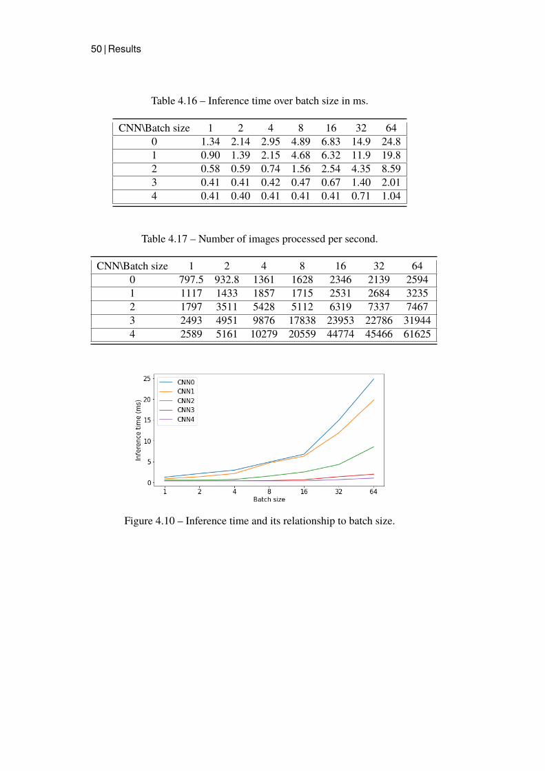
50 | Results

Table 4.16 – Inference time over batch size in ms.

CNN\Batch size 1 2 4 8 16 32 640 1.34 2.14 2.95 4.89 6.83 14.9 24.81 0.90 1.39 2.15 4.68 6.32 11.9 19.82 0.58 0.59 0.74 1.56 2.54 4.35 8.593 0.41 0.41 0.42 0.47 0.67 1.40 2.014 0.41 0.40 0.41 0.41 0.41 0.71 1.04

Table 4.17 – Number of images processed per second.

CNN\Batch size 1 2 4 8 16 32 640 797.5 932.8 1361 1628 2346 2139 25941 1117 1433 1857 1715 2531 2684 32352 1797 3511 5428 5112 6319 7337 74673 2493 4951 9876 17838 23953 22786 319444 2589 5161 10279 20559 44774 45466 61625

Figure 4.10 – Inference time and its relationship to batch size.

Results | 51

Figure 4.11 – Throughput and its relationship to batch size.

52 | Results

Discussion | 53

Chapter 5

Discussion

5.1 Primary testsParameter estimation is possible with DL on the synthetic data used in thisthesis. Except for estimating the first frequency in a Costas sequence, allregression variables showed a maximum standard deviation of roughly 0.065,for CNN0. This means that 68% of all test samples lie within a 6.5% error,and 95% lie within a 13% estimation error. These are good results, but, asalways, even better results can likely be achieved with more training data.

5.1.1 FMCWComparing FMCW performance to the numbers presented by Gulum et al. in[7], a publication that presents numbers for three SNR levels, [3, -3, -9] dB,gives some indication on how well the networks perform. Creating standarddeviation representation of the results achieved for FMCW signals in [7], thestandard deviations across SNR levels can be summarized as:

SNR f0 ∆f mt

3 dB 0.0306 0.0151 0.0058-3 dB 0.0847 0.0200 0.005-9 dB 1.1951 0.0352 0.0156

Table 5.1 – Standard deviation of variables from [7].

The results for ∆f and mt are strong across all SNR levels, bearing in mind,however, that the tests in [7] only consist of 9 signals per SNR level. Theestimation for f0 suffers a lot when the noise gets too strong, and the techniques

54 | Discussion

can not reliably estimate the carrier frequency at all, something a DL approachdoes not suffer from. The results are comparable to the ones achieved for mostregression parameters in this thesis. This does not only include FMCW butFrank and even Costas bandwidth as well, which had a much wider range thanthe other parameters.

5.1.2 FrankAs shown in section 4.1.2, estimating f0 could be done more accurately forFrank signals than for FMCW signals, despite their identical ranges. Thismay be because the networks only had to adapt to one parameter insteadof three. It also allowed the smaller networks to perform better, probablybecause they did not have to capture a wider set of patterns.

The classification results also indicate that the patterns can be captured,at least by the largest network. For CPP estimation, classification accuracydropped as the network size decreased. Compared to the other parameterestimated by classification, CPP followed the decrease in network sizemore linearly. Estimating the number of code phases, N , gave interestingresults, where there was a distinctive jump in precision at N = 5 for CNN0.There was also a general decrease in both recall and precision as the numberof phases increased, for all networks. It could be that the signals becomeincreasingly similar as the number of phases grows, and are not discerniblydifferent from one another.

5.1.3 CostasLooking at the estimation of the length of the Costas sequence, performancedid not drop with network size except for the initial drop from CNN0 toCNN1. It may just be that these patterns are too difficult for smaller networksto capture, and they manage to learn whatever brings the lowest validationloss. From the precision and recall figures, it becomes clear that no networkbut CNN0 captured the patterns across all sequence lengths. This outcomemay also be a result of the iteration selection based on the highest overallaccuracy. Perhaps the networks with the highest accuracy were the onesthat predicted either length 3 or 8, and the ones that tried to capture a moreadvanced pattern did not manage to reach a high enough accuracy to beselected.

Discussion | 55

5.1.4 AICA discussion on the AIC metric is necessary, since it did not provide theinformation expected. The AIC score always followed the results acquiredfrom the MSE, i.e., giving the best result to the net with the smallest MSE.This is due to the AIC penalty term, which is supposed to discourage the useof too large models, not being large enough in comparison to the residual sumof square errors. It is not unreasonable to think that the AIC score should favorsmaller models for the estimation of Ff in Costas signals. The performancedifference between networks was minimal, but the best AIC value was stillgiven to CNN0, the largest model.

5.2 Secondary tests - Speed and throughputWhen it comes to speed and throughout, the smallest network, CNN4,achieved upwards of 61000 images per second. With a single imageconsisting of 1024 samples, this equates to about 60 million samples persecond, or a possible sampling rate of 60MHz, without information loss inreal-time. The largest network, CNN0, achieved only about 2600 imagesper second, which means a possible sampling rate of about 2.6MHz. Theresults show that throughput increases with batch size, which is also expectedwith GPUs, since memory transfers greatly impact their performance. Usinga GPU with more memory would allow for a larger batch, and thereforeincreased performance. Another way of achieving higher throughput is bysampling for longer. Creating images of 2048 samples instead of 1024 leadsto the same inference time in the network, but twice the samples analyzed.The downside to this strategy is the time spent waiting for more information;gathering more samples means that the response will be slower. It is importantto bear in mind that a non-negligible time is also spent creating the WVDimages, a time measurement that is not included here but one that must beconsidered for future viability tests.

Expectedly, the networks can not support the high sampling rate ofradar systems if they must process every sample. However, in applicationswhere the processing of each sample is not required, the methodology used inthis thesis may still be viable.

56 | Discussion

5.3 Advantages & DisadvantagesThe greatest benefit the ANNs in this thesis can provide, compared to themethods presented in section 2.4.6, is another level of automation andpotentially speed. Although hardware dependent, creating Hough/Hough-Radon images will always be an intermediary step not necessary in the DLsolution presented here. Furthermore, no fine tuning of thresholds is requiredto find the relevant pixels; everything is sorted by the ANNs. Not only isno thresholding necessary, essentially no work is required to fit the modelsto any parameter and signal of interest, which is not the case for the earliermentioned models. Also, the methods presented in 2.4.6 place requirementson there being at least two active signals within the created image, which isnot needed in the proposed DL solution. Finally, even though the networksperform worse as SNR goes down, they never become completely unreliable.This was an issue in [7, 8] , where carrier frequency estimation becamealmost impossible.

However, an ANN solution has its drawbacks as well. The methodswill always produce estimations. Two signals with the same bandwidth butwith different carrier frequencies would probably not get the same bandwidthreturned from the networks, since their images would be different. They alsohave to be trained on a specific data set, set in a particular environment, adrawback that is not found in traditional, trigonometry-based methods.

5.4 Future WorkThe work and results presented clearly show that the extraction of parametersis possible through CNNs operating on TF-images created using the WVD.However, there are other routes that can be explored as well.

Through the WVD, there is some information loss, going from IQ datato a TF image. This is, of course, not optimal, and could be avoided throughwork done on IQ data. It would then perhaps also be possible to make moreaccurate predictions over time through the use of Recurrent Neural Networksor similar architectures such as Gated Recurrent Unit or Long Short-TermMemory nets. These network architectures can maintain context and thereforeanalyze longer sequences of data such as speech or text. It might be possibleto use them in the context of radar analysis and parameter extraction, insteadof operating on TF-images, and some work has been done on radar, using

Discussion | 57

these techniques [33] [34].

More work also needs to be done with broader parameter and SNRranges. What ranges can the networks be trained on and still reach acceptableresults? At what point in SNR do the networks stop working reliably?The more diverse the data, the more difficult the networks will be to train.Further, what happens to the accuracy when the sampling rate is increased toreasonable radar levels? No radar today operates at the sampling rate used inthis thesis, and is not representative of a real electromagnetic environment. Itis, therefore, possible that the look of the WVD images may be different atreal sampling rates, perhaps hurting performance.

When it comes to potentially improving the estimation performance ofthe networks, it is clear that a substantial increase in parameters from CNN1to CNN0, and perhaps the use of padding lead to a performance difference.Creating even larger networks may be a simple way of improving performance,but with the drawback of slower inference time. Another approach may be thatof Ensemble Learning [35], simply the training and use of multiple iterationsof the same network. Since networks are commonly randomly initialized, theconvergence between identical networks may still differ greatly. Combiningmultiple networks may therefore improve generalization performance. This,of course, places heavy requirements on GPU performance, memory andbandwidth, if multiple models are to be run in parallel, without an increase ininference time.

5.5 Ethical & Societal aspectsSaab is a company that produces and sells equipment within the defenseand civil industry, a practice that comes with its own questions regardingethics. The Just war theory states that war may be morally justifiable throughcertain criteria, which are summarized as Jus ad bellum - the right to go towar, and Jus in bello - right conduct within war [36]. This essentially statesthat war, sometimes, is the best cause of action when the other options areeven more terrible. However, one must make a personal stance regarding thedevelopment of technologies used within the defense industry, and there iscertainly a case to be made for the opposition of research and developmentwithin the defense sector. One ethical issue arises from one of Saab’s largestcustomers, the Swedish Defence Materiel Administration (FMV). This is a

58 | Discussion

government agency operating under the Swedish ministry of defense, whichin turn means that Saab is partly funded by taxpayers, to develop materielused in warfare. The implications are that, essentially, no one in Sweden candistance themselves financially from the investment into war materiel, whichmay not line up with everyone’s ethics.

This project has only looked at possible changes and developments toradar receivers at a very basic level. The individual technology itself cannot directly cause harm to others as it is more likely to possible serve inRadar Warning Receivers or the likes to keep people alive. Nonetheless, it ispossible that they, as an indirect consequence, can be used to enable harm,especially in the wrong hands. Because of this, Saab follows strict policiesregarding sustainability, anti-corruption, system safety, etc, to ensure it meetsthe ethical standards set by the industry.

5.6 SustainabilityThe possible sustainability aspects of DL have become a reality over the pastfew years. See for example this discussion 1 where papers such as [37] ismentioned, a study in which they found that the training of a large NaturalLanguage Processing (NLP) DL model could lead to emissions of 620 000CO2e. As the models grow in size and complexity, training and computetimes grow with it. The largest DL model, released in 2020 [38], has 175billion trainable parameters, making it the largest model by a factor 10,compared to the second-largest Microsoft’s Turing NLG 2. Microsoft’s modelwas released only a few months before GPT-3, and the rapid growth withinDL models may very well continue in the coming years.

However, DL may have another effect on sustainability. A study released inearly 2020 [39], concluded that of all the Sustainable Development Goals andtargets defined by Unicef 3, Artificial Intelligence (AI) could aid in reaching134, or 79% of these. Worth mentioning, however, is that AI might also havea negative impact on a total of 59 targets or 35%. The targets were dividedinto societal, economical, and environmental targets, where environmentaltargets turned out to possibly benefit the most from AI.1 https://news.mit.edu/2020/shrinking-deep-learning-carbon-footprint-08072 https://www.microsoft.com/en-us/research/blog/turing-nlg-a-17-billion-parameter-language-model-by-microsoft/ 3 https://sdgs.un.org/goals

Discussion | 59

Nevertheless, the direct impact this work may have on sustainability isthe generalized platform that DL offers. Working on General ProcessingUnits instead of hardware specifically designed for a certain task will probablyaffect the sustainability of Saab’s development. Creating a wide variety ofsoftware solutions on one common hardware platform may massively lowerthe production costs, and with it, production emissions.

60 | Discussion

Conclusions | 61

Chapter 6

Conclusions

This study has investigated the viability of utilizing CNNs, the SPWVD andTF-images to estimate the parameters of LPI radar modulations. It has beenshown that parameter estimation is possible with DL on most parameters usedin this thesis. Additionally, the speed of the networks has been analyzed andshown to not be high enough to process every sample in radar systems, withoutinformation loss. However, the inference times may be satisfactory for use inother applications that do not require analysis of every sample. Furthermore,there are methods to improve both estimation performance and throughputperformance, some of which have been discussed. More work within lowerSNR levels, broader parameter ranges, and tests that more closely simulatean electromagnetic environment that a radar receiver might actually perceive,would be natural future work. Much continued work is required to fullydetermine the viability of DL models within LPI radar parameter estimation.

62 | Conclusions

REFERENCES | 63

References

[1] S. S. Swords, Technical History of the Beginnings of Radar. IET, Jan.1986. [Online]. Available: https://doi.org/10.1049/pbht006e

[2] A. Bole, A. Wall, and A. Norris, “Chapter 1 - basic radar principles,”in Radar and ARPA Manual (Third Edition), third edition ed., A. Bole,A. Wall, and A. Norris, Eds. Oxford: Butterworth-Heinemann,2014, pp. 1 – 28. ISBN 978-0-08-097752-2. [Online]. Available: http://www.sciencedirect.com/science/article/pii/B9780080977522000015

[3] O. Russakovsky, J. Deng, H. Su, J. Krause, S. Satheesh, S. Ma, Z. Huang,A. Karpathy, A. Khosla, M. Bernstein, A. C. Berg, and L. Fei-Fei,“ImageNet Large Scale Visual Recognition Challenge,” InternationalJournal of Computer Vision (IJCV), vol. 115, no. 3, pp. 211–252, 2015.doi: 10.1007/s11263-015-0816-y

[4] F. Sultana, A. Sufian, and P. Dutta, “Evolution of image segmentationusing deep convolutional neural network: A survey,” CoRR, vol.abs/2001.04074, 2020. [Online]. Available: https://arxiv.org/abs/2001.04074

[5] Z. Zhao, P. Zheng, S. Xu, and X. Wu, “Object detection with deeplearning: A review,” CoRR, vol. abs/1807.05511, 2018. [Online].Available: http://arxiv.org/abs/1807.05511

[6] T. Gulum, A. Erdogan, T. Yildirim, and L. Durak Ata, “Parameterextraction of fmcw modulated radar signals using wigner-houghtransform,” in 12th IEEE International Symposium on ComputationalIntelligence and Informatics, CINTI 2011 - Proceedings, 11 2011. doi:10.1109/CINTI.2011.6108551 pp. 465–468.

[7] T. O. Gulum, A. Y. Erdogan, T. Yildirim, and P. E. Pace, “Aparameter extraction technique for fmcw radar signals using wigner-

https://doi.org/10.1049/pbht006e

http://www.sciencedirect.com/science/article/pii/B9780080977522000015

http://www.sciencedirect.com/science/article/pii/B9780080977522000015

https://arxiv.org/abs/2001.04074


http://arxiv.org/abs/1807.05511

64 | REFERENCES

hough-radon transform,” in 2012 IEEE Radar Conference, 2012. doi:10.1109/RADAR.2012.6212255 pp. 0847–0852.

[8] K. K. Guner, T. O. Gulum, and B. Erkmen, “Fpga-based wigner–houghtransform system for detection and parameter extraction of lpiradar lfmcw signals,” IEEE Transactions on Instrumentation andMeasurement, vol. 70, pp. 1–15, 2021. doi: 10.1109/TIM.2021.3060584

[9] A. Wulff, Beginning radio communications : radio projects and theory.New York: Apress, 2019. ISBN 978-1-4842-5302-1

[10] Z. Khatib, Distributed CMOS bidirectional amplifiers : broadbandingand linearization techniques. New York, NY: Springer, 2012. ISBN978-1-4614-0272-5

[11] A. T. Poyil and N. KM, “Study on performance of wigner villedistribution for linear fm and transient signal analysis,” InternationalJournal of Electronics and Communication Engineering, vol. 6, no. 8,pp. 877 – 880, 2012. [Online]. Available: https://publications.waset.org/vol/68

[12] “Wigner-ville distribution and smoothed pseudo wigner-villedistribution,” https://se.mathworks.com/help/signal/ref/wvd.html,accessed: 2021-05-17.

[13] P. Pace, Detecting and classifying low probability of intercept radar.Boston: Artech House, 2009. ISBN 9781596932340

[14] R. Frank, “Polyphase codes with good nonperiodic correlationproperties,” IEEE Transactions on Information Theory, vol. 9, no. 1, pp.43–45, 1963. doi: 10.1109/TIT.1963.1057798

[15] J. Costas, “A study of a class of detection waveforms having nearly idealrange—doppler ambiguity properties,” Proceedings of the IEEE, vol. 72,no. 8, pp. 996–1009, 1984. doi: 10.1109/PROC.1984.12967

[16] K. Drakakis, “Open problems in Costas arrays,” Tech. Rep., Mar 2011,comments: 24 pages. [Online]. Available: http://cds.cern.ch/record/1332993

[17] W. S. McCulloch andW. Pitts, “A logical calculus of the ideas immanentin nervous activity,” The bulletin of mathematical biophysics, vol. 5,no. 4, pp. 115–133, 1943.

https://publications.waset.org/vol/68

https://publications.waset.org/vol/68

https://se.mathworks.com/help/signal/ref/wvd.html

http://cds.cern.ch/record/1332993

http://cds.cern.ch/record/1332993

REFERENCES | 65

[18] A. L. Maas, A. Y. Hannun, and A. Y. Ng, “Rectifier nonlinearitiesimprove neural network acoustic models,” in in ICMLWorkshop onDeepLearning for Audio, Speech and Language Processing, 2013.

[19] I. Goodfellow, Y. Bengio, and A. Courville,Deep Learning. MIT Press,2016, http://www.deeplearningbook.org.

[20] K. Fukushima, “Neocognitron: A self-organizing neural network modelfor a mechanism of pattern recognition unaffected by shift in position,”Biological Cybernetics, vol. 36, pp. 193–202, 1980.

[21] D. H. Hubel and T. N. Wiesel, “Receptive fields of single neurones inthe cat’s striate cortex,” The Journal of Physiology, vol. 148, no. 3, pp.574–591, 1959. doi: https://doi.org/10.1113/jphysiol.1959.sp006308.[Online]. Available: https://physoc.onlinelibrary.wiley.com/doi/abs/10.1113/jphysiol.1959.sp006308

[22] T. Gulum, P. Pace, and R. Cristi, “Extraction of polyphase radarmodulation parameters using a wigner-ville distribution - radontransform,” in 2008 IEEE International Conference on Acoustics, Speechand Signal Processing, 05 2008. doi: 10.1109/ICASSP.2008.4517907pp. 1505 – 1508.

[23] R. O. Duda and P. E. Hart, “Use of the hough transformation todetect lines and curves in pictures,” Commun. ACM, vol. 15, no. 1, p.11–15, Jan. 1972. doi: 10.1145/361237.361242. [Online]. Available:https://doi-org.focus.lib.kth.se/10.1145/361237.361242

[24] M. Zhang, L. Liu, and M. Diao, “Lpi radar waveform recognitionbased on time-frequency distribution,” Sensors, vol. 16, no. 10, 2016.doi: 10.3390/s16101682. [Online]. Available: https://www.mdpi.com/1424-8220/16/10/1682

[25] G. Limin and C. Xin, “Low probability of intercept radarsignal recognition based on the improved alexnet model,” inProceedings of the 2nd International Conference on Digital SignalProcessing, ser. ICDSP 2018. New York, NY, USA: Associationfor Computing Machinery, 2018. doi: 10.1145/3193025.3193037.ISBN 9781450364027 p. 119–124. [Online]. Available: https://doi.org/10.1145/3193025.3193037

http://www.deeplearningbook.org

https://physoc.onlinelibrary.wiley.com/doi/abs/10.1113/jphysiol.1959.sp006308

https://physoc.onlinelibrary.wiley.com/doi/abs/10.1113/jphysiol.1959.sp006308

https://doi-org.focus.lib.kth.se/10.1145/361237.361242

https://www.mdpi.com/1424-8220/16/10/1682

https://www.mdpi.com/1424-8220/16/10/1682

https://doi.org/10.1145/3193025.3193037

https://doi.org/10.1145/3193025.3193037

66 | REFERENCES

[26] A. Krizhevsky, I. Sutskever, and G. Hinton, “Imagenet classification withdeep convolutional neural networks,” Neural Information ProcessingSystems, vol. 25, 01 2012. doi: 10.1145/3065386

[27] L. M. Hoang, M. J. Kim, and S. . Kong, “Deep learning approach to lpiradar recognition,” in 2019 IEEE Radar Conference (RadarConf), 2019.doi: 10.1109/RADAR.2019.8835772 pp. 1–8.

[28] K. Simonyan and A. Zisserman, “Very deep convolutional networksfor large-scale image recognition,” in 3rd International Conference onLearning Representations, ICLR 2015, San Diego, CA, USA, May 7-9,2015, Conference Track Proceedings, Y. Bengio and Y. LeCun, Eds.,2015. [Online]. Available: http://arxiv.org/abs/1409.1556

[29] D. P. Kingma and J. Ba, “Adam: A method for stochastic optimization,”in 3rd International Conference on Learning Representations, ICLR2015, San Diego, CA, USA, May 7-9, 2015, Conference TrackProceedings, Y. Bengio and Y. LeCun, Eds., 2015. [Online]. Available:http://arxiv.org/abs/1412.6980

[30] H. Akaike, “A new look at the statistical model identification,” IEEETransactions on Automatic Control, vol. 19, no. 6, pp. 716–723, 1974.doi: 10.1109/TAC.1974.1100705

[31] A.-N. Spiess and N. Neumeyer, “An evaluation of r2 as an inadequatemeasure for nonlinear models in pharmacological and biochemicalresearch: a monte carlo approach,” BMC Pharmacology, vol. 10,no. 1, Jun. 2010. doi: 10.1186/1471-2210-10-6. [Online]. Available:https://doi.org/10.1186/1471-2210-10-6

[32] K. P. Burnham and D. R. Anderson, “Multimodel inference,”Sociological Methods & Research, vol. 33, no. 2, pp. 261–304,Nov. 2004. doi: 10.1177/0049124104268644. [Online]. Available:https://doi.org/10.1177/0049124104268644

[33] V. Jithesh, M. J. Sagayaraj, and K. G. Srinivasa, “Lstm recurrentneural networks for high resolution range profile based radartarget classification,” in 2017 3rd International Conference onComputational Intelligence Communication Technology (CICT), 2017.doi: 10.1109/CIACT.2017.7977298 pp. 1–6.



https://doi.org/10.1186/1471-2210-10-6

https://doi.org/10.1177/0049124104268644

REFERENCES | 67

[34] D. Roy, S. Srivastava, A. Kusupati, P. Jain, M. Varma, andA. Arora, “One size does not fit all: Multi-scale, cascaded rnns forradar classification,” in Proceedings of the 6th ACM InternationalConference on Systems for Energy-Efficient Buildings, Cities, andTransportation, ser. BuildSys ’19. New York, NY, USA: Associationfor Computing Machinery, 2019. doi: 10.1145/3360322.3360860. ISBN9781450370059 p. 1–10. [Online]. Available: https://doi.org/10.1145/3360322.3360860

[35] M. A. Ganaie, M. Hu, M. Tanveer, and P. N. Suganthan, “Ensembledeep learning: A review,” CoRR, vol. abs/2104.02395, 2021. [Online].Available: https://arxiv.org/abs/2104.02395

[36] A. Lang, Just war : authority, tradition, and practice. Washington, DC:Georgetown University Press, 2013. ISBN 978-1-58901-996-6

[37] E. Strubell, A. Ganesh, and A. McCallum, “Energy and policyconsiderations for deep learning in NLP,” CoRR, vol. abs/1906.02243,2019. [Online]. Available: http://arxiv.org/abs/1906.02243

[38] T. B. Brown, B. Mann, N. Ryder, M. Subbiah, J. Kaplan, P. Dhariwal,A. Neelakantan, P. Shyam, G. Sastry, A. Askell, S. Agarwal, A. Herbert-Voss, G. Krueger, T. Henighan, R. Child, A. Ramesh, D. M. Ziegler,J. Wu, C. Winter, C. Hesse, M. Chen, E. Sigler, M. Litwin, S. Gray,B. Chess, J. Clark, C. Berner, S. McCandlish, A. Radford, I. Sutskever,and D. Amodei, “Language models are few-shot learners,” 2020.

[39] R. Vinuesa, H. Azizpour, I. Leite, M. Balaam, V. Dignum, S. Domisch,A. Felländer, S. D. Langhans, M. Tegmark, and F. Fuso Nerini, “The roleof artificial intelligence in achieving the sustainable development goals,”Nature communications, vol. 11, no. 1, pp. 233–233, 2020.

https://doi.org/10.1145/3360322.3360860

https://doi.org/10.1145/3360322.3360860



www.kth.se

TRITA -EECS-EX-2021:715

Parameter Estimation of LPI Radar in Noisy Environments ...

Documents

Transcript of Parameter Estimation of LPI Radar in Noisy Environments ...