
Nonlinear dynamical analysis of noisy time series
61
Penultimate Draft of a paper in press in Nonlinear Dynamics in Psychology and the Life Sciences, 2005 1 Nonlinear dynamical analysis of noisy time series. Andrew Heathcote & David Elliott School of Behavioural Sciences The University of Newcastle Australia RUNNING HEAD: Analysis of chaos in noise Correspondence should be addressed to : Andrew Heathcote, Aviation Building, The University of Newcastle, University Drive, Callaghan, 2308, NSW, Australia. Email: [email protected] Phone: 61-2-49215952 Fax: 61-2-49216906
Transcript of Nonlinear dynamical analysis of noisy time series

Penultimate Draft of a paper in press in Nonlinear Dynamics in Psychology and the Life Sciences, 2005
1
Nonlinear dynamical analysis
of noisy time series.
Andrew Heathcote & David Elliott
School of Behavioural Sciences
The University of Newcastle
Australia
RUNNING HEAD: Analysis of chaos in noise
Correspondence should be addressed to: Andrew Heathcote, Aviation Building, The
University of Newcastle, University Drive, Callaghan, 2308, NSW, Australia.
Email: [email protected] Phone: 61-2-49215952 Fax: 61-2-49216906
Penultimate Draft of a paper in press in Nonlinear Dynamics in Psychology and the Life Sciences, 2005
2
Empirical time series in the life sciences are often non-stationary and have small signal-
to-noise ratios, making it difficult to accurately detect and characterize dynamical
structure. The usual response to high noise is averaging, but time domain averaging is
inappropriate, especially when the dynamics are nonlinear. We review alternative delay-
space averaging methods based on the topology and short-term predictability of nonlinear
dynamics and illustrate their application using the TISEAN software (Hegger, Kantz &
Schreiber, 1999). The methods were applied to a Lorenz series, which resembles the
dynamics found by Kelly, Heathcote, Heath and Longstaff (2001) in series of decision
times. The Lorenz series was corrupted with up to 80% additive Gaussian noise, a lower
signal-to-noise ratio than has been used in any previous test of these methods, but
consistent with Kelly et al.’s data. Prediction methods performed the best for detecting
nonstationarity and nonlinear dynamics, and optimal predictability provided an objective
criterion for setting the parameters required by the analyses. Local linear filtering
methods preformed best for characterization, producing informative plots that revealed
the nature of the underlying dynamics. These results suggest that a methodology based on
delay-space averaging and prediction could be useful with noisy empirical data series.
Keywords: Nonlinear Dynamics, Fractal Dimension, Prediction, Time Series,
Measurement Noise

Penultimate Draft of a paper in press in Nonlinear Dynamics in Psychology and the Life Sciences, 2005
3
The study of mathematical chaos has provided useful new techniques for the
analysis of time series (e.g., Hegger, Kantz & Schreiber, 1999) and a framework for
models of complex behavioural processes (e.g., Gregson, 1988, 1992, 1995; Guastello,
1995; Heath, 2000; Kelso, 1995; Newell, Liu & Mayer-Kress, 2001). However, most of
these techniques were developed for the physical sciences where the underlying
determining equations are usually known and measurement noise can be minimised. In
the behavioural sciences, in contrast, determining equations are rarely known, and it is
difficult to eliminate measurement noise because measured systems cannot be sufficiently
isolated to remove the effects of influential environmental variables.
This paper addresses the application of nonlinear dynamical analysis (NDA)
techniques to behavioural data with particular reference to the problem of measurement
noise. The usual response to noise in the behavioural sciences is averaging. However,
when behaviour is nonlinear, inappropriate averaging can introduce distortion so that the
average is not representative of any individual’s behaviour (e.g., Brown & Heathcote,
2003; Heathcote & Brown, 2004; Heathcote, Brown & Mewhort, 2000). Once the
necessity of studying the individual is accepted, one is faced with a daunting level of
variability in behaviour. Gilden (1997), for example, found that changes in the mean
accounted for only 10% of individual variance in a range of choice response time (RT)
experiments. Discarding the remaining 90% of variation as “error” assumes that no
systematic explanation is possible for the vast majority of individual behaviour.
Nonlinear dynamics, which can generate complex and apparently random behaviour
while obeying relatively simple deterministic equations, provides an alternative
conceptualisation of behavioural variability. As Luce (1995) states: “… the findings of
Penultimate Draft of a paper in press in Nonlinear Dynamics in Psychology and the Life Sciences, 2005
4
the past 10 to 15 years about nonlinear dynamic systems call into question whether the
actual source of the noise is randomness or ill-understood dynamics.” (p.24).
However, it is unlikely that chaotic dynamics can explain all of the variability of
individual behaviour. The research reported here was inspired by studies of sequential
dependences in the times to make series of simple choices, which under the right
conditions can show evidence for nonlinear dynamics (Kelly, Heathcote, Heath &
Longstaff, 2001), but also clearly contained high levels of measurement noise. Where
genuine noise is present, measurement of dynamics becomes problematic.
Nonlinear Dynamics
Figure.1a is an example of low-dimensional mathematical chaos, a time series
from the Lorenz equations (see caption for details), which will be used to illustrate
nonlinear dynamics throughout this paper. The Lorenz series was chosen because its
dynamics resemble those observed by Kelly et al. (2001). The Lorenz series exhibits a
pair of complex oscillatory states, with rapid transitions between these states occurring at
apparently irregular intervals. Within each state, oscillations increase from small to large
amplitudes before undergoing a state transition. The series in Fig.1a begins with a rapid
state transition then spends a long time in the lower state, but later in the series the upper
state has the majority of extended oscillations. The first major section of this paper
reviews a range of NDA techniques and applies them to the Lorenz series. We then
examine NDA for noisy series of the type that might be expected in behavioural data, by
adding Gaussian noise to the series in Fig.1a.
-------------------------------- Insert Figure 1 about here
---------------------------------

Penultimate Draft of a paper in press in Nonlinear Dynamics in Psychology and the Life Sciences, 2005
5
It should be emphasised from the outset that is difficult to provide a definitive
step-by-step guide that covers NDA for all types of nonlinear dynamics. The very
complexity that makes nonlinear dynamics attractive for modelling also means that
caution is required in generalising findings about a particular type of chaotic series.
Rather, the aim of this paper is to illustrate an investigative methodology that readers can
adapt in order to ascertain if NDA will be useful with their own data, perhaps aided by
analysis of model time series. The analysis software used here (with commands set in
Courier) is available free through the TISEAN project (Version 2.1,
http://www.mpipks-dresden.mpg.de/~tisean, see Hegger, Kantz & Schreiber, 1999).
Methods for Dynamical Analysis
Chaos can range from low dimensional to high dimensional. Although noise and
high dimensional chaos are conceptually distinct, they are almost impossible to
distinguish in practice. Low dimensional chaos can be distinguished from noise, but
obtaining data of sufficient quality can be difficult. The time series must be long, sampled
at regular time intervals, and stationary (stationarity is defined below). Initially, NDA
techniques were developed for physical science applications that yielded such series. In
the life sciences, however, long stationary series are difficult to obtain, due to processes
such as learning and fatigue, and high levels of measurement noise are often present.
Genuine noise, particularly linearly autocorrelated noise, is problematic as it can appear
like chaos to some NDA techniques.
The Fourier power spectrum of the series in Fig.1a illustrates why noise is
problematic for NDA. Fourier analysis is a traditional approach to such apparently
structured oscillatory signals, allowing for dominant frequencies to be identified through
peaks in the spectrum, and broadband noise to be removed through band-pass filtering.

Penultimate Draft of a paper in press in Nonlinear Dynamics in Psychology and the Life Sciences, 2005
6
However chaotic signals can themselves be broadband, and so frequency domain filters
are ineffective. Where noise is white (i.e., each sample is independent) the spectrum is
flat. Coloured noises, such as are produced by linear and nonlinear autocorrelation
produce spectra, are characterised by a decrease in power with increasing frequency. The
Lorenz series also displays a decrease in power as frequency increases. The similarity of
spectra for chaos and coloured noises makes them hard to distinguish.
Whereas Fourier decomposition transforms temporal informa tion into frequency
information, most NDA techniques rely on the transformation of temporal information
into a geometrical representation: delay embedding. An m dimensional delay embedding
converts a one dimensional time series, x(t), to a set of m dimensional points (x(t+δ),
x(t+2δ),…x(t+mδ)), where δ is the time delay between samples. Takens’ (1981) theorem
states that a one to one image of the d dimensional set of points visited by a stationary
dynamical system (its attractor) can be reconstructed from an embedding in a delay space
with dimension m>2d. For the Lorenz system, for example, d≈2.05, with the attractor
being a fractal subset of the space defined by the three Lorenz variables (i.e., (x,y,z) of
which only x is shown in Fig.1a). The complex, fractal nature of this set for chaotic
systems have led to them being described as “strange attractors”. Since Takens’ initial
result, “embedology” has been an active area of theoretical development, with Sauer,
Yorke and Casdagli (1991) showing that more general schemes than simple delay
coordinates can be used, including delay embeddings of series transformed by singular
value decomposition and geometric filtering (Grassberger, Hegger, Kantz, Schaffrath &
Schreiber, 1993).

Penultimate Draft of a paper in press in Nonlinear Dynamics in Psychology and the Life Sciences, 2005
7
Stationarity is essential for establishing an embedding. For a stochastic process,
y(t), stationarity can be defined as invariance of all finite-dimensional joint distribution
functions of (y(t1),y(t2),…y(tm)) over shifts on the temporal dimension (e.g., (t1+∆…tm+∆))
(Rao & Gabr, 1984). In the context of NDA, Casdagli (1997, p. 12) stated that for
practical purposes: “…a time series x1, x2,…,xN is nonstationary if, for low m, there are
variations in the estimated joint distribution of xi,xi+1,…,xi+m-1 that occur on time scales of
order N”. An embedded representation can only translate all temporal information to
spatial information if the underlying process is stationary. Given stationarity, NDA can
recover aspects of the dynamics using geometrical analyses of the embedded set. The
analyses often involve estimating the properties of local neighbourhoods or sets of points,
with a neighbourhood defined on a distance measure in the embedding space. Where such
analyses aggregate local measures to estimate global properties of the attractor they
strongly rely on the assumption of stationarity. Aggregation is particularly important to
counter the effects of measurement noise.
Even where stationarity holds, it should be acknowledged that a particular data
series may not be suitable for NDA if all regions of the dynamics are not sampled, and
hence the full joint distribution cannot be estimated. As in conventional statistics, one
needs a sufficient number of replicates to form a reliable model, so intermittent chaos or
noisy periodic behaviours cannot be characterized when few intermittent events or
periods are sampled. In some circumstances, even arbitrarily small amounts of noise can
destroy the embedding property (Casdagli, Eubank, Farmer & Gibson, 1991). However,
delay coordinates are also useful when an embedding is not required, such as in the
prediction of nonlinear time series with both deterministic and stochastic dynamical
Penultimate Draft of a paper in press in Nonlinear Dynamics in Psychology and the Life Sciences, 2005
8
structure (Weigend & Gershenfeld, 1993). As will be discussed later, NDA based on
prediction is especially attractive because it remains useful when noise levels are high.
Figure 2a illustrates the nonlinear dynamics of the Lorenz time series, by plotting
each value against an estimate of its first derivative, obtained by successive (“lag one”)
differences. The derivative plot shows that the series changes quickly near the centre of
each oscillation state, and more slowly in the region between states, and at the positive
and negative extremes. The spikes to the left and right of the main body of the plot are
produced by very large changes, a large decrease for the positive state and three large
increases for the negative state. The derivative plot also shows that the initial 2000 or so
observations in the series have different dynamics to the remainder of the series. The
series first exhibits an unusually large decrease then oscillates for an extended period
around the centre of the lower state. The values of the series from t=2001-10000 will be
used to illustrate the analysis of stationary dynamics, with the first 2000 observations
used to illustrate the detection of nonstationarity.
-------------------------------- Insert Figure 2 about here
--------------------------------- Most NDA techniques are based on time delay coordinates, so they require the
user to select a delay, embedding dimension, and often other parameters. Parameter
selection is often difficult because the best choice depends both on the data set and the
technique. A range of methods have been devised to select parameters for a given data
set; however, the methods can also require parameter values to be selected. Further, both
the dynamical analysis and parameter selection methods can fail when noise is present. In
practice, NDA for empirical data is still as much an art as a science.

Penultimate Draft of a paper in press in Nonlinear Dynamics in Psychology and the Life Sciences, 2005
9
The following sections survey a range of methods for performing linear and
nonlinear dynamical analyses. The first section examines linear methods, which are a
necessary preliminary to nonlinear analysis. The following section discusses measures of
nonlinearity based on the ideas of recurrence and sensitive dependence. The final section
discusses inferential testing for the presence of nonlinearity, and filtering methods that
remove noise, enabling the graphical characterization of dynamical structure.
Linear Dynamical Analysis
Linear dynamical analyses can be accomplished using standard ARMA
(AR=autoregressive, MA=moving average) modelling (Box & Jenkins, 1976; Cryer,
1986). Linear autoregressive models create future values from linear combinations of past
values and noise, producing linear autocorrelations between past and future observations.
Most chaotic models have the same type of recursive dynamics, except that the
combination also contains nonlinear components. As a result, chaos almost always
produces strong linear autocorrelations. The best fitting linear autoregressive model for
the series in Fig.1a, as determined by the number of significant partial autocorrelation
coefficients, is of order 12 and accounts for more than 99% of the variation in the series.
However, the residuals for this model are structured, as it does not account for all of the
increasing magnitude of oscillations within a state, with four sets of large deviations
corresponding to the large differences in Fig.2a. Fits requiring large numbers of
parameters (e.g., 12 compared to the 3 parameters of the Lorenz equations), and failure to
account for fine-grained structure, are characteristic of ARMA models of chaotic series.
De-trending, through transformations such as taking successive differences or
subtracting a regression estimate of the mean, is usually applied because ARMA analysis
assumes second order or “weak” stationarity: constancy of the mean, variance and auto-

Penultimate Draft of a paper in press in Nonlinear Dynamics in Psychology and the Life Sciences, 2005
10
covariance1. The Lorenz series also displays nonstationarity up to around 2000
observations, evident in an increase in the local mean of the series (the thick line in
Figure 1a). However, despite a broad averaging window of 1000 observations, the local
mean continues to fluctuate appreciably throughout the series. These fluctuations do not
reflect nonstationarity, but rather the underlying nonlinear dynamics, which spends
varying amounts of time in the upper and lower states. Similar observations can be made
about the local variance of the series, so in this case neither the local means nor variances
are useful for detecting the initial nonstationarity.
For the Lorenz series, the initial nonstationarity did not make much difference to
the fitted AR model, but the autocorrelation function was somewhat shorter when the first
2000 observations were omitted. The length of an autocorrelation function is often
characterised by its first zero, or by the “correlation time”, the lag at which it drops to 1/e
(≈0.378) of its initial value. Chaotic series can have very long autocorrelation functions.
For the full series in Fig.1a autocorrelations up to lag of 500 did not cross zero and had a
correlation time of 41. With the first 2000 values omitted the autocorrelation function
crossed zero at lag 314 and had a correlation time of 31.
De-trending must be applied cautiously as a preliminary to NDA. For example,
subtracting the local mean averaged at the scale illustrated in Fig.1a would destroy
information about the underlying dynamics. In particular, NDA should not be carried out
on residuals from ARMA analysis (Theiler & Eubank, 1993). Chaotic dynamics often
produce linear components, and ARMA models with a large number of parameters can fit
some variation due to nonlinear components, so that residuals do not contain the
information necessary for NDA. However, NDA does rely on comparisons with linear

Penultimate Draft of a paper in press in Nonlinear Dynamics in Psychology and the Life Sciences, 2005
11
models. Instead of examining residuals, an experimental series is compared to
“surrogate” series, formed by randomising the experimental series while maintaining
structure dictated by a null hypothesis, such as linear structure (Theiler, Eubank, Longtin,
Galdrikian & Farmer, 1992), as described below.
Nonlinear Methods based on Recurrence
Graphical methods are particularly useful for revealing recurrent, or close to
recurrent, structure in time series. A delay plot graphs a time series, x(t), against a
delayed version of itself, x(t+δ), where δ is the delay. Periodic attractors display exact
recurrence, returning to the same state or states at regular intervals. Hence, for
appropriately chosen delay intervals, such systems can be represented by a single point or
small set of points in a delay plot. Chaotic systems are not exactly recurrent because they
contain many unstable periodic orbits, but delay plots can still reveal behaviour that is
close to recurrent, and so they are useful for understanding the qualitative dynamics of a
chaotic system.
Note that delay plots and derivative plots (e.g., Fig.2) contain the same
information. For example, the lag-one derivative estimate for a point in a lag-one delay
plot equals the difference between vertical and horizontal distances from the right
diagonal. The derivative plot has the advantage of a direct interpretation in terms of
process dynamics, and can be extended using estimates of higher order derivatives.
However, estimates of higher order derivatives can be very variable when noise is
present, so attention is restricted here to the first derivative.
Figure 2 shows that an appropriately chosen delay provides a clear representation
of temporal structure in derivative plots. When the delay is short (e.g., Fig.2a) orbits are
too closely packed to be discriminable, whereas when the delay is too long, details may

Penultimate Draft of a paper in press in Nonlinear Dynamics in Psychology and the Life Sciences, 2005
12
be lost in some regions. In general, no single delay necessarily provides the best detail of
all regions of the dynamics (cf. Hegger’s et al., 1999, Fig.1). The embedding theorem
should apply for any delay, but most NDA techniques require specification of an
appropriate delay in order to avoid the redundancy evident in Fig.2a. Series of derivative
or delay plots can be used to choose the delay producing the clearest structure. For the
Lorenz data, a delay of 12 provided the best result, agreeing with the order of the AR
model for this time series.
Methods of choosing delay based on autocorrelation, such as the correlation time
or the first zero of the autocorrelation function, are sometimes recommended. However,
these estimates, given earlier, were not useful for the Lorenz series. Time delayed mutual
information (i.e., the information shared by lagged versions of a time series) is also useful
for estimating delay (Fraser & Swinney, 1986). Mutual information accounts for both
linear and nonlinear structure, with the delay being set to its first minimum as a function
of lag. For the stationary Lorenz series, the resulting estimate was 17 (mutual
lorenz2.dat –D100 –o provides mutual information to 100 lags), somewhat
longer than the linear estimate of 12, reflecting the longer time scale of the nonlinear
interactions. For the following analyses of the deterministic Lorenz series little difference
was observed for delays ranging from 12 to 17.
Recurrence plots, which were originally proposed by Eckmann, Oliffson-
Kamphorst and Ruelle (1987), provide an alternative means of graphical analysis. They
are constructed by plotting points (on a grid defined by two time axes) where recurrence
nearly occurs in an m dimensional embedding. Recurrence was originally defined as
being a k-th nearest neighbour, but a definition based on a minimum distance is more
Penultimate Draft of a paper in press in Nonlinear Dynamics in Psychology and the Life Sciences, 2005
13
often used (Koebbe & Mayer-Kress, 1991). The TISEAN command recurr produces
an output file that can be used to create a recurrence plot of the latter type. Recurrence
plots produce visual patterns that may be useful in detecting nonstationarity, but general
guidelines for how to interpret the patterns are difficult to formulate (cf. Schreiber,
1999)2.
Dimensionality estimates provide quantitative indices of nonlinear dynamics
based on topological regularities such as near recurrence. According to Takens’ (1981)
theorem, the minimum dimension guaranteed to establish an embedding is given by the
smallest integer m>2d, where d is the possibly fractional dimension of the attractor that
generated the time series. Simple periodic attractors have a dimension of one, and quasi-
periodic attractors, such as tori, have higher integer dimensions. Chaotic dynamics have
attractors with non- integer dimensions, because they fill the phase space in a fractal
manner with an invariant distribution of points on the attractor at different length scales.
The Lorenz equations operate in a 3 dimensional space, but the Lorenz attractor
has dimension, d≈2.05. A value of m=5 will be adopted here for the further analysis of
the Lorenz data, in accord with Takens ’ theorem. Note, however, that Takens’ theorem
does not dictate that smaller values of m will not work. For the Lorenz system, for
example, m=3 can be sufficient to achieve an embedding. Heath (2000) favours the False
Nearest Neighbour method (Kennel, Brown & Abarbanel, 1992) to determine a minimum
embedding dimension. Estimation of a minimum embedding dimension will be discussed
once some background information has been established.
A number of different attractor dimensionality estimates are available, based on
either the correlation sum or information theory measures. For example, dimensionality

Penultimate Draft of a paper in press in Nonlinear Dynamics in Psychology and the Life Sciences, 2005
14
may be estimated using D1, the information dimension, and the dynamics of two series
may be compared using Kullback entropy (see Schreiber, 1999). We will examine the
most commonly used estimate of dimensionality, D2. D2 is based on the correlation sum,
C(ε), which measures the proportion of embedded points that fall within a given distance
(ε) of each other (Grassberger & Procaccia, 1983). The correlation sum measures
recurrence at a given distance or scale, so it is equivalent to the proportion of points
marked as recurrent at a given distance on a recurrence plot.
D2 summarises the way the correlation sum changes as a function of distance. It
can be estimated from the exponent of a power law relationship between the correlation
sum and distance. The exponent is usually measured by the slope of a log(C(ε))-log(ε)
plot. Because the power law relationship never applies for all distances in a finite series
(technically the dimension of a finite series is zero), the slope is assessed locally, that is,
it is assessed for a restricted range of distances. For chaotic systems the slope increases
with m, but then becomes constant once a proper embedding is achieved. The constant
slope provides the D2 estimate. White noise, in contrast, consists of a series of
independent random values, so it fills the delay space uniformly no matter what its
dimension, and produces increasing slope estimates.
Early applications of NDA used finite D2 estimates as evidence for chaos.
However, a finite D2 is a necessary but not sufficient condition for chaos. Coloured
noises, which result from stochastic dependencies between series of values, also produce
finite D2 estimates. Osborne and Provenzale (1989) showed that an embedded random
walk has a dimension of two. Provenzale, Smith, Vio and Murante (1992) discuss these
problems and provide examples of finite D2 estimates for both linear and nonlinear

Penultimate Draft of a paper in press in Nonlinear Dynamics in Psychology and the Life Sciences, 2005
15
autoregressive models. Theiler and Rapp (1996) concluded that much of the supposed
evidence for chaos relying on finite estimated dimensionality suffered from these
problems. Hence, D2 estimates may be best used as a method of characterising rather
than identifying nonlinear dynamics.
Even where nonlinear dynamics are present, measurement noise is particularly
detrimental to D2 estimation, as it smears out the fine details of an attractor. As a result,
accurate absolute dimensionality estimates are difficult to obtain. Relative measurements
of dimensionality may, however, remain useful, as long as estimates are obtained with the
same measurement function, y=f(x), where y is the observed time series, x is the series
produced by the dynamics, and f is a monotone function. Under ideal circumstances D2 is
invariant with respect to the measurement function, but when only relative measurements
are possible it may not be invariant. Hence, comparisons may be confounded if the
measurement functions differ. Similarly, changes in the level and type of measurement
noise may change D2 estimates, and so confound comparisons.
An important technical issue in D2 estimation, and other estimates based on the
correlation sum, is that they assume that pairs of points are drawn randomly and
independently according to the scale invariant measure of the attractor. Independence
cannot apply for points occurring close in time, and if such points are included spuriously
low estimates of D2 occur. To avoid the problem, points closer than some minimum time
can be excluded from the correlation sum (Grassberger, 1987; Theiler, 1990). The
number of points excluded, w, is called the Theiler window. An easy estimate of the
Theiler window can be obtained by multiplying the correlation time by three (Heath,
Penultimate Draft of a paper in press in Nonlinear Dynamics in Psychology and the Life Sciences, 2005
16
2000). A more rigorous estimate is given by a space-time separation plot (Provenzale, et
al., 1992).
A space-time separation plot is related to the correlation sum and the recurrence
plot. It shows equal probability contours for the distribution of distances between pairs of
points as a function of time. For a chaotic series the contours initially rise then oscillate
around a constant value, whereas for coloured noise they continue to rise. Figure 3 shows
a space-time separation plot for the Lorenz data, which displays contours of constant
probability for the spatial separation of pairs of points in an embedding as a function of
their separation in time. The Theiler window, w, is chosen at a time beyond which the
constant behaviour is operating. For the following analyses w was set at a value of 100,
which approximately equals the estimate from three times the correlation time (3x31).
Values in the range 50-300 were found to have a similar effect.
-------------------------------- Insert Figure 3 about here
--------------------------------- Figure 4 shows, for the stationary Lorenz series and a Theiler window of 100,
local slope estimates of log(C(ε))~log(ε) as a function of log(ε) for 1-10 embedding
dimensions. The slope in a “scaling region” (a range of distances with the same constant
slope for all larger embedding dimensions) provides an estimate of dimensionality. The
local slope plot is a useful alternative to directly estimating D2 for the slope of
log(C(ε))~log(ε) plots because it makes evident the extent of, and deviations from,
scaling behaviour. Dimensionality cannot be estimated unless scaling behaviour occurs;
the TISEAN programmers emphasise this point so strongly that they purposely do not
provide any automatic estimate of dimensionality, only outputs for constructing plots.

Penultimate Draft of a paper in press in Nonlinear Dynamics in Psychology and the Life Sciences, 2005
17
-------------------------------- Insert Figure 4 about here --------------------------------
In Fig.4a the scaling region is broad, because estimates were based on 98 000
stationary points. Scaling is achieved by an embedding dimension of three, and the slope
in the scaling region agrees closely with the true dimensionality. As the computation of
D2 scales as the square of series length, it can be quite time consuming (e.g., the estimate
for the 98000 length series took 3 hours on a 2.6GHz AMD Athlon XP computer). In
Fig.4b the scaling region is much narrower, as the estimates are based on only 8000
stationary points, and was not achieved until an embedding dimension of 5. However, it
is still clearly identifiable around a distance of 2 and only slightly overestimates the true
dimensionality.
Nonlinear Methods based on Sensitive Dependence
An alternative approach to measures based on fractal topology comes from
another defining characteristic of chaos: sensitive dependence on initial conditions. In
chaotic systems initially similar points soon move far apart as trajectories diverge
exponentially. Divergence occurs at a rate described by the Lyapunov spectrum. Globally
stable chaotic systems (such as the Lorenz) are bounded overall, as the sum of their
Lyapunov exponents is negative, but trajectories diverge in one or more dimensions at
rates determined by the set of positive exponents. Methods are available to estimate the
full Lyapunov spectrum (e.g., the Netle software, http://www.sfu.ca/~rgencay/lyap.html).
However, Heath (2000) notes that these methods are not noise tolerant, and favours a
more robust approach based on estimating only the maximum Lyapunov exponent, with a
positive maximum exponent indicating chaos. We found that even this method fails in
noisy series, so Lyapunov based methods are not further examined here.
Penultimate Draft of a paper in press in Nonlinear Dynamics in Psychology and the Life Sciences, 2005
18
The False Nearest Neighbour method (Kennel et al., 1992), which is used to
determine a minimum embedding dimension, is also based on the idea of examining the
divergence of neighbouring points. For a range of embedding dimensions, the distance in
the future (usually just one step) between each data point and its nearest neighbour is
compared. If the ratio of the distance after one step to the original distance exceeds a
criterion, the point is declared a false neighbour. The process is repeated for a range of
embedding dimensions and the percentage of false neighbours plotted. For example, the
TISEAN command false_nearest lorenz2.dat -M10 -d17 -o -t100
-f5 calculates the number of nearest neighbours with a ratio greater than 5 for 1-10
dimensions. The result clearly indicates m=3 is sufficient, a result that holds for a wide
range of criterion ratios. A Theiler window of 100 was specified, as the false nearest
neighbour technique makes similar assumptions to the dimensionality estimation
techniques. A minimum embedding dimension can also be estimated from the D2 plots
by the minimum number of dimensions necessary to attain a scaling region.
Sugihara and May (1990) suggested that predictability could be used to measure
nonlinear dynamics in a time series. Although deterministic chaotic series are predictable
in the short term, small initial differences due to measurement error are rapidly magnified
by sensitive dependence, so that the series cannot be predicted in the long term. White
noise, in contrast, is not predictable on any time scale. Sugihara and May suggested that
decreasing predictability with time provides evidence for chaos. However, as with other
NDA measures, stochastic temporal dependencies (e.g., coloured spectra produced by
linear and nonlinear AR models) can confound results as they also cause a gradual
decrease in predictability.

Penultimate Draft of a paper in press in Nonlinear Dynamics in Psychology and the Life Sciences, 2005
19
To achieve prediction without knowledge of the underlying determining
equations, Sugihara and May (1990) used a principle suggested by Lorenz (1969): similar
present states in a deterministic system should evolve into similar future states. To
compensate for the effects of noise, the evolution of a point in an embedding is predicted
by the aggregate evolution of a set of neighbouring points, rather than just the evolution
of the single most similar point (Lorenz’s “analogue” point). Aggregation can range from
simple averaging to more sophisticated combinations, and the size of the neighbourhood
varied to match the level of noise. TISEAN provides the predict and zeroth
programs, which use local averages, and onestep and nstep, which use local linear
prediction. Barahona and Poon (1996) suggested a global polynomial prediction method
for detecting chaos in short, noisy, time series. However, Schreiber and Schmitz (1997)
report that when noise is high, local average techniques are better for this purpose.
Surrogate Testing, Time Asymmetry and Geometric Filtering
Estimators for most quantitative indices assume nonlinear dynamics are present,
and can produce misleading results when they are not. Hence, it is important to test for,
rather than assume, nonlinear dynamics in a time series. However, most measures of
nonlinear dynamics can vary with the static distribution of the data and are also sensitive
to linear dynamics. A bootstrap (e.g., Davison & Hinkley, 1997) solution to these
problems is provided by surrogate series testing (Theiler et al., 1992). Surrogate series are
random variations on an experimental series that are constrained to preserve structure
assumed under a null hypothesis. Permutations of the order of the experimental series, for
example, produce surrogates that realize the null hypothesis of no temporal structure and
the same static distribution of values as the experimental series.
Penultimate Draft of a paper in press in Nonlinear Dynamics in Psychology and the Life Sciences, 2005
20
A linear ARMA process provides a more interesting null hypothesis. For
example, Theiler et al.’s (1992) Amplitude Adjusted Fourier Transform (AAFT)
surrogates have as a null hypothesis a gaussian ARMA process observed through a static,
possibly nonlinear, but invertible measurement function. Allowing for a monotonic
nonlinear measurement function provides considerable flexibility to accommodate
whatever static distribution characterizes the measured series. Schreiber and Schmitz
(2000) developed an iteratively refined AAFT surrogate, computed by the TISEAN
program surrogates, which is more accurate in matching both the spectrum and
distribution of a finite data set.
A test is constructed by comparing the surrogate series to the experimental series
on a measure sensitive to nonlinearity. Significance is determined by the percentile
attained by the nonlinear measure for the experimental series in the distribution of
estimates obtained from the surrogates. In a survey of measures of nonlinearity, Schreiber
and Schmitz (1997) found that nonlinear prediction error, obtained using a local
averaging technique such as the TISEAN predict algorithm, was the most consistent
in discriminating a range of noisy chaotic times series (see also Tong, 1990, for a review
of tests of linearity). For nonlinear prediction error, the test is one tailed, with prediction
error for the experimental series at the p’th percentile allowing rejection of the null
hypothesis with confidence 100-p.
A two-tailed test can be made using a cubic time reversal index, which measures
the asymmetry of the distribution of differences between series values at a fixed delay
using a statistic related to the third cumulant around zero (e.g., the TISEAN timerev
command calculates the sum of cubes of the differences divided by their sum of squares).

Penultimate Draft of a paper in press in Nonlinear Dynamics in Psychology and the Life Sciences, 2005
21
This statistic is based on the theory of polyspectra (Rao & Gabr, 1984), which generalizes
gaussian linear ARMA and Fourier models to include moments of order greater than two.
Stationary linear gaussian processes have a symmetric difference distribution and zero
cumulants of order higher than two, so nonlinearity or nonstationarity is indicated by
either a significantly positive or negative estimate relative to the surrogate distribution.
Schreiber and Schmitz (1997) found the cubic time reversal index to have low
power with noisy Lorenz x series data, although it performed well for other chaotic
series. The Lorenz series shown in Fig.1a yielded cubic time reversal indices of 0.396
and 0.381 for delays 1 and 12 respectively. At a delay of one, the difference distribution
contains three very large positive values, which dominate the time reversal index because
of the cubing operation (the index is 0.007 with these values removed). The presence of
such large outliers exacerbates the low efficiency of higher order cumulants for
estimating distribution properties (cf. Ratcliff, 1979), perhaps explaining the low power
with the Lorenz x series found by Schreiber and Schmitz.
Diks, van Houwelingen, Takens and DeGoede (1995) discuss indices based on the
reversibility of linear time series and suggest a potentially more efficient kernel based
symmetry measure. Stam, Pinj and Pritchard (1998) suggested an alternative approach
that combines prediction and time asymmetry without the need for surrogates. Prediction
is compared for the original (x(t), t=1…N) and a time reversed version of the original
(y(t)=x(N-t+1)), with any difference being attributable to nonlinearity. They found that
their time asymmetry technique produced strong discrimination with the chaotic Rossler
equations, even with 50% additive Gaussian noise. No matter how efficient the statistic it
Penultimate Draft of a paper in press in Nonlinear Dynamics in Psychology and the Life Sciences, 2005
22
is important to note that assymetry is only a sufficient indicator of nonlinearity, it is a not
a necessary condition, so some nonlinear dynamics may display little asymmetry.
Although surrogate testing is extremely useful, results should be interpreted with
caution. Chaos does imply nonlinearity as measured by appropriate surrogate tests, but
nonlinearity does not necessarily imply chaos. Nonstationary linear processes and
nonlinear stochastic processes may also cause a positive finding, as may non-monotonic
measurement functions. For example, Schreiber and Schmitz (2000) showed that a
stationary second order linear autoregressive process observed through a measurement
function made noninvertible by taking successive differences, a common procedure in
time series analyses, produces a positive surrogate test result. Noninvertible measurement
functions may arise in other cases, such as the measurement of signal power (i.e., squared
amplitude).
Spurious findings of nonlinearity may also occur if a time series is unevenly
sampled or contains missing values (Schmitz, & Schreiber, 1999). The surrogate
generation method of Schreiber (1998) may be applied to these cases. This method can
create surrogate series for any null hypothesis that can be expressed as a cost function
(computed by the TISEAN program randomize). Although this method is quite
general, it uses a simulated annealing algorithm, and so can be very computationally
expensive. Stam, Pijn and Pritchard (1998) also show that AAFT surrogate testing may
produce false positive results where strong periodicities are present. They demonstrate
that this problem can be fixed if the series is truncated to a length that is an integer
multiple of the dominant period. However, this also usually requires that a more
computationally expensive Discrete Fourier Transform be used for surrogate generation,

Penultimate Draft of a paper in press in Nonlinear Dynamics in Psychology and the Life Sciences, 2005
23
rather than the Fast Fourier Transform usually employed by AAFT algorithms.
Schreiber’s (1998) cost function based surrogate algorithm can also address problems
caused by periodic components, again at an increase in computational cost.
Even with the available prediction and surrogate testing methods, noise remains
extremely problematic for the characterization of nonlinear dynamics. Derivative plots
are particularly useful for characterizing dynamics, but noise makes them difficult to
interpret, so some sort of noise filtering is required. Traditional approaches to noise
removal, such as frequency domain filters, cannot be applied to chaotic signals because
they are, like noise, broadband. Instead, geometric filters (Grassberger et al., 1993),
which smooth local neighbourhoods of the attractor, can be used. In each neighbourhood
the signal is reconstructed using the first few principal components of a linearization,
usually achieved by singular value decomposition to ensure numerical stability. Because
chaotic signals mainly project onto the dominant components, whereas noise is
distributed evenly across all components, the reconstructed signal has an improved signal
to noise ratio. Corrections are usually also made for the effects of curvature and sensitive
dependence (Schreiber, 1999) and the filter may be iterated.
Like surrogate testing, local projective geometric filters should be used
cautiously, and in particular the filter should not be iterated too many times (Mees &
Judd, 1993). When deterministic dynamic structure is present it may be distorted by over-
filtering. For example, Mees and Judd found that a circular attractor contracted
substantially after 20 iterations. Over-filtering can create apparent structure from noise
because of the finite length of measured time series. Although in infinite samples noise is
evenly distributed in phase space, inhomogeneities can occur in finite samples that are
Penultimate Draft of a paper in press in Nonlinear Dynamics in Psychology and the Life Sciences, 2005
24
expanded by the filtering process. Hegger et al. (1999) provide an example where pure
gaussian noise produced a structured delay plot after 10 iterations. They advise that little
more than three iterations should be required if chaos is present. As was the case for
prediction, larger noise levels can be dealt with by using larger neighbourhoods, and by
retaining fewer principal components.
Nonlinear Dynamical Analysis of Noisy Data
In this section we apply techniques described in the last section to time series
corrupted by noise. Three noisy versions of the Lorenz series in Fig.1a were created by
adding independent zero mean gaussian deviates with a standard deviation (SD) of 6.2
(i.e., the SD of the series in Fig.1a from t=2000-10000), 8.7 and 12.4, creating stationary
series with a signal to noise ratios of 1:1 (50% noise, data file n1.dat), 1:2 (66.6%
noise, data file n2.dat) and 1:4 (80% noise, data file n4.dat). Linear analyses of the
noisy series produced results consistent with the addition of white noise. The spectrum
flattened, and the number of significant partial autocorrelation coefficients, and hence the
order of estimated AR models, reduced as noise increased. No systematic patterning was
evident in residuals from the AR models of the noisy series. Many of the NDA
techniques discussed so far were not useful when applied to the noisy series; derivative
plots were unstructured at all delays, no clear first minimum could be found in the mutual
information, and false nearest neighbour plots gave no clear indication of a minimum
embedding dimension.
Testing for Stationarity
The first task, and perhaps the most difficult and crucial task in the dynamical
analysis of behavioural data, is establishing stationarity. Stationarity is an important
requirement for NDA, and when it does not hold, or cannot be shown to hold, one must

Penultimate Draft of a paper in press in Nonlinear Dynamics in Psychology and the Life Sciences, 2005
25
be sceptical about the validity of results. Unfortunately, stationarity checks are inherently
vulnerable to noise because they are based on the comparison of sub-sequences of a
series, and so sample size is reduced. As illustrated by Fig.1a, weak stationarity checks
(on the mean, variance, and auto-covariance) are not very discriminating of
nonstationarity in the Lorenz series. What is required is a method of checking whether
the full joint probability distribution, rather than just its lower order moments, is constant.
Schreiber’s (1997) cross-prediction method of detecting nonstationarity is an
attractive candidate, because neighbourhood aggregation can make prediction noise
tolerant. This method determines the degree to which information about one segment of a
time series allows prediction of another segment of a time series. If the time series is
stationary and each segment sufficiently long, equal cross prediction should be possible,
because each segment will be governed by the same joint probability distribution.
Figure 5a illustrates the mean squared error for one-step prediction for the first
10000 values of the noiseless Lorenz series broken into 10 consecutive segments of
length 1000. The algorithm used locally constant prediction in delay-17 five-dimensional
coordinates, averaged over a minimum of 30 neighbours, to generate one-step-ahead
predictions. Larger embedding dimensions and neighbourhood sizes produced a similar
pattern of results, as did smaller delays. The cross prediction method correctly detects the
initial nonstationarity as the series settles into the attractor and stationary behaviour
thereafter. The result is most striking for the first 1000 values with the next 1000
showing only a slight effect. These results support the earlier decision to remove the first
2000 values from further analyses as a cautious response, although in practice the
evidence might only support removing the first 1000.

Penultimate Draft of a paper in press in Nonlinear Dynamics in Psychology and the Life Sciences, 2005
26
-------------------------------- Insert Figure 5 about here
--------------------------------- Figure 5b demonstrates that the cross prediction method still works when the
series is corrupted with up to 80% noise. Prediction was quite poor overall because of
high noise levels but the first segment is clearly singled out and even the second segment
differs slightly. The parameters used were those that produced the best cross-prediction
(i.e., prediction of other segments). Although this required some trial and error, the search
was tractable as only two parameters were important: the embedding dimension and the
neighbourhood size. For the 80% noise series, averages over a minimum neighbourhood
size of 40 in 10 dimensional coordinates were best. In the 50% noise case, the predict
default neighbourhood size of 30 was best at either 9 or 10 dimensions. For uniformity,
10 dimensions will be used for all noise levels. In all cases a delay of one was clearly
superior to all other delays, indicating that longer delays are not required when noise is
high. Further analyses of the noisy Lorenz series were carried out using the 8000 values
from t=2001…10000.
These results demonstrate the utility of Schreiber’s (1997) cross-prediction
method with high noise levels and relatively short sub-sequences of 1000. In principle,
more sophisticated prediction methods, or methods that are more appropriate given
knowledge of the underlying dynamics, can be incorporated as they become available.
The degree of averaging can be adjusted to suit the level of noise, and Schreiber claims
that this approach can work with sub-sequences as short as 300-400. He presents cross-
prediction results in a similar way to recurrence plots, using grey scale to indicate the
level of error, but in the present case the graphs in Fig.5 were clearer.

Penultimate Draft of a paper in press in Nonlinear Dynamics in Psychology and the Life Sciences, 2005
27
An advantage of prediction methods is that parameters such as delay and
embedding dimension can be chosen based on what gives the best predictions. Selection
of parameters via minimising cross-prediction error is particularly appropriate as it avoids
over- fitting (Browne, 2000), which can be an important problem because of the flexibility
of local prediction techniques. Typically, it is wise to use a large embedding dimension
with prediction methods so that all available information can be utilised. However, there
is an increased computational cost associated with the higher dimensional representation.
For the Lorenz data, the 10-dimensiona l delay-one coordinates that were optimal for
cross-prediction were usually appropriate for the following analyses. Some adjustment
was necessary, but in general this involved changing only a single parameter, making the
process of finding appropriate settings tractable.
Testing for Nonlinearity
Surrogate tests aim to determine whether a series contains nonlinear structure, and
so is a viable candidate for NDA. For each stationary noisy series, 99 surrogate series
were created using Schreiber and Schmitz’s (2000) iteratively refined AAFT algorithm
(e.g., for 50% noise, surrogates n1.dat -n99 –o, which produces surrogates
with names n1.dat_surr_#, where #=001…099). As discussed by Theiler, Linsay
and Rubin (1993), a mismatch between the beginning and end of the series poses a
problem for surrogate generation schemes that match linear autocorrelations in the
original and surrogate series using Fourier methods. For finite series, Fourier amplitudes
correspond exactly to the autocorrelation function only if the series is one period of a
repeating sequence. Where this does not hold, tests of nonlinearity may produce false
positives. Endpoint mismatch can be corrected by choosing a subsequence of the original

Penultimate Draft of a paper in press in Nonlinear Dynamics in Psychology and the Life Sciences, 2005
28
series that matches end points as closely as possible (Ehlers, Havstad, Prichard & Theiler,
1998).
TISEAN provides the program endtoend, which chooses a subsequence with a
length that is a multiple of 2, 3 or 5 (as required by a Fast Fourier Transform), to
minimises both mismatch and phase slippage between the beginning and end of a series.
For the Lorenz data only the 80% noise series required truncation, as reported by the
output of endtoend n4.dat, by removing the first 193 points, resulting in a series of
length 7776 (n4s.dat), 2.8% shorter than the original series. An alternative approach,
useful where a matching subsequence cannot be found or the truncation required is too
great, is to avoid Fourier based methods and directly match the second order
autocorrelation structure using Schreiber’s (1998) method.
Tests used the generally most discriminating measures of nonlinarity examined by
Schreiber and Schmitz (1997): one-step prediction and cubic time assymetry. The
multiple input file processing capability of the TISEAN predict and timerev
programs was used to process the original and surrogate files in one pass3. Cubic time
assymetry was not discrimative at any noise level and for differences at any delay,
performing even worse than was reported by Schreiber and Schmitz for the Lorenz series.
One possible reason is that Schreiber and Schmitz used noise created by phase
randomisation so that the noisy series had the same spectrum as the original series. The
gaussian noise used here has a different spectrum and produces some large deviates that
result in increased sampling variability for the cubic time reversal index.
Locally constant prediction, in contrast, performed well, detecting the nonlinearity
in the original sequence at a 97% level of confidence even for the 80% noise series, as
Penultimate Draft of a paper in press in Nonlinear Dynamics in Psychology and the Life Sciences, 2005
29
shown in Fig.6. Figure 6 shows root mean square prediction error (RMSE) standardised
using the mean and standard deviation of the surrogate distribution. Z scores for the
original series were –7.13, –3.18 and –2.18 at 50%, 66,6% and 80% noise series. Some
experimentation was required with the extent of neighbourhood averaging used by the
TISEAN predict program. This program allows the radius of the neighbourhood to be
specified either in absolute units or as a fraction of the series standard deviation. The later
method (specified by the –v option) was used, as it automatically scales for the differing
standard deviations of the noisy series.
-------------------------------- Insert Figure 6 about here
--------------------------------- To the nearest 0.1, a neighbourhood size of 1.6 standard deviations produced the
smallest RMSE for the original series, and for the 50% (RMSE=6.879) and 66.6%
(RMSE=9.478) noise series. A delay-one 10-dimensional embedding was also optimal, in
agreement with the cross-prediction findings, despite the larger neighbourhoods used
here. The same setting also produced the best prediction for the 80% noise series
(RMSE=13.058) but discrimination was poor, with the original series being placed only
at the 18th percentile. Larger neighbourhoods produced progressively better
discrimination for the 80% noise series, with a radius of 2.6 producing the best
discrimination, at the 3rd percentile as shown in Fig.6c, but slightly poorer prediction
(RMSE=13.316). For the other two series a broad range of neighbourhood sizes resulted
in prediction error for the original series at the first percentile.
Stam et al.’s (1998) method, comparing nonlinear prediction for the original and
time-reversed series, was also applied to the noisy Lorenz data. In all cases the time-
reversed data had a larger prediction error: 6.889, 9.488, and 13.038 for 50%, 66.6% and

Penultimate Draft of a paper in press in Nonlinear Dynamics in Psychology and the Life Sciences, 2005
30
80% noise with 1.6 SD neighbourhoods, and 13.322 for 80% noise with a 2.6 SD
neighbourhood. However, the differences were not nearly as large as reported by Stam et
al. for the Rossler equations, or the average differences for the surrogate prediction tests.
This method also suffers from the drawback that it does not provide a confidence level.
In an attempt to improve on the locally constant prediction used by the predict
program, surrogate tests were also constructed using local linear model prediction error
as calculated by the TISEAN onestep program. Most parameters were the same as
for predict, but the best discrimination was produced with small minimum
neighbourhood around 35, where the original series is at the 4th percentile and Z=-2.03.
As with locally constant prediction, error decreased with neighbourhood size. The
onestep program outputs prediction error divided by the series standard deviation,
which decreased from 0.984 for neighbourhoods of 35 to 0.94 for neighbourhoods of 400.
As these results were barely on par with locally constant prediction, and their
computation was at least an order of magnitude slower, predict seems preferable.
Although not examined by Schreiber and Schmitz (1997), prediction error for
more than one step was calculated to determine if better discrimination could be
achieved. The results, shown in Fig.7, were costly to compute, requiring an overnight run
for each series. They show that discrimination between the surrogates and the original
series was substantially improved for longer prediction lags. Figure 7b shows that,
although a neighbourhood of 2.6 SD produced the best discrimination for lag one
predictions, much better discrimination was produced at longer lags by a neighbourhood
of 1.6 SD, which is also optimal for minimising overall prediction error. Figure 6d shows
the error distribution for lag 14 predictions, which produced the best discrimination

Penultimate Draft of a paper in press in Nonlinear Dynamics in Psychology and the Life Sciences, 2005
31
across all lags, demonstrating the potential improvement in discrimination afforded by an
examination of multiple prediction lags.
-------------------------------- Insert Figure 7 about here
--------------------------------- Noise Filtering
The analyses performed so far are important for the application of NDA to data
with unknown properties because they validate two fundamental assumptions of most
NDA techniques: stationarity and the presence of nonlinear dynamics. Passing both tests
helps to ensure that the data are sufficient in terms of both quantity and quality for NDA
and also validates the application of geometric filters to remove noise. The high noise
levels in these examples defeated the direct application of quantitative indicators, such as
dimensionality or Lyapunov coefficients, and qualitative indicators, such as derivative
plots. However, with appropriate filtering, much of the structure in the original time
series can be recovered (e.g., Fig.1b), derivative plots are structured (e.g., Figs.2c and
2d), and even D2 estimation reveals something close to a scaling region (e.g., Fig.4c),
although it underestimates the Lorenz attractor’s dimensionality. Before examining these
results, however, it is useful to examine the behaviour of the filter itself.
Figure 8a shows the increase in the correlation between the original and filtered
series as a function of the iteration of Grassberger et al.’s (1993) algorithm (e.g., ghkss
n1.dat –m10 –d1 –q2 –k400 –i9 –o, the -i9 and –o parameters create
files containing the filtered series for each iteration n=1…9, with extensions .opt.n).
The algorithm performs orthogonal projections onto a q-dimensional manifold in a
neighbourhood of minimum size k for each data point. Correlations are shown for three
values of q, 1, 2 and 3, along with two minimum neighbourhood sizes, 400 and 800,

Penultimate Draft of a paper in press in Nonlinear Dynamics in Psychology and the Life Sciences, 2005
32
corresponding to neighbourhoods containing 5% and 10% of the series respectively. The
delay-one 10-dimensional coordinates adopted in previous analyses also produced the
highest correlations, but larger neighbourhoods were used for filtering than for cross-
prediction for two reasons. First, larger neighbourhoods can be used because the entire
series of length 8000 is available, whereas only 1000 observations were available for
cross-prediction. Second, larger neighbourhoods produced better correlations between the
filtered and original series, although the improvement with increasing size reduced for
larger neighbourhoods and less noise, so a difference between size 400 and 800 is only
evident for the 80% noise series in Fig.8a.
-------------------------------- Insert Figure 8 about here
--------------------------------- Generally, increasing filter iterations and neighbourhood size, and lowering the
dimensionality of the projections, produced smoother derivative plots (e.g., Figs.2c and
2d). Schreiber (1999) advises that even locally constant projections (-q0) may be used,
but here derivative plots revealed some clear artefacts induced by filtering for locally
constant and one-dimensional projections (-q1). The best results visually were produced
by two-dimensional projections (-q2), which may be because this closely matches the
dimensionality of the Lorenz series (2.05). However, the two-dimensional projection
could cause some shrinkage of the underlying dynamics (cf. Mees & Judd, 1993), as
revealed by plots of the filtered series standard deviation in Figs.8b and 8c, and
comparison of Figs.1a and 1b. Series filtered with three-dimensional projections, in
contrast, almost exactly matched the standard deviation of the underlying dynamics at
higher iterations, but not did correlate as highly with the original series as lower
dimensional projections. These finding suggest that the asymptotic SDs of the filtered

Penultimate Draft of a paper in press in Nonlinear Dynamics in Psychology and the Life Sciences, 2005
33
series for a range of projection dimensions may be used to determine what proportion of
variance in a noisy series is due to nonlinear dynamics, and perhaps to provide a rough
estimate of their dimensionality.
In applications, the information in Fig.8a is not available, but some guidance in
parameter setting can be gained by examining SDs and derivative plots for the filtered
series. Casdagli (1991) and Mpitsos (1994) have argued that the best evidence for low
dimensional chaos is a complex but structured delay plot. As shown in Fig.2c, after six
iterations using two-dimensional projections, the derivative plot of the filtered 50% noise
series is quite structured, and contains smooth trajectories. The corresponding derivative
plot using three dimensional projections (Fig.2d) is less clear and the trajectories less
smooth, but important aspects of the dynamics are still evident, such as quicker changes
near the centre of each state and slower changes between states and at extremes.
Derivative plots for the higher noise series were correspondingly less structured, but
appropriate filter setting still revealed the qualitative aspects of the dynamics. It is wise to
always examine filtered series using derivative or delay plots, as some settings can
produce artefacts, such as under filtering of the beginning and end of the series.
Discussion
The approach taken in this paper should be generally useful, but some of the
specific conclusions are no doubt limited to the Lorenz dynamics and additive Gaussian
noise. In practice, it is likely that an iterative approach will be required to refine theory
and measurement techniques. As well as different dynamics, different noise models may
be required, such as coloured noise or noise in dynamical parameters. Parameter noise
can be particularly problematic as nonlinear systems can be extremely sensitive to some
changes in parameters but virtually invariant with other parameter changes. Casdagli

Penultimate Draft of a paper in press in Nonlinear Dynamics in Psychology and the Life Sciences, 2005
34
(1997) extended the idea of embedding to parameterised families of dynamical systems,
allowing nonstationarity due to slowly varying parameters, and developed methods based
on recurrence plots for reconstructing slowly varying parameter changes. Hegger, Kantz,
Matassini, and Schreiber (2000) advocate “over-embedding” of such systems with p
varying parameters in an m>2(d + p) dimensional space.
An interesting possibility suggested by the results on stationarity testing is that
separate blocks of trials in behavioural experiments or segments of physiological
recordings can be concatenated in order to obtain a series of sufficient length for NDA.
Often, avoidance of nonstationarity due to fatigue requires that measurement be broken
up into blocks with rest periods between them. Longstaff and Heath (1999) report cases
where separate segments of stationary chaotic time series can be concatenated without
confounding NDA. In practice, it will not be known if each segment is a sample from the
same stationary series, so a method of checking is needed. Conversely, it is often useful
to detect change points, as they may signal underlying changes or the need for
intervention. Cross-prediction stationarity checks can help to perform both functions.
Although concatenation is attractive, and possibly necessary if NDA is to have impact in
many areas of the life sciences, a number of questions spring to mind. Should embedding
points that span segments be eliminated? Should segments be trimmed before
concatenation to enforce constraints such as periodic continuity? To what degree does
concatenation distort low frequency structure as its period approaches the length of sub-
sequences? Hopefully future research will help to answer these questions.
The results of testing for nonlinearity were encouraging, although quite a deal of
parameter tuning was required to produce sufficiently powerful tests. One relatively

Penultimate Draft of a paper in press in Nonlinear Dynamics in Psychology and the Life Sciences, 2005
35
unexplored possibility opened up by these results is that higher power may be available at
longer prediction lags. Although the results given in Fig.6d are promising, a post hoc
approach like choosing the lag with the greatest discrimination will inflate Type 1 error.
Should the use of longer prediction lags prove generally useful, a test that integrates over
lags will be required, along with simultaneous confidence intervals, rather than the point-
wise intervals shown in Fig.7.
For all prediction methods applied to noisy series a delay of one was found to
produce the best results, contrasting sharply with the noiseless case where longer delays
were preferred. One possible implication is that dynamics will be difficult to identify in
noisy series unless they are finely sampled, as in Fig.1. Coarse sampling may occur in
practice if the dynamics evolve on a much faster time scale that the measured behaviour.
A preliminary exploration of this issue, using a series of length 10000 created by
sampling every 100th value from the first million values of the Lorenz x series, found that
the prediction based surrogate test was still able to detect nonlinearity even with 80%
noise. As shown in Fig.7c, significant indications of nonlinear dynamics were obtained at
only the first two lags, contrasting with the results for a finer sampling. These results are
encouraging for applications where the coarseness of sampling is not within experimental
control.
Although geometric filtering was very effective in removing noise and recovering
the underlying nonlinear dynamics, clearly there is a good deal of art in producing
“clean” series and derivative plots, with an attendant risk of inflated Type 1 error. The
neighbourhood size and projection dimension of geometrical filters act in much the same
way as kernel bandwidth and regression order do to control smoothness in nonparametric

Penultimate Draft of a paper in press in Nonlinear Dynamics in Psychology and the Life Sciences, 2005
36
regression functions (e.g., Wand & Jones, 1995). The two techniques are conceptually
related, except that nonparametric regression operates in the time domain for a time
series, whereas geometric filtering acts in the embedding space. The job of the analyst
will be made much easier if automatic neighbourhood size selection methods can be
developed, in much the same way that automatic bandwidth selection methods are now
available for nonparametric regression. Fortunately, both global and local approaches to
geometric filtering are very active areas of research (e.g., Roweis, & Lawrence, 2000;
Tenenbaum, de Silva & Langford, 2000).
The filtering results reported here are encouraging because they enable graphical
identification of qualitative features of the dynamics underlying a noisy series. However,
filtering can both fail to remove sufficient noise and introduce systematic distortions that
affect estimates of quantitative dynamical indices, such as D2. Figure 4c shows the best
local slope plot that was found for the filtered 50% noise Lorenz series. Something
approaching a scaling region occurred around a distance of 5-6, but the slope estimates
did not converge and overestimate the Lorenz attractor’s dimension. Another apparent
scaling region occurred around a distance of 8-9 but it is very narrow and substantially
underestimates the dimensionality of the Lorenz attractor. A possible reason for these
problems is the use of a two-dimensional projection, which results in shrinkage of the
underlying dynamics. Figure 4d shows the results when filtering used three-dimensional
projections (i.e., the series shown in Fig.2d). No proper scaling region is revealed,
although the region around 10 is close and underestimates dimensionality only slightly.
If the present results are any guide, absolute estimates of D2 from filtered series
are not likely to be very accurate, although they may suffice for relative comparisons.
Penultimate Draft of a paper in press in Nonlinear Dynamics in Psychology and the Life Sciences, 2005
37
Caution should be exercised in the estimation of quantitative indices from filtered series,
because, as with any smoothing technique, filtering can introduce systematic bias. Either
bias corrections must be developed, or alternative noise tolerant indices used that can be
applied to unfiltered series. One graphical technique associated with D2 estimation, the
space-time plot was informative without filtering (e.g., Fig.3b). The same Theiler
window was indicated as for the original series, and evidence consistent with
deterministic dynamics provided: constant rather than increasing contours for longer time
separations. Note, however, that increasing contours do not necessarily rule out
deterministic dynamics, as they may be caused by a combination of deterministic and
stochastic dynamics. In general, none of the techniques reviewed here can definitively
differentiate nonlinear stochastic and chaotic processes. Cencini, Falcioni, Kantz, Olbrich
and Vulpiani (2000) discuss this issue and a possible analytic approach.
In summary, the results presented here suggest that methods based on delay-space
averaging and prediction provide the most powerful means to address problems caused
by measurement noise. Although it will probably never be possible to prove chaos in a
noisy measured time series, robust and powerful algorithms are now available to test for
and quantify nonlinear structures rather than simply assuming it. Prediction based
methods are attractive not only for their noise-tolerance, but also if the aim of a dynamic
theory is to explain all systematic temporal variation, as they provide direct measures of
the available structure that are relatively theory free, in the sense of not requiring
knowledge of the form or parameters of determining equations. Geometrical filtering
methods, which are also based on delay-space averaging, appear to provide the best
means of graphically characterizing nonlinear dynamics in noisy time series.

Penultimate Draft of a paper in press in Nonlinear Dynamics in Psychology and the Life Sciences, 2005
38
ACKNOWLEDGEMENTS
Initial work on this project was completed by the first author while writing a review of
Heath (2000) (Heathcote, 2002) and supervising Dr. Alice Kelly’s PhD project. We
would like to thank the School of Behavioural Sciences, University of Newcastle, and an
Australian Research Council Large Grant for funding support and the TISEAN project
(Hegger, Kantz & Schreiber, 1999) for making their software freely available.
Penultimate Draft of a paper in press in Nonlinear Dynamics in Psychology and the Life Sciences, 2005
39
Footnotes
1Stationarity up to order k dictates invariance only of joint moments up to order k (Rao &
Gabr, 1984). For a linear gaussian process, k=2 stationarity implies “strong” stationarity,
invariance of the full joint probability distribution, as moments greater than two are zero.
2Recurrence quantification analysis (RQA, Trulla, Giuliani, Zbilut & Webber, 1996;
Webber & Zbilut, 1994) provides a number of indices to quantify recurrence plots.
Thomasson, Hoeppner, Webber and Zbilut (2001) claimed that RQA “does not require
assumptions about stationarity, length or noise” (, p.94). However, the RQA indices are
formed by aggregating local measures across a time series and aggregation does require
stationarity if a rigorous meaning is to be attached to the aggregate values. Both series
length and noise are important in obtaining precise estimates, and an embedding may not
even be possible due to noise, so noise and length are relevant to RQA.
It is also difficult to decide what distance should be chosen to define recurrence, a critical
parameter that has a very strong effect on the values of the RQA indices.
3timerev n1.dat n1.dat_surr_0?? –d1 > n1tr.dat and predict
n1.dat n1.dat_surr_0?? –m10 -d1–v1.6 -o > n1pred.dat. The “??”
characters are DOS single character wildcards, -d specifies the delay, and the redirection
of standard output (>) stores the measure of nonlinearity in a file. For the predict
command, the –m option specifies the embedding dimension, and –o writes predicted
values to a separate output file with _pred appended to the name of each input file.

Penultimate Draft of a paper in press in Nonlinear Dynamics in Psychology and the Life Sciences, 2005
40
REFERENCES
Barahona, M. & Poon, C.-S. (1996). Detection of nonlinear dynamics in short,
noisy time series, Nature, 381, 215-217.
Box, G. E. P. & Jenkins, G. M. (1976). Time series analysis: Forecasting and
Control. San Francisco: Holden Day.
Brown, S. & Heathcote, A. (2003). Averaging learning curves across and within
participants. Behaviour Research Methods, Instruments & Computers, 35, 11-21.
Browne, M. W. (2000). Cross-validation methods, Journal of Mathematical
Psychology, 44, 108-132.
Cleveland, W. S. (1979). Robust locally weighted regression and smoothing
scatterplots. Journal of the American Statistical Association, 74, 829–836.
Cryer, J. D. (1986). Time Series Analysis, Boston: PWS-Kent.
Casdagli, M. (1991). Chaos and deterministic versus stochastic non-linear
modelling. Journal of the Royal Statistical Society, Series B, 54, 303-328.
Casdagli, M. (1997). Recurrence plots revisited, Physica D, 108, 12-44.
Casdagli, M., Eubank, S., Farmer, J. D. and Gibson, J. (1991). State space
reconstruction in the presence of noise. Physica D, 51, 52-98.
Cencini, M., Falcioni, M., Kantz, M., Olbrich, E. & Vulpiani, A. (2000).
Chaos or Noise - Difficulties of a Distinction, Physics Review E, 62, 427-437.
Cleveland, W. S. (1979). Robust locally weighted regression and smoothing
scatterplots. Journal of the American Statistical Association, 74, 829–836.
Cryer, J. D. (1986). Time Series Analysis, Boston: PWS-Kent.

Penultimate Draft of a paper in press in Nonlinear Dynamics in Psychology and the Life Sciences, 2005
41
Davison, A.C. & Hinkley, D.V. (1997) Bootstrap methods and their application.
Cambridge: Cambridge University Press.
Diks, C., van Houwelingen, J. C., Takens, F. & DeGoede, J. (1995). Reversibility
as a criterion for discriminating time series, Physics Letters A, 201, 221-228.
Eckmann, J. P., Oliffson-Kamphorst, S. & Ruelle, D. (1987). Recurrence plots of
dynamical systems. Europhysics Letters, 4, 973
Ehlers, C. L. Havstad, J. Prichard, D. & Theiler, J. (1998). Low doses of ethanol
reduce evidence for nonlinear structure in brain activity, Journal of Neuroscience, 18,
7474- 7486.
Fraser, A. M. & Swinney, H. L. (1986). Independent coordinates for strange
attractors from mutual information, Physical Review A, 33, 1134-1140.
Gilden, D.L. (1997). Fluc tuations in the time required for elementary decisions.
Psychological Science, 8, 296-301.
Grassberger, P. (1987). Evidence for climatic attractors: Grassberger replies,
Nature, 326, 524.
Grassberger, P. & Procaccia, I. (1983). Characterization of strange attractors.
Physical Review Letters, 50, 189-208.
Grassberger, P., Hegger, R., Kantz, H., Schaffrath, C. & Schreiber, T. (1993). On
noise reduction methods for chaotic data. Chaos, 3, 127-141.
Gregson, R. A. M. (1988). Nonlinear psychophysical dynamics. Hillsdale NJ:
Lawrence Erlbaum Associates.
Gregson, R. A. M. (1992). n-dimensional nonlinear psychophysics. Hillsdale NJ:
Lawrence Erlbaum Associates.

Penultimate Draft of a paper in press in Nonlinear Dynamics in Psychology and the Life Sciences, 2005
42
Gregson, R. A. M. (1995). Cascades and fields in perceptual psychophysics.
Singapore: World Scientific.
Guastello, S. J. (1995). Chaos, catastrophe, and human affairs: Applications of
nonlinear dynamics to work, organizations, and social evolution. Hillsdale, NJ: Lawrence
Erlbaum Associates.
Heath, R. A. (2000). Nonlinear Dynamics: Techniques and Applications in
Psychology, Earlbaum: Mahwah, NJ.
Heathcote, A. (2002). Book Review, An Introduction to the Art; Nonlinear
Dynamics: Techniques and Applications in Psychology by R. A. Heath, Journal of
Mathematical Psychology, 46, 609-628.
Heathcote, A., & Brown, S. (2004). Beyond curve fitting? Comment on Liu,
Mayer-Kress and Newell (2003), Journal of Motor Behavior, 36, 225-232.
Heathcote, A., Brown, S. & Mewhort, D.J.K. (2000) Repealing the power law:
The case for an exponential law of practice. Psychonomic Bulletin and Review, 7, 185-
207.
Hegger, R., Kantz, H., Matassini, L. & Schreiber, T. (2000). Coping with
nonstationarity by over-embedding, Physical Review Letters, 84, 4092-4095.
Hegger, R., Kantz, H. & Schreiber, T. (1999). Practical implementation of
nonlinear time series methods: The TISEAN package, Chaos, 9, 413-435.
Kelly, A., Heathcote, A., Heath, R. A. & Longstaff, M. (2001). Response time
dynamics: Evidence for linear and low-dimensional nonlinear structure in human choice
sequences. Quarterly Journal of Experimental Psychology, 54, 805-840.
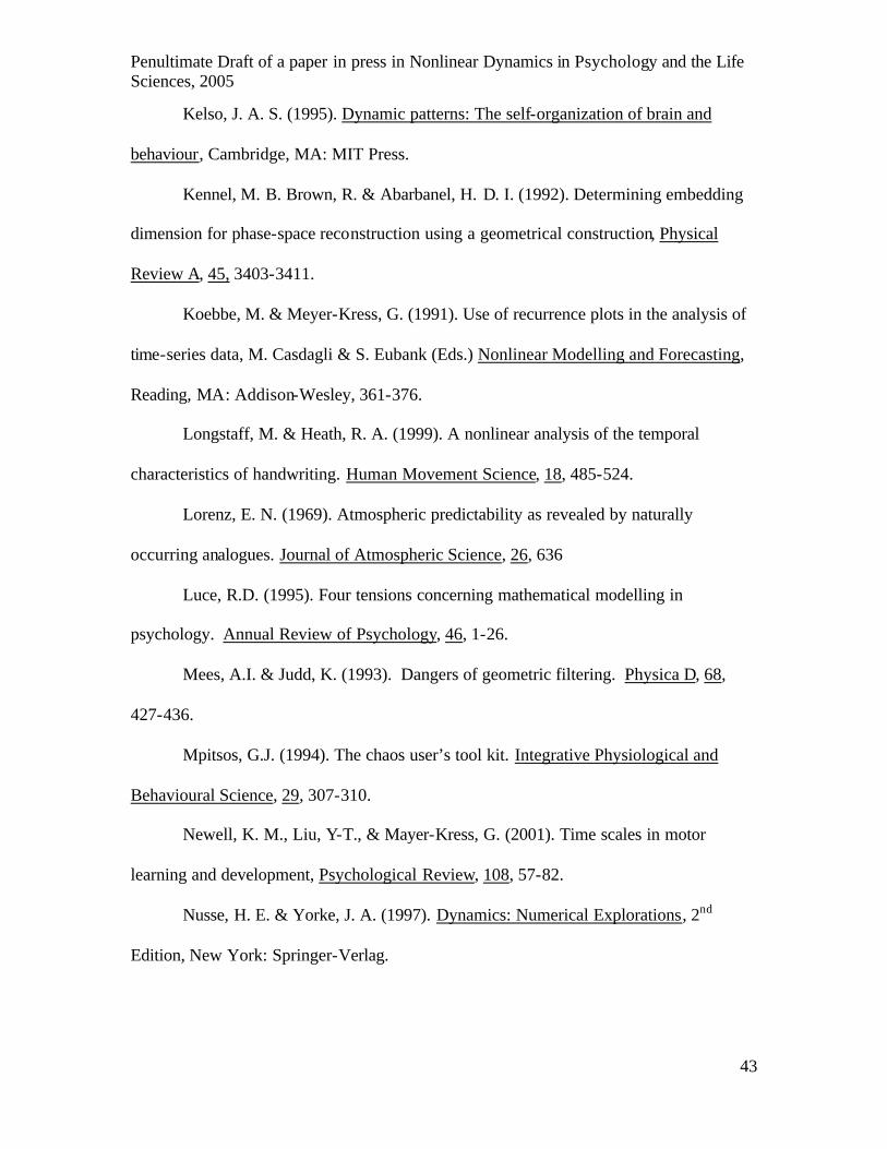
Penultimate Draft of a paper in press in Nonlinear Dynamics in Psychology and the Life Sciences, 2005
43
Kelso, J. A. S. (1995). Dynamic patterns: The self-organization of brain and
behaviour, Cambridge, MA: MIT Press.
Kennel, M. B. Brown, R. & Abarbanel, H. D. I. (1992). Determining embedding
dimension for phase-space reconstruction using a geometrical construction, Physical
Review A, 45, 3403-3411.
Koebbe, M. & Meyer-Kress, G. (1991). Use of recurrence plots in the analysis of
time-series data, M. Casdagli & S. Eubank (Eds.) Nonlinear Modelling and Forecasting,
Reading, MA: Addison-Wesley, 361-376.
Longstaff, M. & Heath, R. A. (1999). A nonlinear analysis of the temporal
characteristics of handwriting. Human Movement Science, 18, 485-524.
Lorenz, E. N. (1969). Atmospheric predictability as revealed by naturally
occurring analogues. Journal of Atmospheric Science, 26, 636
Luce, R.D. (1995). Four tensions concerning mathematical modelling in
psychology. Annual Review of Psychology, 46, 1-26.
Mees, A.I. & Judd, K. (1993). Dangers of geometric filtering. Physica D, 68,
427-436.
Mpitsos, G.J. (1994). The chaos user’s tool kit. Integrative Physiological and
Behavioural Science, 29, 307-310.
Newell, K. M., Liu, Y-T., & Mayer-Kress, G. (2001). Time scales in motor
learning and development, Psychological Review, 108, 57-82.
Nusse, H. E. & Yorke, J. A. (1997). Dynamics: Numerical Explorations, 2nd
Edition, New York: Springer-Verlag.

Penultimate Draft of a paper in press in Nonlinear Dynamics in Psychology and the Life Sciences, 2005
44
Osborne, A. R., & Provenzale, A. (1989). Finite correlation dimension for
stochastic systems with power- law spectra, Physica D, 35, 357-381.
Provenzale, A., Smith, L. A., Vio, R. & Murante, G. (1992). Distinguishing
between low-dimensional dynamics and randomness in measured time series, Physica D,
58, 31-49.
Rao, T. S., & Gabr, M. M. (1984). An introduction to bispectral analysis and
bilinear time series models, New York, Springer-Verlag.
Ratcliff, R. (1979). Group reaction time distributions and an analysis of
distribution statistics. Psychological Bulletin, 86, 446-461.
Roweis, S. T. & Lawrence, K. S. (2000) Nonlinear Dimensionality Reduction by
Locally Linear Embedding, Science, 290, 2323-2326.
Sauer, T., Yorke, J. & Casdagli, M. (1991). Embedology. Journal of Statistical
Physics, 65, 579-616.
Schmitz, A. & Schreiber, T. (1999). Testing for nonlinearity in unevenly sampled
time series, Physical Review E, 59, 4044-4047.
Schreiber, T. (1997). Detecting and analysing nonstationarity in a time series
using nonlinear cross predictions, Physical Review Letters, 78, 843-846.
Schreiber, T. (1998). Constrained randomisation of time series data, Physical
Review Letters, 80, 2105-2108.
Schreiber, T. (1999). Interdisciplinary application of nonlinear time series
methods, Physics Reports, 308, 1-64.
Schreiber, T. & Schmitz, A. (1997). Discrimination power of measures for
nonlinearity in a time series, Physical Review E, 55, 5443-5447.
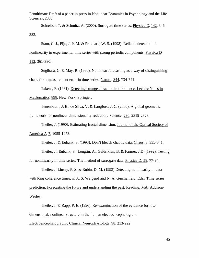
Penultimate Draft of a paper in press in Nonlinear Dynamics in Psychology and the Life Sciences, 2005
45
Schreiber, T. & Schmitz, A. (2000). Surrogate time series, Physica D, 142, 346-
382.
Stam, C. J., Pijn, J. P. M. & Pritchard, W. S. (1998). Reliable detection of
nonlinearity in experimental time series with strong periodic components. Physica D,
112, 361-380.
Sugihara, G. & May, R. (1990). Nonlinear forecasting as a way of distinguishing
chaos from measurement error in time series, Nature, 344, 734-741.
Takens, F. (1981). Detecting strange attractors in turbulence: Lecture Notes in
Mathematics, 898, New York: Springer.
Tenenbaum, J. B., de Silva, V. & Langford, J. C. (2000). A global geometric
framework for nonlinear dimensionality reduction, Science, 290, 2319-2323.
Theiler, J. (1990). Estimating fractal dimension. Journal of the Optical Society of
America A, 7, 1055-1073.
Theiler, J. & Eubank, S. (1993). Don’t bleach chaotic data. Chaos, 3, 335-341.
Theiler, J., Eubank, S., Longtin, A., Galdrikian, B. & Farmer, J.D. (1992). Testing
for nonlinearity in time series: The method of surroga te data. Physica D, 58, 77-94.
Theiler, J. Linsay, P. S. & Rubin, D. M. (1993) Detecting nonlinearity in data
with long coherence times, in A. S. Weigend and N. A. Gershenfeld, Eds., Time series
prediction: Forecasting the future and understanding the past. Reading, MA: Addison-
Wesley.
Theiler, J. & Rapp, P. E. (1996). Re-examination of the evidence for low-
dimensional, nonlinear structure in the human electroencephalogram.
Electroencephalographic Clinical Neurophysiology, 98, 213-222.

Penultimate Draft of a paper in press in Nonlinear Dynamics in Psychology and the Life Sciences, 2005
46
Thomasson, N., Hoeppner, T. J., Webber, C. L. & Zbilut, J. P. (2001). Recurrence
quantification in epileptic EEGs, Physics Letters A, 279, 94-101.
Tong, H. (1990). Non-linear time series, a dynamical system perspective. Oxford:
Oxford University Press.
Trulla, L. L., Giuliani, A., Zbilut, J. P. & Webber, C. L. (1996). Recurrence
quantification analysis of the logistic equation with transients, Physical Letters A, 223,
255-260.
Wand, M. P. & Jones, M. C. (1995). Kernel Smoothing. London: Chapman &
Hall.
Webber, C. L. & Zbilut, J. P. (1994). Dynamical assessment of physiological
systems and states using recurrence plot strategies. Journal of Applied Physiology, 76,
965-973.
Weigend, A. S. & Gershenfeld, N. A. (1993). Time series prediction: Forecasting
the future and understanding the past. Reading, MA: Addison-Wesley.

Penultimate Draft of a paper in press in Nonlinear Dynamics in Psychology and the Life Sciences, 2005
47
FIGURE CAPTIONS
Figure 1. a) 10000 x values (thin line) for the Lorenz differential equations:
( )xydtdx −= 10 , ( )yzxdtdy −−= 28 , and 38zxydtdz −= , solved with step
size=0.01 and starting from (x,y,z,t) = (0,1,0,0), with a Lowess (Cleveland, 1979) smooth
using a 1000 element moving window (thick line). The Lorenz series was generated using
the default settings of the Smalldyn program (http://keck2.umd.edu/dynamics, see Nusse
& Yorke, 1997). Analyses reported here examine the first 10000 values (data file
lorenz1.dat), values from t=2001-10 000 (lorenz2.dat) or values from t=2001-
100 000 (lorenz3.dat). (b) Filtered noisy Lorenz series from t=2001-10 000. Noise
was additive Gaussian with the same standard deviation as the Lorenz series (i.e. 50%
noise, n1.dat). The geometric filter was iterated six times, retaining two singular
values and using a minimum neighbourhood size of 400 in a 10 dimensions delay 1
embedding (ghkss n1.dat –i6 –q2 –k400 –m10 –d1 –o
n1q2k400.dat).
Figure 2. A plot of x(t) from Figure 1a against its derivative estimated at (a) lag one, and
(b) lag 12. Points in the derivative plot are joined to emphasise the trajectory of the
dynamics. In (a) t = 1…10000, whereas for (b) and (c) t = 2001…10000. In (a) points for
t=1…2000 are joined by a dotted line, and the four “spikes”, one pointing the left from
the top lobe and three pointing to the right from the bottom lobe, are caused by single
points with unusually large differences. Lag 12 difference plots for (c) the filtered 50%
noise series shown in Figure 1b, and (d) the 50% noise series filtered with the same
parameters as (c), but using a three rather than two-dimensional projection.

Penultimate Draft of a paper in press in Nonlinear Dynamics in Psychology and the Life Sciences, 2005
48
Figure 3. Space-time separation plots showing contours of constant probability for spatial
separation as a function of time separation from 1-500 for pairs of embedded point s from
(a) the series in Fig.1a from t =2001-10000 using a 5 dimensional delay 17 embedding
(stp lorenz2.dat -%0.1 -t500 -d17 –m5 -o) and (b) The Lorenz series
from t=2001-10000 with additive Gaussian noise of equal standard deviation and a 10
dimensional delay 1 embedding (stp n1.dat -d1 -m10 -%0.1 -t500 –o).
For parameter -%f, the algorithm calculates k contours, where k is the nearest integer less
than 1/f, at probability values 1/k,2/k…1. A weakness of this algorithm is that it produces
a noisy upper contour, as it is the sample maximum, which should not be given much
weight in examining the pattern in the space-time plot. The contour for the maximum
value has been omitted from (b) to provide clearer resolution of the lower contours.
Figure 4. Local slopes of log(C(ε)) vs. log(ε) plots for a range of distances, ε, and
embedding dimensions from 1 to 10 in a delay 17 embedding with a Theiler window of
100 (a) for the Lorenz series for t = 2001-100 000 (d2 lorenz3.dat –M1,10
-d17 –t100 -N0 –o), (b) the Lorenz series for t=2001-10000 (d2
lorenz2.dat –M1,10 -d17 –t100 -N0 –o), and the filtered noisy Lorenz
series (c) using 2 dimensional projection, as in Figures 1b and 2c (d2
n1q2k400i6.dat –M1,10 -d17 –t100 -N0 –o) and (d) 3 dimensional
projections, as in Figure 2d (d2 n1q3k400i6.dat –M1,10 -d17 –t100 -N0
–o). The -N0 option indicated that the computation should be done on all possible pairs
of points (the default is a maximum of 1000). Lower lines indicate lower embedding
dimensions. The dashed line in each panel indicates the true dimension, 2.05.

Penultimate Draft of a paper in press in Nonlinear Dynamics in Psychology and the Life Sciences, 2005
49
Figure 5. One-step cross prediction errors obtained using 10 sequential 1000 element
segments (separate lines) to obtain predictions for all segments (abscissa) for (a) the
series in Fig.1a using a 5 dimensional delay 17 embedding and a minimum
neighbourhood size of 30 (nstat_z lorenz1.dat -#10 –m5 –d17 –k30 -o)
and (b) the series in Fig.1a plus Gaussian noise with double the standard deviation of the
Lorenz series using a 10 dimensional, delay 1 embedding and a minimum neighbourhood
size of 30 (nstat_z lorenz1.dat -#10 –m10 –d1 –k40 -o).
Figure 6. Histograms of standardised root mean squared one-step prediction error (Z) in a
10 dimensional delay one embedding for original (filled bar) and surrogate (unfilled bars)
series (a) 50% Noise and 1.6 standard deviation (SD) neighbourhood radius (predict
n1.dat n4.dat_surr_0?? –m10 –d1 –v1.6 -o), (b) 66.6% Noise and a 1.6
SD neighbourhood radius (predict n2.dat n4.dat_surr_0?? –m10 –d1 –
v1.6 -o), and (c) 80% Noise and a 2.6 SD neighbourhood radius (predict n4.dat
n4.dat_surr_0?? –m10 –d1 –v2.6 -o). (d) 14 step prediction error for the
80% noise series with a 1.6 SD neighbourhood radius (predict n4.dat
n4.dat_surr_0?? –m10 –d1 –v1.6 –o –s14). The predict program
outputs root mean squared prediction error; standardization used the mean and standard
deviation of the surrogate data.
Figure 7. Root mean square locally constant prediction error as a function of prediction
lag for (a) 50% and 66.6% noise series with a 1.6 standard deviation (SD) neighbourhood
radius, (b) 80% noise series with a 1.6 SD radius and a 2.6 SD radius, and (c) coarsely
sampled 80% noise series, with a 1.6 SD radius. The symbols are prediction error for the

Penultimate Draft of a paper in press in Nonlinear Dynamics in Psychology and the Life Sciences, 2005
50
original series. The solid line is the mean prediction error for the 99 surrogate series. The
dotted lines are a 95% confidence interval for surrogate prediction, estimated by the 3rd
and 97th order statistics of the surrogate distribution.
Figure 8. (a) Squared correlation between the original Lorenz series from t=2001-10000
and filtered series, and (b) the standard deviation (SD) of the filtered series, as a function
of filter iterations retaining one to three singular values (q1-q3). For the 50% noise series,
minimum neighbourhood size was either 5% (k400) or 10% (k800) of the series length,
whereas for the 80% noise series it was 10% (k800) or 20% (k1600) of the series length.
The standard deviation of the original Lorenz series (6.2) is indicated by a solid flat line
in (b) and (c).
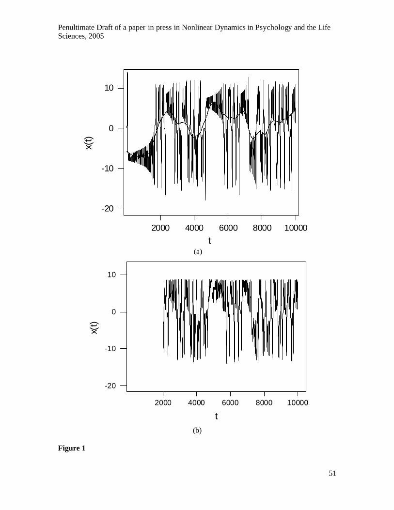
Penultimate Draft of a paper in press in Nonlinear Dynamics in Psychology and the Life Sciences, 2005
51
2000 4000 6000 8000 10000
-20
-10
0
10
t
x(t)
(a)
2000 4000 6000 8000 10000
-20
-10
0
10
t
x(t)
(b)
Figure 1

Penultimate Draft of a paper in press in Nonlinear Dynamics in Psychology and the Life Sciences, 2005
52
76543210-1-2-3
10
0
-10
-20
x(t)-x(t-1)
x(t)
(a)
100-10-20
10
0
-10
-20
x(t)-x(t-12)
x(t)
(b)
Penultimate Draft of a paper in press in Nonlinear Dynamics in Psychology and the Life Sciences, 2005
53
100-10
10
5
0
-5
-10
-15
x(t)-x(t-12)
x(t)
(c)
-20 -10 0 10
-20
-10
0
10
x(t)-x(t-12)
x(t)
(d)
Figure 2
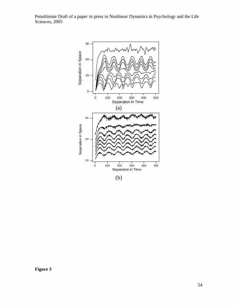
Penultimate Draft of a paper in press in Nonlinear Dynamics in Psychology and the Life Sciences, 2005
54
5004003002001000
30
20
10
0
Separation in Time
Sep
arat
ion
in S
pace
(a)
0 100 200 300 400 500
10
20
30
Separation in Time
Sep
erat
ion
in S
pace
(b)
Figure 3
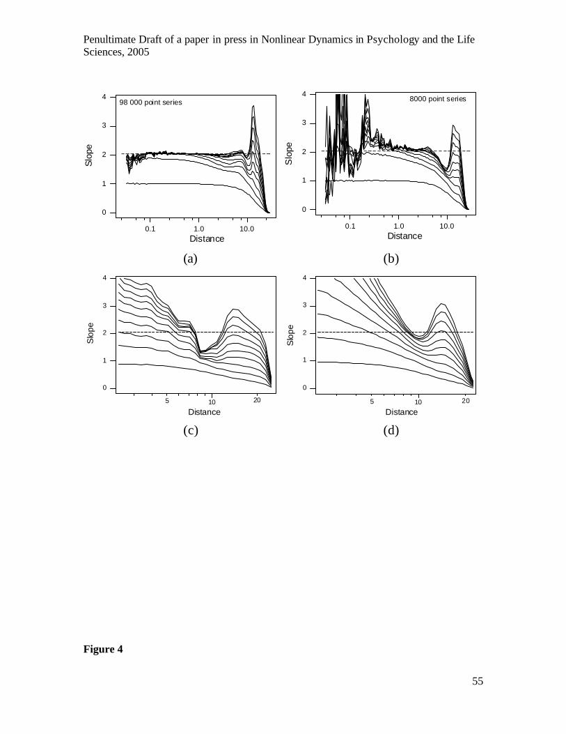
Penultimate Draft of a paper in press in Nonlinear Dynamics in Psychology and the Life Sciences, 2005
55
10.01.00.1
4
3
2
1
0
Distance
Slo
pe98 000 point series
10.01.00.1
4
3
2
1
0
Distance
Slo
pe
8000 point series
(a) (b)
10
4
3
2
1
0
Distance
Slo
pe
205 10
0
1
2
3
4
Distance
Slo
pe
205
(c) (d)
Figure 4

Penultimate Draft of a paper in press in Nonlinear Dynamics in Psychology and the Life Sciences, 2005
56
10987654321
2
1
0
Segment being Predicted
Rel
ativ
e P
redi
ctio
n E
rror segment 1
Predictions by
segment 2Predictions by
(a)
1 2 3 4 5 6 7 8 9 10
0.9
1.0
1.1
1.2
Segment being Predicted
Rel
ativ
e P
redi
cito
n E
rror
Predictions bysegment 1
Predictions bysegment 2
(b)
Figure 5

Penultimate Draft of a paper in press in Nonlinear Dynamics in Psychology and the Life Sciences, 2005
57
-8 -4 0
0
5
10
15
Z
Freq
uenc
y
Z = -7.13
3210-1-2-3-4
10
5
0
Z
Fre
quen
cy
Z = -3.18
(a) (b)
3210-1-2-3
15
10
5
0
Z
Freq
uenc
y
Z = -2.18
-6 -5 -4 -3 -2 -1 0 1 2 3 4
0
5
10
15
Z
Fre
quen
cy
Z = -5.26
(c) (d)
Figure 6

Penultimate Draft of a paper in press in Nonlinear Dynamics in Psychology and the Life Sciences, 2005
58
50403020100
11
10
9
8
7
Prediction Lag
Pre
dict
ion
Err
or
50% Noise
66.6% Noise
(a)
403020100
14.0
13.8
13.6
13.4
13.2
13.0
Prediction Lag
Pre
dict
ion
Err
or
2.6 SD Neighbourhood 1.6 SD Neighbourhood
80% Noise
(b)
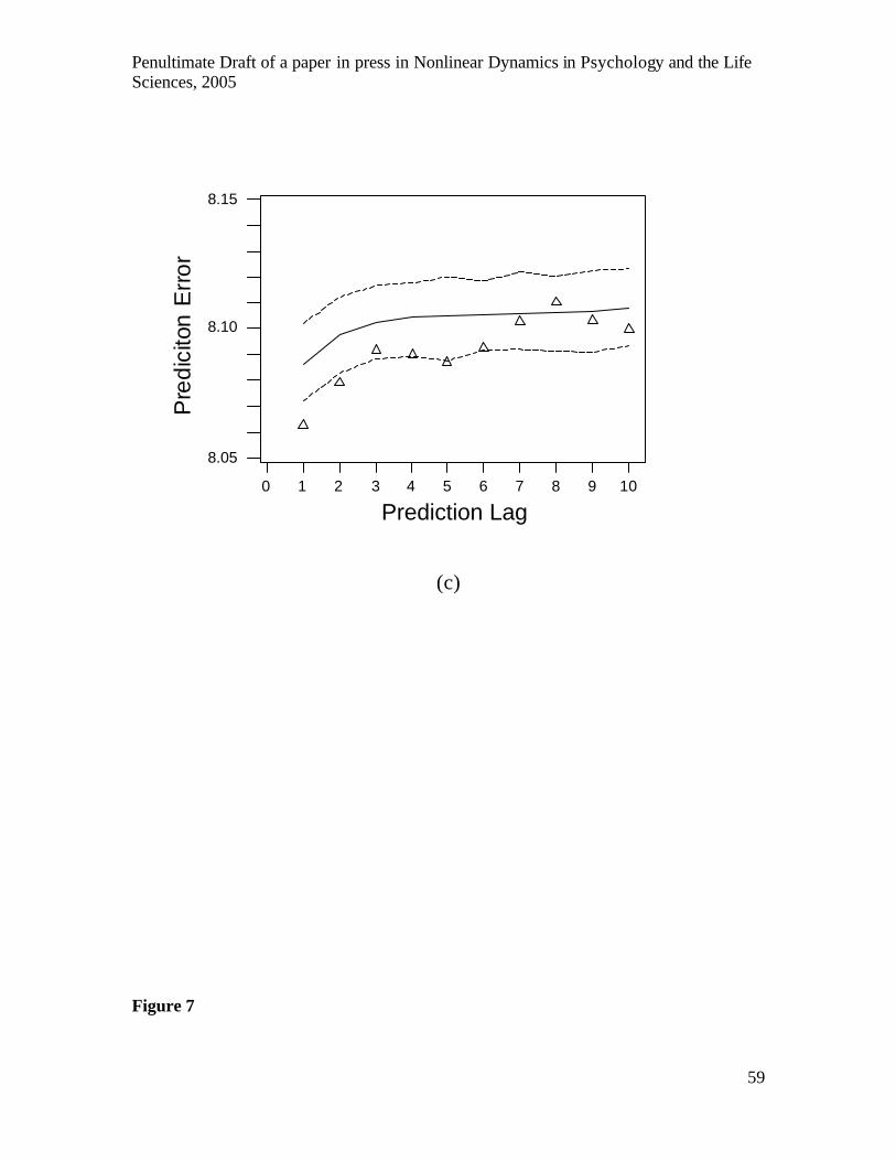
Penultimate Draft of a paper in press in Nonlinear Dynamics in Psychology and the Life Sciences, 2005
59
0 1 2 3 4 5 6 7 8 9 10
8.05
8.10
8.15
Prediction Lag
Pre
dici
ton
Err
or
(c)
Figure 7
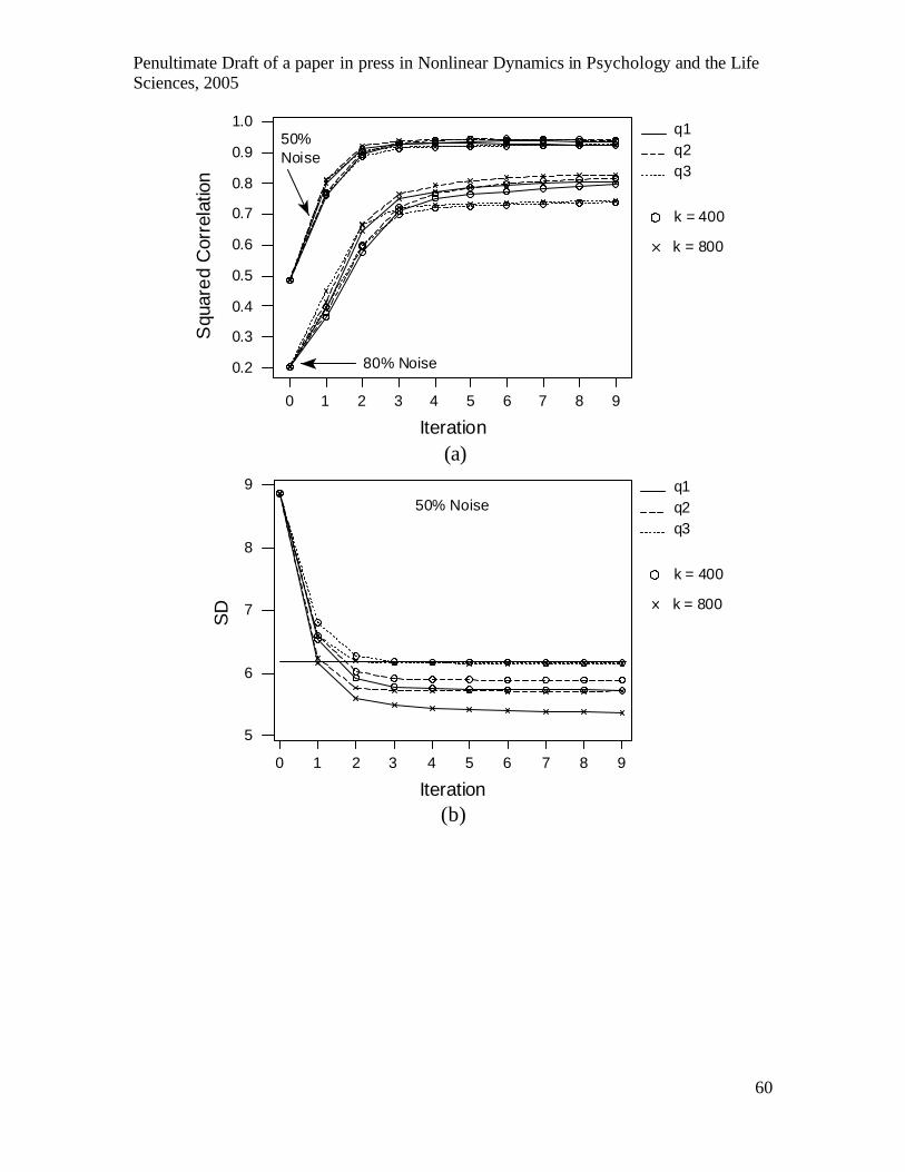
Penultimate Draft of a paper in press in Nonlinear Dynamics in Psychology and the Life Sciences, 2005
60
9876543210
1.0
0.9
0.8
0.7
0.6
0.5
0.4
0.3
0.2
Iteration
Squ
ared
Cor
rela
tion
k = 800
k = 400
q3 q2 q1
50%Noise
80% Noise
(a)
0 1 2 3 4 5 6 7 8 9
5
6
7
8
9
Iteration
SD k = 800
k = 400
q3 q2 q1
50% Noise
(b)
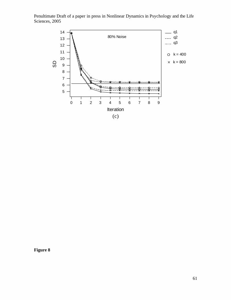
Penultimate Draft of a paper in press in Nonlinear Dynamics in Psychology and the Life Sciences, 2005
61
q1 q2 q3
k = 400
k = 800
0 1 2 3 4 5 6 7 8 9
5
6
7
8
9
10
11
12
13
14
Iteration
SD
80% Noise
(c)
Figure 8